PASJ: Publ. Astron. Soc. Japan , 1–??,c⃝ 2015. Astronomical Society of Japan.

— Review —Rotation Curve and Mass Distribution in the Milky Way and Spiral

Galaxies

Yoshiaki SofueInstitute of Astronomy, The University of Tokyo, Mitaka, 181-0015 Tokyo

Email:sofue@ioa.s.u-tokyo.ac.jp

(Received 2015 0; accepted 2015 0)

Abstract

Rotation curves are the major tool for determining the distribution of mass in spiral galaxies, whichis the most fundamental quantity for the dynamics of galaxies. In this paper we review the progressin the studies of rotation curves and mass distribution in spiral galaxies. In chapters II and III wedescribe the methods to derive rotation curves in the Milky Way and spiral galaxies, respectively. Thebasic characteristics of observed rotation curves are discussed in relation to the galaxy properties. Inchapter IV we describe dynamical methods to determine the mass distribution in the Milky Way andspiral galaxies based on the Virial theorem, which are categorized into decomposition and direct methods.In the decomposition method, a rotation curve is fitted by the least χ2 method to a model curve assumingseveral mass components such as a central massive object, bulge, disk and dark halo. In the direct method,the mass distribution is directly calculated using rotation velocities without employing mass models. Wealso describe statistical relations among determined dynamical parameters of galaxies.

Key words: Galaxy: dynamics – galaxies: rotation curve – galaxies: kinematics and dynamics –galaxies: dark matter – galaxies: structure

1. INTRODUCTION

The mass of a galaxy and its distribution are obtainedby two ways: one is the photometric method to derive theluminous mass, where we use luminosity profiles by assum-ing the mass-to-luminosity (M/L) ratio, and the other isthe dynamical method, where the Virial three is appliedto kinematical data such as rotation curves to calculatethe dynamical mass.

The luminous mass is occupied by stars and interstellarmatter. Hence, the stellar luminosity distribution roughlyrepresents the luminous mass distribution. In the decadesit has been firmly known that the luminous mass cannotexplain the entire dynamical mass. The discrepancy be-tween the luminous and dynamical masses increases withthe radius. The invisible dynamical mass is called thedark matter, which dominates in the outermost regions ofgalaxies composing the dark halo.

Although the photometric method is convenient to ap-proximately map the luminous mass, it varies with theemployed M/L ratio, for which independent measurementof mass is in any way necessary beforehand. Besides theambiguity of the assumed M/L ratio, it cannot give infor-mation about invisible mass such as a black hole and darkmatter, which are one of the most interested subjects ofgalaxy dynamics.

For determination of the distribution of dark matterand invisible mass like black holes, the dynamical methodis the essential tool. In the method, it is assumed thata galaxy is dynamically relaxed and the Virial theorem

R (kpc)1 10 1000.10.01

300

200

100

0

V

(km/s)

BH

Bulge

Disk

Dark Halo

Satellite

galaxiesGlobular

clusters

Rotation Curve

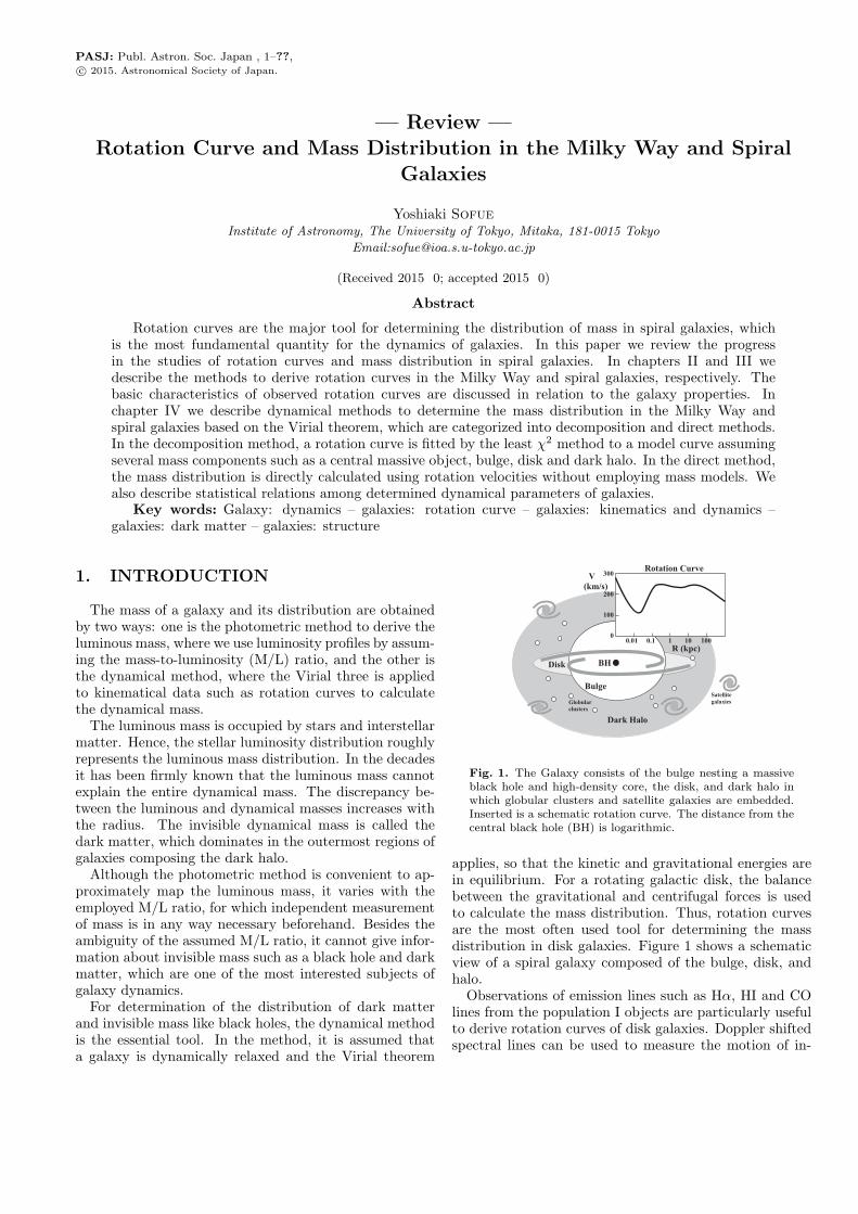
Fig. 1. The Galaxy consists of the bulge nesting a massiveblack hole and high-density core, the disk, and dark halo inwhich globular clusters and satellite galaxies are embedded.Inserted is a schematic rotation curve. The distance from thecentral black hole (BH) is logarithmic.

applies, so that the kinetic and gravitational energies arein equilibrium. For a rotating galactic disk, the balancebetween the gravitational and centrifugal forces is usedto calculate the mass distribution. Thus, rotation curvesare the most often used tool for determining the massdistribution in disk galaxies. Figure 1 shows a schematicview of a spiral galaxy composed of the bulge, disk, andhalo.

Observations of emission lines such as Hα, HI and COlines from the population I objects are particularly usefulto derive rotation curves of disk galaxies. Doppler shiftedspectral lines can be used to measure the motion of in-

2 Y. Sofue [Vol. ,

terstellar gas and population I objects. In these lines,velocity dispersion is negligibly small compared to rota-tion velocity, which allows us to neglect the pressure termand apply the simple balance of the gravity with the cen-trifugal force.

In Chapters II and III we review the methods to de-termine rotation curves of the Galaxy and spiral galaxies,respectively, and describe the general characteristics of ro-tation curves. The progress in the rotation curve studieswill be also reviewed briefly. Figures 2 and 3 whose theprogress in the decades of the rotation curves of the MilkyWay and the Andromeda galaxy.

In Chapter IV we review the methods to determine themass distributions in disk galaxies, and describe the dy-namical mass structure in spiral galaxies.

There have been a number of articles and reviews onrotation curves and dynamics of galaxies that includeBinney and Tremain (1987), Sofue and Rubin (2001),Sofue (2013a), and the literature therein. Elliptical galax-ies are out of the scope of this review. Considerationsthat employ unconventional physical laws such as MOND(modified Newtonian dynamics) to explain the observedrotation curves are also out of the scope of this review.

2. ROTATION CURVE OF THEMILKY WAY

1. Galactic constants

1.1. Solar position and Mass inside the solar circle

The dynamical mass of the Galaxy on the order of∼ 1011M⊙ inside the solar circle was already calculatedearly in 1950’s (Oort 1958), when the circular orbit of thelocal standard of rest (LSR) was obtained in terms of thegalactic-centric distance R0and rotation velocity V0(Fichand Tremaine 1991 for a review).

In this paper, we use the galactic constants of(R0, V0)=(8.0 kpc, 200 km s−1), or, otherwise men-tioned, (R0,V0)=(8.0 kpc, 238 km s−1) from VERA (VLBIExperiment for Radio Astrometry) observations of propermotions and radial velocities of maser sources (Honma etal. 2012; 2015). For a set of the parameters of R0= 8 kpcand V0= 200 to 238 km s−1, the most fundamental quan-tity, the mass inside the solar circle on an assumption ofspherical distribution, is given by

M0 =R0V

20

G= (7.44 to 1.05)× 1010M⊙ ∼ 1011M⊙, (1)

where G is the gravitational constant. Although this ap-proximate estimation is not far from the true value, themass distribution in the Galaxy is not simply spherical,and it is principally derived by analyzing the rotationcurves on the assumption that the centrifugal force of thecircular motion is balancing with the gravitational forcein a spheroid or a disk. Hence, the first step to derive themass distribution is to obtain the rotation curve.

R (kpc)

V(km/s)

Honma et al. 2015

0 2 4 6 8 10 12 14 16 18 200

100

200

300

V(km/s)

R (kpc)10

-410

-310

-210

-110

010

110

20

100

200

300

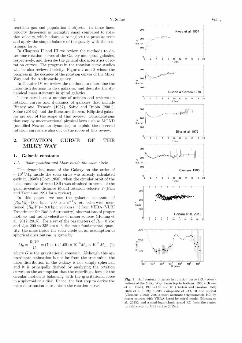
Fig. 2. Half century progress in rotation curve (RC) obser-vations of the Milky Way. From top to bottom: 1950’s (Kweeet al. 1954); 1970’s CO and HI (Burton and Gordon 1978;Blitz et al 1979); 1980’s Composite of CO, HI and optical(Clemens 1985); 2001’s most accurate trigonometric RC bymaser sources with VERA fitted by spiral model (Honma etal. 2015); and a semi-logarithmic grand RC from the centerto half a way to M31 (Sofue 2015a).

No. ] Review: Rotation and Mass of Galaxies 3

R (kpc)

V(km/s)

0.1 1 10 1000

100

200

300

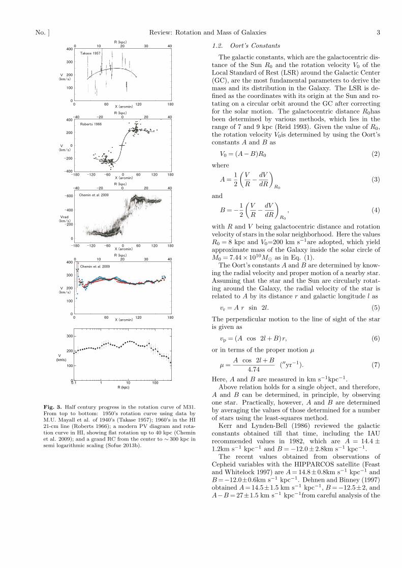
Fig. 3. Half century progress in the rotation curve of M31.From top to bottom: 1950’s rotation curve using data byM.U. Mayall et al. of 1940’s (Takase 1957); 1960’s in the HI21-cm line (Roberts 1966); a modern PV diagram and rota-tion curve in HI, showing flat rotation up to 40 kpc (Cheminet al. 2009); and a grand RC from the center to ∼ 300 kpc insemi logarithmic scaling (Sofue 2013b).

1.2. Oort’s Constants

The galactic constants, which are the galactocentric dis-tance of the Sun R0 and the rotation velocity V0 of theLocal Standard of Rest (LSR) around the Galactic Center(GC), are the most fundamental parameters to derive themass and its distribution in the Galaxy. The LSR is de-fined as the coordinates with its origin at the Sun and ro-tating on a circular orbit around the GC after correctingfor the solar motion. The galactocentric distance R0hasbeen determined by various methods, which lies in therange of 7 and 9 kpc (Reid 1993). Given the value of R0,the rotation velocity V0is determined by using the Oort’sconstants A and B as

V0 = (A−B)R0 (2)

where

A =12

(V

R− dV

dR

)R0

(3)

and

B = −12

(V

R− dV

dR

)R0

, (4)

with R and V being galactocentric distance and rotationvelocity of stars in the solar neighborhood. Here the valuesR0 = 8 kpc and V0=200 km s−1are adopted, which yieldapproximate mass of the Galaxy inside the solar circle ofM0 = 7.44× 1010M⊙ as in Eq. (1).

The Oort’s constants A and B are determined by know-ing the radial velocity and proper motion of a nearby star.Assuming that the star and the Sun are circularly rotat-ing around the Galaxy, the radial velocity of the star isrelated to A by its distance r and galactic longitude l as

vr = A r sin 2l. (5)

The perpendicular motion to the line of sight of the staris given as

vp = (A cos 2l +B)r, (6)

or in terms of the proper motion µ

µ =A cos 2l +B

4.74(′′yr−1). (7)

Here, A and B are measured in km s−1kpc−1.Above relation holds for a single object, and therefore,

A and B can be determined, in principle, by observingone star. Practically, however, A and B are determinedby averaging the values of those determined for a numberof stars using the least-squares method.

Kerr and Lynden-Bell (1986) reviewed the galacticconstants obtained till that time, including the IAUrecommended values in 1982, which are A = 14.4 ±1.2km s−1 kpc−1 and B = −12.0± 2.8km s−1 kpc−1.

The recent values obtained from observations ofCepheid variables with the HIPPARCOS satellite (Feastand Whitelock 1997) are A = 14.8±0.8km s−1 kpc−1 andB =−12.0±0.6km s−1 kpc−1. Dehnen and Binney (1997)obtained A=14.5±1.5 km s−1 kpc−1, B =−12.5±2, andA−B =27±1.5 km s−1 kpc−1from careful analysis of the

4 Y. Sofue [Vol. ,

compiled circular velocities and consideration of the val-ues from the literature. Similar values were also obtainedfrom red giants using infrared photometric data (Mignard2000).

1.3. Dynamical parameters representing the Galaxy

In this review, the galactic mass distribution is obtainedby Virial thorem based on the analysis of rotation curves.As the definition of rotation curve, we first assume thatthe motion of gas and stars in the Galaxy is circular. Thisassumption put a significant limitation on the obtainedresults. In fact, the galactic motion is superposed by non-circular streams such as due to a bar, spiral arms, and ex-panding rings. The dynamical parameters of the Galaxyto be determined from observations are those representingaxisymmetric and non-axisymmetric structures. In table1, we list the representative parameters and analysis meth-ods (Sofue 2013b). In the present paper, we review themethods to obtain parameters (1) to (10) in the table,which define the axisymmetric structure of the Galaxy asthe first approximation to the fundamental galactic struc-ture.

Non-circular motions have often been discussed in rela-tion to the central dynamics caused by a bar, which arerecognized as ’forbidden’ velocities in longitude-radial ve-locity diagrams (LV diagrams) (e.g., Binney et al. 1991;Jenkins and Binney 1994; Athnasoula 1992; Burton andLiszt 1993). These motions are the manifestation of non-axisymmetric mass distributions in the galactic disk, andmay be represented by the second-order parameters (11)to (27). However, these structures are beyond the scopeof this review, in which we concentrate ourselves on therotation curves and derived mass distributions.

2. Progress in Galactic rotation curve determi-nation

Figure 2 shows the progress in the determination of ro-tation curve of the Milky Way Galaxy. The rotation ofthe Milky Way is clearly seen in longitude-radial velocity(LV) diagrams along the galactic plane, where spectralline intensities are plotted on the (l,Vlsr) plane. Figure 5shows observed LV diagrams in the λ21-cm HI and λ2.6-mm CO emission lines for the entire disk of the Galaxy,and figure 8 shows those in the CO line for the GalacticCenter region.

The inner rotation curve of the Milky Way is simplymeasured by the terminal (tangential)-velocity methodapplied to radio line observations such as the HI andCO lines. The central mass condensation and the nuclearmassive black hole have been measured since 1980’s whenkinematics of interstellar gas and stars close to Sgr A∗, ourGalaxy’s nucleus, were measured by infrared observations.

The positive- and negative-velocity envelopes (terminalvelocities) at 0 < l < 90 and 270 < l < 360, respectively,are used for determining the inner rotation curve insidethe solar circle at R ≤ R0. This terminal (tangential)-velocity method is applied to HI and CO line observationsfor the inner Galaxy (Burton and Gordon 1978; Clemens

1985; Fich et al. 1989).In order to derive outer rotation curve beyond the solar

circle, optical distances and velocities of OB stars are com-bined with CO-line velocities (Blitz et al. 1982; Demersand Battinelli 2007). The HI thickness method is also use-ful to obtain rotation curve of the entire disk (Merrifield1992; Honma and Sofue 1997). High accuracy measure-ments of parallax and proper motions of maser sourcesand Mira variable stars using VLBI technique are provid-ing an advanced tool to derive a more accurate rotationcurve (Honma et al. 2007). It is only recent that propermotions of a considerable number of stars are used for ro-tation curve measurement (Lopez-Corredoira et al. 2014).

The most powerful tool to date to derive an accuraterotation curve of the Milky Way up to R ∼ 20 kpc is theVERA, with which trigonometric determination of boththe 3D positions and velocities is available simultaneouslyfor individual maser sources (Honma et al. 2007; 2012;2015; Sakai et al 2015; Nakanishi et al. 2015).

For the total mass of the Galaxy including the darkhalo, outer rotation curve and detailed analyses of motionsof satellite galaxies in the Local Group are used. The totalmass of the Galaxy including the dark halo up to ∼ 150kpc is estimated to be ∼ 3× 1011M⊙ by considering theouter rotation curve and motions of satellite galaxies.

3. Methods to determine galactic rotation curve

3.1. Terminal-velocity method inside the Solar circle

The galactic disk within the solar circle has tangentialpoints at which the rotation velocity is parallel to theline of sight (4). Figure 6 shows the tangent velocitiesmeasured for the 1st quadrant of the galactic disk (e.g.,Burton and Gordon 1978).

The maximum radial velocity vr max is called the termi-nal velocity or the tangent-point velocity. The tangent ve-locities are measured using spectral profiles of interstellargases as observed in the HI 21-cm and CO 2.6-mm emis-sion lines in the first and third quadrants of the galacticplane (0<l < 90 and 270<l < 360). Using this terminalvelocity, the rotation velocity V (R) is simply calculatedby

V (R) = vr max +V0 sin l, (8)

and the galacto-centric distance is given by

R = R0 sin l. (9)

3.2. Radial velocity method

Given the galactic constants R0 and V0, the rotationvelocity V (R) in the galactic disk can be obtained as afunction of galacto-centric distance R by measuring thedistance r and radial velocity vr (Fig. 4). The velocityvector of a star at any position in the Galaxy is determinedby observing its three dimensional position (r, l, b) andits motion (vr, vp), where vr is the radial velocity and vp

the perpendicular velocity with vp = µr with µ being theproper motion on the ski.

No. ] Review: Rotation and Mass of Galaxies 5

Table 1. Dynamical parameters for the Galactic mass determination†.

Subject Component No. of ParametersI. Axisymmetric structure Black hole (1) Mass— RC analysis— Bulge(s)‡ (2) Mass

(3) Radius(4) Profile (function)

Disk (5) Mass(6) Radius(7) Profile (function)

Dark halo (8) Mass(9) Scale radius(10) Profile (function)

II. Non-axisymm. structure Bar(s) (11) Mass(out of RC analysis) (12) Major axial length

(13) Minor axial length(14) z-directional axial length(15) Major axis profile(16) Minor axis profile(17) z-directional profile(18) Position angle(19) Pattern speed Ωp

Arms (20) Density amplitude(21) Velocity amplitude(22) Pitch angle(23) Position angle(24) Pattern speed Ωp

III. Radial flow Expanding rings (25) Mass(out of RC analysis) (26) Velocity

(27) Radius

† In the present paper we review on subject I.‡ The bulge and bar may be multiple, increasing the number of parameters.

Table 2. Rotation curves of the Milky Way Galaxy

Authors (year) Raddii Method Remark

Burton and Gordon (1978) 0 - 8 kpc HI tangent RCBlitz et al. (1979) 8 - 18 kpc OB-CO association RCClemens (1985) 0 -18 kpc CO/compil. RCDehnen and Binney (1998) 8 - 20 compil. + model RC/Gal. Const.Battinelli, et al. (2013) 9 - 24 kpc C stars RCBhattacharjee et al.(2014) 0 - 200 kpc Non-disk objects RC/model fitLopez-Corredoira (2014) 5 - 16 kpc Red-clump giants µ RCBobylev (2013); — & Bajkova (2015) 5 - 12 kpc Masers/OB stars RC/Gal. const.Honma et al. (2012, 2013, 2015) 3 - 20 kpc Masers, VLBI RC/Gal. const.Sofue et al. (2009); Sofue (2013b, 2015a) 0 - 300 kpc CO/HI/opt/compil. RC/model fit

1.

http://www.ioa.s.u-tokyo.ac.jp/∼sofue/h-rot.htm

6 Y. Sofue [Vol. ,

Fig. 4. [Top] Rotation velocity at any point in the galacticplane is obtained by measuring the distance r and the radialvelocity vr or the perpendicular velocity vp = µr, where µis proper motion. [Bottom] Rotation curve inside the solarcircle (R < R0; dashed circle) is obtained by measuring theterminal radial velocity vmax at the tangent point, where theGC distance is given by R = R0 sin l.

The galacto-centric distance R is calculated from theposition of the object (l, b,r) and R0 as

R = (r2 +R20 − 2rR0 cos l)1/2. (10)

Here, the distance r to the object must be measured di-rectly by trigonometric (parallax) method, or indirectlyby spectroscopic measurements.

If the orbit of the star is assumed to be circular in thegalactic plane, the rotation velocity V (R) may be obtainedby measuring one of the radial velocity or proper motion.The rotation velocity V (R) is related to the radial velocityvr as

V (R) =R

R0

( vr

sin l+V0

). (11)

The method using radial velocity has been traditionallyapplied to various stellar objects. Star forming regions aremost frequently used to determine the rotation curve be-yond the solar circle. In this method, distances r of OBstars are measured from their distance modulus from theapparent magnitude after correction for extinction andabsolute luminosity by the star’s color and spectral type.Then, the star’s distance r is assumed to be the same asthat of its associated molecular cloud and/or HII region

Fig. 5. Longitude-radial velocity (l − Vlsr) diagram of theλ21-cm HI line emission (top: Nakanishi 2007) and λ2.6-mmCO (bottom: Dame et al. 1985) lines along the galactic plane.(Figures courtesy by H. Nakanishi)

Fig. 6. CO and HI line tangent velocities for the inner rota-tion curve (Burton and Gordon 1978)

whose radial velocity is obtained by observing the Dopplervelocity of molecular lines and/or recombination lines. Inthis method, the error in the distance is large, which re-sults in the large scatter in the obtained outer rotationcurve, as seen in Fig. 2.

3.3. Proper motion method

Alternatively, the rotation velocity can be also deter-mined by measuring the proper motion µ as

V (R) = −R

s(vp +V0 cos l), (12)

where

s = r−R0 cos l, (13)

where vp = µr.VLBI observations have made it possible to employ

trigonometric (parallax) measurements of maser-line radio

No. ] Review: Rotation and Mass of Galaxies 7

Fig. 7. Circular velocities obtained from proper motionsof red-clump giant stars and an averaged rotation curve(Lopez-Corredoira 2014). The LSR circular velocity is as-sumed to be V0 = 238 km s−1.

sources to determine the distance r and the proper motionvp (= rµ), as well as the radial velocity vr at the same timefrom radio spectroscopy of the maser line. Applying thistechnique to a number of maser sources, the outer rotationcurve has been determined in a higher accuracy (Honmaet al. 2012, 2015; Sakai et al. 2012, 2015; Nakanishi et al.2015) (figure 2.

A large number of stellar proper motions fromHYPPARCOS observations combined with the 2MASSphotometric data have recently been analyzed for galac-tic kinematics. Figure 7 shows the most recent rotationcurve derived by the proper motion method applied to redclump giant stars (Roeser et al 2010; Lopez-Corredoira2014). Proper motions were obtained from PPMXS cata-logue from HIPPARCOS observations, and the distanceswere determined from K and J band photometry using2MASS star catalogue correcting for the interstellar ex-tinction. The RCG stars were used for their assumedconstant absolute magnitudes.

3.4. Ring thickness method

The HI-disk thickness method utilizes apparent width ofan annulus ring of HI disk in the whole Galaxy (Merrifield1992; Honma and Sofue 1997). This method yieldsannulus-averaged rotation velocity in the entire galacticdisk. The apparent latitudinal angle ∆b of the HI diskalong an annulus ring of radius R varies with longitude as

∆b = arctan

(z0

R0 cos l +√

R2 −R20 sin 2l

). (14)

with

vr = W (R) sin l, (15)

where

W (R) =[V (R)

R0

R−V0

]. (16)

The amplitude of ∆b normalized by its value at l = 180plotted against longitude l is uniquely related to thegalacto-centric distance R, which is as a function of V (R)and is related to vr as above equations. This method uti-lizes the entire HI disk, so that they obtained rotationcurve manifests an averaged kinematics of the Galaxy.Therefore, it is informative for more global rotation curve

compared to the measurements of individual stars or thetangent-point method.

3.5. VLBI trigonometric method

The ultimate method to derive accurate rotation curveof the Milky Way, without being bothered by variousassumptions such as the circular rotation and/or a pri-ori given solar constants, would be the VLBI method bywhich we can determine the 3D positions and motions ofindividual maser sources. The VERA observations havemost successfully obtained rotation velocities for abouthundred galactic maser sources within ∼ 10 kpc from theSun, as well as the solar constants (Honma et al. 2007;2012; 2015; Sakai et al 2015; Nakanishi et al. 2015).

4. Central Rotation Curve

The Galaxy provides a unique opportunity to derivea high resolution central rotation curve. Proper-motionstudies in the near infrared have revealed individual or-bits of stars within the central 0.1 pc, and the velocitydispersion increases toward the center, indicating the ex-istence of a massive black hole of mass 3×106M⊙ (Genzelet al. 1994, 1997, 2000, 2010; Ghez et al. 1998, 2005, 2008;Rieke and Rieke 1988; Lindqvist et al. 1992; Gillessen etal. 200x).

The mass structure between the central black hole andthe disk, and therefore, the dynamical mass structure in-side the bulge, is not thoroughly studied. In figure 8we show a longitude-velocity (LV) diagram of the cen-tral molecular disk as obtained from the Coloumbia COline survey (Dame et al. 2001), Nobeyama 45-m GalacticCenter survey (Oka et al. 1998), and an CO line LV di-agram observed with the NRO 45-m telescope at a 15′′with 7′′.5 Niquist-sampling gridding. The figures showthat most of the molecular gas is distributed on the tiltedridges, representing the rotating central molecular disk.The tilted ridges make the fundamental structure in theLV diagram.

By applying the terminal velocity method to each LVridge in figure 8, we determine rotational velocities on in-dividual LV ridges. The obtained terminal velocities areshown in figure 9. The velocities are scattered locally by20-30 km s−1. The east-west asymmetry in velocity dis-tribution is greater than the local scatter, and amountsto almost 30-40 km s−1. Open circles in figure 9 showsa rotation curve produced from the thus measured termi-nal velocities. The filled circles in the bottom panel infigure 9 show running-averaged values every 1.3 times theneighboring radius with a Gaussian weighting width of 0.3times the radius.

5. Rotation Curve of the Bulge, Disk and DarkHalo

The entire rotation curve of the Galaxy is obtained bycombining the observed rotation velocities from the vari-ous methods. A unified rotation curve was obtained by in-tegrating the existing data by re-calculating the distances

8 Y. Sofue [Vol. ,

(a)

VE

LO

-LS

R

Galactic Long.

300

200

100

0

-100

-200

-30010 0 350

(b)

0 10 20 30 40

VE

L-L

SR

GALACTIC LONG.01 00 00 30 00 -00 30 -01 00

200

150

100

50

0

-50

-100

-150

-200

(c)

0 10 20 30

Kilo

VE

LO

-LS

R

GALACTIC LONG.00 03 02 01 00 -00 01 02 03

200

150

100

50

0

-50

-100

-150

-200

Fig. 8. (a) CO line LV diagram of a ±10 region around theGalactic Center (Dame et al. 2001);(b) CO LV diagram at ±1 from Nobeyama 45-m telescope(Oka et al. 1998).(c) CO LV diagram of a ±3′ (±7 pc) using the 45-m telescopeat a resolution of 15′′ or 0.6 pc.

V(km/s)

R (kpc)0.000 0.025 0.050 0.075 0.1000

50

100

150

200

Fig. 9. Rotation velocities in the central 100 pc of theGalactic Center obtained by LV ridge terminal method (greydots: observed; circles: running average)(Sofue 2013b).

(a)R kpc

Vkm/s

0 5 10 150

50

100

150

200

250

300

(b) R (kpc)

V(km/s)

0.01 0.1 1 10 100

100

40

50

60708090

200

300

Fig. 10. (a) Rotation curve of the Galaxy for V0 = 200 kms−1(Sofue et al. 2009). (b) Semi-logarithmic rotation curvefor V0 = 238 km s−1(Sofue 2013b), where the central rotationis better exhibited.

and velocities for a nominal set of the galactocentric dis-tance and the circular velocity of the Sun as (R0,V0)=(8.0kpc, 200 km s−1) (Sofue et al. 2009).

Figure 10a shows the obtained running-averaged rota-tion curve for the central region combined with the rota-tion curve of the whole galactic disk. The plotted data be-yond the bulge were taken from our earlier papers (Sofueet al 2009; Sofue 2009). The bulge component with itspeak at R ∼ 0.3 kpc seems to decline toward the centerfaster than that expected for the de Vaucouleurs (1958)law as calculated by Sofue (2013b). Figure 9 is the samewithin 0.5 kpc, which shows that the velocity is followedby a flat part at R∼ 0.1 to 0.01 kpc. The rotation velocitywithin the bulge at R ≤∼ 0.5 kpc seems to be composedof two separate components, one peaking at R ∼ 0.3 kpc,and the other a flat part at R ∼ 0.01− 0.1 kpc.

Figure 10b shows a logarithmic plot of the measuredrotation velocities, where the enlarged scale toward thecenter is more powerful to analyze the nuclear dynamics.In the figure, the disk to bulge rotation data have beenadopted from the existing HI and molecular line observa-tions (the literature in Sofue 2009, 2013b, 2015a). Theplotted rotation velocities have been running averaged byGaussian convolution around each representative radiusat every 1 + ϵ times the radius with a Gaussian width of±η times the radius. Here we take ϵ = η = 0.1 for radius3<R< 15 kpc where data points are dense, and otherwise0.3.

The curve is drawn to connect the central rotation curvesmoothly to the Keplerian law by the central massiveblack hole, so that the innermost points within a few pcare the Gaussian running-averaged values using the obser-vations and calculated values for the central massive black

No. ] Review: Rotation and Mass of Galaxies 9

hole of mass 3.6× 106M⊙ (Ghez et al. 2005; Gillesen etal. 2009). This figure demonstrates, for the first time,continuous variation of the rotational velocity from thecentral black hole to the dark halo.

6. Uncertaintities in a Galactic Rotation Curve

The accuracy of the obtained rotation curve dependsnot only on the observational accuracy, but also on themethods as well as on the location of observed objects inthe galactic disk. Sofue (2011) have shown that error anal-yses are useful for optimizing the observational proceduresfor determination of the Galactic rotation curve.

We denote the radial velocity by vr, and perpendicularvelocity to the line of sight by vp = µr with µ being theproper motion and r the distance to the object from theSun. These quantities are related to the circular rotationvelocity V as

vr =(

R0

RV −V0

)sin l , (17)

and

vp = µr = − s

RV −V0 cos l , (18)

where

s = r−R0 cos l (19)

Here R is the galacto-centric distance, and is related to rand galactic longitude l as

R =√

r2 +R20 − 2rR0 cos l . (20)

Figure 4 illustrates the definition of used variables andparameters in this article.

6.1. Rotation Velocity V vrrot from Radial-Velocity and the

Errors

If we assume that the object’s orbit is circular aroundthe Galactic Center, the rotation velocity V can be ob-tained by measuring the radial velocity vr and its distancer, which is expressed by the galacto-centric distance R andlongitude l:

V vrrot =

R

R0

( vr

sin l+V0

). (21)

Since the observations includes errors in vr and r, the re-sultant rotation velcoty V has an error which is expressedby

∆V vrrot =

√δV 2

vr + δV 2r . (22)

Here,

δVvr =∂V

∂vrδvr, δVr =

∂V

∂rδr. (23)

We obtain

∆V vrrot =

[(R

R0 sin l

)2

δv2r +

(s V

R2

)2

δr2

]1/2

. (24)

The uncertainty in the galacto-centric distance R arisesfrom the error in distance measurement as

δR =s

Rδr. (25)

Note that

sin l = X/r, cos l = −(Y −R0)/r (26)

in the Cartesian coordinates centered on the GalacticCenter. Since equation 24 includes the rotation velocityV , the error distribution depends on the rotation curve.

Figure 11a shows the thus calculated distribution of theexpected error in rotation velocity, ∆V vr

rot, by a contourmap in the Cartesian coordinates (X,Y ). We may call thisdiagram the ”accuracy diagram” for the rotation velocity.The calculation was made for a combination of δvr =1 kms−1and δr/r = 0.02, or 2% error in distance measurement.The regions with higher accuracy or with smaller errorsare presented by bright area, while regions with largererrors are dark.

This figure indicates that the accuracy is highest alongthe tangent point circle. Along this circle s = r −R0 cos l = 0, and the second term in equation 24 is equalto zero. For different parameters, the diagram may changequantitatively, but the overall characteristics remain un-changed, and hence, this diagram represents the generalbehavior of the accuracy distribution.

This is obviously the reason why the tangent-pointmethod has resulted in higher-accuracy rotation curve in-side the solar circle as in figure 10. Thus, the tangent-point circle is a special region for accurate rotation curvedetermination from radial velocity observations. Outsidethe tangent-point circle, the error is smoothly minimizedin broad ”butterfly” regions around l ∼ 100 − 135 andl ∼ 225− 280.

On the other hand, this method yields the largest errornear the Sun-GC line, where the direction of the circularrotation is perpendicular to the line-of-sight velocity, sothat small observational error in the radial velocity largelyaffects the resultant rotating velocity. The Sun-GC lineis, thus, the singular line in this method.

6.2. Rotation Velocity V µrot from Proper Motion

If we assume circular motion, the rotation velocity isalso determined by measuring the proper motion vp as

V µrot = −R

s(vp +V0 cos l ). (27)

In the same way as in the previous section and remem-bering that R2 − s2 = R2

0sin2l, we have

∆V µrot =

R

s

[δv2

p +(

R20vpsin2l

sR2

)2

δr2

]1/2

. (28)

The errors in vp and r may be assumed to be proportionalto the distance. We here calculate an accuracy diagram forδvp/r = 1 km s−1 kpc−1, which corresponds to an error ofthe proper motion of δµ = 0.21mas y−1, and δr/r = 0.02.Figure 11b shows the thus calculated accuracy diagram∆V µ

rot. The figure shows that the error becomes smallest

10 Y. Sofue [Vol. ,

(a)-15 -10 -5 0 5 10 15 20

X kpc

-15

-10

-5

0

5

10

15

20

Ykp

c

(b)-15 -10 -5 0 5 10 15 20

X kpc

-15

-10

-5

0

5

10

15

20

Ykp

c

(c)-15 -10 -5 0 5 10 15 20

X kpc

-15

-10

-5

0

5

10

15

20

Ykp

c

Fig. 11. (a) Accuracy diagrams ∆V vrrot(X,Y ) for δvr = 1 km

s−1and δr/r = 0.02 (2% distance error),(b) ∆V µ

rot(X,Y ) for δµ = 0.2 mas y−1, and(c) ∆V vec

rot (X,Y ) for δvp/r = 1 km s−1kpc−1 correspondingto δµ = 0.21 mas y−1, δvr = 1 km s−1, and δr/r = 0.02 (Sofue2011).

along the Sun-GC line, and is still small in a large areain the anti-center direction. On the other hand, the erroris largest around the tangent point circle, and the errorequation 28 diverges on the tangent-point circle, wheres = 0. Thus, the tangent-point circle is a singular regionin this method.

These behaviors are just in the opposite sense tothe case for equation 24 and figure 11a. In this con-text the radial-velocity method, including the tangent-point (terminal-velocity) method, and the proper-motionmethod are complimentary to each other, in so far as cir-cular rotation assumption is made.

6.3. Rotation Velocity V vecrot from Velocity Vector

If the radial velocity vr and proper motion µ as wellas the distance r are known at the same time for thesame object, its three-dimensional velocity vector is de-termined without assuming circular orbit. This is an ul-timate method to determine the kinematics of a galacticobject, which includes the galactic rotation, non-circularstreaming motion, and random motion. The absolutevalue of the velocity vector is calculated by

V =√

U2p +U2

r , (29)

where

Up = vp +V0 cos l (30)

and

Ur = vr +V0 sin l . (31)

Figure 11 shows the distribution of the error ∆V µrot cal-

culated for δvr = 1 km s−1, δvp = 1r(kpc) km s−1, andδr/r = 0.02. This diagram shows a milder variation oferror in V near the tangent-point circle compared withthat calculated for the radial velocity method in figures11 and that for proper motion method in 11. Also, fig-ure 11 shows milder error variations around the Sun-GCline. Thus, we see that the velocity-vector method has nosingular regions to determine the rotation velocity, andprovides us with more general information from the entiregalactic disk.

7. Velocity Fields and Kinematical Distances

Once the rotation curve is determined, and if we assumecircular rotation, the rotation curve may be in turn used tomeasure kinematical distances of objects by applying thevelocity-space transformation (Oort et al. 1958; Nakanishiand Sofue 2003, 2006, 2015a). The kinematical distance isobtained either from radial velocity or from proper motionusing equations (37) and (18).

7.1. Radial-velocity field vr(X,Y ) and distances

If we assume circular motion, the velocity field can beused to derive kinematical distance rvr by measuring theradial velocity vr. This velocity-to-space transformation isuseful to map the density distribution of interstellar gasesfrom HI and/or CO emission lines (e.g. Nakanishi andSofue 2003). The kinematical distance r is given by

No. ] Review: Rotation and Mass of Galaxies 11

(a) 5 10 15 20 25 30r kpc

-150

-100

-50

0

50

100

150

200

Rad

ialV

elo.

kmpe

rs

(b)-15 -10 -5 0 5 10 15 20

X kpc

-15

-10

-5

0

5

10

15

20

Ykp

c

(c)-15 -10 -5 0 5 10 15 20

X kpc

-15

-10

-5

0

5

10

15

20

Ykp

c

Fig. 12. (a) Variation of radial-velocity vr as a function ofthe line of sight distance r at l = 30.(b) Radial-velocity field, vr(X,Y ), and(c) accuracy diagram ∆rvr (X,Y ).

(a) 5 10 15 20 25 30r kpc

-7.5

-5

-2.5

0

2.5

5

7.5

10

Pro

per

Mot

ion

mas

per

y

(b)-15 -10 -5 0 5 10 15 20

X kpc

-15

-10

-5

0

5

10

15

20

Ykp

c

(c)-15 -10 -5 0 5 10 15 20

X kpc

-15

-10

-5

0

5

10

15

20

Ykp

c

Fig. 13. (a) Variation of proper motion µ as a function ofthe line of sight distance r at l = 30.(b) Proper-motion field, µ(X,Y ), and(c) accuracy diagram, ∆rµ(X,Y ), for δµ = 0.2 mas y−1 .

r = R0 cos l ±√

R2 −R20sin

2l. (32)

Here the galacto-centric distance R is related to the radialvelocity through equation 21, where V vr

rot is replaced withthe determined rotation velocity V (R). Then, we obtain

R = R0V (R)( vr

sin l+V0

)−1

. (33)

Figure 12 shows the variation of vr as a function of rat l = 30. Figure 12 (a) shows a radial velocity field, e.g.the distribution of vr on the galactic plane. Such veloc-ity fields have been often used to obtain the distributionof interstellar gases from radial velocities of the HI lineand CO molecular lines (Nakanishi and Sofue 2003; 2006;2015).

The accuracy of the velocity-to-space transformationdepends on the accuracy of the kinematical distance rvr .Figure 12 shows an accuracy diagram of the kinematicaldistance r, or the distribution of the error of distance de-termination calculated for δvr = 1 km s−1. It is trivialthat the distance error is largest along the Sun-GalacticCenter line, where the motion by galactic rotation is per-pendicular to the line of sight. The figure shows that thetangent-point circle is a singular region, where the dis-tance determination cannot be applied.

7.2. Proper-motion field µ(X,Y ) and distances

Given a rotation curve V (R), and if we assume circularrotation, the proper motion of an object is given by

µ = −1r

( s

RV (R)+ V0 cos l

). (34)

Figure 13 shows the variation of µ as a function of distancer in the direction of l = 30. Figure 13 shows the µ field,or the distribution of proper-motion on the galactic plane.Obviously, an object on the solar circle has proper motionof

µ⊙ = − V0

R0= Ω0. (35)

For our present values R0 = 8 kpc and V0 = 200 km s−1,we have µ⊙ = −5.26 mas y−1.

The progress in VLBI trigonometric measurements havemade it possible to apply such a diagram for determi-nation of kinematical distance rµ. It must be notedthat there is no singular region beyond the GalacticCenter. Remembering R =

√r2 +R2

0 − 2rR0 cos l ands = r−R0 cos l , we can iteratively solve the above equa-tions to obtain the kinematical distance r in terms of µ.Figure 13 shows a µ field.

The error propagation is estimated by giving small per-turbations to r and µ. Figure 13 shows the accuracy dia-gram for kinematical µ distance rµ, or the distribution ofthe error ∆rµ on the galactic plane calculated for δµ =0.2mas y−1 . The figure indicates that the distance ambigu-ity is largest along the Sun-GC line in the near side of theGalactic Center, where the objects have proper motionsµ ∼ [V (R)−V0]/r, which is usually small because of theflat rotation curve.

12 Y. Sofue [Vol. ,

On the other hand, the ambiguity is drastically reducedin the region beyond the Galactic Center, where the ob-ject moves in the opposite direction to the Solar motion,perpendicularly to the line of sight at about twice the ro-tation velcoty, yielding large proper motion

µ ∼−V (R)+ V0

r, (36)

yielding µ = −5.26 mas y−1 for a solar circle object be-yond the Galactic Center. Hence, the distances of objectsnear the Sun-GC line beyond GC may be determined withrelatively high accuracy from the proper motion method.This is particularly important, because distances cannotbe measured by radial-velocities.

7.3. Implication of Accuracy Diagrams

The radial velocity method assuming circular motionhas been most often used in the decades. The tangentpoint method for the inner rotation curve using the HIand CO line emissions is an extreme case choosing ob-jects on the loci of the minimum errors in figure 11. Theaccuracy diagram, ∆V vr

rot(X,Y ), well explains the reasonwhy the observed rotation curve is nicely determined atR < 8 kpc by the tangent-point method compared to theouter rotation curve. The tangent-point circle is a spe-cial region where the radial velocity method can give thehighest accuracy rotation curve. Furthermore, this dia-gram suggests that the butterfly areas at l ∼ 100− 135and l ∼ 225− 280 are suitable regions for selecting thesources for determination of outer rotation curve in thismethod. It should be mentioned that similar accuracy isexpected for sources within the tangent-point circle in or-der to determine the inner rotation curve. Sources nearthe Sun-GC line are, of course, not appropriate for thismethod, as the accuracy diagram shows singularity.

In the proper motion method assuming circular motion,the most accurate measurement of rotation velocity is ob-tained for objects near the Sun-Galactic Center line asshown by figure 11, as was indeed realized by Honma etal. (2007). It must be also emphasized that the minimumerror area is widely spread over l∼ 120−250 in the anti-center region, as well as in the central region inside thetangent-point circle. The largest error occurs for objectslying near the tangent-point circle. Thus, the tangent-point circle is the singularity circle in this method.

8. Velocity-to-Space Transformation

Given a rotation curve V (R), radial velocity vr of anyobject near the galactic plane at b ∼ 0 is uniquely calcu-lated for its distance and longitude (l,r). Inversely, giventhe radial velocity and galactic longitude (vr, l) of an ob-ject, its distance from the Sun, and therefore, its positionin the galactic disk is determined. Thus, the distributionof galactic objects can be obtained by measuring radialvelocities, and the method is called the velocity-to-spacetransformation.

The radial velocity of an object in the galactic plane iscalculated by

vr = R0(ω−ω0) sin l =

R0

RV (R)−V0

sin l. (37)

Using this equation, a radial-velocity diagram is obtainedfor the Galaxy as shown in Fig. 12.

The volume density of interstellar gas at the positionis obtained from the line intensity. Positions of objectsoutside the solar circle are uniquely determined by thismethod. However, inside the solar circle the solution forthe distance is two-fold, appearing either at near or at farside of the tangent point. For solving this problem, addi-tional information’s such as apparent diameters of cloudsand thickness of the HI and molecular disks are required.

With the VST method, the HI and H2 gas maps can beobtained by the following procedure. The column densityof gas is related to the line intensities as

NHI [H cm−2] = CHI

∫THI(v)dv [K km s−1] (38)

and

NH2 [H2 cm−2] = CH2

∫TCO(v)dv [K km s−1], (39)

where THI and TCO are the brightness temperatures ofthe HI and CO lines, and CHI = 1.82 × 1018 [H atomscm−2] and CH2 ∼ 2×1020f(R,Z) [H2 molecules cm−2] arethe conversion factors from the line intensities to columndensities of HI and H2 gases, respectively. Here, f(R,Z) isa correction factor ranging from 0.1 to 2 for the galacto-centric distance R and metallicity Z in the galaxy withthe solar-vicinity value of unity (Arimoto et al. 1996).

The volume density of the gas at the position that cor-responds to the radial velocity v is obtained by

nHI =dNHI

dr=

dNHI

dv

dv

dr= CHITHI(v)dv/dr (40)

and

nH2 =dNH2

dr=

dNH2

dv

dv

dr= CH2TCO(v)dv/dr. (41)

Combining the LV diagrams as shown in Fig. 5 and thevelocity field, a “face-on” distribution is obtained of thedensity of interstellar gas in the Galaxy. Fig. 14 showsa face-on view of the Galactic disk as seen in the HI andmolecular line emissions (Nakanishi and Sofue 2003, 2006,2015).

3. ROTATION CURVES OF SPIRALGALAXIES

1. Progress in Rotation Curve Studies

The rotation of galaxies was discovered a century agowhen inclined spectra were observed across the nucleiof nearby galaxies. The modern era of rotation curvesstarted in the 1950’s when red-sensitive photographicplates were used to observe the Hα λ6563 and [NII] λ6584emission lines arising from HII regions. The history of de-velopments in the galaxy rotation has been described bySofue and Rubin (2001).

No. ] Review: Rotation and Mass of Galaxies 13

(a)

(b)

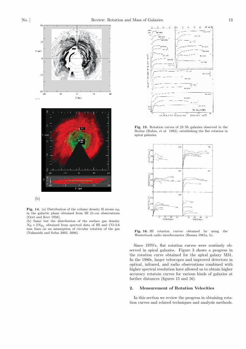
Fig. 14. (a) Distribution of the volume density H atoms nH

in the galactic plane obtained from HI 21-cm observations(Oort and Kerr 1958).(b) Same but the distribution of the surface gas densityNH + 2NH2 obtained from spectral data of HI and CO-2.6mm lines on an assumption of circular rotation of the gas(Nakanishi and Sofue 2003, 2006).

Fig. 15. Rotation curves of 23 Sb galaxies observed in theHαline (Rubin, et al. 1982), establishing the flat rotation inspiral galaxies.

Fig. 16. HI rotation curves obtained by using theWesterbook radio interferometer (Bosma 1981a, b).

Since 1970’s, flat rotation curves were routinely ob-served in spiral galaxies. Figure 3 shows a progress inthe rotation curve obtained for the spiral galaxy M31.In the 1980s, larger telescopes and improved detectors inoptical, infrared, and radio observations combined withhigher spectral resolution have allowed us to obtain higheraccuracy rotatoin curves for various kinds of galaxies atfarther distances (figures 15 and 16).

2. Measurement of Rotation Velocities

In this section we review the progress in obtaining rota-tion curves and related techniques and analysis methods.

14 Y. Sofue [Vol. ,

The content is based on our earlier review in Sofue andRubin (2001), while recent topics and particular progressare added. In table 3 we list the major papers in whichrotation curve data are available in machine-readable for-mats, or in figures and tables.

Rotation curves are the major tool to derive the massdistribution not only in the Milky Way but also in externalgalaxies. They are usually derived from Doppler velocitiesof optical and radio emission lines such as Hα, [NII], HIand CO emission lines. These interstellar lines originatefrom galactic disk components with low-velocity disper-sion, which allows us to neglect the pressure term in theequation of motion for calculating the mass distribution.

2.1. Optical Observations

Observations of optical emission lines such as Hαand[NII] lines sample population I objects, particularly HIIregions associated with star forming regions in the galac-tic disk. These objects have small velocity dispersion com-pared to the rotation velocity, which allows us to derivecircular velocities without suffering from relatively highvelocity components by polulation II stars. The tradi-tional method to derive rotation curves is long slit spectralobservation along the major axis of disk galaxies (Rubinet al. 1982, 1985; Mathewson et al. 1992; Amram et al.1994; Corradi et al. 1991; Courteau 1997; Sofue et al.1998).

On the other hand, absorption lines, showing high ve-locity dispersion and slower rotation, manifest kinemat-ics of population II stars composing spheroidal compo-nents and thick disk. Their line width is used to estimatethe pressure term of the equation of motion to derive theVirial mass. In this paper, however, we concentrate onlow velocity dispersion component for rotation velocities.

Methods to employ Fabry-Perot spectrographs offermeasurements of two dimensional velocity fields in diskgalaxies (Vaughan 1989; Vogel et al. 1993; Regan andVogel 1994; Weiner and Williams 1996; Garrido et al.2002, 2004; Kamphius et al. 2000; Vogel et al. 1993;Shetty et al. 2007). The velocity field includes informa-tion not only the global galactic rotation, but also non-circular stream motions due to spiral arms and bars.

Spectral observations in the infrared wavelengths, in-cluding the Paα and/or [Si VI] lines, and integral fieldanalysis technique are powerful tool to reveal kinematicsof dusty disks (Krabbe et al. 1997; Tecza et al. 2000).They are useful not only in the nuclear regions of spiralgalaxies, but also in such particular regions as mergerswith dust buried nuclei.

Rotation of outer disks of galaxies is crucial to derive themass in the dark halo, while observations are still scaresbecause of the faint and small numbers of emission re-gions. Not only bright HII regions, but also planetarynebulae and satellite galaxies are used as test particles fordetermining the mass distribution in outer regions.

The recent ”DiskMass” survey of disk galaxies for massdistribution and mass-to-luminosity ratio have obtainedthe largest sample of two-dimensional dynamical data ofspiral galaxies (Bershady et al. 2010a, 2010b; Martinsson

Fig. 17. Slit spectrum of the Hα 6563A and [NII] 6584Alines along the major axis of Sb galaxy NGC 4527 (Sofue etal. 1998)

Fig. 18. Hα Fabry-Perot velocity field and derived rotationcurve (Garrido e al. 2004).

No. ] Review: Rotation and Mass of Galaxies 15

Table 3. Large catalogues of rotation curves in the two decades

Authors‡ (year) Objects Distances Method Catalogue type†

Mathewson et al. (1992) 965 southern spirals <∼ 100 Mpc Hα/HI RC/TFAmram et al. (1992) 21 NGC/UGC Cluster Hα RC/VF/tab.Makarov et al. (1997, 2001) 135 edge-on ∼ 100 Mpc Hα RCFridman et al. (2005) 15 Sb/Sc/NGC 10 - 70 Mpc Hα/FP RC/PV/VFGHASP (2002-05) 85 spirals Hα/FP RC/VFMarquez et al. (2002) 111 spipral/NGC Hα/HII RCBlais-Ouellette et al. (2004) 6 Sb/Sc <∼ 20 Mpc FP RC/VFURC (1996-2007) Spirals Nearby Av. of compil. Universal RCNoordermeer et al. (2007) 19 S0/Sa/U,NGC 15 - 65 Mpc Hα/HI RC/PV/VFTHINGS (2008) 19 Nearby NGC Nearby HI RC/PV/VFSpano et al. (2008) 36 NGC Nearby HI RCDiskMass (2010-13) 146 face-on B < 14.7 Hα/[OIII]/CaII/IS RC/VFSofue et al. (1996); Sofue(2003, 2015b) ∼ 100 Sb/Sc/NGC Nearby+Virgo Hα/CO/HI RC/PV

McGaugh et al. (2001) 36 LSB Hα/slit RCde Blok and Bosma (2002) 26 LSB/UGC 3 - 45 Mpc Hα/HI RC/PVSwaters et al. (2009) 62 LSB dw/Ir/UGC Nearby Hα RC/PV

∗ http://www.ioa.s.u-tokyo.ac.jp/∼sofue/h-rot.htm. † RC=rotation curve, VF=velocity field, PV=position-velocitydiagram, FP=Fabry Perrot, IS=integral fiber spectroscopy. ‡ URC: Persic et al. (1996), Salucci et al. (2007);THINGS:de Blok et al. (2008); GHASP: Garrido et al. (2002-05); DiskMass: Bershady et al.(2010a,b), Martinsson et al.(2013a,b).

et al. 2013a, 2013b; Westfall et al. 2014). They employedintegral-field spectroscopy fiber instruments to measurestellar and ionized gas kinematics at multiple wavelengthsfrom 500 to 900 nm, covering [OIII]λ5007 and Hαin emis-sion, and MgIb and CaII near-infrared triplet in stellarabsorption. The observations were obtained for nearlyface-on galaxies selected from the UGC (Upsala GalaxiesCatalogue), including 146 nearly face-on galaxies brighterthan B = 14.7 and disk scale lengths between 10 and 20arcsec.

2.2. Radio Line Observations

The 21-cm HI line is powerful to obtain kinematics ofentire spiral galaxy because its radial extent is usuallymuch greater than that of the visible disk. HI measure-ments have played a fundamental role in establishing theflatness of rotation curves in spiral galaxies (e.g., Bosma1981a, b).

The rotational transition lines of CO molecules in themillimeter wave range are valuable in studying rotationkinematics of the inner disk and central regions of spiralgalaxies for their extinction free nature against the centraldusty disks (Sofue 1996, 1997). Also, the molecular gas isconcentrated in the central region , where HI is deficient(Sofue et al 1995; Honma et al. 1995), the CO line is agood alternative to HI and Hα.

Edge-on and high-inclination galaxies are particularlyuseful for rotation curve analysis in order to minimize theuncertainty arising from inclination corrections, for whichextinction-free measurements in radio lines are crucial, es-

pecially for central rotation curves.

3. Methods to Determine Rotation Velocities

A rotation curve of a galaxy is defined as the trace ofterminal velocities along the major axis, corrected for theinclination angle between the line-of-sight and the rotationaxis of the galaxy disk. The observed lines are an integralalong the line of sight through the galaxy. Hence, theintensity peaks do not necessarily represent the terminalvelocities.

3.1. Peak-Intensity and Intensity-Weighted VelocityMethods

In outer galactic disks, where line profiles can be as-sumed to be symmetric about the peak-intensity value,a velocity at which the intensity attains its maximum isoften used to represent the rotation velocity, which wecall the peak-intensity velocity method (Mathewson et al.1992, 1996).

A widely used method is to trace intensity-weighted ve-locities, which are also approximated by a centroid veloc-ity of half-maximum values of a line profile (Rubin et al.1982, 1985). The intensity-weighted velocity is defined by

Vint =∫

I(v)vdv/

∫I(v)dv, (42)

where I(v) is the intensity profile at a given radius as afunction of the radial velocity. Rotation velocity is thengiven by

16 Y. Sofue [Vol. ,

Fig. 19. Position-velocity diagram along the major axis ofthe edge-on galaxy NGC 3079. Dashed and central fullcontours are from HI (Irwin and Seaquist 1991) and CO(J = 1− 0) (Sofue et al. 2001) line observations, respectively.

Ve

locity (

arb

. u

nit)

Ve

locity (

arb

. u

nit)

Ve

locity (

arb

. u

nit)

Longitude (arb. unit)

Resolution

300

0

-300

300

0

-300

300

0

-300

-30 0 30

Fig. 20. [Top] A model rotation curve comprising a massivecore, bulge, disk and halo. Distributions of the molecular(CO) and HI gases are given by thin lines. [Middle] Composedposition-velocity diagram in CO, and [bottom] HI.

Vrot = (Vint −Vsys)/sin i, (43)

where i is the inclination angle and Vsys is the systemicvelocity of the galaxy. The centroid velocity is often ob-tained by tracing the values on the mean-velocity map ofa disk galaxy, which is usually produced from a spectraldata cube by taking the 1st moment.

However, it is largely deviated from the true rotationspeed in the innermost region, where the velocity struc-ture is complicated. It should be remembered that themean velocity near the nucleus gives always underesti-mated rotation velocity, because the finite resolution ofobservation inevitably results in zero value at the cen-ter by averaging plus and minus values in both sides ofnucleus along the major axis. Hence, the derived rota-tion curve often starts from zero velocity in the center.But the nucleus is the place where the stars and gases aremost violently moving, often nesting a black hole with thesurrounding objects moving at high-velocities close to thelight speed.

3.2. Terminal velocity method

This method makes use of the terminal velocity in aPV diagram along the major axis. The rotation velocityis derived by using the terminal velocity Vt:

Vrot = Vt/sin i − (Σ2obs +Σ2

ISM)1/2, (44)

where ΣISM and Σobs are the velocity dispersion of theinterstellar gas and the velocity resolution of observations,respectively. The interstellar velocity dispersion is of theorder of ΣISM ∼ 5 to 10 km s−1, while Σobs depends onthe instruments.

Here, the terminal velocity is defined by a velocity atwhich the intensity becomes equal to It = [(ηImax)2 +I2lc]

1/2 on the observed PV diagram, where Imax and Ilc

are the maximum intensity and intensity correspondingto the lowest contour level, respectively, and η is usuallytaken to be ∼ 0.2% so that the 20% level of the intensityprofile is traced. If the intensity is weak, the equationgives It ≃ Ilc which approximately defines the loci alongthe lowest contour level.

3.3. Envelope-Tracing Method

The terminal velocity Vt in a PV diagram is defined bya velocity at which the intensity is equal to

It = [(ηImax)2 + I2lc]

1/2, (45)

where Imax is the maximum intensity and Ilc is the inten-sity corresponding to the lowest contour level, often takenat ∼ 3 rms noise of the PV map. The fraction η (0.2∼ 0.5)represents the critical intensity level of the line profile.

The rotation velocity is derived using Ilc as

Vrot = (Vt −Vsys)/sin i − (σ2obs +σ2

ISM)1/2, (46)

where σISM and σobs are the velocity dispersion of theinterstellar gas and the velocity resolution of observations,respectively. The interstellar velocity dispersion is of theorder of σISM ∼ 7 to 10 km s−1, while σobs depends oninstruments.

No. ] Review: Rotation and Mass of Galaxies 17

Observed PV / Cube

Initial V(0) from PV

PV(i), Cube(i)

V(i), and dV(i)=V(0)-V(i)

Intensity distribution PV(r) / Cube(x,y)

V(i+1)=V(i)+dV(i)

V(i)=Rotation Curve

Sum dV(i)2 < Criterion

No

Yes

Fig. 21. Iteration method of rotation curve fitting using PVdiagrams and/or 3D cube.

3.4. Iteration methods using PV diagram and 3D cube

A more reliable method is to reproduce the observed PVdiagram by correcting the iteratively obtained rotationcurves (Takamiya and Sofue 2000). This method com-prises the following procedure. An initial rotation curveRC0 is obtained from the observed PV diagram by anymethod as above. Using RC0 and the observed radialdistribution of the intensity, a PV diagram, PV1, is con-structed. The difference between PV1 and PV0 is thenused to correct RC0 to obtain a corrected rotation curve,RC1. This RC is used to calculate another PV diagramPV2 using the observed intensity distribution, from whichthe next iterated rotation curve, RC2 is obtained by cor-recting for the difference between PV2 and PV0. This pro-cedure is iteratively repeated until PVi and PV0 becomesidentical within the error, and the final PVi is adopted asthe most reliable rotation curve.

This method, as well as the traditional methods de-scribed so far, utilizes only a portion of the kinematicaldata of a galaxy, e.g. a PV diagram along the major axisor a two-dimensional velocity field. The next-generationmethod to deduce rotation curve would be to utilize three-dimensional spectral data, or a spectral cube, from theentire galaxy. This may be particularly useful for radioline observations, since the lines are transparent at anyplaces in the disk.

The reduction procedure would be similar to that forthe iteration method: First, an approximate rotationcurve is given, and a spectral cube is calculated from thecurve based on the density distribution already derivedfrom the projected intensity distribution. Next, the cal-culated cube is compared with the observed cube to findthe difference. Then, the assumed rotation curve is itera-tively corrected so that the difference between the calcu-lated and observed cube is minimized.

X (arc sec)50 0 -50

200

0

-200

Vrot km/s

X (arc sec)50 0 -50

200

0

-200

Vrot km/s

X (arc sec)50 0 -50

200

0

-200

Vrot km/s

Fig. 22. Iteration method: a PV diagram of NGC 4536 inthe CO line (top panel), an approximate rotation curve usingthe peak-intensity method and corresponding PV diagram,the final rotation curve and reproduced PV diagram (bot-tom).

4. Tilted-ring Fitting Method using VelocityFields

4.1. Coupling of rotation velocity and inclination

The rotation velocity Vrot, inclination angle i, and ob-served radial velocity vr relative to the systemic velocityare related to each other as

vr(r,θ) = Vrot(r) cos θ sin i, (47)

where θ is azimuth angle in the disk of a measured pointfrom the major axis. Obviously the rotation velocity andinclination are coupled to yield the same value of vr.

The most convenient way to derive a rotation curve isto measure radial velocities along the major axis usingposition-velocity diagrams, as described in the previoussubsection. Thereby, inclination angle i has to be mea-sured independently or assumed. Given the inclination,the rotation velocity is obtained by

Vrot =vr

sin i(48)

with vr = vr(r,0).

18 Y. Sofue [Vol. ,

Inclination angle is usually measured from the major-to-minor axial ratio of isophotal ellipses on optical images.An alternative way is to compare the integrated HI linewidth with that expected from the Tully-Fisher relation(Shetty et al. 2007). However, equation 48 trivially showsthat the error in resulting velocity is large for small i, andthe result even diverges for a face-on galaxy with i ∼ 0.

4.2. Tilted-ring method: Simultaneous determination ofrotation velocity and inclination

If a velocity field is observed, coupling of rotation ve-locity and inclination can be solved using the tilted-ringtechnique (Bosma 1981; Begeman 1989; Jozsa et al. 2007).This method utilizes the unique dependence of the varia-tion of radial-velocity against ϕ upon the inclination anglei. Radial velocity vr is related to position angle ϕ and az-imuthal angle θ as

f(θ, i) =vr

vr,max= cos θ(ϕ,i), (49)

with

θ(ϕ,i) = atan(

tan ϕ

cos i

), (50)

and vr,max is the maximum value along an annulus ring.Figure 24 shows variations of cos θ(ϕ), or vr normalized

by its maximum value along an annulus ring, as functionsof ϕ and θ for different values of inclination. The func-tional shape against ϕ is uniquely dependent on inclina-tion i, which makes it possible to determine inclinationangle by iterative fitting of vr by the function. Once i isdetermined, Vrot is calculated using vr. Thus, both theinclination and Vrot are obtained simultaneously.

In often adopted method, the galactic disk is dividedinto many oval rings, whose position angles of major axisare determined by tracing the maximum saddle loci ofthe velocity field. Along each ring the angle θ is mea-sured from the major axis. Observed values of f(θ, i) arecompared with calculated values, and the value of i is ad-justed until chi2 gets minimal stable. The value of i yield-ing the least χ2 is adopted as the inclination of this ring.This procedure is applied to neighboring rings iterativelyto yield the least χ2 over all the rings. Di Teodoro andFraternali (2015) recently developed a more sophisticatedmethod incorporating the velocity field as a 3D cube data(velocity, x and y) to fit to a disk rotation curve.

This method is effective for highly inclined galaxies withlarge i, while the functional shapes become less sensi-tive to i in face-on galaxies, resulting in poorer accuracy.Begeman (1989) has extensively studied the tilted-ringmethod, and concluded that it is not possible to deter-mine inclinations for galaxies whose inclination angles areless than 40.

4.3. Inclination determination using assumed rotationvelocity

Equation 48 is rewritten as sin i=vr/Vrot, which meansthat the inclination can be determined by measuring vr,if Vrot is given. This principle is used in determination

20 40 60 80phi, theta deg.

0.2

0.4

0.6

0.8

1

V’

Fig. 23. Variation of V ′ = vr/vr,max along a tilted-ring as afunction of position angle ϕ (full line) for different inclinations(from bottom lines: i = 85, 75, 60, 45, 30 and 15).Variation against azimuthal angle θ is shown dashed.

Fig. 24. Tilted rings and velocity field fitted to HI velocityfields of NGC 5055 (Bosma 1981a).

of inclination using the Tully-Fisher relation, where oneestimates an intrinsic line width using the disk luminosity,and compares it with observed line width to get inclina-tion angle. Shetty et al. (2007) obtained i = 24 usingthis method. The above equation can also be applied toindividual annulus rings, if the rotation curve is assumed.It is obvious that the accuracy of determination of i ishigher for more face-on galaxies. This method was in-deed applied to mesure warping of the outer HI disk ofthe face-on galaxy NGC 628 (Kamphuis and Briggs 1992)and M51 (Oikawa and Sofue 2014).

To summarize, the 1st and 2nd methods, which are thepopular method to derive rotation curve assuming incli-nation and the tilted-ring method, are useful for largelyinclined galaxies with i > 30−40, but they failed in moreface-on galaxies. On the other hand, the 2nd method, amethod to determine inclination assuming rotation curve,is useful to study inclinations in a warped disk in face-ongalaxies.

No. ] Review: Rotation and Mass of Galaxies 19

(1) (2) (3)

(4) (5) (6)

(7) (8) (9)

(10)

Fig. 26. Rotation curves compiled and reproduced from the literature. References are in the order of panel numbers, (1) Sofue etal. (1999): Nearby galaxy rotation curve atlas; (2) Sofue et al. (2003): Virgo galaxy CO line survey; (3) Sofue et al. (1999: NGC253 revised); Ryder et al. (1998, NGC157); Hlavacek-Larrondo et al. (2011a: NGC253; 2011b: NGC 300); Erroz-Ferrer et al. (2012:NGC 864); Gentile et al. (2015: NGC 3223); Olling R. P. (1996: NGC 4244); Whitmore & Schweizer (1987: NGC 4650A); Gentileet al. (2007: NGC 6907); (4) Marquez et al. (2004): Isolated galaxy survey; (5) de Blok et al. (2008): THINGS survey, wheredashed galaxies are included in (1) and were not used in the analysis; (6) Garrido et al. (2005): GHASP survey; (7) Noordermeeret al. (2007): Early type spiral survey; (8) Swaters et al. (2009): Dwarf and low-surface-brightness galaxy survey; (9) Martinssonet al. (2013): DiskMass survey; and (10) All rotation curves in one panel.

20 Y. Sofue [Vol. ,

Fig. 25. Rotation curve derived from HI velocity fields usingthe tilted ring method (de Blok et al 2008).

R / h

Vrot

(km/s)

0 1 2 3 4 5

100

200

300

400

Fig. 27. Rotation curves of spiral galaxies plotted againstradius normalized by the scale length h.

5. Galaxy Types and Rotation Curves

5.1. Observed rotation curves

Figure 26 shows rotation curves published in the twodecades as compiled from the literature by Sofue (2015b).

Fig. 27 shows more recently compiled rotation curvesobserved in nearby spiral galaxies, which have been ob-tained by optical, CO and HI line data (Sofue et al. 1999).Fig. 29 shows rotation curves for individual galaxies typesfrom Sa to Sc.

It is remarkable that the form, but not amplitude, of thedisk and halo rotation curves is similar to each other fordifferent morphologies from Sa to Sc, from less massiveto massive galaxies. This suggests that the form of thegravitational potential in the disk and halo is not stronglydependent on the galaxy type.

Figure 27 shows examples of rotation curves of nearbyspiral galaxies obtained by combining optical (mainly Hα)and radio (CO and HI) observations, where the circularvelocity is plotted against linear radius and in terms ofscale radius h (Sofue et al. 1999).

There is a marked similarity of form of rotation curves

(a)5 10 15 20 25 30

R kpc

50

100

150

200

250

300

350

400

Vro

tkms

Central Peak

(b)5 10 15 20 25 30

R kpc

50

100

150

200

250

300

350

400

Vro

tkms

No Central Peak

(c)5 10 15 20 25 30

R kpc

50

100

150

200

250

300

350

400

Vro

tkms

Rigid-Body Rise

Fig. 28. Classification of rotation curve shapes. [a] Centrallypeaked type, [b] shoulder rise type, and [c] rigid-body rise type(Sofue et al. 1999).

for galaxies with different morphologies from Sa to Sc (fig-ure 27). The forms may be classified into three groups: thecentrally peaked, shoulder rise, and rigid-body rise types(figure 28. The three types are observed mainly in mas-sive and large-diameter galaxies, medium sized galaxies,and less massive Sc and dwarf galaxies, respectively.

5.2. Universal rotation curve

Massive galaxies show a steeper rise and higher centralvelocities within a few hundred pc of the nucleus comparedto less massive Sc galaxies (figure 30). On the contrary,dwarf galaxies generally show a gentle central rise in arigid-body fashion. The most massive galaxies have flat orslightly declining rotation in the outmost part, while lessluminous galaxies show rigid-body rise and monotonicallyincreasing outer rotation curve (Persic et al. 1996).

There have been several attempts to represent the ob-served rotation curves by simple functions (Persic et al.1996; Courteau 1997; Roscoe 1999). Persic et al. (1996)fit the curves by a formula, which is a function of to-tal luminosity and radius, comprising both disk and halocomponents. Both the forms and amplitudes are functionsof the luminosity, and the outer gradient of the RC is adecreasing function of luminosity (figure 30).

5.3. Galaxy types and RC shape

The differences in the curve shapes are related to thebulge-to-disk mass ratio: the smaller is the ratio, andtherefore, the later is the galaxy type, the milder is thecentral rise, although the correspondence is not necessar-ily unique. The individuality of the rotation curve form

No. ] Review: Rotation and Mass of Galaxies 21

R (kpc)

V

(km/s)

Sa galaxies

0 10 20 30

100

200

300

400

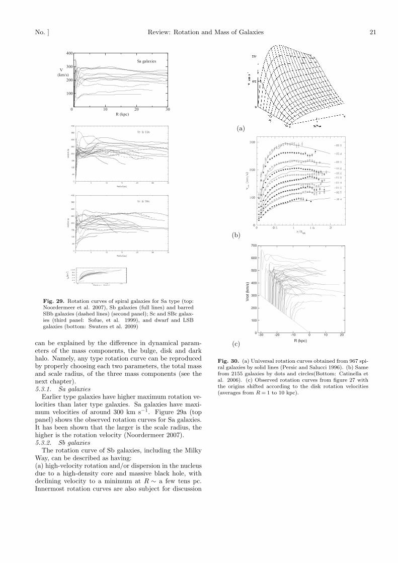
Fig. 29. Rotation curves of spiral galaxies for Sa type (top:Noordermeer et al. 2007), Sb galaxies (full lines) and barredSBb galaxies (dashed lines) (second panel); Sc and SBc galax-ies (third panel: Sofue, et al. 1999), and dwarf and LSBgalaxies (bottom: Swaters et al. 2009)

can be explained by the difference in dynamical param-eters of the mass components, the bulge, disk and darkhalo. Namely, any type rotation curve can be reproducedby properly choosing each two parameters, the total massand scale radius, of the three mass components (see thenext chapter).5.3.1. Sa galaxies

Earlier type galaxies have higher maximum rotation ve-locities than later type galaxies. Sa galaxies have maxi-mum velocities of around 300 km s−1. Figure 29a (toppanel) shows the observed rotation curves for Sa galaxies.It has been shown that the larger is the scale radius, thehigher is the rotation velocity (Noordermeer 2007).5.3.2. Sb galaxies

The rotation curve of Sb galaxies, including the MilkyWay, can be described as having:(a) high-velocity rotation and/or dispersion in the nucleusdue to a high-density core and massive black hole, withdeclining velocity to a minimum at R ∼ a few tens pc.Innermost rotation curves are also subject for discussion

(a)

(b)

(c) R (kpc)

Vrot(km/s)

-30 -20 -10 0 10 200

100

200

300

400

500

600

700

Fig. 30. (a) Universal rotation curves obtained from 967 spi-ral galaxies by solid lines (Persic and Salucci 1996). (b) Samefrom 2155 galaxies by dots and circles(Bottom: Catinella etal. 2006). (c) Observed rotation curves from figure 27 withthe origins shifted according to the disk rotation velocities(averages from R = 1 to 10 kpc).

22 Y. Sofue [Vol. ,

Fig. 31. Black circles show Gaussian averaged rotation curvefrom all galaxies listed in Sofue et al. (1999). Long and shortbars are standard deviations and standard errors, respec-tively. Thin lines show the least-χ2 fitting by de Vaucouleursbulge (scale radius 0.57 kpc, mass 9.4×109M⊙), exponentialdisk (2.7 kpc, 3.5× 1010M⊙), and NFW dark halo (35 kpc,ρ0 =3×10−3M⊙pc−3). Three dashed lines are averaged rota-tion curves of galaxies with maximum velocities greater than200 km s−1, between 200 and 250 km s−1, and below 200 kms−1, respectively, from top to bottom.

of central bars and non-circular motions which may besuperposed on the rotation. ;(b) steep rise of RC within the central 100 pc due to thecore of bulge;(c) maximum at radius of a few hundred pc due to thebulge, followed by a decline to a minimum at 1 to 2 kpc;then,(d) gradual rise to the maximum at 5 to 7 kpc due to thedisk; and(e) nearly flat outer rotation due to the dark halo up toR ∼ 20− 30 kpc.5.3.3. Sc galaxies

Sc galaxies have lower maximum velocities than Sa andSb, ranging from ≤ 100 to ∼ 200 km s−1with the me-dian value of 175 km s−1(Rubin et al. 1985). Massive Scgalaxies show a steep nuclear rise similar to Sb’s, whileless-massive Sc galaxies have gentler rise. They also havea flat rotation to their outer edges. Less luminous (lowersurface brightness) Sc galaxies have a gentle central riseof rotation velocity, which monotonically increases till theouter edge. This behavior is similar to rotation curves ofdwarf galaxies.

5.4. Flatness and similarity of rotation curves

The flatness of the overall shape of entire rotationcurves applies to any mass ranges of galaxies. Figure 31shows averaged rotation curves of galaxies from the sam-ple of Sofue et al (1999), categorized into three groups bydashed lines, one those with maximum rotation velocitygreater than 250 km s−1, and the second between 200 and250 km s−1, and the third slower than 200 km s−1.

The thick line shows a Gaussian averaged rotation curveof all the sample galaxies, where long and short bars de-note the standard deviation and standard error of themean value, respectively, in each radius bin at 0.5 kpcinterval with Gaussian averaging width of 0.5 kpc.

5.5. Barred Galaxies

Rotation properties of SBb and SBc galaxies are gener-ally similar to those of non-barred galaxies of Sb and Sctypes. However, their kinematics is more complicated dueto the non-circular streaming motion by the oval poten-tial, which results in skewed velocity fields and ripples onthe rotation curves (e.g., Bosma 1981a,1996).

CO and optical line mapping and spectroscopy re-veal high concentration of molecular gas in shocked lanesalong a bar superposed by significant non-circular mo-tions. They show strong non-circular streaming motion,and often velocity jumps of ∼ 50− 100 km s−1(Kuno etal. 2000; Hunter and Gottesman 1996; Buta et al. 1999).CO line velocities manifest the velocity of shocked gas,and therefore, observed velocities are close to those of gasin rigid-body motion with a bar, slower than the circularvelocity. This results in underestimated rotation veloc-ities. Geometrical effect that the probability of side-onview of a bar is greater than that of end-on view alsocauses statistically underestimated rotation velocities.

Thus, not only because of the large number of param-eters for a barred galaxy as listed in table 1, but alsofor the above reasons, quantifying the bar is not uniquelyobtained from the current limited velocity information

5.6. Dwarf and Low Surface Brightness (LSB) Galaxies

Within the two decades, a large number of low surfacebrightness (LSB) galaxies have been found (Schombertand Bothun 1988; Schombert et al. 1992). Dwarf and LSBgalaxies show slow rotation at ≤ 100 km s−1with mono-tonically rising rotation velocity until their last measuredpoints (de Blok et al. 1996, 2001; de Blok 2005; Swaters etal. 2000, 2001, 2009; Carignan and Freeman 1985; Blais-Quellette et al. 2001; Noordermeer et al. 2009; figure 29).Blue compact galaxies also show that rotation curves risemonotonically to the edges of the galaxies (Ostlin et al.1999). Also, dwarfs with higher central light concentra-tions have more steeply rising rotation curves, similarlyto spirals.

The mass-to-luminosity ratio of dwarfs and LSB is usu-ally higher than that for normal spirals, and the darkmatter fraction is much higher (Carignan 1985; Jobin andCarignan 1990; Carignan and Freeman 1985; Carignanand Puche 1990a,b; Carignan and Beaulieu 1989; Pucheet al. 1990, 1991a, b; Lake et al. 1990; Broeils 1992;Blais-Ouellette et al. 2001; Carignan et al. 2006).

5.7. Interacting and irregular galaxies

The Large Magellanic Cloud (LMC) is the nearest dwarfgalaxy interacting with the Milky Way. Despite of the in-teraction, a flat rotation curve from the dynamical centerto the outer edge at R ∼ 5 kpc at a velocity ∼ 100 kms−1(Kime et al. 1998). The rotation curve has a steep cen-tral rise, followed by a flat rotation. The dynamical centerinferred from the velocity field is significantly displacedfrom the optical bar center, indicating the existence of amassive component that is not visible as a stellar bulge.The “dark bulge” has a significant mass as dark matter,

No. ] Review: Rotation and Mass of Galaxies 23

R (kpc)

Vrot(km/s)

0 5 10 15 20 25 30-300

-200

-100

0

100

200

300

X kpc

Y k

pc

-30 -20 -10 0 10 20 30

-10

0

10

Fig. 32. [Top] Anomalous rotation curve of M51 showingfaster decrease than Keplerian beyond 8 kpc followed byapparent counter rotation, compared with averaged rota-tion curve of spiral galaxies. [Bottom] Warped disk calcu-lated for rotation curve assuming a universal rotation. Theline-of-sight is toward top. (Oikawa and Sofue 2014)

showing an anomalously high mass-to-luminosity (M/L)ratio around the dynamical center (Sofue 1999). However,the stellar bar has a smaller M/L ratio compared to thatof the surrounding regions.

Rotation curves for irregular and interacting galaxiesare not straightforward. Some irregular galaxies exhibitquite normal rotation curves, whereas some reveal appar-ently peculiar rotations. Hence, it is difficult to deduce ageneral law property to describe the curves, but individ-ual cases may be studied in case by case. We may raisesome examples below.

The typical interacting galaxy NGC 5194 (M51) showsa rotation curve, which declines more rapidly thanKeplerian in the outer disk (figure 32). Even counter ro-tation is observed in the outermost HI ring (Rots et al.1990; Appleton et al. 1986). Kinematics of M51 has beenobserved at various wavelengths, which all indicates therotation anomaly. The rotation anomaly is explained bythe warping of galactic disk, assuming that the galaxy hasintrinsically normal flat rotation curve (Oikawa and Sofue2014). Figure 32 shows a calculated warping of the diskfor a given normal rotation curve, where the disk is nearlyflat and then bends at r = 7.5 kpc steeply.

The starburst dwarf galaxy NGC 3034 (M82) is a com-panion to the giant spiral M81, and shows an exceptionallypeculiar rotation property. It has a normal steep nuclearrise and rotation velocities which have a Keplerian declinebeyond the nuclear peak. This may arise from a tidal trun-cation of the disk and/or halo by an encounter with M81(Sofue 1992).

V(km/s)

R (kpc)

0.0001 0.001 0.01 0.1 1 10 10010

100

Fig. 33. Logarithmic rotation curves of nearby spiral galax-ies with typical resolutions, ∼ 2− 10′′ (thick lines) and thosefrom Virgo CO survey (∼ 1′′, thick dashed lines), comparedwith the Milky Way rotation curve (circles with error bars).Thin dashed lines show NGC 224, 1068 and 4258 as interpo-lated with their black holes by horizontal straight lines.

6. Central Rotation Curves

Central rotation curves have been produced for a num-ber of galaxies by a systematic compilation of PV dia-grams in the CO and Hα lines (Sofue 1996; Sofue etal. 1997, 1998, 1999). Bertola et al. (1998) have em-phasized that the high-velocity nuclear peaks observed insome spiral galaxies match the simulated PV diagrams forKeplerian rotation due to a massive black hole.

Many spirals exhibits rapid central velocities, offeringevidence for massive nuclear black holes (van der Marel etal. 1994; Miyoshi et al. 1995; Kormendy and Richstone1995; Richstone, et al. 1998, Bertola et al. 1998; Ferrarese1999; Kormendy and Westpfahl 1989; Kormendy 2001).In NGC 4258, water masers at 22 GHz are observed froma disk of radius 0.1 pc in Keplerian rotation, indicating theexistence of a massive black hole of mass of 3.9× 107M⊙(Nakai et al. 1993; Watson and Wallim 1994; Miyoshiet al. 1995; Herrnstein et al. 1999). VLBI observationsof the water maser line have revealed a rapidly rotatingnuclear torus of sub parsec scales in several nearby activegalactic nuclei (Haschick et al. 1990; Trotter et al. 1998;Sawada-Satoh et al. 2000; Greenhill et al. 1996).

Logarithmic presentation of rotation curves is powerfulto discuss the innermost dynamics in relation to the galac-tic structure. Figure 33 shows rotation curves of nearbygalaxies and Virgo samples in logarithmic presentation.Also shown are the rotation curves of nearby galaxieswith known super massive black hole, where black holesand outer rotation curves are interpolated by dashed lines.The thick line with dots and error bars are the rotationcurve of the Milky Way (Sofue 2013b). The figure demon-strates that, except for the Milky Way, the resolution isnot sufficient, and higher resolution observations such asusing ALMA are a promising subject for the future forlinking the central black hole to the galactic structure.

Simulation in figure 22 reveals the effect of the finiteresolution on the observed PV diagram as shown. Centralrotation curves derived from observed PV diagrams gener-ally give lower limits to the rotation velocities. The angu-lar resolution is crucial for the analysis of central dynamics

24 Y. Sofue [Vol. ,

R (kpc)

V(km/s)

0.1 1 10 100

100

8090

200

300

400

Fig. 34. Grand rotation curve of M31. Thin lines show theleast-χ2 fit by the bulge, disk and dark halo components.

together with high dynamic range and precise subtractionof bulge continuum light (e.g., Rubin et al. 1997; Sofue etal. 1998, 1999a; Bertola et al. 1998). However, interstellarextinction is strongest in optical observations. To avoidthis difficulty, radio line observations, particularly the COlines, are crucial because of the negligible extinction andhigh density concentration in the nuclei (e.g., Sofue et al.1999a).

6.1. Activity and Rotation Curves

High-accuracy central rotation curves for starburstgalaxies, Seyferts, LINERs, and galaxies with nuclear jetsshow no particular peculiarity (Sofue et al. 1999a). Evensuch a very active galaxy like NGC 5128 (Cen A) showsa rotation curve much like a normal galaxy (van Gorkomet al. 1990). The radio lobe galaxy NGC 3079 has strongnuclear activity, but shows usual rotation properties withvery high central velocities (Sofue and Irwin 1992; Irwinand Sofue 1992).

While these galaxies all show a very steep central ve-locity rise, such steep rise is not peculiar but generallyobserved for massive galaxies without pronounced centralactivity. Because the global rotation and mass distribu-tion in active spirals are thus normal, nuclear activity maynot be due to general dynamical structure, but is due totemporal causes around central deep gravitational poten-tial triggered by some intermittent feeding of circum nu-clear gas and stars.

7. Dark Halo: Grand Rotation Curves

The outermost rotation curve beyond the flat disk is stillnot well determined for external galaxies because of thelack in extended disk and weak emissions. In order to solvethis difficulty, non-coplanar objects such as outer globularclusters and satellite galaxies have been often used to es-timate the dark halo masses applying the Virial theorem.

In order to derive mass distributions in dark halos ofnearby galaxies, grand rotation curves (GRC) have beenobtained, which represent expected (or pseudo) circularrotation velocities within several hundred kpc of the galax-ies (Sofue 2013b, 2015a). The technique has been appliedto M31 and the Milky Way to derive GRCs within ∼ 300kpc by combining disk rotation velocities and radial ve-locities of satellite galaxies and globular clusters. Figure

Fig. 35. Enclosed mass within R25 plotted against infraredabsolute luminosity in H band (Rubin et al. 1991)

(a)

(b)

(c)

Fig. 36. 2µ infrared Tully-Fisher relation (Masters et al.2008)

34 shows the GRCs and results of model fitting by bulge,disk and dark halo components (Sofue 2015a).

The GRC for the Milky Way presented here has beenrevised using the most recent Solar rotation velocity ofV0 = 238 km s−1from VERA observations (Honma et al.2013), revealing higher velocities in the outer regions com-pare to those shown in figures 10 and 39.

The GRCs were deconvolved into a de Vaucouleursbulge, exponential disk, and a dark halo with the Navarro-Frenk-White (1995: NFW) density profile by the leastχ squares fitting. Comparison of the best-fit parametersreveals a remarkable similarity of M31 and the Galaxy,except for the dark halo mass of M31 being twice theGalaxy’s. It may be emphasized that the NFW modelcan represent the observed dark halos in a sufficient accu-racy.

8. Statistical Properties of Rotation Curves:Tully-Fisher Relation

Rubin et al. (1985) used their synthetic rotation curvesto derive dynamical masses interior to the Holmberg ra-dius (R25) of spiral galaxies, and showed a clear corre-lation with the H-band infrared luminosity, as shown infigure 35. Instead of the total dynamical mass, the maxi-mum rotation velocity at a few galactic-disk scale radii wasshown to be related to the luminosity, as observed as one-half the velocity width of an integrated 21 cm HI line ve-locity profile. The relation is known as the Tully-Fisher re-lation (Tully and Fihser 1977; Aaronson and Mould 1986;

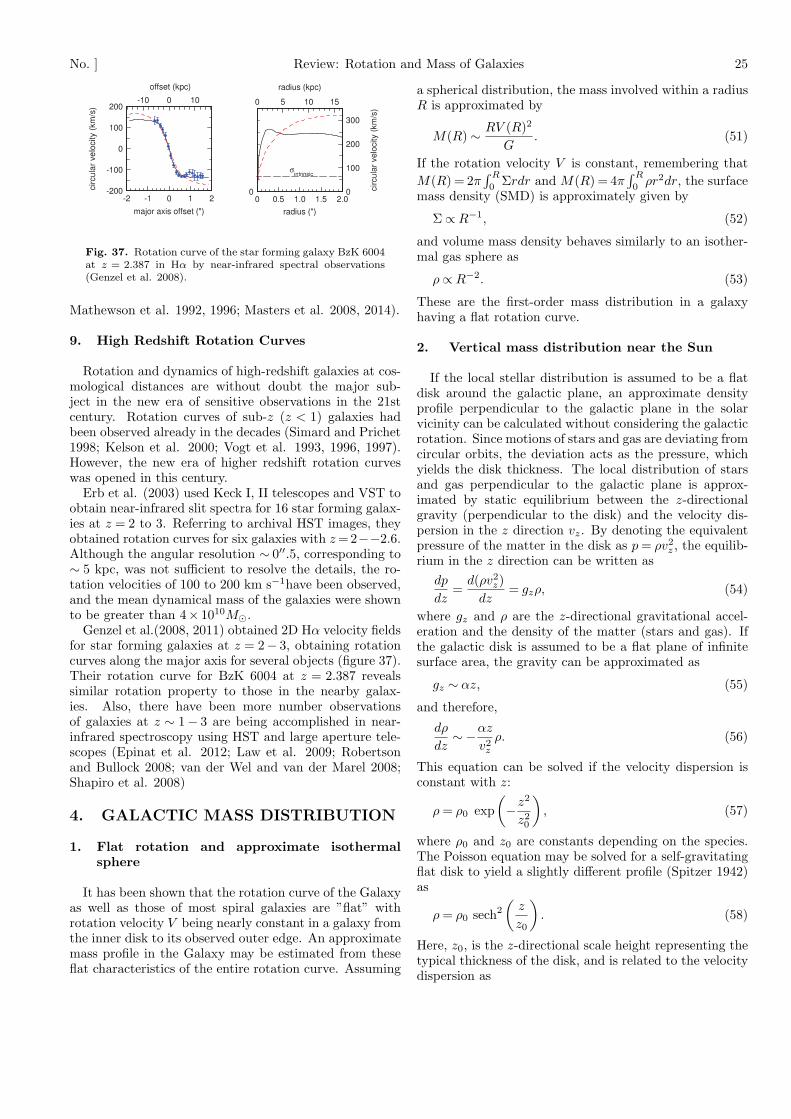
No. ] Review: Rotation and Mass of Galaxies 25

Fig. 37. Rotation curve of the star forming galaxy BzK 6004at z = 2.387 in Hα by near-infrared spectral observations(Genzel et al. 2008).

Mathewson et al. 1992, 1996; Masters et al. 2008, 2014).

9. High Redshift Rotation Curves

Rotation and dynamics of high-redshift galaxies at cos-mological distances are without doubt the major sub-ject in the new era of sensitive observations in the 21stcentury. Rotation curves of sub-z (z < 1) galaxies hadbeen observed already in the decades (Simard and Prichet1998; Kelson et al. 2000; Vogt et al. 1993, 1996, 1997).However, the new era of higher redshift rotation curveswas opened in this century.

Erb et al. (2003) used Keck I, II telescopes and VST toobtain near-infrared slit spectra for 16 star forming galax-ies at z = 2 to 3. Referring to archival HST images, theyobtained rotation curves for six galaxies with z =2−−2.6.Although the angular resolution ∼ 0′′.5, corresponding to∼ 5 kpc, was not sufficient to resolve the details, the ro-tation velocities of 100 to 200 km s−1have been observed,and the mean dynamical mass of the galaxies were shownto be greater than 4× 1010M⊙.

Genzel et al.(2008, 2011) obtained 2D Hα velocity fieldsfor star forming galaxies at z = 2− 3, obtaining rotationcurves along the major axis for several objects (figure 37).Their rotation curve for BzK 6004 at z = 2.387 revealssimilar rotation property to those in the nearby galax-ies. Also, there have been more number observationsof galaxies at z ∼ 1− 3 are being accomplished in near-infrared spectroscopy using HST and large aperture tele-scopes (Epinat et al. 2012; Law et al. 2009; Robertsonand Bullock 2008; van der Wel and van der Marel 2008;Shapiro et al. 2008)

4. GALACTIC MASS DISTRIBUTION

1. Flat rotation and approximate isothermalsphere

It has been shown that the rotation curve of the Galaxyas well as those of most spiral galaxies are ”flat” withrotation velocity V being nearly constant in a galaxy fromthe inner disk to its observed outer edge. An approximatemass profile in the Galaxy may be estimated from theseflat characteristics of the entire rotation curve. Assuming

a spherical distribution, the mass involved within a radiusR is approximated by

M(R) ∼ RV (R)2

G. (51)

If the rotation velocity V is constant, remembering thatM(R) = 2π

∫ R

0Σrdr and M(R) = 4π

∫ R

0ρr2dr, the surface

mass density (SMD) is approximately given by

Σ ∝ R−1, (52)

and volume mass density behaves similarly to an isother-mal gas sphere as

ρ ∝ R−2. (53)

These are the first-order mass distribution in a galaxyhaving a flat rotation curve.

2. Vertical mass distribution near the Sun

If the local stellar distribution is assumed to be a flatdisk around the galactic plane, an approximate densityprofile perpendicular to the galactic plane in the solarvicinity can be calculated without considering the galacticrotation. Since motions of stars and gas are deviating fromcircular orbits, the deviation acts as the pressure, whichyields the disk thickness. The local distribution of starsand gas perpendicular to the galactic plane is approx-imated by static equilibrium between the z-directionalgravity (perpendicular to the disk) and the velocity dis-persion in the z direction vz. By denoting the equivalentpressure of the matter in the disk as p = ρv2

z , the equilib-rium in the z direction can be written as

dp

dz=

d(ρv2z)

dz= gzρ, (54)

where gz and ρ are the z-directional gravitational accel-eration and the density of the matter (stars and gas). Ifthe galactic disk is assumed to be a flat plane of infinitesurface area, the gravity can be approximated as

gz ∼ αz, (55)

and therefore,

dρ

dz∼−αz

v2z

ρ. (56)

This equation can be solved if the velocity dispersion isconstant with z:

ρ = ρ0 exp(−z2

z20

), (57)

where ρ0 and z0 are constants depending on the species.The Poisson equation may be solved for a self-gravitatingflat disk to yield a slightly different profile (Spitzer 1942)as

ρ = ρ0 sech2

(z

z0

). (58)

Here, z0, is the z-directional scale height representing thetypical thickness of the disk, and is related to the velocitydispersion as

26 Y. Sofue [Vol. ,

-4 -2 0 2 4z normalized by z_0

0.2

0.4

0.6

0.8

1

rho

norm

aliz

edby

rho_

0

Mass density profile perpendicular to the disk

Fig. 38. Mass density profile perpendicular to the local disk.The solid curve represents the Gaussian profile for a hydro-static disk, and the dashed line is for a self-gravitating disk.

z0 =vz√α∼√

k

αmHTgas. (59)

In figure 38 the two results from equation (57) and (58)are compared. Table 4 summarizes the typical valuesof vz and the disk scale-thickness z0 for various species.Population I objects are distributed in a disk of thick-ness 2z0 ∼ 100 pc, and Population II stars in a disk withthickness 2z0 ∼ 300 pc.

Component vz (km s−1) 2z0 (pc)Molecular clouds 5 60OB stars 5 60HI gas 10 100Disk stars 20-30 300

Hot gas (106K) 100 (∼√

kTmH

) ∼ 2000

Table 4. Velocity dispersion in the z direction and scale ful-l-width thickness of the disk.

3. Decomposition into central core, bulge, diskand dark halo by the least χ2 fitting

The observed rotation curve is used to derive the massdistribution in the Galaxy. There are two ways to derivethe mass distribution from the rotation curve. One wayis to assume several mass components such as disk, and adark halo, and fit the rotation curve by calculated circularvelocities. The rotation velocity V (R) is represented by acombination of representing velocities of the componentsas

V (R) =√

ΣV 2i ≃

√Vb(R)2 +Vd(R)2 +Vh(R)2. (60)

If the resolution in the central region is sufficiently high,a more central component such as a black hole such asVBH(R)2 may be added to the right-hand side. Here, Vi

indicates circular velocity corresponding to the i-th com-ponent alone, and suffices BH, b, d and h denote a blackhole, bulge, disk, and halo components, respectively. Forthe fitting, the parameters such as the mass and scaleradius of individual components are adjusted so that theresidual between the calculation and observation gets min-imized.

The fitting is usually started from the inner component.First, the innermost steep rise and peak of the rotationcurve is fitted by a bulge component; second, the gradualrise and flat part is fitted by the disk, and finally, theresidual outskirt is fitted by a dark halo. Alternatively,these fittings may be done at the same time by givingapproximate parameters, which are adjusted iterativelyuntil the entire curve is best fitted.

The rotation curve of the Milky Way shows clearlythree dominant components: the galactic bulge peakingat R ∼ 300 pc, disk broadly peaking at R ∼ 6 kpc, andouter flat part due to the dark halo till the outer edge.The black hole does not contribute so much in the plottedscale, and may be treated as an independent object in thevery central region within ∼ 1 pc. These characteristicsare commonly observed in most of external disk galax-ies, and may be considered to be the universal property.Rotation curves, and therefore the mass distributions, inany galaxies including the Milky Way are, thus, similar toeach other. Hence, the same functional forms used for theGalaxy may be applied to any other galaxies, and viceversa, by modifying the parameters such as the massesand scale radii of individual components. Decompositionof a rotation curve into several mass components such asa bulge, disk and dark halo has been extensively appliedto observed data (Bosma 1981a; Kent 1986; Sofue 1996).

There are various functional forms to represent the masscomponents. The commonly employed mass profiles are:(i) de Vaucouleurs bulge + exponential disk: It is wellestablished that the luminosity profile of the spheroidalbulge component in galaxies is represented by the deVaucouleurs (e−(r/re)1/4

; 1958) or Sersic (e−(r/re)n

; 1958)law. The disk component is represented by the exponen-tial law (e−r/re (n = 1); Freeman 1970). For the halo,either isothermal, Navaro-Frenk-White, or Burkert profileare adopted.(ii) Miyamoto-Nagai potential: Another way is to assumea modified Plummer type potential for each component,and the most convenient profile is given by the Miyamoto-Nagai (1975) potential.

After fitting the rotation curve by the bulge, exponen-tial disk, and a dark halo, smaller structures superposedon the rotation curves are discussed as due to more localstructures such as spiral arms and/or bar.

4. Massive central component and Black Hole

The central rotation curve of the Galaxy indicates thatthe main bulge component has a velocity peak at r ≃400pc with V = 250 km s−1. It declines toward the centersteeply, followed by a plataeu-like hump at r ∼ 30− 3 pc.The plateau-like hump is then merged by the Keplerianrotation curve corresponding to the central black hole atr <∼ 2 pc. Here we use a black hole mass of MBH =4×106M⊙, taking the mean of the recent values convertedto the case for R0 =8.0 kpc, i.e., 2.6−4.4×106M⊙ (Genzelet al. 2000, 2010), 4.1− 4.3× 106M⊙ (Ghez et al. 2005),and 3.95× 106M⊙ (Gillessen et al. 2009).

For many spirals, including the Milky Way, the inner-

No. ] Review: Rotation and Mass of Galaxies 27

R (kpc)

V(km/s)

0.001 0.01 0.1 1 10 100 1000

100

50

60708090

200

300

400

Fig. 39. Logarithmic rotation curve of the Galaxy forV0 = 238 km s−1and deconvolution into a central black hole,two exponential-spherical bulges, exponential flat disk, andNFW dark halo by the least χ2 fitting shown by thin lines.A classical de Vaucouleurs bulge shown by the dashed line issignificantly displaced from the observation.

most region exhibits rapid rotation velocities, offering ev-idence for massive nuclear black holes. Consequently, or-bital velocities in the center decrease rapidly from a veloc-ity close to the speed of light down to 100 to 200 km s−1ofthe bulge and disk rotation velocities.. It has been estab-lished that the spheroidal component, e.g. bulge, is deeplycoupled with the central black hole, as inferred from thetight correlation between the black hole mass and bulgeluminosity (Kormendy and Westpfahl 1989; Kormendy2001).

In the nearby galaxy, NGC 4258, water maser lines at 22GHz are observed from a disk of radius 0.1 pc in Keplerianrotation, which is attributed to a massive black hole of amass of 3.9× 107M⊙ (Nakai et al. 1993; Miyoshi et al.1995; Herrnstein et al. 1999). VLBI observations of thewater maser lines have revealed a rapidly rotating nucleartorus of sub parsec scales in several nearby active galacticnuclei. There have been an increasing number of evidencesfor massive black holes in galactic nuclei (Melia 2010).

4.1. Inner massive core

Inside the main bulge, a significant excess of rotationvelocity was observed over those due to the black holeand main bulge (figure 39). This component was well ex-plained by an additional inner spheroidal bulge of a massof ∼ 5×107M⊙ with the same exponential density profileas the main bulge with scale radius 3.8 pc.

Considering the relatively large scatter and error of dataat r ∼ 3− 20 pc, the density profile may not be strictlyconclusive. However, the velocity excess should be takenas the evidence for existence of an additional mass com-ponent filling the space between the black hole and mainbulge, which we called the inner bulge. As an alternativemass model to explain the plateau-like velocity excess,an isothermal sphere with flat rotation might be a candi-date. However, it yields constant velocity from the centerto halo, so that some artificial cut off of the sphere is re-quired at some radius. Such a sphere with an artificialboundary may not be a good model for the Galaxy.

The Keplerian velocity by the central black hole of mass4 × 106M⊙ declines to 100 km s−1at r = 1.5 pc, where

Scale Radius (kpc)

ChiSquare/N

0.001 0.01 0.1 1 10 1000.01

0.1

1

Mass (Msun)

ChiSquare/N

107 108 109 1010 1011 10120.01

0.1

1

Fig. 40. χ2 plots around the best-fit values of the scale radiiof the deconvolution components to obtain figure 39,

Log Scale R

(0.3 to 3 best fit value)

Log M

ass

(0.3

to 3

bes

t fi

t valu

e)

Contour Log Chi (arb. scale)

Dark Halo

Disk

Bulge 2

Bulge 1

Fig. 41. Contour presentation of two dimensional distribu-tion of log χ2 value around the best-fit points in the scaleradius-mass space to obtain figure 39.

28 Y. Sofue [Vol. ,

the observed velocities are about the same. This impliesthat the mass of the inner bulge enclosed in this radius isnegligible compared to the black hole mass. In fact, thepresent model indicates that the mass inside r = 1 pc isonly ∼ 1.2× 105M⊙, an order of magnitude smaller thanthe black hole mass.

The central ∼ 1 pc region is, therefore, controlled bythe strong gravity of the massive black hole. Stars therecan no longer remain as a gravitationally bound sys-tem, but are orbiting around the black hole inviduallyby Keplerian law. As an ensemble of the stars orbitingthe black hole may show velocity dispersion on the orderof vσ(r) ∼ 125(r/1pc)−1/2km s−1.

5. Bulge

5.0.1. The de Vaucouleurs lawThe most conventional method among the decomposi-

tion methods is to use functional forms similar to lumi-nosity profiles. The inner region of the galaxy is assumedto be composed of two luminous components, which area bulge and disk. The mass-to-luminosity ratio withineach component is assumed to be constant, so that themass density distribution has the same profile. The bulgeis assumed to have a spherically symmetric mass distribu-tion, whose surface mass density obeys the de Vaucouleurs(1958) law, as shown in Fig. 50.

The de Vaucouleurs (1958) law for the surface bright-ness profile as a function of the projected radius R is ex-pressed by

logβ = −γ(α1/4 − 1), (61)

with γ = 3.3308. Here, β = Bb(R)/Bbe, α = R/Rb,and Bb(R) is the brightness distribution normalized byBbe, which is the brightness at radius Rb. The same deVaucouleurs profile for the surface mass density is adoptedas

Σb(R)=λbBb(R)=Σbeexp

[−κ

((R

Rb

)1/4

− 1

)](62)

with Σbc = 2142.0Σbe for κ = γln10 = 7.6695. Here, λb

is the mass-to-luminosity ratio, which is assumed to beconstant within a bulge. Equations (61) and (62) has aparticular characteristics: The central value at r = 0 isfinite, and the function decreases very steeply with radiusnear the center. However, the gradient gets milder as ra-dius increases, and the SMD decreases very slowly at largeradius, forming an extended outskirt. The function wellrepresents the brightness distribution in spheroidal com-ponents and elliptical galaxies that have a strong concen-tration towered the center with finite amplitude, while theoutskirt extends widely.

The total mass is calculated by

Mbt = 2π

∫ ∞

0

rΣb(r)dr = ηR2bΣbe, (63)

where η = 22.665 is a dimensionless constant. By defi-nition a half of the total projected mass (luminosity) isequal to that inside a cylinder of radius Rb.

In order to describe the bulge component in the Galaxy,it is often assumed that the bulge is spherical havingthe de Vaucouleurstype profile. The volume mass den-sity ρ(R) at radius r for a spherical bulge is calculated byusing the surface density as

ρ(R) =1π

∫ ∞

R

dΣb(x)dx

1√x2 −R2

dx. (64)

Since the mass distribution is assumed to be spherical, thecircular velocity is calculated from the total mass enclosedwithin a sphere of radius R:

Vb(R) =

√GMb(R)

R. (65)

The velocity approaches the Keplerian-law value atradii sufficiently greater than the scale radius. The shapeof the rotation curve is similar to each other for varyingtotal mass and scale radius. For a given scale radius, thepeak velocity varies proportionally to a square root of themass. For a fixed total mass, the peak-velocity positionmoves inversely proportionally to the scale radius along aKeplerian line.

Decomposition of rotation curves by the e−(R/re)1/4law

surface mass profiles have been extensively applied tospheroidal components of late type galaxies (Noordermeer2007, 2008). Sersic (1958) has proposed a more gen-eral form e−(R/re)n

for spheroidal luminosity distribu-tions. The e−R1/4

law was fully discussed in relation toits dynamical relation to the galactic structure based onthe more general profile (Ciotti 1991; Trujillo 2002).

Fig. 39 shows the calculated rotation curve for the deVaucouleurs bulge model. Although the result shows aglobal fit, the innermost curve is not well fitted by the deVaucouleurs model. It will be shown in the next subsec-tions that the rather wavy behavior of at ≤ 300 pc can bereproduced by multiple components with more compactmass concentrations in the central region.

5.1. Broad velocity maximum by de Vaucouleurslaw

In figure 39 we show a logarithmic RC calculated for thede Vaucouleursmodel by dashed lines as compared withother models. It is obvious that the de Vaucouleurslawcannot reproduce the observations inside ∼ 200 pc. Notethat the shape of the curve is scaling free in the logarith-mic plot. The de Vaucouleurscurve can be shifted in bothdirections by changing the total mass and scale radius,but the shape is kept same.

We, here, revisit de Vaucouleursrotation curve, whichis represented by Σ ∝ e−(r/a)1/4

with Σ and a being thesurface mass density and scale radius. By definition scaleradius a used here is equal to Rb/3460., where Rb is thehalf-surface mass radius used in usual de Vaucouleurslawexpression (e.g. Sofue et al. 2009).

Since Σ is nearly constant at r ≪ a, the volume densityvaries as ∝ 1/r and the enclosed mass ∝ r2. This leadsto circular velocity V =

√GM/r ∝ r1/2 near the center.

Thus, the rotation velocity rises very steeply with infinitegradient at the center. It should be compared with the

No. ] Review: Rotation and Mass of Galaxies 29

mildly rising velocity as V ∝ r at the center in the othermodels.

At large r > a, the de Vaucouleurslaw has slower den-sity decrease due to the weaker dependence on r (r1/4

effect) than the other models. This leads to more gentledecrease after the maximum. Figure 42 shows normal-ized behaviors of rotation velocity for de Vaucouleursandother models. The de Vaucouleursrotation curve showsa much broader maximum in logarithmic plot comparedto the other models, because the circular velocity risesas V ∝

√M(< r)/r ∼

√r, since the volume density near

the center is approximated by ρ ∼ Σ0/r ∝ r−1 yieldingthe enclosed mass M(< r) ∝ r2. Note that the exponen-tial sphere near the center has a constant density, ρ ∼ ρ0,and the circular velocity rises in a rigid-body fashion asV ∝

√ρ0r3/r ∝ r

We here define the half-maximum logarithmic velocitywidth by ∆log = log r2 − log r1, where r2 and r1 (r2 > r1)are the radii at which the rotational velocity becomesequal to a half of the maximum velocity. From the cal-culated curves in figure 42, we obtain ∆log = 3.0 for deVaucouleurs, while ∆log = 1.5 for the other models. Thusthe de Vaucouleurs’s logarithmic curve width is twice theothers, and the curve’s shape is much milder. Note thatthe logarithmic curve shape keeps the similarity againstchanged parameters such as the mass and scale radius.

5.2. Exponential bulge model

Since the de Vaucouleurslaw was found to fail to fit theobserved logarithmic RC, we now try to represent the in-ner rotation curve inside ∼100 pc by different models. Wepropose a new functional form for the central spheroidalcomponent, which we call the exponential sphere model.In this model, the volume mass density ρ is representedby an exponential function of radius r with a scale radiusa as

ρ(r) = ρce−r/a. (66)

The mass involved within radius r is given by

M(R) = M0F (x), (67)

where x = r/a and

F (x) = 1− e−x(1+x +x2/2). (68)

The total mass is given by

M0 =∫ ∞

0

4πr2ρdr = 8πa3ρc. (69)

The circular rotation velocity is then calculated by

V (r) =√

GM/r =

√GM0

aF( r

a

)(70)

where G is the gravitational constant.This model is simpler than the canonical bulge mod-

els such as the de Vaucouleurs profiles. Since the den-sity decreases faster, the rotational velocity has narrowerpeak near the characteristic radius in logarithmic plotas shown in figure 42. The exponential-sphere model isnearly identical to that for the Plummer’s law, and the

x

V*

Exponential spheroid = Thick linede Vaucouleurs = Thick dashPlummer law = Dotted lineExponential disk = Thin solidKeplerian law = Thin dash

0.01 0.1 1 10 1000.1

1

Fig. 42. Comparison of normalized rotation curves for theexponential spheroid, de Vaucouleurs spheroid, and other typ-ical models, for a fixed total mass. The exponential spheroidmodel is almost identical to that for Plummer law model. Thecentral rise of de Vaucouleurs curve is proportional to ∝ r1/2,while the other models show central velocity rise as ∝ r.

rotation curves have almost identical profiles. Hence, theresults in the present paper may not be much changed,even if we adopt the Plummer potential.

6. Disk

The galactic disk is represented by an exponential disk(Freeman 1970). The surface mass density is expressed as

Σd(R) = Σdcexp(−R/Rd), (71)

where Σdc is the central value, Rd is the scale radius. Thetotal mass of the exponential disk is given by Mdisk =2πΣdcR

2d. The rotation curve for a thin exponential disk

without perturbation, e.g. ∆ = 0, is expressed by (Binneyand Tremaine 1987).

Vd(R) =

√R

∂Φ∂R

(72)

=√

4πGΣ0Rdy2[I0(y)K0(y)− I1(y)K1(y)],

where y = R/(2Rd, and Ii and Ki are the modified Besselfunctions.

If the surface mass density does not obey the exponen-tial law, the gravitational force f(R) acting on a pointat galacto-centric distance x = R is directly calculated byintegrating the x directional component of force due toa mass element Σ′

d(x)dxdy in the Cartesian coordinates(x,y):

f(R) = G

∫ ∞

−∞

∫ ∞

−∞

Σd(x)(R−x)s3

dxdy, (73)

where s =√

(R−x)2 + y2 is the distance between themass element and the point. Then, the rotation veloc-ity is calculated by

Vd(R) =√

fR. (74)

This formula can be used for any thin disk with an arbi-trary SMD distribution Σ(x,y), which often occurs for adisk with arms and bars.

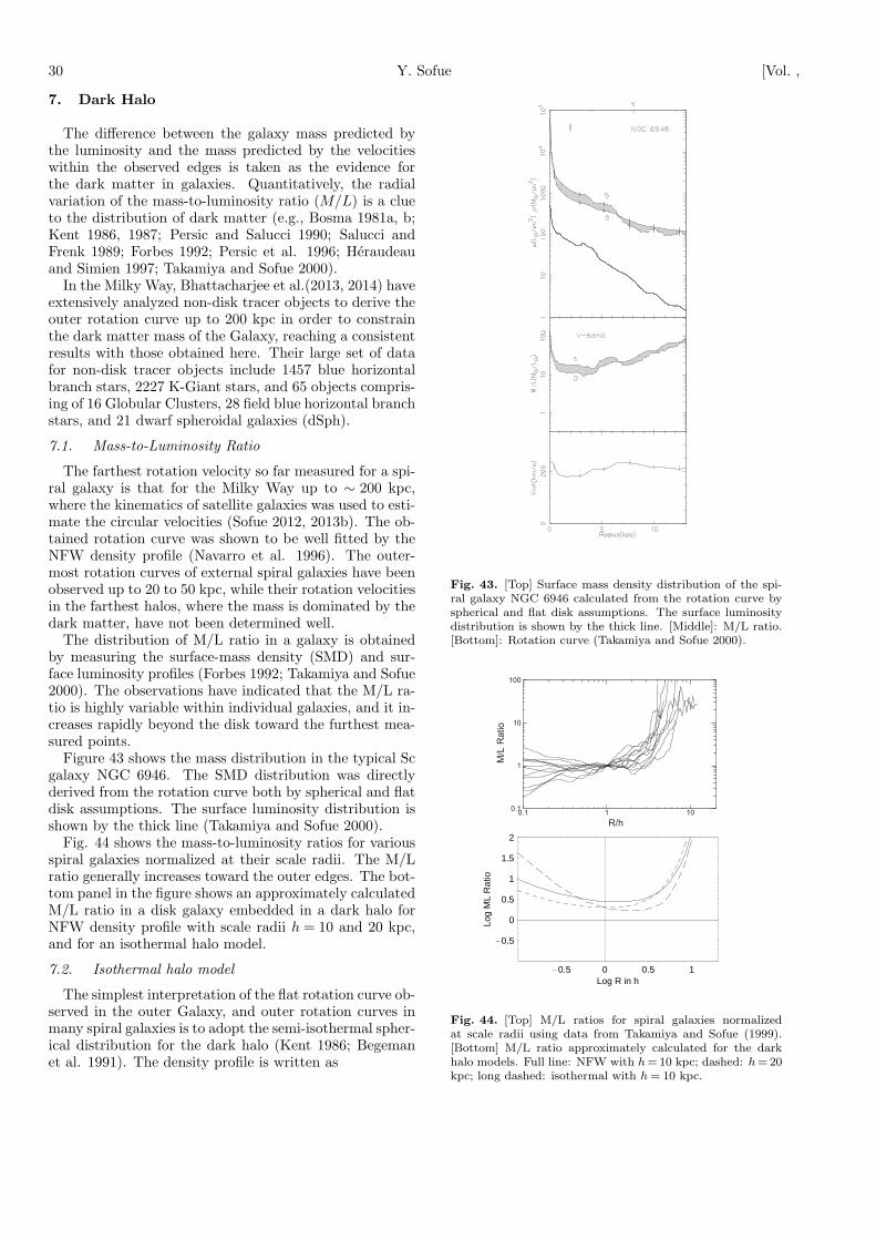
30 Y. Sofue [Vol. ,

7. Dark Halo

The difference between the galaxy mass predicted bythe luminosity and the mass predicted by the velocitieswithin the observed edges is taken as the evidence forthe dark matter in galaxies. Quantitatively, the radialvariation of the mass-to-luminosity ratio (M/L) is a clueto the distribution of dark matter (e.g., Bosma 1981a, b;Kent 1986, 1987; Persic and Salucci 1990; Salucci andFrenk 1989; Forbes 1992; Persic et al. 1996; Heraudeauand Simien 1997; Takamiya and Sofue 2000).

In the Milky Way, Bhattacharjee et al.(2013, 2014) haveextensively analyzed non-disk tracer objects to derive theouter rotation curve up to 200 kpc in order to constrainthe dark matter mass of the Galaxy, reaching a consistentresults with those obtained here. Their large set of datafor non-disk tracer objects include 1457 blue horizontalbranch stars, 2227 K-Giant stars, and 65 objects compris-ing of 16 Globular Clusters, 28 field blue horizontal branchstars, and 21 dwarf spheroidal galaxies (dSph).

7.1. Mass-to-Luminosity Ratio

The farthest rotation velocity so far measured for a spi-ral galaxy is that for the Milky Way up to ∼ 200 kpc,where the kinematics of satellite galaxies was used to esti-mate the circular velocities (Sofue 2012, 2013b). The ob-tained rotation curve was shown to be well fitted by theNFW density profile (Navarro et al. 1996). The outer-most rotation curves of external spiral galaxies have beenobserved up to 20 to 50 kpc, while their rotation velocitiesin the farthest halos, where the mass is dominated by thedark matter, have not been determined well.

The distribution of M/L ratio in a galaxy is obtainedby measuring the surface-mass density (SMD) and sur-face luminosity profiles (Forbes 1992; Takamiya and Sofue2000). The observations have indicated that the M/L ra-tio is highly variable within individual galaxies, and it in-creases rapidly beyond the disk toward the furthest mea-sured points.

Figure 43 shows the mass distribution in the typical Scgalaxy NGC 6946. The SMD distribution was directlyderived from the rotation curve both by spherical and flatdisk assumptions. The surface luminosity distribution isshown by the thick line (Takamiya and Sofue 2000).

Fig. 44 shows the mass-to-luminosity ratios for variousspiral galaxies normalized at their scale radii. The M/Lratio generally increases toward the outer edges. The bot-tom panel in the figure shows an approximately calculatedM/L ratio in a disk galaxy embedded in a dark halo forNFW density profile with scale radii h = 10 and 20 kpc,and for an isothermal halo model.

7.2. Isothermal halo model

The simplest interpretation of the flat rotation curve ob-served in the outer Galaxy, and outer rotation curves inmany spiral galaxies is to adopt the semi-isothermal spher-ical distribution for the dark halo (Kent 1986; Begemanet al. 1991). The density profile is written as

F . 4.ÈContinued

Fig. 43. [Top] Surface mass density distribution of the spi-ral galaxy NGC 6946 calculated from the rotation curve byspherical and flat disk assumptions. The surface luminositydistribution is shown by the thick line. [Middle]: M/L ratio.[Bottom]: Rotation curve (Takamiya and Sofue 2000).

R/h

M/LRatio

0.1 1 100.1

1

10

100

-0.5 0 0.5 1Log R in h

-0.5

0

0.5

1

1.5

2

Log

ML

Rat

io

Fig. 44. [Top] M/L ratios for spiral galaxies normalizedat scale radii using data from Takamiya and Sofue (1999).[Bottom] M/L ratio approximately calculated for the darkhalo models. Full line: NFW with h = 10 kpc; dashed: h = 20kpc; long dashed: isothermal with h = 10 kpc.

No. ] Review: Rotation and Mass of Galaxies 31

ρiso(R) =ρ0iso

1+ (R/h)2, (75)

where ρhc and h = Rh are constants giving the centralmass density and scale radius of the halo, respectively.This profile gives finite mass density at the center, butyields a flat rotation curve at large radius. The circularvelocity is given by

Vh(R) = V∞

√1−

(h

R

)tan−1

(R

h

), (76)

where V∞ is a constant giving the flat rotation velocity atinfinity. The constants are related to each other as

V∞ =√

4πGρ0isoh

2, (77)

or the central density is written as

ρ0iso = 0.740

(V∞

200km s−1

)(h

1kpc

)−2

M⊙pc−3. (78)

The enclosed mass within radius R is given by

M(R) = 4π

∫ R

0

ρi(r)r2dr (79)

with i = iso (NFW or Bur for the other two models asdiscussed below).

At small radius, R≪h, the density becomes nearly con-stant equal to ρ0

iso and the enclosed mass increases steeplyas M(R) ∝ R3. At large radius of R ≫ h the densitydecreases as ρiso ∝ R−2 and the enclosed mass tends toincrease linearly with radius as M(R) ∝ R.

7.3. NFW Profiles

Based on numerical simulations of the formation ofgalaxies in the cold-dark matter scenario in the expand-ing universe, several model profiles have been found tofit the calculated results. The most well known model isthe NFW model proposed by Navarro, Frenk and White(1996), and Burkert (1995) has modified this model. TheNFW and Burkert density profiles are written, respec-tively, as

ρNFW(R) =ρ0NFW

(R/h)/[1+ (R/h)2], (80)

and

ρBur(R) =ρ0Bur

[1+ (R/h)][1+ (R/h)2)]. (81)

The circular rotation velocity is calculated by

Vh(R) =

√GMh(R)

R, (82)

where Mh is the enclosed mass within h as calculated byequation (79).

At small radius with R ≪ h, the NFW density profilebehaves as ρNFW ∝ 1/R, yielding an infinitely increasingdensity toward the center, and the enclosed mass behavesas M(R) ∝ R2. On the other hand, the Burkert profiletends to constant density ρ0

Bur, yielding steeply increasing

(a)5 10 15 20 25 30

R kpc

50

100

150

200

250

300

Vkm

s

(b)5 10 15 20 25 30

R kpc

6

7

8

9

10

11

12

Log

Rho

Msu

nc.

kpc

(c)0 0.5 1 1.5 2 2.5 3

Log R kpc

10

10.5

11

11.5

12

12.5

13

Log

Mas

sM

sun

Fig. 45. (a) Schematic rotation curve composed of bulge,disk and dark halo components represented by isothermal,Burkert (1995) and NKF models (full lines from top to bottomat R = 30 kpc) - compared with the disk and bulge (dashedlines), and corresponding rotation curves.(b) Corresponding volume density.(c) Corresponding enclosed mass within radius r.

enclosed mass as M(R) ∝ R3, similarly to the isothermalprofile. At large radius with R ≫ h, both the NFW andBurkert profiles have densities ρNFW, Bur ∝R−3, and theyyield milder logarithmic increase of mass as M(R)∝ ln R(Fig. 45 )

Figure 45 shows density distributions for the three dif-ferent models of the dark halo as well those for the diskand bulge with scale radius h = 10 kpc. The figure alsoshows the masses enclosed within a sphere of radius R.In these figures, the total masses of the disk and halo aretaken to be the same at R = 15 kpc, so that the rota-tion velocity is nearly flat at R = 10 to 20 kpc and fit theobservations.

8. Plummer and Miyamoto-Nagai Potential

Although the deconvolution using the deVaucouleursand exponential disk well represents theobservations, the mass models are not necessarily self-consistent in the sense that the model mass profilesare the solutions of the Poisson equation. One of theconvenient methods to represent a galaxy’s mass distri-

32 Y. Sofue [Vol. ,

-20 -10 0 10 20R kpc

-10

-5

0

5

10

zkp

c

Bulge+Disk Rho

-20 -10 0 10 20R kpc

-10

-5

0

5

10

zkp

c

Cross section of Galaxy Bluge+Disk+Halo Rho

Fig. 46. Meridional cross section of volume-density in theGalaxy corresponding to figure 45 for the bulge and disk (top)and including dark halo. Contours are drawn every 0.2 dexof logarithm of density.

-20 -10 0 10 20R kpc

-10

-5

0

5

10

zkp

c

Bulge+Disk Sigma

-20 -10 0 10 20R kpc

-10

-5

0

5

10

zkp

c

Edge-on Galaxy Bulge+Disk+Halo Sigma

Fig. 47. Edge-on integrated view of surface mass densitiesfor figure 46. Contours are drawn every 0.2 dex of logarithmof surface density.

bution by a self-consistent dynamical solution is to usesuperposition of multiple Plummer-type potentials.

The mass distribution ρ(R,z) and the gravitational po-tential Φ(R,z) are related by the Poisson’s equation:

∆Φ = 4πρ(R,z), (83)

Let us recall that the potential for a point mass is givenby

Φ =−GM

r=

−GM√R2 + z2

, (84)

with r =√

R2 + z2 being the distance from the center. Anextended spherical mass is often described by a Plummer’slaw:

Φ =−GM√r2 + b2

=−GM√

R2 + z2 + b2. (85)

Here, b is a constant representing the scale radius of thesphere.

The most convenient Plummer-type formula, which de-scribes the potential and realistic mass distribution inthe Galaxy has, been obtained by Miyamoto and Nagai(1975). The potential is a modified one from equation (85)for an axisymmetric spheroid. A galaxy is representedby superposition of several mass components in the samefunctional form as

Φ =n∑

i=1

Φi =n∑

i=1

−GMi√R2 +(ai +

√z2 + b2

i )2, (86)

where, ai and bi are constants representing the scale radiusand scale height of the i-th spheroidal component. Therotation velocity in the galactic plane at z = 0 is given by

Vrot(R) =

√ n∑i=1

R∂Φi

∂R(87)

= R

√ n∑i=1

GMi

[R2 +(ai + bi)2]3/2.

The mass distribution is calculated from the Poisson’sequation 83:

ρ(R,z) =14π

n∑i=1

Mi×

aiR2 + [ai +3(z2 + b2

i )1/2][ai +(z2 + b2

i )1/2]2

R2 + [ai + (z2 + b2i )1/2]25/2(z2 + b2

i )3/2. (88)

Figure 48 shows the meridional distribution of volumemass-density calculated for a model Galaxy composed oftwo components of a bulge and disk with the param-eters as given in table 5 (Miyamoto and Nagai 1975).This model approximately reproduces the rotation curveand the Oort’s (1965) value of the local mass densityof 0.15M⊙pc−3 at R = 10 kpc. Note that the darkhalo was not taken into account, but instead the mass(2.5× 1011M⊙) and scale radius (7.5 kpc) were taken tobe larger than the present-day values of ∼ 1011M⊙ and∼ 3.5 kpc, in order to mimic the flat part of the rota-tion curve. Today, as discussed in the next section, theouter flat rotation is well understood as due to the darkhalo. Nevertheless, the MN potential is often used, for itsanalytical form, to represent a galaxy by modifying theparameters and adding the halo and central components.

Component Mi (M⊙) ai (kpc) bi (kpc)Bulge 2.05× 1010 0.0 0.495Disk 2.547× 1011 7.258 0.520

Table 5. Parameters determining the Miyamoto-NagaiPotential of the Galaxy.

9. Dynamical Parameters of the Bulge, Disk, andDark Halo in the Milky Way

In order to fit the observed rotation curve by models,we assume the following components:

No. ] Review: Rotation and Mass of Galaxies 33

-20 -10 0 10 20R kpc

-10

-5

0

5

10

zkp

c

Bulge

-20 -10 0 10 20R kpc

-10

-5

0

5

10

zkp

c

Disk

-20 -10 0 10 20R kpc

-10

-5

0

5

10

zkp

c

The Galaxy

-20 -15 -10 -5 0 50

0.20.40.60.8

1Log Rho in Msun per cub.pc

-20 -10 0 10 20R kpc

-200

-100

0

100

200

300

Vro

tkm

per

s

Rotation Curve

Fig. 48. Meridional distributions of the volume density inthe bulge, disk and their superposition to represent theGalaxy calculated for the Miyamoto-Nagai potential (1975)with parameters in table 5. Contours and grey scales arelogarithmic. The corresponding rotation curve is shown atbottom.

• The central black hole with mass MBH =4×106M⊙.• An innermost spheroidal component with the

exponential-sphere density profile, or a central mas-sive core.

• A spheroidal bulge with the exponential-sphere den-sity profile.

• An exponential flat disk.• A dark halo with NFW profile.

The approximate parameters for the disk and dark haloare adopted from the current study such as by Sofue(2012), and were adjusted here in order to better fit thedata. The inner two spheroidal components were fittedto the data by trial and error by changing the parametervalues, and the best-fit parameters are listed in table 9.Figure 39 shows the calculated rotation curve for theseparameters. The result satisfactorily represents the entirerotation curve from the central black hole to the outerdark halo.

We find that the fitting is fairly good in the GalacticCenter, and the inner two peaks of rotation curve at

r ∼ 0.01 kpc and ∼ 0.5 kpc are well reproduced by thetwo exponential spheroids. The figure also demonstratesthat the exponential bulge model is better than the deVaucouleursmodel.

Table 9 lists the fitting parameters for individual masscomponents. Since the used data were compiled from dif-ferent observations, their errors are not uniform, and onlyeye-estimated values are given, which were evaluated aftertrial and error of fitting to the observed points.

9.1. Local dynamical values

The local values of the surface mass and volume den-sities in the solar vicinity calculated for these parametersare also shown in table 9. The volume density of thedisk has been calculated by ρd = Σd/(2z0) with z0 beingthe scale height at R = R0, when the disk scale profile isapproximated by ρd(R0, z) = ρd0(R0)sech(z/z0). For thelocal galactic disk, two values are adopted: z0 = 144± 10pc for late type stars based on the Hipparcos star cata-logue (Kong and Zhu 2008) and 247 pc from Kent et al.(1991).

The local volume density by the bulge is four orders ofmagnitudes smaller than the disk component, and the halodensity is two orders of magnitudes smaller. However, thesurface mass densities as projected on the Galactic planeare not negligible. The bulge contributes to 1.6% of thedisk value, or the stars in the direction of the galacticpole would include about 2% bulge stars, given the deVaucouleurs density profile. The surface mass density ofthe dark halo integrated at heights of −10 < z < 10 kpcexceeds the disk value by several times.

9.2. Local dark matter density

The local density of the dark matter is the essentialquantity in direct experimental detection in relation tothe origin and physics of the dark matter. The NFWprofile was found to fit the grand rotation curve quitewell (Sofue 2012). The declining part in the outermostrotation velocity predicted by the NFW profile was clearlydetected, showing the good fit to the outermost grandrotation curve at R ∼ 40− 400 kpc covering the Galaxy’sgravitational boundary.

According to the best fit parameters for the NFWmodel, the local value of the dark matter density in theSolar neighborhood is calculated to be ρ⊙0 = 0.235±0.030GeV cm−3. This value may be compared with the valuesobtained by the other authors as listed in table 7

10. Direct Mass Determination

In the above methods, several mass components are as-sumed a priori, each of which had representative func-tional form, and therefore, the results depend on the as-sumed profiles. In order to avoid this dependence on theadopted functions, a direct method to obtain the massdistribution without assuming the functional form can beapplied, where the mass distribution is calculated directlyusing the observed rotation velocity data. Since the rota-tion curve is restricted to give force in the galactic plane,

34 Y. Sofue [Vol. ,

Table 6. Parameters for the mass components of the Galaxy (Sofue 2013b) †

Mass component Scale radius / Mass / DensityBlack hole Mbh = 3.6× 106M‡

⊙Bulge 1 (massive core) ab = 3.5± 0.4 pc

Mb = 0.4± 0.1× 108M⊙Bulge 2 (main bulge)∗ ab = 120± 3 pc

Mb = 0.92± 0.02× 1010M⊙Disk ad = 4.9± 0.4 kpc

Md = 0.9± 0.1× 1011M⊙Dark halo h = 10± 0.5 kpc

ρ0 = 2.9± 0.3× 10−2M⊙pc−3

MR<200kpc = 0.7± 0.1× 1012M⊙MR<385kpc = 0.9± 0.2× 1012M⊙

Local DM density at R = 8 kpc ρ8 = 0.011± 0.001M⊙pc−3

= 0.40± 0.04GeV cm−3

† The adopted galactic constants are (R0,V0) =(8 kpc, 238 km s−1) (Honma et al 2012).‡ Genzel et al. (2000; 2010∗ Mb is the surface mass enclosed in a cylinder of radius ab, but not a spherical mass.

Table 7. Local dark matter density near the Sun in the Galaxy from the literature.

Author Dark matter density (GeV cm−3)Weber and de Boer (2010) 0.2 - 0.4Salucci et al. (2012) 0.43± 0.10Bovy and Tremaine (2012) 0.3± 0.1Piffl et al. (2014) 0.58Sofue (2013b) for V0 = 200 km s−1 0.24± 0.03—– for V0 = 238 km s−1 0.40± 0.04Pato et al (2015a,b) V0 = 230 km s−1 0.42± 0.25

the method cannot give the three dimensional informa-tion. Hence, a ’true’ mass profile in a real disk galaxy isassumed to lie between two extreme profiles, which areeither spherical or axisymmetric flat-disk.

10.1. Spherical Mass Distribution from Rotation Curve

The mass M(R) of a spherical body inside radius R isgiven by

M(R) =RV (R)2

G, (89)

where V (R) is the rotation velocity at r. Then the SMDΣS(R) at R is calculated by,

ΣS(R) = 2

∞∫0

ρ(r)dz =12π

∞∫R

1r√

r2 −R2

dM(r)dr

dr. (90)

The volume mass density ρ(R) is given by

ρ(R) =1

4πr2

dM(r)dr

. (91)

For a given rotation curve V (R), equation (90) can becomputed numerically. In a galaxy, this gives a good ap-proximation for the central region where the spheroidalcomponent dominates. On the other hand, the equationgives underestimated mass density near the outer edge at

R ∼ Rmax because of the edge effect due to the finite ra-dius of data points. The edge effect is negligible in theusual disk regions.

10.2. Flat-Disk Mass Distribution

The surface mass density (SMD) for a thin disk, ΣD(R),can be obtained by solving the Poisson’s equation on theassumption that the mass is distributed in a flat disk withnegligible thickness. It is given by

ΣD(R) =1

π2G× 1

R

R∫0

(dV 2

dr

)x

K( x

R

)dx +

∞∫R

(dV 2

dr

)x

K

(R

x

)dx

x

,(92)

where K is the complete elliptic integral and becomes verylarge when x ≃ R (Freeman 1970; Binney and Tremaine1987). For the calculation, it must be taken into accountthat equation (92) is subject to the boundary condition,V (0) = V (∞) = 0. Also it is assumed that V (0) = 0 at thecenter. Since a central black hole of a mass on the orderof 106 − 107M⊙ dominates the RC only within a few pc,it does not influence the galactic scale SMD profile.

When calculating the first term on the right hand sideof equation (92) for the central region, it happens thatthere exist only a few data points, where the reliability

No. ] Review: Rotation and Mass of Galaxies 35

of the calculated V (R) is lower than the outer region. Inaddition, the upper limit of the integration of the secondterm is Rmax instead of infinity. Since the rotation curvesare nearly flat or declining outward from R = Rmax, thesecond term becomes negative. Thus, the values are usu-ally slightly overestimated for ΣD(R) at R ≃ Rmax.

10.3. The Milky Way

Figure 49 shows the obtained direct SMD distributionin the Galaxy. There is remarkable similarity betweenthis result and the total SMD obtained by deconvolutionof the rotation curve into the bulge, disk and halo com-ponent. The mass is strongly concentrated toward thenucleus, and the bulge component dominates in the cen-tral region. The calculated SMD reaches a value as highas ∼ 105M⊙ pc2 at radius of a few tens pc. Higher den-sity concentration has been observed from high-resolutioninfrared photometry and spectroscopy, indicating SMD ashigh as ∼ 106M⊙ pc3 within a few pc (Genzel et al. 1996).These values may be compared with the central value ofthe bulge’s SMD as fitted by the de Vaucouleurs profile,Σbc = 6.8× 106M⊙ pc2, from equation 62.

The galactic disk appears as the straight-line part atR∼ 3 to 8 kpc on this semi-logarithmic plot (R vs log Σ),indicating the exponential character. Even in these radii,as well as in the solar vicinity at R∼ 8 kpc, the dynamicalsurface mass (not volume density) is dominated by thedark matter, because the SMD is the projection of hugeextent of the dark halo. There is slight difference betweenSMDs from the deconvolution method and direct method:for example at R ∼ 8 kpc, the SMD is ∼ 300M⊙ pc−2 inFig.50, whereas it is ∼ 200−250M⊙ pc−2 in Fig.49 . Thisdiscrepancy is due to the difference caused by the limitedareas of integration from the finite data for the infinitelyextended dark halo as well as due to difference in theadopted methods.

The outer disk, as indicated by the flat-disk model (fullline in Fig. 49), is followed by an outskirt with a moreslowly declining density profile, gradually detaching fromthe straight line part of the disk. This outskirt indicatesthe dark halo, which extends to much larger radii, as isdiscussed in the next section.

In figure 49, we also show the radial distribution of in-terstellar gas density, as calculated by azimuthally aver-aging the gas density distribution in figure 14. The gasdensity is much smaller than the dynamical mass densityby an order of magnitude. In fact, the interstellar gasdensity at R ∼ 8 kpc is ∼ 5.0M⊙pc−2, which shares onlyseveral percents of disk mass density of ∼ 87.5M⊙pc−2.

10.4. Spiral Galaxies

The mass distributions in spiral galaxies can be alsodirectly computed from observed rotation curves in thesame way as for the Milky Way. Figure 50 shows theSMD distributions of Sb galaxies obtained for the rotationcurves in Fig. 27 using equation 92. The central regionsare enlarged in the bottom panel, where equation (90) isadopted for a spherical model, which better represents theinner spheroidal components.

R (kpc)

SMD(Msun/sq.pc)

H2 HI

Gas

SMD

0 5 10 15 2010-1

100

101

102

103

104

105

Fig. 49. Radial distribution of the surface-mass density(SMD) in the Galaxy directly calculated from the rotationcurve for thin disk (thick line). The thin line is the result forspherical assumption which better represents the innermostbulge component, where the outer truncation is due to edgeeffect. The lower lines show SMD of interstellar gas made byannulus-averaging the face-on projected distribution in Fig.14 (Nakanishi and Sofue 2003, 2006). HI and H2 gas SMDsare also shown separately by dotted lines.

The calculated SMD profiles for the Sb galaxies aresimilar to that of the Milky Way. It is also known thatthe profiles for Sa to Sc galaxies are very similar to eachother, except for the absolute values (Takamiya and Sofue2000). It is stressed that the dynamical structure repre-sented by the density profile is very similar to each otheramong spiral galaxies. The SMD profiles have a univer-sal characteristics as shown in these figures: high centralconcentration, exponential disk (straight line on the semi-logarithmic plot), and outskirt due to the dark halo.

10.5. Enclosed mass

It is worthwhile to examine if the present result is con-sistent with the previous works by other authors. For thispurpose, we compare our result with the measurementsand compilation of enclosed mass data by Genzel et al.(1994), which have been obtained using various kinds ofobjects such as giant stars, He I stars, HI and CO gases,circum-nuclear disk, and mini spirals (See the literaturetherein for details).

Figure 53 shows the enclosed mass as a function of ra-dius calculated by the presently fitted model. In the figurewe overlaid the results by Genzel et al. (1994), where theirdata have been converted to the case of R0 = 8.0 kpc from8.5 kpc adopted in their paper, multiplying the radiusscale by 8.0/8.5=0.94. The mass scale was also multi-plied by the same amount, as the mass is proportional to∝ rv2, while radial velocities v toward the Galactic Centerare hardly affected by the galacto-centric distance.

The enclosed mass for the black hole is trivially con-stant. The inner and main bulges have constant densitynear the center, which yields enclosed mass approximatelyproportional to ∝ r3 after volume integration. The diskmodel has constant surface density near the center, yield-

36 Y. Sofue [Vol. ,

Fig. 50. Surface-mass density distributions in Sb galaxies us-ing flat-disk. Bottom is the same but for the central regionsusing spherical model (Takamiya and Sofue 2000).

R (kpc)

SMD(Msun/sqpc)

0.001 0.01 0.1 1 10102

103

104

105

Fig. 51. Logarithmic SMD distributions of galaxies (fulllines) compared with that for the Galaxy (dash with filledcircles) directly calculated with observed rotation curves forflat-disk assumption.

ing enclosed mass ∝ r2 for surface integration. However,it would be much less because of the finite thickness forthe real galactic disk. The NFW model predicts a highdensity cusp near the center as ∝ r−1, yielding enclosedmass proportional to ∝ r2. However, the dark matter den-sity may not be taken so serious because of the unknownaccuracy of the model in the vicinity of the nucleus.

The figure shows that the present result is in good agree-ment with the previous observations. We stress that thewavy variation in our profile due to the two-componentbulge structure is also observed in the stellar kinematicsresults.

R (kpc)

SMD(Msun/sqpc)

Inner Bulge(Core)

Bulge

Disk

Dark Halo

10-3

10-2

10-1

100

101

102

103

10-1

100

101

102

103

104

105

106

R (kpc)

SMD(Msun/sqpc)

0 5 10 1510

1

102

103

104

105

106

Fig. 52. Left: Surface-mass density profiles. Solid line showsSMD calculated by using the model rotation curve in sphericalassumption. Thin dashed lines show individual components.Thick dashed line is SMD in flat-disk assumption. Grey dotsand open circles show SMD calculated by using the observedrotation curve in spherical and flat-disk assumptions, respec-tively. Right: Same, but direct mass alone in semi-logarithmicpresentation with the exponential disk by dashed line.

Fig. 53. Comparison of enclosed mass calculated for thepresent rotation curve with the current results compiled byGenzel et al. (1994: see the literature therein for the plotteddata). Horizontal line indicates the central black hole, thinlines show the inner bulge, main bulge and disk. The dashedline shows dark matter cusp.

No. ] Review: Rotation and Mass of Galaxies 37

10.6. Effect of non-circular motions on mass determi-nation

The rotation curve analysis cannot treat the non-axisymmetric part of the Galaxy (11) to (27) as listed intable 1. It is true that the galactic disk is superposed bynon-circular streaming motions such as due to bars, armsand expanding rings. However, it is not easy to derivenon-axisymmetric mass distribution from the existing ob-servations. Simulations based on given parameters of barpotential can produce LV diagrams, and may be comparedwith the observations (Binney et al. 1991; Jenkins andBinney 1994; Athnasoula 1992; Burton and Liszt 1993).The present analysis would be a practical way to approachthe dynamical mass structure of the central Galaxy.

We comment on the accuracy of the present analysis.The non-circular motions observed in the LV diagramsare as large as ∼ ±20− 30% of the circular velocity. Inthe present analysis, these motions yield systematic errorsof ∼ 40 − 60% of mass estimation, and the accuracy ofobtained mass is about ±60%, or within a factor of ∼ 1.6.

The agreement of the present analysis with those fromthe stellar dynamics by Genzel et al. (1994) as shown infigure 53 may indicate that the bar’s effect will not be sosignificant in the central several tens of parsecs. Stellarbar dynamics and stability analysis in the close vicinity ofthe massive black hole would be a subject for the future.It is an interesting subject to examine if such a stronggravity by the central mass structures may allow for along-lived bar.

11. Size and Mass Relations among the MassComponents

Decomposition of rotation curves is a powerful tool tostudy the relations among the scale radii and masses ofthe bulge and disk with those of the dark halo, whichprovides with important information about the structureformation in the universe (Reyes et al. 2012; Miller et al.2014; Behroozi et al. 2013). Sofue (2015b) has obtainedthe relations using tens of nearby spiral galaxies by com-piling rotation curves of more than one hundred galaxiesas shown in figure 26. The decomposition was appliedby adopting the de Vaucouleurs, exponential and NFWdensity profiles for the bulge, disk and dark halo, respec-tively. The best-fitting values were obtained by applyingthe least χ2 method for Mb, ab, Md, ad, ρ0 and h. Thecritical dark halo radius, R200, critical mass, M200, as wellas the mass, Mh, enclosed within the scale radius h werealso calculated, which are defined by

M200 = 200ρc4π

3R3

200, (93)

and

ρc = 3H20/8πG, (94)

with H0 = 72 km s−1Mpc−1 being the Hubble constant.Figure 54 shows examples of rotation curves and fitting

result for NGC 891. The figure also show the variationof χ2 values plotted against the parameters. Applying a

Fig. 54. Rotation curve and χ2 fitting result for NGC 891(top), distribution of χ2/N around the best fit scale radii(middle) and masses (bottom) of the three components.

selection criterion, the fitting was obtained for 43 galaxiesamong the compiled samples in figure 26, and the meanvalues of the results are shown in table 8.

Figure 55 shows plots of ab, ad, and h against the crit-ical radius R200. It is shown that the bulge, disk and haloscale radii are positively correlated with R200. Note, how-ever, that the tight correlation between h and R200 par-tially includes a trivial internal relation due to the def-inition of the two parameters connected by ρ0 throughequation (93).

The figure also shows Mb+d plotted against M200, whichmay be compared with the relation of stellar masses ofgalaxies against dark halo masses as obtained by cosmo-logical simulation of star formation and hierarchical struc-ture formation by Behroozi et al. (2013). The grey dashedline shows the result of simulation at z = 0.1.

Figure 56 shows the bulge+disk mass, Mb+d, plottedagainst total mass, M200+b+d = M200 +Mb+d. In the fig-ure we also plot photometric luminous mass and Virialmass obtained for dwarf galaxies by Millar et al. (2014).Also compared is a cosmological simulation by Behrooziet al. (2013). The simulation is in agreement in its shapewith the plots for spiral galaxies and dwarfs. The shapeof simulated relation is consistent with the present dy-namical observations, while the absolute values of Mb+d

are greater than the simulated values by a factor of three.Solving the discrepancy may refine the cosmological mod-els and will be a subject for the future.

The positive correlations between the size and massboth for bulges and disks, particularly the disk’s size-mass relation, are the dynamical representation of the

38 Y. Sofue [Vol. ,

Table 8. Mean parameters for selected galaxies (Sofue 2015b).

Number of galaxies . . . 43Bulge size . . . . . . . . . . . . ab (kpc) 1.5± 0.2— mass . . . . . . . . . . . . . . . Mb(1010M⊙) 2.3± 0.4Disk size . . . . . . . . . . . . . . ad(kpc) 3.3± 0.3— mass . . . . . . . . . . . . . . . Md(1010M⊙) 5.7± 1.1Dark Halo scale size . . h (kpc) 21.6± 3.9— mass within h . . . . . . Mh(1010M⊙) 22.3± 7.3—critical radius . . . . . . . R200 (kpc) 193.7± 10.8— critical mass . . . . . . . M200(1010M⊙) 127.6± 32.0Bulge+Disk mass . . . . . . Mb+d(1010M⊙) 7.9± 1.2Bulge+Disk+Halo mass M200+b+d(1010M⊙) 135.6± 32.0B+D/Halo mass ratio . Mb+d/M200 0.062± 0.018B+D/Total mass ratio . Mb+d/M200+b+d 0.059± 0.016

(a)R200 (kpc)

Ab,Ad,h(kpc)

10070 80 90 200 300 400 500

0.1

1

10

100

(b)R200 (kpc)

Mb,Md,Mh,M200(Msun)

10070 80 90 200 300 400 500

108

109

1010

1011

1012

1013

(c)M200 (Msun)

Mb,Md,Mbd(Msun)

1011 1012 1013108

109

1010

1011

1012

Fig. 55. (a) Size-Size relations for dark halo critical radius for (R200,ab) (triangles); (R200,ad) (open circles); and (R200,h) (blackdots) (Sofue 2015b).(b) Size-Mass relations for (R200,Mb) (triangles); (R200,Md) (rectangles); (R200,Mh) (black dots); (R200,M200) (grey small dots)showing the trivial relation by definition of the critical mass.(c) Mass-Mass relations for (M200,Mb) (triangles); (M200,Md) (rectangles); and (M200,Mb+d) (black dots). Dashed grey line showsthe cosmological simulation + photometry (Behroozi et al. 2013).

luminosity-size relation established by optical and infraredphotometry (de Jong et al. 1999; Graham and Worley2008; Simard et al. 2011). It should be stressed that thesame size-mass relation applies to the dark halo.

The plotted size-mass relations can be represented bythe following equations, which were obtained by the least-squares fitting in the log-log plane by linear functions.Measuring the mass and scale radii in M⊙ and kpc, re-spectively, we have for the disk and dark halo

log10Md = (9.89± 0.23) + (1.38± 0.41) log10ad, (95)

log10Mh = (9.26± 0.52) + (1.45± 0.43) log10h, (96)

while the relation for the bulge is too diverged to be fittedby a line. The size-mass relation for the disk is consistentwith the luminosity-size relation obtained by Simard etal. (2011). Both the size to mass relations for the diskand dark halo can be represented by a single relation

log10Mi = (10.18± 0.24)+ (1.38± 0.21)log10ai, (97)

where Mi = Mb+d or M200 in 1010M⊙ and ai = ad or h inkpc. This simple equation leads to a relation between thebulge+disk mass to halo mass ratio, which approximatelyrepresent the baryonic fraction, expressed by the ratio ofthe scale radii of disk to halo as

Mb+d/M200 ≃ (ad/h)1.38. (98)

For the mean values of < ad >= 3.3 kpc and < h >= 21.6kpc, we obtain Mb+d/M200 ∼ 0.07.

No. ] Review: Rotation and Mass of Galaxies 39

Fig. 56. Mb+d-M200+b+d relation compared with the stellarmass-total mass relation for dwarf galaxies (triangle: Milleret al. 2014) and simulation + photometry (grey dashed line:Behroozi et al. 2013). Black dots are the selected galaxieswith reasonable fitting results, while small grey dots (includ-ing black dots) show non-weighted results from automatic de-composition of all rotation curves.

5. CONCLUDING REMARKS

1. summary

Rotation curve is the most fundamental tool to discussthe dynamics and mass distribution in the Galaxy and indisk galaxies, and there are various methods to derive ro-tation curves. In this review, various methods to deriverotation curves of the Galaxy and spiral galaxies were de-scribed, and explanations were given of the methods tocalculate the mass distribution using the rotation curve.Observed rotation curves for the Milky Way as well as fornearby spiral galaxies were presented, and were used toderive the mass distributions.

The mass distribution is determined both by dynami-cal and photometric methods. The dynamical method wasdescribed in detail in this review. Compared to the pho-tometric methods, which assume the mass-to-luminosityratio, the dynamical method is more direct to measure themass including the dark matter and black holes.

The dynamical method may be further categorized intotwo ways: one is the decomposition method, by which therotation curve is fitted by a calculated one as summationof several mass components. The dynamical parameters ofindividual components are determined during the fittingprocedure. This method is convenient to discuss sepa-rately the basic galactic structures, which are usually thecentral massive object, bulge, disk and dark halo. Each ofthese components may have its own evolutional and dy-namical properties. Inconvenience of this method is thatone has to assume a priori the functional forms for themass components, which may not necessarily be unique.Therefore, the results depend on the adopted model.

Another method is the direct method, in which the massdistribution is directly calculated from the data of rota-tion velocity. This method does not employ any galactic

models or functional forms, but straightly compute themass distribution. The results can be compared with sur-face photometry to obtain the distribution of the mass-to-luminosity ratio, dividing the surface-mass density by sur-face luminosity. The thus computed M/L ratio generallyincreases monotonically toward the edges of spiral galax-ies, giving a direct evidence for dark matter halo. Thedecomposition and direct methods are, of course, compli-mentary and the derived mass distributions are usuallyconsistent with each other.

It was shown that the rotation characteristics of spiralgalaxies are similar to each other, and so are the mass dis-tributions. The dynamical back bones are, thus, universalfrom Sa to Sc galaxies, and the structures are almost iden-tical among the galaxies in so far as the dynamical mass isconcerned. The Milky Way exhibits representatively theuniversal characteristics from the central black hole to thedark halo.

The dark halo of the Galaxy and M31 were shown tobe fitted by the NFW and Burkert profiles better thanthe isothermal or similar models postulating flat rotationto the ends. It was also shown that the dark halo ex-tends far out to the intracluster space almost a half wayto M31, where the dark matter properly possessed by theLocal Group dominates in order for the Local Group tobe gravitationally bound. Rotation curves of a large num-ber of galaxies were deconvolved into bulge, disk and darkhalo by the decomposition method. Statistics among thederived parameters showed positive correlation of the diskand bulge masses with the dark halo mass.

2. Achievements in the decades and the future

In our previous review (Sofue and Rubin 2001) variousadvances have been expected for the future rotation curvestudies thanks principally to instrumental developments.We summarize and evaluate the progress in the decades.

2.1. Extinction-free rotation kinematics in the central re-gions

This has been achieved extensively using CO line spec-troscopy and imaging, and will be achieved in an ulti-mate way using the ALMA (Atacama Large mm andsubmm Array) with higher spatial (0.01 arcsec) resolu-tion. Spectroscoy with eight- and ten-meter class opti-cal/infrared telescopes using infrared spectral lines suchas Br γ was anticipated, while the progress seems notfast, and no outstanding advances have been achieved.

2.2. VLBI astrometry

The VERA (VLBI Experiments for Radio Astrometry)observations have successfully achieved high-resolution as-trometric measurements of paralactic distances, positions,proper motions, and radial velocities for a number ofmaser sources in the Milky Way. The observations re-sulted in a number of papers in a series of special volume inPASJ. Many new aspects have been learnt in details of thethree-dimensional kinematics of the Galaxy, which includethe new values of (R0,V0) (distance to the Galactic Center,

40 Y. Sofue [Vol. ,

the Solar rotation velocity), non-circular motions relatedto the density waves and bars. SKA (Square-KilometerArray) will be a future, probably more powerful tool forthe trigonometric determination of the Galactic rotationcurve and dynamics even by simply extending the methodemployed with VERA.

2.3. High-redshift rotation curves

Thanks to the increase of aperture and sensitivity of thetelescopes, particularly using HST and 8-10 meter tele-scopes, galaxies have at cosmological distances becometargets for rotation curve observations. Although not fastas expected, there have been tens of galaxies at high red-shifts have been measured of rotation velocities. The dataare still not sensitive enough to be compared with thosefor the nearby galaxies at z =0. The rotation curve shapesseems to be similar already at z ∼ 3− 5, several billionsyears ago. Combined with cosmological simulations ofstructural formation and evolution, this field would beone of the most important aspects in the rotation curvestudy in the near future.

2.4. Method of analysis

Sophisticated methods of analysis of rotation curves in-volving 2D and 3D velocity fields were expected to beachieved to produce more accurate rotation curves forlarge samples of spirals. These will lead to more tightlyconstrained mass deconvolution, and distribution of darkand luminous matters. However, not much advances wereobtained in this field.

2.5. Bars and spiral arms

In this paper, we reviewed on rotation curves basedon the assumption that the galactic rotation is circularand axisymmetric. Hence, we did not touch upon such afundamental parameter as the pattern speed spiral armsand/or bars. However, observed kinematical data are themixture of pure rotation and various perturbations mainlyproduced by bars and spiral arms. The separation of barrelated quantities is still difficult even though the data getwider, deeper, and more accurate. The number of param-eters, and hence the number of freedom for the fitting, istoo large to reach a unique result. The problem is morecomplicated for the spiral arms, which have larger numberparameters than a bar.

2.6. Dark halos

Dark halos are one of the major topics in the fieldnot only of galaxy dynamics and kinematics but also ofthe structure formation and evolution in the expandinguniverse. As to the Milky Way and M31, it has beenshown that their rotation curves, and hence the dark mat-ter halos, seem to be merged at a half distance to eachother. Both galaxies showed declining rotation, not flatany more, in the outermost halos, which are well approxi-mated by the NFW model. However, direct measurementsof the dynamical mass of dark halos in external galaxiesare limited only to several tens of galaxies. Moreover,their outermost radii of measured rotation curves are too

small, mostly up to ∼ 20− 30 kpc. Wider view measure-ments up to ∼ 100 kpc for a more number of galaxies arecrucial for conclusive comparison with the cosmologicalscenarios of structure formation and evolution.

The physical property of the dark matter in view of el-ementary particle physics would be clarified when a di-rect detection and measurement in the laboratory wasachieved. A number of attempts to detect the dark mat-ter directly in the laboratory, when the dark matter den-sity in the solar neighborhood has been determined in therange around ∼ 0.2−0.4GeV cm −3. Also indirect detec-tion toward the Sun or the Galactic Center are proposedand partly performed. At this moment, there appears noreport of firm detection.

2.7. Supermassive black holes

Coevolution of the spheroidal component and centralsupermassive black hole may be a standard scenario in thestructural evolution of galaxies based on the observationalfacts that black hole mass is positively correlated withthe spheroidal mass in measured galaxies. This topic was,however, not reviewed in this paper, mainly because ofinsufficient sample galaxies with both the black hole massand detailed rotation curves. Such study would be aninteresting subject for the future.

2.8. Galactic activities

Many of the galaxies with well defined rotation curves asdiscussed in this review are known as galaxies possessingvarious activities such as starburst, outflow, jets, and/orAGN (active galactic nuclei). However, there has beenno clear correlation analysis among these activities andthe galactic mass distribution. It could be a subject fora more detailed comparison study with careful inspectionof the individual curves and mass structures, categorizingthe curves with and without the activities.

Correlation analysis of general star forming activity inthe disk with the rotation curves and mass structure wouldbe also a fundamental subject for galaxy evolution anddisk formation. In fact, a clear relation is readily knownby the relation that low surface brightness galaxies aregenerally more slowly rotating and therefore less massive.On the other hand, high velocity rotators are usually latetype as Sa to S0, and their star formation activity hasalready passed in the far past exhibiting high rate of starformation. This could be more directly confirmed by ob-serving high-redshift galaxies of their star formation rateand rotation curve simultaneously.

References

Aaronson M, Mould J. 1986. Ap. J. 303:1Amram P, Marcelin M, Balkowski C, Cayatte V, Sullivan III

WT, Le Coarer E. 1994. Astron. Astrophys. Supp. 103:5Battinelli, P., Demers, S., Rossi, C., and Gigoyan, K. S. 2013,

Astrophysics, 56, 68Begeman KG, Broeils AH, Sanders RH. 1991. MNRAS 249:523Begeman KG. 1989 AA 223:47Behroozi, P. S., Wechsler, R. H., & Conroy, C. 2013, ApJ, 770,

57

No. ] Review: Rotation and Mass of Galaxies 41

Bershady, M. A., Verheijen, M. A. W., Westfall, K. B., et al.2010, ApJ, 716, 234

Bershady, M. A., Verheijen, M. A. W., Swaters, R. A., et al.2010, ApJ, 716, 198

Bertola F, Cappellari M, Funes JG, Corsini EM, Pizzella A,Vega Bertran JC. 1998. Ap. J. Lett. 509:93

Bhattacharjee, P., Chaudhury, S., Kundu, S., and Majumdar,S. 2013, Phys. Rev. D, 87, 083525

Bhattacharjee, P., Chaudhury, S., and Kundu, S. 2014, ApJ,785, 63

Binney, J., and Dehnen, W. 1997, MNRAS, 287, L5Binney J, Gerhard OE, Stark AA, Bally J, Uchida KI 1991

MNRAS 252:210Binney J, Tremaine S. 1987, in Galactic Dynamics . Princeton

Univ. PressBlais-Ouellette, S., Amram, P., Carignan, C. 2001 AJ 121,

1952Blais-Ouellette, S., Amram, P., Carignan, C., and Swaters, R.

2004, A&A, 420, 147Blitz L. 1979. Ap. J. 227:152Blitz, L., Fich, M., Stark, AA 1982, ApJs, 49, 183Bobylev, V. V. 2013, Astronomy Letters, 39, 95Bobylev, V. V., & Bajkova, A. T. 2015, Astronomy Letters,

41, 473Bosma A. 1981a. AJ 86:1825Bosma A. 1981b. AJ 86:1791Bovy, J., & Tremaine, S. 2012, ApJ, 756, 89Broeils AH. 1992. Astron. Astrophys . 256:19Burkert, A., 1995, ApJ, 447, L25Burton, W. B. , Gordon, M. A. 1978 AA 63, 7.Burton, W. B. and Liszt H. S. 1993 AA 274, 765.Buta R, Purcell GB, Cobb ML, Crocker DA, Rautiainen P,

Salo H. 1999. Astron. J. 117:778Carignan C, Beaulieu S. 1989. Ap. J. 347:760Carignan C, Freeman KC. 1985. Ap. J. 294:494Carignan C, Puche D. 1990a. AJ 100:394Carignan C, Puche D. 1990b. AJ 100:641Carignan, C., Chemin, L., Huchtmeier, W. K., and Lockman,

F. J. 2006, ApJL, 641, L109Catinella, B., Giovanelli, R., and Haynes, M. P. 2006, ApJ,

640, 751Chemin, L., Carignan, C., and Foster, T. 2009, ApJ, 705, 1395

, A&A, 511, A89Ciotti L., 1991, AA, 249, 99.Clemens, D. P. 1985. ApJ 295:422Corradi RLM, Boulesteix J, Bosma A, Amram P, Capaccioli

M. 1991. Astron. Astrophys. 244:27Courteau, S. 1997. AJ 114:2402de Blok WJG, McGaugh SS, van der Hulst JM. 1996. MNRAS

283:18de Blok, W. J. G. 2005 ApJ 634 227de Blok, W. J. G., McGaugh, S. S., and Rubin, V. C. 2001,

AJ, 122, 2396de Blok, W. J. G., and Bosma, A. 2002, A&A, 385, 816de Blok, W. J. G., Walter, F., Brinks, E., et al. 2008, AJ, 136,

2648de Vaucoureurs, G. 1958, ApJ, 128, 465Dehnen, W., and Binney, J. 1998, MNRAS, 294, 429Demers, S., Battinelli, P. 2007 AA, 473, 143.Di Teodoro, E. M., & Fraternali, F. 2015, MNRAS, 451, 3021Epinat, B., Tasca, L., Amram, P., et al. 2012, A&A, 539, AA92Erb, D. K., Shapley, A. E., Steidel, C. C., et al. 2003, ApJ,

591, 101Erroz-Ferrer S., et al., 2012, MNRAS, 427, 2938

Feast, M., and Whitelock, P. 1997, MNRAS, 291, 683Ferrarese L, Ford HC. 1999. Ap. J. 515:583Fich, M., Blitz, L., Stark, A. A. 1989 ApJ 342, 272Fich, M,, Tremaine, S. 1991 ARAA, 29, 409Forbes, DA. 1992 AAS 92:583Freeman, K. C. 1970, ApJ, 160, 811Garrido, O., Marcelin, M., Amram, P., and Boulesteix, J. 2002,

A&A, 387, 821Garrido, O., Marcelin, M., and Amram, P. 2004, MNRAS, 349,

225Garrido, O., Marcelin, M., Amram, P., et al. 2005, MNRAS,

362, 127Gentile G., Salucci P., Klein U., Granato G. L., 2007, MNRAS,

375, 199Gentile G., et al., 2015, A&A, 576, A57Genzel, R., Hollenbach, D., and Townes, C. H. 1994, Reports

on Progress in Physics, 57, 417Genzel R, Eckart A, Ott T, Eisenhauer F. 1997. MNRAS

291:219Genzel R, Pichon C, Eckart A, Gerhard OE, Ott T. 2000

MNRAS 317:348Genzel, R., Pichon, C., Eckart, A., Gerhard, O. E., and Ott,

T. 2000, MNRAS, 317, 348Genzel, R., Thatte, N., Krabbe, A., Kroker, H., Tacconi-

Garman, L 1996 ApJ 472, 153Genzel, R., Burkert, A., Bouche, N., et al. 2008, ApJ, 687, 59Genzel, R., Eisenhauer, F., and Gillessen, S. 2010, Reviews of

Modern Physics, 82, 3121Genzel, R., Newman, S., Jones, T., et al. 2011, ApJ, 733, 101Ghez A, Morris M, Klein BL, Becklin EE. 1998. ApJ 509:678.Ghez, A. M., Salim, S., Hornstein, S. D., Tanner, A., Lu, J.

R., Morris, M., Becklin, E. E., Duchene, G. 2005 ApJ 620,744.

Ghez, A. M., Salim, S., Weinberg, N. N., et al. 2008, ApJ, 689,1044

Gillessen, S., Eisenhauer, F., Trippe, S., et al. 2009, ApJ, 692,1075

Graham, A. W., & Worley, C. C. 2008, MNRAS, 388, 1708Greenhill LJ, Gwinn CR, Antonucci R, Barvainis R. 1996. Ap.

J. Lett. 472:L21Heraudeau Ph, Simien F. 1997. Astron. Astrophys . 326:897Haschick AD, Baan WA, Schneps MH, Reid MJ, Moran JM,

Guesten R. 1990. Ap. J. , 356:149.Herrnstein JR, Moran JM, Greenhill LJ, Diamond PJ, Inoue

M, Nakai N, Miyoshi M, Henkel C, Riess A. 1999. Nature400:539

Hlavacek-Larrondo J., Marcelin M., Epinat B., Carignan C., deDenus-Baillargeon M.-M., Daigle O., Hernandez O., 2011a,MNRAS, 416, 509

Hlavacek-Larrondo J., Carignan C., Daigle O., de Denus-Baillargeon M.-M., Marcelin M., Epinat B., Hernandez O.,2011b, MNRAS, 411, 71

Honma M, Sofue Y. 1996. Publ. Astron. Soc. Japan Lett.48:103

Honma M, Sofue Y. 1997a. Publ. Astron. Soc. Japan. 49:453Honma M, Sofue Y. 1997b. Publ. Astron. Soc. Japan. 49:539Honma, M., Nagayama, T., Ando, K., et al. 2012, PASJ, 64,

136Honma, M., Bushimata, T., Choi, Y. K., et al. 2007, PASJ,

59, 889Honma, M., Nagayama, T., & Sakai, N. 2015, PASJ, 67, 70Hunter JH, Gottesman ST. 1996. in Barred Galaxies . eds. R

Buta, DA Crocker, Elmegreen BG. PASP. Conf. Series .91:398

42 Y. Sofue [Vol. ,

Irwin Judith A, Seaquist ER. 1991. Ap. J. 371:111Irwin Judith A, Sofue Y. 1992. Ap. J. Lett. 396:L75.Jenkins, A., and Binney, J. 1994, MNRAS, 270, 703 imulationJobin M, Carignan C. 1990. AJ 100:648Kamphuis J, Briggs F. 1992. Astron. Astrophys. 253:335Kelson DD, Illingworth GD, van Dokkum PG, Franx M. 2000

Ap. J.Kent, S. M. 1986, AJ, 91, 1301Kent, S. M. 1992. ApJ 387:181Kent, S. M., Dame, T. M., and Fazio, G. 1991, ApJ, 378, 131Kerr, F. J., and Lynden-Bell, D. 1986, MNRAS, 221, 1023Kim S, Stavely-Smith L, Dopita MA, Freeman KC. Sault RJ,

Kesteven MJ, McConnell D. 1998. Ap. J. 503:674.Koda J, Sofue Y, Wada K. 2000a. Ap. J. 532:214Koda J, Sofue Y, Wada K. 2000b. Ap. J. L. 531:L17Kong, D. L.; Zhu, Z. 2008, Acta Astronomica Sinica, 49, 224Kormendy J, Richstone D. 1995 ARAA 33:581Kormendy J, Westpfahl DJ, 1989. ApJ 338:752Kormendy J. 2001. in Galaxy Disks and Disk Galaxies . eds. J

Funes, E Corsini. PASP. Conf. Series , in pressKrabbe A, Colina L, Thatte N, Kroker H. 1997. Ap. J. 476:98Kuno N, Nishiyama K, Nakai N, Sorai K, Vila-Vilaro B. 2000

PASJ 52, 775Kwee, K. K., Muller, C. A., and Westerhout, G. BAN 1954,

12, 211.Lake G, Schommer RA, van Gorkom JH. 1990. Astron. J.

99:547Law, D. R., Steidel, C. C., Erb, D. K., et al. 2009, ApJ, 697,

2057Lindqvist, M., Habing, H. J., and Winnberg, A. 1992, A&A,

259, 118Lopez-Corredoira, M. 2014, A&A, 563, A128Makarov, D. I., Karachentsev, I. D., Tyurina, N. V., and

Kaisin, S. S. 1997, Astronomy Letters, 23, 445Makarov, D. I., Burenkov, A. N., and Tyurina, N. V. 2001,

Astronomy Letters, 27, 213Marquez I., Masegosa J., Moles M., Varela J., Bettoni D.,

Galletta G., 2002, A&A, 393, 389Martinsson, T. P. K., Verheijen, M. A. W., Westfall, K. B., et

al. 2013, A&A, 557, AA131Mathewson DS, Ford VL, Buchhorn M. 1992 ApJ Suppl 81:413Mathewson DS, Ford VL. 1996 ApJ Supp 107:97McGaugh, S. S., Rubin, V. C., and de Blok, W. J. G. 2001,

AJ, 122, 2381McGaugh SS, and de Blok WJG. 1998. Ap. J. 499:66Merrifield M. R. 1992. AJ, 103, 1552.Mignard, F. 2000, A&A, 354, 522Masters, K. L., Crook, A., Hong, T., et al. 2014, MNRAS, 443,

1044Masters, K. L., Springob, C. M., & Huchra, J. P. 2008, AJ,

135, 1738Miller S. H., Ellis R. S., Newman A. B., Benson A., 2014, ApJ,

782, 115Miyoshi M, Moran J, Herrnstein J, Greenhill L, Nakai N,

Diamond P, Inoue M. 1995 Nature 373:127.Nakai N, Inoue M, Miyoshi M 1993. Nature 361:45Nakai, N. 1992 PASJ, 44, L27Nakanishi, H., Sofue, Y. 2003 PASJ 55, 191.Nakanishi, H., Sofue, Y. 2006 PASJ 58, 847.Nakanishi, H., Sofue, Y. 2015 PASJ 59, in press.Nakanishi, H., Sakai, N., Kurayama, T., et al. 2015, PASJ, 67,

68Navarro, J. F., Frenk, C. S., White, S. D. M., 1996, ApJ, 462,

563 M., Tully, R. B., et al. 2014, ApJ, 792, 129

Navarro, J. F., Frenk, C. S., & White, S. D. M. 1997, ApJ,490, 493

Noordermeer, E., van der Hulst, J. M., Sancisi, R., Swaters,R. A., & van Albada, T. S. 2005, A&A, 442, 137

Noordermeer, E. 2008, MNRAS, 385, 1359Noordermeer, E., van der Hulst, J. M., Sancisi, R., Swaters,

R. S., and van Albada, T. S. 2007, MNRAS, 376, 1513Oikawa, S., & Sofue, Y. 2014, PASJ, 66, 77Oka T, Hasegawa T, Sato F, Tsuboi M, Miyazaki A, 1998. ApJ

S 118:455Olling R. P., 1996, AJ, 112, 457Oort J. H. 1965 in Stars and Stellar Systems, Vol. 5, Galactic

Structure , ed. A. Blaauw and M. Schmidt (Univ. ChicagoPress), p. 455.

Oort, J. H. and Kerr, F. J. 1958 MNRAS, 114, 3790.Oort, J. H., Kerr, F. J., Westerhout, G 1958 MNRAS 118, 379.Pato, M., Iocco, F., & Bertone, G. 2015a, JCAP, 12, 001Pato, M., & Iocco, F. 2015b, ApJL, 803, L3Persic M, Salucci P. 1990 MNRAS . 247:349Persic, M., and Salucci, P. 1991, ApJ, 368, 60Persic M, Salucci P, Stel F. 1996. MNRAS 281:27Piffl, T., Binney, J., McMillan, P. J., et al. 2014, MNRAS, 445,

3133Puche D, Carignan C, Bosma A. 1990. Astron. J. 100:1468Puche D, Carignan C, Wainscoat RJ. 1991a. Astron. J. 101:447Puche D, Carignan C, van Gorkom JH. 1991b. Astron. J.

101:456Regan MW, Vogel SN. 1994. Ap. J. 43:536Reid, M. J. 1993, ARAA, 31, 345Reyes R., Mandelbaum R., Gunn J. E., Nakajima R., Seljak

U., Hirata C. M., 2012, MNRAS, 425, 2610Richstone D, Bender R, Bower G, Dressler A, Faber S, et al.

1998. Nature 395A:14 .Rieke, G. H., and Rieke, M. J. 1988, ApJL, 330, L33Roberts, M. S. 1966, ApJ, 144, 639Roeser, S., Demleitner, M., & Schilbach, E. 2010, AJ, 139,

2440Robertson, B. E., & Bullock, J. S. 2008, ApJL, 685, L27Roscoe DF. 1999 AA 343:788Rots, A. H., Bosma, A., van der Hulst, J. M., Athanassoula,

E., and Crane, P. C. 1990, AJ, 100, 387Rubin VC, Burstein D, Ford Jr WK, Thonnard N. 1985. ApJ

289:81Rubin VC, Ford Jr WK, Thonnard N. 1982. ApJ 261:439Rubin VC, Hunter DA, Ford Jr WK. 1991 ApJ Supp 76:153Rubin VC, Kenny JDP, Young, JS. 1997. AJ 113:1250Rubin VC, Waterman AH, Kenney JD, 1999. AJ 118:236Rubin VC, Thonnard N, Ford Jr WK. 1982. AJ 87:477Ryder S. D., Zasov A. V., McIntyre V. J., Walsh W., Sil’chenko

O. K., 1998, MNRAS, 293, 411Sakai, N., Honma, M., Nakanishi, H., et al. 2012, PASJ, 64,

108Sakai, N., Nakanishi, H., Matsuo, M., et al. 2015, PASJ, 67,

69Salucci P, Ashman KM, Persic M. 1991. ApJ 379:89Salucci P, Frenk CS. 1989. MNRAS . 237:247Salucci, P., Lapi, A., Tonini, C., et al. 2007, MNRAS, 378, 41Salucci, P., Nesti, F., Gentile, G., Martins, C. F. 2010 AA

523,83.Sawada-Satoh S, Inoue M, Shibata KM, Kameno S, Migenes

V, Nakai N, Diamond PJ. 2000. Publ. Astron. Soc. Jpn.52:421

Shetty, R., Vogel, S. N., Ostriker, E. C., and Teuben, P. J.2007, ApJ, 665, 1138

No. ] Review: Rotation and Mass of Galaxies 43

Schombert JM, Bothun GD, Schneider SE, McGaugh SS. 1992AJ 103:1107

Schombert JM. Bothun GD. 1988. Astron. J. 95:1389Shapiro, K. L., Genzel, R., Forster Schreiber, N. M., et al.

2008, ApJ, 682, 231Shlosman I, Begelman MC, Frank, J 1990. Nature . 345:679Sofue, Y. 1995a, PASJ, 47, 551Sofue Y. 1995b PASJ 47:527Sofue, Y. 1996, ApJ 458, 120Sofue Y. 1997. PASJ 49:17Sofue Y. 1998. PASJ 50:227Sofue Y. 1999. PASJ 51:445Sofue, Y. 2009, PASJ, 61, 153Sofue, Y. 2011, PASJ, 63, 813Sofue, Y. 2012, PASJ, 64, 75Sofue, Y. 2013a, in ”Planets, Stars and Stellar Systems”,

Springer, Vol. 5, Chap. 19, ed. G. Gilmore.Sofue, Y. 2013b, PASJ, 65, 118Sofue, Y. 2015a, PASJ, 67, 75Sofue, Y. 2015b, PASJ, 67,Sofue, Y., Honma, M., Omodaka, T. 2009 PASJ, 61, 227.Sofue Y, Irwin JudithA. 1992. Publ. Astron. Soc. Jpn. 44:353Sofue Y, Koda J, Kohno K, Okumura SK, Honma M,

Kawamura A, Irwin J A. 2001 ApJL 547, L115Sofue Y., Koda J., Nakanishi H., Onodera S., 2003, PASJ, 55,

59Sofue, Y., Rubin, V. C. 2001 ARAA 39, 137Sofue Y, Tomita A, Honma M, Tutui Y, Takeda Y. 1998. PASJ

50:427Sofue Y, Tomita A, Honma M, Tutui Y. 1999b. PASJ 51:737Sofue Y, Tutui Y, Honma M, Tomita A. 1997. Astron. J.

114:2428Sofue Y, Tutui Y, Honma M, Tomita A, Takamiya T, Koda J,

Takeda Y. 1999a. ApJ 523:136Spano, M., Marcelin, M., Amram, P., et al. 2008, MNRAS,

383, 297Spergel, D. N., et al. 2003, ApJs, 148, 175Spitzer, L., Jr. 1942, ApJ, 95, 329Swaters RA, Madore BF, Trewhella M. 2000. Ap. J. Lett.

356:L49.Swaters, R. A., & Balcells, M. 2002, A&A, 390, 863Swaters, R. A., Sancisi, R., van Albada, T. S., and van der

Hulst, J. M. 2009, A&A, 493, 871Simard, L., Mendel, J. T., Patton, D. R., Ellison, S. L., &

McConnachie, A. W. 2011, ApJS, 196, 11Takase, B. 1957 PASJ 9, 16.Takamiya T, Sofue Y. 2000. ApJ 534:670Takamiya, T., and Sofue, Y. 2002, ApJL, 576, L15Tecza M, Thatte N, Maiolino R. 2000. IAU Symposium

No. 205. Galaxies and their Constituents at the HighestAngular Resolution in press

Trotter AS, Greenhill LJ, Moran JM, Reid MJ, Irwin JudithA,Lo K-Y. 1998. Ap. J. 495:740

Trujillo, I., et al. 2002, MNRAS, 333, 510Tully RB, Fisher JR. 1977. Astron. Astrophys . 54:661van der Marel RP, Rix HW, Carter D, Franx M, White SDM,

de Zeeuw T. 1994. MNRAS . 268:521van der Wel, A., & van der Marel, R. P. 2008, ApJ, 684, 260van Gorkom, J. H., van der Hulst, J. M., Haschick, A. D., &

Tubbs, A. D. 1990, AJ, 99, 1781Vaughan JM. 1989. The Fabry-Perot interferometer. History,

theory, practice and applications. The Adam Hilger Serieson Optics and Optoelectronics, Bristol: Hilger.

Vogel, S. N., Rand, R. J., Gruendl, R. A., and Teuben, P. J.1993, PASP, 105, 666

Vogt NP, Forbes DA, Phillips AC, Gronwall C, Faber SM,Illingworth GD, Koo DC. 1996. Ap. J. Lett. 465:15

Vogt NP, Herter T, Haynes MP, Courteau S. 1993. Ap. J. Lett.415:95

Vogt NP. Phillips AC, Faber SM, Gallego J, Gronwall C,Guzman R, Illingworth GD, Koo DC, Lowenthal J D. etal. 1997. Ap. J. Lett. 479:121

Watson WD, Wallim BK. 1994. Ap. J. 432:35Weber, M. and de Boer, W. 2010 AA 509, 25.Weiner BJ, Williams TB. 1996. Astron. J. 111:1156Westfall, K. B., Andersen, D. R., Bershady, M. A., et al. 2014,

ApJ, 785, 43Whitmore B. C., McElroy D. B., Schweizer F., 1987, ApJ, 314,

439