a forecasting territorial model of regional growth: the masst model

Ann Reg SciDOI 10.1007/s00168-007-0146-2

SPECIAL ISSUE PAPER

A forecasting territorial model of regional growth:the MASST model

Roberta Capello

Received: 15 June 2006 / Accepted: 26 April 2007© Springer-Verlag 2007

Abstract The profound and unique institutional and economic processes whichcharacterise the historic period Europe is facing and will face call for appropriatemethodologies to forecast the impact of these processes on Europe and its territory.Few regional econometric models as the basis of forecasting exercises have beendeveloped, either replicating national macroeconomic models, or through complexsystems of equations for each region that are linked to both the national aggregateeconomy and to the other regional economies through input—output technical coef-ficients that determine intra- and inter-regional trade and output. This paper presentsa new regional forecasting model, labelled MASST (macroeconomic, sectoral, socialand territorial), built on a modern conceptualization of regional growth. In MASST,regional growth is conceived as a competitive, endogenous and cumulative process inwhich social and a spatial elements play an important role: local resource endowmentsand increasing returns in the form of agglomeration economies and spatial growth spill-overs perform an important role in the explanation of regional growth differentials.MASST is generative in nature, since local factors matter, but it is also a model thatconsiders a second family of development factors, these being macroeconomic andnational. This structure of the model gives rise to the possibility of producing an effi-cient interactive national—regional approach, combining top-down and bottom-upapproaches.

JEL Classifications R11 · R15

R. Capello (B)Department of Management, Economics and Industrial Engineering Politecnico di Milano, Milan, Italye-mail: [email protected]

123

R. Capello

1 Introduction1

The profound and unique institutional and economic processes which characterizethe historic period Europe is facing and will face explain the interest and the need toforecast the impact of such processes on Europe and its territory.2 Recent institutionalchanges deal with the enlargement of the European Union, from one side, and of theEuropean Monetary Union, from the other. Both institutional changes put the newintegrated Europe under stress in terms of opportunities and threats that have to befaced in the near future. As mentioned in the official documents of the EU,3 at theEuropean governmental level the aim is to achieve a “territorial cohesion”; by this(vague) term, a harmonious, balanced and sustained economic growth is hoped andlonged for, a growth characterised at the same time by economic cohesion and byreduced and evenly distributed threats on territory, the latter intended in its natural,geographical and economic meaning.

The European Union of 25 Countries offers various important opportunities, as aconsequence of the enlargement of markets and of the structural change of the insti-tutional context, within the framework of the Lisbon objectives. Opportunities stemfrom:

– more diversified needs, constituting market niches of size large enough to allowproduct innovations and, consequently, higher consumer welfare and higheremployment opportunities;

– a new division of labour (inter-sectoral reallocation), hence higher productivityand higher remuneration of factors;

– intra-sectoral economies of scale and hence higher productivity and competitive-ness, also with positive employment feedbacks;

– higher mobility of labour (and capital), with decreasing risks of labour mismatchand, hence, unemployment;

– acceleration of technological progress and of processes of product quality increase;– acceleration of structural change in the productive sectors and territories which so

far have been beneficiaries of EU funds.

On the other hand, the enlargement process is a source of evident factors of stresseither already present or emerging from the extrapolation of the present model ofeconomic/territorial growth, like:

– regional disparities in economic growth capability, stronger after the entrance ofthe New Member Countries;

1 A first draft of the paper has been presented at the Tinbergen Institute Seminar, held in Amsterdam, 22–23August 2005, and at the ERSA conference, held in Amsterdam, 23–26 August 20052 The MASST model was developed within a research effort, co-ordinated by Roberto Camagni, developedby the Polythecnic of Milan within the ESPON 3.2 project, entitled “Spatial Scenarios and Orientations inRelation to the ESDP and Cohesion Policy”. The main project contractor is IGEAT of the Free University ofBrussels. The author is grateful to Barbara Chizzolini of Bocconi University and Ugo Fratesi of Polithecnicof Milan for their help in data collection and model estimates. ESPON is an EU programme, with the aimto study the present and future territorial, economic and social conditions of Europe.3 EU Third and Fourth Cohesion Reports, Brussels.

123

A forecasting territorial model of regional growth

– disparities in the level of physical accessibility, and consequently of economicgrowth among the European regions;

– physical congestion, and the decreasing returns deriving from it, in the areas wherethe development is stronger, and in particular, at micro-territorial level, of the largeEuropean core regions (the so- called “Pentagon”);

– socio-economic desertification of areas which, on the contrary, are penalised inthe development process; today, the main areas at risk are those in where it isdifficult to initiate restructuring processes of productive activities from agriculturalto industrial or tertiary or from industrial to tertiary or, finally, from productive toresidential;

– non-ordered and non-rational use of soil in areas with high availability of soil (suchas the former agricultural areas of the new Countries);

– physical development of urban systems, with too low density of use of soil (withconsequent over-extension of the urban area).

In front of all these radical institutional and economic processes, some important policychanges have already been planned by the EU for the coming years. A clear exampleof these changes is the reform of the structural funds, or the reform of the CommunityAgricultural Policy (CAP), both imposed by the entrance of the New Members Statesin the EU; these normative changes will also contribute to provide a different pictureof the European territory in the near future.

The above-mentioned opportunities and threats due to the institutional changes areexacerbated by other important macroeconomic forces at work, which will have animpact on the way Europe will be in terms of economic and territorial disparities inthe future. The strong competition of emerging Countries (like China, Brazil, Indiaand Russia) and the loss of competitiveness of the European economy due to there-evaluation of the euro/US dollar exchange rate put under severe stress the chancesof economic growth for Europe as a whole. Moreover, the rigid fiscal budget constrainsimposed by the Treaty of Maastricht, coupled with the impossibility of implementingnational devaluation policies within the Monetary Union exacerbate economic growthpossibilities.

The effects of these spontaneous economic tendencies and policy trends will be ofboth an economic and a territorial nature but the way in which they will affect theEuropean territory is still an open question: in economic terms, the evolution of re-gional disparities and of winners and losers is still unclear. In territorial terms, theoutmigration (or re-population) of peripheral areas and of agricultural areas in EasternCountries; the non-ordered and non-rational (vs. ordered and rational) use of soil inareas with high availability of soil (such as the former agricultural areas of the newCountries); the physical congestion (vs. decongestion) of urban systems in advancedCountries are some of the possible (and opposed) results that may stem from thestructural change processes.

This paper presents the MASST (macroeconomic, sectoral, social and territorial)model, a combination of an econometric model of regional and national economicgrowth and a simulation algorithm, whose foremost purpose is to forecast mediumterm trends of economic growth and demographic tendencies for the new Europe (theNew 10 + 2, Bulgaria and Romania). The model is built in order to predict alterna-

123

R. Capello

tive regional growth rates and new levels of regional per capita income in the EU 27Countries, and therefore new levels of economic territorial disparities, under differentconditional hypotheses.

The paper is a first step towards the forecasting of territorial scenarios: in particular,it is dedicated to the presentation of the forecasting model built for this purpose. Thepaper describes:

– the theoretical specifications of the forecasting model (Sect. 2);– the structure of the model (Sect. 4);– the technical specification of the model (Sect. 3);– the national and regional datasets built for the model (Sect. 5);– the econometric methodology and the results of the estimations (Sect. 6 ).

Some concluding remarks on future research directions are contained in the last partof the paper.

2 The theoretical specifications of MASST

The distinguishing feature of econometric models with respect to other operationalmodels is not an underlying theory (as in the case of, for example, input—outputmodels or economic base models), but the way a model is specified (i.e., based on anunderlying theoretical framework) and the method used to estimate the coefficients(Nijkamp et al. 1986; Hewings et al. 2004).

When applied to the study of regional economic growth, econometric modelspecifications have always been grounded over time on the main economic growththeories developed at regional level. Regional econometric models have started asfurther elaborations of macroeconomic models dealing with variables such as pro-duction, investment, consumption, exports (Nijkamp et al. 1986); in these approachesimportant attempts were made to translate econometric models interpreting economicgrowth of national systems into regional econometric models (Glickman 1977, 1982;Cappellin 1975, 1976). These models reflect the Keynesian approach to growth,based on the theoretical assumption that local development is a demand-drivenprocess, supported by increases in internal or external consumption of locally pro-duced goods that, via multiplicative effects, generate increases in local employmentand income (Table 1). These models are based on macroeconomic theories of thefifties; among them, in particular, attention is on the macroeconomic export-basetheory.

The need to put emphasis on supply elements to explain growth has pushedregional econometric models towards different specifications; interregional flows ofresources (capital and labour) were the main modelling elements, given the pri-mary role they played in neoclassical growth models (Moody and Puffer 1969).During the 1980s, supply oritented regional econometric growth models developedin two directions. The first direction was towards a more heterodoxical neoclassicalapproach to growth characterised by a specification of a production function containingother production factors (infrastructure and accessibility) than the mere traditional cap-ital and labour resources, as was put forward by the micro-territorial and behavioural

123


Table 1 Theoretical approaches of econometric regional growth models

Theoretical Keynesian- Traditional Traditional Heterodoxical Territorialapproaches approach exogenous endogenous neoclassical approachof the models: neoclassical neoclassical approachdistinctivefeatures

approach approach

Period ofdevelopment

1960s and1970s

1960s and1970s

1980s and1990s

1980s and1990s

1990s and2000s

Definition ofgrowth

Increase inincome andemployment

Increase inproductivityand individualwelfare

Increase inproductivityand individualwelfare

Increase incompetitive-ness

Increase incompetitive-ness

Growthdeterminants

Demand(consumption,investments,public expen-diture)

Factorendowmentand productivity

Endogenousmechanismsof increasingfactorproductivity

Non-traditionalfactorendowment(infra-structureinnovation,accessibility)

Endogenousterritorialelements

Theories Export-basecumulative-causationtheories

Inter-regionalfactortheories

Macroeconomicendogenousgrowththeories

Growthpotentialtheories

Micro-territorialendogenousgrowththeories

Characteristicsof econometrictechniques

Nationalaccountsystem andinput–outputequations

Productionfunctionestimates

σ -and β-conver-gence

A-spatial quasi-productionfunctions

Spatial and ter-ritorial quasiproductionfunctions

theories of the 1970s and 1980s (Biehl 1986). The second direction witnesses theattempt to focus on endogenous growth elements, and to estimate regional growthdisparities, as the result of the success obtained by the neoclassical (macroeconomic)endogenous growth theory of the 1990s (Barro and Sala-i-Martin 1995).

All these specifications seem inappropriate given the new theoretical bases forregional economic growth and the need to include them in the model specification.In particular in all these specifications territorial, spatial and non-material factors atthe basis of the most recent theories, both a macro-economic and a micro-territorialand behavioural nature, are not included. Regional growth is in most recent theories(territorial endogenous growth theories) the result of:

– a competitive process, based on supply rather than demand elements, such as quality(and quantity) of local resources, product and process innovation, technologicaladvances, local knowledge. Purely demand-driven growth models are thereforeinconvenient;

– a socio-relational process, since it is based not only on material productionfactors but also on non-material resources endogenously developed thanks tomultiple relations happening inside the local context. Relational elements (likesocial capital à la Putman, relational capital à la Camagni, trust à la Becattini,

123

R. Capello

leadership à la Stimson and Stough4) give rise to local cumulative processes ofknowledge creation, to processes of collective and interactive learning, reinforcingdecision-making processes of local actors.5 These elements have an active and vi-tal role in defining local economic competitiveness and growth. Traditional localgrowth models based merely on resource endowment have a limited interpretativepower in this respect;

– a territorial and spatial process, interpreting territory as an autonomous productionfactor, rather than the mere geographical place where development occurs; territorygenerates increasing returns, cumulative self-reinforcing mechanisms of growth inthe form of dynamic agglomeration economies. Local economic growth is also theresult of interregional interaction processes, rather than the result of inter-regionalresource allocation decisions or of an increase in resources endowment. A-spatiallocal growth models are for this reason inappropriate;

– an interactive process of the local economy within the wider national and interna-tional economic system. Pure bottom-up models by and large overlook national-regional linkages, and be avoided;

– an endogenous process, whose explosive or implosive trajectory are determinedby the way the entire local production system reacts to external stimuli and isable to take advantage of short and long-term trends in the national and globaleconomy.

The specification of our model attempts to take the above-mentioned theoretical ele-ments into account in a stylized quantitative way. It has to be first of all a territorialmodel, where spatial linkages among regions (like proximity and spillover effects)and the territorial structure of regions (urbanised, agglomerated, rural) find a rolein explaining local growth. At the same time, it has to be a relational and sectoralmodel, where the sectoral and relational elements find a place in explaining growth,but also, more traditionally, a competitive model, in which the dynamics of the lo-cal economy are explained by supply elements like quality and quantity of resourceendowment.

Lastly, it is a macroeconomic model, where aggregate macro-economic componentshave to find their role (sometimes overlooked in purely regional approaches). Macro-economic variables in fact play an enormous role in boosting national (and thereforeregional) growth: let us think only to currency de-valuations, movements in exchangerates, fiscal and monetary policies both at the national and community (i.e., EuropeanUnion) levels. Their effects on regional growth follow mainly a demand-driven log-ical chain that has to be accommodated side-by-side with supply-driven processes ifthe model is to fully interpret regional growth patterns. The MASST model thereforeencompasses all these factors and logics even though a full closure of the macro-economic interrelationships of national accounts is not possible at this stage; mostmacro-economic variables concerning state budgets or balance of payments disequi-libria remain exogenous.

4 See on this issue Becattini (1990), Camagni (1991), Putnam (1993), Stimson et al. (2005).5 See on these concepts Lundvall (1992); Keeble and Wilkinson (1999); Camagni and Capello (2002).

123


Macroeconomic variables do not cover the full spectrum of possible normativeinterventions. At both the European and national level other policy interventions exist:transport infrastructure policy, energy policy, European cohesion policies, Europeaninstitutional decisions are all elements that play a significant role in shaping the futureof regions. Given their crucial role, MASST takes them into consideration.

The next part of the paper is devoted to a presentation of the structure of MASST.

3 The structure of MASST

3.1 The general structure of the econometric model

The MASST model reflects the modern conceptualization of regional growth. Themodel specification, in fact, defines regional growth as a competitive, bottom-up,endogenous and cumulative process. The endowment of local material resources, suchas labour and infrastructure, and of non-material resources like the quality of humancapital and the presence of value added functions, are all elements that in the MASSTmodel explain the capacity of a region to grow at a rate above (or below) the nationalaverage. Regional competitiveness is therefore closely linked with the presence ofendogenous resources and with the region’s ability to exploit its potentialities.

In MASST the link between the national factors and regional ones concerninggrowth is assured by the structure of the model, which interprets regional growth asthe result of a national growth component and a regional differential growth compo-nent:

�Yr = �YN + s; r ∈ N (1)

where �Yr and �YN denote the GDP growth rate respectively of the region and thenation, and s represents the regional differential growth with respect to the nation.

Figure 1 presents the logic of the model, in which it is clear that the econometricmodel consists of two intertwined blocks of equations, a national block and a regionalone, giving to both the regional and national component a role on local economictrajectories.

National growth depends on the dynamics of the macroeconomic national ele-ments: private consumption growth, private investment growth, public expendituregrowth and export and import growth. This part of the model is able to capture macro-economic (national) effects on regional growth generated by interest rates and publicexpenditure policies, trends in inflation rates and wages. These policies and trendsdiffer radically among European Countries (especially between Eastern and Westernmembers).

In its turn, the regional differential component (the shift component, i.e., the rela-tive regional growth) is dependent on the competitiveness of the local system, basedon the efficiency of local resources: the increase in the quality and quantity ofproduction factors (like human capital and population), infrastructure endowment,energy resources, as well as the sectoral and territorial structure of the regions andthe interregional spatial linkages are the main elements that make regions grow more

123

R. Capello

Exogenous variables

Endogenous variables

Submodel 1: National component Submodel 2: Regional differential component

consumption

exports

Macroeconomic elements

investments (including

FDI)

Differential shift

Regional differential component

Structural policies Regional structure

Spatial and territorial structure: - Spatial spillovers -geographical dummies - territorial dummies

National component

National growth

- attractiveness - economic success

Regional growth - attractiveness - economic success

Regional disparities

Final economic effect

Population growth

Migration flows

Migration Flows

Regional differential GDP

in national GDP

Institutional elements: - economic integration potentials - changes in economic integration potentials

efficiency wage

(inflation and productivity increases)

Macroeconomic policies

Inflation

interest rates

Effectiveexchange rate

Stock of FDI

Structural and sectoral features: productive structure Infrastructure endowment

Human capital policies

Infrastructural policies

Technological development

policies

Structural funds and CAP reforms

Birth rate

Mortality rate

Unemployment rate

Settlement structure

public expenditure

Localmaterial

inputs and resources:

human capital energy

resource

∆ ∆ internal

∆ imports

∆ ∆

∆

∆∆

Fig. 1 MASST model specification

than the nation they belong to. In this respect, MASST differs substantially fromthe regional growth econometric models that exist in the literature, in which a directinterpretation of absolute regional growth is presented, either replicating national mac-roeconomic models, or through complex systems of equations for each region that arelinked to both the national aggregate economy and to the other regional economiesthrough input output technical coefficients that determine intra and inter regional tradeand output.6

6 For examples of replicas of national aggregate models at regional level, see Cappellin (1975, 1976); forregional growth models based on input–output relationships, see Trey et al. (1992), Guzzi et al. (1999).

123


3.2 The national sub-model

The first sub-model is a macroeconomic model applied to each of the 27 Europeancountries in our sample (the 25 EU countries plus Bulgaria and Romania), very muchsimilar to the standard macroeconometric models used by national governments andcentral banks as programming and policy support tools. MASST differs from thesemacroeconomic models in that in MASST only goods and service markets are speci-fied, while the monetary market, the labour market, the public sector budget have noendogenous treatment. The national sub-model of MASST is therefore a partial equi-librium model, in which prices, wages, interest and exchange rates, public spendingare taken as exogenous variables. If these characteristics of MASST can be interpretedas a limit, on the other hand they enable the explanation in a fairly simplified way ofreal growth as a function of policy tools (interest rates, exchange rate, governmentexpenditure) or policy targets (inflation, unemployment), influenced by national orinternational macroeconomic trends.

The specification of the national sub-model consists of five equations. The first equa-tion specifies the private consumption growth rate (�Cnt ) in a traditionalKeynesian approach, depending on the growth of income �Ynt−1 in a positive way:

�Cnt = a + c�Ynt−1 (2)

where a is the part of the consumption growth which is independent from incomegrowth, while c is the marginal propensity to consume, measuring the increase inconsumption growth due to an increase in income growth (temporally lagged).

The private investment growth (�Int ) equation has also a traditional structure,making the investment growth rate be dependent on the growth of output (�Ynt−1)

(as accelerator theory suggests), positively, on interest rates (int−1), negatively, on ameasure of the country competitiveness (in this case, unit labour costs growth rate(�U LCnt−1), the inverse of productivity growth, and therefore negatively linked tothe investment growth rate) and on the share of FDI on domestic investments madein the country, given the domino effect that a flow of FDI may generate on domesticinvestment growth:

�Int = �Ynt−1 − �int−1 − �U LCnt−1 + F DInt−1 (3)

The import growth (�Mnt ) equation is made dependent on changes in domesticdemand (�Ynt−1), positively, on the nominal exchange rate (Ent−1) directly; on theinternal inflation rate (�nt−1), and on the share of FDI flows on domestic invest-ments made in the country, linked positively to import growth because of the dominoeffect that FDI may generate not only on internal investment growth but also on importgrowth:

�Mnt = �Ynt−1 − Ent−1 + �nt−1 + F DInt−1 (4)

Lastly, the export growth (�Xnt ) equation is expected to depend on changes in unitlabour cost (�U LCnt−1) and on the nominal exchange rate (Ent−1); for both of these

123

R. Capello

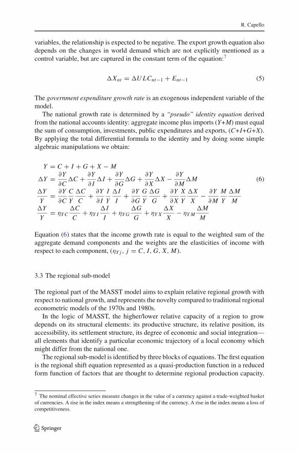
variables, the relationship is expected to be negative. The export growth equation alsodepends on the changes in world demand which are not explicitly mentioned as acontrol variable, but are captured in the constant term of the equation:7

�Xnt = �U LCnt−1 + Ent−1 (5)

The government expenditure growth rate is an exogenous independent variable of themodel.

The national growth rate is determined by a “pseudo” identity equation derivedfrom the national accounts identity: aggregate income plus imports (Y+M) must equalthe sum of consumption, investments, public expenditures and exports, (C+I+G+X).By applying the total differential formula to the identity and by doing some simplealgebraic manipulations we obtain:

Y = C + I + G + X − M

�Y = ∂Y

∂C�C + ∂Y

∂ I�I + ∂Y

∂G�G + ∂Y

∂ X�X − ∂Y

∂ M�M (6)

�Y

Y= ∂Y

∂C

C

Y

�C

C+ ∂Y

∂ I

I

Y

�I

I+ ∂Y

∂G

G

Y

�G

G+ ∂Y

∂ X

X

Y

�X

X− ∂Y

∂ M

M

Y

�M

M�Y

Y= ηY C

�C

C+ ηY I

�I

I+ ηY G

�G

G+ ηY X

�X

X− ηY M

�M

M

Equation (6) states that the income growth rate is equal to the weighted sum of theaggregate demand components and the weights are the elasticities of income withrespect to each component, (ηY j , j = C, I, G, X, M).

3.3 The regional sub-model

The regional part of the MASST model aims to explain relative regional growth withrespect to national growth, and represents the novelty compared to traditional regionaleconometric models of the 1970s and 1980s.

In the logic of MASST, the higher/lower relative capacity of a region to growdepends on its structural elements: its productive structure, its relative position, itsaccessibility, its settlement structure, its degree of economic and social integration—all elements that identify a particular economic trajectory of a local economy whichmight differ from the national one.

The regional sub-model is identified by three blocks of equations. The first equationis the regional shift equation represented as a quasi-production function in a reducedform function of factors that are thought to determine regional production capacity.

7 The nominal effective series measure changes in the value of a currency against a trade-weighted basketof currencies. A rise in the index means a strengthening of the currency. A rise in the index means a loss ofcompetitiveness.

123


These factors, stemming from the modern theories of regional growth, without denyingthe importance of traditional growth theories are the following:8

– local material inputs and resources, like infrastructure endowment, share of self-employees, external resources like CAP (Community Agricultural Policy) funds,share of tertiary activity;

– structural and sectoral resources: quantity and quality of human capital, availabil-ity of energy resources;

– the institutional elements, like economic integration processes which provide alarger market potential for regions;

– the spatial and territorial structure, the former captured through the relative geo-graphical position, which emphasises growth opportunities of a region dependenton its neighbouring regions’ dynamics (spatial spillovers of growth). The lattercaptured through the settlement structure of region, a good proxy to capture the roleof agglomeration and urbanisation economies on regional performance, enablingparameters of the different explicative variables to vary across different settle-ment structures present in space, again emphasising the strategic elements, likeagglomeration economies.

The differential shift equation is therefore:

sr = f (local material inputs and resources; structural and sectoral characteristics;

institutional elements, spatial and territorial structure) (7)

Not all the explicative variables are exogenous in the model; three of them are endog-enous and allow for cumulative processes, namely:

– self-employment is in part dependent on structural funds expenditures, as thecreation of new firms is viewed as one of the most productive effects of struc-tural funds expenditures (SF):

�selfemployeesr t = λ0 + λ1SFr t (8)

– demographic changes (population growth rate �Prt ) are dependent on birth (fr)and death rates (mr) and on in-migration (im):

�Prt = λ0 + λ1frr t−1 + λ2mrt−1 + λ3imr t−1 (9)

– that part of regional growth dependent on the other regions’ dynamics (spatialspillovers) is dependent on the regional growth of neighbouring regions in the

8 Recent new textbooks have been published which provide a new approach to regional growth, namely,Capello (2007), Pyke et al. (2006).

123

R. Capello

previous year:9

SPr t =n∑

j=1

�Y jt

dr j(10)

�Y jt = income growthj = all neighbouring regions of region rdr j = physical distance between region r and jn = number of neighbouring regions

– a removal of institutional barrier is a dependent variable, since it is obtained asthe difference between the indicator of the growth differential with neighbouringregions and the same indicator calculated by squaring the distance for those regionsat the border between Eastern and Western Countries, as follows:

IPr t =n∑

j=1

∣∣�Y jt − �Yrt∣∣

dr j−

n∑

j=1

∣∣�Y jt − �Yrt∣∣

d2r j

; r �= j (11)

where all symbols have already been defined. This indicator was built for borderregions between the new and old member countries up to 2007 and for border regionsbetween member countries and Bulgaria and Romania after 2007. In fact, it was builtwith the aim to measure the effects of a barrier reduction on the regional GDP growthrate; in particular, it was used to measure the effects of the integration of Bulgaria andRomania in 2007, after the entrance of the two countries in the EU.

In its turn, in-migration is made dependent on regional income differentials (wet−1−wr t−1), unemployment rate (u), and on the different settlement structures of regions:

imr t = η0 + η1urt−1 + η2(wet−1 − wr t−1) (12)

where:we = European average wagewr = regional average wage

9 An indicator weighting each regional growth rate for the share of each regional economy (GDP) onthe European total GDP was calculated in addition to the non-weighted one. A high statistical correlationemerged between the two, (Pearson’s correlation coefficient = 0.93). Moreover, the difference between thetwo standardised indices showed a low spatial autocorrelation, with Moran’s I index of 0.30. By removing afew outliers (mainly a few Nordic and Spanish regions), the resulting Moran’s I index equaled 0.18. On thebasis of this correlation, the decision to use the non-weighted spillover indicator was made given its highersimilarity with the classic spatially-lagged models of spatial econometrics. This indicator is an economicpotential measure, which is generally calculated as the accessibility to total income at any location allowingfor distance, following Clark et al. (1969). Here the concept is attributed to accessibility to the incomegrowth rate.

123


Table 2 Logic of the simulation procedure

Forecasts Year t Year t+1 (and following)

Estimated national growth

(At) Calculation of actual national growth with the national sub-model (output of MASST in time t)

(At+1) Calculation of actual national growth with the national

model, as a function of lagged potential growth (output of MASST in t+1)

(Bt) Calculation of regional differential shift with the regional sub-model

(Bt+1) Calculation of regional differential shift with the regional model

Estimated regional growth

(Ct) Actual regional growth is calculated as the sum of A and B, where B is rescaled to have 0 mean within each country (output of MASST in time t)

(Ct+1) Regional growth is calculated as the sum of A and B,where B is rescaled to have 0 mean within each country (output of MASST in t+1)

t) Potential regional growth is equal to the sum of A and B (non rescaled). Potential national growth is equal to the increase in the sum of potential regional income levels in Dt

(Dt+1) Potential regional growth is equal to the sum of A and B (non rescaled). Potential national growth is equal to the increase in the sum of potential regional income levels in Dt+1

(D

The last year available by official statistics at the beginning of the estimations was 2002

3.4 The simulation algorithm

The way in which the recursive mechanism works over time in a forecasting model isof great importance for the full understanding of the logic hidden behind the simulationprocedure.

In the case of MASST model, the simulation algorithm has a particular role, thatof creating a “generative” process of regional growth. In other words, our intentionwas to create a model in which regional dynamics play an active role in explainingnational growth, and do not derive only from distributive mechanisms of allocation ofnational growth.

A conceptual difference between ex-post and ex-ante national growth can be useful,and finds an operational treatment in MASST. Ex-post national growth rates can benothing else than the weighted sum of regional growth rates. If an ex-post, competi-tive approach to growth is chosen, the regional blocks of equations play only the roleof distributing national growth among the regions of the country. On the contrary, ifan ex-ante, generative, approach is chosen, the possibility exists that national growthcould be obtained thanks to the performance of the single regions; in this case, regionalgrowth plays an active role in defining national growth.

Our conceptual and operational approach follows the second definition: in MASST,the regional sub-model explains in part the national performance. Operationally,MASST treats ex-ante and ex-post growth rates as follows:

123

R. Capello

II

III

IV

III

II

INational shocks

Nation

Region i Region j

Regional shocks

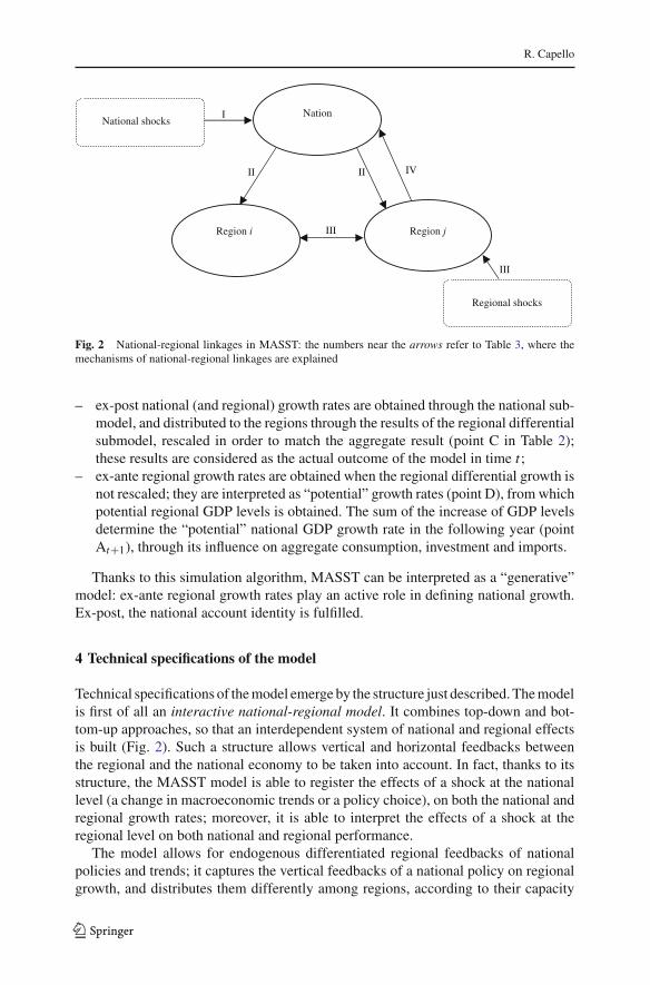
Fig. 2 National-regional linkages in MASST: the numbers near the arrows refer to Table 3, where themechanisms of national-regional linkages are explained

– ex-post national (and regional) growth rates are obtained through the national sub-model, and distributed to the regions through the results of the regional differentialsubmodel, rescaled in order to match the aggregate result (point C in Table 2);these results are considered as the actual outcome of the model in time t ;

– ex-ante regional growth rates are obtained when the regional differential growth isnot rescaled; they are interpreted as “potential” growth rates (point D), from whichpotential regional GDP levels is obtained. The sum of the increase of GDP levelsdetermine the “potential” national GDP growth rate in the following year (pointAt+1), through its influence on aggregate consumption, investment and imports.

Thanks to this simulation algorithm, MASST can be interpreted as a “generative”model: ex-ante regional growth rates play an active role in defining national growth.Ex-post, the national account identity is fulfilled.

4 Technical specifications of the model

Technical specifications of the model emerge by the structure just described. The modelis first of all an interactive national-regional model. It combines top-down and bot-tom-up approaches, so that an interdependent system of national and regional effectsis built (Fig. 2). Such a structure allows vertical and horizontal feedbacks betweenthe regional and the national economy to be taken into account. In fact, thanks to itsstructure, the MASST model is able to register the effects of a shock at the nationallevel (a change in macroeconomic trends or a policy choice), on both the national andregional growth rates; moreover, it is able to interpret the effects of a shock at theregional level on both national and regional performance.

The model allows for endogenous differentiated regional feedbacks of nationalpolicies and trends; it captures the vertical feedbacks of a national policy on regionalgrowth, and distributes them differently among regions, according to their capacity

123


Table 3 Measurement methods of interactive national-regional linkages

Effects

Shocks National Regional

National I II

National effects measured throughdynamic national income growthpresent in the estimation proce-dure

Regional effects measured throughthe national component inregional growth compoundedby regional growth spillovers andterritorial dummies present in theestimation procedure

Regional IV III

National effects measured throughthe national income growthobtained as an increase in re-gional income levels in thesimulation procedure

Regional effects measured throughthe presence of regional controlvariables and spillovers in the esti-mation procedure

to capture national growth potentialities (regional growth spillovers, settlement struc-ture). Table 3 presents the way in which these linkages take place. National shocksare registered on national GDP growth rates through the national GDP growth presentin the consumption and import growth equations. National shocks propagate to theregional level since regional GDP growth is obtained as the sum of the national GDPgrowth and the regional differential GDP growth. The latter is distributed differentlyamong regions via spillover effects and territorial dummies.

Regional shocks, and regional feedbacks, propagate on regional GDP growth thanksto the shift equation: regional shocks differ among regions thanks to spillovers, dummyvariables and different levels of the control variables. Regional shocks propagate tothe national level through the sum of the regional GDP levels which defines the annualnational GDP growth. This feedback is the only one which takes place in the simulationand not in the estimation procedure.

Moreover, the MASST model is an integrated model. In its structure, the model findsa specific place for both socio-economic and spatial (horizontal) feedbacks amongregional economies. While the former are captured by the socio-economic conditionsgenerating interregional migration flows, the latter are measured by spatial spillovereffects, the growth rate of a region being also dependent on the growth rate of itsneighbouring regions.

MASST does not confine its explanation of regional growth to economic materialresources alone: two elements of a different nature play an important role in deter-mining regional growth in the model, relational and spatial elements. In MASST,regional growth is in fact also conceived as a relational and a spatial process: demo-graphic (population growth and migration flows) and territorial tendencies performan important role in the explanation of regional growth differentials. In the case ofrelational elements one has to admit that the data unavailability hampers the full empir-ical analysis of this dimension, at present replaced by socio-demographic phenomena,like migration; it is nevertheless important to stress theoretically its importance and

123

R. Capello

suggest that data be collected in this area at regional level in the future. The spatialand territorial dimensions have a role in the explanation of regional growth in twoways. First of all, the model directly captures proximity effects through the measure-ment of spatial spillovers; moreover, with the introduction of variables interpretingthe territorial (agglomerated, urbanised, rural) structure, the model indirectly measuresthe agglomeration economy (diseconomy) effects that influence growth (decline) ina cumulative way. Spillover variables enter the differential growth equation on theirown and crossed with territorial variables, in order to capture spillovers that may occurbetween complimentary territorial structures that are not proximal.

Another important feature of the model is that it is an endogenous, local competi-tiveness driven model in the explanation of regional growth, as we expected it to be.Regional growth is explained by local factors and interregional competitiveness stemsfrom specific locational advantages and resource endowment.

MASST is a macroeconomic (multinational) model. Short-term (macroeconomic)effects are dealt with at the national level, and their feedbacks on national and regionaleconomies are taken into consideration in explaining local dynamic patterns.

MASST is a dynamic model. The outcome of one period of time at both nationaland regional level enters the definition of the output of the following period, in acumulative and self-reinforcing development pattern.

As already noted above, MASST is a generative regional growth model, in whichregional performance influences national growth patterns. This feature is what distin-guishes the model from the ones present in the literature.

Given the above characteristics, the model is a multi-layer, policy impact assess-ment model. The structure of the model allows it, in fact, to measure the impact ofnational (and supranational) policy instruments on both regional and national growth,and the impact of regional policies on national and regional growth.

5 The national and regional datasets

5.1 Description of data

No major problems exist in the collection of national level data. The national dataused in our model come from the Eurostat database, which presents a rich collection ofnational data including macroeconomic variables, in time series for all European coun-tries. Table 4 presents the indicators built for our model, available annually between1995 and 2002 for the 27 countries. The series do not go further back in time becausedata for Eastern countries are in fact available in a consistent way only since 1995.A set of dummy variables identifying new member countries has easily been built andadded to the dataset.

Most of the national data come from the Eurostat database—as most economic dataincluded in the Espon database—and taken at ESA95.

At the regional level, the availability of data is very different. As is often the case,data availability represents one of the main constraints for regional econometric modelapplications. Our case is not an exception in this respect. The main novelty concern-ing data have been the existence of the ESPON database, containing interesting and

123


Table 4 Variables used by the MASST at national level

National variables Defintions Period covered Source of(NUTS0 level) raw data

GDP growth rate Annual % growth rate of real GDP 1995–2002 Eurostat

Annual change in interest rate Absolute change in short-term inter-est rates (3 months)

1995–2002 Eurostat

Annual change in unit labour cost Absolute change in unit labour cost(calculated as unit salary × num-ber of employees / GDP)


Share of FDI on total internalinvestments

Flow of FDI / gross fixed capitalformation

1995–2002 OECD

Exchange rate Nominal effective exchange ratecalculated on 41 countries(NEER41)


Inflation rate Inflation rate (% change of CPI) 1995–2002 Eurostat

Consumption growth % annual real consumption growthrate


Investment growth % annual real gross fixed capital for-mation growth rate


Import growth % annual real import growth 1995–2002 Eurostat

Eastern countries All former Eastern Economies Dummy

New EU countries The 10 new Member Countries whojoined the EU on the 1/5/04

Dummy

unusual data at NUTS2 and NUTS3 regions, collected by research partners within thedifferent ESPON projects.

The originality of our database consists in: (a) specific and so far unavailable ter-ritorial and socio-economic data; (b) specific spatial effects indicators, built in orderto capture proximity effects, in keeping with the large and accepted literature on thisissue;10 (c) a merged Eurostat and ESPON economic data base, which enabled fillinggaps and checking for data consistency.

(a) Specific and so far unavailable territorial and socio-economic data

The new and original territorial variables are (Table 5):

– a typology of regions according to their settlement structure. Regions are in factdivided into agglomerated, urban and rural regions, on the basis of the type ofurban system (dimension and density of cities) present in the region (Fig. 3);

– a typology of best performing regions, defined MEGAs (Metropolitan EuropeanGrowth Areas), selected on the basis of five functional specialisation and perfor-mance indicators: population, accessibility, manufacturing specialisation, degreeof knowledge and distribution of headquarters of top European firms. All of thesevariables were collected at the FUA (Functional Urban Area) level and combined

10 See among others Cheshire (1995), Cheshire and Carbonaro (1996), and the wide literature on spatialeconometrics. On the latter, see, among others, Anselin (1988), Anselin and Florax (1995).

123

R. Capello

Table 5 Territorial and social and economic data so far unavailable

Data Definition Source of raw data

Agglomerated regions With a centre of >300,000 inhabitantsand a population density >300 inhab-itants / km sq. or a population density150–300 inhabitants / km sq.

Espon database

Urban regions With a centre between 150,000 and300,000 inhabitants and a populationdensity 150–300 inhabitants / km sq.(or a smaller population density—100–150 inh. /km with a bigger cen-tre (>300.000) or a population densitybetween 100 and 150 inh./km sq.

Espon database

Rural regions With a population density <100/km sq.and a centre >125,000 inh. or a pop-ulation density < 100/km sq. with acentre < 125,000

Espon database

Megas regions Regions with the location of at least oneof the 76 “Megas”—FUAs with thehighest score in a combined indica-tor of transport, population, manufac-turing, knowledge, decision-making inthe private sectors

Espon database

Pentagon regions Regions located within the Pentagonformed by the five European cities ofLondon, Paris, Milan, Munich, Ham-burg

Espon database

Net immigration flows (peoplebetween 17 and 27 years)

Average net immigration flows of peoplebetween 17 and 27 years in the period1/1/95–1/1/00 at NUTS 2

Espon database



Espon database



Espon database

Regional birth rate Share of births on population at NUTS 2in the years 1995–2001. In estimationsused 1999

Espon database

Regional mortality rate Share of deaths on population at NUTS 2in the years 1995–2001. In estimationsused 1999

Espon database

Energy consumption Share of energy toe (tons oilequivalent) on 1,000 inhabitants atNUTS 0 1990–2002. Estimations atNuts 2 made as report in notea.

Our estimation fromnational data ofESPON 2.1.4

Energy price elasticityb % change in GDP due to 10% change inenergy price

Espon 2.1.4 project

a Regional energy consumption has been estimated by distributing total national consumption to regionson the basis of a weighted sum of regional km made by car (weight = 0.15), by train (weight = 0.35) andby plane (weight = 0.5) in 2001 and of the share of populationb The energy price elasticity is an estimated data. The estimation procedure can be found in the final reportof ESPON project 2.1.4 available on the Espon website (http://www.espon.eu), pp. 135–145

123


Settlement typesRuralUrbanAgglomerated

Fig. 3 Settlement structure of European regions

to give an overall ranking of FUAs; the 76 FUAs with the highest average scorehave been labelled MEGAs (Fig. 4). 11 MEGA regions are the NUTS2 level admin-istrative areas with at least one of the 76 FUAs located in it;

– a definition of Pentagon regions, indicating the regions located within the Penta-gon area delineated by the five European cities of London, Paris, Milan, Munich,Hamburg.

The socio-economic variables collected by the ESPON projects, which would beotherwise unavailable at NUTS 2 level, are found in (Table 5):

– total energy consumption, obtained by summing the different sources of energyconsumption (travel, industrial and domestic use), once estimated at national levelthrough an input–output model, and distributed among regions according to theweighted sum of regional km traveled by car, by train and by plane in 2001 and tothe share of population;

11 See ESPON project 1.1.1. for technical details, available on the Espon web-site http://www.espon.lu.

123

R. Capello

Regions with Megas

Fig. 4 Mega regions in Europe

– energy price elasticity, as percentage change in GDP due to 10% change in energyprice;

– interregional and international migration flows, for different population age;– birth and death rates;– structural funds expenses;– agricultural support funds, divided into Pillar 1 and 2 of CAP.

(b) Specific spatial effects indicators

Specific indicators for spatial effects concern:

– a spatial spillover indicator for a generic region r , capturing an economic potential(Clark et al. 1969) as the sum of the annual absolute difference between incomegrowth rates of all other regions j divided by the distance between each region rand region j , defined in Eq. (10):

– a European integration potential indicator for a generic region r , obtained asdescribed in Eq. (11).

123


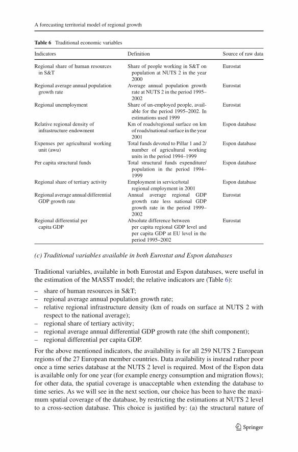
Table 6 Traditional economic variables

Indicators Definition Source of raw data

Regional share of human resourcesin S&T

Share of people working in S&T onpopulation at NUTS 2 in the year2000

Eurostat

Regional average annual populationgrowth rate

Average annual population growthrate at NUTS 2 in the period 1995–2002

Eurostat

Regional unemployment Share of un-employed people, avail-able for the period 1995–2002. Inestimations used 1999

Eurostat

Relative regional density ofinfrastructure endowment

Km of roads/regional surface on kmof roads/national surface in the year2001

Espon database

Expenses per agricultural workingunit (awu)

Total funds devoted to Pillar 1 and 2/number of agricultural workingunits in the period 1994–1999

Espon database

Per capita structural funds Total structural funds expenditure/population in the period 1994–1999

Espon database

Regional share of tertiary activity Employment in service/totalregional employment in 2001

Espon database

Regional average annual differentialGDP growth rate

Annual average regional GDPgrowth rate less national GDPgrowth rate in the period 1999–2002

Eurostat

Regional differential percapita GDP

Absolute difference betweenper capita regional GDP level andper capita GDP at EU level in theperiod 1995–2002

Eurostat

(c) Traditional variables available in both Eurostat and Espon databases

Traditional variables, available in both Eurostat and Espon databases, were useful inthe estimation of the MASST model; the relative indicators are (Table 6):

– share of human resources in S&T;– regional average annual population growth rate;– relative regional infrastructure density (km of roads on surface at NUTS 2 with

respect to the national average);– regional share of tertiary activity;– regional average annual differential GDP growth rate (the shift component);– regional differential per capita GDP.

For the above mentioned indicators, the availability is for all 259 NUTS 2 Europeanregions of the 27 European member countries. Data availability is instead rather pooronce a time series database at the NUTS 2 level is required. Most of the Espon datais available only for one year (for example energy consumption and migration flows);for other data, the spatial coverage is unacceptable when extending the database totime series. As we will see in the next section, our choice has been to have the maxi-mum spatial coverage of the database, by restricting the estimations at NUTS 2 levelto a cross-section database. This choice is justified by: (a) the structural nature of

123

R. Capello

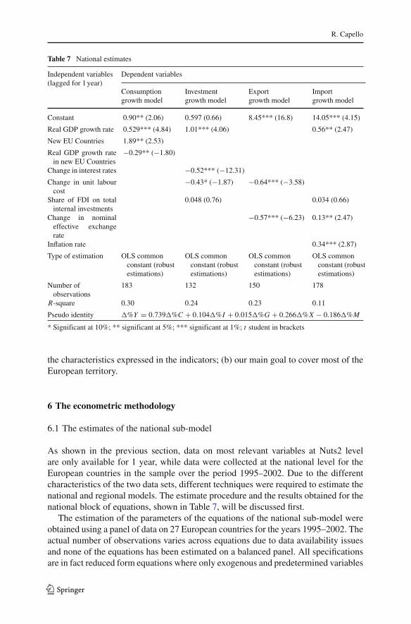
Table 7 National estimates

Independent variables Dependent variables(lagged for 1 year)

Consumption Investment Export Importgrowth model growth model growth model growth model

Constant 0.90** (2.06) 0.597 (0.66) 8.45*** (16.8) 14.05*** (4.15)

Real GDP growth rate 0.529*** (4.84) 1.01*** (4.06) 0.56** (2.47)

New EU Countries 1.89** (2.53)

Real GDP growth ratein new EU Countries

−0.29** (−1.80)

Change in interest rates −0.52*** (−12.31)

Change in unit labourcost

−0.43* (−1.87) −0.64*** (−3.58)

Share of FDI on totalinternal investments

0.048 (0.76) 0.034 (0.66)

Change in nominaleffective exchangerate

−0.57*** (−6.23) 0.13** (2.47)

Inflation rate 0.34*** (2.87)

Type of estimation OLS commonconstant (robustestimations)

OLS commonconstant (robustestimations)



Number ofobservations

183 132 150 178

R-square 0.30 0.24 0.23 0.11

Pseudo identity �%Y = 0.739�%C + 0.104�%I + 0.015�%G + 0.266�%X − 0.186�%M

* Significant at 10%; ** significant at 5%; *** significant at 1%; t student in brackets

the characteristics expressed in the indicators; (b) our main goal to cover most of theEuropean territory.

6 The econometric methodology

6.1 The estimates of the national sub-model

As shown in the previous section, data on most relevant variables at Nuts2 levelare only available for 1 year, while data were collected at the national level for theEuropean countries in the sample over the period 1995–2002. Due to the differentcharacteristics of the two data sets, different techniques were required to estimate thenational and regional models. The estimate procedure and the results obtained for thenational block of equations, shown in Table 7, will be discussed first.

The estimation of the parameters of the equations of the national sub-model wereobtained using a panel of data on 27 European countries for the years 1995–2002. Theactual number of observations varies across equations due to data availability issuesand none of the equations has been estimated on a balanced panel. All specificationsare in fact reduced form equations where only exogenous and predetermined variables

123


enter as regressors. In particular, the lagged income variable is considered to be apredetermined variable that proxies current income growth, so that we are able toavoid dealing with simultaneity issues that would arise if we used the current incomeas a regressor in the consumption, investment and imports equations. After testingfor the presence of individual effects, for the presence of serial correlation withineach individual (country) and for heteroskedasticity, all equations ended up beingestimated by robust OLS that ensure consistent but not necessarily efficient estimatesof the parameters. Comments on each equation follow.

(a) The consumption equation (see Table 7, column 2)

Theory tells us that consumption depends primarily on income. Which among past,current or expected income is the “right” measure to use in a consumption equationis both a theoretical and empirical issue, and there has been a considerable amountwritten on this topic. In MASST, we choose to specify and estimate the aggregategrowth rate of consumption as a linear function of the lagged aggregate income growthrate, allowing for different coefficients between the old and the new EU members,12

as well as a dummy that changes the intercept of the equation for the new EU mem-ber countries. We estimate the consumption equation by ordinary least squares (OLS)on a panel of data from 1996 through 2002 for the 27 European countries in thesample.13

Neither fixed nor random individual effects were found statistically significant, andthis allowed us to use OLS rather than panel specific estimation techniques. We testedfor serial correlation within each country in the OLS residuals and we accepted thenull hypothesis of no serial correlation, which we took as support of taking the laggedincome growth variable as a predetermined variable.

We did not test for spatial correlation in the residuals of the consumption equationbut we decided to estimate robust standard errors of the parameters of the equationto ensure that we were able to make correct statistical inferences on the parametersthemselves even if the error terms were heteroskedastic or somehow correlated acrossobservations.14

The estimation process shows that consumption follows significantly different pat-terns of behaviour between old and new EU member countries. In particular the growthrate of consumption is on average greater in the new countries, while the marginal rateof consumption relative to income is larger for the old countries: the latter save lessand they have already reached an almost steady state consumption growth rate.

12 In this equation Bulgaria and Romania are added to the set of the 10 new EU members, despite theirentrance into the EU took place only, January 1, 2007.13 For some of those countries data are only available from 1998.14 See the “robust” option in the STATA command “regress”. Such an option produces the so called “sand-wich coefficient covariance matrix” which is a consistent estimate of the coefficient covariance matrix evenwhen there exists heteroskedasticity or correlation among residuals.

123

R. Capello

(b) The investment equation (see Table 7, column 3)

From a standard keynesian approach, aggregate investment depends positively onaggregate demand, i.e., income, (both current and expected), and negatively on inter-est rates, a proxy for cost of capital. The literature on investment equations is at leastas wide as the literature on consumption,15 but once again in MASST a simple speci-fication was chosen: aggregate investment growth is a traditional linear function of thelagged income growth and of the nominal (three months) interest rate, but also of thelagged unit labor costs growth and of the amount of FDI’s received by Eastern Euro-pean countries. The latter variable is not significant, but it has the expected positivesign: foreign direct investments push domestic investments.

On the other hand, the negative and significant coefficient of the unit labour costvariable shows that as labour costs grow investments decline, which means that labourand capital are complementary rather than substitutes. These estimations capture thefact that the countries where labour costs are low and slow-rising are the countrieswhere investments are growing at a faster rate in the years 1996–2002. The coefficientsattached to lagged income and interest rates are highly significant and of the expectedsign. Interest rates are lagged one year and are considered a predetermined vari-able; they will be treated as an economic policy instrument when devising simulationscenarios.

The same tests were performed on the estimated residuals of the investmentequation as on the consumption equation, with the same results. In particular no indi-vidual effects were found significant and robust pooled OLS were used to estimatethe coefficients and their standard errors.

(c) The exports equation (see Table 7, column 4)

In standard Keynesian demand driven macro models, exports are taken as exogenous,that is they are only determined by the demand of the rest of the world. We prefer tomodel exports as a function of supply as well as of demand factors, in particular asa function of internal competitiveness as measured by both unit labour costs and theexchange rate. A decrease in competitiveness (i.e., an increase in unit labour costs)will slow down exports and so will an increase in the nominal effective exchangerates. The constant in the equation of aggregate export growth may be interpreted asthe effect of the average demand growth of the rest of the world.

The estimation was executed using robust pooled OLS on a sample that excludedsome outlier observations, mainly relative to Romania before 1999, where and wheninflation rose to three digit values.

(d) The imports equation (see Table 7, column 5)

Aggregate import growth depends positively and significantly on lagged incomegrowth, on inflation, and on changes in the exchange rate: imports increase if internal

15 See Jorgenson (1971), and more recently Galeotti (1996), for a review of the literature on investmentequations.

123


demand grows, if domestic prices increase (and domestic goods are substituted for byimported goods), and if the nominal effective exchange rate increases.16 There is mod-est evidence that FDI’s finance imports in Eastern European countries (the coefficientattached to FDI is positive but not significant).

In MASST inflation and exchange rates are not endogenously modelled and areactually taken as exogenous variables under the assumption that they are economicpolicy instruments controlled by national or supranational authorities.

The parameters of this equation were estimated using robust pooled OLS.

(e) The “pseudo” identity (see Table 7, last raw)

The last equation in the national model is the national accounts identity expressedin the growth rates of both GDP and aggregate demand components. The estimatedcoefficients measure the average elasticity of GDP to each aggregate demand compo-nent, over all countries in the sample for years 1996 through 2002. As expected theelasticity is close to 80% for consumption, while it is approximately 18% though withopposite signs, for exports and imports. The elasticity of GDP to public expenditure isvery small: this is a result that probably depends on the tight fiscal policies that mostof the countries in the sample followed during the time period when the data werecollected, so that public expenditure contributed little to the economic growth of eachcountry.

6.2 Regional estimates

The approach followed to estimate the parameters in the regional block of equationswas mostly determined by data availability problems. Some of the variables neededto estimate the differential regional growth equation and the population and migrationequations are available for almost all 259 regions in our sample for years 1995 through2002. However, some other relevant variables, such as human capital or accessibilityand infrastructure measured through the kilometers of available roads in regions, areavailable only for 1 year, 2000 in most cases. Lastly, some territorial variables areconstant through time because of their nature (Table 8). Thus, it was not possible touse panel techniques. We chose to estimate all equations in the regional block in onecros-section, on 259 regions in one year. As it will be clearer later in the paper, theinformation along the time dimension, whenever available, was not omitted, but ithas been used to solve some specification and strictly econometric problems relatingto the possible correlation between some of the regressors and the error term of theequations and to the likely presence of spatial correlation in the estimated residuals.17

16 Nominal effective exchange rates measure changes in the value of a currency against a trade-weightedbasket of currencies. A rise in the index means a strengthening of the currency, hence a loss in competitive-ness. The index is calculated as a weighted geometric average of the bilateral exchange rates against thecurrencies of 41 competing countries. The weights use information on both exports and imports throughout.The import weights are the simple shares of each partner country in total euro-zone imports from partnercountries. Exports are double-weighted in order to account for the so-called “third market effects”.17 See Anselin (1988).

123

R. Capello

Table 8 List of variables in the regional differential shift equation

Classification Type Definition

Regional economic resources

Share of human resources in S&T Predetermined % of people working in S&T onpopulation at NUTS 2 in the year2000

Average population growth rate(1995–2002)

Predetermined Average annual population growthrate at NUTS 2 in the period 1995–2002

Energy consumption bypopulation in 2002

Predetermined Total energy consumption onpopulation at NUTS 2 in the year2002

Regional structural and sectoral characteristics

Relative density of infrastructureendowment in 2001

Predetermined (intermedi-ate policy target)

Km of roads on surface at NUTS 2on km of roads on surface at NUTS0 in the year 2001

Share of self-employment Predetermined Share of self-employment on totalemployment

Share of tertiary activity in 2001 Predetermined (intermedi-ate policy target)

Employment in services in 2001 inpercentage of the total at NUTS 2

Territorial specificities Dummy variables Rural, urban, agglomerated, megas

Pillar 2 expenses of CAP Policy instrument Total funds devoted to Pillar 2 onagricultural working units (awu)

Structural funds expenditures Policy instrument Total structural funds expendituresin the period 1994–1999 on popu-lation

Spatial processes

Spatial spillovers (1997–1998) Predetermined Sum of the relative annual regionalgrowth rates of all regions j otherthan region r divided by thedistance between each otherregion and region r (see Eq. 10)

European integration process

Regional integration potentials(1998–1999)

Predetermined A European integration potentialindicator for a generic region r ,obtained as the difference betweenthe indicator of growth differ-ential with neighbouring regionsdescribed above and the sameindicator calculated by squaringdistance for those regions at theborder between Eastern and West-ern Countries (see Eq. 11)

All equations have been tested for spatial dependence using the spatial regressionand testing modules in STATA,18 and a distance matrix consisting of the distances inkilometres between all couples of regions in the sample.

18 See Pisati (2001), pp. 277–298.

123


Table 9 Estimates of the regional differential shift

Independent variables Dependent variable : regional averageannual differential GDP growth rate1999–2002

Constant −5.25 (−3.93)

Economic resources

Regional share of human resources in S&T in urban areasin 2001

−0.012 (−0.5)

Regional share of human resources in S&T in EasternCountries in 2001

0.075 (4.51)***

Regional average population growth rate (1995–2002) 0.646 (3.29)***

Regional energy consumption by population in 2002 0.0067 (2.48)**

Regional energy consumption by population in tertiaryregions in 2002

−0.000111 (−4.1)***

Structural and sectoral characteristics

Relative regional density of infrastructure endowment in 2001 −0.13 (−0.90)

Relative regional density of infrastructure endowmentin mega areas in 2001

0.12 (0.8)

Regional share of self-employees 0.045 (2.75)***

Regional share of tertiary activity in 2001 0.058 (4.40)***

Dummy for mega regions 0.52 (2.24)**

Dummy for rural regions −0.56 (−1.37)

Pillar 2 expenses per agricultural working unit (awu) 0.03 (3.18)***

Spatial processes

Spatial spillovers(1997–1998)

91.23 (1.72)*

Spatial spillovers in the agglomerated regions (1997–1998) −88.37 (−2.42)**

Spatial spillovers in urban areas in Eastern Countries(1997–1998)

−98.69 (−2.27)**

European integration process:

Regional integration potentials in Western Countries(1998–1999)

14.2 (0.47)

Regional integration potentials in Eastern Countries(1998–1999)

−29.02 (−0.65)

Number of observations 227

R-square 0.30

Spatial error test: robust Lagrange multiplier (P value) 0.168 (0.68)

Spatial lag test: robust Lagrange multiplier (P value) 0.36 (0.54)

* Significant at 10%; ** significant at 5%; *** significant at 1%

In only one equation, the young workers net immigration equation (see later on),were the residuals characterized by spatial dependence, and the appropriate maximumlikelihood estimation technique needed to be used. For all other equations robust OLSestimates were performed.

6.2.1 The regional growth differential equation (see Table 9)

As explained in the overall description of MASST, this equation is a quasi productionfunction where potential regional output is determined by factors such as economic

123

R. Capello

and human resources, structural and sectoral characteristics, spatial processes, inte-gration processes and territorial specificities. More precisely, the dependent variablein this equation is regional “shift” sr , presented in Eq. (1).

In Table 7 all the relevant explanatory variables are presented and classified. Table 8presents the estimated specification, discussed in more detail in the following points:

– regional GDP at constant prices is available for years 1995 through 2002 for mostregions, and GDP growth rates and regional shift (sr ) from 1996 on. Yearly growthrates measure, by definition, only short term fluctuations, while our intention is infact to explain the structural part of regional growth, due to structural elements,like human capital, infrastructure endowment, population growth, the settlementstructures and agglomeration economies. Therefore, the choice of the averageregional-national differential GDP growth between 1999 and 2002 was chosen asthe dependent variable, so as to smooth out any abnormal short-term fluctuationsin regional income;

– while dealing with production functions, we must acknowledge that output andproduction factors are actually jointly determined: output is a function of pro-duction factors, but the latter are demanded by firms as a function of (planned)output (as well as of factor prices). In econometric terms, production factors usedas regressors in a production function will be correlated with the error term ofthe equation, and induce inconsistent parameter estimates. For this reason, in theregional shift equation the lagged in time proxies of the production factors wereintroduced whenever possible. Labour growth rate, for instance, is proxied by theaverage population growth rate between 1995 and 1998; this regressor may bedefined as a predetermined variable and will not be correlated with the error termin the equation, that we assume to be serially independent;19

– unfortunately, for other production factors and sectoral characteristics (share oftertiary employment, for example) only data on year 2000 are available (one of theyears used to compute the dependent variable). In this case, the assumption is madethat their volume, although measured for year 2000, was actually determined byprevious years’ incomes and activity levels. Thus, also these variables are treatedas predetermined variables and are assumed to be uncorrelated with the error termin the equation;

– the growth spillover and integration potential variables are computed for eachregion/observation as weighted averages of the income growth rates of the otherregions in the sample, using as weights the distances between each couple ofregions (Formulas 10 and 11). Spatial econometrics proves that regional growthrates are jointly determined and these spatially lagged regressors will be contem-poraneously correlated with the error term. To avoid this simultaneity problem,and given the availability of data on regional income for years before 1999, thegrowth spillover and potential integration variables were computed on lagged intime income growths. In econometrics terms, this operation allows the use of OLSto estimate the parameters of this equation, once again relying on the property of

19 It is not possible to test for serial correlation within each region, given that, with the available data, wecan only estimate one cros-section in time.

123


consistency of OLS estimators that holds when regressors and error term are notcontemporaneously correlated and error terms are not serially correlated. From aneconomist’s perspective, using lagged in time spillover and integration potentialvariables as regressors introduces a dynamic component into the specification thatmay yield useful information on the speed of adjustment of each region’s growth toneighbouring regions’ growth, and on how such speed may be affected by territorialcharacteristics. In fact these lagged in space and lagged in time spillover variablesenter the differential growth equation on their own and crossed with territorial vari-ables (see Table 9). Both these elements, the introduction of time dynamics intothe specification and the possibility to estimate the effects of spillovers crossedwith territorial variables, were the reason we chose to compute our own spilloverand integration potential variables instead of using the available spatial regressionpackages that automatically compute the spatially lagged variable and estimate bymaximum likelihood the spatial lag model in one point in time;20

– tests for spatial dependence were run and the null hypothesis of no spatial corre-lation in the error terms was not rejected. The model was estimated with robustOLS.

Table 9 shows the estimation results. R2 of the equation is 0.3, not large indeed inabsolute terms, but more than acceptable given the growth rate specification of theexplanandum: it is worth remembering that the dependent variable in this equation isa difference in growth rates, almost a random variable itself. The coefficients of mostof the relevant variables are however statistically significant.

From the economic point of view, the model suggests that regional competitive-ness finds its roots in the presence of: (a) structural and sectoral features; (b), localeconomic resources; (c) spatial and territorial structure and (d) institutional elementspresent in the “border regions” effect on the integration potential.

(a) Structural and sectoral features

The relative infrastructure endowment coefficient has a negative and non-significantsign. The conclusion of this result is that in general better infrastructure endowmentwith respect to the national average does not necessarily result in a greater compet-itiveness of the local economy. Interestingly enough, results change in terms of signwhen infrastructure endowment is related to the mega regions. In these regions a richinfrastructure endowment helps to keep the decreasing returns and the inefficiency ofa highly congested infrastructure context under control.

In terms of sectoral structure, the model proves that the share of tertiary activityin a region explains its differential growth; the coefficient of this variable shows apositive and significant sign. This result supports the empirical evidence that highercompetitive gains stem from tertiary rather than industrial activities.

Another interesting result is the role played by agricultural support funds, and inparticular by Pillar 2 expenses in agriculture, i.e., those directly supporting productionand productivity, while, as easily explainable, Pillar 1 agricultural expenses, devoted

20 See fore example the module “spatreg” in STATA, with the spatial lag option.

123

R. Capello

to the support of farmer income (rather than production), proved to have no impact onregional growth of GDP.

(b) Local economic resources

The presence of a high quality of human capital proved once again to be an importantelement explaining local competitiveness in areas where the initial level of qualified hu-man capital is low, like in Eastern Countries; the non-rival and partially non-excludablenature of a part of the outcome of knowledge creation, as theorised in Romer’s endog-enous growth model (Romer 1986), induces more knowledge generation, and createsdynamic increasing returns in the form of a faster growth rate. Our results prove how-ever that the knowledge spillover effects are accompanied by decreasing returns, inthat Eastern Country regions, characterised by a lower level of knowledge, experiencegreater relative positive effects from knowledge spillovers than highly and technolog-ically advanced urban regions.

The results witness also that human resource growth, measured in terms of pop-ulation growth, plays an important role in explaining local competitiveness. By thesame token, energy resource consumption has a positive impact on local growth. Inter-estingly enough, in tertiary activity regions the energy consumption coefficient has alower value, witnessing a more limited (though positive) effect of energy consump-tion on growth, due both to the specialisation patterns and increasing returns in energyconsumption characterising the tertiary—more concentrated—areas.

Lastly, the share of self-employment has a rather important role in explainingregional differential growth. It has a significant and positive sign, indicating thatentrepreneurship is playing a strategic role in regional growth patterns. Note that themodel specifies and estimates (see column 1 in Table 10) self-employment as affectedby structural funds decided upon jointly by European and national policy makers; thusMASST is able to analyse the effects of another relevant policy instrument on regionalgrowth.

(c) Spatial and territorial structure

The most recent literature on spatial growth gives great emphasis to spatial processes, inthe form of increasing returns, agglomeration economies, cumulative self-reinforcingprocesses and spatial spillovers. The results of the model witness that these processesdo have an effect on regional differential growth, and are in general positive; a fastergrowing area spreads around its positive effects, and stimulates local production andgrowth of its neighbouring regions.

A striking effect takes place when spatial growth spillovers are estimated for specificterritorial areas.

In those agglomerated areas showing a greater density of productive activities andpopulation, and therefore expected to be characterised by greater dynamic agglom-eration economies, spatial spillovers are much lower, though still positive. Highlynegative spatial spillovers—i.e., backwash effects—occur instead in highly urbanisedregions in Eastern countries: faster growing regions tend to attract resources (moreproductive and highly paid workers, efficient and dynamic firms, more financial invest-

123


Table 10 Estimation of regional share of self employment and regional annual population growth equations

Independent Dependent variablesvariables

Regional share of Regional annual averageself-employment population growth rate

1996–2002

Constant 11.06 (19.5)*** −0.084 (−0.25)

Structural funds expenditures in the period1994–1999 on population

0.010 (7.31)***

Birth rate (lagged 1 year) 0.10 (6.66)***

Death rate (lagged 1 year) −0.079 (−2.98)***

Net immigration flows (people between 17and 27 years). Average value in the period1995–2000

0.012 (2.91)***

Net immigration flows (people between 32and 42). Average value in the period 1995–2000

0.0461 (4.95)***

Net immigration flows (people between 52and 67 years). Average value in the period1995–2000

−0.014 (−0.57)

New EU countries −0.33 (−4.95)**

Agglomerated regions −0.18 (−3.24)**

Number of observations 191 257

R-square 0.42 0.36

Type of estimate OLS (robust estimates) OLS (robust estimates)

Spatial error test: robust Lagrange multiplier(P value)

0.85 (0.36)

Spatial lag test: robust Lagrange multiplier(P value)

2.59 (0.108)

* Significant at 10%; ** significant at 5%; *** significant at 1%

ments) from its neighbouring regions, increasing the differential in economic growthrate with respect to them. This result is in line with other empirical studies on spa-tial effects on regional differential growth.21 Urban regions in Eastern countries growat the expenses of neighbouring regions characterised by medium cities and a ruralenvironment.

Coefficients for dummy variables concerning the mega regions and the rural regionsprove first of all to be very significant in explaining regional growth; secondly theyprove to differ substantially, in terms of sign: the sign is in fact positive for mega regionsand negative for rural areas. Through their econometric significance, these resultsconfirm the conceptual importance of territorial elements in regional growth: agglom-eration economies, present in the mega regions in the form of cumulative knowledgeand collective learning processes, play a fundamental role in a cumulative and self-reinforcing economic growth process; their absence in rural areas explain a large partof the limited economic dynamics of these territories. These results also witness the

21 See Cheshire (1995); Cheshire and Carbonaro (1996).

123

R. Capello

powerful capacity of dummy variables on the settlement structure in interpreting therole of space in regional growth.

(d) Economic integration processes

The last group of variables contained in the model measures the effects of a more inte-grated Europe. As mentioned before (Sect. 3.3), the concept of integration potentialis measured on the basis of the change taking place in the economic potential of aregion once integration and disappearance of previous political-institutional barrierstakes place.

The results are interesting but unfortunately not significant from a statistical pointof view. The signs of the coefficient suggest that the enlargement process generatesin the first stages of its implementation negative effects to the weakest regions, whichoffer a large market potential to more advanced and competitive areas; at the sametime, it generates advantages to advanced regions, able to grasp new market oppor-tunities. The integration potential coefficient has in fact a negative sign for Easterncountry regions and a positive one for Western country areas.

6.2.2 The population growth equation (See Table 10, column 2)

The last equation in the demographic block, population growth is specified as a functionof net immigration, birth and death rates and territorial variables. Note that popula-tion growth also depends, via the contemporaneous migration variables, on the laggedregional GDP. In fact, the demographic block of equations has been built along a recur-sive pattern: we assume that population depends on migration but migration does notdepend simultaneously on population growth. This very plausible assumption enablestreating the migration variables as non contemporaneously correlated with the errorterm of the population equation and to avoid simultaneity issues.

The dependent variable has been computed as the average population growthbetween 1999 and 2002 for reasons similar to those given for the choice of dependentvariable in the growth differential equation. As expected, the birth rate and death rate(lagged 1 year) have a positive and negative sign, respectively. Immigration flows ofpeople also increase the population growth rate, with the exception of the 52–67-yearage group. This has a negative impact on population growth, which finds a doubleexplanation: (a) the low fertility rate of this group; (b) the general average negative signof the variable (measuring therefore an out-migration process on average). Tenden-cies to lose population are typical of new EU Countries and of agglomerated regions;economic difficulties, physical congestion and in general agglomeration diseconomies(high land prices) explain these tendencies (Table 10).

The tests accepted the null hypotheses of no spatial dependence or spatial lag androbust OLS were used to estimate the parameters of the equation. The R2, measure ofgoodness of fit is 65%.

6.2.3 The migration equations (See Table 11)

The model contains three equations that track the pattern of net immigration by agegroup: young, middle aged and older workers. Each of the three variables depends on

123


Table 11 Estimation results of the regional immigration equations

Independent variables Dependent variables

Net immigration flows(people between 17and 27 years)

Net immigration flows(people between 32and 42)

Net immigration flows(people between 52and 67 years)

Constant 1.59 (0.51) 7.61 (8.53)*** 1.79 (1.33)

Regional differential GDP(with the EU) (lagged 1 year)

1.14 (8.07)***

Unemployment rate(lagged 1 year)

−0.73 (−4.00)*** −0.92 (−5.83)*** −0.57 (−4.72)***

Megas Regions 3.59 (2.01)**

Agglomerated Regions 5.41 (3.27)*** −2.26 (−3.34)*** −2.87 (−5.07)***

Eastern countries 15.29 (4.41)***

Regional share of tertiary activity 0.053 (2.15)**

Regional differential GDP(with the EU) (lagged 1 year)in Western countries

−0.34 (−5.56)*** −0.359 (−7.08)***

Regional differential GDP(with the EU) (lagged 1 year)in Eastern countries

0.19 (5.28)***

λ-spatial correlation coefficientin errors

− 1.4E-05(−5.63)***

Type of estimation Spatial ErrorMaximumLikelihood

OLS (robustestimates)

OLS (robustestimates)

Number of observations 244 250 250

R-square 0.27 [Squared corre-lation]

0.30 0.32

Spatial error test robustLagrange multiplier (P value)

38.43 (0.00) 0.021 (0.88) 0.097 (0.75)

Spatial error test robustLagrange multiplier (P value)

22.92 (0.00) 0.77 (0.38) 2.25 (0.13)

* Significant at 10%; ** significant at 5%; *** significant at 1%. t-student in brackets

time lagged per capita GDP differentials between the region and the average EUper capita GDP and on unemployment rates in the region. Territorial and socio-economic variables characterize each equation. After estimation, the results showthat the younger work force migrates towards agglomerated and fast growing regions.Middle aged and especially older workers, instead, migrate away from highly con-centrated and industrialized regions towards regions with a larger share of tertiaryactivities. All categories move away from areas with large unemployment rates.

Statistical evidence of spatial dependence in the error term of the young workersnet immigration equation was found, but not for the other two migration equations.Accordingly, the parameters of the young workers equation and the variation coeffi-cient of spatial dependence in the first equation were jointly estimated22 by MaximumLikelihood, while robust OLS regressions were used to estimate the parameters of theother two equations.

22 See Anselin (1999, p. 16); see also the spatreg procedure in STATA, Pisati (2001).

123

R. Capello

7 Conclusions and future research directions

The paper had the aim to present the conceptual logic of MASST as a forecastingregional growth and a policy simulation model. The characteristics of the model wereto be based on a modern interpretation of regional growth. The model is based in facton a concept of endogenous growth, highly dependent on internal structural charac-teristics of the local economy; local competitiveness drives regional growth, beingsupply side effects of growth determined at the local level. Demand effects of growthare captured at the national level, and linked to the regional effects enabling develop-ment of a combination of top-down and bottom-up approach, so that an interdependentsystem of national and regional effects is built, and vertical linkages between nationaland regional systems are taken into account.

Moreover, in its structure, the model finds a specific place for both socio-economicand spatial (horizontal) feedbacks among regional economies. While the former arecaptured by the socio-economic conditions generating interregional migration flows,the latter are measured by spatial spillover effects that are measured by the growthrate of a region that also depends on the growth rate of neighbouring regions.

It is a spatial-territorial model. The spatial and territorial dimensions have a rolein the explanation of regional growth in two ways. First, the model directly capturesproximity effects through the measurement of spatial spillovers; moreover, with theintroduction of variables interpreting the territorial (agglomerated, urbanised, rural)structure, the model indirectly measures the agglomeration economy (diseconomy)effects that influence growth (decline) in a cumulative way. In this sense, it representsa valid and modern conceptual interpretation of regional growth, which finds verygood empirical support in the estimations presented.

The model is built in order to predict new regional growth rates and new levels ofregional per capita income in the EU 27 Countries, and therefore new levels of eco-nomic territorial disparities, under different conditional hypotheses. Given the wayin which it is built, the MASST model enables forecasting future regional growthrates on the basis of a variety of driving forces of change. Macroeconomic drivingforces (like trend in the euro/$ exchange rate; trend in fiscal morality; trend in interestrates; trend in inflation rate; geo-political orientation of FDI; rebalancing of externalaccounts of large emerging countries; increase in energy price), institutional drivingforces (i.e., the future enlargement strategies such as deepening or widening of the EU;restructuring of Community Agricultural Policy; reorientation and size of structuralfunds; attitude towards East-West and North-South migration) and socio-economicand demographic driving forces (trend in fertility rate, in population aging; in savingratio; in migration patterns) can all easily be taken into consideration to provide a mapof European regional growth rates in the years to come.

References

Anselin L (1988) Spatial econometrics: methods and models. Kluwer, DordrechtAnselin L, Florax R (1995) New directions in spatial econometrics, Springer, BerlinBarro RJ, Sala-i-Martin X (1995) Economic growth. McGrow Hill, New York

123


Becattini G (1990) The Marshallian industrial district as a socio-economic notion. In: Pyke F, Becattini G,Sengenberger W (eds) industrial districts and interfirm cooperation in Italy. International Institute ofLabour Studies, Genevra, pp 37–51

Biehl D (1986) The contribution of infrastructure to regional development, Regional Policy Division, Euro-pean Community, Brussels

Camagni R (1991) Local milieu, uncertainty and innovation networks: towards a new dynamic theoryof economic space. In: Camagni R (ed) Innovation networks: spatial perspectives. Belhaven-Pinter,Londra, pp 121–144

Camagni R, Capello R (2002) Milieux innovateurs and collective learning: from concepts to measurement.In: Acs Z, de Groot H, Nijkamp P (eds) The emergence of the knowledge economy: A regionalperspective. Springer, Berlin, pp 15–45

Capello R (2007) Regional economics. Routledge, LondonCappellin R (1975) La struttura dei modelli econometrici regionali. G Econ Ann Econ July–August: 423–

452Cappellin R (1976) Un modello econometrico dell’economia lombarda. G Econ Ann Econ June: 263–290Clark C, Wilson F, Bradley J (1969) Industrial location and economic potential in Western Europe. Reg

Stud 3(2):197–212Cheshire P (1995) A new phase of urban dispersion in Western Europe? The evidence for the 1980s. Urban

Stud 32(7):1045–1063Cheshire P, Carbonaro G (1996) Urban economic growth in Europe. Urban Stud, 33(7):1111–1128Galeotti M (1996) The intertemporal dimension of neoclassical production theory. J Econ Surv 10(4):421–

460Glickman NJ (1977) Econometric analysis of regional systems. Academic, New YorkGlickman NJ (1982) Using empirical models for regional policy analysis. In: Albegov M, Andersson E,

Snickars F (eds) Regional development modelling: theory and practice. North-Holland, Amsterdam,pp 85–104

Guzzi R, Sanglier M, El Korchi D (1996) ISIS, interregional socio-industrial system: a non-linear dynamicmodelfor multi-regional economic simulation. Final Report for the Commission of European Union,w.p. U.L.B., March 1996, Bruxelles

Hewings G, Nazara S, Dridi C (2004) Channels of synthesis forty years on: integrated analysis of spatialeconomic systems. J Geogr Syst 6:7–25

Keeble D, Wilkinson F (1999) Collective learning and knowledge development in the evolution of regionalclusters of high-techology SMEs in Europe. Reg Stud 33(4):295–303

Jorgenson DW (1971) Econometric studies of investment behavior: a survey. J Econ Lit 9(4):1111–1147Lundvall B-A (1992) Introduction. In: Lundvall B-A (ed) National systems of innovation. towards a theory

of innovation and interactive learning. Pinter Publisher, London, pp 1–19Moody HL, Puffer FW (1969) A gross regional product approach to regional model building. West Econ J,

7(4):391–402Nijkamp P, Rietveld P, Snickars K (1986) Regional and multiregional economic models: a survey. Nijkamp

P (ed) Handbook of regional and urban economics. North-Holland, Amsterdam, pp 257–294Pisati M (2001) Tools for spatial data analysis. STATA Technical Bulletin Reprints, vol 10, pp 277–298Putnam RD (1993) Making democracy work: civic traditions in modern Italy. Princeton University Press,

PrincetonPyke A, Rodriguez-Pose A, Tomaney J (2006) Local and regional development. Routledge, LondonRomer P (1986) Increasing returns and long-run growth. J Pol Econ 94(5):1002–1037Stimson RJ, Stough RR, Salazar M (2005) Leadership and institutional factors in endogenous regional

economic development. Investig Reg 7:23–52Trey GI, Rickman DS, Shao G (1992) The REMI economic-demographic forecasting and simulation model.

Int Reg Sci Rev 14(3):221–254

123

a forecasting territorial model of regional growth: the masst model

Documents