a thesis submitted in partial fulfillment of the...
TRANSCRIPT
RICE UNIVERSITY
422 nm Laser
by
Clayton Earl Simien
A Thesis Submitted
in Partial Fulfillment of theRequirements for the Degree
Masters of Science
Approved, Thesis Committee:
Thomas C. Killian, ChairmanAssistant Professor of Physics andAstronomy
Randall G. HuletFayez Sarofim Professor of Physics andAstronomy
Paul A. CloutierProfessor of Physics and Astronomy
Houston, Texas
September, 2004

2
ABSTRACT
422 nm Laser
by
Clayton Earl Simien
A 422 nm laser was constructed for the purpose of studying a strontium ultra-
cold neutral plasma. Since strontium ions have atomic lines in the visible, we can
optically image the plasma via the 88Sr+ 2S1/2 → 2P1/2 transition using 422 nm light.
We produce light at this wavelength by converting infrared light at 844 nm from a
commercial semiconductor infrared diode laser via second-harmonic generation in an
semi-monolithic linear enhancement cavity. This thesis will cover the experimental
details pertaining to nonlinear optics, optical resonator design, and locking electronics
used to create a 422 nm laser.
Acknowledgments
First, I would like to acknowledge my Lord in Heaven and His Son, my Savior,
Jesus Christ for Their grace and mercy in blessing me with family, friends, and
mentors whose help has made it possible for me to complete my master’s project.
Particular, Dr. Thomas Killian, for carrying me through this project on his shoulders
of patience and expertise. Ying-Cheng Chen for his invaluable assistance. My friend,
my brother, Musie Gherbermicheal for his wisdom, encouragement, and friendship
which has been food for my soul. Finally, I would like to give a special thanks to
my family, for all their love, support, sacrifice, and struggle that has allowed me to
survive, give me purpose, and achieve this level in my education.
Contents
Abstract i
Acknowledgments ii
List of Figures v
1 Introduction 1
1.1 Ultracold Neutral Plasmas . . . . . . . . . . . . . . . . . . . . . . . . 1
1.2 Previous Ultracold Plasma Diagnostics Schemes . . . . . . . . . . . . 2
1.3 Optically Imaging an Ultracold Plasma . . . . . . . . . . . . . . . . . 3
1.4 Outline . . . . . . . . . . . . . . . . . . . . . . . . . . . . . . . . . . . 5
2 Second Harmonic Generation 6
2.1 Theory . . . . . . . . . . . . . . . . . . . . . . . . . . . . . . . . . . . 6
2.2 Phase Matching . . . . . . . . . . . . . . . . . . . . . . . . . . . . . . 7
2.3 Potassium Niobate . . . . . . . . . . . . . . . . . . . . . . . . . . . . 7
3 844nm Enhancement Optical Resonator 9
3.1 Motivation . . . . . . . . . . . . . . . . . . . . . . . . . . . . . . . . . 9
3.2 General Set-up . . . . . . . . . . . . . . . . . . . . . . . . . . . . . . 10
3.3 Gaussian Modes . . . . . . . . . . . . . . . . . . . . . . . . . . . . . . 11
3.4 Modelling Gaussian Modes in an Optical Resonator . . . . . . . . . . 12
3.5 Longitudinal Modes . . . . . . . . . . . . . . . . . . . . . . . . . . . . 14
3.6 Resonator Losses . . . . . . . . . . . . . . . . . . . . . . . . . . . . . 15
4 Experimental Details 16
4.1 Experimental Apparatus . . . . . . . . . . . . . . . . . . . . . . . . . 16
4.2 Mode Matching . . . . . . . . . . . . . . . . . . . . . . . . . . . . . . 18
4.3 Cavity Alignment . . . . . . . . . . . . . . . . . . . . . . . . . . . . . 21
iv
4.4 Cavity Modes . . . . . . . . . . . . . . . . . . . . . . . . . . . . . . . 22
4.5 Temperature Tuning . . . . . . . . . . . . . . . . . . . . . . . . . . . 24
4.6 Frequency Doubling . . . . . . . . . . . . . . . . . . . . . . . . . . . . 28
4.7 Loss Mechanisms . . . . . . . . . . . . . . . . . . . . . . . . . . . . . 31
4.8 Thermal Effects . . . . . . . . . . . . . . . . . . . . . . . . . . . . . . 34
5 Feedback Electronics 38
5.1 Error Signal . . . . . . . . . . . . . . . . . . . . . . . . . . . . . . . . 38
5.2 Electronic Feedback . . . . . . . . . . . . . . . . . . . . . . . . . . . . 40
5.3 Procedure to lock the laser . . . . . . . . . . . . . . . . . . . . . . . . 42
5.4 Lock Improvements . . . . . . . . . . . . . . . . . . . . . . . . . . . . 42
6 Conclusions 44
6.1 Summary . . . . . . . . . . . . . . . . . . . . . . . . . . . . . . . . . 44
6.2 Improvements . . . . . . . . . . . . . . . . . . . . . . . . . . . . . . . 44
6.3 Future Experiments . . . . . . . . . . . . . . . . . . . . . . . . . . . . 45
A Circulating Power 46
References 48

List of Figures
1.1 Plasma Chart . . . . . . . . . . . . . . . . . . . . . . . . . . . . . . . 2
1.2 Electron Signal from an Ultracold Plasma . . . . . . . . . . . . . . . 3
1.3 Electron Signal . . . . . . . . . . . . . . . . . . . . . . . . . . . . . . 4
3.1 Optical Resonator . . . . . . . . . . . . . . . . . . . . . . . . . . . . . 10
3.2 Lens Model of Optical Resonator . . . . . . . . . . . . . . . . . . . . 12
3.3 Beam Waist . . . . . . . . . . . . . . . . . . . . . . . . . . . . . . . . 13
4.1 Experimental Configuration . . . . . . . . . . . . . . . . . . . . . . . 17
4.2 Doubling Configuration . . . . . . . . . . . . . . . . . . . . . . . . . . 17
4.3 Potassium Niobate . . . . . . . . . . . . . . . . . . . . . . . . . . . . 18
4.4 Virtual Waist . . . . . . . . . . . . . . . . . . . . . . . . . . . . . . . 20
4.5 Virtual Waist Location . . . . . . . . . . . . . . . . . . . . . . . . . . 21
4.6 Transmission Modes . . . . . . . . . . . . . . . . . . . . . . . . . . . 23
4.7 Single Transmission Mode . . . . . . . . . . . . . . . . . . . . . . . . 25
4.8 Second-Harmonic Generation Bandwidth . . . . . . . . . . . . . . . . 26
4.9 Phase-Matching Temperature Curve . . . . . . . . . . . . . . . . . . . 27
4.10 Second-Harmonic Power . . . . . . . . . . . . . . . . . . . . . . . . . 28
4.11 Conversion Efficiency . . . . . . . . . . . . . . . . . . . . . . . . . . . 30
4.12 Reflection Modes . . . . . . . . . . . . . . . . . . . . . . . . . . . . . 31
4.13 Infrared-to-Blue Conversion Loss . . . . . . . . . . . . . . . . . . . . 33
4.14 Thermal Lensing Effect . . . . . . . . . . . . . . . . . . . . . . . . . . 35
4.15 Thermal Locking . . . . . . . . . . . . . . . . . . . . . . . . . . . . . 37
5.1 Feedback Loop . . . . . . . . . . . . . . . . . . . . . . . . . . . . . . 38
5.2 Feedback System . . . . . . . . . . . . . . . . . . . . . . . . . . . . . 39

vi
5.3 Error Signal . . . . . . . . . . . . . . . . . . . . . . . . . . . . . . . . 40
5.4 Laser Servo-lock Circuit . . . . . . . . . . . . . . . . . . . . . . . . . 41
5.5 Current Modulation Servo-lock Circuit . . . . . . . . . . . . . . . . . 43
A.1 Circulating Power . . . . . . . . . . . . . . . . . . . . . . . . . . . . . 47
Chapter 1
Introduction
The motivation for this thesis is to construct a laser to optically study a strontium
ultracold neutral plasma. Using strontium is vital to the experiment because stron-
tium ions, 88Sr+, have an allowed transition in the visible at 421.7 nm. This transition
makes it possible to probe the plasma via fluorescence or absorption imaging. This
has never been done before and opens many experimental possibilities.
The purpose of this thesis is to describe the blue laser source for optical imaging.
There are no commercial lasers available at this wavelength. So, we must use the
nonlinear optical technique of second harmonic generation to frequency double an
existing infrared commercial laser to produce a blue laser source. First, we shall briefly
review ultracold neutral plasmas, previous diagnostic schemes, and the advantages of
optically probing the ultracold plasma.
1.1 Ultracold Neutral Plasmas
Study of ultracold neutral plasmas started at the National Institute of Standards
and Technology (NIST) in Gaithersburg, Maryland in 1999 [5]. These experiments
begin with laser cooled and trapped metastable xenon [1]. To produce the plasma,
the cooled and trapped xenon atoms were photoionized barely above threshold using
a narrow bandwidth laser. Due to the small electron-ion mass ratio, the electrons
in the photoionized sample had initial kinetic energies approximately equal to the
difference between the photon energy and the ionization potential. The initial kinetic
energy for the ions was in the mK range, and the electron kinetic energy in the 1-
1000K range. These energy ranges are remarkably different from most ionized gases
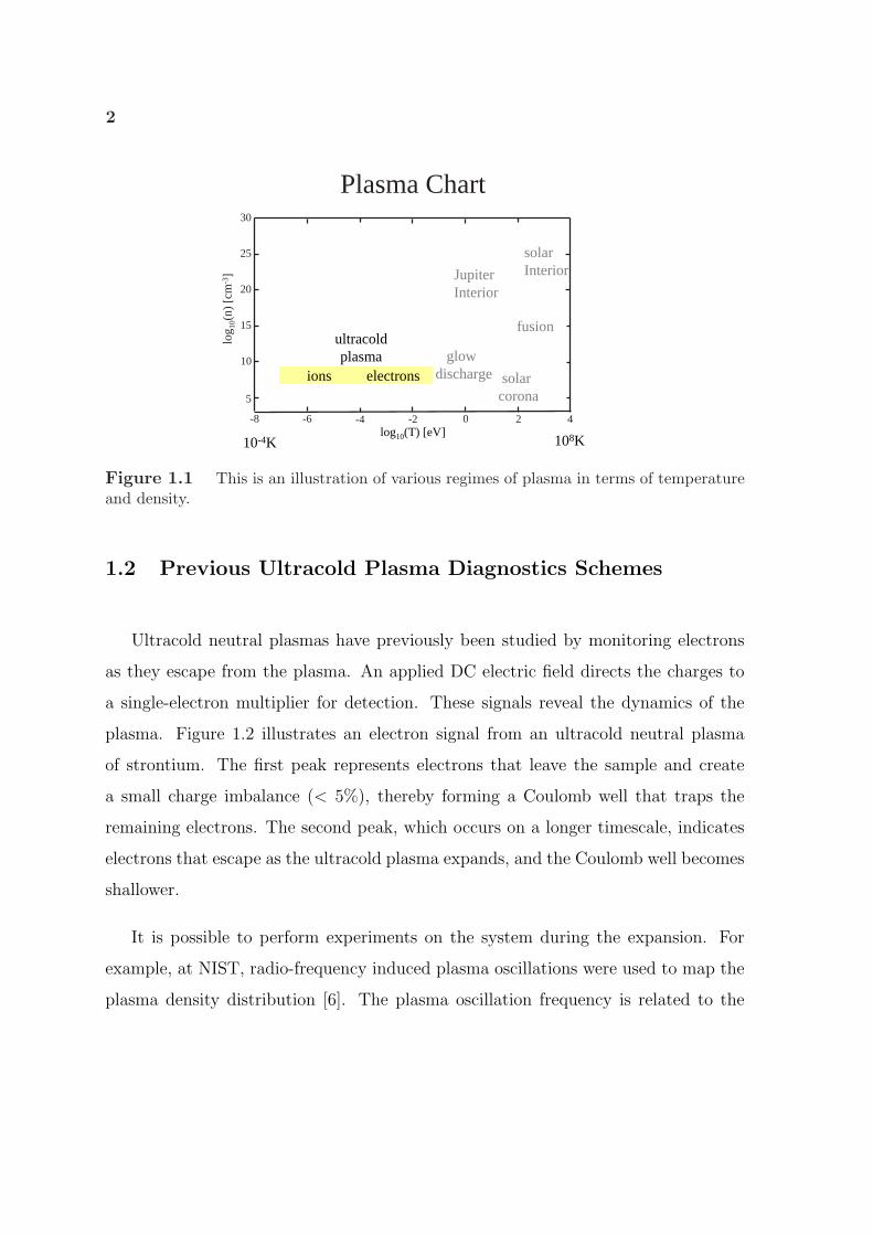
found in the universe (Figure 1.1). Interest in these system stems from the question
of whether plasmas behave differently in this regime.
2
Plasma Chart
5
10
15
20
25
30
-6 -4 -2 0 2 4-8
log 1
0(n)
[cm
-3]
fusion
log10(T) [eV]
ultracoldplasma
ions electrons
JupiterInterior
solarcorona
glowdischarge
solarInterior
10-4K 108K
Figure 1.1 This is an illustration of various regimes of plasma in terms of temperatureand density.
1.2 Previous Ultracold Plasma Diagnostics Schemes
Ultracold neutral plasmas have previously been studied by monitoring electrons
as they escape from the plasma. An applied DC electric field directs the charges to
a single-electron multiplier for detection. These signals reveal the dynamics of the
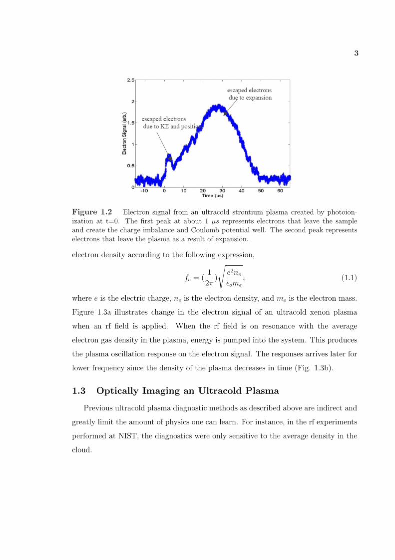
plasma. Figure 1.2 illustrates an electron signal from an ultracold neutral plasma
of strontium. The first peak represents electrons that leave the sample and create
a small charge imbalance (< 5%), thereby forming a Coulomb well that traps the
remaining electrons. The second peak, which occurs on a longer timescale, indicates
electrons that escape as the ultracold plasma expands, and the Coulomb well becomes
shallower.
It is possible to perform experiments on the system during the expansion. For
example, at NIST, radio-frequency induced plasma oscillations were used to map the
plasma density distribution [6]. The plasma oscillation frequency is related to the
3
Figure 1.2 Electron signal from an ultracold strontium plasma created by photoion-ization at t=0. The first peak at about 1 µs represents electrons that leave the sampleand create the charge imbalance and Coulomb potential well. The second peak representselectrons that leave the plasma as a result of expansion.
electron density according to the following expression,
fe = (1
2π)
√e2ne
εome
, (1.1)
where e is the electric charge, ne is the electron density, and me is the electron mass.
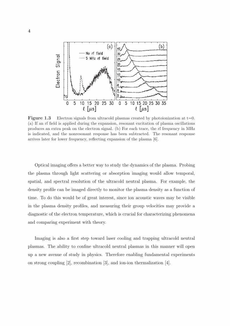
Figure 1.3a illustrates change in the electron signal of an ultracold xenon plasma
when an rf field is applied. When the rf field is on resonance with the average
electron gas density in the plasma, energy is pumped into the system. This produces
the plasma oscillation response on the electron signal. The responses arrives later for
lower frequency since the density of the plasma decreases in time (Fig. 1.3b).
1.3 Optically Imaging an Ultracold Plasma
Previous ultracold plasma diagnostic methods as described above are indirect and
greatly limit the amount of physics one can learn. For instance, in the rf experiments
performed at NIST, the diagnostics were only sensitive to the average density in the
cloud.
4
Figure 1.3 Electron signals from ultracold plasmas created by photoionization at t=0.(a) If an rf field is applied during the expansion, resonant excitation of plasma oscillationsproduces an extra peak on the electron signal. (b) For each trace, the rf frequency in MHzis indicated, and the nonresonant response has been subtracted. The resonant responsearrives later for lower frequency, reflecting expansion of the plasma [6].
Optical imaging offers a better way to study the dynamics of the plasma. Probing
the plasma through light scattering or absorption imaging would allow temporal,
spatial, and spectral resolution of the ultracold neutral plasma. For example, the
density profile can be imaged directly to monitor the plasma density as a function of
time. To do this would be of great interest, since ion acoustic waves may be visible
in the plasma density profiles, and measuring their group velocities may provide a
diagnostic of the electron temperature, which is crucial for characterizing phenomena
and comparing experiment with theory.
Imaging is also a first step toward laser cooling and trapping ultracold neutral
plasmas. The ability to confine ultracold neutral plasmas in this manner will open
up a new avenue of study in physics. Therefore enabling fundamental experiments
on strong coupling [2], recombination [3], and ion-ion thermalization [4].
5
1.4 Outline
This thesis will describe the construction of a blue laser source at 421.7 nm. In
chapter 2 we will discuss second-harmonic generation. Next, in chapter 3 we will
go over the gaussian optics of resonators. In chapter 4 we will describe our optical
resonator, discuss the experimental procedures to produce light at 421.7 nm, and
analyze the performance of our blue laser source. Chapter 5 will cover the feedback
electronics used to stabilize our laser system. Finally, in chapter 6, we will conclude
this thesis with a brief discussion on the limitations of our blue laser source and
display some preliminary imaging results.

Chapter 2
Second Harmonic Generation
This chapter discusses the concepts of Second-Harmonic Generation, and gives a
brief description of the properties of potassium niobate.
2.1 Theory
Nonlinear optical phenomena in the interaction of light with a particular media is
a result of the nonlinear nature of the polarization, which can be written in terms of
the electric field E as:
P = εoχ1E + εoχ2E2 + εoχ3E
3, (2.1)
where χ1 is the linear susceptibility, χ2 is the second-order susceptibility, and χ3 is the
third-order susceptibility. The term χ2 is responsible for second- harmonic generation.
Second-harmonic generation is a nonlinear process in which an electromagnetic
wave with frequency ω is converted into one at frequency 2ω. Consider an electro-
magnetic field with frequency ω1=ω travelling along the z-axis through a crystal with
a non-zero χ2. This interaction of light with the material will create a polarization
wave in the crystal with frequency ω2=2ω. This polarization wave will then produce
radiation at ω2. The power of this radiation is related to the power at ω with beam
area A by the following relation:
Pω2 = [2η3
oω22d
2effL
2
A]P 2
ω1(sin 4kL
24kL
2
)2 = ξnLP 2ω1
(sin 4kL
24kL
2
)2, (2.2)
where
∆k =2ω1(n1 − n2)
c. (2.3)
L is the length of the medium, deff is the nonlinear coefficient of the doubling
crystal, and ηo =377/n1 [7]. The term ξnL is the nonlinear- conversion efficiency. n1
and n2 are the index of refraction at ω1 and ω2 respectively.
7
2.2 Phase Matching
In Eq. 2.2 we can see that second-harmonic power is maximized when 4kL=0.
When this happens, the second harmonic wave and fundamental wave inside of the
material are phase matched. Physically this occurs when nω1=nω2 , which means that
both waves must have the same phase velocities inside the crystal. If the phase veloc-
ities of the two waves are not equivalent, then second harmonic waves generated at
different planes throughout the crystal will destructively interfere with each other, as
described by the sinc function in Eq. 2.2, thereby resulting in low ω1 to ω2 conversion
efficiency.
Usually in materials, nω1 > nω2 , therefore phase matching is not achievable (dis-
persion effect). However, in birefringent materials, materials that posses different
values of indicies of refraction in different directions, the phase matching condition
nω1=nω2 can be satisfied: light with frequency ω1 is polarized along one axis of the
crystal, while light with frequency ω2 is generated along another perpendicular crystal
axis.
2.3 Potassium Niobate
The frequency doubling crystal is required to be sufficiently birefringent to sat-
isfy the phase matching criterion and optically transparent at both the fundamental
and second harmonic wavelengths. It should also have a large non-zero deff . Potas-
sium Niobate (KNbO3) meets these requirements, and it is used in most system for
frequency doubling into the blue-green spectral range. KNbO3 is a biaxial crystal
having principal (symmetric) axes with refractive indicies na 6= nb 6= nc (a, b, and c
are subscripts used by convention to denote the principal axis of the crystal).
In KNbO3 phase matching can be achieved either by changing the angle at which
the fundamental wave propagates with respect to the optical axis of the crystal, or
by tuning the temperature of the crystal (Type I), since the index of refraction is
8
also temperature dependent. For our purpose, temperature-tuned phase matching
is suitable, since KNbO3 can be non-critically temperature-tuned phase matched
for wavelengths from 840-1080 nm, which is a consequence of the strong temper-
ature dependance of the refractive index along the c-axis. In Type I non-critical
temperature-tuned phase matching the input and second harmonic beams are set-up
to propagate along the a-axis of the crystal (a principal axis of the crystal), which
has the advantage of a larger angular acceptance bandwidth and a vanishing walk-off
angle [8]. The polarizations of the two beams are along the b-axis and c-axis respec-
tively. The temperature of the crystal in this type of configuration is adjusted such
that the refraction index experienced by the harmonic wave (polarized along c-axis)
becomes the same as the refraction index experienced by the fundamental wave.
In addition, KNbO3 is optically transparent from 400-3400 nm. It also has a deff
approximately -21 pm/V . This value is a factor of four larger than most doubling
crystals. For instance, LiNbO3 deff is approximately 5.3 pm/V [9],[10].

Chapter 3
844nm Enhancement Optical Resonator
In this chapter the theoretical concepts used when designing an optical resonator
will be discussed. This includes the motivation for the use of an optical resonator for
second harmonic generation, gaussian modes and beams inside an optical resonator,
and the coupling of light from an external source into an optical resonator.
3.1 Motivation
Equation 2.2 illustrates that the second harmonic power depends quadratically on
the fundamental power. Thus, large amounts of fundamental power will result in high
conversion efficiencies. Unfortunately, standard inexpensive continuous wave lasers
do not produce powers that will yield significant conversion from infrared-to-blue.
However, we can enhance the modest powers from commercial lasers with the use of
an optical resonator.
An optical resonator is a set of two or more mirrors configured to allow light to
propagate in a closed path. The enhancement of an optical resonator results from the
effective number of round-trips the light makes along its closed path. For an optical
resonator consisting of two mirrors having reflectivities Ra and Rb, the circulating
power inside the optical resonator is expressed as [14]:
Pc =(1−Ra)Pinput
[1−√
RaRb(1− `− C)]2= bPinput, (3.1)
where Pinput is the input power of the laser, ` is the resonator round-trip parasitic
loss excluding the input mirror transmission Ta and conversion to blue, and b is the
effective number of photon round-trips in the cavity. The term C=ξnLPc is infrared-
to-blue conversion loss (IBCL), which describes the fraction of infrared light loss per
pass to second-harmonic generation, which will be discussed in detail in chapter 4.
10
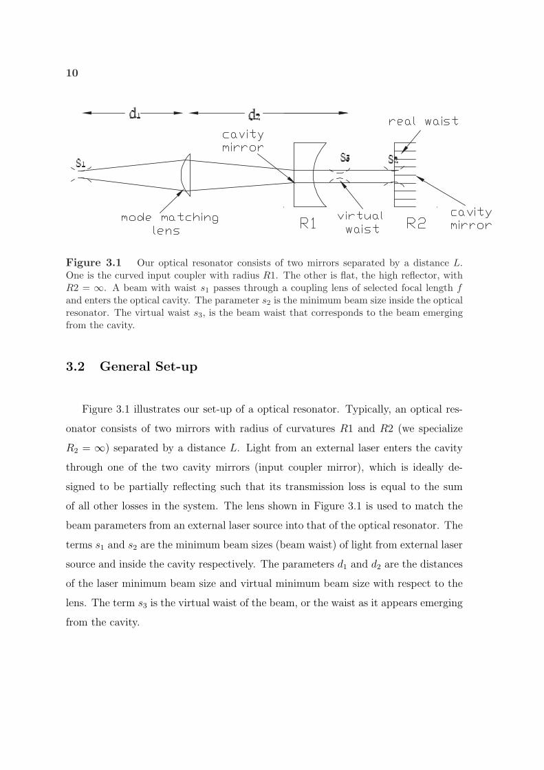
Figure 3.1 Our optical resonator consists of two mirrors separated by a distance L.One is the curved input coupler with radius R1. The other is flat, the high reflector, withR2 = ∞. A beam with waist s1 passes through a coupling lens of selected focal length fand enters the optical cavity. The parameter s2 is the minimum beam size inside the opticalresonator. The virtual waist s3, is the beam waist that corresponds to the beam emergingfrom the cavity.
3.2 General Set-up
Figure 3.1 illustrates our set-up of a optical resonator. Typically, an optical res-
onator consists of two mirrors with radius of curvatures R1 and R2 (we specialize
R2 = ∞) separated by a distance L. Light from an external laser enters the cavity
through one of the two cavity mirrors (input coupler mirror), which is ideally de-
signed to be partially reflecting such that its transmission loss is equal to the sum
of all other losses in the system. The lens shown in Figure 3.1 is used to match the
beam parameters from an external laser source into that of the optical resonator. The
terms s1 and s2 are the minimum beam sizes (beam waist) of light from external laser
source and inside the cavity respectively. The parameters d1 and d2 are the distances
of the laser minimum beam size and virtual minimum beam size with respect to the
lens. The term s3 is the virtual waist of the beam, or the waist as it appears emerging
from the cavity.
11
3.3 Gaussian Modes
Following [11], the electric field component for laser light travelling in the z direc-
tion can be written as
u = ψ(x, y, z) exp(−jkz) (3.2)
where ψ is the transverse electric field pattern of the laser beam. The wave equation
in cylindrical coordinates that describes these modes is the following:
1
r
∂
∂rr∂ψ
∂r− j2kc
∂ψ
∂z= 0, (3.3)
where kc is the vacuum wave vector. There are many solutions to the above equation
having different transverse modes (spatial patterns). The lowest order transverse
mode of equation 3.3 is called the TEM00 or Gaussian mode and is ubiquitous in
laser systems used for atomic physics research. This mode is circular in its transverse
dimension, and has very nice focusing properties. Mathematically, it is expressed as
ψ = exp[−j(P (z) +kr2
2q(z))], (3.4)
where q(z) is the confocal parameter, describing the variation in beam intensity with
distance from the optical axis, and P (z) is the complex phase shift. These two
parameters are defined as the following:
1
q(z)=
1
R(z)− jλ0
πs(z)2, (3.5)
P (z) = (kz − Φ). (3.6)
where s(z) =√
s2o[1 + ( λz
πs2o)2] is the 1/e2 intensity radius or spot size of the gaussian
beam, R(z) = z[1 + (πs2o
λz)2] is the wavefront radius of curvature, and Φ = arctan( λz
πs2o)
represents a phase shift difference between an ideal plane wave and Gaussian beam.
The quantity s0 in the expression for s(z), R(z), and Φ(z) is the beam waist. Following
from equations 3.2 - 3.6, the gaussian beam transverse intensity pattern is written as:
I(x, y, z) =2P
πs(z)2exp[
−2(x2 + y2)
s(z)2], (3.7)
where P is the power of the laser beam.
12
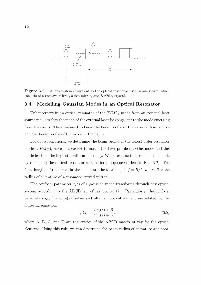
Figure 3.2 A lens system equivalent to the optical resonator used in our set-up, whichconsists of a concave mirror, a flat mirror, and KNbO3 crystal.
3.4 Modelling Gaussian Modes in an Optical Resonator
Enhancement in an optical resonator of the TEM00 mode from an external laser
source requires that the mode of the external laser be congruent to the mode emerging
from the cavity. Thus, we need to know the beam profile of the external laser source
and the beam profile of the mode in the cavity.
For our applications, we determine the beam profile of the lowest-order resonator
mode (TEM00), since it is easiest to match the laser profile into this mode and this
mode leads to the highest nonlinear efficiency. We determine the profile of this mode
by modelling the optical resonator as a periodic sequence of lenses (Fig. 3.2). The
focal lengths of the lenses in the model are the focal length f = R/2, where R is the
radius of curvature of a resonator curved mirror.
The confocal parameter q(z) of a gaussian mode transforms through any optical
system according to the ABCD law of ray optics [12]. Particularly, the confocal
parameters q1(z) and q2(z) before and after an optical element are related by the
following equation:
q2(z) =Aq1(z) + B
Cq1(z) + D, (3.8)
where A, B, C, and D are the entries of the ABCD matrix or ray for the optical
elements. Using this rule, we can determine the beam radius of curvature and spot-
13
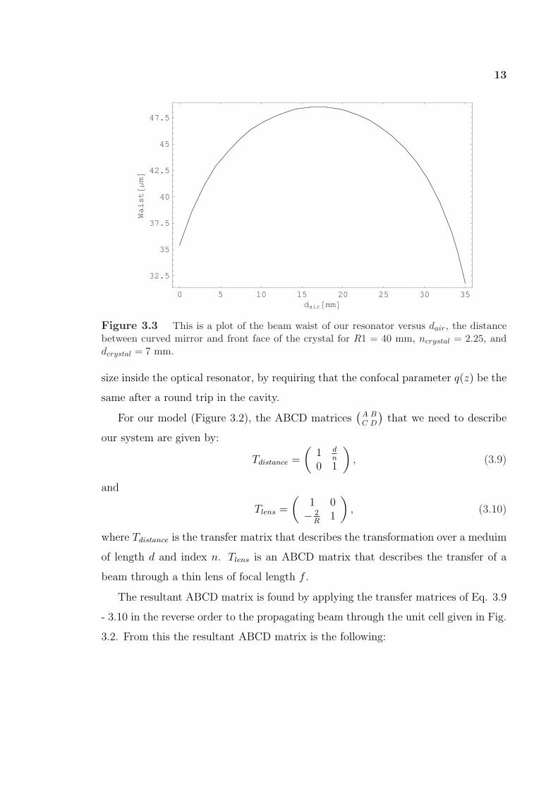
0 5 10 15 20 25 30 35dair@mmD
32.5
35
37.5
40
42.5
45
47.5
Waist@ΜmD
Figure 3.3 This is a plot of the beam waist of our resonator versus dair, the distancebetween curved mirror and front face of the crystal for R1 = 40 mm, ncrystal = 2.25, anddcrystal = 7 mm.
size inside the optical resonator, by requiring that the confocal parameter q(z) be the
same after a round trip in the cavity.
For our model (Figure 3.2), the ABCD matrices(
AC
BD
)that we need to describe
our system are given by:
Tdistance =
(1 d
n
0 1
), (3.9)
and
Tlens =
(1 0− 2
R1
), (3.10)
where Tdistance is the transfer matrix that describes the transformation over a meduim
of length d and index n. Tlens is an ABCD matrix that describes the transfer of a
beam through a thin lens of focal length f .
The resultant ABCD matrix is found by applying the transfer matrices of Eq. 3.9
- 3.10 in the reverse order to the propagating beam through the unit cell given in Fig.
3.2. From this the resultant ABCD matrix is the following:
14
(A BC D
)=
(1
dcrystal
ncrystal
0 1
)(1 dair
nair
0 1
)(1 0−2R1
1
) (1 dair
nair
0 1
) (1
dcrystal
ncrystal
0 1
)
=
1− 2(
dairnair
+dcrystalncrystal
)
R1
2(dcrystalnair+dairncrystal)(dcrystalnair+ncrystal(dair−nairR1))
n2airn2
crystalR1
− 2R1
1− 2dair
nairR1− 2dcrystal
ncrystalR1
(3.11)
where dcrystal is the crystal length, nair and ncrystal is the air and crystal index of
refraction respectively, and dair is the distance from the input coupler to front-face of
crystal.
By setting q1(z) = q2(z) in Eq. 3.8 and using the ABCD elements of Eq. 3.11 we
obtain the following expression for the resonator beam waist
s22 =
2λB
π√
4− (A + D)2, (3.12)
and it is by symmetry located at the flat mirror (The beam waist is at the location
that corresponds to R(z) = ∞.). Figure 3.3 is a plot of Eq. 3.12 (resonator beam
waist) as a function of dair, the distance between the curved mirror and front face of
the crystal.
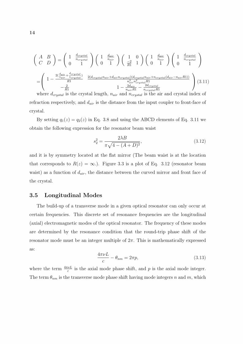
3.5 Longitudinal Modes
The build-up of a transverse mode in a given optical resonator can only occur at
certain frequencies. This discrete set of resonance frequencies are the longitudinal
(axial) electromagnetic modes of the optical resonator. The frequency of these modes
are determined by the resonance condition that the round-trip phase shift of the
resonator mode must be an integer multiple of 2π. This is mathematically expressed
as:4πνL
c− θnm = 2πp, (3.13)
where the term 4πνLc
is the axial mode phase shift, and p is the axial mode integer.
The term θnm is the transverse mode phase shift having mode integers n and m, which
15
varies for different modes. The resonance frequencies obtained from Eq. 3.13 are the
following:
νpnm = pc
2L+
θnmc
4πL(3.14)
where L is the cavity length and c is the speed of light in vacuum. In Eq. 3.14
c2L
is the free-spectral range (FSR) of the optical resonator, which is the frequency
separation between adjacent TEM00 longitudinal modes in Hz. The transverse mode
spectrum is described by the term θnmc4πL
and will be illustrated and briefly discussed
in Chapter 4.
3.6 Resonator Losses
The frequency criterion for optical waves to exist inside a resonator is relaxed,
when the resonator has losses [13], for example, when the mirrors are not perfect
reflectors. The losses of a cavity are describe by the finesse z, which is expressed in
terms of the overall losses in the system α as:
z =π exp[−α]D
1− exp[−2α]D' 2π
αD, (3.15)
where α is given by
αD = ` + C + ln1
RaRb
, (3.16)
where ` is the round-trip parasitic loss and C is the infrared blue conversion loss. The
term ln 1RaRb
is losses due to mirror reflectivities. For Rb ' 1 Eq. 3.15 reduces to the
following:
z ' 2π
` + C + Ta
, (3.17)
where Ta' 1−Ra is transmission of the input coupler mirror. In the presence of these
the modes are no longer discrete sharp peaks as a function of frequency, but have a
spectral full-width-half-maximum (FWHM) Γ given by:
Γ =FSR
z. (3.18)
Chapter 4
Experimental Details
This chapter discusses the experimental layout, the optical resonator design, and
the experimental procedure used to convert light at 844 nm to 422 nm.
4.1 Experimental Apparatus
The experimental set-up used to produce light at 422 nm is displayed in Figure
4.1 and Figure 4.2. In Fig. 4.1, p-polarized light is emitted from a Toptica single
frequency high powered tunable diode laser and coupled into a optical fiber. The
output light from the fiber ranges in power from 10-120 mW and has a virtual beam
waist of 82.9 µm located approximately 12 cm behind the output fiber head.
The light from the fiber passes through an f = 200 mm focal length lens (for
mode matching), and a dichroic mirror, before passing into the optical resonator.
The optical resonator is semi-monolithic, consisting of an input coupling mirror and
a KNbO3 crystal. The input coupler mirror, which is mounted on a piezo-electric
transducer (PZT) to adjust the cavity length, has radius of curvature of 40 mm,
transmits 5% at 844 nm and 90% at 422 nm, and serves as a output coupler for the
blue. The KNbO3 crystal is 7 mm in length and is ”a-cut”, which means the principal
axes of the crystal is oriented such that the fundamental light propagates along the
crystal’s a-axis with its polarization along its b-axis. The end faces of the crystal are
flat. The front interface is anti-reflection coated for the 844 nm and 422 nm light.
The crystal back face serves as the mirror and it is dielectrically coated as a high
reflector with reflectivity of .999 for light at 844 nm and 422 nm (Fig. 4.3 ).
The KNbO3 crystal is wrapped in indium foiled and resides inside an aluminum
enclosure (not shown). This enclosure sets on top of two cascaded Thorlabs 3-6
amp thermo-electric coolers for active control of the crystal temperature. In turn,

17
Figure 4.1 Schematic of the experimental configuration (not to scale). HR, high reflec-tor, HT, high transmission.
Figure 4.2 The crystal-mirror arrangement used in our system.
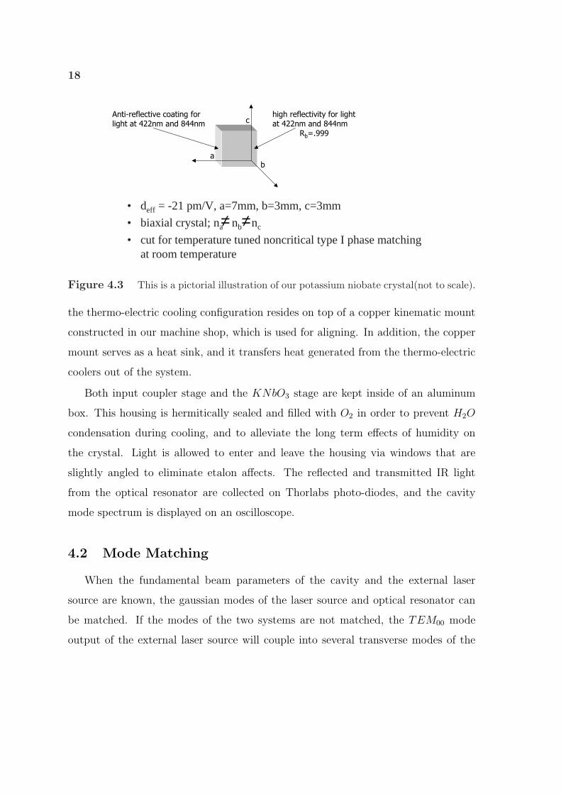
18 Potassium Niobate Crystal (KNBO3)
• deff = -21 pm/V, a=7mm, b=3mm, c=3mm
• biaxial crystal; na nb nc
• cut for temperature tuned noncritical type I phase matching at room temperature
high reflectivity for light at 422nm and 844nm
Rb=.999
Anti-reflective coating forlight at 422nm and 844nm
≠ ≠
c
ba
Figure 4.3 This is a pictorial illustration of our potassium niobate crystal(not to scale).
the thermo-electric cooling configuration resides on top of a copper kinematic mount
constructed in our machine shop, which is used for aligning. In addition, the copper
mount serves as a heat sink, and it transfers heat generated from the thermo-electric
coolers out of the system.
Both input coupler stage and the KNbO3 stage are kept inside of an aluminum
box. This housing is hermitically sealed and filled with O2 in order to prevent H2O
condensation during cooling, and to alleviate the long term effects of humidity on
the crystal. Light is allowed to enter and leave the housing via windows that are
slightly angled to eliminate etalon affects. The reflected and transmitted IR light
from the optical resonator are collected on Thorlabs photo-diodes, and the cavity
mode spectrum is displayed on an oscilloscope.
4.2 Mode Matching
When the fundamental beam parameters of the cavity and the external laser
source are known, the gaussian modes of the laser source and optical resonator can
be matched. If the modes of the two systems are not matched, the TEM00 mode
output of the external laser source will couple into several transverse modes of the
19
cavity, which will limit the enhancement of the external laser’s fundamental mode.
Thus, to prevent the excitement of additional resonator modes, a lens is used to
transform the TEM00 from the laser into that of the cavity. This phenomena is
known as mode matching.
In general, to mode match, only the sizes and positions of the beam waists of
both systems need to be known. Once that information is at hand, the problem is
to determine the focal length and the distances from each waist to the lens that are
needed to match the two systems, as illustrated in Figure 3.1.
In practice, the input-coupler mirror of the optical resonator is a fused silica
substrate. This substrate acts as a plano-concave lens of focal length −2Rmirror,
where Rmirror is the radius of curvature of the input coupler. This effect, in turn,
causes the waist size and location for the beam that emerges from the cavity to be
different from that of the resonator. Therefore, in order to properly mode match we
must take into consideration this lens action, and determine the size, s3, and location
of this virtual beam waist [12].
We determined the size of the virtual beam waist using the following equation
[15]:
s3 =fλ
πS[(1− flens
R)2 + (
λflens
πS2)2]−
12 , (4.1)
where S and R are the beam spot size and radius of curvature of the resonator mode
at the location of the input coupler. The term flens is the focal length of the input
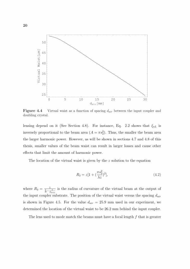
coupler substrate. Figure 4.4 is a plot of the virtual waist of our system as a function
of spacing dair between the input coupler and doubling crystal. For our experimental
configuration, the chosen distance between the front-face of the doubler crystal and
the input coupler mirror (dair = 25.9 mm) results in a virtual waist s3 of 29.0 µm
and a resonator beam waist s2 of 45.9 µm.
The size of the resonator beam waist is critical in frequency doubling experiments,
since the harmonic power, losses (BLIRA), and other mechanisms such as thermal
20
0 5 10 15 20 25 30dair@mmD
25
30
35
40
45
50VirtualWaist@ΜmD
Figure 4.4 Virtual waist as a function of spacing dair between the input coupler anddoubling crystal.
lensing depend on it (See Section 4.8). For instance, Eq. 2.2 shows that ξnL is
inversely proportional to the beam area (A = πs22). Thus, the smaller the beam area
the larger harmonic power. However, as will be shown in sections 4.7 and 4.8 of this
thesis, smaller values of the beam waist can result in larger losses and cause other
effects that limit the amount of harmonic power.
The location of the virtual waist is given by the z solution to the equation
R3 = z[1 + (πs2
3
λz)2], (4.2)
where R3 = 11R− 1
flens
is the radius of curvature of the virtual beam at the output of
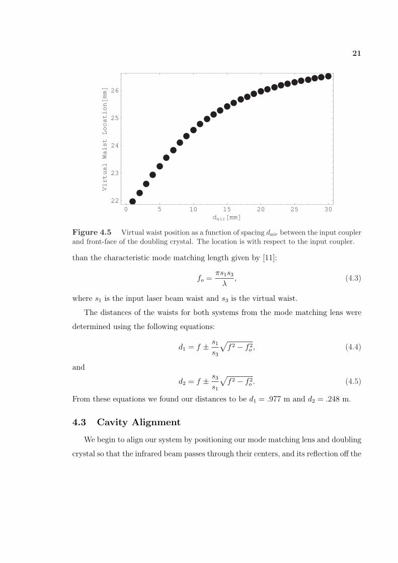
the input coupler substrate. The position of the virtual waist versus the spacing dair
is shown in Figure 4.5. For the value dair = 25.9 mm used in our experiment, we
determined the location of the virtual waist to be 26.2 mm behind the input coupler.
The lens used to mode match the beams must have a focal length f that is greater
21
0 5 10 15 20 25 30dair@mmD
22
23
24
25
26
Virtual
Waist
Location@mmD
Figure 4.5 Virtual waist position as a function of spacing dair between the input couplerand front-face of the doubling crystal. The location is with respect to the input coupler.
than the characteristic mode matching length given by [11]:
fo =πs1s3
λ, (4.3)
where s1 is the input laser beam waist and s3 is the virtual waist.
The distances of the waists for both systems from the mode matching lens were
determined using the following equations:
d1 = f ± s1
s3
√f 2 − f 2
o , (4.4)
and
d2 = f ± s3
s1
√f 2 − f 2
o . (4.5)
From these equations we found our distances to be d1 = .977 m and d2 = .248 m.
4.3 Cavity Alignment
We begin to align our system by positioning our mode matching lens and doubling
crystal so that the infrared beam passes through their centers, and its reflection off the
22
back cavity mirror overlaps with the incident beam. Then we place the input coupler
mirror, which is attached to a PZT and mounted on to an optical mount, into the
system and adjusted it such that the reflection beam from the input coupler overlaps
with the input beam of the laser. Next, we modulated the PZT, and transmission of
the TEM00 cavity mode along with many other higher order cavity modes through
the back-face of the crystal were visible on the output from the photo-diode. Finally,
we adjust the input coupler mirror, the doubler crystal, and mirrors M1 and M2 in
Fig. 4.1 to couple most of the power into the TEM00 mode.
4.4 Cavity Modes
In our experimental configuration we use our optical resonator as a scanning in-
terferometer in order to monitor the mode spectra. As we scan the length of our
cavity, when the laser sequentially comes into resonance with a cavity longitudinal
mode, light enters the cavity, and excites the cavity modes. Mathematically, the
laser-cavity resonance condition for two adjacent modes is expressed as:
fl =pc
2L=
(p + 1)c
2(L + ∆L)(4.6)
where fl is the laser frequency, p is the axial mode number, and ∆L = α∆V is the
change in cavity length (corresponding to a FSR) in terms of a change in PZT voltage
∆V . The term α is the PZT voltage to length proportionality constant.
Figure 4.6 is the mode spectrum of our optical resonator. The large sharp peaks, p
and (p+1), are the TEM00 of the cavity, which are separated by 1FSR (∆V'100V).
The next taller peaks is are higher-order transverse modes, which are shifted from
the fundamental modes by 14
FSR. From the figure we estimated that more than 90%
of the external laser power is coupled into the gaussian mode of the resonator.
We measured the separation of the p and (p + 1) cavity modes by turning off
the PZT scan, and scanning our 844 nm laser frequency. Now, we scan our laser
frequency such that it will sequentially come into resonance with the cavity. While

23
0 1 2 3 4 5 6 7 80
0.1
0.2
0.3
0.4
0.5
0.6
0.7
0.8
0.9
1Transmission Modes
Frequency[GHz]
Sig
nal[a
rbitr
ary
units
]
p (p+1)
Figure 4.6 Mode spectrum of 844 nm IR enhancement cavity, with fit function.
24
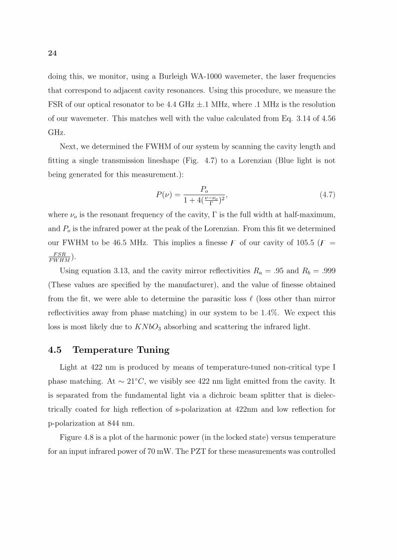
doing this, we monitor, using a Burleigh WA-1000 wavemeter, the laser frequencies
that correspond to adjacent cavity resonances. Using this procedure, we measure the
FSR of our optical resonator to be 4.4 GHz ±.1 MHz, where .1 MHz is the resolution
of our wavemeter. This matches well with the value calculated from Eq. 3.14 of 4.56
GHz.
Next, we determined the FWHM of our system by scanning the cavity length and
fitting a single transmission lineshape (Fig. 4.7) to a Lorenzian (Blue light is not
being generated for this measurement.):
P (ν) =Po
1 + 4(ν−νo
Γ)2
, (4.7)
where νo is the resonant frequency of the cavity, Γ is the full width at half-maximum,
and Po is the infrared power at the peak of the Lorenzian. From this fit we determined
our FWHM to be 46.5 MHz. This implies a finesse z of our cavity of 105.5 (z =
FSRFWHM
).
Using equation 3.13, and the cavity mirror reflectivities Ra = .95 and Rb = .999
(These values are specified by the manufacturer), and the value of finesse obtained
from the fit, we were able to determine the parasitic loss ` (loss other than mirror
reflectivities away from phase matching) in our system to be 1.4%. We expect this
loss is most likely due to KNbO3 absorbing and scattering the infrared light.
4.5 Temperature Tuning
Light at 422 nm is produced by means of temperature-tuned non-critical type I
phase matching. At ∼ 21◦C, we visibly see 422 nm light emitted from the cavity. It
is separated from the fundamental light via a dichroic beam splitter that is dielec-
trically coated for high reflection of s-polarization at 422nm and low reflection for
p-polarization at 844 nm.
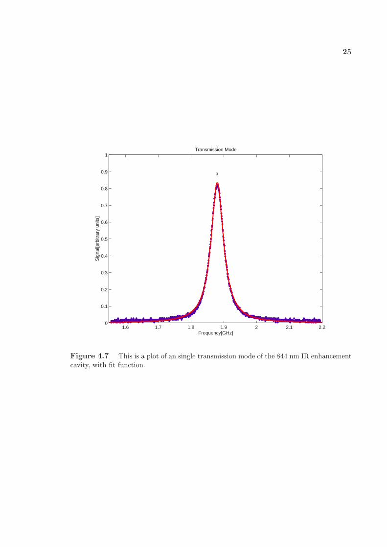
Figure 4.8 is a plot of the harmonic power (in the locked state) versus temperature
for an input infrared power of 70 mW. The PZT for these measurements was controlled
25
1.6 1.7 1.8 1.9 2 2.1 2.20
0.1
0.2
0.3
0.4
0.5
0.6
0.7
0.8
0.9
1
Frequency[GHz]
Sig
nal[a
rbitr
ary
units
]
Transmission Mode
p
Figure 4.7 This is a plot of an single transmission mode of the 844 nm IR enhancementcavity, with fit function.
26
−21.65 −21.6 −21.55 −21.5 −21.45 −21.4 −21.35 −21.3 −21.252
4
6
8
10
12
14Phasematching Temperature Profile
Temperature (C)
422n
m P
ower
(m
W)
Figure 4.8 This is the temperature tuning curve for our blue laser source having aninput infrared power of 70 mW.

27
0 20 40 60 80 100 120−21.9
−21.8
−21.7
−21.6
−21.5
−21.4
−21.3
−21.2Phase Matching Temperature Curve
Tem
pera
ture
(C
)
Input IR Power (mW)
Figure 4.9 The optimal phase-matching temperature increases with larger incidentpower. This response is due to the heating of the crystal as a result of more circulatingpower in the cavity.
such that its length always corresponds to maximal build-up inside the cavity. In this
locked state of the cavity, for 70 mW of fundamental power, the maximum blue power
occurred at a temperature of −21.47◦C. This is close to the value of −20◦C estimated
from the graph given in [8]. We took the temperature bandwidth for phase matching
in our configuration as the FWHM of this peak, which is ∼ .3◦C. Using Eq. 4.6 [9]
∆T =.443λ1
L‖∂nb
∂T− ∂nc
∂T‖ , (4.8)
where ∂nb
∂T= −3.3 × 10⁻⁵ and ∂nc
∂T= 1.3 × 10⁻⁴ are the thermo-optic coefficients
of KNbO3 and λ1 is the fundamental wavelength. We calculated the value of the
temperature bandwidth to be .324◦C. This value agrees well with our measurement.
Figure 4.9 is a plot of the phase-matching temperature vs. input fundamental
28
0 20 40 60 80 100Mode-matched Fundamental Power@mWD
0
20
40
60
80SecondHarmonicPower@mWD
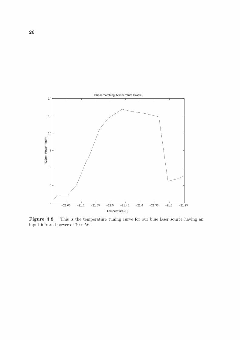
Figure 4.10 Generated second-harmonic power as a function of the mode-matchedfundamental power. The solid, long-dashed, and short-dashed curves are obtained fromtheory. Filled circles are data.
power. This figure shows the decrease in phase-matching temperature with increase
in infrared power. This trend is due to absorption, since as the fundamental power
increases more infrared power and blue power is absorbed by the crystal, thereby
causing it to heat-up. Thus, in order to phase match the crystal with the additional
heat, the temperature of the housing must be decreased to lower values.
4.6 Frequency Doubling
Figure 4.10 is a plot of the harmonic power at 422 nm as a function of the fun-
damental mode-matched power. The filled circles represent the measurements of the
second-harmonic power corrected for transmission losses from the output of the crys-
tal to the blue detector. For a maximum fundamental power of 110 mW out of our
fiber, of which we estimate 83% is optimally coupled into the fundamental mode,
we get a peak second-harmonic power (locked) of 22.6 mW in a single longitudinal
mode. After a series of optical elements, i.e., input coupler mirror, dichroic mirrors,
29
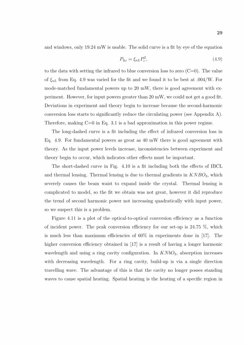
and windows, only 19.24 mW is usable. The solid curve is a fit by eye of the equation
P2ω = ξnLP 2c , (4.9)
to the data with setting the infrared to blue conversion loss to zero (C=0). The value
of ξnL from Eq. 4.9 was varied for the fit and we found it to be best at .004/W. For
mode-matched fundamental powers up to 20 mW, there is good agreement with ex-
periment. However, for input powers greater than 20 mW, we could not get a good fit.
Deviations in experiment and theory begin to increase because the second-harmonic
conversion loss starts to significantly reduce the circulating power (see Appendix A).
Therefore, making C=0 in Eq. 3.1 is a bad approximation in this power regime.
The long-dashed curve is a fit including the effect of infrared conversion loss in
Eq. 4.9. For fundamental powers as great as 40 mW there is good agreement with
theory. As the input power levels increase, inconsistencies between experiment and
theory begin to occur, which indicates other effects must be important.
The short-dashed curve in Fig. 4.10 is a fit including both the effects of IBCL
and thermal lensing. Thermal lensing is due to thermal gradients in KNBO3, which
severely causes the beam waist to expand inside the crystal. Thermal lensing is
complicated to model, so the fit we obtain was not great, however it did reproduce
the trend of second harmonic power not increasing quadratically with input power,
so we suspect this is a problem.
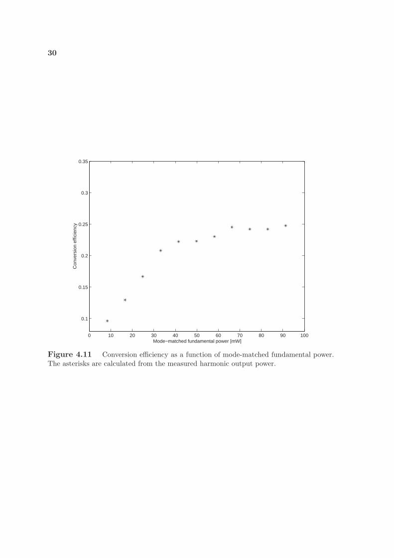
Figure 4.11 is a plot of the optical-to-optical conversion efficiency as a function
of incident power. The peak conversion efficiency for our set-up is 24.75 %, which
is much less than maximum efficiencies of 60% in experiments done in [17]. The
higher conversion efficiency obtained in [17] is a result of having a longer harmonic
wavelength and using a ring cavity configuration. In KNbO3, absorption increases
with decreasing wavelength. For a ring cavity, build-up is via a single direction
travelling wave. The advantage of this is that the cavity no longer posses standing
waves to cause spatial heating. Spatial heating is the heating of a specific region in
30
0 10 20 30 40 50 60 70 80 90 100
0.1
0.15
0.2
0.25
0.3
0.35
Mode−matched fundamental power [mW]
Con
vers
ion
effic
ienc
y
Figure 4.11 Conversion efficiency as a function of mode-matched fundamental power.The asterisks are calculated from the measured harmonic output power.
31
4.6 4.8 5 5.20
0.5
1
1.5
2
2.5
a)
Frequency [GHz]
Sig
nal [
arb.
uni
ts]
3 3.2 3.4 3.6 3.8 40
0.5
1
1.5
2
2.5
b)
Frequency [GHz]
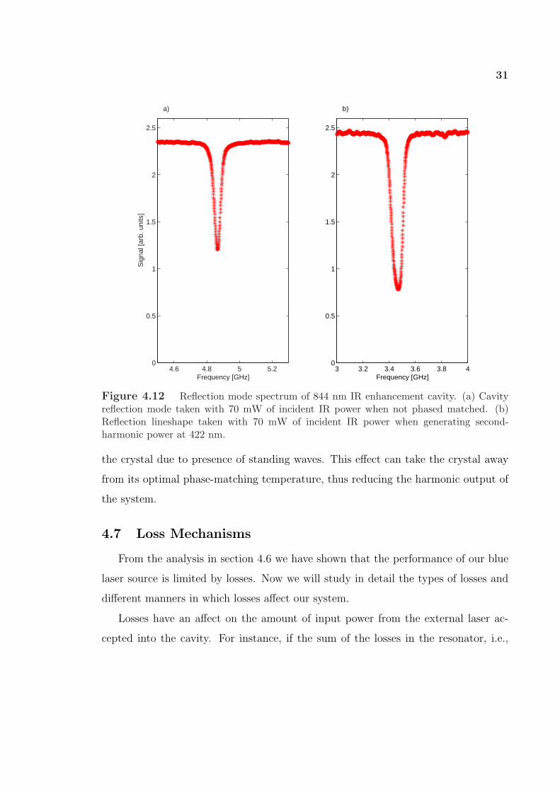
Figure 4.12 Reflection mode spectrum of 844 nm IR enhancement cavity. (a) Cavityreflection mode taken with 70 mW of incident IR power when not phased matched. (b)Reflection lineshape taken with 70 mW of incident IR power when generating second-harmonic power at 422 nm.
the crystal due to presence of standing waves. This effect can take the crystal away
from its optimal phase-matching temperature, thus reducing the harmonic output of
the system.
4.7 Loss Mechanisms
From the analysis in section 4.6 we have shown that the performance of our blue
laser source is limited by losses. Now we will study in detail the types of losses and
different manners in which losses affect our system.
Losses have an affect on the amount of input power from the external laser ac-
cepted into the cavity. For instance, if the sum of the losses in the resonator, i.e.,
32
scattering, absorption, and infrared-to-blue conversion loss does not equal the trans-
mission loss of the input coupler, then a fraction of the input light will reflect from the
cavity. If the sum of the cavity losses equals to the input mirror transmission, then
no light reflects from the cavity, and the optical resonator is said to be impedance
matched [17]. Figure 4.12 is a study of impedance matching for our system.
Figure 4.12a shows the reflected signal from the input coupler mirror, when the
crystal is far away from its phase-matching temperature. The only loss present under
this condition is the parasitic loss, which has a value of 1.4%. For this case, 47.5% of
the incident power is reflected from the cavity. However, in Fig. 4.12 b, which is the
reflected signal from the cavity when the crystal is at phase-matching temperature,
only 22.1% of the power is reflected. This percent change in reflected power is due
to an increase in the losses of our system as we generate 422 nm light. Since, as we
create blue light, the losses in the cavity increase, bringing our system closer to its
impedance matched state. This value is reasonable since the sum of the losses we
account for in our system i.e. parasitic loss, BLIRA, and infrared-to-blue conversion
loss total to 2.5%, which is less than the input mirror transmission of 5%.
We deduced from Fig. 4.12b that the intra-cavity losses increase when generating
blue light. The two loss mechanisms that influence our system in the phase-matching
state is infrared-to-blue conversion loss and BLIRA. BLIRA is a phenomenon where
KNbO3 absorbs infrared light when it is illuminated with blue light.
The infrared-to-blue conversion loss per pass is given by following expression [21]:
C = ξnLPc(Pinput), (4.10)
where Pc is function of Pinput, the mode-matched fundamental power in the cavity.
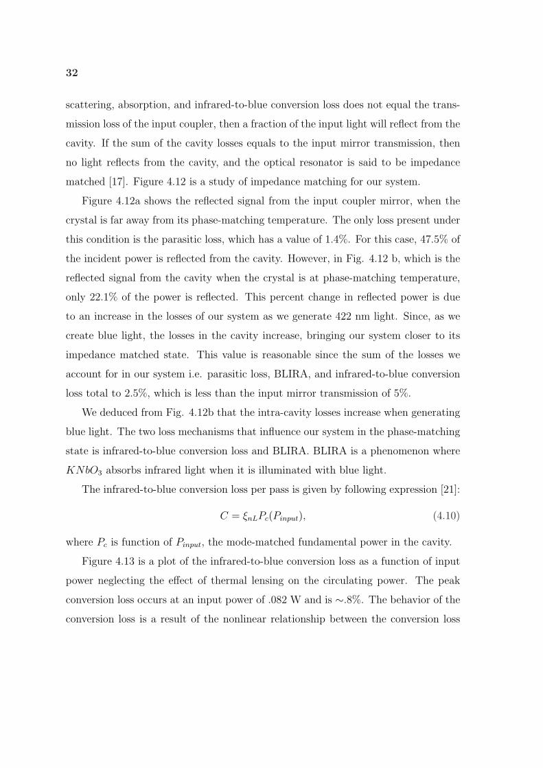
Figure 4.13 is a plot of the infrared-to-blue conversion loss as a function of input
power neglecting the effect of thermal lensing on the circulating power. The peak
conversion loss occurs at an input power of .082 W and is ∼.8%. The behavior of the
conversion loss is a result of the nonlinear relationship between the conversion loss

33
0 20 40 60 80 100Mode-matched Fundamental Power@mWD
0
0.002
0.004
0.006
0.008
Conversion
loss
Figure 4.13 The infrared-to-blue conversion loss as a function of input mode matchedfundamental power in the cavity
and circulating power. For Pinput < .06 W the circulating power is approximately
the enhancement factor, (1−Ra)
[1−√
RaRb(1−`+C)]2, which is essentially a constant value in
this regime, multiplied by the input power. Therefore, the conversion loss increases
linearly with Pinput. However, as the input power exceeds .06 W the conversion
loss increase becomes less with increasing Pinput until it reaches its maximum value.
Afterward, the conversion loss begins to significantly affect the enhancement factor,
and the conversion loss starts to decrease with input power.
Following the expression for the absorbed power density and heat equation given
in [21], we derived an expression for the fraction of power loss due to BLIRA, which
is expressed as:
PBLIRA =
∫
V
24PbPcirδ
π2a4L2exp(
−6r2
a2)z2 dV. (4.11)
The integrand in equation 4.11 is the IR power density absorbed due to BLIRA,
where Pcir and Pb are the circulating and harmonic power. The variables a and L are
the beam waist and crystal length, δ is the BLIRA absorption coefficient, and r is the

34
width of the crystal. We can approximate the crystal as a cylinder, since the beam
area is much less than the square cross section of the crystal. Thus, integration can
be done in cylindrical coordinates.
By integrating over a cylindrical volume we obtained the fraction of infrared power
absorbed due to BLIRA. Thus, for our crystal dimensions L = 7 mm, r = 1.5
mm, and using the value of δ obtained in [22], for a maximum Pcir = 3.5 W and
Pb = 22.6 mW, we determined our peak absorption fraction due to BLIRA to be .5%.
This value is two times smaller than the value obtained in the experiment done in
[17], which achieved a peak conversion efficiency 60%. This comparison along with
the information obtained from fits in Fig. 4.13 suggests to us that BLIRA is not
a significant limiting mechanism in our system. However, it does further support
thermal lensing, since it implies that up to 20 mW of power is being absorbed by
the crystal on axis, which would lead to development of thermal gradients inside the
crystal, thereby causing it to behave as a lens.
4.8 Thermal Effects
Thermal effects can be very harmful to doubling efficiency. For instance, the
absorbed light can cause transverse thermal gradients to arise inside the crystal.
These gradients, in turn, give rise to a spatially dependent index of refraction n(r),
which produces a lens action called thermal lensing [23]. This effect modifies the
beam waist within the crystal, which causes ξnL to decrease. Also, it reduces mode
matching, mode quality, and affects the phase matching of the system.
We evaluated the effect of thermal lensing on our cavity beam waist using the
ABCD matrix formulism. We approximated the transverse temperature distribution
difference T (r) to be quadratic, using the following approximation for T (r) given in
[23],
∆T (r) = ∆T (0)(1− αr2), (4.12)
35
0 20 40 60 80 100Mode-matched Fundamental Power@mWD
50
55
60
65
70
Waist@ΜmD
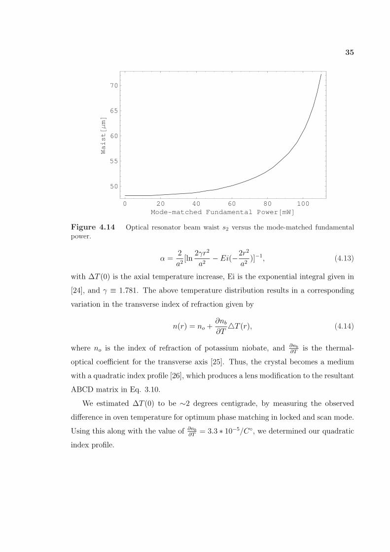
Figure 4.14 Optical resonator beam waist s2 versus the mode-matched fundamentalpower.
α =2
a2[ln
2γr2
a2− Ei(−2r2
a2)]−1, (4.13)
with ∆T (0) is the axial temperature increase, Ei is the exponential integral given in
[24], and γ ≡ 1.781. The above temperature distribution results in a corresponding
variation in the transverse index of refraction given by
n(r) = no +∂nb
∂T4T (r), (4.14)
where no is the index of refraction of potassium niobate, and ∂nb
∂Tis the thermal-
optical coefficient for the transverse axis [25]. Thus, the crystal becomes a medium
with a quadratic index profile [26], which produces a lens modification to the resultant
ABCD matrix in Eq. 3.10.
We estimated ∆T (0) to be ∼2 degrees centigrade, by measuring the observed
difference in oven temperature for optimum phase matching in locked and scan mode.
Using this along with the value of ∂nb
∂T= 3.3 ∗ 10−5/C◦, we determined our quadratic
index profile.
36
Figure 4.14 is a plot of the resonator beam waist incorporating the effect of thermal
lensing into the resonator system. In this figure we illustrate the dependence of our
resonator beam waist s2 in the center of the crystal (r = 0) as function of input
fundamental power. For input powers less than .075 W, changes to the resonator
beam waist with input power are insignificant in the system. However, at higher
input powers, the beam waist begins to increase dramatically in size. This increase
beam waist size reduces ξnL, and therefore the amount of infrared power absorbed or
harmonic power produced.
Comparison of Fig. 4.10 to Fig. 4.14 shows that deviations from the thin-dashed
curve (no thermal lensing) and the thicker dashed curve (thermal lensing) of Fig. 4.10
occur at similar power levels to those in which the resonator beam waist significantly
changes from its original size in Fig. 4.14.
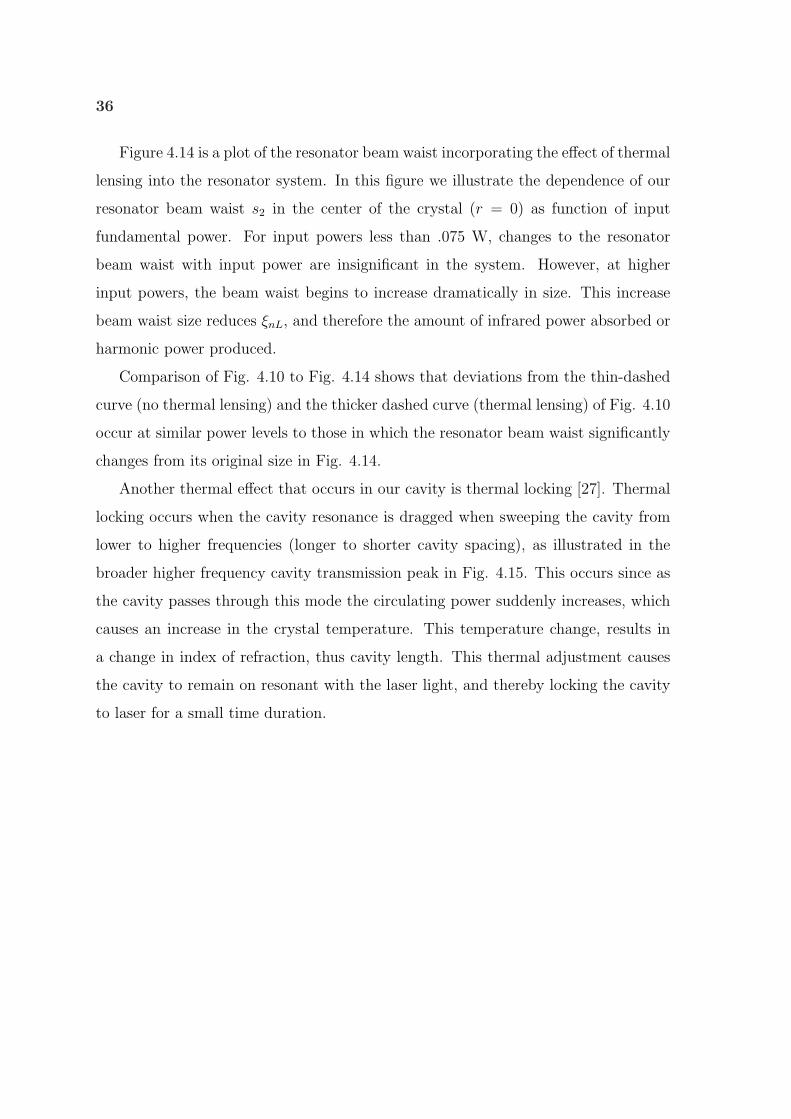
Another thermal effect that occurs in our cavity is thermal locking [27]. Thermal
locking occurs when the cavity resonance is dragged when sweeping the cavity from
lower to higher frequencies (longer to shorter cavity spacing), as illustrated in the
broader higher frequency cavity transmission peak in Fig. 4.15. This occurs since as
the cavity passes through this mode the circulating power suddenly increases, which
causes an increase in the crystal temperature. This temperature change, results in
a change in index of refraction, thus cavity length. This thermal adjustment causes
the cavity to remain on resonant with the laser light, and thereby locking the cavity
to laser for a small time duration.
37
0.05 0.06 0.07 0.08 0.09 0.1 0.11 0.12 0.13 0.14 0.150
2
4
6
8
10
12
14Thermal Locking
Time [s]
Sco
pe T
race
[V]
Transmisson Modes
PZT Ramp
Figure 4.15 A oscilloscope trace illustrating thermal-self-locking. The apparent broad-ening of the line-shape to the right is a result of the resonance being dragged as the cavityis scanned.
Chapter 5
Feedback Electronics
An optical resonator is prone to external perturbations from the environment.
For example, acoustical vibrations from nearby mechanical devices and thermal ex-
pansions and contractions due to temperature fluctuations can prevent our blue laser
source from having a stable intensity output. However, by implementing feedback
electronics we can achieve the desired state for our laser system.
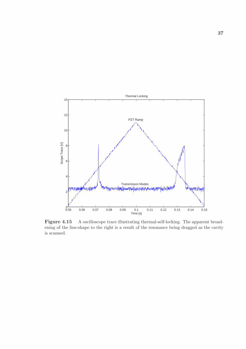
Figure 5.1 is a diagram of the feedback network for our optical resonator. The
network consists of four key elements: 1) The laser, including the input control of its
frequency. This portion changes control voltage into laser frequency. 2) Cavity and
RF electronics, which transform the laser frequency into an error signal. 3) Locking
Electronics, the heart of which is an integrator, which changes volts of error signal
into volts of control. 4) Summing junction, it is used for purposes of feedback into the
laser system [32]. Overall, the loop diagram of Fig. 5.1 controls the laser frequency
to lock the laser to the peak of the transmission mode, such that build-up is always
maximal inside the cavity.
5.1 Error Signal
In our feedback control network, whether or not the laser is at a frequency that
corresponds to maximal of transmission is indicated by the error signal. For our
Figure 5.1 Diagram of feedback network.

39
Figure 5.2 Optical and electronic set-up for the Pound-Drever locking experiment.
system, this is a voltage signal that is a function of laser frequency that contains
essential information about the location of the modes inside the cavity. We produce
this electronic signal to stabilize our system via the Pound-Drever-Hall method [28].
Our experimental set-up for this is illustrated in Figure 5.2.
The infrared light from the laser is frequency modulated at 17.8 MHz by a Electro-
Optic-Modulator (EOM). This light is steered into the cavity where a fraction of it
is reflected and transmitted. The reflected beam, after a series of optical elements,
falls on a fast Thorlabs photo-diode. We then perform phase detection at 17.8 MHz
using an electronic mixer to produce our error (demodulated) signal.
Figure 5.3 is a scope-trace of the error signal used to lock the 844 nm laser to
the peak of the transmission mode. The signal can be derived using analysis given in
[29]. It shape is essentially the derivative of the reflected mode lineshape. In addition,
the error signal is antisymmetric, being negative on one side of the mode, positive on
another, and zero at the cavity resonance. These features are important, because they
indicate to the laser input controller, which direction to respond to compensate for
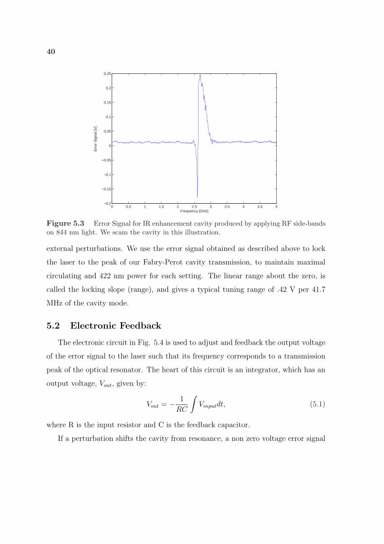
40
0 0.5 1 1.5 2 2.5 3 3.5 4 4.5 5−0.2
−0.15
−0.1
−0.05
0
0.05
0.1
0.15
0.2
0.25
Frequency [GHz]
Err
or S
igna
l [V
]
Figure 5.3 Error Signal for IR enhancement cavity produced by applying RF side-bandson 844 nm light. We scam the cavity in this illustration.
external perturbations. We use the error signal obtained as described above to lock
the laser to the peak of our Fabry-Perot cavity transmission, to maintain maximal
circulating and 422 nm power for each setting. The linear range about the zero, is
called the locking slope (range), and gives a typical tuning range of .42 V per 41.7
MHz of the cavity mode.
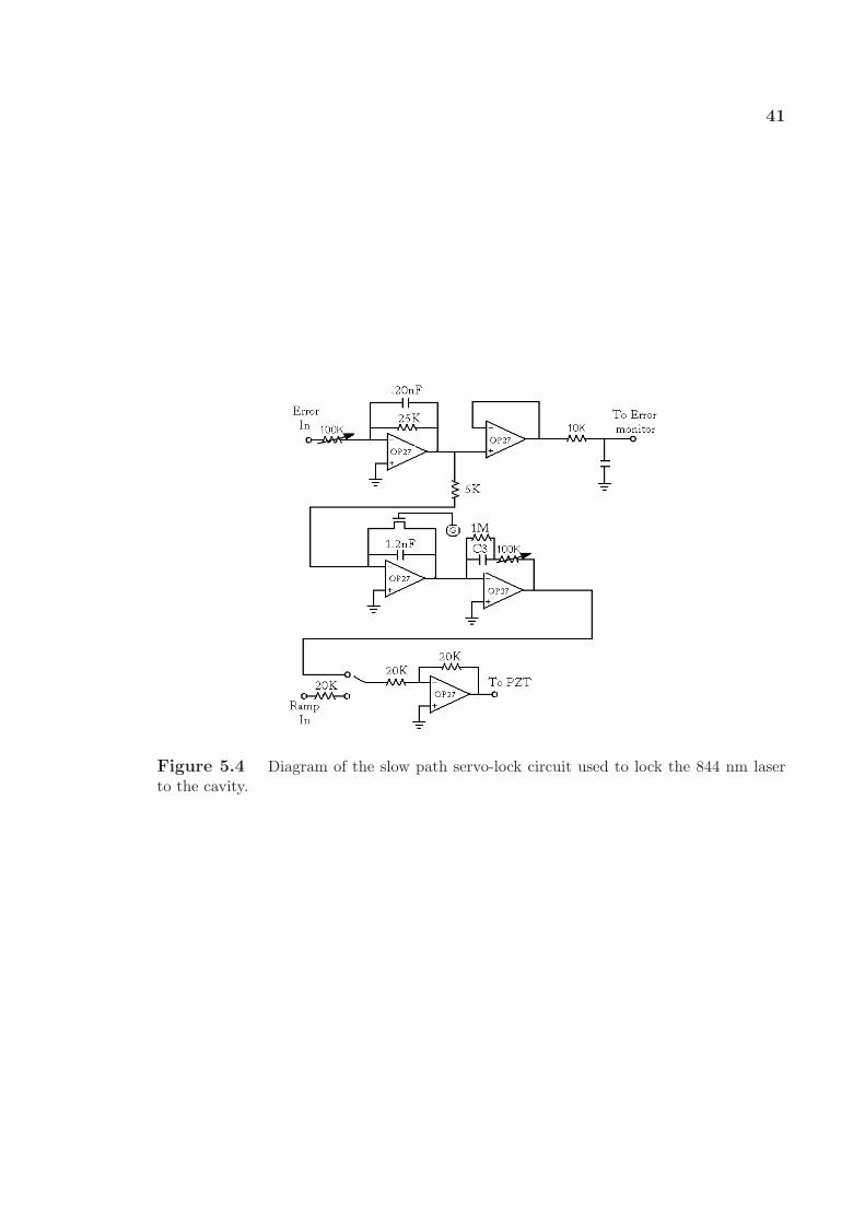
5.2 Electronic Feedback
The electronic circuit in Fig. 5.4 is used to adjust and feedback the output voltage
of the error signal to the laser such that its frequency corresponds to a transmission
peak of the optical resonator. The heart of this circuit is an integrator, which has an
output voltage, Vout, given by:
Vout = − 1
RC
∫Vinputdt, (5.1)
where R is the input resistor and C is the feedback capacitor.
If a perturbation shifts the cavity from resonance, a non zero voltage error signal
41
Figure 5.4 Diagram of the slow path servo-lock circuit used to lock the 844 nm laserto the cavity.
42
will be supplied to the integrator. For this input signal, the integrator’s output signal
rises steadily (integration over time). The rising output signal is amplified by the
output stage of the servo-lock circuit in a Fig. 5.4 and is fed back into the commercial
844 nm laser driving PZT (input control), which sweeps the laser frequency back to
the cavity resonance condition. As the laser frequency approaches the resonance
condition, the error signal reaches zero volt. The integrator now maintains a zero
volt output level, until another disturbance occurs.
5.3 Procedure to lock the laser
First, the initial settings are such that the servo loop in Fig. 5.4 is open, and only
a ramp voltage from a function generator is applied to the Ramp In input, which is
fed to the PZT to scan the optical resonator. Next, we reduce our scan to zero, and
adjusts the PZT Offset (not shown) until we see resonance phenomena of our cavity.
This centers the laser on the cavity resonance such that it falls within the circuit’s
lock range. Then we close the servo loop by switching the servo electronics from scan
to lock mode and monitor the error signal (which is at zero volts). The servo loop
will lock at the peak of the cavity transmission. Finally, we optimize the gain, G, of
the output signal to the PZT control to get a tight lock.
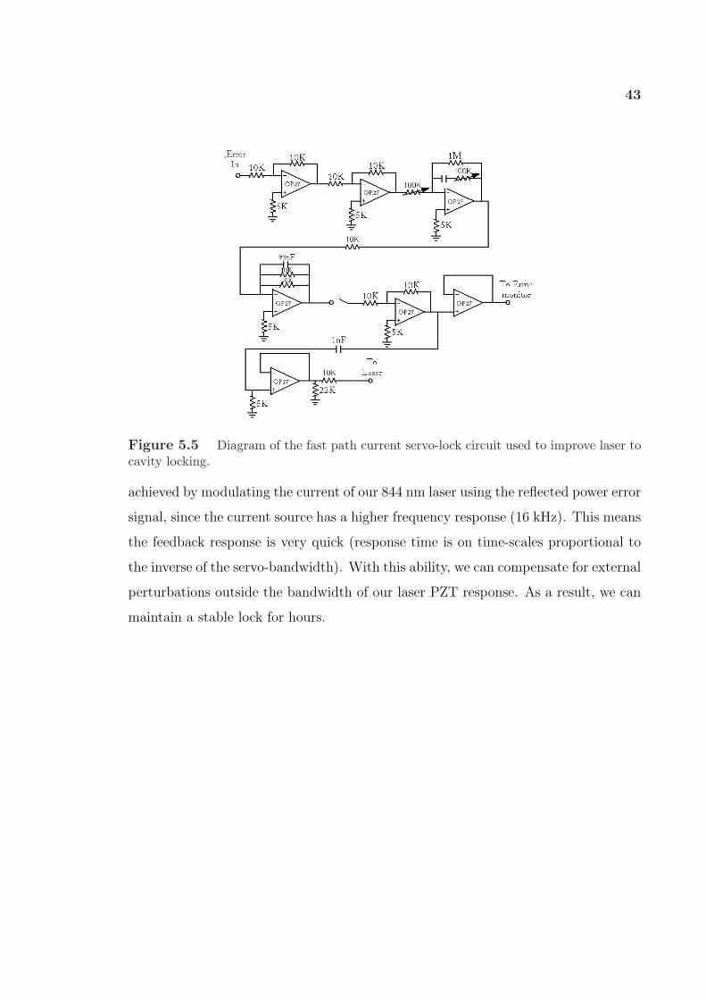
5.4 Lock Improvements
We had to include an additional servo network, to achieve robust laser to cavity
locking. The slow path feedback circuit, Fig. 5.4, controls the frequency of the laser
using a PZT actuator that has a large frequency to voltage excursion (MHzV
), but slow
response time. The slow response time of the PZT makes the servo loop of Fig. 5.4
inadequate for maintaining stable locking of our system, which is in the presence of
acoustic vibrations with frequencies higher than the response frequency of the 844 nm
laser’s PZT. The servo loop illustrated in Fig. 5.5 has a much faster response time
than the slow path servo loop of Fig. 5.5. The faster response time of this network is
43
Figure 5.5 Diagram of the fast path current servo-lock circuit used to improve laser tocavity locking.
achieved by modulating the current of our 844 nm laser using the reflected power error
signal, since the current source has a higher frequency response (16 kHz). This means
the feedback response is very quick (response time is on time-scales proportional to
the inverse of the servo-bandwidth). With this ability, we can compensate for external
perturbations outside the bandwidth of our laser PZT response. As a result, we can
maintain a stable lock for hours.
Chapter 6
Conclusions
6.1 Summary
We have illustrated the necessary steps for constructing a intensity stabilized
blue laser source at 421.7 nm. We have explained the nonlinear optical concepts
needed to make such a laser possible. Also, we described the use and purpose of an
optical resonator in constructing such a laser. We typically run our blue laser with
approximately 9 mW of light and we lock it to a strontium ion transition line for
frequency stabilization. About 1 mW is used to optically image ultracold plasmas in
our lab. This signifies the beginning of the use of a new and powerful technique to
study ultracold plasmas [33].
6.2 Improvements
Figure 4.10 illustrates that the amount of harmonic power increase linearly with
the fundamental power. Thus, as indicated by the figure, for higher input powers we
should obtain more blue. Unfortunately, our system will be unable to behave in this
manner, since our lock becomes unstable at these higher input powers. We believe
this instability in our lock is a result of having a small cavity length.
For instance, for more power circulating in the cavity there is a corresponding
increase in the crystals temperature. This increase in temperature causes a change
in the crystal’s optical path length. Since the crystal is about 20% of the cavity
length, this effect alters the resonant frequency of cavity. In turn, the longitudinal
mode of the cavity shifts, thereby causing our lock to come out of the locking range.
However, if we can make the total cavity length much larger the length of the doubling
crystal, our system will become more insensitive to changes in crystal length, therefore
allowing us to achieve stability in our lock for higher input fundamental powers.
45
6.3 Future Experiments
The future use for this laser system is vast. We are currently using our blue laser
source to image and measure the ion absorption spectrum. We are planing to use our
laser to study ion acoustic waves, for determining the temperature of the electrons in
the plasma. Further, the ultimate goal, is to use our blue laser source to laser cool
and trap our ultracold neutral plasma. The ability to do this will allow us to access
regimes in plasma physics not yet explored.
Appendix A
Circulating Power
The circulating power for our system can be determined by solving Eq. 3.1 by
means of a series of successive or iterative approximations. The zero-order solution
of Eq. 3.1 is given by:
P 0c =
(1−Ra)Pinput
[1−√
RaRb(1− `− 0)]2(A.1)
The first-order solution P 1c is obtained by inserting P 0
c in the expression for C=ξnLPc
in Eq. 3.1:
P 1c =
(1−Ra)Pinput
[1−√
RaRb(1− `− ξnL[(1−Ra)Pinput
[1−√
RaRb(1−`−0)]2])]2
. (A.2)
The second order term is obtain by inserting Eq. A.2 into Eq. 3.1. Continuing in
this manner, we obtained Pc to the forth order.
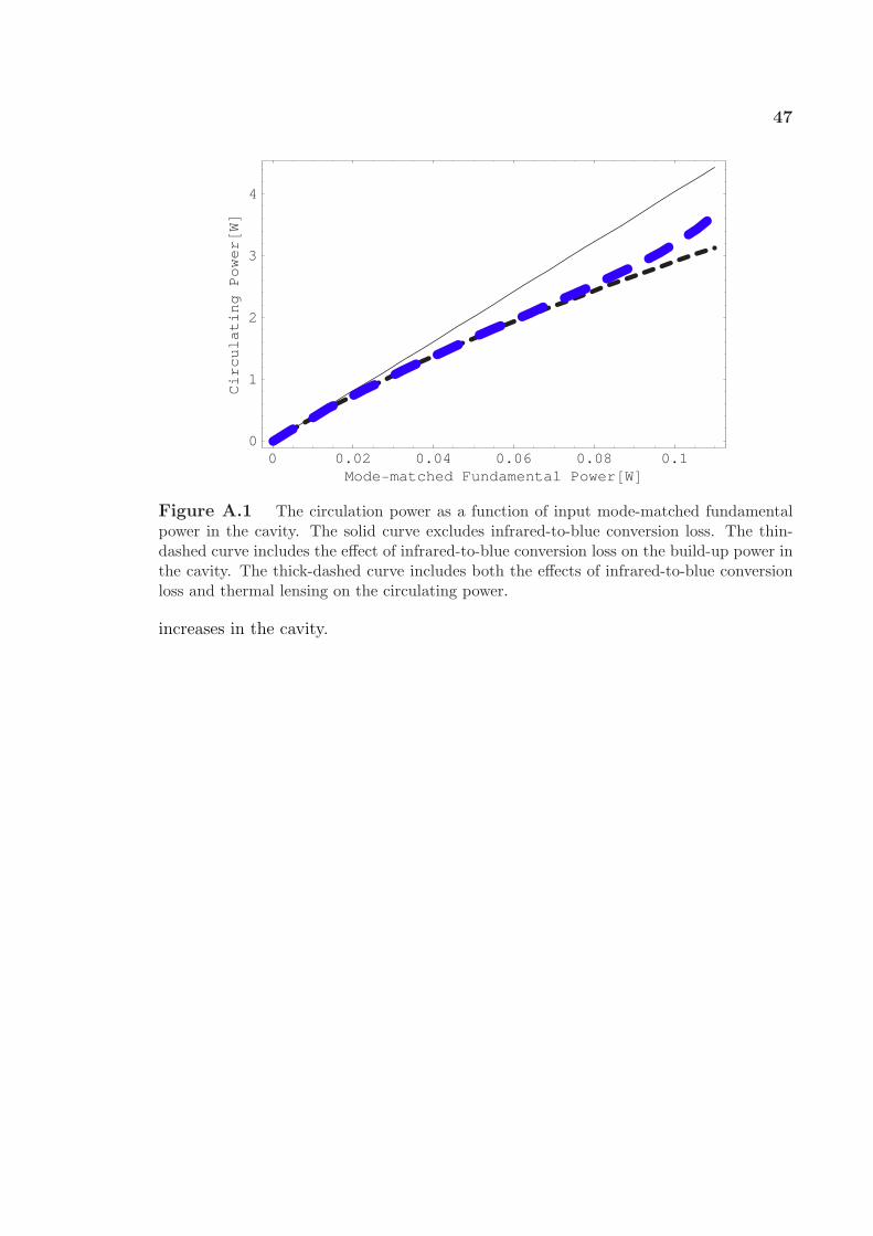
Figure A.1 is a plot of the circulating power as a function of input mode-matched
fundamental power in the cavity. The solid curve is a plot of Eq. 3.1 with C = 0
(zero-order approximation). For 100 mW of mode-matched fundamental power input
we obtain a peak circulating power of 4.4 W.
The thin-dashed curve in Fig. A.1 is a plot of Eq. 3.1 approximated to the
forth-order. The value of ξnL is .004/W. For fundamental powers greater than 30
mW, infrared-to-blue conversion loss reduces the amount of power circulating in the
cavity. The peak value of circulating power for this case is 3.2 W.
The thick-dashed curve in Fig. A.1 is a plot of Eq. 3.1 approximated to the
forth-order including the effect of thermal lensing. The deviation between this curve
and the thin-dashed curve occurs for input powers greater than 80 mW, and is a
consequence of increase in the resonator beam waist size, s2, inside the cavity. The
increase in s2 causes ξnL to reduce in magnitude, which in turn decreases the fraction
of infrared power converted to blue. As a result, the amount of circulating power
47
0 0.02 0.04 0.06 0.08 0.1Mode-matched Fundamental Power@WD
0
1
2
3
4
CirculatingPower@WD
Figure A.1 The circulation power as a function of input mode-matched fundamentalpower in the cavity. The solid curve excludes infrared-to-blue conversion loss. The thin-dashed curve includes the effect of infrared-to-blue conversion loss on the build-up power inthe cavity. The thick-dashed curve includes both the effects of infrared-to-blue conversionloss and thermal lensing on the circulating power.
increases in the cavity.
48
References
1. H. J. Metcalf and P. v. d Straten, Laser Cooling and Trapping. Springer, New
York, first edition (1969).
2. S. Ichimaru, Rev. Mod. Phys. 54, 1017 (1982).
3. P. Mansbach and J. Keck, Phys. Rev. 181, 275 (1969).
4. M. S. Murillo, Phys. Rev. Lett. 87, 115003 (2001).
5. T. C. Killian, S. Kulin, S. D. Bergerson, L. A. Orozco, C. Orzel, and S. L.
Rolston. “Creation of an Ultracold Neutral Plasma”, Phys. Rev. Lett. 83, 4776
(1999).
6. S. Kulin, T. C. Killian, S. D. Bergerson, and S. L. Rolston. “Plasma Oscillations
and Expansion of an Ultracold Neutral Plasma”, Phys. Rev. Lett. 85, 318 (1999).
7. K. J. Kuhn, Laser Engineering. Pretice-Hall, Inc., New Jersey, first edition
(1975).
8. Ivan Biaggio, P. Kerkoc, L. S. Wu, and Peter Gunter. “Refractive indices of
orthorhombic KNbO3. II. Phase-matching configurations for nonlinear-optical
interactions”, J. Opt. Soc. Am. B 9, 4 April (1992).
9. V. G. Dmitrev, G. G. Gurzadyan, and D. N. Nikogosyan. Handbook of Nonlinear
Optical Crystals, Springer-Verlag, volume 64, Berlin, (1975).
10. Y. Uematsu, “Nonlinear Optical Properties of KNbO3 single crystal in the
orthorhombic phase”, Jpn. J. Appl. Phys. 9, (3) 380–386 (1992).
11. H. Kogelnik and T. Li, Laser Beams and Resonators. Proceedings of the IEEE,
VOL. 54, NO. 10, OCTOBER (1966).
49
12. A. Maitland and M. H. Dunn, Laser Physics. John Wiley & Sons, Inc., New
York, first edition (1969).
13. B. E. A. Saleh and M. C. Teich, Fundamentals Of Photonics. John Wiley &
Sons, Inc., New York, (1991).
14. Anthony E. Siegman, Lasers. University Science Books, California, (1986).
15. Christoopher C. Davis, Laers and Electro-Optics. Cambridge University Press,
New York, (1996)
16. M. Bode, I. Freitag, A. Tunnermann, and H. Welling. “Frequency-tunable 500-
mW continous-wave all solid state single frequency source in the blue spectral
Region”, Opt. Lett. 22, (16) 14 August (1997).
17. M. Lodahl, J. L. Sorenson, and E.S. Polzik. “High efficency second harmonic
generation with a low power diode laser”, Appl. Phys. B 64, 383–386 (1997).
18. G. D. Boyd and D. A. Kleinman “Parametric interaction of focused guassian
light beams”, J. Appl. Phys. 39, 3597 (1968).
19. H. Mabuchi, E. S. Polzik, and H. J. Kimble “Blue-light-induced infrared absorp-
tion in KNBO3”, J. Opt. Soc. Am. B 11, 2023–2029 (1994).
20. L. E. Busse, L. Goldberg, and M. R. Surette, “Absorption losses in MgO-doped
and undoped potassium niobate”, J. Appl. Phys. 75, 1102–1110 (1994).
21. Bruce G Klappauf. “Detailed Study of eficent blue laser source by second har-
monic generation in a semi-monolithic cavity semi-monolithic cavity for cooling
of strontium atoms”, Opt. Soc. Am., (2003).
22. A. D. Ludlow, H. M. Nelson, and S.D. Bergson. “Two-photon absorption in
potassium niobate”, electronic pre-prints.
50
23. E .S. Polzik and H.J. Kimble, “Frequency doubling with KNbO3 in an external
cavity”, Opt. Lett 16, (18) 15 Setember (1991).
24. M. Abramowitz and I. A. Stegun, Handbook of Mathematical Functions. Dover,
New York, (1970), p. 228.
25. Gorachand Ghosh. “Dispersion of thermo-optic coefficients in a potassium nio-
bate nonlinear crystal”, Appl. Phys. Lett. 65, (26) 26 December (1994).
26. A. Yariv. Quantum Electronics. John Wiley & Sons, Inc., New York, second
edition (1975).
27. P. Dube, L. -S. Ma, J. Ye, P. Junger, and J. L. Hall. “Thermally induced self-
locking of an optical cavity by overtone absorption in acetylene gas”, J. Opt.
Soc. Am. B 13, (9) 9 September (1996).
28. P. W. P. Drever et al. “Laser Phase and Frequency Stabilization Using an Optical
Resonator”, Appl. Phys. B 31, 97–105 (1983).
29. G. C. Bjorklund et al. “Frequency-modulation (FM) Spectroscopy-Theory of
Line Shapes and Signal-to-noise Analysis”, Appl. Phys. B 31, 145 (1983).
30. M. L. Boas, Mathematical Methods In The Physical Sciences. John Wiley &
Sons, New York, second edition (1970), p. 509.
31. J. M. W Kruger. A Novel Technique For Frequency Stabilizing Laser Diodes.
M.S., University of Otago (1998).
32. Paul Horowitz and Winfield Hill, The Art of Electronics. Cambridge University
Press, New York, second edition (1989).
51
33. C. E. Simien, Y. C. Chen, P. Gupta, S. Laha, Y. N. Martinez, P. G. Mickel-
son, S. B. Nagel, and T. C. Killian. “Using Absorption Imaging to Study Ion
Dynamics in an Ultracold Neutral Plasma”, Phys. Rev. Lett. 92, 143001 (2004).