algebraic topology
DESCRIPTION
Part III Lecture NotesTRANSCRIPT

Algebraic Topology by Will Merry
Lecture notes based on the Algebraic Topology course lectured by Dr. I. Smith inMichaelmas term 2007 for Part III of the Cambridge Mathematical Tripos.
Contents
1 Introduction . . . . . . . . . . . . . . . . . . . . . . . . . . . . . . . . 12 Singular cohomology . . . . . . . . . . . . . . . . . . . . . . . . . . . . 33 Exact sequences . . . . . . . . . . . . . . . . . . . . . . . . . . . . . . 104 Degrees . . . . . . . . . . . . . . . . . . . . . . . . . . . . . . . . . . . 205 Cell complexes . . . . . . . . . . . . . . . . . . . . . . . . . . . . . . . 246 Generalised cohomology theories . . . . . . . . . . . . . . . . . . . . . . 367 The cohomology ring . . . . . . . . . . . . . . . . . . . . . . . . . . . 408 Interlude: categories and cup length . . . . . . . . . . . . . . . . . . . . 459 Cohomology of manifolds . . . . . . . . . . . . . . . . . . . . . . . . . 4710 Poincaré duality . . . . . . . . . . . . . . . . . . . . . . . . . . . . . . 6011 The Thom isomorphism theorem . . . . . . . . . . . . . . . . . . . . . 6612 The diagonal cohomology class . . . . . . . . . . . . . . . . . . . . . . 75
Please let me know on [email protected] if you find any errors - I’m sure there are many!
1 Introduction
Much of what follows is almost entirely stolen from the excellent book ‘Algebraic Topology’ byAllen Hatcher. I have also borrowed heavily from ’Differential Forms in Algebraic Topology’by Raoul Bott and Loring Tu. The reader is strongly referred to either of these texts for furtherinformation and clarification.
1.1 DefinitionA topological space X is simply connected if any two maps (note: in the context of topologicalspaces, map means continuous function in this course) S1 → X can be continuously deformed intoeach other.
1.2 Winding numbersIt can be shown that R2 is simply connected but R2\0 is not. In fact, from elementary complexanalysis, a closed loop γ : S1 → R2\0 has a winding number, deg(γ) ∈ Z, which is invariantunder continuous deformations, such that the loop γn : t 7→ (cos 2πnt, sin 2πnt) has degree n.
The existence of a winding number allows us to give an easy topological proof of the fundamentaltheorem of algebra.
1

1 Introduction 2
1.3 Corollary (The fundamental theorem of algebra)If f(z) ∈ C[z] has positive degree then f has a root.
J We may take f monic. Suppose f(z) 6= 0 for all z ∈ C. Let γR := f(Reiπt) : S1 → R2\0.If R = 0, then γ0 is a constant and has degree zero. Now take R > |a1| + · · · + |an| (wheref(z) = zn + a1z
n−1 + · · · + an) and consider γR,s(t) := zn + s(a1zn−1 + · · · + an)
∣∣z=Reiπt
. ThenγR,0 = γn, which has degree n, and γR,1 = γR. The choice of R implies γR,s 6= 0 for all s ∈ I(where as always, we take I = [0, 1]) and thus we can continuously deform γR,0 to γR,1 in R2\0.Then the deformations γn = γR,0 γR,1 = γR γ0 imply n = 0, that is, f is a constant. I
1.4 Higher dimensionsThe next natural generalization is to consider maps Sn → X. We find that any 2 maps Sn →Rn+1 can be continuously deformed into each other, but the same is not true for any two mapsSn → Rn+1\0. In fact, (this will get proved in Chapter 4) any map γ : Sn → Rn+1\0 hasa well defined degree; an integer deg(γ) which is again invariant under continuous deformations,such that a constant map has degree zero and the inclusion i : Sn → Rn+1\0 has degree 1.
This time the existence of a degree satisfying the above properties allows us to give a simpleproof of Brower’s fixed point theorem.
1.5 Corollary (Brower’s fixed-point theorem)Any map f : Dn → Dn has a fixed point (where Dn = x ∈ Rn | |x| ≤ 1).
J Suppose not. Given r, s ∈ I := [0, 1], we want to define a map γr,s : Sn−1 → Sn−1 sending
x 7→ rx− sf(rx)|rx− sf(rx)|
. (1)
Unfortunately (1) is not well defined for all values of r and s in I. Luckily however γt,0 is welldefined for all t ∈ I with γ0,1 the constant map c : x 7→ f(0)
‖f(0)‖ which has degree zero. Moreoverγ1,s is well defined for all s ∈ I, since for s = 1, x − f(x) 6= 0 for all x ∈ Sn−1 by assumption,and if s < 1 then since x ∈ Sn−1 and f(Dn) ⊆ Dn we also have x − sf(x) 6= 0. Note thatγ1,0 = i is the inclusion map which has degree one and γ1,1 = γ1. But then the deformationsi = γ1,0 γ1,1 γ0,1 = c contradict the invariance the degree under continuous deformations. I
1.6 DefinitionWe say two spaces X,Y are homotopy equivalent if there exists maps f : X → Y , g : Y → Xsuch that fg is homotopic to 1Y (written fg ' 1Y ) and gf ' 1X . We write X ' Y .
Sn and Rn+1\0 are homotopy equivalent, via the inclusion i : Sn → Rn+1\0 and the mapr : Rn+1\0 → Sn sending x 7→ x
|x| . Indeed, ri = 1Sn and ir ' 1Rn+1\0, via the linear homotopy(x, t) 7→ tx+ (1− t) x
|x| .
1.7 The goal of algebraic topologyIn general, given two spaces X and Y , it is easy to prove that X and Y are homotopic (just exhibitan explicit homotopy equivalence) but much more difficult to prove they are not homotopic; howdo you prove no such homotopy equivalence exists?
Broadly speaking, algebraic topology is about assigning algebraic structures to topologicalspaces in such a way that homotopic spaces are assigned the same structure1In theory this shouldgives us an easy way of telling whether two spaces are not homotopic; if the associated algebraicinvariants are not the same then they cannot be homotopic. We saw this method in action above:
1 Put more eloquently (but much less intelligibly), we will construct various functors from the category of htopof topological spaces and homotopy classes of maps to some algebraic category.
2 Singular cohomology 3
both of the two proofs above obtained their desired contradiction in this way. In fact, the invariantwe assumed the existence of in the proof of Corollary 1.5, the degree is a particularly importanttool we shall study in Chapter 4.
1.8 Homotopy groupsHere is another example of an homotopy invariant one can associate to a space X. One can showthat the set C0((Sk, 1)), (X,x0))/ ∼ of maps Sk → X that send 1 to x0, modulo homotopy) forms agroup πk(X,x0), the kth homotopy group of X, such that if X ∼= Y then πk (X,x0) ∼= πk (Y, y0).Unfortunately the homotopy groups of a topological space are in general are very hard to compute;they are not yet completely known for S2!
In this course we will study a different type of invariant; various homology and cohomologytheories. These are in general much harder to define (it will take us most of Chapter 2 to do so)but much easier to compute.
2 Singular cohomology
2.1 DefinitionA chain complex (C∗, d) is a sequence of abelian groups and homomorphisms (called differen-tials) indexed by Z,
· · · → Cn+1d→ Cn
d→ Cn−1 → . . . ,
such that at each stage d d = 0. The homology H∗(C∗, d) of the chain complex is the sequenceof abelian groups
Hn(C, d) :=ker d : Cn → Cn−1
im d : Cn+1 → Cn.
Elements of Zn := ker d : Cn → Cn−1 are called n-cycles and elements of Bn := im d :Cn+1 → Cn are called n-boundaries.
2.2 DefinitionA cochain complex (C∗, δ) is a sequence of abelian groups and homomorphisms (called codif-ferentials) indexed by Z,
· · · → Cn−1 δ→ Cnδ→ Cn+1 → . . . ,
such that at each stage δ δ = 0. The cohomology2 H∗(C∗, δ) of the chain complex is thesequence of abelian groups
Hn(C, δ) :=ker δ : Cn → Cn+1
im δ : Cn−1 → Cn.
Elements of Zn := ker δ : Cn → Cn+1 are called n-cocycles and elements of Bn := im δ :Cn−1 → Cn are called n-coboundaries.
2.3 DefintionsAn n simplex is the convex hull of n + 1 ordered points v0, . . . , vn in some Euclidean space Rmsuch that the vectors vi − v0 are linearly independent for i = 1 . . . n. For an n simplex s, we writes = [v0, . . . , vn] to indicate that s has ordered vertices v0, . . . , vn.
The standard n simplex is
∆n :=
t ∈ Rn+1
∣∣∣ n∑i=0
ti = 1, ti ≥ 0
.
2 Throughout the notes, when we are talking about both homology and cohomology at the same time we willoccasionally say ‘cohomology’ to mean ‘both homology and cohomology’. An example of this is the title of thischapter is ‘Singular cohomology’.

2 Singular cohomology 4
Any n simplex s = [v0, . . . , vn] is canonically the image of ∆n under a linear homeomorphism∆n → s sending t = (ti) 7→
∑n+1i=0 tivi.
The faces of an n simplex [v0, . . . , vn] are the images of ∆n−1 ⊆ ∆n under this homeomorphismobtained by setting ti = 0; thus each face is an (n− 1)-simplex, and we write the ith face as[v0, . . . , vi, . . . , vn]. We orient each edge of an n simplex [v0, . . . , vn] in the obvious way (namely,an edge vivj points from vi to vj if and only if i < j), and this ordering is compatible with passingto faces, in the sense that each edge in a given face retains the orientation it had in the parentsimplex.
If X is a topological space an n-simplex in X is a continuous map σ : s→ X, where s is ann-simplex.
Actually it is often notationally convenient to view an n-simplex in X as a continuous mapσ : ∆n → X; this is no problem as any n-simplex is homeomorphic to ∆n.
2.4 DefinitionLet X be a topological space. The singular chain complex C∗(X) is defined by setting Cn(X)to be the free abelian group on all n-simplices in X, that is
Cn(X) =
N∑i=1
hiσi
∣∣∣σi : ∆n → X continuous, hi ∈ Z, N ∈ N
,
and then defining the differential d : Cn(X)→ Cn−1(X) by
d(σ) :=n∑i=0
(−1)iσ|[v0,...,vi,...,vn]
and then extending by linearity across Cn(X). We write H∗ (X) for the associated singularhomology H∗ (C∗ (X) , d) of X.
To check that this does indeed define a chain complex, we need to check that d is in fact adifferential, that is:
2.5 LemmaFor C∗(X) and d as defined above we have d2 = 0.
J It is enough to show that d(dσ) = 0 for some n-simplex σ : ∆n → X. To see this, observe:
d(dσ) =n∑i=0
(−1)id(σ|[v0,...,vi,...,vn])
=∑j<i
(−1)i(−1)jσ|[v0,...,vj ,...,vi,...,vn] +∑j>i
(−1)i(−1)j−1σ|[v0,...,vi,...,vj ,...,vn],
and this is equal to zero, since every term cancels. I
The construction of the singular cochain complex from the singular chain complex is actuallya general algebraic device which we now describe.
2.6 DefinitionLet (C∗, d) be a chain complex, and G an abelian group. Set Cn := Hom(Cn, G), the dual cochaingroup of Cn and let δ : Cn → Cn+1 be the dual homomophism defined by δ(ϕ)(x) = ϕ(d(x)).Since d2 = 0 we have δ2(ϕ)(x) = ϕ(d2(x)) = 0 and thus δ2 = 0. Thus we obtain a dual cochaincomplex (C∗, δ) and we can define the the cohomology groups H∗(C;G). We call H∗ (C;G) thecohomology of C∗ with coefficients in G.
2 Singular cohomology 5
2.7 RemarkOne can show that the cohomology groups Hn(C;G) are determined solely by G and the homologygroups Hn(C) of (C∗, d); this is the universal coefficient theorem for cohomology. Theprecise statement is the following:
Hn (C;G) ∼= Hom (Hn (C) , G)⊕ Ext (Hn−1 (C) , G) .
In this course we will not prove this result (we shall not even give a definition of the Ext functorthat appears in the above equation). However in Chapter 5 we will prove a special case of thisresult applicable to cell complexes - see Theorem 5.29 below, and in Lemma 2.8 below we exhibita surjective map h : Hn (C;G)→ Hom (Hn (C) , G).
2.8 LemmaLet (C∗, d) be a chain complex, G an abelian group and (C∗, δ) the corresponding dual cochaincomplex. Then there exists a canonical surjective map h : Hn (C;G) → Hom (Hn (C) , G) givenby evaluating cocycles on cycles.
J Here and elsewhere we let [ϕ] denote the cohomology class of an element ϕ ∈ Zn, andsimilarly for homology classes. We want to define h : Hn (C;G)→ Hom (Hn (C) , G) by
h ([ϕ]) ([σ]) := ϕ (σ) , [ϕ] ∈ Hn (C) , [σ] ∈ Hn (C) .
To check this is well defined suppose ϕ′ ∈ Zn and σ′ ∈ Zn are different representatives of [ϕ] and[σ] respectively. Then ϕ′ = ϕ+ δψ and σ = σ + dτ for some ψ ∈ Cn−1 and τ ∈ Cn+1. Then
ϕ′ (σ′) = (ϕ+ δψ) (σ + dτ)= ϕ(σ) + ϕ (dτ) + δψ (σ) + δψ (dτ)= ϕ (σ) + δϕ (τ) + ψ (dσ) + ψ
(d2τ)
= ϕ (σ) + 0,
since by assumption δϕ = 0, dσ = 0 and of course d2τ = 0. Thus h is well defined.It remains to check h surjects. Here we use the fact that Bn is a free abelian group (being
a subgroup of the free abelian group Cn), and hence the splitting lemma (Proposition 5.27) ofChapter 5 below gives the existence of a map p : Cn → Zn such that p|Zn = 1. We will use theexistence of this map to define a right inverse j for h, thus proving h surjects.
If ϕ ∈ Hom (Hn (C) , G) then we may view ϕ as a homomorphism Zn → G that vanishes onBn, and then ϕp : Cn → G is an element of Cn that vanishes on Zn, that is, ϕp ∈ Zn. Finally ifq : Zn → Hn (C) is the natural quotient map, define j : Hom (Hn (C) , G)→ Hn (C) by
j (ϕ) := q (ϕp) .
Since clearly hj = 1, this completes the proof. I
2.9 AddendumSuppose in addition that Hn−1 (C) is zero or free. Then h is also injective, and hence we have acanonical isomorphism
Hn (C) ∼= Hom (Hn (C) , G) .
J Suppose h ([ϕ]) = 0. Let ϕ ∈ Zn (C) be a representative of [ϕ]. Then the compositionϕd−1 : Bn−1 (C) → G is well defined. Since Hn−1 (C) = Zn−1 (C) /Bn−1 (C) is assumed to befree, it follows Bn−1 (C) is a direct summand of Zn−1 (C), and hence also of Cn−1 (this again usesthe splitting lemma (Proposition 5.27). Thus there exists a map t : Cn−1 → Bn−1 (C) such thatt|Bn−1(C) = 1. Now set ψ := ϕd−1t : Cn−1 → G. Then
δψ ([σ]) = ψ (d [σ]) = ϕ ([σ]) ,
and thus δψ = ϕ and so [ϕ] = 0. I
2 Singular cohomology 6
2.10 DefinitionThe singular cochain complex (C∗(X; Z), δ) is the cochain complex obtained by taking (C∗, d) =(C∗ (X) , d) and G = Z in Definition 2.6. We write H∗ (X; Z) for the associated singular coho-mology of X.
Where no confusion is possible, we omit the coefficients ‘Z’ from the notation for simplicity,and write H∗ (X) instead of H∗ (X; Z). Occasionally this will not be possible.
2.11 DefinitionLet (C∗, d) and (D∗, d′) be chain complexes. A chain map is a map f∗ : C∗ → D∗, that is, acollection of linear homomorphisms fn : Dn → Dn that commute with the differentials: f∗d = d′f∗. In other words, the following commutes:
Cn
d
f∗ // Dn
Cn−1f∗
// Dn−1
d′
OO
A chain map f∗ induces a map (also called) f∗ : H∗ (C)→ H∗ (D) in the obvious way:
f∗ ([σ]) := [f∗ (σ)] .
It is precisely the fact that f∗ commutes with the differentials that makes this well defined. Indeed,f∗ (σ) does indeed represent a cohomology class in Hn (D) since
d (f∗ (σ)) = f∗ (dσ)= f∗ (0) = 0,
and if σ′ also represents [σ], so σ′ = σ + dτ then
f∗ (σ′) = f∗ (σ + dτ)= f∗ (σ) + f∗ (dτ)= f∗ (σ) + d (f∗ (τ)) ,
and hence [f∗ (σ)] = [f∗ (σ′)].
2.12 DefinitionIn an entirely similar way we define a cochain map f∗ : C∗ → D∗ between cochain complexes(C∗, δ) and (D∗, δ′) to be a collection of maps fn : Cn → Dn such that δf∗ = f∗δ′:
Cn+1f∗ // Dn+1
Cn
δ
OO
f∗// Dn
δ′
OO
Similarly to the case of a chain map, a cochain map induces a well defined map f∗ : H∗ (C) →H∗ (D) in cohomology given by
f∗ ([ϕ]) = [f∗ (ϕ)] .

2 Singular cohomology 7
2.13 Cohomology is functorialLet f : X → Y be continuous. Given an n-simplex σ : ∆n → X, we can define an n-simplex in Yas fσ : ∆n → Y . In this way we obtain a map f∗ : C∗(X)→ C∗(Y ). Moreover, f∗ is a chain map.Indeed, if σ : ∆n → X is an n-simplex both sides evaluate on σ to give
n∑i=0
(−1)ifσ|[v0,...,vi,...,vn].
Thus f∗ defines a map H∗ (X)→ H∗ (Y ).Similarly we can define a map f∗ : C∗(X)→ C∗(Y ) be defining f∗(ϕ)(σ) = ϕ(f∗(σ)). Moreover
we have
δ(f∗ϕ)(σ) = f∗(ϕ)(dσ)= ϕ(f∗dσ)= ϕ(df∗(σ))= δ(ϕ(f∗σ))= f∗(δϕ(σ)),
and hence f∗ is a cochain map. Thus f∗ also descends to a well defined map f∗ : H∗(X)→ H∗(Y ).
2.14 CorollarySingular homology and singular cohomology is a homeomorphism invariant.
J One then easily checks that
1∗ = 1, (fg)∗ = f∗g∗,
in3 particular this shows that if X is homeomorphic to Y via f , then H∗(X) ∼= H∗ (Y ), via theisomorphism f∗.
Similarly it is easy to see1∗ = 1, (fg)∗ = g∗f∗,
and so4 similarly if X is homeomorphic to Y via f , then H∗(Y ) ∼= H∗ (X), via the isomorphismf∗. I
2.15 ExampleWe compute H∗(pt) and H∗(pt) (where pt is a space consisting of a single point). For each n, thereis a unique continuous map σ : ∆n → pt, namely the constant map. Hence the chain complexC∗(pt) is very simple:
. . .0→ Z ±1→ Z 0→ Z ±1→ Z→ 0,
and this immediately gives Hn(pt) = 0 for n 6= 0 and H0(pt) = Z. Dualizing, we obtain exactlythe same result for H∗(pt).
2.16 PropositionLet X be a topological space. Then H0(X) = H0(X) = Zn, where n is the number of path com-ponents of X.
3 More precisely, this shows that H∗ is a covariant functor from the category of topological spaces top to thecategory of Z-graded abelian groups. It is much harder (see Theorem 2.17 below) to show that H∗ is indeed afunctor on htop, that is, if X is homotopy equivalent to Y then H∗ (X) ∼= H∗ (Y ).
4 This shows H∗ is a contravariant functor from the category of topological spaces top to the category of Z-gradedabelian groups. As with H∗, it is factor a functor on htop.

2 Singular cohomology 8
J It is immediate that if X =∐αXα then H∗(X) =
⊕αH∗(Xα) and H∗(X) =
⊕αH
∗(Xα),as im σ : ∆n → X is always contained in a single path component for continuous σ. Thus it isenough to show that for a path connected space X, we have H0(X) = H0(X) = Z.
So let X be path connected, and define a map ε : C0(X)→ Z by ε(∑hiσi) =
∑hi. Clearly ε is
surjective. Moreover, B0(X) ⊆ ker ε, as if τ : [v0, v1]→ X is a 1-simplex in X with τ (vi) =: xi ∈ Xthen if σi : ∆0 = pt → X has image xi ∈ X , we have ε(dτ) = ε(σ1 − σ0) = 1 − 1 = 0. Thusε descends to a well defined map ε : H0(X) → Z. We now show B0(X) = ker ε, so ε is anisomorphism.
Indeed, if ε(∑hiσi) = 0, pick a basepoint x0 ∈ X, write xi for the image of σi : ∆0 = pt→ X.
Then define τi : [v0, vi] → X by τi (vj) = xj (j = 0, i). Then d(∑hiτi) =
∑hiσi − (
∑hi)σ0,
where σ0 has image x0 . But∑hi = ε(
∑hiσi) = 0 and thus d(
∑hiτi) =
∑hiσi.
Thus H0(X) = Z. To prove the result for H0 (X), note that since a 0-simplex is just a point, acochain ϕ in C0(X) is just a (not necessarily continuous) function X → Z. The assertion δϕ = 0is equivalent to saying that ϕ is constant on path components of X. Thus H0(X) is the group ofall the functions from path components of X to Z. I
The next proof is the first real theorem in the course.
2.17 Theorem (homotopy invariance of singular cohomology)If f, g : X → Y are homotopic then f∗ = g∗ as maps H∗(X) → H∗(Y ) and f∗ = g∗ as mapsH∗(Y )→ H∗(X).
2.18 CorollaryIf X ' Y then H∗(X) = H∗(Y ) and H∗(X) = H∗(Y ).
The proof of Theorem 2.17 will take some time. We first make the definition:
2.19 DefinitionLet C∗ and D∗ be chain complexes and f∗, g∗ : C∗ → D∗ chain maps. We say f∗ and g∗ are chainhomotopic if there exists a chain homotopy P : Cn → Dn+1 such that dP ± Pd = f∗ − g∗.Similary if C∗ and D∗ are cochain complexes and f∗, g∗ : C∗ → D∗ are cochain maps then we sayf∗ and g∗ are cochain homotopic if there exists a cochain homotopy Q : Cn → Dn−1 suchthat Qδ ± δQ = f∗ − g∗.
The point of these definitions is:
2.20 LemmaIf f∗, g∗ are chain homotopic then the induced maps on homology coincide. Similarly if f∗ and g∗are cochain homotopic then the induced maps on cohomology coincide.
J If dσ = 0 then
f∗ ([σ])− g∗ ([σ]) = [(f∗ − g∗) (σ)]= [(dP ± Pd)(σ)]= [d (Pσ)] = 0.
The proof for cohomology is similar. I
Before we can prove Theorem 2.17 we need the following geometric lemma.

2 Singular cohomology 9
2.21 Lemma∆n × I is the untion of n+ 1 copies of ∆n+1.
J Let ϕi : ∆n → I denote the map sending (t0, . . . , tn) 7→∑j>i tj ; note ϕi is indeed a map into
I, as t ∈ ∆n implies∑ti = 1. Let Gi ⊆ ∆n× I denote the graph of ϕi, which is homeomorphic to
∆n by the projection ∆n× I → ∆n. Label the vertices at the ‘bottom’ of ∆n× I by v0, . . . , vn andthe vertices at the ‘top’ of ∆n×I by w0, . . . , wn. Then Gi is the n-simplex [v0, . . . , vi, wi+1, . . . , wn].
Gi lies ‘below’ Gi−1 as ϕi ≤ ϕi−1, and the region between Gi and Gi−1 is the (n+ 1)-simplex[v0, . . . , vi, wi, . . . , wn]; this is indeed an (n + 1)-simplex as wi is not in Gi and hence not in then-simplex [v0, . . . , vi, wi+1, . . . , wn].
Since 0 = ϕn ≤ ϕn−1 ≤ · · · ≤ ϕ0 ≤ ϕ−1 = 1 we conclude that ∆n × I is the union of theregions lying between the graphs Gi, and hence the union of the n+ 1 different (n + 1)-simplices[v0, . . . , vi, wi, . . . , wn], each intersecting the next in an n-simplex face. I
We can now complete the proof of Theorem 2.17.
J Proof of Theorem 2.17: we first reduce to a special case. If f, g : X → Y are homotopicthen there is a continuous map F : X × I → Y such that F |X×0 = f and F |X×1 = g. Leti0 : X → X × I be the inclusion x 7→ (x, 0) and i1 : X → X × I the inclusion x 7→ (x, 1). Thenf = Fi0 and g = Gi1 and thus f∗ = F∗i0∗ and g∗ = F∗i1∗ and thus it is enough to show thati0∗ = i1∗.
Define the prism operator P : Cn(X)→ Cn+1(Y ) by
Pσ =n∑i=1
(−1)i(σ × id)|[v0,...,vi,wi,...,wn].
Note that the previous lemma ensures that the definition makes sense.Then
dPσ =∑j≤i
(−1)i(−1)j(σ × id)|[v0,...,vj ,...,vi,wi,...,wn]
+∑j≥i
(−1)i(−1)j+1(σ × id)|[v0,...,vi,wi,...,wj ,...,wn].
The terms with i = j cancel except for the two terms i = j = 0 and i = j = n, which are
(σ × id)|[v0,w0,...,wn] and − (σ × id)|[v0,...,vn,wn];
these are precisely i0∗ (σ) and −i1∗ (σ). The terms with i 6= j are precisely −Pdσ, since
−Pdσ =∑i<j
(−1)i(−1)j(σ × id)|[v0,...,vi,wi,...,wj ,...,wn]
+∑i>j
(−1)i−1(−1)j(σ × id)|[v0,...,vj ,...vi,wi,...,wn].
Thus we have shown that dPσ+Pdσ = i0∗ (σ)− i1∗ (σ), and this completes the proof of homotopyinvariance for singular homology, in view of Lemma 2.20.
It is then easy to deduce the homotopy invariance for singular cohomology. As before we needonly show i∗0 = i∗1, and dualizing dP+Pd = i0∗−i1∗ , we obtain a mapQ such thatQδ+δQ = i∗0−i∗1.Again, by Lemma 2.20, this implies i∗0 = i∗1 and thus the proof is complete. I
2.22 ExampleRn is homotopy equivalent to pt via a linear homotopy, and thus
Hm(Rn) = Hm(Rn) =
Z m = n,
0 m 6= n.(2)

3 Exact sequences 10
3 Exact sequences
In this chapter we introduce some elementary homological algebra and then use this to deduce twoextremely important results: excision and the Mayer-Vietoris sequence.
3.1 DefinitionsAn exact sequence is a chain complex with trivial homology, that is, ker d = im d. A shortexact sequence is an exact sequence with only three non-zero groups:
0→ A∗α→ B∗
β→ C∗ → 0,
with α injective,β surjective and ker β = im α. A long exact sequence is a (possibly) infinitesequence exact sequence.
A short exact sequence of chain complexes 0 → A∗α→ B∗
β→ C∗ → 0 is a collection ofchain complexes such that every row is exact:
0 // An+1α //
d
Bn+1β //
d
Cn+1
d
// 0
0 // Anα //
d
Bnβ //
d
Cn
d
// 0
0 // An−1α // Bn−1
β // Cn−1// 0
3.2 Relative cohomologyLet A ⊆ X be a subspace. Observe that d : C∗(X) → C∗(X) preserves A, as if im σ ⊆ A theneach of its faces lie in A and thus im dσ ⊆ A. Hence if we define
Cn(X,A) := Cn(X)/Cn(A),
then d descends to give a differential d : Cn(X,A) → Cn−1(X,A) and thus we obtain a chaincomplex C∗(X,A) called the relative chain complex of A. The corresponding homology groupsH∗(X,A) are called the relative homology groups of A. S
To obtain the relative cohomology groups, we set
Cn (X,A) := Hom (Cn (X,A) ,Z) .
By restricting δ, we obtain coboundary maps δ : Cn (X,A) → Cn+1 (X,A), and thus this givesrise to the relative cohomology groups Hn (X,A).
By definition, the sequence
0→ C∗(A) i→ C∗(X)j→ C∗(X,A)→ 0 (3)
is clearly exact.We apply Hom (−,Z) (or Hom (−, G) if we are working with coefficients in any abelian group
G) to the short exact sequence (3) to obtain a sequence
0← Cn (A) i∗← Cn (X)j∗← Cn (X,A)← 0. (4)
We need to show (4) remains exact5.
J To show this we observe that the map i∗ restricts a cochain on X to a cochain on A,and hence for a function ϕ : Cn (X) → Z, i∗ (ϕ) is the function obtained by restricting the
5 This is not trivial, since the functor Hom (−, Z) is not flat; in general it is only exact on the left.
3 Exact sequences 11
domain of ϕ to Cn (A). Every function ψ : Cn (A) → Z can be obtained from as i∗ (ϕ) for afunction ϕ : Cn (X) → Z; simply set ψ to be zero outside A. Thus i∗ is surjective. Next, forϕ : Cn (X) → Z, we have i∗ (ϕ) = 0 if and only if ϕ ≡ 0 on A. Thus i∗ (ϕ) = 0 if and only if ϕfactors as a homomorphism Cn (X,A)→ Z. This gives exactness. I
3.3 Propositon (snake lemma)Let
0→ A∗α→ B∗
β→ C∗ → 0
be an exact sequence of chain complexes. Then there exists a well defined boundary map ∂ :Cn(C)→ Cn−1(A) such that we have a long exact sequence
· · · → Hn(A) α→ Hn(B)β→ Hn(C) ∂→ Hn−1(A)→ . . .
J Step 1: Defining ∂.First we define ∂. If [c] is a class in Hn(C), pick a representative c ∈ Zn(C). Then by exactness
at C∗, c = β(b) for some b ∈ Bn. But then β(db) = d(βb) = dc = 0. Hence db ∈ ker β, and thusby exactness at B∗, we have db = α(a) for some a ∈ An−1.
Next, α(da) = d(αa) = d(db) = 0 and thus a defines a class [a] ∈ Hn−1(A). We wish to define∂[c] = [a]. To check this is well defined, first note that by exactness at A∗, α is injective and thusa was completely determined by b.
Now b is not uniquely determined, but if we had chosen b′ instead of b, then β(b′−b) = c−c = 0,and thus β(b′−b) = α(a′). Hence db′ = db+d(b′−b) = α(a)+d(αa′) = α(a+da′), and [a−da′] = [a].
Finally, if we had chosen a different representative c′ of [c], then c′ = c+dc′′ for some c′′ ∈ Cn+1.But then writing c′′ = β(b′′), we have c′ = c + d(βb′′) = β(b + db′′), and then as db = d(b + db′′)we conclude that ∂ is indeed well defined.
Step 2: Checking exactness.It remains to check exactness in all three places. This means checking six things:
1. im α ⊆ ker β. Immediate as βα = 0⇒ β∗α∗ = 0.
2. ker β ⊆ im α. If β[b] = 0, then if b represents [b] then β(b) = dc for some c ∈ Cn+1. Butthen surjectivity of β gives c = β(b′) for some b′ ∈ Bn+1. Then β(b− db′) = β(b)− d(βb′) =β(b) − dc = 0. Thus b − db′ = α(a) for some a ∈ An. Next, α(da) = d(αa) = d(b − db′) =db = 0. Thus by injectivity of α, da = 0 and we so a represents some [a] ∈ Hn(A). Thenα[a] = [b− db′] = [b], and hence [b] ∈ im α.
3. im β ⊆ ker ∂. ∂β = 0, as if [c] = β[b] then if c represents [c], we can write c = β(b) for someb ∈ Bn such that db = 0. Tracing through, this gives ∂[c] = 0.
4. ker ∂ ⊆ im β. In the notation used to define ∂, the assertion ∂[c] = 0 is equivalent to a = da′
for some a′ ∈ An. Then observe d(b − αa′) = db − α(da′) = db − a = 0. Thus [b − αa′] is ahomology class in Bn. Moreover, β(b − αa′) = β(b) − βα(a′) = β(b) = c, as βα = 0. Thusβ[b− αa′] = [c], and hence [c] ∈ im β.
5. im ∂ ⊆ ker α. Using the notation used to define ∂ again, α∂[c] = [αa] = [db] = 0 in Hn−1(B).
6. ker α ⊆ im ∂. If α[a] = 0, then α(a) = db for some b ∈ Bn. Moreover, d(βb) = β(db) =βα(a) = 0, and thus [βb] is a class in Hn(C). Finally, ∂[βb] = [a] by definition of ∂.
This concludes the proof. I
Applying the snake lemms to the short exact sequence (3) give us a long exact sequence
. . . Hn(A)→ Hn (X)→ Hn (X,A) ∂→ Hn−1 (A)→ . . . , (5)
called the long exact sequence of the pair (X,A).
Here is another example to show how the snake lemma can be used.
3 Exact sequences 12
3.4 Bockstein homomorphismsTake G = Zp for p prime. If φ : Z→ Zp is the natural map, then we have a short exact sequence
0→ Z p→ Z φ→ Zp → 0,
which induces an exact sequence
0→ C∗(X; Z)→ C∗(X; Z)→ C∗ (X; Zp)→ 0.
Applying the snake lemma, we obtain a long exact sequence
· · · → Hn(X)→ Hn(X)→ Hn(X; Zp)β→ Hn−1(X)→ . . .
The map β is called a Bockstein homomorphism. The usefulness of this stems from thefact that, as we shall see later (see Corollary 5.16) , for sufficiently ‘nice’ spaces X (eg. compactcell complexes), Hn(X; Zp) is a finite dimensional vector space over the field Zp, and thus carriesadditional useful structure over that of Hn (X,Z).
The next theorem is genuinely difficult, and will take some time to prove.
3.5 Theorem (the excision theorem for singular homology)1. Let X be a topological space, and Z,A subsets of X such that Z ⊆ int(A). Then the inclusion
(X\Z,A\Z) → (X,A) induces isomorphisms
H∗(X\Z,A\Z) ∼= H∗(X,A).
In other words, Z can be ‘excised’.
2. Let A,B be subsets of X such that int(A) and int(B) cover X. Then the inclusion (B,A ∩B) → (X,A) induces isomorphisms
H∗(B,A ∩B) ∼= H∗(X,A).
It is immediate that 1 and 2 are equivalent. Indeed, to pass from 1 to 2, set Z := X\B. Topass from 2 to 1, set B = X\Z.
The following result is the key to the proof of Theorem 3.5. In fact, this proposition containsninety percent of the work required to prove Theorem 3.5.
3.6 PropositionLet U = Uα be an open cover of X, and let CU
∗ (X) denote the subcomplex of C∗(X) such thateach simplex in CU
∗ (X) is contained in some Uα:
CUn (X) =
N∑i=1
hiσi
∣∣∣σi : ∆n → X continuous, σi(∆n) ⊆ Uα for some Uα ∈ U , hi ∈ Z, N ∈ N
.
Let i : CU∗ (X)→ C∗(X) be the inclusion map. Then i induces an isomorphism on homology.
J Proof of Theorem 3.5 given Proposition 3.6:We prove the second statement, Theorem 3.5.2, which suffices. Let U = A,B, and write
C∗(A + B) for CU∗ (X). We will see that all maps involved in the proof of Proposition 3.6 take
chains in A to chains in A, and thus induce maps when we factor out by A. Thus by Proposition3.6 the inclusion
C∗(A+B)/C∗(A) → C∗(X)/C∗(A)

3 Exact sequences 13
induces an isomorphism on homology. The map
C∗(B)/C∗(A ∩B) → C∗(A+B)/C∗(A)
induced by inclusion is obviously an isomorphism, as both quotient groups are the free abeliangroups with basis the singular n-simplices in B that are not wholly contained in A. Putting thistogether we obtain the desired isomorphism H∗(B,A ∩B) ∼= H∗(X,A) induced by inclusion. I
With the proof of excision out the way, we begin the proof of Proposition 3.6. In order to getstarted, we need to discuss barycentric subdivison.
3.7 Barycentric subdivsisionLet [v0, . . . , vn] be an n-simplex. Points of [v0, . . . , vn] are linear combinations
∑ni=0 tivi with∑n
i=0 ti = 1. The barycentre of [v0, . . . , vn] is the point
b =n∑i=0
1n+ 1
vi.
We define the barycentric subdivision of [v0, . . . , vn] inductively to be the decomposition of[v0, . . . , vn] into the n-simplices [b, w0, . . . , wn−1] where [w0, . . . , wn−1] is an (n− 1)-simplex in thebarycentric subdivision of a face [v0, . . . , vi, . . . , vn]. We define the barycentric subdivision of [v0] tojust be [v0]. Inductively, we see that the vertices of the barycentric subdivision of [v0, . . . , vn], whichwe write as S([v0, . . . , vn]) are precisely the barycentres of the k-dimensional faces [vi0 , . . . vik ] of[v0, . . . , vn] for 0 ≤ k ≤ n. The barycentre of [vi0 , . . . , vik ] is the point with coordinates (ti) wheretj = 1/k + 1 if j = i` for some 0 ≤ ` ≤ k and zero otherwise. Note for k = 0 this just gives us theoriginal vertices vi of [v0, . . . , vn].
3.8 LemmaLet [v0, . . . , vn] be an n-simplex. Then
diam(S([v0, . . . , vn])) ≤ n
n+ 1diam([v0, . . . , vn])).
J First we claim thatdiam([v0, . . . , vn]) = max
i,j|vi − vj |. (6)
Indeed, the distance between any two points v and∑ni=0 tivi of [v0, . . . , vn] satisfy
|v −n∑i=0
tivi| = |n∑i=0
ti(v − vi)|
≤n∑i=0
ti|v − vi|
≤n∑i=0
ti maxi|v − vi|
= maxi|v − vi|.
Thus if v, w are points of [v0, . . . , vn] such that diam([v0, . . . , vn]) = |v−w| (possible as [v0, . . . , vn]is compact), then since |v −w| ≤ maxi |v − vi| by maximality we may take w = vi for some i, andthen since |v − vi| ≤ maxj |vj − vi|, the proof of (6) is complete.
Thus to prove the result we need to check that the distance between any two vertices wjand wk of a simplex [w0, . . . , wn] occuring in the barycentric subdivision of [v0, . . . , vn] is at most(n/n+ 1)diam([v0, . . . , vn]). We induct on n. If neither wj or wk is the barycentre b of [v0, . . . , vn],then these two points lie in a proper face of [v0, . . . , vn], and we are done by induction. Thus we
3 Exact sequences 14
may suppose that wj = b, say, and thus by the above we may then assume that wk is some vertexvi.
Let bi be the barycentre of [v0, . . . , vi, . . . , vn], so bi has coordinates tj = 1/n for j 6= i andti = 0. Thus b = 1
n+1vi+nn+1bi. Hence b lies on the line segement joining bi to vi, and the distance
from b to vi is n/n + 1 times the distance from vi to bi, and thus certainly less than or equal tonn+1diam([v0, . . . , vn]). I
The next thing we need is the following elementary result from general topology.
3.9 LemmaLet (X, d) be a compact metric space and U = Uα an open cover of X. Then there ex-ists δ > 0 called a Lebesgue number for U with the following property: if A ⊆ X satisfiesdiam(A) := supd(x, y) | x, y ∈ A < δ then there exists Uα ∈ U such that A ⊆ Uα.
J For each x ∈ X there exists ε(x) > 0 such that B2ε(x)(x) ⊆ Uα for some Uα ∈ U. Bycompactness, X is covered by a finite number of the balls Bε(x)(x), say for x1, . . . , xn. Setδ := minε(xi) | i = 1, . . . , n > 0. Suppose A ⊆ X satisfies diam(A) < δ. Pick a0 ∈ A.There exists i such that d(a0, xi) < ε(xi). Then if a ∈ A, we have d(a, a0) < δ < ε(xi). Henced(a, xi) < 2ε(xi), and thus a ∈ B2ε(xi) ⊆ Uα for some α. Thus A ⊆ Uα, and the proof iscomplete. I
Here now is the proof of Proposition 3.6.
J Proof of Proposition 3.6: The proof of Proposition 3.6 proceeds in three steps.Step 1: We claim there exists a chain map S : Cn(X)→ Cn(X) such that for each n-simplex
σ, there exists a minimal m(σ) such that Sm(σ)(σ) is the union of n-simplices each of which lies insome Uα ∈ U.
To see this let σ : ∆n → X be a singular n-simplex. Define
S(σ) :=∑
σ|S(∆n) ∈ Cn (X) ,
that is, S(σ) is the sum of σ restricted to each n-simplex occuring in S(∆n). Since ∆n is a compactmetric space and σ−1(Uα)∩∆n is an open cover of it; hence there is a strictly positive Lebesguenumber of this cover by Lemma 3.9, and thus by Lemma 3.8 we can choose a minimal m(σ) suchthat each term of the sum
∑σ|S(∆n) lies in CU
n (X).It is somewhat tedious to check that S is indeed a chain map, although not difficult. We there-
fore omit this verification.
Step 2: The next step is to show that there exists a chain homotopy T : Cn(X) → Cn+1(X)such that dT + Td = 1− S, and such that T takes takes CU
n (X) to CUn+1(X). Again this is rather
tedious to prove, and thus once again we omit it. The reader may find proves of both the omittedsteps in Allen Hatcher’s book ‘Algebraic Topology’, p122-123.
Step 3: Now we can complete the proof.Define Dm =
∑m−1i=0 TSi for m ≥ 1 and set D0 = 0. Observe that for m ≥ 1
dDm +Dmd =m−1∑i=0
dTSi + TSid
=m−1∑i=0
(dT + Td)Si
=m−1∑i=1
(1− S)Si
= 1− Sm,

3 Exact sequences 15
since S is a chain map. Next, define D : Cn(X)→ Cn+1(X) by D(σ) = Dm(σ)(σ). Then since
(dDm(σ) +Dm(σ)d)(σ) = σ − Sm(σ)(σ),
we have
(dD +Dd)(σ) = σ −(Sm(σ)(σ) +Dm(σ)(dσ)−D(dσ)
)=: σ − ρ(σ).
We claim that ρ(σ) ∈ CUn (X). Clearly Sm(σ)(σ) ∈ CU
n (X). If σj denotes the restriction of σ tothe jth face of ∆n, then certainly m(σj) ≤ σj , so every term TSi(σj) in D(dσ) will be a term inDm(σ)(dσ). Thus Dm(σ)(dσ)−D(dσ) is a sum of terms TSi(σj) with i ≥ m(σj), and these termslie in CU
n (X) since T takes CUn−1(X) to CUn (X)Summing up, we have defined a map ρ : Cn(X) → CU
n (X); and ρ is a actually a chain mapsince
dρ(σ) = d(σ −Dd(σ)−Dd(σ))= dσ − dDd(σ)= dσ − dD(dσ)−Dd(dσ)= ρ(dσ).
By definition we have dD+Dd = 1− iρ, where i : CU∗ (X)→ C∗ (X) is the chain map induced
by inclusion. Next note that as m(σ) = 0 if σ ∈ CU∗ (X), we have D ≡ 0 on CU
∗ (X). This impliesρi = 1. Together these imply i∗ : HU
∗ (X) → H∗(X) is an isomorphism with inverse ρ∗. Thiscompletes the proof. I
The next step is to prove an excision theorem for cohomology. In order to do this we need thefollowing algebraic lemma.
3.10 Lemma (the five lemma)In a commutative diagram of abelian groups,
Ai //
α
Bj //
β
Ck //
γ
D` //
δ
E
ε
A′
i′// B′
j′// C ′
k′// D′
`′// E′
if each row is exact and α, β, δ, ε are all isomorphisms then so is γ.
J We show that γ surjects if β, δ surject and ε injects, and γ injects if β, δ inject and α surjects(these are the minimal hypotheses).
So suppose β, δ are surjective and ε injective, and let c′ ∈ C ′. Then k′(c′) = δ(d) for somed ∈ D. Then ε`(d) = `′δ(d) = `′k′(c) = 0 by exactness at D′, and thus as ε is injective `(d) = 0.Thus by exactness at D, d = k(c) for some c ∈ C. Then as k′γ(c) = δk(c) = δ(d) we havek′(c′ − γ(c)) = 0, and thus by exactness at C ′, there exists b′ ∈ B′ such that j′(b′) = c′ − γ(c).Then as β surjects, there exists b ∈ B such that β(b) = b′. Then γj(b) = j′β(b) = c′ − γ(c) andhence γ(c+ j(b)) = c′. Thus γ surjects.
Now suppose β, δ are injective and α surjective, and suppose γ(c) = 0. Since δ injects, δk(c) =k′γ(c) = 0 implies k(c) = 0 and thus exactness at C gives some b ∈ B such that j(b) = c. Thenas j′β(b) = γj(b) = γ(c) = 0, exactness at B′ gives some a′ ∈ A such that i′(a′) = β(b). Sinceα surjects, there exists a ∈ A such that α(a) = a′. Then βi(a) = i′α(a) = i′(a′) = β(b). Thusβ(i(a) − b) = 0, and since β is injective, i(a) = b. Hence c = j(b) = ji(a) = 0 by exactness at B.Hence γ injects. I

3 Exact sequences 16
3.11 Corollary (the excision theorem for singular cohomology)1. Let X be a topological space, and Z,A subsets of X such that Z ⊆ int(A). Then the inclusion
(X\Z,A\Z) → (X,A) induces isomorphisms
H∗ (X,A) ∼= H∗(X\Z,A\Z).
2. Let A,B be subsets of X such that int(A) and int(B) cover X. Then the inclusion (B,A ∩B) → (X,A) induces isomorphisms
H∗ (X,A) ∼= H∗(B,A ∩B).
J As before it is sufficient to verify the cohomological version of Proposition 3.6. Recallfrom the proof of Proposition 3.6 we constructed chain maps i : Cn (A+B) → Cn (X) and ρ :Cn (X)→ Cn (A+B) such that ρi = 1 and 1− iρ = dD+Dd for a chain homotopy D. Dualizingby taking Hom (−,Z) we obtain maps i∗ and ρ∗ between Cn (A+B) and Cn (X). Then theseinduce isomorphisms on cohomology since i∗ρ∗ = 1∗ and 1∗− ρ∗i∗−D∗δ+ δD∗. Next, by the fivelemma (Lemma 3.10),
. . . // Hn (A+B) //
ρ∗
Hn (A) //
1∗
Hn (A+B,A) //
Hn (A+B)
ρ∗
// Hn (A)
1∗
// . . .
. . . // Hn (X) // Hn (A) // Hn (X,A) // Hn (X) // Hn (A) // . . .
we have an isomorphism Hn (A+B,A) ∼= Hn (X,A). Finally, there is an obvious identificationbetween Cn (A+B,A) and Cn (B,A ∩B), and thus we obtain isomorphisms H∗ (B,A ∩B) ∼=H∗ (X,A). This completes the proof. I
We now move on to discussing theMayer-Vietoris sequence. This is an extremely importantlong exact sequence; as such we will give two proofs of it. Both depend on excision.
3.12 Theorem (Mayer-Vietoris sequence for singular homology)Let X = A ∪B, with A,B open in X. Then we have a long exact sequence
· · · → Hn(A ∩B)(iA∗,iB∗)−→ Hn(A)⊕Hn(B)
jB∗−jA∗−→ Hn(X) ∂→ Hn−1(A ∩B)→ . . . ,
where the maps are induced by the inclusions:
AjA
@@@@@@@@
A ∩B
iB ##FFFFFFFFF
iA
;;xxxxxxxxxX
B
jB
>>~~~~~~~
J Proof 1 of Theorem 3.12: We have a short exact sequence of chain complexes
0→ C∗(A ∩B)ϕ→ C∗(A)⊕ C∗(B)
ψ→ C∗(A+B)→ 0,
where ϕ(x) = (x, x, ) and ψ(x, y) = y − x. To check exactness, note that ϕ is injective as a chainin A∩B that is zero as a chain in A (or B) is the zero chain. Certainly ψ ϕ = 0. If (x, y) ∈ ker ψthen x = y, and hence x ∈ C∗(A ∩ B) and then ϕ(x) = (x, x) = (x, y). Exactness at C∗(A,B)is immediate from the definition. Passing to the associated long exact sequence in homology andusing the isomorphim H∗(A+B) ∼= H∗(X) gives us the Mayer-Vietoris sequence. I
The second proof of Theorem 3.12 is considerably harder and will take us much longer. Howeverin doing so we will develop useful material we will need later. The first step is the following algebraiclemma.
3 Exact sequences 17
3.13 Proposition (Barratt-Whitehead lemma)Suppose we have the following commutative diagram
. . . // Anα //
f
Bnβ //
g
Cn∂ //
h
An−1//
f
. . .
. . . // Dn γ// En ε
// Fn η// Dn−1
// . . .
in which every third map h : Cn → Fn is an isomorphism. Then there is a long exact sequence
· · · → An(α,f)→ Bn ⊕Dn
g−γ→ En∂h−1ε→ An−1 → . . .
where (α, f) sends a 7→ (α(a), f(a)) and g − γ sends (b, d) 7→ g(b)− γ(d).
J To prove the lemma, we must check exactness at each of the three places:
1. im (α, f) ⊆ ker g − γ. g(α(a))− γ(f(a)) = 0 by commutativity.
2. ker g− γ ⊆ im (α, f). Suppose g(b)− γ(d) = 0. Then ε(g(b)) = ε(γ(d)) = 0 as εγ = 0. Thushβ(b) = 0, by commutativity, and hence β(b) = 0 as h is an isomorphism. Hence by exactnessat Bn there exists a ∈ An such that α(a) = b. Then γ(f(a)) = g(α(a)) = g(b) = γ(d), andthus γ(d−f(a)) = 0. Thus by exactness atDn, there exists ` ∈ Fn+1 such that η(`) = d−f(a).Now set a′ = a+ ∂h−1(`). Then α(a′) = α(a) + α∂h−1(`) = α(a) = b, as α∂ = 0. Moreover,f(a′) = f(a) + f∂h−1(`) = f(a) + η(`) = f(a) + d− f(a) = d. Hence (α, f)(a′) = (b, d).
3. im g−γ ⊆ ker ∂h−1ε. We have ∂h−1ε(g(b)−γ(d)) = ∂h−1ε(g(b)) as εγ = 0. But h−1εg = β,so we have ∂h−1ε(g(b)− γ(d)) = ∂β(b) = 0 as ∂β = 0.
4. ker ∂h−1ε ⊆ im g − γ. Suppose ∂h−1ε(e) = 0. Then by exactness at Cn, there exists b ∈ Bsuch that β(b) = h−1ε(e). Then ε(e) = hβ(b) = ε(g(b)), and hence ε(g(b)− e) = 0, so thereexists d ∈ Dn such that γ(d) = g(b)− e. Hence (g − γ)(b, d) = e.
5. im ∂h−1ε ⊆ ker (α, f). Since α∂ = 0, we have α∂h−1ε(e) = 0. Since f∂h−1 = η, we havef∂h−1ε(e) = ηε(e) = 0 as ηε = 0.
6. ker (α, f) ⊆ im ∂h−1ε. Suppose α(a) = f(a) = 0. Then by exactness at An−1, there existsc ∈ Cn such that ∂c = a. Then ηh(c) = f∂(c) = f(a) = 0, and so by exactness at Fn thereexists e ∈ En such that ε(e) = h(c). Then ∂h−1ε(e) = ∂h−1h(c) = ∂(c) = a.
This completes the proof. I
We next need to discuss the important concept of naturality. Throughout the remainder ofthe course we shall often say a particular diagram ‘commutes by naturality’. By this we mean weare invoked the following proposition.
3.14 Proposition (naturality of the induced long exact sequence)Given two short exact sequence of chain complexes and maps between them such that we havecommutative diagrams
0 // Ani //
α
Bnj //
β
Cn //
γ
0
0 // A′ni′// B′n
j′// C ′n // 0

3 Exact sequences 18
for all n then the diagram
. . . // Hn (A)i∗ //
α∗
Hn (B)j∗ //
β∗
Hn (C) ∂ //
γ∗
Hn−1 (A)
α∗
// . . .
. . . // Hn (A′)i′∗ // Hn (B′)
j′∗ // Hn (C ′) ∂ // Hn−1 (A′) // . . .
commutes.
J Commutativity of the first two squares is easy since βi = i′α and thus β∗i∗ = i′∗α∗ and simi-larly for the second square. To see commutativity of the third square, recall ∂ : Hn(C)→ Hn−1(A)is defined by ∂[c] = [a], where c = j(b) and i(a) = db. Thus ∂[γ(c)] = [α(a)] as γ(c) = γ(j(b)) =j′(β(b)) and i′(α(a)) = β(i(a)) = β(db) = d(β(b)). Hence ∂γ∗[c] = α∗[a] = α∗∂∗[c]. I
Here is the second proof of Theorem 3.12.
J Proof 2 of Theorem 3.12: The exact sequences
0→ C∗(A)→ C∗(X)→ C∗(X,A)→ 0
0→ C∗(A ∩B)→ C∗(B)→ C∗(B,A ∩B)→ 0
induce the following commutative diagram by naturality:
. . . // Hn (A ∩B)iB∗ //
iA∗
Hn(B) //
jA∗
Hn (B,A ∩B) ∂′ //
h
Hn−1 (A ∩B) //
iA∗
. . .
. . . // Hn (A)jB∗
// Hn (X)ε// Hn (X,A) // Hn−1 (A) // . . .
where ∂′ is the boundary map of the pair (B,A ∩B). The middle map is an isomorphismby excision, and hence by the Barratt-Whitehead lemma (Proposition 3.13), setting ∂ = ∂′h−1εworks. I
Using a similar argument to the one used to deduce excision for singular cohomology (Corol-lary 3.11) from the version from Theorem 3.5, we can prove the Mayer-Vietoris sequence forcohomology.
3.15 Corollary (Mayer-Vietoris sequence for singular cohomology)Let X = A ∪B, with A,B open in X. Then we have a long exact sequence
· · · → Hn(X)(j∗A,j
∗B)−→ Hn(A)⊕Hn(B)
i∗B−i∗A−→ Hn(A ∩B) ∂
∗
→ Hn+1(X)→ . . . ,
where the maps are induced by the inclusions:
AjA
@@@@@@@@
A ∩B
iB ##FFFFFFFFF
iA
;;xxxxxxxxxX
B
jB
>>~~~~~~~

3 Exact sequences 19
3.16 DefinitionNow we define the reduced homology groups H∗(X) of a space X. We augment the chaincomplex C∗(X) as follows:
· · · → C2(X) d→ C1(X) d→ C0(X) ε→ Z,
where ε is the map from the proof of Proposition 2.16 sending∑i hiσi 7→
∑i hi (note we require
X to be non-empty here; otherwise we have a non-trivial homology group in dimension −1!).Since εd = 0, ε vanishes on im d, and hence induces a map H0(X) → Z with kernel H0(X), soH0(X) = H0(X)⊕ Z. Obviously Hn(X) = Hn(X) for all n ≥ 1.
Similarly we can define the reduced cohomology groups using this augmented chain com-plex. The dual map ε∗ sends a homomorphism ϕ : Z → Z to the composition C0(X) ε→ Z ϕ→ Z,which is the the function σ 7→ ϕ(1). This is a constant function X → Z, and since ϕ(1) can be anyelement of Z, the image of ε∗ consists precisely of the constant functions. Thus H0(X) is all thefunctions on path-components modulo the functions that are constant on all of X.
3.17 LemmaIf x0 ∈ X then H∗(X,x0) ∼= H∗(X).
J Apply the long exact sequence (5) of reduced homology groups to the pair (X,x0) to obtainisomorphisms Hn (X,x0) ∼= Hn (X) for all n, since Hn (pt) = 0 for all n by Example 2.15. I
It will occasionally be useful to note that the Mayer-Vietoris sequence still holds with reducedhomology and cohomology groups; the proof is formally identical.
We conclude this chapter with two examples of computing the singular cohomology of a spaceusing the Mayer-Vietoris sequence. One can compute the singular cohomology of many simplespaces using the Mayer-Vietoris sequence; having read (and worked through) the proof below thereader is invited to try RPn. We shall compute the homology of RPn using cellular homologyin Chapter 5; see Example 5.20.
3.18 ExampleThe singular cohomology of the sphere Sn for n ≥ 1 is:
Hm (Sn) ∼= Hm (Sn) ∼=
Z m = 0, n0 m 6= 0, n.
J Write Sn = A ∪ B where A = Sn\ north pole and B = Sn\ south pole. Then A andB are contractible, and A ∩B ∼= Sn−1 (the equator). Using the fact that the cohomology of pt isknown (Example 2.15), the Mayer-Vietoris sequence and induction easily give the desired result. I
For the next lemma, we need a definition.
3.19 DefinitionLet f∂ : Sn−1 → Y be continuous. We define the space Y ∪f∂ Dn to be the quotient space
Y ∪f Dn := Y⊔Dn/ ∼,
where(y, p) ∼ (y, f (p)) for p ∈ Sn−1.
Note that f∂ : Sn−1 → Y extends to a map f : Dn → Y ∪f∂ Dn.We will see a generalisation of this idea in Chapter 5.
4 Degrees 20
3.20 LemmaLet f : Sn−1 → Y be continuous. Set Yf := Y ∪f Dn. Then we have the following long exactsequence in cohomology.
· · · → Hm (Yf ) i∗→ Hm(Y )f∗→ Hm(Sn−1)→ Hm+1(Yf )→ . . . (7)
where i : Y → Yf is inclusion.
J Write Yf = U ∪ V , where U = B1/2(0) ⊆ Dn and V = Yf\0 ∈ Dn. Note that U ∩ V ishomotopy equivalent to Sn−1, U is contractible and V is homotopy equivalent to Y . We apply theMayer-Vietoris theorem to the open covering U, V of Y to obtain
· · · → Hi(Yf )→ Hi(U)⊕Hi(V )→ Hi(U ∩ V ) ∂→ Hi+1(Yf )→ . . .
Passing to reduced cohomology, the result is then immediate. I
3.21 ExampleThe cohomology of CPn is:
Hm (CPn) =
Z m = 0, 2, 4, . . . , 2n0 otherwise.
J We write CPn = CPn−1 ∪f D2n, where f : S2n−1 → CPn−1 is the natural quotient map. Thesequence (7) becomes:
· · · → Hm(CPn) i∗→ Hm(CPn−1)f∗→ Hm(S2n−1)→ Hm+1(CPn)→ . . .
From the sequence above we have Hm(CPn) = 0 for m ≥ 2n, and for 0 < m < 2n,
0→ H2n−1(S2n−1)→ H2m(CPn)→ 0,
0→ Hm(CPn)→ Hm(CPn−1)→ 0,
which by induction establishes the result (note H0(CPn) = Z as CPn is path connected). I
We shall see an easier way of computing H∗ (CPn) in Example 5.18.1.
4 Degrees
In this chapter we define the degree of a continuous map f : Sn → Sn, and thus in particularcompletes the unresolved points from the Introduction. We then define the local degree and showhow they are related. We will see a generalisation of the degree in Chapter 9 (see Definition 10.4).
4.1 DefinitionFor n ≥ 1, Example 3.18 shows that Hn(Sn) is isomorphic to Z. If f : Sn → Sn is continuous, thenthe induced map f∗ : Hn(Sn) → Hn(Sn) is a group homomorphism, and hence is multiplicationby some integer k. We define the degree of f , written deg(f), to be this integer.
Observe that the degree of a map is thus a well defined integer that is invariant under ho-motopy, and that the identity has degree one, and a constant map has degree zero. To see thislast fact, we can factorize a constant map through pt, and hence we can factorize the inducedmap through Hn(pt), and thus it must be the zero homomorphism. Thus we have justified thestatements made in Section 1.4; hence we have finally completed the proof of Brower’s fixed-pointtheorem (Corollary 1.5).
We want to be able to compute the degree of a given map f : Sn → Sn. The next result givesus a way to compute deg(f) in some special cases.

4 Degrees 21
4.2 PropositionIf f ∈ O(n + 1) acts on Sn then f∗ is multiplication by det(f). In particular, reflection in ahyperplane has degree −1.
J O(n+ 1) has two connected components distinguished by det. By homotopy invariance weneed only check the result for one map in each component. We know that the identity has degreeone, and hence it suffices to prove the second statement. Let r be relection in a hyperplane H,and divide Sn into two hemispheres that are preserved by r. Then r induces a reflection r′ in ahyperplane H ′ in the equatorial Sn−1. Applying the Mayer-Vietoris sequence to this division, wethen obtain by naturality the following diagram:
Hn (Sn)
r∗
∂ // Hn−1
(Sn−1
)r′∗
Hn (Sn)∂// Hn−1
(Sn−1
)Now from Example 3.18, the maps ∂ are isomorphisms; moreover they are the same isomor-
phism. Hence r∗ and r′∗ are also the same isomorphism, and thus by induction it is enough toprove the result for S1.
Write S1 as the union of two open intervals A and B that contract to the two hemicirclespreserved by our given reflection, so A∩B is homotopic to S0 = p, q, and A is homotopic to thepoint p and B homotopic to the point q. Then from the Mayer-Vietoris calculation, H1(S1)is isomorphic to the kernel of the map α:
0→ H1(S1)→ H0(S0) α→ H0(A)⊕H0(B),
which we may write as
Z 〈p〉 ⊕ Z 〈q〉 Z 〈p〉 ⊕ Z 〈q〉
0 // H1
(S1)
// Z2 α // Z⊕ Z
where α is the map (u, v) 7→ (u+ v, u+ v), with kernel Z 〈1,−1〉 = Z 〈p− q〉. But the relection rinterchanges p and q, and thus r∗ : H1(S1)→ H1(S1) has degree −1. I
4.3 CorollaryThe antipodal map a : Sn → Sn sending x 7→ −x has degree (−1)n+1.
J Clearly the antipodal map can be written as the composite of the n+ 1 reflections in the co-ordinate axes of Rn+1. Since (fg)∗ = f∗g∗, degree is multiplicative, and hence deg(a) = (−1)n+1. I
To show how powerful this method is, as an example we now provide a proof of the famous‘hairy ball’ theorem, which states you cannot (continuously) comb a hairy ball and have all thehairs lie flat.
4.4 Corollary (the ’hairy ball’ theorem)Sk admits a nowhere vanishing smooth vector field if and only if n is odd.
4 Degrees 22
J We may identify a smooth vector field on Sn with a smooth map v : Rn+1 → Rn+1 suchthat if x ∈ Sn then 〈x, v(x)〉 = 0. If n = 2m− 1, then we may define v : R2m → R2m by
(x1, y1, . . . , xn, yn) 7→ (−y1, x1, . . . ,−yn, xn),
which clearly works.Suppose now Sn admites a nowhere vanishing vector field v. Then we have a well defined
homotopy vt : Sn → Sn sending
x 7→ (cos πt)x+ (sin πt)v(x)|v(x)|
(|vt(x)| = 1 as 〈x, v(x)〉 = 0) from the identity to the antipodal map. Thus the antipodal map hasthe same degree as the identity, so (−1)n+1 = 1. I
4.5 CorollaryIf f, g : Sn → Sn are maps such that f(x) 6= g(x) for all x then f is homotopic to a g.
By assumption the map
x 7→ (1− t) f(x)− tg(x)| (1− t) f(x)− tg(x)|
is a well defined homotopy from the identity to ag, since the denominator could only vanish whent = 1
2 as |f(x)| = |g(x)| = 1 for all x, and for t = 12 the denominator then could only vanish at x
if f(x) = g(x). I
4.6 CorollaryIf f : Sn → Sn has no fixed points then it is homotopic to the antipodal map, and thus has degree(−1)n+1.
J Put g = 1 in Corollary 4.5. I
We can use this corollary to obtain surprising information on what groups can act freely onS2n. First note that S2n−1 can be realized as the unit circle in Cn, and thus carries a free actionof S1; namely z 7→ eiθz. Inside S1 we then also have free actions of the mth roots of unity onS2n−1, and thus Zm acts on S2n−1 for each m ∈ N. The same however is not true for S2n.
4.7 CorollarySuppose a group G acts freely on S2n. Then G ≤ Z2.
J By assumption each non-trivial element g ∈ G has no fixed point, and thus by Corollary 4.6has degree −1. Thus the map deg : G→ Z2 is injective. I
We now define the local degree of a smooth map. These are often much easier to computethan the degree itself. Proposition 4.9 below shows however we can determine the degree throughknowlege of the local degrees.
4.8 Local degreesSuppose f : Sn → Sn (n > 0) has the property that for some point y ∈ Sn, the preimage f−1(y)consists of only finitely6 many points x1, . . . , xm. Let U1, . . . , Um be disjoint neighborhoods ofthese points, mapped by f into a neighborhood V of y.
6 Which will be the case if f is smooth and y is a regular value of f . Sard’s theorem tells us that givenf : Sn → Sn smooth, almost all y ∈ Sn is a regular value of f .

4 Degrees 23
Then f(Ui\xi) ⊆ V \y for each i, and we have the following commutative diagram below,where for convenience we use the shorthand notation Hn (X|x) := Hn (X,X\x), and the mapsj, ki, pi will be defined in the proof of Proposition 4.9.
Hn (Ui|xi)∼=
vvnnnnnnnnnnnn
f∗ //
ki
Hn (V |y)
∼=
Hn (Sn|xi) Hn
(Sn|f−1 (y)
)pioo f∗ // Hn (Sn|y)
Hn (Sn)
∼=
hhPPPPPPPPPPPPj
OO
f∗ // Hn (Sn)
∼=
OO
All the maps here are induced by inclusion, and the diagram commutes by naturality. The twoisomorphisms in the upper half of the diagram come from excision, and the two lower isomorphismscome from the exact sequence for pairs, as Sn\y ' Rn and is thus contractible. Via thesefour isomorphisms, the two top groups can be identified with Hn(Sn) ∼= Z, and thus the tophomomorphism becomes multiplication by an integer, called the local degree of f at xi, writtendeg (f |xi).
If f is a homeomorphism, then y can be any point, and there is precisely one xi, so themaps j, ki, pi are isomorphisms, and thus deg (f |xi) = deg(f) = ±1. Similarly if f maps each Uihomeomorphically into V then each local degree is ±1.
4.9 PropositionIn the above situation we have deg(f) =
∑mi=1 deg (f |xi).
J By excision, the central term Hn(Sn|f−1 (y)) in the above diagram is the direct sum of thegroups Hn(Ui|xi) ∼= Z, with ki being inclusion of the ith summand. Since the upper triangle com-mutes, the projections of this direct sum onto its summands are given by the maps pi. Identifyingthe outer groups with Z, the fact that the lower triangle commutes says that pi(j(1)) = 1, and thusj(1) = (1, . . . , 1) =
∑ni=1 ki(1). Commutativity of the upper square says that the middle f∗ takes
ki(1) to deg (f |xi), and thus j(1) =∑mi=1 ki(1) is taken to
∑mi=1 deg (f |xi). Finally, commutativity
of the lower square shows that this is equal to deg(f). I
4.10 CorollaryThe map f : S1 → S1 sending z 7→ zm has degree m.
J If m = 0 this is clear, as then f is constant. The case m < 0 can be reduced to the casem > 0 by composing with z 7→ z−1, which is a reflection and thus has degree −1 by Proposition 4.2.For m > 0, the preimage f−1(y) is m points x1, . . . , xm equally spaced out around the circle, withf a local homeomorphism around them (f simply stretches by a factor of m). This local stretchingcan be eliminated by a deformation of f near xi, which does not change the local degree, and thusthe local degree of f , and thus the local degree at xi is the same as for a rotation of S1. A rotationis a homeomorphism, so its local degree at any point is equal to its global degree, which is +1 byCorollary 4.6. I
4.11 CorollaryThere exist maps f : Sn → Sn of any degree, for any n ∈ N.
J We introduce the suspension Sf of a map. Given f : X → Y , let SX := (X × I)/ ∼,where (x, t) ∼ (y, s) if and only if t = s = 0 or t = s = 1 (thus SX is the double cone over X),and then define Sf : SX → SY by Sf(x, t) = (f(x), t). One then notes that Hn+1(SX) ∼= Hn(X)for all n ≥ 1; to see this apply the Mayer-Vietoris sequence, writing SX as the union of two cones

5 Cell complexes 24
whose intersection is X. Each cone is homotopic to X (by sliding down the cone) and thus theMayer-Vietoris sequence is
Hn+1(X)⊕Hn+1(X)→ Hn+1(SX)→ Hn(X)→ Hn(X)⊕Hn(X),
which reduces to 0→ Hn+1(SX)→ Hn(X)→ 0. But now it is clear that S(Sn) ' Sn+1 for n ≥ 1, and since by naturality the following commutes for n ≥ 1:
Hn+1
(Sn+1
) ∂ //
(Sf)∗
Hn (Sn)
f∗
Hn+1
(Sn+1
)∂// Hn (Sn)
This gives deg (Sf) = deg(f). By the previous result the map S1 → S1 defined by z 7→ zm hasdegree m, and hence by repeatedly suspending we can obtain a map f : Sn → Sn of any desireddegree m ∈ Z. I
5 Cell complexes
In this chapter we introduce the category of cell complexes, and then define cellular coho-mology, and show that it is isomorphic to the singular cohomology. The chapter concludes withthe proof of a special case of the universal coefficients theorem for cohomology (see 2.7), valid forcompact cell complexes.
5.1 DefinitionA cell complex (also called a CW complex) is a topological space X obtained inductively asfollows:
• X0 is a finite set of points.
• Xn is obtained from Xn−1 inductively N(n) n-cells Dnσ (where N(n) < ∞), that is, for
each σ = 1, . . . , N(n), let Dnσ be a copy of Dn; then we are given a map
f∂σ : ∂Dnσ → Xn−1
called the attaching map, and
Xn = Xn−1 ∪f∂1 Dn1 ∪f∂2 · · · ∪f∂N(n) D
nN(n).
• X =⋃n∈N X
n, and X is given the weak topology: A ⊆ X is open if and only if A ∩Xn isopen in Xn for each n.
Xn is known as the n-skeleton of X. Note that X is the disjoint union of its open cells. In thiscourse we shall in general only be concerned with finite cell complexes, that is, complexes suchthat there exists a minimal N < ∞ such that Xn = XN for all n ≥ N . Note that for finite cellcomplexes the weak topology coincides with the standard one.
5.2 DefinitionIf f∂σ : ∂Dn
σ → Xn−1 is an attaching map, we define the associated characteristic map fσ :Dnσ → X which extends the attaching map f∂σ and is a homeomorphism on the open cell int (Dn
σ)to be the composition
Dnσ → Xn−1
N(n)⊔σ=1
Dnσ
p→ Xn → X,
where p is the quotient map defining Xn.
5 Cell complexes 25
5.3 DefinitionA subcomplex A of a cell complex X is a closed subspace A ⊆ X that is a union of cells of X.Since A is closed, the characteristic map of each cell in A has its image contained in A, and thusin particular the image of the attaching map of each cell in A is contained in A. Hence A is a cellcomplex in its own right.
5.4 Examples1. The surface of genus g, Σg has a cell complex structure consisting of one 0-cell, 2g 1-cells
and one 2-cell.
2. Sn has the stucture of a cell complex with just two cells; one 0-cell and one n-cell. Sn × Smhas the structure of a cell complex with one 0-cell, one n-cell, one m-cell and one (n+m)-cell.
3. Think of RPn as the quotient of a hemisphere Dn with antipodal points of ∂Dn identified.But ∂Dn with antipodal points identifiedDn−1 with the antipodal points on ∂Dn−1identified;it is just RPn−1, and hence we see RPn is obtained from RPn−1 by attaching an n-cell, withthe quotient projection Sn−1 → RPn−1 being the attaching map. Thus inductively we seethat RPn has a cell complex structure with one m-cell, for each 0 ≤ m ≤ n. Similarly CPnhas a cell complex strucutre consisting of one 2m-cell for each 0 ≤ m ≤ n.
In fact, the following fundamental fact holds, which we will not prove. One way to prove Fact 5.5is via Morse theory.
5.5 FactEvery compact n-manifold is homotopy equivalent to an n-dimensional cell complex.
5.6 TheoremIf X is a cell complex and A ⊆ X is a closed subspace such that there exists an open neighborhoodof A in X that deformation retracts onto A, then H∗(X,A) ∼= H∗(X/A).
Part of the power of this theorem is the following lemma, which shows that subcomplexessatisfy the hypotheses of the theorem. The proof of Lemma 5.7 is technical and unenlightening; itis therefore omitted.
5.7 LemmaIf A ⊆ X is a subcomplex there exists an open neighborhood V of A in X that deformation retractsonto A.
J Proof of Theorem 5.6: Let V be a neighborhood of A that deformation retracts onto A.We have the commutative diagram,
Hn (A) //
i∗
Hn (X) //
1∗
Hn (X,A) ∂ //
i∗
Hn−1 (A) //
i∗
Hn−1 (X)
1∗
Hn (V ) // Hn (X) // Hn (X,V )
∂// Hn−1 (V ) // Hn−1 (X)
where i∗ is the map induced by the inclusion A → V . Since V deformation retracts onto A, byhomotopy invariance, the left-hand i∗ and the right-hand i∗ are an isomorphisms. Since 1∗ is cer-tainly an isomorphism, the five lemma (Lemma 3.10) implies that the middle i∗ is an isomorphism.

5 Cell complexes 26
Now consider the following commutative diagram, where q∗ is the map induced by the quotientmap X → X/A.
Hn (X,A)i∗ //
q∗
Hn (X,V ) Hn (X\A, V \A)oo
q∗
Hn (X/A,A/A)
j∗// Hn (X/A, V/A) Hn ((X/A) \ (A/A) , (V/A) \ (A/A))oo
The two unlabelled maps are isomorphisms by excision. The right-hand q∗ is an isomorphism,since away from A the quotient map X → X/A is a homeomorphism. i∗ is an isomorphism by theprevious paragraph, and since V/A deformations retracts onto A/A a similar argument with thefive lemma shows that j∗ is also an isomorphism.
Thus we obtain H∗(X,A) ∼= H∗(X/A, x0), (where x0 represents A/A) which is preciselyH∗(X/A) by Lemma 3.17. I
5.8 LemmaFor a wedge sum
∨αXα, the inclusions ια : Xα →
∨αXα induce an isomorphism
i∗ :⊕α
H∗ (Xα)→ H∗
(∨α
Xα
),
provided the basepoints xα ∈ Xα have open neighborhoods Vα ⊆ Xα that deformation retractonto them.
J Let
(X,A) =
(⊔α
Xα,⊔α
xα
).
By assumption the hypotheses of Theorem 5.6 are satisifed, and we conclude⊕α
H∗ (Xα, xα) = H∗(X,A) ∼= H∗(X/A) = H∗
(∨α
Xα
).
Finally, applying Lemma 3.17 completes the proof. I
5.9 LemmaLet X be a cell complex and C a compact subset of X. Then:
1. C meets only finitely many cells of X.
2. C is contained in a finite dimensional subcomplex.
J Assume 1 is false, so there exists an infinite sequence xi of points of C all lying in distinctcells. Then we claim that the set S = x1, x2, x3, . . . is closed in X. Indeed, assume inductivelythat S ∩Xn−1 is closed in Xn−1 (which certainly holds for n = 1), and then observe that for eachn-cell Dn
σ of X, f−1∂σ (S) is closed in ∂Dn
σ , and f−1σ (S) consists of at most one more point of Dn
σ ,and thus f−1
σ (S) is closed in Dnσ , and thus S is closed in Xn. Thus as X as the weak topology, S
is closed in X. The same argument shows that any subspace of S is closed, so S has the discretetopology. But it is compact, as it is a closed set of the compact set C, and hence must be finite.Contradiction.
To prove 2, since C is contained in a finite union of cells. it suffices to show that a finite unionof cells is contained in a finite subcomplex of X, and thus this reduces to showing that a single cellDnσ is contained in a finite subcomplex. The image of the attaching map f∂σ for Dn
σ is compact,and hence by induction on the dimension of the image, this is contained in a finite subcomplexA ⊆ Xn−1. Then Dn
σ is contained in the finite subcomplex A ∪Dnσ . I
The next proposition is the key to defining cellular cohomology.

5 Cell complexes 27
5.10 PropositionIf X is a cell complex then:
1. Hn(Xn, Xn−1) = ZN(n), and Hm(Xn, Xn−1) = 0 for m 6= n.
2. Hm(Xn) = 0 for m > n. In particular, if X is finite dimensional then Hm(X) = 0 form > dim(X).
3. The inclusion i : Xn → X induces an isomorphism i∗ : Hm(Xn)→ Hm(X) if m < n.
We note that Xn/Xn−1 is a wedge of N (n) n-spheres. Since Xn−1 is a subcomplex of Xn, we canapply Lemma 5.8 and Theorem 5.6 to conclude
H∗(Xn, Xn−1) = H∗
N(n)∨σ=1
Snσ
=N(n)⊕σ=1
H∗ (Snσ ) .
Recalling the homology of Sn proves 1.To prove 2, consider the long exact sequence of the pair (Xn, Xn−1) which contains:
Hm+1(Xn, Xn−1)→ Hm(Xn−1)→ Hm(Xn)→ Hm(Xn, Xn−1).
If m is not equal to n or n − 1 then the two outer groups are zero by 1, and thus we haveisomorphisms Hm(Xn−1) ∼= Hm(Xn) for m 6= n, n− 1. Thus if m > n we have
Hm(Xn) ∼= Hm(Xn−1) ∼= Hm(Xn−2) ∼= . . . ∼= Hm(X0) = 0,
which proves 2.If m < n then
Hm(Xn) ∼= Hm(Xn+1) ∼= . . . ∼= Hm
(Xk)
for any large k. Thus if X is finite dimensional, so X = Xk for some large M then this proves 3.Unfortunately more work is need in the case that X is infinite dimensional. A singular chain
in X has compact image, and hence meets only finitely many cells of X by Lemma 5.9.1. Thuseach chain lies in a finite skeleton Xn. So a m-cycle in X is a cycle in Xk for some k, and by thefinite dimensional case already proved, is then homologous to a cycle in Xn if n > m, and thusi∗ : Hm(Xn)→ Hm(X) is surjective. Similarly, if a m-cycle in Xn bounds a chain in X, then thischain lies in Xk for some k > n, and thus by the finite dimensional case the cycle bounds a chainin Xn if n > m, and hence i∗ is injective.
This completes the proof. I
We can now define cellular homology.

5 Cell complexes 28
5.11 The dcell boundary map and the Ccell∗ (X) chain complex
Let X be a cell complex. Using the previous proposition, portions of the long exact sequence forthe pairs
(Xn+1, Xn
),(Xn, Xn−1
)and
(Xn−1, Xn−2
)fit into a diagram
0
Hn
(Xn+1
)OO
Hn (X)∼
0
&&NNNNNNNNNNNNN Hn (Xn)
OO
jn
))RRRRRRRRRRRRRR
. . . // Hn+1
(Xn+1, Xn
)∂n+1
OO
dcelln+1
// Hn
(Xn, Xn−1
) dcelln //
∂n ))SSSSSSSSSSSSSSHn−1
(Xn−1, Xn−2
)// . . .
Hn−1
(Xn−1
)jn−1
OO
0
OO
We define dcelln+1 to be the composition jn∂n+1 and dcell
n to be the composition jn−1∂n. Notethat the composition dcell
n dcelln+1 = 0.
5.12 DefinitionWe define the cellular chain complex to be the chain complex with
Ccell∗ (X) := Hn
(Xn, Xn−1
)and differentials dcell. Note that Ccell
n (X) is free abelian with basis in one-to-one correspondencewith the n-cells of X.
A priori, it is not obvious that this Hcell∗ (X) is independent of the cell complex structure we
have placed on X (the chain complex Ccell∗ (X) certainly isn’t). However, the following theorem
shows that this is in fact the case.
5.13 Theorem (cellular homology coincides with singular homology)Let X be a cell complex. Then H∗(X) ∼= Hcell
∗ (X).
J We may identify Hn(X) ∼= Hn(Xn+1) with Hn(Xn)/im ∂n+1. Since jn is injective, it mapsim ∂n+1 isomorphically onto im jn∂n+1 = im dcell
n+1. Similarly Hn(Xn) is mapped isomorphicallyonto im jn = ker ∂n. Since jn−1 is injective, ker ∂n = ker dcell
n , and thus jn induces an isomorphismof the quotient Hn(Xn)/im ∂n+1 onto ker dcell
n /im dcelln+1 = Hcell
n (X), which completes the proof. IIn view of this theorem, from now on we will drop the superscript ‘cell’ on Hcell
∗ (X) and justrefer to both homology groups as H∗(X).
5.14 Cellular cohomologyWe will briefly outline how one defines cellular cohomology. First one proves the followinganalogue of Proposition 5.10: if X is a cell complex then:
1. Hn(Xn, Xn−1) = ZN , where N is the number of n-cells in X. Hm(Xn, Xn−1) = 0 form 6= n.

5 Cell complexes 29
2. Hm(Xn) = 0 for m > n. In particular, if X is finite dimensional then Hm(X) = 0 form > dim(X).
3. The inclusion i : Xn → X induces an isomorphism i∗ : Hm(Xn)→ Hm(X) if m < n.
Thus we can draw a commutative diagram:
0
Hn−1(Xn−1
)OO
δn−1
))SSSSSSSSSSSSSS
. . . // Hn−1(Xn−1, Xn−2
)δcelln−1
//
j∗n−1
OO
Hn(Xn, Xn−1
) δcelln //
j∗n ))RRRRRRRRRRRRRRHn+1
(Xn+1, Xn
)// . . .
Hn (Xn)
δn
OO
&&NNNNNNNNNNNNN
Hn (X) ∼Hn
(Xn+1
)OO
0
0
OO
By definition, the codifferential δcelln is defined to be the composition δnj∗n. We let
Cncell (X) := Hn(Xn, Xn−1
),
and H∗cell (X) denote the associated cohomology, known as the cellular cohomology of X. Thenin exactly the same way as in Theorem 5.13, we prove
Hncell (X) ∼= Hn (X) .
Hence we often will just write H∗ (X) for H∗cell (X).
Here are three easy corollaries of the work we did above.
5.15 CorollaryLet X be a cell complex. If Hn(X) 6= 0, then any cell structure on X must have some n-cells. IfX has no n-cells, Hn(X) = 0. More generally, if X has m n-cells, then Hn(X) is generated by atmost m elements.
J The first two statements are immediate, and the second follows as Ccelln (X) = Hn(Xn, Xn−1)
is free abelian on m generators, and thus the subgroup ker dcell must be generated by at most melements, and the same is true of the quotient ker dcell/im dcell. I
5.16 CorollaryIfX is compact cell complex and F a field, thenHn(X; F) is a finite dimensional vector space over F.
J We know that Hn(X; F) is a vector space over F; by Lemma 5.9.1 and Corollary 5.15 itmust be finite dimensional. I
5 Cell complexes 30
5.17 CorollaryIf X is a cell complex having no two of its cells in adjacent dimensions, then Hn(X) is free abelianwith basis in one-to-one correspondence with the n-cells of X.
J The boundary maps dcell are automatically zero in this case. I
5.18 ExamplesWe can now compute:
1. H∗(CPn). From Example 5.4.3 CPn has a cell strucutre with once cell of each even dimension2m ≤ 2n. Hence by Corollary 5.17,
Hm(CPn) =
Z m = 0, 2, 4, . . . , 2n0 otherwise.
Note this is a much easier way to compute H∗ (CPn) than we saw previously in Example3.21. We shall see yet another way in Example 11.28.
2. H∗(Sn × Sn) for n > 1. From Example 5.4.2, Sn × Sn has a cell structure with one 0-cell,two n-cells and one 2n-cell. Thus by Corollary 5.17,
Hm(Sn × Sn) =
Z2 m = n
Z m = 0, 2n0 m 6= 0, n, 2n.
5.19 Cellular boundary formulaFor an n-cell Dn
σ and an (n− 1)-cell Dn−1τ of a cell complex X, let dστ denote the map:
dστ : ∂Dnσ = Sn−1
σf∂σ→ Xn−1 q→ Xn−1/Xn−2 =
∨ρ
Sn−1ρ
qτ→ Sn−1τ , (8)
where qτ is the map∨ρ S
n−1ρ → Sn−1
τ collapsing the other spheres Sn−1γ to a point.
The cellular boundary formula states that
dcell [Dnσ ] =
∑τ
deg (dστ ) ·[Dn−1τ
]. (9)
Here we are identifying the cells Dnσ and Dn−1
τ with generators of the corresponding summandsof the cellular chain groups. Note that the summation in the formula contains only finitely manyterms since the attaching map of Dn
σ has compact image, and thus meets only finitely many cellsDn−1τ by Lemma 5.9.1, and (as will be made clear in the proof of the cellular boundary formula),
deg (dστ ) is zero if the image f∂σ (Dnσ) does not meet Dn−1
τ .
J Proof of the cellular boundary formula (9): consider the following commutativediagram:
Hn (Dnσ , ∂D
nσ) ∂ //
fσ∗
Hn (∂Dnσ)
dστ∗ //
f∂σ∗
Hn−1
(Sn−1τ
)
Hn
(Xn, Xn−1
) ∂ //
dcell ))SSSSSSSSSSSSSSHn−1
(Xn−1
)j
q∗// Hn−1
(Xn−1/Xn−2
)qτ∗
OO
Hn−1
(Xn−1, Xn−2
)55jjjjjjjjjjjjjjj

5 Cell complexes 31
where fσ is the characteristic map of the cell Dnσ and f∂σ is its attaching map, q : Xn−1 →
Xn−1/Xn−1 and qτ : Xn−1/Xn−2 → Sn−1τ are quotient maps (where qτ collaspses the complement
of Dn−1τ to a point, the resulting quotient sphere being identified with Sn−1
τ = Dn−1τ /∂Dn−1
τ viathe characteristic map fτ ). dστ is the composition qτ q f∂σ, as in the statement of (8). Thetop map ∂ is the connecting map in the long exact sequence for the pair (Dn
σ , ∂Dnσ); note that
this ∂ is an isomorphism. The bottom ∂ is the connecting map in the long exact sequence forthe pair (Xn, Xn−1), and the map j is one of the maps in the long exact sequence of the pair(Xn−1, Xn−2). The bottom right diagonal map is an isomorphism by Theorem 5.6. We work withreduced homology in the upper-right square so that this still works for n = 1.
The top left square commutes by naturality, the top right square commutes by the definitionof dστ . The bottom left triangle commutes by the definition of dcell, and the fact that the bottomright triangle commutes is clear from the proof of Theorem 5.6.
Let a be a generator ofHn (Dnσ , ∂D
nσ) ∼= Z. Then fσ∗(a) = [Dn
σ ] is a generator of the Z summandof Hn(Xn, Xn−1) corresponding to the cell Dn
σ . Thus commutativity of the left half of the diagramgives dcell [Dn
σ ] = jf∂σ∂ (a). In terms of the basis forHn−1
(Xn−1, Xn−2
)corresponding to the cells
Dn−1ρ
, the map qτ∗ is the projection of Hn−1
(Xn−1, Xn−2
)onto its Z summand corresponding
to Dn−1τ .
In other words, the coefficient of[Dn−1τ
]occuring in dcell [Dn
σ ] is the coefficient of a underdστ∗∂, which is precisely deg (dστ ). This completes the proof of (9) I
We now give two examples on how the cellular boundary formula is used.
5.20 ExampleFrom Example 5.4.3, RPn admits a cellular structure with a single cell Dm in each dimensionm ≤ n, and the attaching map for Dm is the 2-sheeted covering map f∂ : Sm−1 → RPm−1. Tocompute the boundary map dcell
m , we compute the degree of the composition
Sm−1 f∂→ RPm−1 q→ RPm−1/RPm−2 = Sm−1,
with q the quotient map. The map qf∂ is a homeomorphism when restricted to each componentof Sm−1\Sm−2, and these two homeomorphisms are obtained from each other by precomposingwith the antipodal map a of Sm−1, which from Corollary 4.3 has degree (−1)m. We can then useProposition 4.9 to compute
deg (qf∂) = deg(1) + deg(a) = 1 + (−1)m.
Thus the cellular chain complex for RPn is
0→ Z 2→ Z 0→ . . .Z 2→ Z 0→ Z 2→ Z 0→ Z→ 0
if n is even, and0→ Z 0→ Z 2→ . . .Z 2→ Z 0→ Z 2→ Z 0→ Z→ 0
if n is odd. Thus
Hm((RPn) =
Z m = 0 and m = n if n is odd,Z2 m odd, 0 < m < n,
0 otherwise.
5.21 Example: homology with coefficients in Zm
As an application, we consider the following problem: let X = Sn ∪f∂ Dn+1, where f∂ : ∂Dn+1 →Sn is an attaching map of degree m. We have a natural map q : X → X/Sn = Sn+1 (collapsing∂Dn+1 to a point gives Sn+1). Question: is q nullhomotopic?\newline
The answer is no; we will prove this by showing that the induced map q∗ on homology isnon-zero.
5 Cell complexes 32
J Consider the cellular chain complex Ccell∗ (X). X has a single cell in dimensions 0, n and
n+ 1. Thus the cellular chain complex is
0→ Z m→ Z→ 0 . . . 0→ Z→ 0,
where we are using the cellular boundary formula (9) to deduce that dcell : Ccelln+1(X) → Ccell
n (X)is multiplication by m. Taking homology, we deduce
Hk(X) =
Zm k = n
0 k 6= n.
Unfortunately, since Hk(Sn+1) is non-zero only for k = n+ 1, the map q∗ trivially vanishes. Thisis not helpful.
However, if instead we take coefficients in Zm instead, then the reasoning above (note nothingin the proof of the cellular boundary formula actually required us to take coefficients in Z) givesCcell∗ (X; Zm) to be the complex
0→ Zmm=0→ Zm → 0 . . . 0→ Zm → 0,
and now taking homology we conclude
Hk(X; Zm) =
Zm k = n, n+ 10 k 6= n, n+ 1.
Now consider the following portion of the long exact sequence for the pair (X,Sn) with coefficientsin Zm:
→ Hn+1(Sn; Zm)→ Hn+1(X; Zm) α→ Hn+1(X,Sn+1; Zm)→ .
Using the isomorphism Hn+1(X,Sn; Zm) ∼= Hn+1(X/Sn; Zm) = Hn+1(Sn+1; Zm) = Zm, the mapα becomes the map q∗ and the sequence is
→ 0→ Zmq∗→ Zm →,
and thus in particular q∗ : Hn+1(X; Zm) → Hn+1(Sn+1; Zm) is injective. Thus q∗ is not the zeromap, and thus q is not nullhomotopic, as claimed. I
5.22 DefinitionsThe jth Betti number bj(X) is defined to be the rank over Z of Hj(X; Z). The Euler charac-teristic of a compact cell complex X is defined to be
χ(X) :=∑j≥0
(−1)jbj(X);
note that this is a finite sum, and hence is well defined.
5.23 PropositionLet X be a compact cell complex. Then
χ(X) =∑i≥0
(−1)irkZ (Ci(X)) .
The proposition is an immediate corollary of the following algebraic lemma.

5 Cell complexes 33
5.24 LemmaLet C∗ be a chain complex such that Ck is finitely generated for all k, and non-zero in degrees atmost 0 ≤ k ≤ N . Let
ck = rkZ(Ck), zk = rkZ(Zk), hk = rkZ(Hk).
ThenN∑i=0
(−1)ici =N∑j=0
(−1)jhj .
J We break up the sequence 0→ CNd→ CN−1
d→ . . .d→ C0 → 0 into short exact sequences
0→ ker d→ Ck → im d→ 0,
that is0→ Zk → Ck → Bk−1 → 0
(where let us formally set B−1 = 0) to obtain
ck = zk + bk−1.
Moroever, since Hk = Zk/Bk, we also have
hk = zk − bk.
Thus, noting that BN = 0, so bN = 0, we have
N∑i=0
(−1)ici =N∑i=0
(−1)i(zi + bi−1)
=N∑j=0
(−1)j(zj − bj)
=N∑j=0
(−1)jhj . I
5.25 Examples1. χ(Sn) is 2 if n is even and zero otherwise.
2. χ(Σg) = 2− 2g.
3. If X,Y are cell complexes then the product X × Y is naturally a cell complex; If X has cellsDn
αn,α and Y has cells Dmβ m,β then X × Y has cells Dn
α ×Dmβ ∼= D
n+mα,β , and thus
if X and Y are compact, χ(X × Y ) = χ(X)χ(Y ).
4. If X is a compact cell complex such that X = A∪B is the union of two subcomplexes, thenχ(X) = χ(A) + χ(B)− χ(A ∩B) (note A ∩B is also a subcomplex).
We now need some more homological algebra.
5.26 Splitting
Let 0→ Ai→ B
j→ C → 0 be a short exact sequence. The sequence is said to split if there existsan idempotent endomorphism t : B → B such that either its kernel K equals im i = ker j, or itsimage I = im i = ker j. Then 1− t is also idempotent, and
ker 1− t = b ∈ B | t(b) = b= b ∈ B | b = t(b′) for some b′ ∈ B = I,

5 Cell complexes 34
since if b = t(b′) then t(b) = t2(b′)− t(b′) = b, and B = K ⊕ I, since b = t(b) + (1− t)(b).If ker t = im i (if not, then use 1− t), j : I → C is injective, as
ker j ∩ im t = im i ∩ im t = ker t ∩ im t = 0.
But j : I → C is also surjective, since j : B → C is surjective and kills the summand K = ker jcomplementary to I. Thus
B = K ⊕ I ∼= im i⊕ C = ker j ⊕ C.
Thus we can define a homomorphism q : C → B such that jq = 1C . Conversely if we can definesuch a homomorphism, then set t = qj. Then t is idempotent and ker t = ker j = im i, and hencethe sequence splits.
Similarly if we have splitting t, then i : A → K is an isomorphism, and thus we can definea homomorphism p : B → A such that pi = 1A. Conversely, if there exists a homomorphismp : B → A such that pi = 1A, then if we set 1− t = ip then t is idempotent and im 1− t = im i,and hence t defines a splitting of the sequence.
Finally, if im i = ker j is a direct summand of K of B, then we have a splitting via the projec-tion s : B → K (and then t = 1− s).
5.27 Proposition (the splitting lemma)
Let 0 → Ai→ B
j→ C → 0 be a short exact sequence of abelian groups. The following areequivalent:
1. There exists an indempotent endomorphism t : B → B such that either
ker t = im i = ker j
orim t = im i = ker j.
2. There exists a homomorphism p : B → A such that pi = 1A.
3. There exists a homomorphism q : C → B such that jq = 1C .
4. There is an isomorphism h : B → A⊕ C, such that if f : A → A⊕ C is the map a 7→ (a, 0)and g is the map A⊕ C → C such that (a, c) 7→ c then the following commutes.
Bj //
h
##FFFFFFFFF C // 0
0 // Af//
i
OO
A⊕ C
g
OO
J We have shown that 1, 2 and 3 are equivalent. If we have a splitting, we define h to be the mapb 7→ (p(b), j(b)), and then the diagram commutes. Conversely given 4, im i is a direct summandof B, as im i = h−1f(A), and thus this gives us a splitting. I
5.28 Corollary
If 0→ Ai→ B
j→ C → 0 is exact and C is free abelian then the sequence always splits.
J A homomorphism q : C → B such that jq = 1C can be defined by just specifying its values onbasis elements of C to be any preimage under j. Note that this homomorphism is not canonical. I
We can now finally prove a special case of the universal coefficient theorem, valid for compactcell complexes, as referred to in Remark 2.7.
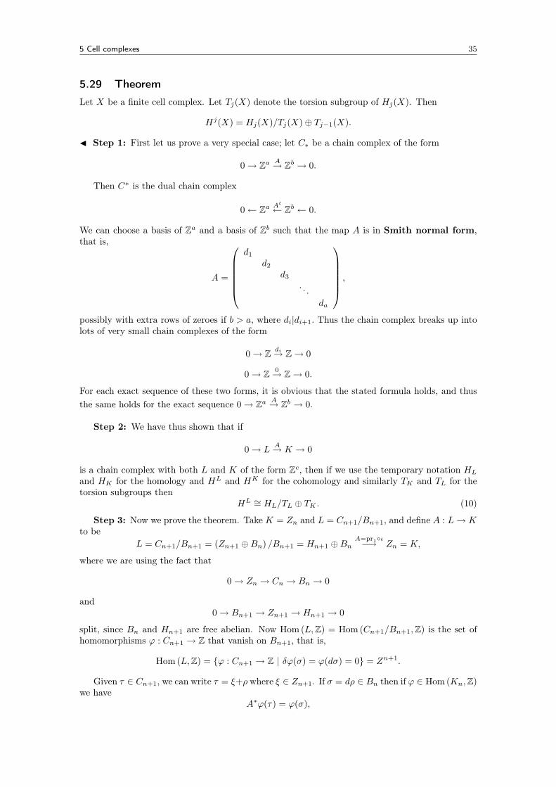
5 Cell complexes 35
5.29 TheoremLet X be a finite cell complex. Let Tj(X) denote the torsion subgroup of Hj(X). Then
Hj(X) = Hj(X)/Tj(X)⊕ Tj−1(X).
J Step 1: First let us prove a very special case; let C∗ be a chain complex of the form
0→ Za A→ Zb → 0.
Then C∗ is the dual chain complex
0← Za At← Zb ← 0.
We can choose a basis of Za and a basis of Zb such that the map A is in Smith normal form,that is,
A =
d1
d2
d3
. . .da
,
possibly with extra rows of zeroes if b > a, where di|di+1. Thus the chain complex breaks up intolots of very small chain complexes of the form
0→ Z di→ Z→ 0
0→ Z 0→ Z→ 0.
For each exact sequence of these two forms, it is obvious that the stated formula holds, and thusthe same holds for the exact sequence 0→ Za A→ Zb → 0.
Step 2: We have thus shown that if
0→ LA→ K → 0
is a chain complex with both L and K of the form Zc, then if we use the temporary notation HL
and HK for the homology and HL and HK for the cohomology and similarly TK and TL for thetorsion subgroups then
HL ∼= HL/TL ⊕ TK . (10)
Step 3: Now we prove the theorem. Take K = Zn and L = Cn+1/Bn+1, and define A : L→ Kto be
L = Cn+1/Bn+1 = (Zn+1 ⊕Bn) /Bn+1 = Hn+1 ⊕BnA=pr1ι−→ Zn = K,
where we are using the fact that
0→ Zn → Cn → Bn → 0
and0→ Bn+1 → Zn+1 → Hn+1 → 0
split, since Bn and Hn+1 are free abelian. Now Hom (L,Z) = Hom (Cn+1/Bn+1,Z) is the set ofhomomorphisms ϕ : Cn+1 → Z that vanish on Bn+1, that is,
Hom (L,Z) = ϕ : Cn+1 → Z | δϕ(σ) = ϕ(dσ) = 0 = Zn+1.
Given τ ∈ Cn+1, we can write τ = ξ+ρ where ξ ∈ Zn+1. If σ = dρ ∈ Bn then if ϕ ∈ Hom (Kn,Z)we have
A∗ϕ(τ) = ϕ(σ),

6 Generalised cohomology theories 36
and hence A∗ϕ = δϕ, that is, the image of Hom(K,Z) inside Hom(L,Z) is precisely
Bn = ψ : Cn+1 → Z | ψ = δϕ.
Thus, reverting to the old notation, we have shown
HL ∼= Hn+1(X).
Since clearlyHK∼= Hn(X)
andHL∼= Hn+1(X),
(10) yieldsHn+1(X) = Hn+1(X)/Tn+1(X)⊕ Tn(X),
which completes the proof. I
6 Generalised cohomology theories
In this chapter we define a generalised cohomology theory and look at a few examples. Webegin by defining two other cohomology theories.
6.1 Cech cohomologyLet U = Uα|α ∈ A be an open cover of X. Let
Sk (U) :=
(α0, . . . , αk) ∈ Ak+1 | Uα0 ∩ · · · ∩ Uαk 6= ∅.
LetCk(X,U) := all functions f : Sk → Z,
and define a differential δ : Ck(X,U)→ Ck+1(X,U) by
(df)(x0, . . . , xk+1) :=k∑i=0
(−1)if(x0, . . . , xi, . . . , xk).
Exactly the same proof used in for the singular complex shows that d2 = 0, and therefore we obtaina cochain complex C∗(X,U) called the Cech complex of X with respect to the open coverU. The associated cohomology is denoted H∗(X,U). For sufficiently ‘nice’ spaces X (eg. compactmanifolds) it can be shown that for ‘nice’ covers U, H∗(X,U) is actually independent of U, andthus we obtain the Cech cohomology H∗(X) of X.
Observe that H0(X) is the number of components of X, since
H0(X,U) = Z0(X,U) = f : A→ Z | Uα ∩ Uβ 6= ∅ ⇒ f(α) = f(b),
that is, H0(X,U) is the locally constant functions on X. This is in contrast to singular cohomology,where H0(X) is the number of path components of X. However, for sufficiently ‘nice’ spaces (eg.manifolds) the two concepts coincide.
6.2 Morse homologyLet M be a smooth manifold and f a ‘generic’ smooth function on M which is Morse, that is,if p ∈ M is a critical point of f (dfp = 0) than the Hessian matric Hesspf is non degenerate.Then we may write f in local coordinates locally as (x1, . . . , xd) 7→ x2
1 + · · ·+ x2j − x2
j+1− · · · − x2d.
Define CMorsek (M,f) to be the free abelian group of the critical points of f . We can then define a
differential d that ‘counts’ gradient flowlines of f . It is non-trivial result that d2 = 0, but oncethis is done, we obtain the Morse chain complex of M with respect to f . One can showthat for ‘nice’ f , the associated homology is independent of f , and hence we obtain the Morsehomology HMorse
∗ (M) of M .

6 Generalised cohomology theories 37
6.3 DefinitionsA generalised homology theory h∗ is a covariant functor from the category of pairs of spacesto the category of Z-graded abelian groups satisfying the following four axioms (we write h∗(X)for h∗(X, ∅)):
1. Homotopy: if f, g : (X,A) → (Y,B) are homotopic through maps of pairs then f∗ = g∗ asmaps h∗(X,A)→ h∗(Y,B).
2. Exactness: there exists a natural transformation, called the connecting homomorphism∂ : hn(X,A) → hn−1(A) such that if i : (A, ∅) → (X, ∅) and j : (X, ∅) → (X,A) areinclusions then
· · · → hn(A) i∗→ hn(X)j∗→ hn(X,A) ∂→ hn−1(A)→ . . .
is exact.
3. Excision: if Z ⊆ int(A) are subsets of X then the inclusion (X\Z,A\Z) → (X,A) inducesan isomorphism
h∗(X\Z,A\Z) ∼= h∗(X,A).
4. Unions: if X =⊔αXα then h∗(X) =
⊕α h∗(Xα).
Similarly one defines a generalised cohomology theory h∗ by reversing all the arrows (so h∗ isa contravariant functor) . We define a generalised reduced homology theory to be a covariantfunctor h∗ from the category of spaces to the category of Z-graded abelian groups satisfying:
1. Homotopy: if f, g : X → Y are homotopic then f∗ = g∗ as maps h∗(X)→ h∗(Y ).
2. Exactness: if A ⊆ X, there exists a natural transformation, called the connecting ho-momorphism ∂ : hn(X/A) → hn−1(A) such that if i : A → X is the inclusion map andq : X → X/A is the quotient map then
· · · → hn(A) i∗→ hn(X)q∗→ hn(X/A) ∂→ hn−1(A)→ . . .
is exact.
3. Unions: if X =⊔αXα then h∗(X) =
⊕α h∗(Xα).
6.4 Examples1. Singular cohomology: both singular homology and singular cohomology are generalised
(co)homology theories; most of Chapters 2 and 3 were devoted to verifying the axioms.Technically we haven’t yet showed that the homotopy axiom holds:
Lemma
If two maps f, g : (X,A) → (Y,B) are homotopic through maps of pairs (X,A) → (Y,B)then the induced maps f∗, g∗ : H∗(X,A) → H∗(Y,B) are equal and the induced mapf∗, g∗ : H∗ (X,A)→ H∗ (Y,B) conicide.
J The prism operator P defined in the proof of Theorem 2.17 takes Cn(A)→ Cn+1(B) andhence induces a relative prism operator P : Cn(X,A)→ Cn+1(Y,B). Then the formula ∂P +P∂ = f∗−g∗ descends to the factored complexes, and the maps f∗, g∗ : H∗ (X,A)→ H∗(Y,B)are chain homotopic, and thus induce the same homomorphism on relative homology groups,by Lemma 2.20. The proof for cohomology is similar. I
Similarly reduced singular homology and reduced singular cohomology form generalised re-duced (co)homology theories.

6 Generalised cohomology theories 38
2. Cellular cohomology: similarly, Chapter 5 was about showing that cellular cohomologysatisfied the axioms of a generalised (co)homology theory.
3. Cech cohomology: one can show that Cech cohomology satisfies the axioms of a generalisedcohomology theory.
4. Morse homology: one can also show that Morse homology satisfies the axioms of a gener-alised homology theory.
Not all generalised homology theories are obtained as the homology groups of a chain complexthough (hence the term ‘generalised’). Two examples are:
5. K-theory: to any semigroup G we can form the Grothendieck group K(G) consisting ofpairs (a, b) of elements of G subject to the rule
(a+ x, b+ x) = (a, b) for all a, b, x ∈ G
(we are meant to think of the pair (a, b) as ‘a − b’). For any space X, the set of vectorbundles over X form a semigroup, with addition E + E′ := E ⊕ E′, the Whitney sum oftwo bundles E,E′. Thus using the Grothendieck construction we obtain a group K(X). Wehave a natural map K(X)→ Z given by the rank of a bundle, and we let K0(X) denote thekernel of this map. Then for n ≥ 1, we set Kn(X) := K0(Σn(X)), where Sn(X) is the nthsuspension of X (see ). It can be shown that K∗ is then a generalised cohomology theory,which is not obtained as the cohomology of some chain complex.
6. Stabilised homotopy theory: for a space X, let
πstablen (X) := lim
k→∞πn+k(Sk(X)),
where Sk (X) is the kth suspension of X (see the proof of Corollary 4.11 for the definition ofthe suspension of a space) where πk(X) is the kth homotopy group of X. It can be shownthis forms a generalised homology theory.
For sufficently ‘nice’ spaces one hopes that all generalised cohomology theories will give isomorphiccohomology groups. Here is one important result that goes some way to satisfying this hope.
6.5 TheoremIf two generalised homology theories h∗ and k∗ are defined as the homology groups of some chaincomplex, and if h∗(pt) = k∗(pt) then they agree on everything.
Unfortunately the proof of is beyond the scope of this course. Instead we will prove the followingspecial case, which we shall use to prove the Kunneth Theorem in Chapter 7 (Theorem 7.8).
6.6 TheoremLet h∗, k∗ be generalised homology theories restricted to the category of pairs of spaces (X,A)where X is a finite cell complex and A ⊆ X a subcomplex. Suppose there exists a natural trans-formation Φ : h∗ → k∗. Then if Φ induces an isomorphism h∗(pt) ∼= k∗(pt) then Φ induces anisomorphism h∗(X,A) ∼= k∗(X,A) for all cell complexes X with subcomplexes A. Finally, the sametheorem holds with ‘generalised homology theory’ replaced with ‘generalised cohomology theory’.
J Induction of the dimension of X. If X is zero dimensional, then X is a finite union of points,and thus the union axiom and the hypotheses show h∗ and k∗ agree on (X,A).
Suppose now that the results holds for all complexes X with dimension less than or equal ton − 1, and let X be an n-dimensional cell complex. We will complete by the proof by repeatedlyusing the five lemma (Lemma 3.10).

6 Generalised cohomology theories 39
First note that by the five lemma it is enough to show that h∗(X) ∼= k∗(X), as then the middlemap in the following diagram would also be an isomorphism (by induction we already know thatΦ is an isomorphism on the other four (A has smaller dimension than X).
hm (A)i∗ //
Φ
hm (X)j∗ //
Φ
hm (X,A) ∂ //
Φ
hm−1 (A)i∗ //
Φ
hm−1 (X)
Φ
km (A)
i∗// km (X)
j∗// km (X,A)
∂// km−1 (A)
i∗// km−1 (X)
But now the five lemma again allows us to further reduce to showing that h∗(Xn, Xn−1) ∼=k∗(Xn, Xn−1):
hm+1
(Xn, Xn−1
) ∂ //
Φ
hm(Xn−1
) i∗ //
Φ
hm (Xn)j∗ //
Φ
hm(Xn, Xn−1
) ∂ //
Φ
hm−1
(Xn−1
)Φ
km+1
(Xn, Xn−1
)∂
// km(Xn−1
)i∗// km (Xn)
j∗// km
(Xn, Xn−1
)∂// km−1
(Xn−1
)Next,
h∗(Xn, Xn−1
)= h∗
(⊔α
Dnα,⊔α
∂Dnα
),
k∗(Xn, Xn−1
)= k∗
(⊔α
Dnα,⊔α
∂Dnα
),
since if we let
F :
(⊔α
Dnα,⊔α
∂Dnα
)→(Xn, Xn−1
)be a collection characteristic maps for all the n-cells of X, then by excision F∗ is an isomorphismfor both h∗ and k∗. Thus we can apply the union axiom to reduce the theorem to showingh∗(Dn, ∂Dn) ∼= k∗(Dn, ∂Dn). For this we use the fact that Dn is contractible, and hence
h∗(Dn) ∼= h∗(pt) ∼= k∗(pt) ∼= k∗(Dn),
and then apply the five lemma one more time:
hm (∂Dn)i∗ //
Φ
hm (Dn)j∗ //
Φ
hm (Dn, ∂Dn) ∂ //
Φ
hm−1 (∂Dn)i∗ //
Φ
hm−1 (Dn)
Φ
km (∂Dn)
i∗// km (Dn)
j∗// km (Dn, ∂Dn)
∂// km−1 (∂Dn)
i∗// km−1 (Dn)
This completes the proof for homology, and the proof for cohomology is similar. I
The following theorem, which we will not prove shows why singular homology is special. It isa sort of converse to the homotopy axiom.
6.7 Theorem (Whitehead)If f : X → Y is a map of spaces homotopy equivalent to cell complexes, X and Y are simplyconnected and f∗ is an isomorphism on singular homology with integer coefficients, then Xand Yare homotopy equivalent.
7 The cohomology ring 40
6.8 WarningBy parts 1 and 2 of Example 5.18 both S2×S4 and CP 3 have the same singular homology, namely
Hn
(S2 × S4
)= Hn
(CP 3
)=
Z n = 0, 2, 4, 60 n 6= 0, 2, 4, 6.
Moreover, both S2 × S4 and CP 3 are simply connected. But they are not homotopy equivalent- we will prove this in Section 10.3. Whilst they have isomorphic singular homology, there is nomap of spaces that gives rise to this isomorphism, and thus Whitehead’s theorem does not apply.
7 The cohomology ring
In this chapter we begin to explain why, in some sense, cohomology is more ‘important’ thanhomology. More precisely, we show the graded group H∗ (X) =
⊕nH
n (X) admits the structureof a graded commutative ring, the cohomology ring of X.
7.1 DefinitionLet R denote a commutative ring with unit. For cochains ϕ ∈ Ck(X;R) and ψ ∈ C`(X;R) wedefine their cup product ϕ ` ψ ∈ Ck+`(X;R) to be the cochain defined by, for σ : ∆k+` → X,
(ϕ ` ψ)(σ|[v0,...,vk+`]) = ϕ(σ|[v0,...,vk])ψ(σ|[vk,...,v`]),
where the multiplication is carried out in R. Note that ` is associative and distributive on cochains.
7.2 LemmaLet ϕ ∈ Ck(X;R) and ψ ∈ C`(X;R). Then
δ(ϕ ` ψ) = δϕ ` ψ + (−1)kϕ ` δψ. (11)
J Let σ : ∆k+`+1 → X. We have
(δϕ ` ψ)(σ|[v0,...,vk+`+1]) =k+1∑i=0
(−1)iϕ(σ|[v0,...,vi,...,vk+1])ψ(σ|[vk+1,...,vk+`+1]),
and similarly
(ϕ ` δψ)(σ|[v0,...,vk+`+1]) =k+`+1∑i−k
(−1)i+kϕ(σ|[v0,...,vk])ψ(σ|[vk,...,vi,...,vk+`+1]).
Thus in the expression(δϕ ` ψ + (−1)kϕ ` δψ
)(σ|[v0,...,vk+`+1]), the last term of the first sum
cancels the first term of the second sum, and what remains is precisely the expression for δ(ϕ `ψ)(σ|[v0,...,vk+`+1]). I
7.3 CorollaryThe cup product on cochains descends to give a product on cohomology.
J First, we must know that if ϕ ∈ Zk(X;R) and ψ ∈ Z`(X;R) then so is ϕ ` ψ, and secondlywith ϕ, ψ as above, we need to know that if
(ϕ+ δϕ′) ` (ψ + δψ′) = ϕ ` ψ + δη
for some η ∈ Ck+`−1(X;R). The first of these is immediate from (11), and for the second wecompute
(ϕ+ δϕ′) ` (ψ + δψ′) = ϕ ` ψ + δϕ′ ` ψ + ϕ ` δψ′ + δϕ′ ` δψ′
= ϕ ` ψ + δ(δϕ′ ` ψ) + (−1)kδ(ϕ ` δψ′) + δ(ϕ′ ` δψ′),
since δ2 = 0. I

7 The cohomology ring 41
7.4 LemmaIf f : X → Y then f∗ : H∗(Y ;R) → H∗(X;R) satisfies f∗(α ` β) = f∗(α) ` f∗(β). In otherwords, f∗ is a ring homomorphism on the cohomology ring (defined in Theorem 7.6).
Here and elsewhere, we will often use α and β for the cohomology class represented by ϕ andψ respectively.
J Observe that for σ : ∆k+` → X, and ϕ ∈ Ck(Y ;R), ψ ∈ C`(Y ;R), we have
(f∗(ϕ) ` f∗(ψ)) (σ|[v0,...,vk+`]) = f∗(ϕ)(σ|[v0,...,vk])f∗(ψ)(σ|[vk,...,vk+`])= ϕ(f σ|[v0,...,vk])ψ(f σ|[vk,...,vk+`])= (ϕ ` ψ)(f σ)= f∗(ϕ ` ψ)(σ).
Thus when we pass to cohomology classes the stated formula holds, since we know both f∗ and` are well defined on the level of cohomology. I
7.5 PropositionIf α ∈ Hk(X;R) and β ∈ H`(X;R) then
α ` β = (−1)k`β ` α.
J For a singular n-simplex σ : [v0, . . . , vn], let σ be the singular n-simplex obtained by precedingσ by the linear homeomorphism of [v0, . . . , vn] reversing the order of the vertices. Thus σ(vi) =σ(vn−i). Now define ρ : Cn(X)→ Cn(X) by ρ(σ) = εnσ, where
εn :=n(n+ 1)
2.
We show that ρ is a chain map that is chain homotopic to the identity. Firstly,
δρ(σ) = εn
n∑i=0
(−1)iσ|[vn,...,vn−i,...,v0],
and
ρδ(σ) = ρ
(n∑i=0
(−1)iσ|[v0,...,vi,...,vn]
)
= εn−1
n∑i=0
(−1)n−iσ|[vn,...,vn−i,...,v0].
Since εn = (−1)nεn−1, this shows ρδ = δρ.Using the subdivision of ∆n × I of Lemma 2.21, and the same notation, we now construct a
chain homotopy from ρ to the identity. Now let π : ∆n × I → ∆n denote projection, and defineP : Cn(X)→ Cn+1(X) defined by
P (σ) =n∑i=0
(−1)iεn−i(σ π|[v0,...,vi,wn,...,wi])
(so (σ π|[z0,...,zn+1]) = σ|[z0,...,zn]).In what follows, we leave out the σ and σ π for notational simplicity.Compute:
δP (σ) =∑j≤i
(−1)i(−1)jεn−i[v0, . . . , vj , . . . , vi, wn, . . . , wi]
+∑j≥i
(−1)i(−1)i+1+n−jεn−i[v0, . . . , vi, wn, . . . , wj , . . . , wi].

7 The cohomology ring 42
Next,
Pδ(σ) =∑i<j
(−1)i(−1)jεn−i−1[v0, . . . , vi, wn, . . . , wj , . . . , wi]
+∑i>j
(−1)i−1(−1)jεn−i[v0, . . . , vj , . . . , vi, wn, . . . , wi].
Since εn−i = (−1)n−iεn−i−1, the terms with i 6= j cancel in the two sums. The terms with j = iin the two terms give
εn[wn, . . . , w0]+n∑i=1
εn−i[v0, . . . , vi−1, wn, . . . , wi]+n−1∑i=0
(−1)n+i+1εn−i[v0, . . . , vi, wn, . . . , wi+1]−[v0, . . . , vn].
The two summations cancel, as replacing i by i − 1 in the second sum produces a new sign(−1)n+iεn−i+1 = −εn−i. Thus what remains is just
ε[wn, . . . , w0]− [v0, . . . , vn] = ρ(σ)− σ,
and thus δP + Pδ = ρ− 1.Now if ϕ represents α and ψ represents β, then ρ∗(ϕ) and ρ∗(ψ) also represent α and β
respectively, since ρ is chain homotopic to the identity. Now
(ρ∗(ϕ) ` ρ∗(ψ)) (σ) = ϕ(εkσ|[vk,...,v0])ψ(ε`σ|[vk+`,...,vk]),
andρ∗(ψ ` ϕ)(σ) = εk+`ψ(σ|[vk+`,...,vk])ϕ(σ|[vk,...,v0]).
Since R is assumed to be commutative, εn = (−1)nεn−1, this completes the proof. I
7.6 Theorem (the cohomology ring)Let X be a topological space and R a commutative ring with identity. Then
H∗(X;R) =⊕i
Hi(X;R)
is a graded commutative ring with identity under the cup product (that is, if α ∈ Hk(X;R)and β ∈ H`(X;R) then α ` β = (−1)k`β ` α). Moreover H∗(X;R) is an R-algebra.
J The cup product Hk(X;R)×H`(X;R)`→ Hk+`(X;R) is associative and distributive, since
it clearly is at the level of cochains. The identity element is the class 1 ∈ H0(X;R) defined bythe 0-cocycle taking the value 1 on each singular 0-simplex. Elements of H∗(X;R) are finite sums∑i αi with αi ∈ Hi(X;R), and we define the ring structure by(∑
i
αi
)`
∑j
βj
=∑i,j
αi ` βj .
This makes H∗(X;R) into a graded ring as the cup product carries Hk(X;R) × H`(X;R) intoHk+`(X;R). Graded commutativity is precisely the statement of Proposition. Taking scalarmultiplication into account, we may regard H∗(X;R) as an R-algebra. I
7.7 DefinitionGiven spaces X and Y , let πX : X × Y → X and πY : X × Y → Y denote projections. The crossproduct is the map
H∗(X;R)×H∗(Y ;R) ×→ H∗(X × Y ;R)
7 The cohomology ring 43
defined byα× β := π∗Xα ` π
∗Y β.
Since × is bilinear, it factors through the tensor product to give a linear map (also denoted ×)
H∗(X;R)⊗R H∗(Y ;R)→ H∗(X × Y ;R).
It will important in Chapter 12 (see Proposition 12.3) to observe that for α, γ ∈ H∗ (X;R) andβ, δ ∈ H∗ (Y ;R) with β ∈ Hm (X;R) and γ ∈ Hn (Y ;R) we have
(α× β) ` (γ × δ) = (π∗Xα ` π∗Y β) ` (π∗Xγ ` π
∗Y δ)
= (−1)mn π∗X (α ` γ) ` π∗Y (β ` δ) . (12)
The next theorem is an extremely important result; the clever proof we give will use Theorem6.6. It is not the sharpest theorem of this type that one can prove; in particular the assumption thatX and Y are cell complexes can be relaxed. That said, the theorem is not true in full generality,that is, (13) does not hold for arbitary spaces X and Y (an example with R = Z can be givenwhen both X and Y are real projective planes).
7.8 Theorem (Kunneth theorem)Let X and Y be cell complexes such that Hk(Y ;R) is a finitely generated free R-module for all k.Then the cross product induces an isomorphism of rings H∗(X;R)⊗RH∗(Y ;R) ×→ H∗(X×Y ;R),and thus
Hn(X × Y ;R) ∼=⊕i+j=n
Hi(X;R)⊗R Hj(Y ;R). (13)
J Consider the following functors:
hn : (X,A) 7→⊕i+j=n
Hi(X,A;R)⊗R Hj(Y ;R),
kn : (X,A) 7→ Hn(X × Y,A× Y ;R).
The aim is to apply Theorem 6.6. This means we need to show that:
1. h∗ and k∗ are generalised cohomology theories.
2. There exists a natural transformation between h∗ and k∗.
3. h∗ and k∗ agree on pt.
For the remainder of the proof we shall omit the dependence on the coefficients ‘R’ from the no-tation.
Step 1: Homotopy invariance is clear for both h∗ and k∗, that is, if f ' g than f∗ = g∗, asin both cases it follows directly from the fact that singular cohomology satisfies the axioms. Forexcision, it is immediate that h∗(X,A) ∼= h∗(B,A ∩ B) for X a cell complex with subcomplexesA,B such that X = A ∪B. For k∗, it is also clear since
(A× Y ) ∪ (B × Y ) = (A ∪B)× Y
and(A× Y ) ∩ (B × Y ) = (A ∩B)× Y,
soH∗(X × Y,A× Y ) ∼= H∗(B × Y ;A ∩B × Y ),
by excision for singular cohomology.For the long exact sequence of a pair, k∗ is immediately seen to satisfy it, and for h∗, exactness
is preserved when we tensor with H∗(Y ), since H∗(Y ) is free7. Then we obtain the desired exact7 This is where we use the fact that H∗(Y ) is free; tensoring is not in general an exact functor, but a free module
is always flat

7 The cohomology ring 44
sequence by letting i, j vary (with i + j = n), and then taking the direct sum of these exactsequences.
Finally, for unions, this again obviously holds for k∗. To check it holds for h∗, we observe thereis a canonical isomorphism (∏
α
Mα
)⊗R N ∼=
∏α
(Mα ⊗N),
for R-modules Mα and a finitely generated8 free module N .
hn
(⊕α
Xα
)=
⊕i+j=n
(Hi
(⊕α
Xα
)⊗Hj(Y )
)∼=
⊕i+j=n
⊕α
(Hi (Xα)⊗Hj(Y )
)=
⊕α
⊕i+j=n
(Hi (Xα)⊗Hj(Y )
)=
⊕α
hn (Xα) .
This completes the proof of 1.
Step 2: The cross product induces a product
H∗(X,A)⊗H∗(Y ) ×→ H∗(X × Y,A× Y ),
since if a cocycle ϕ vanishes on all simplices in A, then if ψ ∈ Z∗(Y ) is an cocycle then ϕ × ψvanishes on every simplex in A × Y . Moreover × is a natural transformation; naturality withrespect to maps between space is immediate from the naturality of cup products, and naturalitywith respect to the coboundary maps in long exact sequence is the statement that the followingdiagram commutes:
Hk (A)×H` (Y )
×
∂∗×1∗// Hk+1 (X,A)×H` (Y )
×
Hk` (A× Y )∂∗// Hk+`+1 (X × Y,A× Y )
To check this, suppose an element (α, β) in the top left-hand corner is represented by cocyclesϕ ∈ Ck(A) and ψ ∈ C`(Y ). We will show that the diagram commutes at chain level (and thuscertainly at the level of cohomology). Since ϕ ∈ Ck (A), by extending ϕ to be zero outside A weobtain an element ϕ ∈ Ck (X). Then δϕ ∈ Ck+1 (X,A), and the pair (ϕ,ψ) extends right anddown as follows
(ϕ,ψ) // (δϕ, ψ)_
π∗X (δϕ) ` π∗Y ψ.
Similarly as π∗X ϕ ` π∗Y ψ extends π∗Xϕ ` π
∗Y ψ across X × Y and
δ (π∗X ϕ ` π∗Y ψ) = π∗X (δϕ) ` π∗Y ψ,
as δψ = 0 we see that (ϕ,ψ) extends down and right as
(ϕ,ψ)_
π∗Xϕ ` π
∗Y ψ
// π∗X (δϕ) ` π∗Y ψ.
8 This is where we use the fact that H∗ (Y ) is finitely generated.
8 Interlude: categories and cup length 45
Thus the diagram commutes at chain level as claimed. This shows we have a natural transfor-mation.
Step 3: Note that if X is a point, × : hn(X)→ kn(Y ) is clearly an isomorphism, as it is justthe scalar multiplication map R⊗R Hn(Y ;R)→ Hn(Y ;R). Thus the hypotheses of Theorem 6.6are satisfied and the proof is complete. I
7.9 CorollaryLet X and Y be cell complexes. Then the Betti numbers of X × Y satisfy
bn(X × Y ) =∑i+j=n
bi(X)bi(Y ).
J Since we may compute bi(Y ) as the rank over Q asHi(Y ; Q), the conditions on Y in Theorem7.8 becomes vacuous, and then taking the ranks of both sides in 13 completes the proof. I
8 Interlude: categories and cup length
In this short chapter we take a slight break and give an application of the ring structure incohomology to smooth manifold theory.
8.1 DefinitionA category 9 is an assignment ν : 2X → N0 (where 2X denotes the power set of X andN0 = N ∪ 0) satisfying the following axioms:
• Continuity: for every A ∈ 2X there exists an open set U ⊇ A such that ν(A) = ν(U),
• Monotonicity: if A,B ∈ 2X with A ⊆ B then ν(A) ≤ ν(B),
• Subadditivity: for any A,B ∈ 2X we have ν(A ∪B) ≤ ν(A) + ν(B),
• Naturality: if ϕ : X → Y is a homeomorphism then for any A ∈ 2X , νY (ϕ(A)) = νX(A),
• Normalisation: ν(∅) = 0, and if A = x0, . . . , xn is a finite set then ν (A) = 1.
8.2 ExampleThe Ljusternik-Schirelmann category of a topological space X, written νLS, is defined as
νLS(A) := min n | there exist open contractible sets U1, . . . , Un such that A ⊆ U1 ∪ · · · ∪ Un .
Any compact manifold can be covered by finitely many sets homeomorphic to open discs, andthus if M is a compact manifold then νLS(M) < ∞ (in general, there is no reason for νLS(X) tobe finite). In fact, one can show that if M is an n-manifold then νLS(M) ≤ n + 1, although wewon’t prove this.
For any A ∈ 2SX , we have νLS(A) ≤ 2, since the suspension of any space X is covered bytwo contractible sets; namely SX = CX ∪ CX, where CX is the cone on X, and CX is alwayscontractible.
8.3 DefinitionThe cup length c`(X) of a topological space X is defined to be:
c`(X) := max n | there exist αi ∈ Hmi(X) with mi > 0 such that α1 ` · · · ` αn 6= 0 .9 Nothing to do with the ‘category’ in ‘category theory’ !

8 Interlude: categories and cup length 46
8.4 PropositionFor any space X, we have c`(X) < νLS(X).
In order to prove this we first need to introduce the relative cup product.
8.5 DefinitionThe absolute cup product restricts to a cup product Ck(X,A) × C`(X,B) → Ck+`(X,A + B),where Cn(X,A + B) is the subgroup consisting of cochains vanishes on sums of chains in A andchains in B.
We claim the inclusion Cn(X,A∪B) → Cn(X,A+B) induces an isomorphism on cohomology.Indeed, firstly, the restriction maps i∗ : Cn(A∪B)→ Cn(A+B) induces an isomorphism from theproof of Corollary 3.11. Then the five lemma shows that the desired map is indeed an isomorphism.
Cn (A ∪B) //
i∗
Cn (X) //
1∗
Cn (X,A ∪B) //
Cn+1 (A ∪B) //
i∗
Cn+1 (X)
1∗
Cn (A+B) // Cn (X) // Cn (X,A+B) // Cn+1 (A+B) // Cn (X)
Thus we can define the relative cup product on cohomology to be the map induced from thecomposition Ck(X,A)× C`(X,B)→ Ck+`(X,A+B) → Ck+`(X,A ∪B).
J Proof of Proposition 8.4: suppose νLS(X) = n, so X =⋃nj=1 Uj with each Uj con-
tractible. We claim by induction on k that if α1, . . . , αk are any cohomology classes of positivedegree then the class α1 ` · · · ` αk vanishes when restricted to H∗(U1 ∪ · · · ∪ Uk), which provesthe result. For k = 1, this is clear, as H∗(U1) = 0. Passing to the inductive step, set A :=
⋃k+1j=1 Uj ,
and consider the following commutative diagram, where U and V are any open subsets of A:
H∗ (A,U)×H∗ (A, V )
` // H∗ (A,U ∪ V )
H∗ (A)×H∗ (X)
` // H∗ (A)
In particular, if we take U =⋃kj=1 Uj , V = Uk+1, and let α = α1 ` · · · ` αk and β = αk+1,
then by induction, α ∈ H∗(A,U) and β ∈ H∗(A, V ). Thus
α ` β ∈ H∗(A,U ∪ V ) = H∗(A,A) = 0.
This proves the inductive step, and thus completes the proof. I
8.6 TheoremLet M be a smooth connected compact manifold and f : M → R a smooth function. Then f hasat least c`(M) critical points.
We will deduce this result from the following more general proposition.
8.7 PropositionLet X be a locally contractible path connected compact metric space, and φt a global flow on X.Suppose in addition there exists a Lyapunov function Φ, that is , a function Φ : X → X suchthat Φ strictly decreases along non-constant orbits of φt. Let ν : 2X → N be any category. ThenΦ has at least ν(M) critical points.

9 Cohomology of manifolds 47
J For c > 0, let Xc := Φ−1(−∞, c]. A critical value for Φ is a value such that Φ−1(c) containsa constant orbit. If c is not critical, then for sufficiently small t, δ > 0 we have
φt(Xc+δ
)⊆ Xc−δ,
since Φ strictly decreases away from the constant orbits. More generally, if c is a critical level andU is any neighborhood of Φ−1 (c) then for small t, δ > 0
we haveφt(Xc+δ\U
)⊆ Xc−δ. (14)
For j = 1, . . . , N := ν(X), letcj := supc | ν(Xc) < j.
Then c1 = minΦ (as ν(pt) = 1) and cN = maxΦ. Note that cj is a critical value of Φ for eachj.
We claim that either cj < cj+1 or Φ−1(cj) contains infinitely many critical points. Suppose thelatter doesn’t happen, with say Φ−1 (cj) = x0, . . . , xn. Then by the normalisation axiom theeexists a neighborhood U of x0, . . . , xn such that ν (U) = 1.
Then by (14) and the monotonicity and naturality axioms, for sufficiently small δ > 0 we have
ν(Xcj+δ
)≤ ν
(Xcj+δ\U
)+ 1,
≤ ν(Xcj−δ
)+ 1
≤ j + 1,
implying cj+1 ≥ cj + δ > cj . Thus either we can find infinitely many critical points, in which casethe theorem is trivially true, or c1 < · · · < cN , and thus we have at least N = ν(X) critical points.This completes the proof. I
J Proof of Theorem 8.6: giveM a Riemannian metric 〈·, ·〉 and let ∇f denote the gradientof f with respect to 〈·, ·〉, that is, the unique vector field defined by
〈(∇f)p, Xp〉 = dfp (Xp)
for every vector field X on M . Note that the critical points of f are precisely the zeros of ∇f .Let φt denote the associated flow of ∇f , which is defined for all t ∈ R by compactness of M .
We claim that f itself is a Lyapunov function for φt. To see this, let cp be the curve in M definedby cp (t) = φt (p), then
d
dt(f cp (t)) = df (cp (t))
=⟨(∇f)cp(t), cp(t)
⟩= −〈cp(t), cp(t)〉 ≤ 0,
with equality if and only if cp(t) = 0, that is, p is a critical point of f , and so cp (t) ≡ p for all t.Thus all the conditions of Proposition 8.7 are satisfied, and thus Proposition 8.4 completes the
proof. I
9 Cohomology of manifolds
In this chapter we introduce cohomology with compact support, and use this to computethe top dimensional cohomology of closed manifolds (where ‘closed’ means compact and withoutboundary), namely: let Mn be a closed connected manifold. Then
Hn (M) ∼=
Z if M is orientable,Z2 if M is not orientable
(15)
(this is Theorem 9.15). In the next chapter we will use this to prove the most important theoremwe will meet in the course, Poincaré duality.
9 Cohomology of manifolds 48
9.1 DefinitionA topological manifold Mn is said to be of type k if it admits an open cover M =
⋃ki=1Oi, such
that there exist homeomorphisms hi : Oi ∼= Rn (we call such a set Oi an open disc in M), suchthat all possible intersections ⋂
j∈JOj , J ⊆ 1, . . . , k,
are empty or also homeomorphic to a disjoint collection of open discs in M , and k is minimal withthis property.
If M has type k for some k then M is said to be of finite type. If M is compact it can beshown that M has finite type10.
The argument we will use to prove Theorem 9.15 later will involve induction on type; thisis an extremely powerful method that we will use to prove Poincaré duality in the next chapter.Unfortunately the cohomology theory we have developed so far is poorly suited to this task, as amanifold M with type 1 (the base case of the induction step) is homeomorphic to Rn and hence(15) is false for M . What we will therefore do is develop an alternative cohomology H∗ct such thatH∗ct (M) = H∗ (M) for M compact, and
Hmct (Rn) =
Z m = n,
0 m 6= n.(16)
9.2 DefinitionLetX be a topological space. The cochain complex of singular cochains with compact supportis defined as
Cmct (X) :=ϕ ∈ Cm(X) | there exists a compact set K = K(ϕ) ⊆ X such that ϕ|X\K ≡ 0
.
The usual differential operator δ on C∗(X) preserves C∗ct(X), as if ϕ vanishes on X\K then sodoes δϕ: if σ : ∆m+1 → X has im σ ⊆ X\K then clearly all its faces are also contained in X\K.Thus this does indeed define a chain complex under the standard differential. The associatedcohomology is called the singular cohomology with compact supports, written H∗ct(X).
Observe that if X is compact then C∗ct(X) = C∗(X), as any cochain vanishes on the empty set(i.e. we may take K = X), and hence H∗ct (X) = H∗ (X).
The definition of Cmct (X) seems slightly contrived; it would be more natural perhaps to requireϕ ∈ Ck(X) to be compactly supported as a function11. Unfortunately then δ would not thenpreserve C∗ct (X): consider ϕ ∈ C0(R) that is non-zero only at the origin. Then ϕ is compactlysupported but δϕ|[0,N ] is non-zero for any N ∈ N, and thus δϕ is not compactly supported as afunction.
Although this definition is intuitive, it is not easy to compute with. We will generally work witha more algebraic definition. In order to introduce this, we need some more technical machinery.
9.3 DefinitionsA directed system of abelian groups Ga | a ∈ A is a collection of abelian groups indexed by apartially ordered set A satisfying:
• For all a, b ∈ A there exists c ∈ A such that a < c and b < c.
• For all a ≤ b there exists a homomorphism ρab : Ga → Gb such that ρaa = id and if a ≤ b ≤ c,ρbc ρab = ρac.
10 In the smooth case this can be easily seen by covering M with sufficiently small geodesic balls, as then allintersections are then geodesically convex, and thus homeomorphic to open discs.
11 Which is what is required in the de Rham compactly supported cohomology.

9 Cohomology of manifolds 49
The direct limit lim−→Ga is defined to be
lim−→a∈A
Ga :=⊔a∈A
Ga/ ∼,
where x ∼ y if x ∈ Ga, y ∈ Gb and there exists c such that ρac(x) = ρbc(y) (note that ∼ is anequivalence relation; this is why we need the Ga to be abelian); equivalently we could take ∼ tobe the equivalence relation defined by x ∼ ρab(x). This gives us another definition:
lim−→a∈A
Ga :=⊕a∈A
Ga/H,
where H := 〈x− ρab(x) | x ∈ Ga〉, where we consider Ga as a subgroup of⊕
a∈AGa under thenatural inclusion.
Next, lim−→Ga is a group, with addition defined as follows. Given classes [x], [y], pick a representa-tive x ∈ Ga, say and y ∈ Gb. Choose c such that a < c, b < c and then set x′ = ρac(x), y′ = ρbc(y).Then we may form x′ + y′ ∈ Gc, and we define [x] + [y] to be the class representated by x′ + y′,that is, [x] + [y] := [x′ + y′].
We can also consider directed systems of chain complexes; we will do this in Lemma 9.14, below.
9.4 LemmaIf Ga | a ∈ A is a directed system of abelian groups, and A′ ⊆ A is a subset with the propertythat for all a ∈ A there exists b ∈ A′ such that a ≤ b then
lim−→a∈A
Ga = lim−→a∈A′
Ga.
In particular, if A has a maximal element α then
lim−→a∈A
Ga = Gα.
J Immediate from the definition of lim−→Ga. I
9.5 DefinitionThe alternative definition for H∗ct(X) defines it directly, rather than as the cohomology of somecochain complex.
For a space X, the compact subsets K ⊆ X form a directed system under inclusion since theunion of two compact sets is compact. Moreover, if K1 ⊆ K2 then X\K2 ⊆ X\K1 and thusthe inclusion (X,X\K2) → (X,X\K1) induces a pullback homomorphism ρ12 : Hm(X|K1) →Hm(X|K2), (recall the notation Hm (X|K) := Hm (X,X\K))and hence we may define the directlimit:
Hmct (X) := lim−→
K⊆X compactordered by inclusion
Hm(X|K).
To see that the definitions are equivalent, observe that an element of lim−→Hm(X,X\K) is
represented by a cocycle in Cm(X,X\K) for some compact K, and such a cocycle is zero inlim−→H
k(X,X\K) if and only if it is the coboundary of a cochain in Cm−1(X,X\L) for some com-pact L ⊇ K.

9 Cohomology of manifolds 50
9.6 ExampleWe compute H∗ct(Rn). By Lemma 9.4, since every compact set of Rn is contained in the closedball DR(0) for some R ∈ N, it is enough to take the limit over such discs:
Hmct (Rn) = lim−→
R∈NHm (Rn|DR(0)) .
Now observe that for any R > 0,
Hm (Rn|DR(0)) =
Z m = n
0 m 6= n,
as Rn\DR(0) is homotopy equivalent to Sn−1, and thus the long exact sequence for the pair(Rn,Rn\DR(0)) is (for n ≥ 1 )
· · · → Hm(Rn)→ Hm (Rn|DR(0))→ Hm+1(Sn−1)→ Hm+1(Rn)→ . . .
Moreover, the mapsHn (Rn|DR(0))→ Hn (Rn|DR+1(0)) corresponding to the inclusions (Rn,Rn\DR+1(0)) →(Rn,Rn\DR(0)) are isomorphisms, since the two spaces are clearly homotopy equivalent. We con-clude that
Hmct (Rn) =
Z m = n
0 m 6= n,
which agrees with what we wanted in (16)
9.7 WarningUnfortunately there is a major price to pay. Singular cohomology with compact supports is nota cohomology theory! It is not a homotopy invariant; a point is compact so H∗ct(pt) is equal toH∗(pt), but as we have just seen H∗ct(Rn) is not equal to H∗(Rn). It is not even a functor - theconstant map Rn → pt does not induce a map H∗ct(pt)→ H∗ct(Rn).
However if we restrict to proper maps, that is, closed maps f whose preimages of compact setsare compact then there is a pullback map f∗ on H∗ct, since if f : X → Y is proper .and ϕ ∈ Ck(Y )vanishes on the complement of the compact set K ⊆ Y then f∗ (ϕ) vanishes on the complementof the compact set f−1(K) ⊆ X.newline
Thus restricting to the category of topological spaces and proper maps, we can make H∗ct intoa contravariant functor, just as we did with H∗ct. However what we will actually do is make H∗ctinto a covariant functor, using the following construction.
9.8 Extension by zeroLet i : U → X be inclusion of an open set U ⊆ X, or more generallly, let i : U → X bea homeomorphism onto an open subset i(U) ⊆ X. We will show that i induces a map called‘extension by zero’, a pushforward map i∗ : H∗ct(U)→ H∗ct(X). We will give two definitions, onecorresponding to each of our definitions of H∗ct; as before the first is intuitive, but would requirework to show that it really is independent of the choices made, and thus we will in general use thesecond.
Here is the first definition. Suppose ϕ ∈ Ckct(U) vanishes on the complement of the compactset K ⊆ U . Take a k-chain σ ∈ Ck(X). Subdivide σ (eg. barycentrically) into smaller chains σisuch that each is either disjoint from K or wholly contained in U . Define
i∗(ϕ)(σ) =∑σi⊆U
ϕ(σi);
note that i∗(σ) still vanishes on the complement of K, which is still compact as a subset of X, andhence i∗(ϕ) ∈ Ckct(X). This induces a map i∗ : H∗ct(U)→ H∗ct(X).
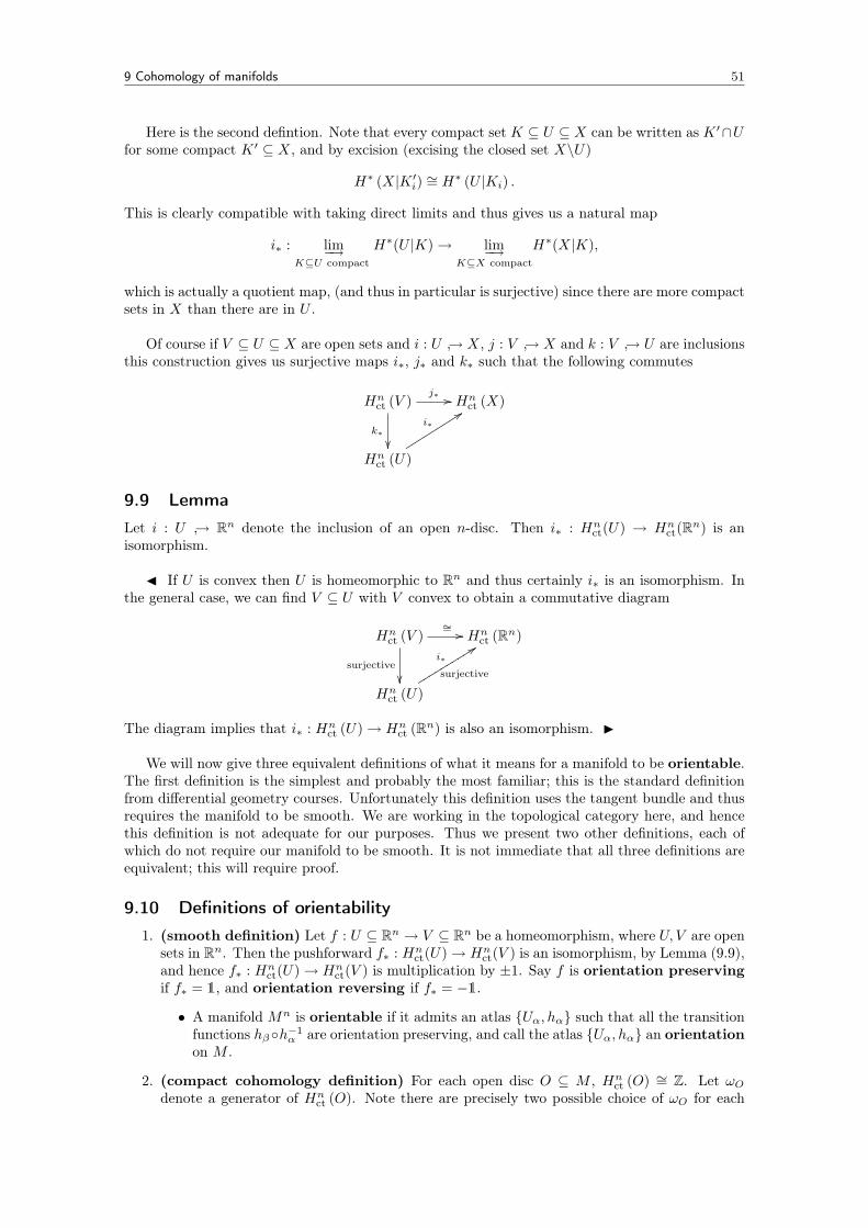
9 Cohomology of manifolds 51
Here is the second defintion. Note that every compact set K ⊆ U ⊆ X can be written as K ′∩Ufor some compact K ′ ⊆ X, and by excision (excising the closed set X\U)
H∗ (X|K ′i) ∼= H∗ (U |Ki) .
This is clearly compatible with taking direct limits and thus gives us a natural map
i∗ : lim−→K⊆U compact
H∗(U |K)→ lim−→K⊆X compact
H∗(X|K),
which is actually a quotient map, (and thus in particular is surjective) since there are more compactsets in X than there are in U .
Of course if V ⊆ U ⊆ X are open sets and i : U → X, j : V → X and k : V → U are inclusionsthis construction gives us surjective maps i∗, j∗ and k∗ such that the following commutes
Hnct (V )
k∗
j∗ // Hnct (X)
Hnct (U)
i∗
99sssssssss
9.9 LemmaLet i : U → Rn denote the inclusion of an open n-disc. Then i∗ : Hn
ct(U) → Hnct(Rn) is an
isomorphism.
J If U is convex then U is homeomorphic to Rn and thus certainly i∗ is an isomorphism. Inthe general case, we can find V ⊆ U with V convex to obtain a commutative diagram
Hnct (V )
surjective
∼= // Hnct (Rn)
Hnct (U)
surjective
i∗
99ssssssssss
The diagram implies that i∗ : Hnct (U)→ Hn
ct (Rn) is also an isomorphism. I
We will now give three equivalent definitions of what it means for a manifold to be orientable.The first definition is the simplest and probably the most familiar; this is the standard definitionfrom differential geometry courses. Unfortunately this definition uses the tangent bundle and thusrequires the manifold to be smooth. We are working in the topological category here, and hencethis definition is not adequate for our purposes. Thus we present two other definitions, each ofwhich do not require our manifold to be smooth. It is not immediate that all three definitions areequivalent; this will require proof.
9.10 Definitions of orientability1. (smooth definition) Let f : U ⊆ Rn → V ⊆ Rn be a homeomorphism, where U, V are open
sets in Rn. Then the pushforward f∗ : Hnct(U)→ Hn
ct(V ) is an isomorphism, by Lemma (9.9),and hence f∗ : Hn
ct(U)→ Hnct(V ) is multiplication by ±1. Say f is orientation preserving
if f∗ = 1, and orientation reversing if f∗ = −1.
• A manifold Mn is orientable if it admits an atlas Uα, hα such that all the transitionfunctions hβ h−1
α are orientation preserving, and call the atlas Uα, hα an orientationon M .
2. (compact cohomology definition) For each open disc O ⊆ M , Hnct (O) ∼= Z. Let ωO
denote a generator of Hnct (O). Note there are precisely two possible choice of ωO for each

9 Cohomology of manifolds 52
open disc O. Let ωOO⊆M denote a choice of generators for each open disc O. Given opendiscs O ⊆ O′ and i : O → O′ the inclusion, we have an isomorphism i∗ : Hn
ct (O)→ Hnct (O′)
which must carry ωO to a generator.
• A manifold Mn is orientable if we can choose ωOO⊆M satisfying the compatibiltycondition that given O ⊆ O′ as above we have
i∗ (ωO) = ωO′ ,
and call the collection ωOO⊆M an orientation on M .
3. (homology definition) Define an a local orientation of a point x ∈Mn to be a generatorof µx ∈ Hn (M |x). Note there are precisely two possible local orientations at x. Let µxx∈Mdenote a choice of generators for each x ∈ M . Suppose h : U → Ω ⊆ Rn is a chart about x.By excision for any y ∈ U we have an isomorphism
φ : Hn (M |x) ∼= Hn (Rn|h(x)) ∼= Hn (Rn|Ω) ∼= Hn (Rn|h (y)) ∼= Hn (M |y) ,
which must carry µx to a generator of Hn (M |y).
• A manifold Mn is orientable if we can choose µxx∈M such that given x and y in thedomain of a chart as above we have
φ (µx) = µy,
and call the collection µxx∈M an orientation on M .
It follows straight from the definitions that in the smooth case the first two conditions are equiv-alent. The equivalence of the second and third definitions is somewhat harder, and we will omitthe proof of this. Instead, we prove the following theorem, which we shall need in Chapter 9 inorder to define the fundamental class of a closed manifold (see Definition 10.11), as well as inthe proof of Poincaré duality.
9.11 TheoremIf M is oriented with orientation µxx∈M then for each K ⊆ M compact there exists a uniqueelement µK ∈ Hn(M |K) such that for all x ∈ K, the inclusion jx : M\K → M\x induces amap jx∗ : Hn(M |K)→ Hn(M |x) such that jx∗(µK) = µx. Moreover Hi (M |K) = 0 for i > n.
J The proof proceeds in three steps.newlineStep 1: Suppose the result holds for compact subsets A, B and A ∩ B of M . We show this
implies it holds for the compact set A ∪B. Consider the Mayer-Vietoris sequence
0 = Hn+1 (M |A ∩B)→ Hn (M |A ∪B)→ Hn (M |A)⊕Hn (M |B)ψ→ Hn (M |A ∩B)→ . . .
By induction we easily see Hn+1 (M |A ∪B) = 0. Moreover existence of µA and µB , and unique-ness of µA∩B implies µA|A∩B = µB |A∩B , and thus (µA, µB) ∈ kerψ. Thus there exists a necessarilyunique element µA∪B mapping onto (µA, µB) by exactness, and we easily see that µA∪B satisfiesthe required conditions.
Step 2: Now suppose K ⊆M is compact. Write K = K1∪· · ·∪Kr where each Ki is containedin an open disc Oi. Suppose by induction that the result holds for unions of at most r − 1 suchsets. Then it holds for K1 ∪ · · · ∪Kr−1 and Kr, and hence by Step 1, K1 ∪ · · · ∪Kr. Thus we havereduced the proof to the case r = 1, that is, K ⊆ O ⊆M where O is an open disc, or equivalently,K ⊆ Rn.
Then observe that if K ⊆ Rn happened to be convex, since then Hn (Rn|K) ∼= Hn (Rn|0) byhomotopy invariance, and it easily follows the theorem holds for K. Moreover if K ⊆ Rn can bewritten as a finite union of convex sets then by induction and Step 1 again, we see the theoremholds for K.
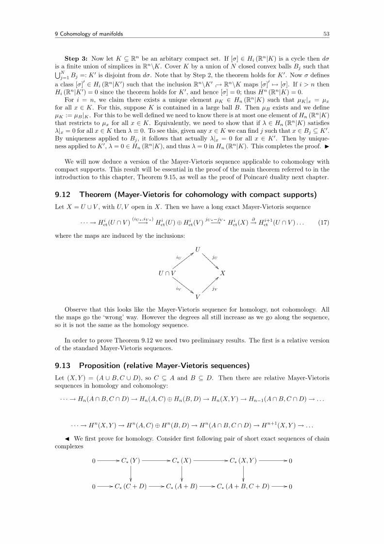
9 Cohomology of manifolds 53
Step 3: Now let K ⊆ Rn be an arbitary compact set. If [σ] ∈ Hi (Rn|K) is a cycle then dσis a finite union of simplices in Rn\K. Cover K by a union of N closed convex balls Bj such that⋃Nj=1Bj =: K ′ is disjoint from dσ. Note that by Step 2, the theorem holds for K ′. Now σ defines
a class [σ]′ ∈ Hi (Rn|K ′) such that the inclusion Rn\K ′ → Rn\K maps [σ]′ 7→ [σ]. If i > n thenHi (Rn|K ′) = 0 since the theorem holds for K ′, and hence [σ] = 0; thus Hn (Rn|K) = 0.
For i = n, we claim there exists a unique element µK ∈ Hn (Rn|K) such that µK |x = µxfor all x ∈ K. For this, suppose K is contained in a large ball B. Then µB exists and we defineµK := µB |K . For this to be well defined we need to know there is at most one element ofHn (Rn|K)that restricts to µx for all x ∈ K. Equivalently, we need to show that if λ ∈ Hn (Rn|K) satisfiesλ|x = 0 for all x ∈ K then λ ≡ 0. To see this, given any x ∈ K we can find j such that x ∈ Bj ⊆ K ′.By uniqueness applied to Bj , it follows that actually λ|x = 0 for all x ∈ K ′. Then by unique-ness applied toK ′, λ = 0 ∈ Hn (Rn|K), and thus λ = 0 inHn (Rn|K). This completes the proof. I
We will now deduce a version of the Mayer-Vietoris sequence applicable to cohomology withcompact supports. This result will be essential in the proof of the main theorem referred to in theintroduction to this chapter, Theorem 9.15, as well as the proof of Poincaré duality next chapter.
9.12 Theorem (Mayer-Vietoris for cohomology with compact supports)Let X = U ∪ V , with U, V open in X. Then we have a long exact Mayer-Vietoris sequence
· · · → Hict(U ∩ V )
(iU∗,iV ∗)−→ Hict(U)⊕Hi
ct(V )jU∗−jV ∗−→ Hi
ct(X) ∂→ Hi+1ct (U ∩ V ) . . . (17)
where the maps are induced by the inclusions:
UjU
@@@@@@@@
U ∩ V
iV ##FFFFFFFFF
iU
;;xxxxxxxxxX
V
jV
>>~~~~~~~
Observe that this looks like the Mayer-Vietoris sequence for homology, not cohomology. Allthe maps go the ‘wrong’ way. However the degrees all still increase as we go along the sequence,so it is not the same as the homology sequence.
In order to prove Theorem 9.12 we need two preliminary results. The first is a relative versionof the standard Mayer-Vietoris sequences.
9.13 Proposition (relative Mayer-Vietoris sequences)Let (X,Y ) = (A ∪ B,C ∪ D), so C ⊆ A and B ⊆ D. Then there are relative Mayer-Vietorissequences in homology and cohomology:
· · · → Hn(A ∩B,C ∩D)→ Hn(A,C)⊕Hn(B,D)→ Hn(X,Y )→ Hn−1(A ∩B,C ∩D)→ . . .
· · · → Hn(X,Y )→ Hn(A,C)⊕Hn(B,D)→ Hn(A ∩B,C ∩D)→ Hn+1(X,Y )→ . . .
J We first prove for homology. Consider first following pair of short exact sequences of chaincomplexes
0 // C∗ (Y ) //
C∗ (X) //
C∗ (X,Y ) //
0
0 // C∗ (C +D) // C∗ (A+B) // C∗ (A+B,C +D) // 0

9 Cohomology of manifolds 54
Here Cn(A + B,C + D) is defined as the quotient of the subgroup Cn(A + B) by its subgroupCn(C + D), and hence the second sequence is exact. The vertical maps are restrictions. Thefirst and second and of these induce isomorphisms on homology, as the argument in the proof ofTheorem 3.5 shows. Thus passing to the associated long exact sequence and applying the fivelemma the first vertical map also induces isomorphisms on homology.
Now consider the following commutative diagram:
0
0
0
0 // Cn (C ∩D)
φ // Cn (C)⊕ Cn (D)
ψ // Cn (C +D)
// 0
0 // Cn (A ∩B)
φ // Cn (A)⊕ Cn (B)
ψ // Cn (A+B)
// 0
0 // Cn (A ∩B,C ∩D)
φ // Cn (A,C)⊕ Cn (B,D)
ψ // Cn (A+B,C +D)
// 0
0 0 0
The three columns are exact, and from standard Mayer-Vietoris the first two rows are exact.We claim the third row is also exact, where the maps φ, ψ are those induced from the second row.Indeed, since ψ φ = 0 in the second row, this also holds in the third row, and hence the third rowis a chain complex. Now consider the whole diagram as a short exact sequence of chain complexes,as in Definition 3.1. Since the first two rows are exact, the associated long exact sequence inhomology of this short exact sequence of chain complexes has two out of every three terms zero.But then every term is zero, and thus the third row is also exact.
Thus we may take the long exact sequence of the short exact sequence
0→ C∗(A ∩B,C ∩D)→ C∗(A,C)⊕ C∗(B,D)→ C∗(A+B,C +D)→ 0, (18)
and then finally use the isomorphism H∗(A+B,C +D) ∼= H∗(X,Y ) mentioned at the beginningof the proof to obtain the desired sequence. This completes the proof for homology.
For cohomology, first consider the following pair of short exact sequences of cochain complexes:
0 // C∗ (X,Y ) //
C∗ (X) //
C∗ (Y ) //
0
0 // C∗ (A+B,C +D) // C∗ (A+B) // C∗ (C +D) // 0
Here Cn(A + B,C + D) is defined as the kernel of Cn(A + B) → Cn(C + D), the restrictionmap, so the second sequence is exact. The vertical maps are restrictions. The second and thirdof these induce isomorphisms on cohomology, as the argument in given in the proof of Corollary3.11hows. Thus passing to the associated long exact sequence and applying the five lemma thefirst vertical map also induces isomorphisms on cohomology.
The relative sequence we are after is then the long exact sequence associated to the short exactsequence of cochain complexes
0→ C∗(A+B,C +D)→ C∗(A,C)⊕ Cn(B,D)→ C∗(A ∩B,C ∩D)→ 0.
This is exact since it is the dual of the short exact sequence in equation 18, and taking the dualyields an exact sequence as Cn(A+ B,C +D) is free, with basis the singular n-simplices in A orB that do not lie in C or D. I
Then next thing is prove that the direct limit functor is exact.

9 Cohomology of manifolds 55
9.14 LemmaLet Cα, fαβ | α, β ∈ Γ be a directed system of chain complexes, with maps fαβ : Cα → Cβ chainmaps. Then
Hn
(lim−→Cα
)= lim−→Hn(Cα).
J We will first prove a more general exactness prinicple: let Aα, Bα, Cα be directedsystems for α ∈ Γ, where Γ is a directed set such that we have sequences
Aαfα→ Bα
gα→ Cα
which are exact at Bα. Let A := lim−→Aα, B := lim−→Bα and C := lim−→Cα. We will write iαβ : Aα → Aβfor the maps for α < β, and use the same symbol for the maps Bα → Bβ , Cα → Cβ (this will notcause confusion). The maps fα induce a map f : A→ B, obtained by thinking of an element ofA as the image of an element of
⊕α∈ΓAα. We will prove that
Af→ B
g→ C
is exact.It is clear that gf = 0. Suppose g(b) = 0. Choose an element b′ ∈
⊕αBα whose image is b.
Then b′ = bα1 + · · ·+ bαn for some bαi ∈ Bαi , since elements of the direct sum⊕
αBα have onlyfinitely many non-zero terms. Since Γ is directed, there exists β ∈ Γ such that αi < β for eachi = 1, . . . , n. Then the element
b′′ =n∑i=1
iαiβ(bαi) ∈ Bβ
has the same image as b′ in B, namely b. Now g(b) is the image of gβ(b′′) ∈ Cβ ⊆⊕
α Cα. Sinceg(b) = 0, there exists γ > β such that iβγ(g(b′′)) = 0. Now consider b′′′ := iβγ(b′′) ∈ Bγ . Thengγ(b′′′) = 0, so there exists a′ ∈ Aγ such that fγ(a′) = b′′′. Then let a denote the image in A of a′.Then f(a) = b, and this proves the exactness prinicple.
Now we can prove the lemma itself. Write (Cn)α for the nth group of the chain complex Cα.We want to show
Hm
(lim−→α(Cn)α
)= lim−→αHm
(lim−→α(Cn)α
)for each m ∈ Z. Consider first the sequence
0→ (Zn)α → (Cn)α(dn)α→ (Cn−1)α,
where (Zn)α is the kernel of the differential (dn)α of Cα. This is exact at (Zn)α and (Cn)α. Takingthe direct limit and using the exactness principle above, we deduce the following is exact:
0→ lim−→α(Zn)α → lim−→α(Cn)αdn→ lim−→α(Cn−1)α,
where dn is the map obtained from the (dn)α. Thus the kernel of dn is lim−→α(Zn)α. Now we repeatfor boundaries, using
0→ (Zn+1)α → (Cn+1)α(dn+1)α→ (Bn)α → 0
to obtain with the obvious notation
lim−→α(Zn+1)α → lim−→α(Cn+1)αdn+1→ lim−→α(Bn)α → 0.
Thus since dn+1 is surjective, and lim−→α(Zn+1)α is the kernel of dn+1, we deduce that the image ofdn+1is lim−→α(Bn)α.
Finally, we use the short exact sequence defining homology:
0→ (Bn)α → (Zn)α → (Hn)α → 0.
Taking direct limits gives
0→ lim−→α(Bn)α → lim−→α(Zn)α → lim−→α(Hn)α → 0,
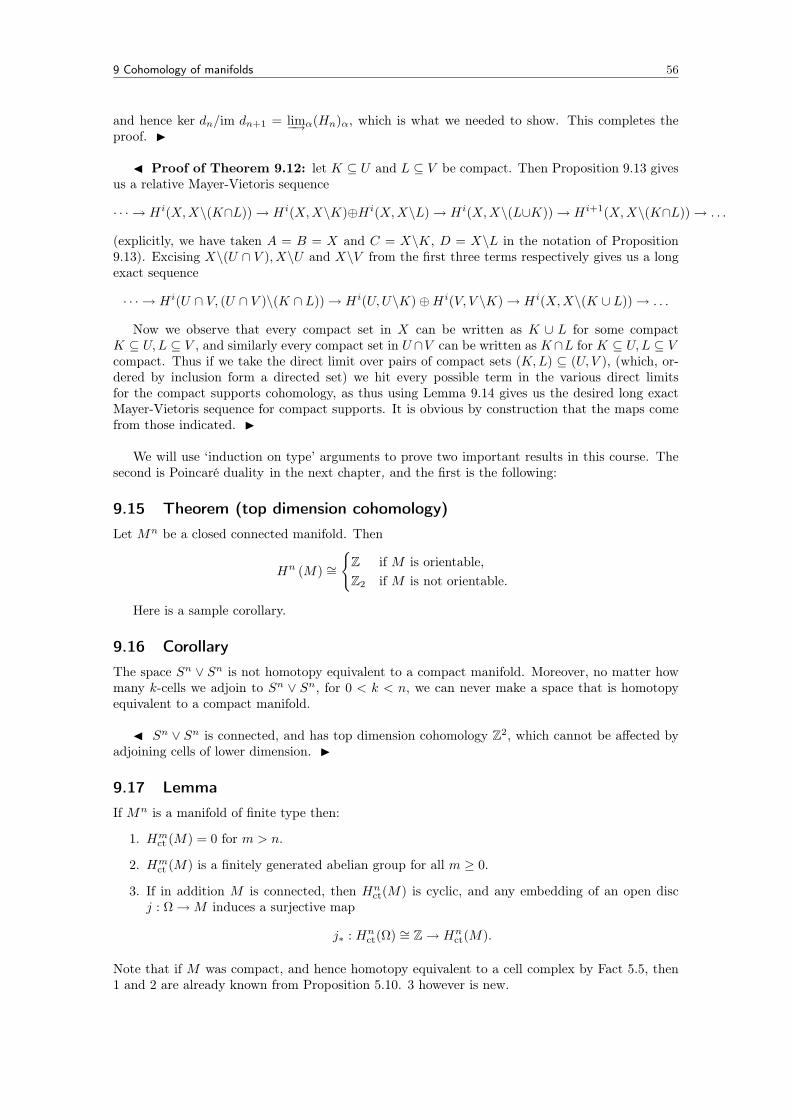
9 Cohomology of manifolds 56
and hence ker dn/im dn+1 = lim−→α(Hn)α, which is what we needed to show. This completes theproof. I
J Proof of Theorem 9.12: let K ⊆ U and L ⊆ V be compact. Then Proposition 9.13 givesus a relative Mayer-Vietoris sequence
· · · → Hi(X,X\(K∩L))→ Hi(X,X\K)⊕Hi(X,X\L)→ Hi(X,X\(L∪K))→ Hi+1(X,X\(K∩L))→ . . .
(explicitly, we have taken A = B = X and C = X\K, D = X\L in the notation of Proposition9.13). Excising X\(U ∩ V ), X\U and X\V from the first three terms respectively gives us a longexact sequence
· · · → Hi(U ∩ V, (U ∩ V )\(K ∩ L))→ Hi(U,U\K)⊕Hi(V, V \K)→ Hi(X,X\(K ∪ L))→ . . .
Now we observe that every compact set in X can be written as K ∪ L for some compactK ⊆ U,L ⊆ V , and similarly every compact set in U ∩V can be written as K∩L for K ⊆ U,L ⊆ Vcompact. Thus if we take the direct limit over pairs of compact sets (K,L) ⊆ (U, V ), (which, or-dered by inclusion form a directed set) we hit every possible term in the various direct limitsfor the compact supports cohomology, as thus using Lemma 9.14 gives us the desired long exactMayer-Vietoris sequence for compact supports. It is obvious by construction that the maps comefrom those indicated. I
We will use ‘induction on type’ arguments to prove two important results in this course. Thesecond is Poincaré duality in the next chapter, and the first is the following:
9.15 Theorem (top dimension cohomology)Let Mn be a closed connected manifold. Then
Hn (M) ∼=
Z if M is orientable,Z2 if M is not orientable.
Here is a sample corollary.
9.16 CorollaryThe space Sn ∨ Sn is not homotopy equivalent to a compact manifold. Moreover, no matter howmany k-cells we adjoin to Sn ∨ Sn, for 0 < k < n, we can never make a space that is homotopyequivalent to a compact manifold.
J Sn ∨ Sn is connected, and has top dimension cohomology Z2, which cannot be affected byadjoining cells of lower dimension. I
9.17 LemmaIf Mn is a manifold of finite type then:
1. Hmct (M) = 0 for m > n.
2. Hmct (M) is a finitely generated abelian group for all m ≥ 0.
3. If in addition M is connected, then Hnct(M) is cyclic, and any embedding of an open disc
j : Ω→M induces a surjective map
j∗ : Hnct(Ω) ∼= Z→ Hn
ct(M).
Note that if M was compact, and hence homotopy equivalent to a cell complex by Fact 5.5, then1 and 2 are already known from Proposition 5.10. 3 however is new.

9 Cohomology of manifolds 57
J We will induct on the type k. The case k = 1 is M ∼= Rn, and all three parts were provedin Example 9.6. We pass therefore to the inductive step. Write M = O ∪N , where O is an opendisc in M , and both N and U := O ∩N have type strictly less than k.
Let the inclusions iO, iN , jO, jN be as pictured:
OjO
BBBBBBBB
U
iN @@@@@@@
iO
>>~~~~~~~M
N
jN
>>
1 is then immediate from the Mayer-Vietoris sequence. 2 is equally easy, since Hmct (M) is
flanked by finitely generated abelian groups (by induction) in the exact sequence (17), and becauseof the two algebraic facts that if H ≤ G and G/H are finitely generated so is G, and any subgroupof a finitely generated abelian group is also a finitely generated abelian group.
It therefore remains to prove 3. Since in this case M is assumed connected, we must haveU 6= ∅. Thus we may embed an open disc i : Ω → U , and following it with the inclusion gives amap
i : Ω→ U → O ∼= Rn.
The induced map i∗ : Hnct (Ω) → Hn
ct (O) is an isomorphism by Lemma 9.9. This shows thatthe map iO∗ : Hn
ct(U) → Hnct(O) is surjective - it is not necessarily an isomorphism as U is not
necessarily connected; however if U is connected then this map is an isomorphism (this will beimportant in Proposition 9.18 below). The sequence (17) is
· · · → Hnct(U)
ψ→ Hnct(O)⊕Hn
ct(N)ϕ→ Hn
ct(M)→ 0,
where ϕ is surjective by 1. Thus if c ∈ Hnct(M), by exactness, there exists (m, c1) ∈ Hn
ct(O)⊕Hnct(N)
such that ϕ(m, c1) = c. Since iO∗ is surjective, there exists u ∈ Hnct(U) such that ψ(u) = (m, c2)
for some c2 ∈ Hnct(N). Thus c = ϕ(0, c1 − c2), since ϕ(m, c2) = ϕψ(u) = 0. This shows that
jN : Hnct(N)→ Hn
ct(M) is surjective.Now by induction, Hn
ct(N) is cyclic, and thus Hnct(M) is the quotient of a cyclic group, and
hence is cyclic. For the final statement of 3, if j : Ω → M is an open disc then either Ω ∩ O 6= ∅or Ω ∩ N 6= ∅; without loss of generality assume the latter. Then Ω ∩ N is an open disc in M ;by induction and the computations above in the diagram below the bottom map and the two sideones surject:
Hnct (Ω)
j∗ // Hnct (M)
Hnct (Ω ∩N) //
OO
Hnct (N)
OO
Hence so does j∗. This completes the proof. I
We can now prove the first half of Theorem 9.15.
9.18 PropositionLet Mn be an oriented manifold of finite type.
1. There is a unique map∫M
: Hnct(M)→ Z such that
∫Mi∗ (ωO) = 1 for each embedding of an
open disc i : O →M .
2. If in addition M is connected then∫M
is an isomorphism, so Hnct(M) = Z.
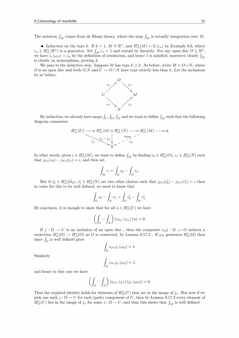
9 Cohomology of manifolds 58
The notation∫M
comes from de Rham theory, where the map∫M
is actually integration over M .
J Induction on the type k. If k = 1, M ∼= Rn, and Hnct(M) = Z 〈εn〉 by Example 9.6, where
εn ∈ Hnct (Rn) is a generator. Set
∫Mεn = 1 and extend by linearity. For any open disc O ⊆ Rn,
we have i∗ (ωO) = εn by the definition of orientation, and hence 1 is satisfied, moreover clearly∫M
is clearly an isomorphism, proving 2.We pass to the inductive step. Suppose M has type k ≥ 2. As before, write M = O∪N , where
O is an open disc and both O,N and U := O∩N have type strictly less than k. Let the inclusionsbe as before:
OjO
BBBBBBBB
U
iN @@@@@@@
iO
>>~~~~~~~M
N
jN
>>
By induction, we already have maps∫U,∫O,∫Nand we want to define
∫M
such that the followingdiagram commutes:
Hnct (U) //
∫U ((QQQQQQQQQQQQQQHn
ct (O)⊕Hnct (N)∫
O−∫N
// Hnct (M) //
want∫Mvvm m m m m m m
0
Z
In other words, given c ∈ Hnct(M), we want to define
∫M
by finding c0 ∈ Hnct(O), c1 ∈ Hn
ct(N) suchthat jO∗(c0)− jN∗(c1) = c, and then set∫
M
c :=∫O
c0 −∫N
c1.
But if c′0 ∈ Hnct(O0), c′1 ∈ Hn
ct(N) are two other choices such that jO∗(c′0) − jN∗(c′1) = c thenin order for this to be well defined, we need to know that∫
O
c0 −∫N
c1 =∫O
c′0 −∫N
c′1.
By exactness, it is enough to show that for all u ∈ Hnct(U) we have(∫
O
−∫N
)(iO∗, iN∗) (u) = 0.
If j : Ω → U is an inclusion of an open disc , then the composite iOj : Ω → O induces asurjection Hn
ct(Ω) → Hnct(O) as O is connected, by Lemma 9.17.3 . If ωΩ generates Hn
ct(Ω) thensince
∫O
is well defined gives ∫O
iO∗j∗ (ωΩ) = 1.
Similarly ∫N
iN∗j∗ (ωΩ) = 1,
and hence in this case we have(∫O
−∫N
)(iO∗, iN∗) (j∗ (ωΩ)) = 0.
Thus the required identity holds for elements of Hnct(U) that are in the image of j∗. But now if we
pick one such j : Ω→ U for each (path) component of U , then by Lemma 9.17.3 every element ofHn
ct(U) lies in the image of j∗ for some j : Ω→ U , and thus this shows that∫M
is well defined.

9 Cohomology of manifolds 59
Clearly∫M
then satisfies the required properties of (1), and moreover these determine∫M
uniquely, and thus this completes the proof of 1.2 is then immediate, by Lemma 9.17.3 we know that Hn
ct(M) is cyclic, and we claim that∫M
: Hnct(M)→ Z maps onto 1 ∈ Z, and thus is necessarily an isomorphism. To see this last claim
observe that if j : Ω → M is an open disc, then at least one of Ω ∩ O and Ω ∩ N is non-empty- without loss of generality assume that U ∩ N 6= ∅ and let k : Ω ∩ N → Ω and ` : Ω ∩ N → Ndenote inclusion maps. Then the following commutes
Ω ∩N k //
`
Ω
j
N
jN// M
The orientation condition implies that k∗ (ωΩ∩N ) = ωΩ, and then commutativity implies thatjN∗`∗ (ωΩ∩N ) = j∗ (ωΩ). Thus by definition∫
M
j∗ (ωΩ) =∫N
`∗ (ωΩ∩N ) = 1,
and this thus completes the proof of 2. I
We didn’t actually use the fact thatM was orientable until the end (although we used through-out the fact that O and N were). This motivates:
9.19 AddendumLet M,O,N be n-dimensional manifolds such that M = O ∪N with O and N orientable. Definethe map
∫M
: Hnct(M)→ Z as above. The following are equivalent:
1. Hnct(M) = Z,
2.∫M
is an isomorphism,
3. M is orientable.
J To see that 1⇒2, observe that if Hnct(M) = Z then jN∗ : Z→ Z is a surjective homomorphism
and hence an isomorphism. Thus if a generates Hnct(M) then there exists a generator b of Hn
ct(N)such that jN∗(b) = a, whence
∫Ma =
∫Nb = 1. Thus
∫M
is a homorphism that maps onto 1, andhence is an isomorphism.
2⇒ 1is trivial. 3⇒2 was proved in the previous proposition, and finally to see that 2⇒3 we use∫M
to define the specified generators ωO. Namely, let j : Ω → M denote an open disc. Thenj∗ : Hn
ct(Ω)→ Hnct(M) is an isomorphism (as again it is a surjective homomorphism Z→ Z, since
we already know2⇒ 1), and hence we can define a generator of Hnct(U) to be j−1
∗
((∫M
)−1 (1)).
This defines an orientation on M . I
We now complete the proof of Theorem 9.15 by proving:
9.20 PropositionLet Mn be a connected non-orientable manifold of finite type. Then Hn
ct(M) ∼= Z2.
J Since M has finite type there exists a cover M = O1 ∪ · · · ∪Ok with each Oi homeomorphicto an open disc, and all possible nested intersections either empty or homeomorphic to some opendiscs. Set Wi := O1 ∪ · · · ∪ Oi; we may assume that Wi is connected. The first claim we show isthat if Wi is orientable and Wi ∩Oi+1 is connected, then Wi+1 is orientable.
Indeed, we apply the Mayer-Vietoris sequence for compact supports (17) to Wi+1 = Wi ∪Oi+1
to obtain
Hnct (Wi ∩Oi+1)
φ→ Hnct (Wi)⊕Hn
ct (Oi+1)→ Hnct (Wi+1)→ Hn+1
ct (Wi ∩Oi+1) .
10 Poincaré duality 60
Suppose now that Wi ∪ Oi+1 = V1 t · · · t Vp, with each Vi connected. Since each Vi is anopen subset of Oi+1, they are all orientable. Moreover the inclusion map Vj → Oi+1 induces anisomorphism Hn
ct(Vj) → Hnct(Oi+1) (see the proof of Lemma 9.17). Hence φ is the map Zp → Z2,
and we may choose generators ωVi ∈ Hnct(Vi) such that φ (ωVi) = (∗, 1) in Hn
ct (Wi) ⊕Hnct (Oi+1),
where ∗ is some integer. But then since Wi is oriented, ∗ must be ±1 and thus φ is the map
jth place︷ ︸︸ ︷(0, . . . , 1, . . . 0)→ (±1, 1)
for each summand Vj .If all the images were the same, say (+1, 1) (which is necessarily the case if p = 1, that is,
Wi ∪Oi+1 is connected), then we would have coker φ ∼= Z, so Hnct(Wi+1) ∼= Z, and by Addendum
9.19 this would imply that we could orientate Wi+1.Since M is assumed to be non-orientable, we must have p > 1 for some i, and moreover for
some i such that p > 1 we must have not all the images being the same in Hnct (Wi)⊕Hn
ct (Oi+1)under φ. Thus in this case
coker φ =Z⊕ Z
〈(+1, 1), (−1, 1)〉= Z2,
and hence Hnct (Wi+1) ∼= Z2.
To complete the proof we show by induction that for i+ 1 ≤ j ≤ k we have Hnct (Wj) ∼= Z2 as
well. Indeed, if j < k then exactly the same argument now gives
Zp φ→ Z2 ⊕ Z→ Hnct (Wj)→ 0,
and the image under φ of each generator ωVi must be (1, 1). Thus Hnct (Wj) ∼= (Z2 ⊕ Z)/Z ∼= Z2,
and this completes the proof. I
We have finally completed the proof of Theorem 9.15, and thus have a complete description ofthe top dimensional cohomology of a compact connected manifold.
10 Poincaré duality
In this chapter we state and prove the key theorem of the course, Poincaré duality. We willgive two different versions of the theorem (Theorem 10.1 and Theorem 10.15). We will also brieflymention the intersection product, which can be thought of as the ‘Poincaré dual’ of the cupproduct.
10.1 Theorem (Poincaré duality)Let Mn be a closed connected orientable manifold. Then the pairing
Hk(M ; F)×Hn−k(M ; F)`→ Hn(M ; F)
∫M→ F,
(α, β) 7→∫M
α ` β
is non-degenerate (where F is any field). In particular, if α 6= 0 ∈ Hk(M ; F) then there existsβ ∈ Hn−k(M ; F) such that ∫
M
α ` β = 1.
If instead we take coefficients in Z and work modulo torsion then the pairing is still non-degenerate.Thus if α ∈ Hk(M ; Z) has infinite order and is a primitive element (that is, α cannot be written asrα′ for some α′ ∈ Hk(M ; Z) and r ∈ Z) then there exists β ∈ Hn−k(M ; Z) such that
∫Mα ` β = 1.
Before proving it we shall give some applications.
10 Poincaré duality 61
10.2 Computing the cohomology ring of CP n
We claim that H∗(CPn) = Z[α]/(αn+1), where α has degree 2 (that is, α ∈ H2(CPn) - written|α| = 2). Indeed, the inclusion CPn−1 → CPn induces an isomorphism on Hm for m ≤ 2n − 2(see Example 3.21). Thus by induction on n, H2m(CPn) is generated by αm for m < n by someα ∈ H2(CPn). By Poincaré duality there exists r ∈ Z such that∫
CPnα ` rαn−1 = 1.
Since∫
CPn is a homomorphism, this forces r = ±1. But then αn = α ` αn−1 generates Hn(CPn)(again as
∫CPn is a homomorphism), and this finishes the inductive step.
10.3 Showing S2 × S4 is not homotopy equivalent to CP3
Recall in Section 6.8 we showed that both S2 × S4 and CP 3 had the same additive homology,but we claimed that they were not homotopy equivalent. Using Poincaré duality, we are now in aposition to prove this. We will show that despite the fact they have the same additive cohomology(apply Theorem 5.29), they do not have the same ring structure.
First, we compute the cohomology ring of S2×S4. By Theorem 7.8, H∗(S2×S4) = H∗(S2)⊗H∗(S4). It is easy to see that H∗(Sn) = Z[β]/(β2) where |β| = n (trivially, by dimensionalreasons), and thus
H∗(S2 × S4) = Z[β]/(β2)⊗ Z[γ]/(γ2) = Z[β, γ]/(β2, γ2),
where β and γ have degree 2 and 4 respectively. This is clearly not isomorphic to the ringZ[α]/
(α4), which proves they are not homotopy equivalent.
Explicitly, by Poincaré Duality, and the fact that∫S2×S4 is an isomorphism, β ` γ generates
H6(S2 × S4). The cup product H2(S2 × S4) × H2(S2 × S4)`→ H4(S2 × S4) is identically zero,
since β ` β = 0. However the cup product H2(CP 3
)×H2
(CP 3
) `→ H4(CP 3
)is not identically
zero, since α2 ` α2 = α4 generates H4(CP 3
)and thus certainly isn’t zero.
10.4 DefinitionUsing Theorem 9.15 from the previous chapter we can extend Definition 4.1 to define the degreeof a map f : Mn → Nn between closed orientable connected manifolds. Indeed, by Theorem 9.15we have Hn(M) ∼= Hn (N) ∼= Z and thus f∗ : Hn(N) → Hn(M) is multiplication by an integerk := deg(f).
10.5 ExampleLet us show that if f : S4 → CP 2 then deg(f) = 0. Indeed, viewing H4(S4) as Z, the degree of fis f∗(α2), where α2 generates H4
(CP 2
). But as f∗ is a ring homomorphism by Lemma 7.4, we
have f∗(α2) = (f∗(α))2. However f∗(α) ∈ H2(S4) = 0. Thus deg(f) = 0, as claimed.Contrast this to the case f : S4 → S4, where by Corollary 4.11 f can have any integer degree.
Similarly there certainly exist maps CP 2 → CP 2 of non-zero degree (for instance, the identity).
Having given a few examples illlustrating the power of Theorem 10.1, we will now formulate anequivalent version of it, (which will be the version we will eventually prove). In order to do so wemust first introduce the cap product.
10.6 DefinitionLet R be a commutative ring with unit. The cap product is an R-bilinear map
a: Ck(X;R)× C`(X;R)→ Ck−`(X;R)

10 Poincaré duality 62
(for k ≥ `) defined byσ a ϕ := ϕ
(σ|[v0,...,v`]
)σ|[v`,...,vk]
for σ : ∆k → X and ϕ ∈ C`(X;R). From now on we shall assume that the coefficient ring is Z,and just write C∗(X) etc.
10.7 LemmaFor σ ∈ Ck(X) and ϕ ∈ C`(X),
d(σ a ϕ) = (−1)`(dσ a ϕ− σ a δϕ).
J Simply compute:
dσ a ϕ =∑i=0
(−1)iϕ(σ|[v0,...,vi,...,,v`+1])σ|[v`+1,...,vk] +
k∑i=`+1
(−1)iϕ(σ|[v0,...,v`])σ|[v`,...,vi,...,vk],
σ a δϕ =`+1∑i=0
(−1)iϕ(σ|[v0,...,vi,...,v`+1])σ|[v`+1,...,vk].
Next,
d(σ a ϕ) =k∑i=`
(−1)i−`ϕ(σ|[v0,...,v`])σ|[v`,...,vi,...,vk].
The stated formula visibly holds. I
10.8 CorollaryThe cap product a descends to give a well defined map
a: Hk(X)×H`(X)→ Hk−`(X).
J From the relation d(σ a ϕ) = ±(dσ a ϕ − σ a δϕ) it follows that the cap product of acycle σ and a cocycle ϕ is a cycle. Further, if dη = σ and δϕ = 0 then d(η a ϕ) = ±(σ a ϕ), andthus the cap product of a boundary and a cocycle is a boundary, and if δψ = ϕ and dσ = 0 thend(σ a ψ) = ±(σ a ϕ) and thus the cap product of a cycle and a coboundary is also a boundary.These are precisely the conditions needed to ensure that a descends to give a well defined map onhomology and cohomology. I
10.9 LemmaLet f : X → Y . Then for α ∈ Hk(X) and β ∈ H`(Y ) we have
f∗(α) a β = f∗(α a f∗(β)).
J Let σ represent α and ϕ represent β. Then
fσ a ϕ = ϕ(fσ|[v0,...,v`])fσ|[v0,...,vk]
= f(ϕ(fσ|[v0,...,v`])σ|[v`,...,vk]
= f(σ a ϕf). I
10.10 LemmaFor σ ∈ Ck+`(X), ϕ ∈ Ck(X) and ψ ∈ C`(X) we have
ψ(σ a ϕ) = (ϕ ` ψ)(σ).
J Let σ : ∆k+` → X be a singular (k + `)-simplex. Then
ψ(σ a ϕ) = ψ(ϕ(σ|[v0,...,vk]
)σ|[vk,...,vk+`]
)= ϕ
(σ|[v0,...,vk]
)ψ(σ|[vk,...,vk+`]
)= (ϕ ` ψ)(σ). I

10 Poincaré duality 63
10.11 DefinitionLet M be a closed orientable manifold with specified orientation µxx∈M . By Theorem 9.11,there exists an element [M ] := µM ∈ Hn (M) (taking K = M in Theorem 9.11) with the propertythat for any x ∈M we have [M ] |x = µx (that is, the image of [M ] in Hn (M |x) under the naturalmap Hn (M)→ Hn (M |x) is µx. We call [M ] the fundamental class of M .
10.12 LemmaLet M be a closed orientable connected n-manifold. Then if α ∈ Hk(M), β ∈ Hn−k(M)∫
M
α ` β = (α ` β)[M ].
J It is enough to check this for α ` β = ω a generator of Hnct (M). Clearly if ω is a generator
then∫Mω = ω ([M ]) = 1. I
10.13 The duality mapFor a closed orientable manifold M , this gives us a duality map
D : Hk(M)→ Hn−k(M)
given by D(α) = [M ] a α. This gives us another way to state Poincaré duality. Before doing so,however we want to define a duality map for non-compact manifolds.
10.14 The duality map on non-compact manifoldsSuppose K ⊆ L are compact sets, and i : M\L → M\K the inclusion map. By uniquenessof µK , the image i∗(µL) ∈ Hn(M |K) must be µK . Moreover, by Lemma 10.9 we have for anyα ∈ Hk(M |K)
µK a α = i∗(µL) a α = µL a i∗(α),
and thus if we define DK : Hk(M |K) → Hn−k(M) by DK(α) = µK a α then the DK arecompatible with taking the direct limit, and hence the DK induce in the direct limit a dualityhomomorphisms
D : Hkct(M) := lim−→
K⊆M compact
Hk(M |K)→ Hn−k(M).
Note that if M is closed, then D is just the duality map from Definition 10.13, since all thecompact subsets of M are then contained in the compact set M .
Now we can state the alternative version of Poincaré duality. Note this version holds for allorientable connected manifolds - we no longer require that M be closed.
10.15 Theorem (Poincaré duality - alternative version)Let Mn be an orientable connected manifold of finite type. Then the duality map D : Hk
ct(M)→Hn−k(M) is an isomorphism for all 0 ≤ k ≤ n.
The assumption of finite type is unnecessary; an application of Zorn’s lemma will remove thiscondition. The result actually holds with coefficients in any commutative ring with unit; the proofis exactly the same. Like Theorem 9.15, we will prove this by induction on type.
First of all, we check the two statements of Poincaré duality coincide for closed manifolds.

10 Poincaré duality 64
10.16 LemmaTheorem 10.15 is equivalent to Theorem 10.1 for closed orientable connected manifolds.
J Observe that if we work over a field F then Hn−k(M ; F) ∼= Hn−k(M ; F) (see Addendum2.9). Consider the composition
Hn−k(M ; F) h→ Hom(Hn−k(M ; F),F) D∗
→ Hom(Hk(M ; F),F),
where h is the map of Lemma 2.8. Now D∗h sends β ∈ Hn−k(M ; F) to the homomorphism definedby (where ψ is a cocycle representing β)
α 7→ [ψ([M ] a α)] = (α ` β)[M ] =∫M
α ` β,
by Lemma 10.10 and Lemma 10.12. Thus non-singularity of one of the variables in the pairing(α, β) 7→
∫Mα ` β is equivalent to D being an isomorphism (non-singularity of the other variable
then follows from skew-commutativity of `). IWe will now finally give a proof of Poincaré duality. We will prove the more general version,
Theorem 10.15. The difficult part of the proof is the assertion that a certain diagram commutes.
10.17 Key LemmaLet Mn be an orientable manifold, and suppose M = U ∪ V , with U, V open. Then there is adiagram of Mayer-Vietoris sequences, commutative up to a sign:
. . . // Hkct (U ∩ V ) //
DU∩V
Hkct (U)⊕Hk
ct (V ) //
DU⊕−DV
Hkct (M) //
DM
Hk+1ct (U ∩ V ) //
DU∩V
. . .
. . . // Hn−k (U ∩ V ) // Hn−k (U)⊕Hn−k (V ) // Hn−k (M) // Hn−k−1 (U ∩ V ) // . . .
J Let K ⊆ U and L ⊆ V be compact. They give rise to the Mayer-Vietoris sequence in theupper row of the following diagram, whose lower row is also a Mayer-Vietoris sequence.
Hk (M |K ∩ L)
∼=
// Hk (M |L)⊕Hk (V |L)
∼=
// Hk (M |K ∪ L) ∂∗ // Hk+1 (M |K ∩ L)
∼=
Hk (U ∩ V |K ∩ L)
µK∩La
Hk (U |K)⊕Hk (V |L)
µKa⊕−µLa
Hk (U ∪ V |K ∪ L)
µK∪La
Hk+1 (U ∩ V |K ∩ L)
µK∩La
(F)
Hn−k (U ∩ V ) // Hn−k (U)⊕Hn−k (V ) // Hn−k (M) ∂ // Hn−k−1 (U ∩ V )
The three maps labelled isomorphisms come from excision. Assume for now that this diagramcommutes up to a sign. Consider passing to the limit over compact sets K ⊆ U and L ⊆ V . Sinceeach compact set in U ∩ V is contained in an intersection K ∩ L of compact subsets K ⊆ U andL ⊆ V , and similarly for U ∪ V , the diagram induces a limit diagram having the form stated inthe lemma. The first row of this limit diagram is exact since the direct limit of exact sequences inexact (by the exactness principle from the proof of Lemma 9.14). Thus showing commutativity(up to a sign) of (F) is enough to prove the lemma.
The first two squares of (F) are easily seen to commute at the chain level. Much less simple isthe third square, which we will show commutes up to a sign. Set A = M\K and B = M\L. Themap ∂∗ is obtained from the following short exact sequence of cochain complexes:
0→ C∗(M,A+B)→ C∗(M,A)⊕ C∗(M,B)→ C∗(M,A ∩B)→ 0.
To evaluate the Mayer-Vietoris coboundary map ∂∗ on a cohomology class represented by a cocycleϕ ∈ C∗(M,A ∩B), first write ϕ = ϕA − ϕB for ϕA ∈ C∗(M,A) and ϕB ∈ C∗(M,B). Then ∂∗[ϕ]

10 Poincaré duality 65
is represented by the cocycle δϕA = δϕB ∈ C∗(M,A + B). Similarly, if z ∈ C∗(M) represents ahomology class in H∗(M) then ∂[z] = [dzU ], where z = zU −zV with zU ∈ C∗(U) and zV ∈ C∗(V ).
Via barycentric subdivision, the class µK∪L can be represented by a chain α that is a sumα = αU\L + αU∩V + αV \K of chains in U\L, U ∩ V and V \K respectively, since these three openset cover M . By unqiueness of µK∩L the chain αU∩V represents µK∩L, since the other two chainslie in the complement of K ∩ L and thus vanish in Hn(M |K ∩ L) ∼= Hn(U ∩ V |K ∩ L). Similarlythe chain αU\L + αU∩V represents µK .
Now let ϕ be a cocycle representing an element of the top left-hand group of the previousdiagram, Hk(M |K ∪ L), Under ∂∗, this maps to the cohomology class of δϕA. Continuing downto the bottom right-hand corner, Hn−k−1(U ∩ V ), we obtain αU∩V a δϕA, which is the samehomology class as dαU∩V a ϕA by Lemma 10.7, as
d(αU∩V a ϕA) = (−1)k (dαU∩V a ϕA − αU∩V a δϕA) ,
and αU∩V a ϕA is a chain in U ∩ V , so the two terms differ by a boundary and thus are the sameas far as homology is concerned.
Now going round the other way, ϕ is first mapped to α a ϕ ∈ Hn−k(M). Write this as a sumof a chain in U and a chain in V :
α a ϕ =(αU\L a ϕ
)+(αU∩V a ϕ+ αV \K a ϕ
),
and hence by definition,
∂[α a ϕ] =[d(αU\L a ϕ
)]∈ Hn−k−1(U ∩ V ).
Then we compute
d(αU\L a ϕ
)= (−1)kdαU\L a ϕ(∗)= (−1)kdαU\L a ϕA
(∗∗)= (−1)k+1dαU∩V a ϕA,
where (∗) follows as dαU\L a ϕB = 0, since as ϕB is zero on chains in B = M\L, and (∗∗) followssince d(αU\L+αU∩V ) a ϕA = 0, as d(αU\L+αU∩V ) is a chain in U\K (by the earlier observationthat αU\L + αU∩V represents µK , and ϕA vanishes on chains in A = M\K).
Thus we have shown that the last diagram commutes up to a sign, and this completes the proofof the lemma. I
Finally we can prove Poincaré duality.J Proof of Theorem 10.15: Induction on type. First we prove the result for Rn. Regard
Rn as the interior of ∆n, and then the map D can be identified with the map Hk(∆n, ∂∆n) →Hn−k(∆n) given by cap prodict with a unit times the generator [∆n] ∈ Hn(∆n, ∂∆n) defined bythe identity map, which is a relative cycle. The only non-trivial value is k = n, when the capproduct map is an isomorphism since a generator of Hn(∆n, ∂∆n) ∼= Hom(Hn(∆n, ∂∆n),Z) isrepresented by a cocycle taking the value 1 on ∆n, so by definition of the cap product, [∆n] a ϕis the last vertex of ∆n, representing a generator of H0(∆n).
Passing to the inductive step, suppose M has type k ≥ 2. Write M = U ∪ V , where U ishomeomorphic to Rn and both U and U ∩ V have type strictly less than k. We then apply thefive lemma (Lemma 3.10) to the the diagram that the Key Lemma asserts commutes up to a sign(the five lemma still holds, despite the fact that the diagram only commutes up to a sign - theproof of the five lemma goes through word for word) to see that DM : Hk
ct(M)→ Hn−k(M) is anisomorphism, and this completes the proof. I
We now define the Poincaré dual cohomology class of a given submanifold.
10.18 DefinitionLetMn be a closed oriented manifold and Y n−k a closed oriented submanifold. The inclusion mapi : Y → M induces i∗ : Hn−k(Y ) → Hn−k(M), and then the inverse of the Poincaré duality map

11 The Thom isomorphism theorem 66
gives us a map D−1 : Hn−k(M)→ Hkct(M) = Hk(M). Let εY denote the image
εY := D−1(ι∗[Y ]) ∈ Hk(M).
εY is called the Poincaré dual cohomology class Y ; note that εY lives in the cohomology groupM of dimension the codimension of Y in M . By definition, we have
[M ] a εY = i∗[Y ].
Since D−1 is an isomorphism, εY is unique.Note that if α ∈ Hn−k(M) then∫
M
α ` εY = α ` εY [M ]
= α ([M ] a εY )= α(i∗[Y ])= i∗α([Y ])
=∫Y
α|Y ,
and moreover εY is the unique class in Hk(M) with this property.
We wish however to give a direct definition of the Poincaré dual class without using Poincaréduality, at least in the case that M and Y are smooth. To do this, we first need to state and provethe Thom isomorphism theorem, which is the subject of the next chapter.
11 The Thom isomorphism theorem
We begin this chapter with a quick recap of the definition of a vector bundle.
11.1 DefinitionsLet M be a manifold. A vector bundle π : E → M of rank n is a family of n-dimensional realvector spaces, Exx∈M , with E :=
⊔x∈M Ex and π : E → M mapping Ex onto x, equipped
with a topology for which π is continuous and the following local triviality condition holds:
• For each x ∈M there exists a neighborhood U of x and a homeomorphsim
t : E|U := π−1(U)→ U × Rn
which is fibre preserving in the sense that for all y ∈ U the restriction ty := pr2t : Ey → Rnis a vector space isomorphism.
The space E is called the total space, and M is called the base space. The map π is called theprojection.
A continuous map s : M → E such that πs = 1 is called a section of E. One obvious sectionis the map o : M → E mapping x 7→ 0 ∈ Ex, which is called the zero section. By an abuse ofterminology, the image o(M) ⊆ E is also called the zero section. We let E# denote the complementof the zero section in E.
Note that o(M) is homeomorphic to M , and that E is homotopic to o(M) via the linearhomotopy in each vector space Ex. Moreover the map π : E → M induces an isomorphismπ∗ : H∗(M) → H∗(E), since the zero section embeds M as a deformation retraction of E, withthe retraction mapping being π. Similarly o∗ : H∗ (E)→ H∗ (M) is an isomorphism.
Next, we survey three standard vector bundle constructions; the pullback bundle, the Whit-ney sum and the normal bundle.
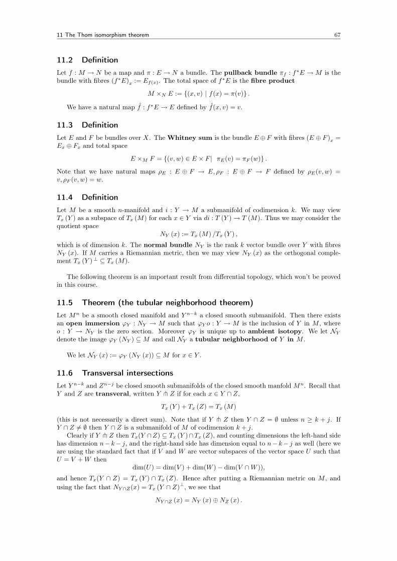
11 The Thom isomorphism theorem 67
11.2 DefinitionLet f : M → N be a map and π : E → N a bundle. The pullback bundle πf : f∗E →M is thebundle with fibres (f∗E)x := Ef(x). The total space of f∗E is the fibre product
M ×N E := (x, v) | f(x) = π(v) .
We have a natural map f : f∗E → E defined by f(x, v) = v.
11.3 DefinitionLet E and F be bundles over X. The Whitney sum is the bundle E⊕F with fibres (E ⊕ F )x =Ex ⊕ Fx and total space
E ×M F = (v, w) ∈ E × F | πE(v) = πF (w) .
Note that we have natural maps ρE : E ⊕ F → E, ρF : E ⊕ F → F defined by ρE(v, w) =v, ρF (v, w) = w.
11.4 DefinitionLet M be a smooth n-manifold and i : Y → M a submanifold of codimension k. We may viewTx (Y ) as a subspace of Tx (M) for each x ∈ Y via di : T (Y )→ T (M). Thus we may consider thequotient space
NY (x) := Tx (M) /Tx (Y ) ,
which is of dimension k. The normal bundle NY is the rank k vector bundle over Y with fibresNY (x). If M carries a Riemannian metric, then we may view NY (x) as the orthogonal comple-ment Tx (Y )⊥ ⊆ Tx (M).
The following theorem is an important result from differential topology, which won’t be provedin this course.
11.5 Theorem (the tubular neighborhood theorem)Let Mn be a smooth closed manifold and Y n−k a closed smooth submanifold. Then there existsan open immersion ϕY : NY → M such that ϕY o : Y → M is the inclusion of Y in M , whereo : Y → NY is the zero section. Moreover ϕY is unique up to ambient isotopy. We let NYdenote the image ϕY (NY ) ⊆M and call NY a tubular neighborhood of Y in M .
We let NY (x) := ϕY (NY (x)) ⊆M for x ∈ Y .
11.6 Transversal intersectionsLet Y n−k and Zn−j be closed smooth submanifolds of the closed smooth manfoldMn. Recall thatY and Z are transveral, written Y t Z if for each x ∈ Y ∩ Z,
Tx (Y ) + Tx (Z) = Tx (M)
(this is not necessarily a direct sum). Note that if Y t Z then Y ∩ Z = ∅ unless n ≥ k + j. IfY ∩ Z 6= ∅ then Y ∩ Z is a submanifold of M of codimension k + j.
Clearly if Y t Z then Tx(Y ∩Z) ⊆ Tx (Y )∩Tx (Z), and counting dimensions the left-hand sidehas dimension n− k− j, and the right-hand side has dimension equal to n− k− j as well (here weare using the standard fact that if V and W are vector subspaces of the vector space U such thatU = V +W then
dim(U) = dim(V ) + dim(W )− dim(V ∩W )),
and hence Tx(Y ∩ Z) = Tx (Y ) ∩ Tx (Z). Hence after putting a Riemannian metric on M , andusing the fact that NY ∩Z(x) = Tx (Y ∩ Z)⊥, we see that
NY ∩Z (x) = NY (x)⊕NZ (x) .
11 The Thom isomorphism theorem 68
11.7 AddendumLet Y n−k and Zn−j be closed smooth submanifolds of the closed smooth manfoldMn, and supposethat Y t Z. Then we may choose the tubular neighborhoods ϕY : NY → NY , ϕZ : NZ → NZ andϕY ∩Z : NY ∩Z → NY ∩Z such that
NY ∩Z (x) = NY (x)×NZ (x)
for all x ∈ Y ∩ Z.
11.8 DefinitionWe say that a rank n vector bundle π : E → M is oriented if for each x ∈ M there exists aneighborhood U of x, a local trivialisation t : E|U → U × Rn, generators φy ∈ Hn
ct (Ey) for y ∈ Uand a generator εn ∈ Hn
ct (Rn) such that ty∗ (φy) = εn for all y ∈ U . We say the collection φxx∈Mis an orientation of E.
It can be shown that if M is smooth then M is orientable if and only T (M) is orientable as avector bundle, and an orientation of one determines an orientation of the other.
Now let π : E →M be an oriented vector bundle of rank n. We will show that the interestingcohomology of E is actually H∗(E,E#) which is in some sense the cohomology ‘close’ to M . Inwhat follows, let
j : (E, ∅) →(E,E#
), jx :
(Ex, E
#x
)→(E,E#
)for x ∈ M denote inclusions (where E#
x := Ex\0). Given α ∈ H∗(E,E#
), write α|Ex for
j∗x(α) ∈ H∗(Ex, E
#x
), and similarly α|E for j∗(α) ∈ Hn(E). The following crucial theorem is the
main result of this chapter.
11.9 Theorem (the Thom isomorphism theorem)Let π : E → M be an oriented vector bundle of rank n with orientation φxx∈M . The followingholds:
1. Hm(E,E#
)= 0 for m < n.
2. There exists a unique element uE ∈ Hn(E,E#
), called the Thom class such that for all
x ∈M , the restriction uE |Ex = φx,
3. The map T : Hm(M)→ Hm+n(E,E#
)defined by
T (α) := π∗α ` uE
is an isomorphism. T is called the Thom isomorphism. Note that T (1) = uE , for 1 ∈H0(M).
J We will prove this under the assumption that M has a finite trivialising cover for E, which isalways true if M is compact or has finite type, since it can be shown that every vector bundle overa contractible space (like a disc) is trivial. However this assumption is made just to simplify theproof; in fact the theorem is true for arbitary manifolds.
Step 1: First consider the base case of the trivial bundle E ∼= M × Rn.Let Z ⊆ Y where Y has finitely generated and free cohomology. By the Kunneth theorem
(Theorem 7.8) we haveH∗(M)⊗H∗(Y,Z) ∼= H∗(M × Y,M × Z)
(this is actually a relative version of Theorem 7.8). In particular, taking (Y, Z) = (Rn,Rn\0) weobtain
H∗(M)⊗H∗(Rn|0) ∼= H∗(E,E#),
and henceHm(E,E#) ∼= Hm−n(M)⊗ Z ∼= Hm−n(M).
11 The Thom isomorphism theorem 69
This proves 1 and 3 in this special case. Now define uE to be εn where εn generates Hnct(Rn). 2 is
then clearly satisfied.
Step 2: We pass to the inductive step. Suppose M has a trivialising cover of E consisting ofr elements. Write X = V ∪W where each V,W are open in X and E|V ,E|W and E|V ∩W all havetrivialising covers consisting of strictly less than r elements. Considering the long exact sequenceof the pair (E,E#) we can write
Hm−1(E|V ∩W , E#|V ∩W
)→ Hm
(E,E#
)→ Hm
(E|V , E#|V
)⊕Hm
(E|W , E#|W
)→ Hm
(E|V ∩W , E#|V ∩W
),
and thus by induction we see that 1 immediately holds, as for m < n the sequence reduces to
0→ Hm(E,E#)→ 0.
For m = n, we obtain
0→ Hn(E,E#
)→ Hn
(E|V , E#|V
)⊕Hn
(E|W , E#|W
)→ Hn
(E|V ∩W , E#|V ∩W
)→ . . .
By induction, the Thom classes uE|V , uE|W exist and are unique. By uniqueness, they must havethe same image in E|V ∩W , namely uE|V∩W and thus they come from a common cohomology classuE ∈ Hn(E,E#). This class is uniquely defined, since Hn−1(E,E#) = 0.
Step 3: Consider the following diagram:
Hm+n(E|V , E#|V
)⊕Hm+n
(E|W , E#|W
)// Hm+n
(E|V ∩W , E#|V ∩W
)∂∗E // Hm+n+1(E,E#
)
Hm (V )⊕Hm (W ) //
∼=T
OO
Hm (V ∩W ) ∂∗ // Hm+1(M)
T
OO
If we could show it commuted then the five lemma (applied to the five terms) would give thatthe right-hand T was also an isomorphism. Since commutativity of the first square is obvious, soit remains to show that the second square commutes.
We already know uE exists, and thus we may choose a cocycle ϕ ∈ Ck+n(E,E#) representinguE . Then ϕ restricts to a cocycle on E|V , E|W and E|V ∩W thus by uniqueness the restrictionsϕ|E|V , ϕ|E|W and ϕ|E|V∩W represent the Thom classes E|V , E|W and E|V ∩W respectively. Nowtake α ∈ Hk(V ∩W ) and ψ a cocycle representing α. Suppose ∂∗(α) = β ∈ Ck+1(X). Then if wewrite ψ = ψV − ψW where ψV ∈ Ck(V ), ψW ∈ Ck(W ), we have δ(ψV ) representing β.
Now by definitionT∂∗(α) = π∗(β) ` uE = π∗[δψV ] ` uE .
Next,
∂∗ET (α) = ∂∗E(π∗(α) ` uE|V∩W
)= δE
(π∗[ψV ] ` [ϕE|V ]
),
since we can write
π∗(α) ` uE|V∩W = π∗[ψV ] ` [ϕE|V ]− π∗[ψW ] ` [ϕE|W ],
withπ∗[ψV ] ` [ϕE|V ] ∈ Ck(E|V , E#|V ),
π∗[ψW ] ` [ϕE|W ] ∈ Ck(E|W , E#|W ).
Finally, the differential δE clearly commutes with π∗ as π∗ is a cochain map and hence
δE(π∗[ψV ] ` [ϕE|V ]) = π∗[δψV ] ` uE ,
and the second square commutes as required. This completes the proof. I
We now introduce another extremely important cohomology class associated to a vector bundle.The reason for the name will be explained in Theorem 12.10.

11 The Thom isomorphism theorem 70
11.10 DefinitionWe can obtain an element of Hn(M) corresponding to the Thom class uE under the composition
Hn(E,E#)j∗→ Hn(E) o∗→ Hn(M),
where o : M → E is the zero section. We write e(E) for the image of uE in Hn(M) and call e(E)the Euler class of the bundle π : E →M .
11.11 DefinitionA rule E 7→ c(E) which associates to every vector bundle E →M of a certain type a cohomologyclass c(E) ∈ H∗(M) is called a characteristic class if it is natural with respect to pullbacks inthe sense that c (f∗E) = f∗(c(E)).
11.12 LemmaThe Euler class is a characteristic class for real oriented vector bundles.
J In order to prove this we first need to define the induced orientation on a pullback bundle.Let f : M → N be map between manifolds and π : E → N a real oriented vector bundle of rank nwith orientation φxx∈N . Then the induced orientation on f∗E is ψpp∈M where by definition
ψp := f∗(φf(p)
)∈ Hn
ct(Ef(p)
),
where f∗ : Hnct(Ef(p)
)→ Hn
ct
((f∗E)p
).
The map
Hn(f∗E, (f∗E)#
)→ Hn (f∗E)
π∗f→ Hn(M)
surjects, so let α be a preimage of f∗(e(E)) in Hn(f∗E, ((f∗E)#
). The following commutes:
Hn(E,E#
)// Hn (E)
f∗
o∗E // Hn (N)
f∗
Hn
(f∗E, (f∗E)#
)// Hn (f∗E)
o∗f∗E
// Hn (M)
Now let p ∈M . Then commutativity forces
α|(f∗E)p= f∗x
(uE |Ef(p)
)= f∗x
(φf(p)
)= ψp,
and thus by uniqueness of the Thom class, α = uf∗E , and hence
e (f∗E) = f∗ (e(E)) ,
which is what we wanted to show. I
Here are three results on the vanishing of the Euler class.
11.13 CorollaryA trivial vector bundle has zero Euler class.
J Let f : M → pt. Consider the vector bundle τ : Rn → pt. Then certainly e (Rn) = 0.Moreover f∗Rn is the trivial vector bundle M × Rn, and hence by the previous lemma,
e (M × Rn) = f∗ (e (Rn)) = f∗ (0) = 0. I

11 The Thom isomorphism theorem 71
11.14 LemmaIf E → M has a nowhere-zero section (that is, a section s : M → E such that s(M) ∩ o(M) = ∅)then e(E) = 0.
J Since s is never zero the following composition is the identity:
Hn(M) π∗
→ Hn (E) k∗→ Hn(E#) s∗→ Hn(M),
where k : E# → E is inclusion. By definition the first map carries e(E) to uE |E , and thus thefirst two maps take e(E) to (u|E)|E# , which is zero since the composition
Hn(E,E#)j∗→ Hn(E) k∗→ Hn(E#)
is zero by exactness. Applying s∗, we see that e(E) = s∗(0) = 0. I
11.15 LemmaIf π : E → M has odd rank 2n + 1 then e(M) ∈ H2n+1(M) has order two. In particular ifH2n+1(M) is torsion-free then e(E) = 0.
J Under the Thom isomorphism T, by definition we have
T (e(E)) = π∗(e(E)) ` uE= uE ` uE= −(uE ` uE),
since α ` β = −(β ` α) for α, β ∈ H2n+1(X) by Proposition 7.5. Thus T (e(E)) is 2-torsion, andsince T is an isomorphism the same is true of e(E) too. I
11.16 Poincaré duals revisitedLetMn be a closed smooth manifold and Y n−k a closed smooth submanifold which is cooriented,that is, the normal bundle NY is an orientated vector bundle. Let ϕY : NY → NY be a tubularneighborhood of Y . Then the Thom class uNY ∈ Hk
(NY , N
#Y
)determines a class εY ∈ Hk(M)
under the map
Hk(NY , N
#Y
) (ϕ−1Y )∗−→ Hk (NY ,NY \Y ) ∼→ Hk(M,M\Y )→ Hk (M) .
The reader may note that this is the same notation we used for the Poinaré dual class of Y inHk (M) defined at the end of the last chapter (Definition 10.18). This is no coincidence; in fact,these are one and the same cohomology class. Thus this is the promised definition of the Poincarédual class which does not use Poincaré duality (note that the proof of Theorem 11.9 did not usePoincaré duality).
Between now and the completion of the proof of Corollary 11.22 (which states that the twodefinitions are equivalent) the notation εY refers to this definition, not the one from Definition10.18.
11.17 LemmaLet Mn be a smooth closed orientable manifold, Y n−k a closed submanifold and εY ∈ Hk(M) theclass defined above. Then
εY |Y = e (NY ) ,
that is, under the map i∗ : Hk(M) → Hk(Y ) induced from the inclusion i : Y → M we havei∗(εY ) = e (NY ).

11 The Thom isomorphism theorem 72
J Let ϕY : NY → NY be a tubular neighborhood of Y , and let o : Y → NY be the zerosection. The following commutes:
Hk (M,M\Y )
excision
// Hk (M)i∗
%%KKKKKKKKK
Hk (NY ,NY \Y ) // Hk (NY ) // Hk (Y )
Hk(NY , N
#Y
)(ϕ−1Y )∗
OO
// Hk (NY )
o∗
::uuuuuuuuuu
Commutativity of the diagram gives the result. I
11.18 PropositionLet π : E → M be a rank k bundle and τ : F → M a rank ` bundle. Then the Thom class ofE ⊕ F is
ρ∗EuE ` ρ∗FuF ,
where ρE and ρF are the projections (see Definition 11.3).
J Note that the following diagram commutes:
Hkct(Rk) × H`
ct(R`)×→ Hk+`
ct (Rk+`)↓ ↓ ↓ (♠)
Hk(Sk) × H`(S`) ×→ Hk+`(Sk × S`)
The bottom row by is an isomorphism by the Kunneth theorem (Theorem 7.8) and the verticalmaps are isomorphisms by the computations in Example 9.6. Hence the top line of the diagram isalso an isomorphism.
To prove the result, simply observe ρ∗EuE ` ρ∗FuF is a class in Hk+`(
(E ⊕ F ) , (E ⊕ F )#),
and commutativity of the diagram above ensures that the restriction to each fibre of ρ∗EuE ` ρ∗FuF
is the preferred generator of Hk+`ct (Ex ⊕ Fy). Uniqueness of the Thom class then shows uE⊕F =
ρ∗EuE ` ρ∗FuF as claimed. I
The next remark is trivial but highly useful.
11.19 LemmaLet Mn be a smooth closed orientable manifold, Y n−k a closed coorientable submanifold andεY ∈ Hk(M) the class defined in Section 11.16. Let ϕY : NY → NY denote a tubular neighborhoodof Y , and let φxx∈Y denote the orientation on NY . Then εY is represented by any cocycleψ ∈ Ckct(M) such that
• ψ is supported in NY (that is, ψ|M\NY = 0),
• for all y ∈ NY ψ|NY (x) represents the distinguished generator of φx ∈ Hkct (NY (x)) given by
the orientation on N under the isomorphism ϕ∗Y : Hkct (NY (x))→ Hk
ct (NY (x)).
This is immediate from the uniqueness up to ambient isotopy of ϕY : NY → NY in the tubularneighborhood theorem and the uniqueness of the Thom class.

11 The Thom isomorphism theorem 73
11.20 PropositionLet Y n−k and Zn−j be transverse co-oriented closed submanifolds of the smooth closed manifoldMn. Then εY ∩Z = εY ` εZ . Hence the cup product is ’Poincaré dual’ to intersection.
J From Addendum 11.7 we may take NY ∩Z (x) = NY (x) × NZ (x) for all x ∈ Y ∩ Z.Let ψY ∈ Hk (M) represent εY , ψZ ∈ Hj (M) represent εZ and qY : NY ∩Z (x) → NY (x),qZ : NY ∩Z (x)→ NZ (x) br projections. Let
φYxx∈Y and
φZxx∈Z be the orientations of NY and
NZ . Then (ψY ` ψZ) |NY∩Z(x) represents q∗Y φYx ` q∗Zφ
Zx in Hk+j
ct (NY ∩Z (x)) by the commutativediagram (♠) given in the proof of Proposition 11.18. Since ψY ` ψZ clearly vanishes onM\NY ∩Z ,by Lemma 11.19 it follows that ψY ` ψZ represents εY ∩Z , and this completes the proof. I
11.21 PropositionLetMn be a smooth closed orientable manifold, and Y n−k a smooth closed coorientable connectedsubmanifold of M . Then ∫
M
α ` εY =∫Y
α|Y for all α ∈ H∗(Y ). (19)
J We successively reduce to increasingly special cases. Let ϕY : NY → NY denote a tubularneighborhood of Y in M . It is sufficient to show that∫
NY
ϕ∗Y α ` uNY |NY =∫Y
α|Y .
In fact, if i : Y →M denotes inclusion and o : Y → NY the zero section then since ϕY o = i, ifπ : NY → Y is the projection map then ϕY is homotopic to iπ, and thus we need only show thatfor all β ∈ Hn−k (Y ), ∫
NY
π∗β ` uNY |NY =∫Y
β. (20)
Now if j : O → Y be an open disc in Y , so j∗ : Hn−kct (O) → Hn−k
ct (Y ) is surjective by Lemma9.17.3, and hence it suffices to prove (20) for β ∈ im j∗. In fact, it is enough to show that if ωO isour prescribed generator of Hn
ct(O) then∫N
ϕ∗Y j∗ (ωO) ` uNY |NY = 1,
since by definition of∫Y
we have ∫Y
j∗ (ωO) = 1
(see Proposition 9.18.1.Now since O is a disc, E|O ∼= O × Rk since any bundle over a disc is trivial12. Let t : NY |O →
O × Rk denote the trivialisation. Then making use of the commutative diagram (♠) from theproof of Proposition 11.18 shows that pr∗1 (ωO) ` pr∗2(εk) generates Hn
ct(O × Rk
), where εk is a
generator of Hkct(Rk), and moreover
t−1∗ (pr∗1 (ωO) ` pr∗2 (εk)) = (π∗ (j∗ (ωO)) ` uNY ) |NY |O ,
since by uniqueness of the Thom class, uNY |NY |O is precisely pr∗2(εk). But then since by definitionof∫NY
we have ∫NY
t−1∗ (pr∗1 (ωO) ` pr∗2 (εk)) = 1,
it follows that ∫NY
π∗ (j∗ (ωO)) ` uNY |NY = 1
as required. I12 If we don’t want to quote this result, just taking O small enough so that it is contained in a single trivialising
neighborhood also works

11 The Thom isomorphism theorem 74
11.22 CorollaryThe two definitions of εY (Definition 10.18 and Section 11.16) conicide.
J Immediate, since we know that the class εY from Definition 10.18 is the unique class sat-isfying (19). I
Using Poincaré dual classes of submanifolds we can often obtain valuable information geomet-rically. Here are three examples.
11.23 Example: the Hopf bundleThe Hopf bundle π : S3 → S2 is the fibre bundle defined by
π : (z1, z2) ∈ S3 ⊆ C2 7→ (z1 : z2) ∈ CP 1 = S2,
with each fibre isomorphic to S1 (a great circle on S3). We claim there is no global section s of π.Indeed, suppose s : S2 → S3 is a global section. Then S3 has submanifolds Y := s
(S2) ∼= S2
and Z := h−1(p) ∼= S1, where p is any point in S2. Clearly Y ∩ Z = s(p), moreover one canshow that the intersection is tranverse. Since H1
(S3)
= H2
(S3)
= 0, the fundamental classes[S1]∈ H1
(S3)and
[S2]∈ H2
(S2)are both zero. Thus the same is true of εY and εZ . Then by
Proposition 11.20, it follows εY ∩Z = 0, and hence [s (p)] = 0 ∈ H0
(S3). But this is clearly false,
as [pt] ∈ H0
(S3)is never zero13.
11.24 Determining the homology of Σ2
Consider Σ2, the torus with two holes. We can consider 4 obvious curves on Σ2 that represent gen-erators of H1(Σ2). One way to see that they are actually generators is to use simplicial homology,and construct an explicit triangulation. Here is another.
Label the circles c, γ, c′, γ, where c and γ are two loops round the first hole, and c′ and γ′ areloops round the second hole. Then c and γ intersect transversely, and thus [c ∩ γ] = [pt] 6= 0,and so dualizing we see that εc ` εγ 6= 0. Similarly εc′ ` εγ′ 6= 0. Now c and c′ are disjoint,and thus intersect transversely, and so [c ∩ c′] = [∅] = 0, and thus we see εc ` εc′ = 0. Similaryεc ` εγ′ = εc′ ` εγ = εγ ` εγ′ = 0. This allows us to completely determine the cohomology ringas
H∗ (Σ2) = Z [εc, εγ , εc′ , εγ′ ] /(ε2c , ε
2γ , ε
2c′ , ε
2γ′ , εcεγ − εc′εγ′
).
11.25 The pinched torusLet us see Poincaré Duality visibly fail on the pinched torus X (which is not a manifold). UsingMayer-Vietoris we may compute
Hn(X) =
Z n = 0, 1, 20 n 6= 0, 1, 2.
If we let c represent a loop that goes around X (and so through the pinched point) and γ denote aloop that goes round X but avoids the pinched point and contracts down onto the pinched pointthen c ∩ γ = pt and the intersection is clearly transverse, so we would expect neither [c] or [γ] tobe zero in H1(X); however as we have already remarked γ can contract down onto the point andthus clearly [γ] = 0 in H1(X).
Moreover εc generates H1(X) but since εc ` εc = −εc ` εc by skew-commutativity, this gives
ε2c = 0 as H2(X) is torsion free. In other words, the pairing H1(X) ×H1(X) → H2(X)
∫X→ Z is
degenerate, so Poincaré Duality fails.
We conclude the chapter by introducing the Gysin sequence of a sphere bundle.13 One could also show that such a global section doesn’t exist in a much simpler way: the existence of a global
section is equivalent to the the bundle being trivial, and since S3 is not homotopy equivalent to S2 × S1 this is notthe case.

12 The diagonal cohomology class 75
11.26 DefinitionGiven a vector bundle E → X, define the sphere bundle S(E) → X to be the vector bundlewith fibres
S(E)x := v ∈ Ex | ‖v‖ = 1,
where ‖·‖ is the norm induced from some metric on the bundle. Note that S(E) ' E#.
11.27 The Gysin sequenceConsider the following long exact sequence of the pair (E.E#):
· · · → Hk+n(E,E#)→ Hk+n(E)→ Hk+n(E#)→ Hk+n+1(E,E#)→ . . .
Using the Thom isomorphism, the homotopy equivalence of E andX and the homotopy equivalenceof E# and S(E) we arrive at the following pair of long exact sequences:
. . . // Hk+n(E,E#
)// Hk+n (E) // Hk+n
(E#)
// Hk+n+1(E,E#
)// . . .
. . . Hk (X) G //
T
OO
Hk+n (X) //
∼=
OO
Hk+n (S(E)) //
∼=
OO
Hk+1 (X) //
T
OO
. . .
where the map G : Hk(X)→ Hk+n(X) is the map
G : α 7→ α ` e(E).
The exact sequence in the bottom row
· · · → Hk(X) G→ Hk+n(X)→ Hk+n(S(E))→ Hk+1(X)→ · · ·
is called the Gysin sequence of the vector bundle E → X.
Here is one application of the Gysin sequence; yet another way (compare Example 3.21 andExample 5.18.1) to compute the cohomology H∗ (CPn).
11.28 ExampleTake L to be the tautological line bundle over CPn, where Lx is the line through the origin inCn+1 representing the point x ∈ CPn. Then the sphere bundle S(L) is just S2n+1 ⊆ Cn+1 andthe Gysin sequence with n = 2 gives an isomorphism
0→ Hm (CPn) G→ Hm+2 (CPn)→ 0
for 0 ≤ m ≤ 2n − 2. This gives another way to see the ring structure of H∗ (CPn); namelyinductively we see that
H∗ (CPn) = Z[e(L)]/(e(L)n+1).
12 The diagonal cohomology class
In this final chapter we specialise the results of the previous chapter to the diagonal classε∆ ∈ Hn (M ×M) forMn a smooth manifold, and use this to deduce two important theorems, theGauss-Bonnet theorem (Theorem 12.10) and the Lefschetz fixed point theorem (Theorem12.6).
In this chapter, all coefficients are to be read as Q; that is,
H∗ (M) := H∗ (M ; Q) .

12 The diagonal cohomology class 76
12.1 The diagonalLet Mn be a closed oriented smooth manifold. By the Kunneth theorem (Theorem 7.8) and Fact5.5 we have an isomorphism H∗(M×M) ∼= H∗(M)⊗H∗(M). Let ∆ ⊆M×M := (x, x) | x ∈Mbe the diagonal. We want to compute ε∆ ∈ Hn(M ×M).
12.2 The Poincaré dual basisLet Mn be a closed oriented smooth manifold. Let ai be a basis of H∗(M), and supposeai ∈ Hdi(M ; Q) (this defines the di).
By Poincaré duality, we may define a Poincaré dual basis bj defined by∫M
ai ` bj = δij .
Note that bi ∈ Hn−di(M ; Q).Let π1 : M ×M →M and π2 : M ×M be the two projections. Then we have an additive basis
ai × bj = π∗1ai ` π∗2bj of H∗(M ×M).
12.3 PropositionLet Mn be a closed oriented smooth manifold, ai a basis of H∗(M) and bj the Poincaré dualbasis. Let ∆ ⊆M ×M be the diagonal and ε∆ ∈ Hn (M ×M) the Poincaré dual class of ∆. Then
ε∆ =∑i
(−1)diai × bi.
J We know that ε∆ is a linear combination of the elements ai × bj and hence there existmij ∈ Q such that
ε∆ =∑i,j
mijai × bj .
We compute ∫∆
bk × a`|∆
in two ways. Indeed, via the map i : M → ∆ ⊆M ×M we have∫∆
bk × a`|∆ =∫
∆
π∗1bk ` π∗2a`|∆
=∫M
i∗π∗1bk ` i∗π∗2a`
=∫M
bk ` a`
= (−1)(n−dk)d`δkl.

12 The diagonal cohomology class 77
But also by Proposition 11.21,∫∆
bk × a`|∆ =∫M×M
bk × a` ` ε∆
=∑i,j
mij
∫M×M
(bk × a`) ` (ai × bj)
=∑i,j
mij
∫M×M
(π∗1bk ` π∗2a`) ` (π∗1ai ` π
∗2bj) ,
(∗)=
∑i,j
mij (−1)d`di∫M×M
π∗1 (bk ` ai) ` π∗2 (a` ` bj)
=∑i,j
mij (−1)d`di+(n−dk)di
(∫M
ai ` bk
)(∫M
a` ` bj
)=
∑i,j
mij (−1)d`di+(n−dk)di δikδ`j ,
where (∗) used (12).Thus mk` = 0 for k 6= ` and
mkk (−1)d2k+dk(n−dk)dk = (−1)(n−dk)dk ,
which givesmkk = (−1)dk ,
and henceε∆ =
∑i
(−1)di ai × bi
as required. I
12.4 LemmaLet Y n−k and Zn−j be two closed smooth cooriented transversal submanifolds of the smooth closedoriented manifold Mn, with n = k + j and Y ∩ Z 6= ∅. Then Y ∩ Z is a finite set of points, andgiven x ∈ Y ∩ Z, if we set
σ (x) :=
+1 if the orientations on Tx (M) = NY (x)⊕NZ (x) agree,−1 if they do not agree,
then ∫M
εY ` εZ =∑
x∈Y ∩Zσ (x) .
J Since Y ∩ Z is a compact 0-dimensional manifold it consists of a finite set of points. Letφxx∈Y ∩Z be the orientation on NY ∩Z (which it inherits from the orientation from NY and NZ)and µxx∈M the orientation on M . Let ϕY ∩Z : NY ∩Z → NY ∩Z be a tubular neighbohood ofY ∩ Z in M .
Then by Proposition 11.20,∫M
εY ` εZ =∫M
εY ∩Z
=∫NY∩Z
∑x∈Y ∩Z
φx
=∫NY∩Z
∑x∈Y ∩Z
σ (x)µx
=∑
x∈Y ∩Zσ(x). I

12 The diagonal cohomology class 78
12.5 DefinitionLetMn be a smooth closed oriented manifold and f : X → X smooth. Let Γf := (x, f (x)) | x ∈Mdenote the graph of f . We say that f has non-degenerate fixed points if Γf t ∆.
If f has non-degnerate fixed points, let F := x ∈M | f(x) = x and set
σ (x) := sign det [df (p)− 1] ∈ ±1
for x ∈ F. It can be shown that this definition of σ(x) is in fact the same as the one givenin the statement of the previous lemma; that is, σ(x) = +1 if and only if the orientations onT(x,x) (M ×M) = NΓf (x, x)⊕N∆ (x, x) agree.
12.6 Theorem (Lefschetz fixed point theorem)Let Mn be a smooth closed orientable manifold. Let f : M →M be smooth with non-degeneratefixed points. Set
L(f) :=n∑k=0
(−1)ktrf∗ : Hk (M)→ Hk (M)
,
ThenL(f) =
∑x∈F
σ(x),
that is, f has L(f) fixed points counted with sign.
J Set F : M →M ×M to be the map x 7→ (x, f(x)). We compute∫M×M
ε∆ ` εΓf =∫
Γf
ε∆|Γf
= ε∆ (F∗ [M ])= F ∗ε∆ ([M ])
=∫M
F ∗ε∆.
Now if ai × bj is the basis of H∗ (M ×M) from Proposition 12.3 then we have∫M
F ∗ε∆ =∫M
F ∗
(∑i
(−1)di ai × bi
)
=∑i
(−1)di∫M
ai × f (bi) .
We claim that∫Mai ` f∗(bi) is the (i, i)th entry of the matrix f∗ (where f∗ denotes the entire
map H∗(M)→ H∗(M)) with respect to the basis bi. Indeed we may write
f∗(bi) =∑j
mijbj , mij ∈ Q,
and thus the (i, i)th entry of f∗ is mii, and∫M
ai ` f∗(bi) =
∫M
ai `∑j
mijbj
= mii.
Thus as bi is a basis,∑i
(−1)di∫M
ai ` f∗(bi) =
∑i
(−1)ditrf∗ : Hn−di (M)→ Hn−di (M)
=
n∑k=0
(−1)ktrf∗ : Hk (M)→ Hk (M)
= L(f).
The result now follows from Lemma 12.4. I

12 The diagonal cohomology class 79
12.7 CorollaryLet M be a closed orientable smooth manifold, and suppose f is homotopic to the identity. Thenf has χ(M) fixed points, counted to sign.
J We simply note that tr1∗ : Hk (M)→ Hk (M)
= rk
(Ck (M)
)and apply Proposition
5.23. I
12.8 ExampleLet f : CP k → CP k. Then if k is even, f has a fixed point. In particular, no finite group actsfreely on CP 2.
J We may assume by approximation that f is smooth. By Lemma 7.4, f∗ : H∗(CP k
)→
H∗(CPk
)is a ring homomorphism. Choose α ∈ H2
(CP k; Z
)such thatH2
(CP k; Z
)= Z[α]/
(αk+1
)(see Example 11.28). Then also H2
(CP k; Q
)= Q [α] /
(αk+1
). Moreoever, there exists ` ∈ Z such
that f∗(α) = `α ∈ H2(CP k; Q
). Then f∗(αi) = `iαi for 0 ≤ i ≤ k . Hence
L(f) = 1 + `+ · · ·+ `k,
which is non-zero for k even (certainly non-zero if ` = 1, and if ` 6= 1 write as 1−`k+1
1−` ). I
We conclude the course with the Gauss-Bonnet theorem. First we need a preliminarylemma.
12.9 LemmaThe normal bundle N∆ is isomorphic as a vector bundle to the tangent bundle T (M).
J The map i : M → M ×M mapping x 7→ (x, x) maps M diffeomorphically onto ∆, andthus T (∆) ∼= T (M). Since T (M ×M)|∆ ∼= T (M) ⊕ T (M), the commutative diagram of exactsequences
0 // T (∆) //
∼=
T (M ×M) |∆ //
∼=
N∆// 0
0 // T (M) // T (M)⊕ T (M) // T (M) // 0
gives N∆∼= T (M) as required. I
12.10 Theorem (Gauss-Bonnet theorem)If M is a closed oriented smooth manifold then∫
M
e(T (M)) = χ(M).
J We have ε∆|∆ = e (N∆) by Lemma 11.17. Thus by Lemma 12.9 and Proposition 12.3∫M
(e (T (M))) =∫
∆
e (N∆)
=∫
∆
ε∆|∆
=∑i
(−1)di∫M
ai × bi
=∑k
(−1)k dimHk (M) ,
which is equal to χ (M) by Proposition 5.23. I