alphaimager™ is-2200 for windows 2000/xp - equipnet · outputting autocount data saving and...
TRANSCRIPT
AlphaImager™ IS-2200For Windows 2000/XP
PN: 94-11814-00, Rev. D
AlphaImager® 2200 – AlphaEaseFC User’s Manual
Ignore all the camera and acquisition references if you are an AlphaEaseFC Stand Alone software user
Table of Contents Page Introduction and Setup Introduction to AlphaImager 2200 .............................................................................… AlphaImager Imaging System Setup ............................................................................. Computer, Camera and Peripherals Installation …......................................................... AlphaImager 2200 System Quick Guide ....................................................................... System Information ......................................................................................................... Acquiring an Image ........................................................................................................ Capturing Images Using the Movie Mode
1-1 1-3 1-4 1-8 1-10 1-11
Basic System Operation Basic Imaging Functions ................................................................................................ Contrast Adjustment Black, White and Gamma Levels Auto Contrast Reverse The Grid Function Linear, Log and Equal Adjustments Color Imager Adjustment Tool Bar Functions ..…….……………………………………………..…………………… Open Save/Save As Zoom In/Out Saturation Image Drag Print Notepad Reset Clear Print
2-1 2-9
Tool Box Functions ………………...................................................................................... Status Bar …………………………………………..............................................................
2-12 2-12
Alpha Innotech User’s Manual, version 4
Drop Down Menus File Menu ……................................................................................................................ File Open File Overlay File Close File Save and Save As Print Setup Print Logoff Exit Edit Menu ……............................................................................................................... Edit Activation Copy and Crop Reset and Clear Image Menu .................................................................................................................... Equalize Arithmetic Conversion Flat Field Calibrate Resize Image Info
3-1 3-8 3-10
The Setup Menu …...……............................................................................................... Save Defaults Load Defaults Security Print Image Info Print Mode Print Date Preferences The Overlay Menu …….………………………………………………………………. What is an Overlay? Saving Overlay Loading Overlay Loading/Saving Spot Denso Overlays The Utilities Menu ……...…..…………………………………………………………. Explorer Notepad The View Menu ……..………………………………………………………………… Zoom Functions Show Annotations The Help Menu ……..….…………………………………………………………….. On-line Note About
3-14 3-21 3-24 3-26 3-28
Table of Contents
Image Enhancement The Zoom Tool …........................................................................................................... The Rotate / Flip Tool ………………............................................................................ Histogram ....................................................................................................................... Automatic Enhancement …............................................................................................. Annotations …................................................................................................................. Object Attributes Drawing Tools Editing Tools False Color ….................................................................................................................. Gray Scale Saturation Other Palettes Image Filters …............................................................................................................... General Information Specific Filter Algorithms The Undo Button Sample Results Movie Mode …………………………………………………………………………... Movie Controls Saving an Individual Image from a Movie
4-1 4-2 4-3 4-4 4-6 4-13 4-15 4-20
Quantitation The Image Analysis Tools in the Tool Box .................................................................... Analyzing Arrays ............................................................................................................ Introduction Setting up an Array Template Analyze Arrays with Circles or Squares Aligning the Template Specifying Areas to be Measured Measuring Density The Invert Box Removing Background Outputting Data Molecular Weight Calculation ........................................................................................ Introduction Entering Known Molecular Weights for Markers Calculating Molecular Weights of Unknown Bands Using the Molecular Weight Standards Library Outputting Data Special Functions 1D-Multi (Line Densitometry) ........................................................................................ Setting up the Lane Template Specifying the Scan Width
5-1 5-1 5-7 5-17
Alpha Innotech User’s Manual, version 4
Scanning the Image Adjusting Automatic Peak Detection Parameters Editing Peaks Adjusting the Baseline Interpreting 1D-Multi Data Molecular Weight, Mass and Band Scoring Integrated into 1D-Multi Outputting Quantitative Data Output 1D-Multi Data Exiting 1D-Mult Auto Lane Data Table Editing of Auto Lane Gel Smiling Correction Band Matching, Similarity Matrix, and Dendrograms Spot Densitometry .......................................................................................................... Creating an Object of Interest Magic Wand and Auto Spot Manipulating Objects Spot Density Measurements Inverting the Image Calculating Background Values Calibration Curves for Quantitative PCR Outputting Quantitation Data Object Counting .............................................................................................................. Two Different Types of Objects Can be Counted Counting Objects Manually Counting Objects Automatically Editing Tools Spot Count Data Outputting AutoCount Data Saving and Loading Auto Count Parameters The Scoring Function ………………………………………………………..……….. Scoring the Sample Band Scoring Outputting Scoring Results Sending a Screen Image to a Printer Sending Data to a Printer Sending Data to a Spreadsheet Program Sending Data to a File The Ruler Function ........................................................................................................ Appendices Appendix A: Opening AlphaEase™ Files in Other Software Programs ...................... Appendix B: Molecular Weight Standards Library Files ............................................. Appendix C: Security Features ..................................................................................... Appendix D: Cabinet Installation Instructions...............................................................
5-60 5-76 5-86 5-89 A.1 B.1 C.1 D.1
Alpha Innotech User’s Manual, version 4
1-1
Chapter 1: Introduction and Setup
1.1 AlphaImager 2200 Imaging System The AlphaImager Imaging System is a powerful digital imaging system, ideal for instant photography of a wide variety of samples. The CCD camera allows imaging of low-light samples in UV-illuminated, and fluorescent applications. The instrument is controlled by AlphaEaseFC software, which is designed with ease-of-use in mind. AlphaEaseFC software performs image analysis and archiving, and can prepare images for desktop publishing. AlphaEaseFC software includes tools to optimize the image display by adjusting contrast automatically or manually. Hard-to-see portions of the image can be clarified by converting the image from positive to negative, using digital filters, or applying a false color map. Notes, labels, arrows, lines and other drawing tools can be recorded directly on the image using the annotation functions available in AlphaEaseFC software. Annotations are superimposed on the image when a hard copy is printed and can either be saved as a template file or as part of the image. All of these features are accessible via convenient on-screen buttons and menus controlled by the mouse. AlphaEaseFC software also includes a broad array of analysis tools, including molecular weight calculation, Rf determination, 1-D lane densitometry, 2-D spot densitometry, quantitative PCR, microtiter plate reading, object distance measuring, gel scoring, and automatic colony counting. The AlphaImager System is a complete package, including all the hardware and software needed for image capture, enhancement and analysis. The system's computer need not be solely dedicated to AlphaEaseFC software and can also be used to run other software such as word processing programs, spreadsheets, and desktop publishing software. Images can be printed using a 256-level gray scale thermal printer or any printer with a Windows® driver. The low-cost, high-quality prints are ideal for record keeping in lab notebooks or for publication. A list of journals that have published prints from AlphaEaseFC software is available from Alpha Innotech. Images can be archived to the system’s hard disk, floppy disk, Zip or optional Jaz drive, or to a network drive if applicable. In section 1.4, there is a condensed instruction sheet, which will be useful if you are familiar with the program but need to quickly refresh your memory. We suggest you photocopy the appropriate instruction sheet(s) and post them near the instrument for easy reference.
Chapter 1: Introduction and Setup
1-2
1.1.1 Mouse Functions The mouse supplied with the AlphaImager System has two buttons. The left button is used to activate functions and otherwise make selections when using the software. In some cases, the right mouse button is used to recall or reactivate the function that was most recently assigned to the left button. 1.1.2 About This Manual Throughout this manual, different fonts are used to indicate certain things: This font indicates the name of a button, a menu, or a function found in a menu. This font indicates an entry that is typed. Letters or words found between < > refer to keys on the keyboard. NOTE: Notes will be used throughout the manual to inform on interesting points and provide useful hints. CAUTION: Cautions will be used to inform the reader of action that may have the potential to either harm the instrumentation or effect the quality of the data. WARNING: Warnings are used to provide special notice of actions that have the potential to cause harm to the operator. 1.1.3 Questions or Comments? The staff at Alpha Innotech Corporation wants to help with any questions or comments about the software. If you have questions or ideas for new software features, please email us at [email protected], fax us at +1-510-483-3227, or call us at 800-795-5556 or +1-510-483-9620. Telephone support is available between 8:00 am and 5:00 pm Pacific Time. 1.1.4 Starting AlphaEaseFC software To start AlphaEaseFC Software from Windows, double-click the AlphaEaseFC Software icon on the windows desktop.
Alpha Innotech User’s Manual, version 4
1-3
1.2 AlphaImager Imaging System Setup
1.2.1 System Components The AlphaImager System includes: • High-performance CCD camera • Zoom lens, close-up 2+ diopter lens, and interference filter • (optional) Computer with keyboard, mouse, and monitor • Windows operating system (preinstalled) • AlphaEaseFC image processing and analysis software (preinstalled and calibrated
with computer and hardware system) • (optional) MultiImage II light cabinet with UV transilluminator and white light fold-
down transilluminator • (optional) MultiImage™FC light cabinet with UV transilluminator and white light
fold-down transilluminator • (optional) wide-angle fast lens • (optional) epi-illuminating UV lights • (optional) printer • (optional) ChromaLight Check the packing list included with the system to verify that all components have been received. 1.2.2 System Placement As with all electrical instruments, the AlphaImager System should be located away from water, solvents, or corrosive materials, on a table or bench top that is dry and stable. Further, the system should be placed away from interfering electrical signals and magnetic fields. If possible, a dedicated electrical outlet should be used to eliminate electrical interference from other instrumentation in your laboratory.
1.2.3 Cable Connections The Cable ends and the ports into which they are inserted are keyed or unique for each connection to eliminate confusion. The connections are pictured and described below. WARNING Make sure the power is OFF and all power cords are disconnected while connecting the cables and setting up the instrument.
Chapter 1: Introduction and Setup
1-4
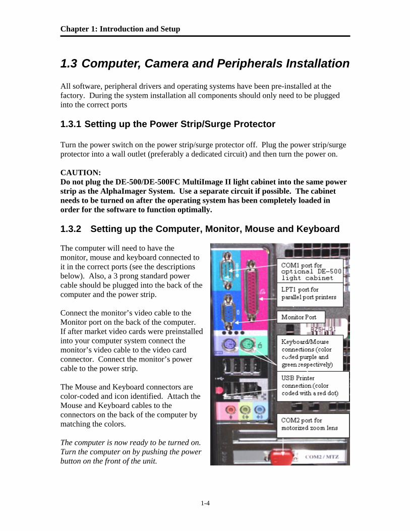
1.3 Computer, Camera and Peripherals Installation All software, peripheral drivers and operating systems have been pre-installed at the factory. During the system installation all components should only need to be plugged into the correct ports 1.3.1 Setting up the Power Strip/Surge Protector Turn the power switch on the power strip/surge protector off. Plug the power strip/surge protector into a wall outlet (preferably a dedicated circuit) and then turn the power on. CAUTION: Do not plug the DE-500/DE-500FC MultiImage II light cabinet into the same power strip as the AlphaImager System. Use a separate circuit if possible. The cabinet needs to be turned on after the operating system has been completely loaded in order for the software to function optimally. 1.3.2 Setting up the Computer, Monitor, Mouse and Keyboard The computer will need to have the monitor, mouse and keyboard connected to it in the correct ports (see the descriptions below). Also, a 3 prong standard power cable should be plugged into the back of the computer and the power strip. Connect the monitor’s video cable to the Monitor port on the back of the computer. If after market video cards were preinstalled into your computer system connect the monitor’s video cable to the video card connector. Connect the monitor’s power cable to the power strip. The Mouse and Keyboard connectors are color-coded and icon identified. Attach the Mouse and Keyboard cables to the connectors on the back of the computer by matching the colors. The computer is now ready to be turned on. Turn the computer on by pushing the power button on the front of the unit.
Alpha Innotech User’s Manual, version 4
1-5
1.3.3 Camera Installation
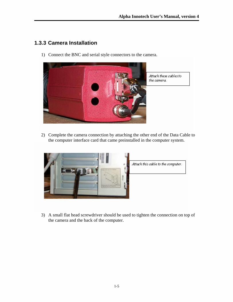
1) Connect the BNC and serial style connectors to the camera.
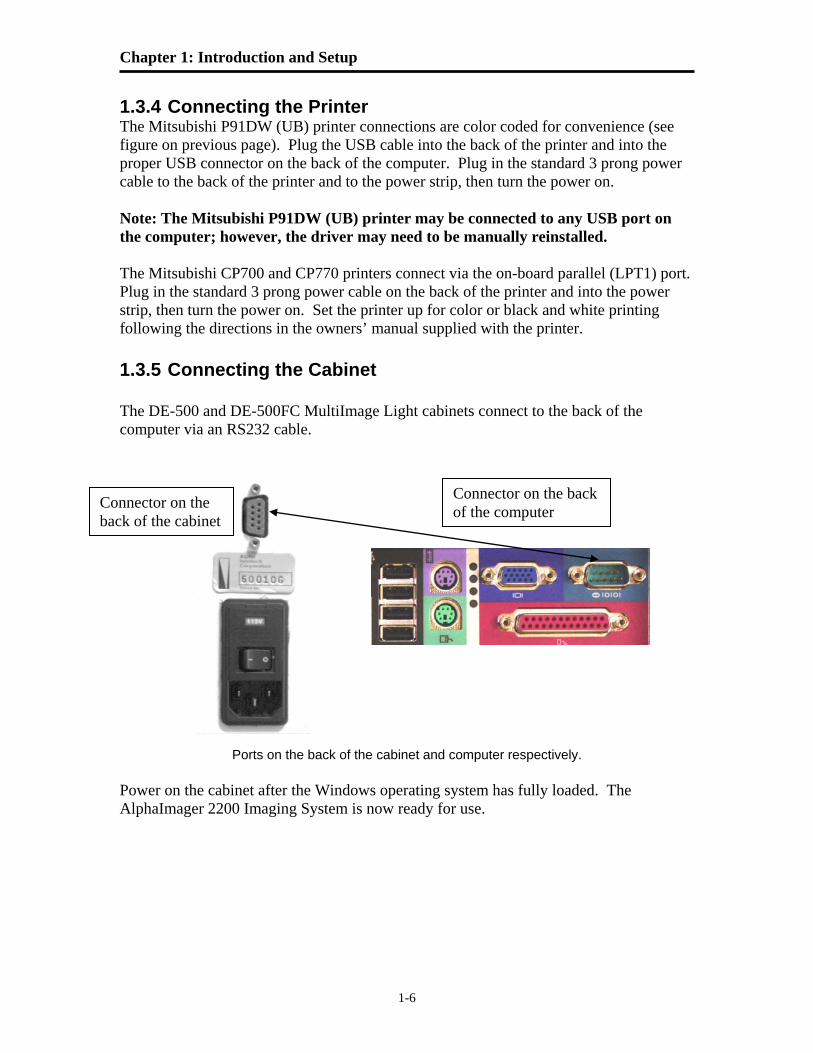
2) Complete the camera connection by attaching the other end of the Data Cable to
the computer interface card that came preinstalled in the computer system.
3) A small flat head screwdriver should be used to tighten the connection on top of
the camera and the back of the computer.
Chapter 1: Introduction and Setup
1-6
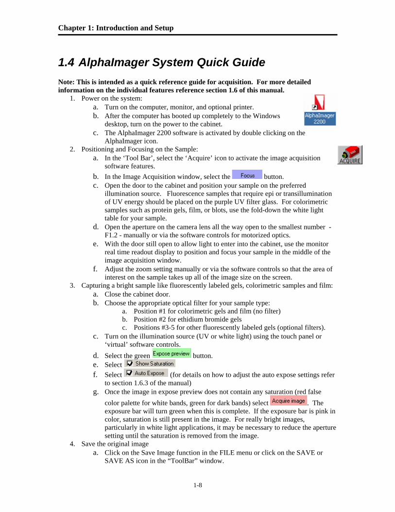
1.3.4 Connecting the Printer The Mitsubishi P91DW (UB) printer connections are color coded for convenience (see figure on previous page). Plug the USB cable into the back of the printer and into the proper USB connector on the back of the computer. Plug in the standard 3 prong power cable to the back of the printer and to the power strip, then turn the power on. Note: The Mitsubishi P91DW (UB) printer may be connected to any USB port on the computer; however, the driver may need to be manually reinstalled. The Mitsubishi CP700 and CP770 printers connect via the on-board parallel (LPT1) port. Plug in the standard 3 prong power cable on the back of the printer and into the power strip, then turn the power on. Set the printer up for color or black and white printing following the directions in the owners’ manual supplied with the printer. 1.3.5 Connecting the Cabinet The DE-500 and DE-500FC MultiImage Light cabinets connect to the back of the computer via an RS232 cable.
Ports on the back of the cabinet and computer respectively.
Power on the cabinet after the Windows operating system has fully loaded. The AlphaImager 2200 Imaging System is now ready for use.
Connector on the back of the cabinet
Connector on the back of the computer

Alpha Innotech User’s Manual, version 4
1-7
1.3.6 Starting AlphaImager System with AlphaEaseFC software To start the AlphaImager 2200 Imaging System software from Windows, double-click the AlphaImager System icon on the windows desktop.
Chapter 1: Introduction and Setup
1-8
1.4 AlphaImager System Quick Guide Note: This is intended as a quick reference guide for acquisition. For more detailed information on the individual features reference section 1.6 of this manual.
1. Power on the system: a. Turn on the computer, monitor, and optional printer. b. After the computer has booted up completely to the Windows
desktop, turn on the power to the cabinet. c. The AlphaImager 2200 software is activated by double clicking on the
AlphaImager icon. 2. Positioning and Focusing on the Sample:
a. In the ‘Tool Bar’, select the ‘Acquire’ icon to activate the image acquisition software features.
b. In the Image Acquisition window, select the button. c. Open the door to the cabinet and position your sample on the preferred
illumination source. Fluorescence samples that require epi or transillumination of UV energy should be placed on the purple UV filter glass. For colorimetric samples such as protein gels, film, or blots, use the fold-down the white light table for your sample.
d. Open the aperture on the camera lens all the way open to the smallest number - F1.2 - manually or via the software controls for motorized optics.
e. With the door still open to allow light to enter into the cabinet, use the monitor real time readout display to position and focus your sample in the middle of the image acquisition window.
f. Adjust the zoom setting manually or via the software controls so that the area of interest on the sample takes up all of the image size on the screen.
3. Capturing a bright sample like fluorescently labeled gels, colorimetric samples and film: a. Close the cabinet door. b. Choose the appropriate optical filter for your sample type:
a. Position #1 for colorimetric gels and film (no filter) b. Position #2 for ethidium bromide gels c. Positions #3-5 for other fluorescently labeled gels (optional filters).
c. Turn on the illumination source (UV or white light) using the touch panel or ‘virtual’ software controls.
d. Select the green button. e. Select f. Select (for details on how to adjust the auto expose settings refer
to section 1.6.3 of the manual) g. Once the image in expose preview does not contain any saturation (red false
color palette for white bands, green for dark bands) select . The exposure bar will turn green when this is complete. If the exposure bar is pink in color, saturation is still present in the image. For really bright images, particularly in white light applications, it may be necessary to reduce the aperture setting until the saturation is removed from the image.
4. Save the original image a. Click on the Save Image function in the FILE menu or click on the SAVE or
SAVE AS icon in the “ToolBar” window.
Alpha Innotech User’s Manual, version 4
1-9
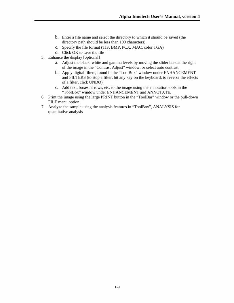
b. Enter a file name and select the directory to which it should be saved (the directory path should be less than 100 characters).
c. Specify the file format (TIF, BMP, PCX, MAC, color TGA) d. Click OK to save the file
5. Enhance the display [optional] a. Adjust the black, white and gamma levels by moving the slider bars at the right
of the image in the “Contrast Adjust” window, or select auto contrast. b. Apply digital filters, found in the “ToolBox” window under ENHANCEMENT
and FILTERS (to stop a filter, hit any key on the keyboard; to reverse the effects of a filter, click UNDO).
c. Add text, boxes, arrows, etc. to the image using the annotation tools in the “ToolBox” window under ENHANCEMENT and ANNOTATE.
6. Print the image using the large PRINT button in the “ToolBar” window or the pull-down FILE menu option
7. Analyze the sample using the analysis features in “ToolBox”, ANALYSIS for quantitative analysis
Chapter 1: Introduction and Setup
1-10
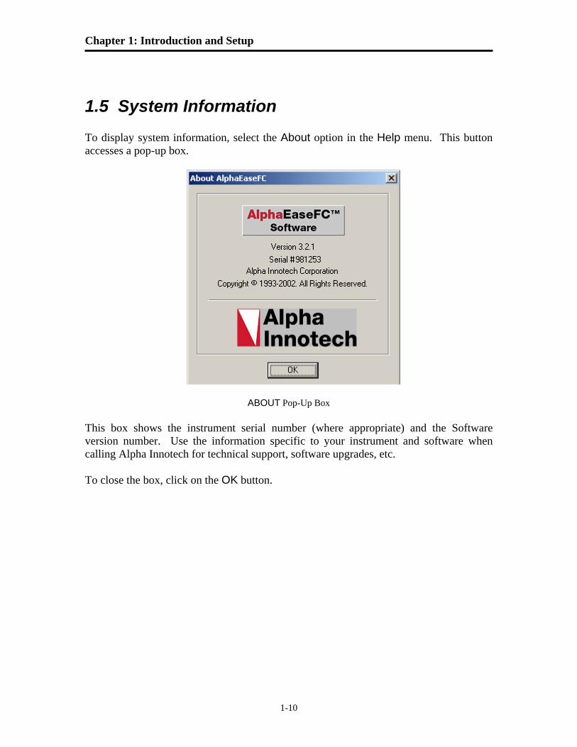
1.5 System Information To display system information, select the About option in the Help menu. This button accesses a pop-up box.
ABOUT Pop-Up Box This box shows the instrument serial number (where appropriate) and the Software version number. Use the information specific to your instrument and software when calling Alpha Innotech for technical support, software upgrades, etc. To close the box, click on the OK button.
Alpha Innotech User’s Manual, version 4
1-11
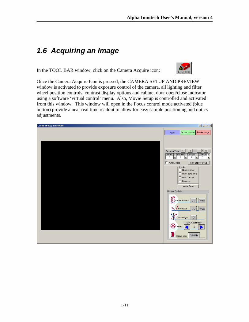
1.6 Acquiring an Image In the TOOL BAR window, click on the Camera Acquire icon: Once the Camera Acquire Icon is pressed, the CAMERA SETUP AND PREVIEW window is activated to provide exposure control of the camera, all lighting and filter wheel position controls, contrast display options and cabinet door open/close indicator using a software ‘virtual control’ menu. Also, Movie Setup is controlled and activated from this window. This window will open in the Focus control mode activated (blue button) provide a near real time readout to allow for easy sample positioning and optics adjustments.
Chapter 1: Introduction and Setup
1-12
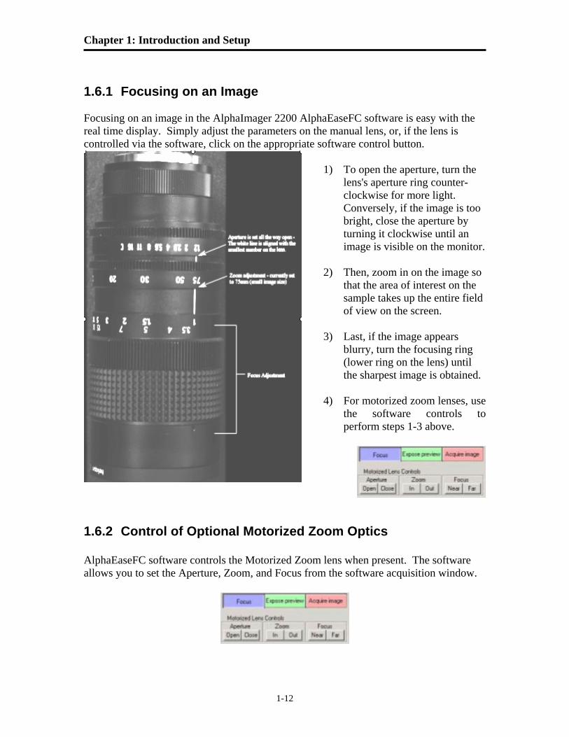
1.6.1 Focusing on an Image Focusing on an image in the AlphaImager 2200 AlphaEaseFC software is easy with the real time display. Simply adjust the parameters on the manual lens, or, if the lens is controlled via the software, click on the appropriate software control button.
1) To open the aperture, turn the
lens's aperture ring counter-clockwise for more light. Conversely, if the image is too bright, close the aperture by turning it clockwise until an image is visible on the monitor.
2) Then, zoom in on the image so
that the area of interest on the sample takes up the entire field of view on the screen.
3) Last, if the image appears
blurry, turn the focusing ring (lower ring on the lens) until the sharpest image is obtained.
4) For motorized zoom lenses, use
the software controls to perform steps 1-3 above.
1.6.2 Control of Optional Motorized Zoom Optics AlphaEaseFC software controls the Motorized Zoom lens when present. The software allows you to set the Aperture, Zoom, and Focus from the software acquisition window.
Alpha Innotech User’s Manual, version 4
1-13
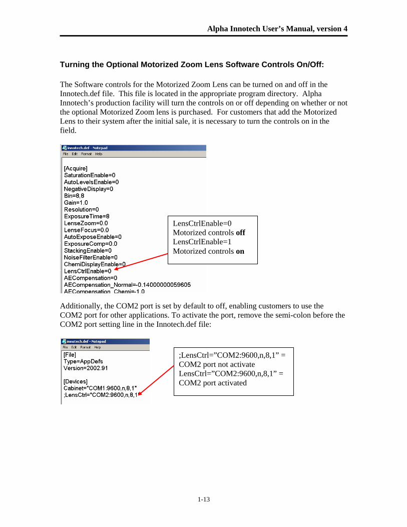
Turning the Optional Motorized Zoom Lens Software Controls On/Off: The Software controls for the Motorized Zoom Lens can be turned on and off in the Innotech.def file. This file is located in the appropriate program directory. Alpha Innotech’s production facility will turn the controls on or off depending on whether or not the optional Motorized Zoom lens is purchased. For customers that add the Motorized Lens to their system after the initial sale, it is necessary to turn the controls on in the field.
Additionally, the COM2 port is set by default to off, enabling customers to use the COM2 port for other applications. To activate the port, remove the semi-colon before the COM2 port setting line in the Innotech.def file:
LensCtrlEnable=0 Motorized controls off LensCtrlEnable=1 Motorized controls on
;LensCtrl=”COM2:9600,n,8,1” = COM2 port not activate LensCtrl=”COM2:9600,n,8,1” = COM2 port activated
Chapter 1: Introduction and Setup
1-14
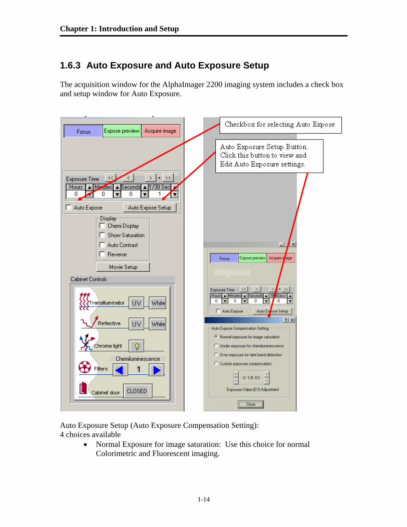
1.6.3 Auto Exposure and Auto Exposure Setup The acquisition window for the AlphaImager 2200 imaging system includes a check box and setup window for Auto Exposure.
Auto Exposure Setup (Auto Exposure Compensation Setting): 4 choices available
• Normal Exposure for image saturation: Use this choice for normal Colorimetric and Fluorescent imaging.
Alpha Innotech User’s Manual, version 4
1-15
• Under Exposure for chemilumenescence • Over Exposure for faint band detection. • Custom Exposure Compensation: user definable Exposure Value (EV).
The up/down arrows allow the user to change the EV value by whole units (left up/down arrows) or by 1/8th (right up/down arrows). Auto Exposure works in both “Expose Preview” and “Acquire Image” modes. As the software calculates the correct exposure time you will see the status bar change from red to yellow and then to green. When it reaches green the software has achieved the correct exposure time. If the bar turns pink, this is an indication that there is saturated pixels in the image area at the exposure time calculated. In Acquire Image mode the image will be acquired when the bar turns green. In Expose Preview mode the software will continue exposing over and over at that exposure time until a different mode is selected. If “Acquire Image” is selected after the software has achieved the correct exposure time in Expose Preview the software will begin acquiring at the last exposure time calculated in Expose Preview—it does not start the calculation over from scratch.
Chapter 1: Introduction and Setup
1-16
1.6.4 Cabinet Controls - Activating the Light Source and Selecting a Filter Use the mouse to click on the desired light source in the ‘virtual’ cabinet control interface or you can use the controls on the cabinet itself. Both mechanical and software controls are linked and communicate display setting selections. Note: There is a slight delay when the button is depressed until the light source is fully activated. Standard lighting choices include: Transillumination White: For protein gels, autorads, film, plates, flasks Transillumination UV: For fluorescent gels such EtBr, SYPRO Red, etc. Reflective White: For colorimetric blots and membranes
Reflective UV (optional) For SYBR green, TLC plates, and Chemifluorescence
ChromaLight (optional) For GFP, Fluorescein, SYBR green
You can also select your FILTER to correspond with your sample staining. The options include: Filter Position #1: no filter
Filter Position #2: Ethidium Bromide, colorimetric stains, film, SYPRO Orange (595nm)
Filter Position #3 (optional): SYBR green (557nm) Filter Position #4 (optional): Fluorescein, SYBR Gold (520nm) Filter Position #5 (optional): SYPRO Red, Texas Red (630nm) (optional): Hoechst Blue (460nm) Note: Each Filter has an approximate bandwidth of +/- 40nm to allow for use with other fluorescence stains as they are developed. If you have a custom application, please feel free to contact us directly to explore having a custom filter designed for your application.
Alpha Innotech User’s Manual, version 4
1-17
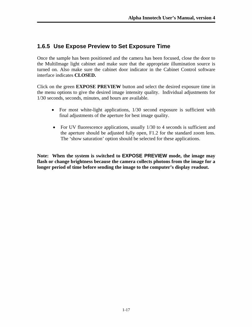
1.6.5 Use Expose Preview to Set Exposure Time Once the sample has been positioned and the camera has been focused, close the door to the MultiImage light cabinet and make sure that the appropriate illumination source is turned on. Also make sure the cabinet door indicator in the Cabinet Control software interface indicates CLOSED. Click on the green EXPOSE PREVIEW button and select the desired exposure time in the menu options to give the desired image intensity quality. Individual adjustments for 1/30 seconds, seconds, minutes, and hours are available.
• For most white-light applications, 1/30 second exposure is sufficient with final adjustments of the aperture for best image quality.
• For UV fluorescence applications, usually 1/30 to 4 seconds is sufficient and
the aperture should be adjusted fully open, F1.2 for the standard zoom lens. The ‘show saturation’ option should be selected for these applications.
Note: When the system is switched to EXPOSE PREVIEW mode, the image may flash or change brightness because the camera collects photons from the image for a longer period of time before sending the image to the computer’s display readout.
Chapter 1: Introduction and Setup
1-18
1.6.6 Optimizing the Gray Scale for Saturation and Contrast
Displays
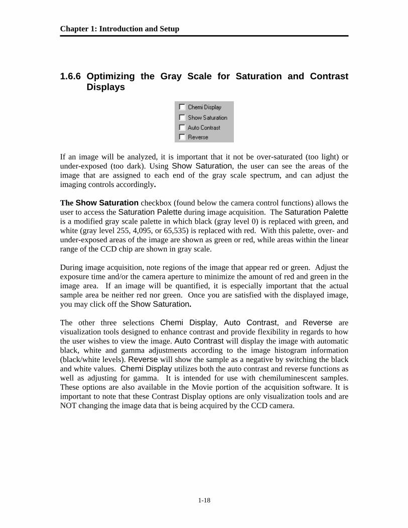
If an image will be analyzed, it is important that it not be over-saturated (too light) or under-exposed (too dark). Using Show Saturation, the user can see the areas of the image that are assigned to each end of the gray scale spectrum, and can adjust the imaging controls accordingly. The Show Saturation checkbox (found below the camera control functions) allows the user to access the Saturation Palette during image acquisition. The Saturation Palette is a modified gray scale palette in which black (gray level 0) is replaced with green, and white (gray level 255, 4,095, or 65,535) is replaced with red. With this palette, over- and under-exposed areas of the image are shown as green or red, while areas within the linear range of the CCD chip are shown in gray scale. During image acquisition, note regions of the image that appear red or green. Adjust the exposure time and/or the camera aperture to minimize the amount of red and green in the image area. If an image will be quantified, it is especially important that the actual sample area be neither red nor green. Once you are satisfied with the displayed image, you may click off the Show Saturation. The other three selections Chemi Display, Auto Contrast, and Reverse are visualization tools designed to enhance contrast and provide flexibility in regards to how the user wishes to view the image. Auto Contrast will display the image with automatic black, white and gamma adjustments according to the image histogram information (black/white levels). Reverse will show the sample as a negative by switching the black and white values. Chemi Display utilizes both the auto contrast and reverse functions as well as adjusting for gamma. It is intended for use with chemiluminescent samples. These options are also available in the Movie portion of the acquisition software. It is important to note that these Contrast Display options are only visualization tools and are NOT changing the image data that is being acquired by the CCD camera.
Alpha Innotech User’s Manual, version 4
1-19
1.6.7 Acquire and Transfer the Image Once the appropriate image is displayed on the screen, click on the red ACQUIRE IMAGE button to capture and transfer the image to the AlphaEaseFC software package for enhancement, archiving, or analysis. The acquired image will be automatically adjusted by a zoom factor based on the resolution setting to display the image optimally. Once a satisfactory image has been captured, we suggest saving it as an original file. Use the Save Image As function in the File menu or click on the Save or Save As Icons.
Chapter 1: Introduction and Setup
1-20
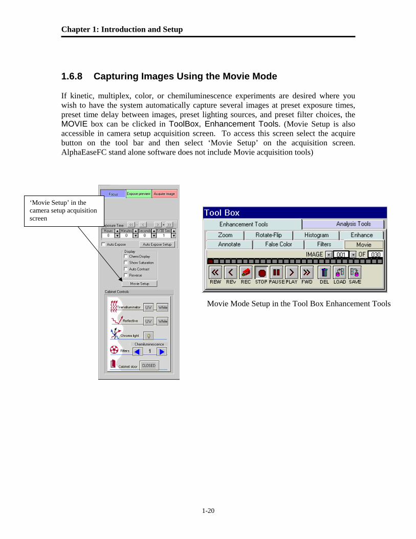
1.6.8 Capturing Images Using the Movie Mode If kinetic, multiplex, color, or chemiluminescence experiments are desired where you wish to have the system automatically capture several images at preset exposure times, preset time delay between images, preset lighting sources, and preset filter choices, the MOVIE box can be clicked in ToolBox, Enhancement Tools. (Movie Setup is also accessible in camera setup acquisition screen. To access this screen select the acquire button on the tool bar and then select ‘Movie Setup’ on the acquisition screen. AlphaEaseFC stand alone software does not include Movie acquisition tools)
‘Movie Setup’ in the camera setup acquisition screen
Movie Mode Setup in the Tool Box Enhancement Tools
Alpha Innotech User’s Manual, version 4
1-21
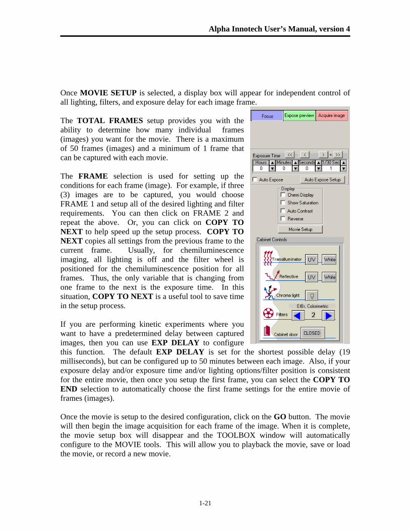
Once MOVIE SETUP is selected, a display box will appear for independent control of all lighting, filters, and exposure delay for each image frame. The TOTAL FRAMES setup provides you with the ability to determine how many individual frames (images) you want for the movie. There is a maximum of 50 frames (images) and a minimum of 1 frame that can be captured with each movie. The FRAME selection is used for setting up the conditions for each frame (image). For example, if three (3) images are to be captured, you would choose FRAME 1 and setup all of the desired lighting and filter requirements. You can then click on FRAME 2 and repeat the above. Or, you can click on COPY TO NEXT to help speed up the setup process. COPY TO NEXT copies all settings from the previous frame to the current frame. Usually, for chemiluminescence imaging, all lighting is off and the filter wheel is positioned for the chemiluminescence position for all frames. Thus, the only variable that is changing from one frame to the next is the exposure time. In this situation, COPY TO NEXT is a useful tool to save time in the setup process. If you are performing kinetic experiments where you want to have a predetermined delay between captured images, then you can use EXP DELAY to configure this function. The default EXP DELAY is set for the shortest possible delay (19 milliseconds), but can be configured up to 50 minutes between each image. Also, if your exposure delay and/or exposure time and/or lighting options/filter position is consistent for the entire movie, then once you setup the first frame, you can select the COPY TO END selection to automatically choose the first frame settings for the entire movie of frames (images). Once the movie is setup to the desired configuration, click on the GO button. The movie will then begin the image acquisition for each frame of the image. When it is complete, the movie setup box will disappear and the TOOLBOX window will automatically configure to the MOVIE tools. This will allow you to playback the movie, save or load the movie, or record a new movie.
Chapter 1: Introduction and Setup
1-22
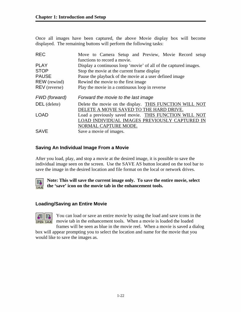
Once all images have been captured, the above Movie display box will become displayed. The remaining buttons will perform the following tasks: REC Move to Camera Setup and Preview, Movie Record setup
functions to record a movie. PLAY Display a continuous loop ‘movie’ of all of the captured images. STOP Stop the movie at the current frame display PAUSE Pause the playback of the movie at a user defined image REW (rewind) Rewind the movie to the first image REV (reverse) Play the movie in a continuous loop in reverse
FWD (forward) Forward the movie to the last image DEL (delete) Delete the movie on the display. THIS FUNCTION WILL NOT
DELETE A MOVIE SAVED TO THE HARD DRIVE. LOAD Load a previously saved movie. THIS FUNCTION WILL NOT
LOAD INDIVIDUAL IMAGES PREVIOUSLY CAPTURED IN NORMAL CAPTURE MODE.
SAVE Save a movie of images. Saving An Individual Image From a Movie After you load, play, and stop a movie at the desired image, it is possible to save the individual image seen on the screen. Use the SAVE AS button located on the tool bar to save the image in the desired location and file format on the local or network drives.
Note: This will save the current image only. To save the entire movie, select the ‘save’ icon on the movie tab in the enhancement tools.
Loading/Saving an Entire Movie
You can load or save an entire movie by using the load and save icons in the movie tab in the enhancement tools. When a movie is loaded the loaded frames will be seen as blue in the movie reel. When a movie is saved a dialog
box will appear prompting you to select the location and name for the movie that you would like to save the images as.
Alpha Innotech User’s Manual, version 4
1-23
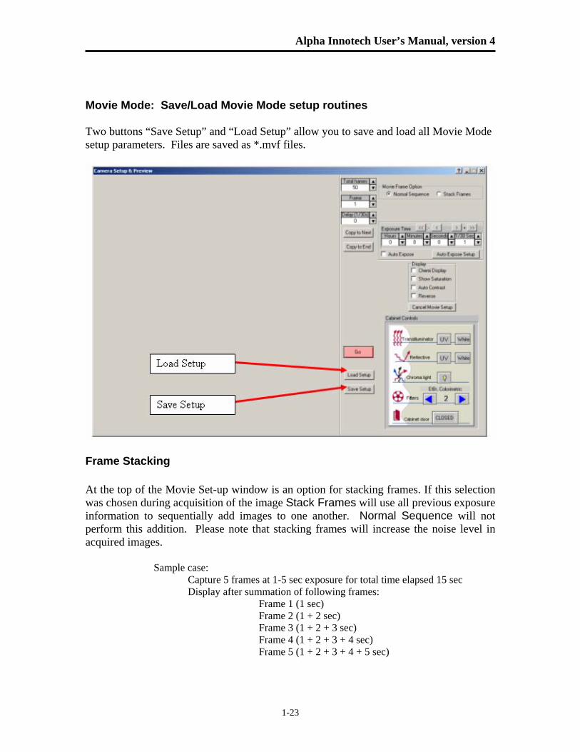
Movie Mode: Save/Load Movie Mode setup routines Two buttons “Save Setup” and “Load Setup” allow you to save and load all Movie Mode setup parameters. Files are saved as *.mvf files.
Frame Stacking At the top of the Movie Set-up window is an option for stacking frames. If this selection was chosen during acquisition of the image Stack Frames will use all previous exposure information to sequentially add images to one another. Normal Sequence will not perform this addition. Please note that stacking frames will increase the noise level in acquired images. Sample case: Capture 5 frames at 1-5 sec exposure for total time elapsed 15 sec Display after summation of following frames:
Frame 1 (1 sec) Frame 2 (1 + 2 sec) Frame 3 (1 + 2 + 3 sec) Frame 4 (1 + 2 + 3 + 4 sec)
Frame 5 (1 + 2 + 3 + 4 + 5 sec)
Chapter 1: Introduction and Setup
1-24
Capturing a Color Image Using the Movie Function A color image can be generated by acquiring three images each taken with a red, green and blue emission filter. Once saved, these images are then combined in the Overlay pull down menu. Open the image captured with each of the three filters as instructed and a RGB (red, green, blue) true color image will be generated. For color imaging, you will need to the following optional filters:
Red Filter SYPRO Red Filter
Blue Filter Hoechst Blue Filter
Green Filter SYBR Green Filter
Note: For multiplexing with 2 different fluorescent stains, you will need the optional AIC filters designed for each stain.

Alpha Innotech User’s Manual, version 4
1-25
BLANK PAGE

Chapter 1: Introduction and Setup
1-26
BLANK PAGE
Chapter 2: Getting Started – Basic Imaging Functions
2-1
Chapter 2: Getting Started - Basic Imaging Functions
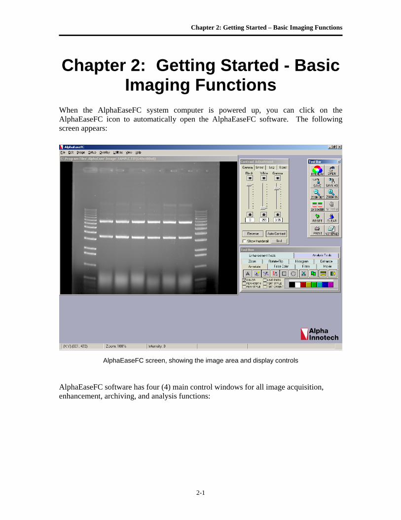
When the AlphaEaseFC system computer is powered up, you can click on the AlphaEaseFC icon to automatically open the AlphaEaseFC software. The following screen appears:
AlphaEaseFC screen, showing the image area and display controls AlphaEaseFC software has four (4) main control windows for all image acquisition, enhancement, archiving, and analysis functions:
Alpha Innotech User’s Manual, version 4
2-2
2.1 Contrast Adjustment The Contrast Adjustment window allows for the best visualization possible of a sample utilizing the black, white, and gamma adjustments, as well as, image reverse and auto contrast.
The image on the screen is made up of picture elements (pixels) in an array. Each pixel is assigned a brightness (or a gray scale value) level between black and white. A very bright image has most of its pixels registering high gray level values and conversely, a very dark image has most pixels registering low gray level values (approaching zero). The distribution of these gray values to the image is determined by the Contrast Adjustment Controls. These controls regulate the Black level, White level, and Gamma setting (brightness linearity), allowing adjustment of the display to obtain the best image possible. Note: These enhancement features modify the image display on the monitor only, and do not change the original quantitative data. AlphaEaseFC software can also import RGB color images. The AlphaEaseFC Software automatically detects this process and the Contrast Adjustment tools are configured for color image adjustments. An image can be enhanced using these tools and then saved as a Modified file for publications. However, to preserve the original image information, it is recommended that the file be saved as a different file name when using the save modified. Using the Contrast Adjustment Tools for Grayscale Images There are three sliding scales found in the image control area to the right of the image. Below each scale is a box displaying a number that corresponds to the position of the slider. By adjusting these sliding scales, the image display can be optimized.
Chapter 2: Getting Started – Basic Imaging Functions
2-3
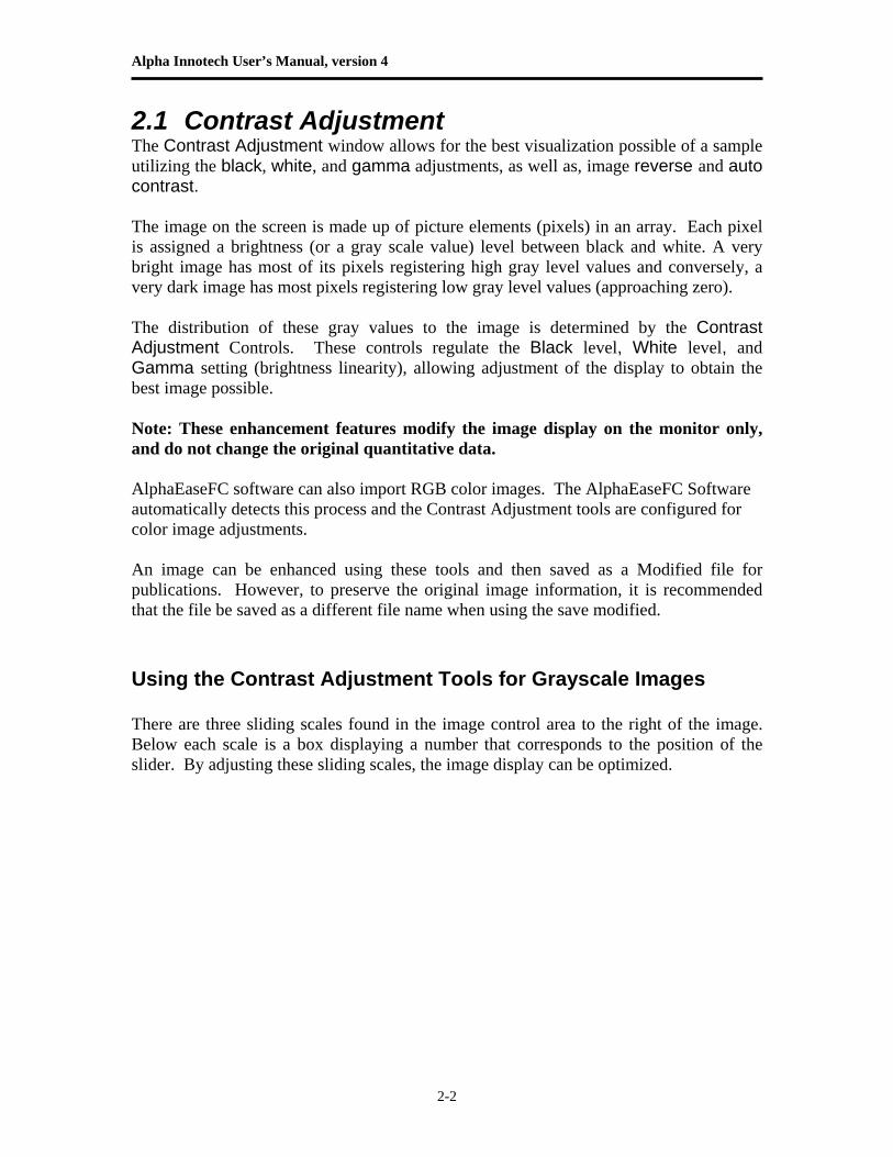
Imaging Display Tools: Black Level, White Level, Gamma Setting with B/W/G, Linear, Log, and Equalize options
To adjust any of these settings, place the cursor on the slider. Click and hold down the left mouse button while dragging the slider to a new setting. As the slider is moved along the scale, the image display is updated, along with the change in numeric value. The arrows above and below the scale bars can also be clicked to change the settings in single unit increments, or, the user may type in a specific unit.
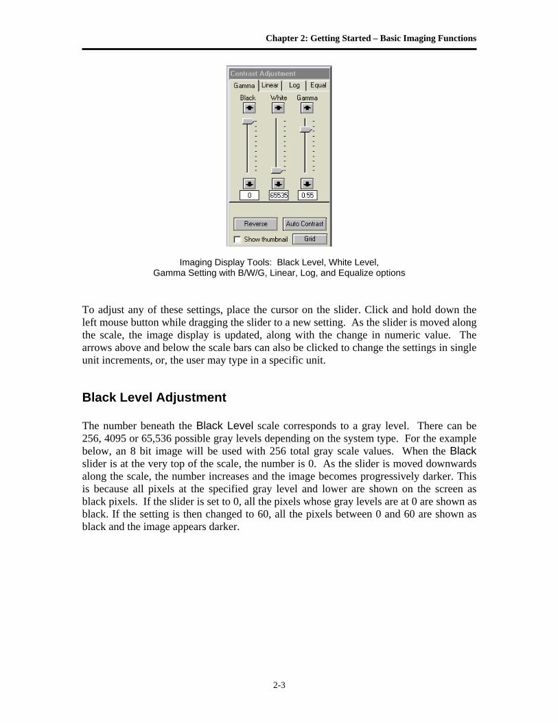
Black Level Adjustment The number beneath the Black Level scale corresponds to a gray level. There can be 256, 4095 or 65,536 possible gray levels depending on the system type. For the example below, an 8 bit image will be used with 256 total gray scale values. When the Black slider is at the very top of the scale, the number is 0. As the slider is moved downwards along the scale, the number increases and the image becomes progressively darker. This is because all pixels at the specified gray level and lower are shown on the screen as black pixels. If the slider is set to 0, all the pixels whose gray levels are at 0 are shown as black. If the setting is then changed to 60, all the pixels between 0 and 60 are shown as black and the image appears darker.
Alpha Innotech User’s Manual, version 4
2-4
Black Level set at 0 Black Level set at 60
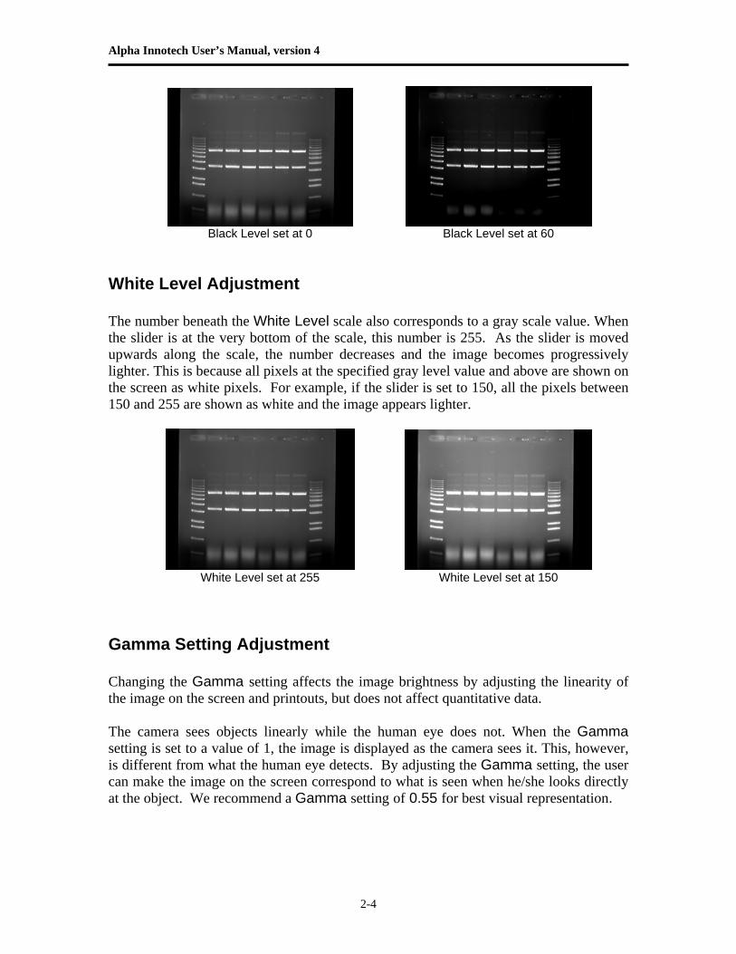
White Level Adjustment The number beneath the White Level scale also corresponds to a gray scale value. When the slider is at the very bottom of the scale, this number is 255. As the slider is moved upwards along the scale, the number decreases and the image becomes progressively lighter. This is because all pixels at the specified gray level value and above are shown on the screen as white pixels. For example, if the slider is set to 150, all the pixels between 150 and 255 are shown as white and the image appears lighter.
White Level set at 255 White Level set at 150 Gamma Setting Adjustment Changing the Gamma setting affects the image brightness by adjusting the linearity of the image on the screen and printouts, but does not affect quantitative data. The camera sees objects linearly while the human eye does not. When the Gamma setting is set to a value of 1, the image is displayed as the camera sees it. This, however, is different from what the human eye detects. By adjusting the Gamma setting, the user can make the image on the screen correspond to what is seen when he/she looks directly at the object. We recommend a Gamma setting of 0.55 for best visual representation.
Chapter 2: Getting Started – Basic Imaging Functions
2-5
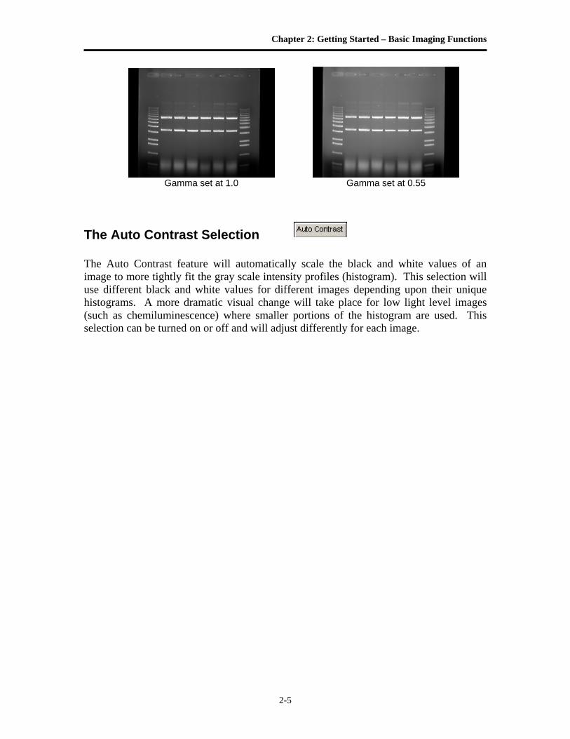
Gamma set at 1.0 Gamma set at 0.55 The Auto Contrast Selection The Auto Contrast feature will automatically scale the black and white values of an image to more tightly fit the gray scale intensity profiles (histogram). This selection will use different black and white values for different images depending upon their unique histograms. A more dramatic visual change will take place for low light level images (such as chemiluminescence) where smaller portions of the histogram are used. This selection can be turned on or off and will adjust differently for each image.
Alpha Innotech User’s Manual, version 4
2-6
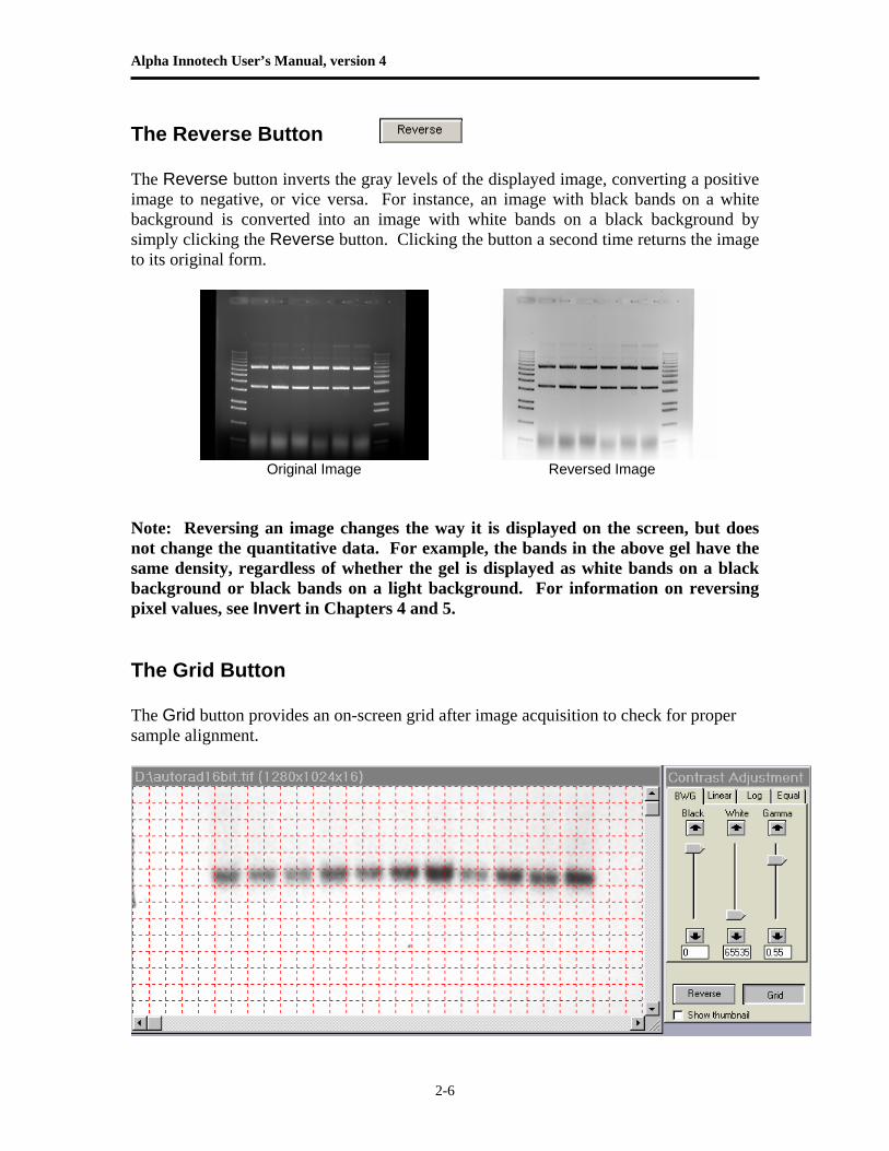
The Reverse Button The Reverse button inverts the gray levels of the displayed image, converting a positive image to negative, or vice versa. For instance, an image with black bands on a white background is converted into an image with white bands on a black background by simply clicking the Reverse button. Clicking the button a second time returns the image to its original form.
Original Image Reversed Image Note: Reversing an image changes the way it is displayed on the screen, but does not change the quantitative data. For example, the bands in the above gel have the same density, regardless of whether the gel is displayed as white bands on a black background or black bands on a light background. For information on reversing pixel values, see Invert in Chapters 4 and 5. The Grid Button The Grid button provides an on-screen grid after image acquisition to check for proper sample alignment.
Chapter 2: Getting Started – Basic Imaging Functions
2-7
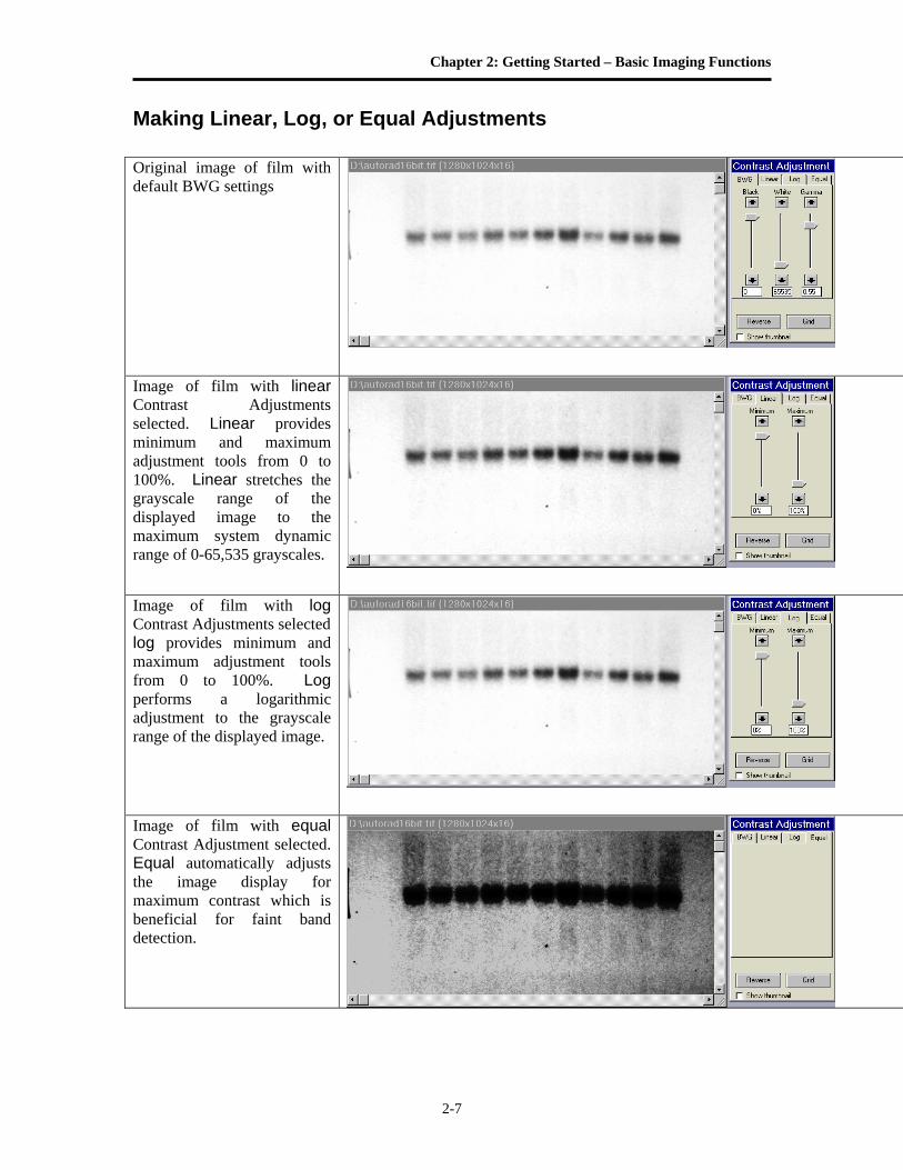
Making Linear, Log, or Equal Adjustments Original image of film with default BWG settings
Image of film with linear Contrast Adjustments selected. Linear provides minimum and maximum adjustment tools from 0 to 100%. Linear stretches the grayscale range of the displayed image to the maximum system dynamic range of 0-65,535 grayscales.
Image of film with log Contrast Adjustments selected log provides minimum and maximum adjustment tools from 0 to 100%. Log performs a logarithmic adjustment to the grayscale range of the displayed image.
Image of film with equal Contrast Adjustment selected. Equal automatically adjusts the image display for maximum contrast which is beneficial for faint band detection.
Alpha Innotech User’s Manual, version 4
2-8
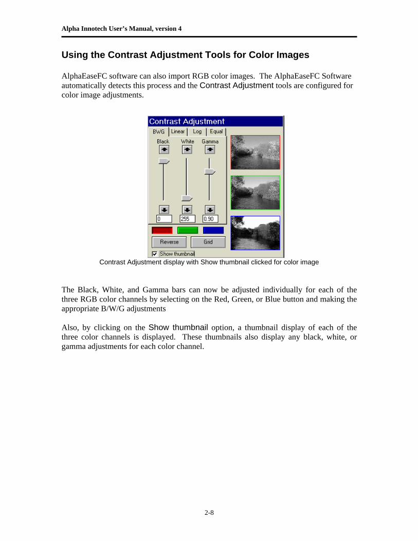
Using the Contrast Adjustment Tools for Color Images AlphaEaseFC software can also import RGB color images. The AlphaEaseFC Software automatically detects this process and the Contrast Adjustment tools are configured for color image adjustments.
Contrast Adjustment display with Show thumbnail clicked for color image The Black, White, and Gamma bars can now be adjusted individually for each of the three RGB color channels by selecting on the Red, Green, or Blue button and making the appropriate B/W/G adjustments Also, by clicking on the Show thumbnail option, a thumbnail display of each of the three color channels is displayed. These thumbnails also display any black, white, or gamma adjustments for each color channel.
Chapter 2: Getting Started – Basic Imaging Functions
2-9
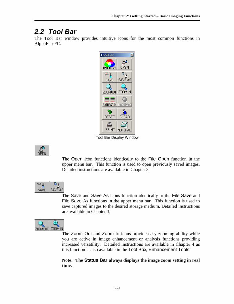
2.2 Tool Bar The Tool Bar window provides intuitive icons for the most common functions in AlphaEaseFC.
Tool Bar Display Window
The Open icon functions identically to the File Open function in the upper menu bar. This function is used to open previously saved images. Detailed instructions are available in Chapter 3.
The Save and Save As icons function identically to the File Save and File Save As functions in the upper menu bar. This function is used to save captured images to the desired storage medium. Detailed instructions are available in Chapter 3.
The Zoom Out and Zoom In icons provide easy zooming ability while you are active in image enhancement or analysis functions providing increased versatility. Detailed instructions are available in Chapter 4 as this function is also available in the Tool Box, Enhancement Tools. Note: The Status Bar always displays the image zoom setting in real time.
Alpha Innotech User’s Manual, version 4
2-10
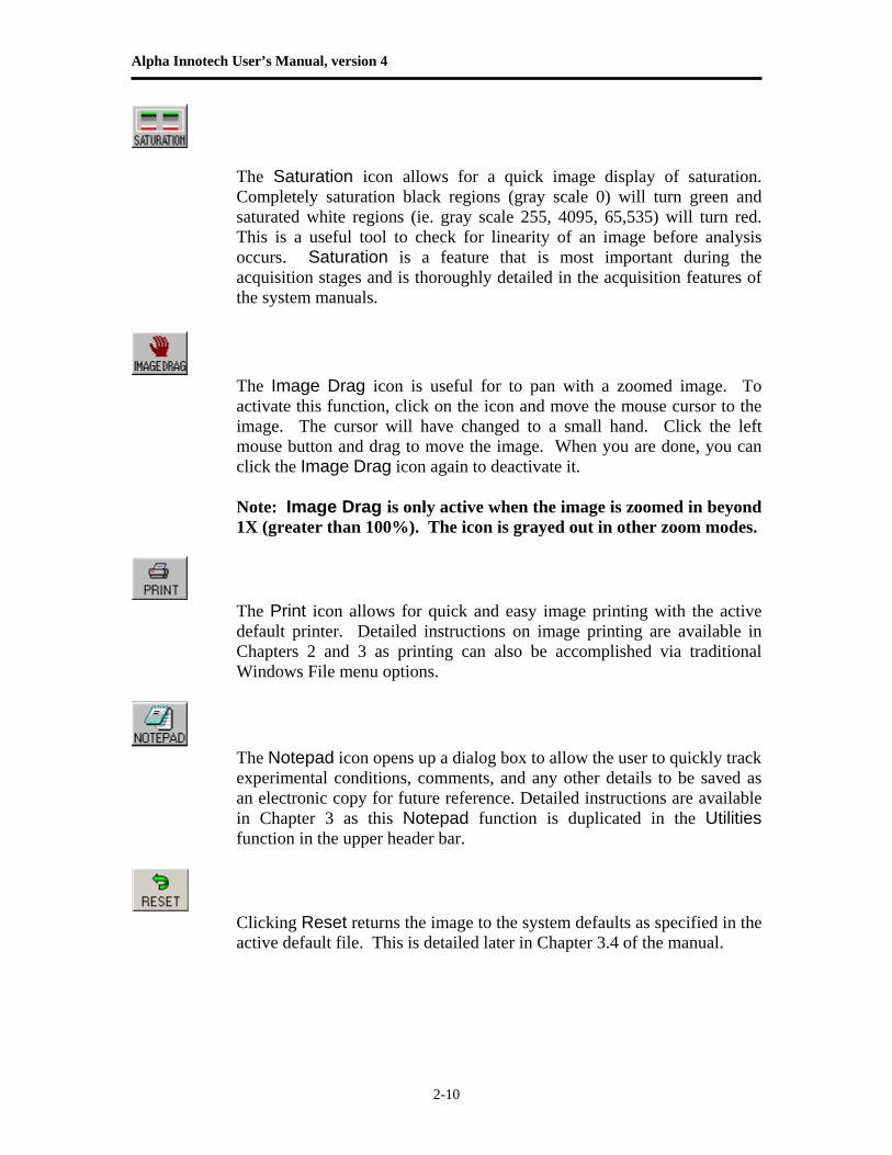
The Saturation icon allows for a quick image display of saturation. Completely saturation black regions (gray scale 0) will turn green and saturated white regions (ie. gray scale 255, 4095, 65,535) will turn red. This is a useful tool to check for linearity of an image before analysis occurs. Saturation is a feature that is most important during the acquisition stages and is thoroughly detailed in the acquisition features of the system manuals.
The Image Drag icon is useful for to pan with a zoomed image. To activate this function, click on the icon and move the mouse cursor to the image. The cursor will have changed to a small hand. Click the left mouse button and drag to move the image. When you are done, you can click the Image Drag icon again to deactivate it. Note: Image Drag is only active when the image is zoomed in beyond 1X (greater than 100%). The icon is grayed out in other zoom modes.
The Print icon allows for quick and easy image printing with the active default printer. Detailed instructions on image printing are available in Chapters 2 and 3 as printing can also be accomplished via traditional Windows File menu options.
The Notepad icon opens up a dialog box to allow the user to quickly track experimental conditions, comments, and any other details to be saved as an electronic copy for future reference. Detailed instructions are available in Chapter 3 as this Notepad function is duplicated in the Utilities function in the upper header bar.
Clicking Reset returns the image to the system defaults as specified in the active default file. This is detailed later in Chapter 3.4 of the manual.
Chapter 2: Getting Started – Basic Imaging Functions
2-11
Clear removes any overlays currently displayed on the image. This function can be useful if annotations or other displays obscure parts of the image.
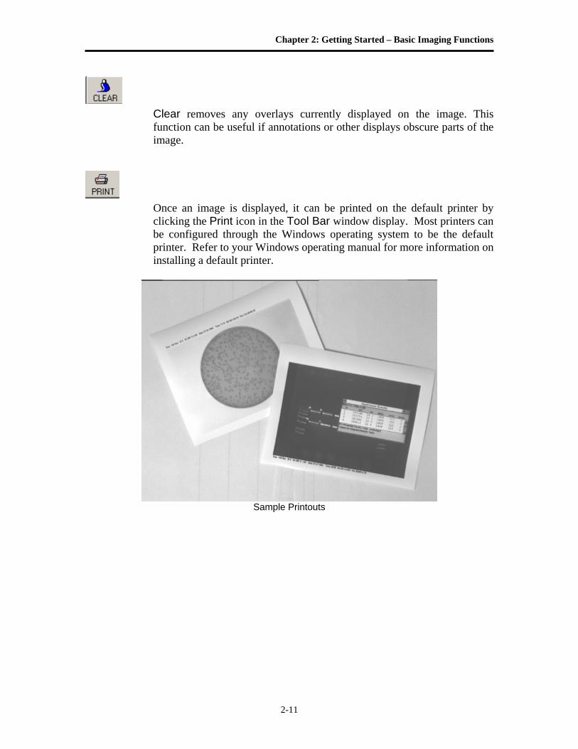
Once an image is displayed, it can be printed on the default printer by clicking the Print icon in the Tool Bar window display. Most printers can be configured through the Windows operating system to be the default printer. Refer to your Windows operating manual for more information on installing a default printer.
Sample Printouts
Alpha Innotech User’s Manual, version 4
2-12
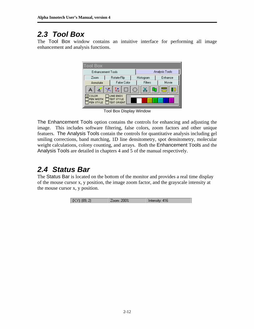
2.3 Tool Box The Tool Box window contains an intuitive interface for performing all image enhancement and analysis functions.
Tool Box Display Window The Enhancement Tools option contains the controls for enhancing and adjusting the image. This includes software filtering, false colors, zoom factors and other unique featuers. The Analysis Tools contain the controls for quantitative analysis including gel smiling corrections, band matching, 1D line densitometry, spot densitometry, molecular weight calculations, colony counting, and arrays. Both the Enhancement Tools and the Analysis Tools are detailed in chapters 4 and 5 of the manual respectively. 2.4 Status Bar The Status Bar is located on the bottom of the monitor and provides a real time display of the mouse cursor x, y position, the image zoom factor, and the grayscale intensity at the mouse cursor x, y position.

Chapter 2: Getting Started – Basic Imaging Functions
2-13
BLANK PAGE

Alpha Innotech User’s Manual, version 4
2-14
BLANK PAGE
Chapter 3: Drop Down Menus
3-1
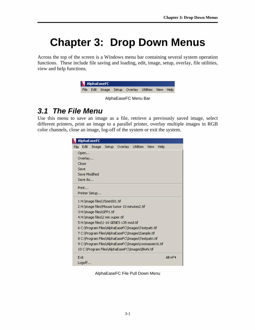
Chapter 3: Drop Down Menus Across the top of the screen is a Windows menu bar containing several system operation functions. These include file saving and loading, edit, image, setup, overlay, file utilities, view and help functions.
AlphaEaseFC Menu Bar
3.1 The File Menu Use this menu to save an image as a file, retrieve a previously saved image, select different printers, print an image to a parallel printer, overlay multiple images in RGB color channels, close an image, log-off of the system or exit the system.
AlphaEaseFC File Pull Down Menu
Alpha Innotech User’s Manual, version 4
3-2
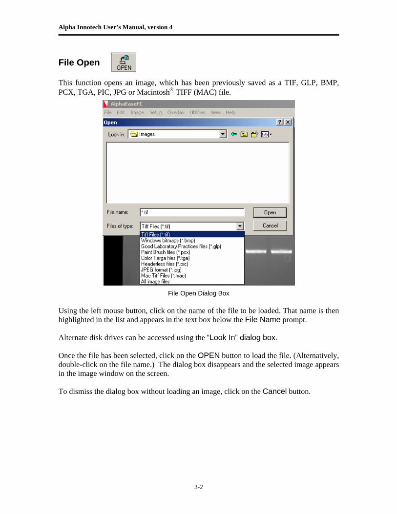
File Open This function opens an image, which has been previously saved as a TIF, GLP, BMP, PCX, TGA, PIC, JPG or Macintosh® TIFF (MAC) file.
File Open Dialog Box
Using the left mouse button, click on the name of the file to be loaded. That name is then highlighted in the list and appears in the text box below the File Name prompt. Alternate disk drives can be accessed using the “Look In” dialog box. Once the file has been selected, click on the OPEN button to load the file. (Alternatively, double-click on the file name.) The dialog box disappears and the selected image appears in the image window on the screen. To dismiss the dialog box without loading an image, click on the Cancel button.
Chapter 3: Drop Down Menus
3-3
File Overlay To superimpose images, use the OVERLAY function under the File menu. This function will display separate multiplexed images or a RGB color image as a compiled image with the appropriate color channel images added together. A simple way to acquire multiple images for this function is to use the Movie Mode function in image acquisition and acquire a series of identical images.
The Overlay Images option allows you to overlay up to three different images with three different color channels. You can select the BROWSE button for each color channel and select the appropriate images to be used for generating a color image. For example, if you have a saved grayscale images of an identical gel taken with a SYPRO red filter for the red stain and a SYBR green filter for the green stain, you can choose these images in the appropriate Red and Green Channels to generate a composite image with the red and green colors mapped onto the compiled image. Note: The images must be the same bit depth and resolution for the software to overlay the images. File Close This function closes the image currently displayed on the screen.
Alpha Innotech User’s Manual, version 4
3-4
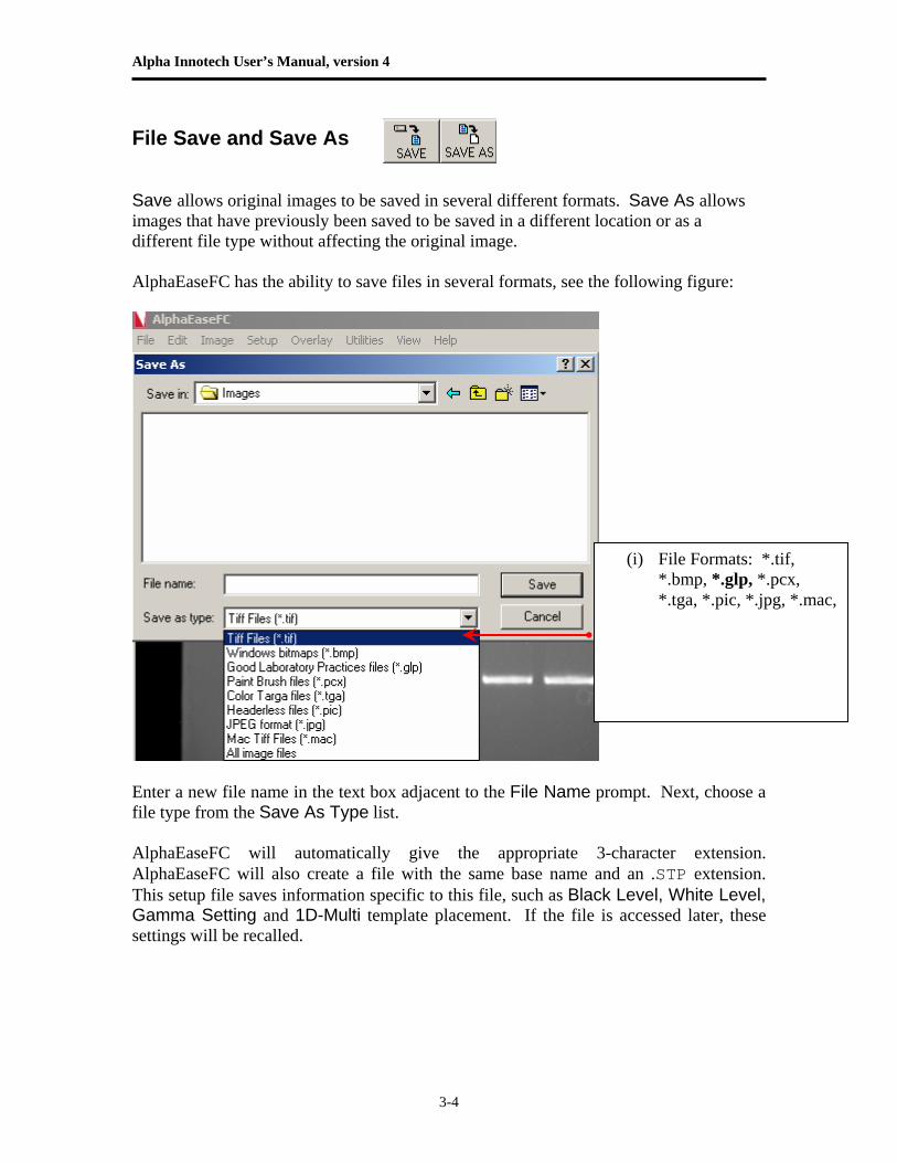
File Save and Save As Save allows original images to be saved in several different formats. Save As allows images that have previously been saved to be saved in a different location or as a different file type without affecting the original image. AlphaEaseFC has the ability to save files in several formats, see the following figure:
Enter a new file name in the text box adjacent to the File Name prompt. Next, choose a file type from the Save As Type list. AlphaEaseFC will automatically give the appropriate 3-character extension. AlphaEaseFC will also create a file with the same base name and an .STP extension. This setup file saves information specific to this file, such as Black Level, White Level, Gamma Setting and 1D-Multi template placement. If the file is accessed later, these settings will be recalled.
(i) File Formats: *.tif, *.bmp, *.glp, *.pcx, *.tga, *.pic, *.jpg, *.mac,
Chapter 3: Drop Down Menus
3-5
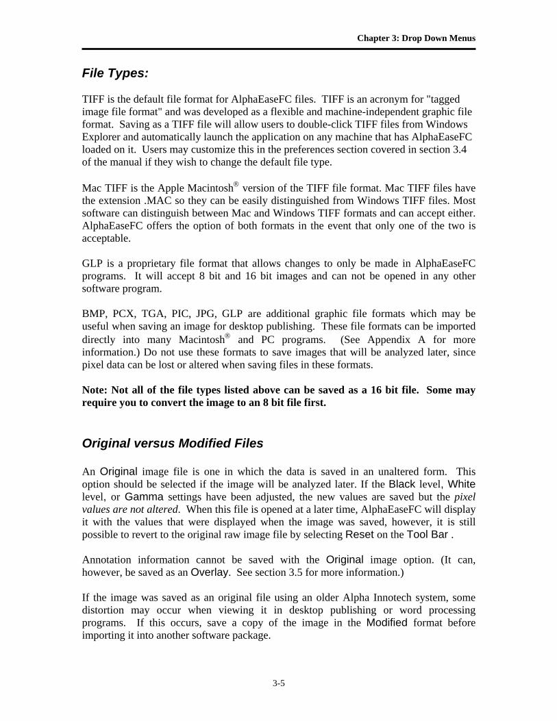
File Types: TIFF is the default file format for AlphaEaseFC files. TIFF is an acronym for "tagged image file format" and was developed as a flexible and machine-independent graphic file format. Saving as a TIFF file will allow users to double-click TIFF files from Windows Explorer and automatically launch the application on any machine that has AlphaEaseFC loaded on it. Users may customize this in the preferences section covered in section 3.4 of the manual if they wish to change the default file type. Mac TIFF is the Apple Macintosh® version of the TIFF file format. Mac TIFF files have the extension .MAC so they can be easily distinguished from Windows TIFF files. Most software can distinguish between Mac and Windows TIFF formats and can accept either. AlphaEaseFC offers the option of both formats in the event that only one of the two is acceptable. GLP is a proprietary file format that allows changes to only be made in AlphaEaseFC programs. It will accept 8 bit and 16 bit images and can not be opened in any other software program. BMP, PCX, TGA, PIC, JPG, GLP are additional graphic file formats which may be useful when saving an image for desktop publishing. These file formats can be imported directly into many Macintosh® and PC programs. (See Appendix A for more information.) Do not use these formats to save images that will be analyzed later, since pixel data can be lost or altered when saving files in these formats. Note: Not all of the file types listed above can be saved as a 16 bit file. Some may require you to convert the image to an 8 bit file first. Original versus Modified Files An Original image file is one in which the data is saved in an unaltered form. This option should be selected if the image will be analyzed later. If the Black level, White level, or Gamma settings have been adjusted, the new values are saved but the pixel values are not altered. When this file is opened at a later time, AlphaEaseFC will display it with the values that were displayed when the image was saved, however, it is still possible to revert to the original raw image file by selecting Reset on the Tool Bar . Annotation information cannot be saved with the Original image option. (It can, however, be saved as an Overlay. See section 3.5 for more information.) If the image was saved as an original file using an older Alpha Innotech system, some distortion may occur when viewing it in desktop publishing or word processing programs. If this occurs, save a copy of the image in the Modified format before importing it into another software package.
Alpha Innotech User’s Manual, version 4
3-6
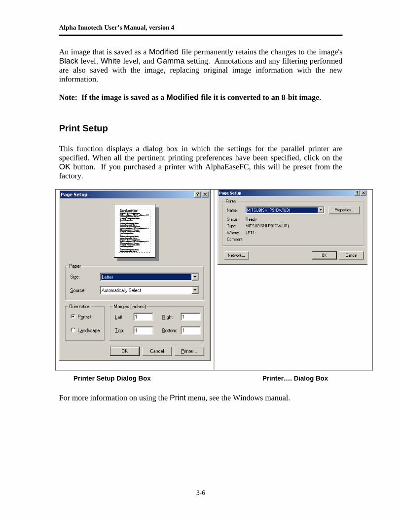
An image that is saved as a Modified file permanently retains the changes to the image's Black level, White level, and Gamma setting. Annotations and any filtering performed are also saved with the image, replacing original image information with the new information. Note: If the image is saved as a Modified file it is converted to an 8-bit image. Print Setup This function displays a dialog box in which the settings for the parallel printer are specified. When all the pertinent printing preferences have been specified, click on the OK button. If you purchased a printer with AlphaEaseFC, this will be preset from the factory.
Printer Setup Dialog Box Printer…. Dialog Box For more information on using the Print menu, see the Windows manual.
Chapter 3: Drop Down Menus
3-7
Print This function sends the image to the default printer specified in Print Setup. Logoff This function logs the current user out of AlphaEaseFC when security features are in use. For more information on security features, see Section 3.3. The Exit Function The Exit function closes AlphaEaseFC. To restart AlphaEaseFC from Windows, double-click on the AlphaEaseFC icon.
Alpha Innotech User’s Manual, version 4
3-8
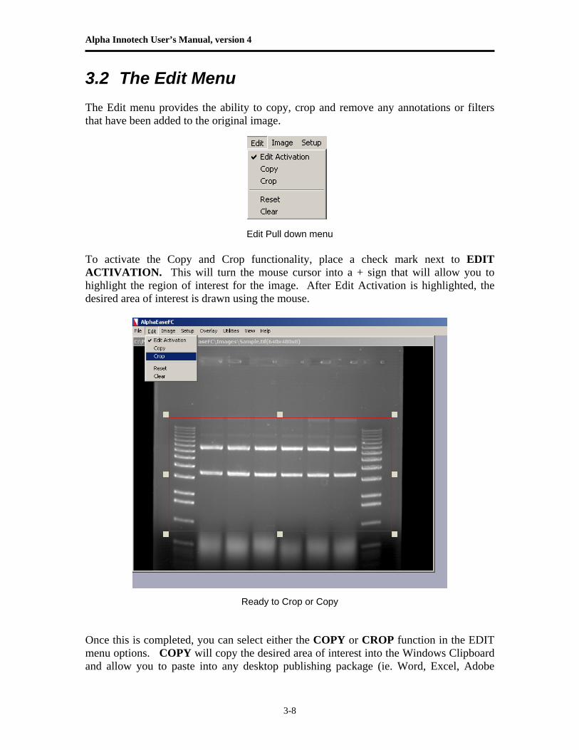
3.2 The Edit Menu The Edit menu provides the ability to copy, crop and remove any annotations or filters that have been added to the original image.
Edit Pull down menu To activate the Copy and Crop functionality, place a check mark next to EDIT ACTIVATION. This will turn the mouse cursor into a + sign that will allow you to highlight the region of interest for the image. After Edit Activation is highlighted, the desired area of interest is drawn using the mouse.
Ready to Crop or Copy
Once this is completed, you can select either the COPY or CROP function in the EDIT menu options. COPY will copy the desired area of interest into the Windows Clipboard and allow you to paste into any desktop publishing package (ie. Word, Excel, Adobe
Chapter 3: Drop Down Menus
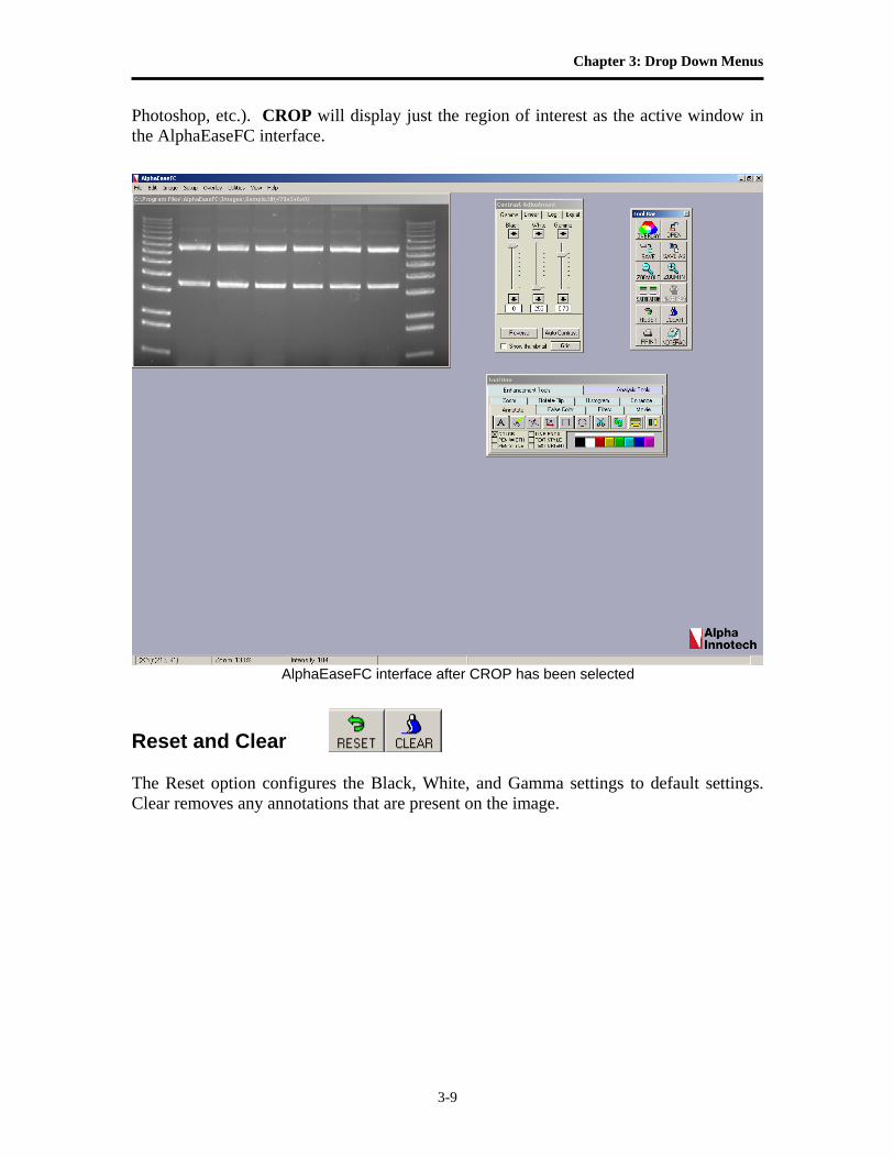
3-9
Photoshop, etc.). CROP will display just the region of interest as the active window in the AlphaEaseFC interface.
AlphaEaseFC interface after CROP has been selected
Reset and Clear The Reset option configures the Black, White, and Gamma settings to default settings. Clear removes any annotations that are present on the image.
Alpha Innotech User’s Manual, version 4
3-10
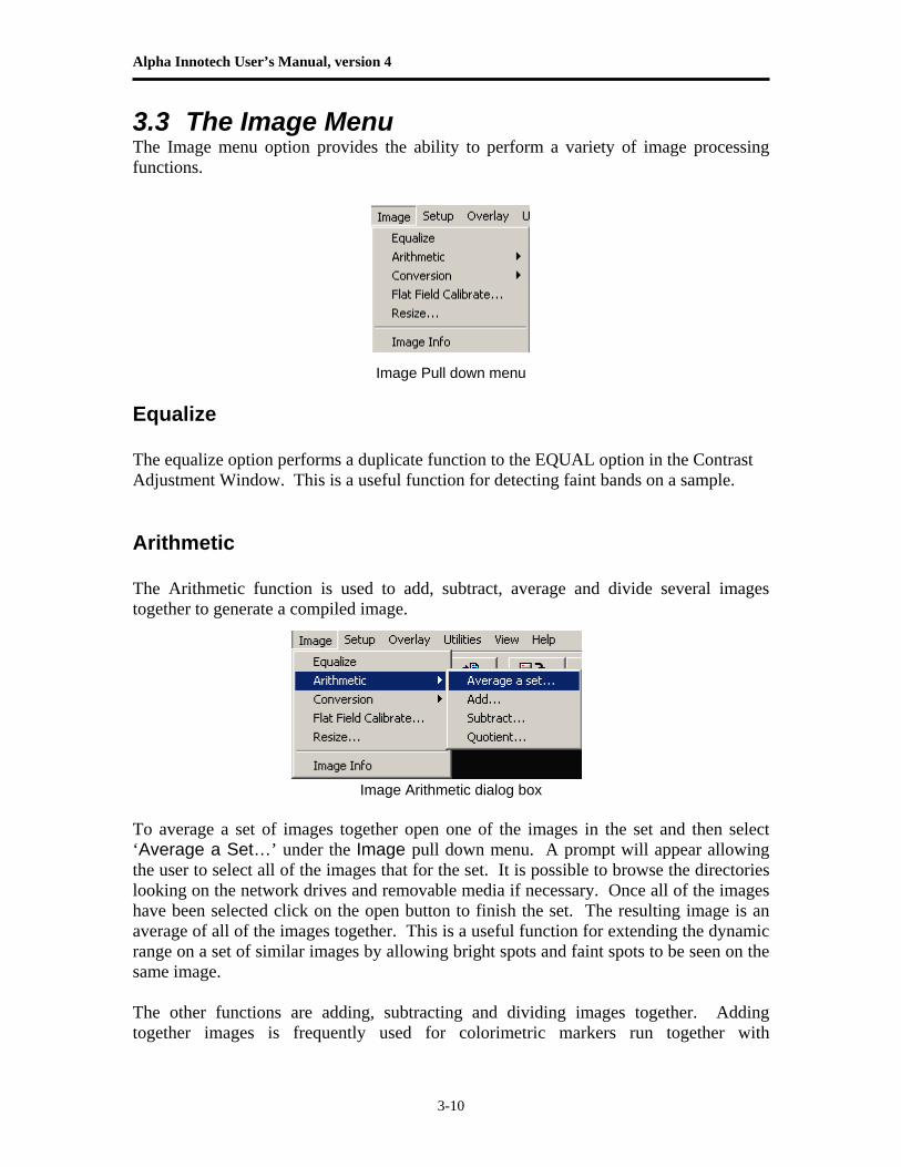
3.3 The Image Menu The Image menu option provides the ability to perform a variety of image processing functions.
Image Pull down menu Equalize The equalize option performs a duplicate function to the EQUAL option in the Contrast Adjustment Window. This is a useful function for detecting faint bands on a sample. Arithmetic The Arithmetic function is used to add, subtract, average and divide several images together to generate a compiled image.
Image Arithmetic dialog box To average a set of images together open one of the images in the set and then select ‘Average a Set…’ under the Image pull down menu. A prompt will appear allowing the user to select all of the images that for the set. It is possible to browse the directories looking on the network drives and removable media if necessary. Once all of the images have been selected click on the open button to finish the set. The resulting image is an average of all of the images together. This is a useful function for extending the dynamic range on a set of similar images by allowing bright spots and faint spots to be seen on the same image. The other functions are adding, subtracting and dividing images together. Adding together images is frequently used for colorimetric markers run together with
Chapter 3: Drop Down Menus
3-11
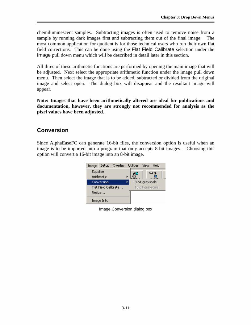
chemiluminescent samples. Subtracting images is often used to remove noise from a sample by running dark images first and subtracting them out of the final image. The most common application for quotient is for those technical users who run their own flat field corrections. This can be done using the Flat Field Calibrate selection under the Image pull down menu which will be described in detail later in this section. All three of these arithmetic functions are performed by opening the main image that will be adjusted. Next select the appropriate arithmetic function under the image pull down menu. Then select the image that is to be added, subtracted or divided from the original image and select open. The dialog box will disappear and the resultant image will appear. Note: Images that have been arithmetically altered are ideal for publications and documentation, however, they are strongly not recommended for analysis as the pixel values have been adjusted. Conversion Since AlphaEaseFC can generate 16-bit files, the conversion option is useful when an image is to be imported into a program that only accepts 8-bit images. Choosing this option will convert a 16-bit image into an 8-bit image.
Image Conversion dialog box
Alpha Innotech User’s Manual, version 4
3-12
Flat Field Calibrate Flat Field Calibrate is a function that is used to ‘flatten’ the image so that the pixel data is even across the entire image area. This is a function that is useful for large gels and other applications that use the entire field of view for an image. Creating flats can be art in itself; there are many documents on the internet that can help users interested in this arena to create the ideal flat for the application. However, some useful flats that have been created in the past involve very simple tools like a piece of 8.5 x 11 regular low quality copy paper (higher quality paper contains watermarks that will show up in the final image). It is essential that both the flat and the gel images be identical, including the aperture, zoom (if applicable) and focus settings on the lens. Step-by-Step Flat Field Calibration:
1) Place the gel or other application in the cabinet or dark room. 2) Adjust the aperture, zoom (if applicable) and focus on the lens. 3) Use auto-expose set to the normal selection and acquire an image of the gel.
(Alternatively, it is possible to select show saturation and then use expose preview and adjust the exposure time manually to just under saturation.)
4) Save the image of the gel. 5) Next remove the gel from the UV transilluminator or white light tray and clean
and/or dry off the surface if necessary using glass cleaner. 6) Place the white piece of paper onto the appropriate surface. (For example, if
the UV transilluminator was used, place the paper onto the UV transilluminator; if the white light tray was used, place the piece of paper onto the white light tray.)
7) Turn on the appropriate light source used (white light, UV transilluminator, epi lights, etc.).
8) Without changing anything on the lens acquire another image of the ‘Flat’ image following step #3 again.
9) Save the Flat image. 10) Open the original gel or other application image. 11) Select Flat Field Calibrate from the Image pull down menu. 12) Browse the directories for the ‘Flat’ image created. 13) Click on open. Make sure to save the flat field calibrated image for future use.
Chapter 3: Drop Down Menus
3-13
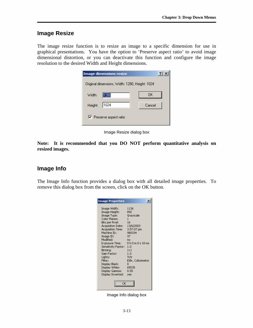
Image Resize The image resize function is to resize an image to a specific dimension for use in graphical presentations. You have the option to ‘Preserve aspect ratio’ to avoid image dimensional distortion, or you can deactivate this function and configure the image resolution to the desired Width and Height dimensions.
Image Resize dialog box
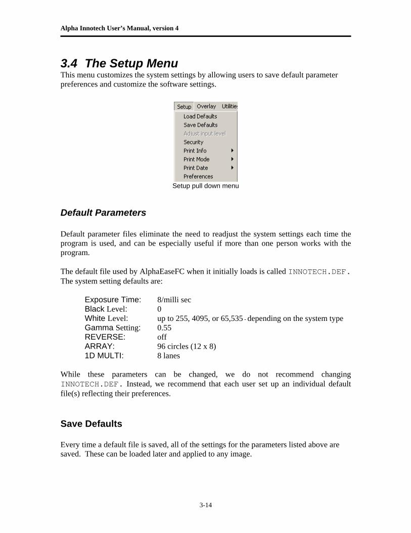
Note: It is recommended that you DO NOT perform quantitative analysis on resized images. Image Info The Image Info function provides a dialog box with all detailed image properties. To remove this dialog box from the screen, click on the OK button.
Image Info dialog box
Alpha Innotech User’s Manual, version 4
3-14
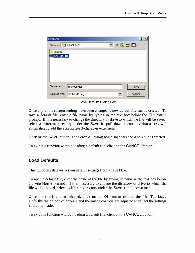
3.4 The Setup Menu This menu customizes the system settings by allowing users to save default parameter preferences and customize the software settings.
Setup pull down menu
Default Parameters Default parameter files eliminate the need to readjust the system settings each time the program is used, and can be especially useful if more than one person works with the program. The default file used by AlphaEaseFC when it initially loads is called INNOTECH.DEF. The system setting defaults are: Exposure Time: 8/milli sec Black Level: 0
White Level: up to 255, 4095, or 65,535 - depending on the system type Gamma Setting: 0.55 REVERSE: off ARRAY: 96 circles (12 x 8) 1D MULTI: 8 lanes While these parameters can be changed, we do not recommend changing INNOTECH.DEF. Instead, we recommend that each user set up an individual default file(s) reflecting their preferences. Save Defaults Every time a default file is saved, all of the settings for the parameters listed above are saved. These can be loaded later and applied to any image.
Chapter 3: Drop Down Menus
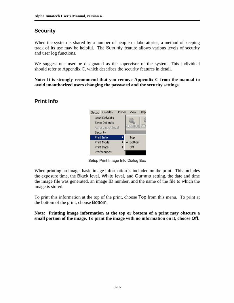
3-15
Save Defaults Dialog Box Once any of the system settings have been changed, a new default file can be created. To save a default file, enter a file name by typing in the text box below the File Name prompt. If it is necessary to change the directory or drive to which the file will be saved, select a different directory under the Save In pull down menu. AlphaEaseFC will automatically add the appropriate 3-character extension. Click on the SAVE button. The Save As dialog box disappears and a new file is created. To exit this function without loading a default file, click on the CANCEL button. Load Defaults This function retrieves system default settings from a saved file. To open a default file, enter the name of the file by typing its name in the text box below the File Name prompt. If it is necessary to change the directory or drive to which the file will be saved, select a different directory under the Save In pull down menu. Once the file has been selected, click on the OK button to load the file. The Load Defaults dialog box disappears and the image controls are adjusted to reflect the settings in the file loaded. To exit this function without loading a default file, click on the CANCEL button.
Alpha Innotech User’s Manual, version 4
3-16
Security When the system is shared by a number of people or laboratories, a method of keeping track of its use may be helpful. The Security feature allows various levels of security and user log functions. We suggest one user be designated as the supervisor of the system. This individual should refer to Appendix C, which describes the security features in detail. Note: It is strongly recommend that you remove Appendix C from the manual to avoid unauthorized users changing the password and the security settings. Print Info
Setup Print Image Info Dialog Box
When printing an image, basic image information is included on the print. This includes the exposure time, the Black level, White level, and Gamma setting, the date and time the image file was generated, an image ID number, and the name of the file to which the image is stored. To print this information at the top of the print, choose Top from this menu. To print at the bottom of the print, choose Bottom. Note: Printing image information at the top or bottom of a print may obscure a small portion of the image. To print the image with no information on it, choose Off.
Chapter 3: Drop Down Menus
3-17
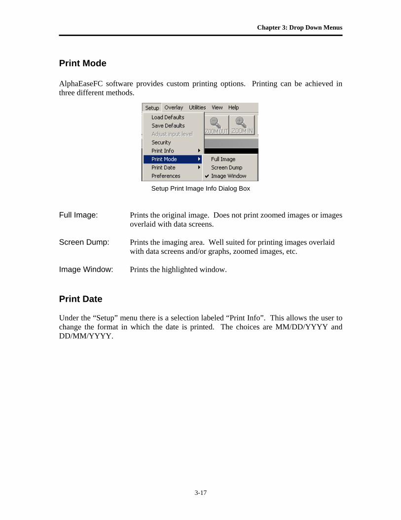
Print Mode AlphaEaseFC software provides custom printing options. Printing can be achieved in three different methods.
Setup Print Image Info Dialog Box Full Image: Prints the original image. Does not print zoomed images or images
overlaid with data screens. Screen Dump: Prints the imaging area. Well suited for printing images overlaid
with data screens and/or graphs, zoomed images, etc. Image Window: Prints the highlighted window. Print Date Under the “Setup” menu there is a selection labeled “Print Info”. This allows the user to change the format in which the date is printed. The choices are MM/DD/YYYY and DD/MM/YYYY.
Alpha Innotech User’s Manual, version 4
3-18
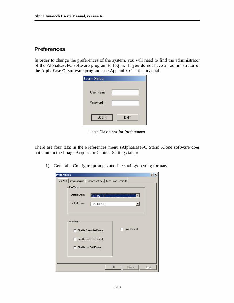
Preferences In order to change the preferences of the system, you will need to find the administrator of the AlphaEaseFC software program to log in. If you do not have an administrator of the AlphaEaseFC software program, see Appendix C in this manual.
Login Dialog box for Preferences There are four tabs in the Preferences menu (AlphaEaseFC Stand Alone software does not contain the Image Acquire or Cabinet Settings tabs):
1) General – Configure prompts and file saving/opening formats.
Chapter 3: Drop Down Menus
3-19
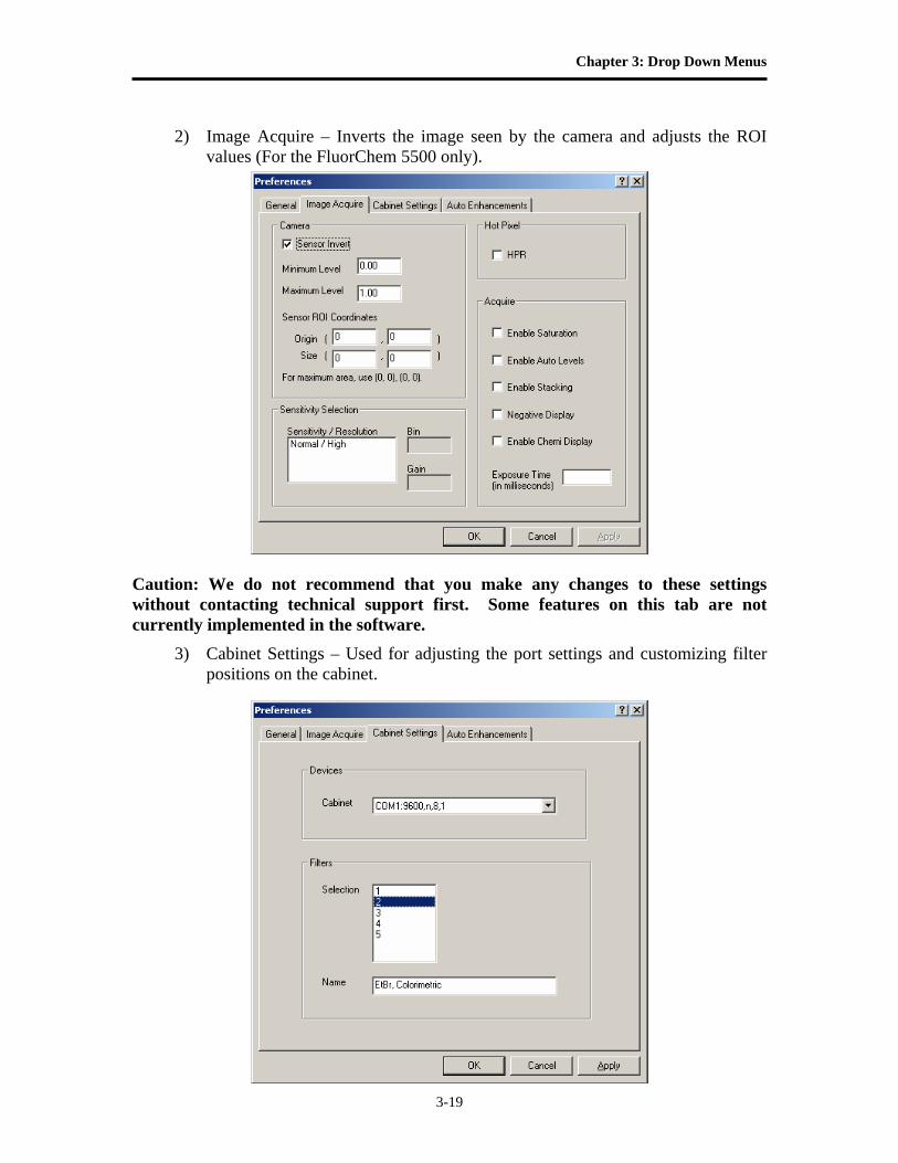
2) Image Acquire – Inverts the image seen by the camera and adjusts the ROI
values (For the FluorChem 5500 only).
Caution: We do not recommend that you make any changes to these settings without contacting technical support first. Some features on this tab are not currently implemented in the software.
3) Cabinet Settings – Used for adjusting the port settings and customizing filter positions on the cabinet.
Alpha Innotech User’s Manual, version 4
3-20
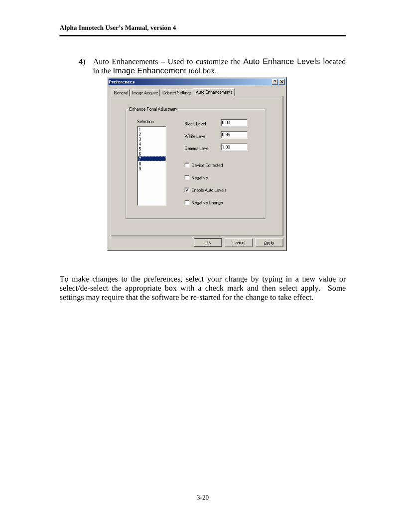
4) Auto Enhancements – Used to customize the Auto Enhance Levels located
in the Image Enhancement tool box. To make changes to the preferences, select your change by typing in a new value or select/de-select the appropriate box with a check mark and then select apply. Some settings may require that the software be re-started for the change to take effect.
Chapter 3: Drop Down Menus
3-21
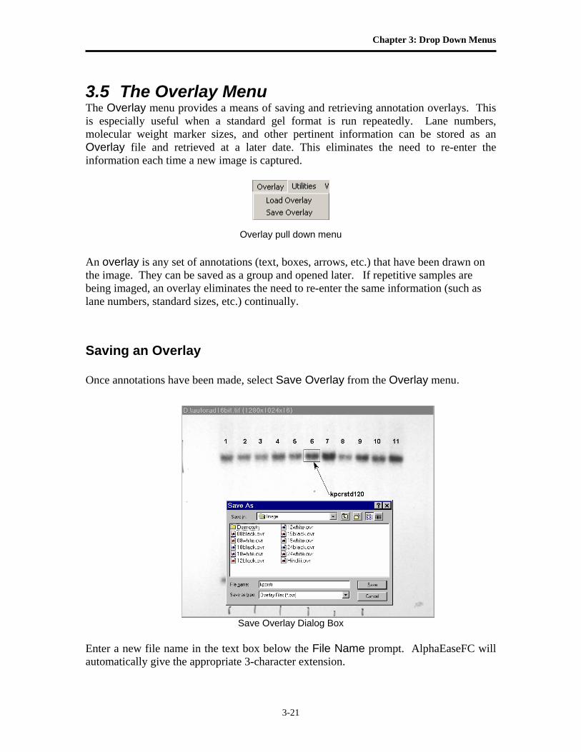
3.5 The Overlay Menu The Overlay menu provides a means of saving and retrieving annotation overlays. This is especially useful when a standard gel format is run repeatedly. Lane numbers, molecular weight marker sizes, and other pertinent information can be stored as an Overlay file and retrieved at a later date. This eliminates the need to re-enter the information each time a new image is captured.
Overlay pull down menu
An overlay is any set of annotations (text, boxes, arrows, etc.) that have been drawn on the image. They can be saved as a group and opened later. If repetitive samples are being imaged, an overlay eliminates the need to re-enter the same information (such as lane numbers, standard sizes, etc.) continually. Saving an Overlay Once annotations have been made, select Save Overlay from the Overlay menu.
Save Overlay Dialog Box Enter a new file name in the text box below the File Name prompt. AlphaEaseFC will automatically give the appropriate 3-character extension.
Alpha Innotech User’s Manual, version 4
3-22
The current directory is the one in which the new overlay file will be saved. If necessary, change the directory or drive as described in Section 3.1. Once a name has been entered and the appropriate directory has been accessed, click the SAVE button to save the overlay file. Loading an Overlay The Load Overlay function allows Overlay files to be retrieved and applied to the image currently displayed. Opening an Overlay after an image has been captured places the annotations on top of the image. They can be stored as part of the image by saving the file as a modified file. (See Save Image As in Section 3.1 for instructions.)
Select the name of the file to be loaded. (If necessary, change the directory or drive.) The file name is then highlighted in the list and appears in the text box below the Filename prompt. Once the file has been selected, click on the OK button to load the file. (Alternatively, double-click on the file name.) The dialog box disappears and the annotations in the selected file appear on the image. To dismiss the dialog box without loading annotations, click on the CANCEL button. Overlay Libraries AlphaEaseFC contains a library of overlays that can be accessed through the Load Overlay function described above. This library of overlays is stored in the Image folder located in the AlphaEaseFC directory:
08WHITE.OVR / 08BLACK.OVR 8 lane labels in white/black 10WHITE.OVR / 10BLACK.OVR 10 lane labels in white/black 12WHITE.OVR / 12BLACK.OVR 12 lane labels in white/black 15WHITE.OVR / 15BLACK.OVR 15 lane labels in white/black 24WHITE.OVR / 24BLACK.OVR 24 lane labels in white/black HINDIII.OVR λHindIII label
The objects in these overlays can be repositioned, resized, re-colored, copied or deleted as needed.
Chapter 3: Drop Down Menus
3-23
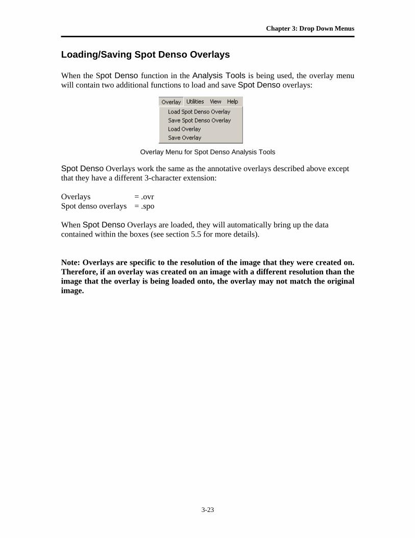
Loading/Saving Spot Denso Overlays When the Spot Denso function in the Analysis Tools is being used, the overlay menu will contain two additional functions to load and save Spot Denso overlays:
Overlay Menu for Spot Denso Analysis Tools
Spot Denso Overlays work the same as the annotative overlays described above except that they have a different 3-character extension: Overlays = .ovr Spot denso overlays = .spo When Spot Denso Overlays are loaded, they will automatically bring up the data contained within the boxes (see section 5.5 for more details). Note: Overlays are specific to the resolution of the image that they were created on. Therefore, if an overlay was created on an image with a different resolution than the image that the overlay is being loaded onto, the overlay may not match the original image.
Alpha Innotech User’s Manual, version 4
3-24
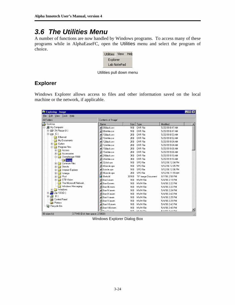
3.6 The Utilities Menu A number of functions are now handled by Windows programs. To access many of these programs while in AlphaEaseFC, open the Utilities menu and select the program of choice.
Utilities pull down menu Explorer Windows Explorer allows access to files and other information saved on the local machine or the network, if applicable.
Windows Explorer Dialog Box
Chapter 3: Drop Down Menus
3-25
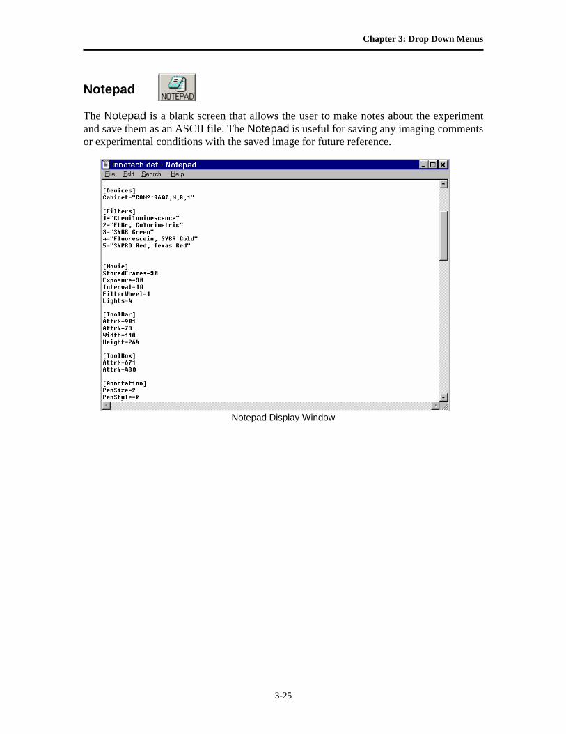
Notepad The Notepad is a blank screen that allows the user to make notes about the experiment and save them as an ASCII file. The Notepad is useful for saving any imaging comments or experimental conditions with the saved image for future reference.
Notepad Display Window
Alpha Innotech User’s Manual, version 4
3-26
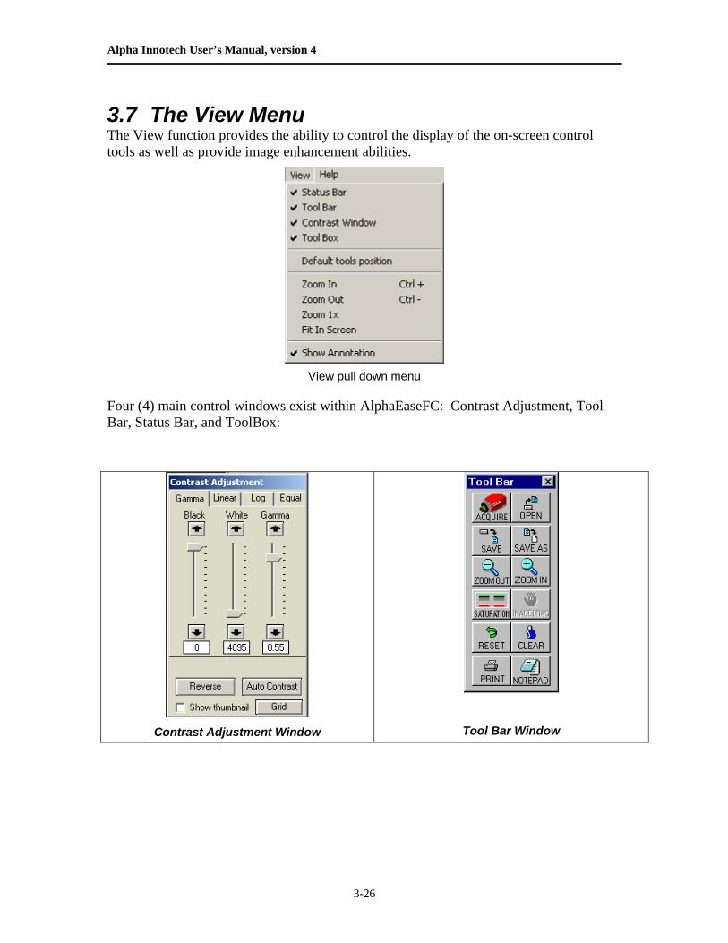
3.7 The View Menu The View function provides the ability to control the display of the on-screen control tools as well as provide image enhancement abilities.
View pull down menu
Four (4) main control windows exist within AlphaEaseFC: Contrast Adjustment, Tool Bar, Status Bar, and ToolBox:
Contrast Adjustment Window
Tool Bar Window
Chapter 3: Drop Down Menus
3-27
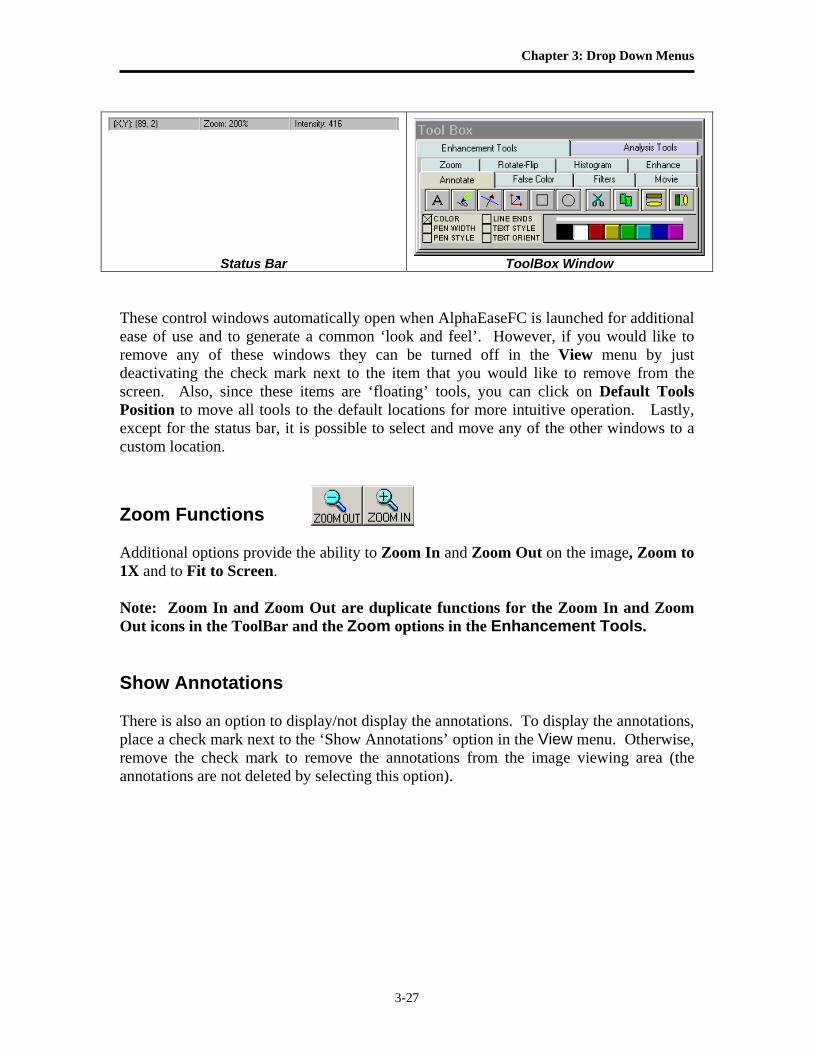
These control windows automatically open when AlphaEaseFC is launched for additional ease of use and to generate a common ‘look and feel’. However, if you would like to remove any of these windows they can be turned off in the View menu by just deactivating the check mark next to the item that you would like to remove from the screen. Also, since these items are ‘floating’ tools, you can click on Default Tools Position to move all tools to the default locations for more intuitive operation. Lastly, except for the status bar, it is possible to select and move any of the other windows to a custom location.
Zoom Functions Additional options provide the ability to Zoom In and Zoom Out on the image, Zoom to 1X and to Fit to Screen. Note: Zoom In and Zoom Out are duplicate functions for the Zoom In and Zoom Out icons in the ToolBar and the Zoom options in the Enhancement Tools. Show Annotations There is also an option to display/not display the annotations. To display the annotations, place a check mark next to the ‘Show Annotations’ option in the View menu. Otherwise, remove the check mark to remove the annotations from the image viewing area (the annotations are not deleted by selecting this option).
Status Bar ToolBox Window
Alpha Innotech User’s Manual, version 4
3-28
3.8 The Help Menu
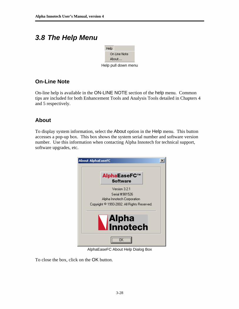
Help pull down menu On-Line Note On-line help is available in the ON-LINE NOTE section of the help menu. Common tips are included for both Enhancement Tools and Analysis Tools detailed in Chapters 4 and 5 respectively. About To display system information, select the About option in the Help menu. This button accesses a pop-up box. This box shows the system serial number and software version number. Use this information when contacting Alpha Innotech for technical support, software upgrades, etc.
AlphaEaseFC About Help Dialog Box To close the box, click on the OK button.

Chapter 3: Drop Down Menus
3-29
BLANK PAGE

Alpha Innotech User’s Manual, version 4
3-30
BLANK PAGE
Chapter 4: Enhancement Tools
4-1
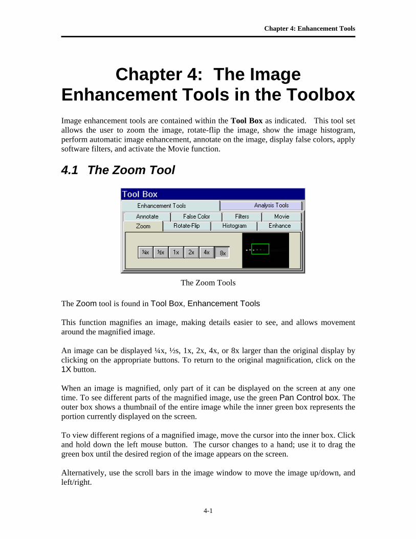
Chapter 4: The Image Enhancement Tools in the Toolbox Image enhancement tools are contained within the Tool Box as indicated. This tool set allows the user to zoom the image, rotate-flip the image, show the image histogram, perform automatic image enhancement, annotate on the image, display false colors, apply software filters, and activate the Movie function. 4.1 The Zoom Tool
The Zoom Tools The Zoom tool is found in Tool Box, Enhancement Tools This function magnifies an image, making details easier to see, and allows movement around the magnified image. An image can be displayed ¼x, ½s, 1x, 2x, 4x, or 8x larger than the original display by clicking on the appropriate buttons. To return to the original magnification, click on the 1X button. When an image is magnified, only part of it can be displayed on the screen at any one time. To see different parts of the magnified image, use the green Pan Control box. The outer box shows a thumbnail of the entire image while the inner green box represents the portion currently displayed on the screen. To view different regions of a magnified image, move the cursor into the inner box. Click and hold down the left mouse button. The cursor changes to a hand; use it to drag the green box until the desired region of the image appears on the screen. Alternatively, use the scroll bars in the image window to move the image up/down, and left/right.
Alpha Innotech User’s Manual, version 4
4-2
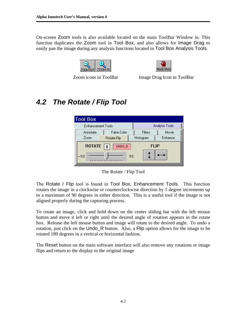
On-screen Zoom tools is also available located on the main ToolBar Window in. This function duplicates the Zoom tool in Tool Box, and also allows for Image Drag to easily pan the image during any analysis functions located in Tool Box Analysis Tools.
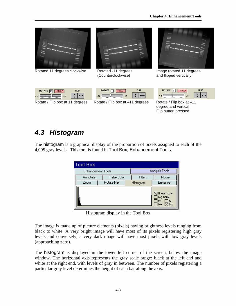
Zoom icons in ToolBar Image Drag Icon in ToolBar 4.2 The Rotate / Flip Tool
The Rotate / Flip Tool The Rotate / Flip tool is found in Tool Box, Enhancement Tools. This function rotates the image in a clockwise or counterclockwise direction by 1 degree increments up to a maximum of 90 degrees in either direction. This is a useful tool if the image is not aligned properly during the capturing process. To rotate an image, click and hold down on the center sliding bar with the left mouse button and move it left or right until the desired angle of rotation appears in the rotate box. Release the left mouse button and image will rotate to the desired angle. To undo a rotation, just click on the Undo_R button. Also, a Flip option allows for the image to be rotated 180 degrees in a vertical or horizontal fashion. The Reset button on the main software interface will also remove any rotations or image flips and return to the display to the original image
Chapter 4: Enhancement Tools
4-3
Rotated 11 degrees clockwise Rotated -11 degrees Image rotated 11 degrees (Counterclockwise) and flipped vertically
Rotate / Flip box at 11 degrees Rotate / Flip box at –11 degrees Rotate / Flip box at –11 degree and vertical Flip button pressed
4.3 Histogram The histogram is a graphical display of the proportion of pixels assigned to each of the 4,095 gray levels. This tool is found in Tool Box, Enhancement Tools.
Histogram display in the Tool Box
The image is made up of picture elements (pixels) having brightness levels ranging from black to white. A very bright image will have most of its pixels registering high gray levels and conversely, a very dark image will have most pixels with low gray levels (approaching zero). The histogram is displayed in the lower left corner of the screen, below the image window. The horizontal axis represents the gray scale range: black at the left end and white at the right end, with levels of gray in between. The number of pixels registering a particular gray level determines the height of each bar along the axis.
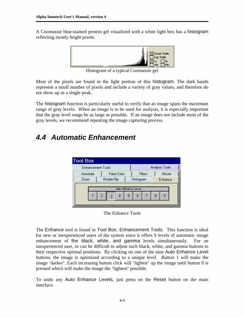
Alpha Innotech User’s Manual, version 4
4-4
A Coomassie blue-stained protein gel visualized with a white light box has a histogram reflecting mostly bright pixels:
Histogram of a typical Coomassie gel
Most of the pixels are found in the light portion of this histogram. The dark bands represent a small number of pixels and include a variety of gray values, and therefore do not show up as a single peak. The histogram function is particularly useful to verify that an image spans the maximum range of gray levels. When an image is to be used for analysis, it is especially important that the gray level range be as large as possible. If an image does not include most of the gray levels, we recommend repeating the image capturing process.
4.4 Automatic Enhancement
The Enhance Tools The Enhance tool is found in Tool Box, Enhancement Tools. This function is ideal for new or inexperienced users of the system since it offers 9 levels of automatic image enhancement of the black, white, and gamma levels simultaneously. For an inexperienced user, in can be difficult to adjust each black, white, and gamma buttons to their respective optimal positions. By clicking on one of the nine Auto Enhance Level buttons, the image is optimized according to a unique level. Button 1 will make the image ‘darker’. Each increasing button click will ‘lighten’ up the image until button 9 is pressed which will make the image the ‘lightest’ possible. To undo any Auto Enhance Levels, just press on the Reset button on the main interface.
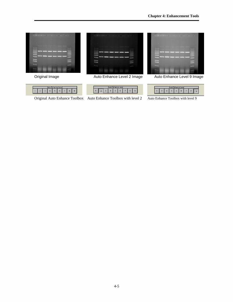
Chapter 4: Enhancement Tools
4-5
Original Image Auto Enhance Level 2 Image Auto Enhance Level 9 Image
Original Auto Enhance Toolbox Auto Enhance Toolbox with level 2 Auto Enhance Toolbox with level 9
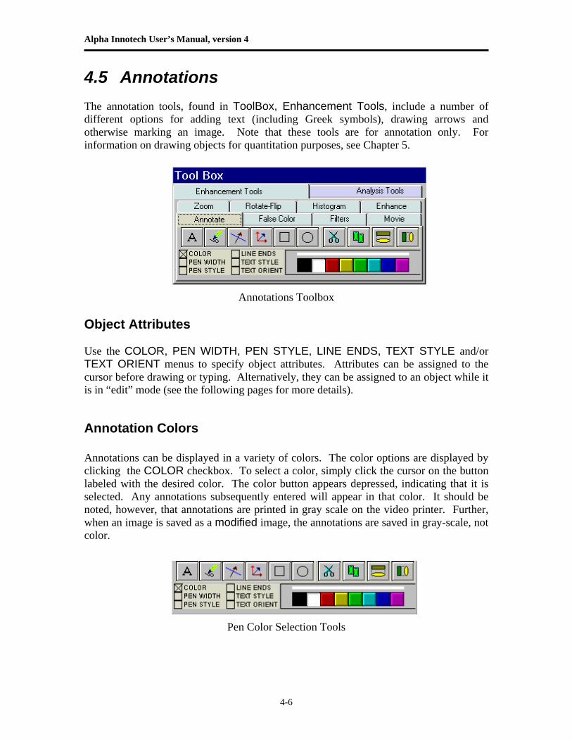
Alpha Innotech User’s Manual, version 4
4-6
4.5 Annotations The annotation tools, found in ToolBox, Enhancement Tools, include a number of different options for adding text (including Greek symbols), drawing arrows and otherwise marking an image. Note that these tools are for annotation only. For information on drawing objects for quantitation purposes, see Chapter 5.
Annotations Toolbox Object Attributes Use the COLOR, PEN WIDTH, PEN STYLE, LINE ENDS, TEXT STYLE and/or TEXT ORIENT menus to specify object attributes. Attributes can be assigned to the cursor before drawing or typing. Alternatively, they can be assigned to an object while it is in “edit” mode (see the following pages for more details).
Annotation Colors Annotations can be displayed in a variety of colors. The color options are displayed by clicking the COLOR checkbox. To select a color, simply click the cursor on the button labeled with the desired color. The color button appears depressed, indicating that it is selected. Any annotations subsequently entered will appear in that color. It should be noted, however, that annotations are printed in gray scale on the video printer. Further, when an image is saved as a modified image, the annotations are saved in gray-scale, not color.
Pen Color Selection Tools
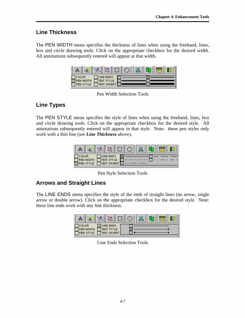
Chapter 4: Enhancement Tools
4-7
Line Thickness The PEN WIDTH menu specifies the thickness of lines when using the freehand, lines, box and circle drawing tools. Click on the appropriate checkbox for the desired width. All annotations subsequently entered will appear at that width.
Pen Width Selection Tools
Line Types The PEN STYLE menu specifies the style of lines when using the freehand, lines, box and circle drawing tools. Click on the appropriate checkbox for the desired style. All annotations subsequently entered will appear in that style. Note: these pen styles only work with a thin line (see Line Thickness above).
Pen Style Selection Tools
Arrows and Straight Lines The LINE ENDS menu specifies the style of the ends of straight lines (no arrow, single arrow or double arrow). Click on the appropriate checkbox for the desired style. Note: these line ends work with any line thickness.
Line Ends Selection Tools
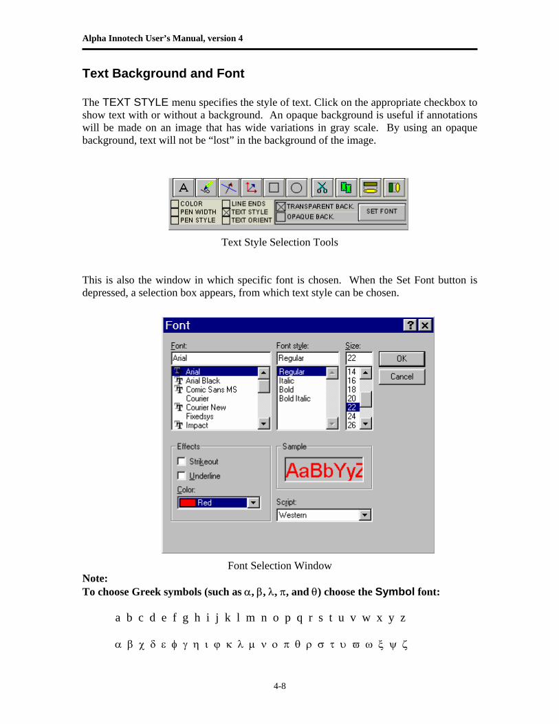
Alpha Innotech User’s Manual, version 4
4-8
Text Background and Font The TEXT STYLE menu specifies the style of text. Click on the appropriate checkbox to show text with or without a background. An opaque background is useful if annotations will be made on an image that has wide variations in gray scale. By using an opaque background, text will not be “lost” in the background of the image.
Text Style Selection Tools This is also the window in which specific font is chosen. When the Set Font button is depressed, a selection box appears, from which text style can be chosen.
Font Selection Window Note: To choose Greek symbols (such as α, β, λ, π, and θ) choose the Symbol font: a b c d e f g h i j k l m n o p q r s t u v w x y z α β χ δ ε φ γ η ι ϕ κ λ µ ν ο π θ ρ σ τ υ ϖ ω ξ ψ ζ
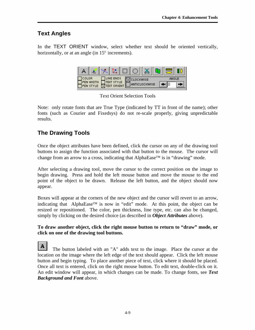
Chapter 4: Enhancement Tools
4-9
Text Angles In the TEXT ORIENT window, select whether text should be oriented vertically, horizontally, or at an angle (in 15° increments).
Text Orient Selection Tools Note: only rotate fonts that are True Type (indicated by TT in front of the name); other fonts (such as Courier and Fixedsys) do not re-scale properly, giving unpredictable results. The Drawing Tools Once the object attributes have been defined, click the cursor on any of the drawing tool buttons to assign the function associated with that button to the mouse. The cursor will change from an arrow to a cross, indicating that AlphaEase™ is in “drawing” mode. After selecting a drawing tool, move the cursor to the correct position on the image to begin drawing. Press and hold the left mouse button and move the mouse to the end point of the object to be drawn. Release the left button, and the object should now appear. Boxes will appear at the corners of the new object and the cursor will revert to an arrow, indicating that AlphaEase™ is now in “edit” mode. At this point, the object can be resized or repositioned. The color, pen thickness, line type, etc. can also be changed, simply by clicking on the desired choice (as described in Object Attributes above). To draw another object, click the right mouse button to return to “draw” mode, or click on one of the drawing tool buttons.
The button labeled with an "A" adds text to the image. Place the cursor at the location on the image where the left edge of the text should appear. Click the left mouse button and begin typing. To place another piece of text, click where it should be placed. Once all text is entered, click on the right mouse button. To edit text, double-click on it. An edit window will appear, in which changes can be made. To change fonts, see Text Background and Font above.
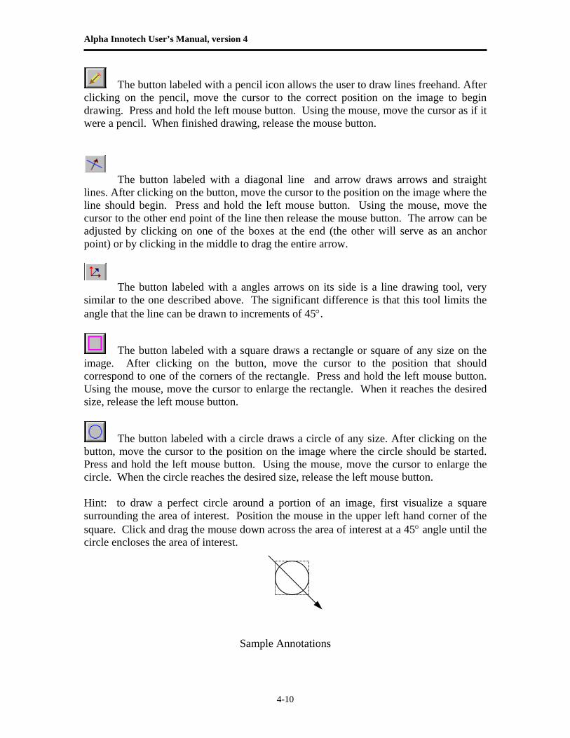
Alpha Innotech User’s Manual, version 4
4-10
The button labeled with a pencil icon allows the user to draw lines freehand. After clicking on the pencil, move the cursor to the correct position on the image to begin drawing. Press and hold the left mouse button. Using the mouse, move the cursor as if it were a pencil. When finished drawing, release the mouse button.
The button labeled with a diagonal line and arrow draws arrows and straight lines. After clicking on the button, move the cursor to the position on the image where the line should begin. Press and hold the left mouse button. Using the mouse, move the cursor to the other end point of the line then release the mouse button. The arrow can be adjusted by clicking on one of the boxes at the end (the other will serve as an anchor point) or by clicking in the middle to drag the entire arrow.
The button labeled with a angles arrows on its side is a line drawing tool, very similar to the one described above. The significant difference is that this tool limits the angle that the line can be drawn to increments of 45°.
The button labeled with a square draws a rectangle or square of any size on the image. After clicking on the button, move the cursor to the position that should correspond to one of the corners of the rectangle. Press and hold the left mouse button. Using the mouse, move the cursor to enlarge the rectangle. When it reaches the desired size, release the left mouse button.
The button labeled with a circle draws a circle of any size. After clicking on the button, move the cursor to the position on the image where the circle should be started. Press and hold the left mouse button. Using the mouse, move the cursor to enlarge the circle. When the circle reaches the desired size, release the left mouse button. Hint: to draw a perfect circle around a portion of an image, first visualize a square surrounding the area of interest. Position the mouse in the upper left hand corner of the square. Click and drag the mouse down across the area of interest at a 45° angle until the circle encloses the area of interest.
Sample Annotations
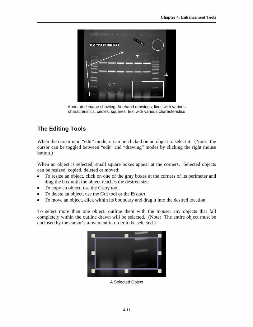
Chapter 4: Enhancement Tools
4-11
Annotated image showing: freehand drawings, lines with various characteristics, circles, squares, text with various characteristics
The Editing Tools When the cursor is in “edit” mode, it can be clicked on an object to select it. (Note: the cursor can be toggled between “edit” and “drawing” modes by clicking the right mouse button.) When an object is selected, small square boxes appear at the corners. Selected objects can be resized, copied, deleted or moved: • To resize an object, click on one of the gray boxes at the corners of its perimeter and
drag the box until the object reaches the desired size. • To copy an object, use the Copy tool. • To delete an object, use the Cut tool or the Eraser. • To move an object, click within its boundary and drag it into the desired location. To select more than one object, outline them with the mouse; any objects that fall completely within the outline drawn will be selected. (Note: The entire object must be enclosed by the cursor’s movement in order to be selected.)
A Selected Object
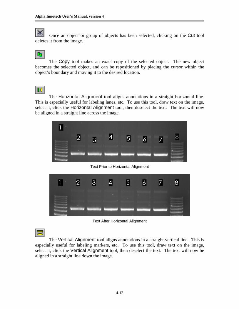
Alpha Innotech User’s Manual, version 4
4-12
Once an object or group of objects has been selected, clicking on the Cut tool deletes it from the image.
The Copy tool makes an exact copy of the selected object. The new object becomes the selected object, and can be repositioned by placing the cursor within the object’s boundary and moving it to the desired location.
The Horizontal Alignment tool aligns annotations in a straight horizontal line. This is especially useful for labeling lanes, etc. To use this tool, draw text on the image, select it, click the Horizontal Alignment tool, then deselect the text. The text will now be aligned in a straight line across the image.
Text Prior to Horizontal Alignment
Text After Horizontal Alignment
The Vertical Alignment tool aligns annotations in a straight vertical line. This is especially useful for labeling markers, etc. To use this tool, draw text on the image, select it, click the Vertical Alignment tool, then deselect the text. The text will now be aligned in a straight line down the image.
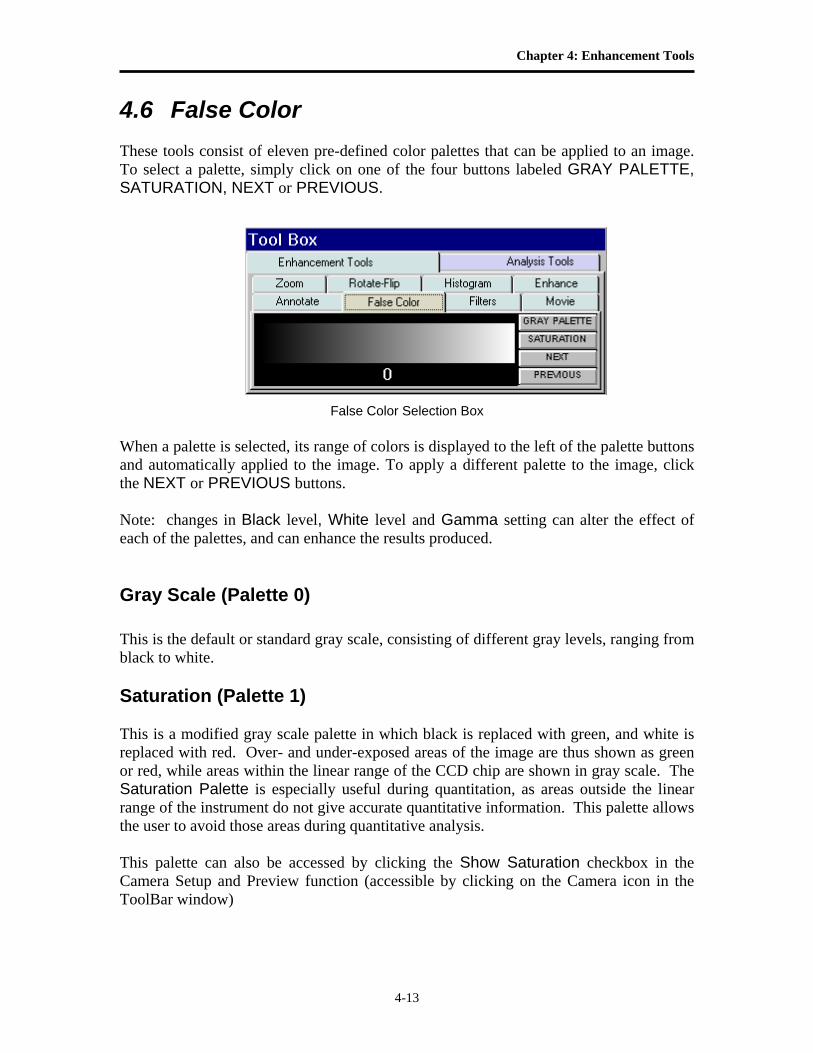
Chapter 4: Enhancement Tools
4-13
4.6 False Color
These tools consist of eleven pre-defined color palettes that can be applied to an image. To select a palette, simply click on one of the four buttons labeled GRAY PALETTE, SATURATION, NEXT or PREVIOUS.
False Color Selection Box When a palette is selected, its range of colors is displayed to the left of the palette buttons and automatically applied to the image. To apply a different palette to the image, click the NEXT or PREVIOUS buttons. Note: changes in Black level, White level and Gamma setting can alter the effect of each of the palettes, and can enhance the results produced. Gray Scale (Palette 0) This is the default or standard gray scale, consisting of different gray levels, ranging from black to white. Saturation (Palette 1) This is a modified gray scale palette in which black is replaced with green, and white is replaced with red. Over- and under-exposed areas of the image are thus shown as green or red, while areas within the linear range of the CCD chip are shown in gray scale. The Saturation Palette is especially useful during quantitation, as areas outside the linear range of the instrument do not give accurate quantitative information. This palette allows the user to avoid those areas during quantitative analysis. This palette can also be accessed by clicking the Show Saturation checkbox in the Camera Setup and Preview function (accessible by clicking on the Camera icon in the ToolBar window)
Alpha Innotech User’s Manual, version 4
4-14
Palettes 2 through 11 These are color substitution palettes in which the gray levels are translated into different color ranges. These palettes can be useful to help distinguish features and highlight details on an image. Palette 2 maps the gray scale levels to a red/green/blue palette. Values of 0 are mapped to red; saturated to blue, and values in between to green. Palette 3 maps the gray scale levels to a red/green/blue palette. Values of 0 are mapped to blue; saturated to green, and values in between to red. Palette 4 maps the gray scale levels to a red/green/blue palette. Values of 0 are mapped to green; saturated to red, and values in between to blue. Palette 5 maps the gray scale levels to a cyan/magenta/yellow palette. Values of 0 are mapped to cyan; saturated to yellow, and values in between to magenta. Palette 6 maps the gray scale levels to a cyan/magenta/yellow palette. Values of 0 are mapped to yellow; saturated to magenta, and values in between to cyan. Palette 7 maps the gray scale levels to a cyan/magenta/yellow palette. Values of 0 are mapped to magenta; saturated to cyan, and values in between to yellow. Palette 8 maps the gray scale levels to a red palette. Values of 0 are mapped to dark red; saturated to white, and values in between to shades of red. Palette 9 maps the gray scale levels to a blue palette. Values of 0 are mapped to dark blue; saturated to white, and values in between to shades of blue. This palette may be useful when printing an image of a Coomassie-stained protein gel onto a color printer. Palette 10 maps the gray scale levels to a green palette. Values of 0 are mapped to dark green; saturated to white, and values in between to shades of green. This palette may be useful when printing an image of a SYBR® Green I-stained protein gel onto a color printer. Palette 11 maps the gray scale levels to an orange palette. Values of 0 are mapped to dark orange; saturated to white, and values in between to shades of orange. This palette may be useful when printing an image of an EtBr-stained gel onto a color printer.
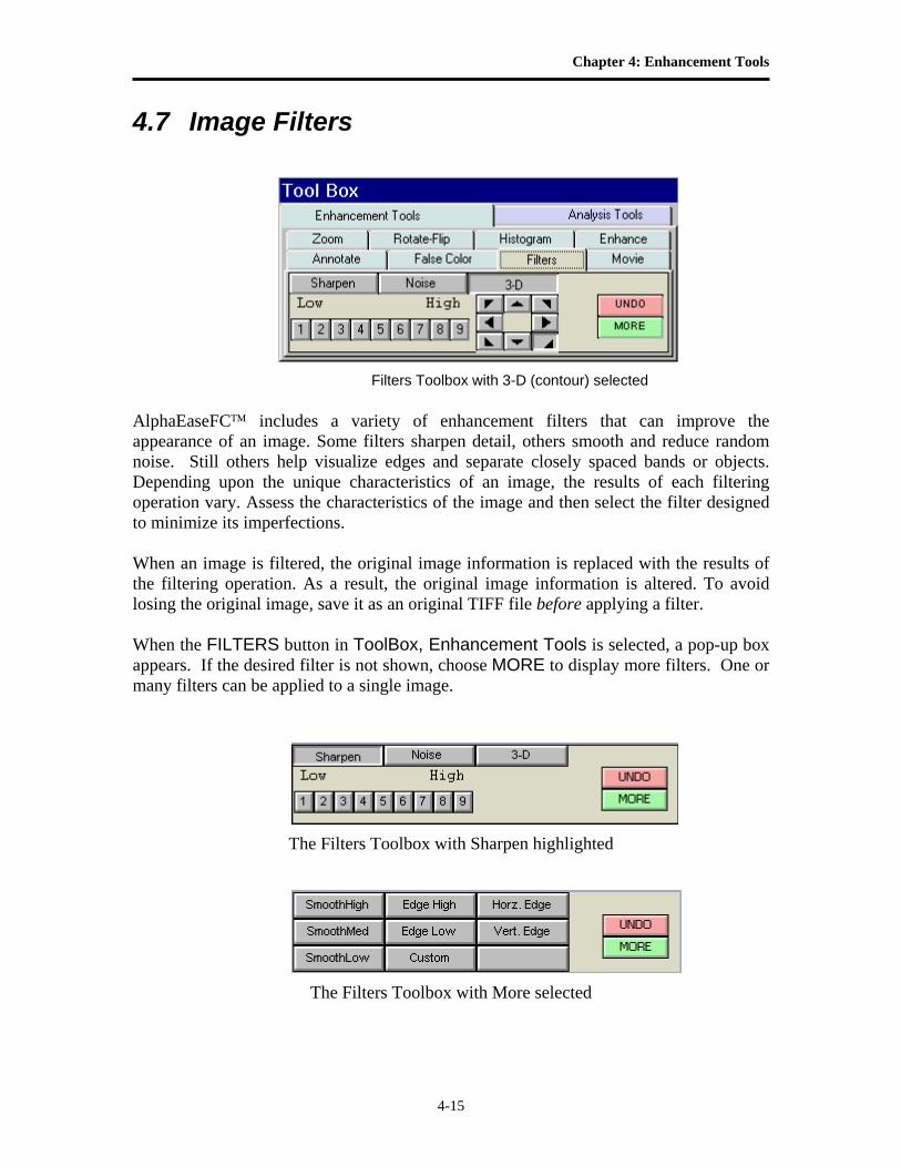
Chapter 4: Enhancement Tools
4-15
4.7 Image Filters
Filters Toolbox with 3-D (contour) selected AlphaEaseFC™ includes a variety of enhancement filters that can improve the appearance of an image. Some filters sharpen detail, others smooth and reduce random noise. Still others help visualize edges and separate closely spaced bands or objects. Depending upon the unique characteristics of an image, the results of each filtering operation vary. Assess the characteristics of the image and then select the filter designed to minimize its imperfections. When an image is filtered, the original image information is replaced with the results of the filtering operation. As a result, the original image information is altered. To avoid losing the original image, save it as an original TIFF file before applying a filter. When the FILTERS button in ToolBox, Enhancement Tools is selected, a pop-up box appears. If the desired filter is not shown, choose MORE to display more filters. One or many filters can be applied to a single image.
The Filters Toolbox with Sharpen highlighted
The Filters Toolbox with More selected
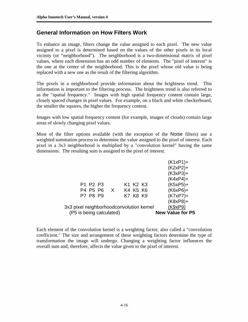
Alpha Innotech User’s Manual, version 4
4-16
General Information on How Filters Work To enhance an image, filters change the value assigned to each pixel. The new value assigned to a pixel is determined based on the values of the other pixels in its local vicinity (or “neighborhood”). The neighborhood is a two-dimensional matrix of pixel values, where each dimension has an odd number of elements. The "pixel of interest" is the one at the center of the neighborhood. This is the pixel whose old value is being replaced with a new one as the result of the filtering algorithm. The pixels in a neighborhood provide information about the brightness trend. This information is important to the filtering process. The brightness trend is also referred to as the "spatial frequency." Images with high spatial frequency content contain large, closely spaced changes in pixel values. For example, on a black and white checkerboard, the smaller the squares, the higher the frequency content. Images with low spatial frequency content (for example, images of clouds) contain large areas of slowly changing pixel values. Most of the filter options available (with the exception of the Noise filters) use a weighted summation process to determine the value assigned to the pixel of interest. Each pixel in a 3x3 neighborhood is multiplied by a "convolution kernel" having the same dimensions. The resulting sum is assigned to the pixel of interest.
(K1xP1)+ (K2xP2)+ (K3xP3)+ (K4xP4)+ P1 P2 P3 K1 K2 K3 (K5xP5)+ P4 P5 P6 X K4 K5 K6 (K6xP6)+ P7 P8 P9 K7 K8 K9 (K7xP7)+ (K8xP8)+
3x3 pixel neighborhoodconvolution kernel (K9xP9) (P5 is being calculated) New Value for P5
Each element of the convolution kernel is a weighting factor, also called a "convolution coefficient." The size and arrangement of these weighting factors determine the type of transformation the image will undergo. Changing a weighting factor influences the overall sum and, therefore, affects the value given to the pixel of interest.
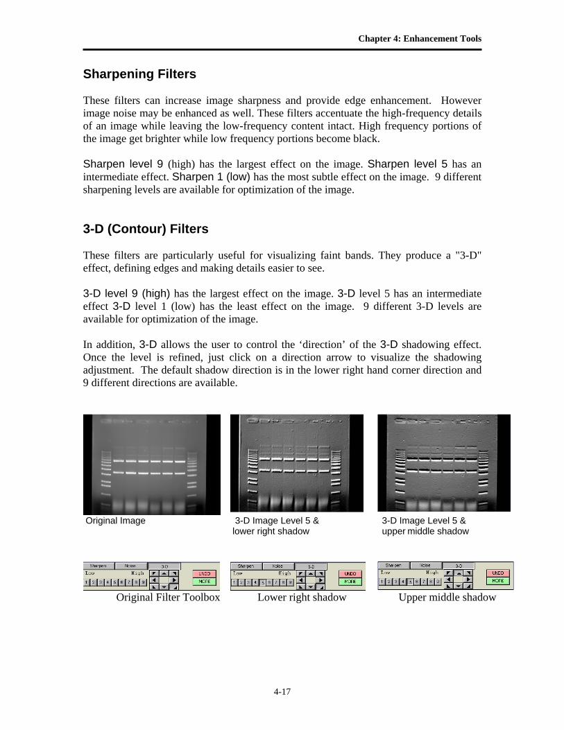
Chapter 4: Enhancement Tools
4-17
Sharpening Filters These filters can increase image sharpness and provide edge enhancement. However image noise may be enhanced as well. These filters accentuate the high-frequency details of an image while leaving the low-frequency content intact. High frequency portions of the image get brighter while low frequency portions become black. Sharpen level 9 (high) has the largest effect on the image. Sharpen level 5 has an intermediate effect. Sharpen 1 (low) has the most subtle effect on the image. 9 different sharpening levels are available for optimization of the image. 3-D (Contour) Filters These filters are particularly useful for visualizing faint bands. They produce a "3-D" effect, defining edges and making details easier to see. 3-D level 9 (high) has the largest effect on the image. 3-D level 5 has an intermediate effect 3-D level 1 (low) has the least effect on the image. 9 different 3-D levels are available for optimization of the image. In addition, 3-D allows the user to control the ‘direction’ of the 3-D shadowing effect. Once the level is refined, just click on a direction arrow to visualize the shadowing adjustment. The default shadow direction is in the lower right hand corner direction and 9 different directions are available.
Original Image 3-D Image Level 5 & 3-D Image Level 5 & lower right shadow upper middle shadow
Original Filter Toolbox Lower right shadow Upper middle shadow
Alpha Innotech User’s Manual, version 4
4-18
Noise Filters These filters are particularly effective in eliminating random noise contained in an image and produce less blurring than the smoothing filter described below. This filtering process uses the values of the pixels contained in the area surrounding a pixel to determine the new value given to the pixel of interest. The noise filter sorts the pixels in the neighborhood into ascending order and picks the middle or median pixel value as the new value for the pixel of interest. 3 levels of noise reduction are available
Smoothing Filters These filters are very useful for reducing the visual noise present in an image. When a smoothing filter is applied to an image, rapid changes in intensity are averaged out with the remaining pixels in the neighborhood, thereby decreasing the high frequency content. The visual result is a slight smoothing of the image because sharp pixel transitions are averaged with their surroundings. Smooth High has the largest effect on the image. Smooth Med has an intermediate effect. Smooth Low has the most subtle effect on the image.
Edge Filters These filters use Laplacian enhancement to highlight edges, regardless of direction. All edge-enhancement operations attenuate the low frequencies of the image. Regions of constant intensity or linearly increasing intensity become black as a result of these transformations, and regions of rapidly changing intensity values are highlighted. Note: The White level may need to be adjusted after using the Edge filters in order to see the result of this filtering process.
Horizontal Edge Filter This filter brightens horizontal edges. This can be useful in pinpointing bands on a gel. The horizontal edge filter (Horz. Edge) enhances image edges by shifting an image vertically by one pixel and then subtracting the shifted image from the original. In an area of constant pixel intensity, the subtraction yields black pixel values. At an edge, which is an area with large changes in intensity, the subtraction yields light-colored pixel values. The larger the difference in intensities, the lighter the resultant pixels.
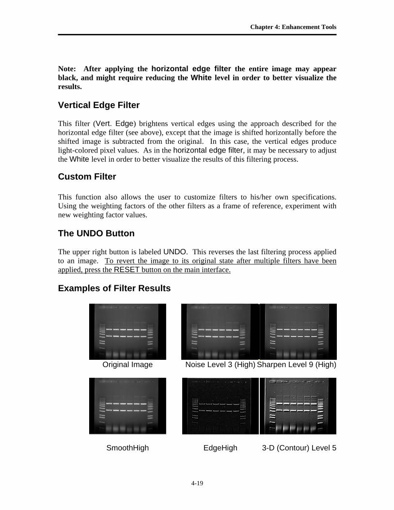
Chapter 4: Enhancement Tools
4-19
Note: After applying the horizontal edge filter the entire image may appear black, and might require reducing the White level in order to better visualize the results. Vertical Edge Filter This filter (Vert. Edge) brightens vertical edges using the approach described for the horizontal edge filter (see above), except that the image is shifted horizontally before the shifted image is subtracted from the original. In this case, the vertical edges produce light-colored pixel values. As in the horizontal edge filter, it may be necessary to adjust the White level in order to better visualize the results of this filtering process.
Custom Filter This function also allows the user to customize filters to his/her own specifications. Using the weighting factors of the other filters as a frame of reference, experiment with new weighting factor values. The UNDO Button The upper right button is labeled UNDO. This reverses the last filtering process applied to an image. To revert the image to its original state after multiple filters have been applied, press the RESET button on the main interface. Examples of Filter Results
Original Image Noise Level 3 (High) Sharpen Level 9 (High)
SmoothHigh EdgeHigh 3-D (Contour) Level 5
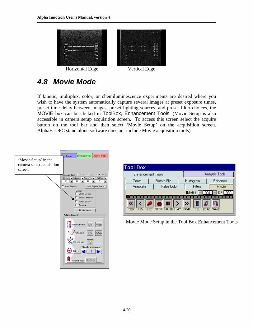
Alpha Innotech User’s Manual, version 4
4-20
Horizontal Edge Vertical Edge 4.8 Movie Mode If kinetic, multiplex, color, or chemiluminescence experiments are desired where you wish to have the system automatically capture several images at preset exposure times, preset time delay between images, preset lighting sources, and preset filter choices, the MOVIE box can be clicked in ToolBox, Enhancement Tools. (Movie Setup is also accessible in camera setup acquisition screen. To access this screen select the acquire button on the tool bar and then select ‘Movie Setup’ on the acquisition screen. AlphaEaseFC stand alone software does not include Movie acquisition tools)
‘Movie Setup’ in the camera setup acquisition screen
Movie Mode Setup in the Tool Box Enhancement Tools
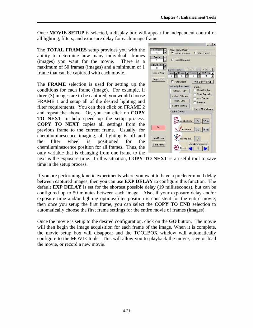
Chapter 4: Enhancement Tools
4-21
Once MOVIE SETUP is selected, a display box will appear for independent control of all lighting, filters, and exposure delay for each image frame. The TOTAL FRAMES setup provides you with the ability to determine how many individual frames (images) you want for the movie. There is a maximum of 50 frames (images) and a minimum of 1 frame that can be captured with each movie. The FRAME selection is used for setting up the conditions for each frame (image). For example, if three (3) images are to be captured, you would choose FRAME 1 and setup all of the desired lighting and filter requirements. You can then click on FRAME 2 and repeat the above. Or, you can click on COPY TO NEXT to help speed up the setup process. COPY TO NEXT copies all settings from the previous frame to the current frame. Usually, for chemiluminescence imaging, all lighting is off and the filter wheel is positioned for the chemiluminescence position for all frames. Thus, the only variable that is changing from one frame to the next is the exposure time. In this situation, COPY TO NEXT is a useful tool to save time in the setup process. If you are performing kinetic experiments where you want to have a predetermined delay between captured images, then you can use EXP DELAY to configure this function. The default EXP DELAY is set for the shortest possible delay (19 milliseconds), but can be configured up to 50 minutes between each image. Also, if your exposure delay and/or exposure time and/or lighting options/filter position is consistent for the entire movie, then once you setup the first frame, you can select the COPY TO END selection to automatically choose the first frame settings for the entire movie of frames (images). Once the movie is setup to the desired configuration, click on the GO button. The movie will then begin the image acquisition for each frame of the image. When it is complete, the movie setup box will disappear and the TOOLBOX window will automatically configure to the MOVIE tools. This will allow you to playback the movie, save or load the movie, or record a new movie.
Alpha Innotech User’s Manual, version 4
4-22
Once all images have been captured, the above Movie display box will become displayed. The remaining buttons will perform the following tasks: REC Move to Camera Setup and Preview, Movie Record setup
functions to record a movie. PLAY Display a continuous loop ‘movie’ of all of the captured images. STOP Stop the movie at the current frame display PAUSE Pause the playback of the movie at a user defined image REW (rewind) Rewind the movie to the first image REV (reverse) Play the movie in a continuous loop in reverse
FWD (forward) Forward the movie to the last image DEL (delete) Delete the movie on the display. THIS FUNCTION WILL NOT
DELETE A MOVIE SAVED TO THE HARD DRIVE. LOAD Load a previously saved movie. THIS FUNCTION WILL NOT
LOAD INDIVIDUAL IMAGES PREVIOUSLY CAPTURED IN NORMAL CAPTURE MODE.
SAVE Save a movie of images. Saving An Individual Image From a Movie After you load, play, and stop a movie at the desired image, it is possible to save the individual image seen on the screen. Use the SAVE AS button located on the tool bar to save the image in the desired location and file format on the local or network drives.
Note: This will save the current image only. To save the entire movie, select the ‘save’ icon on the movie tab in the enhancement tools.
Loading/Saving an Entire Movie
You can load or save an entire movie by using the load and save icons in the movie tab in the enhancement tools. When a movie is loaded the loaded frames will be seen as blue in the movie reel. When a movie is saved a dialog
box will appear prompting you to select the location and name for the movie that you would like to save the images as.
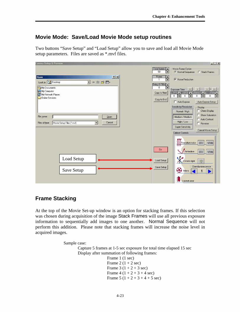
Chapter 4: Enhancement Tools
4-23
Movie Mode: Save/Load Movie Mode setup routines Two buttons “Save Setup” and “Load Setup” allow you to save and load all Movie Mode setup parameters. Files are saved as *.mvf files.
Frame Stacking At the top of the Movie Set-up window is an option for stacking frames. If this selection was chosen during acquisition of the image Stack Frames will use all previous exposure information to sequentially add images to one another. Normal Sequence will not perform this addition. Please note that stacking frames will increase the noise level in acquired images. Sample case: Capture 5 frames at 1-5 sec exposure for total time elapsed 15 sec Display after summation of following frames:
Frame 1 (1 sec) Frame 2 (1 + 2 sec) Frame 3 (1 + 2 + 3 sec) Frame 4 (1 + 2 + 3 + 4 sec)
Frame 5 (1 + 2 + 3 + 4 + 5 sec)
Load Setup
Save Setup
Alpha Innotech User’s Manual, version 4
4-24
Capturing a Color Image Using the Movie Function A color image can be generated by acquiring three images each taken with a red, green and blue emission filter. Once saved, these images are then combined in the Overlay pull down menu. Open the image captured with each of the three filters as instructed and a RGB (red, green, blue) true color image will be generated. For color imaging, you will need to the following optional filters:
Red Filter SYPRO Red Filter
Blue Filter Hoechst Blue Filter
Green Filter SYBR Green Filter
Note: For multiplexing with 2 different fluorescent stains, you will need the optional AIC filters designed for each stain.

Chapter 4: Enhancement Tools
4-25
BLANK PAGE

Alpha Innotech User’s Manual, version 4
4-26
BLANK PAGE
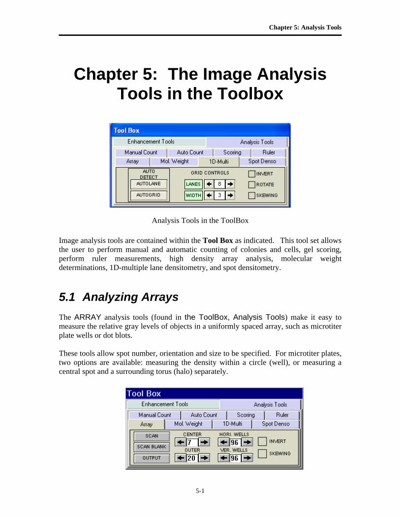
Chapter 5: Analysis Tools
5-1
Chapter 5: The Image Analysis Tools in the Toolbox
Analysis Tools in the ToolBox Image analysis tools are contained within the Tool Box as indicated. This tool set allows the user to perform manual and automatic counting of colonies and cells, gel scoring, perform ruler measurements, high density array analysis, molecular weight determinations, 1D-multiple lane densitometry, and spot densitometry. 5.1 Analyzing Arrays The ARRAY analysis tools (found in the ToolBox, Analysis Tools) make it easy to measure the relative gray levels of objects in a uniformly spaced array, such as microtiter plate wells or dot blots. These tools allow spot number, orientation and size to be specified. For microtiter plates, two options are available: measuring the density within a circle (well), or measuring a central spot and a surrounding torus (halo) separately.
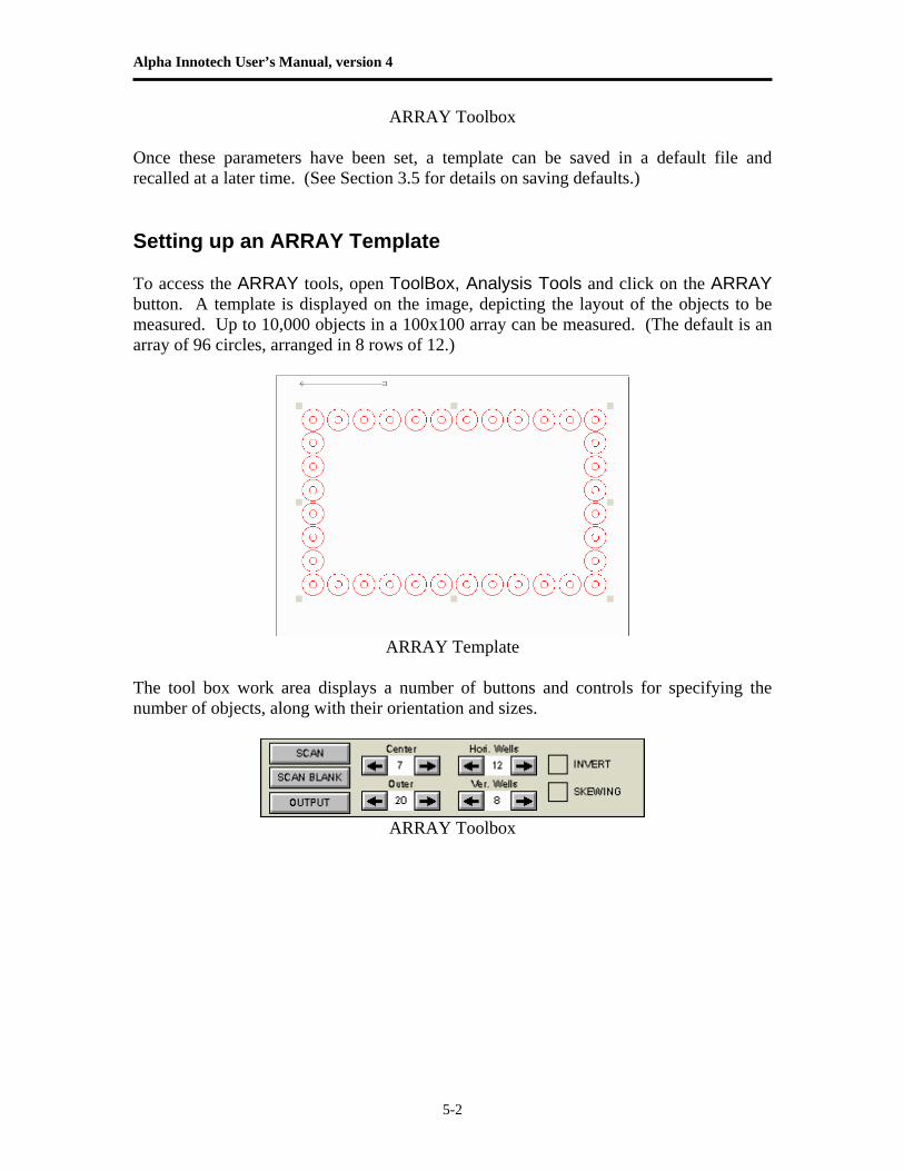
Alpha Innotech User’s Manual, version 4
5-2
ARRAY Toolbox Once these parameters have been set, a template can be saved in a default file and recalled at a later time. (See Section 3.5 for details on saving defaults.) Setting up an ARRAY Template To access the ARRAY tools, open ToolBox, Analysis Tools and click on the ARRAY button. A template is displayed on the image, depicting the layout of the objects to be measured. Up to 10,000 objects in a 100x100 array can be measured. (The default is an array of 96 circles, arranged in 8 rows of 12.)
ARRAY Template
The tool box work area displays a number of buttons and controls for specifying the number of objects, along with their orientation and sizes.
ARRAY Toolbox
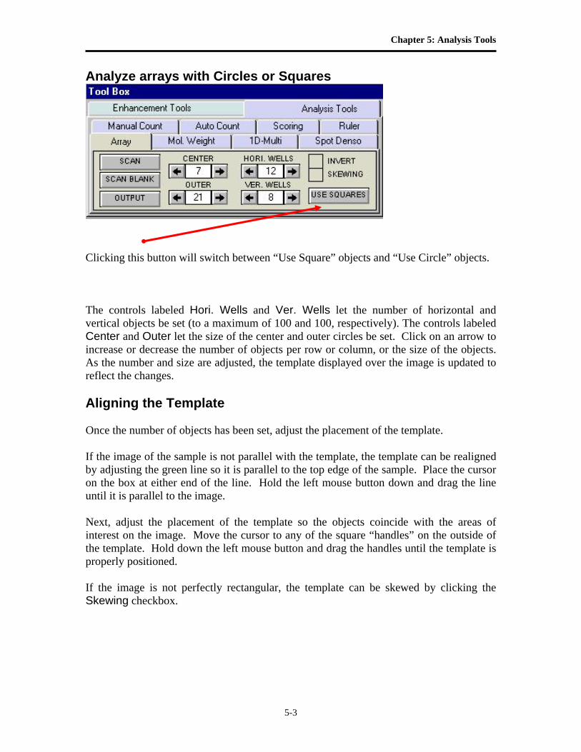
Chapter 5: Analysis Tools
5-3
Analyze arrays with Circles or Squares
Clicking this button will switch between “Use Square” objects and “Use Circle” objects. The controls labeled Hori. Wells and Ver. Wells let the number of horizontal and vertical objects be set (to a maximum of 100 and 100, respectively). The controls labeled Center and Outer let the size of the center and outer circles be set. Click on an arrow to increase or decrease the number of objects per row or column, or the size of the objects. As the number and size are adjusted, the template displayed over the image is updated to reflect the changes. Aligning the Template Once the number of objects has been set, adjust the placement of the template. If the image of the sample is not parallel with the template, the template can be realigned by adjusting the green line so it is parallel to the top edge of the sample. Place the cursor on the box at either end of the line. Hold the left mouse button down and drag the line until it is parallel to the image. Next, adjust the placement of the template so the objects coincide with the areas of interest on the image. Move the cursor to any of the square “handles” on the outside of the template. Hold down the left mouse button and drag the handles until the template is properly positioned. If the image is not perfectly rectangular, the template can be skewed by clicking the Skewing checkbox.
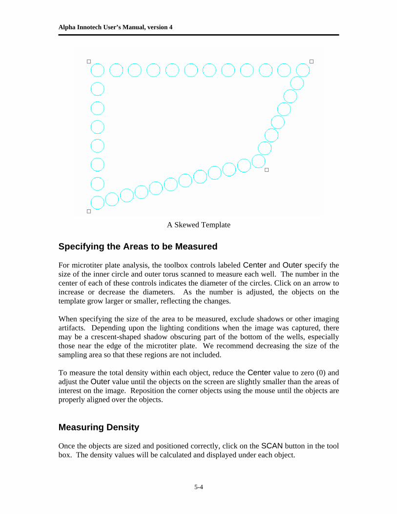
Alpha Innotech User’s Manual, version 4
5-4
A Skewed Template
Specifying the Areas to be Measured For microtiter plate analysis, the toolbox controls labeled Center and Outer specify the size of the inner circle and outer torus scanned to measure each well. The number in the center of each of these controls indicates the diameter of the circles. Click on an arrow to increase or decrease the diameters. As the number is adjusted, the objects on the template grow larger or smaller, reflecting the changes. When specifying the size of the area to be measured, exclude shadows or other imaging artifacts. Depending upon the lighting conditions when the image was captured, there may be a crescent-shaped shadow obscuring part of the bottom of the wells, especially those near the edge of the microtiter plate. We recommend decreasing the size of the sampling area so that these regions are not included. To measure the total density within each object, reduce the Center value to zero (0) and adjust the Outer value until the objects on the screen are slightly smaller than the areas of interest on the image. Reposition the corner objects using the mouse until the objects are properly aligned over the objects. Measuring Density Once the objects are sized and positioned correctly, click on the SCAN button in the tool box. The density values will be calculated and displayed under each object.
Chapter 5: Analysis Tools
5-5
The values are the average pixel values within the object, adjusted to a scale of 0 to 100. (0 corresponding to black pixel values, and 100 corresponding to white pixel values.) If both a center and an outer circle have been specified, two values are displayed. The upper value corresponds to the inner circle and the lower value corresponds to the torus. The INVERT Box The INVERT function reverses the relative density assignments so that 0 corresponds to white and 100 corresponds to black. If the image has dark areas of interest on a light background, then INVERT should be selected by placing an “X” in its box. (If the image has light areas of interest on a dark background, the INVERT option should not be activated.) Unlike the REVERSE button described in Chapter 3, this function does not alter the appearance of the image. Removing Background using the Scan Blank Function Since a microtiter plate is not completely transparent, it contributes to the density measured when samples are scanned. A non-uniform light source also affects the density measured. To ensure that the density measured is attributable only to the sample in the wells, scan a “blank” before scanning samples. Load an image of a clean, unused microtiter plate and align the objects as described above. Once the array has been set up, click on the Scan Blank button. The average pixel gray value for each object (and torus) is measured and set to zero (0). Now, when samples are scanned, the gray value of the blank is subtracted from that of the sample before it is scaled. This ensures that the density reported only reflects the sample in each well. When Scan Blank has been selected, the background values obtained apply to all subsequent scans. To indicate that a background is being applied, the Scan Blank button changes to read Clear Blank. To turn off this background subtraction function, simply click on Clear Blank. Outputting Data The Output button outputs data as a hard copy or as an ASCII text file which can then be imported into a spreadsheet for further analysis and/or graphing.
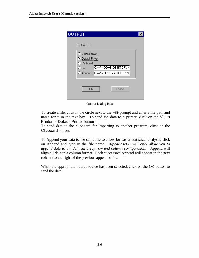
Alpha Innotech User’s Manual, version 4
5-6
Output Dialog Box
To create a file, click in the circle next to the File prompt and enter a file path and name for it in the text box. To send the data to a printer, click on the Video Printer or Default Printer buttons. To send data to the clipboard for importing to another program, click on the Clipboard button. To Append your data to the same file to allow for easier statistical analysis, click on Append and type in the file name. AlphaEaseFC will only allow you to append data to an identical array row and column configuration. Append will align all data in a column format. Each successive Append will appear in the next column to the right of the previous appended file. When the appropriate output source has been selected, click on the OK button to send the data.
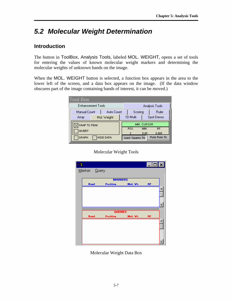
Chapter 5: Analysis Tools
5-7
5.2 Molecular Weight Determination
Introduction The button in ToolBox, Analysis Tools, labeled MOL. WEIGHT, opens a set of tools for entering the values of known molecular weight markers and determining the molecular weights of unknown bands on the image. When the MOL. WEIGHT button is selected, a function box appears in the area to the lower left of the screen, and a data box appears on the image. (If the data window obscures part of the image containing bands of interest, it can be moved.)
Molecular Weight Tools
Molecular Weight Data Box
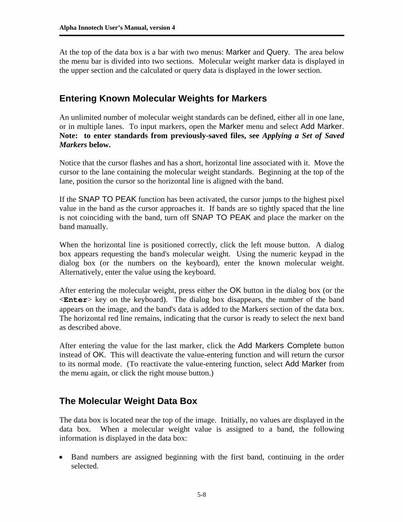
Alpha Innotech User’s Manual, version 4
5-8
At the top of the data box is a bar with two menus: Marker and Query. The area below the menu bar is divided into two sections. Molecular weight marker data is displayed in the upper section and the calculated or query data is displayed in the lower section. Entering Known Molecular Weights for Markers An unlimited number of molecular weight standards can be defined, either all in one lane, or in multiple lanes. To input markers, open the Marker menu and select Add Marker. Note: to enter standards from previously-saved files, see Applying a Set of Saved Markers below. Notice that the cursor flashes and has a short, horizontal line associated with it. Move the cursor to the lane containing the molecular weight standards. Beginning at the top of the lane, position the cursor so the horizontal line is aligned with the band. If the SNAP TO PEAK function has been activated, the cursor jumps to the highest pixel value in the band as the cursor approaches it. If bands are so tightly spaced that the line is not coinciding with the band, turn off SNAP TO PEAK and place the marker on the band manually. When the horizontal line is positioned correctly, click the left mouse button. A dialog box appears requesting the band's molecular weight. Using the numeric keypad in the dialog box (or the numbers on the keyboard), enter the known molecular weight. Alternatively, enter the value using the keyboard. After entering the molecular weight, press either the OK button in the dialog box (or the <Enter> key on the keyboard). The dialog box disappears, the number of the band appears on the image, and the band's data is added to the Markers section of the data box. The horizontal red line remains, indicating that the cursor is ready to select the next band as described above. After entering the value for the last marker, click the Add Markers Complete button instead of OK. This will deactivate the value-entering function and will return the cursor to its normal mode. (To reactivate the value-entering function, select Add Marker from the menu again, or click the right mouse button.) The Molecular Weight Data Box The data box is located near the top of the image. Initially, no values are displayed in the data box. When a molecular weight value is assigned to a band, the following information is displayed in the data box: • Band numbers are assigned beginning with the first band, continuing in the order
selected.
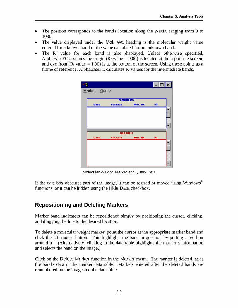
Chapter 5: Analysis Tools
5-9
• The position corresponds to the band's location along the y-axis, ranging from 0 to 1030.
• The value displayed under the Mol. Wt. heading is the molecular weight value entered for a known band or the value calculated for an unknown band.
• The Rf value for each band is also displayed. Unless otherwise specified, AlphaEaseFC assumes the origin (Rf value = 0.00) is located at the top of the screen, and dye front (Rf value = 1.00) is at the bottom of the screen. Using these points as a frame of reference, AlphaEaseFC calculates Rf values for the intermediate bands.
Molecular Weight Marker and Query Data If the data box obscures part of the image, it can be resized or moved using Windows® functions, or it can be hidden using the Hide Data checkbox. Repositioning and Deleting Markers Marker band indicators can be repositioned simply by positioning the cursor, clicking, and dragging the line to the desired location. To delete a molecular weight marker, point the cursor at the appropriate marker band and click the left mouse button. This highlights the band in question by putting a red box around it. (Alternatively, clicking in the data table highlights the marker’s information and selects the band on the image.) Click on the Delete Marker function in the Marker menu. The marker is deleted, as is the band's data in the marker data table. Markers entered after the deleted bands are renumbered on the image and the data table.
Alpha Innotech User’s Manual, version 4
5-10
To delete all the markers and start over, select the Clear Markers function in the Marker menu. Determining Molecular Weights of Unknown Bands After marker values are entered, the molecular weight of any unknown band can be determined.
Manually Selecting Bands To indicate unknown bands manually, select the Add Band function from the Query menu. Just as in Add Marker above, a line will appear attached to the cursor. Point the cursor at the band of interest and click the mouse button. The molecular weight of the band is automatically calculated and displayed in the Queries section of the data box. To select a second band, click the right mouse button and the cursor line will reappear. Repeat this procedure for all bands for which molecular weights is to be determined. Note that the molecular weight markers appear in blue while the queries appear in green. The molecular weight of a band is calculated based on the graph of the known marker bands. (Note: If a query band lies outside of the markers, it will be extrapolated in “Least Squares Fit” mode or given a value of “N/A” in “Point-to-Point” mode.) See The Graph Tool below for more information.
Automatic Band Finding AlphaEaseFC includes an algorithm for automatically finding bands in query lanes. To use this function, select Auto Query from the Query menu. A yellow vertical line will appear attached to the cursor. Position the line over the lane of interest and click the left mouse button. The bands in the lanes will be selected automatically, and their data will appear in the Data box.
Repositioning and Deleting Bands Bands can be repositioned simply by positioning the cursor, clicking, and dragging the band to the desired location.
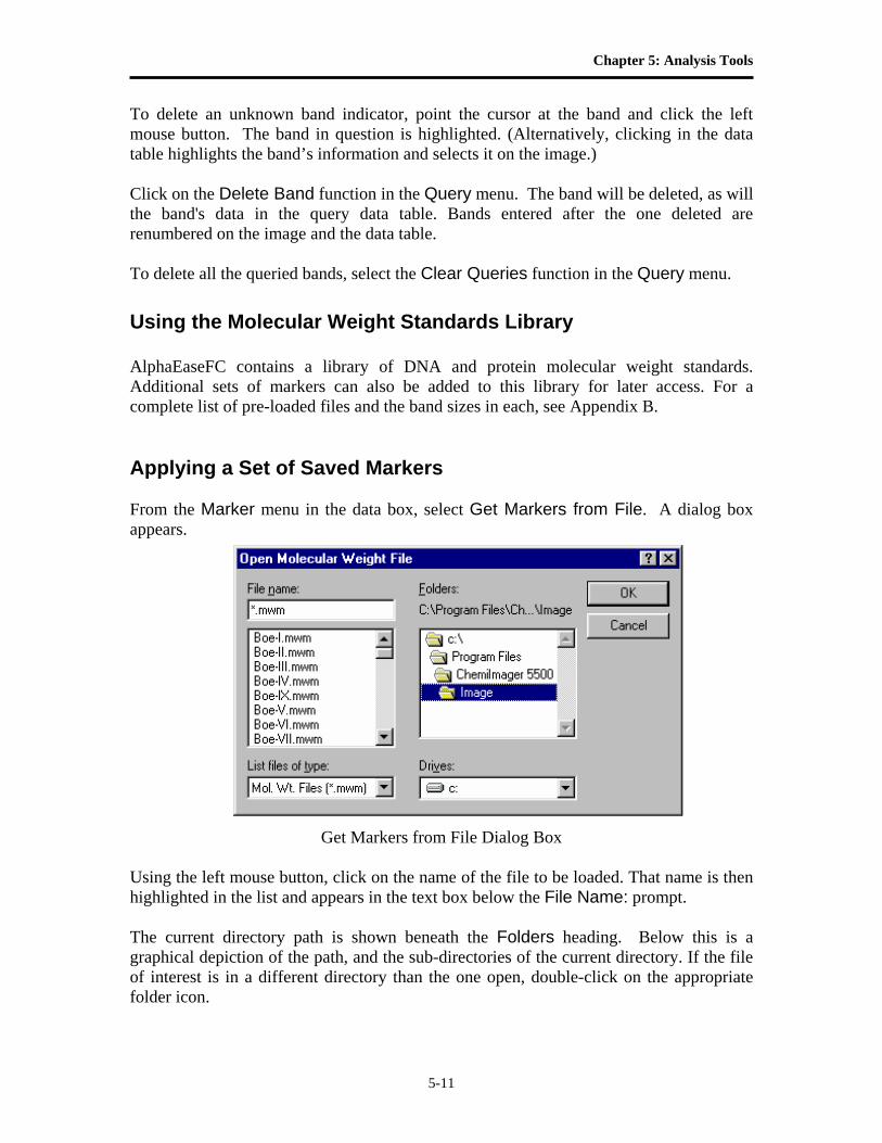
Chapter 5: Analysis Tools
5-11
To delete an unknown band indicator, point the cursor at the band and click the left mouse button. The band in question is highlighted. (Alternatively, clicking in the data table highlights the band’s information and selects it on the image.) Click on the Delete Band function in the Query menu. The band will be deleted, as will the band's data in the query data table. Bands entered after the one deleted are renumbered on the image and the data table. To delete all the queried bands, select the Clear Queries function in the Query menu. Using the Molecular Weight Standards Library AlphaEaseFC contains a library of DNA and protein molecular weight standards. Additional sets of markers can also be added to this library for later access. For a complete list of pre-loaded files and the band sizes in each, see Appendix B. Applying a Set of Saved Markers From the Marker menu in the data box, select Get Markers from File. A dialog box appears.
Get Markers from File Dialog Box Using the left mouse button, click on the name of the file to be loaded. That name is then highlighted in the list and appears in the text box below the File Name: prompt. The current directory path is shown beneath the Folders heading. Below this is a graphical depiction of the path, and the sub-directories of the current directory. If the file of interest is in a different directory than the one open, double-click on the appropriate folder icon.
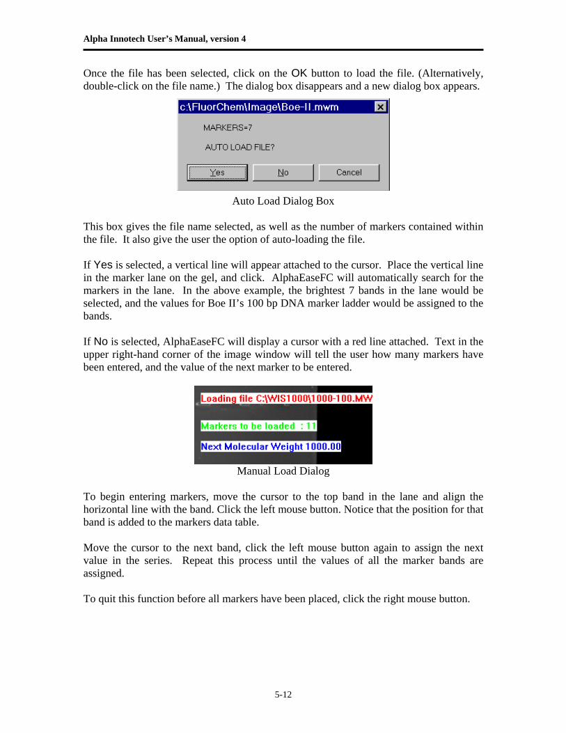
Alpha Innotech User’s Manual, version 4
5-12
Once the file has been selected, click on the OK button to load the file. (Alternatively, double-click on the file name.) The dialog box disappears and a new dialog box appears.
Auto Load Dialog Box This box gives the file name selected, as well as the number of markers contained within the file. It also give the user the option of auto-loading the file. If Yes is selected, a vertical line will appear attached to the cursor. Place the vertical line in the marker lane on the gel, and click. AlphaEaseFC will automatically search for the markers in the lane. In the above example, the brightest 7 bands in the lane would be selected, and the values for Boe II’s 100 bp DNA marker ladder would be assigned to the bands. If No is selected, AlphaEaseFC will display a cursor with a red line attached. Text in the upper right-hand corner of the image window will tell the user how many markers have been entered, and the value of the next marker to be entered.
Manual Load Dialog
To begin entering markers, move the cursor to the top band in the lane and align the horizontal line with the band. Click the left mouse button. Notice that the position for that band is added to the markers data table. Move the cursor to the next band, click the left mouse button again to assign the next value in the series. Repeat this process until the values of all the marker bands are assigned. To quit this function before all markers have been placed, click the right mouse button.
Chapter 5: Analysis Tools
5-13
Adding a Set of Molecular Weight Markers to the Library If the same set of molecular weight markers will be run repeatedly, there is no need to enter values on each new image. Instead, save the molecular weight values in a file and apply them to the marker lane of any subsequent images. To save a set of molecular weight standards, click on Write Markers to File in the Marker menu after the marker values have been entered. Following Windows conventions (255 characters or less), enter a new file name in the text box below the File Name: prompt. AlphaEaseFC will automatically give the appropriate 3-character extension. The current directory path is shown beneath the Directories heading. Below this is a graphical depiction of the path, and the sub-directories of the current directory. If the file is to be saved in a different directory than the one open, double-click on the appropriate folder icon. Alternate disk drives can be accessed using the Drives heading. Once a name has been entered and the appropriate directory has been accessed, click OK. All of the marker values that are currently in the Data window will be saved to this new file. To access them in the future, follow the steps in Applying a Set of Saved Markers above. Outputting Data The Output function in the Query menu outputs data as a hard copy or as an ASCII text file which can then be imported into a spreadsheet for further analysis and/or graphing.

Alpha Innotech User’s Manual, version 4
5-14
Output Dialog Box To create a file, click in the box next to the File prompt and enter a path and file name for it in the text box. To send the data to a printer, click on the Video Printer or Default Printer buttons. To send data to the clipboard for importing to another program, click on the Clipboard button. When the appropriate output source has been selected, click on the OK button to send the data. Special Functions: Snap to Peak This feature makes it easier to place the cursor on a band. If the SNAP TO PEAK function has been activated, the cursor jumps to the highest pixel value in the band as the cursor approaches it. If bands are so tightly spaced that the line is not coinciding with the band, turn off SNAP TO PEAK and place the marker on the band manually. If the cursor is jumping to areas between bands instead of the bands themselves, check to see that INVERT is properly set. (See below for more information.) The INVERT Button The INVERT function reverses the gray scale assignments so that 0 corresponds to white and 4,095 corresponds to black. If the image has dark bands and light background, then INVERT should be selected by placing an “X” in its box. (If the image has light bands and dark background, the INVERT option should not be activated.) Unlike the
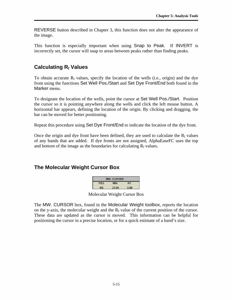
Chapter 5: Analysis Tools
5-15
REVERSE button described in Chapter 3, this function does not alter the appearance of the image. This function is especially important when using Snap to Peak. If INVERT is incorrectly set, the cursor will snap to areas between peaks rather than finding peaks. Calculating Rf Values To obtain accurate Rf values, specify the location of the wells (i.e., origin) and the dye front using the functions Set Well Pos./Start and Set Dye Front/End both found in the Marker menu. To designate the location of the wells, point the cursor at Set Well Pos./Start. Position the cursor so it is pointing anywhere along the wells and click the left mouse button. A horizontal bar appears, defining the location of the origin. By clicking and dragging, the bar can be moved for better positioning. Repeat this procedure using Set Dye Front/End to indicate the location of the dye front. Once the origin and dye front have been defined, they are used to calculate the Rf values of any bands that are added. If dye fronts are not assigned, AlphaEaseFC uses the top and bottom of the image as the boundaries for calculating Rf values. The Molecular Weight Cursor Box
Molecular Weight Cursor Box
The MW. CURSOR box, found in the Molecular Weight toolbox, reports the location on the y-axis, the molecular weight and the Rf value of the current position of the cursor. These data are updated as the cursor is moved. This information can be helpful for positioning the cursor in a precise location, or for a quick estimate of a band’s size.
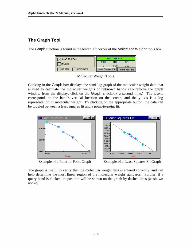
Alpha Innotech User’s Manual, version 4
5-16
The Graph Tool The Graph function is found in the lower left corner of the Molecular Weight tools box.
Molecular Weight Tools
Clicking in the Graph box displays the semi-log graph of the molecular weight data that is used to calculate the molecular weights of unknown bands. (To remove the graph window from the display, click on the Graph checkbox a second time.) The x-axis corresponds to the band's vertical location on the screen, and the y-axis is a log representation of molecular weight. By clicking on the appropriate button, the data can be toggled between a least squares fit and a point-to-point fit.
Example of a Point-to-Point Graph Example of a Least Squares Fit Graph The graph is useful to verify that the molecular weight data is entered correctly, and can help determine the most linear region of the molecular weight standards. Further, if a query band is clicked, its position will be shown on the graph by dashed lines (as shown above).
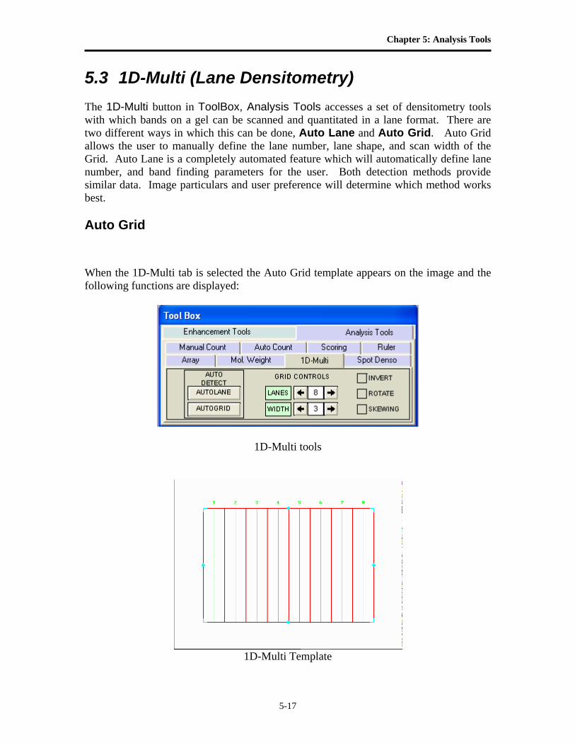
Chapter 5: Analysis Tools
5-17
5.3 1D-Multi (Lane Densitometry) The 1D-Multi button in ToolBox, Analysis Tools accesses a set of densitometry tools with which bands on a gel can be scanned and quantitated in a lane format. There are two different ways in which this can be done, Auto Lane and Auto Grid. Auto Grid allows the user to manually define the lane number, lane shape, and scan width of the Grid. Auto Lane is a completely automated feature which will automatically define lane number, and band finding parameters for the user. Both detection methods provide similar data. Image particulars and user preference will determine which method works best. Auto Grid
When the 1D-Multi tab is selected the Auto Grid template appears on the image and the following functions are displayed:
1D-Multi tools
1D-Multi Template
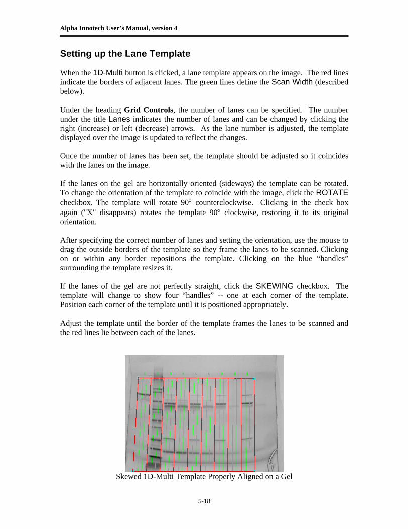
Alpha Innotech User’s Manual, version 4
5-18
Setting up the Lane Template When the 1D-Multi button is clicked, a lane template appears on the image. The red lines indicate the borders of adjacent lanes. The green lines define the Scan Width (described below). Under the heading Grid Controls, the number of lanes can be specified. The number under the title Lanes indicates the number of lanes and can be changed by clicking the right (increase) or left (decrease) arrows. As the lane number is adjusted, the template displayed over the image is updated to reflect the changes. Once the number of lanes has been set, the template should be adjusted so it coincides with the lanes on the image. If the lanes on the gel are horizontally oriented (sideways) the template can be rotated. To change the orientation of the template to coincide with the image, click the ROTATE checkbox. The template will rotate 90° counterclockwise. Clicking in the check box again ("X" disappears) rotates the template 90° clockwise, restoring it to its original orientation. After specifying the correct number of lanes and setting the orientation, use the mouse to drag the outside borders of the template so they frame the lanes to be scanned. Clicking on or within any border repositions the template. Clicking on the blue “handles” surrounding the template resizes it. If the lanes of the gel are not perfectly straight, click the SKEWING checkbox. The template will change to show four “handles” -- one at each corner of the template. Position each corner of the template until it is positioned appropriately. Adjust the template until the border of the template frames the lanes to be scanned and the red lines lie between each of the lanes.
Skewed 1D-Multi Template Properly Aligned on a Gel
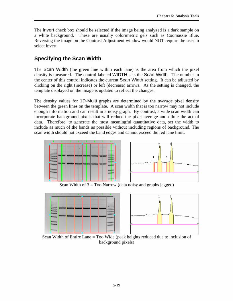
Chapter 5: Analysis Tools
5-19
The Invert check box should be selected if the image being analyzed is a dark sample on a white background. These are usually colorimetric gels such as Coomassie Blue. Reversing the image on the Contrast Adjustment window would NOT require the user to select invert. Specifying the Scan Width The Scan Width (the green line within each lane) is the area from which the pixel density is measured. The control labeled WIDTH sets the Scan Width. The number in the center of this control indicates the current Scan Width setting. It can be adjusted by clicking on the right (increase) or left (decrease) arrows. As the setting is changed, the template displayed on the image is updated to reflect the changes. The density values for 1D-Multi graphs are determined by the average pixel density between the green lines on the template. A scan width that is too narrow may not include enough information and can result in a noisy graph. By contrast, a wide scan width can incorporate background pixels that will reduce the pixel average and dilute the actual data. Therefore, to generate the most meaningful quantitative data, set the width to include as much of the bands as possible without including regions of background. The scan width should not exceed the band edges and cannot exceed the red lane limit.
Scan Width of 3 = Too Narrow (data noisy and graphs jagged)
Scan Width of Entire Lane = Too Wide (peak heights reduced due to inclusion of
background pixels)

Alpha Innotech User’s Manual, version 4
5-20
Recommended Scan Width (middle of bands scanned; “smiling” edges excluded)
Scanning the Image When the AUTOGRID button is clicked, the densities of each lane are measured, and information is displayed in several quadrants of the screen: • The graphs for each lane scanned are displayed in the lower left. • The active graph is displayed in the upper quadrant of the screen. • Peak information for the active graph is displayed in a data table in the lower right. • The Image is displayed behind the above windows and can be viewed by reducing the
individual display windows.
Image Area of Sample Scan
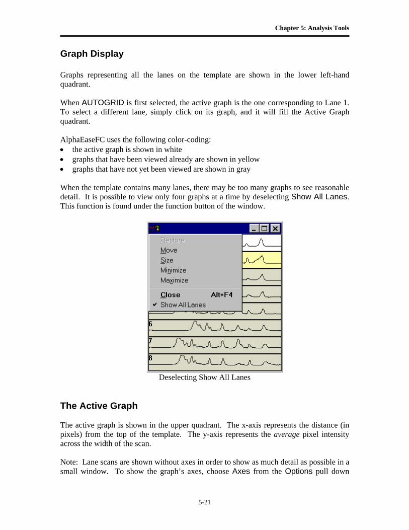
Chapter 5: Analysis Tools
5-21
Graph Display Graphs representing all the lanes on the template are shown in the lower left-hand quadrant. When AUTOGRID is first selected, the active graph is the one corresponding to Lane 1. To select a different lane, simply click on its graph, and it will fill the Active Graph quadrant. AlphaEaseFC uses the following color-coding: • the active graph is shown in white • graphs that have been viewed already are shown in yellow • graphs that have not yet been viewed are shown in gray When the template contains many lanes, there may be too many graphs to see reasonable detail. It is possible to view only four graphs at a time by deselecting Show All Lanes. This function is found under the function button of the window.
Deselecting Show All Lanes The Active Graph The active graph is shown in the upper quadrant. The x-axis represents the distance (in pixels) from the top of the template. The y-axis represents the average pixel intensity across the width of the scan. Note: Lane scans are shown without axes in order to show as much detail as possible in a small window. To show the graph’s axes, choose Axes from the Options pull down
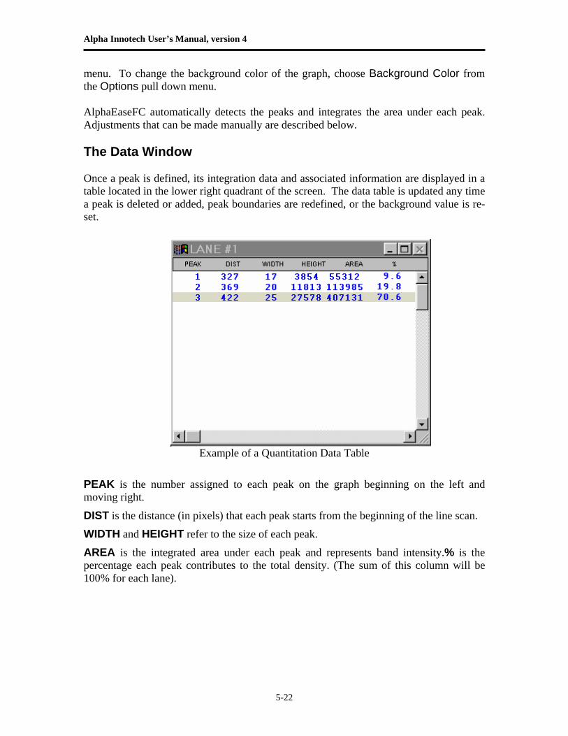
Alpha Innotech User’s Manual, version 4
5-22
menu. To change the background color of the graph, choose Background Color from the Options pull down menu. AlphaEaseFC automatically detects the peaks and integrates the area under each peak. Adjustments that can be made manually are described below. The Data Window Once a peak is defined, its integration data and associated information are displayed in a table located in the lower right quadrant of the screen. The data table is updated any time a peak is deleted or added, peak boundaries are redefined, or the background value is re-set.
Example of a Quantitation Data Table PEAK is the number assigned to each peak on the graph beginning on the left and moving right.
DIST is the distance (in pixels) that each peak starts from the beginning of the line scan.
WIDTH and HEIGHT refer to the size of each peak.
AREA is the integrated area under each peak and represents band intensity.% is the percentage each peak contributes to the total density. (The sum of this column will be 100% for each lane).
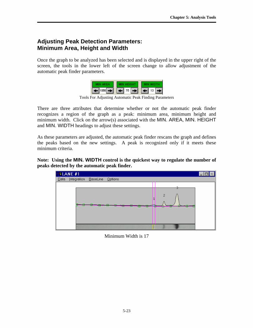
Chapter 5: Analysis Tools
5-23
Adjusting Peak Detection Parameters: Minimum Area, Height and Width Once the graph to be analyzed has been selected and is displayed in the upper right of the screen, the tools in the lower left of the screen change to allow adjustment of the automatic peak finder parameters.
Tools For Adjusting Automatic Peak Finding Parameters
There are three attributes that determine whether or not the automatic peak finder recognizes a region of the graph as a peak: minimum area, minimum height and minimum width. Click on the arrow(s) associated with the MIN. AREA, MIN. HEIGHT and MIN. WIDTH headings to adjust these settings. As these parameters are adjusted, the automatic peak finder rescans the graph and defines the peaks based on the new settings. A peak is recognized only if it meets these minimum criteria. Note: Using the MIN. WIDTH control is the quickest way to regulate the number of peaks detected by the automatic peak finder.
Minimum Width is 17
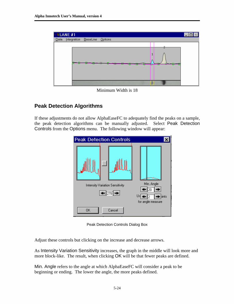
Alpha Innotech User’s Manual, version 4
5-24
Minimum Width is 18
Peak Detection Algorithms If these adjustments do not allow AlphaEaseFC to adequately find the peaks on a sample, the peak detection algorithms can be manually adjusted. Select Peak Detection Controls from the Options menu. The following window will appear:
Peak Detection Controls Dialog Box
Adjust these controls but clicking on the increase and decrease arrows. As Intensity Variation Sensitivity increases, the graph in the middle will look more and more block-like. The result, when clicking OK will be that fewer peaks are defined. Min. Angle refers to the angle at which AlphaEaseFC will consider a peak to be beginning or ending. The lower the angle, the more peaks defined.
Chapter 5: Analysis Tools
5-25
Use points for angle measure refers to the number of data points that will be scanned at once to determine an angle. The larger the number of points, the less sensitive the algorithm (ie. the fewer peaks that will be defined). Editing Peaks: Editing Peak Boundaries The boundaries of existing peaks can be readjusted to make the peaks wider or narrower. To adjust either peak boundary, click on the peak to select it. Next, point the cursor at the vertical boundary line, hold down the left mouse button and drag the line to the desired location. When it is in place, release the mouse button. The data table is automatically updated to reflect any adjustments. Both the peak and the data in the data table will be blue to indicate that this is a user-defined (vs. automatically detected) peak.
Manually Adding Peaks Additional peaks can be defined manually using the Add Peak function (in the Integration menu). When this function is selected, a vertical line appears. Position the vertical line so it corresponds to the left edge of the peak, click the left mouse button to define the left boundary of the peak, then move the cursor to the right edge of the peak and click again to define the right boundary. The peak area between the 2 limits now appears shaded, and the data table is automatically updated. Both the peak and the data in the data table will be blue to indicate that this is a user-defined (vs. automatically detected) peak. To define a second peak, click the right mouse button to reactivate the cursor.
Deleting Peaks A peak can be deleted by clicking on the peak and selecting Remove Peak from the Integration menu. The selected peak's integration disappears, and the integrated peaks to the right are renumbered accordingly. A peak can also be deleted by clicking on its entry in the data table window and hitting the <Delete> key on the keyboard. To prevent accidental deletions, a dialog box will open, asking for confirmation.
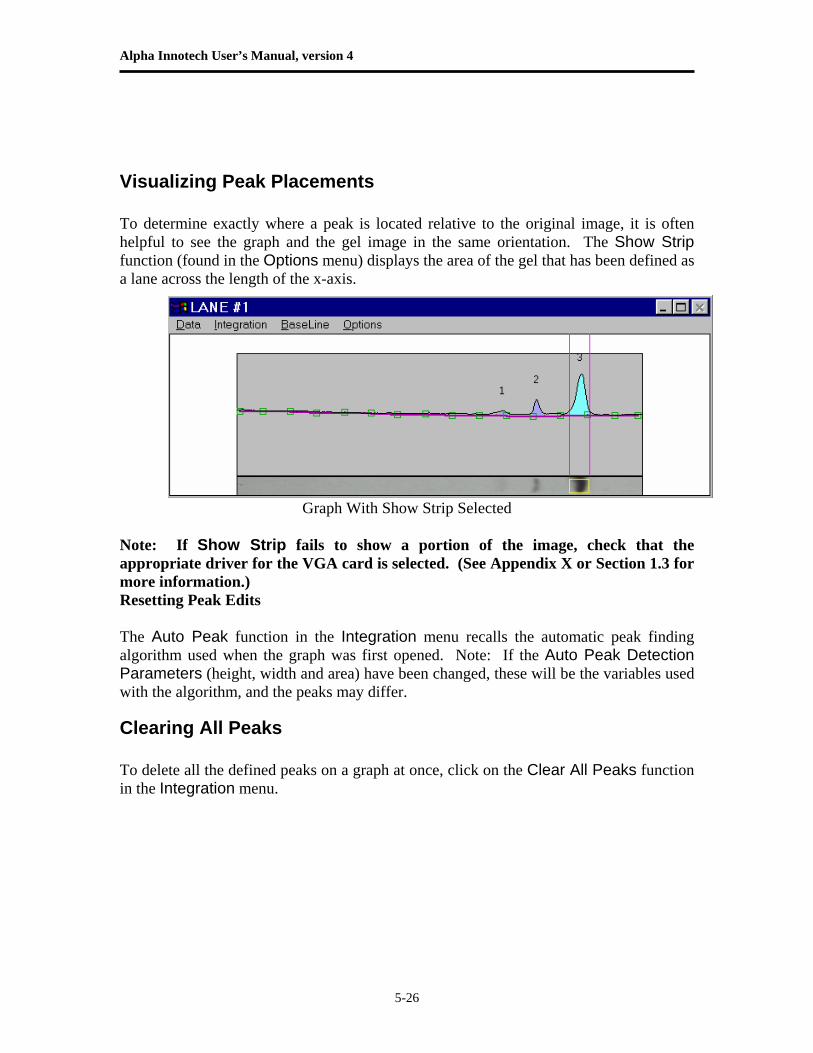
Alpha Innotech User’s Manual, version 4
5-26
Visualizing Peak Placements To determine exactly where a peak is located relative to the original image, it is often helpful to see the graph and the gel image in the same orientation. The Show Strip function (found in the Options menu) displays the area of the gel that has been defined as a lane across the length of the x-axis.
Graph With Show Strip Selected Note: If Show Strip fails to show a portion of the image, check that the appropriate driver for the VGA card is selected. (See Appendix X or Section 1.3 for more information.) Resetting Peak Edits The Auto Peak function in the Integration menu recalls the automatic peak finding algorithm used when the graph was first opened. Note: If the Auto Peak Detection Parameters (height, width and area) have been changed, these will be the variables used with the algorithm, and the peaks may differ.
Clearing All Peaks To delete all the defined peaks on a graph at once, click on the Clear All Peaks function in the Integration menu.
Chapter 5: Analysis Tools
5-27
Adjusting the Baseline: As a default, the baseline value is set to Auto Base. As the baseline is adjusted, the values for all peaks are updated to reflect the new baseline. All of the following functions are found in the Background Subtraction menu: Auto Base This method breaks the red line defining the left boundary of the lane into sixteen regions, and outputs sixteen points which reflect the average backgrounds across those sixteen regions. The user can manipulate the 16 points by clicking and dragging. The user may also designate more points than the 16 and manipulate those in the same fashion. Intra-Lane This method uses the lower of the two values at the edges of the lane along its travel as the background. If the section of the image is used is wider than the bands, then this is a very effective way of removing co-migrating material from your measurements. This method should only be used if the bands are completely enclosed. This is because when the edges of your lane area intersect any of your bands, band material will be considered as background, severely affecting your results. Rubber Band This method can be thought of as stretching a rubber band underneath the lane profile. This option does not work well if the values at the ends of the intensity profile are lower than the rest of the intensity pixels. We do not recommend this method for images with poorly separated bands. Minimum Profile This method takes the lowest value on the profile of each lane as the background for that lane. We do not recommend this method for lanes where the beginning or end of the lane is the lowest point as this is dependent on where the lane boundary was placed when it was defined. This can be hard to repeat between analysis of the same gel. Valley to Valley
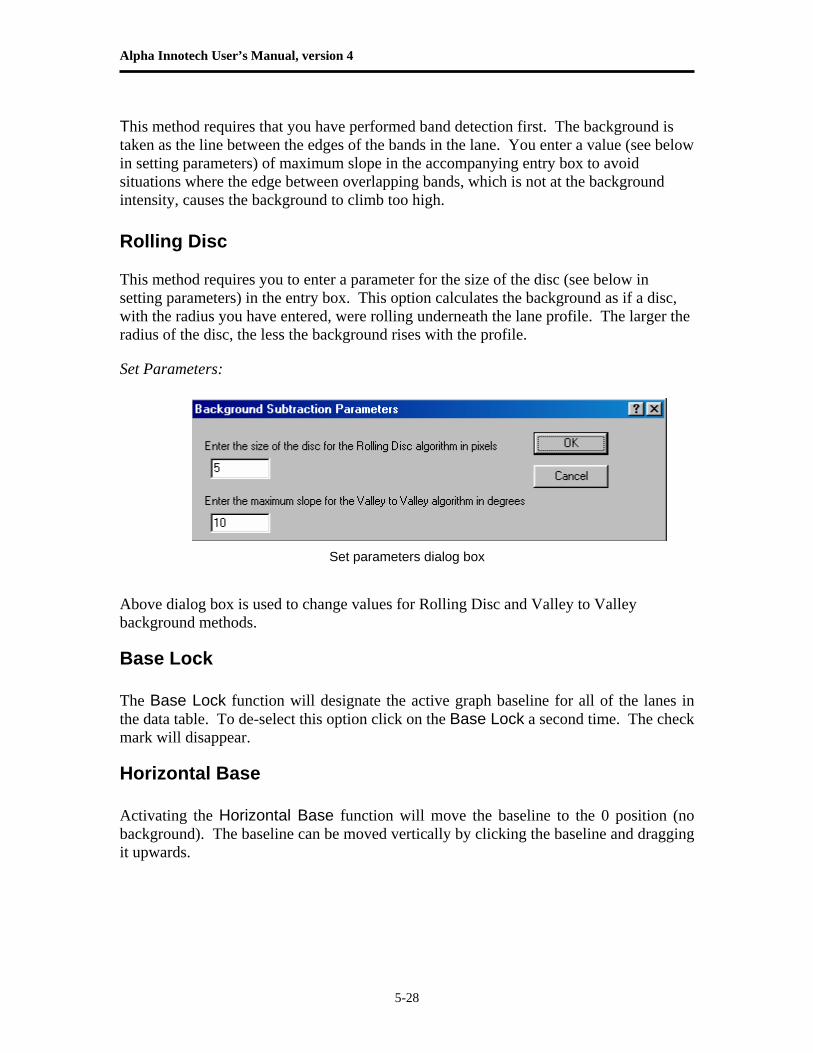
Alpha Innotech User’s Manual, version 4
5-28
This method requires that you have performed band detection first. The background is taken as the line between the edges of the bands in the lane. You enter a value (see below in setting parameters) of maximum slope in the accompanying entry box to avoid situations where the edge between overlapping bands, which is not at the background intensity, causes the background to climb too high. Rolling Disc This method requires you to enter a parameter for the size of the disc (see below in setting parameters) in the entry box. This option calculates the background as if a disc, with the radius you have entered, were rolling underneath the lane profile. The larger the radius of the disc, the less the background rises with the profile.
Set Parameters:
Set parameters dialog box
Above dialog box is used to change values for Rolling Disc and Valley to Valley background methods.
Base Lock The Base Lock function will designate the active graph baseline for all of the lanes in the data table. To de-select this option click on the Base Lock a second time. The check mark will disappear.
Horizontal Base Activating the Horizontal Base function will move the baseline to the 0 position (no background). The baseline can be moved vertically by clicking the baseline and dragging it upwards.
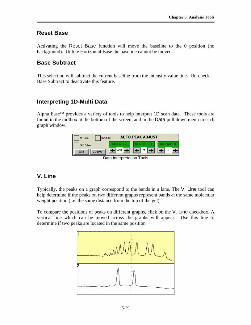
Chapter 5: Analysis Tools
5-29
Reset Base Activating the Reset Base function will move the baseline to the 0 position (no background). Unlike Horizontal Base the baseline cannot be moved.
Base Subtract This selection will subtract the current baseline from the intensity value line. Un-check Base Subtract to deactivate this feature. Interpreting 1D-Multi Data Alpha Ease™ provides a variety of tools to help interpret 1D scan data. These tools are found in the toolbox at the bottom of the screen, and in the Data pull down menu in each graph window.
Data Interpretation Tools
V. Line Typically, the peaks on a graph correspond to the bands in a lane. The V. Line tool can help determine if the peaks on two different graphs represent bands at the same molecular weight position (i.e. the same distance from the top of the gel). To compare the positions of peaks on different graphs, click on the V. Line checkbox. A vertical line which can be moved across the graphs will appear. Use this line to determine if two peaks are located in the same position
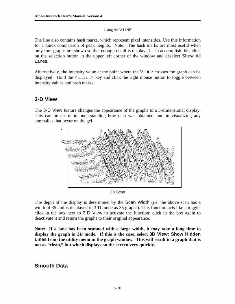
Alpha Innotech User’s Manual, version 4
5-30
Using the V.LINE The line also contains hash marks, which represent pixel intensities. Use this information for a quick comparison of peak heights. Note: The hash marks are most useful when only four graphs are shown so that enough detail is displayed. To accomplish this, click on the selection button in the upper left corner of the window and deselect Show All Lanes. Alternatively, the intensity value at the point where the V.Line crosses the graph can be displayed. Hold the <shift> key and click the right mouse button to toggle between intensity values and hash marks. 3-D View The 3-D View feature changes the appearance of the graphs to a 3-dimensional display. This can be useful in understanding how data was obtained, and in visualizing any anomalies that occur on the gel.
3D Scan
The depth of the display is determined by the Scan Width (i.e. the above scan has a width of 35 and is displayed in 3-D mode as 35 graphs). This function acts like a toggle: click in the box next to 3-D View to activate the function; click in the box again to deactivate it and return the graphs to their original appearance. Note: If a lane has been scanned with a large width, it may take a long time to display the graph in 3D mode. If this is the case, select 3D View: Show Hidden Lines from the utility menu in the graph window. This will result in a graph that is not as “clean,” but which displays on the screen very quickly.
Smooth Data
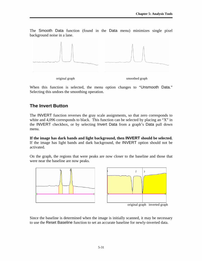
Chapter 5: Analysis Tools
5-31
The Smooth Data function (found in the Data menu) minimizes single pixel background noise in a lane.
original graph smoothed graph When this function is selected, the menu option changes to “Unsmooth Data.” Selecting this undoes the smoothing operation. The Invert Button The INVERT function reverses the gray scale assignments, so that zero corresponds to white and 4,096 corresponds to black. This function can be selected by placing an “X” in the INVERT checkbox, or by selecting Invert Data from a graph’s Data pull down menu. If the image has dark bands and light background, then INVERT should be selected. If the image has light bands and dark background, the INVERT option should not be activated. On the graph, the regions that were peaks are now closer to the baseline and those that were near the baseline are now peaks.
original graph inverted graph Since the baseline is determined when the image is initially scanned, it may be necessary to use the Reset Baseline function to set an accurate baseline for newly-inverted data.
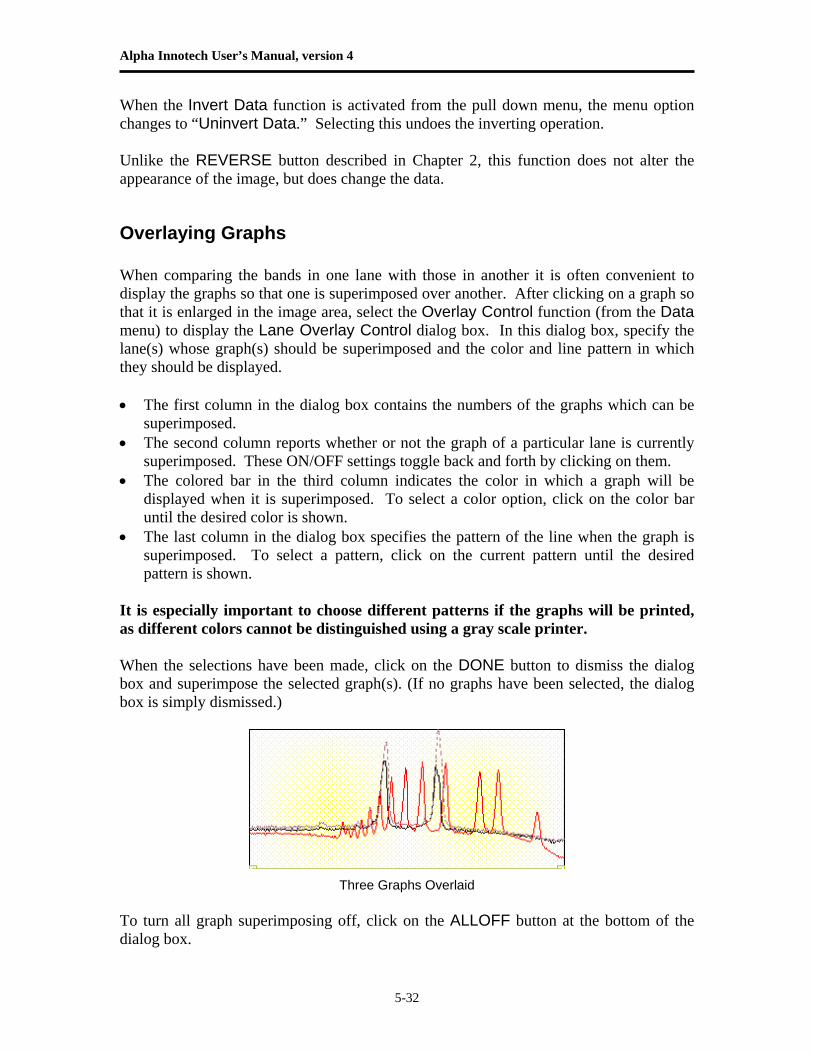
Alpha Innotech User’s Manual, version 4
5-32
When the Invert Data function is activated from the pull down menu, the menu option changes to “Uninvert Data.” Selecting this undoes the inverting operation. Unlike the REVERSE button described in Chapter 2, this function does not alter the appearance of the image, but does change the data.
Overlaying Graphs When comparing the bands in one lane with those in another it is often convenient to display the graphs so that one is superimposed over another. After clicking on a graph so that it is enlarged in the image area, select the Overlay Control function (from the Data menu) to display the Lane Overlay Control dialog box. In this dialog box, specify the lane(s) whose graph(s) should be superimposed and the color and line pattern in which they should be displayed. • The first column in the dialog box contains the numbers of the graphs which can be
superimposed. • The second column reports whether or not the graph of a particular lane is currently
superimposed. These ON/OFF settings toggle back and forth by clicking on them. • The colored bar in the third column indicates the color in which a graph will be
displayed when it is superimposed. To select a color option, click on the color bar until the desired color is shown.
• The last column in the dialog box specifies the pattern of the line when the graph is superimposed. To select a pattern, click on the current pattern until the desired pattern is shown.
It is especially important to choose different patterns if the graphs will be printed, as different colors cannot be distinguished using a gray scale printer. When the selections have been made, click on the DONE button to dismiss the dialog box and superimpose the selected graph(s). (If no graphs have been selected, the dialog box is simply dismissed.)
Three Graphs Overlaid
To turn all graph superimposing off, click on the ALLOFF button at the bottom of the dialog box.
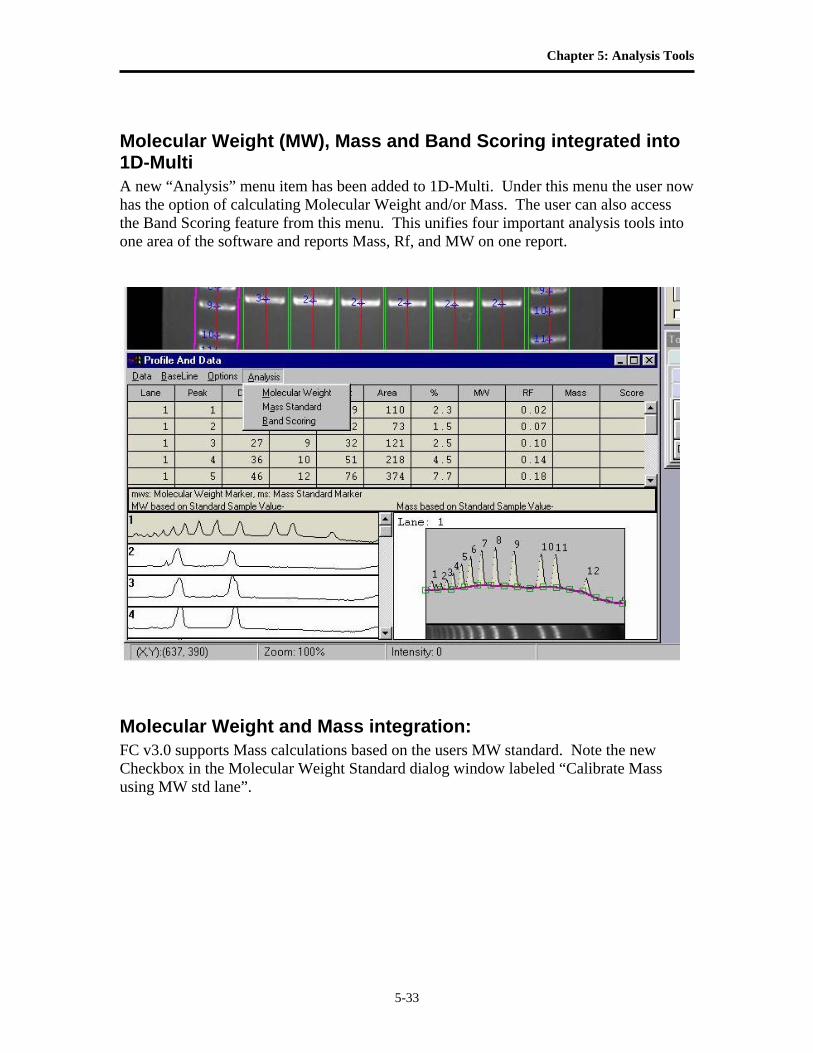
Chapter 5: Analysis Tools
5-33
Molecular Weight (MW), Mass and Band Scoring integrated into 1D-Multi A new “Analysis” menu item has been added to 1D-Multi. Under this menu the user now has the option of calculating Molecular Weight and/or Mass. The user can also access the Band Scoring feature from this menu. This unifies four important analysis tools into one area of the software and reports Mass, Rf, and MW on one report.
Molecular Weight and Mass integration: FC v3.0 supports Mass calculations based on the users MW standard. Note the new Checkbox in the Molecular Weight Standard dialog window labeled “Calibrate Mass using MW std lane”.
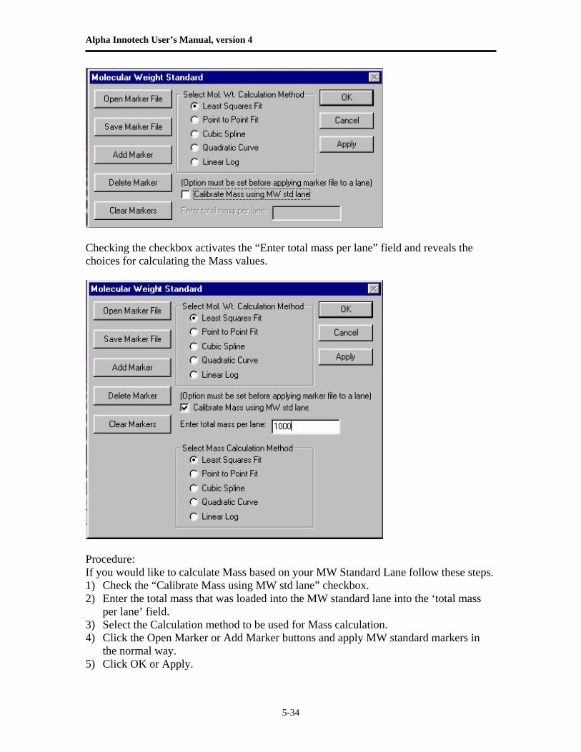
Alpha Innotech User’s Manual, version 4
5-34
Checking the checkbox activates the “Enter total mass per lane” field and reveals the choices for calculating the Mass values.
Procedure: If you would like to calculate Mass based on your MW Standard Lane follow these steps. 1) Check the “Calibrate Mass using MW std lane” checkbox. 2) Enter the total mass that was loaded into the MW standard lane into the ‘total mass
per lane’ field. 3) Select the Calculation method to be used for Mass calculation. 4) Click the Open Marker or Add Marker buttons and apply MW standard markers in
the normal way. 5) Click OK or Apply.
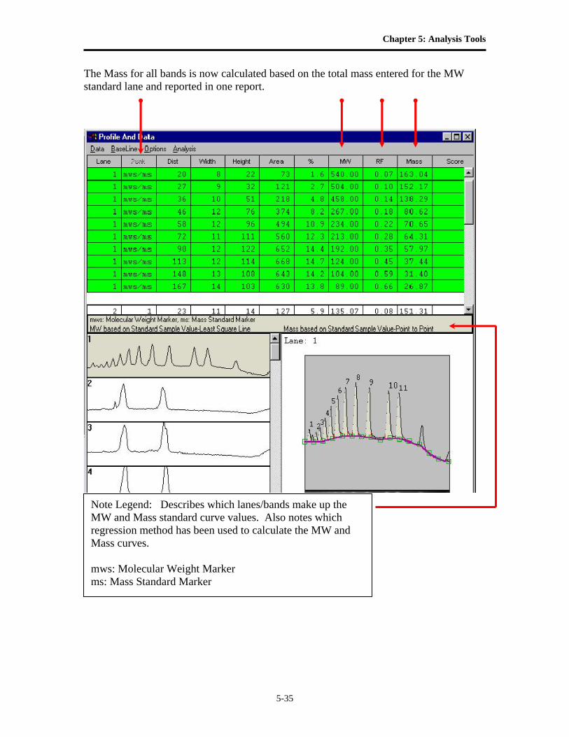
Chapter 5: Analysis Tools
5-35
The Mass for all bands is now calculated based on the total mass entered for the MW standard lane and reported in one report.
Note Legend: Describes which lanes/bands make up the MW and Mass standard curve values. Also notes which regression method has been used to calculate the MW and Mass curves. mws: Molecular Weight Marker ms: Mass Standard Marker
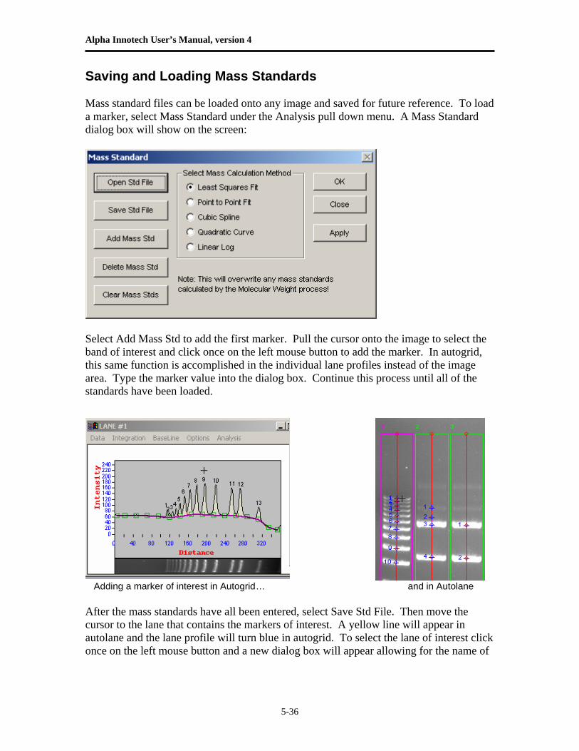
Alpha Innotech User’s Manual, version 4
5-36
Saving and Loading Mass Standards Mass standard files can be loaded onto any image and saved for future reference. To load a marker, select Mass Standard under the Analysis pull down menu. A Mass Standard dialog box will show on the screen:
Select Add Mass Std to add the first marker. Pull the cursor onto the image to select the band of interest and click once on the left mouse button to add the marker. In autogrid, this same function is accomplished in the individual lane profiles instead of the image area. Type the marker value into the dialog box. Continue this process until all of the standards have been loaded.
Adding a marker of interest in Autogrid … and in Autolane After the mass standards have all been entered, select Save Std File. Then move the cursor to the lane that contains the markers of interest. A yellow line will appear in autolane and the lane profile will turn blue in autogrid. To select the lane of interest click once on the left mouse button and a new dialog box will appear allowing for the name of
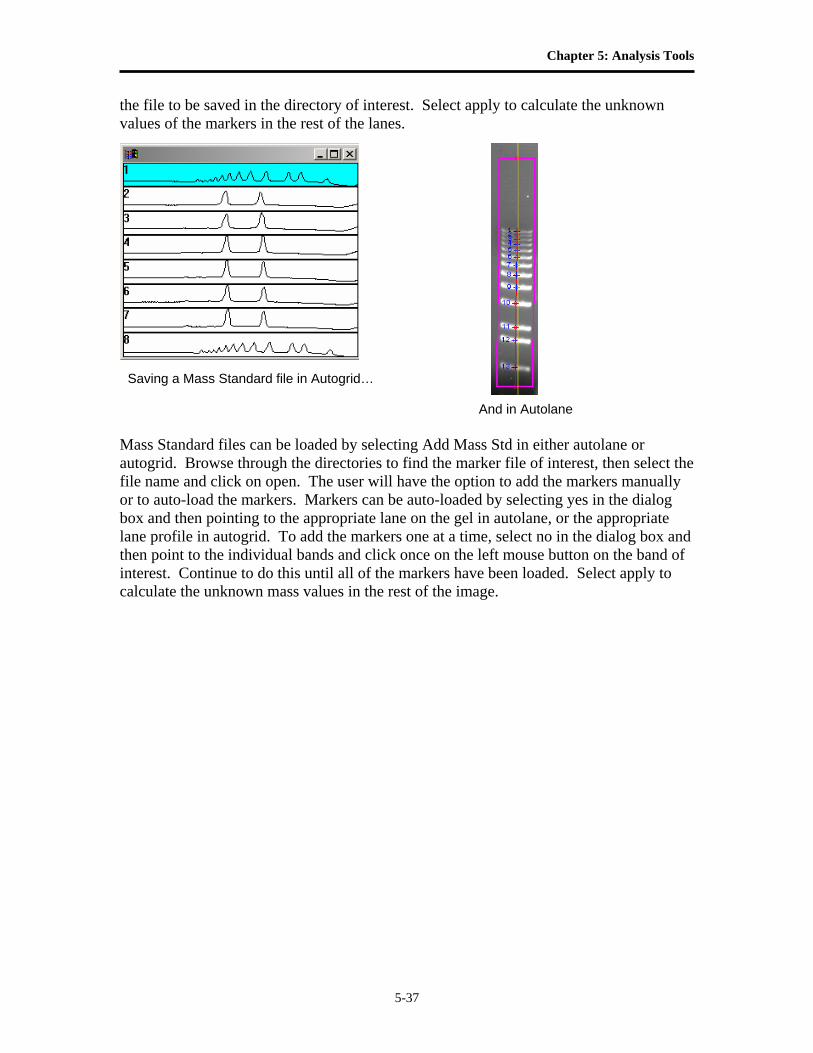
Chapter 5: Analysis Tools
5-37
the file to be saved in the directory of interest. Select apply to calculate the unknown values of the markers in the rest of the lanes.
Saving a Mass Standard file in Autogrid… And in Autolane Mass Standard files can be loaded by selecting Add Mass Std in either autolane or autogrid. Browse through the directories to find the marker file of interest, then select the file name and click on open. The user will have the option to add the markers manually or to auto-load the markers. Markers can be auto-loaded by selecting yes in the dialog box and then pointing to the appropriate lane on the gel in autolane, or the appropriate lane profile in autogrid. To add the markers one at a time, select no in the dialog box and then point to the individual bands and click once on the left mouse button on the band of interest. Continue to do this until all of the markers have been loaded. Select apply to calculate the unknown mass values in the rest of the image.
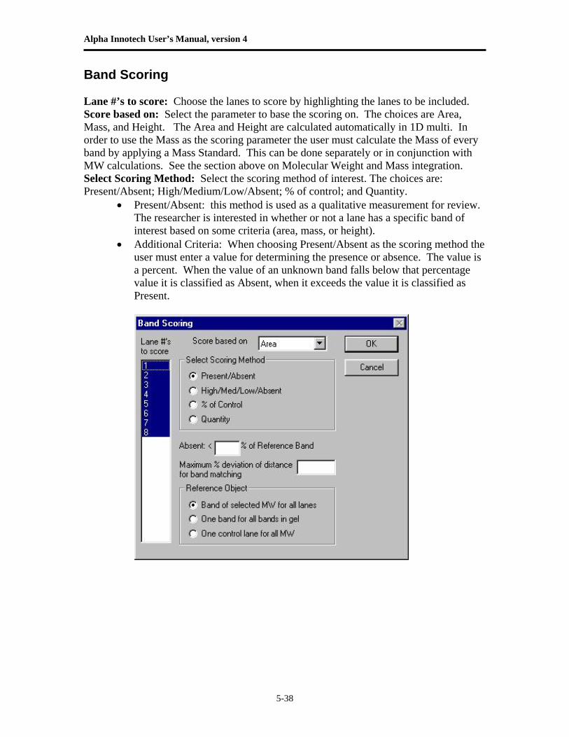
Alpha Innotech User’s Manual, version 4
5-38
Band Scoring Lane #’s to score: Choose the lanes to score by highlighting the lanes to be included. Score based on: Select the parameter to base the scoring on. The choices are Area, Mass, and Height. The Area and Height are calculated automatically in 1D multi. In order to use the Mass as the scoring parameter the user must calculate the Mass of every band by applying a Mass Standard. This can be done separately or in conjunction with MW calculations. See the section above on Molecular Weight and Mass integration. Select Scoring Method: Select the scoring method of interest. The choices are: Present/Absent; High/Medium/Low/Absent; % of control; and Quantity.
• Present/Absent: this method is used as a qualitative measurement for review. The researcher is interested in whether or not a lane has a specific band of interest based on some criteria (area, mass, or height).
• Additional Criteria: When choosing Present/Absent as the scoring method the user must enter a value for determining the presence or absence. The value is a percent. When the value of an unknown band falls below that percentage value it is classified as Absent, when it exceeds the value it is classified as Present.
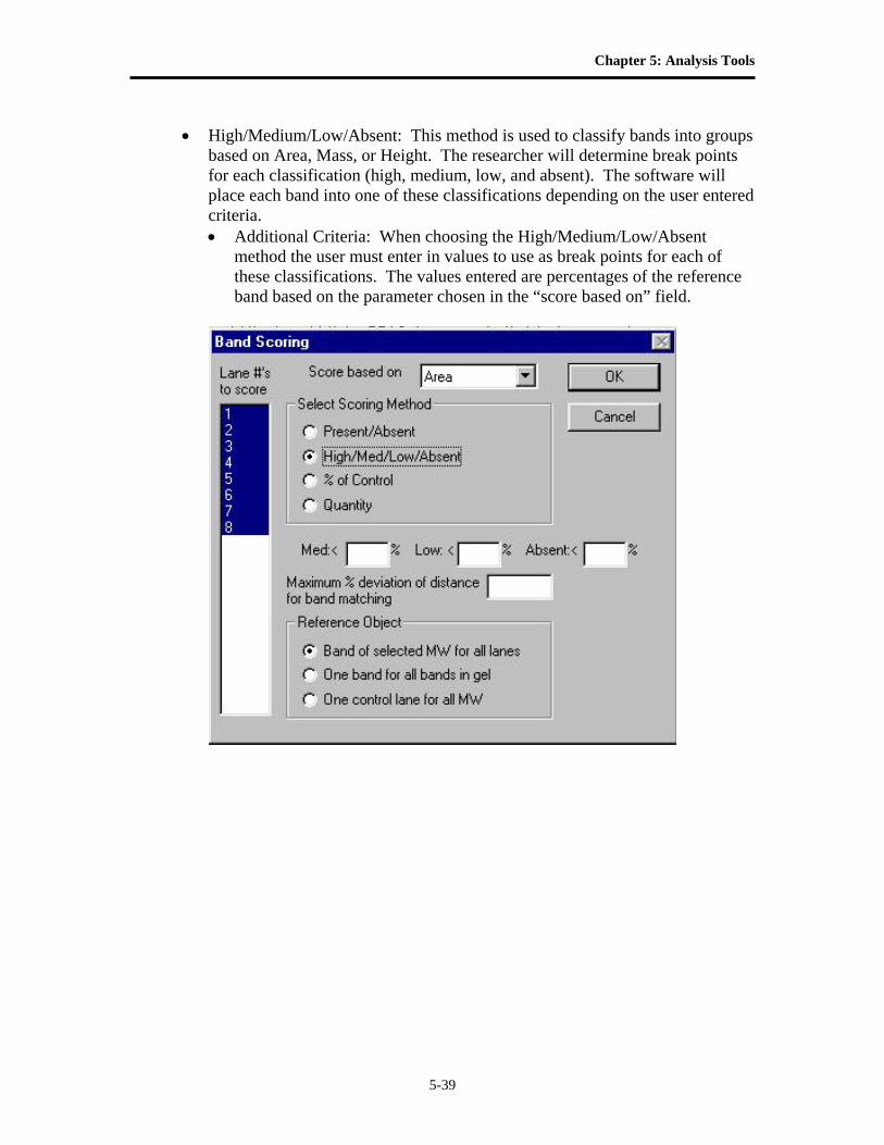
Chapter 5: Analysis Tools
5-39
• High/Medium/Low/Absent: This method is used to classify bands into groups
based on Area, Mass, or Height. The researcher will determine break points for each classification (high, medium, low, and absent). The software will place each band into one of these classifications depending on the user entered criteria. • Additional Criteria: When choosing the High/Medium/Low/Absent
method the user must enter in values to use as break points for each of these classifications. The values entered are percentages of the reference band based on the parameter chosen in the “score based on” field.
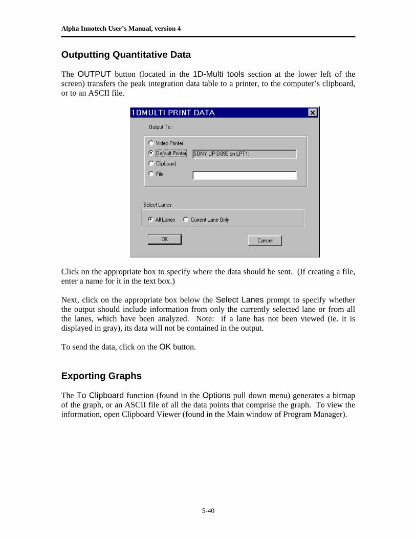
Alpha Innotech User’s Manual, version 4
5-40
Outputting Quantitative Data The OUTPUT button (located in the 1D-Multi tools section at the lower left of the screen) transfers the peak integration data table to a printer, to the computer’s clipboard, or to an ASCII file.
Click on the appropriate box to specify where the data should be sent. (If creating a file, enter a name for it in the text box.) Next, click on the appropriate box below the Select Lanes prompt to specify whether the output should include information from only the currently selected lane or from all the lanes, which have been analyzed. Note: if a lane has not been viewed (ie. it is displayed in gray), its data will not be contained in the output. To send the data, click on the OK button.
Exporting Graphs The To Clipboard function (found in the Options pull down menu) generates a bitmap of the graph, or an ASCII file of all the data points that comprise the graph. To view the information, open Clipboard Viewer (found in the Main window of Program Manager).
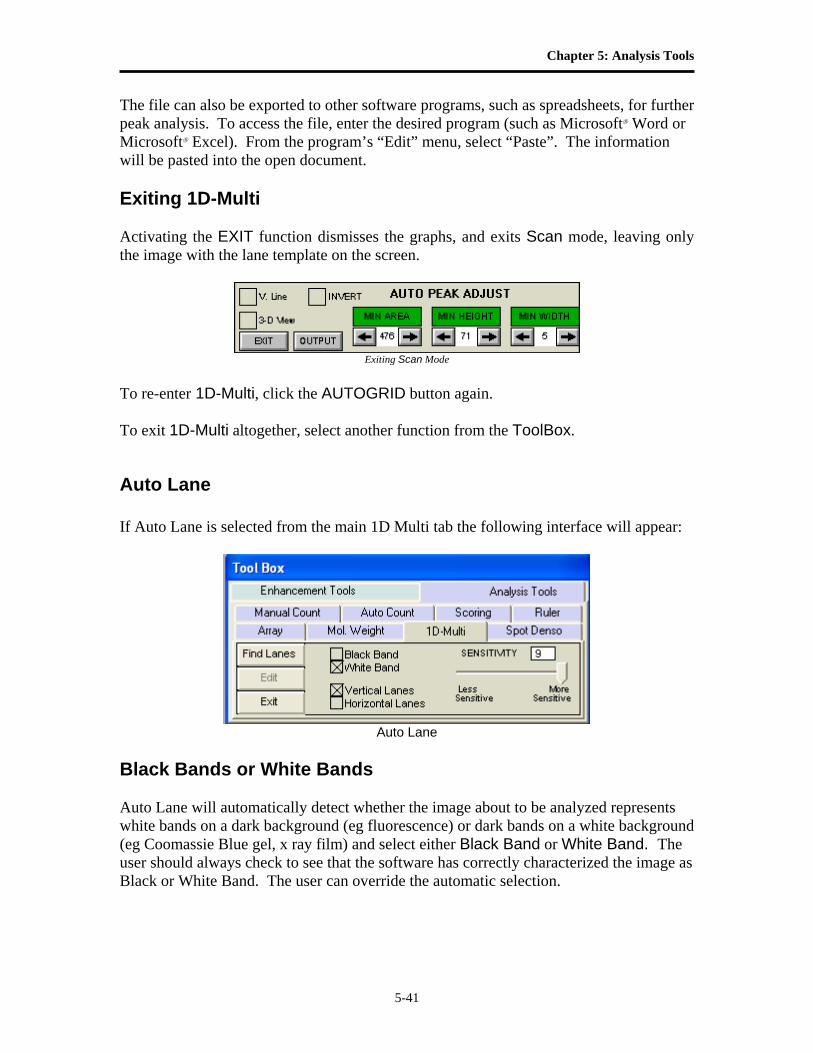
Chapter 5: Analysis Tools
5-41
The file can also be exported to other software programs, such as spreadsheets, for further peak analysis. To access the file, enter the desired program (such as Microsoft® Word or Microsoft® Excel). From the program’s “Edit” menu, select “Paste”. The information will be pasted into the open document. Exiting 1D-Multi Activating the EXIT function dismisses the graphs, and exits Scan mode, leaving only the image with the lane template on the screen.
Exiting Scan Mode
To re-enter 1D-Multi, click the AUTOGRID button again. To exit 1D-Multi altogether, select another function from the ToolBox.
Auto Lane
If Auto Lane is selected from the main 1D Multi tab the following interface will appear:
Auto Lane
Black Bands or White Bands Auto Lane will automatically detect whether the image about to be analyzed represents white bands on a dark background (eg fluorescence) or dark bands on a white background (eg Coomassie Blue gel, x ray film) and select either Black Band or White Band. The user should always check to see that the software has correctly characterized the image as Black or White Band. The user can override the automatic selection.
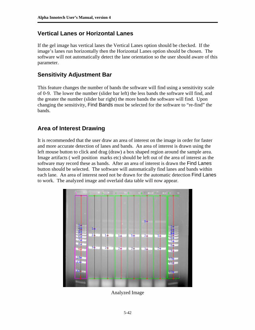
Alpha Innotech User’s Manual, version 4
5-42
Vertical Lanes or Horizontal Lanes If the gel image has vertical lanes the Vertical Lanes option should be checked. If the image’s lanes run horizontally then the Horizontal Lanes option should be chosen. The software will not automatically detect the lane orientation so the user should aware of this parameter. Sensitivity Adjustment Bar This feature changes the number of bands the software will find using a sensitivity scale of 0-9. The lower the number (slider bar left) the less bands the software will find, and the greater the number (slider bar right) the more bands the software will find. Upon changing the sensitivity, Find Bands must be selected for the software to “re-find” the bands. Area of Interest Drawing It is recommended that the user draw an area of interest on the image in order for faster and more accurate detection of lanes and bands. An area of interest is drawn using the left mouse button to click and drag (draw) a box shaped region around the sample area. Image artifacts ( well position marks etc) should be left out of the area of interest as the software may record these as bands. After an area of interest is drawn the Find Lanes button should be selected. The software will automatically find lanes and bands within each lane. An area of interest need not be drawn for the automatic detection Find Lanes to work. The analyzed image and overlaid data table will now appear.
Analyzed Image
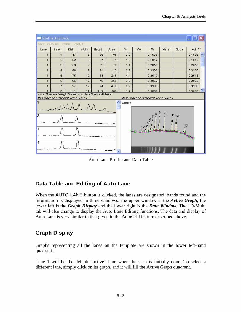
Chapter 5: Analysis Tools
5-43
Auto Lane Profile and Data Table
Data Table and Editing of Auto Lane When the AUTO LANE button is clicked, the lanes are designated, bands found and the information is displayed in three windows: the upper window is the Active Graph, the lower left is the Graph Display and the lower right is the Data Window. The 1D-Multi tab will also change to display the Auto Lane Editing functions. The data and display of Auto Lane is very similar to that given in the AutoGrid feature described above.
Graph Display Graphs representing all the lanes on the template are shown in the lower left-hand quadrant. Lane 1 will be the default “active” lane when the scan is initially done. To select a different lane, simply click on its graph, and it will fill the Active Graph quadrant.
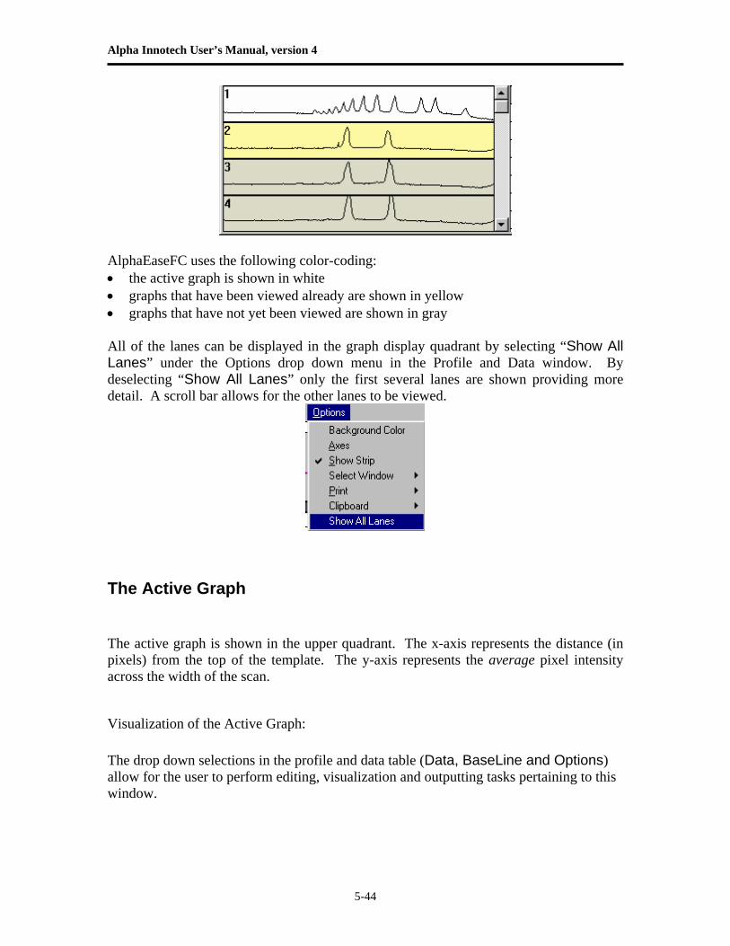
Alpha Innotech User’s Manual, version 4
5-44
AlphaEaseFC uses the following color-coding: • the active graph is shown in white • graphs that have been viewed already are shown in yellow • graphs that have not yet been viewed are shown in gray All of the lanes can be displayed in the graph display quadrant by selecting “Show All Lanes” under the Options drop down menu in the Profile and Data window. By deselecting “Show All Lanes” only the first several lanes are shown providing more detail. A scroll bar allows for the other lanes to be viewed.
The Active Graph
The active graph is shown in the upper quadrant. The x-axis represents the distance (in pixels) from the top of the template. The y-axis represents the average pixel intensity across the width of the scan.
Visualization of the Active Graph: The drop down selections in the profile and data table (Data, BaseLine and Options) allow for the user to perform editing, visualization and outputting tasks pertaining to this window.
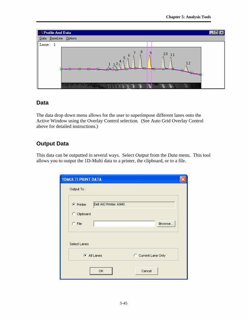
Chapter 5: Analysis Tools
5-45
Data The data drop down menu allows for the user to superimpose different lanes onto the Active Window using the Overlay Control selection. (See Auto Grid Overlay Control above for detailed instructions.) Output Data This data can be outputted in several ways. Select Output from the Data menu. This tool allows you to output the 1D-Multi data to a printer, the clipboard, or to a file.
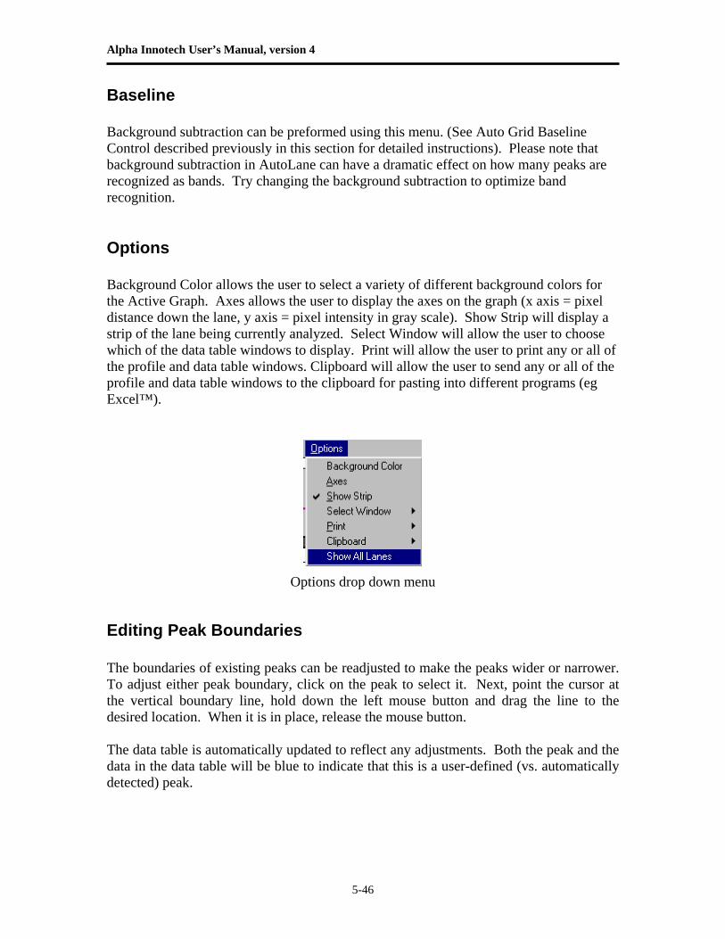
Alpha Innotech User’s Manual, version 4
5-46
Baseline Background subtraction can be preformed using this menu. (See Auto Grid Baseline Control described previously in this section for detailed instructions). Please note that background subtraction in AutoLane can have a dramatic effect on how many peaks are recognized as bands. Try changing the background subtraction to optimize band recognition. Options Background Color allows the user to select a variety of different background colors for the Active Graph. Axes allows the user to display the axes on the graph (x axis = pixel distance down the lane, y axis = pixel intensity in gray scale). Show Strip will display a strip of the lane being currently analyzed. Select Window will allow the user to choose which of the data table windows to display. Print will allow the user to print any or all of the profile and data table windows. Clipboard will allow the user to send any or all of the profile and data table windows to the clipboard for pasting into different programs (eg Excel™).
Options drop down menu
Editing Peak Boundaries The boundaries of existing peaks can be readjusted to make the peaks wider or narrower. To adjust either peak boundary, click on the peak to select it. Next, point the cursor at the vertical boundary line, hold down the left mouse button and drag the line to the desired location. When it is in place, release the mouse button. The data table is automatically updated to reflect any adjustments. Both the peak and the data in the data table will be blue to indicate that this is a user-defined (vs. automatically detected) peak.
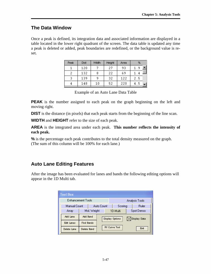
Chapter 5: Analysis Tools
5-47
The Data Window Once a peak is defined, its integration data and associated information are displayed in a table located in the lower right quadrant of the screen. The data table is updated any time a peak is deleted or added, peak boundaries are redefined, or the background value is re-set.
Example of an Auto Lane Data Table
PEAK is the number assigned to each peak on the graph beginning on the left and moving right.
DIST is the distance (in pixels) that each peak starts from the beginning of the line scan.
WIDTH and HEIGHT refer to the size of each peak.
AREA is the integrated area under each peak. This number reflects the intensity of each peak.
% is the percentage each peak contributes to the total density measured on the graph. (The sum of this column will be 100% for each lane.) Auto Lane Editing Features After the image has been evaluated for lanes and bands the following editing options will appear in the 1D Multi tab.
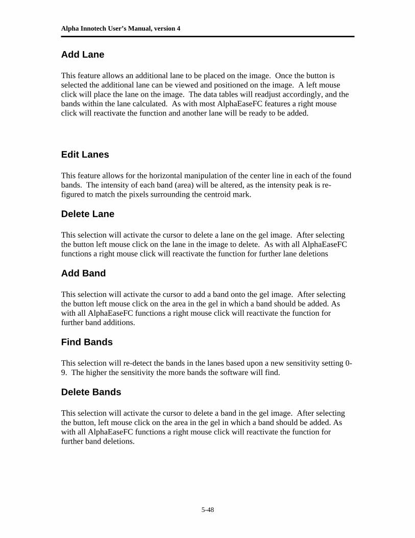
Alpha Innotech User’s Manual, version 4
5-48
Add Lane This feature allows an additional lane to be placed on the image. Once the button is selected the additional lane can be viewed and positioned on the image. A left mouse click will place the lane on the image. The data tables will readjust accordingly, and the bands within the lane calculated. As with most AlphaEaseFC features a right mouse click will reactivate the function and another lane will be ready to be added. Edit Lanes This feature allows for the horizontal manipulation of the center line in each of the found bands. The intensity of each band (area) will be altered, as the intensity peak is re-figured to match the pixels surrounding the centroid mark. Delete Lane This selection will activate the cursor to delete a lane on the gel image. After selecting the button left mouse click on the lane in the image to delete. As with all AlphaEaseFC functions a right mouse click will reactivate the function for further lane deletions Add Band This selection will activate the cursor to add a band onto the gel image. After selecting the button left mouse click on the area in the gel in which a band should be added. As with all AlphaEaseFC functions a right mouse click will reactivate the function for further band additions. Find Bands This selection will re-detect the bands in the lanes based upon a new sensitivity setting 0-9. The higher the sensitivity the more bands the software will find. Delete Bands This selection will activate the cursor to delete a band in the gel image. After selecting the button, left mouse click on the area in the gel in which a band should be added. As with all AlphaEaseFC functions a right mouse click will reactivate the function for further band deletions.
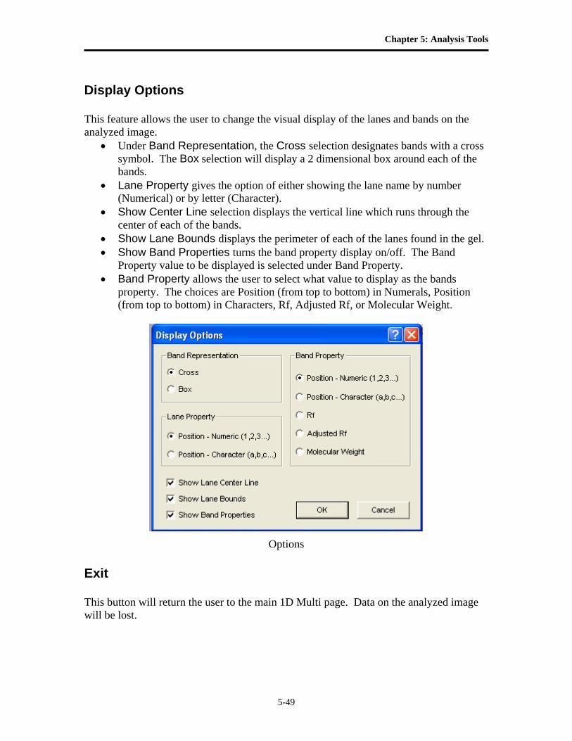
Chapter 5: Analysis Tools
5-49
Display Options This feature allows the user to change the visual display of the lanes and bands on the analyzed image.
• Under Band Representation, the Cross selection designates bands with a cross symbol. The Box selection will display a 2 dimensional box around each of the bands.
• Lane Property gives the option of either showing the lane name by number (Numerical) or by letter (Character).
• Show Center Line selection displays the vertical line which runs through the center of each of the bands.
• Show Lane Bounds displays the perimeter of each of the lanes found in the gel. • Show Band Properties turns the band property display on/off. The Band
Property value to be displayed is selected under Band Property. • Band Property allows the user to select what value to display as the bands
property. The choices are Position (from top to bottom) in Numerals, Position (from top to bottom) in Characters, Rf, Adjusted Rf, or Molecular Weight.
Options
Exit This button will return the user to the main 1D Multi page. Data on the analyzed image will be lost.
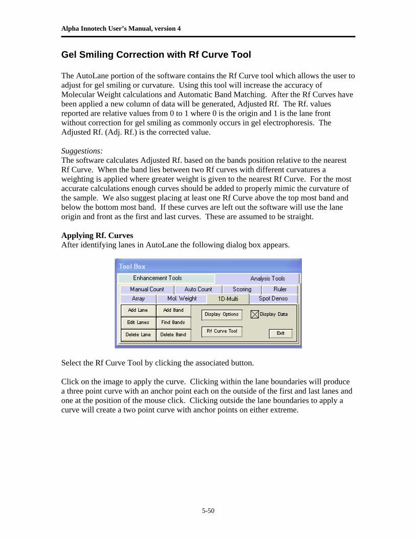
Alpha Innotech User’s Manual, version 4
5-50
Gel Smiling Correction with Rf Curve Tool The AutoLane portion of the software contains the Rf Curve tool which allows the user to adjust for gel smiling or curvature. Using this tool will increase the accuracy of Molecular Weight calculations and Automatic Band Matching. After the Rf Curves have been applied a new column of data will be generated, Adjusted Rf. The Rf. values reported are relative values from 0 to 1 where 0 is the origin and 1 is the lane front without correction for gel smiling as commonly occurs in gel electrophoresis. The Adjusted Rf. (Adj. Rf.) is the corrected value. Suggestions: The software calculates Adjusted Rf. based on the bands position relative to the nearest Rf Curve. When the band lies between two Rf curves with different curvatures a weighting is applied where greater weight is given to the nearest Rf Curve. For the most accurate calculations enough curves should be added to properly mimic the curvature of the sample. We also suggest placing at least one Rf Curve above the top most band and below the bottom most band. If these curves are left out the software will use the lane origin and front as the first and last curves. These are assumed to be straight. Applying Rf. Curves After identifying lanes in AutoLane the following dialog box appears.
Select the Rf Curve Tool by clicking the associated button. Click on the image to apply the curve. Clicking within the lane boundaries will produce a three point curve with an anchor point each on the outside of the first and last lanes and one at the position of the mouse click. Clicking outside the lane boundaries to apply a curve will create a two point curve with anchor points on either extreme.
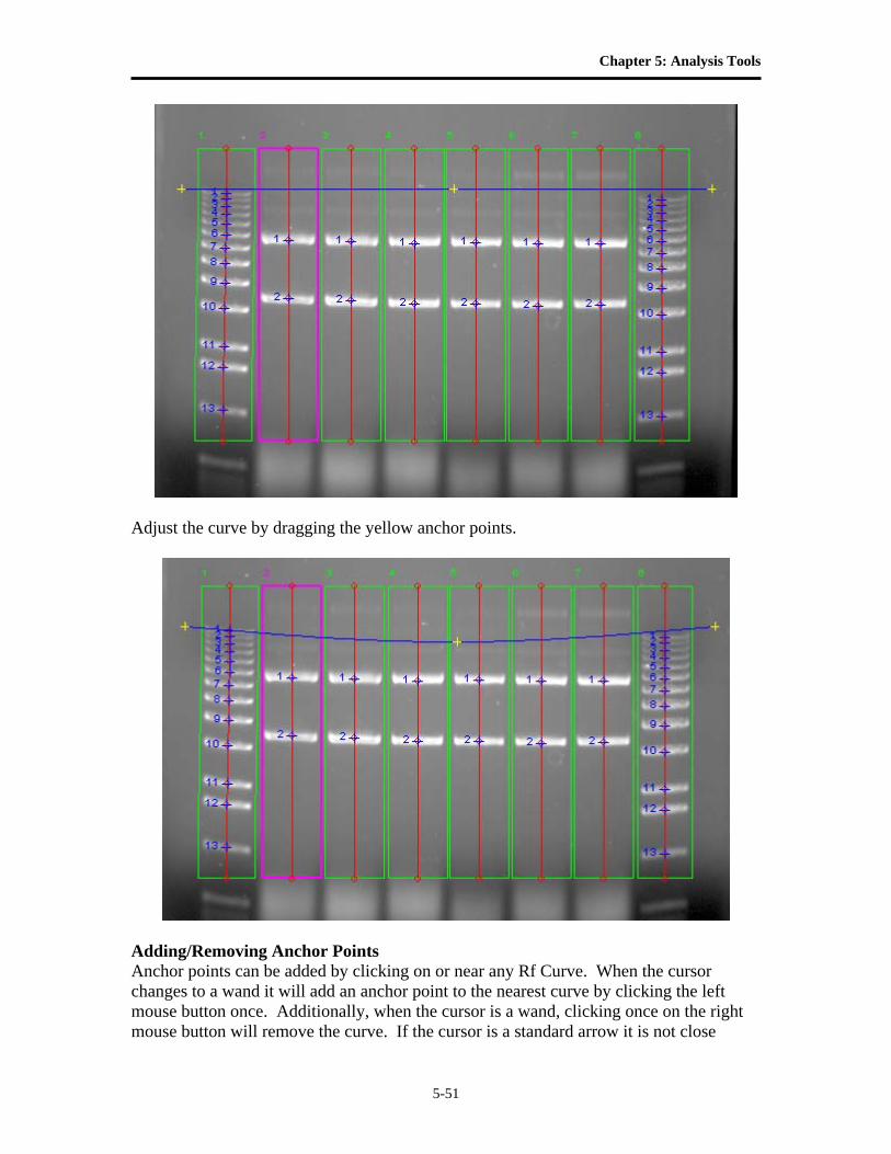
Chapter 5: Analysis Tools
5-51
Adjust the curve by dragging the yellow anchor points.
Adding/Removing Anchor Points Anchor points can be added by clicking on or near any Rf Curve. When the cursor changes to a wand it will add an anchor point to the nearest curve by clicking the left mouse button once. Additionally, when the cursor is a wand, clicking once on the right mouse button will remove the curve. If the cursor is a standard arrow it is not close
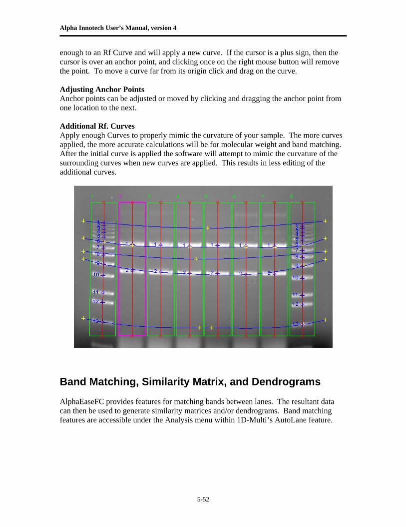
Alpha Innotech User’s Manual, version 4
5-52
enough to an Rf Curve and will apply a new curve. If the cursor is a plus sign, then the cursor is over an anchor point, and clicking once on the right mouse button will remove the point. To move a curve far from its origin click and drag on the curve. Adjusting Anchor Points Anchor points can be adjusted or moved by clicking and dragging the anchor point from one location to the next. Additional Rf. Curves Apply enough Curves to properly mimic the curvature of your sample. The more curves applied, the more accurate calculations will be for molecular weight and band matching. After the initial curve is applied the software will attempt to mimic the curvature of the surrounding curves when new curves are applied. This results in less editing of the additional curves.
Band Matching, Similarity Matrix, and Dendrograms AlphaEaseFC provides features for matching bands between lanes. The resultant data can then be used to generate similarity matrices and/or dendrograms. Band matching features are accessible under the Analysis menu within 1D-Multi’s AutoLane feature.
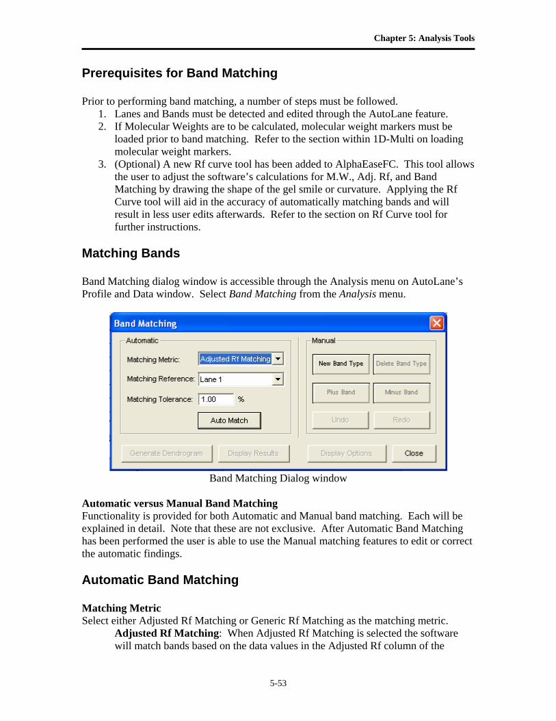
Chapter 5: Analysis Tools
5-53
Prerequisites for Band Matching Prior to performing band matching, a number of steps must be followed.
1. Lanes and Bands must be detected and edited through the AutoLane feature. 2. If Molecular Weights are to be calculated, molecular weight markers must be
loaded prior to band matching. Refer to the section within 1D-Multi on loading molecular weight markers.
3. (Optional) A new Rf curve tool has been added to AlphaEaseFC. This tool allows the user to adjust the software’s calculations for M.W., Adj. Rf, and Band Matching by drawing the shape of the gel smile or curvature. Applying the Rf Curve tool will aid in the accuracy of automatically matching bands and will result in less user edits afterwards. Refer to the section on Rf Curve tool for further instructions.
Matching Bands Band Matching dialog window is accessible through the Analysis menu on AutoLane’s Profile and Data window. Select Band Matching from the Analysis menu.
Band Matching Dialog window
Automatic versus Manual Band Matching Functionality is provided for both Automatic and Manual band matching. Each will be explained in detail. Note that these are not exclusive. After Automatic Band Matching has been performed the user is able to use the Manual matching features to edit or correct the automatic findings. Automatic Band Matching Matching Metric Select either Adjusted Rf Matching or Generic Rf Matching as the matching metric.
Adjusted Rf Matching: When Adjusted Rf Matching is selected the software will match bands based on the data values in the Adjusted Rf column of the
Alpha Innotech User’s Manual, version 4
5-54
Profile and Data window. These values result from the gel smile/curvature rather than the absolute vertical Rf value. Adjusted Rf is calculated based on the addition of M.W. markers and/or the Rf Curve lines which serve to correct the Generic Rf values for gel smiling. Generic Rf Matching: When Generic Rf Matching is selected the software will match bands based on the data values in the Rf column of the Profile and Data window. These values are the relative Rf calculated vertically where the origin of the lane is set to zero and the lane front is set to 1. Gel smiling or curvature is not adjusted for in this selection.
Matching Reference Select a lane to serve as the matching reference. It is advised that you choose a lane that either contains most of the bands of interest or spans the range of bands of interest while also containing many of the bands of interest. This will reduce the amount of effort required for post match edits. Matching Tolerance Enter a value to be used as the matching tolerance. The tolerance is converted into the amount of displacement two bands may have and still be matched by the software. The larger the tolerance value the larger the range the software will use for matching. The valid range is 0-10%. A value of 1-5% typically works best. A lower percentage works well for tightly spaced bands. Auto Match After selecting a matching metric, reference, and tolerance click the Auto Match button for the software to perform auto matching. When matching has been completed the Display Results and Generate Dendrogram buttons will become active. Refer to the appropriate sections below for a description of Similarity Results and Dendrogram creation. Editing Match Results Following Automatic band matching the user may need to manually edit or correct some matches. The tools under Manual Matching can be used for this purpose. Refer to the section below on Manual Matching for a description of each tool.
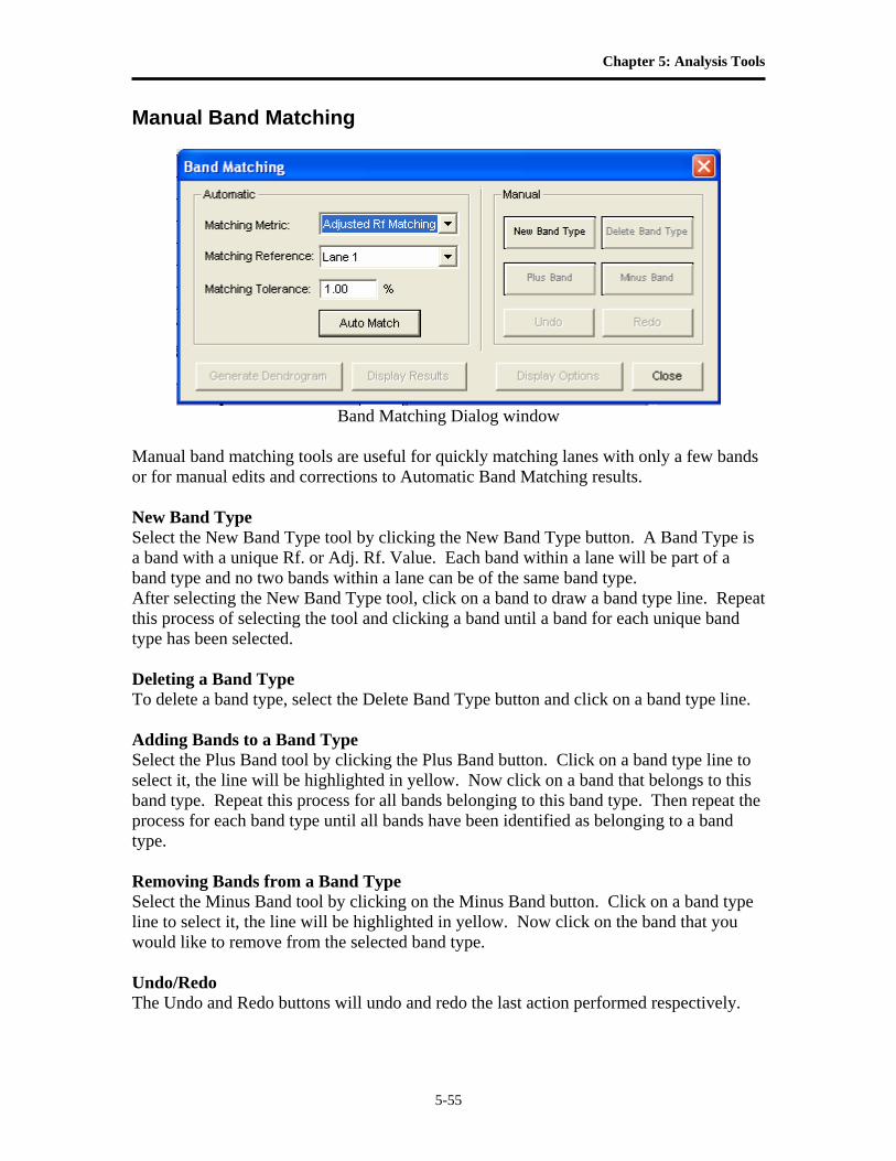
Chapter 5: Analysis Tools
5-55
Manual Band Matching
Band Matching Dialog window
Manual band matching tools are useful for quickly matching lanes with only a few bands or for manual edits and corrections to Automatic Band Matching results. New Band Type Select the New Band Type tool by clicking the New Band Type button. A Band Type is a band with a unique Rf. or Adj. Rf. Value. Each band within a lane will be part of a band type and no two bands within a lane can be of the same band type. After selecting the New Band Type tool, click on a band to draw a band type line. Repeat this process of selecting the tool and clicking a band until a band for each unique band type has been selected. Deleting a Band Type To delete a band type, select the Delete Band Type button and click on a band type line. Adding Bands to a Band Type Select the Plus Band tool by clicking the Plus Band button. Click on a band type line to select it, the line will be highlighted in yellow. Now click on a band that belongs to this band type. Repeat this process for all bands belonging to this band type. Then repeat the process for each band type until all bands have been identified as belonging to a band type. Removing Bands from a Band Type Select the Minus Band tool by clicking on the Minus Band button. Click on a band type line to select it, the line will be highlighted in yellow. Now click on the band that you would like to remove from the selected band type. Undo/Redo The Undo and Redo buttons will undo and redo the last action performed respectively.
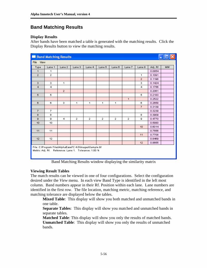
Alpha Innotech User’s Manual, version 4
5-56
Band Matching Results Display Results After bands have been matched a table is generated with the matching results. Click the Display Results button to view the matching results.
Band Matching Results window displaying the similarity matrix
Viewing Result Tables The match results can be viewed in one of four configurations. Select the configuration desired under the View menu. In each view Band Type is identified in the left most column. Band numbers appear in their Rf. Position within each lane. Lane numbers are identified in the first row. The file location, matching metric, matching reference, and matching tolerance are displayed below the tables.
Mixed Table: This display will show you both matched and unmatched bands in one table. Separate Tables: This display will show you matched and unmatched bands in separate tables. Matched Table: This display will show you only the results of matched bands. Unmatched Table: This display will show you only the results of unmatched bands.
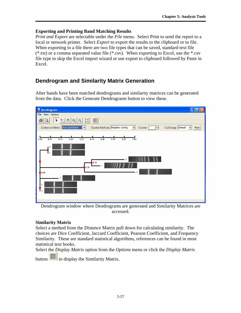
Chapter 5: Analysis Tools
5-57
Exporting and Printing Band Matching Results Print and Export are selectable under the File menu. Select Print to send the report to a local or network printer. Select Export to export the results to the clipboard or to file. When exporting to a file there are two file types that can be saved, standard text file (*.txt) or a comma separated value file (*.csv). When exporting to Excel, use the *.csv file type to skip the Excel import wizard or use export to clipboard followed by Paste in Excel. Dendrogram and Similarity Matrix Generation After bands have been matched dendrograms and similarity matrices can be generated from the data. Click the Generate Dendrograms button to view these.
Dendrogram window where Dendrograms are generated and Similarity Matrices are
accessed. Similarity Matrix Select a method from the Distance Matrix pull down for calculating similarity. The choices are Dice Coefficient, Jaccard Coefficient, Pearson Coefficient, and Frequency Similarity. These are standard statistical algorithms, references can be found in most statistical text books. Select the Display Matrix option from the Options menu or click the Display Matrix
button to display the Similarity Matrix.
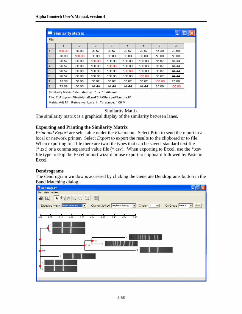
Alpha Innotech User’s Manual, version 4
5-58
Similarity Matrix
The similarity matrix is a graphical display of the similarity between lanes. Exporting and Printing the Similarity Matrix Print and Export are selectable under the File menu. Select Print to send the report to a local or network printer. Select Export to export the results to the clipboard or to file. When exporting to a file there are two file types that can be saved, standard text file (*.txt) or a comma separated value file (*.csv). When exporting to Excel, use the *.csv file type to skip the Excel import wizard or use export to clipboard followed by Paste in Excel. Dendrograms The dendrogram window is accessed by clicking the Generate Dendrograms button in the Band Matching dialog.
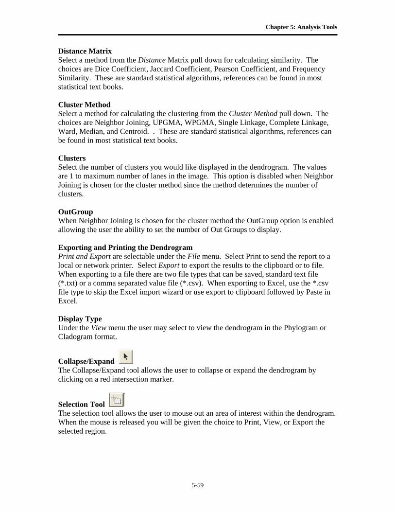
Chapter 5: Analysis Tools
5-59
Distance Matrix Select a method from the Distance Matrix pull down for calculating similarity. The choices are Dice Coefficient, Jaccard Coefficient, Pearson Coefficient, and Frequency Similarity. These are standard statistical algorithms, references can be found in most statistical text books. Cluster Method Select a method for calculating the clustering from the Cluster Method pull down. The choices are Neighbor Joining, UPGMA, WPGMA, Single Linkage, Complete Linkage, Ward, Median, and Centroid. . These are standard statistical algorithms, references can be found in most statistical text books. Clusters Select the number of clusters you would like displayed in the dendrogram. The values are 1 to maximum number of lanes in the image. This option is disabled when Neighbor Joining is chosen for the cluster method since the method determines the number of clusters. OutGroup When Neighbor Joining is chosen for the cluster method the OutGroup option is enabled allowing the user the ability to set the number of Out Groups to display. Exporting and Printing the Dendrogram Print and Export are selectable under the File menu. Select Print to send the report to a local or network printer. Select Export to export the results to the clipboard or to file. When exporting to a file there are two file types that can be saved, standard text file (*.txt) or a comma separated value file (*.csv). When exporting to Excel, use the *.csv file type to skip the Excel import wizard or use export to clipboard followed by Paste in Excel. Display Type Under the View menu the user may select to view the dendrogram in the Phylogram or Cladogram format.
Collapse/Expand The Collapse/Expand tool allows the user to collapse or expand the dendrogram by clicking on a red intersection marker.
Selection Tool The selection tool allows the user to mouse out an area of interest within the dendrogram. When the mouse is released you will be given the choice to Print, View, or Export the selected region.
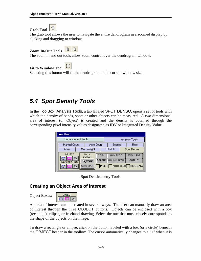
Alpha Innotech User’s Manual, version 4
5-60
Grab Tool The grab tool allows the user to navigate the entire dendrogram in a zoomed display by clicking and dragging to window.
Zoom In/Out Tools The zoom in and out tools allow zoom control over the dendrogram window.
Fit to Window Tool Selecting this button will fit the dendrogram to the current window size. 5.4 Spot Density Tools In the ToolBox, Analysis Tools, a tab labeled SPOT DENSO, opens a set of tools with which the density of bands, spots or other objects can be measured. A two dimensional area of interest (or Object) is created and the density is obtained through the corresponding pixel intensity values designated as IDV or Integrated Density Value.
Spot Densitometry Tools
Creating an Object Area of Interest Object Boxes: An area of interest can be created in several ways. The user can manually draw an area of interest through the three OBJECT buttons. Objects can be enclosed with a box (rectangle), ellipse, or freehand drawing. Select the one that most closely corresponds to the shape of the objects on the image. To draw a rectangle or ellipse, click on the button labeled with a box (or a circle) beneath the OBJECT header in the toolbox. The cursor automatically changes to a "+" when it is
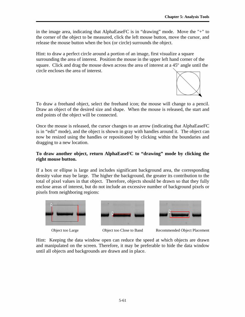
Chapter 5: Analysis Tools
5-61
in the image area, indicating that AlphaEaseFC is in “drawing” mode. Move the "+" to the corner of the object to be measured, click the left mouse button, move the cursor, and release the mouse button when the box (or circle) surrounds the object. Hint: to draw a perfect circle around a portion of an image, first visualize a square surrounding the area of interest. Position the mouse in the upper left hand corner of the square. Click and drag the mouse down across the area of interest at a 45° angle until the circle encloses the area of interest. To draw a freehand object, select the freehand icon; the mouse will change to a pencil. Draw an object of the desired size and shape. When the mouse is released, the start and end points of the object will be connected. Once the mouse is released, the cursor changes to an arrow (indicating that AlphaEaseFC is in “edit” mode), and the object is shown in gray with handles around it. The object can now be resized using the handles or repositioned by clicking within the boundaries and dragging to a new location. To draw another object, return AlphaEaseFC to “drawing” mode by clicking the right mouse button. If a box or ellipse is large and includes significant background area, the corresponding density value may be large. The higher the background, the greater its contribution to the total of pixel values in that object. Therefore, objects should be drawn so that they fully enclose areas of interest, but do not include an excessive number of background pixels or pixels from neighboring regions:
Object too Large Object too Close to Band Recommended Object Placement Hint: Keeping the data window open can reduce the speed at which objects are drawn and manipulated on the screen. Therefore, it may be preferable to hide the data window until all objects and backgrounds are drawn and in place.
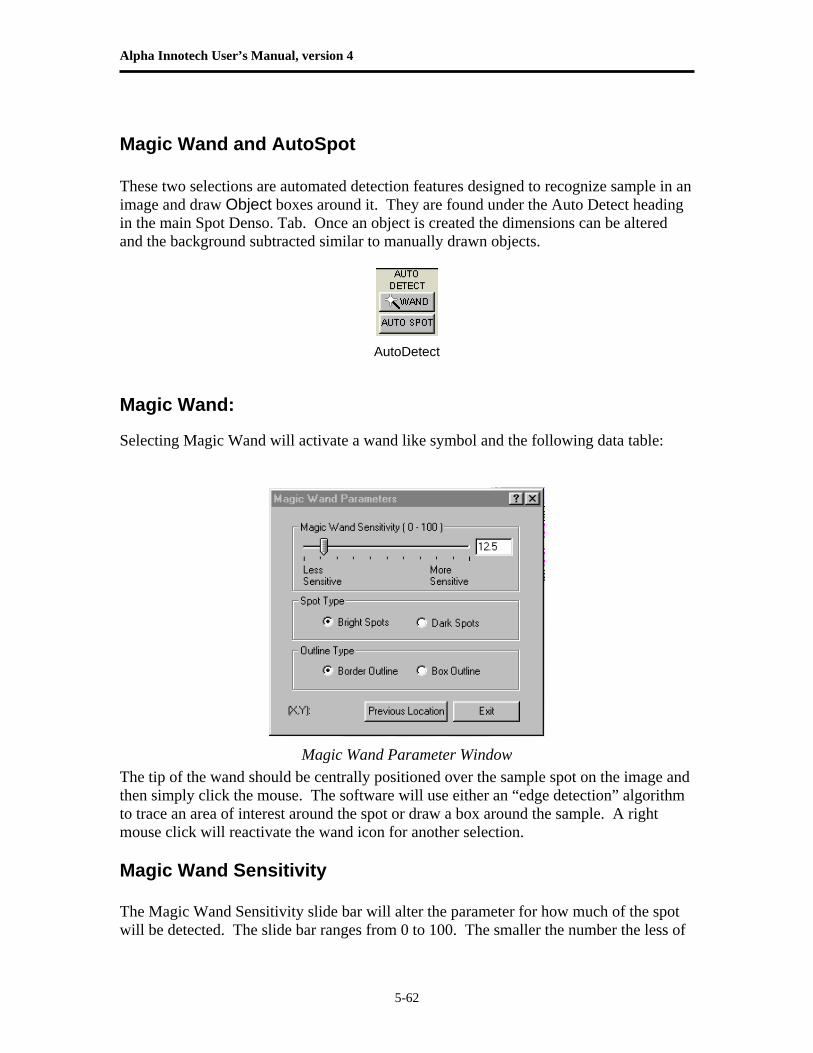
Alpha Innotech User’s Manual, version 4
5-62
Magic Wand and AutoSpot These two selections are automated detection features designed to recognize sample in an image and draw Object boxes around it. They are found under the Auto Detect heading in the main Spot Denso. Tab. Once an object is created the dimensions can be altered and the background subtracted similar to manually drawn objects.
AutoDetect
Magic Wand:
Selecting Magic Wand will activate a wand like symbol and the following data table:
Magic Wand Parameter Window
The tip of the wand should be centrally positioned over the sample spot on the image and then simply click the mouse. The software will use either an “edge detection” algorithm to trace an area of interest around the spot or draw a box around the sample. A right mouse click will reactivate the wand icon for another selection. Magic Wand Sensitivity The Magic Wand Sensitivity slide bar will alter the parameter for how much of the spot will be detected. The slide bar ranges from 0 to 100. The smaller the number the less of
Chapter 5: Analysis Tools
5-63
the spot the software will define. The greater the sensitivity number the more of the object the software will find. **HINT: Selecting a brighter pixel within the band (or spot) will have magic wand draw a tighter area of interest. Correspondingly, a less intense pixel will draw a larger perimeter around the selected spot** Spot Type Under the Spot Type heading the Bright Spots selection should be checked if the image contains bright spots on a dark background (e.g. ethidium bromide stained fluorescent gels and chemiluminescent blots). The Dark Spots selection should be made when the sample contains dark sample on a light background (film, coomassie blue protein gels etc..). The software should automatically determine this selection, but the user may have to override it if the software incorrectly evaluates an image. Remember as in all portions of AlphaEaseFC software if the image has been reversed (negative image)using the Reverse selection on the Contrast Adjustment window the Dark Spot selection should not be made. Reverse is a visual alteration only and does not effect the original image capture data. (EG a chemiluminescent blot is captured using the Reverse mode in order for it to appear as film, the correct selection is still Bright Spots). Outline Type Border Outline will use the edge detection methods to determine the spot area. The Box Outline will draw a box shape around the sample usually including a significant portion of background. User preference and image particulars will determine which outline type is best. Previous Location Previous Location will automatically select the spot on the image last selected for magic wand and apply any changes made for sensitivity. This feature is designed to quickly evaluate how the different sensitivity numbers will affect the drawn area using the same selected point in a spot. The X,Y coordinates are given for the previous spot as well. Exit Exit will remove the Magic Wand Parameter Window.
Auto Spot: Auto Spot is a feature designed to find multiple spots within a region of interest. It is accessed through AutoSpot under Auto Detect in the Spot Denso tab. Once it is selected the following tab will appear and the cursor will be ready to draw an area of interest.
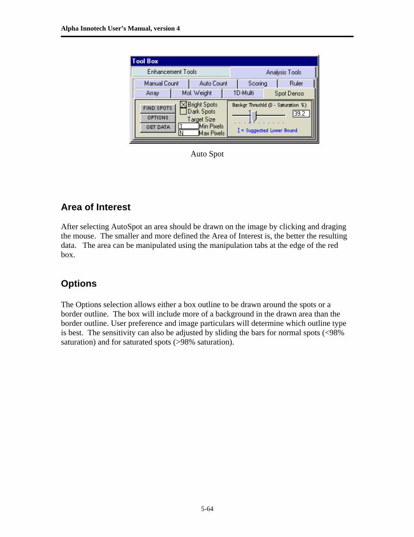
Alpha Innotech User’s Manual, version 4
5-64
Auto Spot
Area of Interest After selecting AutoSpot an area should be drawn on the image by clicking and draging the mouse. The smaller and more defined the Area of Interest is, the better the resulting data. The area can be manipulated using the manipulation tabs at the edge of the red box. Options The Options selection allows either a box outline to be drawn around the spots or a border outline. The box will include more of a background in the drawn area than the border outline. User preference and image particulars will determine which outline type is best. The sensitivity can also be adjusted by sliding the bars for normal spots (<98% saturation) and for saturated spots (>98% saturation).
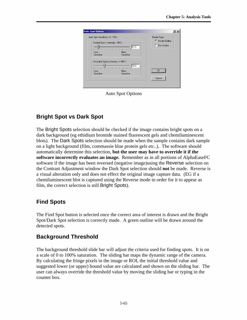
Chapter 5: Analysis Tools
5-65
Auto Spot Options
Bright Spot vs Dark Spot The Bright Spots selection should be checked if the image contains bright spots on a dark background (eg ethidium bromide stained fluorescent gels and chemiluminescent blots). The Dark Spots selection should be made when the sample contains dark sample on a light background (film, commassie blue protein gels etc..). The software should automatically determine this selection, but the user may have to override it if the software incorrectly evaluates an image. Remember as in all portions of AlphaEaseFC software if the image has been reversed (negative image)using the Reverse selection on the Contrast Adjustment window the Dark Spot selection should not be made. Reverse is a visual alteration only and does not effect the original image capture data. (EG if a chemiluminescent blot is captured using the Reverse mode in order for it to appear as film, the correct selection is still Bright Spots).
Find Spots The Find Spot button is selected once the correct area of interest is drawn and the Bright Spot/Dark Spot selection is correctly made. A green outline will be drawn around the detected spots.
Background Threshold The background threshold slide bar will adjust the criteria used for finding spots. It is on a scale of 0 to 100% saturation. The sliding bar maps the dynamic range of the camera. By calculating the fringe pixels in the image or ROI, the initial threshold value and suggested lower (or upper) bound value are calculated and shown on the sliding bar. The user can always override the threshold value by moving the sliding bar or typing in the counter box.
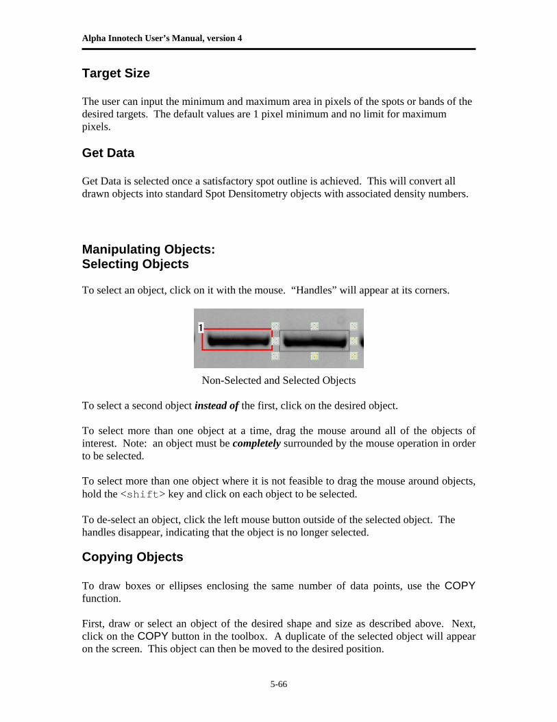
Alpha Innotech User’s Manual, version 4
5-66
Target Size The user can input the minimum and maximum area in pixels of the spots or bands of the desired targets. The default values are 1 pixel minimum and no limit for maximum pixels. Get Data Get Data is selected once a satisfactory spot outline is achieved. This will convert all drawn objects into standard Spot Densitometry objects with associated density numbers. Manipulating Objects: Selecting Objects To select an object, click on it with the mouse. “Handles” will appear at its corners.
Non-Selected and Selected Objects
To select a second object instead of the first, click on the desired object. To select more than one object at a time, drag the mouse around all of the objects of interest. Note: an object must be completely surrounded by the mouse operation in order to be selected. To select more than one object where it is not feasible to drag the mouse around objects, hold the <shift> key and click on each object to be selected. To de-select an object, click the left mouse button outside of the selected object. The handles disappear, indicating that the object is no longer selected.
Copying Objects To draw boxes or ellipses enclosing the same number of data points, use the COPY function. First, draw or select an object of the desired shape and size as described above. Next, click on the COPY button in the toolbox. A duplicate of the selected object will appear on the screen. This object can then be moved to the desired position.
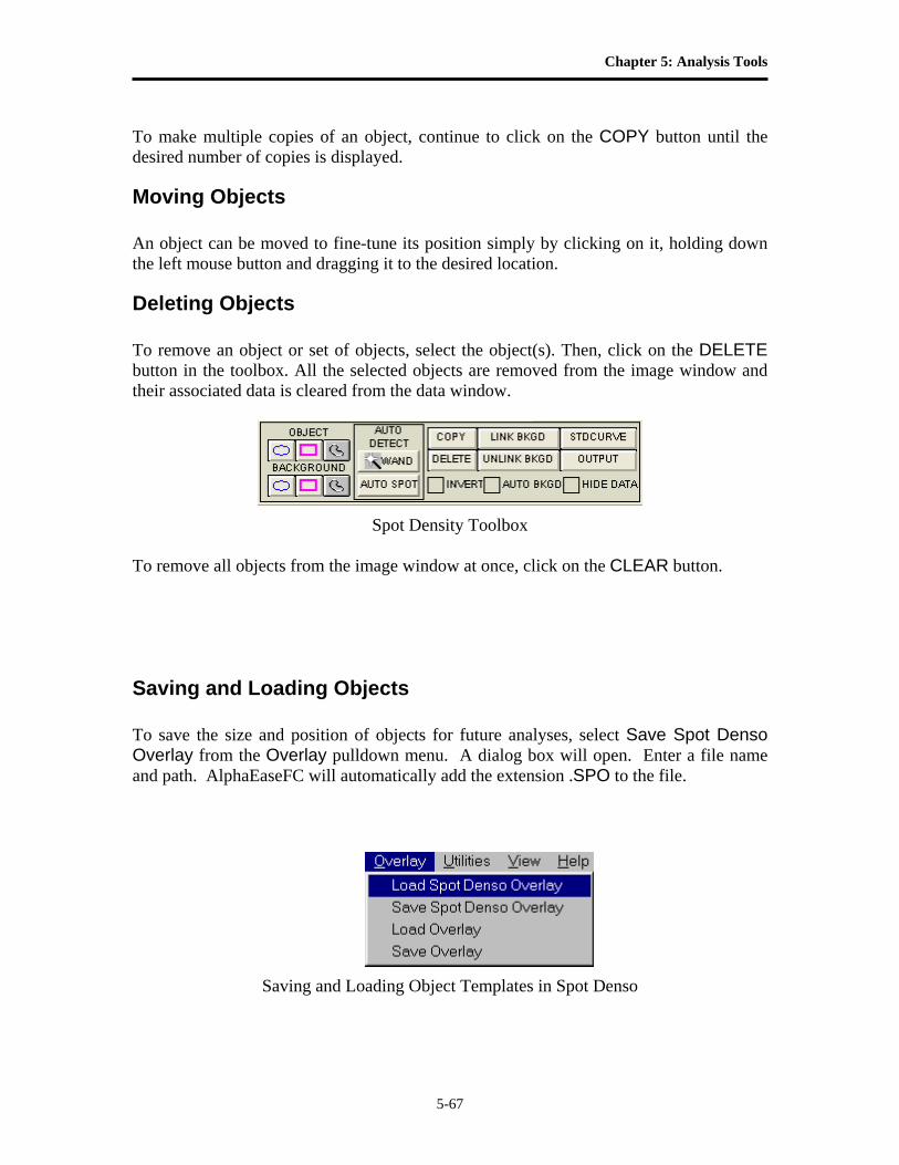
Chapter 5: Analysis Tools
5-67
To make multiple copies of an object, continue to click on the COPY button until the desired number of copies is displayed.
Moving Objects An object can be moved to fine-tune its position simply by clicking on it, holding down the left mouse button and dragging it to the desired location.
Deleting Objects To remove an object or set of objects, select the object(s). Then, click on the DELETE button in the toolbox. All the selected objects are removed from the image window and their associated data is cleared from the data window.
Spot Density Toolbox
To remove all objects from the image window at once, click on the CLEAR button.
Saving and Loading Objects To save the size and position of objects for future analyses, select Save Spot Denso Overlay from the Overlay pulldown menu. A dialog box will open. Enter a file name and path. AlphaEaseFC will automatically add the extension .SPO to the file.
Saving and Loading Object Templates in Spot Denso
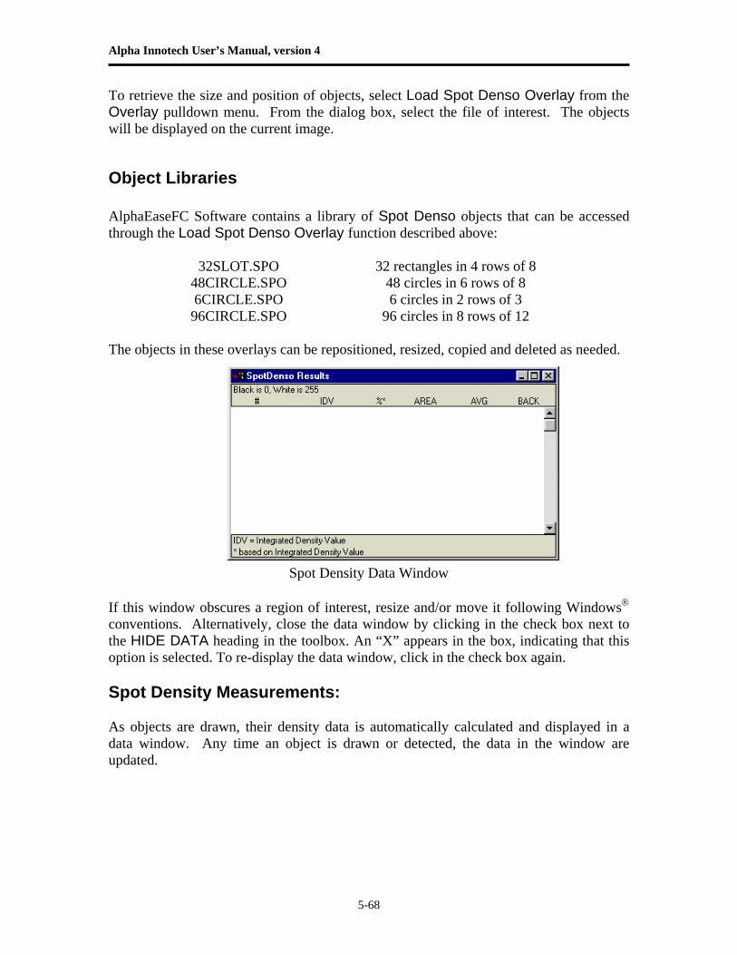
Alpha Innotech User’s Manual, version 4
5-68
To retrieve the size and position of objects, select Load Spot Denso Overlay from the Overlay pulldown menu. From the dialog box, select the file of interest. The objects will be displayed on the current image.
Object Libraries AlphaEaseFC Software contains a library of Spot Denso objects that can be accessed through the Load Spot Denso Overlay function described above: 32SLOT.SPO 32 rectangles in 4 rows of 8 48CIRCLE.SPO 48 circles in 6 rows of 8 6CIRCLE.SPO 6 circles in 2 rows of 3 96CIRCLE.SPO 96 circles in 8 rows of 12 The objects in these overlays can be repositioned, resized, copied and deleted as needed.
Spot Density Data Window If this window obscures a region of interest, resize and/or move it following Windows® conventions. Alternatively, close the data window by clicking in the check box next to the HIDE DATA heading in the toolbox. An “X” appears in the box, indicating that this option is selected. To re-display the data window, click in the check box again. Spot Density Measurements: As objects are drawn, their density data is automatically calculated and displayed in a data window. Any time an object is drawn or detected, the data in the window are updated.
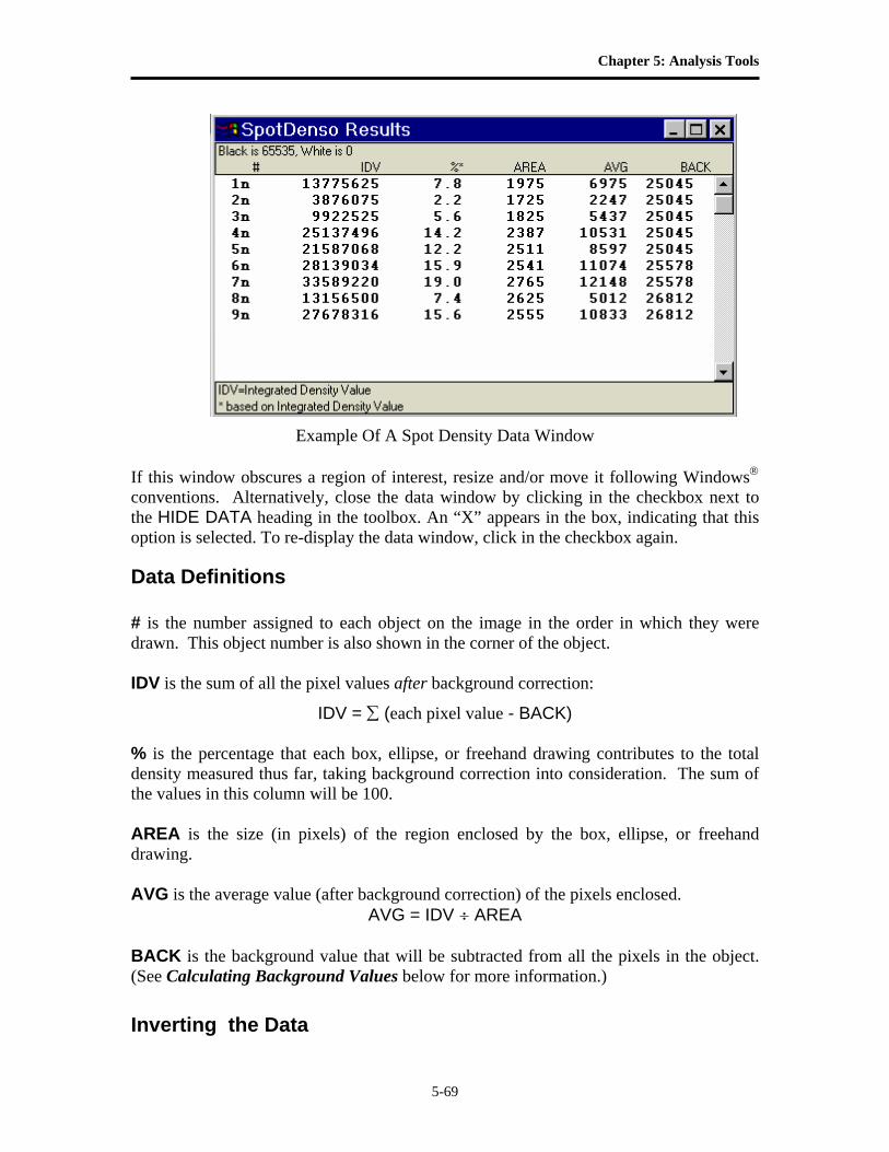
Chapter 5: Analysis Tools
5-69
Example Of A Spot Density Data Window If this window obscures a region of interest, resize and/or move it following Windows® conventions. Alternatively, close the data window by clicking in the checkbox next to the HIDE DATA heading in the toolbox. An “X” appears in the box, indicating that this option is selected. To re-display the data window, click in the checkbox again.
Data Definitions # is the number assigned to each object on the image in the order in which they were drawn. This object number is also shown in the corner of the object. IDV is the sum of all the pixel values after background correction:
IDV = ∑ (each pixel value - BACK) % is the percentage that each box, ellipse, or freehand drawing contributes to the total density measured thus far, taking background correction into consideration. The sum of the values in this column will be 100. AREA is the size (in pixels) of the region enclosed by the box, ellipse, or freehand drawing. AVG is the average value (after background correction) of the pixels enclosed.
AVG = IDV ÷ AREA BACK is the background value that will be subtracted from all the pixels in the object. (See Calculating Background Values below for more information.) Inverting the Data
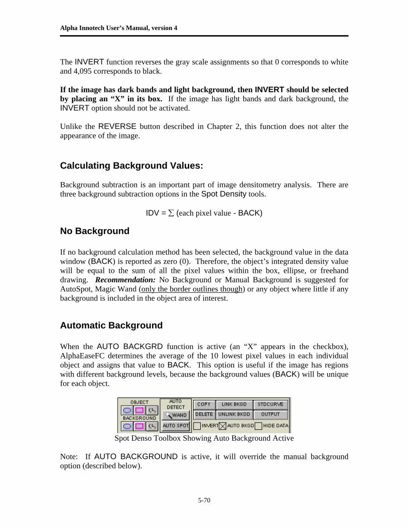
Alpha Innotech User’s Manual, version 4
5-70
The INVERT function reverses the gray scale assignments so that 0 corresponds to white and 4,095 corresponds to black. If the image has dark bands and light background, then INVERT should be selected by placing an “X” in its box. If the image has light bands and dark background, the INVERT option should not be activated. Unlike the REVERSE button described in Chapter 2, this function does not alter the appearance of the image. Calculating Background Values: Background subtraction is an important part of image densitometry analysis. There are three background subtraction options in the Spot Density tools.
IDV = ∑ (each pixel value - BACK)
No Background If no background calculation method has been selected, the background value in the data window (BACK) is reported as zero (0). Therefore, the object’s integrated density value will be equal to the sum of all the pixel values within the box, ellipse, or freehand drawing. Recommendation: No Background or Manual Background is suggested for AutoSpot, Magic Wand (only the border outlines though) or any object where little if any background is included in the object area of interest.
Automatic Background When the AUTO BACKGRD function is active (an “X” appears in the checkbox), AlphaEaseFC determines the average of the 10 lowest pixel values in each individual object and assigns that value to BACK. This option is useful if the image has regions with different background levels, because the background values (BACK) will be unique for each object.
Spot Denso Toolbox Showing Auto Background Active
Note: If AUTO BACKGROUND is active, it will override the manual background option (described below).
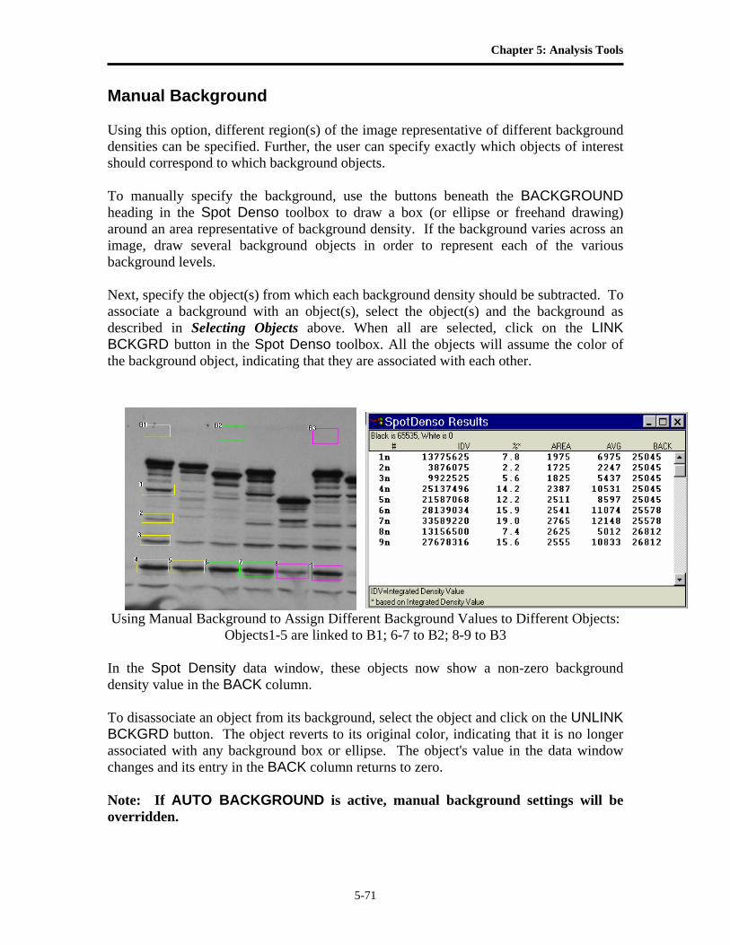
Chapter 5: Analysis Tools
5-71
Manual Background Using this option, different region(s) of the image representative of different background densities can be specified. Further, the user can specify exactly which objects of interest should correspond to which background objects. To manually specify the background, use the buttons beneath the BACKGROUND heading in the Spot Denso toolbox to draw a box (or ellipse or freehand drawing) around an area representative of background density. If the background varies across an image, draw several background objects in order to represent each of the various background levels. Next, specify the object(s) from which each background density should be subtracted. To associate a background with an object(s), select the object(s) and the background as described in Selecting Objects above. When all are selected, click on the LINK BCKGRD button in the Spot Denso toolbox. All the objects will assume the color of the background object, indicating that they are associated with each other.
Using Manual Background to Assign Different Background Values to Different Objects: Objects1-5 are linked to B1; 6-7 to B2; 8-9 to B3
In the Spot Density data window, these objects now show a non-zero background density value in the BACK column. To disassociate an object from its background, select the object and click on the UNLINK BCKGRD button. The object reverts to its original color, indicating that it is no longer associated with any background box or ellipse. The object's value in the data window changes and its entry in the BACK column returns to zero. Note: If AUTO BACKGROUND is active, manual background settings will be overridden.
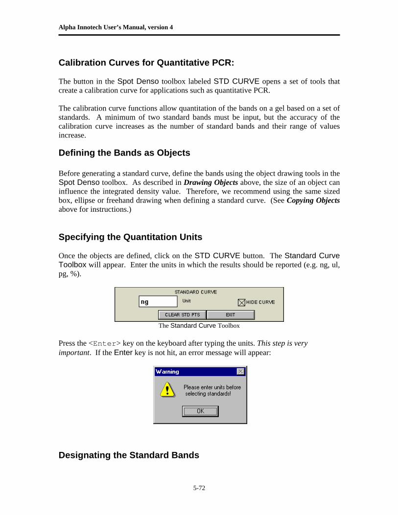
Alpha Innotech User’s Manual, version 4
5-72
Calibration Curves for Quantitative PCR: The button in the Spot Denso toolbox labeled STD CURVE opens a set of tools that create a calibration curve for applications such as quantitative PCR. The calibration curve functions allow quantitation of the bands on a gel based on a set of standards. A minimum of two standard bands must be input, but the accuracy of the calibration curve increases as the number of standard bands and their range of values increase.
Defining the Bands as Objects Before generating a standard curve, define the bands using the object drawing tools in the Spot Denso toolbox. As described in Drawing Objects above, the size of an object can influence the integrated density value. Therefore, we recommend using the same sized box, ellipse or freehand drawing when defining a standard curve. (See Copying Objects above for instructions.) Specifying the Quantitation Units Once the objects are defined, click on the STD CURVE button. The Standard Curve Toolbox will appear. Enter the units in which the results should be reported (e.g. ng, ul, pg, %).
The Standard Curve Toolbox
Press the <Enter> key on the keyboard after typing the units. This step is very important. If the Enter key is not hit, an error message will appear:
Designating the Standard Bands
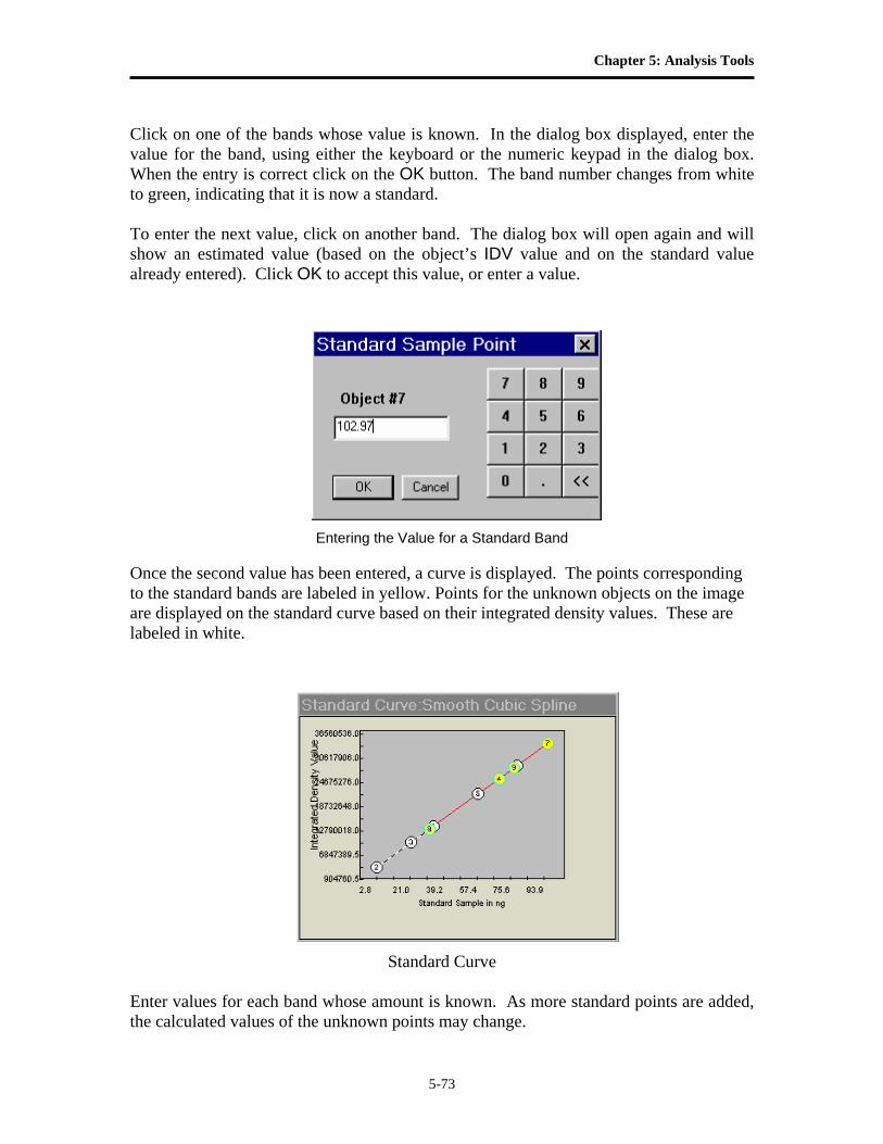
Chapter 5: Analysis Tools
5-73
Click on one of the bands whose value is known. In the dialog box displayed, enter the value for the band, using either the keyboard or the numeric keypad in the dialog box. When the entry is correct click on the OK button. The band number changes from white to green, indicating that it is now a standard. To enter the next value, click on another band. The dialog box will open again and will show an estimated value (based on the object’s IDV value and on the standard value already entered). Click OK to accept this value, or enter a value.
Entering the Value for a Standard Band
Once the second value has been entered, a curve is displayed. The points corresponding to the standard bands are labeled in yellow. Points for the unknown objects on the image are displayed on the standard curve based on their integrated density values. These are labeled in white.
Standard Curve Enter values for each band whose amount is known. As more standard points are added, the calculated values of the unknown points may change.
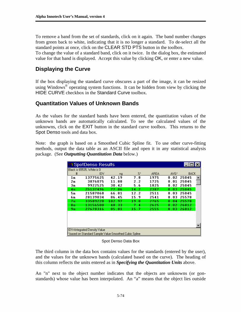
Alpha Innotech User’s Manual, version 4
5-74
To remove a band from the set of standards, click on it again. The band number changes from green back to white, indicating that it is no longer a standard. To de-select all the standard points at once, click on the CLEAR STD PTS button in the toolbox. To change the value of a standard band, click on it twice. In the dialog box, the estimated value for that band is displayed. Accept this value by clicking OK, or enter a new value.
Displaying the Curve If the box displaying the standard curve obscures a part of the image, it can be resized using Windows® operating system functions. It can be hidden from view by clicking the HIDE CURVE checkbox in the Standard Curve toolbox.
Quantitation Values of Unknown Bands As the values for the standard bands have been entered, the quantitation values of the unknown bands are automatically calculated. To see the calculated values of the unknowns, click on the EXIT button in the standard curve toolbox. This returns to the Spot Denso tools and data box. Note: the graph is based on a Smoothed Cubic Spline fit. To use other curve-fitting methods, output the data table as an ASCII file and open it in any statistical analysis package. (See Outputting Quantitation Data below.)
Spot Denso Data Box The third column in the data box contains values for the standards (entered by the user), and the values for the unknown bands (calculated based on the curve). The heading of this column reflects the units entered as in Specifying the Quantitation Units above. An "n" next to the object number indicates that the objects are unknowns (or non-standards) whose value has been interpolated. An “a” means that the object lies outside
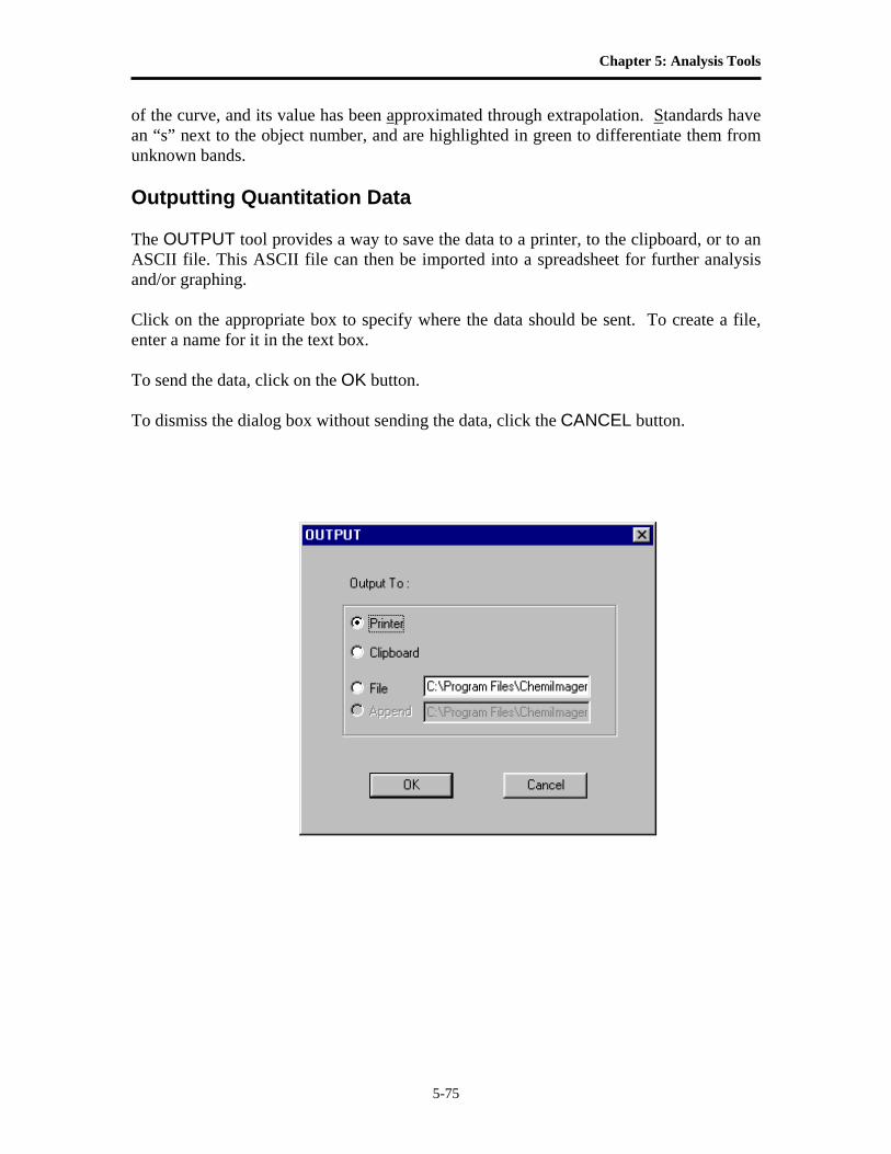
Chapter 5: Analysis Tools
5-75
of the curve, and its value has been approximated through extrapolation. Standards have an “s” next to the object number, and are highlighted in green to differentiate them from unknown bands. Outputting Quantitation Data The OUTPUT tool provides a way to save the data to a printer, to the clipboard, or to an ASCII file. This ASCII file can then be imported into a spreadsheet for further analysis and/or graphing. Click on the appropriate box to specify where the data should be sent. To create a file, enter a name for it in the text box. To send the data, click on the OK button. To dismiss the dialog box without sending the data, click the CANCEL button.
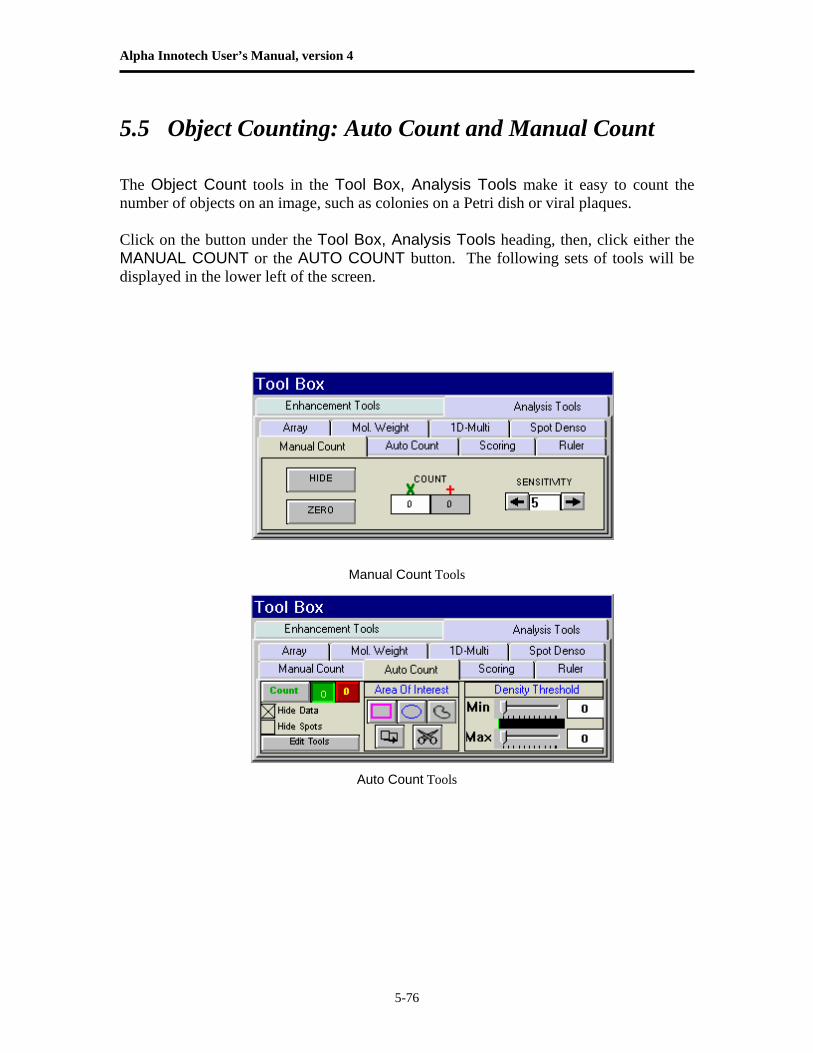
Alpha Innotech User’s Manual, version 4
5-76
5.5 Object Counting: Auto Count and Manual Count The Object Count tools in the Tool Box, Analysis Tools make it easy to count the number of objects on an image, such as colonies on a Petri dish or viral plaques. Click on the button under the Tool Box, Analysis Tools heading, then, click either the MANUAL COUNT or the AUTO COUNT button. The following sets of tools will be displayed in the lower left of the screen.
Manual Count Tools
Auto Count Tools
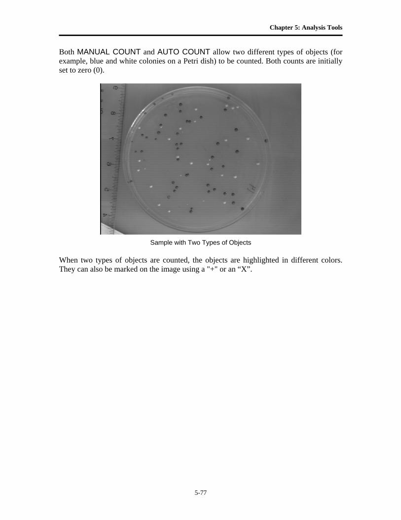
Chapter 5: Analysis Tools
5-77
Both MANUAL COUNT and AUTO COUNT allow two different types of objects (for example, blue and white colonies on a Petri dish) to be counted. Both counts are initially set to zero (0).
Sample with Two Types of Objects
When two types of objects are counted, the objects are highlighted in different colors. They can also be marked on the image using a "+" or an “X”.
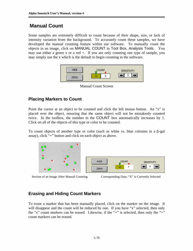
Alpha Innotech User’s Manual, version 4
5-78
Manual Count Some samples are extremely difficult to count because of their shape, size, or lack of intensity variation from the background. To accurately count these samples, we have developed the manual counting feature within our software. To manually count the objects in an image, click on MANUAL COUNT in Tool Box, Analysis Tools. You may use either a green x or a red +. If you are only counting one type of sample, you may simply use the x which is the default to begin counting in the software.
Manual Count Screen
Placing Markers to Count Point the cursor at an object to be counted and click the left mouse button. An “x” is placed over the object, ensuring that the same object will not be mistakenly counted twice. In the toolbox, the number in the COUNT box automatically increases by 1. Click on all of the objects of this type or color to be counted. To count objects of another type or color (such as white vs. blue colonies in a β-gal assay), click “+” button and click on each object as above.
Section of an Image After Manual Counting Corresponding Data; “X” is Currently Selected
Erasing and Hiding Count Markers To erase a marker that has been manually placed, click on the marker on the image. It will disappear and the count will be reduced by one. If you have “x” selected, then only the “x” count markers can be erased. Likewise, if the “+” is selected, then only the “+” count markers can be erased.
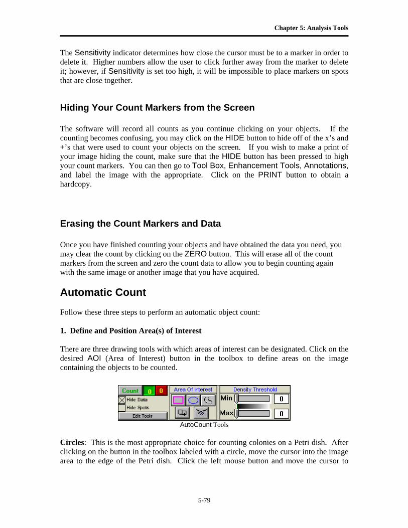
Chapter 5: Analysis Tools
5-79
The Sensitivity indicator determines how close the cursor must be to a marker in order to delete it. Higher numbers allow the user to click further away from the marker to delete it; however, if Sensitivity is set too high, it will be impossible to place markers on spots that are close together.
Hiding Your Count Markers from the Screen The software will record all counts as you continue clicking on your objects. If the counting becomes confusing, you may click on the HIDE button to hide off of the x’s and +’s that were used to count your objects on the screen. If you wish to make a print of your image hiding the count, make sure that the HIDE button has been pressed to high your count markers. You can then go to Tool Box, Enhancement Tools, Annotations, and label the image with the appropriate. Click on the PRINT button to obtain a hardcopy.
Erasing the Count Markers and Data Once you have finished counting your objects and have obtained the data you need, you may clear the count by clicking on the ZERO button. This will erase all of the count markers from the screen and zero the count data to allow you to begin counting again with the same image or another image that you have acquired. Automatic Count Follow these three steps to perform an automatic object count: 1. Define and Position Area(s) of Interest There are three drawing tools with which areas of interest can be designated. Click on the desired AOI (Area of Interest) button in the toolbox to define areas on the image containing the objects to be counted.
AutoCount Tools
Circles: This is the most appropriate choice for counting colonies on a Petri dish. After clicking on the button in the toolbox labeled with a circle, move the cursor into the image area to the edge of the Petri dish. Click the left mouse button and move the cursor to
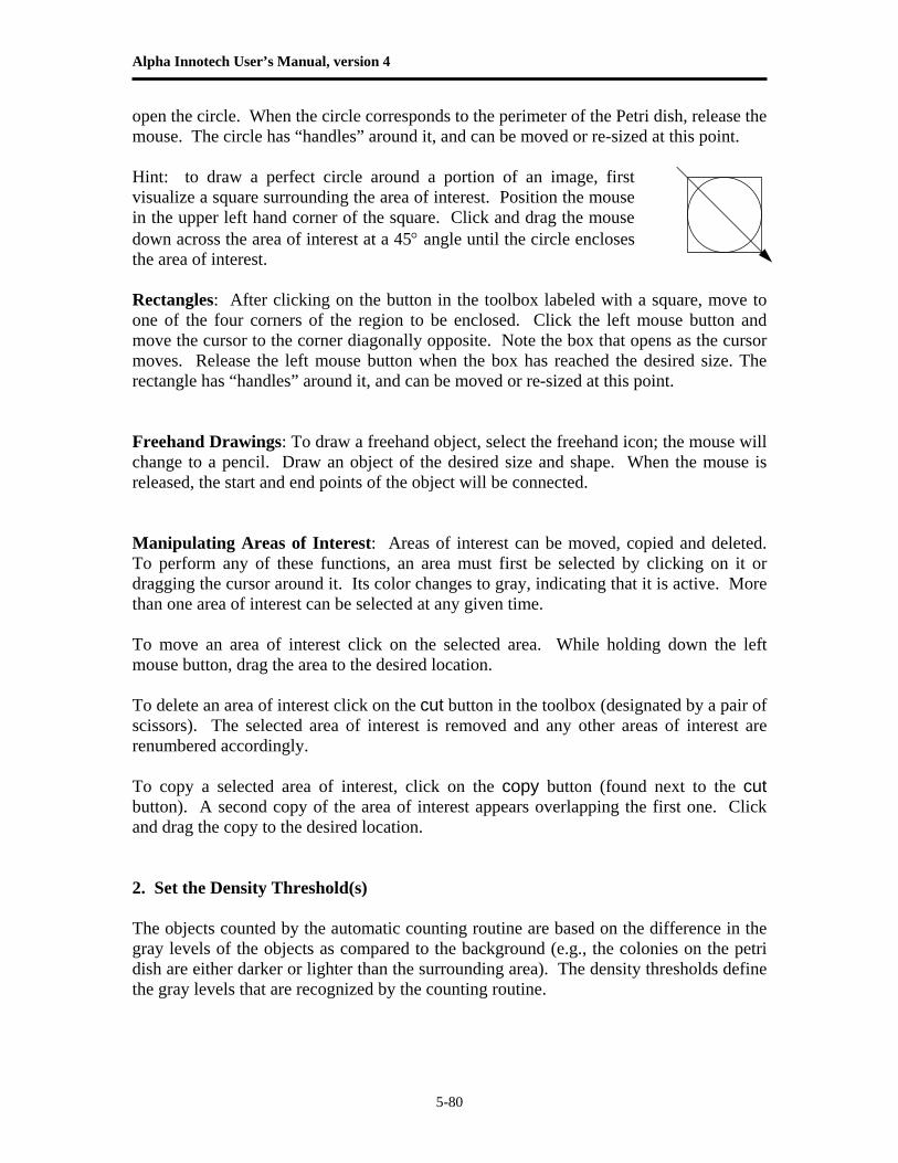
Alpha Innotech User’s Manual, version 4
5-80
open the circle. When the circle corresponds to the perimeter of the Petri dish, release the mouse. The circle has “handles” around it, and can be moved or re-sized at this point. Hint: to draw a perfect circle around a portion of an image, first visualize a square surrounding the area of interest. Position the mouse in the upper left hand corner of the square. Click and drag the mouse down across the area of interest at a 45° angle until the circle encloses the area of interest. Rectangles: After clicking on the button in the toolbox labeled with a square, move to one of the four corners of the region to be enclosed. Click the left mouse button and move the cursor to the corner diagonally opposite. Note the box that opens as the cursor moves. Release the left mouse button when the box has reached the desired size. The rectangle has “handles” around it, and can be moved or re-sized at this point. Freehand Drawings: To draw a freehand object, select the freehand icon; the mouse will change to a pencil. Draw an object of the desired size and shape. When the mouse is released, the start and end points of the object will be connected. Manipulating Areas of Interest: Areas of interest can be moved, copied and deleted. To perform any of these functions, an area must first be selected by clicking on it or dragging the cursor around it. Its color changes to gray, indicating that it is active. More than one area of interest can be selected at any given time. To move an area of interest click on the selected area. While holding down the left mouse button, drag the area to the desired location. To delete an area of interest click on the cut button in the toolbox (designated by a pair of scissors). The selected area of interest is removed and any other areas of interest are renumbered accordingly. To copy a selected area of interest, click on the copy button (found next to the cut button). A second copy of the area of interest appears overlapping the first one. Click and drag the copy to the desired location. 2. Set the Density Threshold(s) The objects counted by the automatic counting routine are based on the difference in the gray levels of the objects as compared to the background (e.g., the colonies on the petri dish are either darker or lighter than the surrounding area). The density thresholds define the gray levels that are recognized by the counting routine.
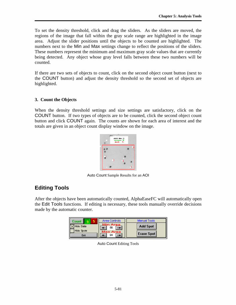
Chapter 5: Analysis Tools
5-81
To set the density threshold, click and drag the sliders. As the sliders are moved, the regions of the image that fall within the gray scale range are highlighted in the image area. Adjust the slider positions until the objects to be counted are highlighted. The numbers next to the Min and Max settings change to reflect the positions of the sliders. These numbers represent the minimum and maximum gray scale values that are currently being detected. Any object whose gray level falls between these two numbers will be counted. If there are two sets of objects to count, click on the second object count button (next to the COUNT button) and adjust the density threshold so the second set of objects are highlighted. 3. Count the Objects When the density threshold settings and size settings are satisfactory, click on the COUNT button. If two types of objects are to be counted, click the second object count button and click COUNT again. The counts are shown for each area of interest and the totals are given in an object count display window on the image.
Auto Count Sample Results for an AOI
Editing Tools After the objects have been automatically counted, AlphaEaseFC will automatically open the Edit Tools functions. If editing is necessary, these tools manually override decisions made by the automatic counter.
Auto Count Editing Tools
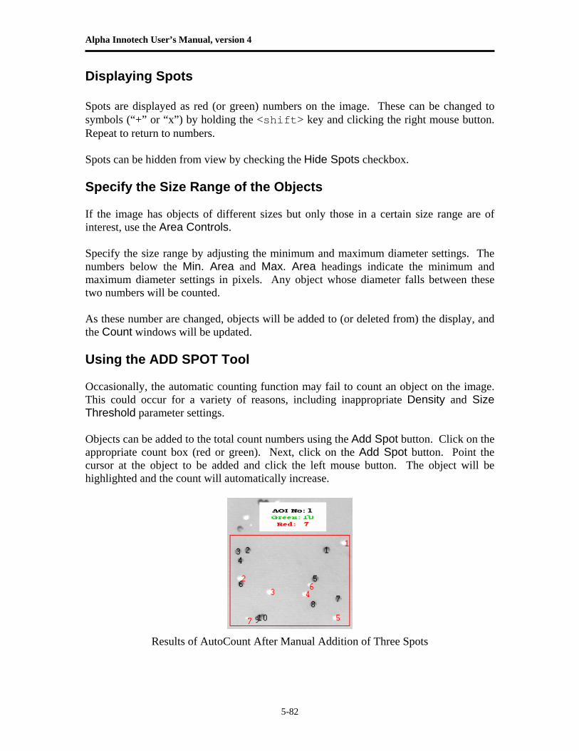
Alpha Innotech User’s Manual, version 4
5-82
Displaying Spots Spots are displayed as red (or green) numbers on the image. These can be changed to symbols (“+” or “x”) by holding the <shift> key and clicking the right mouse button. Repeat to return to numbers. Spots can be hidden from view by checking the Hide Spots checkbox. Specify the Size Range of the Objects If the image has objects of different sizes but only those in a certain size range are of interest, use the Area Controls. Specify the size range by adjusting the minimum and maximum diameter settings. The numbers below the Min. Area and Max. Area headings indicate the minimum and maximum diameter settings in pixels. Any object whose diameter falls between these two numbers will be counted. As these number are changed, objects will be added to (or deleted from) the display, and the Count windows will be updated. Using the ADD SPOT Tool Occasionally, the automatic counting function may fail to count an object on the image. This could occur for a variety of reasons, including inappropriate Density and Size Threshold parameter settings. Objects can be added to the total count numbers using the Add Spot button. Click on the appropriate count box (red or green). Next, click on the Add Spot button. Point the cursor at the object to be added and click the left mouse button. The object will be highlighted and the count will automatically increase.
Results of AutoCount After Manual Addition of Three Spots
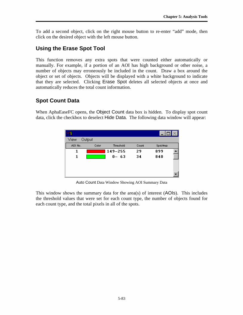
Chapter 5: Analysis Tools
5-83
To add a second object, click on the right mouse button to re-enter “add” mode, then click on the desired object with the left mouse button. Using the Erase Spot Tool This function removes any extra spots that were counted either automatically or manually. For example, if a portion of an AOI has high background or other noise, a number of objects may erroneously be included in the count. Draw a box around the object or set of objects. Objects will be displayed with a white background to indicate that they are selected. Clicking Erase Spot deletes all selected objects at once and automatically reduces the total count information. Spot Count Data When AphaEaseFC opens, the Object Count data box is hidden. To display spot count data, click the checkbox to deselect Hide Data. The following data window will appear:
Auto Count Data Window Showing AOI Summary Data This window shows the summary data for the area(s) of interest (AOIs). This includes the threshold values that were set for each count type, the number of objects found for each count type, and the total pixels in all of the spots.
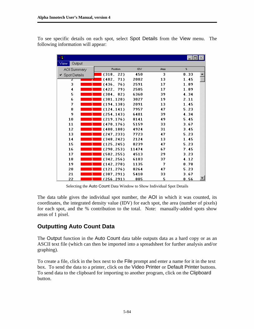
Alpha Innotech User’s Manual, version 4
5-84
To see specific details on each spot, select Spot Details from the View menu. The following information will appear:
Selecting the Auto Count Data Window to Show Individual Spot Details
The data table gives the individual spot number, the AOI in which it was counted, its coordinates, the integrated density value (IDV) for each spot, the area (number of pixels) for each spot, and the % contribution to the total. Note: manually-added spots show areas of 1 pixel. Outputting Auto Count Data The Output function in the Auto Count data table outputs data as a hard copy or as an ASCII text file (which can then be imported into a spreadsheet for further analysis and/or graphing). To create a file, click in the box next to the File prompt and enter a name for it in the text box. To send the data to a printer, click on the Video Printer or Default Printer buttons. To send data to the clipboard for importing to another program, click on the Clipboard button.
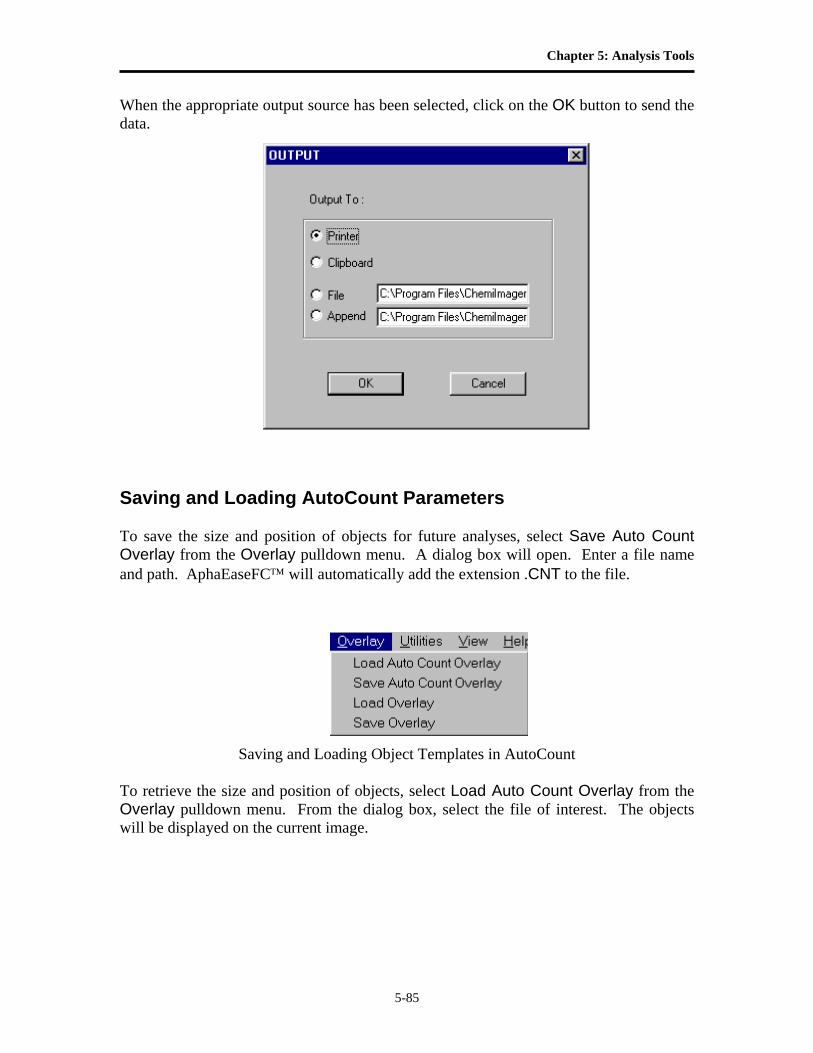
Chapter 5: Analysis Tools
5-85
When the appropriate output source has been selected, click on the OK button to send the data.
Saving and Loading AutoCount Parameters To save the size and position of objects for future analyses, select Save Auto Count Overlay from the Overlay pulldown menu. A dialog box will open. Enter a file name and path. AphaEaseFC™ will automatically add the extension .CNT to the file.
Saving and Loading Object Templates in AutoCount To retrieve the size and position of objects, select Load Auto Count Overlay from the Overlay pulldown menu. From the dialog box, select the file of interest. The objects will be displayed on the current image.
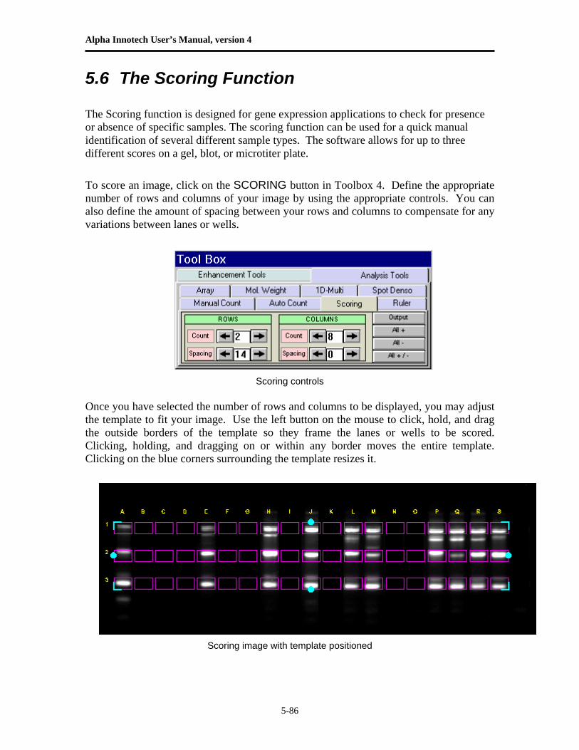
Alpha Innotech User’s Manual, version 4
5-86
5.6 The Scoring Function The Scoring function is designed for gene expression applications to check for presence or absence of specific samples. The scoring function can be used for a quick manual identification of several different sample types. The software allows for up to three different scores on a gel, blot, or microtiter plate.
To score an image, click on the SCORING button in Toolbox 4. Define the appropriate number of rows and columns of your image by using the appropriate controls. You can also define the amount of spacing between your rows and columns to compensate for any variations between lanes or wells.
Scoring controls Once you have selected the number of rows and columns to be displayed, you may adjust the template to fit your image. Use the left button on the mouse to click, hold, and drag the outside borders of the template so they frame the lanes or wells to be scored. Clicking, holding, and dragging on or within any border moves the entire template. Clicking on the blue corners surrounding the template resizes it.
Scoring image with template positioned
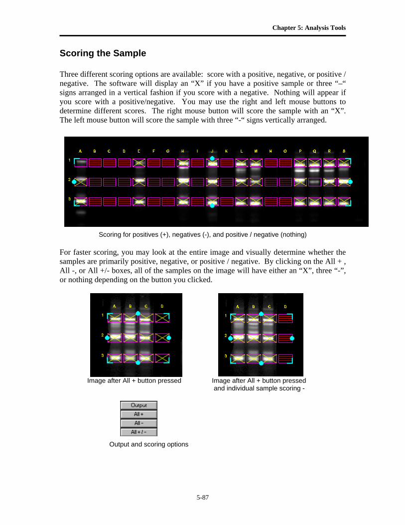
Chapter 5: Analysis Tools
5-87
Scoring the Sample Three different scoring options are available: score with a positive, negative, or positive / negative. The software will display an “X” if you have a positive sample or three “–“ signs arranged in a vertical fashion if you score with a negative. Nothing will appear if you score with a positive/negative. You may use the right and left mouse buttons to determine different scores. The right mouse button will score the sample with an “X”. The left mouse button will score the sample with three “-“ signs vertically arranged.
Scoring for positives (+), negatives (-), and positive / negative (nothing) For faster scoring, you may look at the entire image and visually determine whether the samples are primarily positive, negative, or positive / negative. By clicking on the All + , All -, or All +/- boxes, all of the samples on the image will have either an “X”, three “-”, or nothing depending on the button you clicked.
Image after All + button pressed Image after All + button pressed and individual sample scoring -
Output and scoring options
Alpha Innotech User’s Manual, version 4
5-88
Outputting Scoring Results Once you have completed scoring your sample, you may output the results. The results can either be printed directly to a printer, or you may export the results as ASCII data for direct importation into Excel or other spreadsheet programs Sending a Screen Image to a Printer Click on the PRINT button on the software interface to printout your image with the scoring marks. Sending Data to a Printer To send the data directly to the Video Printer or Default Printer, click on the OUTPUT button and click in the circle next to appropriate printer. Clicking on the OK button will send the data directly to the printer attached to your imaging system. Sending Data to a Spreadsheet Program To send the data results to Excel or other spreadsheet programs, click on the OUTPUT button, click on the clipboard option, then click on OK. If you have Excel or another spreadsheet program loaded on the system and running in the background, you can simply press the ALT and TAB keys simultaneously to move into the spreadsheet program. You can then import the data directly to the desired spreadsheet from clipboard. Note: The spreadsheet program must be installed on the computer in order to output the data to that program. Sending Data to a File If you would like to take the data from the system and import it into another computer, the data can be saved to a diskette or network which will allow you to open the data file on a separate workstation connected to the network. Click on the OUTPUT button and then on the File option. Specify the path and file name to send the data file. The data is saved as an ASCII file and can be imported into most spreadsheet programs. ASCII is a very common file format output option for numerical data.
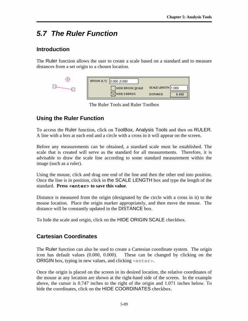
Chapter 5: Analysis Tools
5-89
5.7 The Ruler Function Introduction The Ruler function allows the user to create a scale based on a standard and to measure distances from a set origin to a chosen location.
The Ruler Tools and Ruler Toolbox
Using the Ruler Function To access the Ruler function, click on ToolBox, Analysis Tools and then on RULER. A line with a box at each end and a circle with a cross in it will appear on the screen. Before any measurements can be obtained, a standard scale must be established. The scale that is created will serve as the standard for all measurements. Therefore, it is advisable to draw the scale line according to some standard measurement within the image (such as a ruler). Using the mouse, click and drag one end of the line and then the other end into position. Once the line is in position, click in the SCALE LENGTH box and type the length of the standard. Press <enter> to save this value. Distance is measured from the origin (designated by the circle with a cross in it) to the mouse location. Place the origin marker appropriately, and then move the mouse. The distance will be constantly updated in the DISTANCE box. To hide the scale and origin, click on the HIDE ORIGIN SCALE checkbox.
Cartesian Coordinates The Ruler function can also be used to create a Cartesian coordinate system. The origin icon has default values (0.000, 0.000). These can be changed by clicking on the ORIGIN box, typing in new values, and clicking <enter>. Once the origin is placed on the screen in its desired location, the relative coordinates of the mouse at any location are shown at the right-hand side of the screen. In the example above, the cursor is 0.747 inches to the right of the origin and 1.071 inches below. To hide the coordinates, click on the HIDE COORDINATES checkbox.

Alpha Innotech User’s Manual, version 4
5-90
BLANK PAGE
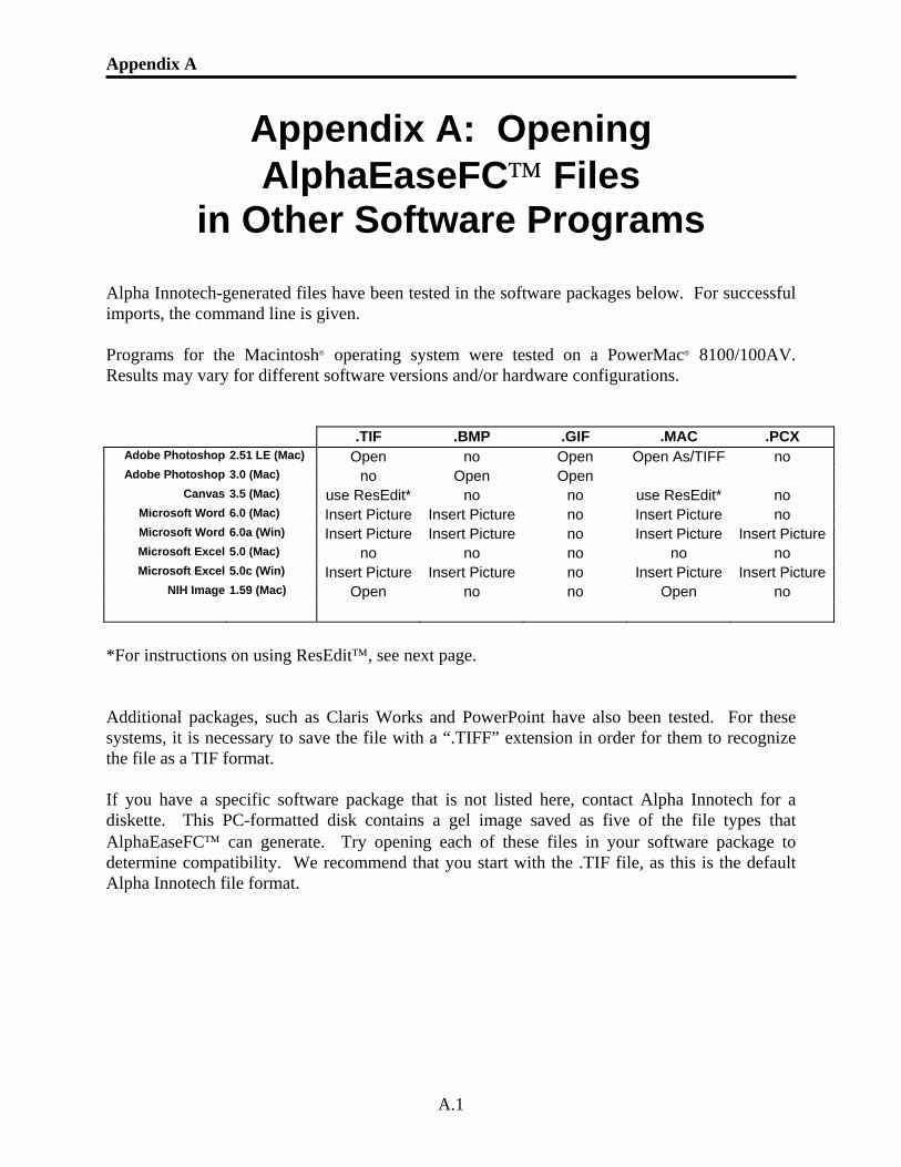
Appendix A
A.1
Appendix A: Opening AlphaEaseFC™ Files
in Other Software Programs Alpha Innotech-generated files have been tested in the software packages below. For successful imports, the command line is given. Programs for the Macintosh® operating system were tested on a PowerMac® 8100/100AV. Results may vary for different software versions and/or hardware configurations.
.TIF .BMP .GIF .MAC .PCX Adobe Photoshop 2.51 LE (Mac) Open no Open Open As/TIFF no Adobe Photoshop 3.0 (Mac) no Open Open
Canvas 3.5 (Mac) use ResEdit* no no use ResEdit* no Microsoft Word 6.0 (Mac) Insert Picture Insert Picture no Insert Picture no Microsoft Word 6.0a (Win) Insert Picture Insert Picture no Insert Picture Insert PictureMicrosoft Excel 5.0 (Mac) no no no no no Microsoft Excel 5.0c (Win) Insert Picture Insert Picture no Insert Picture Insert Picture
NIH Image 1.59 (Mac) Open no no Open no
*For instructions on using ResEdit™, see next page. Additional packages, such as Claris Works and PowerPoint have also been tested. For these systems, it is necessary to save the file with a “.TIFF” extension in order for them to recognize the file as a TIF format. If you have a specific software package that is not listed here, contact Alpha Innotech for a diskette. This PC-formatted disk contains a gel image saved as five of the file types that AlphaEaseFC™ can generate. Try opening each of these files in your software package to determine compatibility. We recommend that you start with the .TIF file, as this is the default Alpha Innotech file format.
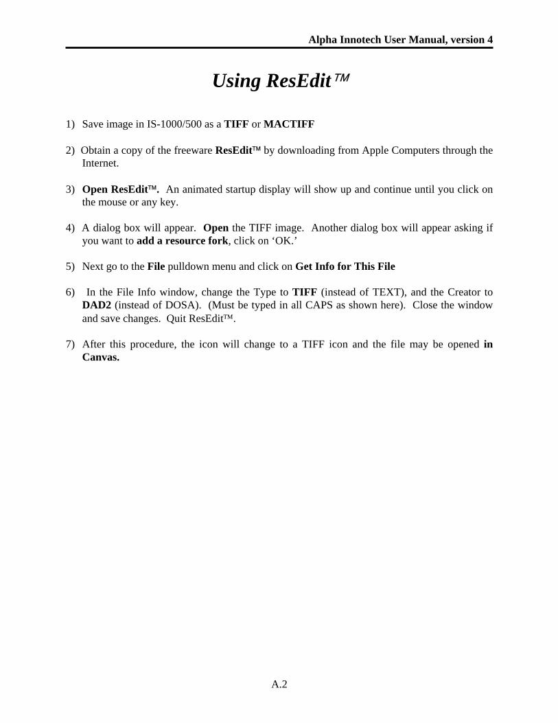
Alpha Innotech User Manual, version 4
A.2
Using ResEdit™ 1) Save image in IS-1000/500 as a TIFF or MACTIFF 2) Obtain a copy of the freeware ResEdit™ by downloading from Apple Computers through the
Internet. 3) Open ResEdit™. An animated startup display will show up and continue until you click on
the mouse or any key. 4) A dialog box will appear. Open the TIFF image. Another dialog box will appear asking if
you want to add a resource fork, click on ‘OK.’ 5) Next go to the File pulldown menu and click on Get Info for This File 6) In the File Info window, change the Type to TIFF (instead of TEXT), and the Creator to
DAD2 (instead of DOSA). (Must be typed in all CAPS as shown here). Close the window and save changes. Quit ResEdit™.
7) After this procedure, the icon will change to a TIFF icon and the file may be opened in
Canvas.
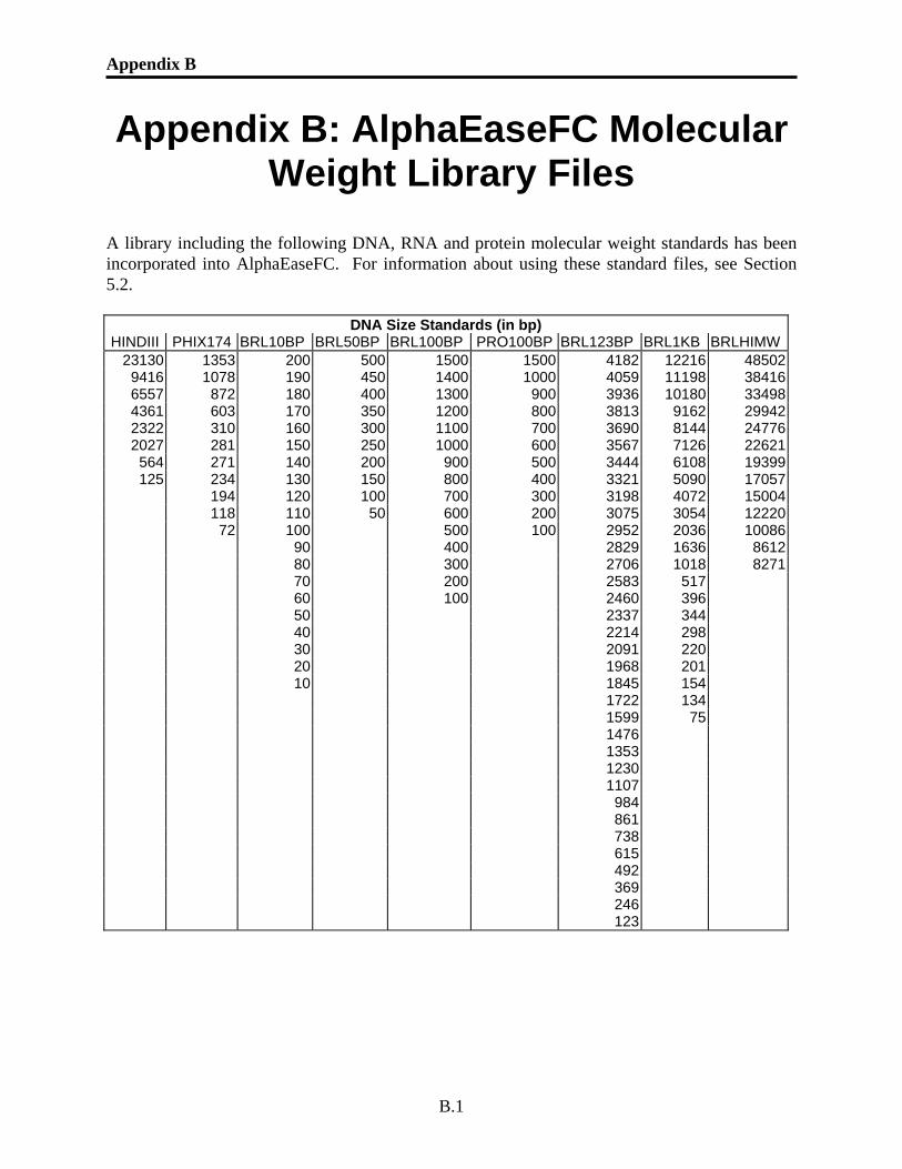
Appendix B
B.1
Appendix B: AlphaEaseFC Molecular Weight Library Files
A library including the following DNA, RNA and protein molecular weight standards has been incorporated into AlphaEaseFC. For information about using these standard files, see Section 5.2.
DNA Size Standards (in bp) HINDIII PHIX174 BRL10BP BRL50BP BRL100BP PRO100BP BRL123BP BRL1KB BRLHIMW
23130 1353 200 500 1500 1500 4182 12216 485029416 1078 190 450 1400 1000 4059 11198 384166557 872 180 400 1300 900 3936 10180 334984361 603 170 350 1200 800 3813 9162 299422322 310 160 300 1100 700 3690 8144 247762027 281 150 250 1000 600 3567 7126 22621
564 271 140 200 900 500 3444 6108 19399125 234 130 150 800 400 3321 5090 17057
194 120 100 700 300 3198 4072 15004 118 110 50 600 200 3075 3054 12220 72 100 500 100 2952 2036 10086 90 400 2829 1636 8612 80 300 2706 1018 8271 70 200 2583 517 60 100 2460 396 50 2337 344 40 2214 298 30 2091 220 20 1968 201 10 1845 154 1722 134 1599 75 1476 1353 1230 1107 984 861 738 615 492 369 246 123
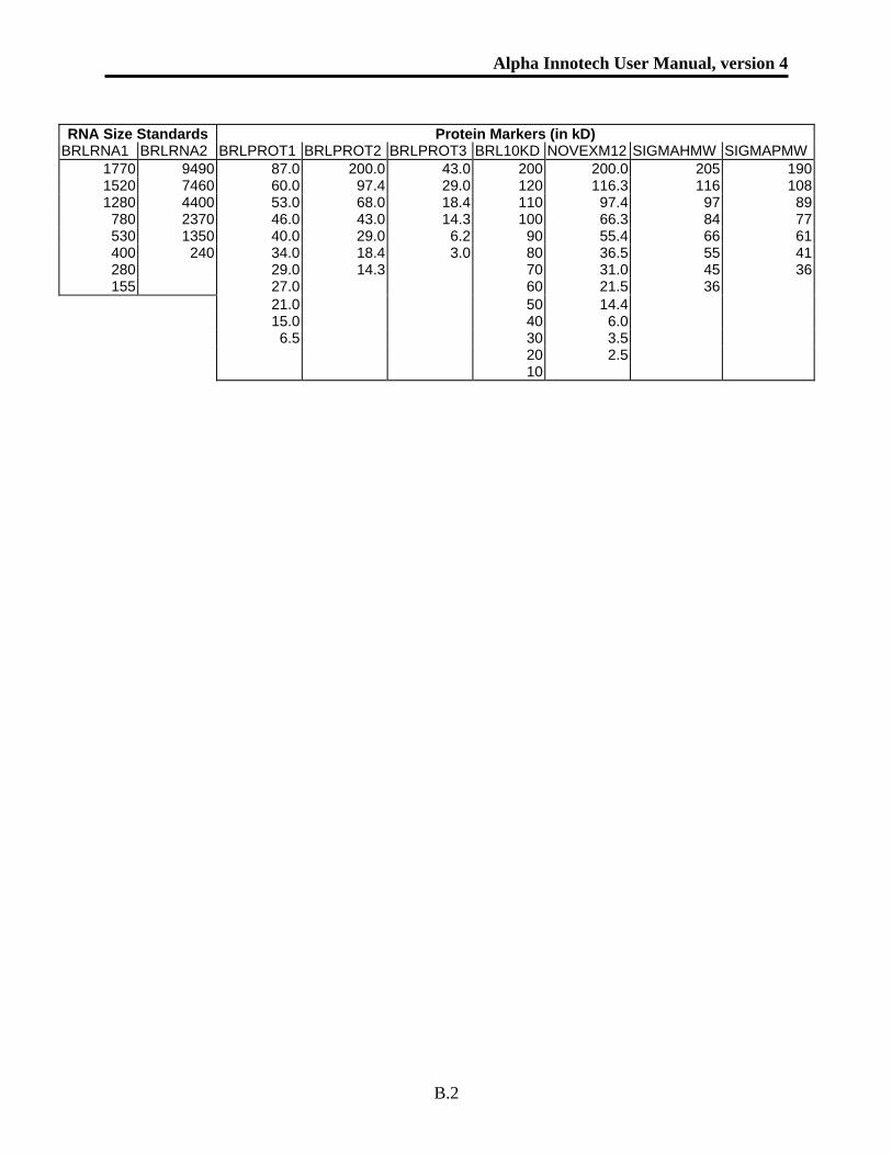
Alpha Innotech User Manual, version 4
B.2
RNA Size Standards Protein Markers (in kD)
BRLRNA1 BRLRNA2 BRLPROT1 BRLPROT2 BRLPROT3 BRL10KD NOVEXM12 SIGMAHMW SIGMAPMW1770 9490 87.0 200.0 43.0 200 200.0 205 1901520 7460 60.0 97.4 29.0 120 116.3 116 1081280 4400 53.0 68.0 18.4 110 97.4 97 89
780 2370 46.0 43.0 14.3 100 66.3 84 77530 1350 40.0 29.0 6.2 90 55.4 66 61400 240 34.0 18.4 3.0 80 36.5 55 41280 29.0 14.3 70 31.0 45 36155 27.0 60 21.5 36
21.0 50 14.4 15.0 40 6.0 6.5 30 3.5 20 2.5 10
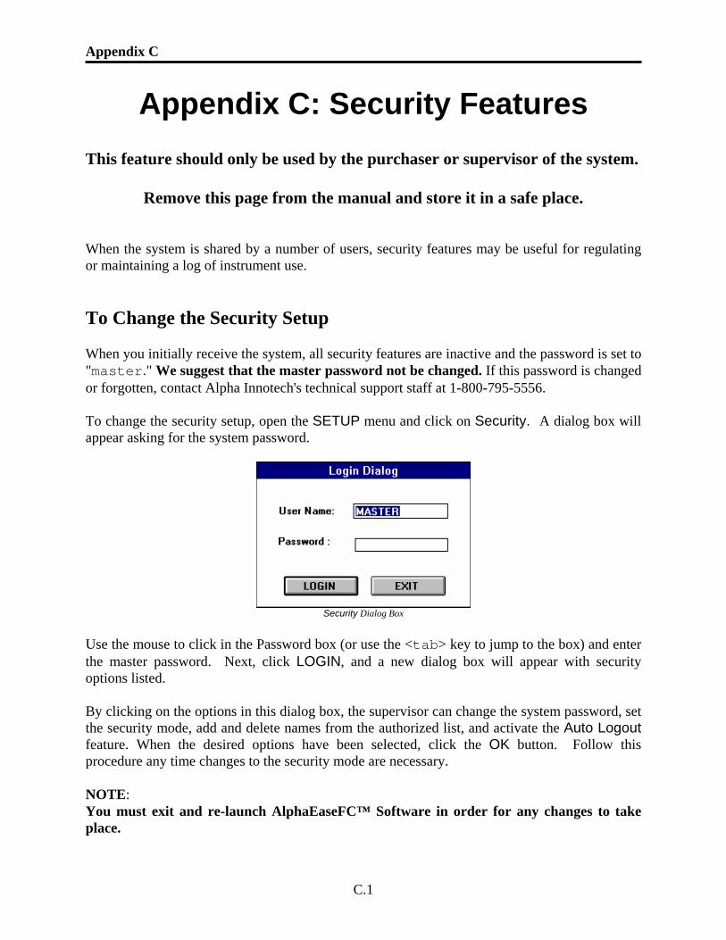
Appendix C
C.1
Appendix C: Security Features This feature should only be used by the purchaser or supervisor of the system.
Remove this page from the manual and store it in a safe place. When the system is shared by a number of users, security features may be useful for regulating or maintaining a log of instrument use. To Change the Security Setup When you initially receive the system, all security features are inactive and the password is set to "master." We suggest that the master password not be changed. If this password is changed or forgotten, contact Alpha Innotech's technical support staff at 1-800-795-5556. To change the security setup, open the SETUP menu and click on Security. A dialog box will appear asking for the system password.
Security Dialog Box
Use the mouse to click in the Password box (or use the <tab> key to jump to the box) and enter the master password. Next, click LOGIN, and a new dialog box will appear with security options listed. By clicking on the options in this dialog box, the supervisor can change the system password, set the security mode, add and delete names from the authorized list, and activate the Auto Logout feature. When the desired options have been selected, click the OK button. Follow this procedure any time changes to the security mode are necessary. NOTE: You must exit and re-launch AlphaEaseFC™ Software in order for any changes to take place.
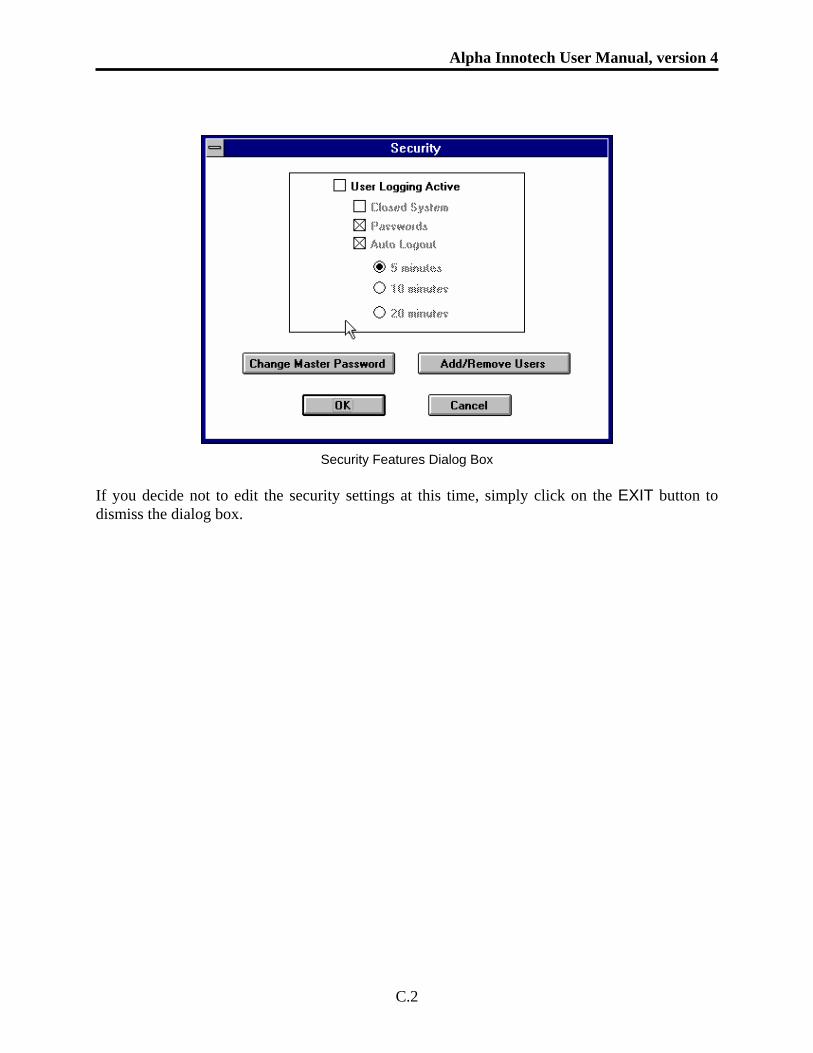
Alpha Innotech User Manual, version 4
C.2
Security Features Dialog Box If you decide not to edit the security settings at this time, simply click on the EXIT button to dismiss the dialog box.
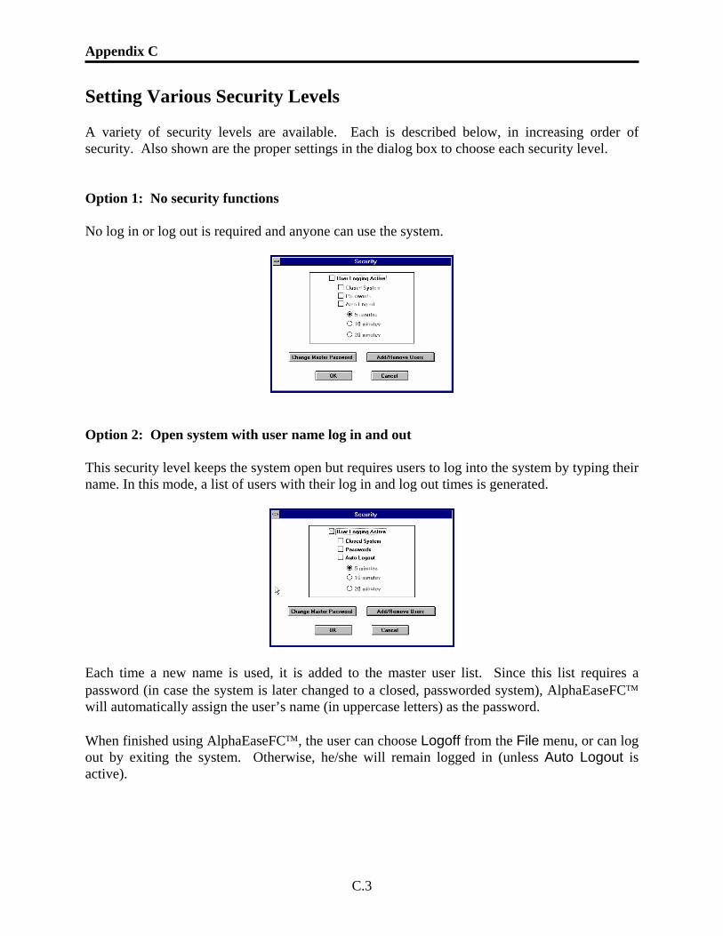
Appendix C
C.3
Setting Various Security Levels A variety of security levels are available. Each is described below, in increasing order of security. Also shown are the proper settings in the dialog box to choose each security level. Option 1: No security functions No log in or log out is required and anyone can use the system.
Option 2: Open system with user name log in and out This security level keeps the system open but requires users to log into the system by typing their name. In this mode, a list of users with their log in and log out times is generated.
Each time a new name is used, it is added to the master user list. Since this list requires a password (in case the system is later changed to a closed, passworded system), AlphaEaseFC™ will automatically assign the user’s name (in uppercase letters) as the password. When finished using AlphaEaseFC™, the user can choose Logoff from the File menu, or can log out by exiting the system. Otherwise, he/she will remain logged in (unless Auto Logout is active).
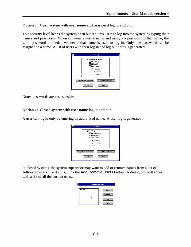
Alpha Innotech User Manual, version 4
C.4
Option 3: Open system with user name and password log in and out This security level keeps the system open but requires users to log into the system by typing their names and passwords. When someone enters a name and assigns a password to that name, the same password is needed whenever that name is used to log in. Only one password can be assigned to a name. A list of users with their log in and log out times is generated.
Note: passwords are case sensitive. Option 4: Closed system with user name log in and out A user can log in only by entering an authorized name. A user log is generated.
In closed systems, the system supervisor may want to add or remove names from a list of authorized users. To do this, click the Add/Remove Users button. A dialog box will appear with a list of all the current users.
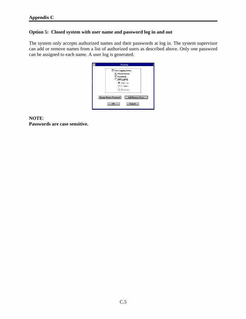
Appendix C
C.5
Option 5: Closed system with user name and password log in and out The system only accepts authorized names and their passwords at log in. The system supervisor can add or remove names from a list of authorized users as described above. Only one password can be assigned to each name. A user log is generated.
NOTE: Passwords are case sensitive.

Alpha Innotech User Manual, version 4
C.6
BLANK PAGE
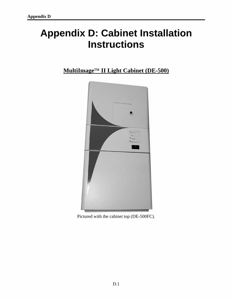
Appendix D
D.1
Appendix D: Cabinet Installation Instructions
MultiImage™ II Light Cabinet (DE-500)
Pictured with the cabinet top (DE-500FC).
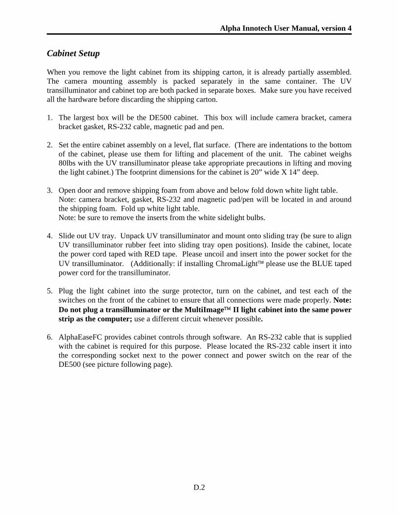
Alpha Innotech User Manual, version 4
D.2
Cabinet Setup When you remove the light cabinet from its shipping carton, it is already partially assembled. The camera mounting assembly is packed separately in the same container. The UV transilluminator and cabinet top are both packed in separate boxes. Make sure you have received all the hardware before discarding the shipping carton. 1. The largest box will be the DE500 cabinet. This box will include camera bracket, camera
bracket gasket, RS-232 cable, magnetic pad and pen. 2. Set the entire cabinet assembly on a level, flat surface. (There are indentations to the bottom
of the cabinet, please use them for lifting and placement of the unit. The cabinet weighs 80lbs with the UV transilluminator please take appropriate precautions in lifting and moving the light cabinet.) The footprint dimensions for the cabinet is 20” wide X 14” deep.
3. Open door and remove shipping foam from above and below fold down white light table.
Note: camera bracket, gasket, RS-232 and magnetic pad/pen will be located in and around the shipping foam. Fold up white light table. Note: be sure to remove the inserts from the white sidelight bulbs.
4. Slide out UV tray. Unpack UV transilluminator and mount onto sliding tray (be sure to align
UV transilluminator rubber feet into sliding tray open positions). Inside the cabinet, locate the power cord taped with RED tape. Please uncoil and insert into the power socket for the UV transilluminator. (Additionally: if installing ChromaLight™ please use the BLUE taped power cord for the transilluminator.
5. Plug the light cabinet into the surge protector, turn on the cabinet, and test each of the
switches on the front of the cabinet to ensure that all connections were made properly. Note: Do not plug a transilluminator or the MultiImage™ II light cabinet into the same power strip as the computer; use a different circuit whenever possible.
6. AlphaEaseFC provides cabinet controls through software. An RS-232 cable that is supplied
with the cabinet is required for this purpose. Please located the RS-232 cable insert it into the corresponding socket next to the power connect and power switch on the rear of the DE500 (see picture following page).
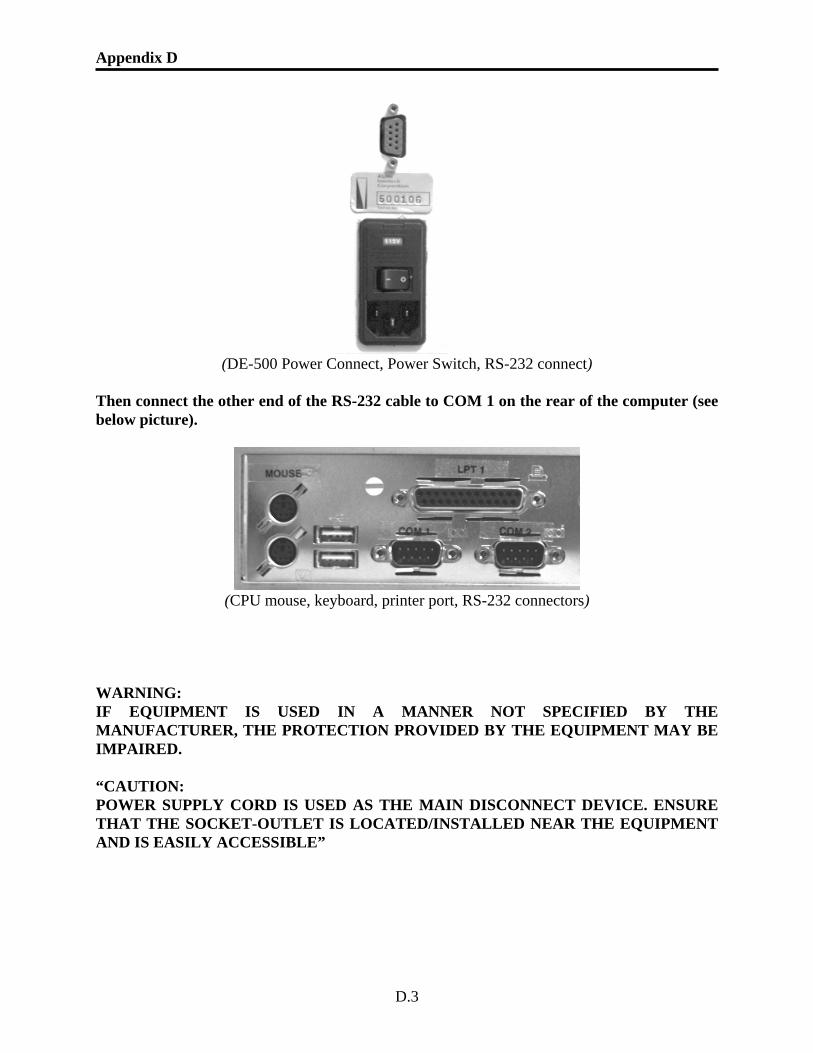
Appendix D
D.3
(DE-500 Power Connect, Power Switch, RS-232 connect)
Then connect the other end of the RS-232 cable to COM 1 on the rear of the computer (see below picture).
(CPU mouse, keyboard, printer port, RS-232 connectors)
WARNING: IF EQUIPMENT IS USED IN A MANNER NOT SPECIFIED BY THE MANUFACTURER, THE PROTECTION PROVIDED BY THE EQUIPMENT MAY BE IMPAIRED. “CAUTION: POWER SUPPLY CORD IS USED AS THE MAIN DISCONNECT DEVICE. ENSURE THAT THE SOCKET-OUTLET IS LOCATED/INSTALLED NEAR THE EQUIPMENT AND IS EASILY ACCESSIBLE”
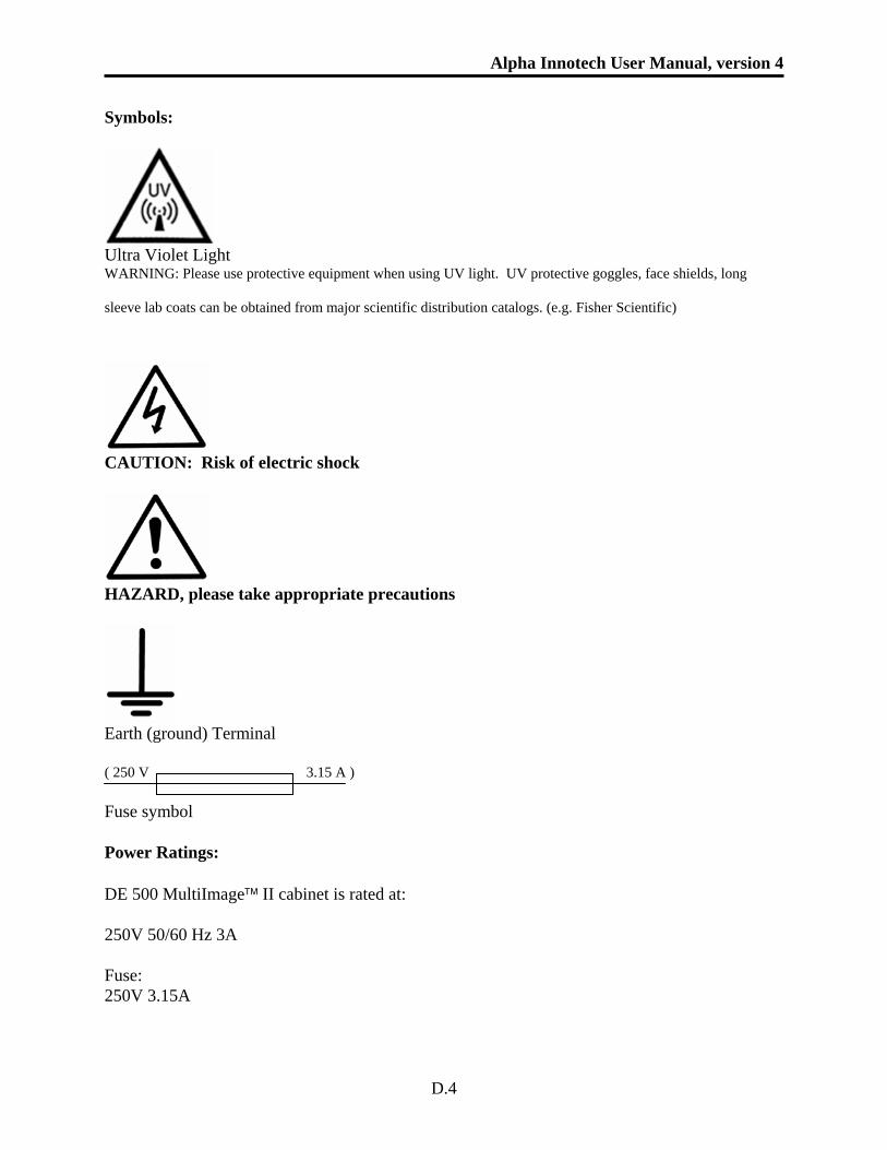
Alpha Innotech User Manual, version 4
D.4
Symbols:
Ultra Violet Light WARNING: Please use protective equipment when using UV light. UV protective goggles, face shields, long
sleeve lab coats can be obtained from major scientific distribution catalogs. (e.g. Fisher Scientific)
CAUTION: Risk of electric shock
HAZARD, please take appropriate precautions
Earth (ground) Terminal ( 250 V 3.15 A ) Fuse symbol Power Ratings: DE 500 MultiImage™ II cabinet is rated at: 250V 50/60 Hz 3A Fuse: 250V 3.15A
Appendix D
D.5
Camera Installation 1. Write down the position of each filter on the magnetic notepad, using the dry erase marker
provided. Standard with the MultiImage™ II cabinet is position one: Chemiluminescent Imaging, position two: Ethidium Bromide filter. Please write down appropriate filters for positions three, four and five. Note: if a DE-500 cabinet was purchased, filter positions also need to be customized in the software (see manual for detailed instructions). If the system was shipped as a unit, this step will have been performed at the factory.
2. The MultiImage™ II Light Cabinet is sent with a rubber gasket which accommodates both
the zoom lens (F 1.2 12.5X75mm) and the fast lens attachment (F 0.85 25mm) To attach the camera mounting assembly to the enclosure, position the rubber gasket over the hole in the light cabinet.
3. Next, position the camera mount assembly on top of the gasket. The vertical bracket should
be positioned towards the back. Tighten the 4 small thumbscrews attached to the base. 4. Make sure the camera has all its lenses attached in the proper order. (The camera assembly
consists of the camera body, zoom lens, and 2+ close-up lens.) 5. Position the camera so the single mounting hole faces towards the vertical mounting bracket
and screw in the according camera screw to secure the camera to the mount. 6. Push the camera into the cabinet so the lens just moves through the rubber gasket. 7. Attach the camera to the mounting bracket using the thumbscrew provided. (The screw is
packaged attached to the camera mount assembly.) To allow for proper positioning of the camera, do not tighten the screw yet; leave it loose enough to allow the camera to slide up and down slightly.
8. Turn the focus ring until the mark lines up with the "1" mark. Carefully raise the camera 1/4
inch and tighten the thumb screw until the camera is secure. This places the camera high enough that the lens assembly has adequate space to move up and down.
9. Connect the camera control cable as outlined in Chapter 1 of the AlphaImager™,
ChemiImager™, or FluorChem™ manual.