Journal of Econometrics, forthcoming.

An Econometric Method of Correcting for

Unit Nonresponse Bias in Surveys

Anton Korinek, Johan A. Mistiaen and Martin Ravallion1

Development Research Group, World Bank 1818 H Street NW, Washington DC, USA

Abstract: Past approaches to correcting for unit nonresponse in sample surveys

by re-weighting the data assume that the problem is ignorable within arbitrary

subgroups of the population. Theory and evidence suggest that this assumption is

unlikely to hold, and that household characteristics such as income systematically

affect survey compliance. We show that this leaves a bias in the re-weighted data

and we propose a method of correcting for this bias. The geographic structure of

nonresponse rates allows us to identify a micro compliance function, which is

then used to re-weight the unit-record data. An example is given for the US

Current Population Surveys, 1998–2004. We find, and correct for, a strong

household income effect on response probabilities.

Keywords: Sample surveys, selective unit nonresponse bias. JEL: C42, D31, D63, I3

1 Helpful comments on the paper were received from Francesco Brindisi, Phoebus Dhrymes and the journal’s editor and anonymous referees. These are the views of the authors, and should not be attributed to the World Bank or any affiliated organization. Anton Korinek gratefully acknowledges financial support from the Austrian Academy of Sciences, DOC Fellowship.

2

1. Introduction

This paper considers the potential bias that can occur when some portion of the sampled

population does not respond to a sample survey. If the decision to respond is statistically

dependent on the variables under investigation then the sub-sample of survey respondents will

not accurately reflect the true distribution of the variables of interest in the population and this

will in turn result in systematically biased sample-based inferences, even in large samples.

Survey noncompliance is manifested either as “item” nonresponse — while participating in the

survey, the respondent does not answer some question(s) — or as “unit” nonresponse, when a

sampled respondent does not participate in the survey at all, either because of a failure to

establish contact or explicit refusal to participate. The paper develops an ex-post approach to

correcting for selective unit nonresponse bias in surveys.

Well-designed surveys aim to minimize nonresponse ex ante, by various means.2

However, in most surveys a non-negligible fraction of designated respondents still fail to provide

all the requested data items or fail to respond altogether.3 Dealing with item nonresponse is

facilitated by the fact that some information about the units who did not respond to a certain

question was collected in the survey.4 However, correcting for unit nonresponse requires that

2 These include carefully selecting the interview medium, personalization or organizational endorsement of the survey, reward-based incentives, training of interviewers, and monitored call-backs or follow-up requests. Moser and Kalton (1972) provide an insightful overview. On rewards and monetary incentives, see for instance Philipson (1997). And, as noted early by Deming (1953), depending on the inference variable of interest, accounting for the frequency of call-backs and follow-up requests could be equally relevant to correct for potential biases as the ultimate incidence of nonresponse. 3 Nonresponse rates in income surveys can range from virtually zero to around 30 percent (Holt and Elliot, 1991; Scott and Steele, 2004). In Internet surveys, nonresponse rates are often close to 100%. 4 The most common way of correcting for this type of nonresponse is explicit imputation, whereby an imputed value is assigned to the missing item based on the recorded values for other items. This imputed value is usually taken from another surveyed unit that has responded and that resembles the unit with missing data as closely as possible, such as determined by a score estimated on commonly observed variables. For a general discussions of this approach see Kalton and Kasprzyk (1982) and Little and Rubin (1987).

3

some structure is imposed on the set of nonrespondents without observing a single requested

variable in the survey.

One approach, sometimes termed an “identification study,” aims to assess how the

likelihood of response is affected by certain variables, e.g., by investigating how the response

rate varies across subgroups of the sample or in relation to certain auxiliary data. However, this

requires knowledge about the size of these subgroups or the distribution of the auxiliary data in

the total population. Hence, identification studies are best applied when the sample is chosen

from a population about which some characteristics are known; examples include employees of a

given set of companies (as in Gannon et al., 1971) or students of a given set of schools (Kalsbeek

et al., 1974). Implicitly, identification studies assume that within a certain subgroup, or given

certain auxiliary data, the decision to respond is independent of the measured variable. Another

imputation technique involves substitution of nonresponding units, which is employed when the

number of observations in the sample has to be kept constant regardless of survey nonresponse

(Hansen and Hurwitz, 1946). Typically, another unit from the same sampling subclass as the

initially designated unit substitutes for the nonrespondent. Again, this assumes implicitly that

within a subclass, the decision to respond is independent of the measured variable; see the

discussion in Chapman (1983).

Alternatives to the imputation methods discussed above are found in the literature on

adjustment procedures and model-based methods to correct for nonresponse. The common

approach is to determine a weighting factor for each observed individual that adjusts the sample

for nonresponse. Various methods for determining these weighting factors have been suggested

in the literature. One proposal has been to infer the weights on the basis of the time or number of

solicitation attempts required to respond (Politz and Simmons, 1949). An alternative method

4

infers the weights from the distribution of nonrespondents across certain identifiable subgroups

of the sample, called “adjustment cells” (Thomsen, 1973). External data sources, such as a

population census, have also been employed to determine the number of units in the various

subgroups of the population (Hansen et al., 1953). Again, such methods assume implicitly that

the decision to respond and the variables of interest are independent within each subgroup.

The contribution of this paper is to present a new method of correcting for unit

nonresponse in survey samples with multiple strata that does not rely on any additional

information. Our method follows the classical view of nonresponse, in that we assume that the

variables in the total population are fixed values.5 Our approach falls in the category of

adjustment procedures that generate weighting factors for all individuals in order to correct for

nonresponse. However, our method is in marked contrast with those methods that assume that

the decision to respond is independent of other variables within subgroups of the sample, which

we will call the ignorability assumption. As we will show below, this assumption entails almost

always an under-correction for nonresponse bias. Furthermore, the assumption is at odds with

both the predictions of theoretical models of the decision to respond to a survey (Korinek et al.,

2005) and with the (limited) amount of evidence available on unit nonresponse. For example,

Groves and Couper (1998, Chapter 5) report evidence based on compliance with the long

schedule of the U.S. Census (administered to a random sample) indicating that compliance tends

to fall with individual income.

5 The alternative to the classic approach is based on the assumption that the variables of interest in a population as well as the decision to respond are the realizations of random variables that follow a given stochastic process. This is sometimes called the stochastic view of nonresponse. The parameters of the assumed stochastic model can be estimated using the data from all observed units, and can be used to make inferences about the statistical properties of the total population. Examples of this approach are Rubin (1977), which employs a Bayesian approach, or Cassel et al. (1983). These approaches generally use an auxiliary data set in order to make inferences about the statistical properties of nonrespondents.

5

By our proposed method the assessed probability of nonresponse varies with the

characteristics of each sampled unit, even within the smallest observable subgroup. Our method

has two main advantages. Firstly, it does not assume that within the smallest defined subgroups

the decision to respond is independent of the variables of interest (i.e. we allow the probability of

nonresponse to differ for every single individual with different characteristics). Secondly, our

method relies solely on data from the survey that is to be corrected and does not require any

external data sources or repeated survey; in particular, it does not rely on information about the

number of solicitation attempts until a given unit responds or on assumptions about how this

information can be used to infer the characteristics of nonresponding units.

Our method requires that all variables that systematically affect nonresponse are either

observable for all respondents or are independent of the partitioning of the population into

subgroups. While this is somewhat restrictive, it should be noted that the variables that are

generally most thought of as systematically affecting the probability of response in a survey are

often observable, such as income, age, gender, race, religion and urban location. It is also

possible to include region-specific dummy variables in the specification of the probability of

response, as long as the number of regional dummies is lower than the number of geographical

areas that are identified in the survey.

The following section outlines our estimation method in detail, while section 3 presents

results using the Current Population Surveys for the US. Section 4 concludes.

2. Estimation method

Survey data on non-responding households are by definition unobservable. However,

survey response rates across geographical areas are observable. In this section, we develop a

6

statistical model that allows us to estimate the survey response probability of participating

households as a function of their observable data. By re-weighting the observed sample

accordingly, we can impute these data for non-responding households. The proposed estimation

method hinges on the assumption that the survey sample is representative of the population

within each geographical subgroup.

We define the population as a continuum H of households of mass M that can be

partitioned into I non-overlapping groups Hi, where households within a given group are

observationally identical and have a vector of characteristics Xi. Assume that the set H can also

be geographically partitioned into J non-overlapping subsets Hj of mass Mj. The intersection of

these two partitions can be denoted as a collection of mutually exclusive sets Hij = Hi ∩ Hj, each

of weight Mij. From each of these J areas, a sample of households Sj ⊂ Hj of mass mj < Mj was

selected to collect survey data on the realizations of the vector X. The set of households with

characteristics Xi in the sample of households Sj in area j is denoted by Sij ⊂ Sj with

corresponding mass mij. Since we aim to investigate only the effects of survey nonresponse and

not of sample design, we assume that each of the J area samples Sj is statistically representative

of Hj. A representative sample Sj of the area population is defined as one that comprises

households of all I groups in area j and one for which the total weight mij of sampled households

of each group i is proportional to Mij and thus, for a given area j, ∑i mij = mj.6

6 Note that our definition here assumes that household characteristics are drawn from a discrete distribution, which also implies that at least one of the observed households has the maximum realization of the total population. This is clearly a counter-factual assumption, but as the sample size increases, the resulting bias tends towards zero. An alternative would be to assume that household characteristics are continuously distributed, and that S is a random sample of this distribution. However, this requires specifying the exact form of the distribution of characteristics, which is problematic given that the true distribution is unobservable.

7

For each sampled household ξ ∈ Sij, there is a Bernoulli variable Dijξ with the realization

Dijξ = 1 if the household responds to the survey and Dijξ = 0 in the case of unit nonresponse. We

assume that these random variables are i.i.d. within each observationally identical group i of

households and independent across groups. The probability that the household responds is

denoted as:

( ) iiij PXDP == θξ ,1 (1)

where θ is an unknown parameter vector from a compact parameter space. Note that, consistent

with the i.i.d. assumption on the random variables within an identical group of households,

subscripts j and ξ are superfluous on the right hand side of equation (1). We assume that the

probability of a household to respond has a stable parametric form, for instance, a logistic

function:7

( ) θ

θ

ξ θi

i

X

X

iije

eXDP

+==

1,1 (2)

Denote the mass of all respondents in group i and area j as the random variable ],0[1ijij mm ∈ :

∫=ijm

ijij dDm0

1 ξξ (3)

with an expected value of:

[ ] iijij PmmE ⋅=1 (4)

The total mass mij of households in group i is unobservable – only 1ijm can be observed.

In order to establish an estimation method, we divide (4) by the probability Pi so that:

7 The functional form used must be twice continuously differentiable in θ with outcomes bounded by the (0,1] interval. Thus, alternatively one could proceed on the basis a probit model, but this would complicate the estimation procedure.

8

iji

ij mP

mE =

1

(5)

The sum of all the fractions iij Pm /1 for a given j minus their expected value is given by:

∑∑ −=

−=

ij

i

ij

i i

ij

i

ijj m

P

m

P

mE

P

m 111

)(θψ (6)

where mj, the total mass of sampled households in geographical area j, is observed. By the law of

iterated expectations, the expected value E[ψj(θ)] = 0. Thus, we can stack the moment

conditions )(θψ j for all geographical areas j into a vector )(θΨ , which in turn allows us to

estimate the unknown parameter θ using a minimum distance estimator of the form:

( ) ( )θθθθ

ΨΨ= −1'minargˆ W (7)

This estimator is consistent for any positive definite weighting matrix W, providing three

technical conditions are fulfilled. First, for the true θ, plim ψj(θ) = 0 for all j. By (5) and the

assumption that all individual realizations of Dijξ are independent, this follows from the strong

law of large numbers. Second, the parameter space Θ must be compact (by assumption). And

finally, )(θΨ converges in probability uniformly to a continuous function, and the minimum of

that limiting function on Θ is reached uniquely at the true parameter value θ (by assumption).

The most efficient weighting matrix W is the covariance matrix of the vector )(θΨ , or

any matrix proportional to it (Hansen, 1982).8 The GMM approach to deriving this weighting

matrix would be to calculate the sample covariances of all the individual moment conditions.

However, since all 1ijm are unobservable and only their area aggregates are known, we must

8 To be precise, the described estimator does not fall into the category of GMM estimators, since the variable mij in condition (5) is unobservable. We can thus only use the aggregates ψj(θ) thereof. However, by extension, the approach proposed by Hansen (1982) to determine the most efficient weighting matrix applies analogously here.

9

adopt an alternative procedure. By our assumption of independence of the response decisions of

all households between the J areas, the off-diagonal elements of the covariance matrix will be

zero; thus we can confine our attention to the diagonal elements. We assume that the variance of

)(θψ j for each state j is proportional to the mass of the sampled household population, with a

factor of proportionality σ2, i.e.

( ) 2)( σθψ ⋅= jj mVar (8)

This factor of proportionality, which can also be interpreted as the variance for a sample of

weight one, can be estimated consistently as:

( )∑∑=

j

j

m

2

2ˆθψ

σ (9)

Since all the elements of our constructed variance-covariance matrix are scaled by σ2, we can

ignore the factor of proportionality in our optimization procedure and use the weighting matrix:

=

Jm

m

W

L

MOM

L

0

01

(10)

so that the covariance matrix of )(θΨ is simply σ2W. As )(θΨ is twice continuously

differentiable, the asymptotic covariance matrix of our proposed estimator θ̂ is given by:

112 )()'(

ˆ)ˆ(−

−∧

∂Ψ∂

∂Ψ∂=

θθ

θθσθ WVar (11)

where, when using the logit model specified in (2),

∑∑⋅

−=∂∂

⋅−=∂

∂

iX

iij

i

i

i

ijj

ie

XmP

P

mθθθ

θψ 1

2

1)( (12)

10

We note there is an alternative approach to derive the variance-covariance matrix. Since

all the individual Dijξ are observed Bernoulli variables, the variance of Dijξ is given by

Var(Dijξ) = Pi⋅(1 – Pi) and thus:

)1()()(0

1iiij

m

ijij PPmdDVarmVarij

−⋅== ∫ ξξ (13)

The Var(ψj(θ)) could then be determined as:

( )( )( )

( ) ∑∑∑−

⋅==

=

i i

iij

iij

ii i

ijj P

PmmVar

PP

mVarVar

11 112

1

θψ (14)

However, because all Pi are initially unknown, this would require applying a two-step estimation

procedure. First, we would assume P to be constant across all i's, and—as in the method outlined

above—cancel the term (1 – Pi)/Pi to obtain a diagonal weighting matrix with the mass of

responding households 1jm along the diagonal. In a second step, we could then use the estimated

θ to compute the value of the variances of )(θψ j . However, this analytical expression is derived

solely from estimates of θ without taking into account the observed second moments of the data.

We thus recommend use of equation (8) to estimate the variance rather than the two-step

procedure based on (14). In comparing applications of the two approaches, the differences in

estimates obtained using this theoretically derived weighting matrix were not significant. To

further check for the robustness of equation (11), we also determined the standard errors of our

parameter estimates numerically using bootstrapping and Monte Carlo simulations. The results

are presented in section 3.1.

Finally, let us formally demonstrate that the ignorability assumption commonly employed

in existing re-weighting methods to correct for unit nonresponse systematically underestimates

the nonresponse bias under quite general assumptions:

11

Proposition: If the probability to respond of a unit ξ is a strictly monotonic

function of a scalar or a vector of independent variables Xξ of that unit, then the

ignorability assumption biases estimates of X so as to underestimate the effects of

nonresponse.

(The proof is found in the Appendix.) This result motivated our concern to implement an

econometric method of correcting for selective compliance in sample surveys that does not

assume that the problem is ignorable within sub-groups.

3. Unit nonresponse bias in the US Current Population Survey

Geographically referenced survey response rates are available for the US Current

Population Survey (CPS) conducted annually between 1998 and 2004 (Census Bureau, 2002,

Chapter 7).9 These surveys contain a record for each sampled household—i.e. for responding

households as well as for “non-interview” households. The latter are distinguished by the reason

for the non-interview into categories A, B, and C. Type B and C non-interviews refer to housing

units that are vacant or that were demolished, i.e. these records do not represent household units

in the sense of the CPS. Type A non-interviews comprise households that explicitly refused to

be interviewed or that could not be interviewed because nobody was at home. In this

application, we regard only type A households as non-responding and excluded type B and C

observations from the data sets we use. The sample size and the number of non-responding

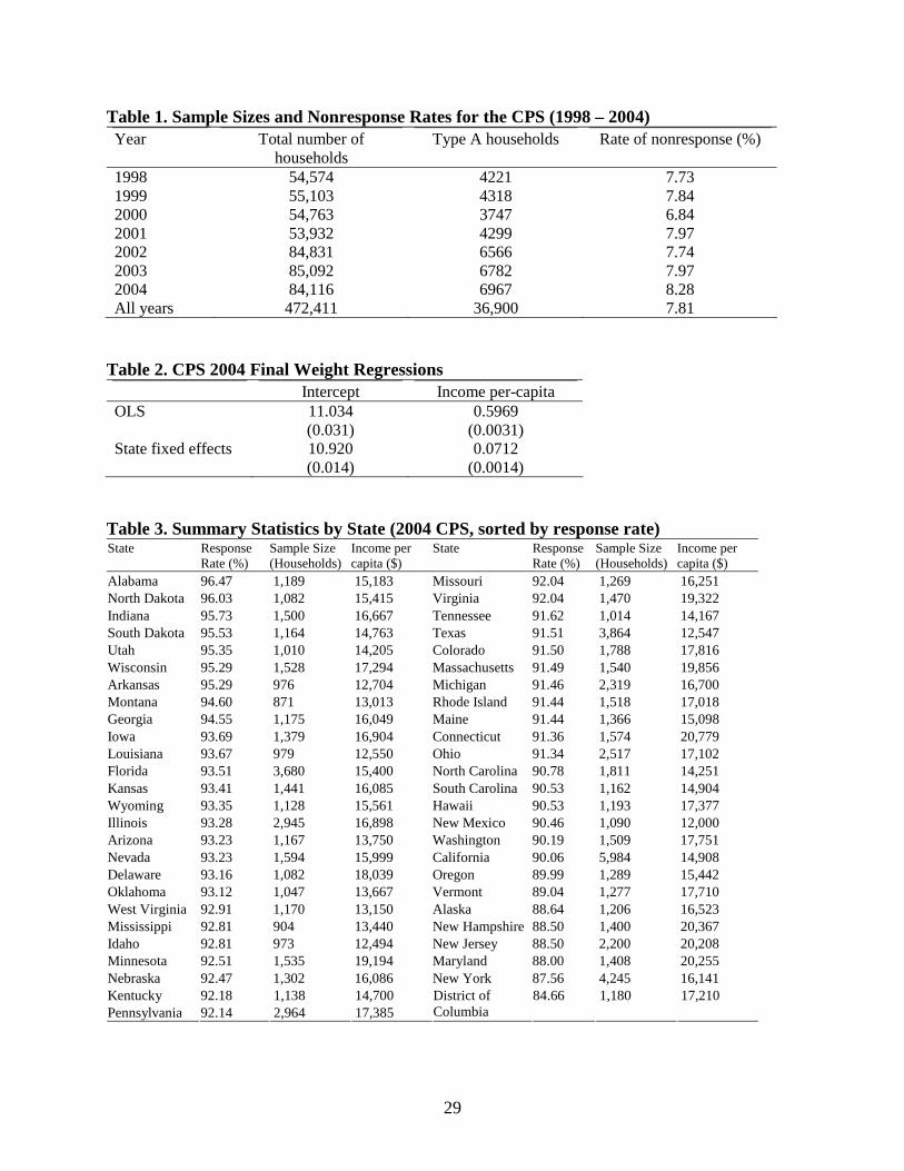
households in the CPS March Supplements from 1998 to 2004 are summarized in Table 1. The

average nonresponse rate is about 8%.

9 The CPS data and survey methodology details are available from the US Census Bureau and can be accessed on-line at: http://www.census.gov/hhes/www/income.html.

12

The CPS adjusts the initial household sampling weights to correct for various factors,

including for nonresponse (described in Census Bureau, 2002, Chapter 10).10 In dealing with

unit nonresponse, the CPS divides all sampled households into 254 adjustment cells. Generally,

these consist of areas within the same metropolitan statistical area (MSA) or an MSA of similar

size and within the same state. MSAs are further split into central and non-central city cells, and

non-MSA areas are split into urban and rural cells.

For each of these adjustment cells, the sampling weight of nonrespondents is re-

distributed to the other households in the cell. In other words, the Census Bureau assumes that

nonresponse is ignorable within adjustment cells. The Census Bureau acknowledges that this

may not be valid and may lead to a nonresponse bias. As we have demonstrated in the previous

section, the described adjustment procedure results in a nonresponse bias.

Ideally we would observe the original CPS sampling weights net of corrections for

nonresponse. Alas, the CPS data sets made available to the public provide only one weight

(called “final weight”) for each household, and that weight reflects various adjustments,

including for nonresponse, sample design, and post-stratification. Thus, since we cannot

disentangle the CPS adjustment for nonresponse from other adjustments, we cannot use the

reported individual CPS household weights in our empirical analysis. Instead, we assign equal

weights to every household within a state. According to the Census Bureau (2002), “most of the

state samples in the CPS come close to being self-weighting,” in other words, “…all units in

[the] sample have the same probability of selection.” This implies that our assumption of equal

household weights within a state will not introduce a bias into our estimations. However, the

10 For a critical assessment of the imputation methods used by the Census Bureau in correcting estimates for income nonresponse see Lillard, Smith and Welch (1986).

13

variance of our state-level inferences will be higher by disregarding these Census Bureau final

weights (i.e., our estimates will be somewhat less efficient).

The March Supplement to the CPS is the source for official national estimates of income

poverty rates and levels in the United Sates as well as the distribution of income (Census Bureau,

2004). Thus, in this application, we will focus on income selected unit nonresponse bias. In

other words, we will determine whether the probability of response of households sampled in the

CPS is a function of their per capita income levels. Using our econometric approach, we then

examine the feasibility of correcting the income distribution for this bias.

Table 2 reports the results of a naïve regression of the reported CPS weights on income,

both with and without State-level fixed effects. We find that there is a significant positive

relationship between per-capita income and the CPS weights, which incorporate the Census

Bureau’s own corrections for nonresponse as well as survey design effects. Thus the Census

Bureau’s correction methodology implicitly acknowledges that their uncorrected survey is biased

towards under-representing higher incomes. The large difference between the OLS and State

fixed effects regression coefficient on income indicates that the bulk of the current CPS

correction is between States rather than within them, though there is still a significant income

effect for the within estimator.

Since the CPS was designed to be representative of the US State level, we can use the 51

States as the geographical areas in our estimation methodology indexed by j. It can be seen from

Table 3 that in 2004, nonresponse rates varied from 3.4% in Alabama to 15.3% in the District of

Columbia.

14

3.1 Specification for the compliance probability as a function of income

To illustrate our estimation approach, we specify the following functional form:

)(

)(

1 i

i

yf

yf

ie

eP

+= (15)

where f(y) is a smooth parametric function and yi is the per-capita income of group i. In our data,

the total number of groups varies between 30,618 in year 2001 and 43,896 in 2003, where a

group comprises all households that report identical per capita income.

Table 4 shows the joint Akaike Information Criterion (AIC) of our minimum distance

estimates for various parametric specifications based on (15) for the years 1998 to 2004. In our

specification tests, we included models with a constant, ln(y), ln(y)2, and y, as well as all possible

combinations of up to three out of the four variables.11 For larger models, the estimated

coefficients tended to be insignificant, since the number of geographic areas in our dataset is not

sufficiently large. Including ln(y)3 or y2 in addition to one of the other variables than the constant

caused problems of multi-collinearity, i.e. the variance-covariance matrix was near singular.

The specification that best fits the nonresponse behavior exhibited by the data, i.e. that

yields the lowest AIC, is specification 3, P = logit[θ1 + θ2 ln(y)], which we thus use in most of

our analysis in the rest of this paper. Since several of the specifications yielded an AIC that was

very close to the -275.37 observed for specification 3, we plot the functional relationship

between compliance and log income for the three best fitting specifications in Figure 1.12 As can

11 In order to apply logarithms to income, we excluded all observations with an income per capita of less than or equal 1 from our sample. In year 2004 for instance, this affected 755 observations. To check whether this changed our results, we also performed an estimation where we used ln(max(y,1)) instead of ln(y) and included all observations. This changed the estimated coefficients in all specifications by less than 2%. 12 The same observation holds if we include all specifications with an AIC below -250 in Table 4. However, the resulting graph becomes very clogged and is thus omitted here.

15

be seen, the resulting curves almost coincide, i.e. using a different specification does not have a

significant effect on our corrections for nonresponse.

The estimated parameters for the different specifications are given in the respective rows

of Table 5. To verify the robustness of our calculated standard errors, we also derived them

numerically using bootstrapping. We randomly sampled 51 states with replacement from the

given set of states and applied our estimator to this sample. After 500 repetitions of this process

we calculated the bootstrapped standard errors as the average squared deviation of the

bootstrapped estimates from the original estimate. For specification 3, they were 3.294 versus the

theoretically derived 1.708 for θ1 and 0.304 versus 0.155 for θ2.

Since the bootstrapped standard errors are almost twice as large, we also performed a

Monte Carlo experiment to determine which set of standard errors is more reliable. We first

estimated the parameter θ and calculated the mean and the standard deviation of log household

income for each of the 51 States. Then we used independent draws from a log normal

distribution with the determined mean and standard deviation to generate a dataset of the size of

the original CPS sample for each State. This constitutes our “base sample.” Next we calculated

for each of the randomly generated households the probability of response according to equation

(15) and performed a Bernoulli experiment with these probabilities to determine whether to

include the household in the “observed” sample, which in turn we used to estimate the parameter

θkMC. After 500 iterations of this process, the standard deviations of the estimated parameters

θkMC had converged to 1.263 and 0.118 for θ1 and θ2 respectively. These are roughly one quarter

lower than the standard errors calculated using equation (11). They are much closer to the

16

theoretically derived standard errors than to the bootstrapped ones. Hence we report the standard

errors according to (11) throughout the paper.13

To investigate the sensitivity of our correction method to the exact choice of

specification, we report estimation results for a number of other specifications, for which the

AIC in Table 4 suggests that they explain the data well. The results can be found in Table 5 (for

the 2004 CPS). Our interest here is whether the different specifications have significantly

different implications for the distribution of income. As can be seen from the Gini coefficient,

the choice of specification does not affect the correction of the distribution significantly: all

corrected Gini coefficients are significantly higher than the uncorrected Gini coefficient of

44.80%, but within one standard deviation of each other, between 49.23% and 49.76%.

It is of interest to see how much the estimated parameters vary over time. Table 6 gives

illustrative results of estimating specification 3 for data from 1998 to 2004, and in the last line

for a dataset that includes all households from 1998 to 2004 (with income chained to 1998 prices

using the regional CPI from the Bureau of Labor Statistics). The parameter estimates of the

individual years are all close to each other, located within a 95% confidence-interval around the

estimate obtained from bundling all years into one data set.

From visual inspection of Table 6, there seems to be no systematic time trend in these

parameters. However, when we tried to verify this proposition by estimating the specification,

13 Further robustness checks using modifications to our Monte Carlo simulations indicated that small changes in the composition of the sample can strongly affect the standard errors that we obtain: An increase in the variability of average household incomes per State, for example, greatly reduces the standard error of our estimator. (This is part of the explanation of why the standard errors from bootstrapping are so large: selecting with replacement from only 51 moment conditions strongly reduces the variability of average household incomes per State.) The described data generating process that we have chosen for our Monte Carlo simulations thus focused on generating a data structure as similar as possible to the observed survey data.

17

P = logit[θ1 + year*θ3 + (θ2 + year*θ4) ln(y)], allowing for a linear time trend in both the

coefficient of income and the constant term, it turned out that both the estimates for θ3 and θ4

were significant. Also, the value of the AIC improves when adding any of the two additional

parameters. The estimation results can be seen at the bottom of Table 9. According to these

parameter estimates, survey response seems to be falling over time since θ3 < 0, but the negative

effect of income on nonresponse seems to be mildly declining, since θ4 > 0.

We tested the sensitivity of our results to making an allowance for geographic cost-of-

living differences, on the presumption that real income should matter more for individuals’

behavior. Ideally we would want to deflate each individual’s income by an indicator of local

consumer prices. Unfortunately, the Bureau of Labor Statistics does not publish data on

consumer prices for the 51 states, but only for four regions (north-east, south, mid-west, and

west) and for metropolitan statistical areas. Furthermore, the published series for these regions

are consumer price indices rather than levels, i.e. they are chained to an average of the prices in

the years 1982-84 of the respective area (rather than to a common denominator), and thus they

only allow comparing prices within a given area over time, but not across areas.

To check sensitivity to this data issue, we used the cost of living indicators of Friar and

Leonard (1998), which are based on a publication of the Bureau of Labor Statistics (1981)

comparing the cost of living of households across different states in that year. Consequently, they

inflated these indicators by the relative increase in the consumer price indices of the metropolitan

statistical areas, which are contained in the respective states, and the respective regional CPI for

rural areas, both of which are published by the Bureau of Labor Statistics. These indicators in

Friar and Leonard (1998) refer to the year 1997. For all following years, we inflate the relative

cost of living measure by the appropriate regional CPI and normalize the indicators so that the

18

average across states is 1.00. The correction of incomes by these relative cost of living indicators

does not significantly affect our estimation results. For a comparison of estimation results for

2004 see Table 7.

We also investigated whether household characteristics other than income have additional

explanatory power for survey compliance. This point is important because omitted variables

might bias our results. Depending on which results we are interested in, we can differentiate

between two kinds of biases. The first refers to the case when we are interested in estimating the

exact functional form of the response function P(Dijξ|Xi, θ). In such a situation, the omission of

any variables that are correlated with both the probability of response and Xi causes a bias in our

estimate of θ. Suppose, for example, that a certain characteristic A is positively correlated with

income and positively correlated with compliance. If A is not included in our estimations, then

our estimate of the effect of income on compliance will be biased upwards (i.e. in absolute terms,

the parameter will be biased downwards). However, the effect of this bias on the income

distribution will be offset to the extent that the variation in A is captured by its correlation with

income, so that we arrive at an unbiased estimate for the corrected income distribution.

The second omitted variable bias is of importance when our object of interest is the

income distribution itself. It arises when we omit a variable that is correlated with the probability

to respond, but uncorrelated to the other variables we include. In this case, our parameter

estimate of θ for the included variables in the function P(Dijξ|Xi, θ) is unbiased, but the corrected

income distribution is biased, since it does not reflect the impact of the omitted variable on

response. In real world applications, it is likely that many omitted variables can be attributed in

part to both of these categories.

19

The additional household characteristics we considered were household size (hhsize), and

dummy variables for whether the interviewed household is located in a metropolitan area (IMSA)

and whether the household owned the house/apartment in which it lived (Ihomeowner). In addition,

we included various characteristics of the household head, such as gender (dummy variable

Ifemale), race (Icaucasian), employment status (dummy variables for Iworking and Iunemployed), education

(measured by an index that indicates the years of schooling, i.e. edu; and alternatively by dummy

variables for attaining different levels of education, of which attaining a graduate degree was

most significant, i.e. Iedu ≥ master), and age, which we use both as a level and squared.

Our results are given in Table 8. The first observation we can make is that the estimated

coefficient on income is highly robust to these changes. We found the included household

characteristics, i.e. household size, metropolitan status and home ownership to be insignificant;

this is also reflected in the AIC for these specifications.

However, there are some characteristics of the household head that should be included

according to the AIC: education, age, and age squared. The impact of the education dummy on

survey nonresponse is strongly negative, but only significant at the 10% level. Since education

and income are positively correlated, it can be expected that the omission of education in our

estimations would bias the estimated coefficient on income upwards. The estimated coefficient

on income in the regression that includes the education dummy is indeed somewhat higher,

though not significantly so.

The effect of age is curious: in a linear specification where only the level of age is

included, our estimate is insignificant and the AIC increases. However, if we include age as well

as age squared in the specification, the coefficient on both becomes significant at the 5% level.

According to our estimates, survey response is high for young people, then it decreases until

20

people reach their mid-50s, after which it increases again. This might be in part explained by

people’s working pattern.

We also estimated a specification that included both age variables and the education

dummy. This yielded an even lower AIC, indicating a better fit with the data. However, our

parameter estimate on income is not significantly changed. Arguably, this could be due to the

low number of geographical areas in our sample, which results in higher standard errors and

therefore a low power for the test of whether the coefficients change.

Another set of variables that we included were regional dummy variables for the Census

Bureau’s four main regions of the US, the North East (1), the Mid-West (2), the South (3) and

the West (4), where we drop the first variable to avoid multi-collinearity. Our estimation results

show that location in the Mid-West significantly increases survey compliance, and the AIC

increases markedly when we add a dummy variable for this region.

Since many of the coefficients in the enhanced specifications of Table 8 yielded the

expected sign but were insignificant, we combined all data from 1998 to 2004 – with income

chained to 1998 prices – in one dataset in order to increase the significance of our results. The

results of our estimations are presented in Table 9.

Among the household variables, household size has a strongly significant negative effect

on survey response. However, the inclusion of household size has little effect on our estimated

coefficient on income. As in our analysis of 2004 data, the dummy variable for metropolitan

areas is insignificant.

There are a large number of characteristics of the household head that have a significant

impact on survey response. According to our estimates, both female and Caucasian household

heads exhibit a lower probability of response than the general population. The same holds for

21

unemployed household heads. Note that as before, the inclusion of these variables does not

significantly affect the parameter estimate for income, even though the standard errors are

smaller now.

With the enlarged dataset, both the estimations using the education index and using the

dummy for graduate studies yield significant parameters. Note that the education dummy also

has a significant effect on the parameter estimate for income now.

3.2 Implications for the empirical distribution of income

The implications for the empirical distribution of income will depend crucially on how

the individual compliance probability varies with income. We saw in Figure 1 that compliance

falls monotonically with income. In Korinek et al., (2005) we study the theoretical implications

of this property for measures of inequality and poverty. Here we summarize the implications for

the empirical distribution of income based on the 2004 CPS.

The effect of correcting for selective compliance on the distribution of income per capita

can be seen from Figures 2 – 4 (again using specification 3 for 2004 data). The uppermost

(dotted) line in Figure 2 shows the uncorrected income distribution, i.e. the observed distribution

if all individuals in a given state are assigned an equal weight, which consists of the population

divided by the size of the sample in the given state. It can be seen that both the corrected CPS

weights and our estimate for a corrected income distribution first order dominate the measured

distribution. For the CPS weights, this dominance seems to be particularly strong for relatively

lower-income households. For our estimation methodology, the correction, and thus the first-

order dominance, is stronger for higher income levels. Consequently, our correction method

assigns comparatively less weight to lower income households and comparatively more weight

22

to higher income households (roughly above an income of $70,000) than the Census Bureau’s

method.

The results indicate that ignoring selective compliance according to income appreciably

understates the proportion of the population in the richest income quantiles and slightly

overstates the population shares in lower quantiles. What is observed as the highest income

percentile in the survey, for example, is estimated to comprise 2.21% (+/– 0.47%) of the

population after correcting for its lower probability of survey compliance, and the highest

observed decile actually makes up for 12.95% (+/– 0.61%) of the population. By contrast, the

poorest observed decile and percentile in the unadjusted data actually comprise only 9.34% (+/–

0.04%) and 0.93% (+/–0.01%) respectively of the corrected population. The correction method

of the Census Bureau, by contrast, assigns 1.60% and 15.74% of the population weight

respectively to the top observed percentile and decile, and 6.95% and 0.88% to the bottom decile

and percentile.

Using our correction method, median income per person rises from an uncorrected

$16,096 to $17,085, while the mean increases from an uncorrected $22,039 to $25,735 per

capita. Using the weights provided by the Census Bureau, median income rises to $19,333, and

mean income to $26,958.

Figure 3 shows a magnification of the lower 25% of the distribution. It can be seen that

using our correction method, the impact on poverty incidence is small for poverty lines

commonly used in the U.S., giving poverty rates around 12% (Census Bureau, 2001). However,

since there is first-order dominance, poverty measures using the uncorrected, equally-weighted

distribution of incomes unambiguously overestimate poverty. Note that the correction

23

methodology of the Census Bureau leads to a significant underestimation in the estimated level

of poverty according to our results.

Figure 4 depicts the Lorenz curves for the uncorrected income distribution, the

distribution according to the Census Bureau’s weights, and according to our correction method.

The effect of our correction for selective response is a marked downward shift in the Lorenz

curve, implying higher inequality. However, there is not strict Lorenz dominance, with an

intersection of the Lorenz curves for the corrected and uncorrected distributions occurring at the

extreme upper end of the income range. Korinek et al., (2005) show that this intersection is a

theoretical implication of a monotonic income effect on compliance.

By inverting the CDF to obtain the quantile function for the original distribution we can

calculate the income correction at each percentile of income that was observed in the raw survey.

We do this for the correction implied by the Census Bureau weights, and the corrected

distribution according to our method. The results are given in Figure 5. For the Census Bureau’s

correction, income at any given percentile shifts up almost uniformly by about 20%. This implies

that the Census Bureau’s correction method affects the national average, but is almost

distribution neutral. For our method, the correction is quite low (around +2 to +3%) for the

bottom 9 deciles and then rises sharply, to reach almost +100% for the uppermost percentile.

Figure 6 depicts the weight correction of each observed income percentile. This figure

reveals why the Census Bureau’s correction method has almost no effect on inequality: their

methodology heavily reduces the weights of low-income individuals (by almost 40% for some of

the bottom percentiles) and attributes this weight to the uppermost third of the income

distribution. Our method, in contrast, reduces the weight of bottom four-fifth only by roughly

3%, and redistributes this weight to the top percentiles.

24

The above results have been based on one specification of the compliance probability

model, specification 3. In Korinek at el., (2005) we also report results for measures of inequality

for the various alternative specifications discussed in section 3.1 and we show that the measures

obtained are quite robust to the changes in model specification.

4. Conclusions

Past empirical work has either ignored the problem of selective compliance in surveys or

made essentially ad hoc corrections. We have shown how the latent income effect on compliance

can be estimated consistently with the available data on average response rates and the measured

distribution of income across geographic areas. Thus we are able to re-weight the raw data to

correct for the problem. In an example using US data, we find that we can reject the assumptions

made in past ad hoc correction methods. A highly significant negative income effect on survey

compliance is indicated by our results. Our method also indicates higher inequality than implied

by the survey’s internal weights. An upward revision to the overall mean is also called for to

correct for selective compliance.

Ideally, the adjustment methods employed by the Census Bureau to correct for various

sampling errors as well as the post-stratification methods could be combined with our correction

method for nonresponse to obtain the most efficient estimate of population statistics possible and

to balance off the biases that are introduced by the various methods. Technically, this would be

no problem. However, the CPS dataset did not provide us with the sample weights before

correction for nonresponse or the detailed data used for post-stratification, which would both be

required for such a calculation. We thus recommend to the Census Bureau to include sample

weights that are unadjusted for non-response in future data releases.

25

There can be no presumption that our quantitative results will hold elsewhere. Possibly

in poorer settings one will find greater under-representation of the poor than in the US. Or one

might find a less (more) steep income gradient of compliance in countries with lower (higher)

inequality than the US. These are conjectures. However, the data and computational demands of

the method we have proposed are quite modest, so other applications can easily be implemented.

26

Appendix

The proof of the Proposition in Section 2 is as follows. Let {Sj}j = 1…J be J samples of

households that can be partitioned into I subsets with characteristics Xi each. Suppose without

loss of generality that ∑i mij = mj = 1, and that the probability of response P(Dijξ = 1|Xi, θ) is

strictly increasing in Xi. Then let us show that for any geographical subgroup j, the observed

average 1jX is in expectation lower than the actual (but unobserved) average ∑ =

= I

i ijij mXX1

.

To prove this we establish that the contrary yields a contradiction. Suppose that:

∑∑∑

==

= ≥= Ii ijiI

i iji

Ii ijii

j mXmP

mPXXE 1

1

11 ][

This can be transformed into:

01

1

≥

−∑

∑==

Ii ijI

i iji

ijii m

mP

mPX

Note that we can rewrite PmPI

i iji =∑ =1, since it represents an average probability of response.

Now observe that, since Pi(⋅|Xi) is strictly increasing in Xi, there must be some X~

such that

( ) XXPXP iii

~, ≥∀≤⋅ and ( ) XXPXP iii

~, ≥∀≥⋅ . We can use this to restate the

equation above as:

( ) 0~

1

≥

−−∑

=

I

iij

ijii m

P

mPXX or ( ) 01

~

1

≥

−−∑

=

I

i

iiji P

PmXX

It is straightforward to see that all addends on the left hand side are zero or negative; for XX i

~≥

the term in the first parentheses is positive or zero and the one in the second parentheses is

negative or zero. For XX i

~< , the term in the first parentheses is negative and the one in the

second parentheses positive. Thus we have a contradiction and it must be the case that

jj XXE <][ 1 . Having shown that the observed average 1jX is in expectation below the actual

average jX for every single area j, the claim in the proposition follows readily by averaging

over all J areas.

27

References

Bureau of Labor Statistics, 1981, Urban family budgets and comparative indexes for selected

urban areas. U.S. Department of Labor, Washington DC.

Cassel, C-M., Sarndal, C-E., Wretman, J.H., 1983, Some uses of statistical models in connection

with the nonresponse problem, in: Madow, W.G. Olkin, I. (Eds.), Incomplete Data in

Sample Surveys, Vol. 3. Academic, New York.

Census Bureau, 2001, Poverty in the United States: 2001. Current Population Report P60-219.

U.S. Department of Commerce, Washington, DC.

Census Bureau, 2002, Current Population Survey: Design and Methodology. Technical Paper

63RV. U.S. Department of Commerce, Washington DC.

Census Bureau, 2004, Income, poverty, and health insurance coverage in the United States.

Current Population Report P60-226. U.S. Department of Commerce, Washington DC.

Chapman, D.W., 1983, The impact of substitution on survey estimates. In: Madow, W.G. Olkin,

I. (Eds.), Incomplete Data in Sample Surveys, Vol. 2. Academic Press, New York.

Deming, W.E., 1953, On a probability mechanism to attain an economic balance between the

resultant error of response and the bias of nonresponse. Journal of the American

Statistical Association 48, 743-772.

Friar, M.E., Leonard, H.B. 1998. Variations in cost of living across States. Taubman Center for

State and Local Government, John F. Kennedy School, Harvard University.

Gannon, M.J., Nothern, J.C., Carroll, S.J., 1971, Characteristics of nonrespondents among

workers. Journal of Applied Psychology 55, 586-588.

Groves, R.E., Couper, M.P., 1998, Nonresponse in Household Interview Surveys. Wiley, New

York.

Hansen, L.P., 1982, Large sample properties of Generalized Method of Moments estimators.

Econometrica 50, 1029-1054.

Hansen, M.H., Hurwitz, W.N., Madow, W.G., 1953, Sample survey methods and theory, Vol. 1.

Wiley, New York.

Hansen, M.H., Hurwitz, W.N. 1946, The problem of nonresponse in sample surveys. Journal of

the American Statistical Association 41, 516-529.

28

Hendricks, W.A., 1949, Adjustment for bias caused by nonresponse in mailed surveys.

Agricultural Economic Research 1, 52-56.

Holt, D., Elliot, D., 1991, Methods of Weighting for Unit Nonresponse. The Statistician 40, 333-

342.

Kalsbeek, W.D., Folsom Jr., R.E., Clemmer, A.F., 1974, The national assessment no-show

study : an examination of nonresponse bias. American Statistical Association

Proceedings of the Social Statistics Section, 180-189.

Kalton, G., Kasprzyk, D., 1982, Imputing for missing survey response. American Statistical

Association Proceedings of the Survey Research Methods Section, 21-33.

Korinek, A., Mistiaen, J.A., Ravallion, M., 2005, Survey Nonresponse and the Distribution of

Income, forthcoming in Journal of Economic Inequality.

Lessler, J.T., Kalsbeek W. D., 1992, Nonsampling Error in Surveys. Wiley, New York.

Lillard, L., Smith, J.P., Welch F., 1986. What Do We Really Know about Wages? The

Importance of Nonreporting and Census Imputation. Journal of Political Economy 94,

489-506.

Little, R.J.A., Rubin D.B., 1987, Statistical Analysis with Missing Data. Wiley, New York.

Moser, C.A., Kalton, G., 1972, Survey Methods in Social Investigation. Basic Books, New York.

Philipson, T., 1997. Data markets and the production of surveys. Review of Economic Studies

64, 47-72.

Politz, A.N., Simmons, W.R., 1949, An attempt to get ‘not-at-homes’ into the sample without

call-backs. Journal of the American Statistical Association 44, 9-31.

Rubin, D.B., 1977, Formalizing subjective notions about the effects of nonrespondents in sample

surveys. Journal of the American Statistical Association 72, 538-543.

Scott, K., Steele, D., 2004, Measuring Welfare in Developing Countries: Living Standards

Measurement Study Surveys. In: Surveys in Developing and Transition Countries:

Design, Implementation and Analysis. United Nations, New York.

Thomsen, I., 1973, A note on the efficiency of weighting subclass means to reduce effects of

non-response when analyzing survey data. Statistisk Tidskrift 4, 278-283.

29

Table 1. Sample Sizes and Nonresponse Rates for the CPS (1998 – 2004) Year Total number of

households Type A households Rate of nonresponse (%)

1998 54,574 4221 7.73 1999 55,103 4318 7.84 2000 54,763 3747 6.84 2001 53,932 4299 7.97 2002 84,831 6566 7.74 2003 85,092 6782 7.97 2004 84,116 6967 8.28 All years 472,411 36,900 7.81

Table 2. CPS 2004 Final Weight Regressions Intercept Income per-capita OLS 11.034 0.5969 (0.031) (0.0031) State fixed effects 10.920 0.0712 (0.014) (0.0014)

Table 3. Summary Statistics by State (2004 CPS, sorted by response rate) State Response

Rate (%) Sample Size (Households)

Income per capita ($)

State Response Rate (%)

Sample Size (Households)

Income per capita ($)

Alabama 96.47 1,189 15,183 Missouri 92.04 1,269 16,251 North Dakota 96.03 1,082 15,415 Virginia 92.04 1,470 19,322 Indiana 95.73 1,500 16,667 Tennessee 91.62 1,014 14,167 South Dakota 95.53 1,164 14,763 Texas 91.51 3,864 12,547 Utah 95.35 1,010 14,205 Colorado 91.50 1,788 17,816 Wisconsin 95.29 1,528 17,294 Massachusetts 91.49 1,540 19,856 Arkansas 95.29 976 12,704 Michigan 91.46 2,319 16,700 Montana 94.60 871 13,013 Rhode Island 91.44 1,518 17,018 Georgia 94.55 1,175 16,049 Maine 91.44 1,366 15,098 Iowa 93.69 1,379 16,904 Connecticut 91.36 1,574 20,779 Louisiana 93.67 979 12,550 Ohio 91.34 2,517 17,102 Florida 93.51 3,680 15,400 North Carolina 90.78 1,811 14,251 Kansas 93.41 1,441 16,085 South Carolina 90.53 1,162 14,904 Wyoming 93.35 1,128 15,561 Hawaii 90.53 1,193 17,377 Illinois 93.28 2,945 16,898 New Mexico 90.46 1,090 12,000 Arizona 93.23 1,167 13,750 Washington 90.19 1,509 17,751 Nevada 93.23 1,594 15,999 California 90.06 5,984 14,908 Delaware 93.16 1,082 18,039 Oregon 89.99 1,289 15,442 Oklahoma 93.12 1,047 13,667 Vermont 89.04 1,277 17,710 West Virginia 92.91 1,170 13,150 Alaska 88.64 1,206 16,523 Mississippi 92.81 904 13,440 New Hampshire 88.50 1,400 20,367 Idaho 92.81 973 12,494 New Jersey 88.50 2,200 20,208 Minnesota 92.51 1,535 19,194 Maryland 88.00 1,408 20,255 Nebraska 92.47 1,302 16,086 New York 87.56 4,245 16,141 Kentucky 92.18 1,138 14,700 84.66 1,180 17,210 Pennsylvania 92.14 2,964 17,385

District of Columbia

30

Table 4. AIC for various specifications, 1998 – 2004 data Specification AIC

1: zi = θ1 -69.27

2: zi = θ1 ln(yi) -42.20

3: zi = θ1 + θ2 ln(yi) -276.14 4: zi = θ1 ln(yi)

2 -16.04

5: zi = θ1 + θ2 ln(yi)2 -275.37

6: zi = θ1 ln(yi) + θ2 ln(yi)2 -273.45

7: zi = θ1 + θ2 ln(yi) + θ3 ln(yi)2 -270.04

8: zi = θ1 yi 88.78

9: zi = θ1 + θ2 yi -193.05

10: zi = θ1 ln(yi) + θ2 yi -159.03

11: zi = θ1 + θ2 ln(yi) + θ3 yi -273.04

12: zi = θ1 ln(yi)2+ θ2 yi -119.01

13: zi = θ1 + θ2 ln(yi)2 + θ3 yi -273.31

14: zi = θ1 ln(yi) + θ2 ln(yi)2 + θ3 yi -273.77

Note: The probability of response is modeled as P = logit(z) for all given models. In order to determine the Akaike Information Coefficient (AIC) for the various specifications, we estimated each specification with data from all 7 years and used the resulting residuals ψj to

calculate ( )( ) mJJAIC j 2ˆlog 2 +⋅= ∑ θψ , where J is the number of residuals, i.e. 7*51 here, and m is

the number of estimated parameters, i.e. 7, 14 or 21 in our application. The lowest value for the AIC (i.e. here the highest absolute value) indicates that specification 3 (underlined in the table above) best fits the nonresponse behavior exhibited by our data. For our estimations we are using Matlab 6.5. The source code of our program can be downloaded at http://econ.worldbank.org/programs/poverty/topic/2678/

31

Table 5. Various Specifications for 2004 CPS

Specification θ1 θ2 θ3 Gini index (%)

3: z = θ1 + θ2 ln(y) 19.112 (1.708)

-1.613 (0.155)

49.23 (0.92)

5: z = θ1 + θ2 ln(y)2 10.108 (0.747)

-0.07165 (0.00611)

49.41 (0.90)

6: z = θ1 ln(y) + θ2 ln(y)2 1.8091

(0.1165) -0.1519

(0.0105)

49.60 (0.87)

7: z = θ1 + θ2 ln(y) + θ3 ln(y)2 -1.1568

(9.7906) 2.017

(1.766) -0.1611

(0.0791) 49.63 (0.93)

9: z = θ1 + θ2 y 2.900

(0.055) -1.232*10-5

(4.368*10-7)

49.56 (0.62)

11: z = θ1 + θ2 ln(y) + θ3 y 7.968

(3.878) -0.5113

(0.3865) -8.704*10-6

(2.755*10-6) 49.62 (0.69)

13: z = θ1 + θ2 ln(y)2 + θ3 y 5.396

(1.896) -0.02541

(0.01885) -8.221*10-6

(3.072*10-6) 49.66 (0.69)

14: z = θ1 ln(y) + θ2 ln(y)2 + θ3 y 1.0752

(0.3615) -0.07891

(0.03610) -7.199*10-6

(3.328*10-6) 49.76 (0.70)

Note: Standard errors are in brackets. The uncorrected Gini coefficient for 2004 data (with households equally weighted within states) is 44.80%, and using the official CPS weights it is 45.20%. Table 6. Specification P = logit[θ1 + θ2 ln(y)] – Estimates for 1998 – 2004

1998 1999 2000 2001 2002 2003 2004 All

θ1 19.904 (2.071)

18.100 (2.420)

22.207 (2.545)

20.111 (1.728)

17.807 (1.920)

17.388 (2.100)

19.113 (1.708)

18.838 (0.793)

θ2 -1.696

(0.188) -1.528 (0.223)

-1.890 (0.230)

-1.702 (0.156)

-1.490 (0.176)

-1.454 (0.193)

-1.613 (0.155)

-1.599 (0.073)

Note: standard errors in brackets Table 7. Specification P = logit[θ1 + θ2 ln(y)] using cost-of-living adjustment for 2004 data

Income y in nominal terms Income y in real terms

θ1 19.113 (1.708)

18.337 (2.501)

θ2 -1.613 (0.155)

-1.542 (0.229)

Note: standard errors in brackets

32

Table 8. Augmented specifications for 2004 data Specification θ1 θ2 θ3 θ4 θ5 AIC

zi = θ1 + θ2 ln(yi) [baseline] 19.113 (1.708)

-1.613 (0.155)

-23.881

zi = θ1 + θ2 ln(yi) + θ3 hhsize 18.092 (2.545)

-1.545 (0.197)

0.1315 (0.2623)

-22.205

zi = θ1 + θ2 ln(yi) + θ3 IMSA 20.010 (1.896)

-1.705 (0.178)

0.1462 (0.1790)

-22.568

zi = θ1 + θ2 ln(yi) + θ3 Ihomeowner 18.436 (1.571)

-1.648 (0.151)

1.107 (0.678)

-23.271

zi = θ1 + θ2 ln(yi) + θ3 Ifemale 18.804 (1.808)

-1.569 (0.18)

-0.3703 (0.7412)

-22.204

zi = θ1 + θ2 ln(yi) + θ3 Icaucasian 17.669 (2.290)

-1.499 (0.199)

0.2607 (0.2799)

-22.689

zi = θ1 + θ2 ln(yi) + θ3 Iworking 19.143 (1.715)

-1.612 (0.172)

-0.0455 (1.2631)

-21.883

zi = θ1 + θ2 ln(yi) + θ3 Iunemployed 18.709 (1.766)

-1.57 (0.163)

-1.4699 (1.3966)

-22.241

zi = θ1 + θ2 ln(yi) + θ3 edu 17.304 (2.38)

-1.183 (0.437)

-0.2567 (0.2456)

-23.231

zi = θ1 + θ2 ln(yi) + θ3 Iedu ≥ master 11.347 (4.51)

-0.821 (0.479)

-1.9618 (1.1183)

-26.625

zi = θ1 + θ2 ln(yi) + θ3 age 19.866 (2.327)

-1.629 (0.162)

-0.0114 (0.0221)

-22.345

zi = θ1 + θ2 ln(yi) + θ3 age + + θ4 age2

127.215 (50.518)

-1.784 (0.138)

-3.934 (1.850)

0.03596 (0.01671)

-36.922

zi = θ1 + θ2 ln(yi) + θ3 age + + θ4 age2 + θ5 Iedu ≥ master

97.365 (44.926)

-1.572 (0.215)

-2.909 (1.661)

0.02653 (0.01500)

-0.6948 (0.3835)

-38.500

zi = θ1 + θ2 ln(yi) + θ3 Iregion 2 + + θ4 Iregion 3 + θ5 Iregion 4

16.991 (1.794)

-1.428 (0.164)

0.2762 (0.1012)

0.1020 (0.0809)

0.0744 (0.0816)

-26.122

zi = θ1 + θ2 ln(yi) + θ3 Iregion 2 17.319 (1.813)

-1.453 (0.166)

0.2126 (0.0935)

-28.219

Note: standard errors in brackets

33

Table 9. Augmented specifications for pooled data from 1998 to 2004 Specification θ1 θ2 θ3 θ4 AIC

zi = θ1 + θ2 ln(yi) [baseline] 18.838 (0.793)

-1.599 (0.073)

-262.51

zi = θ1 + θ2 ln(yi)+ θ3 hhsize 21.383 (1.022)

-1.759 (0.085)

-0.342 (0.068)

-275.65

zi = θ1 + θ2 ln(yi)+ θ3 IMSA 18.892 (0.925)

-1.605 (0.089)

0.010 (0.092)

-260.52

zi = θ1 + θ2 ln(yi)+ θ3 Ifemale 18.383 (0.813)

-1.521 (0.080)

-0.812 (0.308)

-270.74

zi = θ1 + θ2 ln(yi)+ θ3 Icaucasian 19.004 (0.776)

-1.611 (0.071)

-0.116 (0.038)

-273.01

zi = θ1 + θ2 ln(yi)+ θ3 Iworking 18.808 (0.802)

-1.617 (0.082)

0.281 (0.411)

-261.14

zi = θ1 + θ2 ln(yi)+ θ3 Iunemployed 18.472 (0.807)

-1.561 (0.075)

-1.336 (0.438)

-264.78

zi = θ1 + θ2 ln(yi)+ θ3 edu 16.587 (1.041)

-1.162 (0.167)

-0.223 (0.085)

-271.22

zi = θ1 + θ2 ln(yi)+ θ3 Iedu ≥ master 15.482 (1.434)

-1.231 (0.158)

-1.020 (0.445)

-269.95

zi = θ1 + θ2 ln(yi)+ θ3 age 19.274 (1.065)

-1.614 (0.076)

-0.006 (0.009)

-261.04

zi = θ1 + θ2 ln(yi)+ θ3 age + θ4 age2 20.180 (2.302)

-1.607 (0.077)

-0.045 (0.081)

0.0004 (0.0007)

-259.47

zi = θ1 + θ2 ln(yi)+ θ3 year 18.858 (0.785)

-1.595 (0.072)

-0.020 (0.008)

-269.98

zi = θ1 + year*θ3 + [θ2 + year*θ4] ln(yi) 22.179 (1.293)

-1.898 (0.117)

-0.948 (0.310)

0.0849 (0.0283)

-273.42

Note: standard errors in brackets

34

Figure 1: Probability of response function, top three specifications, 1998 – 2004 data

$1000 $2000 $4000 $10,000 $20,000 $40,000 $100,0000.5

0.55

0.6

0.65

0.7

0.75

0.8

0.85

0.9

0.95

1

Y ... income/capita

prob

abili

ty o

f co

mpl

ianc

e

bottom percentiletop percentilespecification 3specification 5specification 14

Note: The graphs of the three specifications of nonresponse that match the data most closely almost coincide, indicating that the exact choice of specification is not of major importance. 95% confidence intervals were computed, but are visibly almost indistinguishable from the graphed functions themselves and were thus omitted. The two dotted vertical lines indicate the interval in which the median 98% of income observations are located.

35

Figure 2: Empirical and compliance corrected cumulative income distribution

$0 $50,000 $100,000 $150,0000

0.1

0.2

0.3

0.4

0.5

0.6

0.7

0.8

0.9

1Corrected income distribution for 2004 data

frac

tion

of p

opul

atio

n

income per capita

uncorrectedCPS weightscorrected

Note: The upper (dotted) line represents the income distribution from raw survey data without the Census Bureau’s weight adjustments. The dash-dot line depicts the income distribution using the adjustment weights of the Census Bureau. Finally, the solid line shows the distribution according to our correction method. A 95% confidence interval for our corrected distribution line was computed but is omitted here, since it was visibly almost indistinguishable from the line itself.

36

Figure 3: Lower segment of cumulative income distribution from Figure 2

$0 $2,000 $4,000 $6,000 $8,000 $10,0000

0.05

0.1

0.15

0.2

0.25Corrected income distribution for 2004 data

frac

tion

of p

opul

atio

n

income per capita

uncorrectedCPS weightscorrected

Note: The figure gives a magnification of the lower part of the cumulative income distribution reveals that our correction method assigns comparatively less weight to lower income households than the Census Bureau’s correction method.

37

Figure 4: Observed and corrected Lorenz curves

0 0.2 0.4 0.6 0.8 10

0.1

0.2

0.3

0.4

0.5

0.6

0.7

0.8

0.9

1Lorenz curves for 2004 data

frac

tion

of t

otal

inco

me

fraction of population

uncorrectedCPS weightscorrected

Note: The top line (dotted) shows the Lorenz curve using un-weighted data, the second (dash-dot) line is the Lorenz curve using the weights provided by the Census Bureau. This line hardly differs from the un-weighted data. The bottom (solid) line is the Lorenz curve according to our correction for survey nonresponse: it shows a marked increase in inequality as compared to the previous two cases. We also calculated a 99% confidence interval for our correction method. However, since this visibly almost coincides with the depicted line, it was omitted in the given graph.

38

Figure 5: Percentage correction of income by percentile of income distribution

0% 10% 20% 30% 40% 50% 60% 70% 80% 90% 100%

-10%

0%

+10%

+20%

+30%

+40%

+50%Implied income correction for 2004

impl

ied

inco

me

corr

ectio

n

percentile of income

Our correctionCPS correctionBaseline

Note: The figure shows by how much the income of a given income percentile in the corrected distribution is revised with respect to the income of the same percentile in the equally weighted income distribution. The Census Bureau’s method implies a relatively uniform shift of incomes in each percentile by roughly 20% upwards. Our correction method shifts the income of lower income percentiles only modestly upwards, whereas the mean income of the top percentile is corrected by almost 40%.

39

Figure 6: Weight correction for each observed percentile

0% 10% 20% 30% 40% 50% 60% 70% 80% 90% 100%-40%

-20%

0%

+20%

+40%

+60%

+80%

+100%Weight correction for 2004

impl

ied

wei

ght

corr

ectio

n fo

r ob

serv

ed p

erce

ntile

percentile of income

Our correctionCPS correctionBaseline

Note: The figure presents the data from the previous graph in a different format: Instead of comparing percentiles in the un-weighted distribution with percentiles in the corrected distribution, we depict the correction in the sum of weights of all households contained in a given percentile of the un-weighted income distribution. As can be seen, the Census Bureau’s method strongly reduces the weights of the lower income percentiles in the un-weighted distribution and increases the weights of the upper third of the observed income distribution. Our correction method slightly decreases the weights of all households below the 83rd percentile and strongly increases the weights of the households in the top observed percentiles.