9. Microwaves

MW

9.1 Introduction

Electromagnetic waves with wavelengths of the order of 1 mm to 1 m, or equivalently, with fre-

quencies from 0.3 GHz to 0.3 THz, are commonly known as microwaves, sometimes also centimetre

waves.1 The characterising name for these waves is motivated purely by technological reasons; the

physics is the same for all electromagnetic waves, and the same fundamental theoretical relations

apply, the Maxwell equations.

Microwaves are of great technical importance for many different applications, such as radar, com-

munication links (satellite and earthbound transponders), as carrier waves for cellular telephone

transmission, used in heating equipment (laboratory and kitchen) to name but a few. Common

sources of microwaves use either vacuum tube technology (e.g. a klystron), or solid-state technol-

ogy, microwave diodes, as in this lab, where the active element is a Gunn diode. The wave may be

continuous, or consist of short repeated bursts of energy.

Just as for the visible range of the electromagnetic spectrum (light) (cf. labs I, M, Spm), microwaves

are subject to reflection, absorption, polarization, scattering, diffraction, and interference.

In the present three-part laboratory, absorption and reflection of microwaves will be investigated,

the wavelength of the microwave source determined using a Michelson interferometer, and the

diffraction and interference patterns for single and double slits measured.

Safety consideration

Although the transmitted radiation is of low power, do not expose your head and eyes to the

radiation, in particular not close to the opening of the transmitter horn. Remember that metallic

surfaces reflects almost perfectly microwave radiation. Never remove the horn wave-guide from the

transmitter whilst connected to the power supply. Do not connect the receiver to a voltage supply;

the terminals are intended for an audio amplifier.

1Microwaves are also defined as the waves in the frequency range for which the electronic circuitry is not designed

with coils and condensers, but with wave-guide and transmission line technology. The upper frequency limit also

marks the onset of atmospheric absorption.

1

2 9. Microwaves

9.2 Theory

a) Electromagnetic waves

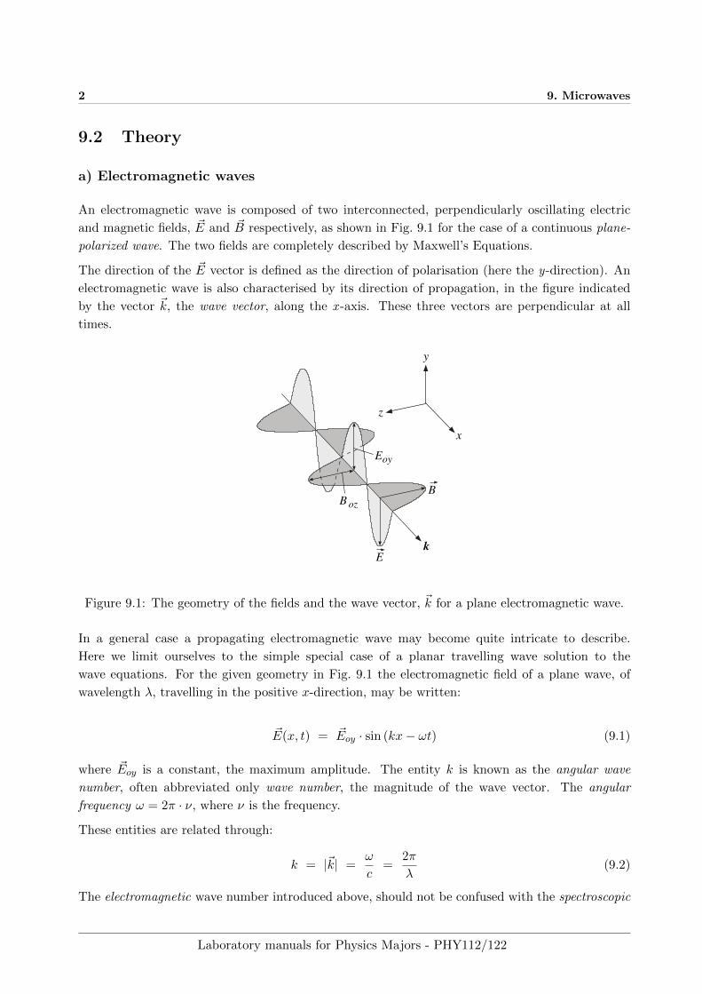
An electromagnetic wave is composed of two interconnected, perpendicularly oscillating electric

and magnetic fields, ~E and ~B respectively, as shown in Fig. 9.1 for the case of a continuous plane-

polarized wave. The two fields are completely described by Maxwell’s Equations.

The direction of the ~E vector is defined as the direction of polarisation (here the y-direction). An

electromagnetic wave is also characterised by its direction of propagation, in the figure indicated

by the vector ~k, the wave vector, along the x -axis. These three vectors are perpendicular at all

times.

y

z

x

Eoy

B ozB

Ek

Figure 9.1: The geometry of the fields and the wave vector, ~k for a plane electromagnetic wave.

In a general case a propagating electromagnetic wave may become quite intricate to describe.

Here we limit ourselves to the simple special case of a planar travelling wave solution to the

wave equations. For the given geometry in Fig. 9.1 the electromagnetic field of a plane wave, of

wavelength λ, travelling in the positive x-direction, may be written:

~E(x, t) = ~Eoy · sin (kx− ωt) (9.1)

where ~Eoy is a constant, the maximum amplitude. The entity k is known as the angular wave

number, often abbreviated only wave number, the magnitude of the wave vector. The angular

frequency ω = 2π · ν, where ν is the frequency.

These entities are related through:

k = |~k| =ω

c=

2π

λ(9.2)

The electromagnetic wave number introduced above, should not be confused with the spectroscopic

Laboratory manuals for Physics Majors - PHY112/122

9.2. THEORY 3

wave number2 ν̃ = 1/λ, as used in atomic physics, and sometimes also designated k.

Linear polarisation (or plane polarisation) requires that the ~E-field vector is always oscillating in

the same plane.

The intensity I of any wave is defined as the energy transmitted through a surface perpendicular to

the direction of propagation (the wave vector). For an electromagnetic wave this is the time average

of the product of the magnitude of the two fields. According to Maxwell’s equations B ∝ E, which

is equivalent to saying that the intensity is proportional to the time average of the square of the

strength of the electric field. We write this as:

I ∝ E2(t) (9.3)

b) Diffraction and Interference

The theory of wave diffraction in a single slit and wave interference in a double slit is thoroughly

treated in the theory section of the manual for lab I. Only the main results will be briefly summarised

in the following. One should recall here that the phenomena of diffraction and interference appear

at openings and slits with dimensions that are of the order of the wavelength of the radiation.

Single slit diffraction

A wave with wavelength λ, perpendicularly incident on a single slit of width s, gives rise to a

diffraction pattern far behind the slit, (Fraunhofer diffraction), e.g. on a distant screen, with

minima (dark straight fringes parallel to the slit) at angles θ determined by the relation:

sin θ = n · λs

where the integer n = ±1,±2,±3 . . . (9.4)

Angle θ is measured from the normal of the plane containing the slit. The respective minima are

said to be of order n.

For a perpendicularly incident wave, single slit diffraction intensity maxima is found at angles

approximately described by the relation:

sin θ = (n+1

2) · λs

where n = 0,±1,±2,±3 . . . (9.5)

This is a nontrivial result.

It is worth noting, that the angles for both maxima and minima depends inversely on the the slit

width, so that the essential features of the pattern becomes larger for decreasing slit width.

As shown in the right part of Fig. 9.2 the intensity of the maxima decreases strongly with angle.

The ordinate shows the square root of the intensity I only for the sake of convenience.

2By tradition the spectroscopic wave number is sometimes given in units of reciprocal centimeters, cm−1 or keyser

(sometimes even retemitnec),

Laboratory manuals for Physics Majors - PHY112/122

4 9. Microwaves

Double slit diffraction (Young’s experiment)

The electrically generated microwaves have good spatial coherence, and therefore the wave incident

on a double slit will give rise to interfering waves. The intensity variation is determined by inter-

ference between waves from the two slits, and diffraction in each of the two single slits. With slit

centre distance d, a perpendicularly incident wave with wavelength λ, gives rise to a complicated

intensity variation. Minima, i.e. dark fringes parallel to the slits, appear at angles θ, determined

by the relation:

sin θ = (n+1

2) · λd

where n = 1, 2, 3, . . . (9.6)

Intensity maxima occur at angles θ according to the relation:

sin θ = n · λd

with n = 1, 2, 3, . . . (9.7)

These results are obtained straightforwardly, but they only describe the angular positions of minima

and maxima. The full expressions for the intensity variations are quite a bit more complicated. For

the hypothetical case of infinitely narrow slits (there would actually be no intensity) the maxima

would all be equally intense. The square root of the intensity distribution for the double slit with

finite slit widths is shown on the right in Fig. 9.2, showing the intensity of single slit diffraction as

an envelope to the double slit interference intensity maxima.

θ

θ

sin

sin

I

I ( )e

θsin

I

-2 -1 0 1 2 (λ/s)

Figure 9.2: Intensity distribution for diffraction in a single slit (left) and a double slit (right).

c) The Michelson interferometer

The Michelson interferometer is treated in some detail in the theory section of the manual for lab

M, and in this manual section 9.3. Although different in mechanical design, the principles of the

set-up employed here are the same, and therefore only the main features are summarised. Compare

Fig. 9.5 and the corresponding figure in lab M.

Superposition of coherent waves may cause phenomena related to interference. Assuming sufficient

coherence, we restrict ourselves here to the case of two interfering waves from a single source.

Depending on the relative phase of the waves, their electromagnetic fields may add constructively

or destructively, thus creating an interference pattern. Since the wavelength for microwaves is about

Laboratory manuals for Physics Majors - PHY112/122

9.2. THEORY 5

five orders of magnitude larger than for visible light, the features of the pattern will be accordingly

larger.

The interferometer is designed for investigation of interfering waves from a single source. The

beam is split in two perpendicular paths by a partially reflecting mirror (beam splitter), which for

microwaves may be a wire grating, as in the present lab. The interferometer arms are implemented

as short optical benches for sliding or fastening the two perpendicularly mounted aluminium sheet

metal screens acting as mirrors at the end of each path. The beams are reflected back onto the beam

splitter, and brought to interfere such that a pattern of interference results. As opposed to the case

of the Michelson interferometer for visible light, cf. lab M, there is no extra half wavelength path

difference here because of the beam splitter, and therefore the condition for destructive interference

(a dark fringe) on the optical axis (at the centre of the pattern), requires the optical path difference

∆W0 of the two beams to be:

∆W0 = (n+1

2) · λ with n = 0, 1, 2, . . . (9.8)

Conversely, for constructive interference (a bright fringe) we have:

∆W0 = n · λ with n = 0, 1, 2, . . . (9.9)

In the present laboratory, the interferometer will be used to determine the wavelength of the

microwave source. Assume first that the path difference ∆W0 is zero. The two waves then arrive at

the detector in phase, so that an intensity maximum is recorded. By moving one of the mirrors till

the path difference becomes half a wavelength, the waves arrives out of phase (phase difference π) at

the detector, which causes the intensity to drop to zero (under the condition that both waves have

the same intensity after being split in the semi-transparent mirror). Increasing the path difference

further causes the conditions for constructive and destructive interference to alternate as the path

difference ∆W0 equals an integer or half integer number of wavelengths respectively. Another way

of putting this is through the relation:

N =∆W0

λ(9.10)

where N is a number that expresses the path difference in units of wavelength. For integer values

N the condition for constructive interference. i.e. intensity maximum, is fulfilled.

Laboratory manuals for Physics Majors - PHY112/122

6 9. Microwaves

9.3 Experimental

The same basic set-up will be modified to serve three different experiments. In the first, absorption

and reflection of microwaves from different samples will be investigated. In the second, the set-up

is arranged to become a Michelson interferometer for the determination of the wavelength of the

source. Finally, the intensity distribution from diffraction in a single and a double slit is measured.

The microwave source is essentially a Gunn diode feeding a half-wave dipole antenna that radiates

into a short wave-guide. The dipole may be seen at the bottom of the so called horn antenna,

which is not really an antenna but effectively a tapered wave-guide with square cross-section with

the purpose of increasing the intensity in the forward direction. The short piece of straight wave-

guide is coupled to the horn, which must never be removed when the transmitter is operating. The

radiated wave is transmitted in the direction of the horn axis; it is a plane wave, linearly polarised

as indicated by the direction of the transmitting antenna dipole (and by the handle for changing

the polarisation direction). The transmitter electronics is connected to an external power supply,

a DC adapter, rated at 8-13 V, plugged into the mains outlet.

The receiver consists of a horn wave-guide of similar design as described above, and a dipole antenna

connected to the detecting electronics. The receiver is sensitive only to waves with polarisation

aligned with the dipole antenna, visible at the bottom of the horn. The detector contains only

passive components, and must not be connected to a power supply: The terminals at the back are

intended for an external audio amplifier. In Fig. 9.3 angles α and θ, referred to in the text, are

indicated. In addition, the receiver may be rotated around the vertical shaft on which the receiver

is mounted, in order to fine-tune the direction of the horn.

The wave received by the dipole antenna is converted to an alternating electric current of the same

frequency as the transmitted wave, and rectified in the receiving antenna circuitry with a microwave

silicon diode (cf. lab KL). The resulting current is measured with a sensitive amperemeter. Select

the 100 µA range or occasionally the 1 mA range.

The basic set-up, common to all three experiments, is shown in Fig. 9.3. The transmitter is always

kept in a fixed position, but the receiver with horn can be moved on a circular track on the base

plate (angle θ). Samples or wave-optical elements may be placed in the centre mount of the base

plate.

In the following we refer to the geometry in the figure, as absorption geometry, or θ = 0◦. i.e.

transmitter and receiver opposing each other. Accordingly the position θ = 90◦ is referred to as

reflection geometry. In reflection geometry, flat samples or optical elements are mounted at an

angle of 45◦ from the optical axes of both transmitter and receiver.

A substantial amount of data will have to be recorded and a systematic procedure for taking notes

is necessary.

Laboratory manuals for Physics Majors - PHY112/122

9.3. EXPERIMENTAL 7

α

θ

polarizationdirection

transmitter(fixed)

receiver(tracks circular path)

Figure 9.3: Set-up for the general investigations of microwaves.

a) Absorption and reflection.

• Align the receiver in absorption geometry. Adjust the transmitter and receiver for vertically

polarised waves. Position (or hold by hand) the available material samples, one by one, in the

centre mount and observe the decrease in current. From the readings of the ampere meter,

calculate the attenuation factor relative to the reading without sample. Make notes for the

report that relate the findings to kind and thickness of the material.

• Move the receiver in the horizontal plane (angle θ) to a position 90◦ from the beam. Place

the material samples such that the reflective properties may be investigated. Calculate a

reflection factor in the same manner as above, and collect data for the report.

• As above, investigate the absorption and reflection from different wire meshes. Characterise

the meshes by some typical length and make notes for the report.

• Verify the law of reflection with an aluminium mirror in the centre mount. Turn the mir-

ror to three different angles relative to the beam. measure that angle and determine the

corresponding angle θ where the detector indicates maximum intensity.

• With the wire grating in the centre mount, position transmitter and receiver for absorption

measurements (θ = 0◦). Rotate the grating in the plane of its frame, and position the wires

in turn to three positions: vertically, horizontally and 45◦ from the vertical (cf. Fig. 9.4).

Measure the intensities, and calculate the fraction transmitted through the grating.

• Repeat the measurements for the three grating positions in reflection geometry (θ = 90◦).

Calculate the fraction reflected from the grating.

• In transmission geometry, align the receiver for horizontal polarisation (α = 90◦ from the

vertical position), keeping the vertical polarisation of the transmitter. Measure again the

intensities for the three grating positions.

• For reflection geometry, repeat the measurements with the wire grating.

Laboratory manuals for Physics Majors - PHY112/122

8 9. Microwaves

• Collect and summarise for the report, in a comprehensive manner, all experiments with the

grating.

• From the data collected, determine if the grating in some position can be used as a semi-

transparent mirror, transmitting half the intensity, reflecting half.

transmitter

grating

β

receiver(α = 0° or 90°)

(β = 0°, 45°, or 90°)

Figure 9.4: Experimental set-up with transmitter, receiver and wire grating.

b) Wavelength determination with the Michelson-interferometer

In the second part of the laboratory, the wavelength of the source will be determined using a

Michelson interferometer. The set-up is shown in Fig. 9.5. As found in the previous experiments, the

wire grating can serve as a partially transparent mirror for microwaves. One important parameter

here, as may be inferred from the measurements with wire meshes above, is the distance between

the wires. Thus the wave from the transmitter may be split in two perpendicular beam paths, one

transmitted and one reflected. The arms of the interferometer are terminated with perpendicular

aluminium mirrors at their far ends. The path length of one arm remains fixed, whereas the mirror

of the other arm may be translated along the beam, hence a path difference incurred. The waves

are reflected back to the beam splitter, and brought to interfere at the detector.

• Change the path difference between the two beams by sliding the movable mirror along the

optical bench, and watch the detector signal. How can we explain the observation? (There

is no standing wave here.)

• Sliding the mirror, locate two consecutive minima, note the positions. Repeat four indepen-

dent measurements of the positions for the two minima. If the measurements seem consistent,

calculate the mean value of their distance, which is b in Fig. 9.5.

• Finally, calculate the wave length of the radiation using Eq. 9.10. Explain how ∆W0 is related

to b. From the set of measured positions, determine the maximum error in each position, and

then in b. Estimate the error of the wave length λ, using error propagation.

Laboratory manuals for Physics Majors - PHY112/122

9.3. EXPERIMENTAL 9

transmitter

aluminum mirrortranslating

aluminum mirrorfixed

receiver

grating

b

Figure 9.5: Experimental set-up for the Michelson interferometer.

c) Measuring the intensity of the diffraction pattern for single and double slits.

In the third experiment, the theoretical intensity distribution in Fig. 9.2 will be investigated. The

equipment is basically the same as in Fig. 9.5, but with some modifications. Remove the mirrors

and the wire grating, so that only transmitter and receiver remain, and arrange them opposing

each other as in Fig. 9.3.

• Position the single slit frame in the central mount at half distance between transmitter and

receiver. Confirm that there is a central maximum at θ = 0◦; if not, adjust the horizontal

direction of the receiver horn (azimuth), but keep angle θ = 0◦. Measure the intensity as

function of angle θ in steps of 5◦ in the range 0◦ to 90◦ in both directions. Draw a diagram

of the intensity as function of sin θ and determine the positions of maxima and minima. Take

the average of the angle for both directions. Measure the width of the slit.

• Tabulate these results and compare with the theoretical predictions according to Eqs. 9.5

and 9.4. Use the value for the wavelength determined above in part b.

• Repeat the measurement for the double slit, but now with angular steps of 2◦. Again draw

a diagram of the intensity as function of sin θ and determine the average of the positions for

maxima and minima on both sides.

• Again, tabulate the results and compare with the theoretical predictions in Eqs. 9.7 and 9.6.

• Summarise all results for the report.

Laboratory manuals for Physics Majors - PHY112/122