7

Chapter 2

The Power Transfer

2.1 Introduction

The primary function of an electrical system is to supply electric power to the

consumers (loads) from the sources (generators) throughout a transmission system.

There are some physical properties associated to the transmission system that

limitpower transfer [46][47], in spite of the capability of the generator or the

requirement of the load.

Transmission systems are designed to operate according to specific voltage

levels. Depending on the characteristic of the transferred power, the voltage at the

transmission line ends, for instance, can be either below or above certain limits,

modifying the system capacity to transfer power. Regardless the type of limit

violation (up or down), actions are frequently taken to recover the assigned voltage

levels, allowing the system to attend to the power demand at adequate operating

condition [48].

The physical parameters of transmission lines, which depend upon the line

length and voltage level, strongly restrain power transfer. Series and shunt

compensations have been traditionally used to modify the natural parameters of

transmission lines [49].

8

In this Chapter, limits of power transfer due to the parameters of the

transmission system are reviewed. The concepts of capability of transmission lines,

which are the most numerous among the components of a transmission system, are

discussed. Reactive compensation for improving power transfer is also presented.

2.2 Power Transfer (P-V) Characteristic: Definition

The characteristic of power transfer (P-V characteristic) relates the voltage at the

receiving-end busbar to the active power reaching it, for a given sending-end voltage,

power factor and impedance of transference. The impedance of transference

comprises transmission lines, transformers and other shunt and series electrical

components that connect two busbars or, more generally, two subsystems.

To illustrate the power transfer characteristic, a simplified system is presented

in figure 2.1a. The system is composed of a single voltage source that transfers power

to a load through an impedance. The voltage source, identified as VTh, represents the

Thévenin’s voltage of a more complex system (Subsystem I). This voltage also sets

the reference for the angle of the voltage vectors. The impedance of transference

between the sending and the receiving ends (busbar Th and busbar L, respectively) is

named xTh. A second subsystem (Subsystem II) is connected to busbar L. The active

power is presently assumed to flow from Subsystem I to Subsystem II. In general, the

active power can flow in either direction, depending on the power sources available in

both subsystems. The active and reactive powers reaching busbar L through xTh are

denominated PT and QT, respectively. The transfer power factor at busbar L results

from the ratio between PT and QT. Transfer power factor is defined as pfT= cos(φ),

with ( )φ = tg Q P-1

T T denominated hereinafter as load angle.

9

TQTP

SUBSYSTEM I

XTh SUBSYSTEMII

L

VTh

Th

VL

I

(a) Circuit diagram

(b) Vector diagram

Figure 2.1 Simplified system for power transfer characteristic analysis

The reactive power injected at both xTh ends must satisfy the total reactive

power absorbed by the impedance of transference and load. Using the load

convention, the reactive power reaching a busbar through the impedance of

transference is positive if the system connected to this busbar is absorbing reactive

power.

10

In this case, pfT is defined as lagging transfer power factor. The reactive

power absorbed by the transmission lines is positive. Conversely, the reactive power

is negative if the system connected to a busbar is supplying reactive power. A

negative reactive power results in a leading transfer power factor. The reactive power

injected into the ac system by the capacitance of long transmission lines, for instance,

is negative.

In figure 2.1a, if the Subsystem II is absorbing reactive power, QT is positive.

The total reactive power (QT plus the reactive power absorbed by xTh) must be

supplied by the voltage source VTh. On the other hand, if the Subsystem II is injecting

reactive power into busbar L, QT is negative. In this case, the fictitious voltage source

VTh could even be receiving reactive power from Subsystem II, depending on how

much reactive power is absorbed by the impedance of transference. The vector

diagram of voltages and current for an inductive load connected to busbar L (in figure

2.1a) is shown in figure 2.1b.

Following the load-generator convention, if the transmission angle δ is

positive for &VTh leading &VL , the active power is negative when it leaves the sending-

end busbar and positive when it reaches the receiving-end busbar. For a pure

inductance such as xTh, the sum of the supplied and absorbed active powers must be

equal to zero.

Equation 2.1, derived from trigonometric relations taken from the vectors in

figure 2.1b, relates the power PT to the transmission angle δ (PT= f(δ)). Similarly,

equation 2.2 relates the receiving-end voltage VL to the transmission angle δ (VL=

f(δ)).

)cos(x

)cos()(sinV =P

Th

2Th

T φφ+δδ

2.1

V = V cos( + )

cos( )L Thδ φ

φ 2.2

where: δ : transmission angle between &VTh and &VL

φ : load angle ( )( )φ = tg Q P-1T T

VTh : rms value of &VTh

VL : rms value of &VL

11

Varying the transmission angle δ in both equations 2.1 and 2.2 and plotting PT

against VL, the resulting curve is called power transfer characteristic or P-V

characteristic of the ac system, presented in figure 2.1a.

The power transfer characteristic (or, in this case, the relation between PT and

VL) is affected by changes either in the sending-end voltage magnitude or in the

impedance of transference between sending and receiving ends, or even in the transfer

power factor.

According to equation 2.1, the maximum value of power that can be

transferred from the power source to the load is limited by the three parameters

mentioned before. This power transfer limit has been defined as maximum

transmissible power [49] or maximum available power (MAP) [50]. The maximum

transmissible power can be also defined as the steady-state limit for power transfer.

From equation 2.1, for a non-supported receiving-end voltage, the MAP

occurs at δ=0.5(90°-φ). For instance, if the Subsystem II is purely resistive (φ=0), the

MAP is reached at δ=45°.

The effect of each one of the three parameters (impedance of transference,

transfer power factor and sending-end voltage) on the power transfer characteristic is

individually analysed in the Sections 2.2.1, 2.2.2 and 2.2.3, respectively.

2.2.1 The power transfer characteristic and the impedance of transference

The influence of the impedance of transference on the power transfer characteristic

(P-V curve) is analysed by keeping the sending-end voltage and the transfer power

factor unchanged. Supposing that the impedance of the load in Subsystem II varies

from infinite (open-circuit) to zero (short-circuit), the voltage VL varies from VTh to

zero. From equation 2.2, this would correspond to a transmission angle δ varying

from (δ+φ)=0 to (δ+φ)=90°. The power transfer characteristic for the system shown

in figure 2.1a is achieved by varying δ simultaneously in both equations 2.1 and 2.2

and plotting the power PT against VL.

12

In example 2.1, the effect of three distinct values for impedance of

transference xTh on the power transfer characteristic is presented.

Example 2.1

To simplify the analysis, the Subsystem II (in figure 2.1a) comprises a purely resistive

load. There is only the active power PT; the reactive power QT is zero (unit power

factor). Equations 2.1 and 2.2 become:

Th

2Th

T2x

)2(sinV =P

δ 2.3

V = V cos( )L Th δ 2.4

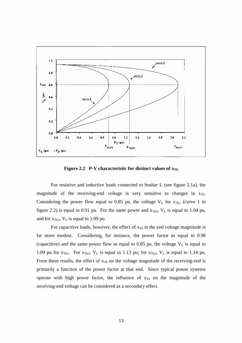
Using per unit based on the rated rms voltage at busbar L, three values for xTh

are considered: xTh1=0.7 pu, xTh2=0.5 pu and xTh3=0.3 pu. A sending-end voltage

VTh=1.12 pu is chosen to result in VL equal to 1.0 pu for PT equal to 1.0 pu and xTh2

equal to 0.5 pu. In figure 2.2, each curve represents the power transfer characteristic

for each one of the three values of xTh replaced into equation 2.3. Curve 1 is the P-V

characteristic for xTh1, curve 2 for xTh2, and curve 3 for xTh3.

In figure 2.2, the maximum available power for curve 1 is PMAP1= 0.93; for

curve 2 is PMAP2= 1.25 pu and for curve 3 is PMAP3= 2.08 pu. The three MAPs occur

at the same voltage VSM=0.79 pu. If the power PT varies without changing the power

factor (in this example, unity power factor), the MAP is always reached at the same

VSM. Changes in xTh do not modify the voltage at maximum power transfer, although

the MAP itself is modified. Analysing the P-V characteristics in figure 2.2, for a given

power demand and at a specified power factor (unity, in this example), the larger the

impedance of transference xTh, the larger the reduction of voltage magnitude at the

receiving end.

13

Figure 2.2 P-V characteristic for distinct values of xTh

For resistive and inductive loads connected to busbar L (see figure 2.1a), the

magnitude of the receiving-end voltage is very sensitive to changes in xTh.

Considering the power flow equal to 0.85 pu, the voltage VL for xTh1 (curve 1 in

figure 2.2) is equal to 0.91 pu. For the same power and xTh2, VL is equal to 1.04 pu,

and for xTh3, VL is equal to 1.09 pu.

For capacitive loads, however, the effect of xTh in the end voltage magnitude is

far more modest. Considering, for instance, the power factor as equal to 0.98

(capacitive) and the same power flow as equal to 0.85 pu, the voltage VL is equal to

1.09 pu for xTh1. For xTh2, VL is equal to 1.13 pu; for xTh3, VL is equal to 1.14 pu.

From these results, the effect of xTh on the voltage magnitude of the receiving-end is

primarily a function of the power factor at that end. Since typical power systems

operate with high power factor, the influence of xTh on the magnitude of the

receiving-end voltage can be considered as a secondary effect.

14

Changes in xTh affect mainly the transmission angle. If the active power PT

changes, the voltage VXTh produced by the line current &I crossing xTh also changes.

PT is related to the component of current &I in phase with &VL (active component).

Since xTh, in the present discussion, is assumed to be purely inductive, VXTh is

orthogonal to the in-phase current component (see figure 2.1b). Therefore, for typical

power systems, VXTh is quasi-orthogonal to &VL . Change in xTh modifies VxTh and,

consequently, the transmission angle δ between &VTh and &VL is altered. The reduction

of xTh, for example, results in the reduction of the voltage across it, for a given power

flow. As the transmission angle is directly related to the voltage across xTh (voltage

VXTh, in figure 2.1b), the transmission angle is also reduced.

To illustrate the effect of xTh into the transmission angle δ, the following

example is discussed: from equation 2.4 (unity power factor), for a power flow equal

to 0.85 pu, VTh equal to 1.12 pu and xTh1, the transmission angle δ is equal to 35.78°.

Considering the same PT=0.85 pu and VTh=1.12 pu but with xTh2, δ is equal to 21.33°;

for xTh3, δ is equal to 12.01°. The figures indicate a strong influence of the impedance

of transference xTh into the transmission angle δ.

Using equation 2.1 for the previous example, when the transfer power factor is

equal to 0.98 capacitive, the transmission angle δ for xTh1 is 29.03°. For xTh2, δ is

19.54°, and for xTh3, δ is 12.03°. Comparing the transmission angles for each one of

the three impedance of transference xTh for both unity and capacitive transfer power

factors, the influence of the transfer power factor on the transmission angle is small.

Regardless the transfer power factor (for typical values), the impedance of

transference xTh remains as the main variable that affects the transmission angle δ.

The stability of the power system is related to the transmission angle δ. When

the power is transferred at small transmission angle, the operating point of the ac is

distant from the steady-state limit, increasing the stability margin [49][51]. Both the

steady-state limit for power transfer and stability margin are defined in Section

2.4.1.2.

15

If the power demand at busbar L increases, a compensation of xTh might be

required to reduce the transmission angle and move the operating point away from the

steady-state stability limit, increasing the stability margin.

The transfer power factor also affects the P-V characteristic. The relation

between transferred power factor and power transfer characteristic is discussed in

Section 2.2.2.

2.2.2 The power transfer characteristic and the transfer

power factor (pfT)

Equations 2.1 and 2.2 relate the transferred power PT and the voltage VL to the

transfer power factor (cosφ). If PT and VL are individually affected by cosφ, so is the

relation between them, which is represented by the power transfer characteristic. If

the transfer power factor is capacitive, indicating an injection of reactive power into

the receiving end, reactive losses in xTh are partially (or totally, depending on the

amount of injected reactive power) compensated.

The effect of cosφ on the curve P-V is discussed in example 2.2. The same

simplified system shown in figure 2.1a is adopted for the analysis.

Example 2.2

Considering the same figure 2.1a as in the example 2.1, the voltage VTh is equal to

1.12 pu and xTh is equal to 0.5 pu. To define the power transfer characteristic, as in

Section 2.2.1, the load in Subsystem II varies from infinite to zero whilst VTh and xTh

remain constant. However, three loads with distinct power factors are considered.

16

The P-V characteristics, presented in figure 2.3, for three distinct transfer

power factors. In curve 1, the transfer power factor is pfT1=0.98 inductive (lagging);

in curve 2 is pfT2=1.0 (unity transfer power factor) and in curve 3 is pfT3=0.98

capacitive (leading). The transfer power factors pfT1, pfT2 and pfT3 are kept constant

during the variation of load for each one of the three P-V characteristics plotted in

figure 2.3. The transfer power factor clearly affects the power transfer characteristic.

Figure 2.3 Power transfer characteristic for distinct transfer power factor

From figure 2.3, when the power PT1 equals 1.0 pu, the voltage VL is equal to

0.81 pu for pfT1, in curve 1. For pfT2 (curve 2, unity transfer power factor) and the

same PT1, the voltage is equal to 1.0 pu. For pfT3 (curve 3), the voltage is equal to

1.12 pu. Therefore, the more capacitive the transfer power factor the higher the

voltage VL, for a given power PT.

17

Considering a second transferred power PT2 equal to 1.19 pu, it is not possible

to transfer such power with pfT1, since the maximum available power in curve 1 is

smaller than 1.19 pu. For pfT2, the voltage VL is equal to 0.9 pu, which is 10 %

smaller than the end voltage for power equal to 1.0 pu (PT1). For pfT3, VL is equal to

1.09 pu. Moreover, for the leading power factor pfT3 (curve 3), it is possible to

transfer up to 1.48 pu of power with a receiving-end voltage equal or higher than 0.9

pu.

The two cases discussed above are summarised in table 2.1.

Table 2.1 Effect of the transfer power factor on receiving-end voltage for two distinct values of power

cases (n) PTn VL1

(pfT1) VL2

(pfT2) VL3

(pfT3) 1 1.0 0.81 1.00 1.09

2 1.19 --- 0.9 1.12

Growth of transferred power does not necessarily results in an intense

reduction of the receiving-end voltage. For a leading power factor, for instance, the

voltage can be sharply reduced only in the vicinity of the MAP.

Referring to figure 2.3, if the transfer power factor is corrected, the maximum

available power can be significantly improved. In addition, by changing transfer

power factor, the maximum power can be transferred at an acceptable voltage drop at

the receiving end. Although the maximum power transfer is hardly considered under

steady-state operations, it might be a temporary solution following a major

disturbance in the ac system (transient condition).

From figure 2.3, the maximum available power PMAP1 is equal to 1.03 for pfT1

(curve 1), with the busbar voltage VLM1= 0.72 pu. PMAP2 is equal to 1.25 for pfT2

(curve 2), with VLM2= 0.79 pu. PMAP3 is equal to 1.53 for pfT3 (curve 3), with VLM3=

0.88 pu. These values are arranged in table 2.2.

18

Table 2.2 Maximum available power and respective receiving-end voltages

pfT VLM PMAP

0.98 0.72 1.03

1.00 0.79 1.25

-0.98 0.88 1.53

Correction of the transfer power factor can be achieved either by changing the

power factor of the load or by injecting reactive power (reactive shunt compensation)

into the busbar. Reactive shunt compensation is the usual solution to correct the

transfer power factor.

The transfer power factor is an important aspect to be considered in the power

transfer characteristic of the ac system. Power factor correction can affect both the

transmission angle and the voltage magnitude. However, it is normally associated to

shunt compensation, which is mainly used to control voltage magnitude. Aspects of

shunt compensation are discussed in Section 2.3.1.

The magnitude of the sending-end voltage, the third parameter that modifies

the power transfer characteristic, is discussed in Section 2.2.3.

2.2.3 The power transfer characteristic and the sending-

end voltage magnitude

According to equations 2.1 and 2.2, the power transfer characteristic is affected by the

magnitude of the sending-end voltage (VTh).

19

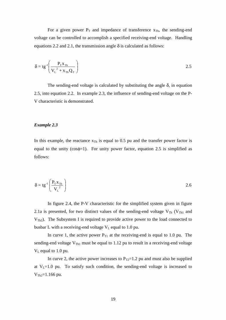
For a given power PT and impedance of transference xTh, the sending-end

voltage can be controlled to accomplish a specified receiving-end voltage. Handling

equations 2.2 and 2.1, the transmission angle δ is calculated as follows:

⎟⎟⎠

⎞⎜⎜⎝

⎛δ

TTh2

L

ThT1-

Qx+V

xPtg= 2.5

The sending-end voltage is calculated by substituting the angle δ, in equation

2.5, into equation 2.2. In example 2.3, the influence of sending-end voltage on the P-

V characteristic is demonstrated.

Example 2.3

In this example, the reactance xTh is equal to 0.5 pu and the transfer power factor is

equal to the unity (cosφ=1). For unity power factor, equation 2.5 is simplified as

follows:

⎟⎟⎠

⎞⎜⎜⎝

⎛δ

2L

ThT1-

V

xP tg= 2.6

In figure 2.4, the P-V characteristic for the simplified system given in figure

2.1a is presented, for two distinct values of the sending-end voltage VTh (VTh1 and

VTh2). The Subsystem I is required to provide active power to the load connected to

busbar L with a receiving-end voltage VL equal to 1.0 pu.

In curve 1, the active power PT1 at the receiving-end is equal to 1.0 pu. The

sending-end voltage VTh1 must be equal to 1.12 pu to result in a receiving-end voltage

VL equal to 1.0 pu.

In curve 2, the active power increases to PT2=1.2 pu and must also be supplied

at VL=1.0 pu. To satisfy such condition, the sending-end voltage is increased to

VTh2=1.166 pu.

20

Figure 2.4 Power characteristic for two distinct sending-end voltages

Based on the curves illustrated in figure 2.4, the influence of the magnitude of

the sending-end voltage on the power transfer characteristic is promptly demonstrated,

which implies that the control of the receiving-end voltage VL can be achieved by

controlling the sending-end voltage VTh.

The curves in figure 2.4 also suggest that the magnitude of the sending-end

voltage does not affect substantially the maximum available power, when compared

to the figures presented in Sections 2.2.1 and 2.2.2, at least for typical values of

sending-end voltages.

The results discussed in this section allows to infer that the control of one or

more variables involved in a power transfer, namely sending-end voltage, impedance

of transference and transfer power factor, modifies the power transfer characteristic

and, as a consequence, the operating condition of a power transmission system. Using

reactive compensation, the former two variables can be controlled. This is discussed

in Sections from 2.3 to 2.3.2.

21

2.3 Power Transfer and Reactive Compensation

According to previous discussions presented in Sections 2.2.1 and 2.2.2, changes in

impedance of transference and correction of transfer power factor effectively affect

the power transfer characteristic of a transmission system. If those parameters are

properly controlled, the power transfer characteristic can be modified to attend to a

required operating condition.

The control of the power transfer characteristic has traditionally been

performed by reactive compensation [49]. The reactive compensator can be either

shunt or series-connected (or even a combination of both connections) to the power

systems. There are many designs of reactive compensators, from the simple capacitor

bank mechanically switched to the modern thyristor-based controllers, such as the

static var compensator (SVC), the advanced SVC (ASVC) or the thyristor-controlled

series compensator (TCSC) [22][52][53][54][55][56]. Details on each one of the

possible designs for the reactive compensators are beyond the scope of this research.

However, the influence of shunt and series reactive compensations on the power

transfer characteristic is discussed in Sections 2.3.1 and 2.3.2.

2.3.1 Power transfer and shunt compensation

In the past, reactive shunt compensation used to be performed by merely switching on

and off capacitor and reactor banks into the ac system or by connecting over-excited

synchronous machine to the system as synchronous condenser. The advance of power

electronics in the last decades has contributed to the design of compact, highly

controllable shunt compensators.

22

Reactive shunt compensators supply part of reactive power required by the ac

system and they are normally used to maintain the local voltage at a specified

(ordained) value (or range of values). Figure 2.5 shows a shunt compensator

connected to the ac system presented in figure 2.1a.

Qsh

SVC

D

SUBSYSTEM I

XTh SUBSYSTEMII

LQ

LV

ThTP

PTT

ThV

Q

Figure 2.5 Shunt compensator connected to a simplified ac system

The shunt compensator illustrated in figure 2.5 could be a SVC [49] or any

compensator that provides both capacitive and inductive compensations. The SVC

injects reactive power Qsh into busbar L. The total reactive power reaching the busbar

L, QT, is now the sum of the reactive power required by the Subsystem II, QD, plus the

reactive power injected by the reactive compensator, Qsh. The injected reactive power

Qsh can be either leading (capacitive) or lagging (inductive), depending on the

requirements of the ac system. Considering an ideal operation of the SVC, for

instance, the voltage VL would be kept at a controlled value VLord.

In equation 2.2, when the voltage VLord is equal to VTh, the transmission angle

δ is related to the load angle φ as follows:

cos(δ+φ)=cos(φ) 2.7

23

To satisfy equation 2.7, the relation between the angles δ and φ must be:

φ = − δ2

2.8

Therefore, for changes in power flow, which would result in changes in

transmission angle δ, the load angle φ must be continuously modified to satisfy

equation 2.8. Substituting equation 2.8 into equation 2.1:

Th

2Th

T x

)(sinV =P

δ 2.9

At first glance, equation 2.9 does not seem directly related to the transfer

power factor (cosφ). However, after analysing equations 2.2 and 2.7, it is verified that

VL is kept to an ordained value for changes in power flow only if the load angle φ is

continually modified. In other words, it is necessary to control the transfer power

factor to keep VL at an ordained value. The shunt compensator performs such control.

A comparison between equations 2.3 and 2.9 can be established. Equation 2.3

relates PT to δ for resistive load connected to a busbar without voltage support whilst

equation 2.9 relates PT to δ in a busbar with voltage support, regardless of the load.

The maximum power transfer calculated using equation 2.9 is exactly twice the

maximum power transfer calculated using equation 2.3. Furthermore, the maximum

power calculated in equation 2.9 occurs at a given transmission angle δ which is twice

the angle δ calculated in equation 2.3 for the maximum power.

Examining equation 2.1 (a general condition) and equation 2.9, one can

deduce that a given active power is transferred at smaller transmission angle δ when

the receiving-end voltage is supported by reactive compensation. Additionally, the

maximum available power is greatly improved.

The conditions described on equations 2.1 and 2.2 have no practical meaning

when dealing with real transmission systems because only a narrow margin of

variation of voltage magnitude at the system busbars is allowed (usually 5% below or

above the nominal voltage). However, the comparison between equations 2.1 and 2.9

is justified since it illustrates the importance of supporting voltage for power transfer.

24

For long transmission lines, the midpoint shunt compensation is an alternative

to improve power transfer. Midpoint shunt compensation is presented in Section

2.3.1.1.

2.3.1.1 Midpoint shunt compensation

A feasible procedure to improve power transfer through long transmission lines whose

end voltages are already controlled is to place the shunt compensation into the middle

of the line, as illustrated in figure 2.6a [49].

To exemplify the mid-point shunt compensation, a long transmission line

connecting two identical subsystems is shown in figure 2.6a. The end voltages are

kept constant and represented by ideal voltage sources (Es and Er). A shunt reactive

compensator is placed into the middle of the transmission line (point m), splitting the

line series reactance into two halves (equal to xl/2). Each half of the transmission line

is represented by a π-equivalent circuit. The voltage at the midpoint is called Vm and

the shunt compensator injects the reactive current Ish into the point m.

The current Ish can be either capacitive or inductive, depending on the degree

of compensation required at the midpoint. The relation between the transmission line

shunt capacitance and the shunt compensator reactance can be expressed as follows:

k m =B

1

2Bc

γ 2.10

where: Bγ : compensating susceptance

Bc : total transmission line susceptance

25

Figure 2.6 Midpoint shunt compensation for a long transmission line

Considering the end voltages constant, the circuit presented in figure 2.6a can

be simplified, resulting in the circuit shown in figure 2.6b. The central susceptance,

in figure 2.6b is a combination of the compensator susceptance ( Bγ ) plus the

transmission line susceptance ( Bc ) and can be expressed as:

( )mk+= 12

BB c

central 2.11

If km is negative, the shunt compensator works as an inductance and its

susceptance lessens the transmission line susceptance.

26

On the other hand, if km is positive, the shunt compensator acts as a

capacitance, increasing Bc . If Bγ =− Bc /2 (inductive), km is equal to −1 and the

central susceptance is equal to zero.

Applying the Δ−Υ transformation to the circuit described in figure 2.6b, and

considering Es and Er constant (together they must absorb half of the reactive power

provided by the transmission line capacitance), the impedance of transference

between Es and Er can be expressed as:

)s1(x=x lTh − 2.12

where:

( )mcl k1

4

B

2

xs −= 2.13

Considering Es = Er = VTh and substituting equation 2.12 into 2.9, the power

equation can be described as:

)s1(x

)(sinV =P

l

2Th

T −δ

2.14

Applying the midpoint compensation to the system shown in figure 2.1a,

dividing xTh into two equal halves and keeping the busbar voltage VL equal to VTh,

equation 2.14 can be re-written as:

Th

2Th

T x

)2(sin2V =P

δ 2.15

Comparing now equation 2.9 with equation 2.15, the maximum power transfer

with shunt compensation in the middle of the transmission line impedance (equation

2.15) is twice the power transfer without midpoint compensation (equation 2.9).

27

The maximum power calculated using equation 2.15 occurs for a transmission

angle δ which is twice the δ for maximum power when no shunt compensation is

provided in the midpoint (equation 2.9). The compensation procedure by sectioning

the transmission line into two halves has been proposed to improve maximum

transmissible power in long transmission lines [46].

In figure 2.7, the power-angle (P−δ) characteristics calculated using equations

2.3, 2.9 and 2.15 are compared. Curve 1, which is computed using equation 2.3,

represents the P−δ characteristic of the simplified system presented in figure 2.1a,

without support in the voltage VL. Curve 2 represents the P−δ characteristic of the

system shown in figure 2.5, with VL constant and equal to VTh, and it is calculated

using equation 2.9. Curve 3 illustrates the P−δ characteristic for supported voltage at

the midpoint of the impedance xTh, according to figure 2.6a and it is calculated using

equation 2.15.

Figure 2.7 The effect of shunt compensation on power-angle characteristic

28

Despite considering the end voltages as ideally controlled and transmission

systems without losses, the results presented in the present section illustrate how shunt

compensation modifies the power transfer characteristic. It is possible to improve the

power transfer at small transmission angle by using shunt compensation. This

achievement has significant impact on the power system stability performance.

In Section 2.3.2, the influence of series compensation on power transfer

characteristic is presented.

2.3.2 Power transfer and series compensation

Capacitor (or capacitor bank) inserted in series with the transmission line has

traditionally performed series compensation. However, problems such as sub-

synchronous resonance [50] (which originates from the combination between

compensating capacitors and generator inductances), have justified the search for new

concepts in series compensation. The Thyristor-Controlled Series Compensator

(TCSC), which uses Thyristor-Switched Capacitor (TSC) in parallel with Thyristor-

Controlled Reactor (TCR), is one of the new controllers used as series compensators

which are sub-synchronous resonance free [25][26][42][57]. Furthermore,

controllable series compensation has been claimed to improve the power oscillation

damping and to re-direct the power flow, avoiding undesirable power loops [58].

To exemplify the effect of series compensation on the power transfer

characteristic, a generic reactive compensator xse is inserted in series with xTh in the

simplified system represented in figure 2.1a. The modified system is illustrated in

figure 2.8.

29

Th

SUBSYSTEM I

VTh

XThSUBSYSTEM

II

sex QTTP

VL

L

Figure 2.8 Series compensation in a simplified system

As the reactance xse is inherently capacitive, it is subtracted from xTh, which is

essentially inductive. Equation 2.1 is then modified, resulting in equation 2.16 as

follows:

)cos()k1(x

)cos()(sinV =P

seTh

2Th

T φ−φ+δδ

2.16

where Th

sese

x

xk = : compensating index

The compensating index kse modifies the impedance between busbar Th and

busbar L, in figure 2.8. For a constant VL, equation 2.16 becomes:

)k1(x

)(sinVV =P

seTh

LThT −

δ 2.17

The series compensation reduces the impedance of transference between two

busbars. Therefore, for a given power transfer, the voltage across the impedance of

transference also decreases, resulting in a smaller transmission angle between &VTh

and &VL .

30

On the other hand, when using reactive series compensation, the power

transfer can be increased at a reduced transmission angle, keeping the operating point

distant from the maximum power transfer. Power transfer at a small transmission

angle is especially important when the transmission line is an inter-tie, connecting two

major subsystems. Large transmission angles can result in loss of synchronism

between interconnected machines when the ac system is subject to disturbances.

Several papers have reported improvement on power system stability when series

reactive compensation is used [22][28][31][59].

Curve 1, in figure 2.9, which is drawn from values calculated using equation

2.17, represents the effect of series compensation on the power-angle characteristic.

Curve 2 represents the power-angle characteristic without series compensation

( )kse = 0 . In both cases, VL is considered constant and equal to VTh.

Figure 2.9 The effect of series compensation on power-angle characteristic

31

Based on figure 2.9, series compensation increases the maximum power, from

Pmax to Pmax' . However, the transmission angle for maximum power is unchanged.

This is readily verified by examining equations 2.16 and 2.17, since series

compensation affects only the reactance, without interfering in the transmission angle.

The analysis conducted in Sections 2.2 and 2.3 consider generic impedance of

transference. However, the transmission line is the electrical component responsible

for transferring power in electrical power systems. The behaviour of the transmission

line as a power transfer-limiting factor, regarding both its electric parameters and

class of voltage, is discussed in Section 2.4.

2.4 Transmission Line and Power Transfer

In electrical power systems, the transmission lines are the component responsible for

transferring power from a source to a load or, broadly speaking, from one point to

another in the system. Paradoxically, the transmission line also limits power transfer,

due to its own capability characteristics. St. Clair first introduced practical concepts

on the capability of transmission lines in the fifties [60]. The main factors limiting the

transmission line capability are the system voltage level, the thermal rating (line

current) steady-state stability limit and the exchange of reactive power among

transmission line reactances. Resistive losses and temperature are also limiting

factors, but of limited significance. Voltage level and thermal rating are based on

constructive aspects of the transmission line, whilst steady-state stability limit and

reactive exchange depend on the dynamic comportment of the power system.

The system voltage level is usually defined in the planning stage, according to

the particularities of the system regarding power generation and distribution, such as

available power sources, expected power demand, electrical distance between

generation and load, among others.

32

Thermal rating is usually a limiting factor on the capability of relatively short

transmission line, whose length is shorter than 80 km [50 miles] at fundamental

frequency of 60 Hz [60]. Thermal rating is only defined considering constructive

aspects of a transmission line. Then, it becomes more an economical rather than an

operational problem. This is especially true for a voltage level of 138 kV or below.

At levels such as extra high voltage (EHV, from 230 kV up to 765 kV) and

ultra high voltage (UHV, above 756 kV), the corona discharges and the field effects

will require transmission line designs which result in a high thermal capability for a

transmission line [61].

As the length of transmission line increases, the other two main factors,

namely steady-state stability limit and reactive exchange, become the major limiting

factors in the transmission line capability. The capability limits of the transmission

line, regarding reactive exchange and steady-state stability, are discussed in Section

2.4.1.

2.4.1 Capability limits for transmission lines

The capability of the transmission line is usually expressed in terms of surge

impedance loading (SIL). The surge impedance loading of a transmission line is

defined as the power that flows in a lossless transmission line ending in a resistive

load equal to the transmission line surge impedance. The surge impedance (ZC) for a

lossless transmission line is given by:

ZC = l

c 2.18

where: l: transmission line inductance (per unit of length)

c: transmission line capacitance (per unit of length)

33

The surge impedance loading (SIL) is expressed as:

( )SIL =

V

Z

phase-phase

2

C

2.19

where: Vphase-phase: rms phase-to-phase voltage at the transmission line end, in kV

ZC: transmission line surge impedance, expressed in ohms or without unit

If ZC is expressed in ohms, SIL is given in MW. If ZC has no unit, SIL is

given in kV2.

If the transmission line ends at its surge impedance, the voltage at the sending

end is equal to the voltage at the receiving end. In this case, a line charging

(capacitance) effect offsets the reactive absorbed by the transmission line inductance,

resulting in a net reactive power in the transmission line equal to zero. In this

condition, the transmission line is called flat or infinite line.

Power transmission lines rarely end in surge impedance. If the resistive load

connected to the transmission line end is larger than the surge impedance ZC, there is

a surplus of reactive power provided by the transmission line capacitance. This is

often referred to as light loading condition. The voltage at the transmission line

receiving-end is higher than the voltage at the sending end. Conversely, for an ending

resistive load smaller than ZC, referred to as heavy loading condition, reactive losses

exceed the reactive power provided by the transmission line capacitance. In this case,

the receiving-end voltage is smaller than the sending-end voltage. The transmission

line may be subject to a variation between heavy and light loading due to dynamic

changes in the load. The result is a voltage fluctuation at the receiving-end of the

transmission line, associated to reactive exchange imposed by the transmission line.

34

2.4.1.1 Reactive Power and the Transmission Line

The reactive power absorbed by the transmission line inductance, Ql, is a function of

the current passing through the transmission line and it is expressed according to

equation 2.20. On the other hand, the reactive power provided by the transmission

line capacitance, Qc, is a function of the rated voltage at the transmission line end and

it is expressed by equation 2.21.

Q I x2l l= 2.20

QV

x

2

cc

= 2.21

where: I: rms current through the transmission line

V: rms phase-to-phase voltage

xl: transmission line inductance ( )lengthl freq., fund.f,lfl2x l ==π=

xc: transmission line capacitance ⎟⎠⎞

⎜⎝⎛ ==

π= lengthlfreq., fund.f,l

fc2

1x c

Qc can also be expressed as a function of the line-charging current (Ichg),

according to equation 2.22. Line-charging current, defined in equation 2.23, is the

current resultant from the charging and discharging of a transmission line due to

alternating voltage [62]. Ichg flows even if the receiving end of the transmission line is

an open-circuit. As the voltage varies along the transmission line, the rated voltage is

normally used to calculate the line-charging reactive power.

Q I Vchgc = 3 2.22

IV

xchg =

c 3 2.23

35

2.4.1.2 Steady-state stability and power-angle (P-δ)

characteristic

The steady-state stability is defined as the ability of the power system to sustain the

transfer of power from one terminal to another for small changes in load [50][51][63].

The limit of steady-state stability was defined as “a condition of a linear system or one

of its parameters which places the system on the verge of instability [51].”

The steady-state stability is associated with the voltage across the transmission

line reactance. As the current crossing the transmission line increases, the voltage

across the transmission line reactance also increases. The voltage across this

reactance is related to the angle between the voltage vectors at the ends of

transmission line. This angle was previously defined as transmission angle. The

larger the voltage across the transmission line, the larger the transmission angle.

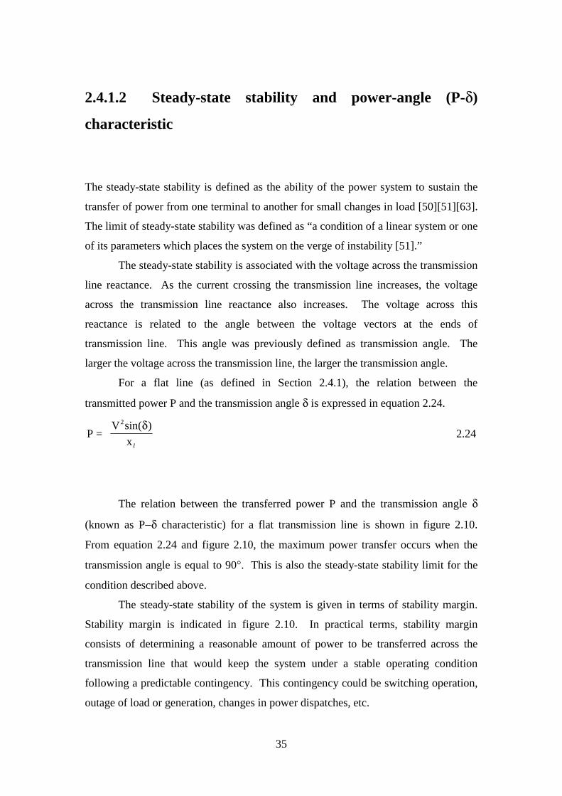
For a flat line (as defined in Section 2.4.1), the relation between the

transmitted power P and the transmission angle δ is expressed in equation 2.24.

P = V sin )

x

2 (δ

l

2.24

The relation between the transferred power P and the transmission angle δ

(known as P−δ characteristic) for a flat transmission line is shown in figure 2.10.

From equation 2.24 and figure 2.10, the maximum power transfer occurs when the

transmission angle is equal to 90°. This is also the steady-state stability limit for the

condition described above.

The steady-state stability of the system is given in terms of stability margin.

Stability margin is indicated in figure 2.10. In practical terms, stability margin

consists of determining a reasonable amount of power to be transferred across the

transmission line that would keep the system under a stable operating condition

following a predictable contingency. This contingency could be switching operation,

outage of load or generation, changes in power dispatches, etc.

36

Figure 2.10 Power angle (P-δ) characteristic

Stability margin is defined according to equation 2.25:

Stability Margin (%) =P P

Pmax rated

max

−= −1 sinδ 2.25

The steady-state stability margin, derived from the P-δ characteristic, is based

on fixed voltage magnitude at the transmission line ends. This presumes that the

reactive power absorbed by the transmission line is supplied by the ac system.

Therefore, the steady-state stability is fundamentally influenced by the voltage across

the transmission line series reactance, rather than by the net reactive power exchanged

between the transmission line and the ac system.

37

2.4.2 St. Clair capability curves

In the early fifties, H. P. St. Clair related the length with the capability of the

transmission line by the curves known as St. Clair’s capability curves [60]. St. Clair’s

capability curves, which were empirically derived for transmission lines up to 1000

km (600 miles), are shown in figure 2.11a. These curves were later analytically

demonstrated [61]. The analytical curve, which is very similar to that shown in figure

2.11a, is shown in figure 2.11b.

The analytical demonstration [61] of the empirical St. Clair’s capability curves

clarifies the influence of each limiting factor on the transmission line capability. The

analytical curve was created using two of the capability limiting factors previously

discussed: voltage drop at the transmission line receiving end and steady-state

stability margin.

In [61], the authors assume a maximum voltage drop at the receiving end equal

to 5% and a stability margin equal to 35%. In figure 2.11b, curve 1 indicates the

capability curve for a stability margin of 35%, considering a flat transmission line.

Curve 2 shows the capability curve for a maximum voltage drop of 5%. Taking the

more conservative value of both curves, the composed capability curve (in pu of SIL)

matches the empirical curve presented in [60]. The region of voltage drop dominates

the capability limits for transmission lines from 80 km (50 miles) to 320 km (200

miles). On the other hand, the region of stability margin limits the capability of

transmission lines longer than 320 km. The limiting regions are identified in figure

2.11b.

Voltage drop and steady-state stability limits, as opposed to system voltage

level and resistive losses, can be dynamically changed if the control of reactive power

and transmission angle, respectively, can be established. In the Section 2.2, the

relation between the system voltage vectors and the power transfer characteristic was

demonstrated.

38

(a) an empirical approach

(b) an analytical approach

Figure 2.11 Transmission line capability curves

39

2.5 Conclusion

The analysis conducted in this Chapter 2 presented the limits of power transfer in

typical electric power systems.

Power transfer (P-V) characteristics were plotted using simplified systems, for

distinct conditions of load and generation. The effect of three system variables

(namely the sending-end voltage magnitude, the impedance of transference between

the sending and the receiving ends, and the transfer power factor) on the P-V

characteristic was investigated. If the three system variables are efficiently controlled,

the active power can be transferred according to a pre-defined operating condition.

The series and the shunt reactive compensations were proved to have a strong

influence on the power transfer characteristic. Therefore, reactive power

compensators can be used to control the operating condition in a power transfer

operation.

Power transfer limits based on transmission line characteristics were

introduced using the St. Clair’s capability curves. Limiting capability factors such as

voltage drop and steady-state stability were described. Although capability criteria

have been associated to the transmission line parameters, the power transfer limitation

would involve the total reactance between two busbars, including transformers, series

and shunt system components, etc. Power controllers can be used to change the

equivalent reactance between two busbars and to improve the power transfer

capability.