CHAPTER 7: STATISTICAL TECHNIQUES FOR CLINICAL TRIALS

7.1 DEVELOPMENT PLAN

The efficacy and safety of principal products should be demonstrated by clinical trials. The broad

aim of the process clinical development is to find out whether there is a dose range and effective,

to the extent that the risk-benefit relationship is acceptable. Satisfying this broad aims usually

requires an ordered programme of clinical trials, each with its own specific objectives. This

should specified in clinical plan or a series of plans, with appropriate decision points and

flexibility to allow modification as knowledge accumulates. A marketing application should

clearly describe the main content of such plans, and contribution made by each trial.

CONFIRAMATORY TRIAL

A confirmatory trial is an adequately controlled trial in which the hypotheses are stated in

advance and evaluated. As a rule, confirmatory trials are necessary to provide firm evidence of

efficacy or safety. In such trials the key hypothesis of interest follows directly from the trial’s

primary objective, is always pre-defined, and is the hypothesis that is subsequently tested when

the trial is complete. In a confirmatory trial it is equally important to estimate with due precision

the size of the effects attribute to the treatment of interest and to relate these effects to their

clinical significance.

EXPLORATORY TRIALS

The rationale and design of confirmatory trials nearly always resets on earlier clinical work

carried out in a series of exploratory studies. Like all clinical trials, these exploratory studies

should have clear and precise objective. However, in contrast to confirmatory trials, their

objectives may not always lead to simple tests pre-defined hypotheses. In addition, exploratory

trials may sometimes require a more flexible approach to design so that changes can be made in

response to accumulating results. Their analysis may entail data exploration; test of hypothesis

may be carried out, but the choice of hypothesis may be data dependent.

SCOPE OF TRIALS

POPULATION

In the earlier phases of drug development the choice of subjects for a clinical trial may be

heavily influenced by the wish to maximize the chance of observing specific clinical effects of

interest, and hence they may come from a very narrow subgroup of the total patient population

for which the drug may eventually be indicated. However by the time the confirmatory trials are

undertaken, the subjects in the trials should more closely mirror the target population. No

individual clinical trial can be expected to be totally representative of future users, because of the

possible influences of geographical location, the time when it is conducted, the medical practices

of particular investigators and clinics, and so on. However the influence of such factors should

be reduced whenever possible, and subsequently discussed during the interpretation of the trial

results.

VARIABLES

The primary variable or target variable or primary end point should be the variable capable of

providing the most clinically relevant and convincing evidence directly related to the primary

objective of the trial. There should generally be only one primary variable. This will usually be

an efficacy variable, because the primary objective of most confirmatory trial is to provide strong

scientific evidence regarding efficacy.

It may sometimes be desirable to use more than one primary variable, each of which ( or a subset

of which) could be sufficient to cover the range of effects of the therapies. The planned manner

of interpretation of this type of evidence should be carefully spelled out. It should be clear

whether an impact on any of the variables, some minimum number of them, or all of them,

would be considered necessary to achieve the trial objectives. The primary hypothesis or

hypotheses and parameters of interest (e.g. mean, percentage, distribution) should be clearly

stated to the primary variables identified, and the approach to statistical inference described. The

effect on the type I error should be given in the protocol. The extent of intercorrection among the

proposed primary variable may be considered in evaluating the impact on type I error. If the

purpose of the trial is to demonstrate effects on all of the designated primary variables, then there

is no need for adjustment of the type I error, but the impact on type II error and sample size

should be carefully considered.

Secondary variables are either supportive measurements related to the primary objective or

measurement of effects related to the secondary objectives. Their pre-definition in the protocol is

also important, as well as an explanation of their relative importance and roles in interpretation

of trials results. The number of secondary variables should be limited and should be related to

the limited number of questions to be answered in the trial.

Composite variable cannot be selected from multiple measurements associated with the primary

objective, another useful strategy is to integrate or combine the multiple measurements into a

single or ‘composite’ variable, using a pre-defined algorithm. Indeed the primary variable

sometimes arises as a combination of multiple clinical measurements (e.g. rating scales used in

arthritis, psychiatric disorders and elsewhere). This approach addresses multiplicity problem

without requiring adjustment to type I error. The method of combining multiple measurements

should be specified in the protocol, and an interpretation of the resulting scale should be

provided in terms of the size of a clinically meaningful and validated. When rating scale is used

as a primary variable, it is especially important to address such factors as content validity, inter-

and intra-rater, reliability and responsiveness for detecting changes in the severity of diseases.

Global Assessment Variables are developed to measure the overall safety, overall efficacy, and

/or overall usefulness of a treatment. This type of variable integrates objective variables and the

investigator’s overall impression about the state or change in the state of the subject, and is

usually a scale of ordered categorical ratings. A problem with global usefulness variables is that

their use could in some cases lead to the result of two products being declared equivalent despite

having very different profiles of beneficial and adverse effects. Therefore it is not advisable to

use a global usefulness variable as a primary. If global usefulness is specified as primary, it is

important to consider specific efficacy and safety outcomes separately as additional primary

variables.

When the direct assessment of the clinical benefit to the subject through observing actual clinical

efficacy is not practical, indirect criteria may be considered. Commonly surrogate variables are

used in a number of indications where they are believed to be reliable predictors of clinical

benefit. There are two principles concerns with the introduction of any proposed surrogate

variable. First, it may not be a true predictor of the clinical outcome of interest. For example it

may measure treatment activity associated with one specific pharmacological mechanism, but

may not provide full information on the range of actions and ultimate effects of the treatment,

whether positive or negative.

Dichotomisation or other categorization of continuous or ordinal variable may sometimes be

desirable. Criteria of ‘success’ and ‘response’ are common examples of dichotomies which

require precise specification in terms of , for example, a minimum percentage improvement

(relative to baseline) in a continuous variable, or a ranking categorized as at or above some

threshold level (e.g. ‘good’) on an ordinal relevance. The criteria for categorization should be

pre-defined and specified in the protocol, as knowledge of trial results could easily bias the

choice of such criteria. Because categorization normally implies a loss of information, a

consequence will be a loss of power in the analysis ; this should be accounted for in the sample

size calculation.

7.2 TECHNIQUES TO AVOID BIAS

BLINDING

Blinding or masking is intended to limit the occurrence of conscious and unconscious bias in the

conduct and interpretation of a clinical trial arising from the influence which the knowledge of

treatment may have on the recruitment and allocation of subjects, their subsequent care, the

attitudes of subjects to the treatments, the assessment of end-points, the handling of withdrawals,

the exclusion of data from analysis, and so on. The essential aim is to prevent identification of

the treatments until all such opportunities for bias have passed.

In a single-blind trial the investigator and or his staff are aware of the treatment but the subject is

not or vice versa. In open-label trial is all knows the identity of the treatment. A double-blind

trial is one in which neither the subject nor any of the investigator or sponsor staff who are

involved in the treatment received. This level of blinding is maintained throughout the conduct

of trial, and only when the data are cleaned to an acceptable level of quality will appropriate

person be unblended. Breaking the blind should be considered only when the subject’s physician

for the subject’s care deems knowledge of the treatment assignment essential.

RANDOMIZATION

Randomization introduces a deliberate element of change into the assignment of treatment to

subjects in a clinical trial. During subsequent analysis of the trial data, it provides a sound

statistical basis for the quantitative evaluation of the evidence relating to treatment effects. It also

tends to produce treatment groups in which the distributions of prognostic factors, known and

unknown are similar. In combination with blinding, randomization helps to avoid possible bias in

the selection of subjects arising from the predictability of treatment assignments. Although

unrestricted randomization is an acceptable approach, some advantages can generally be gained

by randomizing subjects in blocks. This helps to increase the comparability of the treatment

groups, particularly when subject characteristics may change over time, as a result, for example

of changes in recruitment policy. In multicenter trials the randomization procedures should be

organized centrally. It is advisable to have a separate random scheme for each center. More

generally stratification by important prognostic factors measured at baseline may sometime be

valuable in order to promote balanced allocation within strata; this has greater potential benefit in

small trials. The use of more than two or three stratification factors is rarely necessary, is less

successful at achieving balance and is logistically troublesome. Dynamic allocation is an

alternative procedure in which the allocation of treatment to a subject is influenced by the current

balance of allocated treatments and, in a stratified trial, by the stratum to which the subject

belongs and the balance within that stratum. Deterministic dynamic allocation procedures should

be avoided and an appropriate element of randomization should be incorporated for each

treatment allocation.

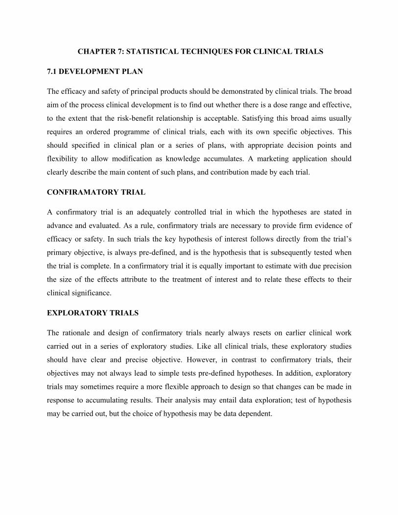
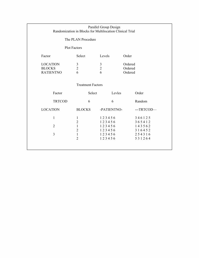
The following SAS Macro is used to generate randomization schedule for parallel design.

Proc plan ORDERED seed = 27370;

title 3, parallel Group Design

title 4 Randomization in Blocks for Multilocation Clinical Trial’:

factors LOCATION =3 BLOCKS =2 PATENTNO =6;

treatments TATCOD = 6 random;

output out=dbg 1 TATCOD nvals = (1 2 3 4 5 6 ) random ;

run ;

data dbg2 dbg3 dbg4;

set dbg1

if location =1 then output dbg2;

if location =2 then output dbg3;

if location =3 then output dbg4;

run;

data dbg5;

set dbg2 dbg3 dbg4;

run;

PROC SORT DATA = DBG5;

BY LOCATION BLOCKS PATIENTNO;

RUN;

Proc print data =dbg5;

run;

proc plan ordered seed = 27370;

title 3, parallel Group Design

title 4 ‘Randomisation in Blocks for Multilocation Clinical Trial’:

factors LOCATION =3 BLOCKS =2 PATENTNO =6;

treatments TATCOD = 6 random;

output out=dbg 1 TATCOD nvals = (‘A’ ‘A’ ‘A’ ‘B’ ‘B’ ‘B’ ) random

run;

PROC SORT DATA = DBG6;

BY LOCATION BLOCKS PATENTINO;

RUN;

Data dbg7;

Merge dbg5 dbg6;

By LOCATION BLOCKS PATIENTINO;

run;

Proc print data = dbg7;

run;

The SAS System Parallel Group Design

Randomization in Blocks for Multilocation Clinical Trial The PLAN Procedure Plot Factors Factor Select Levels Order LOCATION 3 3 Ordered BLOCKS 2 2 Ordered RATIENTNO 6 6 Ordered Treatment Factors Factor Select Levles Order TRTCOD 6 6 Random LOCATION BLOCKS -PATIENTNO- ---TRTCOD— 1 1 1 2 3 4 5 6 3 4 6 1 2 5 2 1 2 3 4 5 6 3 6 5 4 1 2 2 1 1 2 3 4 5 6 1 4 3 5 6 2 2 1 2 3 4 5 6 3 1 6 4 5 2 3 1 1 2 3 4 5 6 2 5 4 3 1 6 2 1 2 3 4 5 6 5 3 1 2 6 4

Parallel Group Design Randomization in Blocks for Multilocation Clinical Trial

Obs Location Blocks PATIENTNO TRTCOD

1 1 1 1 6 2 1 1 2 1 3 1 1 3 3 4 1 1 4 5 5 1 1 5 4 6 1 1 6 2 7 1 2 1 6 8 1 2 2 3 9 1 2 3 2

10 1 2 4 1 11 1 2 5 5 12 1 2 6 4 13 2 1 1 5 14 2 1 2 1 15 2 1 3 6 16 2 1 4 2 17 2 1 5 3 18 2 1 6 4 19 2 2 1 6 20 2 2 2 5 21 2 2 3 3 22 2 2 4 1 23 2 2 5 2 24 2 2 6 4 25 3 1 1 4 26 3 1 2 2 27 3 1 3 1 28 3 1 4 6 29 3 1 5 5 30 3 1 6 3 31 3 2 1 2 32 3 2 2 6 33 3 2 3 5 34 3 2 4 4 35 3 2 5 3 36 3 2 6 1

Parallel Group Design Randomization in Blocks for Multilocation Clinical Trial

The PLAN Procedure Plot Factors Factor Select Levels Order LOCATION 3 3 Ordered BLOCKS 2 2 Ordered RATIENTNO 6 6 Ordered Treatment Factors Factor Select Levles Order TRTCOD 6 6 Random LOCATION BLOCKS -PATIENTNO- ---TRTCOD— 1 1 1 2 3 4 5 6 3 4 6 1 2 5 2 1 2 3 4 5 6 3 6 5 4 1 2 2 1 1 2 3 4 5 6 1 4 3 5 6 2 2 1 2 3 4 5 6 3 1 6 4 5 2 3 1 1 2 3 4 5 6 2 5 4 3 1 6 2 1 2 3 4 5 6 5 3 1 2 6 4

Parallel Group Design Randomization in Blocks for Multilocation Clinical Trial

Obs Location Blocks PATIENTNO TRTCOD

1 1 1 6 B 2 1 1 1 A 3 1 1 3 A 4 1 1 5 B 5 1 1 4 B 6 1 1 2 A 7 1 2 6 B 8 1 2 3 A 9 1 2 2 A

10 1 2 1 A 11 1 2 5 B 12 1 2 4 B 13 2 1 5 B 14 2 1 1 A 15 2 1 6 B 16 2 1 2 A 17 2 1 3 A 18 2 1 4 B 19 2 2 6 B 20 2 2 5 B 21 2 2 3 A 22 2 2 1 A 23 2 2 2 A 24 2 2 4 B 25 3 1 4 B 26 3 1 2 A 27 3 1 1 A 28 3 1 6 B 29 3 1 5 B 30 3 1 3 A 31 3 2 2 A 32 3 2 6 B 33 3 2 5 B 34 3 2 4 B 35 3 2 3 A 36 3 2 1 A

7.3 INTERIM ANALYSIS

An interim analysis is any analysis to compare treatment arms with respect to efficacy or safety

at any time prior to formal completion of a trial. Under certain conditions, it is convenient and

sometimes prudent to look at data resulting from a study prior to its completion in order to make

a decision to abort the study early or to increase the sample size, for example. This is particularly

compelling for a clinical study involving a disease that is life threatening, is expensive, and /or is

expected to take a long time to complete. A study may be stopped, for example, if the test

treatment can be shown to be superior early on in the study. However, if the data are analyzed

prior to study completion, a penalty is imposed in the form of lower significance level to

compensate for the multiple looks at the data (i.e. to maintain the overall significance level at

alpha). The penalty takes the form of an adjustment of the alpha level to compensate for the

multiple looks at the data. For example, if the significance level is 0.05 for a single look, two

books will have an overall significance level of approximately 0.08.

In addition to the advantage (time and money) of stopping a study early when efficacy is clearly

demonstrated, there may be other reasons to shorten the duration of a study, such as stopping

because of drug failure, modifying the number of patients to be included, modifying dose, etc. if

interim analyses are made for these purposes in Phase III pivotal trials, an adjusted level is

needed.

A very important feature of interim analyses is the procedure of breaking the randomization

code. One should clearly specify who has access to the code and how the blinding of the study is

maintained. The execution of an interim analysis should be a completely confidential process

because unblended data and results are potentially involved. All staff involved in the conduct of

the trial should remain blind to the results of such analyses, because of the possibility that their

attitudes to the trial will be modified and cause changes in the characteristics of the patients to be

recruited or biases in treatment comparisons. This principle may applied to all investigator staff

and to staff employed by the sponsor except for those who are directly involved in the execution

of the interim analysis. Investigators should only the informed about the decision to continue or

to discontinue the trial or to implement modifications to trial procedures.

An interim trial analysis may also be planned to adjust sample size. In this case, a full analysis

should not be done. The analysis should be performed when the study is not more than half done,

and only the variability should be estimated (not the treatment differences). Under the

conditions, no penalty need be assessed. However if the analysis is one near the end of the trial

or if the treatment differences are computed, a penalty is required.

Following table shows the probability levels needed for significance for k looks (k analyses) at

the data according to O’Brien and Flemming, where the data are analyzed at equal intervals

during patient enrollment. For example, if the data are to be analyses or stages, including the

final analysis), the analysis should be done after 1/3rd , 2/3rd and all of the patients have been

completed.

Significance Levels for two-Sided Group Sequential studies with an Overall Significance-Level

of 0.05. (according to O’Brien and Flemming)

Number of analyses

(stages)

Analysis Significance

Level

2 First 0.005

Final 0.048

3 First 0.0005

Second 0.014

Final 0.045

4 First 0.0005

Second 0.004

Third 0.019

Final 0.043

Final 0.045

5 First 0.00001

Second 0.001

Third 0.048

Fourth 0.023

Final 0.041

For example, a study with 300 patients (150) patients in each of two groups) is considered for

two interim analyses. The first analysis is performed after 100 patietns are completed (50 per

group) at the 0.0005 level. To show statistically significant, the product differences must be very

large or obvious at this low level. If not significant analyze the data after 200 patients are

completed. A significant level of 0.014 must be reached to terminate the study. The final analysis

must meet the 0.045 levels for the products to be considered significantly different.

7.4 SAMPLE SIZE DETERMINATION

The number of subjects in a clinical trial should be large enough to provide a reliable answer to

the questions addressed. This number is usually determined by the primary objective of the trial.

If the sample size is determined on some other basis, then this should be made clear and justified.

For example, a trial sized on the basis of safety questions or requirements or important secondary

objectives may need larger numbers of subjects than a trial sized on the basis of the primary

efficacy question.

Using the usual method for determining the appropriate sample size, the following items should

be specified; a primary variable, the test statistics, the null hypothesis, the alternative hypothesis,

the probability of erroneously rejecting null hypothesis (the Type I error), and the probability of

erroneously failing to reject null hypothesis (the Type II error) as well as the approach to dealing

with the withdrawal and protocol deviations.

In confirmatory trials, assumptions should normally be based on published data or on the results

of earlier trials. The treatment difference to be based on a judgment concerning the minimal

effect, which has clinical relevance in the management of patients, or on a judgment concerning

the anticipated effect of new treatment, where this is larger. Conventionally the probability of

type I error is set to 5% or less or as dictated by any adjustments made necessary for multiplicity

considerations; the precise choice may be influenced by the prior plausibility of the hypothesis

under test and the desired impact of the results. The probability of the type I error is

conventionally set at 10% to 20% ; it is in the sponsor’s interest to keep this figure as low as

feasible especially in the case of trial that difficult or impossible to repeat.

The sample size of an equivalence or a non-inferiority trial should normally be based on the

objective of obtaining a confidence interval for the treatment different that shows that the

treatment differ at most by a clinically acceptable difference. When the power of an equivalence

trial is assessed at zero difference, then the sample size needed to achieve this power is

underestimated if the true difference is not zero. When the power of a non-inferiority trial is

assessed at a true difference of zero, then the sample size necessary to achieve this power is

underestimated if the effect of the investigational product is less than of active control. The

choice of a ‘clinically acceptable’ difference needs justification with respect to its meaning for

future patients, and may be smaller than the ‘clinically relevant’ difference referred to above in

the context of superiority trials to designed to establish that a difference exists. The exact sample

size in a group sequential trial cannot be fixed in advance because it depends upon the play of

chance in combination with the chosen stopping guideline and true treatment difference. The

design of the stopping guideline should take into account the consequent distribution of the

sample size, usually embodied in the expected and maximum sample sizes.

Suppose that a clinical trial researcher want to compare the effect of two drugs, A and B, on

systolic blood pressure (SBP). He has enough resources to recruit 25 patients for each drug. Hoe

big is the underlying effect size to detect? That is what is the population difference in mean SBP

between patients using drug A and patients using drug B? Of course, this is unknown. But one

can make an educated guess. Then the power analysis determines the chance of detecting this

conjectured effect size. For example if you have some results from a previous study involving

drug A, and you believe that the mean SBP for drug B differs by about 10% from the mean SBP

for drug A. If the mean SBP for drug A is 120, you thus posit an effect size of 12. What is the

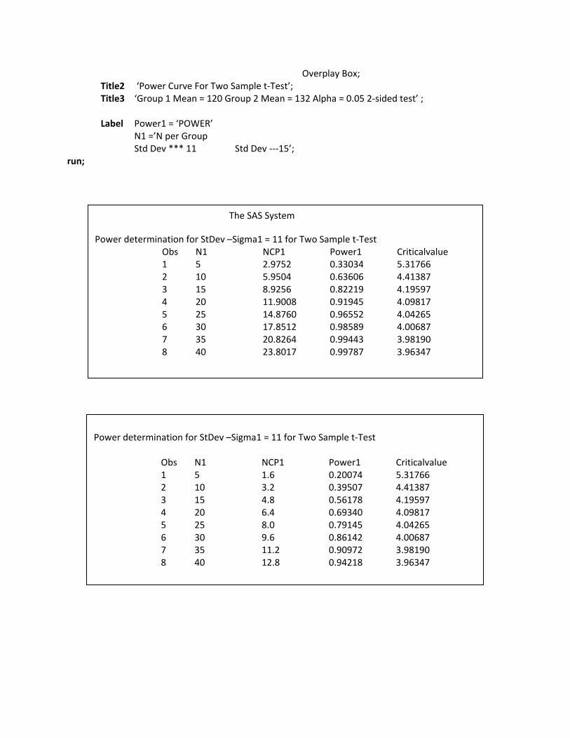
inherent variability in SBP? Suppose previous studies involving drug A have shown the standard

deviation of SBP to be between 11 and 15, and that the standard deviations are expected to be

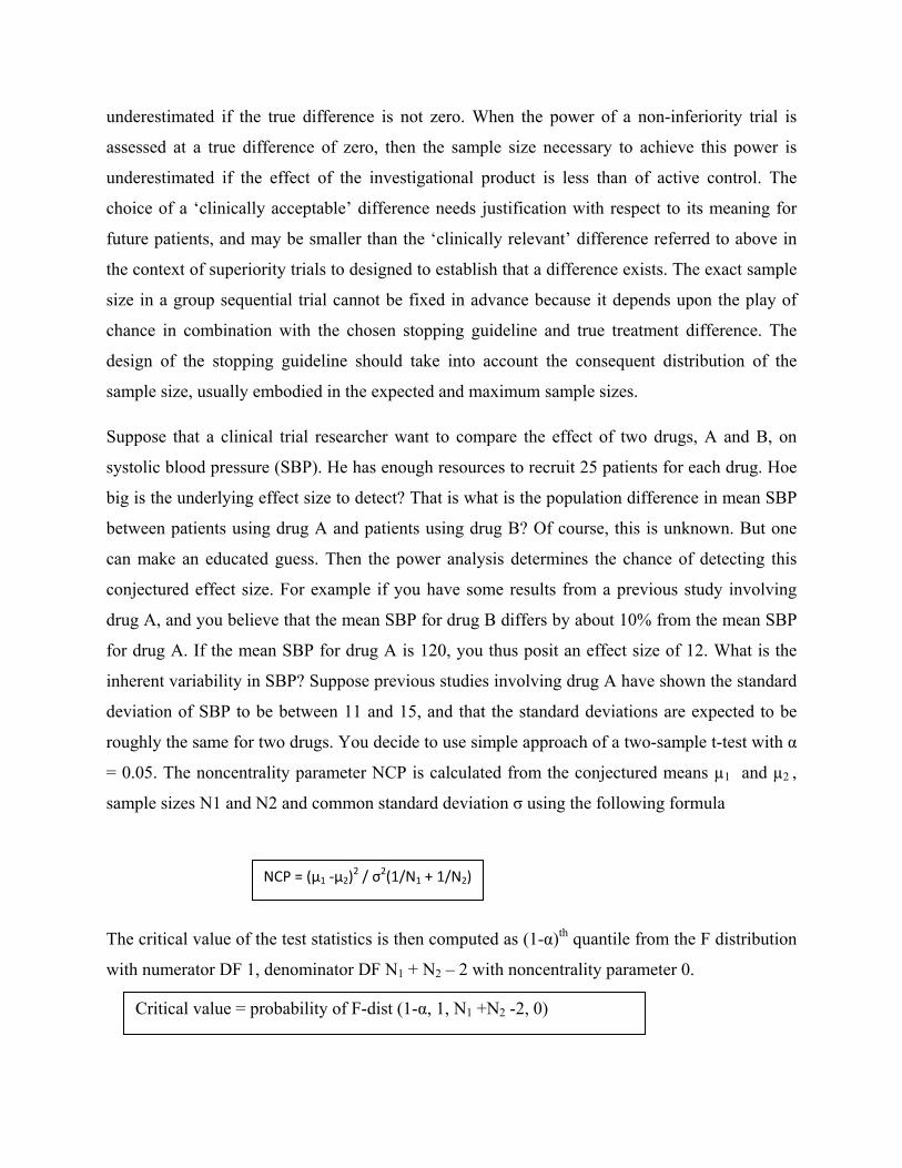
roughly the same for two drugs. You decide to use simple approach of a two-sample t-test with α

= 0.05. The noncentrality parameter NCP is calculated from the conjectured means µ1 and µ2 ,

sample sizes N1 and N2 and common standard deviation σ using the following formula

The critical value of the test statistics is then computed as (1-α)th quantile from the F distribution

with numerator DF 1, denominator DF N1 + N2 – 2 with noncentrality parameter 0.

NCP = (µ1 ‐µ2)2 / σ2(1/N1 + 1/N2)

Critical value = probability of F-dist (1-α, 1, N1 +N2 -2, 0)

The power is the probability of a noncentral –F random variable with noncentrality parameter

NCP, one numerator degree of freedom, and N1 + N2 – 2 denominator degrees of freedom

exceeding the critical values. This probability is calculated by computing survival distribution

function (SDF).

The following SAS Macro is used to determine sample size and power.

Data PWCurvA; input N1 N2

datalines; 5 5 10 10 15 15 20 20 25 25 30 30 35 35 40 40 run; data PWCurv1; Mu1 = 120; Mu2 = 132; StDev1 = 11; StDev2 = 15; N1=5; N2=5; Alpha = 0.05; run; data PWCurv2; set PWCurv2; NCP1 = (Mu2 –Mu1)* / ((StDev1**2)*(1/N1 +1/N2)); NCP2 = (Mu2 –Mu1)**2/(StDev2**2)*( 1/N1 +1/N2)); Criticalvalue = FINV (1 – Alpha, 1, N1 +N2 – 2, 0); Power1 = SDF (‘F’ Criticalvalue , 1, N1 +N2 – 2, NCP1); Power2= SDF (‘F’ Criticalvalue , 1, N1 +N2 – 2, NCP2); run; Proc print data=PWCurv2; title3 ‘power determination for StDev –Sigma=11 for Two Sample t‐ test’; var N1 NCP1 Power1 Criticalvalue; run; Proc print data=PWCurv2; Plot power1*N1 = ‘*’ Power 2*N1 = ‘‐‘ / VAXIS = 0.1 to 1.0 by 0.1 HAXIS = 5 to 40 by 5 HREF = 25 VREF = 0.80

Power = SDF (‘F’, Critical value, 1, N1 +N2 -2, NCP)

Overplay Box; Title2 ‘Power Curve For Two Sample t‐Test’; Title3 ‘Group 1 Mean = 120 Group 2 Mean = 132 Alpha = 0.05 2‐sided test’ ; Label Power1 = ‘POWER’ N1 =’N per Group Std Dev *** 11 Std Dev ‐‐‐15’; run;

The SAS System

Power determination for StDev –Sigma1 = 11 for Two Sample t‐Test Obs N1 NCP1 Power1 Criticalvalue 1 5 2.9752 0.33034 5.31766 2 10 5.9504 0.63606 4.41387 3 15 8.9256 0.82219 4.19597 4 20 11.9008 0.91945 4.09817 5 25 14.8760 0.96552 4.04265 6 30 17.8512 0.98589 4.00687 7 35 20.8264 0.99443 3.98190 8 40 23.8017 0.99787 3.96347

Power determination for StDev –Sigma1 = 11 for Two Sample t‐Test Obs N1 NCP1 Power1 Criticalvalue 1 5 1.6 0.20074 5.31766 2 10 3.2 0.39507 4.41387 3 15 4.8 0.56178 4.19597 4 20 6.4 0.69340 4.09817 5 25 8.0 0.79145 4.04265 6 30 9.6 0.86142 4.00687 7 35 11.2 0.90972 3.98190 8 40 12.8 0.94218 3.96347

INDEX OF SENSITIVITY

Without loss of generality, the equivalence limits (θL, θu) can be chosen such that -(θL, θu) =

∆>0. Thus the hypothesis

H0 : bioinequivalence Ha : bioequivalence

Become

H0 : θ ≤ ∆ or θ ≥ ∆ (bioinequivalence Ha : -∆ < θ < ∆

(Bioequivalence)

Where θ = µT- µR

From this hypothesis, it can be seen that true difference in formulation means θ should be any real number between –α to +α. Under H0, θ is either (-α, -∆] or [∆, α) while θ could be any number between -∆ and ∆.

Let Ω0 = (-α, -∆] U [∆ ,α and Ωa = ∆ ,∆

Where Ω0 and Ωa are usually referred to as the parameter space corresponding to H0 and Ha

respectively.

The probability of correctly concluding average bioequivalence is or power of the test of

hypothesis is given by

Ф(θ) = 1‐ β P Reject H0 given Ωa

=Preject H0 given average bioequivalence

Where β is the probability of wrongly concluding average BE that is

Power Curve For Two Sample t‐test Group 1 Mean = 120 Group 2 Mean = 132 Alpha = 0.05 2 sided test Plot of Power *N1. Symbol used is ‘*’ Plot of power*N2. Symbol used is ‘‐‘

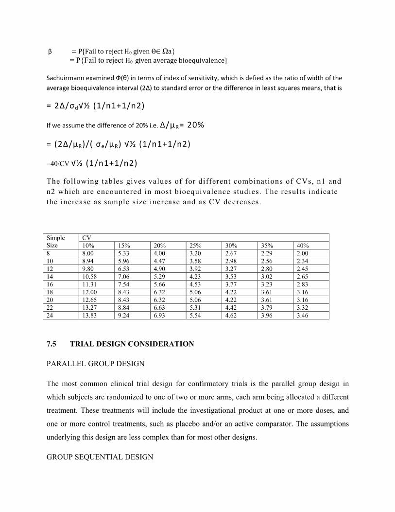
β P Fail to reject H0 given Ωa = PFail to reject H0 given average bioequivalence Sachuirmann examined Ф(θ) in terms of index of sensitivity, which is defied as the ratio of width of the average bioequivalence interval (2Δ) to standard error or the difference in least squares means, that is

= 2Δ/σd√½ (1/n1+1/n2)

If we assume the difference of 20% i.e. Δ/μR= 20%

= (2Δ/μR)/( σe/μR) √½ (1/n1+1/n2)

=40/CV √½ (1/n1+1/n2)

The following tables gives values of for different combinations of CVs, n1 and n2 which are encountered in most bioequivalence studies. The results indicate the increase as sample size increase and as CV decreases.

Simple Size

CV 10% 15% 20% 25% 30% 35% 40%

8 8.00 5.33 4.00 3.20 2.67 2.29 2.00 10 8.94 5.96 4.47 3.58 2.98 2.56 2.34 12 9.80 6.53 4.90 3.92 3.27 2.80 2.45 14 10.58 7.06 5.29 4.23 3.53 3.02 2.65 16 11.31 7.54 5.66 4.53 3.77 3.23 2.83 18 12.00 8.43 6.32 5.06 4.22 3.61 3.16 20 12.65 8.43 6.32 5.06 4.22 3.61 3.16 22 13.27 8.84 6.63 5.31 4.42 3.79 3.32 24 13.83 9.24 6.93 5.54 4.62 3.96 3.46

7.5 TRIAL DESIGN CONSIDERATION

PARALLEL GROUP DESIGN

The most common clinical trial design for confirmatory trials is the parallel group design in

which subjects are randomized to one of two or more arms, each arm being allocated a different

treatment. These treatments will include the investigational product at one or more doses, and

one or more control treatments, such as placebo and/or an active comparator. The assumptions

underlying this design are less complex than for most other designs.

GROUP SEQUENTIAL DESIGN

In this design, a number of subjects are entered and studied. An interim analysis of the data is

then conducted, and if the results are significant or if the treatment groups that is nonsignificant

(statistically) or if the treatment groups are totally alike, then the clinical trial is stopped. If there

is a difference between the two groups that is nonsignificant (statistically), then a second group

of subjects is enrolled, and the same type of randomization is used as was employed for the

original group.

FACTORIAL DESIGN

In a factorial designs two or more treatments are evaluated simultaneously through the of

varying combinations of the treatments. The simplest example of 2x2 factorial design in which

subjects are randomly allocated to one of the four possible combinations of two treatments. A

and B say. These are A alone; B alone; both A and B; neither A nor B. In meny cases this design

is used for the specific purpose of examining the interaction of A and B. The statistical test of

interaction may lack power to detect an interaction if the sample size was calculated based on the

test for main effects. This consideration is important when this design is used for examining the

joint effects of A and B , in particular , if the treatments are likely to be use together.

Another important use of the factorial design is to establish the doseresponse characteristics of

the simultaneous use of treatments C and D, especially when the efficacy of each monotherapy

has been established at some dose in prior trials.

In some cases, the 2x2 design may be used to make efficient use of clinical trial subjects by

evaluating of the two treatments with the same number of subject as would be required to

evaluate the efficacy of either one alone. This strategy has probed to be particularly valuable for

very large mortality trials. The efficiency and validity of this approach depends upon the absence

of interaction between treatment a and B so that the effects of A and B on the primary efficacy

variable follow an additive model, and hence the effect of A is virtually whether or not is it is

additional to the effect of B.

STATISTICAL MODEL AND LINEAR CONTRAST

In a cross over design, because the direct drug effect may be condounded with any carryover

effects, it is important to the remove the carryover effects from the comparison if possible. To

account for these effects, the following statistical model is usually considered. Let ijk be response

(e.g. AUC) of the ith subject in the kth sequence at the jth period.

Where

U = the overall mean:

Sjk = the random effect of the ith subject in the kth sequence.

Where I, 1,2,……….,nk and K = 1,2,……..,g:

Pj = the fixed effect of the jth period, where j =1,…….p and ΣiPi = 0 ;

F(j,k) = the direct fixed effect of the formulation in the kth sequence which is administered at the

jth period, and Σ F(j,k) = 0

C(J-L,K) = the fixed first-order carryover effect of the formulation in the sequence

Which is administered at the (j-1)th period, where (C(o,k) = 0, and Σ C(j-1,k) =0

Eijk = the (within subject) random error in observing Yijk.

It is assumed that (Sjk are independently distributed with mean 0 and variance σ2s

Where t = 1,2,…….L (the number of formulations to be compared) Sjk and eijk are assumed

mutually independent. The estimate of σ2s are used to asses the intrasubject variability for the tth

formulation.

Under the normality assumption, the carryover effects and other dfixed effects, such as the direct

drug effect and the period effect, can be estimated based on the gp means because there are (gp -

1) degree of freedom (df) among these gp means because there are (gp-1) degrees of freedom

(df) among these gp means, which can be decomposed as follows (Joned and Kenward, 2989):

(gp-1) = (p-1)+(g-1)+(p-1)(g-1),

Where (p-1) df are attributed to the period effect, (g-1) df are assigned to the assigned to the

sequence effect, are (p-1)(g-1) df are of particular interest because they preserve the information

related to the direct drug effect and the carryover effects. For example, for a standard 2x2

crossover design, there are 3 df associated with four sequence-by-period means: 1 for the

sequence effect, 1 for the period effect and a for the period effect and a for the sequence-by-

period interaction which is , in fact, the direct drug effect when there are no carryover effects.

A within-subject linear contrast for the kth sequence is defined as a linear combination of .1k,

.2k,…………, and .pk. That is,

Where

Two linear combination of .jks j = 1, 2……..p are said to orthogonal if the sum of the cross

product of the coefficients of the contrasts is 0. In other words, let

Be two linear contrasts, then 11 and l2 areothogonal is

It can be seen that the variance of l involves only the intrasubjuect variability σ2t, t = 1,2,……L.

Thus, statistical inferences for the fixed effects, such as the period effects, the direct drug effects,

and the carryover effects, can be made based on within subject variability using appropriate

linear contrasts of those gp means.

l = cl .1k +c2 .2k + ………cp .pk

Σici = 0

l1 = Σc1j ik and l1 = Σc2j 2k

Σc1j c2j = 0

Subject Sequence Period 1 Washout Period 2

1 TR T 10 days R

2 RT R 10 days T

Where T: Test and R: Reference 2X 2 crossover design

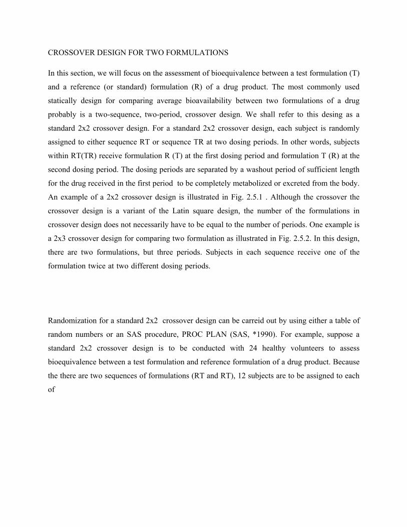
CROSSOVER DESIGN FOR TWO FORMULATIONS

In this section, we will focus on the assessment of bioequivalence between a test formulation (T)

and a reference (or standard) formulation (R) of a drug product. The most commonly used

statically design for comparing average bioavailability between two formulations of a drug

probably is a two-sequence, two-period, crossover design. We shall refer to this desing as a

standard 2x2 crossover design. For a standard 2x2 crossover design, each subject is randomly

assigned to either sequence RT or sequence TR at two dosing periods. In other words, subjects

within RT(TR) receive formulation R (T) at the first dosing period and formulation T (R) at the

second dosing period. The dosing periods are separated by a washout period of sufficient length

for the drug received in the first period to be completely metabolized or excreted from the body.

An example of a 2x2 crossover design is illustrated in Fig. 2.5.1 . Although the crossover the

crossover design is a variant of the Latin square design, the number of the formulations in

crossover design does not necessarily have to be equal to the number of periods. One example is

a 2x3 crossover design for comparing two formulation as illustrated in Fig. 2.5.2. In this design,

there are two formulations, but three periods. Subjects in each sequence receive one of the

formulation twice at two different dosing periods.

Randomization for a standard 2x2 crossover design can be carreid out by using either a table of

random numbers or an SAS procedure, PROC PLAN (SAS, *1990). For example, suppose a

standard 2x2 crossover design is to be conducted with 24 healthy volunteers to assess

bioequivalence between a test formulation and reference formulation of a drug product. Because

the there are two sequences of formulations (RT and RT), 12 subjects are to be assigned to each

of

The two sequence. In other words, one group will receive the second sequence of formulations

(RT) and the other group will receive the second sequence of formulations (TR). Thus, we first

generate a set of random permutations from 1 to 24 using PROCPLAN which follows:

16, 19, 20, 4, 24, 1, 12, 5, 23, 15, 6,

17, 2, 10, 14, 18, 13, 21, 3, 7, 8, 22, 9,

Then subjects are sequentially assigned a number from 1 throgh 24, subjects with numbers in the

first half of the above random order are assigned to the first sequence (RT) and the rest are

assigned to the second seqeuence (TR) (See Table 2.5.1). In practice, a set of randomization code

for more than the total number of subjects planned is usually prepared to account for the possible

replacement of dropout.

For a standard 2x2 crossover design, from Eq. (2.5.1), two responses for the subject in each

sequence are given as :

For each subject a pair of observations is observed at period 1 and period 2. Thus we may

consider a bivariate random vector. i.e. [period 1, period 2] as follows.

Subject Sequence Period‐1 WP Period‐2 WP Period‐3

1 TRR T 10 R 10 R

2 RTT R 10 T 10 T

Where T: Test and R: Reference 2X 3 crossover design WP: Washout Period in Days

Sequence 1 Yi11 = u + si1 + p1 + F1 + ei11 Yi21 = u + Si1 + P2 + F2 + C1 +ei21 Sequence 2 Yi12 = u + Si2 + P1 + F2 + ei12 Yi22 = u + Si2 + P2 + F1 + ei22

Where P1 + P2 = 0, F1 + F2 =0, and C1 +C2 = 0

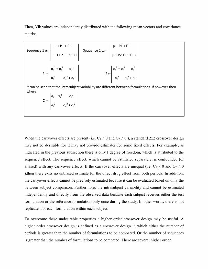
Then, Yik values are independently distributed with the following mean vectors and covariance

matrix:

When the carryover effects are present (i.e. C1 ≠ 0 and C2 ≠ 0 ), a standard 2x2 crossover design

may not be desirable for it may not provide estimates for some fixed effects. For example, as

indicated in the previous subsection there is only I degree of freedom, which is attributed to the

sequence effect. The sequence effect, which cannot be estimated separately, is confounded (or

aliased) with any carryover effects, If the carryover effects are unequal (i.e. C1 ≠ 0 and C2 ≠ 0

),then there exits no unbiased estimate for the direct drug effect from both periods. In addition,

the carryover effects cannot be precisely estimated because it can be evaluated based on only the

between subject comparison. Furthermore, the intrasubject variability and cannot be estimated

independently and directly from the observed data because each subject receives either the test

formulation or the reference formulation only once during the study. In other words, there is not

replicates for each formulation within each subject.

To overcome these undesirable properties a higher order crossover design may be useful. A

higher order crossover design is defined as a crossover design in which either the number of

periods is greater than the number of formulations to be compared. Or the number of sequences

is greater than the number of formulations to be compated. There are several higher order.

µ + P1 + F1 µ + P1 + F1 Sequence 1 α1= Sequence 2 α2 = µ + P2 + F2 + C1 µ + P2 + F1 + C2 σ1

2 + σs2 σ1

2 σ22 + σs

2 σ22

ΣI = Σ2= σs

2 σ22 + σs

2 σs2 σ1

2 + σs2

it can be seen that the intrasubject variability are different between formulations. If however then where σe + σs

2 σs2

ΣI = σs

2 σe2 + σs

2

Crossover designs available in the literature (Kershner and Federer, 1981; Laska and Meinser,

1985 Jones and Kenward 1989). These designs however, have their own advantages and

disadvantages. An in depth discussion can be found in Jones and Kenward (1989).

In the following, we will discuss three commonly used higher order crossover designs which

possess some optimal statistical properties, for comparing average bioavailability between two

formulations. We shall refer to these three designs as design. A design, B, and design C,

respectively Designs, A,B, and C are given in Table 2.5.2. In each of the three designs, the

estimates of the direct drug effect and carryover effects are obatained based on the within subject

linear contrasts.

Table 2.5.1 Randomization Code for a standard 2x2 Crossover Design with 24 subjects

Subject Sequence Formulations

1 1 RT 2 2 TR 3 2 TR 4 1 RT 5 1 RT 6 1 RT 7 2 TR 8 2 TR 9 2 TR

10 2 TR 11 1 RT 12 1 RT 13 2 TR 14 2 TR 15 1 RT 16 1 RT 17 2 TR 18 2 TR 19 1 RT 20 1 RT 21 2 TR 22 2 TR 23 1 RT 24 1 RT

As a result statistical inferences for direct drug effect and carryover effects are based on mainly

the intrasubject variability. For the comparisons of these three designs with the standard 2x2

crossover design, it is helpful to use the following notations. The direct drug effect after

adjustment for the carryover effects is denoted by F/C. Then F simply refers to the unadjusted

direct drug effect. Also V(F) C denotes the variance of the estimate of F/C (i.e., F/C). Table 2.53

gives the variances (in the multiples of ) of the direct drug effect and carryover effects for the

three designs and standard 2x2 crossover design (Jones and Kenward, 1989; Senn. 1993) The

variances of designs, A,B, and C are derived under the assumptions that (a) nk = n for all k (b)

and (c) there is no direct drug by carryover interaction. For designs B and C, the variances.

Optimal Crossover Designs for two formulations

Design A Period Sequence I II 1 T T 2 R R 3 R T 4 T R Design B Period Sequence I II II 1 T R R 2 R T T Design C Period Sequence I II III IV 1 T T R R 2 R R T T 3 R T R T 4 T R T R

Of the direct drug effect adjusted for the carryover effects are the same as the unadjusted direct

drug effect i.e no Carryover effect. This is because the direct drug effect and carryover effects for

designs B and C are estimated by the linear contrasts, which are orthogonal to each other. Note

that an orthogonality of linear contrasts for the direct drug effect and carryover effects implies

that their covariance is zero. In other words, the estimators of the direct drug effect and carryover

effects in designs B and C are not correlated (or independent).

Design A is also known as Balaam’s (Balaam 1968). It is an optimal design in the class of the

crossover designs with two periods and two formulations. This design is formed by adding two

more sequences (sequences 1 and 2) to the standard 2x2 crossover design (sequences 3 and 4)

these two augmented sequences are TT and RR with additional in formulation provided by the

two augmented sequences. Not only can the carryover effects be estimated using the within

subject contrasts, but the intrasubject variability for both test and references formulations can

also to obtained because there are replicates for each formulations within each subject.

Design B is an optimal design in the class of the crossover design with two-sequences, three

periods, and two formulations. It can be obtained by adding an additional period to the standard

2x2 crossover designs. The treatments administered in the third period are the same as those in

the second period. This type of designs is also known as the extended period or extra period

designs. Note that this design is made of a pair of dual sequences TRR and RTT. Two sequences,

the treatment of which are mirror images of each other, are said to be a pair of dual sequences.

As pointed out by Jones and Kenward (1989), the only crossover designs worth considering are

Variance for Designs A,B, and C in Multiples of

Design V(C/F) V(F/C) V(F) Sa _b _c 1.0000 A 4.0000 2.0000 1.0000 B 1.0000 0.7500 0.7500 C 0.3636 0.2500 0.2500

a S is a standard 2x2 crossover design. b V(C/F) = 4 n.

c The direct drug effect is not estimable in the presence of the Carryover effects.

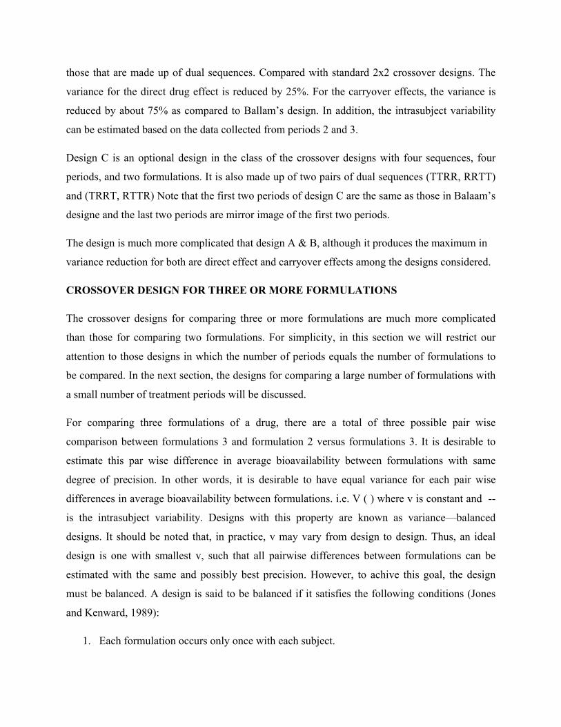
those that are made up of dual sequences. Compared with standard 2x2 crossover designs. The

variance for the direct drug effect is reduced by 25%. For the carryover effects, the variance is

reduced by about 75% as compared to Ballam’s design. In addition, the intrasubject variability

can be estimated based on the data collected from periods 2 and 3.

Design C is an optional design in the class of the crossover designs with four sequences, four

periods, and two formulations. It is also made up of two pairs of dual sequences (TTRR, RRTT)

and (TRRT, RTTR) Note that the first two periods of design C are the same as those in Balaam’s

designe and the last two periods are mirror image of the first two periods.

The design is much more complicated that design A & B, although it produces the maximum in

variance reduction for both are direct effect and carryover effects among the designs considered.

CROSSOVER DESIGN FOR THREE OR MORE FORMULATIONS

The crossover designs for comparing three or more formulations are much more complicated

than those for comparing two formulations. For simplicity, in this section we will restrict our

attention to those designs in which the number of periods equals the number of formulations to

be compared. In the next section, the designs for comparing a large number of formulations with

a small number of treatment periods will be discussed.

For comparing three formulations of a drug, there are a total of three possible pair wise

comparison between formulations 3 and formulation 2 versus formulations 3. It is desirable to

estimate this par wise difference in average bioavailability between formulations with same

degree of precision. In other words, it is desirable to have equal variance for each pair wise

differences in average bioavailability between formulations. i.e. V ( ) where v is constant and --

is the intrasubject variability. Designs with this property are known as variance—balanced

designs. It should be noted that, in practice, v may vary from design to design. Thus, an ideal

design is one with smallest v, such that all pairwise differences between formulations can be

estimated with the same and possibly best precision. However, to achive this goal, the design

must be balanced. A design is said to be balanced if it satisfies the following conditions (Jones

and Kenward, 1989):

1. Each formulation occurs only once with each subject.

2. Each formulation occurs the same number of timesin each period.

3. The number of subjects who receive formulation I in some period followed by

formulation j in the next period is the same for all 1=j

R is the reference information T1, T2 & T3 are test formulation 1,2 & 3 respectively.

Orthogonal Latin Squares for t =3 and 4 Three formulations (t =3) period Sequence I II III

1 Ra T1 T2 2 T1 T2 R 3 T2 R T1 4 R T2 T1 5 T1 R T2 6 T2 T1 R

Four Formulations (t =4)

Period Sequence I II III IV 1 R4 T1 T2 T3 2 T1 R T3 T2 3 T2 ` T3 R T1 4 T3 T2 T1 R 5 R T3 T1 T2 6 T1 T2 R T3 7 T2 T1 T3 R 8 T3 R T2 T1 9 R T2 T3 T1 10 T1 T3 T2 R 11 T2 R T1 T3

12 T3 T1 R T2

Under the constraints of the number of periods (p) being equal to the number of formulation (1),

balance can be achieved by using a complete set of “orthogonal Latin Squares” (John, 1971;

Jones and Kenward, 1989). However if, p=1 a complete set of orthogonal Latin Squares consists

of t(t-1) sequence except for t=4 are presented in Table 2.5.4 As a result, when the number of

formulations to be compared is large, more sequences and consequently more subjects are

required. This, however, may not be practical use.

A more pratical design has been proposed to Williams (1949). We shall refer to this as a William

Design. A William Design possesses balance properlty and requires fewer sequences and

periods. The algorithm for constructing a William Design with t period and t formulation is

summarized in the following steps (Jones and Kenwardm, 1989).

1. Numebr of formulations from 1,2,3,….

2. Start with a txt standard Latin Square. In this square, the formulations in the ith row are

given by I, I+1, …..t, 1,2,……I-1,

3. Obtain a mirror imagae of the standard Latin Square.

4. Interlace each row of the standared Latin Square with the corresponding mirror image to

obtain a tx2t arrangement

5. Since the 2 x 2t arrangement down to the idle to yield two t x t squares. The columns of

each t x t squares correspond to the period and the rows are the sequences. The number

within the square are the formulations.

6. It is even, choose any one of the two t x t squares. If t is odd, use both squares.

In the following, to illustrate the use of this alogithm as an example, we will construct a William

design with t =4 (one reference and three test formulations) by following the above steps.

Denote the reference formulation by 1 and test formulation 1, 2 and 3 by 2, 3, and 4. A 4x4 standard Latin square is given as 1 2 3 4 2 3 4 1 3 4 1 2 4 1 2 3 The minor image of the 4x4 standard Latin square is then given by 4 3 2 1 1 4 3 2 2 1 4 3 3 2 1 4 The 4x8 arrangement after interlacing the 4x4 standard Latin square with its mirror image is 1 4 2 3 | 3 2 4 1 2 1 3 4 | 4 3 1 2 3 2 4 1 | 1 4 2 3 4 3 1 2 | 2 1 3 4 The 4x4 squares obtained by slicing the 4x8 arrangement are Period Square Sequence I II III IV 1 1 1 4 2 3 2 2 1 3 4 3 3 2 4 1 4 4 3 1 2 2 1 3 2 4 1 2 4 3 1 2 3 1 4 2 3 4 2 1 3 4

Because t =4, we can choose either square 1 or square 2. The resultant Williams designs from

square 1 is given in Table 2.5.5 by replacing 1,2,3,4, with R, T1, T2 and T3.

From the above example, it can be seen that a Williams design requires only 4 sequences to

achieve the property of “variance-balanced,” whereas a complete set of 4 x 4 orthogonal Latin

squires 12 sequences. A William design with t =3 and 5 constructed using the above algorithm

are also given.

THE BALANACED INCOMPLETE BLOCK DESIGN

The comparing three or more formulations of a drug product, a complete crossover design may

not be practical interest for the following reasons (Westlake, 1973):

1. If the number of formulations to be compared is large, the study may be too time-

consuming, since t formuations require t -1 washout periods.

2. It may not be desirable to draw many blood samples for each subject owing to medical

concerns.

3. Moreover, a subject is more likely to drop out when he or she is required to return

frequently for tests.

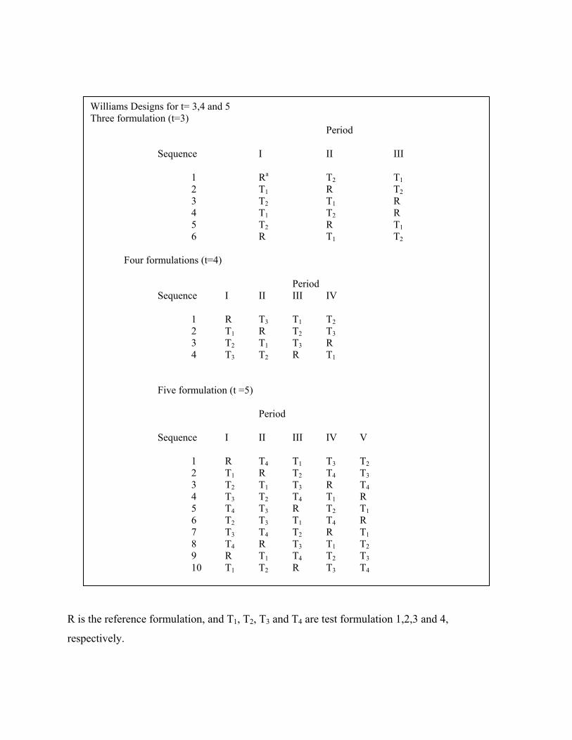
R is the reference formulation, and T1, T2, T3 and T4 are test formulation 1,2,3 and 4,

respectively.

Williams Designs for t= 3,4 and 5 Three formulation (t=3) Period Sequence I II III 1 Ra T2 T1 2 T1 R T2 3 T2 T1 R 4 T1 T2 R 5 T2 R T1 6 R T1 T2 Four formulations (t=4) Period Sequence I II III IV 1 R T3 T1 T2 2 T1 R T2 T3 3 T2 T1 T3 R 4 T3 T2 R T1

Five formulation (t =5)

Period Sequence I II III IV V 1 R T4 T1 T3 T2 2 T1 R T2 T4 T3 3 T2 T1 T3 R T4 4 T3 T2 T4 T1 R 5 T4 T3 R T2 T1 6 T2 T3 T1 T4 R 7 T3 T4 T2 R T1 8 T4 R T3 T1 T2 9 R T1 T4 T2 T3 10 T1 T2 R T3 T4

These considerations suggest that one should keep the number of formulations that a subject

receives as small as possible when planning a bioavailability study. For this, a randomized

incomplete block design may be useful. An incomplete block design is a randomized block

design in which not all formulation present in the block is less than the number of formulations

to be compared. For an incomplete block design the blocks and formulations are not orthogonal

to each other; that is, the black effects and formulations effects may not be estimated separately.

When an incomplete block design is used, it is recommended that the formulation in each block

randomly assigned in a balanced way so that the design will possess more optimal statistical

properties. We shall refer to such a design as a balanced incomplete block design. A balanced

incomplete block design is an incomplete block design in which any two formulations appear

together an equal number of times. The advantages of using a balanced incomplete block design,

rather than an incomplete design, are given as follows:

1. The difference in average bioavailability between the effects of any two formulations can

always be estimated with the same degree of precision.

2. The analysis is simple in spite of the nonorthogonality provided that the balance is

preserved.

3. Unbiased estimateds of formulation effects are available.

Suppose that there is t formulation to be compared and each subject can only receive exactly p

formulations (t >p). A balanced incomplete block design may be constructed by taking C (t,p),

the combinations of p out of t formulations, and assigning a different combination of

formulations to each subject. However, to minimize the period effect, it is preferable to assign

the formulation in such a way that the design is balanced over period (i.e. each formulation

appears the same number of formulations is even (i.e., t = 2n) and p =2, the number of blacks

(sequences) required is g = 2n(2n -1). On the other hand, if the number of formulations is odd

(i.e. t = 2n + 1) and p = 2, then g = (2n + 1) n. Some example for balanced incomplete block

design are given in Table 2.6.1 and 2.6.2. Table 2.6.1. given example for p=2, the first six blocks

are requried for a balanced incomplete block design. However, to ensure the balance over period,

an additional six blocks (7 through 12) are needed. For t =5, Table 2.6.2. lists examples for a

balanced incomplete block design with p= 2,3, and 4. A balanced incomplete block design ofr p

= 3 is the complementary part of that balanced incomplete block design for p=3 is the

complementary part of that balanced incomplete block design for p =2. The design for p=4 can

be constructed by deleting each formulation in turn to obtain five blocks seccessively.

For t >5, several methods for constructing balanced incomplete block designs are available.

Among these, the easiest way is probably the method of cyclic substition. For this method to

work, we first choose an appropriate initial block. The other can be obtained successively by

changing.

Balancedd Incomplete Block Designs for t = 4 with p =2 and 3 Each sequence receives two formulations (p=2) Period Sequence I II 1 Rb T1 2 T1 T2 3 T2 T3 4 T3 R 5 R T2 6 T1 T3 7 T3 T1 8 T2 R 9 R T3 10 T3 T2 11 T2 T1 12 T1 R Each sequence receives three formulations (p=3) Period Sequence I II III 1 T1 T2 T3 2 T2 T3 R 3 T3 R T1 4 R T1 T2

a A sequence (0r block) may reperesent a subject or a groups of homogeneous subjects. b R is the reference formulation, 1,2, and 3, respectively.

Formulations A to B, B to C,……, and so on in each block. For example, for t =6 and p =3, if we

start with (A, B, D), then the second block is (B, C, E), and the trird block is (C,D,F), and so on.

Note that a balanced incomplete block design is, in fact, a special case of variance-balanced

design, which will be discussed in Chap. 10. For an incomplete block design, balance may be

achieved with fewer than C (t,p) blocks. Such designs are known as partially balanced

incomplete block designs. The analysis os these designs, however, are complicated and, hence,

of little paractical interest. More details on balanced incomplete block designs and partially

balanced incomplete block designs can be found in Fisher and Yates (1953), Bose et al. (1954),

Cochran and Cox (1957), and John (1971).

Balanced Incomplete Block Designs for t = 5 with p = 2,3, and 4 Each sequence received two and three formulations P=2 p=2 Period period Sequence a I II Sequence I II III 1 Rb T1 1 T2 T3 T4 2 T1 T2 2 T3 T4 R 3 T2 T3 3 T4 R T1 4 T3 T4 4 R T1 T2 5 T4 T1 5 T1 T2 T3 6 R T2 6 T1 T3 T4 7 T2 T4 7 T3 R T1 8 T4 T1 8 R T2 T3 9 T1 T3 9 T2 T= R 10 T3 R 10 T4 T1 T2 Each sequence receives four formulations (p=4) Period Sequence I II III IV 1 T1 T2 T3 T4 2 T2 T3 T4 R 3 T3 T4 R T1 4 T4 R T1 T2 5 R T1 T2 T3

A Sequence (or block) may represent a subject or a group of homogeneous subjects.

R is the reference formulation and T1, T2, T3 and T4, are test formulations 1,2,3, and 4

respectively.

7.6 THE SELECTION OF DESIGN

In previous sections, we briefly discussed three basic statistical designs, the parallel design, the

crossover design, and the balanced incomplete block design for bioavailability and

bioequivalence studies. Each of these has its own advantages and drawbacks under different

circumstances. How to select an appropriate design when planning a bioavailability study is an

important question. The answer to this question depends on many factors that are summarized as

follows:

1. The number of formulations to be compared

2. The characteristics of the drug and tis disposition

3. The study objective

4. The availability of subjects

5. The inter and intrasubject variabilities

6. The duration of the study or the number of periods allowed

7. The cost of adding a subject releative to that of addign one periosed.

8. Dropout rates

For example, if the intrasubject variability is the same as or larger than the intersubject

variability, the inference on the difference in average bioavailibiliy would be the same regardless

of which design is used. Actually, a crossover design in this situation would be a poor choice,

because blocking results in the loss of the some degrees of freedom and will actually lead to a

wider confidence intereval on the difference between formulations.

If a bioavailability and and bioequivalence study compares more than three formulations, a

crossover design may not be approprite. The reasons, as indicated in Sec. 2.6, are (a) it may be

too-consuming to complete the study because a washout is required between treatment periods;

(b) it may not be desirable to draw many blood samples for each subjects owing to medical

concerns; and (c) too many periods may increase the number of dropouts. Here, a balanced

incomplete block design is preferred. However, if we compare several test formulations with a

reference formulation, the within-subject comparison is not reliable, at the subjects in some

sequences may not receive the reference formulation.

If the drug has a very long half-life, or it possesses a potential toxicity, or bioequivalence must

be established by clinical endpoint because some drugs do not work through systemic absorption,

then a parallel design may be a possible choice. With this design, the study avoids a possible

cumulative toxicity from the effects from one treatment period to the next. In addition, the study

can be completed quickly. However, the drawback is that the comparison of average

bioavailability is made based on the intersubject variability. If the intersubject variability is large

relative to the intrasubject variability, the statistical inference on the difference in average

bioavailability between formulations is underliable. Even if the intersubject variability is

relatively small, a parallel design may still require more subjects to reach the same degree of

precision achieved by a crossover design.

In practice, a crossover design, which can remove the intersubject variability from the

comparison of bioavailability between formulations, is often considered to be the design of

choice if the number of formulations to be compared is small say no more than three. If the

length of washout is along enough to eliminate the residual effects, a crossover design may be

useful for the assessment of intresubject variability, provided that the cost for adding one period

is comparable with that of adding a subject.

In summary, to choose an appropriate design for a bioavailability study is an important issue in

the development of a sutdy protocol. The selected design may affect the data analysis, the

interpretation of the results, and the determination of bioequivalence between formulations.

Thus, all factors listed in the above should be carefully evaluated before an appropriate design.

SWITCHING BETWEEN SUPERIORITY AND NON-INFERIORITY

A number of recent applications have led to CAMP discussions concerning the interpretation of

superiority, non-interiority and equivalence trials. These issues are covered in ICH E9 (statistical

Principles for Clinical Trials). There is further relevant material in the CPMP Note for Guidance

on the Investigation of Bioavailability and Bioequivalence. However, the guidelines do not

address some specific difficulties that have arisen in practice. In borad terms, these difficulties

relate to switching from one design objective to another at the time of analysis.

The type of trials in question are those designed to comapre a new product with an active

comparator. The objective may be to demonstrate:

• The superiority of the new product

• The non-inferiority of the new product or

• The equivalence of the two products.

When the resutl of trial become available, they may suggest an alternative interpretation. Thus

the results of a superiority trial may only appear to be sufficient to support non-inferiority while

the results of a non-inferiority trial may appear to support superiority. Alternatively, the results

of an equivalence trial may appear to support a tighter range of equivalence.

A satisfactory approach to this subject requires an understanding of confidence intervals and the

manner in which they capture the results of the trial and indicate the conclusions that can be

drawn from them. Such an understading also lead to an appreciation of why power calculations

are of relatively little interest when a trial is complete.

For, simplicity, this paper address the issues of superiority, non-inferiority and equivalence from

the perspective of an efficacy trial with a single primary vairable. Some comments on other

situations are made in Section VI. It is assumed throughout this document that switching the

objective of a trial does not lead to any change in the selection or definition of the primary

variable.

TRIAL OBJECTIVES

SUPERIORITY TRIAL

A superiority trial is designed to detect a difference between treatments. The first step of the

analysis is usually a test of statistical significance to evaluate whether the results of the trial are

consistent with the assumption of there being to difference in the clinical effect of the two

treatments. In a trial of good quality, the degree of statistical significance (p-value) indicates the

probability that the observed – or a larger one – could have arisen by chance assuming that no

difference really existed. The smaller this probability is the more implausible is the assumption

that there really is no difference between the treatments.

Once it is accepted that the assumption of “no difference” is untenable, it then becomes

important to estimate the size of the difference in order to assess whether the effect is clinically

relevant. This has two aspect. First these is the best estimate of the size of the difference between

treatmenets (points estimate). For normally distributed date this is usually taken as the observed

difference between the difference between the mean values of each. Next, there is the range of

the value of the true difference that are plausible in the light of results of the trial (confidence

interval) it is clear that this range should not include zero since the possibility of a zero

difference has already been rejected as unreasonable. The method of cnstructing confidence

intervals generally ensures that this is so, provided a corresponds to the choice of significance

test. Thus the following two statements equivalent:

The two sided 95% confidence interval for the difference between the menas excludes zero.l

The two means are statistically significantly difference that the 5% level (p<0,.05) two sided.

The above text addresses the situation where the difference between two mean values is the

statistics are used for the evaluation of differences between treatments, for each example the odd

ratio for proportions or the ratio of geometric menas in bio-equivalence studies. (The latter arises

from the logarithm tic used for bio-availability data). In such cases the same principles apply but

no difference may be represented by a value other than zero a value of 1 in both the examples

quoted here. In these cases it is the position of the confidence interval for the test statistics

relative to this ‘no difference’ value that is of interest.

When significance tests are carried out in practice numerical values of probabilities are usually

quoted out in practice, precise numerical values of probabilities, are usually quoted, for example

p=0.032, because this is more informative than <0.05. This allows judgment to be based more

precisely on the extent of the disagreement between the null hypothesis and the observed dat

rather than on the approximations implied by using cut off points of 0.05, 0.01 and 0.001.

However, confidence intervals have to be associated with a specific value (coverage probability)

and this is nealy taken as 95% (0.95). when a difference is statistically significant at a more

extreme level, e.g. p = 0.002, the two sided 95% confidence interval will exclude zero by a wider

margin. Figure 1 illustrates this point.

Whether the observed difference is indeed clinically relevant is matter of judgment. In contrast to

an equivalent or non-inferiority trial where clinical relevance requires separate consideration ; a

significant difference may not be in superiority trial can not be assumed to provide a suitable

value.

Note that in above figure, and throughout the rest of the document, it is assumed that values to

the right of zero correspond to better response on the treatment so that value to the left is worse.

i.e. better on the control treatment.

EQUIVALENCE TRIAL

An equivalence trial is designed to confirm the absence of a meaningful difference between

treatments. In this case it is more informative to conduct the analysis by means of the calculation

and examination of the confidence interval throughout, there are closely related methods using

significance test procedures. A margin of clinical equivalence ( ) is chosen by defining the

largest difference that is clinically acceptable, so that a difference bigger than this would matter

in practice. There are well recognized difficulties associated with this task which will not be

discussed in any detail here. If the two treatments are to be declared equivalent. Then the two-

sided 95% confidence interval – which defines the range of plausible difference between the two

treatments – should lie entirely within the interval – to + . See figure 2. These are situations in

which the equivalence margins may be chosen asymmetrically with respect to zero.

In the case of bioequivalence studies a coverage probability of 90% for the confidence interval

has become the accepted standard when evaluating whether the average values of the

pharmacokinetic parameters of two formulations are sufficiently close.

Clinical equivalence trials, with two-sided 95% confidence intervals, may be carried out when

conventional bio-equivalence trials are impossible, for example in the case of a generic inhaled

or topically applied product.

NON-INFERIORITY TRIAL

In Phase III drug development, non-inferiority trials are more common then equivalence trials. In

these we wish to show that a new treatment is no less effective than an existing treatment – it

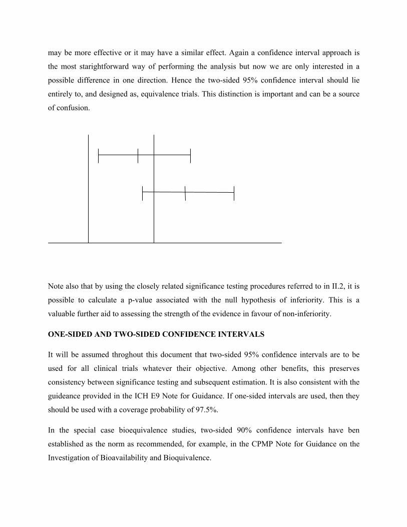
may be more effective or it may have a similar effect. Again a confidence interval approach is

the most starightforward way of performing the analysis but now we are only interested in a

possible difference in one direction. Hence the two-sided 95% confidence interval should lie

entirely to, and designed as, equivalence trials. This distinction is important and can be a source

of confusion.

Note also that by using the closely related significance testing procedures referred to in II.2, it is

possible to calculate a p-value associated with the null hypothesis of inferiority. This is a

valuable further aid to assessing the strength of the evidence in favour of non-inferiority.

ONE-SIDED AND TWO-SIDED CONFIDENCE INTERVALS

It will be assumed throghout this document that two-sided 95% confidence intervals are to be

used for all clinical trials whatever their objective. Among other benefits, this preserves

consistency between significance testing and subsequent estimation. It is also consistent with the

guideance provided in the ICH E9 Note for Guidance. If one-sided intervals are used, then they

should be used with a coverage probability of 97.5%.

In the special case bioequivalence studies, two-sided 90% confidence intervals have ben

established as the norm as recommended, for example, in the CPMP Note for Guidance on the

Investigation of Bioavailability and Bioquivalence.

7.7 ANALYSIS OF BIOEQUIVALENCE/BIOAVAILABILITY TRIAL DATA

The statistical issue associated with the analysis of bioavailability/bioequivalence studies that

whether two formulation of drug have been shown to be equivalent with respect to average

bioavailability in the population. ‘Bioavailability’, in this context, is to be characterized by one

or more blood concentration profile variables, such as under the blood concentration-time curve

(AUC), maximum concentration (Cmxa) etc. and possibly by urinary excretion variables as well.

PROBLEM

Suppose we have a bioavailability /bioequivalence study in which a test product T and a

reference product R are administered. The reference product could be an innovator’s product and

the test product a potential generic substitute manufactured by a different firm. Let µR the

average bioavailability of the reference product. The structure of the statistical hypothesi will be

For untransformed data

H0:µ1-µR < = θL or µT-µR >= θU Vs.

Ha : θL < µT-µR < θU.

For In-transformed data

Ln-transformed pk responses AUC0-t, AUC0-∞ and Cmax:

H0:µ1 / µR < = δL or µT/µR >= δU Vs.

H0: δL < µT/µR < δU .

Where µT,µR are least squares mean for test and reference, θL and θU are 20% of reference mean

µR, δL = exp(θL) and δU =exp(θU).

METHOD

These methods are applicable to statistical analysis of pharmacokinetic parameters obtained from

balanced or unbalanced two way cross over bioequivalence study design ofr untransformed and

log transformed data. Following procedure has been made in accordance to the Guidance issued

by US FDA entitled “Statistical Procedures For Bioequivalence Studies Using a Standard Two-

Treatment Crossover Design” – Guideance! This procedure is to be modified as and when above

procedure is modified by US FDA.

Male logarithimic transformation to base e (natural logarithm) of pharmacokinetic parameters

Perform statistical analysis for both untransformed and In-transformed set of observations.

Use PROC GLM to perform analysis of variance (ANOVA) with following specifications:

Dependent or response variables: AUC0-t, AUC0-∞ and Cmax:

CLASS Statement (Main effects): Sequence, Subjects, Period, Treatment. Model Statement

(Independent variables): Sequence, Subject (Sequence), Period and Treatment. (Attachment No.

2)

Use TEST statement to compute sequence effect and is being tested using the Subject (Sequence)

mean square error from the ANOVA as an error term. (Attachment No.2)

Perform PROC GLM with :

LSMEANS statement to calculate least square means for treatments.

CONTRAST statement in to assess treatment effect.

ESTIMATE statement to estimate differences between treatment means and the standard error

associated with these differences.

Construct 90% confidence interval for testing interval hypothesis described in the problem. Use

α = 0.05 and degrees of freedom (df) generated from ANOVA for calculating t-value.

Untransformed data : 100*(LSMt±t(df,0.05)*Set-r) / LSMr

In-transformed data : 100*e(LSMt – LSMr ±t(df,0.05)*SEt –r)

Where

t(df,0.05) is the Student’s t-distribution with df degrees of freedom and right-tail area of α.

SEt-r is the standard error of the adjusted difference between the formulation means as computed

by the ESTIMATE statement of the SAS®GLM procedure.

Calculate ratio of least square means of test reference formulation for untransformed and In-

transformed pharmacokinetic parameters using the formula:

Untransformed data : 100*(LSMt/LSMr) In-transformed data : 100*e(LSMt/LSMr)

Where

LSM(t,r) is the least-squares mean of the test or reference formulation, as computed by the

LSMEANS statement of the SAS® GLM procedure.

Calculate intrasubject variability using RMSE computed by PROC GLM for untransformed and

In-transformed pharmacokinetic parameters as follows:

Untransformed data : 100* √(e(MSE)-1)

Where

MSE is the mean square error from the analysis of variance.

Overall mean is combined mean value for each parameter, as calculated by the SAS® GLM

procedure.

Calculate power of test to detect as large or greater than 20% of reference mean.

Untransformed data : 100*Prob0.2*LSMr/SEt-r) – t(df,0.025) > tdf

Ln-transformed data : 100*Prob In(1.25)/SEt-r –t(df, 0.025) >tdf

Calculate sample size in total using intrasubject variability generated from In-transformed data

assuming 10% difference between products using the following formula:

n >2*[tα, 2n-n + tβ, 2n-2]2 [CV/(V-δ)]2 where

n = number of subjects per sequence

t = appropriate value from t-distribution

α = significance level (usually 0.10)

1- β = power (usually 0.8)

δ = difference between product

CV = coefficient of variation

V = bioequivalence limit.

The NPARIWAY is used to assess the pharmacokinetic parameter Tmax. Perform Wilcoxon Sign

Rank Sum Test in NPARIWAY to compare the mean scores of test and reference formulations.

Wilcoxon-Mann-Whitney Two One-Sided Tests Procedure may be performed to determine

nonparametric confidence interval for Tmax as this variable being discrete variable.

7.8 ANALYSIS OF CLINICAL TRIAL DATA

The statistical hypotheses to be tested can be structured as follows:

STUPERIORITY TRIAL

H0 : µID = µCD Vs. Ha:µID ≠ µCD

EQUIVALENCE TRIAL

H0: µID - µCD < = θL or µID - µCD >= θU Vs.

Ha : θL < µID - µCD <θU.

θL and θU are the lower equivalence margin and the upper equivalence margin as defined in the

protocol.

NON-INFERIORITY TRIAL

H0: µID - µCD = θL Vs. Ha : H0: µID - µCD > θL

θL is the lower equivalence margin as defined in the protocol.

µID and µCD are least squares mean for investigational and control drug. The statistical model to

be used for the estimation and testing of treatment effects should be described in the protocol.

The main treatment effect should be investigated using the following statistical model with the

assumptions described below:

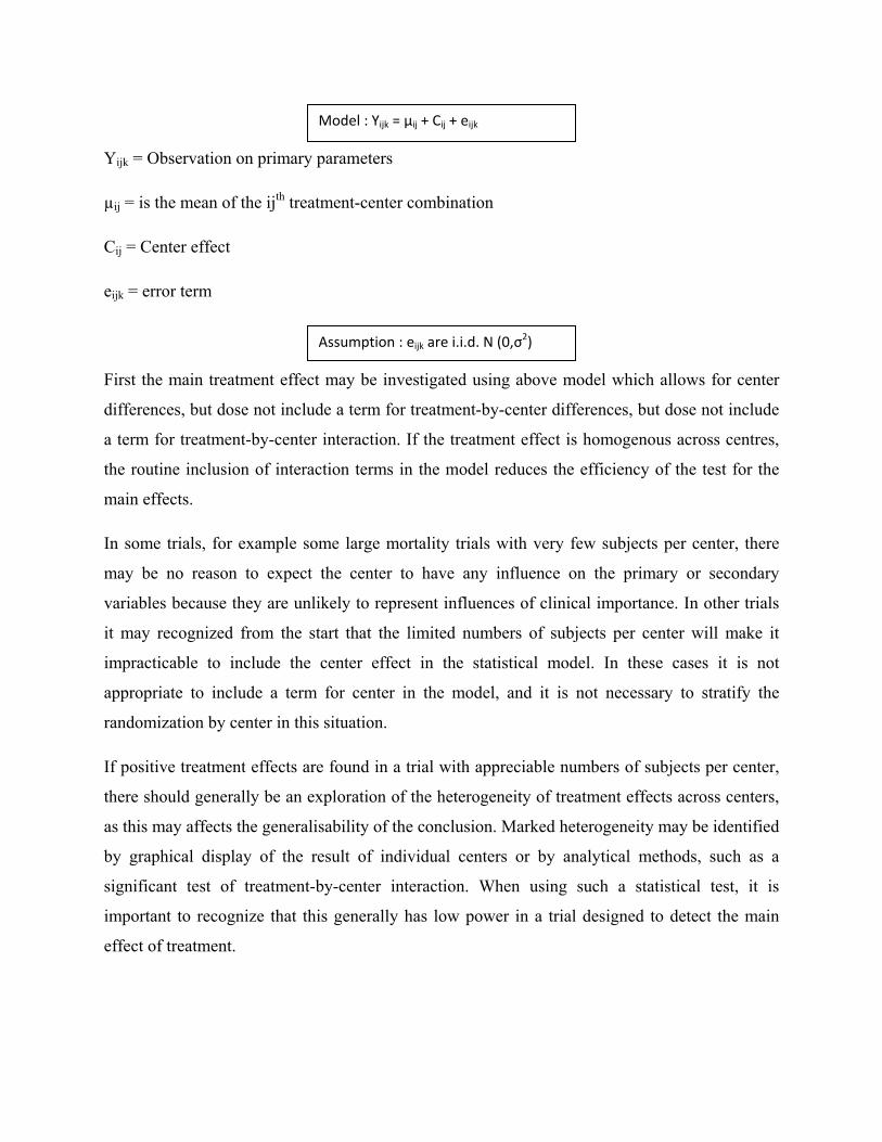
Yijk = Observation on primary parameters

µij = is the mean of the ijth treatment-center combination

Cij = Center effect

eijk = error term

First the main treatment effect may be investigated using above model which allows for center

differences, but dose not include a term for treatment-by-center differences, but dose not include

a term for treatment-by-center interaction. If the treatment effect is homogenous across centres,

the routine inclusion of interaction terms in the model reduces the efficiency of the test for the

main effects.

In some trials, for example some large mortality trials with very few subjects per center, there

may be no reason to expect the center to have any influence on the primary or secondary

variables because they are unlikely to represent influences of clinical importance. In other trials

it may recognized from the start that the limited numbers of subjects per center will make it

impracticable to include the center effect in the statistical model. In these cases it is not

appropriate to include a term for center in the model, and it is not necessary to stratify the

randomization by center in this situation.

If positive treatment effects are found in a trial with appreciable numbers of subjects per center,

there should generally be an exploration of the heterogeneity of treatment effects across centers,

as this may affects the generalisability of the conclusion. Marked heterogeneity may be identified

by graphical display of the result of individual centers or by analytical methods, such as a

significant test of treatment-by-center interaction. When using such a statistical test, it is

important to recognize that this generally has low power in a trial designed to detect the main

effect of treatment.

Model : Yijk = µij + Cij + eijk

Assumption : eijk are i.i.d. N (0,σ2)

Mixed model may also be used to explore the heterogeneity of the treatment effect. These

models consider center and treatment-by-center effects to be random, and are especially relevant

when the number of sites is large.

Construct two-sided 95% confidence interval for testing interval hypotheses for superiority and

equivalence trials and one-sided 95% confidence interval for testing interval hypothesis for non-

inferiority trial. Use the following criteria to conclude whether the investigational drug is

superior or equivalence or non-inferior as defined in the protocol:

Conclude superiority of investigational drug over control drug if two-sided 95% confidence

interval for the difference between means excludes zero.

Conclude equivalence of investigational drug as compare to control drug if two-sided 95%

confidence interval for the difference between means lie entirely within clinically acceptable

range as defined in the protocol.

Conclude non-inferiority of investigational drug as compare to control drug if one-sided 95%

confidence interval for the difference between means lie entirely right of the clinically acceptable

value as defined in the protocol.