chapter 920 data simulator - ncss

PASS Sample Size Software NCSS.com

920-1 © NCSS, LLC. All Rights Reserved.

Chapter 920

Data Simulator

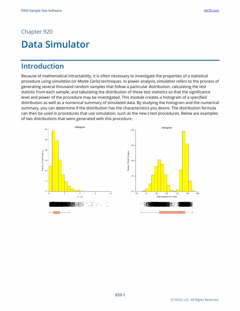
Introduction Because of mathematical intractability, it is often necessary to investigate the properties of a statistical procedure using simulation (or Monte Carlo) techniques. In power analysis, simulation refers to the process of generating several thousand random samples that follow a particular distribution, calculating the test statistic from each sample, and tabulating the distribution of these test statistics so that the significance level and power of the procedure may be investigated. This module creates a histogram of a specified distribution as well as a numerical summary of simulated data. By studying the histogram and the numerical summary, you can determine if the distribution has the characteristics you desire. The distribution formula can then be used in procedures that use simulation, such as the new t-test procedures. Below are examples of two distributions that were generated with this procedure.

http://www.ncss.com/

PASS Sample Size Software NCSS.com Data Simulator


Technical Details This section provides details on each of the distributions that may be generated using this procedure.

Beta Distribution The beta distribution is given by the density function

𝑓𝑓(𝑥𝑥) =𝛤𝛤(A + B)𝛤𝛤(𝐴𝐴)Γ(𝐵𝐵)

�𝑥𝑥 − 𝐶𝐶𝐷𝐷 − 𝐶𝐶

�𝐴𝐴−1

�1 −𝑥𝑥 − 𝐶𝐶𝐷𝐷 − 𝐶𝐶

�𝐵𝐵−1

, 𝐴𝐴,𝐵𝐵 > 0,𝐶𝐶 ≤ 𝑥𝑥 ≤ 𝐷𝐷

where A and B are shape parameters, C is the minimum, and D is the maximum. In statistical theory, C and D are usually zero and one, respectively, but the more general formulation used here is more convenient for simulation work. A beta random variable may be specified using either of two parameterizations: Beta(A, B, C, D) or BetaMS(Mean, SD, C, D). If BetaMS(..) is used, the program solves for the values of A and B from the Mean and SD using the following relationships

𝑀𝑀𝑀𝑀𝑀𝑀𝑀𝑀 = (𝐷𝐷 − 𝐶𝐶) �𝐴𝐴

𝐴𝐴 + 𝐵𝐵� + 𝐶𝐶

𝑆𝑆𝐷𝐷 = �(𝐷𝐷 − 𝐶𝐶)2

(𝐴𝐴 + 𝐵𝐵)2 �𝐴𝐴𝐵𝐵

𝐴𝐴 + 𝐵𝐵 + 1�

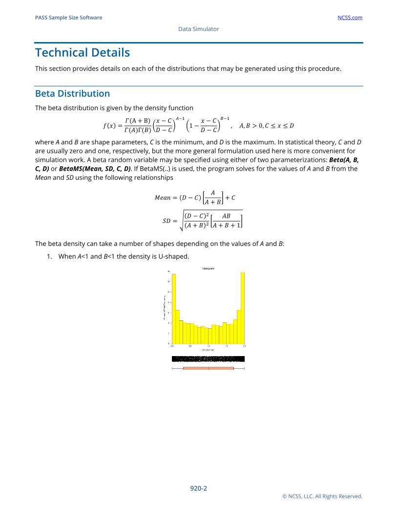
The beta density can take a number of shapes depending on the values of A and B:

1. When A<1 and B<1 the density is U-shaped.




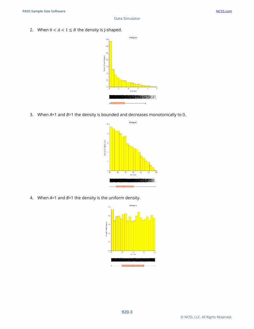
2. When 0 < 𝐴𝐴 < 1 ≤ 𝐵𝐵 the density is J-shaped.

3. When A=1 and B>1 the density is bounded and decreases monotonically to 0.

4. When A=1 and B=1 the density is the uniform density.




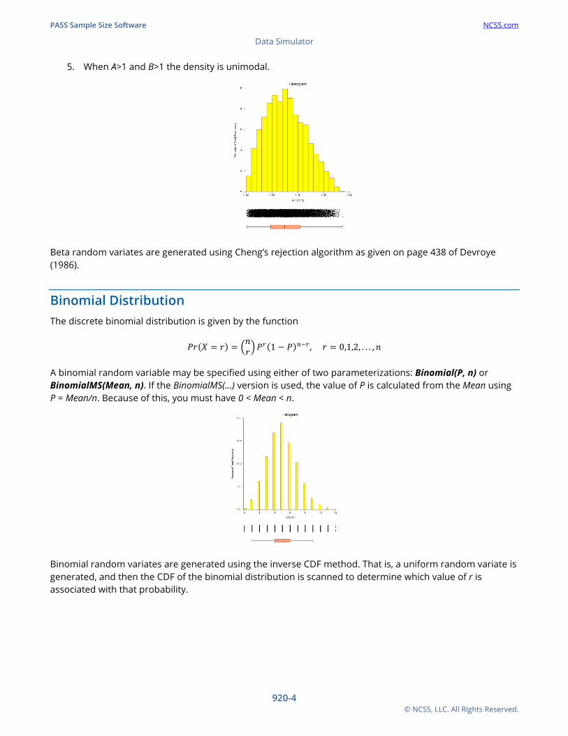
5. When A>1 and B>1 the density is unimodal.

Beta random variates are generated using Cheng’s rejection algorithm as given on page 438 of Devroye (1986).

Binomial Distribution The discrete binomial distribution is given by the function

𝑃𝑃𝑃𝑃(𝑋𝑋 = 𝑃𝑃) = �𝑀𝑀𝑃𝑃�𝑃𝑃𝑟𝑟(1 − 𝑃𝑃)𝑛𝑛−𝑟𝑟 , 𝑃𝑃 = 0,1,2, . . . ,𝑀𝑀

A binomial random variable may be specified using either of two parameterizations: Binomial(P, n) or BinomialMS(Mean, n). If the BinomialMS(…) version is used, the value of P is calculated from the Mean using P = Mean/n. Because of this, you must have 0 < Mean < n.

Binomial random variates are generated using the inverse CDF method. That is, a uniform random variate is generated, and then the CDF of the binomial distribution is scanned to determine which value of r is associated with that probability.




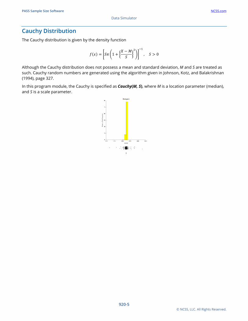
Cauchy Distribution The Cauchy distribution is given by the density function

𝑓𝑓(𝑥𝑥) = �𝑆𝑆𝑆𝑆 �1 + �𝑋𝑋 − 𝑀𝑀𝑆𝑆

�2

��−1

, 𝑆𝑆 > 0

Although the Cauchy distribution does not possess a mean and standard deviation, M and S are treated as such. Cauchy random numbers are generated using the algorithm given in Johnson, Kotz, and Balakrishnan (1994), page 327.

In this program module, the Cauchy is specified as Cauchy(M, S), where M is a location parameter (median), and S is a scale parameter.




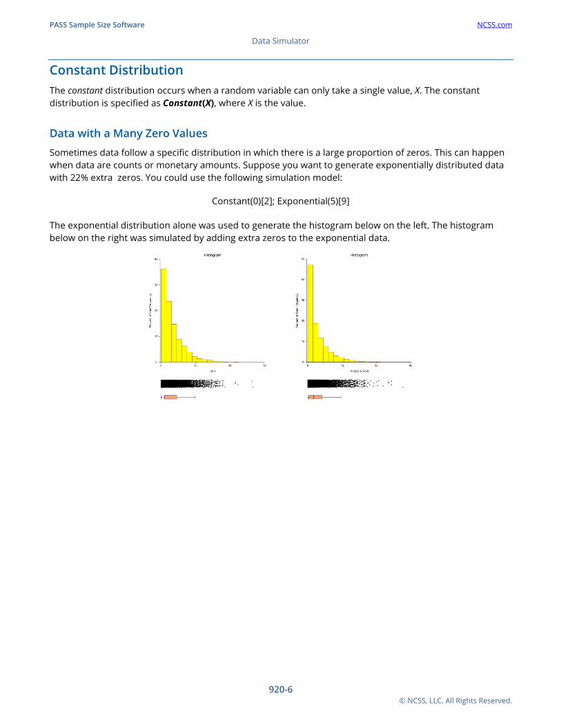
Constant Distribution The constant distribution occurs when a random variable can only take a single value, X. The constant distribution is specified as Constant(X), where X is the value.

Data with a Many Zero Values

Sometimes data follow a specific distribution in which there is a large proportion of zeros. This can happen when data are counts or monetary amounts. Suppose you want to generate exponentially distributed data with 22% extra zeros. You could use the following simulation model:

Constant(0)[2]; Exponential(5)[9]

The exponential distribution alone was used to generate the histogram below on the left. The histogram below on the right was simulated by adding extra zeros to the exponential data.




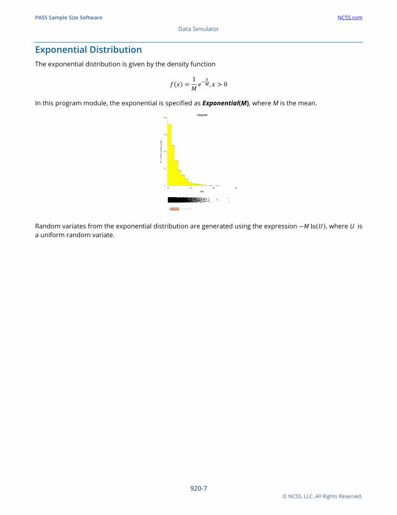
Exponential Distribution The exponential distribution is given by the density function

𝑓𝑓(𝑥𝑥) =1𝑀𝑀𝑀𝑀−

𝑥𝑥𝑀𝑀, 𝑥𝑥 > 0

In this program module, the exponential is specified as Exponential(M), where M is the mean.

Random variates from the exponential distribution are generated using the expression −𝑀𝑀 ln(𝑈𝑈), where U is a uniform random variate.




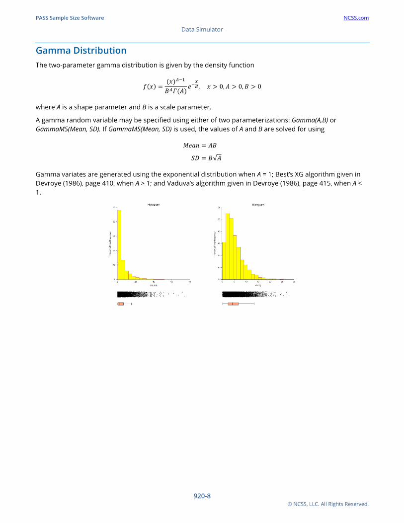
Gamma Distribution The two-parameter gamma distribution is given by the density function

𝑓𝑓(𝑥𝑥) =(𝑥𝑥)𝐴𝐴−1

𝐵𝐵𝐴𝐴𝛤𝛤(𝐴𝐴)𝑀𝑀−

𝑥𝑥𝐵𝐵, 𝑥𝑥 > 0,𝐴𝐴 > 0,𝐵𝐵 > 0

where A is a shape parameter and B is a scale parameter.

A gamma random variable may be specified using either of two parameterizations: Gamma(A,B) or GammaMS(Mean, SD). If GammaMS(Mean, SD) is used, the values of A and B are solved for using

𝑀𝑀𝑀𝑀𝑀𝑀𝑀𝑀 = 𝐴𝐴𝐵𝐵

𝑆𝑆𝐷𝐷 = 𝐵𝐵√𝐴𝐴

Gamma variates are generated using the exponential distribution when A = 1; Best’s XG algorithm given in Devroye (1986), page 410, when A > 1; and Vaduva’s algorithm given in Devroye (1986), page 415, when A < 1.




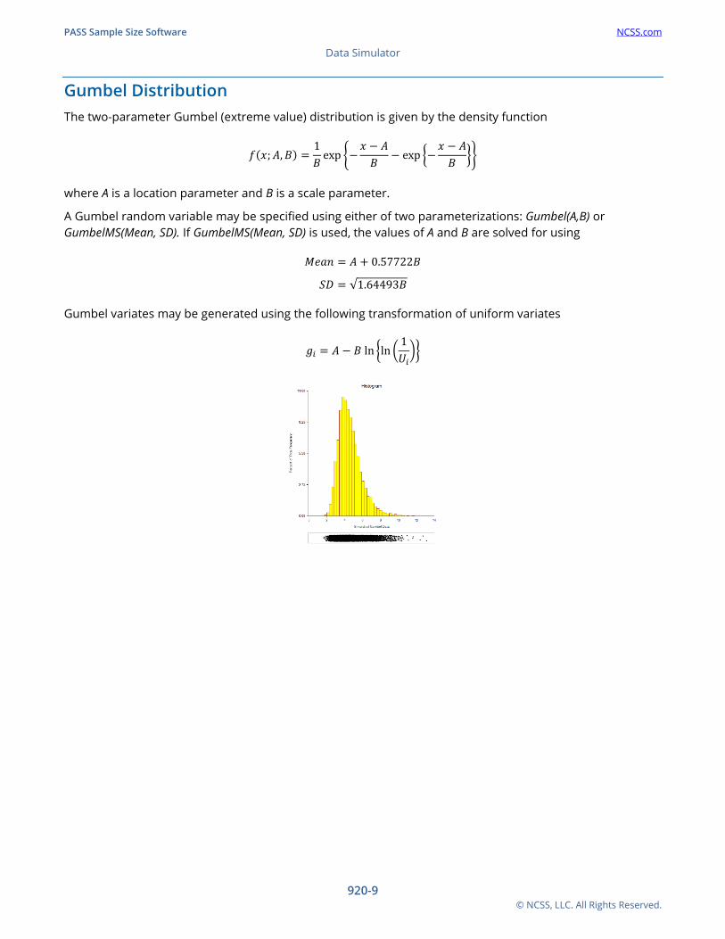
Gumbel Distribution The two-parameter Gumbel (extreme value) distribution is given by the density function

𝑓𝑓(𝑥𝑥;𝐴𝐴,𝐵𝐵) =1𝐵𝐵

exp �−𝑥𝑥 − 𝐴𝐴𝐵𝐵

− exp �−𝑥𝑥 − 𝐴𝐴𝐵𝐵

��

where A is a location parameter and B is a scale parameter.

A Gumbel random variable may be specified using either of two parameterizations: Gumbel(A,B) or GumbelMS(Mean, SD). If GumbelMS(Mean, SD) is used, the values of A and B are solved for using

𝑀𝑀𝑀𝑀𝑀𝑀𝑀𝑀 = 𝐴𝐴 + 0.57722𝐵𝐵

𝑆𝑆𝐷𝐷 = √1.64493𝐵𝐵

Gumbel variates may be generated using the following transformation of uniform variates

𝑔𝑔𝑖𝑖 = 𝐴𝐴 − 𝐵𝐵 ln �ln �1𝑈𝑈𝑖𝑖��




Laplace Distribution The two-parameter Laplace (or double-exponential) distribution is given by the density function

𝑓𝑓(𝑥𝑥;𝐴𝐴,𝐵𝐵) =1

2𝐵𝐵exp �−

|𝑥𝑥 − 𝐴𝐴|𝐵𝐵

�


A Laplace random variable may be specified using either of two parameterizations: Laplace(A, B) or LaplaceMS(Mean, SD). If LaplaceMS (Mean, SD) is used, the values of A and B are solved for using

𝑀𝑀𝑀𝑀𝑀𝑀𝑀𝑀 = 𝐴𝐴

𝑆𝑆𝐷𝐷 = 𝐵𝐵√2

Laplace variates are generated using the following transformation of uniform �− 12

< 𝑈𝑈 < 12� variates

𝑥𝑥𝑖𝑖 = 𝐴𝐴 − 𝐵𝐵 sgn(𝑈𝑈𝑖𝑖) ln(1 − 2|𝑈𝑈𝑖𝑖|)

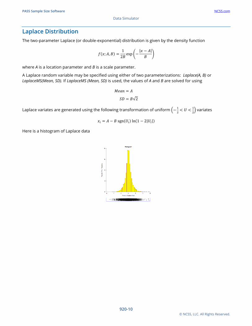
Here is a histogram of Laplace data




Logistic Distribution The two-parameter logistic distribution is given by the density function

𝑓𝑓(𝑥𝑥;𝐴𝐴,𝐵𝐵) =exp �−𝑥𝑥 − 𝐴𝐴

𝐵𝐵 �

𝐵𝐵 �1 + exp �−𝑥𝑥 − 𝐴𝐴𝐵𝐵 ��

2


A logistic random variable may be specified using either of two parameterizations: Logistic(A,B) or LogisticMS(Mean, SD). If LogisticMS(Mean, SD) is used, the values of A and B are solved for using

𝑀𝑀𝑀𝑀𝑀𝑀𝑀𝑀 = 𝐴𝐴

𝑆𝑆𝐷𝐷 =𝐵𝐵𝑆𝑆√3

Logistic variates are generated using the following transformation of uniform variates

𝑥𝑥𝑖𝑖 = 𝐴𝐴 + 𝐵𝐵 ln �𝑈𝑈𝑖𝑖

1 − 𝑈𝑈𝑖𝑖�

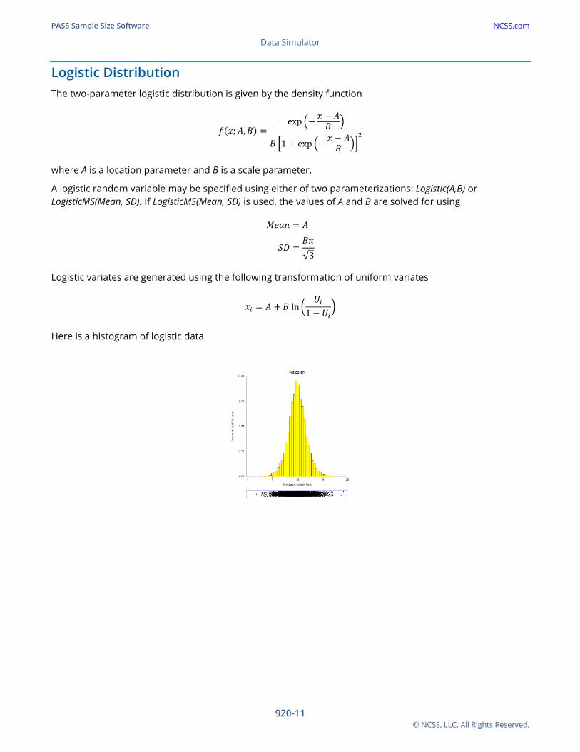
Here is a histogram of logistic data




Lognormal Distribution The two-parameter lognormal distribution is given by the density function

𝑓𝑓(𝑥𝑥;𝐴𝐴,𝐵𝐵) =1

𝑥𝑥𝐵𝐵√2𝑆𝑆exp �−

12�

ln(𝑥𝑥) − 𝐴𝐴𝐵𝐵

�2

�


A lognormal random variable may be specified using either of two parameterizations: Lognormal(A,B) or LognormalMS(Mean, SD). If LognormalMS (Mean, SD) is used, the values of A and B are solved for using

𝑀𝑀𝑀𝑀𝑀𝑀𝑀𝑀 = exp �𝐴𝐴 +𝐵𝐵2

2�

𝑆𝑆𝐷𝐷 = exp{2𝐴𝐴 + 𝐵𝐵2}[exp{𝐵𝐵2} − 1]

Lognormal variates are generated the following transformation of normal variates

𝑥𝑥𝑖𝑖 = exp(𝐴𝐴 + 𝐵𝐵 𝑧𝑧𝑖𝑖)

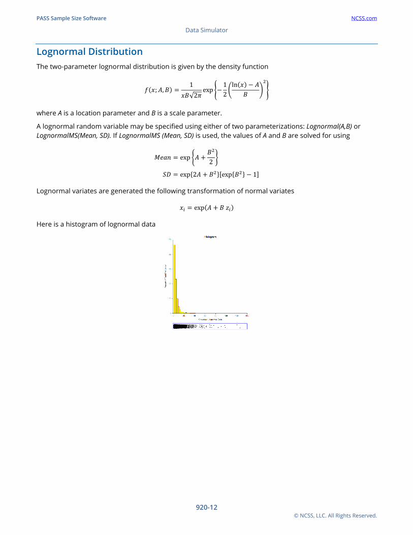
Here is a histogram of lognormal data




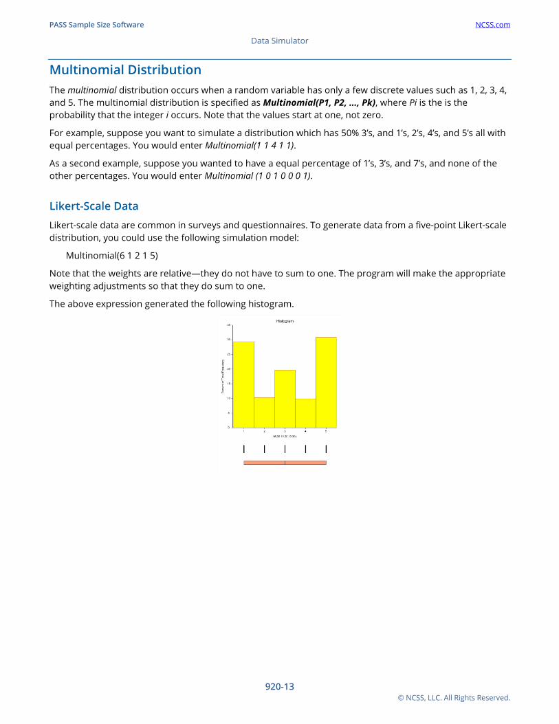
Multinomial Distribution The multinomial distribution occurs when a random variable has only a few discrete values such as 1, 2, 3, 4, and 5. The multinomial distribution is specified as Multinomial(P1, P2, …, Pk), where Pi is the is the probability that the integer i occurs. Note that the values start at one, not zero.

For example, suppose you want to simulate a distribution which has 50% 3’s, and 1’s, 2’s, 4’s, and 5’s all with equal percentages. You would enter Multinomial(1 1 4 1 1).

As a second example, suppose you wanted to have a equal percentage of 1’s, 3’s, and 7’s, and none of the other percentages. You would enter Multinomial (1 0 1 0 0 0 1).

Likert-Scale Data

Likert-scale data are common in surveys and questionnaires. To generate data from a five-point Likert-scale distribution, you could use the following simulation model:

Multinomial(6 1 2 1 5)

Note that the weights are relative—they do not have to sum to one. The program will make the appropriate weighting adjustments so that they do sum to one.

The above expression generated the following histogram.




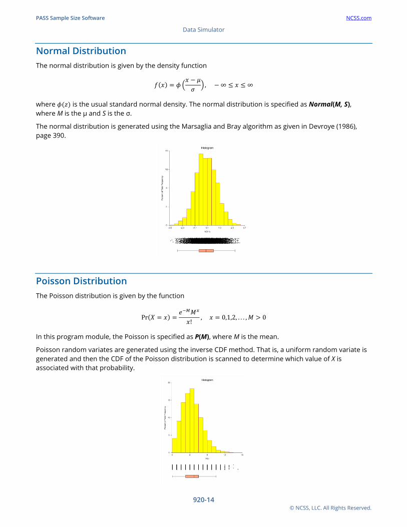
Normal Distribution The normal distribution is given by the density function

𝑓𝑓(𝑥𝑥) = 𝜙𝜙 �𝑥𝑥 − 𝜇𝜇𝜎𝜎

� , −∞ ≤ 𝑥𝑥 ≤ ∞

where 𝜙𝜙(𝑧𝑧) is the usual standard normal density. The normal distribution is specified as Normal(M, S), where M is the μ and S is the σ.

The normal distribution is generated using the Marsaglia and Bray algorithm as given in Devroye (1986), page 390.

Poisson Distribution The Poisson distribution is given by the function

Pr(𝑋𝑋 = 𝑥𝑥) =𝑀𝑀−𝑀𝑀𝑀𝑀𝑥𝑥

𝑥𝑥!, 𝑥𝑥 = 0,1,2, . . . ,𝑀𝑀 > 0

In this program module, the Poisson is specified as P(M), where M is the mean.

Poisson random variates are generated using the inverse CDF method. That is, a uniform random variate is generated and then the CDF of the Poisson distribution is scanned to determine which value of X is associated with that probability.




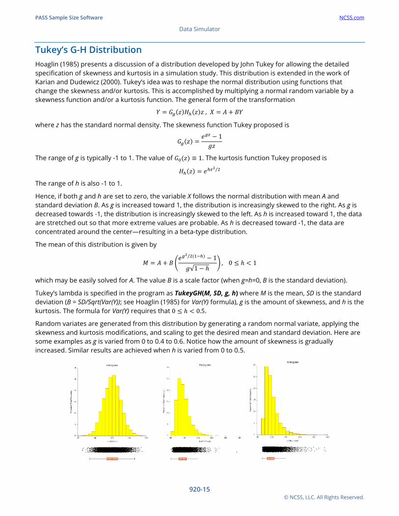
Tukey’s G-H Distribution Hoaglin (1985) presents a discussion of a distribution developed by John Tukey for allowing the detailed specification of skewness and kurtosis in a simulation study. This distribution is extended in the work of Karian and Dudewicz (2000). Tukey’s idea was to reshape the normal distribution using functions that change the skewness and/or kurtosis. This is accomplished by multiplying a normal random variable by a skewness function and/or a kurtosis function. The general form of the transformation

𝑌𝑌 = 𝐺𝐺𝑔𝑔(𝑧𝑧)𝐻𝐻ℎ(𝑧𝑧)𝑧𝑧 , 𝑋𝑋 = 𝐴𝐴 + 𝐵𝐵𝑌𝑌

where z has the standard normal density. The skewness function Tukey proposed is

𝐺𝐺𝑔𝑔(𝑧𝑧) =𝑀𝑀𝑔𝑔𝑔𝑔 − 1𝑔𝑔𝑧𝑧

The range of g is typically -1 to 1. The value of 𝐺𝐺0(𝑧𝑧) ≡ 1. The kurtosis function Tukey proposed is

𝐻𝐻ℎ(𝑧𝑧) = 𝑀𝑀ℎ𝑔𝑔2/2

The range of h is also -1 to 1.

Hence, if both g and h are set to zero, the variable X follows the normal distribution with mean A and standard deviation B. As g is increased toward 1, the distribution is increasingly skewed to the right. As g is decreased towards -1, the distribution is increasingly skewed to the left. As h is increased toward 1, the data are stretched out so that more extreme values are probable. As h is decreased toward -1, the data are concentrated around the center—resulting in a beta-type distribution.

The mean of this distribution is given by

𝑀𝑀 = 𝐴𝐴 + 𝐵𝐵 �𝑀𝑀𝑔𝑔2/2(1−ℎ) − 1𝑔𝑔√1 − ℎ

� , 0 ≤ ℎ < 1

which may be easily solved for A. The value B is a scale factor (when g=h=0, B is the standard deviation).

Tukey’s lambda is specified in the program as TukeyGH(M, SD, g, h) where M is the mean, SD is the standard deviation (B = SD/Sqrt(Var(Y)); see Hoaglin (1985) for Var(Y) formula), g is the amount of skewness, and h is the kurtosis. The formula for Var(Y) requires that 0 ≤ ℎ < 0.5.

Random variates are generated from this distribution by generating a random normal variate, applying the skewness and kurtosis modifications, and scaling to get the desired mean and standard deviation. Here are some examples as g is varied from 0 to 0.4 to 0.6. Notice how the amount of skewness is gradually increased. Similar results are achieved when h is varied from 0 to 0.5.




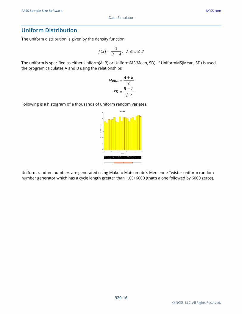
Uniform Distribution The uniform distribution is given by the density function

𝑓𝑓(𝑥𝑥) =1

𝐵𝐵 − 𝐴𝐴, 𝐴𝐴 ≤ 𝑥𝑥 ≤ 𝐵𝐵

The uniform is specified as either Uniform(A, B) or UniformMS(Mean, SD). If UniformMS(Mean, SD) is used, the program calculates A and B using the relationships

𝑀𝑀𝑀𝑀𝑀𝑀𝑀𝑀 =𝐴𝐴 + 𝐵𝐵

2

𝑆𝑆𝐷𝐷 =𝐵𝐵 − 𝐴𝐴√12

Following is a histogram of a thousands of uniform random variates.

Uniform random numbers are generated using Makoto Matsumoto’s Mersenne Twister uniform random number generator which has a cycle length greater than 1.0E+6000 (that’s a one followed by 6000 zeros).




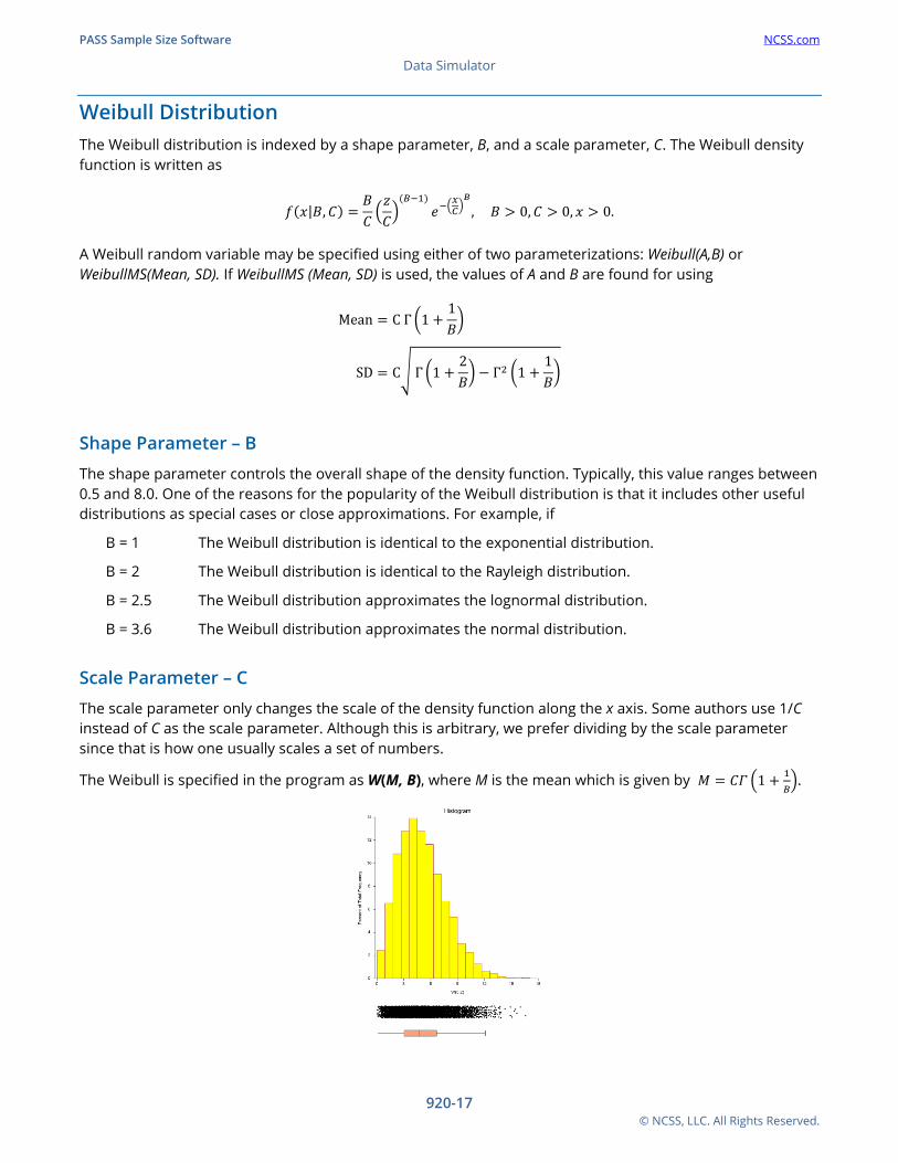
Weibull Distribution The Weibull distribution is indexed by a shape parameter, B, and a scale parameter, C. The Weibull density function is written as

𝑓𝑓(𝑥𝑥|𝐵𝐵,𝐶𝐶) =𝐵𝐵𝐶𝐶�𝑧𝑧𝐶𝐶�

(𝐵𝐵−1)𝑀𝑀−�

𝑥𝑥𝐶𝐶�

𝐵𝐵

, 𝐵𝐵 > 0,𝐶𝐶 > 0, 𝑥𝑥 > 0.

A Weibull random variable may be specified using either of two parameterizations: Weibull(A,B) or WeibullMS(Mean, SD). If WeibullMS (Mean, SD) is used, the values of A and B are found for using

Mean = C Γ �1 +1𝐵𝐵�

SD = C� Γ �1 +2𝐵𝐵� − Γ2 �1 +

1𝐵𝐵�

Shape Parameter – B

The shape parameter controls the overall shape of the density function. Typically, this value ranges between 0.5 and 8.0. One of the reasons for the popularity of the Weibull distribution is that it includes other useful distributions as special cases or close approximations. For example, if

B = 1 The Weibull distribution is identical to the exponential distribution.

B = 2 The Weibull distribution is identical to the Rayleigh distribution.

B = 2.5 The Weibull distribution approximates the lognormal distribution.

B = 3.6 The Weibull distribution approximates the normal distribution.

Scale Parameter – C

The scale parameter only changes the scale of the density function along the x axis. Some authors use 1/C instead of C as the scale parameter. Although this is arbitrary, we prefer dividing by the scale parameter since that is how one usually scales a set of numbers.

The Weibull is specified in the program as W(M, B), where M is the mean which is given by 𝑀𝑀 = 𝐶𝐶𝛤𝛤 �1 + 1𝐵𝐵�.




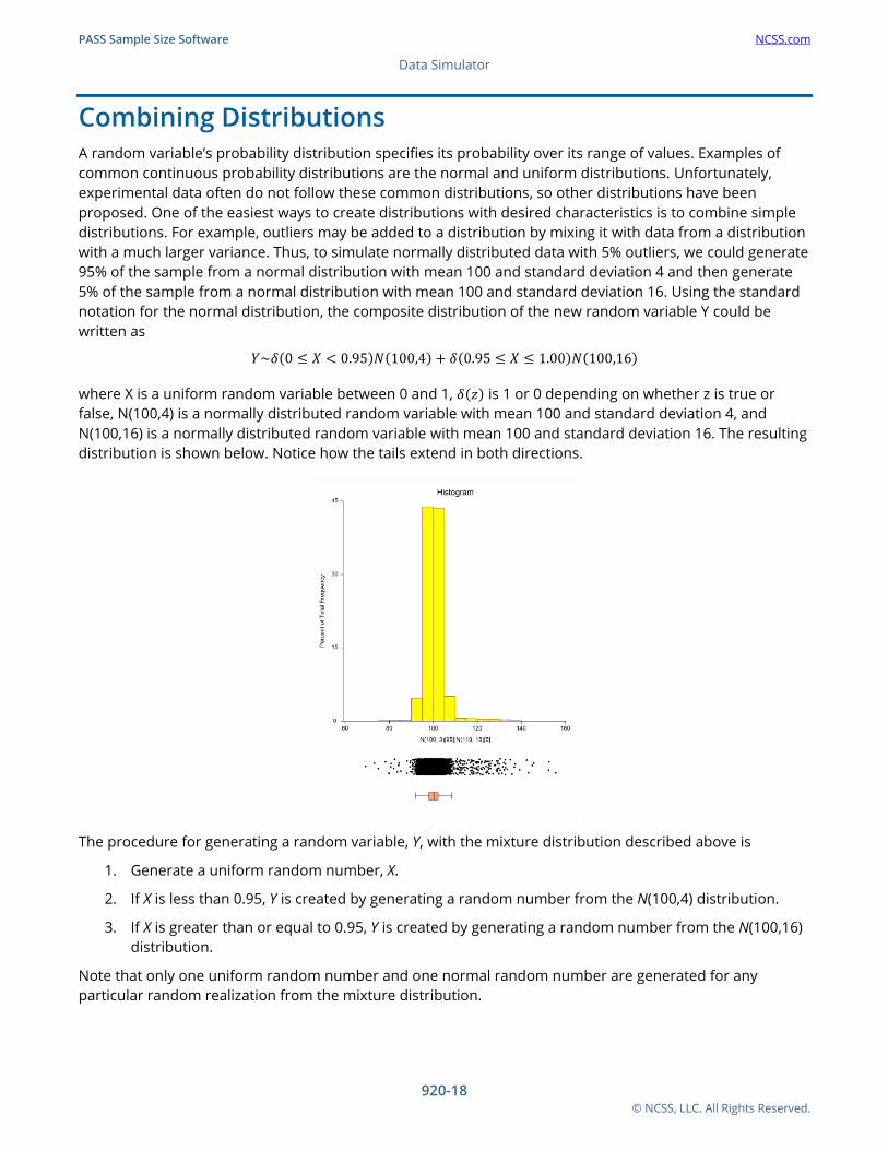
Combining Distributions A random variable’s probability distribution specifies its probability over its range of values. Examples of common continuous probability distributions are the normal and uniform distributions. Unfortunately, experimental data often do not follow these common distributions, so other distributions have been proposed. One of the easiest ways to create distributions with desired characteristics is to combine simple distributions. For example, outliers may be added to a distribution by mixing it with data from a distribution with a much larger variance. Thus, to simulate normally distributed data with 5% outliers, we could generate 95% of the sample from a normal distribution with mean 100 and standard deviation 4 and then generate 5% of the sample from a normal distribution with mean 100 and standard deviation 16. Using the standard notation for the normal distribution, the composite distribution of the new random variable Y could be written as

𝑌𝑌~𝛿𝛿(0 ≤ 𝑋𝑋 < 0.95)𝑁𝑁(100,4) + 𝛿𝛿(0.95 ≤ 𝑋𝑋 ≤ 1.00)𝑁𝑁(100,16)

where X is a uniform random variable between 0 and 1, 𝛿𝛿(𝑧𝑧) is 1 or 0 depending on whether z is true or false, N(100,4) is a normally distributed random variable with mean 100 and standard deviation 4, and N(100,16) is a normally distributed random variable with mean 100 and standard deviation 16. The resulting distribution is shown below. Notice how the tails extend in both directions.

The procedure for generating a random variable, Y, with the mixture distribution described above is

1. Generate a uniform random number, X.

2. If X is less than 0.95, Y is created by generating a random number from the N(100,4) distribution.

3. If X is greater than or equal to 0.95, Y is created by generating a random number from the N(100,16) distribution.

Note that only one uniform random number and one normal random number are generated for any particular random realization from the mixture distribution.




In general, the formula for a mixture random variable, Y, which is to be generated from two or more random variables defined by their distribution function 𝐹𝐹𝑖𝑖(𝑍𝑍𝑖𝑖) is given by

𝑌𝑌~�𝛿𝛿(𝑀𝑀𝑖𝑖 ≤ 𝑋𝑋 < 𝑀𝑀𝑖𝑖+1)𝐹𝐹𝑖𝑖(𝑍𝑍𝑖𝑖), 𝑀𝑀1 = 0 < 𝑀𝑀2 < ⋯ < 𝑀𝑀𝐾𝐾+1 = 1𝑘𝑘

𝑖𝑖=1

Note that the 𝑀𝑀𝑖𝑖 ’s are chosen so that weighting requirements are met. Also note that only one uniform random number and one other random number actually need to be generated for a particular value. The 𝐹𝐹𝑖𝑖(𝑍𝑍𝑖𝑖)’s may be any of the distributions which are listed below.

Since the test statistics which will be simulated are used to test hypotheses about one or more means, it will be convenient to parameterize the distributions in terms of their means.

Creating New Distributions using Expressions The set of probability distributions discussed above provides a basic set of useful distributions. However, you may want to mimic reality more closely by combining these basic distributions. For example, paired data is often analyzed by forming the differences of the two original variables. If the original data are normally distributed, then the differences are also normally distributed. Suppose, however, that the original data are exponential. The difference of two exponentials is not a common distribution.

Expression Syntax

The basic syntax is

C1 D1 operator1 C2 D2 operator2 C3 D3 operator3 …

where C1, C2, C3, etc. are coefficients (numbers), D1, D2, D3, etc. are probability distributions, and operator is one of the four symbols: +, -, *, /. Parentheses are only permitted in the specification of distributions.

Examples of valid expressions include

N(4, 5) – N(4, 5)

2E(3) – 4E(4) + 2E(5)

N(4, 2)/E(4)-K(5)

Notes about the Coefficients: C1, C2, C3

The coefficients may be positive or negative decimal numbers such as 2.3, 5, or -3.2. If no coefficient is specified, the coefficient is assumed to be one.

Notes about the Distributions: D1, D2, D3

The distributions may be any of the distributions listed above such as normal, exponential, or beta. The expressions are evaluated by generating random values from each of the distributions specified and then combining them according to the operators.

Notes about the operators: +, -, *, /

All multiplications and divisions are performed first, followed by any additions and subtractions.




Note that if only addition and subtraction are used in the expression, the mean of the resulting distribution is found by applying the same operations to the individual distribution means. If the expression involves multiplication or division, the mean of the resulting distribution is usually difficult to calculate directly.

Creating New Distributions using Mixtures Mixture distributions are formed by sampling a fixed percentage of the data from each of several distributions. For example, you may model outliers by obtaining 95% of your data from a normal distribution with a standard deviation of 5 and 5% of your data from a distribution with a standard deviation of 50.

Mixture Syntax

The basic syntax of a mixture is

D1[W1]; D2[W2]; …; Dk[Wk]

where the D’s represent distributions and the W’s represent weights. Note that the weights must be positive numbers. Also note that semi-colons are used to separate the components of the mixture.

Examples of valid mixture distributions include

N(4, 5)[19]; N(4, 50)[1] 95% of the distribution is N(4, 5), and the other 5% is N(4, 50).

W(4, 3)[7]; K(0)[3] 70% of the distribution is W(4, 3), and the other 30% is made up of zeros.

N(4, 2)-N(4,3)[2]; E(4)*E(2)[8] 20% of the distribution is N(4, 2)-N(4,3), and the other 80% is E(4)*E(2).

Notes about the Distributions

The distributions D1, D2, D3, etc. may be any valid distributional expression.

Notes about the Weights

The weights w1, w2, w3, etc. need not sum to one (or to one hundred). The program uses these weights to calculate new, internal weights that do sum to one. For example, if you enter weights of 1, 2, and 1, the internal weights will be 0.25, 0.50, and 0.25.

When a weight is not specified, it is assumed to have the value of ‘1.’ Thus

N(4, 5)[19]; N(4,50)[1]

is equivalent to

N(4, 5)[19]; N(4,50)




Special Functions A set of special functions is available to modify the generator number after all other operations are completed. These special functions are applied in the order they are given next.

Square Root (Absolute Value)

This function is activated by placing a ^ in the expression. When active, the square root of the absolute value of the number is used.

Logarithm (Absolute Value)

This function is activated by placing a ~ in the expression. When active, the logarithm (base e) of the absolute value of the number is used.

Exponential

This function is activated by placing an & in the expression. When active, the number is exponentiated to the base e. If the current number x is greater than 70, exp(70) is used rather than exp(x).

Absolute Value

This function is activated by placing a | in the expression. When active, the absolute value of the number is used.

Integer

This function is activated by placing a # in the expression. When active, the number is rounded to the nearest integer.




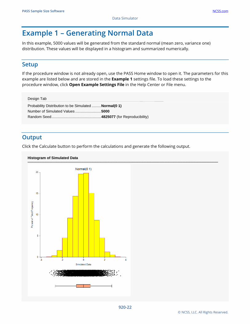
Example 1 – Generating Normal Data In this example, 5000 values will be generated from the standard normal (mean zero, variance one) distribution. These values will be displayed in a histogram and summarized numerically.

Setup If the procedure window is not already open, use the PASS Home window to open it. The parameters for this example are listed below and are stored in the Example 1 settings file. To load these settings to the procedure window, click Open Example Settings File in the Help Center or File menu.

Design Tab _____________ _______________________________________

Probability Distribution to be Simulated ......... Normal(0 1) Number of Simulated Values ......................... 5000 Random Seed ................................................ 4825077 (for Reproducibility)

Output Click the Calculate button to perform the calculations and generate the following output.

Histogram of Simulated Data ─────────────────────────────────────────────────────────────────────────




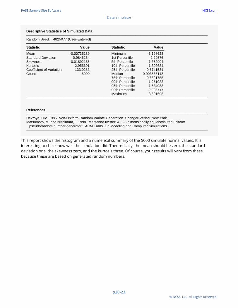
Descriptive Statistics of Simulated Data ───────────────────────────────────────────────────────────────────────── Random Seed: 4825077 (User-Entered) ───────────────────────────────────────────────────────────────────────── Statistic Value Statistic Value ────────────────────────────────────────────────────────────────────────────────────────────────────

Mean -0.00735189 Minimum -3.198628 Standard Deviation 0.9846264 1st Percentile -2.29576 Skewness 0.01892133 5th Percentile -1.632904 Kurtosis 2.955601 10th Percentile -1.302684 Coefficient of Variation -133.9283 25th Percentile -0.6741531 Count 5000 Median 0.003536118 75th Percentile 0.6621755 90th Percentile 1.251083 95th Percentile 1.634083 99th Percentile 2.293717 Maximum 3.501695 ───────────────────────────────────────────────────────────────────────── References ───────────────────────────────────────────────────────────────────────── Devroye, Luc. 1986. Non-Uniform Random Variate Generation. Springer-Verlag. New York. Matsumoto, M. and Nishimura,T. 1998. 'Mersenne twister: A 623-dimensionally equidistributed uniform pseudorandom number generator.' ACM Trans. On Modeling and Computer Simulations. ─────────────────────────────────────────────────────────────────────────

This report shows the histogram and a numerical summary of the 5000 simulate normal values. It is interesting to check how well the simulation did. Theoretically, the mean should be zero, the standard deviation one, the skewness zero, and the kurtosis three. Of course, your results will vary from these because these are based on generated random numbers.




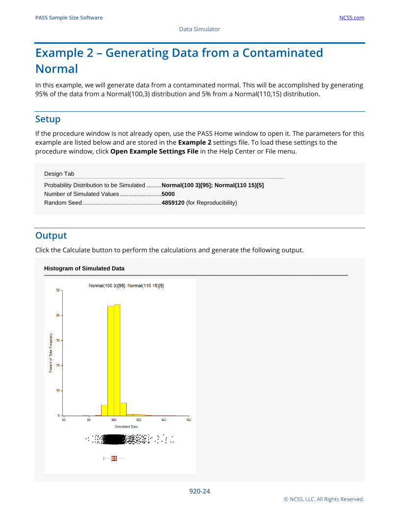
Example 2 – Generating Data from a Contaminated Normal In this example, we will generate data from a contaminated normal. This will be accomplished by generating 95% of the data from a Normal(100,3) distribution and 5% from a Normal(110,15) distribution.


Design Tab _____________ _______________________________________

Probability Distribution to be Simulated ......... Normal(100 3)[95]; Normal(110 15)[5] Number of Simulated Values ......................... 5000 Random Seed ................................................ 4859120 (for Reproducibility)






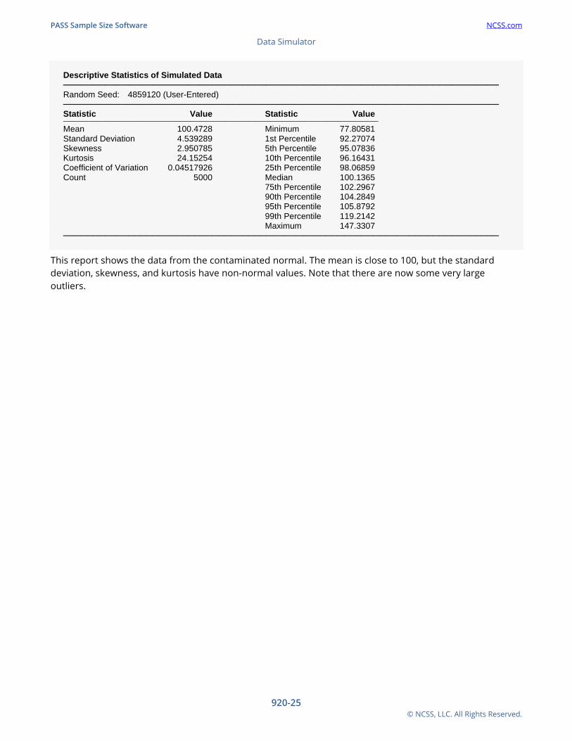
Descriptive Statistics of Simulated Data ───────────────────────────────────────────────────────────────────────── Random Seed: 4859120 (User-Entered) ───────────────────────────────────────────────────────────────────────── Statistic Value Statistic Value ───────────────────────────────────────────────────────────────────────────────────────────────

Mean 100.4728 Minimum 77.80581 Standard Deviation 4.539289 1st Percentile 92.27074 Skewness 2.950785 5th Percentile 95.07836 Kurtosis 24.15254 10th Percentile 96.16431 Coefficient of Variation 0.04517926 25th Percentile 98.06859 Count 5000 Median 100.1365 75th Percentile 102.2967 90th Percentile 104.2849 95th Percentile 105.8792 99th Percentile 119.2142 Maximum 147.3307 ─────────────────────────────────────────────────────────────────────────

This report shows the data from the contaminated normal. The mean is close to 100, but the standard deviation, skewness, and kurtosis have non-normal values. Note that there are now some very large outliers.




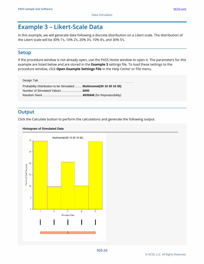
Example 3 – Likert-Scale Data In this example, we will generate data following a discrete distribution on a Likert scale. The distribution of the Likert scale will be 30% 1’s, 10% 2’s, 20% 3’s, 10% 4’s, and 30% 5’s.


Design Tab _____________ _______________________________________

Probability Distribution to be Simulated ......... Multinomial(30 10 20 10 30) Number of Simulated Values ......................... 5000 Random Seed ................................................ 4935948 (for Reproducibility)






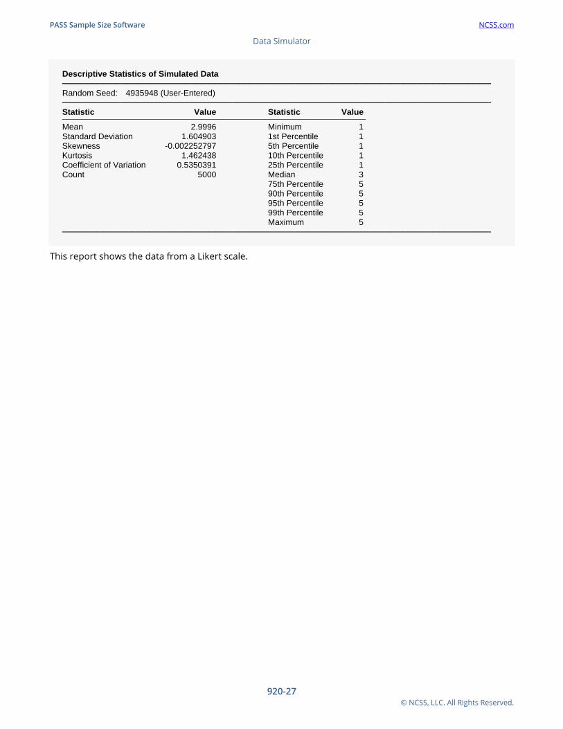
Descriptive Statistics of Simulated Data ───────────────────────────────────────────────────────────────────────── Random Seed: 4935948 (User-Entered) ───────────────────────────────────────────────────────────────────────── Statistic Value Statistic Value ─────────────────────────────────────────────────────────────────────────────────────────────

Mean 2.9996 Minimum 1 Standard Deviation 1.604903 1st Percentile 1 Skewness -0.002252797 5th Percentile 1 Kurtosis 1.462438 10th Percentile 1 Coefficient of Variation 0.5350391 25th Percentile 1 Count 5000 Median 3 75th Percentile 5 90th Percentile 5 95th Percentile 5 99th Percentile 5 Maximum 5 ─────────────────────────────────────────────────────────────────────────

This report shows the data from a Likert scale.




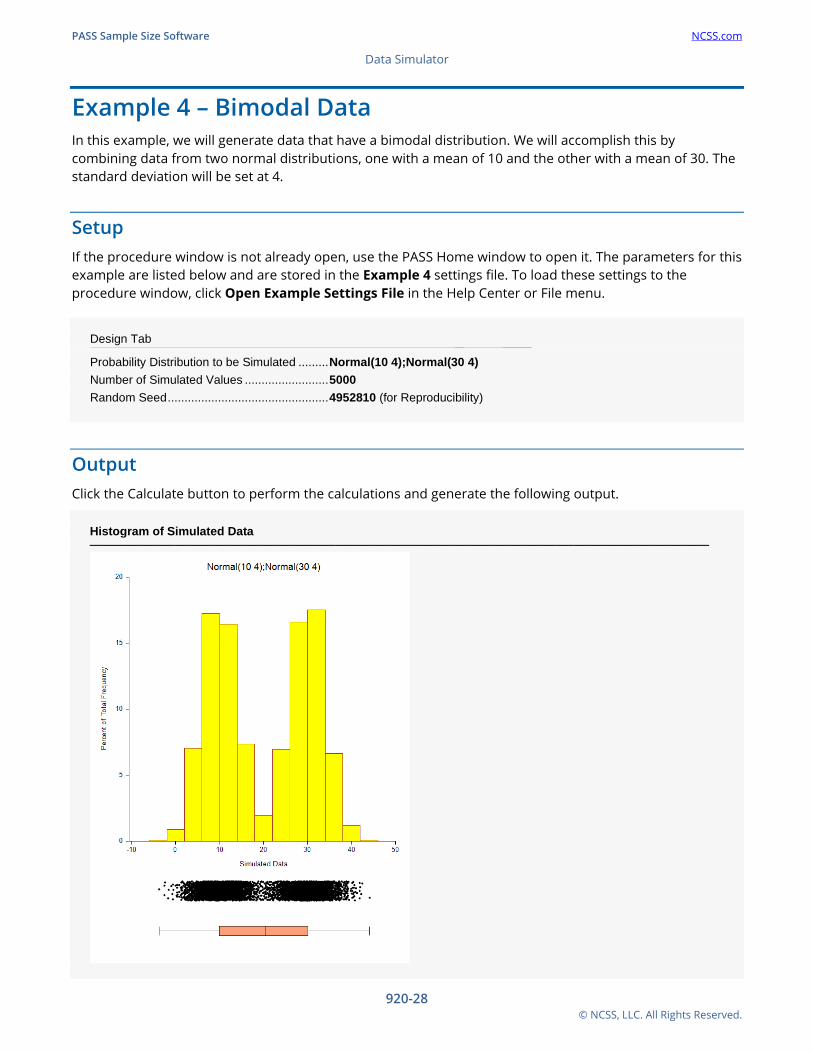
Example 4 – Bimodal Data In this example, we will generate data that have a bimodal distribution. We will accomplish this by combining data from two normal distributions, one with a mean of 10 and the other with a mean of 30. The standard deviation will be set at 4.


Design Tab _____________ _______________________________________

Probability Distribution to be Simulated ......... Normal(10 4);Normal(30 4) Number of Simulated Values ......................... 5000 Random Seed ................................................ 4952810 (for Reproducibility)






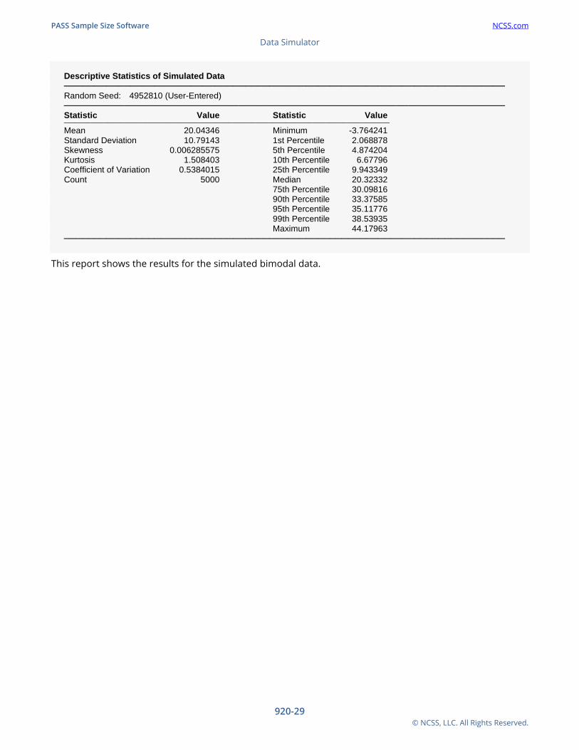
Descriptive Statistics of Simulated Data ───────────────────────────────────────────────────────────────────────── Random Seed: 4952810 (User-Entered) ───────────────────────────────────────────────────────────────────────── Statistic Value Statistic Value ─────────────────────────────────────────────────────────────────────────────────────────────────

Mean 20.04346 Minimum -3.764241 Standard Deviation 10.79143 1st Percentile 2.068878 Skewness 0.006285575 5th Percentile 4.874204 Kurtosis 1.508403 10th Percentile 6.67796 Coefficient of Variation 0.5384015 25th Percentile 9.943349 Count 5000 Median 20.32332 75th Percentile 30.09816 90th Percentile 33.37585 95th Percentile 35.11776 99th Percentile 38.53935 Maximum 44.17963 ─────────────────────────────────────────────────────────────────────────

This report shows the results for the simulated bimodal data.




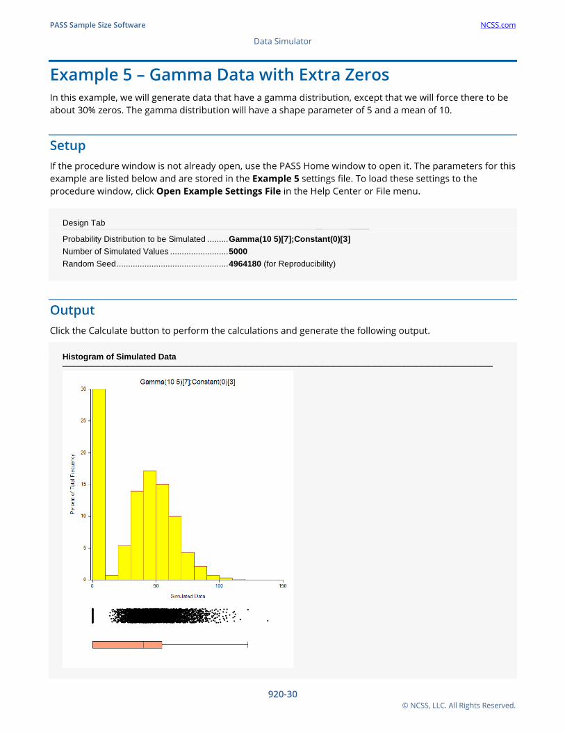
Example 5 – Gamma Data with Extra Zeros In this example, we will generate data that have a gamma distribution, except that we will force there to be about 30% zeros. The gamma distribution will have a shape parameter of 5 and a mean of 10.


Design Tab _____________ _______________________________________

Probability Distribution to be Simulated ......... Gamma(10 5)[7];Constant(0)[3] Number of Simulated Values ......................... 5000 Random Seed ................................................ 4964180 (for Reproducibility)






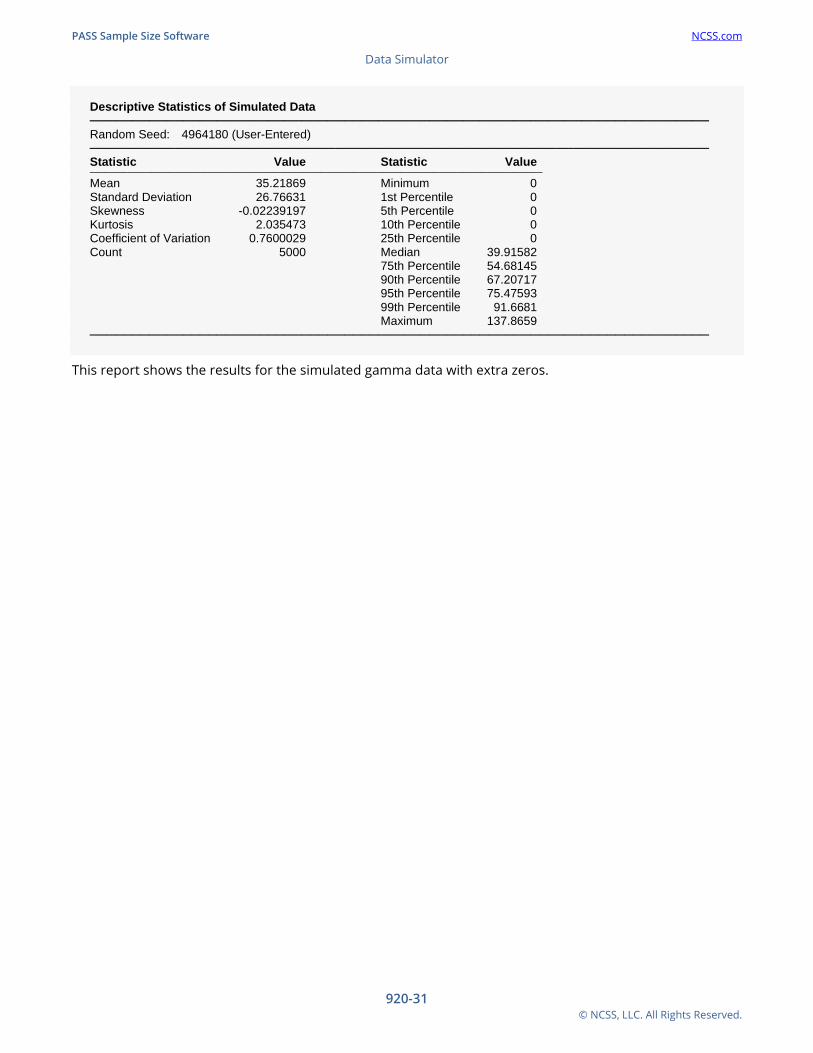
Descriptive Statistics of Simulated Data ───────────────────────────────────────────────────────────────────────── Random Seed: 4964180 (User-Entered) ───────────────────────────────────────────────────────────────────────── Statistic Value Statistic Value ────────────────────────────────────────────────────────────────────────────────────────────────

Mean 35.21869 Minimum 0 Standard Deviation 26.76631 1st Percentile 0 Skewness -0.02239197 5th Percentile 0 Kurtosis 2.035473 10th Percentile 0 Coefficient of Variation 0.7600029 25th Percentile 0 Count 5000 Median 39.91582 75th Percentile 54.68145 90th Percentile 67.20717 95th Percentile 75.47593 99th Percentile 91.6681 Maximum 137.8659 ─────────────────────────────────────────────────────────────────────────

This report shows the results for the simulated gamma data with extra zeros.




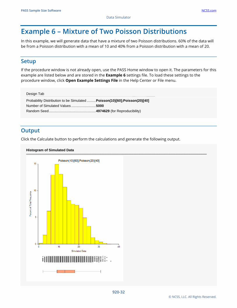
Example 6 – Mixture of Two Poisson Distributions In this example, we will generate data that have a mixture of two Poisson distributions. 60% of the data will be from a Poisson distribution with a mean of 10 and 40% from a Poisson distribution with a mean of 20.


Design Tab _____________ _______________________________________

Probability Distribution to be Simulated ......... Poisson(10)[60];Poisson(20)[40] Number of Simulated Values ......................... 5000 Random Seed ................................................ 4974629 (for Reproducibility)






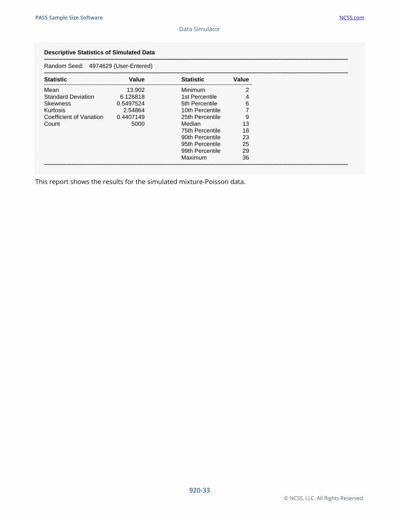
Descriptive Statistics of Simulated Data ───────────────────────────────────────────────────────────────────────── Random Seed: 4974629 (User-Entered) ───────────────────────────────────────────────────────────────────────── Statistic Value Statistic Value ──────────────────────────────────────────────────────────────────────────────────────────

Mean 13.902 Minimum 2 Standard Deviation 6.126818 1st Percentile 4 Skewness 0.5497524 5th Percentile 6 Kurtosis 2.54864 10th Percentile 7 Coefficient of Variation 0.4407149 25th Percentile 9 Count 5000 Median 13 75th Percentile 18 90th Percentile 23 95th Percentile 25 99th Percentile 29 Maximum 36 ─────────────────────────────────────────────────────────────────────────

This report shows the results for the simulated mixture-Poisson data.




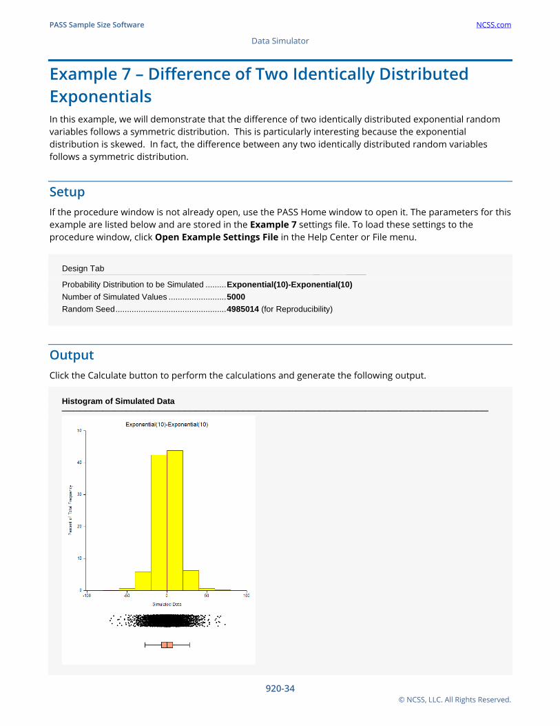
Example 7 – Difference of Two Identically Distributed Exponentials In this example, we will demonstrate that the difference of two identically distributed exponential random variables follows a symmetric distribution. This is particularly interesting because the exponential distribution is skewed. In fact, the difference between any two identically distributed random variables follows a symmetric distribution.


Design Tab _____________ _______________________________________

Probability Distribution to be Simulated ......... Exponential(10)-Exponential(10) Number of Simulated Values ......................... 5000 Random Seed ................................................ 4985014 (for Reproducibility)






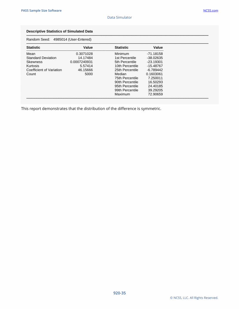
Descriptive Statistics of Simulated Data ───────────────────────────────────────────────────────────────────────── Random Seed: 4985014 (User-Entered) ───────────────────────────────────────────────────────────────────────── Statistic Value Statistic Value ───────────────────────────────────────────────────────────────────────────────────────────────────

Mean 0.3071028 Minimum -71.18158 Standard Deviation 14.17484 1st Percentile -38.02635 Skewness 0.0007240931 5th Percentile -23.19301 Kurtosis 5.57414 10th Percentile -15.48767 Coefficient of Variation 46.15666 25th Percentile -6.789442 Count 5000 Median 0.1603061 75th Percentile 7.250011 90th Percentile 16.50293 95th Percentile 24.40185 99th Percentile 39.29205 Maximum 72.90659 ─────────────────────────────────────────────────────────────────────────

This report demonstrates that the distribution of the difference is symmetric.


chapter 920 data simulator - ncss

Documents