chemtech - university of michiganessen/html/byconcept/cdchap/14chap/... · ... in complex systems...
TRANSCRIPT

© 2006 Pearson Education, Inc.All rights reserved.
From Elements of Chemical Reaction Engineering,Fourth Edition, by H. Scott Fogler.
945
DVD
14
Models for NonidealReactors
Success is a journey, not a destination.Ben Sweetland
Use the RTD toevaluate
parameters
Overview Not all tank reactors are perfectly mixed nor do all tubular reac-tors exhibit plug-flow behavior. In these situations, some means must beused to allow for deviations from ideal behavior. Chapter 13 showed howthe RTD was sufficient if the reaction was first order or if the fluid waseither in a state of complete segregation or maximum mixedness. We usethe segregation and maximum mixedness models to bound the conversionwhen no adjustable parameters are used. For non-first-order reactions in afluid with good micromixing, more than just the RTD is needed. These sit-uations compose a great majority of reactor analysis problems and cannotbe ignored. For example, we may have an existing reactor and want to carryout a new reaction in that reactor. To predict conversions and product distri-butions for such systems, a model of reactor flow patterns is necessary. Tomodel these patterns, we use combinations and/or modifications of idealreactors to represent real reactors. With this technique, we classify a modelas being either a one-parameter model (e.g., tanks-in-series model or disper-sion model) or a two-parameter model (e.g., reactor with bypassing anddead volume). The RTD is then used to evaluate the parameter(s) in themodel. After completing this chapter, the reader will be able to apply thetanks-in-series model and the dispersion model to tubular reactors. In addi-tion, the reader will be able to suggest combinations of ideal reactors tomodel a real reactor.

© 2006 Pearson Education, Inc.All rights reserved.
From Elements of Chemical Reaction Engineering,Fourth Edition, by H. Scott Fogler.
946
Models for Nonideal Reactors Chap. 14
14.1 Some Guidelines
The overall goal is to use the following equation
The choice of the particular model to be used depends largely on the engineer-ing judgment of the person carrying out the analysis. It is this person’s job tochoose the model that best combines the conflicting goals of mathematicalsimplicity and physical realism. There is a certain amount of art in the devel-opment of a model for a particular reactor, and the examples presented herecan only point toward a direction that an engineer’s thinking might follow.
For a given real reactor, it is not uncommon to use all the models dis-cussed previously to predict conversion and then make a comparison. Usually,the real conversion will be
bounded
by the model calculations.The following guidelines are suggested when developing models for non-
ideal reactors:
1.
The model must be mathematically tractable
. The equations used todescribe a chemical reactor should be able to be solved without aninordinate expenditure of human or computer time.
2.
The model must realistically describe the characteristics of the non-ideal reactor
. The phenomena occurring in the nonideal reactor mustbe reasonably described physically, chemically, and mathematically.
3.
The model must not have more than two adjustable parameters
. Thisconstraint is used because an expression with more than two adjust-able parameters can be fitted to a great variety of experimental data,and the modeling process in this circumstance is nothing more thanan exercise in curve fitting. The statement “Give me four adjustableparameters and I can fit an elephant; give me five and I can includehis tail!” is one that I have heard from many colleagues. Unless oneis into modern art, a substantially larger number of adjustable param-eters is necessary to draw a reasonable-looking elephant.
1
Aone-parameter model is, of course, superior to a two-parameter modelif the one-parameter model is sufficiently realistic. To be fair, how-ever, in complex systems (e.g., internal diffusion and conduction,mass transfer limitations) where other parameters may be measured
independently
, then more than two parameters are quite acceptable.
Table 14-1 gives some guidelines that will help your analysis and model build-ing of nonideal reaction systems.
1
J. Wei,
CHEMTECH
,
5
, 128 (1975).
RTD Data + Kinetics + Model = Prediction
Conflicting goals
A Model Must• Fit the data• Be able to
extrapolate theory and experiment
• Have realistic parameters

© 2006 Pearson Education, Inc.All rights reserved.
From Elements of Chemical Reaction Engineering,Fourth Edition, by H. Scott Fogler.
Sec. 14.1 Some Guidelines
947
14.1.1 One-Parameter Models
Here we use a single parameter to account for the nonideality of our reactor.This parameter is most always evaluated by analyzing the RTD determinedfrom a tracer test. Examples of one-parameter models for nonideal CSTRsinclude a reactor dead volume
V
D
, where no reaction takes place, or a fraction
f
of fluid bypassing the reactor, thereby exiting unreacted. Examples ofone-parameter models for tubular reactors include the tanks-in-series modeland the dispersion model. For the tanks-in-series model, the parameter is thenumber of tanks,
n
, and for the dispersion model, it is the dispersion coeffi-cient,
D
a
. Knowing the parameter values, we then proceed to determine theconversion and/or effluent concentrations for the reactor.
We first consider nonideal tubular reactors. Tubular reactors may beempty, or they may be packed with some material that acts as a catalyst,heat-transfer medium, or means of promoting interphase contact. Until nowwhen analyzing ideal tubular reactors, it usually has been assumed that the fluidmoved through the reactor in piston-like flow (PFR), and every atom spends anidentical length of time in the reaction environment. Here, the
velocity profileis flat,
and there is no axial mixing. Both of these assumptions are false to someextent in every tubular reactor; frequently, they are sufficiently false to warrantsome modification. Most popular tubular reactor models need to have means toallow for failure of the plug-flow model and insignificant axial mixing assump-tions; examples include the unpacked laminar flow tubular reactor, theunpacked turbulent flow, and packed-bed reactors. One of two approaches isusually taken to compensate for failure of either or both of the ideal assump-tions. One approach involves modeling the nonideal tubular reactor as a series
T
ABLE
14-1.
A P
ROCEDURE
FOR
C
HOOSING
A
M
ODEL
TO
P
REDICT
THE
O
UTLET
C
ONCENTRATION
AND
C
ONVERSION
1.
Look at the reactor.
a. Where are the inlet and outlet streams to and from the reactors? (Isby-passing a possibility?)
b. Look at the mixing system. How many impellers are there? (Could there be multiple mixing zones in the reactor?)
c. Look at the configuration. (Is internal recirculation possible? Is the packing of the catalyst particles loose so channeling could occur?)
2.
Look at the tracer data.
a. Plot the E(t) and F(t) curves.b. Plot and analyze the shapes of the E(
Q
) and F(
Q
) curves. Is the shape of the curve such that the curve or parts of the curve can be fit by an ideal reactor model? Does the curve have a long tail suggesting a stagnant zone? Does the curve have an early spike indicating bypassing?
c. Calculate the mean residence time, t
m
, and variance,
s
2
. How does the t
m
determined from the RTD data compare with
t
as measured with a yardstick and flow meter? How large is the variance; is it larger or smaller than
t
2
?3.
Choose a model or perhaps two or three models.
4.
Use the tracer data to determine the model parameters
(e.g., n, D
a
,
v
b
).5.
Use the CRE algorithm in Chapter 4.
Calculate the exit concentrations and conver-sion for the model system you have selected.
The Guidelines
Nonideal tubularreactors

© 2006 Pearson Education, Inc.All rights reserved.
From Elements of Chemical Reaction Engineering,Fourth Edition, by H. Scott Fogler.
948
Models for Nonideal Reactors Chap. 14
of identically sized CSTRs. The other approach (the dispersion model) involvesa modification of the ideal reactor by imposing axial dispersion on plug flow.
14.1.2 Two-Parameter Models
The premise for the two-parameter model is that we can use a combination ofideal reactors to model the real reactor. For example, consider a packed bedreactor with channeling. Here the response to a pulse tracer input would showtwo dispersed pulses in the output as shown in Figure 13-10 and Figure 14-1.
Here we could model the real reactor as two ideal PBRs in parallel with thetwo parameters being the fluid that channels,
v
b
, and the reactor dead volume,
V
D
. The real reactor voume is
V
=
V
D
+
V
S
with
v
0
=
v
b
+
v
S
.
14.2 Tanks-in-Series (T-I-S) Model
In this section we discuss the use of the tanks-in-series (T-I-S) model todescribe nonideal reactors and calculate conversion. The T-I-S model is aone-parameter model. We will analyze the RTD to determine the number ofideal tanks,
n
, in series that will give approximately the same RTD as the non-ideal reactor. Next we will apply the reaction engineering algorithm developedin Chapters 1 through 4 to calculate conversion. We are first going to developthe RTD equation for three tanks in series (Figure 14-2) and then generalize to
n
reactors in series to derive an equation that gives the number of tanks inseries that best fits the RTD data.
t
Channeling
C(t)VS
VD
(a) (b) (c)
Dead Zonesz = 0 z = L
vS
v
vv
Figure 14-1 (a) Real system; (b) outlet for a pulse input; (c) model system.
n = ?
In Figure 2-9, wesaw how tanks in
series could approxi-mate a PFR.
Pulse
Pulse
1
2
3
(b)(a)
Figure 14-2 Tanks in series: (a) real system, (b) model system.

© 2006 Pearson Education, Inc.All rights reserved.
From Elements of Chemical Reaction Engineering,Fourth Edition, by H. Scott Fogler.
Sec. 14.2 Tanks-in-Series (T-I-S) Model
949
The RTD will be analyzed from a tracer pulse injected into the first reac-tor of three equally sized CSTRs in series. Using the definition of the RTDpresented in Section 13.2, the fraction of material leaving the system of threereactors (i.e., leaving the third reactor) that has been in the system betweentime
t
and
t
�
�
t
is
E
(
t
)
�
t
�
Then
E
(
t
)
�
(14-1)
In this expression,
C
3
(
t
) is the concentration of tracer in the effluent from thethird reactor and the other terms are as defined previously.
It is now necessary to obtain the outlet concentration of tracer, C3(t), asa function of time. As in a single CSTR, a material balance on the first reactorgives
(14-2)
Integrating gives the expression for the tracer concentration in the effluentfrom the first reactor:
C1 � C0 � C0 (14-3)
The volumetric flow rate is constant and all the reactor volumes areidentical (V1 � V2 � Vi ); therefore, all the space times of the individual reac-tors are identical (t1 � t2 � ti ). Because Vi is the volume of a single reactorin the series, ti here is the residence time in one of the reactors, not in theentire reactor system (i.e., ti � t/n).
A material balance on the tracer in the second reactor gives
Using Equation (14-3) to substitute for C1, we obtain the first-order ordinarydifferential equation
vC3 t( ) �t
N0
-----------------------C3 t( )
C 3 t ( ) t d
0
� �
------------------------------ � t �
C3 t( )
C 3 t ( ) t d
0
� �
------------------------------
V1 dC
1 dt --------- v C 1 ��
We perform atracer balance on
each reactor toobtain C3(t)
e vt V1�� e t t1��
C0 N0 V1�
v0 C 3 t ( ) td 0
�
�
V
1
-----------------------------------� �
v v0�( )
V2 dC
2 dt --------- v C 1 v C 2 ��
© 2006 Pearson Education, Inc.All rights reserved.
From Elements of Chemical Reaction Engineering,Fourth Edition, by H. Scott Fogler.
950
Models for Nonideal Reactors Chap. 14
This equation is readily solved using an integrating factor along with theinitial condition
C
2
�
0 at
t
�
0, to give
(14-4)
The same procedure used for the third reactor gives the expression for the con-centration of tracer in the effluent from the third reactor (and therefore fromthe reactor system),
(14-5)
Substituting Equation (14-5) into Equation (14-1), we find that
E
(
t
)
�
�
(14-6)
Generalizing this method to a series of
n
CSTRs gives the RTD for
n
CSTRs in series,
E
(
t
):
(14-7)
Because the total reactor volume is
nV
i
, then
t
i
�
t
/
n
, where
t
represents thetotal reactor volume divided by the flow rate, :
E
(
�
)
�
t
E
(
t
) =
e
�
n
�
(14-8)
where
�
�
t
/
t
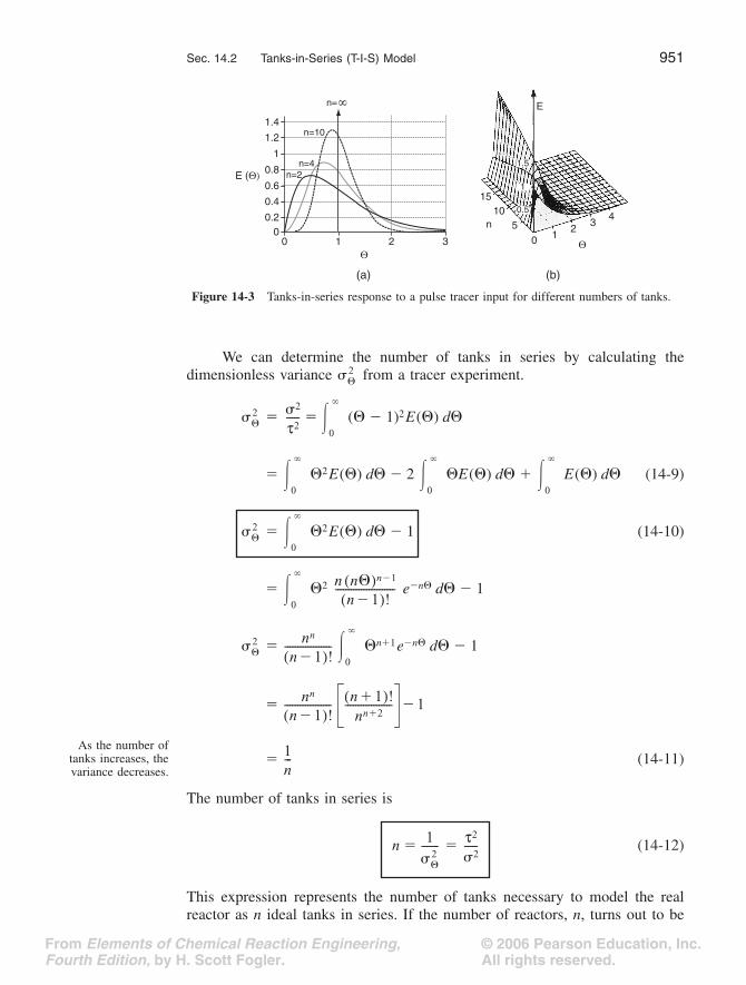
.Figure 14-3 illustrates the RTDs of various numbers of CSTRs in series
in a two-dimensional plot (a) and in a three-dimensional plot (b). As the num-ber becomes very large, the behavior of the system approaches that of aplug-flow reactor.
dC2
dt---------
C2
ti
------�C0
ti
------ e �
t
t
i
� �
et t i�
C2C0 t
ti
-------- e �
t
t
i
� �
C3C0 t2
2ti2
---------- e �
t
t
i
� �
C3 t( )
C3 t( ) td0
�
�-----------------------
C0t2/ 2ti2( )e
t/ti�
C0t2et/ti�
2ti2
---------------------dt0
�
�------------------------------------�
t2
2ti3
-------- e �
t
t
i
�
RTD for equal-sizetanks in series E t( ) t n�1
n 1�( )!tin
------------------------ e �
t
t
i � �
v
n n�( )n�1
n 1�( )!-----------------------
© 2006 Pearson Education, Inc.All rights reserved.
From Elements of Chemical Reaction Engineering,Fourth Edition, by H. Scott Fogler.
Sec. 14.2 Tanks-in-Series (T-I-S) Model
951
We can determine the number of tanks in series by calculating thedimensionless variance from a tracer experiment.
�
(
�
�
1)
2
E
(
�
)
d
�
� �
2
E
(
�
)
d
�
�
2
�
E
(
�
)
d
�
�
E
(
�
)
d
� (14-9)
� �2E(�) d� � 1 (14-10)
� �2 e�n� d� � 1
� �n�1e�n� d� � 1
�
� (14-11)
The number of tanks in series is
(14-12)
This expression represents the number of tanks necessary to model the realreactor as n ideal tanks in series. If the number of reactors, n, turns out to be
1.4n=10
n=∞
n=4n=2
1.2
1
0.8
0.6
0.4
0.20
0 1 2
(a) (b)
3
510
15
0
E
12
34
0.5
1
1.5
n
Figure 14-3 Tanks-in-series response to a pulse tracer input for different numbers of tanks.
�2
�2 2
t2-----
0
� �
�
0
� �
0
� �
0
� �
�2
0
� �
0
� � n n�( )n�1
n 1�
( )
!-----------------------
�2 nn
n 1�( )!------------------
0
� �
nn
n 1�( )!------------------ n 1
� ( ) !
n n
�
2 ------------------ 1 �
As the number oftanks increases, thevariance decreases.
1n---
n 1�
2------- t2
2-----� �

© 2006 Pearson Education, Inc.All rights reserved.
From Elements of Chemical Reaction Engineering,Fourth Edition, by H. Scott Fogler.
952
Models for Nonideal Reactors Chap. 14
small, the reactor characteristics turn out to be those of a single CSTR or per-haps two CSTRs in series. At the other extreme, when
n
turns out to be large,we recall from Chapter 2 the reactor characteristics approach those of a PFR.
If the reaction is first order, we can use Equation (4-11) to calculate theconversion,
X
�
1
�
(4-11)
where
t
i
�
It is acceptable (and usual) for the value of
n
calculated from Equation (14-12)to be a noninteger in Equation (4-11) to calculate the conversion. For reactionsother than first order, an integer number of reactors must be used and sequen-tial mole balances on each reactor must be carried out. If, for example,
n
=2.53, then one could calculate the conversion for two tanks and also for threetanks to bound the conversion. The conversion and effluent concentrationswould be solved sequentially using the algorithm developed in Chapter 4. Thatis, after solving for the effluent from the first tank, it would be used as theinput to the second tank and so on as shown in Table 14-2.
T
ABLE
14-2.
T
ANKS
-I
N
-S
ERIES
S
ECOND
-O
RDER
R
EACTION
Two-Reactor System Three-Reactor System
For two equally sized reactors For three equally sized reactors
For a second-order reaction, the combined mole balance, rate law, and stoichiometry for the first reactor gives
Solving for C
Aout
Two-Reactor System: Three-Reactor System:
Solving for exit concentration from reactor 1 for each reactor system gives
The exit concentration from the second reactor for each reactor system gives
11 ti k�( )n
-----------------------
Vv0 n---------
V V1 V2��
V1 V2V2---� �
t2V2
v0
----- V/2v0
-------- t2---� � �
V V1 V2 V3� ��
V1 V2 V3 V/3� � �
t1 t2 t3V/3v0
-------- t3---� � � �
t CAin CAout�
k1CAout2
----------------------------�
CAout1� 1 4ktCAin��
2kt-----------------------------------------------�
t2t2---� t3
t3---�
CA11 + 1 4t2kCA0��
2t2k----------------------------------------------� CA1
1� 1 4t3kCA0��
2t3k------------------------------------------------�
© 2006 Pearson Education, Inc.All rights reserved.
From Elements of Chemical Reaction Engineering,Fourth Edition, by H. Scott Fogler.
Sec. 14.2 Tanks-in-Series (T-I-S) Model 953
Tanks-in-Series Versus Segregation for a First-Order Reaction We havealready stated that the segregation and maximum mixedness models are equiv-alent for a first-order reaction. The proof of this statement was left as an exer-cise in Problem P13-3B. We now show the tanks-in-series model and thesegregation models are equivalent for a first-order reaction.
Example 14–1 Equivalency of Models for a First-Order Reaction
Show that XT–I–S = XMM for a first-order reaction
A B
Solution
For a first-order reaction, we already showed in Problem P13-3 that
XSeg = XMM
Therefore we only need to show XSeg = XT-I-S.For a first-order reaction in a batch reactor the conversion is
X = 1 – e–kt (E14-1.1)
Segregation Model
(E14-1.2)
(E14-1.3)
Using Maclaurin’s series expansion gives
Balancing on the third reactor for the three-reactor system and solving for its outlet concentra-tion, , gives
The corresponding conversion for the two- and three-reactor systems are
For n = 2.53, (X2 < X < )
TABLE 14-2. TANKS-IN-SERIES SECOND-ORDER REACTION (CONTINUED)
Two-Reactor System Three-Reactor System
CA21 + 1 4t2kCA1��
2t2k----------------------------------------------� CA2
1 + 1 4t3kCA1
��
2t3k----------------------------------------------�
CA3
CA31 + 1 4t3kCA2��
2t3k----------------------------------------------�
X2CA0 CA2�
CA0
------------------------� X3CA0 CA3�
CA0
-----------------------�
X3
ææÆ k
X X t( )E t( ) t 1 e kt��( )E t( ) td
0
�
��d0
�
��
1 e kt� E t( ) td0
�
��=

© 2006 Pearson Education, Inc.All rights reserved.
From Elements of Chemical Reaction Engineering,Fourth Edition, by H. Scott Fogler.
954
Models for Nonideal Reactors Chap. 14
e
–
kt
=
1
– kt +
+ Error (E14-1.4)
neglecting the error term
(E14-1.5)
(E14-1.6)
To evaluate the second term, we first recall Equation (E13-2.5) for the variance
(E14-1.7)
(E14-1.8)
Rearranging Equation (E14-1.8)
(E14-1.9)
Combining Equations (E14-1.6) and (E14-1.9), we find the mean conversion for thesegregation model for a first-order reaction is
(E14-1.10)
Tanks in Series
Recall from Chapter 4, for
n
tanks in series for a first-order reaction, the conversionis
(4-11)
Rearranging yields
(E14-1.11)
We now expand in a binomial series
X
(E14-1.12)
(E14-1.13)
k2t2
2--------
X 1 1 kt� k2t2
2--------� E t( ) td
0
�
���
X tk k2
2---- t2E t( ) td
0
�
���
2 t t�( )2E t( ) td
0
�
� t2E t( ) t 2t tE t( ) t t2 E t( ) td0
�
��d0
�
��d0
�
�� �
2 t2E t( ) t 2t2 t2
��d0
�
��
t2E t( ) t 2
� t2�d
0
�
�
X tk k2
2----�
2 t2�( )�
X 1 1
1 tn---k�Ë ¯
Ê ˆn----------------------��
X 1 1 tn---k�Ë ¯
Ê ˆ n�
��
1 1 ntn---k n n 1�( )
2--------------------�
t2k2
n2---------� Error��=
kt t2k2
2---------� t2k2
2n---------� Error�=

© 2006 Pearson Education, Inc.All rights reserved.
From Elements of Chemical Reaction Engineering,Fourth Edition, by H. Scott Fogler.
Sec. 14.3 Dispersion Model 955
Neglecting the error gives
X (E14-1.14)
Rearranging Equation (14-12) in the form
(14-12)
and substituting in Equation (E14-1.14) the mean conversion for the T-I-S model is
(E14-1.15)
We see that Equations (E14-1.10) and (E14-1.15) are identical; thus, the conversionsare identical, and for a first-order reaction we have
But this is true only for a first-order reaction.
14.3 Dispersion Model
The dispersion model is also used to describe nonideal tubular reactors. In thismodel, there is an axial dispersion of the material, which is governed by ananalogy to Fick’s law of diffusion, superimposed on the flow as shown in Fig-ure 14-4. So in addition to transport by bulk flow, UAcC, every component inthe mixture is transported through any cross section of the reactor at a rateequal to [–DaAc(dC/dz)] resulting from molecular and convective diffusion. Byconvective diffusion (i.e., dispersion) we mean either Aris-Taylor dispersion inlaminar flow reactors or turbulent diffusion resulting from turbulent eddies.Radial concentration profiles for plug flow (a) and a representative axial andradial profile for dispersive flow (b) are shown in Figure 14-4. Some moleculeswill diffuse forward ahead of the molar average velocity while others will lagbehind.
kt k2
2---- t2 t2
n----��=
t2
n----
2�
X tk k2
2---- t2
2
�( )��
Important Result XT I� S� XSeg XMM� �
Plug Flow Dispersion
Figure 14-4 Concentration profiles (a) without and (b) with dispersion.

© 2006 Pearson Education, Inc.All rights reserved.
From Elements of Chemical Reaction Engineering,Fourth Edition, by H. Scott Fogler.
956 Models for Nonideal Reactors Chap. 14
To illustrate how dispersion affects the concentration profile in a tubularreactor we consider the injection of a perfect tracer pulse. Figure 14-5 showshow dispersion causes the pulse to broaden as it moves down the reactor andbecomes less concentrated.
Recall Equation (11-20). The molar flow rate of tracer (FT) by both con-vection and dispersion is
(11-20)
In this expression Da is the effective dispersion coefficient (m2/s) and U (m/s)is the superficial velocity. To better understand how the pulse broadens, werefer to the concentration peaks t2 and t3 in Figure 14-6. We see that there is aconcentration gradient on both sides of the peak causing molecules to diffuseaway from the peak and thus broaden the pulse. The pulse broadens as itmoves through the reactor.
Correlations for the dispersion coefficients in both liquid and gas systemsmay be found in Levenspiel.2 Some of these correlations are given in Section14.4.5.
2 O. Levenspiel, Chemical Reaction Engineering (New York: Wiley, 1962), pp.290–293.
Tracer pulse withdispersion
Measurementpoint
Tracer pulse withdispersion
t1 t2 t3 t4 t5
Figure 14-5 Dispersion in a tubular reactor. (From O. Levenspiel, Chemical Reaction Engineering, 2nd ed. Copyright © 1972 John Wiley & Sons, Inc. Reprinted by permission of John Wiley & Sons, Inc. All rights reserved.)
FT Da �CT
�z---------� UCT� Ac�
dCTdz
dCTdz
t2 t3
Figure 14-6 Symmetric concentration gradients causing the spreading by dispersion of a pulse input.

© 2006 Pearson Education, Inc.All rights reserved.
From Elements of Chemical Reaction Engineering,Fourth Edition, by H. Scott Fogler.
Sec. 14.4 Flow, Reaction, and Dispersion 957
A mole balance on the inert tracer T gives
Substituting for FT and dividing by the cross-sectional area Ac , we have
(14-13)
Once we know the boundary conditions, the solution to Equation (14-13) willgive the outlet tracer concentration–time curves. Consequently, we will have towait to obtain this solution until we discuss the boundary conditions in Section14.4.2.
We are now going to proceed in the following manner. First, we willwrite the balance equations for dispersion with reaction. We will discuss thetwo types of boundary conditions: closed-closed and open-open. We will thenobtain an analytical solution for the closed-closed system for the conversionfor a first-order reaction in terms of the Peclet number (dispersion coefficient)and the Damköhler number. We then will discuss how the dispersion coeffi-cient can be obtained either from correlations or from the analysis of the RTDcurve.
14.4 Flow, Reaction, and Dispersion
Now that we have an intuitive feel for how dispersion affects the transport ofmolecules in a tubular reactor, we shall consider two types of dispersion in atubular reactor, laminar and turbulent.
14.4.1 Balance Equations
A mole balance is taken on a particular component of the mixture (say, speciesA) over a short length Dz of a tubular reactor of cross section Ac in a manneridentical to that in Chapter 1, to arrive at
(14-14)
Combining Equations (14-14) and the equation for the molar flux FA, we canrearrange Equation (11-22) in Chapter 11 as
(14-15)
This equation is a second-order ordinary differential equation. It is nonlinearwhen rA is other than zero or first order.
When the reaction rate rA is first order, rA = –kCA, then Equation (14-16)
�FT
�z---------� Ac
� C
T
� t --------- �
Pulse tracer balancewith dispersion Da
�
2
C
T
� z
2 -----------
�
UC
T ( )
�
z
------------------- ��
C
T
�
t --------- �
The Plan
1Ac
-----dFA
dz---------� rA 0��
Da
U------
d
2
C A
dz 2 ------------
dC A
dz ---------- �
r A
U ----- � 0 �

© 2006 Pearson Education, Inc.All rights reserved.
From Elements of Chemical Reaction Engineering,Fourth Edition, by H. Scott Fogler.
958
Models for Nonideal Reactors Chap. 14
(14-16)
is amenable to an analytical solution. However, before obtaining a solution, weput our Equation (14-16) describing dispersion and reaction in dimensionlessform by letting
�
�
C
A
/
C
A0
and
�
z
/
L
:
(14-17)
The quantity
Da
appearing in Equation (14-17) is called the
Damköhlernumber
for convection and physically represents the ratio
(14-18)
The other dimensionless term is the
Peclet number,
Pe,
(14-19)
in which
l
is the characteristic length term. There are two different types ofPeclet numbers in common use. We can call Pe
r
the reactor Peclet number; ituses the reactor length,
L
, for the characteristic length, so Pe
r
�
UL
/
D
a
. It isPe
r
that appears in Equation (14-17). The reactor Peclet number, Pe
r
, for massdispersion is often referred to in reacting systems as the Bodenstein number,Bo, rather than the Peclet number. The other type of Peclet number can becalled the fluid Peclet number, Pe
f
; it uses the characteristic length that deter-mines the fluid’s mechanical behavior. In a packed bed this length is the parti-cle diameter
d
p
, and Pe
f
�
Ud
p
/
�
D
a
. (The term
U
is the empty tube orsuperficial velocity. For packed beds we often wish to use the average intersti-tial velocity, and thus
U
/
� is commonly used for the packed-bed velocityterm.) In an empty tube, the fluid behavior is determined by the tube diameterdt , and Pe f � Udt /Da . The fluid Peclet number, Pe f , is given in all correlationsrelating the Peclet number to the Reynolds number because both are directlyrelated to the fluid mechanical behavior. It is, of course, very simple to convertPef to Per : Multiply by the ratio L/dp or L/dt . The reciprocal of Per , Da /UL, issometimes called the vessel dispersion number.
14.4.2 Boundary Conditions
There are two cases that we need to consider: boundary conditions for closedvessels and open vessels. In the case of closed-closed vessels, we assume thatthere is no dispersion or radial variation in concentration either upstream(closed) or downstream (closed) of the reaction section; hence this is aclosed-closed vessel. In an open vessel, dispersion occurs both upstream(open) and downstream (open) of the reaction section; hence this is an
Da
U------
d
2
C A dz
2 ------------
dC A
dz ---------- �
kC A
U ---------- � 0 �Flow, reaction, and
dispersion
Da = Dispersioncoefficient
Da = Damköhlernumber
1Per
-------d2�
d 2
-------- d�d ------� Da ��� 0�
Damköhler numberfor a first-order
reaction
Da Rate of consumption of A by reactionRate of transport of A by convection------------------------------------------------------------------------------------------ kt� �
Pe Rate of transport by convectionRate of transport by diffusion or dispersion------------------------------------------------------------------------------------------------------- Ul
Da
------� �
For open tubesPer � 106,Pe f � 104
For packed bedsPer � 103,Pe f � 101

© 2006 Pearson Education, Inc.All rights reserved.
From Elements of Chemical Reaction Engineering,Fourth Edition, by H. Scott Fogler.
Sec. 14.4 Flow, Reaction, and Dispersion
959
open-open vessel. These two cases are shown in Figure 14-7, where fluctua-tions in concentration due to dispersion are superimposed on the plug-flowvelocity profile. A closed-open vessel boundary condition is one in which thereis no dispersion in the entrance section but there is dispersion in the reactionand exit sections.
14.4.2A Closed-Closed Vessel Boundary Condition
For a closed-closed vessel, we have plug flow (no dispersion) to the immediateleft of the entrance line (
z
= 0
–
) (closed) and to the immediate right of the exit
z = L (z = L+) (closed). However, between z = 0+ and z = L–, we have disper-sion and reaction. The corresponding entrance boundary condition is
At z = 0: FA(0–) = FA(0+)
Substituting for FA yields
UAcCA (0�) � �AcDa � UAcCA (0�)
Solving for the entering concentration CA(0–) = CA0:
(14-20)
At the exit to the reaction section, the concentration is continuous, and there isno gradient in tracer concentration.
At z � L: (14-21)
Figure 14-7 Types of boundary conditions.
Closed-closed vessel Open-open vessel
FAÆÆ
0� 0�
z � 0
dCA
dz---------
Ë ¯Á ˜Ê ˆ
z�0�
Concentrationboundary
conditions at theentrance
CA0Da�
U-----------
dC
A dz ----------
Ë ¯Á ˜Ê ˆ
z
�
0
�
C A 0 � ( ) ��
Concentrationboundary
conditions at the exit
CA L�( ) CA L�( )�
dCA
dz---------- 0�

© 2006 Pearson Education, Inc.All rights reserved.
From Elements of Chemical Reaction Engineering,Fourth Edition, by H. Scott Fogler.
960
Models for Nonideal Reactors Chap. 14
These two boundary conditions, Equations (14-20) and (14-21), firststated by Danckwerts,
3
have become known as the famous
Danckwerts bound-ary conditions
. Bischoff
4
has given a rigorous derivation of them, solving thedifferential equations governing the dispersion of component A in the entranceand exit sections and taking the limit as
D
a
in the entrance and exit sectionsapproaches zero. From the solutions he obtained boundary conditions on thereaction section identical with those Danckwerts proposed.
The closed-closed concentration boundary condition at the entrance isshown schematically in Figure 14-8. One should not be uncomfortable with thediscontinuity in concentration at
z
= 0 because if you recall for an ideal CSTRthe concentration drops immediately on entering from C
A0
to C
Aexit
. For theother boundary condition at the exit
z
=
L,
we see the concentration gradienthas gone to zero. At steady state, it can be shown that this Danckwerts bound-ary condition at
z
=
L
also applies to the open-open system at steady state.
14.4.2B Open-Open System
For an open-open system there is continuity of flux at the boundaries at z = 0,
F A (0 – ) = F A (0
+ )
(14-22)
3
P. V. Danckwerts,
Chem. Eng. Sci., 2,
1 (1953).
4
K. B. Bischoff,
Chem. Eng. Sci., 16,
131 (1961).
Prof. P. V. Danckwerts,Cambridge University,
U.K.
CA0
z = 0
CA(0+
0+0 L+L
)
(z)
CA0 =CA 0+( ) −Da dCA
dzU
⎞
⎠ ⎟
z = 0+
dCAdz
z =L
=0
CA CA(L ) (L+)
z = L
(b)(a)
Figure 14-8 Schematic of Danckwerts boundary conditions. (a) Entrance (b) Exit
Open-openboundary condition Da
�CA
�z----------¯
ˆz 0�
�� UCA 0 �( )� Da
�CA
�z----------¯
ˆz 0�
+� UCA 0+ ( )��

© 2006 Pearson Education, Inc.All rights reserved.
From Elements of Chemical Reaction Engineering,Fourth Edition, by H. Scott Fogler.
Sec. 14.4 Flow, Reaction, and Dispersion 961
At z = L, we have continuity of concentration and
(14-23)
14.4.2C Back to the Solution for a Closed-Closed System
We now shall solve the dispersion reaction balance for a first-order reaction
(14-17)
For the closed-closed system, the Danckwerts boundary conditions in dimen-sionless form are
(14-24)
(14-25)
At the end of the reactor, where l = 1, the solution to Equation (14-17) is
(14-26)
This solution was first obtained by Danckwerts5 and has been published inmany places (e.g., Levenspiel6). With a slight rearrangement of Equation(14-26), we obtain the conversion as a function of Da and Per.
(14-27)
Outside the limited case of a first-order reaction, a numerical solution of theequation is required, and because this is a split-boundary-value problem, aniterative technique is required.
To evaluate the exit concentration given by Equation (14-26) or the con-version given by (14-27), we need to know the Damköhler and Peclet num-bers. The Damköhler number for a first-order reaction, Da = tk, can be foundusing the techniques in Chapter 5. In the next section, we discuss methods todetermine Da, by finding the Peclet number.
5 P. V. Danckwerts, Chem. Eng. Sci., 2, 1 (1953).6 Levenspiel, Chemical Reaction Engineering, 3rd ed. (New York: Wiley, 1999).
dCA
dz---------- 0�
1Per
-------d2�
d 2
-------- d�d ------� Da�� 0�
At 0 then 1= 1Per
-------d�d ------¯
ˆ 0�
+� � 0+(��
At 1 then d�d ------ 0� �
Da = tkPer = UL/Da
�LCAL
CA0
-------- 1 X�� �
4qexp(Per/2)
1 q�( )2 exp (Perq/2) 1 q�( )2 exp ( Pe� rq/2)�----------------------------------------------------------------------------------------------------------------=
where q 1 4Da/Per��
X 14q exp (Per/2)
1 q�( )2 exp (Perq/2) 1 q�( )2 exp (– Perq/2)�----------------------------------------------------------------------------------------------------------------��

© 2006 Pearson Education, Inc.All rights reserved.
From Elements of Chemical Reaction Engineering,Fourth Edition, by H. Scott Fogler.
962 Models for Nonideal Reactors Chap. 14
14.4.3 Finding Da and the Peclet Number
There are three ways we can use to find Da and hence Per
1. Laminar flow with radial and axial molecular diffusion theory2. Correlations from the literature for pipes and packed beds3. Experimental tracer data
At first sight, simple models described by Equation (14-13) appear tohave the capability of accounting only for axial mixing effects. It will beshown, however, that this approach can compensate not only for problemscaused by axial mixing, but also for those caused by radial mixing and othernonflat velocity profiles.7 These fluctuations in concentration can result fromdifferent flow velocities and pathways and from molecular and turbulent diffu-sion.
14.4.4 Dispersion in a Tubular Reactor with Laminar Flow
In a laminar flow reactor, we know that the axial velocity varies in the radialdirection according to the Hagen–Poiseuille equation:
u(r) = 2U
where U is the average velocity. For laminar flow, we saw that the RTD func-tion E(t) was given by
(13-47)
In arriving at this distribution E(t), it was assumed that there was no transferof molecules in the radial direction between streamlines. Consequently, withthe aid of Equation (13-43), we know that the molecules on the center stream-line (r = 0) exited the reactor at a time t = t/2, and molecules traveling on thestreamline at r = 3R/4 exited the reactor at time
7 R. Aris, Proc. R. Soc. (London), A235, 67 (1956).
Three ways tofind Da
1 rR---Ë ¯
Ê ˆ2
�
E t( )0 for t t
2 --- t L
U ---- � Ë ¯
Ê ˆ �
t
2
2
t
3
------ for t t 2
--- � ÓÔÔÌÔÔÏ
�
t Lu--- L
2U 1 r R�( )2�[ ]
------------------------------------- t2 1 3 4�( )2
�[ ]--------------------------------� � �
87--- t�=
© 2006 Pearson Education, Inc.All rights reserved.
From Elements of Chemical Reaction Engineering,Fourth Edition, by H. Scott Fogler.
Sec. 14.4 Flow, Reaction, and Dispersion
963
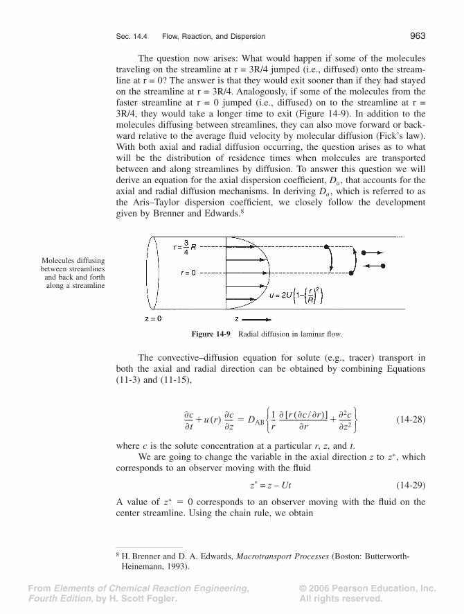
The question now arises: What would happen if some of the moleculestraveling on the streamline at r = 3R/4 jumped (i.e., diffused) onto the stream-line at r = 0? The answer is that they would exit sooner than if they had stayedon the streamline at r = 3R/4. Analogously, if some of the molecules from thefaster streamline at r = 0 jumped (i.e., diffused) on to the streamline at r =3R/4, they would take a longer time to exit (Figure 14-9). In addition to themolecules diffusing between streamlines, they can also move forward or back-ward relative to the average fluid velocity by molecular diffusion (Fick’s law).With both axial and radial diffusion occurring, the question arises as to whatwill be the distribution of residence times when molecules are transportedbetween and along streamlines by diffusion. To answer this question we willderive an equation for the axial dispersion coefficient,
D
a
, that accounts for theaxial and radial diffusion mechanisms. In deriving
D
a
, which is referred to asthe Aris–Taylor dispersion coefficient, we closely follow the developmentgiven by Brenner and Edwards.
8
The convective–diffusion equation for solute (e.g., tracer) transport inboth the axial and radial direction can be obtained by combining Equations(11-3) and (11-15),
(14-28)
where
c
is the solute concentration at a particular
r
,
z
, and
t
.We are going to change the variable in the axial direction
z
to , whichcorresponds to an observer moving with the fluid
z
*
=
z
–
Ut
(14-29)
A value of
�
0 corresponds to an observer moving with the fluid on thecenter streamline. Using the chain rule, we obtain
8
H.
Brenner and D. A. Edwards,
Macrotransport Processes
(Boston: Butterworth-Heinemann, 1993).
Molecules diffusingbetween streamlines
and back and forthalong a streamline
Figure 14-9 Radial diffusion in laminar flow.
�c�t----- u r( ) � c
� z ----- � � D AB 1
r --- � r � c � r � ( )[ ]
� r ------------------------------ �
2
c �
z
2
-------- � Ó ˛Ì ˝Ï ¸
z�
z�

© 2006 Pearson Education, Inc.All rights reserved.
From Elements of Chemical Reaction Engineering,Fourth Edition, by H. Scott Fogler.
964
Models for Nonideal Reactors Chap. 14
(14-30)
Because we want to know the concentrations and conversions at the exit to thereactor, we are really only interested in the average axial concentration ,which is given by
(
z
,
t
)
�
c
(
r
,
z
,
t
)2
�
r dr
(14-31)
Consequently, we are going to solve Equation (14-30) for the solution concen-tration as a function of r and then substitute the solution c (r, z, t) into Equa-tion (14-31) to find (
z
,
t
). All the intermediate steps are given on theCD-ROM R14.1, and the partial differential equation describing the variationof the average axial concentration with time and distance is
(14-32)
where is the Aris–Taylor dispersion coefficient:
(14-33)
That is, for laminar flow in a pipe
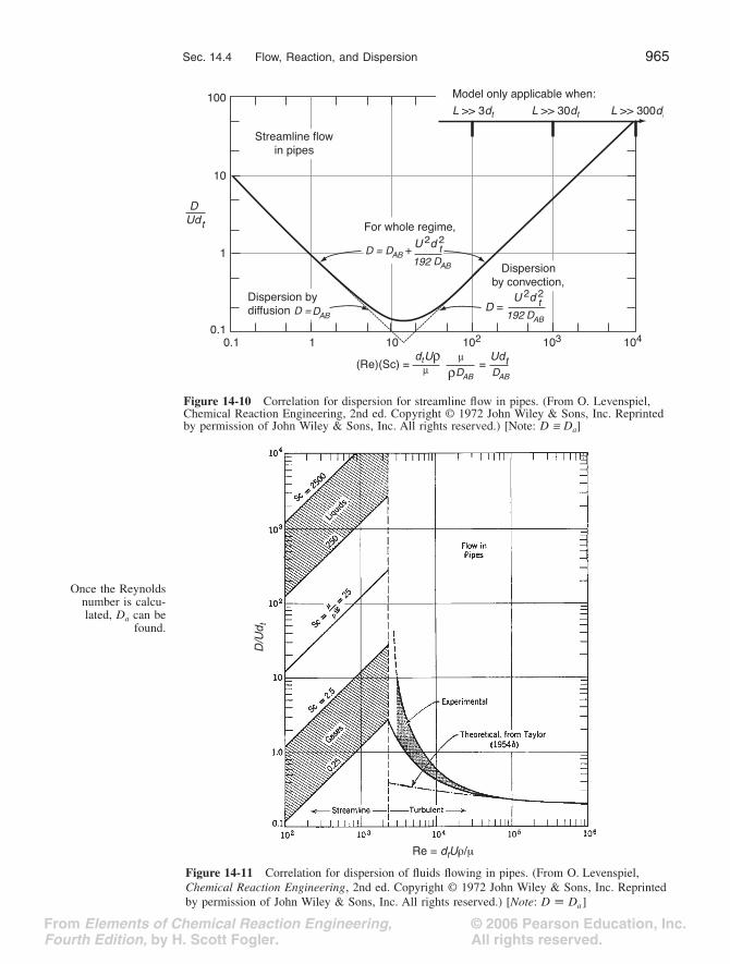
Figure 14-10 shows the dispersion coefficient in terms of the ratio/
U
(2
R
)
�
/
Ud
t
as a function of the product of the Reynolds and Schmidtnumbers.
14.4.5 Correlations for
D
a
14.4.5A Dispersion for Laminar and Turbulent Flow in Pipes
An estimate of the dispersion coefficient,
D
a
, can be determined from Figure14-11. Here d
t
is the tube diameter and Sc is the Schmidt number discussed inChapter 11. The flow is laminar (streamline) below 2,100, and we see the ratio(Da/Udt) increases with increasing Schmidt and Reynolds numbers. BetweenReynolds numbers of 2,100 and 30,000, one can put bounds on Da by calculat-ing the maximum and minimum values at the top and bottom of the shadedregion.
�c�t-----
Ë ¯Á ˜Ê ˆ
z�
u r( ) U�[ ] � c �
z
� ------- � D AB
1 r --- �
� r ----- r � c
�
r -----
Ë ¯Á ˜Ê ˆ
�
2 c
�
z
�
2 --------- ��
C
C 1�R2----------
0
R �
C
�C�t------- U � C
� z
� ------- � D � �
2 C
�
z
� 2 --------- �
D�
Aris–Taylordispersioncoefficient
D� DABU2R2
48DAB----------------��
Da D��
D�
D� D�
© 2006 Pearson Education, Inc.All rights reserved.
From Elements of Chemical Reaction Engineering,Fourth Edition, by H. Scott Fogler.
Sec. 14.4 Flow, Reaction, and Dispersion
965
100
10
1
0.10.1 1 10 102 103 104
DUdt
Streamline flowin pipes
Dispersionby convection,
U 2d 2D = t
For whole regime,
U 2d 2t
(Re)(Sc) = = UdU t
DD =192
192D =
ABDAB
DAB
DABDAB
DAB
Model only applicable when:
L >> 3dt L >> 30dt L >> 300dt
dt
Dispersion bydiffusion
Figure 14-10
Correlation for dispersion for streamline flow in pipes. (From O. Levenspiel,
Chemical Reaction Engineering, 2nd ed. Copyright © 1972 John Wiley & Sons, Inc. Reprinted by permission of John Wiley & Sons, Inc. All rights reserved.) [Note:
D
∫
D
a
]
D/U
d t
Re = dtUρ/μ
Figure 14-11 Correlation for dispersion of fluids flowing in pipes. (From O. Levenspiel, Chemical Reaction Engineering, 2nd ed. Copyright © 1972 John Wiley & Sons, Inc. Reprinted by permission of John Wiley & Sons, Inc. All rights reserved.) [Note: D � Da]
Once the Reynoldsnumber is calcu-lated, Da can be
found.

© 2006 Pearson Education, Inc.All rights reserved.
From Elements of Chemical Reaction Engineering,Fourth Edition, by H. Scott Fogler.
966 Models for Nonideal Reactors Chap. 14
14.4.5B Dispersion in Packed Beds
For the case of gas–solid and liquid–solid catalytic reactions that take place inpacked-bed reactors, the dispersion coefficient, Da, can be estimated by usingFigure 14-12. Here dp is the particle diameter and e is the porosity.
14.4.6 Experimental Determination of Da
The dispersion coefficient can be determined from a pulse tracer experiment.Here, we will use tm and 2 to solve for the dispersion coefficient Da and thenthe Peclet number, Per. Here the effluent concentration of the reactor is mea-sured as a function of time. From the effluent concentration data, the mean res-idence time, tm, and variance, 2, are calculated, and these values are then usedto determine Da. To show how this is accomplished, we will write
(14-13)
in dimensionless form, discuss the different types of boundary conditions atthe reactor entrance and exit, solve for the exit concentration as a function ofdimensionless time (� � t/t), and then relate Da , 2, and t.
14.4.6A The Unsteady-State Tracer Balance
The first step is to put Equation (14-13) in dimensionless form to arrive at thedimensionless group(s) that characterize the process. Let
y � , � , and � �
D/U
d pε
Re = dpUρ/μ
Figure 14-12 Experimental findings on dispersion of fluids flowing with mean axial velocity u in packed beds. (From O. Levenspiel, Chemical Reaction Engineering, 2nd ed. Copyright © 1972 John Wiley & Sons, Inc. Reprinted by permission of John Wiley & Sons, Inc. All rights reserved.) [Note: D � Da]
Da�
2CT
�z2-----------
� UCT( )�z
------------------��CT
�t---------�
CT
CT0
-------- zL--- tU
L------

© 2006 Pearson Education, Inc.All rights reserved.
From Elements of Chemical Reaction Engineering,Fourth Edition, by H. Scott Fogler.
Sec. 14.4 Flow, Reaction, and Dispersion 967
For a pulse input, CT0 is defined as the mass of tracer injected, M, divided bythe vessel volume, V. Then
(14-34)
The initial condition is
At t = 0, z > 0, CT(0+,0) = 0, �(0+)� 0 (14-35)
The mass of tracer injected, M is
M = UAc (0–, t) dt
14.4.6B Solution for a Closed-Closed System
In dimensionless form, the Danckwerts boundary conditions are
At l = 0: (14-36)
At l = 1: (14-37)
Equation (14-34) has been solved numerically for a pulse injection, and theresulting dimensionless effluent tracer concentration, �exit, is shown as a func-tion of the dimensionless time Q in Figure 14-13 for various Peclet numbers.Although analytical solutions for � can be found, the result is an infinite series.The corresponding equations for the mean residence time, tm , and the variance,2, are9
(14-38)
and
(t � t)2E(t) dt
which can be used with the solution to Equation (14-34) to obtain
9 See K. Bischoff and O. Levenspiel, Adv. Chem. Eng., 4, 95 (1963).
1Per
-------- � 2
�
�
2 --------- ��
� ------ �
����
------- �
Initial condition
CT0
�
�
1Per
-------���� ------Ë ¯
Ê ˆ 0�
+� 0+( )�
CT 0 � t,( )CT0
---------------------- 1� �
��� ------ 0�
0 L0+ L+
tm t�
2
tm2
----- 1t2----
0
� �
�

© 2006 Pearson Education, Inc.All rights reserved.
From Elements of Chemical Reaction Engineering,Fourth Edition, by H. Scott Fogler.
968
Models for Nonideal Reactors Chap. 14
(14-39)
Consequently, we see that the Peclet number, Pe
r
(and hence
D
a
), can be foundexperimentally by determining
t
m
and
2
from the RTD data and then solvingEquation (14-39) for Pe
r
.
14.4.6C Open-Open Vessel Boundary Conditions
When a tracer is injected into a packed bed at a location more than two orthree particle diameters downstream from the entrance and measured some dis-tance upstream from the exit, the open-open vessel boundary conditions apply.For an open-open system, an analytical solution to Equation (14-13) can beobtained for a pulse tracer input.
For an open-open system, the boundary conditions at the entrance are
F
T
(0
�
,
t
)
�
F
T
(0
�
,
t
)
10
O. Levenspiel,
Chemical Reaction Engineering
, 2nd ed. (New York: Wiley, 1972),p. 277.
2.0
1.5
1.0
0.5
0 0.5 1.0 1.5 2.0
Mixed flow, DuL
= ∞
Plug flow, DuL
= 0
DuL
= 0.002
Small amount of dispersion,
DuL
= 0.025
Intermediate amount of dispersion,
DuL
= 0.2
Large amount of dispersion,
τ
Figure 14-13 C curves in closed vessels for various extents of back-mixing as predicted by the dispersion model. (From O. Levenspiel, Chemical Reaction Engineering, 2nd ed. Copyright © 1972 John Wiley & Sons, Inc. Reprinted by permission of John Wiley & Sons, Inc. All rights reserved.) [Note: D � Da]10
Calculating Perusing tm and 2
determined fromRTD data for a
closed-closedsystem
2
tm2
----- 2Per
-------- 2Per
2--------- 1 e
Pe
r
� � ( ) ��
Effects ofdispersion on the
effluent tracerconcentration

© 2006 Pearson Education, Inc.All rights reserved.
From Elements of Chemical Reaction Engineering,Fourth Edition, by H. Scott Fogler.
Sec. 14.4 Flow, Reaction, and Dispersion
969
Then for the case when the dispersion coefficient is the same in the entranceand reaction sections:
(14-40)
Because there are no discontinuities across the boundary at
z
= 0
(14-41)
At the exit
(14-42)
(14-43)
There are a number of perturbations of these boundary conditions that can beapplied. The dispersion coefficient can take on different values in each of thethree regions (
z
< 0, 0 <
z
<
L
, and z >
L
), and the tracer can also be injectedat some point
z
1
rather than at the boundary,
z
= 0. These cases and others canbe found in the supplementary readings cited at the end of the chapter. Weshall consider the case when there is no variation in the dispersion coefficientfor all
z
and an impulse of tracer is injected at
z
= 0 at
t
= 0.For long tubes (Pe
r > 100) in which the concentration gradient at ±
•
will be zero, the solution to Equation (14-34) at the exit is 11
(14-44)
The mean residence time for an open-open system is
(14-45)
where
t
is based on the volume between z = 0 and z = L (i.e., reactor volumemeasured with a yardstick). We note that the mean residence time for an opensystem is greater than that for a closed system. The reason is that the mole-cules can diffuse back into the reactor after they diffuse out at the entrance.The variance for an open-open system is
(14-46)
11
W. Jost,
Diffusion in Solids, Liquids and Gases
(New York: Academic Press, 1960),pp. 17, 47.
Da�CT
�z---------Ë ¯
Ê ˆz 0
��
� UCT 0 � t,( )� Da�CT
�z---------Ë ¯
Ê ˆz 0
+�
� UCT 0+ t,( )��
CT 0 � t,( ) CT 0+ t,( )�
Open at the exit Da�CT
�z---------Ë ¯
Ê ˆz L
��
� UCT L � t,( )� Da�CT
�z---------Ë ¯
Ê ˆz L
+�
� UCT L+ t,( )��
CT L � t,( ) CT L+ t,( )�
Valid for Per > 100� 1 �,( ) CT L t,( )
CT0
------------------ 1
2 ��/Per
------------------------- exp 1 ��( )2�
4�/Per
-------------------------� �
Calculate t for anopen-open system
tm 1 2Per
-------�Ë ¯Ê ˆ t�
Calculate Per for anopen–open system.
2
t2----- 2
Per
-------- 8Per
2---------��
© 2006 Pearson Education, Inc.All rights reserved.
From Elements of Chemical Reaction Engineering,Fourth Edition, by H. Scott Fogler.
970 Models for Nonideal Reactors Chap. 14
We now consider two cases for which we can use Equations (14-39) and(14-46) to determine the system parameters:
Case 1. The space time t is known. That is, V and v0 are measuredindependently. Here we can determine the Peclet number bydetermining tm and 2 from the concentration–time data andthen using Equation (14-46) to calculate Per. We can also cal-culate tm and then use Equation (14-45) as a check, but this isusually less accurate.
Case 2. The space time t is unknown. This situation arises when thereare dead or stagnant pockets that exist in the reactor along withthe dispersion effects. To analyze this situation we first calcu-late tm and 2 from the data as in case 1. Then use Equation(14-45) to eliminate t2 from Equation (14-46) to arrive at
(14-47)
We now can solve for the Peclet number in terms of our exper-imentally determined variables 2 and . Knowing Per, wecan solve Equation (14-45) for t, and hence V. The dead vol-ume is the difference between the measured volume (i.e., witha yardstick) and the effective volume calculated from the RTD.
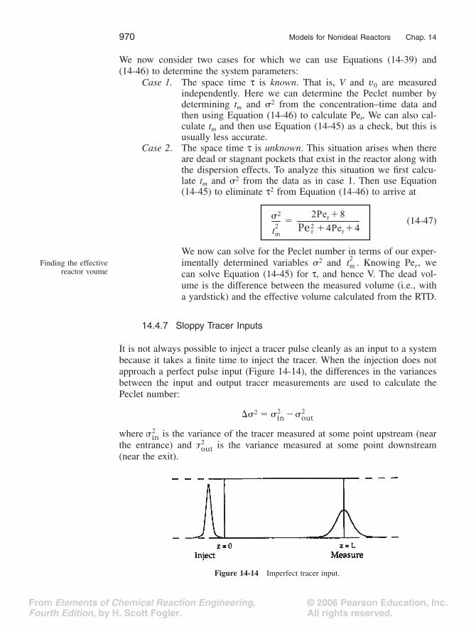
14.4.7 Sloppy Tracer Inputs
It is not always possible to inject a tracer pulse cleanly as an input to a systembecause it takes a finite time to inject the tracer. When the injection does notapproach a perfect pulse input (Figure 14-14), the differences in the variancesbetween the input and output tracer measurements are used to calculate thePeclet number:
where is the variance of the tracer measured at some point upstream (nearthe entrance) and is the variance measured at some point downstream(near the exit).
2
tm2
-----2Per 8�
Pe r2 4Per 4� �
--------------------------------------�
Finding the effectivereactor voume
tm2
�2 in2 out
2��
in2
out2
Figure 14-14 Imperfect tracer input.

© 2006 Pearson Education, Inc.All rights reserved.
From Elements of Chemical Reaction Engineering,Fourth Edition, by H. Scott Fogler.
Sec. 14.4 Flow, Reaction, and Dispersion 971
For an open-open system, it has been shown12 that the Peclet number canbe calculated from the equation
(14-48)
Now let’s put all the material in Section 14.4 together to determine the conver-sion in a tubular reactor for a first-order reaction.
Example 14–2 Conversion Using Dispersion and Tanks-in-Series Models
The first-order reaction
A B
is carried out in a 10-cm-diameter tubular reactor 6.36 m in length. The specificreaction rate is 0.25 min�1. The results of a tracer test carried out on this reactor areshown in Table E14-2.1.
Calculate the conversion using (a) the closed vessel dispersion model, (b) PFR,(c) the tanks-in-series model, and (d) a single CSTR.
Solution
(a) We will use Equation (14-27) to calculate the conversion
(14-27)
where Da � tk, and Per � UL/Da . We can calculate Per fromEquation (14-39):
(14-39)
However, we must find t2 and 2 from the tracer concentration data first.
12R. Aris, Chem. Eng. Sci., 9, 266 (1959).
TABLE E14-2.1. EFFLUENT TRACER CONCENTRATION AS A FUNCTION OF TIME
t (min) 0 1 2 3 4 5 6 7 8 9 10 12 14
C (mg/L) 0 1 5 8 10 8 6 4 3 2.2 1.5 0.6 0
�2
tm2
---------- 2Per
--------�
ææÆ
X 14q Pe r 2 � ( ) exp
1
q
�
( )
2 Pe r q 2 � ( ) 1 q � ( ) 2 P � e r q 2 � ( ) exp � exp ----------------------------------------------------------------------------------------------------------------------------
��
q 1 4DDDDaaaa Per���
2
t2----- 2
Per
-------- 2Per
2--------- 1 e
Pe
r
� � ( ) ��
First calculate tm and2 from RTD data.
t tE t ( ) td
0
� �
V v
---
� �
2 t t � ( ) 2 E t ( ) td
0
� � t 2 E t ( ) t t 2 � d
0
� �
� �
(E14-2.1)( )
(E14-2.2)

© 2006 Pearson Education, Inc.All rights reserved.
From Elements of Chemical Reaction Engineering,Fourth Edition, by H. Scott Fogler.
972
Models for Nonideal Reactors Chap. 14
Consider the data listed in Table E14-2.2.
To find
E
(
t
) and then
t
m
, we first find the area under the
C
curve, which is
Then
Calculating the first term on the right-hand side of Equation (E14-2.2), we find
Substituting these values into Equation (E14-2.2), we obtain the variance,
2
.
Most people, including the author, would use Polymath or Excel to form TableE14-2.2 and to calculate
t
m
and
2
. Dispersion in a closed vessel is represented by
(14-39)
Solving for Pe
r
either by trial and error or using Polymath, we obtain
Pe r � 7.5
Next we calculate
Da
to be
Da
�
t
k
�
(5.15 min)(0.25 min
�
1
)
�
1.29
T
ABLE
E14-2.2.
C
ALCULATIONS
TO
D
ETERMINE
t
m
AND
2
t (min)
0 1 2 3 4 5 6 7 8 9 10 12 14
C(t) (mol/dm3) 0 1 5 8 10 8 6 4 3 2.2 1.5 0.6 0
E(t) (min–1) 0 0.02 0.1 0.16 0.2 0.16 0.12 0.08 0.06 0.044 0.03 0.012 0
tE(t) 0 0.02 0.2 0.48 0.8 0.80 0.72 0.56 0.48 0.400 0.30 0.140 0
t2E(t) (min) 0 0.02 0.4 1.44 3.2 4.0 4.32 3.92 3.84 3.600 3.00 1.680 0
Here againspreadsheets can beused to calculate t2
and 2.
C t ( ) td
0
� �
50 g min
��
t tm tE t ( ) td
0
� �
5.15 min � � �
t 2 E t ( ) td 0
� �
13
---
( )
[1 0
( )
4 0.02
( )
2 0.4
( )
4 1.44
( )
2 3.2
( )
4 4.0
( )
� � � � ��
2 4.32
( )
4 3.92
( )
2 3.84
( )
4 3.6
( )
1 3.0
( )
]
� � � � �
23
---
( )
3.0 4 1.68
( )
0
� �
[ ]
�
32.63 min
2
�
2 32.63 5.15( )2� 6.10 min2� �
Calculate Per fromtm and 2.
2
t2----- 2
Per2
--------- Pe r 1 � e Pe
r
�
� ( ) �
6.15.15
( )
2
-----------------
0.23 2
Pe
r
2
--------- Pe r 1 � e Pe
r
� � ( ) � � �
Next, calculateDa , q, and X.

© 2006 Pearson Education, Inc.All rights reserved.
From Elements of Chemical Reaction Engineering,Fourth Edition, by H. Scott Fogler.
Sec. 14.4 Two-Parameter Models
973
Using the equations for
q
and
X
gives
Then
Substitution into Equation (14-40) yields
When dispersion effects are present in this tubular reactor, 68% conversion isachieved.
(b)
If the reactor were operating ideally as a plug-flow reactor, the conversionwould be
X
�
1
�
e
�
t
k
�
1
�
e
�
Da
�
1
�
e
�
1.29
�
0.725
That is, 72.5% conversion would be achieved in an ideal plug-flow reactor.(c)
Conversion using the tanks-in-series model: We recall Equation (14-12) tocalculate the number of tanks in series:
To calculate the conversion, we recall Equation (4-11). For a first-order reaction for
n
tanks in series, the conversion is
(d)
For a single CSTR,
So 56.3% conversion would be achieved in a single ideal tank.Summary:
In this example, correction for finite dispersion, whether by a dispersion model or atanks-in-series model, is significant when compared with a PFR.
q 1 4DDDDaaaaPer
--------------� 1 4 1.29( )7.5
------------------� 1.30� � �
Per q
2------------ 7.5( ) 1.3( )
2------------------------ 4.87� �
Dispersion ModelX 1 4 1.30( ) e 7.5 2�( )
2.3( )2 4.87 ( ) 0.3 � ( ) 2 4.87 � ( ) exp � exp ------------------------------------------------------------------------------------------------------
��
X
0.68 68% conversion for the dispersion model
�
PFR
Tanks-in-seriesmodel
n t2
2----- 5.15( )2
6.1----------------- 4.35� � �
X 1 11 ti k�( )n
-----------------------� 1 11 t n�( ) k�[ ]n
--------------------------------� 1 11 1.29 4.35��( )4.35
---------------------------------------------�� � �
X 67.7% for the tanks-in-series model�
CSTR X tk1 tk�-------------- 1.29
2.29---------- 0.563� � �
Summary
PFR: X 72.5%�
Dispersion: X 68.0%�
Tanks in series: X 67.7%�
Single CSTR: X 56.3%�

© 2006 Pearson Education, Inc.All rights reserved.
From Elements of Chemical Reaction Engineering,Fourth Edition, by H. Scott Fogler.
974 Models for Nonideal Reactors Chap. 14
14.5 Tanks-in-Series Model Versus Dispersion Model
We have seen that we can apply both of these one-parameter models to tubularreactors using the variance of the RTD. For first-order reactions, the two mod-els can be applied with equal ease. However, the tanks-in-series model is math-ematically easier to use to obtain the effluent concentration and conversion forreaction orders other than one and for multiple reactions. However, we need toask what would be the accuracy of using the tanks-in-series model over thedispersion model. These two models are equivalent when the Peclet–Boden-stein number is related to the number of tanks in series, n, by the equation13
Bo = 2(n – 1) (14-49)
or
(14-50)
where Bo = UL/Da, where U is the superficial velocity, L the reactor length,and Da the dispersion coefficient.
For the conditions in Example 14-2, we see that the number of tanks cal-culated from the Bodenstein number, Bo (i.e., Per), Equation (14-50), is 4.75,which is very close to the value of 4.35 calculated from Equation (14-12).Consequently, for reactions other than first order, one would solve successivelyfor the exit concentration and conversion from each tank in series for both abattery of four tanks in series and of five tanks in series in order to bound theexpected values.
In addition to the one-parameter models of tanks-in-series and disper-sion, many other one-parameter models exist when a combination of idealreactors is used to model the real reactor as shown in Section 13.5 for reactorswith bypassing and dead volume. Another example of a one-parameter modelwould be to model the real reactor as a PFR and a CSTR in series with the oneparameter being the fraction of the total volume that behaves as a CSTR. Wecan dream up many other situations that would alter the behavior of ideal reac-tors in a way that adequately describes a real reactor. However, it may be thatone parameter is not sufficient to yield an adequate comparison between theoryand practice. We explore these situations with combinations of ideal reactors inthe section on two-parameter models.
The reaction rate parameters are usually known (i.e., Da), but the Pecletnumber is usually not known because it depends on the flow and the vessel.Consequently, we need to find Per using one of the three techniques discussedearlier in the chapter.
13K. Elgeti, Chem. Eng. Sci., 51, 5077 (1996).
Equivalencybetween models oftanks-in-series and
dispersion n Bo2
------- 1��
© 2006 Pearson Education, Inc.All rights reserved.
From Elements of Chemical Reaction Engineering,Fourth Edition, by H. Scott Fogler.
Sec. 14.6 Numerical Solutions to Flows with Dispersion and Reaction 975
14.6 Numerical Solutions to Flows with Dispersion and Reaction
We now consider dispersion and reaction. We first write our mole balance onspecies A by recalling Equation (14-28) and including the rate of formation ofA, rA. At steady state we obtain
(14-51)
Analytical solutions to dispersion with reaction can only be obtained for iso-thermal zero- and first-order reactions. We are now going to use COMSOL tosolve the flow with reaction and dispersion with reaction. A COMSOLCD-ROM is included with the text.
We are going to compare two solutions: one which uses the Aris–Taylorapproach and one in which we numerically solve for both the axial and radialconcentration using COMSOL.
Case A. Aris–Taylor Analysis for Laminar Flow
For the case of an nth-order reaction, Equation (14-15) is
(14-52)
If we use the Aris–Taylor analysis, we can use Equation (14-15) with a caveatthat where is the average concentration from r = 0 to r = Ras given by
(14-53)
where
For the closed-closed boundary conditions we have
(14-54)
For the open-open boundary conditions we have
DAB1r---
� r�CA
�r----------Ë ¯
Ê ˆ
�r---------------------
�2CA
�z2------------� u r( )
�CA
�z----------� rA� 0�
Da
U------
d2CA
dz2------------
dCA
dz----------�
kCAn
U---------� 0�
� CA CA0�� CA
1Per
-------d2�
d 2
-------- d�d ------� Da�
n� 0�
PerULDa
------- and Da= tkCA0n 1�
�
At 0:�1
Per
-------d�d ------
0�+
� � 0+( )� 1�
Danckwerts bound-ary conditions At 1:� d�
d ------ 0�
© 2006 Pearson Education, Inc.All rights reserved.
From Elements of Chemical Reaction Engineering,Fourth Edition, by H. Scott Fogler.
976 Models for Nonideal Reactors Chap. 14
(14-55)
Equation (14-53) is a nonlinear second order ODE that is solved on the COMSOLCD-ROM.
Case B. Full Numerical Solution
To obtain profiles, CA(r,z), we now solve Equation (14-51)
(14-51)
First we will put the equations in dimensionless form by letting ,l = z/L, and f = r/R. Following our earlier transformation of variables, Equa-tion (14-51) becomes
(14-56)
Example 14–3 Dispersion with Reaction
(a) First, use COMSOL to solve the dispersion part of Example 14-2 again.How does the COMSOL result compare with the solution to Example 14-2?
(b) Repeat (a) for a second-order reaction with k = 0.5 dm3/mol • min.(c) Repeat (a) but assume laminar flow and consider radial gradients in
concentration. Use DAB for both the radial and axial diffusion coeffi-cients. Plot the axial and radial profiles. Compare your results with part (a).
Additional information:
CA0 = 0.5 mol/dm3, U0 = L/t = 1.24 m/min, Da = U0L/Per = 1.05 m2/min.DAB = 7.6E-5 m2/min.Note: For part (a), the two-dimensional model with no radial gradients (plug flow)becomes a one-dimensional model. The inlet boundary condition for part (a) andpart (b) is a closed-closed vessel (flux[z = 0–] = flux[z = 0+] or Uz·CA0 = flux) at theinlet boundary. In COMSOL format it is: –Ni·n = U0*CA0. The boundary conditionfor laminar flow in COMSOL format for part (c) is: –Ni·n = 2*U0*(1–(r/Ra)2)*CA0.
Solution
(a) Equation (14-52) was used in the COMSOL program along with therate law
At 0:� � 0 �( ) 1Per
-------d�d ------
0� �
� � 0+( ) 1Per
-------d�d ------
0�+
��
At 1:� d�d ------ 0�
DAB1r---
� r�CA
�r----------Ë ¯
Ê ˆ
�r---------------------
�2CA
�z2------------� u r( )
�CA
�z----------� rA� 0�
� CA CA0��
LR---Ë ¯
Ê ˆ 1Per
------- 1�----
� �����-------Ë ¯
Ê ˆ
��------------------- 1
Per
-------d2�
d 2
--------- 2 1 �2
�( )d�d ------� Da�
n�� 0�
The differenttypes of COMSOL
Boundary Conditionsare given in
Problem P14-19c

© 2006 Pearson Education, Inc.All rights reserved.
From Elements of Chemical Reaction Engineering,Fourth Edition, by H. Scott Fogler.
Sec. 14.6 Numerical Solutions to Flows with Dispersion and Reaction 977
rA = –kCA = –kCA0 y
We see that we get the same results as the analytical solution in Exam-ple 14-2. With the Aris–Taylor analysis the two-dimensional profilebecomes a one-dimensional plug flow velocity profile. Figure E14-3.1(a)shows a uniform concentration surface and shows the plug flow behav-ior of the reactor. Figure E14-3.1(b) shows the corresponding cross-sec-tion plots at the inlet, half axial location, and outlet. The average outletconversion is 67.9%.The average outlet concentration at an axial distance z is found by inte-grating across the radius as shown below
From the average concentrations at the inlet and outlet we can calculatethe average conversion as
(b) Now we expand our results to consider the case when the reaction issecond order (–rA = y2) with k = 0.5 dm3/mol·min andCA0 = 0.5 mol/dm3. Let’s assume the radial dispersion coefficient isequal to the molecular diffusivity. Keeping everything else constant, theaverage outlet conversion is 52.3%. However, because the flow insidethe reactor is modeled as plug flow the concentration profiles are stillflat, as shown in Figure E14-3.2.
CA z( ) 2�rCA r z,( )dr
�R2----------------------------------
0
R
��
Be sure to viewdocumentation on
COMSOL CD-ROMto see COMSOL
tutorial withscreen shots X
CA0 CA�
CA0
----------------------�
Figure E14-3.1 COMSOL results for a plug flow reactor with first-order reaction. (Concentrations in mol/dm3.)
(a) (b)
Load enclosedCOMSOL CD
kCA2 kCA0
2�

© 2006 Pearson Education, Inc.All rights reserved.
From Elements of Chemical Reaction Engineering,Fourth Edition, by H. Scott Fogler.
978 Models for Nonideal Reactors Chap. 14
(c) Now, we will change the flow assumption from plug flow to laminarflow and solve Equation (14-51) for a first-order reaction.
The average outlet conversion becomes 68.8%, not much different fromthe one in part (a) in agreement with the Aris–Taylor analysis. How-ever, due to the laminar flow assumption in the reactor, the radial con-centration profiles are very different throughout the reactor.
(d) As a homework exercise, repeat part (c) for the second-order reactiongiven in part (b).
(a) (b)
Figure E14-3.2 COMSOL results for a plug flow reactor with second-order reaction. (Concentrations in mol/dm3.)
Figure E14-3.3 COMSOL output for laminar flow in the reactor. (Concentrations in mol/dm3.)
(a) (b)

© 2006 Pearson Education, Inc.All rights reserved.
From Elements of Chemical Reaction Engineering,Fourth Edition, by H. Scott Fogler.
Sec. 14.7 Two-Parameter Models 979
14.7 Two-Parameter Models—Modeling Real Reactors with Combinationsof Ideal Reactors
We now will see how a real reactor might be modeled by one of two differentcombinations of ideal reactors. These are but two of an almost unlimited num-ber of combinations that could be made. However, if we limit the number ofadjustable parameters to two (e.g., bypass flow rate, vb, and dead volume, VD),the situation becomes much more tractable. After reviewing the steps in Table14-1, choose a model and determine if it is reasonable by qualitatively compar-ing it with the RTD, and if it is, determine the model parameters. Usually, thesimplest means of obtaining the necessary data is some form of tracer test.These tests have been described in Chapter 13, together with their uses indetermining the RTD of a reactor system. Tracer tests can be used to determinethe RTD, which can then be used in a similar manner to determine the suitabil-ity of the model and the value of its parameters.
In determining the suitability of a particular reactor model and theparameter values from tracer tests, it may not be necessary to calculate theRTD function E(t). The model parameters (e.g., VD) may be acquired directlyfrom measurements of effluent concentration in a tracer test. The theoreticalprediction of the particular tracer test in the chosen model system is comparedwith the tracer measurements from the real reactor. The parameters in themodel are chosen so as to obtain the closest possible agreement between themodel and experiment. If the agreement is then sufficiently close, the model isdeemed reasonable. If not, another model must be chosen.
The quality of the agreement necessary to fulfill the criterion “suffi-ciently close” again depends on creativity in developing the model and onengineering judgment. The most extreme demands are that the maximum errorin the prediction not exceed the estimated error in the tracer test and that therebe no observable trends with time in the difference between prediction (themodel) and observation (the real reactor). To illustrate how the modeling iscarried out, we will now consider two different models for a CSTR.
14.7.1 Real CSTR Modeled Using Bypassing and Dead Space
A real CSTR is believed to be modeled as a combination of an ideal CSTR ofvolume Vs , a dead zone of volume Vd , and a bypass with a volumetric flow rate
(Figure 14-15). We have used a tracer experiment to evaluate the parame-ters of the model Vs and . Because the total volume and volumetric flow rateare known, once Vs and are found, and Vd can readily be calculated.
14.7.1A Solving the Model System for CA and X
We shall calculate the conversion for this model for the first-order reaction
A B
Creativity andengineering
judgment arenecessary for model
formulation
A tracerexperiment is used
to evaluate themodel parameters.
vb
vs
vs vb
ææÆ

© 2006 Pearson Education, Inc.All rights reserved.
From Elements of Chemical Reaction Engineering,Fourth Edition, by H. Scott Fogler.
980
Models for Nonideal Reactors Chap. 14
The bypass stream and effluent stream from the reaction volume are mixed atpoint 2. From a balance on species A around this point,
(14-57)
We can solve for the concentration of A leaving the reactor,
Let
�
�
V
s
/
V
and
�
�
. Then
C
A
�
�
C
A0
�
(1
�
�
)
C
A
s
(14-58)
For a first-order reaction, a mole balance on
V
s
gives
C
A0
�
C
A
s
�
kC
A
s
V
s
�
0 (14-59)
or, in terms of
�
and
�
,
(14-60)
Substituting Equation (14-60) into (14-58) gives the effluent concentration ofspecies A:
(14-61)
We have used the ideal reactor system shown in Figure 14-15 to predictthe conversion in the real reactor. The model has two parameters,
�
and
�. Ifthese parameters are known, we can readily predict the conversion. In the fol-lowing section, we shall see how we can use tracer experiments and RTD datato evaluate the model parameters.
Figure 14-15 (a) Real system; (b) model system.
The model system
Balance at junction In[ ] Out[ ]�
CA0vb CAsvs�[ ] CA vb vs�( )[ ]�
CAvbCA0 CAs vs�
vb vs�-----------------------------------
vbCA0 CAs vs�
v0
-----------------------------------� �
vb v0�
Mole balance onCSTR vs vs
CAsCA0 1 ��( ) v0
1 ��( ) v0 �Vk�----------------------------------------�
Conversion as afunction of model
parameters
CACA0
--------- 1 X� �1 ��( )2
1 ��( ) �tk�---------------------------------�� �

© 2006 Pearson Education, Inc.All rights reserved.
From Elements of Chemical Reaction Engineering,Fourth Edition, by H. Scott Fogler.
Sec. 14.7 Two-Parameter Models 981
14.7.1B Using a Tracer to Determine the Model Parameters in CSTR-with-Dead-Space-and-Bypass Model
In Section 14.7.1A, we used the system shown in Figure 14-16, with bypassflow rate and dead volume Vd , to model our real reactor system. We shallinject our tracer, T, as a positive-step input. The unsteady-state balance on thenonreacting tracer T in the reactor volume Vs is
In – out = accumulation
(14-62)
The conditions for the positive-step input are
A balance around junction point 2 gives
(14-63)
As before,
Integrating Equation (14-62) and substituting in terms of � and � gives
(14-64)
vb
Tracer balance forstep input vsCT0 � v s C Ts �
dN
Ts dt ----------- V s
dC
Ts dt ----------- �
CT0
CT0
CT
CTS
1
2
v0
v0
v0v
v0 v v
v
Figure 14-16 Model system: CSTR with dead volume and bypassing.
Model system
At t 0�
At t 0�
CT 0�
CT CT0�
The junctionbalance
CTvbCT0 CTsvs�
v0
---------------------------------�
Vs �V�
vb �v0�
t Vv0
-----�
CTs
CT0
-------- 11 ��
�-------------
t t --
Ë ¯Á ˜Ê ˆ
� exp ��

© 2006 Pearson Education, Inc.All rights reserved.
From Elements of Chemical Reaction Engineering,Fourth Edition, by H. Scott Fogler.
982
Models for Nonideal Reactors Chap. 14
Combining Equations (14-63) and (14-64), the effluent tracer concentration is
(14-65)
We now need to rearrange this equation to extract the model parameters,
a
and
b
, either by regression (Polymath/MATLAB/Excel) or from the proper plot ofthe effluent tracer concentration as a function of time. Rearranging yields
(14-66)
Consequently, we plot ln[
C
T
0
/(
C
T
0
�
C
T
)] as a function of
t
. If ourmodel is correct, a straight line should result with a slope of (1
�
�
)/
t
�
andan intercept of ln[1/(1
�
�
)].
Example 14–4 CSTR with Dead Space and Bypass
The elementary reaction
A
�
B C
�
D
is to be carried out in the CSTR shown schematically in Figure 14-15. There is bothbypassing and a stagnant region in this reactor. The tracer output for this reactor isshown in Table E14-4.1. The measured reactor volume is 1.0 m
3
and the flow rate tothe reactor is 0.1 m
3
/min. The reaction rate constant is 0.28 m
3
/kmol
�
min. The feedis equimolar in A and B with an entering concentration of A equal to 2.0 kmol/m
3
.Calculate the conversion that can be expected in this reactor (Figure E14-4.1).
The entering tracer concentration is C
T0 = 2000 mg/dm3.
TABLE E14-4.1 TRACER DATA FOR STEP INPUT
CT (mg/dm3) 1000 1333 1500 1666 1750 1800
t (min) 4 8 10 14 16 18
CT
CT0
-------- 1 1 ��( ) 1
���
------------- t
t --
Ë ¯Á ˜Ê ˆ
� exp ��
Evaluating themodel parameters
CT0
CT0 CT�---------------------ln 1
1 ��------------- 1 ��
�-------------
Ë ¯Á ˜Ê ˆ
t t -- � ln�
ææÆ
Two-parametermodel
CT0
CA0
v0
v0
vb
CTS
CT
VS
CA
CAS
2
1 0
Figure E14-4.1 Schematic of real reactor modeled with dead space (Vd) and bypass .vb( )

© 2006 Pearson Education, Inc.All rights reserved.
From Elements of Chemical Reaction Engineering,Fourth Edition, by H. Scott Fogler.
Sec. 14.7 Two-Parameter Models
983
Solution
Recalling Equation (14-66)
(14-66)
Equation (14-66) suggests that we construct Table E14-4.2 from Table E14-4.1 andplot
C
T
0
/(
C
T
0
�
C
T
) as a function of time on semilog paper. Using this table we getFigure E14-4.2.
We can find
a
and
b
from either a semilog plot as shown in Figure E14-4.2 or byregression using Polymath, MATLAB, or Excel.
The volumetric flow rate to the well-mixed portion of the reactor, , can be deter-mined from the intercept,
I
:
The volume of the well-mixed region,
V
s
, can be calculated from the slope:
T
ABLE
E14-4.2.
P
ROCESSED
D
ATA
t
(min) 4 8 10 14 16 18
2 3 4 6 8 10
CT0
CT0 CT�---------------------ln 1
1 ��------------- 1 ��( )
�----------------- t
t--�ln�
Evaluating theparameters � and �
CT0
CT0 CT�---------------------
Figure E14-4.2 Response to a step input.
vs
11 ��------------- I 1.25� �
�vb
v0
----- 0.2� �
1 ���t
------------- S 0.115 min 1�� �
�t 1 0.2�0.115
----------------- 7 min� �

© 2006 Pearson Education, Inc.All rights reserved.
From Elements of Chemical Reaction Engineering,Fourth Edition, by H. Scott Fogler.
984 Models for Nonideal Reactors Chap. 14
We now proceed to determine the conversion corresponding to these model parameters.1. Balance on reactor volume Vs:
(E14-4.1)
2. Rate law:
Equimolar feed
(E14-4.2)
3. Combining Equations (E14-4.1) and (E14-4.2) gives
(E14-4.3)
Rearranging, we have
� CAs � CA0 � 0 (E14-4.4)
Solving for CAs yields
(E14-4.5)
4. Balance around junction point 2:
(E14-4.6)
Rearranging Equation (E14-4.6) gives us
(E14-4.7)
t Vv0
----- 1 m3
0.1 m3/min( )------------------------------- 10 min� � �
� 7 mint
-------------- 0.7� �
In[ ] Out + Generation = Accumulation�
vsCA0 vsCAs� rAsVs� 0�
rAS� kCAsCBs�
CAs� CBs�
rAs kC 2As��
vs CA0 vs CAs� kCAs2 Vs� 0�
ts kCAs2
The Duck TapeCouncil would like
to point out thenew wrinkle: The
Junction Balance. CAs1� 1 4ts kCA0��
2ts k-------------------------------------------------�
In[ ] Out[ ]�
vbCA0 vsCAs�[ ] v0CA[ ]�
CAv0 vs�
v0
---------------- C A 0 v
s
v
0
----- C A s ��
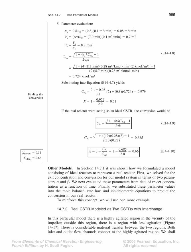
© 2006 Pearson Education, Inc.All rights reserved.
From Elements of Chemical Reaction Engineering,Fourth Edition, by H. Scott Fogler.
Sec. 14.7 Two-Parameter Models
985
5. Parameter evaluation:
(E14-4.8)
Substituting into Equation (E14-4.7) yields
If the real reactor were acting as an ideal CSTR, the conversion would be
(E14-4.9)
(E14-4.10)
Other Models.
In Section 14.7.1 it was shown how we formulated a modelconsisting of ideal reactors to represent a real reactor. First, we solved for theexit concentration and conversion for our model system in terms of two param-eters � and � . We next evaluated these parameters from data of tracer concen-tration as a function of time. Finally, we substituted these parameter valuesinto the mole balance, rate law, and stoichiometric equations to predict theconversion in our real reactor.
To reinforce this concept, we will use one more example.
14.7.2 Real CSTR Modeled as Two CSTRs with Interchange
In this particular model there is a highly agitated region in the vicinity of theimpeller; outside this region, there is a region with less agitation (Figure14-17). There is considerable material transfer between the two regions. Bothinlet and outlet flow channels connect to the highly agitated region. We shall
vs 0.8 v0 0.8( ) 0.1 m3 min�( ) 0.08 m3 min�� � �
Vs �t( ) v0 7.0 min( ) 0.1 m3 min�( ) 0.7 m3� � �
tsVs
vs
----- 8.7 min� �
CAs1 4ts kCA0� 1�
2ts k-------------------------------------------�
1 4( ) 8.7 min( ) 0.28 m3 kmol min��( ) 2 kmol m3�( )� 1�
2( ) 8.7 min( ) 0.28 m3 kmol min��( )------------------------------------------------------------------------------------------------------------------------------------------�
0.724 kmol m3��
Finding theconversion
CA0.1 0.08�
0.1------------------------ 2 ( ) 0.8 ( ) 0.724 ( ) � 0.979 � �
X
1 0.9792.0
-------------
�
0.51
� �
CA1 4tkCA0� 1�
2tk-----------------------------------------�
CA1 4 10( ) 0.28( ) 2( )� 1�
2 10( ) 0.28( )----------------------------------------------------------- 0.685� �
Xmodel 0.51�
XIdeal 0.66�
X 1CACA0
---------� 1 0.6852.0
-------------� 0.66� � �

© 2006 Pearson Education, Inc.All rights reserved.
From Elements of Chemical Reaction Engineering,Fourth Edition, by H. Scott Fogler.
986
Models for Nonideal Reactors Chap. 14
model the highly agitated region as one CSTR, the quieter region as anotherCSTR, with material transfer between the two.
14.7.2A Solving the Model System for
C
A
and
X
Let
�
represent that fraction of the total flow that is exchanged between reac-tors 1 and 2, that is,
and let
�
represent that fraction of the total volume
V occupied by the highlyagitated region:
Then
The space time is
As shown on the CD-ROM 14R.2, for a first-order reaction, the exit concentra-tion and conversion are
(14-67)
and
The model system
(a) (b)
V1V2
CA1
CA1
CA2
v0
v
v
v
Figure 14-17 (a) Real reaction system; (b) model reaction system.
v1 �v0�
Two parameters:� and �
V1 �V�
V2 1 ��( )V�
t Vv0
-----�
CA1CA0
1 � �tk �2 � 1 ��( ) tk�[ ]�{ }�� �----------------------------------------------------------------------------------------�

© 2006 Pearson Education, Inc.All rights reserved.
From Elements of Chemical Reaction Engineering,Fourth Edition, by H. Scott Fogler.
Sec. 14.7 Two-Parameter Models 987
(14-68)
where CA1 is the reactor concentration exiting the first reactor in Figure 14-17(b).
14.7.2B Using a Tracer to Determine the Model Parameters in a CSTR with an Exchange Volume
The problem now is to evaluate the parameters � and � using the RTD data. Amole balance on a tracer pulse injected at t � 0 for each of the tanks is
(14-69)
CT1 and CT2 are the tracer concentrations in reactors 1 and 2, respectively, withinitial conditions CT10 � NT0/V1 and CT20 � 0.
Substituting in terms of �, �, and t, we arrive at two coupled differentialequations describing the unsteady behavior of the tracer that must be solvedsimultaneously.
Analytical solutions to Equations (14-71) and (14-72) are given in theCD-ROM, in Appendix A.3 and in Equation (14-73), below. However, formore complicated systems, analytical solutions to evaluate the system parame-ters may not be possible.
(14-73)
By regression on Equation (14-73) and the data in Table E14-4.2 or by anappropriate semilog plot of CT1/CT10 versus time, one can evaluate the modelparameters � and �.
Conversion fortwo-CSTR model
X 1CA1
CA0
---------�� �tk�( ) � 1 ��( ) tk�[ ] �2�
1 � �tk� �( ) � 1 ��( ) tk�[ ] �2�----------------------------------------------------------------------------------� �
Unsteady-statebalance of inert
tracer
Reactor 1:
Reactor 2:
Accumulation Rate in Rate out��
V1 dC
T
1 dt ----------- v 1 C T 2 v 0 C T 1 v 1 C T 1 � ( ) ��
V
2 dC
T
2 dt ----------- v 1 C T 1 v 1 C T 2 �� 14-70( )
See Appendix A.3for method of
solution
t� dC
T
1 dt ----------- � C T 2 1 �� ( ) C T 1 ��
t
1
��
( ) dC
T
2 dt ----------- � C T 1 � C T 2 ��
14-71( )
14-72( )
CT1
CT10
----------Ë ¯Á ˜Ê ˆ
pulse
�m1 � 1� �( ) em2 t t��m2 � 1� �( ) em1 t t�
�
� m1 m2�( )------------------------------------------------------------------------------------------------------�
where
m1 m 2 , 1 �� �� 2
�
1
��
( )
------------------------- 1 � 1 4 �� 1 �� ( ) 1
�� �
2
�
( )
----------------------------- ���
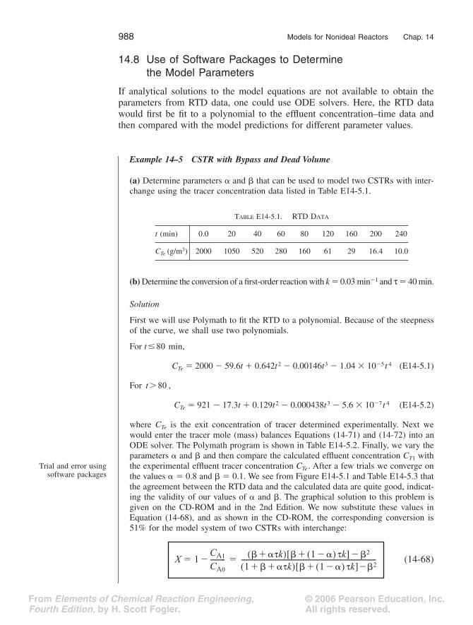
© 2006 Pearson Education, Inc.All rights reserved.
From Elements of Chemical Reaction Engineering,Fourth Edition, by H. Scott Fogler.
988
Models for Nonideal Reactors Chap. 14
14.8 Use of Software Packages to Determine the Model Parameters
If analytical solutions to the model equations are not available to obtain theparameters from RTD data, one could use ODE solvers. Here, the RTD datawould first be fit to a polynomial to the effluent concentration–time data andthen compared with the model predictions for different parameter values.
Example 14–5 CSTR with Bypass and Dead Volume
(a)
Determine parameters
�
and
�
that can be used to model two CSTRs with inter-change using the tracer concentration data listed in Table E14-5.1.
(b)
Determine the conversion of a first-order reaction with
k
�
0.03 min
�
1
and
t
�
40 min.
Solution
First we will use Polymath to fit the RTD to a polynomial. Because of the steepnessof the curve, we shall use two polynomials.
For min,
C
Te
�
2000
�
59.6
t
�
0.642
t
2
�
0.00146
t
3
�
1.04
�
10
�
5
t
4
(E14-5.1)
For ,
C
Te
�
921
�
17.3
t
� 0.129t2 � 0.000438t3 � 5.6 � 10�7 t 4 (E14-5.2)
where CTe is the exit concentration of tracer determined experimentally. Next wewould enter the tracer mole (mass) balances Equations (14-71) and (14-72) into anODE solver. The Polymath program is shown in Table E14-5.2. Finally, we vary theparameters � and � and then compare the calculated effluent concentration CT1 withthe experimental effluent tracer concentration CTe . After a few trials we converge onthe values � � 0.8 and � � 0.1. We see from Figure E14-5.1 and Table E14-5.3 thatthe agreement between the RTD data and the calculated data are quite good, indicat-ing the validity of our values of � and �. The graphical solution to this problem isgiven on the CD-ROM and in the 2nd Edition. We now substitute these values inEquation (14-68), and as shown in the CD-ROM, the corresponding conversion is51% for the model system of two CSTRs with interchange:
(14-68)
TABLE E14-5.1. RTD DATA
t (min) 0.0 20 40 60 80 120 160 200 240
CTe (g/m3) 2000 1050 520 280 160 61 29 16.4 10.0
t 80�
t 80�
Trial and error usingsoftware packages
X 1CA1
CA0
---------�� �tk�( ) � 1 ��( ) tk�[ ] �2�
1 � �tk� �( ) � 1 ��( ) tk�[ ] �2�----------------------------------------------------------------------------------� �
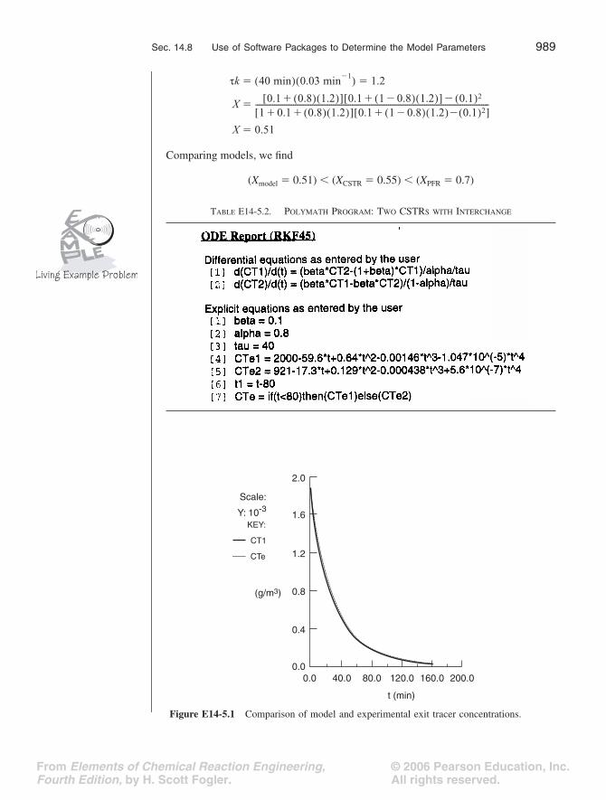
© 2006 Pearson Education, Inc.All rights reserved.
From Elements of Chemical Reaction Engineering,Fourth Edition, by H. Scott Fogler.
Sec. 14.8 Use of Software Packages to Determine the Model Parameters 989
Comparing models, we find
(Xmodel � 0.51) � (XCSTR � 0.55) � (XPFR � 0.7)
TABLE E14-5.2. POLYMATH PROGRAM: TWO CSTRS WITH INTERCHANGE
tk 40 min( ) 0.03 min 1�( ) 1.2� �
X 0.1 0.8( ) 1.2( )�[ ] 0.1 1 0.8�( ) 1.2( )�[ ] 0.1( )2�
1 0.1 0.8( ) 1.2( )� �[ ] 0.1 1 0.8�( ) 1.2( ) 0.1( )2��[ ]---------------------------------------------------------------------------------------------------------------------------�
X 0.51�
2.0
1.6
0.8
0.4
Scale:
Y: 10-3
KEY:
CT1
CTe 1.2
0.00.0 40.0
t (min)
80.0 120.0 160.0 200.0
(g/m3)
Figure E14-5.1 Comparison of model and experimental exit tracer concentrations.

© 2006 Pearson Education, Inc.All rights reserved.
From Elements of Chemical Reaction Engineering,Fourth Edition, by H. Scott Fogler.
990 Models for Nonideal Reactors Chap. 14
14.9 Other Models of Nonideal Reactors Using CSTRs and PFRs
Several reactor models have been discussed in the preceding pages. All arebased on the physical observation that in almost all agitated tank reactors,there is a well-mixed zone in the vicinity of the agitator. This zone is usuallyrepresented by a CSTR. The region outside this well-mixed zone may then bemodeled in various fashions. We have already considered the simplest models,which have the main CSTR combined with a dead-space volume; if someshort-circuiting of the feed to the outlet is suspected, a bypass stream can beadded. The next step is to look at all possible combinations that we can use tomodel a nonideal reactor using only CSTRs, PFRs, dead volume, and bypass-ing. The rate of transfer between the two reactors is one of the model parame-ters. The positions of the inlet and outlet to the model reactor system dependon the physical layout of the real reactor.
Figure 14-18(a) describes a real PFR or PBR with channeling that ismodeled as two PFRs/PBRs in parallel. The two parameters are the fraction offlow to the reactors [i.e., � and (1 � �)] and the fractional volume [i.e., � and(1 � �)] of each reactor. Figure 14-18(b) describes a real PFR/PBR that has abackmix region and is modeled as a PFR/PBR in parallel with a CSTR. Fig-ures 14-19(a) and (b) show a real CSTR modeled as two CSTRs with inter-change. In one case, the fluid exits from the top CSTR (a) and in the other casethe fluid exits from the bottom CSTR. The parameter � represents the inter-change volumetric flow rate and � the fractional volume of the top reactor,where the fluid exits the reaction system. We note that the reactor in model14-19(b) was found to describe extremely well a real reactor used in the pro-duction of terephthalic acid.14 A number of other combinations of ideal reac-tions can be found in Levenspiel.15
14Proc. Indian Inst. Chem. Eng. Golden Jubilee, a Congress, Delhi, 1997, p. 323.15Levenspiel, O. Chemical Reaction Engineering, 3rd ed. (New York: Wiley, 1999),
pp. 284–292.
TABLE E14-5.3. COMPARING MODEL (CT1) WITH EXPERIMENT (CTe)
Two CSTRs withinterchange
A case history forterephthalic acid

© 2006 Pearson Education, Inc.All rights reserved.
From Elements of Chemical Reaction Engineering,Fourth Edition, by H. Scott Fogler.
Sec. 14.10 Applications to Pharmacokinetic Modeling 991
14.10 Applications to Pharmacokinetic Modeling
The use of combinations of ideal reactors to model metabolism and drug distri-bution in the human body is becoming commonplace. For example, one of thesimplest models for drug adsorption and elimination is similar to that shown inFigure 14-19(a). The drug is injected intravenously into a central compartmentcontaining the blood (the top reactor). The blood distributes the drug back andforth to the tissue compartment (the bottom reactor) before being eliminated(top reactor). This model will give the familiar linear semi-log plot found inpharmacokinetics textbooks. As can be seen in the figure for Professional Ref-erence Shelf R7.5 on pharmacokinetics on page 453, there are two differentslopes, one for the drug distribution phase and one for the elmination phase.More elaborate models using combinations of ideal reactors to model a realsystem are described in section 7.5 where alcohol metabolism is discussed.
Model SystemReal System
E F
(a)
v0v0
v0
v0
Model SystemReal System
E(t) F(t)
(b)
}
v0
v0
v0
v0
Figure 14-18 Combinations of ideal reactors used to model real tubular reactors.(a) two ideal PFRs in parallel (b) ideal PFR and ideal CSTR in parallel.

© 2006 Pearson Education, Inc.All rights reserved.
From Elements of Chemical Reaction Engineering,Fourth Edition, by H. Scott Fogler.
992 Models for Nonideal Reactors Chap. 14
Model
E(t) F(t)
t t
(a)
V
Model
E(t) F(t)
t t
(b)
V
v0
v0
v0
v0
βv0 βv0
v0
v0
v0
v0
βv0v0
Figure 14-19 Combinations of ideal reactors to model a real CSTR. Two ideal CSTRs with interchange (a) exit from the top of the CSTR (b) exit from the bottom of the CSTR.
Closure
In this chapter, models were developed for existing reactors to obtain a moreprecise estimate of the exit conversion and concentration than estimates ofthe examples given by the zero-order parameter models of segregation andmaximum mixedness. After completing this chapter, the reader will use theRTD data and kinetic rate law and reactor model to make predictions of theconversion and exit concentrations using the tank-in-series and dispersionone-parameter models. In addition, the reader should be able to create com-binations of ideal reactors that mimic the RTD data and to solve for the exitconversions and concentrations. The choice of a proper model is almost pureart requiring creativity and engineering judgment. The flow pattern of themodel must possess the most important characteristics of that in the realreactor. Standard models are available that have been used with some suc-cess, and these can be used as starting points. Models of real reactors usuallyconsist of combinations of PFRs, perfectly mixed CSTRs, and dead spaces ina configuration that matches the flow patterns in the reactor. For tubular reac-tors, the simple dispersion model has proven most popular.
The parameters in the model, which with rare exception should notexceed two in number, are obtained from the RTD data. Once the parame-ters are evaluated, the conversion in the model, and thus in the real reactor,can be calculated. For typical tank-reactor models, this is the conversion ina series–parallel reactor system. For the dispersion model, the second-orderdifferential equation must be solved, usually numerically. Analytical solu-tions exist for first-order reactions, but as pointed out previously, no modelhas to be assumed for the first-order system if the RTD is available.
Correlations exist for the amount of dispersion that might be expectedin common packed-bed reactors, so these systems can be designed using thedispersion model without obtaining or estimating the RTD. This situation isperhaps the only one where an RTD is not necessary for designing a non-ideal reactor.
RTD Data + Kinetics + Model = Prediction

© 2006 Pearson Education, Inc.All rights reserved.
From Elements of Chemical Reaction Engineering,Fourth Edition, by H. Scott Fogler.
Chap. 14 Summary 993
S U M M A R Y
1. The models for predicting conversion from RTD data are:a. Zero adjustable parameters
(1) Segregation model(2) Maximum mixedness model
b. One adjustable parameter(1) Tanks-in-series model(2) Dispersion model
c. Two adjustable parameters: real reactor modeled as combinations of idealreactors
2. Tanks-in-series model: Use RTD data to estimate the number of tanks inseries,
(S14-1)
For a first-order reaction
X � 1 �
3. Dispersion model: For a first-order reaction, use the Danckwerts boundaryconditions
(S14-2)
where
(S14-3)
Da � tk Per � Pe f � (S14-4)
4. Determine Da
a. For laminar flow the dispersion coefficient is
(S14-5)
b. Correlations. Use Figures 14-10 through 14-12.c. Experiment in RTD analysis to find tm and .For a closed-closed system use Equation (S14-6) to calculate Per from theRTD data:
(S14-6)
The models
n t2
2-----�
11 ti k�( )n
-----------------------
X 14q Pe r 2 � ( ) exp
1
q
�
( )
2 Pe r q 2 � ( ) 1 q � ( ) 2 P � e r q 2 � ( ) exp � exp ----------------------------------------------------------------------------------------------------------------------------
��
q 1 4DaPer
----------��
ULDa
-------Udp
Da �----------
D� DABU2R2
48DAB----------------��
2
2
t2----- 2
Per
-------- 2Per
2--------- 1 e
Pe
r
� � ( ) ��

© 2006 Pearson Education, Inc.All rights reserved.
From Elements of Chemical Reaction Engineering,Fourth Edition, by H. Scott Fogler.
994
Models for Nonideal Reactors Chap. 14
For an open-open system, use
(14-47)
5. If a real reactor is modeled as a combination of ideal reactors, the modelshould have at most two parameters.
6. The RTD is used to extract model parameters.7. Comparison of conversions for a PFR and CSTR with the zero-parameter and
two-parameter models.
X
seg
symbolizes the conversion obtained from the seg-regation model and
X
mm
that from the maximum mixedness model for reac-tion orders greater than one.
Cautions:
For rate laws with unusual concentration functionalities or fornonisothermal operation, these bounds may not be accurate for certain typesof rate laws.
C D - R O M M A T E R I A L
• Learning Resources
1. Summary Notes2. Web Material
COMSOL CD-ROM
• Living Example Problems
1. Example 14-3 Dispersion with Reaction—COMSOL2. Example 14-5 CSTR with Bypass and Dead Volume
2
tm2
-----2Per 8�
Per2 4Per 4� �
----------------------------------�
VS
vS
vb
v0 v0
v0
v1
v2
v0
VD
VI VII
CSTR with bypass and dead volume
Two CSTRs with interchange
XPFR Xseg Xmm XCSTR� � �
XPFR Xmodel with Xmodel XCSTR or Xmodel XCSTR���

© 2006 Pearson Education, Inc.All rights reserved.
From Elements of Chemical Reaction Engineering,Fourth Edition, by H. Scott Fogler.
Chap. 14 CD-ROM Material 995
• Professional Reference ShelfR14.1 Derivation of Equation for Taylor–Aris Dispersion
R14.2 Real Reactor Modeled as two Ideal CSTRs with Exchange VolumeExample R14-1 Two CSTRs with interchange.
COMSOL results
�C�t------- U�C
�z*------- D*
��
2C
�z*2---------�
D* DAB� U2R2
48DAB
----------------�
CA1
CA1
CA2
v0
v0
v1
v1
V V1
2
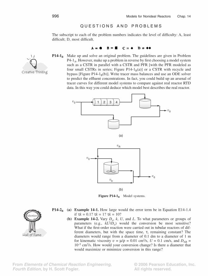
© 2006 Pearson Education, Inc.All rights reserved.
From Elements of Chemical Reaction Engineering,Fourth Edition, by H. Scott Fogler.
996 Models for Nonideal Reactors Chap. 14
Q U E S T I O N S A N D P R O B L E M S
The subscript to each of the problem numbers indicates the level of difficulty: A, leastdifficult; D, most difficult.
P14-1B Make up and solve an original problem. The guidelines are given in ProblemP4-1A. However, make up a problem in reverse by first choosing a model systemsuch as a CSTR in parallel with a CSTR and PFR [with the PFR modeled asfour small CSTRs in series; Figure P14-1B(a)] or a CSTR with recycle andbypass [Figure P14-1B(b)]. Write tracer mass balances and use an ODE solverto predict the effluent concentrations. In fact, you could build up an arsenal oftracer curves for different model systems to compare against real reactor RTDdata. In this way you could deduce which model best describes the real reactor.
P14-2B (a) Example 14-1. How large would the error term be in Equation E14-1.4if tk = 0.1? tk = 1? tk = 10?
(b) Example 14-2. Vary Da, k, U, and L. To what parameters or groups ofparameters (e.g., kL2/Da) would the conversion be most sensitive?What if the first-order reaction were carried out in tubular reactors of dif-ferent diameters, but with the space time, t, remaining constant? Thediameters would range from a diameter of 0.1 dm to a diameter of 1 mfor kinematic viscosity v = m/r = 0.01 cm2/s, U = 0.1 cm/s, and DAB =10–5 cm2/s. How would your conversion change? Is there a diameter thatwould maximize or minimize conversion in this range?
(a)
1 2 3 4
(b)
v0
v0
vR
v0
v0
vb
Figure P14-1B Model systems.

© 2006 Pearson Education, Inc.All rights reserved.
From Elements of Chemical Reaction Engineering,Fourth Edition, by H. Scott Fogler.
Chap. 14 Questions and Problems 997
(c) Example 14-3. (1) Load the reaction and dispersion program from theCOMSOL CD-ROM. Vary the Damköhler number for a second-orderreaction using the Aris–Taylor approximation (part (b) in Example 14-3).(2) Vary the Peclet and Damköhler numbers for a second-order reactionin laminar flow. What values of the Peclet number affect the conversionsignificantly?
(d) Example 14-4. How would your answers change if the slope was 4 min–1
and the intercept was 2 in Figure E14-4.2?(e) Example 14-5. Load the Living Example Polymath Program. Vary a and
b and describe what you find. What would be the conversion if a = 0.75and b = 0.15?
(f) What if you were asked to design a tubular vessel that would minimizedispersion? What would be your guidelines? How would you maximizethe dispersion? How would your design change for a packed bed?
(g) What if someone suggested you could use the solution to the flow-disper-sion-reactor equation, Equation (14-27), for a second-order equation bylinearizing the rate law by lettering –rA = @ (kCA0/2) CA = ?Under what circumstances might this be a good approximation? Wouldyou divide CA0 by something other than 2? What do you think of linear-izing other non-first-order reactions and using Equation (14-27)? Howcould you test your results to learn if the approximation is justified?
(h) What if you were asked to explain why physically the shapes of thecurves in Figure 14-3 look the way they do, what would you say? Whatif the first pulse in Figure 14.1(b) broke through at � � 0.5 and the sec-ond pulse broke through at � � 1.5 in a tubular reactor in which asecond-order liquid-phase reaction
2A B � C
was occurring? What would the conversion be if t � 5 min, CA0 � 2mol/dm3, and k � 0.1 dm3/mol�min?
P14-3B The second-order liquid-phase reaction
A B � C
is to be carried out isothermally. The entering concentration of A is 1.0 mol/dm3.The specific reaction rate is 1.0 dm3/mol�min. A number of used reactors (shownbelow) are available, each of which has been characterized by an RTD. There aretwo crimson and white reactors and three maize and blue reactors available.
(a) You have $50,000 available to spend. What is the greatest conversion youcan achieve with the available money and reactors?
(b) How would your answer to (a) change if you had $75,000 available tospend?
(c) From which cities do you think the various used reactors came from?
Reactor (min) (min) Cost
Maize and blue 2 2 $25,000Green and white 4 4 50,000Scarlet and gray 3.05 4 50,000Orange and blue 2.31 4 50,000Purple and white 5.17 4 50,000Silver and black 2.5 4 50,000Crimson and white 2.5 2 25,000
kCA2 kCA
ææÆ
ææÆ
t
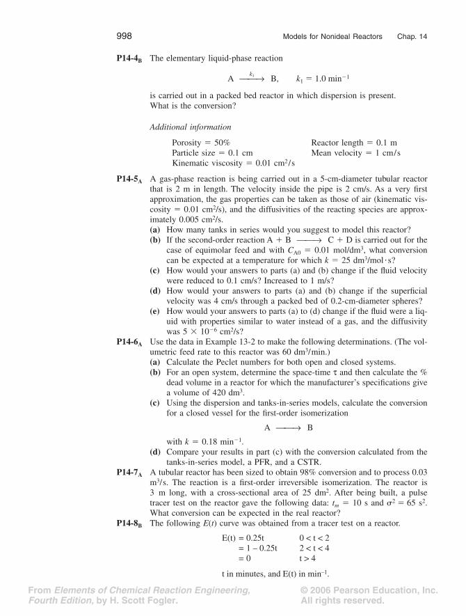
© 2006 Pearson Education, Inc.All rights reserved.
From Elements of Chemical Reaction Engineering,Fourth Edition, by H. Scott Fogler.
998
Models for Nonideal Reactors Chap. 14
P14-4
B
The elementary liquid-phase reaction
A B,
k
1
�
1.0 min
�
1
is carried out in a packed bed reactor in which dispersion is present.What is the conversion?
Additional information
Porosity
�
50% Reactor length
�
0.1 mParticle size
�
0.1 cm Mean velocity
�
1 cm/sKinematic viscosity
�
0.01 cm
2
/s
P14-5
A
A gas-phase reaction is being carried out in a 5-cm-diameter tubular reactorthat is 2 m in length. The velocity inside the pipe is 2 cm/s. As a very firstapproximation, the gas properties can be taken as those of air (kinematic vis-cosity
�
0.01 cm
2
/s), and the diffusivities of the reacting species are approx-imately 0.005 cm
2
/s.
(a)
How many tanks in series would you suggest to model this reactor?
(b)
If the second-order reaction A
�
B C
�
D is carried out for thecase of equimolar feed and with
C
A0
�
0.01 mol/dm
3
, what conversioncan be expected at a temperature for which
k
�
25 dm
3
/mol
�
s?
(c)
How would your answers to parts (a) and (b) change if the fluid velocitywere reduced to 0.1 cm/s? Increased to 1 m/s?
(d)
How would your answers to parts (a) and (b) change if the superficialvelocity was 4 cm/s through a packed bed of 0.2-cm-diameter spheres?
(e)
How would your answers to parts (a) to (d) change if the fluid were a liq-uid with properties similar to water instead of a gas, and the diffusivitywas 5
�
10�6 cm2/s?P14-6A Use the data in Example 13-2 to make the following determinations. (The vol-
umetric feed rate to this reactor was 60 dm3/min.)(a) Calculate the Peclet numbers for both open and closed systems.(b) For an open system, determine the space-time t and then calculate the %
dead volume in a reactor for which the manufacturer’s specifications givea volume of 420 dm3.
(c) Using the dispersion and tanks-in-series models, calculate the conversionfor a closed vessel for the first-order isomerization
A B
with k � 0.18 min�1.(d) Compare your results in part (c) with the conversion calculated from the
tanks-in-series model, a PFR, and a CSTR.P14-7A A tubular reactor has been sized to obtain 98% conversion and to process 0.03
m3/s. The reaction is a first-order irreversible isomerization. The reactor is3 m long, with a cross-sectional area of 25 dm2. After being built, a pulsetracer test on the reactor gave the following data: tm � 10 s and 2 � 65 s2.What conversion can be expected in the real reactor?
P14-8B The following E(t) curve was obtained from a tracer test on a reactor.
E(t) = 0.25t 0 < t < 2= 1 – 0.25t 2 < t < 4= 0 t > 4
t in minutes, and E(t) in min–1.
ææÆ k
1
ææÆ
ææÆ
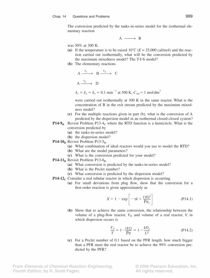
© 2006 Pearson Education, Inc.All rights reserved.
From Elements of Chemical Reaction Engineering,Fourth Edition, by H. Scott Fogler.
Chap. 14 Questions and Problems
999
The conversion predicted by the tanks-in-series model for the isothermal ele-mentary reaction
A B
was 50% at 300 K.
(a)
If the temperature is to be raised 10˚C (
E
= 25,000 cal/mol) and the reac-tion carried out isothermally, what will be the conversion predicted bythe maximum mixedness model? The T-I-S model?
(b)
The elementary reactions
were carried out isothermally at 300 K in the same reactor. What is theconcentration of B in the exit stream predicted by the maximum mixed-ness model?
(c)
For the multiple reactions given in part (b), what is the conversion of Apredicted by the dispersion model in an isothermal closed-closed system?
P14-9
B
Revisit Problem P13-4
C
where the RTD function is a hemicircle. What is theconversion predicted by
(a)
the tanks-in-series model?
(b)
the dispersion model?
P14-10
B
Revisit Problem P13-5
B
.
(a)
What combination of ideal reactors would you use to model the RTD?
(b)
What are the model parameters?
(c)
What is the conversion predicted for your model?
P14-11
B
Revisit Problem P13-6
B
.
(a)
What conversion is predicted by the tanks-in-series model?
(b)
What is the Peclet number?
(c)
What conversion is predicted by the dispersion model?
P14-12
C
Consider a real tubular reactor in which dispersion is occurring.
(a)
For small deviations from plug flow, show that the conversion for afirst-order reaction is given approximately as
X
�
1
�
exp (P14.1)
(b)
Show that to achieve the same conversion, the relationship between thevolume of a plug-flow reactor,
V
P
, and volume of a real reactor,
V,
inwhich dispersion occurs is
(P14.2)
(c)
For a Peclet number of 0.1 based on the PFR length, how much biggerthan a PFR must the real reactor be to achieve the 99% conversion pre-dicted by the PFR?
ææÆ
A ææÆ k
1 B ææÆ
k
2 C
A ææÆ k
3 D
k1 k2 k3 0.1 min 1� at 300 K, CA0 1 mol/dm3�� � �
tk�tk( )2
Per
-----------�
VP
V------ 1 kt( )
Pe---------� 1
kDe
U2---------�� �
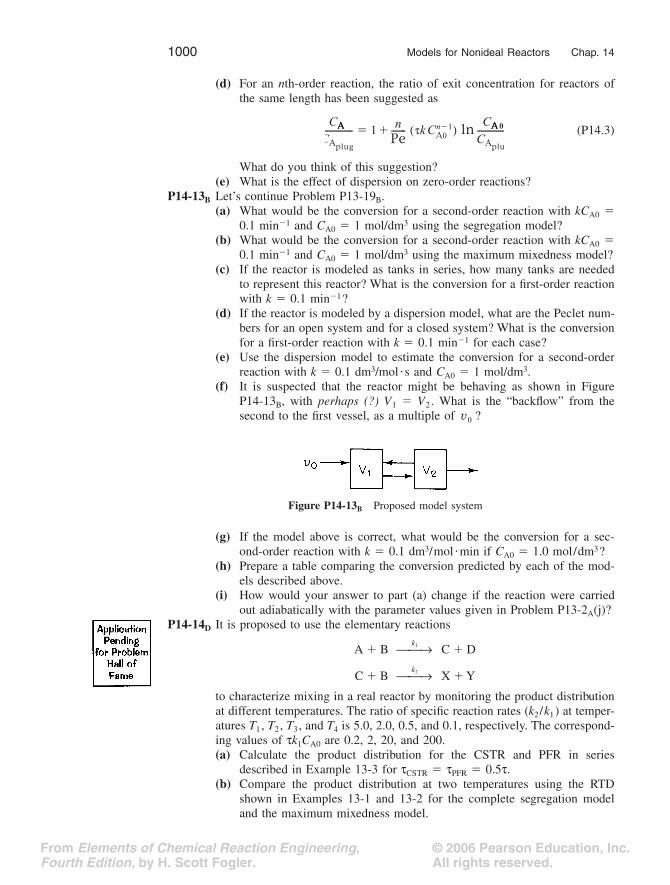
© 2006 Pearson Education, Inc.All rights reserved.
From Elements of Chemical Reaction Engineering,Fourth Edition, by H. Scott Fogler.
1000
Models for Nonideal Reactors Chap. 14
(d)
For an
n
th-order reaction, the ratio of exit concentration for reactors ofthe same length has been suggested as
(P14.3)
What do you think of this suggestion?
(e)
What is the effect of dispersion on zero-order reactions?
P14-13
B
Let’s continue Problem P13-19
B
.
(a)
What would be the conversion for a second-order reaction with
kC
A0
�
0.1 min
�
1
and
C
A0
�
1 mol/dm
3
using the segregation model?
(b)
What would be the conversion for a second-order reaction with
kC
A0
�
0.1 min
�
1
and
C
A0
�
1 mol/dm
3
using the maximum mixedness model?
(c) If the reactor is modeled as tanks in series, how many tanks are neededto represent this reactor? What is the conversion for a first-order reactionwith
k
�
0.1 min
�
1
?
(d)
If the reactor is modeled by a dispersion model, what are the Peclet num-bers for an open system and for a closed system? What is the conversionfor a first-order reaction with
k
�
0.1 min
�
1
for each case?
(e) Use the dispersion model to estimate the conversion for a second-orderreaction with k � 0.1 dm3/mol�s and CA0 � 1 mol/dm3.
(f) It is suspected that the reactor might be behaving as shown in FigureP14-13B, with perhaps (?) V1 � V2. What is the “backflow” from thesecond to the first vessel, as a multiple of ?
(g) If the model above is correct, what would be the conversion for a sec-ond-order reaction with k � 0.1 dm3/mol�min if CA0 � 1.0 mol/dm3?
(h) Prepare a table comparing the conversion predicted by each of the mod-els described above.
(i) How would your answer to part (a) change if the reaction were carriedout adiabatically with the parameter values given in Problem P13-2A(j)?
P14-14D It is proposed to use the elementary reactions
A � B C � D
C � B X � Y
to characterize mixing in a real reactor by monitoring the product distributionat different temperatures. The ratio of specific reaction rates (k2/k1) at temper-atures T1, T2, T3, and T4 is 5.0, 2.0, 0.5, and 0.1, respectively. The correspond-ing values of tk1CA0 are 0.2, 2, 20, and 200.(a) Calculate the product distribution for the CSTR and PFR in series
described in Example 13-3 for tCSTR � tPFR � 0.5t.(b) Compare the product distribution at two temperatures using the RTD
shown in Examples 13-1 and 13-2 for the complete segregation modeland the maximum mixedness model.
CAAAACAplug
-------------- 1 nPe------- t k C A
0
n
� 1 ( ) C AAAA
0 C
Aplu
-------------- ln ��
v0
Figure P14-13B Proposed model system
ææÆ k
1
ææÆ k
2

© 2006 Pearson Education, Inc.All rights reserved.
From Elements of Chemical Reaction Engineering,Fourth Edition, by H. Scott Fogler.
Chap. 14 Questions and Problems
1001
(c)
Explain how you could use the product distribution as a function of tem-perature (and perhaps flow rate) to characterize your reactor. For example,could you use the test reactions to determine whether the early mixingscheme or the late mixing scheme in Example 13-3 is more representativeof a real reactor? Recall that both schemes have the same RTD.
(d)
How should the reactions be carried out (i.e., at high or low tempera-tures) for the product distribution to best characterize the micromixing inthe reactor?
P14-15
B
A second-order reaction is to be carried out in a real reactor which gives thefollowing outlet concentration for a step input.
For 0
£
t
< 10 min then
C
T
= 10 (1
�
e
�
.1
t
)For 10 min
£
t
then
C
T
= 5
�
10 (1
�
e
�
.1
t
)
(a)
What model do you propose and what are your model parameters,
a
and
b
?
(b)
What conversion can be expected in the real reactor?
(c)
How would your model change and conversion change if your outlettracer concentration was
For
t
£
10 min, then
C
T
= 0 For
t
≥
10 min, then
C
T
= 5
�
10 (1
�
e
–0.2(t�10))
v0 = 1 dm3/min, k = 0.1 dm3/mol ◊ min, CA0 = 1.25 mol/dm3
P14-16B Suggest combinations of ideal reactors to model real reactors given in prob-lem P13-2A(b) for either E(q),E(t), F(q), F(t), or (1 – F(q)).
P14-17B Below are two COMSOL simulations for a laminar flow reactor with heateffects: Run 1 and Run 2. The figures below show the cross-section plot ofconcentration for species A at the middle of the reactor. Run 2 shows a min-imum on the cross-section plot. This minimum could be the result of (circleall that apply and explain your reasoning for each suggestion (a) through (e))(a) the thermal conductivity of reaction mixture decreases(b) overall heat transfer coefficient increases(c) overall heat transfer coefficient decreases(d) the coolant flow rate increases(e) the coolant flow rate decreasesHint: Explore “Nonisothermal Reactor II” on the COMSOL CD-ROM.
Figure P14-17B COMSOL screen shots
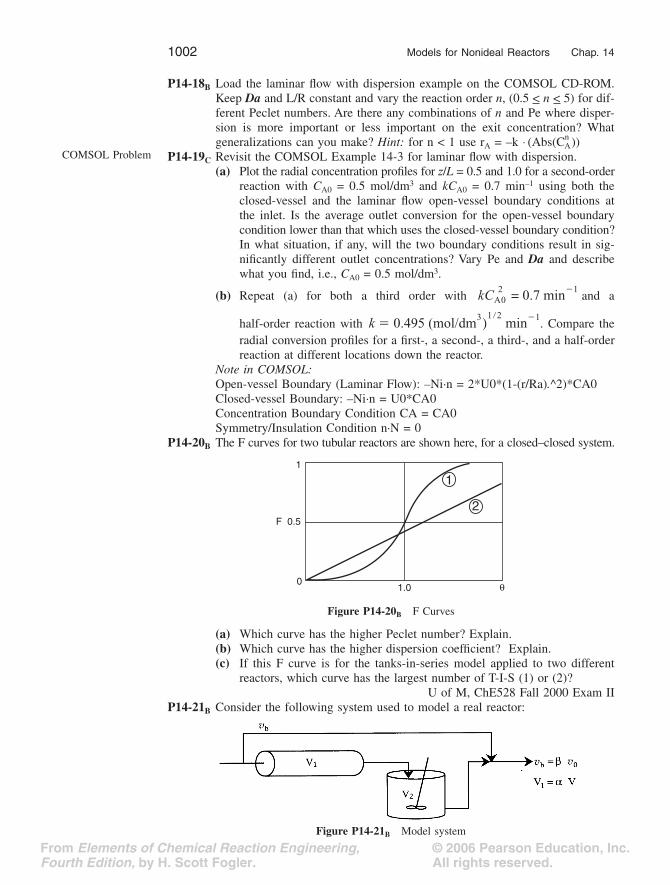
© 2006 Pearson Education, Inc.All rights reserved.
From Elements of Chemical Reaction Engineering,Fourth Edition, by H. Scott Fogler.
1002 Models for Nonideal Reactors Chap. 14
P14-18B Load the laminar flow with dispersion example on the COMSOL CD-ROM.Keep Da and L/R constant and vary the reaction order n, (0.5 < n < 5) for dif-ferent Peclet numbers. Are there any combinations of n and Pe where disper-sion is more important or less important on the exit concentration? Whatgeneralizations can you make? Hint: for n < 1 use rA = –k ◊ (Abs(Cn
A))P14-19C Revisit the COMSOL Example 14-3 for laminar flow with dispersion.
(a) Plot the radial concentration profiles for z/L = 0.5 and 1.0 for a second-orderreaction with CA0 = 0.5 mol/dm3 and kCA0 = 0.7 min–1 using both theclosed-vessel and the laminar flow open-vessel boundary conditions atthe inlet. Is the average outlet conversion for the open-vessel boundarycondition lower than that which uses the closed-vessel boundary condition?In what situation, if any, will the two boundary conditions result in sig-nificantly different outlet concentrations? Vary Pe and Da and describewhat you find, i.e., CA0 = 0.5 mol/dm3.
(b) Repeat (a) for both a third order with and a
half-order reaction with . Compare theradial conversion profiles for a first-, a second-, a third-, and a half-orderreaction at different locations down the reactor.
Note in COMSOL:Open-vessel Boundary (Laminar Flow): –Ni·n = 2*U0*(1-(r/Ra).^2)*CA0Closed-vessel Boundary: –Ni·n = U0*CA0Concentration Boundary Condition CA = CA0Symmetry/Insulation Condition n·N = 0
P14-20B The F curves for two tubular reactors are shown here, for a closed–closed system.
(a) Which curve has the higher Peclet number? Explain.(b) Which curve has the higher dispersion coefficient? Explain.(c) If this F curve is for the tanks-in-series model applied to two different
reactors, which curve has the largest number of T-I-S (1) or (2)?U of M, ChE528 Fall 2000 Exam II
P14-21B Consider the following system used to model a real reactor:
COMSOL Problem
kCA02 0.7 min 1�=
k 0.495 (mol/dm3)1 2�
min 1��
1
F 0.5
01.0 θ
1
2
Figure P14-20B F Curves
Figure P14-21B Model system
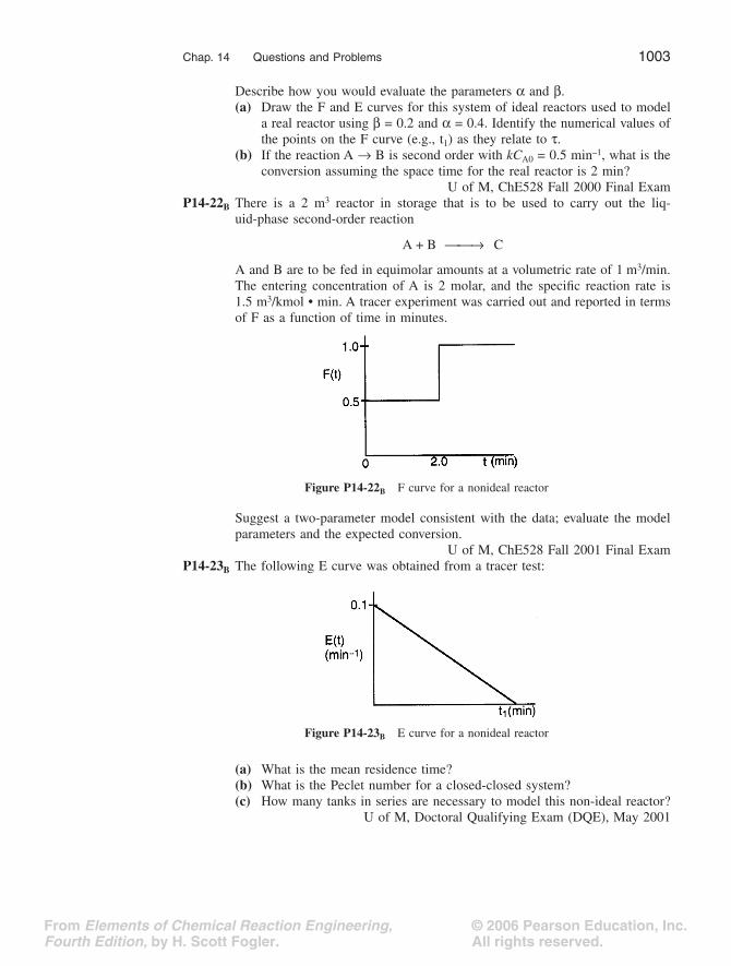
© 2006 Pearson Education, Inc.All rights reserved.
From Elements of Chemical Reaction Engineering,Fourth Edition, by H. Scott Fogler.
Chap. 14 Questions and Problems 1003
Describe how you would evaluate the parameters a and b.(a) Draw the F and E curves for this system of ideal reactors used to model
a real reactor using b = 0.2 and a = 0.4. Identify the numerical values ofthe points on the F curve (e.g., t1) as they relate to t.
(b) If the reaction A Æ B is second order with kCA0 = 0.5 min–1, what is theconversion assuming the space time for the real reactor is 2 min?
U of M, ChE528 Fall 2000 Final ExamP14-22B There is a 2 m3 reactor in storage that is to be used to carry out the liq-
uid-phase second-order reaction
A + B C
A and B are to be fed in equimolar amounts at a volumetric rate of 1 m3/min.The entering concentration of A is 2 molar, and the specific reaction rate is1.5 m3/kmol • min. A tracer experiment was carried out and reported in termsof F as a function of time in minutes.
Suggest a two-parameter model consistent with the data; evaluate the modelparameters and the expected conversion.
U of M, ChE528 Fall 2001 Final ExamP14-23B The following E curve was obtained from a tracer test:
(a) What is the mean residence time?(b) What is the Peclet number for a closed-closed system?(c) How many tanks in series are necessary to model this non-ideal reactor?
U of M, Doctoral Qualifying Exam (DQE), May 2001
ææÆ
Figure P14-22B F curve for a nonideal reactor
Figure P14-23B E curve for a nonideal reactor

© 2006 Pearson Education, Inc.All rights reserved.
From Elements of Chemical Reaction Engineering,Fourth Edition, by H. Scott Fogler.
1004
Models for Nonideal Reactors Chap. 14
P14-24
B
The A first-order reaction is to be carried out in the reactor with
k
= 0.1 min
–1
.
Fill in the following table with the conversion predicted by each type ofmodel/reactor.
P14-25
B
The following outlet concentration trajectory was obtained from a step inputto a nonideal reactor. The entering concentration was 10 millimolar of tracer.
Suggest a model using a collection of ideal reactors to model the nonidealreactor.
U of M, Doctoral Qualifying Exam (DQE), May 2001
∑
Additional Homework Problems
CDP14-A
C
A real reactor is modeled as
a combination of ideal PFRs andCSTRs.
[2nd Ed. P14-5]
CDP14-B
B
A real batch reactor is modeled as a combination of two ideal reactors.[2nd Ed. P14-13]
CDP14-C
C
Develop a model for a real reactor for RTD obtained from a stepinput. [2nd Ed. P14-10]
CDP14-D
B
Calculate
D
a
and
X
from sloppy tracer data. [2nd Ed. P14-6
A
]
CDP14-E
B
Use RTD data from Oak Ridge National Laboratory to calculate theconversion from the tanks-in-series and the dispersion models. [2ndEd. P14-7
B
]
CDP14-F
B
RTD data from a slurry reactor. [3rd Ed. P14-8]
Ideal PFR Ideal CSTR
Ideallaminar
flow reactor SegregationMaximum mixedness Dispersion
Tanks in series
2010t (min)
E(t)(min–1)
Figure P14-25B C curve for a nonideal reactor
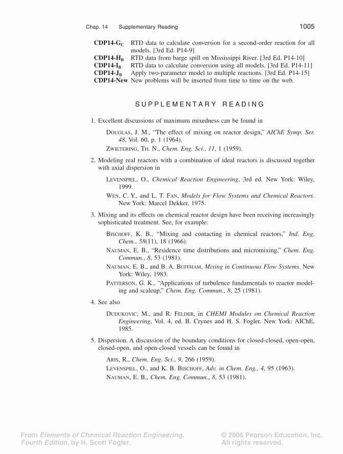
© 2006 Pearson Education, Inc.All rights reserved.
From Elements of Chemical Reaction Engineering,Fourth Edition, by H. Scott Fogler.
Chap. 14 Supplementary Reading
1005
CDP14-G
C
RTD data to calculate conversion for a second-order reaction for allmodels. [3rd Ed. P14-9]
CDP14-H
B
RTD data from barge spill on Mississippi River. [3rd Ed. P14-10]
CDP14-I
B
RTD data to calculate conversion using all models. [3rd Ed. P14-11]CDP14-JB Apply two-parameter model to multiple reactions. [3rd Ed. P14-15]CDP14-New New problems will be inserted from time to time on the web.
S U P P L E M E N T A R Y R E A D I N G
1. Excellent discussions of maximum mixedness can be found in
DOUGLAS, J. M., “The effect of mixing on reactor design,” AIChE Symp. Ser.48, Vol. 60, p. 1 (1964).
ZWIETERING, TH. N., Chem. Eng. Sci., 11, 1 (1959).
2. Modeling real reactors with a combination of ideal reactors is discussed togetherwith axial dispersion in
LEVENSPIEL, O., Chemical Reaction Engineering, 3rd ed. New York: Wiley,1999.
WEN, C. Y., and L. T. FAN, Models for Flow Systems and Chemical Reactors.New York: Marcel Dekker, 1975.
3. Mixing and its effects on chemical reactor design have been receiving increasinglysophisticated treatment. See, for example:
BISCHOFF, K. B., “Mixing and contacting in chemical reactors,” Ind. Eng.Chem., 58(11), 18 (1966).
NAUMAN, E. B., “Residence time distributions and micromixing,” Chem. Eng.Commun., 8, 53 (1981).
NAUMAN, E. B., and B. A. BUFFHAM, Mixing in Continuous Flow Systems. NewYork: Wiley, 1983.
PATTERSON, G. K., “Applications of turbulence fundamentals to reactor model-ing and scaleup,” Chem. Eng. Commun., 8, 25 (1981).
4. See also
DUDUKOVIC, M., and R. FELDER, in CHEMI Modules on Chemical ReactionEngineering, Vol. 4, ed. B. Crynes and H. S. Fogler. New York: AIChE,1985.
5. Dispersion. A discussion of the boundary conditions for closed-closed, open-open,closed-open, and open-closed vessels can be found in
ARIS, R., Chem. Eng. Sci., 9, 266 (1959).LEVENSPIEL, O., and K. B. BISCHOFF, Adv. in Chem. Eng., 4, 95 (1963).NAUMAN, E. B., Chem. Eng. Commun., 8, 53 (1981).

© 2006 Pearson Education, Inc.All rights reserved.
From Elements of Chemical Reaction Engineering,Fourth Edition, by H. Scott Fogler.
1006 Models for Nonideal Reactors Chap. 14
This is not the end.It is not even the beginning of the end.But it is, perhaps, the end of the beginning.
Winston ChurchillNovember 10, 1942