copyright by john timothy cullinane 2005
TRANSCRIPT

Copyright
by
John Timothy Cullinane
2005
The Dissertation Committee for John Timothy Cullinane certifies that this is the approved version of the following dissertation:
Thermodynamics and Kinetics of Aqueous Piperazine with Potassium
Carbonate for Carbon Dioxide Absorption
Committee:
_______________________ Gary Rochelle, Supervisor
_______________________ John G. Ekerdt
_______________________ Benny D. Freeman
_______________________ Craig Schubert
_______________________ Frank Seibert
Thermodynamics and Kinetics of Aqueous Piperazine with Potassium
Carbonate for Carbon Dioxide Absorption
by
John Timothy Cullinane, B.S.; M.S.
Dissertation
Presented to the Faculty of the Graduate School of
the University of Texas at Austin
in Partial Fulfillment
of the Requirements
for the Degree of
Doctor of Philosophy
The University of Texas at Austin
May, 2005

To My Family

v
Acknowledgments
I would like to acknowledge Dr. Gary Rochelle for his support and contribution
to this work. My work has exposed me to a wide variety of topics and sciences and I
thank him for his direction throughout the research project. Dr. Rochelle has also been
very generous in providing opportunities to expand my experience outside of research,
including two international conferences and numerous national meetings. Dr. Rochelle
has been a positive influence on my professional development and I appreciate his
patience and teaching.
I thank the various financial contributors who have made this project possible.
The Texas Advanced Technology Program, Separations Research Program, and various
industrial sponsors have each provided me necessary means of support.
Throughout my academic career at UT, I have relied in large part on the help of
Jody Lester. She has been a great help to me. I am very thankful to Jody for making
my stay here easier.
I have had the pleasure of interacting professionally and personally with a
number of students in Dr. Rochelle�s research group, including Dyron Hamlin, Ross
Dugas, Eric Chen, Tunde Oyenekan, and Akin Alawode. Thanks to Dan Ellenberger
for his hard work on the solid solubility studies. I would also like to thank Stefano
Freguia, Marcus Hilliard, and Dr. Mohammed Al-Juaied for their help and friendship.
Dr. Norman Yeh was one of the few �senior� graduate students here during the early
part of my work. His guidance and friendship is also very much appreciated. I have
vi
also worked with several undergraduate students during my work here. Thanks to Dan
Ellenberger for his help on the density, viscosity, and solid solubility work.
I would like to extend special thanks to George Goff. I have thoroughly enjoyed
the past four years of sharing a lab and many of the same experiences, hardships, and
character-building experiences. George has been extremely helpful in my development
as a researcher; I always learned from our discussions of research ideas. We�ve also
shared plenty of memorable times outside of work. George has been a good co-worker
and a good friend and I thank him for that.
During my graduate career, I have had many opportunities. In particular, the
chance to interact with industrial sponsors has greatly enhanced my learning. I would
like to thank Dr. Craig Schubert of The Dow Chemical Company and Dr. Jim
Critchfield of Huntsman Chemical for their time and interest in my research and
professional development.
I have also had the pleasure of take classes and learning from some excellent
faculty members including Professors Bill Koros, Venkat Ganesan, and Buddy Mullins.
Professor Bruce Eldridge was also a valuable part of my learning, not only from a
teaching standpoint, but as part of the SRP program. I thank Professor Del Ottmers for
the opportunity to TA under his tutelage. Professor Ben Shoulders from the UT
Department of Chemistry was a tremendous help with the NMR measurements.
Thanks to my family. My mother and father have been tremendous influences
on me and have been wonderful role models. My father, being an engineer himself, has
always been available for my questions and taken an interest in my career. My

vii
mother�s constant encouragement has helped support me throughout my academic
career. I will always be grateful to them for the opportunities they have provided to me.
Finally, I would like to thank my wife, Christa. She has been very
understanding with the time I have devoted to this work and has been a constant source
of encouragement. Her contributions to our home have made my time at work easier
and her companionship has made me a better person.

viii
Thermodynamics and Kinetics of Aqueous Piperazine with Potassium
Carbonate for Carbon Dioxide Absorption
Publication No. ________
John Timothy Cullinane, Ph.D.
The University of Texas at Austin, 2005
Supervisor: Gary T. Rochelle
This work proposes an innovative blend of potassium carbonate (K2CO3) and
piperazine (PZ) as a solvent for CO2 removal from combustion flue gas in an
absorber/stripper. The equilibrium partial pressure and the rate of absorption of CO2
were measured in a wetted-wall column in 0.0 to 6.2 m K+ and 0.6 to 3.6 m PZ at 25 to
110oC. The equilibrium speciation of the solution was determined by 1H NMR under
similar conditions. A rigorous thermodynamic model, based on electrolyte non-random
two-liquid (ENRTL) theory, was developed to represent equilibrium behavior. A rate
model was developed to describe the absorption rate by integration of eddy diffusivity
theory with complex kinetics. Both models were used to explain behavior in terms of
equilibrium constants, activity coefficients, and rate constants.
The addition of potassium to the amine increases the concentration of CO32-
/HCO3- in solution. The buffer reduces protonation of the amine, but increases the

ix
amount of carbamate species, yielding a maximum reactive species concentration at a
K+:PZ ratio of 2:1. The carbamate stability of piperazine carbamate and dicarbamate
resembles that of primary amines and has approximately equal values for the heats of
reaction, ∆Hrxn (18.3 and 16.5 kJ/mol). The heat of CO2 absorption is lowered by K+
from -75 to -40 kJ/mol. The capacity increases as total solute concentration increases,
comparing favorably with 5 M monoethanolamine (MEA).
The rate approaches second-order behavior with PZ and is highly dependent on
other strong bases. In 1 M PZ, the overall rate constant is 102,000 s-1, 20 times higher
than in MEA. The activation energy is 35 kJ/kmol. In K+/PZ, the most significant
reactions are PZ and piperazine carbamate with CO2 catalyzed by carbonate. Neutral
salts in aqueous PZ increase the apparent rate constant, by a factor of 8 at 3 M ionic
strength. The absorption rate in 5 m K+/2.5 m PZ is 3 times faster than 30 wt% MEA.
A pseudo-first order approximation represents the absorption rate under limited
conditions. At high loadings, the reaction approaches instantaneous behavior. Under
industrial conditions, gas film resistance may account for >80% of the total mass
transfer resistance at low loadings.
x
Contents
List of Tables ................................................................................................................. xiv
List of Figures..............................................................................................................xviii
Chapter 1: Introduction..................................................................................................... 1
1.1. Emission and Remediation of Carbon Dioxide ..................................................... 1 1.1.1. Sources of Carbon Dioxide............................................................................. 2 1.1.2. Carbon Dioxide Capture ................................................................................. 5 1.1.3. Sinks and Sequestration of Carbon Dioxide ................................................... 6
1.2. Carbon Dioxide Capture by Absorption/Stripping................................................ 8 1.2.1. Technology Description.................................................................................. 8 1.2.2. Factors in Cost .............................................................................................. 10 1.2.3. Solvents......................................................................................................... 12
1.3. Potassium Carbonate/Piperazine for Carbon Dioxide Capture ........................... 14 1.3.1. Solvent Description ...................................................................................... 14 1.3.2. Research Needs............................................................................................. 15 1.3.3. Previous Work .............................................................................................. 16 1.3.4. Objectives and Scope.................................................................................... 17
Chapter 2: Literature Review.......................................................................................... 21
2.1. Mass Transfer with Fast Chemical Reaction....................................................... 21 2.1.1. Mass Transfer Theory................................................................................... 21 2.1.2. Mass Transfer Models .................................................................................. 25 2.1.3. Reversible Reactions .................................................................................... 26 2.1.4. Pseudo-First Order Reaction......................................................................... 27 2.1.5. Instantaneous Reactions................................................................................ 28
2.2. Solvents for CO2 Absorption............................................................................... 30 2.2.1. Potassium Carbonate..................................................................................... 30 2.2.2. Primary and Secondary Amines ................................................................... 32 2.2.3. Tertiary Amines ............................................................................................ 35 2.2.4. Hindered Amines .......................................................................................... 36 2.2.5. Piperazine...................................................................................................... 38 2.2.6. Amine-Promoted Potassium Carbonate........................................................ 38
2.3. Contributions to Reaction Kinetics...................................................................... 43
xi
2.3.1. Acid and Base Catalysis ............................................................................... 43 2.3.2. Neutral Salt Effects....................................................................................... 46
Chapter 3: Experimental Methods .................................................................................. 51
3.1. Wetted-Wall Column........................................................................................... 51 3.1.1. Equipment Description ................................................................................. 52 3.1.2. Gas Analysis ................................................................................................. 55 3.1.3. Liquid Analysis............................................................................................. 55 3.1.4. Physical Mass Transfer Coefficients ............................................................ 56 3.1.5. Interpretation of Experimental Measurements ............................................. 60
3.2. Nuclear Magnetic Resonance Spectroscopy........................................................ 62
3.3. Solid Solubility .................................................................................................... 64
3.4. Physical Properties .............................................................................................. 66 3.4.1. Density .......................................................................................................... 66 3.4.2. Viscosity ....................................................................................................... 67 3.4.3. Physical Solubility ........................................................................................ 70 3.4.4. Diffusion Coefficient .................................................................................... 73
3.5. Chemicals and Materials ..................................................................................... 76
Chapter 4: Thermodynamic and Rate Models ................................................................ 77
4.1. Thermodynamics Model...................................................................................... 78 4.1.1. Introduction................................................................................................... 78 4.1.2. Chemical Equilibrium and Excess Gibbs Energy......................................... 79 4.1.3. Electrolyte NRTL Model .............................................................................. 81 4.1.4. Thermodynamic Model Default Settings...................................................... 88 4.1.5. Vapor-Liquid Equilibrium ............................................................................ 89 4.1.6. Reference States............................................................................................ 91 4.1.7. Solution Method (Non-Stoichiometric Method) .......................................... 92
4.2. Kinetic/Rate Model.............................................................................................. 94 4.2.1. Introduction................................................................................................... 94 4.2.2. Modeling Mass Transfer with Chemical Reaction ....................................... 95 4.2.3. Rate Expressions........................................................................................... 99 4.2.4. Solution Method ......................................................................................... 103
4.3. Non-Linear Regression Model .......................................................................... 104 4.3.1. Description of GREG ................................................................................. 104 4.3.2. Interface with the Thermodynamic and Rate Models................................. 104
xii
4.3.3. Results and Statistics from GREG.............................................................. 106
Chapter 5: Thermodynamics of Potassium Carbonate, Piperazine, and Carbon Dioxide Mixtures...................................................................................................... 108
5.1. Model Description ............................................................................................. 109
5.2. Physical Solubility............................................................................................. 112
5.3. Aqueous Potassium Carbonate/Bicarbonate...................................................... 117
5.4. Aqueous Piperazine ........................................................................................... 121 5.4.1. Infinite Dilution Activity Coefficient and Solution Enthalpy .................... 121 5.4.2. Dissociation of Piperazine .......................................................................... 124 5.4.3. Regression of Parameters for Aqueous Piperazine..................................... 126 5.4.4. Liquid Phase Equilibrium ........................................................................... 129 5.4.5. Vapor-Liquid Equilibrium .......................................................................... 135
5.5. Aqueous Potassium/Piperazine Mixtures .......................................................... 138 5.5.1. Liquid Phase Equilibrium ........................................................................... 138 5.5.2. Vapor-Liquid Equilibrium .......................................................................... 148
5.6. Capacity ............................................................................................................. 156
5.7. Heat of Absorption ............................................................................................ 159
5.8. Stoichiometry and Enthalpy .............................................................................. 162
5.9. Solid Solubility .................................................................................................. 167
5.10. Conclusions ..................................................................................................... 172
Chapter 6: Rate and Kinetics of Potassium Carbonate, Piperazine and Carbon Dioxide Mixtures...................................................................................................... 175
6.1. Model Description ............................................................................................. 176
6.2. Aqueous Piperazine ........................................................................................... 177 6.2.1. Rate Constants ............................................................................................ 177 6.2.2. Absorption Rate of Carbon Dioxide ........................................................... 182 6.2.3. Neutral Salt Effects..................................................................................... 183
6.3. Aqueous Potassium Carbonate/Piperazine ........................................................ 187 6.3.1. Parameter Regression and Correlation ....................................................... 188 6.3.2. Absorption Rate of Carbon Dioxide ........................................................... 194 6.3.3. Approximations .......................................................................................... 200 6.3.4. Applications ................................................................................................ 206
6.4. Conclusions ....................................................................................................... 209
xiii
Chapter 7: Conclusions and Recommendations ........................................................... 212
7.1. Summary............................................................................................................ 212
7.2. Conclusions ....................................................................................................... 213 7.2.1. Thermodynamics ........................................................................................ 213 7.2.2. Kinetics ....................................................................................................... 216 7.2.3. Potassium Carbonate/Piperazine as a Unique Solvent for CO2 Capture .... 218
7.3. Recommendations for Future Studies................................................................ 220 7.3.1. Thermodynamics ........................................................................................ 220 7.3.2. Kinetics ....................................................................................................... 221 7.3.3. General........................................................................................................ 223
Appendix A: Density and Viscosity Results ................................................................ 225
A.1. Density Results ................................................................................................. 225
A.2. Viscosity Results .............................................................................................. 227
Appendix B: Detailed 1H NMR Data ........................................................................... 229
B.1. 1H NMR Data .................................................................................................... 229
B.2. Samples Not Used............................................................................................. 247
B.3. Example Spectra ............................................................................................... 249
Appendix C: Detailed Wetted-Wall Column Data ....................................................... 252
Appendix D: Tabulated Model Predictions .................................................................. 263
D.1. PCO2* and Speciation Predictions ..................................................................... 263
D.2. PCO2* and Normalized Flux .............................................................................. 272
D.3. Concentration Profiles ...................................................................................... 278
Bibliography ................................................................................................................. 282
Vita ............................................................................................................................... 296

xiv
List of Tables Table 1.1. Annual CO2 Emissions in the United States in Tg CO2 Eq............................ 2 Table 1.2. Process Conditions in Absorber/Stripper Applications to CO2
Capture................................................................................................................ 10 Table 1.3. Common Amines in Gas Treating (Kohl and Riesenfeld, 1985) ................. 13 Table 1.4. Summary of Previous Work on Piperazine .................................................. 16 Table 2.1. Selected Studies of Amine-Promoted K2CO3............................................... 40 Table 3.1. Coefficients for Empirical Viscosity Model................................................. 70 Table 4.1. Dielectric Constants of Molecular Species in the ENRTL Model ............... 83 Table 5.1. Defined Equilibrium Constants (Mole Fraction-Based) in the ENRTL
Model................................................................................................................ 110 Table 5.2. Summary of Data and Sources for the Regression of Parameters in
the ENRTL Model ............................................................................................ 111 Table 5.3. Regressed Binary Interaction Parameters for the ENRTL Model .............. 112 Table 5.4. Physical Solubility of CO2 in Aqueous PZ................................................. 114 Table 5.5. Physical Solubility of CO2 in Aqueous K2CO3/KHCO3 ............................ 115 Table 5.6. Physical Solubility of CO2 in Aqueous K+/PZ Mixtures............................ 116 Table 5.7. Enthalpies (kJ/mol) of Phase Change for Piperazine ................................. 124 Table 5.8. Enthalpy of Solution (kJ/mol) for PZ at Infinite Dilution in Water ........... 124 Table 5.9. Summary of pKa (Molarity-based, Infinite Dilution in Water)
Investigations of Aqueous PZ........................................................................... 125 Table 5.10. Regressed Equilibrium Constants in Electrolyte NRTL Model,
Mole Fraction-Based ........................................................................................ 127 Table 5.11. Correlation Matrix for the Simultaneous Regression of Equilibrium
Constants and τ Parameters in PZ/H2O/CO2 .................................................... 128 Table 5.12. Equilibrium Constants and Temperature Dependences at 40oC
(Mole Fraction-Based, Infinite Dilution in Water) from Four Studies............. 128 Table 5.13. Piperazine Speciation in K+/PZ as Determined from 1H NMR................ 138 Table 5.14. Comparison of Concentration-based (Molarity) Carbamate Stability
Constants at 40oC.............................................................................................. 148 Table 5.15. Vapor Pressure of CO2 over K+/PZ Mixtures at 40 to 110oC................... 149 Table 5.16. Calculated Heats of Formation at 25oC .................................................... 165 Table 5.17. Phase Behavior in K2CO3/PZ at 25 and 40oC........................................... 168 Table 5.18. Phase Behavior in KHCO3/PZ at 25 and 40oC ......................................... 169
xv
Table 6.1. Regressed Constants for Modeling CO2 Absorption into K+/PZ ............... 176 Table 6.2. Absorption rate of CO2 into Aqueous PZ................................................... 178 Table 6.3. Overall Rate Constants for 1.0 M Amines at 25oC..................................... 180 Table 6.4. Absorption rate of CO2 into 0.6 m PZ at High Ionic Strength ................... 185 Table 6.5. Termolecular Rate Constants (kAm-base (m6/kmol2-s)) for Four
Secondary Amines Interpreted from Previous Work at 25oC........................... 191 Table 6.6. Concentration (kmol/m3) Across the Liquid Boundary Layer in 5.0 m
K+/2.5 m PZ, klo = 1.0x10⁻⁴ m/s........................................................................ 204
Table A.1. Density of K2CO3 and KHCO3 at 25 and 40oC ......................................... 225 Table A.2. Density of Aqueous PZ at 25 and 40oC at Zero Loading .......................... 226 Table A.3. Density of K+/PZ Mixtures at 25 and 40oC ............................................... 226 Table A.4. Viscosity of Aqueous PZ at 25 to 70oC ..................................................... 227 Table A.5. Viscosity of K+/PZ Mixtures at 25 to 70oC ............................................... 228 Table B.1. 3.60 m K+/0.60 m PZ, α = 0.357 ............................................................... 229
Table B.2. 3.59 m K+/0.60 m PZ, α = 0.429 ............................................................... 230 Table B.3. 3.60 m K+/0.60 m PZ, α = 0.441 ............................................................... 231 Table B.4. 3.60 m K+/0.61 m PZ, α = 0.486 ............................................................... 232
Table B.5. 3.59 m K+/0.61 m PZ, α = 0.515 ............................................................... 233 Table B.6. 3.56 m K+/0.61 m PZ, α = 0.554 ............................................................... 234
Table B.7. 3.58 m K+/0.60 m PZ, α = 0.601 ............................................................... 235 Table B.8. 3.59 m K+/0.61 m PZ, α = 0.630 ............................................................... 236 Table B.9. 3.59 m K+/1.81 m PZ, α = 0.433 ............................................................... 237
Table B.10. 3.44 m K+/1.85 m PZ, α = 0.618 ............................................................. 238 Table B.11. 3.46 m K+/1.86 m PZ, α = 0.694 ............................................................. 238 Table B.12. 3.60 m K+/3.58 m PZ, α = 0.376 ............................................................. 239
Table B.13. 3.57 m K+/3.58 m PZ, α = 0.499 ............................................................. 239 Table B.14. 3.59 m K+/3.61 m PZ, α = 0.600 ............................................................. 240 Table B.15. 3.60 m K+/3.60 m PZ, α = 0.646 ............................................................. 240
Table B.16. 5.00 m K+/2.50 m PZ, α = 0.433 ............................................................. 241 Table B.17. 4.99 m K+/2.51 m PZ, α = 0.467 ............................................................. 242 Table B.18. 4.98 m K+/2.50 m PZ, α = 0.534 ............................................................. 243
Table B.19. 4.98 m K+/2.50 m PZ, α = 0.600 ............................................................. 244

xvi
Table B.20. 4.64 m K+/2.50 m PZ, α = 0.650 ............................................................. 244 Table B.21. 6.18 m K+/1.23 m PZ, α = 0.570 ............................................................. 245
Table B.22. 6.20 m K+/1.81 m PZ, α = 0.527 ............................................................. 246 Table B.23. 6.20 m K+/1.81 m PZ, α = 0.667 ............................................................. 246 Table B.24. 3.56 m K+/0.61 m PZ, α = 0.554, 100% D2O.......................................... 247
Table B.25. 3.33 m K/0.57 m PZ, α = 0.699............................................................... 247 Table B.26. 5.72 m K+/0.56 m PZ, α = 0.526 ............................................................. 248 Table B.27. 5.83 m K+/0.57 m PZ, α = 0.697 ............................................................. 248 Table C.1. Experimental Results for Wetted-Wall Column........................................ 253 Table D.1. Speciation in 1.8 m PZ at 40oC.................................................................. 264 Table D.2. Speciation in 1.8 m PZ at 60oC.................................................................. 264 Table D.3. Speciation in 1.8 m PZ at 80oC.................................................................. 265 Table D.4. Speciation in 1.8 m PZ at 110oC................................................................ 265 Table D.5. Speciation in 3.6 m K+/0.6 m PZ at 40oC .................................................. 266 Table D.6. Speciation in 3.6 m K+/0.6 m PZ at 60oC .................................................. 266 Table D.7. Speciation in 3.6 m K+/0.6 m PZ at 80oC .................................................. 267 Table D.8. Speciation in 3.6 m K+/0.6 m PZ at 110oC ................................................ 267 Table D.9. Speciation in 3.6 m K+/1.8 m PZ at 40oC .................................................. 268 Table D.10. Speciation in 3.6 m K+/1.8 m PZ at 60oC ................................................ 268 Table D.11. Speciation in 3.6 m K+/1.8 m PZ at 80oC ................................................ 269 Table D.12. Speciation in 3.6 m K+/1.8 m PZ at 110oC .............................................. 269 Table D.13. Speciation in 5.0 m K+/2.5 m PZ at 40oC ................................................ 270 Table D.14. Speciation in 5.0 m K+/2.5 m PZ at 60oC ................................................ 270 Table D.15. Speciation in 5.0 m K+/2.5 m PZ at 80oC ................................................ 271 Table D.16. Speciation in 5.0 m K+/2.5 m PZ at 110oC .............................................. 271 Table D.17. Partial Pressure and Rate Predictions in Aqueous PZ at 40oC ................ 272 Table D.18. Partial Pressure and Rate Predictions in Aqueous PZ at 60oC ................ 273 Table D.19. Partial Pressure and Rate Predictions in Aqueous PZ at 80oC ................ 273 Table D.20. Partial Pressure and Rate Predictions in Aqueous PZ at 100oC .............. 274 Table D.21. Partial Pressure and Rate Predictions in Aqueous PZ at 120oC .............. 274 Table D.22. Partial Pressure and Rate Predictions in K+/PZ at 40oC .......................... 275 Table D.23. Partial Pressure and Rate Predictions in K+/PZ at 60oC .......................... 275
xvii
Table D.24. Partial Pressure and Rate Predictions in K+/PZ at 80oC .......................... 275 Table D.25. Partial Pressure and Rate Predictions in K+/PZ at 100oC ........................ 276 Table D.26. Partial Pressure and Rate Predictions in K+/PZ at 120oC ........................ 276 Table D.27. Partial Pressure and Rate Predictions in K+/PZ at 40oC .......................... 276 Table D.28. Partial Pressure and Rate Predictions in K+/PZ at 60oC .......................... 277 Table D.29. Partial Pressure and Rate Predictions in K+/PZ at 80oC .......................... 277 Table D.30. Partial Pressure and Rate Predictions in K+/PZ at 100oC ........................ 277 Table D.31. Partial Pressure and Rate Predictions in K+/PZ at 120oC ........................ 278 Table D.32. Concentration Profile in 1.8 m PZ, 60oC................................................. 279 Table D.33. Concentration Profile in 3.6 m K+/0.6 m PZ, 60oC ................................. 280 Table D.34. Concentration Profile in 5.0 m K+/2.5 m PZ, 60oC ................................. 281
xviii
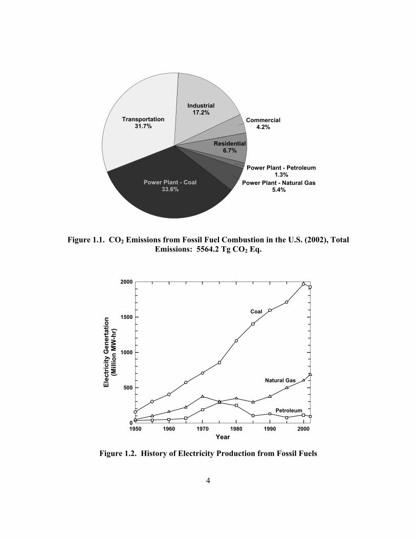
List of Figures Figure 1.1. CO2 Emissions from Fossil Fuel Combustion in the U.S. (2002),
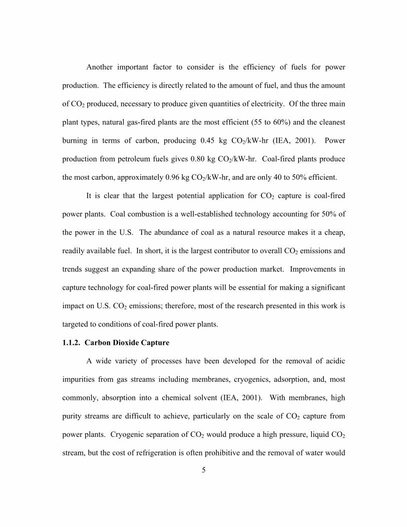
Total Emissions: 5564.2 Tg CO2 Eq.................................................................... 4 Figure 1.2. History of Electricity Production from Fossil Fuels ..................................... 4 Figure 1.3. Absorber/Stripper Process Flowsheet ........................................................... 9 Figure 1.4. Structures of Piperazine in the Presence of CO2 ......................................... 14 Figure 2.1. Physical Mass Transfer of CO2 into a Bulk Liquid..................................... 23 Figure 2.2. Mass Transfer of CO2 into a Bulk Liquid with Fast Chemical
Reaction .............................................................................................................. 24 Figure 3.1. Diagram of the Wetted-Wall Column Construction ................................... 52 Figure 3.2. Flowsheet of the Wetted-Wall Column Experiment ................................... 54 Figure 3.3. Gas Film Resistance as a Function of Gas Flowrate at 60oC with N2
Saturated to Water .............................................................................................. 58 Figure 3.4. Graphical Representation of Determining PCO2* and KG for 3.6 m
K+/0.6 m PZ at 40oC and Loading = 0.693 mol CO2/(mol K+ + mol PZ) .......... 61 Figure 3.5. Proton NMR Spectrum of 3.6 m K+/0.6 m PZ, Loading = 0.630 mol
CO2/(mol K+ + mol PZ), 27oC............................................................................ 63 Figure 3.6. Proton NMR Spectrum of 3.6 m K+/0.6 m PZ, Loading = 0.630 mol
CO2/(mol K+ + mol PZ), 60oC............................................................................ 64 Figure 3.7. Cannon-Fenske Viscometer ........................................................................ 69 Figure 3.8. Apparatus for Physical Solubility Measurements ....................................... 72 Figure 4.1. Distribution of Molecules as Cells in the Electrolyte NRTL Theory ......... 86 Figure 4.2. Transfer of Data during a Regression with GREG ................................... 105 Figure 5.1. Physical Solubility of CO2 in Aqueous PZ ............................................... 114 Figure 5.2. Physical Solubility of CO2 in K2CO3/KHCO3 at 25oC ............................. 115 Figure 5.3. Physical Solubility of CO2 in K+/PZ at 25oC ............................................ 116 Figure 5.4. Osmotic Coefficient of Water in Aqueous K2CO3 at 25oC....................... 118 Figure 5.5. PCO2
* in 20 wt% K2CO3, Points: Tosh et al. (1959), Lines: ENRTL ...... 120
Figure 5.6. PCO2* in 40 wt% K2CO3, Points: Tosh et al. (1959), Lines: ENRTL ...... 120
Figure 5.7. Error of ENRTL Predictions of aH2O in Aqueous K2CO3/KHCO3............ 121
Figure 5.8. Activity Coefficient of Piperazine, Lines: ENRTL, Points: UNIFAC ........................................................................................................... 123
Figure 5.9. Correlation of the pKa of Piperazine with Temperature............................ 126

xix
Figure 5.10. Absolute Error of ENRTL Model Predictions of Aqueous PZ Speciation, Data from Ermatchkov et al. (2003).............................................. 130
Figure 5.11. Speciation in 0.6 m PZ at 60oC ............................................................... 131 Figure 5.12. Speciation in 0.6 m PZ at 110oC ............................................................. 131 Figure 5.13. Speciation in 1.8 m PZ at 60oC ............................................................... 132 Figure 5.14. Speciation in 1.8 m PZ at 110oC ............................................................. 132 Figure 5.15. ENRTL Prediction of Speciation in 1.8 m PZ at 60oC............................ 133 Figure 5.16. Temperature Dependence of Speciation in 1.8 m PZ, Loading =
0.275 (PCO2* = 100 Pa at 60oC) ........................................................................ 134
Figure 5.17. VLE of CO2 in 0.6 M PZ, Points: Experimental (Bishnoi and Rochelle, 2000), Lines: ENRTL Model Predictions ....................................... 136
Figure 5.18. Effects of Concentration on PCO2* in Aqueous Piperazine Normalized to 0.6 m PZ.................................................................................... 136
Figure 5.19. Volatility of PZ in Aqueous Solution Predicted by the ENRTL Model................................................................................................................ 137
Figure 5.20. Absolute Error of ENRTL Model Predictions of K+/PZ Speciation....... 140 Figure 5.21. Speciation in 3.6 m K+/0.6 m PZ at 60oC................................................ 141 Figure 5.22. Speciation in 3.6 m K+/0.6 m PZ at 110oC.............................................. 141 Figure 5.23. Speciation in 3.6 m K+/1.8 m PZ at 60oC................................................ 142 Figure 5.24. Speciation in 3.6 m K+/1.8 m PZ at 110oC.............................................. 142 Figure 5.25. Speciation in 5.0 m K+/2.5 m PZ at 60oC................................................ 143 Figure 5.26. Speciation in 5.0 m K+/2.5 m PZ at 110oC.............................................. 143 Figure 5.27. ENRTL Prediction of Speciation in 5.0 m K+/2.5 m PZ at 60oC............ 144 Figure 5.28. Total Reactive PZ Available in K+/PZ Mixtures at 60oC........................ 145 Figure 5.29. Temperature Dependence of Speciation in 5.0 m K+/2.5 m PZ,
PCO2* = 100 Pa at 60oC, Loading = 0.473 mol CO2/(mol K+ + mol PZ).......... 146
Figure 5.30. Activity Coefficient Predictions of the ENRTL Model for 5.0 m K+/2.5 m PZ at 60oC ......................................................................................... 147
Figure 5.31. Error in the ENRTL Predictions of VLE Behavior in K+/PZ Mixtures............................................................................................................ 151
Figure 5.32. VLE of CO2 in K+/PZ Mixtures at 60oC, Points: Experimental, Lines: ENRTL Model Predictions, MEA Curve from Dang (2001) ................ 152
Figure 5.33. Temperature Dependence of PCO2* in 3.6 m K+/0.6 m PZ...................... 153
Figure 5.34. Temperature Dependence of PCO2* in 3.6 m K+/1.8 m PZ...................... 153
xx
Figure 5.35. Temperature Dependence of PCO2* in 5.0 m K+/2.5 m PZ...................... 154
Figure 5.36. Effects of Concentration on PCO2* in Mixed Solvents at 60oC Normalized to 5.0 m K+/2.5 m PZ.................................................................... 155
Figure 5.37. Volatility of PZ in K+/PZ Mixtures as Predicted by ENRTL Model ...... 156 Figure 5.38. Capacity of K+/PZ Solvents at 60oC, PCO2*,rich = 3,000 Pa, Points:
Calculated from ENRTL Model, Lines: Straight Line Fit of Points ............... 157 Figure 5.39. Capacity of K+/PZ Solvents at 60oC, PCO2*,lean = 100 Pa, Points:
Calculated from ENRTL Model, Lines: Straight Line Fit of Points ............... 158 Figure 5.40. Heats of Absorption of CO2 in 1.8 m PZ ................................................ 160 Figure 5.41. Heat of Absorption of CO2 in 5.0 m K+/2.5 m PZ .................................. 161 Figure 5.42. The Effect of K+/PZ Ratio on the Heat of Absorption (40 to 70oC
Average) at PCO2* = 3,000 Pa ........................................................................... 162
Figure 5.43. Reaction Stoichiometry in 1.8 m PZ at 25oC .......................................... 163 Figure 5.44. Reaction Stoichiometry in 5.0 m K+/2.5 m PZ at 25oC, CO2 and
OH- Changes Negligible Under Given Conditions........................................... 164 Figure 5.45. Calculation and Comparison of Contributing Enthalpies in 5.0 m
K+/2.5 m PZ at 25oC and 100oC ....................................................................... 166 Figure 5.46. Solubility of K+/PZ at 25oC, Open Points: This Work, Closed
Points: Aqueous PZ from Bishnoi (2000) and K2CO3 and KHCO3 from Linke (1966) ..................................................................................................... 170
Figure 5.47. Solubility of K+/PZ at 40oC, Open Points: This Work, Closed Points: Aqueous PZ from Bishnoi (2000) and K2CO3 and KHCO3 from Linke (1966) ..................................................................................................... 171
Figure 6.1. Apparent Second-Order Rate Constant for CO2 Absorption into Aqueous PZ, Lines: Model (PCO2,i = 100 Pa, kl
o = 1×10⁻⁴ m/s), Open Points: Bishnoi and Rochelle (2000), Filled Points: This Work .................... 179
Figure 6.2. Sensitivity of Model Parameters in 1.8 m PZ at 60oC, klo = 1.0×10⁻⁴
m/s, PCO2,i = 1.5×PCO2* ..................................................................................... 181
Figure 6.3. Normalized Flux in Aqueous PZ at 40oC, Points: Data from Bishnoi (2000), Lines: Model Predictions (kl
o = 1×10⁻⁴ m/s, PCO2,i = 3.0×PCO2*) ....... 182
Figure 6.4. Temperature Dependence of Normalized Flux of 1.8 m PZ, Lines: Model Prediction (kl
o = 1×10⁻⁴ m/s, PCO2,i = 3.0×PCO2*) ................................. 183
Figure 6.5. Effect of Ionic Strength on the Apparent Rate Constant and Physical Parameters in 0.6 m PZ, Closed Points: 25oC Experiments, Open Points: 60oC Experiments, Lines: Model for K2CO3/PZ (k2,app excludes CO3
2- catalysis effect) ................................................................................................. 187
xxi
Figure 6.6. Fit of Specific Rate Constants to Brønsted Theory of Acid-Basic Catalysis, Circles: Independently Regressed, Squares: Correlated by Slope ................................................................................................................. 189
Figure 6.7. Correlation of Rate Constants to Base Strength for Four Secondary Amines Given by the Termolecular Mechanism at 25oC ................................. 190
Figure 6.8. Model Correlation of CO2 Flux into K+/PZ .............................................. 192 Figure 6.9. Sensitivity of Model Parameters in 5.0 m K+/2.5 m PZ at 60oC, kl
o = 1.0×10⁻⁴ m/s, PCO2,i = 1.5×PCO2*....................................................................... 193
Figure 6.10. Normalized Flux in K+/PZ Mixtures at 60oC, Points: Experimental Data (MEA from Dang (2001)), Lines: Model Prediction (kl
o = 1×10⁻⁴ m/s, PCO2,i = 3.0×PCO2*) ................................................................................... 195
Figure 6.11. The Effect of K+/PZ Ratio on the Absorption Rate of CO2 at 60oC and PCO2* = 1,000 Pa, kl
o = 1.0×10⁻⁴ m/s, PCO2,i = 1.05×PCO2* ........................ 196
Figure 6.12. Normalized Flux Comparison of PZ to Other Promoters in K2CO3, Points: Experimental Data, Lines for K+/PZ: Model...................................... 197
Figure 6.13. Temperature Dependence of kg� of 3.6 m K+/0.6 m PZ, Points: Experimental Data, Lines: Model Prediction (kl
o = 1×10⁻⁴ m/s, PCO2,i = 3.0×PCO2*) ........................................................................................................ 198
Figure 6.14. Temperature Dependence of kg� of 3.6 m K+/1.8 m PZ, Points: Experimental Data, Lines: Model Prediction (kl
o = 1×10⁻⁴ m/s, PCO2,i = 3.0×PCO2*) ........................................................................................................ 199
Figure 6.15. Temperature Dependence of kg� of 5.0 m K+/2.5 m PZ, Points: Experimental Data, Lines: Model Prediction (kl
o = 1×10⁻⁴ m/s, PCO2,i = 3.0×PCO2*) ........................................................................................................ 199
Figure 6.16. Temperature Dependence of kg� of 5.0 m K+/2.5 m PZ at Constant Loading, Points: Experimental Data, Lines: Model Prediction (kl
o = 1×10⁻⁴ m/s, PCO2,i = 3.0×PCO2*) ........................................................................ 200
Figure 6.17. Approximate Solutions to Normalized Flux in 5.0 m K+/2.5 m PZ at 60oC, kl
o = 1.0×10⁻⁴ m/s, PCO2,i = 1.05×PCO2* .............................................. 202
Figure 6.18. Approximate Solutions to Normalized Flux in 5.0 m K+/2.5 m PZ at 110oC, kl
o = 1.0×10⁻⁴ m/s, PCO2,i = 1.05×PCO2* ............................................ 203
Figure 6.19. Effect of Driving Force on Approximate Solutions to Normalized Flux in 5.0 m K+/2.5 m PZ at 60oC, kl
o = 1.0×10⁻⁴ m/s .................................... 203 Figure 6.20. Concentration Profile in 5.0 m K+/2.5 m PZ, Loading = 0.586 mol
CO2/(mol K+ + mol PZ), (PCO2* = 1,000 Pa at 60oC), klo = 1.0×10⁻⁴ m/s,
xxii
Solid Line: PCO2,i = 10.0×PCO2* and T = 60oC, Dashed Line: PCO2,i = 0.1×PCO2* and T = 110oC ................................................................................. 205
Figure 6.21. Model Sensitivity to klo for 5.0 m K+/2.5 m PZ, PCO2,i =
1.05×PCO2*, PCO2* = 1,000 Pa .......................................................................... 207
Figure 6.22. Contribution of Gas Film Resistance to Overall Mass Transfer in 5.0 m K+/2.5 m PZ, PCO2,i = 3.0×PCO2*, kl
o = 6×10⁻⁵ m/s, kg = 1.0×10⁻⁹ kmol/m2-Pa-s .................................................................................................... 208
Figure B.1. 1H NMR Spectrum of 3.6 m K+/0.6 m PZ, a = 0.600, T = 27oC .............. 249 Figure B.2. 1H NMR Spectrum of 3.6 m K+/0.6 m PZ, a = 0.600, T = 40oC .............. 250 Figure B.3. 1H NMR Spectrum of 3.6 m K+/0.6 m PZ, a = 0.600, T = 60oC .............. 251
1
Chapter 1: Introduction
This chapter introduces the general problem of CO2 emission into the
atmosphere, including a review of common sources. Capturing CO2 with the traditional
absorption/stripping process is discussed in terms of problems in implementing the
technology, specifically the large energy requirement of the system. A new solvent, a
concentrated mixture of aqueous potassium carbonate and piperazine, is introduced as
an improvement to current technology and the scope of this work is presented.
1.1. Emission and Remediation of Carbon Dioxide
Recent emphasis on the release of greenhouse gases, and the resulting potential
for global warming, has raised concerns over the emission of gases such as CO2. As the
political and environmental demand increases, efficient methods for the capture and
sequestration of CO2 from the atmosphere will become increasingly important. Many
types of processes generate CO2. A vast majority of these involve the combustion of
2
fossil fuels, resulting in the release of acidic contaminants (e.g. H2S, SOx, NOx, CO2).
Given the breadth of processes involving the release of CO2 into the atmosphere, it is
important to identify appropriate targets for remediation.
1.1.1. Sources of Carbon Dioxide
Both natural and anthropogenic sources contribute to the ongoing emission of
greenhouse gases, particularly carbon dioxide. While natural emissions from
volcanoes, forest fires, and biomass decomposition are significant, they are relatively
constant from year to year. Man-made CO2 emissions from power plants,
manufacturing, and automobiles have increased steadily since the industrial revolution
and have become a major concern and a contributing factor to global warming.
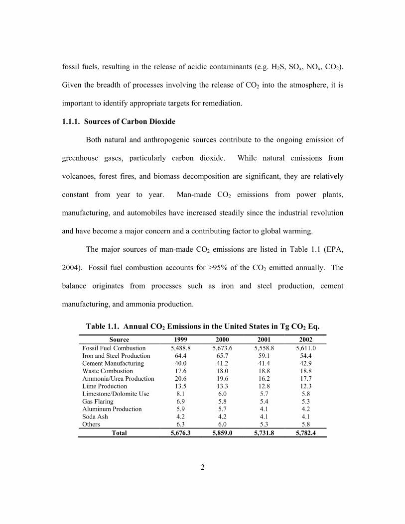
The major sources of man-made CO2 emissions are listed in Table 1.1 (EPA,
2004). Fossil fuel combustion accounts for >95% of the CO2 emitted annually. The
balance originates from processes such as iron and steel production, cement
manufacturing, and ammonia production.
Table 1.1. Annual CO2 Emissions in the United States in Tg CO2 Eq. Source 1999 2000 2001 2002
Fossil Fuel Combustion 5,488.8 5,673.6 5,558.8 5,611.0 Iron and Steel Production 64.4 65.7 59.1 54.4 Cement Manufacturing 40.0 41.2 41.4 42.9 Waste Combustion 17.6 18.0 18.8 18.8 Ammonia/Urea Production 20.6 19.6 16.2 17.7 Lime Production 13.5 13.3 12.8 12.3 Limestone/Dolomite Use 8.1 6.0 5.7 5.8 Gas Flaring 6.9 5.8 5.4 5.3 Aluminum Production 5.9 5.7 4.1 4.2 Soda Ash 4.2 4.2 4.1 4.1 Others 6.3 6.0 5.3 5.8
Total 5,676.3 5,859.0 5,731.8 5,782.4
3
Given the overwhelming percentage of emissions from fossil fuel combustion, it
becomes useful to analyze this source as individual sectors for simplified classification.
CO2 emissions are shown in Figure 1.1 for four point-source sectors, including
electricity generation and the residential, commercial, and industrial sectors (EPA,
2004). The transportation sector is also included.
Electricity generation accounts for 40.3% of the CO2 emissions from fossil fuel
combustion in the U.S. annually (EPA, 2004). Coal-fired power plants are the most
prominent point-source of CO2, constituting 83% of the power plant emissions, or one-
third of the total CO2 emitted annually from combustion sources. The industrial sector,
made up of ammonia production and other manufacturing processes, produces
approximately 17% of the total. Residential and commercial sectors, incorporating
mainly combustion for heating, combine to emit 11% of the total emissions.
Transportation makes up the remaining 32%.
Historically, coal has been the most significant source of electricity (EIA, 2002).
As shown in Figure 1.2, the use of coal as a power source has steadily risen since 1950.
Compared to other fossil fuels, the percentage of electricity produced from coal has also
steadily climbed from 66% in 1950 to 71% in 2002. Natural gas use has also risen and
petroleum combustion has remained fairly stable. Power from renewable sources and
nuclear power (not shown) have increased, but fossil fuel combustion still comprises
70% of the power production in the United States. It is apparent that coal has been and
continues to be the preferred fuel source.
4
Commercial4.2%
Residential6.7%
Power Plant - Petroleum1.3%
Industrial17.2%
Power Plant - Coal33.6%
Power Plant - Natural Gas5.4%
Transportation31.7%
Figure 1.1. CO2 Emissions from Fossil Fuel Combustion in the U.S. (2002), Total
Emissions: 5564.2 Tg CO2 Eq.
Year1950 1960 1970 1980 1990 2000
Elec
tric
ity G
ener
tatio
n(M
illio
n M
W-h
r)
0
500
1000
1500
2000
Coal
Natural Gas
Petroleum
Figure 1.2. History of Electricity Production from Fossil Fuels
5
Another important factor to consider is the efficiency of fuels for power
production. The efficiency is directly related to the amount of fuel, and thus the amount
of CO2 produced, necessary to produce given quantities of electricity. Of the three main
plant types, natural gas-fired plants are the most efficient (55 to 60%) and the cleanest
burning in terms of carbon, producing 0.45 kg CO2/kW-hr (IEA, 2001). Power
production from petroleum fuels gives 0.80 kg CO2/kW-hr. Coal-fired plants produce
the most carbon, approximately 0.96 kg CO2/kW-hr, and are only 40 to 50% efficient.
It is clear that the largest potential application for CO2 capture is coal-fired
power plants. Coal combustion is a well-established technology accounting for 50% of
the power in the U.S. The abundance of coal as a natural resource makes it a cheap,
readily available fuel. In short, it is the largest contributor to overall CO2 emissions and
trends suggest an expanding share of the power production market. Improvements in
capture technology for coal-fired power plants will be essential for making a significant
impact on U.S. CO2 emissions; therefore, most of the research presented in this work is
targeted to conditions of coal-fired power plants.
1.1.2. Carbon Dioxide Capture
A wide variety of processes have been developed for the removal of acidic
impurities from gas streams including membranes, cryogenics, adsorption, and, most
commonly, absorption into a chemical solvent (IEA, 2001). With membranes, high
purity streams are difficult to achieve, particularly on the scale of CO2 capture from
power plants. Cryogenic separation of CO2 would produce a high pressure, liquid CO2
stream, but the cost of refrigeration is often prohibitive and the removal of water would
6
be required, increasing the cost of the process. This technology is usually only
considered for highly concentrated CO2 streams. Adsorption has been tested, but a low
capacity and poor CO2 selectivity limit the potential for application to CO2 capture.
To date, capture by absorption methods provides the most economical response
to separating CO2 from bulk gas streams (IEA, 2001). Other methods may be applied in
niche applications and may be developed as long term solutions, but significant
advancements are required in these technologies before implementation in power plants
can be considered. For this reason, this work focuses on the development of a more
efficient absorption technology.
The absorption of CO2 into chemical or physical solvents is a well-developed
technology that has been applied to numerous commercial processes, including gas
treating and ammonia production (Kirk-Othmer, 2004). Much research has been
performed on this technology over the past 50 years, particularly on developing an
understanding of specific solvent characteristics. While a considerable body of work
has been published on specific amines, little work has been done on understanding or
representing complex mixtures which are often the most effective technologies.
1.1.3. Sinks and Sequestration of Carbon Dioxide
Following the successful capture of a concentrated carbon dioxide stream, the
gas must be stored or utilized with minimal loss to the atmosphere. The transportation
and storage of CO2 will be a significant cost associated with the remediation of
emissions; therefore, the development of efficient methods is critical to the application
of capture technology to industrial processes. The following discussion briefly
7
introduces a few of the currently recognized options for storage, though sequestration
technologies are outside the scope of this work.
Natural storage of CO2 is an ideal storage solution, but it will be difficult to
achieve efficiently. Naturally occurring sinks for CO2 include grasslands, forests, and
other biological processes. Natural sinks consume approximately 700 Tg CO2 Eq. per
year, far below that emitted into the atmosphere (EPA, 2004). Reforestation efforts are
being pursued to increase natural carbon sequestration; however, processes such as this
often require long time frames and large land areas to be effective.
Terrestrial locations are also a viable option for sequestering CO2. Various
geological formations have been proposed as suitable for storage, including depleted oil
reservoirs and saline reservoirs, each with various advantages (IEA, 2001). Depleted
oil reservoirs are well-defined storage options given the extensive exploration from oil
recovery. Saline reservoirs are naturally occurring aquifers containing salt water. The
CO2 would dissolve into the water and react with the salts to from other minerals.
Other sequestration technologies may serve as a useful process fluid as well as
viable storage options. Enhanced oil recovery (EOR) is one proven method of
sequestering CO2 while utilizing the gas to enhance the recovery of oil (IEA, 1995). In
this process, CO2 is injected into an oil reserve, improving the recovery of heavy oils
and geologically storing the CO2. In a similar process, CO2 may be injected into
unminable coal seams (IEA, 2001). The CO2 would adsorb onto the coal and displace
natural methane deposits, making the recovery of a fuel possible. The CO2 would
remain sequestered as long as the coal bed remained undisturbed. In both cases, the

8
requirements of a convenient source of high pressure CO2 and verification of long-term
CO2 fixation limit the potential of EOR as a wide-spread sequestration technology.
The ocean, the largest natural sink for CO2, has been proposed as a potential
storage location given its prominent place in the natural CO2 cycle (IEA, 2002). The
capacity for CO2 is large, but the physical rate of absorption limits the annual uptake of
CO2. In oceanic sequestration, the transport of CO2 is accelerated by direct dispersion
of the gas below the ocean surface, either by a fixed pipeline or ship. Concerns over the
use of this technology stem from the cost of transporting CO2 to the dispersion point
and the impact of pH changes on the biological life existing near the dispersion point.
1.2. Carbon Dioxide Capture by Absorption/Stripping
1.2.1. Technology Description
One of the most mature, and most researched, technologies for acid gas capture
from waste gas streams is an absorber/stripper process that uses a circulated chemical
solvent (Kohl and Reisenfeld, 1985). Processes such as this are currently used in
ammonia production and natural gas treating. There are several variations of this
flowsheet, including a temperature swing and an isothermal process.
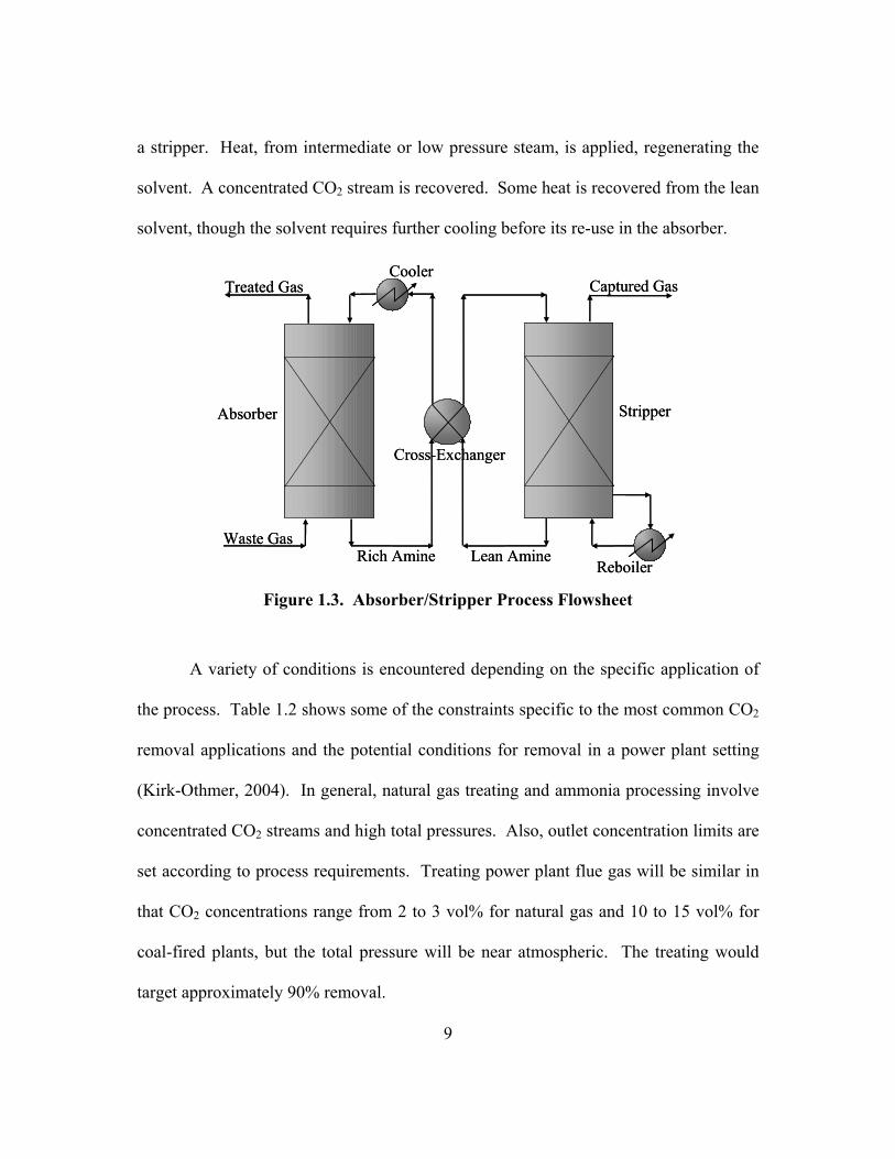
In the most common absorption process, the temperature swing variation (Figure
1.3), a waste gas stream containing CO2 enters the bottom of an absorber (Kohl and
Reisenfeld, 1985). The CO2 is removed and the treated gas exits the top of the column.
A CO2-lean solvent enters the top of the absorber and counter-currently contacts the gas
phase in packing or on trays. The CO2 is absorbed, and the rich solvent exits the
absorber. The rich solvent is pre-heated in a cross exchanger and pumped to the top of
9
a stripper. Heat, from intermediate or low pressure steam, is applied, regenerating the
solvent. A concentrated CO2 stream is recovered. Some heat is recovered from the lean
solvent, though the solvent requires further cooling before its re-use in the absorber.
Waste Gas
Captured GasTreated Gas
Rich Amine Lean AmineReboiler
Absorber Stripper
Cooler
Cross-Exchanger
Waste Gas
Captured GasTreated Gas
Rich Amine Lean AmineReboiler
Absorber Stripper
Cooler
Cross-Exchanger
Figure 1.3. Absorber/Stripper Process Flowsheet
A variety of conditions is encountered depending on the specific application of
the process. Table 1.2 shows some of the constraints specific to the most common CO2
removal applications and the potential conditions for removal in a power plant setting
(Kirk-Othmer, 2004). In general, natural gas treating and ammonia processing involve
concentrated CO2 streams and high total pressures. Also, outlet concentration limits are
set according to process requirements. Treating power plant flue gas will be similar in
that CO2 concentrations range from 2 to 3 vol% for natural gas and 10 to 15 vol% for
coal-fired plants, but the total pressure will be near atmospheric. The treating would
target approximately 90% removal.

10
Table 1.2. Process Conditions in Absorber/Stripper Applications to CO2 Capture
Process Inlet CO2 (vol %)
Outlet CO2 (vol %)
PTOT (atm)
Natural Gas 0 � 50 1 � 2 10 � 70 Ammonia 17 � 19 0.01 � 0.2 30 Coal Power Plant 10 � 15 1 � 1.5 1 � 1.3 Natural Gas Power Plant 2 � 3 0.2 � 0.3 1 � 1.3
1.2.2. Factors in Cost
While CO2 capture has been proposed for power plant applications, the cost of
implementing this technology is currently prohibitive. Estimates suggest an 80%
increase in the cost of electricity from coal fired power plants with CO2 capture (Rubin
et al., 2004). The components of this cost must be understood to effectively improve
upon the process and move towards commercialization.
In a study of a standardized, coal-fired power plant (including flue gas
desulfurization), Rao and Rubin (2002) categorize and quantify contributions to the
overall cost of CO2 capture by 30 wt% monoethanolamine (MEA), considered state-of-
the-art technology, and subsequent sequestration. The capture and compression of CO2
accounts for 80% of the total cost. The balance of the cost (20%) is due to
transportation and sequestration. The obvious obstacle for implementation is the
capture of CO2; therefore, a significant opportunity for reducing costs lies with
improving the capture process.
Within the capture process, compression accounts for 34% of the cost (Rao and
Rubin, 2002). The efficiency of this component will be dictated by pressure and
temperature of the concentrated gas stream. Approximately 17% of the total operating
11
cost is from the circulation of the solvent and gas through the columns by pumps and
blowers. Minimizing pressure drop, and consequently packing height, may be an
important consideration in reducing cost.
The most significant cost of CO2 capture is the energy requirement for solvent
regeneration, making up 49% of the total capture cost. The regeneration energy
required can be estimated from three solvent properties, as discussed below. Though
others may be important, the following are the most significant factors in determining
the cost regeneration (Rochelle et al., 2001).
The capacity of a solvent is a measure of the amount of CO2 absorbed per unit of
solvent. The capacity defines the total CO2 concentration change over a set range of
equilibrium partial pressures, reflecting the vapor-liquid equilibrium characteristics of
the solvent. A high solvent capacity indicates that more CO2 can be absorbed/stripped
with a set amount of energy. Thus, given a constant circulation rate, the process
becomes more efficient.
The heat of CO2 absorption is another important solvent property. As CO2
reacts with the solvent in the absorber, heat is liberated. Excluding latent and sensible
heat, an amount of heat equivalent to this must be applied to reverse the reaction and
remove CO2 from the solution in the stripper. The application of this property to energy
assessments is straightforward in that a reduction ordinarily lowers the required energy
per mol of CO2.
Improving the rate of CO2 absorption into a solvent impacts several facets of the
process and provides additional process flexibility. A faster rate of absorption, for a
12
given separation, allows the reduction of the liquid flowrate or a reduction in packing
height, saving costs associated with liquid holdup, pressure drop, and latent heat.
Alternatively, the absorber can be run closer to equilibrium, which may be the more
favorable option depending on the solvent capacity.
An improved solvent for CO2 capture can result in significant energy savings.
The performance of potential solvents should be screened and compared according to
improvements made in the aforementioned properties.
1.2.3. Solvents
Many solvents have been applied to gas treating, but the most effective are
generally considered to be aqueous amines or hot potassium carbonate (hotpot)
solvents. The variety of amines is endless, but some of the more common are shown in
Table 1.3. Amines have an advantage over the hotpot process in that the absorption rate
of CO2 by amines is fast; however, the heat of absorption is also high. In contrast,
absorption into potassium carbonate has a heat of absorption similar to physical
solvents, but is limited by slow absorption rates.
In high pressure applications, physical solvents are utilized. Some of the more
common solvents are Selexol, Rectisol, and Purisol (Kirk-Othmer, 2004). Because
physical solvents do not react with CO2, the solvent is not consumed at high partial
pressures. Additionally, the heat of absorption is limited to the enthalpy of physical
absorption, much less than the reactive solvents. The processes are limited by
selectivity and slow rates of absorption.
13
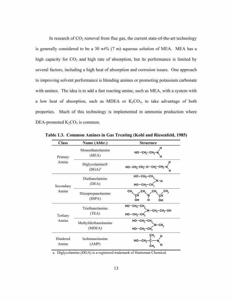
In research of CO2 removal from flue gas, the current state-of-the-art technology
is generally considered to be a 30 wt% (7 m) aqueous solution of MEA. MEA has a
high capacity for CO2 and high rate of absorption, but its performance is limited by
several factors, including a high heat of absorption and corrosion issues. One approach
to improving solvent performance is blending amines or promoting potassium carbonate
with amines. The idea is to add a fast reacting amine, such as MEA, with a system with
a low heat of absorption, such as MDEA or K2CO3, to take advantage of both
properties. Much of this technology is implemented in ammonia production where
DEA-promoted K2CO3 is common.
Table 1.3. Common Amines in Gas Treating (Kohl and Riesenfeld, 1985)
Class Name (Abbr.) Structure
Monoethanolamine (MEA)
OH CH2 CH2 NH
H
Primary Amine Diglycolamine®
(DGA)a O CH2 CH2 N
H
HCH2CH2OH
Diethanolamine (DEA) OH CH2 CH2
OH CH2 CH2
N H
Secondary Amine Diisopropanolamine
(DIPA) OHCH
CH2N
CH2
HCH
CH3
OH
CH3
Triethanolamine (TEA) OH CH2 CH2
OH CH2 CH2
N OHCH2CH2
Tertiary Amine Methyldiethanolamine
(MDEA) OH CH2 CH2
OH CH2 CH2N CH3
Hindered Amine
Isobutanolamine (AMP)
OH CH2 C NH
H
CH3
CH3
a. Diglycolamine (DGA) is a registered trademark of Huntsman Chemical.
14
1.3. Potassium Carbonate/Piperazine for Carbon Dioxide Capture
1.3.1. Solvent Description
This work proposes a new solvent, containing concentrated aqueous potassium
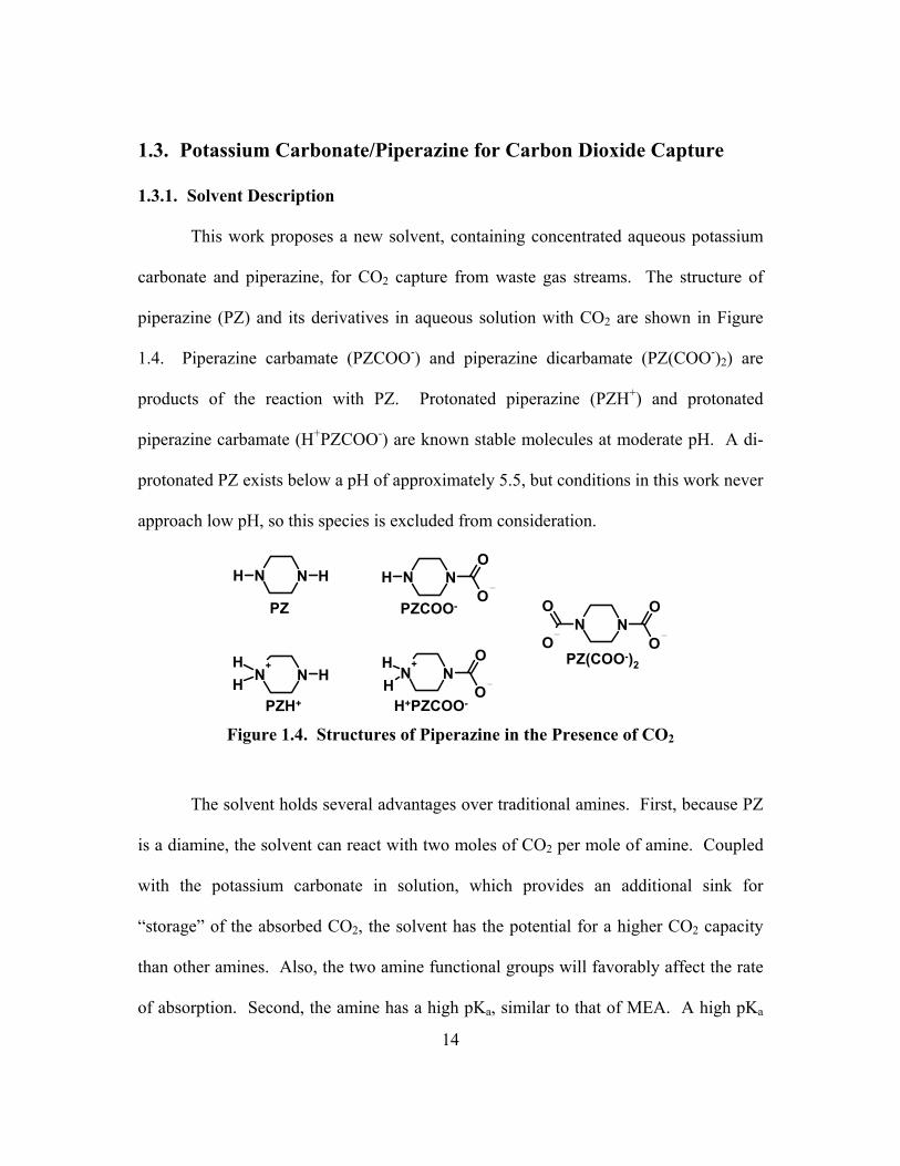
carbonate and piperazine, for CO2 capture from waste gas streams. The structure of
piperazine (PZ) and its derivatives in aqueous solution with CO2 are shown in Figure
1.4. Piperazine carbamate (PZCOO-) and piperazine dicarbamate (PZ(COO-)2) are
products of the reaction with PZ. Protonated piperazine (PZH+) and protonated
piperazine carbamate (H+PZCOO-) are known stable molecules at moderate pH. A di-
protonated PZ exists below a pH of approximately 5.5, but conditions in this work never
approach low pH, so this species is excluded from consideration.
N NH H N NO
OH
N+
NO
OHH
N NO
O O
O
N+
NH
HH
PZ PZCOO-
PZ(COO-)2
PZH+ H+PZCOO- Figure 1.4. Structures of Piperazine in the Presence of CO2
The solvent holds several advantages over traditional amines. First, because PZ
is a diamine, the solvent can react with two moles of CO2 per mole of amine. Coupled
with the potassium carbonate in solution, which provides an additional sink for
�storage� of the absorbed CO2, the solvent has the potential for a higher CO2 capacity
than other amines. Also, the two amine functional groups will favorably affect the rate
of absorption. Second, the amine has a high pKa, similar to that of MEA. A high pKa
15
generally translates into a fast rate of absorption. Third, the large quantity of
carbonate/bicarbonate in solution serves as a buffer, reducing the protonation of the
amine and leaving more amine available for reaction with CO2.
1.3.2. Research Needs
Several critical questions should be addressed to develop a better understanding
of K+/PZ mixtures and amines as applied to CO2 capture. As discussed in Section
1.2.2., there is a need to quantify several critical performance characteristics. While
quantifying specific performance characteristics, it becomes beneficial to further
develop the underlying fundamental science.
Thus far, little research has been published on the thermodynamics or kinetics of
polyamines or salt-amine mixtures. Research on vapor-liquid equilibrium (VLE) of
CO2 in the solvent will define capacity and heats of absorption. Of fundamental interest
in the understanding of the thermodynamics is a description of amine speciation with
CO2 and, for PZ, an identification of differences resulting from the unique, heterocyclic
ring structure. It is also important to identify VLE benefits by using similar molecules.
In promoted K2CO3 systems, the impact of high ionic strength on equilibria is largely
unknown. An effective thermodynamic representation of K+/PZ will improve the
fundamental understanding of other amine solutions and mixtures.
Addressing the rate of absorption will complete the understanding of overall
solvent performance. Investigations of the rate behavior will also support previous
theories of amine reactions with CO2. Verifying a reaction mechanism and supporting
the Brønsted theory of base catalysis will improve the kinetic representation of amine

16
systems. Also, research on kinetics in K+/PZ will improve the modeling of neutral salt
effects important in high ionic strength environments. Additionally, validating an
effective absorption rate model will aid the general understanding and methods for
describing reactive transport in a complex system.
1.3.3. Previous Work
Some prior work on PZ as a CO2 absorbent has been published and is
summarized in Table 1.4, but most of the data are at conditions outside the range of
interest for this work. Most of the VLE data are at CO2 loadings above 0.75 mol
CO2/mol amine, compared to the 0.1 to 0.5 range encountered in flue gas treating.
Bishnoi (2000) presents some data on PZ, but the majority of his work focuses on
PZ/MDEA blends. The most comprehensive study of aqueous PZ is given by
Ermatchkov et al. (2003) who reports speciation data for a wide range of conditions.
Table 1.4. Summary of Previous Work on Piperazine
Solvent [PZ] (M) T (oC) CO2 Loading Source Data Type
0.2 � 0.6 25 - 70 0.0 � 1.0 Bishnoi (2000) NMR, VLE, Rate 0.1 � 1.45 10 � 60 0.0 � 1.0 Ermatchkov et al. (2003) NMR
2 � 4 40 � 120 > 0.75 Kamps et al. (2003) VLE Aq. PZ
0.1 � 1.0 20 � 50 > 0.8 Aroua and Salleh (2004) VLE 0.6 25 � 70 0.0 � 0.7 Bishnoi (2002,2002) NMR, VLE, Rate PZ +
Amine 0.0 � 1.2 40 - 60 0.0 � 0.5 Dang (2001) VLE, Rate Amine + K2CO3
N/A Various Various Various, See Section 2.2.6. VLE, Rate
Though general studies of the solvent performance of amine/K2CO3 solvents are
common, detailed data on thermodynamics and kinetics are not available in the open
literature. Properties of PZ/K2CO3 have not been previously explored. This work
17
builds on the data set for aqueous PZ and expands the solvent to include concentrated
K2CO3.
Other work, though not addressing PZ specifically, is closely related to this
investigation through methods and modeling techniques and should be mentioned.
Austgen (1989) developed the rigorous thermodynamic model used in this work and
applied it to modeling MEA- and DEA-promoted MDEA. Glasscock (1990) initiated a
study on the modeling of CO2 absorption into DEA and DEA/MDEA. These works
demonstrate the ability of various modeling techniques to effectively represent amine
mixtures over a broad range of conditions, though none specifically address high ionic
strength solvents. Also, the prior work in this area focuses on simpler solvent systems;
this work will attempt to extend these methods to a more complex application.
1.3.4. Objectives and Scope
Following the above rational for needed research on this solvent and in the
general field of gas treating with amines, this work strives to satisfy several critical
objectives, encompassing both scientific explorations and practical considerations:
1. Quantify and model fundamental thermodynamic properties that
determine solvent behavior over conditions relevant to gas treating.
2. Determine the rate of CO2 absorption into K+/PZ mixtures and relate
the performance to kinetic theory in other amine solvents.
3. Investigate the feasibility of applying the K+/PZ mixture in an
industrial gas treating process and identify controlling variables.
18
4. Anticipate practical limitations of applying the solvent to CO2 capture
in the proposed process.
The scope of the proposed work encompasses, to a large extent, conditions that would
be encountered by applying the solvent to large-scale CO2 removal from flue gas. That
is, the temperature range of interest is from 40 to 120oC and the gas phase CO2
concentration is 0.1 to 10%.
Objective 1 is satisfied by experimental and modeling investigations of
important thermodynamic properties. Data on the vapor-liquid equilibrium of CO2 over
0.0 to 6.2 m K+ and 0.0 to 3.6 m PZ have been measured in a wetted-wall column at 40
to 110oC. The equilibrium speciation of PZ in 2.5 to 6.2 m K+ and 0.6 to 3.6 m PZ was
measured using proton nuclear magnetic resonance spectroscopy. The physical
solubility of CO2 in K+/PZ mixtures (up to 5.0 m K+ and 2.5 m PZ) was determined by
the N2O analogy.
A rigorous thermodynamic model, based on the electrolyte non-random two-
liquid (ENRTL) theory, was developed using the model originally coded by Austgen
(1989). The model was extended to include K+ and PZ and used, in conjunction with
the experimental measurements, to develop a broad picture of thermodynamic behavior
and to infer practical consequences of that behavior. Scientific conclusions concerning
the stability of PZ carbamates and the pKa of species were formed. Enthalpies predicted
by the model are comparable to literature values and used to generalize the behavior of
aqueous PZ and K+/PZ. The influence of ionic strength on thermodynamic behavior
was successfully correlated and interpreted with the activity coefficient model.
19
The second objective was met with measurements of the rate of CO2 absorption
in the wetted-wall column in a variety of solvents (0.0 to 6.2 m K+ and 0.6 to 3.6 m PZ)
between 25 and 110oC. A kinetic model, based on the model of Bishnoi (2000), was
developed from the observed behavior to model the boundary layer for the absorption of
CO2 into K+/PZ.
Using the data and the model, rate constants describing the reaction of PZ with
CO2 were regressed as part of a termolecular reaction mechanism. Furthermore, the
rate constants were structured to satisfy the Brønsted theory of acid-base catalysis.
Given the high ionic strength of the solvent, studies into neutral salt effects were
deemed appropriate. The influence of salt on the reaction rate was interpreted and
generalized. The model was used to correlate the flux of CO2 into the solvent under
various conditions and to arrive at conclusions concerning generalized rate behavior and
important parameters for mass transfer.
Objective 3 is satisfied from interpretations of the thermodynamic and kinetic
behavior as understood from experimental investigations. From the electrolyte NRTL
model, correlations of VLE behavior were used to estimate the CO2 capacity of the
solvent and the heat of absorption. The rigorous rate model was applied to
understanding the importance of kinetics and diffusion parameters. In comparing the
rate of absorption to the instantaneous rate and gas film resistance contributions,
conclusions about the performance of the solvent in an industrial process are achieved.
The fourth objective of this work includes practical considerations of solvent
development. A basic study of the solid solubility of K+/PZ mixtures was initiated to

20
determine viable solvent compositions. Solubility limits were quantified in
concentrated mixtures of K2CO3/PZ and KHCO3/PZ at 25 and 40oC. The solubility
limits also serve as an important addition to the thermodynamic investigations.
Physical properties, such as density and viscosity, have been measured and reported to
improve modeling and interpretation of fluid dependent parameters.
21
Equation Chapter 2 Section 1
Chapter 2: Literature Review
This chapter introduces basic theory and literature pertaining to a study of CO2
absorption by aqueous amines. A brief discussion on mass transfer with chemical
reactions is presented, highlighting basic terminology. Approximations and limiting
conditions are also discussed. Generalized equilibrium and rate behavior of amine
solvents is presented with a particular emphasis on promoted-K2CO3 and prior work in
the area. Research on acid-base catalysis theory and the effect of neutral salts are
reviewed in the context of application to CO2 reactions with amines.
2.1. Mass Transfer with Fast Chemical Reaction
2.1.1. Mass Transfer Theory
Detailed information on the transport of molecular species is commonly
modeled with a microscopic material balance. In the simplest form, one species
22
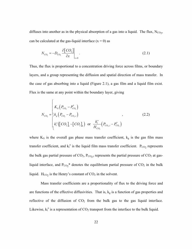
diffuses into another as in the physical absorption of a gas into a liquid. The flux, NCO2,
can be calculated at the gas-liquid interface (x = 0) as
[ ]2 2
2
0CO CO
x
CON D
x=
∂= −
∂. (2.1)
Thus, the flux is proportional to a concentration driving force across films, or boundary
layers, and a group representing the diffusion and spatial direction of mass transfer. In
the case of gas absorbing into a liquid (Figure 2.1), a gas film and a liquid film exist.
Flux is the same at any point within the boundary layer, giving
( )( )[ ] [ ]( ) ( )
2 2
2 2 2
2 2
2
*
,
*2 2 , or
G CO CO
CO g CO CO i
oo ll CO i COi b
CO
K P P
N k P P
kk CO CO P PH
−= − − −
, (2.2)
where KG is the overall gas phase mass transfer coefficient, kg is the gas film mass
transfer coefficient, and klo is the liquid film mass transfer coefficient. PCO2 represents
the bulk gas partial pressure of CO2, PCO2,i represents the partial pressure of CO2 at gas-
liquid interface, and PCO2* denotes the equilibrium partial pressure of CO2 in the bulk
liquid. HCO2 is the Henry�s constant of CO2 in the solvent.
Mass transfer coefficients are a proportionality of flux to the driving force and
are functions of the effective diffusivities. That is, kg is a function of gas properties and
reflective of the diffusion of CO2 from the bulk gas to the gas liquid interface.
Likewise, klo is a representation of CO2 transport from the interface to the bulk liquid.
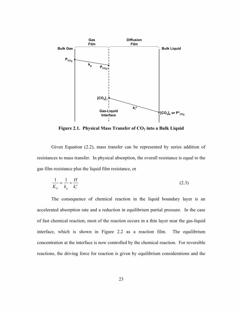
23
PCO2
PCO2,i
[CO2]b or P*CO2
[CO2],i
Gas-LiquidInterface
Bulk Gas Bulk Liquid
GasFilm
klo
kg
DiffusionFilm
Figure 2.1. Physical Mass Transfer of CO2 into a Bulk Liquid
Given Equation (2.2), mass transfer can be represented by series addition of
resistances to mass transfer. In physical absorption, the overall resistance is equal to the
gas film resistance plus the liquid film resistance, or
1 1o
G g l
HK k k
= + (2.3)
The consequence of chemical reaction in the liquid boundary layer is an
accelerated absorption rate and a reduction in equilibrium partial pressure. In the case
of fast chemical reaction, most of the reaction occurs in a thin layer near the gas-liquid
interface, which is shown in Figure 2.2 as a reaction film. The equilibrium
concentration at the interface is now controlled by the chemical reaction. For reversible
reactions, the driving force for reaction is given by equilibrium considerations and the

24
diffusion of CO2 to the reaction film. See Section 2.1.3. A representation can again be
written as a series resistance
[ ]2 2
*
, 2
1 1 1CO COo o
G g l l PROD T
H PK k Ek k CO
∂= + +
∂ (2.4)
where [ ]2
*2CO T
P CO∂ ∂ gives the slope of the equilibrium curve. This term is essentially
the instantaneous, or diffusion controlled, transport of CO2. E is an enhancement factor
accounting for the reaction of CO2 and is defined as the flux of CO2 with reaction
normalized by the flux of CO2 by physical absorption. In this work, the enhancement
factor is referred to as a gas phase mass transfer coefficient across the liquid film, called
a normalized flux or kg�.
2
'ol
gCO
EkkH
= (2.5)
PCO2
PCO2,i
[CO2]b or P*CO2
[CO2]*
[CO2],i
Gas-LiquidInterface
Bulk Gas Bulk Liquid
GasFilm
klo
RxnFilm
kg
DiffusionFilm
Figure 2.2. Mass Transfer of CO2 into a Bulk Liquid with Fast Chemical Reaction
25
2.1.2. Mass Transfer Models
One of the earliest, and simplest, mass transfer models is called film theory and
was first proposed by Lewis and Whitman (1924). Film theory is a steady-state model,
resulting in a simple representation of mass transfer in the boundary layer. The
assumption is mass transfer occurs across a stagnant film of given thickness δ.
A physical mass transfer coefficient, klo, gives a proportional dependence of flux
on the diffusion coefficient, which disagrees with most experimental data.
Additionally, the film model predicts discontinuities at the gas-liquid interface and at δ,
implying a more complicated model of mass transfer is required to accurately describe
diffusion of species in a boundary layer.
Two other theories have garnered widespread use due their applicability to a
range of problems. The Higbie penetration theory (Higbie, 1935) and the surface
renewal theory (Danckwerts, 1951) are unsteady-state theories that assume molecules
contact the gas-liquid interface for various amounts of time, yielding a contact time
distribution. Both theories produce a flux that is dependent on the square root of the
diffusivities, giving a better representation of observed behavior, but they are more
complicated to solve.
The eddy diffusivity theory (Equation (2.6)), proposed by King (1966), is a
steady-state theory that assumes a significant convective contribution to the diffusion of
species in the boundary layer. Near the interface, diffusion processes are dominant.
Approaching the bulk solution results in greater contributions from convective fluid
movement, or eddies.
26
( ) [ ]2
22 0CO
COD x
x xε
∂∂+ = ∂ ∂
(2.6)
Glasscock (1990) showed that the eddy diffusivity theory gives a solution within
5% of the surface renewal or penetration theory without the complications of time
dependence. For this reason, Bishnoi (2000) chose this theory as the basis for his mass
transfer model, which is incorporated into this work.
2.1.3. Reversible Reactions
The reactions considered in this work are reversible, and require special
consideration of the appropriate driving force. Given a simple, reversible reaction of a
reactant, R, with the dissolved gas, CO2,
2f
r
k
kR CO P→+ ← , (2.7)
the overall expression for rate is
[ ][ ] [ ]2f rr k R CO k P= − . (2.8)
An equilibrium constant, assuming [R] >> [CO2], can also be defined as
[ ][ ][ ]*
2
f
r
k PK
k R CO= = , (2.9)
where * indicates the concentration in equilibrium as defined by the above expression.
The rate is now given in terms of the driving force imposed by the actual concentration
and the equilibrium concentration of the dissolved gas.
[ ] [ ] [ ]( )*2 2 2r k R CO CO= − (2.10)
27
The reversible rate expression can, therefore, be calculated using the equilibrium
constant.
[ ] [ ] [ ][ ]2 2
Pr k R CO
K R
= −
(2.11)
2.1.4. Pseudo-First Order Reaction
The complexity of representing mass transfer with fast chemical reactions as an
analytical expression has led to the development of useful simplifications. One such
simplification is the pseudo-first order approximation. This approximation assumes that
the liquid reactant concentration is constant throughout the boundary layer, eliminating
the need for rigorous accounting of speciation in the reactive boundary layer. In other
words, the reaction rate can be represented by the bulk solution composition.
The pseudo-first order assumption is applied as follows. The concentration
profile of CO2 reacting with an amine in a second order reaction is given by
[ ] [ ][ ]2
22
2 22 0CO
COD k Am CO
x∂
− =∂
. (2.12)
Assuming the amine concentration across the reactive boundary layer is constant and
equal to the bulk liquid concentration,
[ ] [ ]2
22
1 22 0CO
COD k CO
x∂
− =∂
, (2.13)
where k1 is a pseudo-first order rate constant representing k2[Am]b.
The solution to this equation, for reversible reactions, is
[ ] ( )2
2 2 2
2
2 *,
CO bCO CO i CO
CO
D k AmN P P
H= − . (2.14)

28
The subscript b indicates bulk solution composition. The resulting expression for the
normalized flux is
[ ]2
2
2',
CO bg PFO
CO
D k Amk
H= . (2.15)
This approximation requires that the concentration of the amine and PCO2* at the
gas-liquid interface be approximately equal to those in the bulk solution. Thus, the flux
must be low relative to the reactant and product concentrations. An increase in reaction
kinetics relative to diffusion processes may result in the depletion of the reactant, or an
accumulation of the products, at the gas-liquid interface. Likewise, a high driving force
may deplete the reactant and introduce large errors into this approximation.
2.1.5. Instantaneous Reactions
A special case of mass transfer with chemical reaction is one where the reaction
occurs fast enough to be considered instantaneous with respect to the diffusion process.
Some reactions between gases and liquids are commonly represented as instantaneous,
such as the absorption of NH3 by aqueous HCl and H2S by an alkaline solution. Under
some circumstances, describing the absorption process of CO2 by an amine as
instantaneous may be appropriate. Generally, this occurs at high temperatures where
kinetics have increased or at high loadings where the accumulation of CO2 products
places diffusion limitations on the reaction.
Consider a simplified situation in which
12
kCO R P+ → (2.16)
29
and k1 → ∞ (the reaction is instantaneous). The reaction of CO2 with R occurs at some
distance, δ, from the gas-liquid interface. Conditions require that R diffuse to and P
diffuse away from the reaction plane at least as fast as CO2 reaches it, resulting in
[ ] [ ][ ]
2
2
2
*2
*2
1CO R bCO
CO
D CO D RN
D COδ
= +
. (2.17)
Or, if film theory applies,
[ ] [ ][ ]2
2
*2 *
2
1 Ro bCO l
CO
D RN k CO
D CO
= +
. (2.18)
For the circumstance of sparingly soluble gas in a liquid, the expression is simplified to
[ ]2
2
Ro bCO l
CO
D RN k
D= . (2.19)
This approximation is of practical importance for several reasons. First, if the
reaction is instantaneous, the rate can be modeled with a simple model with no
consideration of kinetics. Second, the influence of the gas film resistance can be
quantified relative to the reaction rate for modeling absorber/stripper processes. Third,
the prediction of instantaneous behavior relative to various reactions allows the
determination of rate limiting behavior.
Similar solutions can be found for more complex reactions. For amines reacting
with CO2, several representations for instantaneous reaction can be derived. The
condition where all reactions are considered instantaneous will be referred to as the
global instantaneous case, designated by GBL,INST. With a small driving force, an
approximate solution to this condition can be calculated from equilibrium behavior as

30
[ ] ( )2 2 2
2 2
2 *, , ,*
o P TCO GBL INST l CO i CO
CO CO
CODN k P PD P
∂= −
∂, (2.20)
where DP represents the diffusion coefficients of the reaction products and [CO2]Τ is the
molar liquid CO2 concentration.
Other instantaneous reactions can be considered to determine the contribution of
a particular class of reactions to the overall reaction rate. An instantaneous flux for the
formation of amine carbamates can be defined as
( )2 2, , limAm b
Am b
CO PZ INST COkN N
− →∞=
∑∑. (2.21)
A comparison to the global instantaneous case reveals the potential limiting reactions
under given conditions.
2.2. Solvents for CO2 Absorption
The following discussion covers the major thermodynamic and kinetic
conclusions for various types of amines and presents key findings that are applied in
interpreting results of this work. The review is not intended to be a comprehensive
listing of all work done in the area. Several authors have compiled detailed literature
reviews on amines. See Mahajani and Joshi (1988), Versteeg et al. (1996), and
Rochelle et al. (2001) for more detail.
2.2.1. Potassium Carbonate
The value of potassium carbonate as a CO2 absorbent has been recognized since
the early 1900�s. The process evolved over the years into a viable commercial process,
often used in treating synthesis gas (Benson and Field, 1959). The preferred
31
embodiment is a 40 wt% K2CO3 solution in an isothermal absorber/stripper at 100oC
and 15 to 20 atm.
Much of the commercial validation was done by Benson et al. (1954) and
Benson et al. (1956). These two studies show important pilot plant characterization of
hot potassium carbonate (hotpot) versus aqueous MEA and conclude that, under
specific configurations, hotpot is an efficient CO2 absorbent.
The absorption of CO2 into aqueous K2CO3 is commonly represented by the
overall reaction
( )23 2 2 32CO H O CO aq HCO− −→+ + ← , (2.22)
though the reaction is usually described in terms of two parallel, reversible reactions.
( )2 3CO aq OH HCO− −→+ ← (2.23)
23 3 2HCO OH CO H O− − −→+ +← (2.24)
Since the reaction with hydroxide is the rate-limiting step, the reaction rate is
represented as a second order rate expression.
[ ]2 2CO OH
r k OH CO−− = (2.25)
This reaction, though important to the solution equilibrium, is generally much slower
than aqueous amines, limiting its application in processes requiring a high percentage of
removal. It is often advantageous to add a promoter to increase the absorption rate. The
energy required to reverse the reaction is typically less than that required for amine
solvents.
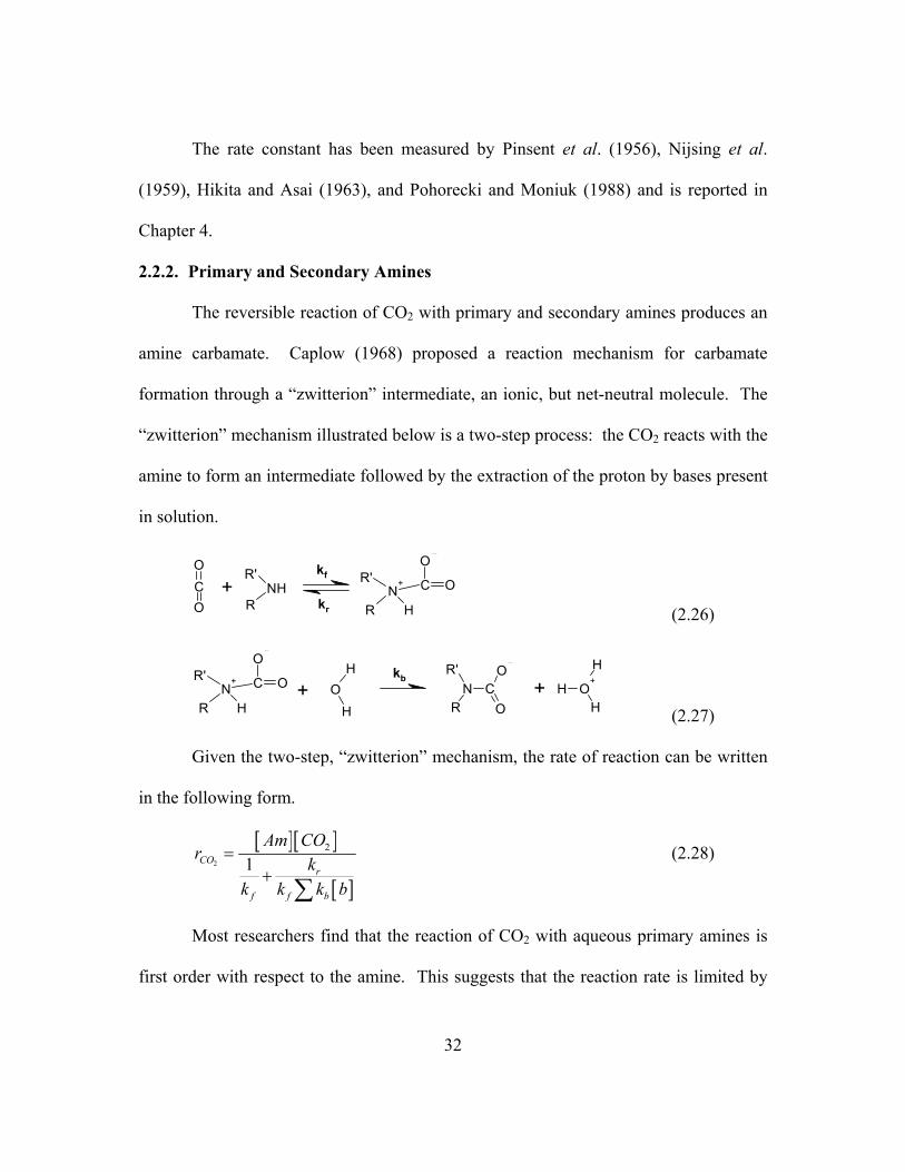
32
The rate constant has been measured by Pinsent et al. (1956), Nijsing et al.
(1959), Hikita and Asai (1963), and Pohorecki and Moniuk (1988) and is reported in
Chapter 4.
2.2.2. Primary and Secondary Amines
The reversible reaction of CO2 with primary and secondary amines produces an
amine carbamate. Caplow (1968) proposed a reaction mechanism for carbamate
formation through a �zwitterion� intermediate, an ionic, but net-neutral molecule. The
�zwitterion� mechanism illustrated below is a two-step process: the CO2 reacts with the
amine to form an intermediate followed by the extraction of the proton by bases present
in solution.
CO
ONH
R'
RN
+R'
R
C O
O
H+
kf
kr (2.26)
N+R'
R
C O
O
HN
R'
RC
O
OO
H
HO
+
H
H
H+ +kb
(2.27)
Given the two-step, �zwitterion� mechanism, the rate of reaction can be written
in the following form.
[ ][ ]
[ ]2
2
1COr
f f b
Am COr k
k k k b
=+
∑ (2.28)
Most researchers find that the reaction of CO2 with aqueous primary amines is
first order with respect to the amine. This suggests that the reaction rate is limited by
33
the formation of the zwitterion, kb→∞. In this case, the rate expression can be
simplified to
[ ][ ]2 2CO fr k Am CO= . (2.29)
Researchers also find that the CO2 reaction with secondary amines frequently
approaches a second-order reaction with respect to the amine. Assuming the extraction
of the proton by a base is rate-limiting, or Σkb[b] << kr, Equation (2.28) can be
simplified to
[ ][ ][ ]2Am bb
r k Am b CO−= ∑ , (2.30)
where kAm-b represents the combination of kf, kr, and kb. For example, if PZ is the
reacting amine and water is the base, the nomenclature is
2
2
f H OPZ H O
r
k kk
k− = . (2.31)
Recent work by Crooks and Donnellan (1989) suggests the use of a single-step,
termolecular mechanism to describe the reaction. The rate expression resulting from
the termolecular mechanism is identical to Equation (2.30). The authors argue that
while the �zwitterion� mechanism explains observed reaction rates, the mechanism is
not thermodynamically consistent and the physical significance of the �zwitterion� is
questionable. This view is supported by the recent ab initio study of carbamate
formation by da Silva and Svendsen (2004). Because there is no direct evidence that an
intermediate exists, the reaction can be represented as termolecular with no adverse
effects (Benson, 1960).
34
Several investigations of amine systems utilize the �zwitterion� mechanism in
its entirety to describe amine kinetics, but the values of kf often have questionable
significance or little impact on the reaction rate (Blauwhoff et al., 1984; Bosch et al.,
1990; Littel et al., 1992a; Kumar et al., 2003). With a termolecular interpretation,
varying orders of reaction can be obtained if the amine is also considered an acting
base; therefore, regardless of the chosen mechanism, an equally effective representation
of the reaction rate can be obtained. While it is difficult to make conclusions
concerning the actual mechanism, the termolecular mechanism is comparably attractive
in its simplicity and has been chosen to represent the data in this work.
Equilibrium representations of primary and secondary amines in water can be
relatively complex. In addition to the equilibria of components in water, the carbamate
and protonation of the amine must be considered.
2 2 3Am CO H O AmCOO H O− +→+ + +← (2.32)
2 3AmH H O Am H O+ +→+ +← (2.33)
From carbamate formation and subsequent protonation, primary and secondary amines
can theoretically absorb 0.5 mol CO2/mol amine and are somewhat limited in their
capacity to absorb CO2. The carbamate reaction also has a high heat of absorption,
making the solution difficult to regenerate.
There is an extensive collection of literature available on the kinetics of CO2
with primary amines, particularly MEA. Jensen et al. (1954), Clarke (1964),
Danckwerts and Sharma (1966), Sada et al. (1976b), Hikita et al. (1977), and Penny and

35
Ritter (1983) report second-order rate constants for MEA of approximately 7000
m3/kmol-s. DGA is reported to have a rate constant of 5000 m3/kmol-s (Alper, 1990a;
Littel et al., 1992b).
Secondary amines give similar rates as primary amines, but rates are usually
reported in terms of the �zwitterion� mechanism. Kinetics of DEA and DIPA are
reported by Sada et al. (1976a), Hikita et al. (1977), Laddha and Danckwerts (1981),
Versteeg and van Swaaij (1988a), and Littel et al. (1992a).
2.2.3. Tertiary Amines
The reaction of tertiary amines with CO2 differs significantly from primary or
secondary amines in that an amine carbamate is not formed. Instead, the reaction
produces a protonated amine and bicarbonate ion, resulting in a high capacity and a low
heat of absorption. The reaction is consistent with a single-step mechanism, as with
primary or secondary amines, but the products resemble a homogeneous catalysis of
CO2 hydrolysis. The absorption rate for tertiary amines is considerably slower and
water must be present for this reaction to proceed.
NR"
RR' O
H
HCO
ON
+R"
RR' H OH C
O
O+ + +
(2.34)
The rate of this reaction is typically represented with a second-order reaction.
[ ][ ]2 2 2COr k Am CO= (2.35)
Several tertiary amines have been investigated for CO2 absorption and selective
removal of H2S, including TEA and DMMEA (dimethylmonoethanolamine), though
36
MDEA is the most common used in gas treating. Investigations of MDEA kinetics
include work by Blauwhoff et al. (1984), Versteeg and van Swaaij (1988a), Toman and
Rochelle (1989), and Rinker et al. (1995). An average second-order rate constant is 4
m3/kmol-s. Results for TEA are similar, giving a rate constant of approximately 2
m3/kmol-s (Sada et al., 1976a; Donaldson and Nguyen, 1980; Crooks and Donnellan,
1990; Littel et al., 1990b).
2.2.4. Hindered Amines
Hindered amines have been developed for use in a number of processes
including CO2 removal. Hindered amines are primary or secondary amines whose
structure inhibits the formation of carbamate species. A formal definition has been
adopted as �a primary amine in which the amino group is attached to a tertiary carbon,
or a secondary amine in which the amino group is attached to a secondary or a tertiary
carbon atom� (Sartori and Savage, 1983). Some solvents contain severely hindered
amines for the selective removal of H2S.
In representing the interaction of CO2 with hindered amines, several reactions
must be considered. The reaction of CO2 with moderately hindered amines includes the
formation of a carbamate species as in the case of non-hindered amines.
2 2 3Am H O CO AmCOO H O− +→+ + +← (2.36)
This reaction is often significantly slower and contributes less to the overall reaction
rate than for primary or secondary amines due to the low carbamate stability. It is
theorized that the subsequent decomposition of the carbamate to bicarbonate may
contribute to the reaction equilibrium.

37
2 3AmCOO H O AmH HCO− + −→+ +← (2.37)
While the formation and decomposition of carbamate may be important under
some conditions, the reaction is mainly characterized by the direct formation of
bicarbonate, as in the case of tertiary amines.
2 2 3Am H O CO AmH HCO+ −→+ + +← (2.38)
To the extent that this reaction, and not carbamate formation, drives the reaction, the
capacity will approach 1 mol of CO2 per mol of amine.
In general, the formation of bicarbonate allows a high solution capacity, but
because little carbamate species form, the kinetics are slow. A higher free amine
concentration partially counteracts the slow kinetics, but the overall rate of absorption
may be slower than non-hindered primary or secondary amines.
Most studies of hindered amines focus on quantifying the kinetics of CO2
absorption into AMP. Studies by Sharma (1965), Yih and Shen (1988), and Alper
(1990b) suggest an overall second-order rate constant of 500 to 1,000 m3/kmol-s.
Bosch et al. (1990) and Seo and Hong (2000) indicate more complicated �zwitterion�
type rates of varying reaction orders. This is also suggested by Xu et al. (1993) in an
investigation of 2-piperidineethanol (PE). Little work on quantifying carbamate
stability has been published. Sartori and Savage (1983) report Kc < 0.1 for AMP based
on work with 13C NMR.
38
2.2.5. Piperazine
Some work has been done previously on aqueous PZ and its behavior with CO2.
Ermatchkov et al. (2003) present speciation data from 1H NMR experiments for 0.1 to
1.45 m PZ and CO2 loadings of 0.1 to 1.0 mol CO2/mol PZ. The temperature ranges
from 10 to 60oC. This data set is essential for establishing a basis for a model of PZ
thermodynamics, defining equilibrium constants and temperature dependences. Kamps
et al. (2003) report total pressure data of CO2/PZ mixtures from 40 to 120oC.
Unfortunately, most of this data are above loadings of 1.0 mol CO2/mol PZ limiting its
use in this work. Aroua and Salleh (2004) give equilibrium CO2 partial pressure data
for aqueous PZ under similar conditions (20 to 50oC and loadings > 0.8). Again, the
high loading data are of limited use in modeling PZ at absorber/stripper conditions.
There is some research on PZ as a promoter in amines. Dang (2001) gives data
for the absorption rate of CO2 into PZ/MEA. The thermodynamics are represented by a
simple equilibrium model based on previously determined equilibrium constants, but
the work does show that PZ is an effective rate promoter for MEA. Bishnoi (2000)
presents data on PZ/MDEA and rigorously models the thermodynamics and reaction
rate. While information applicable to K+/PZ is limited, the work of Bishnoi provides a
foundation for the modeling and interpretation presented in this work.
2.2.6. Amine-Promoted Potassium Carbonate
The process of CO2 removal by absorption into K2CO3 has been used in natural
gas treating and ammonia production for many years. The process has a low heat of
absorption, making solvent regeneration more energy efficient. The rate of absorption
39
is slow and absorber performance suffers. To counteract the slow absorption rates,
amines can be added in small quantities to promote the hotpot process. The following
discussion summarizes important work in the development of these solvents. A list of
the investigations of the more common amine-promoters is presented in Table 2.1.
Work by Shrier and Danckwerts (1969) measured the effects of various amines
on absorption rate and quantified the effects as an enhancement over the absorption rate
into K2CO3. The amine concentration was 0.1 M and the K2CO3 concentration was
approximately 2 M. The study shows that the most effective promoters among the
secondary amines are 2-ethylaminoethanol (EAE), 2-methylaminoethanol (MAE), and
DEA. The primary amines, monoisopropanolamine (MIPA) and MEA, also promote
the absorption rate. The difference in enhancements is interpreted in terms of
equilibrium. The authors recognized that primary amines form a more stable carbamate
than secondary amines, and thus, less free primary amine will be available for reaction.
Laddha and Danckwerts (1982) examined the effects of K2CO3 and K2SO4 on
the rate of absorption into 1.0 M MEA and DEA. The authors found that, for DEA, the
overall rate constant is increased by a factor of 2 with the addition of 0.4 M K2SO4. The
same concentration of K2CO3 yields an increase of a factor of 7. While ionic strength
has some effect on rates, carbonate has an additional base-catalysis effect. The authors
also found that K2CO3 affects MEA in the same way that K2SO4 effects DEA; therefore,
the specific effect of carbonate ion is not as significant in MEA.
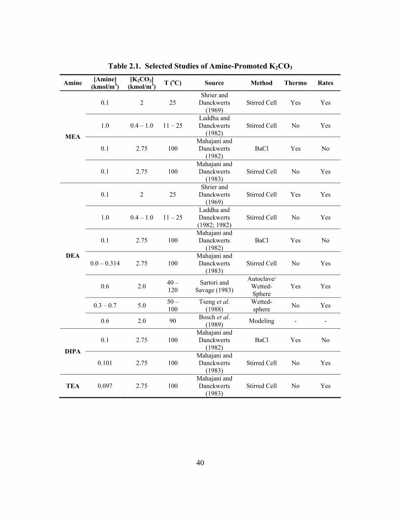
40
Table 2.1. Selected Studies of Amine-Promoted K2CO3
Amine [Amine] (kmol/m3)
[K2CO3] (kmol/m3) T (oC) Source Method Thermo Rates
0.1 2 25 Shrier and
Danckwerts (1969)
Stirred Cell Yes Yes
1.0 0.4 � 1.0 11 � 25 Laddha and Danckwerts
(1982) Stirred Cell No Yes
0.1 2.75 100 Mahajani and Danckwerts
(1982) BaCl Yes No
MEA
0.1 2.75 100 Mahajani and Danckwerts
(1983) Stirred Cell No Yes
0.1 2 25 Shrier and
Danckwerts (1969)
Stirred Cell Yes Yes
1.0 0.4 � 1.0 11 � 25 Laddha and Danckwerts (1982; 1982)
Stirred Cell No Yes
0.1 2.75 100 Mahajani and Danckwerts
(1982) BaCl Yes No
0.0 � 0.314 2.75 100 Mahajani and Danckwerts
(1983) Stirred Cell No Yes
0.6 2.0 40 � 120
Sartori and Savage (1983)
Autoclave/ Wetted-Sphere
Yes Yes
0.3 � 0.7 5.0 50 � 100
Tseng et al. (1988)
Wetted-sphere No Yes
DEA
0.6 2.0 90 Bosch et al. (1989) Modeling - -
0.1 2.75 100 Mahajani and Danckwerts
(1982) BaCl Yes No
DIPA
0.101 2.75 100 Mahajani and Danckwerts
(1983) Stirred Cell No Yes
TEA 0.097 2.75 100 Mahajani and Danckwerts
(1983) Stirred Cell No Yes
41
An investigation of carbamate equilibrium in hot potassium carbonate was
initiated by Mahajani and Danckwerts (1982). The study reports equilibrium constants
at 100oC for four amines, MEA; DEA; DIPA; and AMPD, as determined by rapid
mixing with barium chloride. The stability of carbamate decreased as MEA > AMPD >
DEA > DIPA, leading the authors to conclude that steric effects are responsible for
determining equilibrium.
Mahajani and Danckwerts (1983) also measured the effect of amines on the
desorption rates of CO2 from potash at stripper conditions (100oC). Amines chosen for
comparison in this study include DEA, MEA, DIPA, and AMP. The authors find that
DEA is a better promoter for the CO2 desorption than the others. This is due to the
equilibrium of DEA in comparison to the carbonate buffer. They also conclude that
absorption should also be enhanced, if the driving force is reversed.
A study of amine promoters of K2CO3 was published by Sartori and Savage
(1983) with an emphasis on hindered amines. Equilibrium and absorption rates are
reported for DEA and an unspecified hindered amine. The major conclusions from this
work are that the capacity and the absorption rate are increased by hindered amines due
to steric hindrance. The low carbamate stability increases the formation of the
bicarbonate and maintains a high concentration of free amine in solution.
Savage et al. (1984) investigated the VLE and rate behavior in DEA- and
hindered amine-promoted K2CO3. Results indicate that the promoters increase the rate
by a factor of 5 to 10 in K2CO3. The authors attribute the large promotion effect to the
amine serving as a homogeneous catalyst for CO2 hydrolysis.

42
Tseng et al. (1988) modeled the absorption rate of CO2 by 2 and 5 wt% DEA in
30 wt% K2CO3. Equilibrium behavior was represented by data from previous work.
Rate constants for the amine, hydroxide, and carbonate were regressed and activation
energies were determined. The authors observe a changing reaction order that is
accounted for in the interpretation of the �zwitterion� mechanism; however, a
discontinuity of rate constants suggests the behavior is not accurately represented.
Pohorecki et al. (1988) report findings on 0.05 to 0.20 M EAE in 1.5 M K2CO3
and present several important findings, including the support of earlier findings that the
rate is dependent on CO32- content. Some experiments were run in the presence of
neutral salts to buffer the ionic strength. In contrast to the previous work by Laddha
and Danckwerts (1982), it is proposed that ionic strength, not concentration of the
carbonate ion, is largely responsible for the increased absorption rates. The work does
not rigorously account for speciation of the amine, so it is difficult to distinguish
between equilibrium and kinetic effects. Still, the authors recognize the potential
importance of both ionic strength and carbonate concentration on the rate.
Kumar et al. (2003) measured the rate of absorption in amino acid-promoted
K2CO3 in a stirred cell. The reaction order of taurine and glycine is reported to increase
from 1 at concentrations greater than 1.0 M K+. The work concludes that either the
�zwitterion� or termolecular mechanism adequately represents the observed behavior.
43
2.3. Contributions to Reaction Kinetics
2.3.1. Acid and Base Catalysis
A major contribution to kinetic theory and physical chemistry was the
development of the theory of homogeneous catalysis by acids and bases. Much of the
original work in this area was done by Brønsted (1928). This work laid the foundation
for interpreting reaction mechanisms in terms of acid/base concentrations and provided
an important link between equilibrium strength and reaction rates. This section briefly
reviews some of the critical work in this area and relates them to the reaction of CO2
with amines.
The Brønsted theory defines a base as a molecule tending to unite with a
hydrogen nucleus and an acid as a molecule tending to split from a hydrogen nucleus.
Thus, in general, an equilibrium can be defined so that
KA A H− +→ +← , (2.39)
where A is the acid and A- is the corresponding base. Because in any solution the
concentration of hydrogen ion is small, it is more physically meaningful to describe the
above reaction relative to the hydronium equilibrium.
3 2wK
H O H O H+ +→ +← (2.40)
So, most reactions are represented as
2 3aK
A H O A H O− +→+ +← , (2.41)
where Ka = K/Kw. Ka is representative of the strength of the acid (or base) and is
usually written as
44
10loga apK K= − . (2.42)
Early work in physical chemistry indicated that many reactions depend
proportionally on the concentration of hydronium or hydroxyl ions in solution.
Brønsted held that the properties of these ions as acids and bases are not unique and the
catalytic effect on reactions should extend to other molecules. To date, a large body of
work has been performed corroborating and expounding on this theory.
One of the first efforts to distinguish the acid/base catalysis theory was a study
of the mutarotation of glucose (Brønsted and Guggenheim, 1927). This paper includes
a study of pyridine, a cyclic amine, and correlates the reaction rate of glucose with the
base strength. Conclusions of the theory were summarized by Livingston (1930):
1) Any acid or base may act as a catalyst.
2) The concentration of protons in any solution is small enough that the
catalytic effect is negligible.
3) The rate constant associated with the catalyst is different for each acid
or base and is different for each reaction.
Brønsted (1928) also found that the catalytic effect of bases on reaction rates can
be given as function of the base strength (i.e. dissociation constant). So, for a simple
reaction of the form
11
bkA b Prod+ → , (2.43)
where b1 is the catalyzing base, the following expression applies.
1 110 ,log b a bk x pKχ= + (2.44)

45
where χ and x are reaction-specific constants and pKa,b1 represents the base strength.
A study of the decomposition of nitramide demonstrated that amines are
effective as base catalysts and can be represented in this general form (Bell and
Trotman-Dickenson, 1949; Trotman-Dickenson, 1949). In addition, it was determined
that the rate constant for the reaction could be correlated by four distinguishable classes
of amines: primary, secondary, tertiary, and heterocyclic. Sharma (1965) summarized
the rate constants of numerous amines reacting with CO2 and demonstrated that a
correlation with base strength applies. Other researchers in the area have shown similar
correlating behavior (Littel et al., 1992a; Rochelle et al., 2001).
Though base catalysis has been widely recognized as a contributing factor in the
kinetics of amines reacting with CO2, this reaction involves two bases: the amine, Am,
reacts with the CO2 and the base, b1, catalyzes the reaction.
12 1 1
Am bkCO Am b AmCOO H b− − ++ + → + (2.45)
Following the sequence of reaction according to the proposed mechanism (Equations
(2.26) and (2.27)), there are two correlations with base strength. The termolecular
reaction rate can be expressed as a product of the two correlations (Equation (2.30)).
( )( )1 1 ,, 1
1 110 10 a bAm Am a Am a b pKa b pKf
Am b Am br
kk k
k++
− −= = (2.46)
Thus,
( ) ( )1 1 1 110 , ,log Am b Am Am a Am b b a bk a b pK a b pK− = + + + . (2.47)
46
Since the amine-CO2 interaction can be assumed constant, the contribution of unknown
bases in this complex reaction may still be correlated by the difference in base strength.
( )2 1 2 110 10 , ,log logAm b Am b a b a bk k pK pKχ− −= + − (2.48)
From the previous efforts in this field and the proven validity of Brønsted theory
as applied to the capture of CO2, the kinetic mechanism proposed in this work can
justifiably rely in a large part on the correlation of kinetics to base strength.
2.3.2. Neutral Salt Effects
During a reaction between two or more molecules, the molecules come together
in a configuration of high potential energy relative to that of the reactants and products.
The molecules pass through this transition state as the reaction proceeds to the products.
The resulting theory can be written generically so that a bi-molecular reaction occurs as
( )( ) *K k ProductsA B
A Bz z
z zA B AB+∗→+ →← , (2.49)
where (AB)* represents the transition state, or a reaction intermediate, and z is the
charge of the species. An important corollary of this theory is that the reactants and
transition state are considered to be in equilibrium. For this reaction, an equilibrium
constant is written in the form
( )[ ][ ]
( )*
*
AB
A B
ABK
A B
γ
γ γ
= . (2.50)
The rate of consumption of the intermediate is considered to be
( )**r k AB = . (2.51)
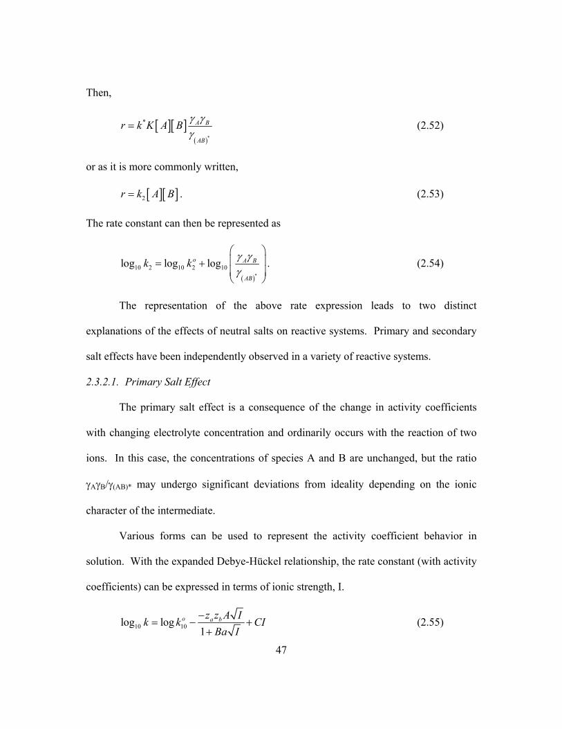
47
Then,
[ ][ ]( )*
* A B
AB
r k K A B γ γγ
= (2.52)
or as it is more commonly written,
[ ][ ]2r k A B= . (2.53)
The rate constant can then be represented as
( )*10 2 10 2 10log log logo A B
AB
k k γ γγ
= +
. (2.54)
The representation of the above rate expression leads to two distinct
explanations of the effects of neutral salts on reactive systems. Primary and secondary
salt effects have been independently observed in a variety of reactive systems.
2.3.2.1. Primary Salt Effect
The primary salt effect is a consequence of the change in activity coefficients
with changing electrolyte concentration and ordinarily occurs with the reaction of two
ions. In this case, the concentrations of species A and B are unchanged, but the ratio
γAγB/γ(AB)* may undergo significant deviations from ideality depending on the ionic
character of the intermediate.
Various forms can be used to represent the activity coefficient behavior in
solution. With the expanded Debye-Hückel relationship, the rate constant (with activity
coefficients) can be expressed in terms of ionic strength, I.
10 10log log1
o a bz z A Ik k CIBa I
−= − +
+ (2.55)
48
A, B, and C are ion specific constants and a is the ion size parameter. In concentrated
salt solutions, the expression is often dominated by the linear term CI. Thus, a
simplification can be made in which log k is proportional to the ionic strength.
10 10log logk k CI∞= + (2.56)
This phenomenon has been observed in numerous systems. Much of the early
work in this area was performed by Brønsted in his development of theory. Brønsted
and Teeter (1924) quantified a primary salt effect in the reaction of mercuric nitrate
with chloropentammine cobaltic nitrate. The two positively-charged reactants show a
distinct increase in reaction rate with additional ionic strength. Other ionic reactions
demonstrate similar behavior (Olson and Simonson, 1949).
2.3.2.2. Secondary Salt Effect
A secondary salt effect may alter the reaction rate by changing the
concentrations of A and B while the activity coefficient ratio remains constant
(Brønsted and Teeter, 1924). This is usually associated with enhancing the dissociation
of the reactive ions through the addition of neutral salts, though the effect has been
observed in reactions of neutral species. Thus, the important distinction here is that the
effect is not a kinetic effect per se, but rather a change in �inter-ionic forces� (Brønsted
and King, 1925).
One study, particularly useful for demonstrating the secondary salt effect,
quantifies the effect of neutral salts on the decomposition of nitroso-triacetone-amine
where hydroxyl ion is an active catalyst (Brønsted and King, 1925). In the presence of
a piperidine buffer, whose equilibrium can be written

49
5 11 2 5 12C H N H O C H N OH+ −→+ +← , (2.57)
the effect of neutral salts is verified to increase the reaction velocity by increasing the
hydroxyl concentration. The salts increase the stability of the ions in solution and move
the above equilibrium to the right. An 18% increase in the apparent rate constant is
observed with the addition of 0.2 N NaCl. In the presence of a phosphate buffer, where
3 24 2 4PO H O HPO OH− − −→+ +← , (2.58)
the stability of the lesser charge distribution pushes the equilibrium to the left in the
presence of neutral salts. A negative salt effect (a reduction of the catalytic species,
OH-) is expected and observed. The apparent rate constant is 42% lower in 0.2 N NaCl.
2.3.2.3. Combinatorial Effects
Many of the initial investigations into the neutral salt effect rely on carefully
designed experiments to isolate the primary or secondary mechanism for study. In this
regard, the investigations represent highly idealized work. In more complicated, and
non-ideal, systems, both primary and secondary salt effects may play a significant role
in determining the reaction rate. Some studies have been performed on systems with no
attempt to isolate either the primary or secondary salt effect, and represent the overall
impact of neutral salt addition on reactions.
French (1928) studied the iodine-catalyzed decomposition of hydrogen
peroxide. The influence of up to 2 M of several neutral salts increased reaction rates by
as much as a factor of two. Grube and Schmid (1926) measured the effect of
50
concentrated neutral salts on the hydrolysis of cyanamide. The authors again find the
reaction rates in 2 M ionic strength increase by a factor of two.
Neutral salts have also been shown to positively influence the absorption rate of
CO2 into amines. Data from Danckwerts and Sharma (1966) and Laddha and
Danckwerts (1982) suggest a significant promotion effect due to ionic strength.
Given the high ionic strengths encountered in this work, salt effects are expected
to play a significant role in determining the rate of CO2 absorption. Pohorecki et al.
(1988) and Kloosterman et al. (1987) documented this effect in potassium carbonate
systems and applied a correction for ionic strength to the rate constant. It is no doubt a
factor in all work with promoted K2CO3, though it is rarely recognized and never
quantified.
51
Equation Chapter 3 Section 1
Chapter 3: Experimental Methods
This chapter outlines the experimental methods and apparatuses used in this
work for quantifying the behavior of K+/PZ mixtures, including discussions on data
analysis and limitations. A wetted-wall column was used to measure the equilibrium
partial pressure of CO2 and the rate of CO2 absorption. Nuclear magnetic resonance
spectroscopy was used to measure PZ speciation in the presence of CO2. Measurements
of density, viscosity, physical CO2 solubility, and solid solubility were also performed.
The methods for determining these properties are presented.
3.1. Wetted-Wall Column
A wetted-wall column was used for all vapor-liquid equilibrium and CO2
absorption rate experiments in this work. The apparatus was originally built by
Mshewa (1995) and has been used in several recent investigations including Pacheco
(1998), Bishnoi (2000), Dang (2001), and Cullinane (2002).

52
3.1.1. Equipment Description
The wetted-wall column, shown in Figure 3.1, consists of a stainless steel tube
9.1 cm long with a 1.26 cm outer diameter. The total contact area, 38.52 cm2, is
calculated as the longitudinal area of the tube, 36.03 cm2, and the area of the top of the
column (considered a hemisphere due to the shape of liquid film), 2.49 cm2. The
column is enclosed by a thick-walled glass cylinder with an outside diameter of 2.54 cm
to provide the gas-liquid contact chamber. The hydraulic diameter (outer diameter
minus inner diameter) of the enclosure is 0.44 cm, giving a cross-sectional area for gas
flow of 1.30 cm2. The chamber is housed inside a second thick-walled glass cylinder
(10.16 cm OD) that serves as an insulating bath with circulating heat transfer fluid.
9.1 cm
1.26 cm
2.54 cm
10.16 cm
T
T
P
Liquid Out
Liquid In
Gas In ParaffinOil Inlet
ParaffinOil Outlet
Gas Out
9.1 cm
1.26 cm
2.54 cm
10.16 cm
T
T
P
Liquid Out
Liquid In
Gas In ParaffinOil Inlet
ParaffinOil Outlet
Gas Out
Figure 3.1. Diagram of the Wetted-Wall Column Construction

53
A representation of the full experimental setup is shown in Figure 3.2. The
liquid solution was contained in a reservoir (a series of modified calorimetric bombs)
with a total volume of 1,400 cm3. The fluid was pushed from the reservoir to the gas-
liquid contact chamber. The fluid flowed up through the middle of the column,
overflowed at the top, and evenly distributed on the outer surface of the column. The
liquid was collected at the bottom of the column and pumped back to the solution
reservoir. A liquid rotameter indicated the volumetric flowrate of the liquid. It was
calibrated with water, giving the following equations:
( )3, 0.4512x - 0.2901
refw TQ cm s = , (3.1)
( )3, ,
(7.83- )
(7.83- 0.997)ref
ref ref
ref
Tsol T w T
T
Q cm s Qρ
ρ= , (3.2)
and
( )2
3, 2
7.837.83ref
ref
sol sol TT
Q cm s Q ρρ
−=
−, (3.3)
where Qw is the volumetric flowrate of water, Qsol is the volumetric flowrate of the
solution, ρ is the density of the solution in g/cm3, and x is the rotameter reading. The
value of 7.83 represents the density of the rotameter float. The subscript Tref refers to
the value at a standard temperature of 25oC. The liquid temperature was measured at
the inlet and outlet of the contactor by Type-J thermocouples (± 2.2oC).
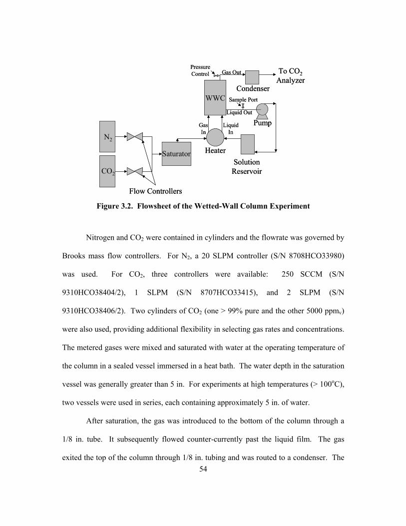
54
WWC
N2
CO2
Flow Controllers
Saturator HeaterSolution
Reservoir
Gas Out
GasIn
LiquidIn
Liquid Out
Condenser
To CO2Analyzer
Sample Port
PressureControl
Pump
WWC
N2
CO2
Flow Controllers
Saturator HeaterSolution
Reservoir
Gas Out
GasIn
LiquidIn
Liquid Out
Condenser
To CO2Analyzer
Sample Port
PressureControl
Pump
Figure 3.2. Flowsheet of the Wetted-Wall Column Experiment
Nitrogen and CO2 were contained in cylinders and the flowrate was governed by
Brooks mass flow controllers. For N2, a 20 SLPM controller (S/N 8708HCO33980)
was used. For CO2, three controllers were available: 250 SCCM (S/N
9310HCO38404/2), 1 SLPM (S/N 8707HCO33415), and 2 SLPM (S/N
9310HCO38406/2). Two cylinders of CO2 (one > 99% pure and the other 5000 ppmv)
were also used, providing additional flexibility in selecting gas rates and concentrations.
The metered gases were mixed and saturated with water at the operating temperature of
the column in a sealed vessel immersed in a heat bath. The water depth in the saturation
vessel was generally greater than 5 in. For experiments at high temperatures (> 100oC),
two vessels were used in series, each containing approximately 5 in. of water.
After saturation, the gas was introduced to the bottom of the column through a
1/8 in. tube. It subsequently flowed counter-currently past the liquid film. The gas
exited the top of the column through 1/8 in. tubing and was routed to a condenser. The
55
condenser was constructed from a 1 L Erlenmeyer flask submerged in an ice bath. The
gas entered and exited at the top of the condenser while the condensing water was
allowed to settle at the bottom of the flask. Much of the gas was vented from a valve on
the condenser to reduce load on downstream components. Approximately 1 L/min of
the gas was sent to a drying column containing magnesium perchlorate to remove
excess moisture. The dry gas was then sent to a gas analyzer for composition
determination. Pressure in the column was controlled by a needle valve on the gas
outlet tubing. An analog pressure gauge (Matheson, P/N 63-3122) was used to monitor
pressures between 35 and 55 psig (± 2 psig).
3.1.2. Gas Analysis
The concentration of CO2 in the outlet gas was measured by Horiba PIR-2000
gas analyzers. The available range of the analyzers was adjustable, varying from 0.05
to 25 vol%, with an expected accuracy of 0.1% of full scale. The equipment uses IR
spectroscopy to measure the amount of CO2 in the gas phase. The analyzers were
calibrated prior to each experiment by bypassing the wetted-wall column and adjusting
the CO2 flowrate in the feed gas to give known concentrations. A chart recorder was
used during the calibrations and experiments to record the response of the analyzers.
Readings from the recorder are expected to be accurate to 0.2% of full scale.
3.1.3. Liquid Analysis
During each experiment, liquid samples were taken from the wetted-wall
column so that a liquid CO2 concentration could be determined. The samples were
withdrawn from a septum on the liquid outlet tubing by a 150 µL syringe. The samples
56
were diluted; generally, 100 µL of sample was placed in 5 mL DI H2O. For analysis,
the diluted samples were injected into 30 wt% H3PO4 sparged with nitrogen. The acid
liberated all inorganic carbon from the solution and the nitrogen sweep gas (~ 0.5
L/min) carried the gas phase to the Horiba PIR-2000 gas analyzer (range 0.05 vol%).
The gas stream was passed through a drying column of magnesium perchlorate prior to
entering the analyzers.
This method was calibrated prior to each use by injecting several known
volumes of 7 mM Na2CO3. Generally, volumes of 50, 100, 150, and 200 µL were used
to obtain a calibration curve for the analyzer response. During the calibration and the
experiments, the response was recorded on a chart recorder. Because sharp peaks are
obtained, the peak height, and not peak area, was assumed to be representative of the
CO2 concentration.
3.1.4. Physical Mass Transfer Coefficients
3.1.4.1. Gas Film Mass Transfer Coefficient
The gas film mass transfer coefficient, kg, in the wetted-wall column was
determined by Bishnoi (2000) using SO2 absorption into 0.1 M NaOH. The results of
these experiments are correlated with a form for kg proposed by Hobler (1966).
0.85
1.075 dSh ReSch
=
(3.4)
The Reynolds number is defined as
u dRe ρµ
= , (3.5)

57
where u is the linear velocity of the gas, ρ is the density, and µ is the viscosity. Also, d
is the hydraulic diameter of the annulus (0.44 cm) and h is the height of the wetted-wall
column (9.1 cm). The Schmidt number is
2CO
ScDµ
ρ= . (3.6)
DCO2 is the diffusion coefficient of CO2. The gas film transfer coefficient can be found
from the following definition of the Sherwood number.
2
g
CO
RTk hSh
D= (3.7)
where T is the temperature and R is the gas constant.
Experiments in the wetted-wall column were run with high gas rates (5 to 7
L/min) to minimize the gas film resistance to mass transfer. Most data points had 20 to
50% gas film resistance. Figure 3.3 shows kg as a function of gas flowrates.
3.1.4.2. Liquid Film Mass Transfer Coefficient
Mshewa (1995) and Pacheco (1998) determined the liquid film mass transfer
coefficient, klo, of the wetted-wall column by CO2 desorption from water and ethylene
glycol. Mshewa originally used a theoretical prediction of klo based on work from
Vivian and Peaceman (1956). Pacheco determined that additional data and an expanded
correlation were needed to accommodate varying experimental conditions. This
correlation was developed from falling-film theory developed by Pigford (1941) using a
momentum balance as presented by Bird et al. (1960).
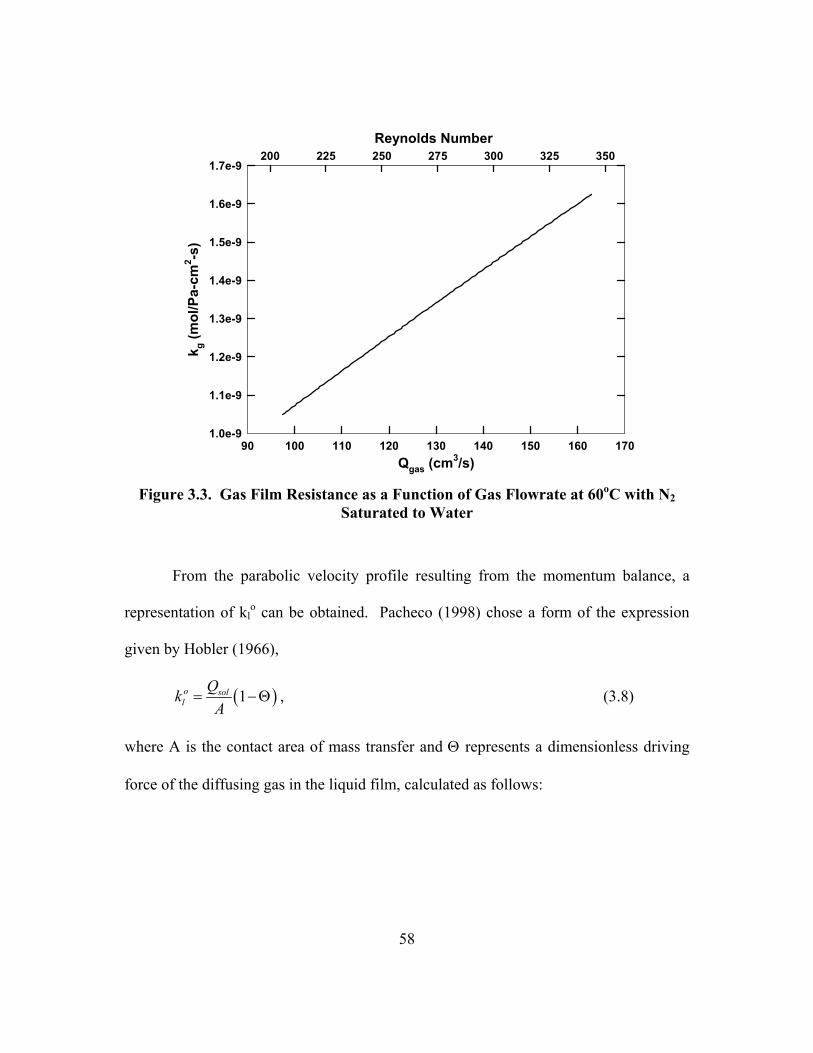
58
Qgas (cm3/s)90 100 110 120 130 140 150 160 170
k g (m
ol/P
a-cm
2 -s)
1.0e-9
1.1e-9
1.2e-9
1.3e-9
1.4e-9
1.5e-9
1.6e-9
1.7e-9
Reynolds Number200 225 250 275 300 325 350
Figure 3.3. Gas Film Resistance as a Function of Gas Flowrate at 60oC with N2
Saturated to Water
From the parabolic velocity profile resulting from the momentum balance, a
representation of klo can be obtained. Pacheco (1998) chose a form of the expression
given by Hobler (1966),
( )1o soll
QkA
= − Θ , (3.8)
where A is the contact area of mass transfer and Θ represents a dimensionless driving
force of the diffusing gas in the liquid film, calculated as follows:
59
[ ] [ ][ ] [ ]
( ) ( )
( ) ( )
2 2
2 2
0.7857 exp 5.121 0.1001exp 39.21
0.036exp 105.6 0.0181exp 204.7 , for 0.01
out
i oin
i o
CO CO
CO COη η
η η η
−Θ = = − + − +
−
− + − >
,
(3.9)
or
1 3 , for 0.01η ηπ
Θ = − < , (3.10)
where [CO2]oin and [CO2]o
out represent the concentration of CO2 in the bulk liquid at the
inlet and outlet of the wetted-wall column, respectively, and [CO2]i is the concentration
of CO2 at the gas-liquid interface. η is a dimensionless penetration distance defined as
2
2COD τ
ηδ
= , (3.11)
and τ is the surface contact time, defined as
s
hu
τ = . (3.12)
The height of the wetted-wall column is represented by h.
The film thickness, δ, is given by
33 solQ
gWµδρ
= , (3.13)
where µ is the liquid viscosity, Q is the volumetric flowrate of the liquid, ρ is the liquid
density, g is the gravity constant, and W is the circumference of the column. A liquid
surface velocity, us, is given by
60
2
2sgu ρ δµ
= . (3.14)
Most experiments in the wetted-wall column were run so that klo was between 0.007
and 0.014 cm/s.
3.1.5. Interpretation of Experimental Measurements
Several data points were collected during each experiment at various bulk gas
partial pressures. The flux of CO2 into or out of the solution can be characterized by the
overall gas phase mass transfer coefficient.
( )*, 222 CObCOGCO PPKN −= (3.15)
The mass transfer coefficient, KG, is calculated as the slope of the flux versus the log
mean pressure, Plm. The Plm is defined as a log mean average of bulk gas partial
pressures of CO2 across the wetted-wall column and is assumed representative of PCO2,b.
( )2 2
2 2
, ,
, ,lnCO in CO out
lmCO in CO out
P PP
P P
−= (3.16)
The equilibrium partial pressure, PCO2*, can be found by considering points close to
equilibrium and interpolating to a flux of 0.0, a technique initiated by Critchfield
(1988). A demonstration of this procedure is shown in Figure 3.4.
An expression of the liquid film resistance, which includes the kinetics of CO2
absorption, can be written as
( )*, 222
' COiCOgCO PPkN −= , (3.17)
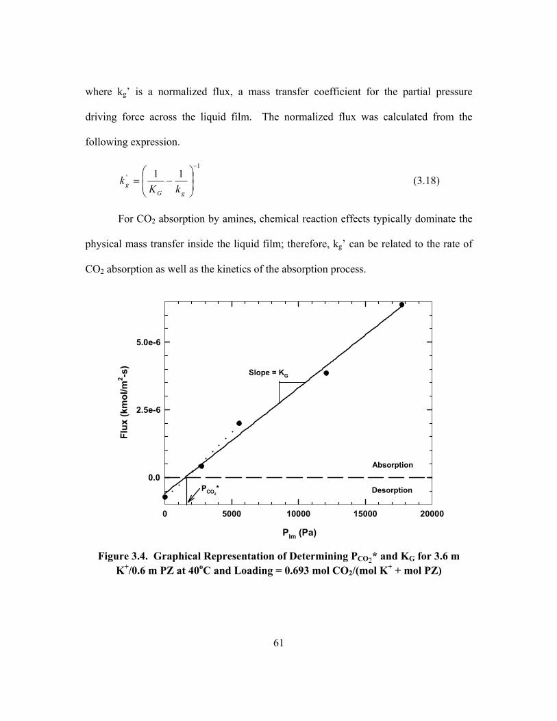
61
where kg� is a normalized flux, a mass transfer coefficient for the partial pressure
driving force across the liquid film. The normalized flux was calculated from the
following expression.
1
' 11−
−=
gGg kK
k (3.18)
For CO2 absorption by amines, chemical reaction effects typically dominate the
physical mass transfer inside the liquid film; therefore, kg� can be related to the rate of
CO2 absorption as well as the kinetics of the absorption process.
Plm (Pa)
0 5000 10000 15000 20000
Flux
(km
ol/m
2 -s)
0.0
2.5e-6
5.0e-6
Absorption
Desorption
Slope = KG
PCO2*
Figure 3.4. Graphical Representation of Determining PCO2* and KG for 3.6 m
K+/0.6 m PZ at 40oC and Loading = 0.693 mol CO2/(mol K+ + mol PZ)
62
3.2. Nuclear Magnetic Resonance Spectroscopy
Proton nuclear magnetic resonance (1H NMR) spectroscopy was used to
determine the equilibrium distribution of piperazine species in the liquid phase. A
Varion INOVA 500 NMR was used for the measurements. The machine has a field
strength of 500 MHz and is capable of variable temperature work.
Samples were made with K2CO3, KHCO3, PZ and water. Approximately 20%
of the water was replaced with D2O (heavy water). One drop of 2,2-dimethyl-2-
silapentane-5-sulfonic acid (DSS) in D2O was added to each sample to maintain a
constant chemical shift reference. After all components were dissolved with mild
heating, the samples were placed in Wilmad 507-PP NMR tubes. A slight vacuum was
applied and the tube was permanently sealed by a simple glass blowing technique.
Bishnoi (2000) assigned the proton peaks for PZ based on their correlation to the
carbon-13 spectrum. The chemical shifts vary somewhat with loading and solvent
conditions, but the distinctiveness of the peaks allows easy identification based solely
on the 1H spectrum. A typical spectrum is shown in Figure 3.5. The PZ/PZH+ and
PZ(COO-)2 peaks show up as single peaks near 2.9 and 3.2 ppm respectively. PZCOO-
and H+PZCOO- are represented by two triplet peaks centered near 2.8 and 3.3; the sum
of the two triplets gives the total carbamate concentration.

63
Figure 3.5. Proton NMR Spectrum of 3.6 m K+/0.6 m PZ, Loading = 0.630 mol
CO2/(mol K+ + mol PZ), 27oC
One major limitation of 1H NMR as applied in this work is its inability to
distinguish between some chemical species that are in equilibrium. This is related to
the field strength of the machine and the velocity of the equilibrium exchange. For
example, the 500 MHz machine used in this work has an inherent time scale of 2x10⁹ s
(1/500 MHz). Any two species whose equilibrium occurs at a faster rate will be
indistinguishable. Therefore, in this work, protonated and un-protonated forms of PZ
can not be measured independently; all peaks, in this case, represent the sum of the two
species. This condition also imposes a temperature limit. At temperatures near 60oC,
the velocities of the carbamate equilibria become sufficiently fast as to blur previously

64
well-defined peaks. Compare Figure 3.5 and Figure 3.6, the same solution measured at
27 and 60oC, for a demonstration of peak broadening. In some cases, the severity of the
peak broadening renders the measurement useless for quantitative interpretations.
Nearly all data points collected in this work are at or below 60oC.
Figure 3.6. Proton NMR Spectrum of 3.6 m K+/0.6 m PZ, Loading = 0.630 mol
CO2/(mol K+ + mol PZ), 60oC
3.3. Solid Solubility
Both piperazine and potassium carbonate are solids at their standard state
conditions. Because the imposition of solid solubility restricts the total solvent
concentration, quantification of the limits are required to identify viable commercial
65
solvent formulations and provide additional thermodynamic information for
concentrated mixtures.
Approximately 100 g of concentrated K+ and PZ was prepared so that a
precipitate would form. The solutions were immersed in a constant temperature bath
and stirred with a magnetic stir plate for at least 12 hours to ensure solid-liquid
equilibrium. Once equilibrium was achieved, a 10 mL sample of the saturated liquid
was removed by pipette and placed in a beaker. The sample was titrated with 2 N HCl
to an endpoint indicated by methyl orange pH indicator (range 3.0 to 4.4). The solution
was then briefly boiled, driving off dissolved CO2. A base titration was done, using 2 N
NaOH, to an endpoint of -265 mV as indicated by a pH meter. This voltage reading
was found to correspond roughly to the endpoint of pH 11 in the concentrated solutions.
The acid titration gives the total alkalinity of the sample. The base titration
gives the equivalents of PZ in solution. (CO2 was boiled off so that no bicarbonate or
carbonate formed during the base titration.) So, the resulting calculations may be made
for a sample of fixed volume.
2 mol acid mol K mol PZ+= + ⋅ (3.19)
2 mol base mol PZ= ⋅ (3.20)
A small liquid sample was collected and analyzed for loading as described previously in
Section 3.1.3.
66
3.4. Physical Properties
3.4.1. Density
The density of K+/PZ mixtures was measured with a Mettler/Paar #DMA46
Digital Density meter. The measurement is based on the principle that a resonating
frequency in an object is inversely proportional to the square root of mass.
1fm
∝ (3.21)
A fixed volume of solution is injected into the apparatus and a frequency of vibration is
measured. From the estimated mass, the density is calculated.
The instrument was calibrated with air and water, giving constants for the
density calculation of the form
2 2water air
water air
T Taρ ρ
−=
−, (3.22)
and
2water waterb T aρ= − , (3.23)
where T is the measured period of oscillation. Density of the unknown is calculated as
2T ba
ρ −= . (3.24)
Densities of aqueous K+/PZ mixtures were measured at 25 and 40oC. Density is
reported to ± 0.001 g/cm3. The results of the experiments are recorded in Appendix A.
It was determined that the amine had little effect on density over the range of soluble
concentrations; this effect has also been observed with other amines (Weiland et al.,
67
1998). A small dependence on temperature and loading was also observed, but the
main contribution to density was the salt concentration (K2CO3/KHCO3). The
measured density compares well with the measurements of K2CO3 solutions by
Hitchcock and McIlhenny (1935).
An empirical representation of density was derived for use in calculations. The
expression was used in all calculations involving density in this work. Model
predictions are compared to the experimental data in the previous tables.
[ ]23 33
3 3
1.130 0.0537 1.204 10 1.882 10
0.442 10 9.010 10
g K K PZcm
T
ρ
α
+ − + −
− −
= + − × + × − × + ×
(3.25)
where [i] is the concentration of species i in molal, T is temperature in Kelvin, and α is
the loading in mol CO2/(mol K+ + mol PZ).
3.4.2. Viscosity
An extensive collection of data exists quantifying the viscosity of aqueous
electrolyte solutions, including K2CO3 (Bates and Baxter, 1929; Hitchcock and
McIlhenny, 1935; Bocard and Mayland, 1962; Goncalves and Kestin, 1981; Moniuk
and Pohorecki, 1991; Vazquez et al., 1994). The data sets include a wide variety of
conditions (0 to 7.5 m K2CO3 and 0 to 2.0 m KHCO3 at 20 to 60oC).
Though data are available, correlating the viscosity of electrolyte solutions can
be considerably difficult as fluid properties vary widely with composition and
temperature. Some authors use complex group contribution methods or matrix
68
calculations to express density. The most convenient method of correlating viscosity,
however, is by an empirical expression. The simplest form representing the data is
[ ]1ln ln w C Saltµ µ= + , (3.26)
where µ represents the dynamic viscosity in the mixture, µw is the dynamic viscosity of
water, and C1 is a constant for specific salts (Moniuk and Pohorecki, 1991; Vazquez et
al., 1994).
The viscosity of aqueous organic mixtures has also been studied in detail. Cook
and Lowe (1976) report the viscosity of aqueous PZ in dilute solutions (< 0.2 m PZ) and
represent the data in the following empirical form.
[ ] [ ]21 2w C Am C Amµ µ= + + (3.27)
No studies of aqueous electrolyte-organic mixtures could be found in the
literature; therefore, the viscosity of K+/PZ mixtures at conditions encountered in this
work was measured in a routine Cannon-Fenske viscometer (Cannon Instrument Co.,
No. 100, 3�15 cSt). The measurements are based on fluid flow through a capillary tube,
which is directly related to fluid viscosity.
A representation of the viscometer is shown in Figure 3.7. The viscometer was
placed in a water bath to maintain the desired temperature. A sample of a set volume
was placed in section A. The fluid was drawn up to point B in the viscometer by a
suction bulb. The time of the meniscus moving from point B to C was measured by a
stopwatch.

69
B
A
C
CapillarySection
Figure 3.7. Cannon-Fenske Viscometer
Viscosity, in mPa-s (or cP), is related to time by
tµ βρ= , (3.28)
where β is the viscometer constant determined through calibrations in cSt/s (or mm2/s2),
ρ is the solution density in g/cm3, and t is the measured time in seconds. The
instrument was calibrated with water at 25, 40, 60 and 70oC. A constant solution
volume of 7 mL was used during calibration and measurement.
The results of the viscosity experiments are given in Appendix A. An empirical
representation, based on a combination of the expressions for aqueous salts and aqueous
PZ, was derived from the data. The regressed constants are reported in Table 3.1.
( ) [ ] [ ]( )[ ]
[ ]
021 2 / /exp
1
A E T G Tw B K C De PZ Fe PZ
K PZH K PZ I
T
µ µ α+ +
++
= + + + ×
+ +
(3.29)
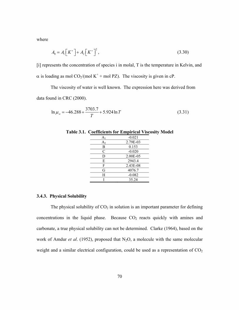
70
where
2
0 1 2A A K A K+ + = + , (3.30)
[i] represents the concentration of species i in molal, T is the temperature in Kelvin, and
α is loading as mol CO2/(mol K+ + mol PZ). The viscosity is given in cP.
The viscosity of water is well known. The expression here was derived from
data found in CRC (2000).
3703.7ln 46.288 5.924lnw TT
µ = − + + (3.31)
Table 3.1. Coefficients for Empirical Viscosity Model
A1 -0.021 A2 2.79E-03 B 0.153 C -0.020 D 2.00E-05 E 2943.4 F 2.43E-08 G 4076.7 H -0.082 I 35.24
3.4.3. Physical Solubility
The physical solubility of CO2 in solution is an important parameter for defining
concentrations in the liquid phase. Because CO2 reacts quickly with amines and
carbonate, a true physical solubility can not be determined. Clarke (1964), based on the
work of Amdur et al. (1952), proposed that N2O, a molecule with the same molecular
weight and a similar electrical configuration, could be used as a representation of CO2
71
behavior in reactive systems. The assumption for the N2O analogy is that the ratio of
CO2 to N2O solubility is constant for all systems.
2
2
constantCO
N O
HH
= (3.32)
Given this relation, the solubility of N2O can be measured in amine solutions and a
solubility of CO2 can be approximated by relating the ratio to that in water. That is
2
2 2
2
,, ,
,
CO wCO Am N O Am
N O w
HH H
H
=
. (3.33)
The Henry�s constants for CO2 and N2O in water were correlated by Versteeg and van
Swaaij (1988b).
( )2
4,
20443.54 10 expCO wmolH
L Pa T K− = × ⋅
(3.34)
( )2
4,
22841.17 10 expN O wmolH
L Pa T K− = × ⋅
(3.35)
The physical solubility of N2O in K+/PZ mixtures was determined using the
apparatus depicted in Figure 3.8. The apparatus was built by Al-Jauied (2004) and is
similar to that used in the work of Al-Ghawas (1989) to determine the physical
solubility of N2O in amines. The apparatus consisted of a sample cell (~250 mL), a gas
washing bottle, a manometer, and a mercury reservoir of adjustable height. The entire
apparatus, except for the mercury reservoir, was immersed in a constant temperature
bath.

72
N2O
Stir Plate Water Bath
Block Valve 1
Block Valve 2
Hg Manometer
Hg Reservoir
Septum
Saturator
N2O
Stir Plate Water Bath
Block Valve 1
Block Valve 2
Hg Manometer
Hg Reservoir
Septum
Saturator
Figure 3.8. Apparatus for Physical Solubility Measurements
To measure the solubility of N2O in a sample, the empty sample cell was flushed
with N2O for approximately 20 minutes. The N2O gas was sparged through water in the
gas washing bottle, saturating the gas at the desired operating temperature prior to
entering the sample cell. The flow of N2O was stopped; block valves on the inlet and
outlet of the apparatus trapped the gas inside the sample cell.
A sample of known volume and mass was injected into the cell and the
corresponding volume change was monitored on the manometer. The sample was
degassed using a vacuum pump prior to injection. The height of the mercury reservoir
was adjusted to maintain atmospheric pressure inside the system. The solution was
stirred and allowed to equilibrate for approximately one hour. The volume change, as
73
indicated by the manometer, minus the volume of liquid injected gave the volume
(solubility) of N2O in the sample at equilibrium. The solubility of CO2 was calculated
using the analogy described previously.
3.4.4. Diffusion Coefficient
3.4.4.1. Diffusion of CO2
The diffusion coefficient of CO2 in solution was also estimated by the N2O
analogy. This method has been used previously in several studies on CO2 absorption by
amines and is similar to the analogy presented for physical solubility. The diffusivity of
CO2 and N2O in water were determined by Versteeg and van Swaaij (1988b) and
Tamimi et al. (1994a, 1994b). The data were correlated by Pacheco (1998) and are
given by the following expressions.
( ) ( )2
2,
2122.20.02397expCO wD cm sT K
−=
(3.36)
( ) ( )2
2,
2288.40.04041expN O wD cm sT K
−=
(3.37)
DN2O in amines was correlated to viscosity and temperature by Pacheco (1998).
( ) ( )( )2
2 8, 0.5455.533 10N O Am
T KD cm s
cPµ−= × (3.38)
The ratio of DCO2 to DN2O is assumed to be constant; therefore, the diffusivity of CO2 in
amine solutions is estimated by
2
2 2
2
,, ,
,
CO wCO Am N O Am
N O w
DD D
D= . (3.39)
74
3.4.4.2. Diffusion of Amines and Ions
For fast kinetics, the diffusion of the amine and products to and from the gas-
liquid interface may limit the overall reaction rate. Additionally, it defines, under high
fluxes, concentration gradients existing in the boundary layer. It is important, therefore,
to obtain an accurate prediction of the diffusion coefficient of the organic and ionic
components in aqueous solution.
In the simplest form, the diffusion of molecules can be described by the Stokes-
Einstein relation. It has been shown that, at infinite dilution, the diffusion coefficient of
the amine is related to the molar volume of the solute. A more sophisticated model, the
Wilke-Chang correlation (Wilke and Chang, 1955), was used in this work, giving the
diffusion coefficient as a function of solvent viscosity, temperature, and solvent specific
parameters.
( )0.513
0.6
1.17 10 sol solAm
Am sol
MW TD
Vξ
µ
−∞ ×
= (3.40)
where ∞ denotes the diffusion coefficient of the amine at infinite dilution in water, V
indicates molar volume, MWsol is the molecular weight of the solvent, and ξsol
represents the solvent specific parameter (2.6 for water).
The Wilke-Chang correlation predicts the diffusion coefficient of amines and
other organic molecules, such as carboxylic acids, to within 10% (Albery et al., 1967;
van der Wielen et al., 1997; Schramke et al., 1999). Predictions also match the
experimentally determined diffusion coefficient of piperidine, a six-membered ring
structure with only one nitrogen (Barradas et al., 1971). It is also reported that little
75
difference is realized in mobility between neutral, mono-, and di-valent ions; therefore,
the diffusivities of protonated species can be assumed to be equal to their un-protonated
counterparts (van der Wielen, 1997). Given the numerous sources verifying the ability
of Wilke-Chang to estimate the diffusion coefficient of organics, ions, and specifically
amines, it is assumed a reasonable estimate will be obtained for species in this work.
The diffusion coefficient of PZ was estimated using a molar volume of 0.1052
m3/kmol predicted from the group contribution method of Le Bas (1915). Because the
absorption rate model (Section 4.2) requires a charge balance, the diffusion coefficients
of all ions must be assumed equal. An average value for all ionic species was estimated
by setting all diffusion coefficients equal to that of PZCOO-. The molar volume of
PZCOO- is predicted to be 0.1311 m3/kmol (Le Bas, 1915). For comparison, the molar
volume of PZ(COO-)2 is 0.1570 m3/kmol. By assuming PZCOO- is representative of
the molar volume for all species, differences in AmD∞ of approximately 10% are expected
from the true value of PZH+ and PZ(COO-)2.
The extrapolation of D∞ to higher concentrations has been determined to be
dependent on the specific solute-solvent interaction. In general, the diffusion
coefficient of amines can be related to D∞ and viscosity by
0.6
wAm Am
Am
D D ηη
∞ =
(3.41)
(Campbell and Lam, 1973; Snijder et al., 1993; Hikita et al., 1981; Albery et al., 1967;
van der Wielen, 1997).
76
3.5. Chemicals and Materials
The potassium carbonate [584-08-7] and potassium bicarbonate [298-14-6] used
in this work were obtained from Fisher and were 100% and 99.9% pure, respectively.
Anhydrous piperazine [110-85-0] (>99%,) was purchased from Sigma-Aldrich.
Solution loading was varied by adjusting the carbonate and bicarbonate content while
maintaining a constant K+ concentration. The reported K+ molality is reported
referenced to K2CO3.
Deuterium oxide (D2O) [7789-20-0], 99.9%, used in the NMR experiments was
obtained from Cambridge Isotope Laboratories, Inc. The HCl [7647-01-0] used in pH
titrations was purchased from Fisher as certified 2.005-1.995 N. The NaOH [1310-73-
2] was also purchased from Fisher and certified as 2.02-1.98 N.
Nitrogen [7727-37-9] used in all experiments was >99% pure and was supplied
by the Department of Physics at The University of Texas at Austin. Carbon dioxide
(>99% pure) [124-38-9] was purchased from Matheson Tri-gas. The 5000 ppmv CO2
was purchased from Praxair. N2O [10024-97-2] used in solubility experiments was
purchased from Air Liquide and was >99% pure.

77
Equation Chapter 4 Section 1
Chapter 4: Thermodynamic and Rate Models
This chapter presents a basic description of models used in this work. A
rigorous thermodynamic model was created to predict equilibrium in mixed K+/PZ
solutions. It is an excess Gibbs energy model based on electrolyte non-random two-
liquid (ENRTL) theory. A rigorous kinetic code is applied to modeling the absorption
rate of CO2 into the mixed solvent. The model accounts for both diffusion and reaction
in a gas-liquid interface using the eddy diffusivity theory with the appropriate reversible
reactions. Both models are stand-alone programs written in FORTRAN. A non-linear
regression program, GREG, enables the finding of unknown parameters within the
models. Its incorporation into the work is also discussed.

78
4.1. Thermodynamics Model
4.1.1. Introduction
One major focus in this work is the development of an equilibrium
representation of a complex chemical solution in a closed system. For K+/PZ mixtures,
several reactions can be written to define the equilibrium of the liquid and vapor phases
(Equations (4.1) to (4.9)). Because the species in solution react, the equilibrium
concentrations of each depend on the nominal solution composition of parent species
(e.g. PZ, CO2) and temperature.
( ) ( )2 2CO g CO aq→← (4.1)
( ) ( )2 2H O g H O aq→← (4.2)
( )2 2 3 32CO aq H O HCO H O− +→+ ⋅ +← (4.3)
23 2 3 3HCO H O CO H O− − +→+ +← (4.4)
2 32 H O H O OH+ −→⋅ +← (4.5)
( )2 3PZH H O PZ l H O+ +→+ +← (4.6)
( ) ( )2 2 3PZ l CO aq H O PZCOO H O− +→+ + +← (4.7)
2 3H PZCOO H O PZCOO H O+ − − +→+ +← (4.8)
( )2 2 32PZCOO CO H O PZ COO H O− − +→+ + +← (4.9)
The problem becomes calculating the equilibrium compositions as defined by
these reactions when the macroscopic properties of the mixture are known. The known
79
properties include total K+ concentration, total PZ concentration, total CO2
concentration, and temperature. In addition to the equilibrium set by the above
reactions, non-idealities present in concentrated electrolyte solutions must be
represented to arrive at a rigorous solution.
In this work, the problem is solved with a basic bubble point calculation. A
complete picture of the liquid phase is obtained using an activity coefficient model with
a minimization of Gibbs energy. The vapor phase is calculated from the liquid
speciation and temperature using an equation of state. The equilibrium condition,
activity coefficient model, and equation of state are described in the following sections.
4.1.2. Chemical Equilibrium and Excess Gibbs Energy
The problem of calculating the equilibrium composition of a reactive system
requires a condition of equilibrium and specific information relating the components of
the closed system. The general condition of phase equilibrium is given by an equality
of fugacity, a representation of chemical behavior.
� �i if fα β= (4.10)
The Lewis/Randall rule defines the dependence of fugacity on concentration in an ideal
solution as
� ideali i if x f= , (4.11)
where xi is the mole fraction of species i. To the extent that a solution does not behave
ideally, a correction can be introduced in the form of an activity coefficient, γ.
� ��
i ii ideal
i ii
f fx ff
γ = = (4.12)
80
The condition of equilibrium stems from the definition of Gibbs energy, a
measure of the chemical potential of the solution. By definition, the change in Gibbs
energy for any irreversible process must proceed so that
0TotdG ≤ . (4.13)
This inequality provides that, in a closed system at constant temperature and
pressure, changes occur so that total Gibbs energy decreases. In other words, total
Gibbs energy is minimized at the equilibrium condition. This constraint results in an
equilibrium constant for each reaction in the closed system (Smith et al., 1996).
( ) expi
i ii
GK xRT
νγ −∆ = =
∏ (4.14)
While total Gibbs energy provides a general condition for equilibrium, it is more
convenient to express liquid behavior in terms of excess Gibbs energy. Excess Gibbs
energy represents a deviation from ideal behavior in liquid solution. Mathematically,
this is a difference in the real and ideal chemical potential.
ex ideali i ig g g= − (4.15)
where gi is a partial molar Gibbs energy of species i related to the solution fugacity by
�lni i ig RT fχ= + , (4.16)
where χi is an integration constant. Substituting this general expression for Gibbs
energy into Equation (4.15) and applying the Lewis/Randall rule, the excess Gibbs
energy is directly related to the activity coefficient by
�ln lnex i
i ii i
fg RT RTx f
γ= = . (4.17)
81
Most activity coefficient models, such as the ENRTL, rely on minimizing the
excess Gibbs free energy of the system. So, the model must find the minimum of the
Gibbs energy while satisfying defined equilibrium constants for each reaction. This
provides that fluid behavior can be described at an ideal condition, normally infinite
dilution in water, as defined by the equilibrium constants. Deviations from ideal
behavior can be accounted for by an activity coefficient model.
4.1.3. Electrolyte NRTL Model
The rigorous thermodynamic model used in this work is based on the electrolyte
non-random two-liquid (ENRTL) theory and was initially programmed by Austgen
(1989) in his work on the thermodynamics of MEA and DEA in solution with MDEA.
The model has been used since by Posey (1996) for MEA and DEA solutions and
Bishnoi and Rochelle (2002b) for PZ/MDEA blends. This work extends the model to
include potassium and piperazine.
An abbreviated description of the theory behind the ENRTL model and gas
phase calculations is presented in the following sections. A more thorough discussion
of the model theory, construction, and solution method can be found in Chen et al.
(1982), Chen et al. (1986), Mock et al. (1986), Austgen (1989), and Glasscock (1990).
The ENRTL model was initially developed by Chen et al. (1982) as an
extension to the existing theory for dilute electrolyte solutions. The ENRTL model
predicts solution behavior of concentrated electrolytes beyond the applicable range of
the Pitzer-Debye-Huckel model or other theoretical activity coefficient models. Since

82
its inception, the model has found widespread industrial use in simulations of gas
treating processes (Chen and Mathias, 2002).
The ENRTL model spans both dilute and concentrated electrolyte solutions. It
assumes that, in dilute solutions, molecules are far apart and the contribution to the
excess Gibbs energy is dominated by long-range (LR) forces. The two contributions to
long-range forces (PDH and Born) are discussed in Section 4.1.3.1. In concentrated
solutions, molecules will be closely interacting with one another and the ENRTL model
assumes a dominant contribution from short-range (SR) interactions as presented in
Section 4.1.3.2. The total contribution to excess Gibbs free energy can be calculated as
* * * **, , , , ,
ex ex ex ex exexLR i SR i PDH i Born i NRTL ii g g g g gg
RT RT RT RT RT RT
= + = + +
, (4.18)
or, from Equation (4.17),
( ), , ,ln ln ln lni PDH i Born i NRTL iγ γ γ γ= + + . (4.19)
4.1.3.1. Long-Range Forces
Pitzer-Debye-Huckel Model
In dilute solutions (<1 M), excess Gibbs free energy is represented by the
following theoretical relationship describing ionic interactions.
( )5.05.0
* 1ln41000
xx
kk
exPDH I
IAMW
xRTg ρρφ +
−= ∑ (4.20)
where x is the mole fraction, MW is the molecular weight of the solvent, ρ is the
parameter of closest approach, and Ix is the ionic strength defined in terms of mole
fraction and charge, z.

83
∑=i
iix zxI 2
21 (4.21)
The asterisk refers to the unsymmetric excess Gibbs free energy. The Debye-Huckel
parameter, Aφ, can be found using No, Avogadro�s number; ρs, solvent density; e,
electron charge; Ds, dielectric constant of the solvent; and k, Boltzmann constant.
1.50.5 2213 1000
o s
s
N eAD kTφ
π ρ =
(4.22)
The solvent dielectric constant was calculated as
s i ii
D x D= ∑ , (4.23)
where xi is the mass fraction and Di is the dielectric constant of species i. The dielectric
constants of water and piperazine as used in this work are shown in Table 4.1.
Table 4.1. Dielectric Constants of Molecular Species in the ENRTL Model
( )1 1
273.15iD A BT K
= + −
Species
A B
Source
Water 88.365 33030 Helgeson (1974) per Bishnoi (2000)
Piperazinea 4.719 1530 CRC (2000)
a. Assumed to be that of piperidine.
Born Equation
In mixed solvents, the reference state for ions becomes confounded due to the
changing dielectric constant. The Born equation was introduced to the long-range

84
contributions to Gibbs energy to maintain a reference state of infinite dilution in water
for the ions. The correction is of the form
22 1 12
ex i iBorn
i i m w
x zeg RTkT r D D
= −
∑ , (4.24)
where Dm and Dw is the dielectric constant of the mixed solvent and water, respectively
(Harned and Owen, 1958). This correction accounts for the difference in Gibbs
energies between ions in a mixed solvent and in water.
4.1.3.2. Short-Range Forces (Non-Random Two-Liquid Model)
As the solutions become more concentrated, a term describing interactions
between neutral and ionic species and neutral and neutral species becomes necessary.
These interactions are described as local, or short-range forces.
Wilson (1964) derived an equation for excess free energy of mixed non-
electrolytes. The basis for the derivation is a distribution of molecules, i and j, around a
central molecule, i, given by
exp
exp
jij
ji
iiiik
gx
x RTgx xRT
−
= −
. (4.25)
Renon and Prausnitz (1968) reformulated the assumptions of Wilson into the
non-random two-liquid (NRTL) model, arriving at a modification of the molecular
distribution to account for �non-randomness� of mixing.

85
exp
exp
jij ij
ji
iiiii ij
gx
x RTgx xRT
α
α
−
= −
(4.26)
where α is an adjustable parameter. The authors continue by suggesting values for α
ranging between 0.1 and 0.4, which depend on the molecules and solvent in the system.
The addition of the non-randomness parameter, α, extends the applicability of the
model to a wide variety of solutions.
Both the Wilson and NRTL model use an expression for the Gibbs free energy
of mixing of the form
lnM
i ii
g xRT
ξ= ∑ , (4.27)
where ξ is the volume fraction of i around a central molecule. The volume fraction is
derived from the molecular distributions given above and can be written as
exp
exp
iji i
iij
j jj
gxV
RTg
x VRT
ξ
−
=
−
∑, (4.28)
where V signifies the molar volume. The energy of mixing is related to the excess
Gibbs energy by
lnex M
i ii
g g x xRT RT
= − ∑ . (4.29)
Chen et al. (1982, 1986) extended this equation to multi-component solutions of
neutral and ionic species. Chen�s extension of this model incorporates three distinct
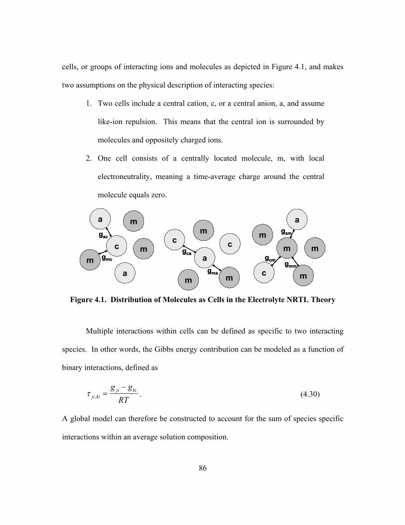
86
cells, or groups of interacting ions and molecules as depicted in Figure 4.1, and makes
two assumptions on the physical description of interacting species:
1. Two cells include a central cation, c, or a central anion, a, and assume
like-ion repulsion. This means that the central ion is surrounded by
molecules and oppositely charged ions.
2. One cell consists of a centrally located molecule, m, with local
electroneutrality, meaning a time-average charge around the central
molecule equals zero.
m m
mm
m
m
mcc c
c
a
a
a
a
m
m
m gcagcm gmm
gac
gmc
gma
gam
m m
mm
m
m
mcc c
c
a
a
a
a
m
m
m gcagcm gmm
gac
gmc
gma
gam
Figure 4.1. Distribution of Molecules as Cells in the Electrolyte NRTL Theory
Multiple interactions within cells can be defined as specific to two interacting
species. In other words, the Gibbs energy contribution can be modeled as a function of
binary interactions, defined as
,ji ki
ji ki
g gRT
τ−
= . (4.30)
A global model can therefore be constructed to account for the sum of species specific
interactions within an average solution composition.

87
The excess Gibbs energy is predicted from the NRTL theory as
' , ' , '
' " , '"
' , ' ,
' " , '"
j jm jm a jc a c jc a cexj jNRTL
m cm c ak km a k kc a c
k a k
c ja c a ja caj
aa c c k ka c a
c k
X G X Gg X XRT X G X X G
X GX
X X G
τ τ
τ
= + +
∑ ∑∑ ∑ ∑∑ ∑ ∑
∑∑ ∑ ∑ ∑
, (4.31)
where
∑∑
=
''
,
aa
amcaa
cm X
GXG ,
∑∑
=
''
,
cc
cmcac
cm X
GXG , (4.32)
( )cajccajccajcG ',',', exp τα−= , ( )acjaacjaacjaG ',',', exp τα−= , (4.33)
and
( )imimimG τα−= exp , ( )mcamcamcaG ,,, exp τα−= , (4.34)
∑∑
=
''
,
aa
amcaa
cm X
X αα ,
∑∑
=
''
,
cc
cmcac
am X
X αα . (4.35)
Also, cammcaamcama ,,, ττττ +−= , cammcacmacmc ,,, ττττ +−= , jjj CxX = (Cj = Zj for ions
and 1 for molecules), α is the nonrandomness parameter, and τ is the binary interaction
parameter.
The reference state of the NRTL contribution can be converted to the
unsymmetric convention with the correction of infinite dilution activity coefficients.
*
ln ln lnex exNRTL NRTL
m m c c a am w c a
g g x x xRT RT
γ γ γ∞ ∞ ∞
≠
= − + + ∑ ∑ ∑ (4.36)
where
88
ln m wm mw mwGγ τ τ∞ = + (4.37)
' , ''
""
lna wc a c
ac c cw cw
aa
xZ G
x
τγ τ∞
= +
∑∑
(4.38)
' , ''
""
lnc wa c a
ca a aw aw
cc
xZ G
x
τγ τ∞
= +
∑∑
(4.39)
The subscript w represents water.
4.1.4. Thermodynamic Model Default Settings
For modeling K+/PZ mixtures in this work, nonrandomness parameters for
molecule-molecule pairs and water-ion pairs were set to 0.2 according to the
recommendation of Renon and Prausnitz (1968). For amine-ion pairs, values were set
to 0.1. Molecule-molecule interaction parameters (τ) are given by
( )KTBA +=τ . (4.40)
The default value of A is 0.0 and the default temperature dependence, B, is 0.0. The
interaction parameters for molecule-ion pair and ion pair-molecule are given by
( ) ( )
−+=
KKTBA
15.35311τ (4.41)
with default values for A of 15.0 and �8.0 respectively. If the molecule is water, the
values are 8.0 and �4.0. The default temperature dependence, B, is 0.0. Ion pair-ion
pair interactions are normally insignificant and not included in this model.
89
4.1.5. Vapor-Liquid Equilibrium
Recall that equilibrium with the vapor phase is represented in terms of fugacity,
a function of concentration and pressure.
Pyf iiv
i φ�� = (4.42)
where
Pyf
i
vi
i
�� =φ (4.43)
More exactly, as an extension of residual properties, φ can be written as
0
�ln 1P
ii
PV dPRT P
φ = − ∫ . (4.44)
An equation of state (EOS) is needed to describe the molar volume, Vi.
The Redlich-Kwong-Soave (RKS) equation of state was chosen for this work
(Soave, 1972). This expression can be written as pressure explicit,
( )( )
,a TRTPV b V V b
ω= −
− +, (4.45)
or as cubic in terms of volume.
( )( ) ( )23 2
, ,0
a T bRT Pb a T bRTV V VP P P
α ω α ω− −− + − = (4.46)
T and P represent the temperature and pressure of the vapor phase and R represents the
gas constant. The attraction between molecules and their size are represented in the
equation by parameters a and b respectively.
90
In Equation (4.46), a is a function of temperature and the acentric factor, ω, and
can be written
( ) ( ), ,a T a Tω α ω= , (4.47)
where
( ) ( )[ ]25.011, rTfT −+= ωωα , (4.48)
and
215613.055171.148508.0 ωωω −+=f . (4.49)
The terms α and fω were determined empirically to fit known vapor pressures. The
parameter b is calculated as in the original Redlich-Kwong equation
0.086640 C
C
RTbP
= , (4.50)
where TC and PC represent the critical temperature and pressure.
Expressions for a and b for gas mixtures were developed by Redlich and Kwong
(1948) and are applied in the model.
( )∑∑=i j
jjiijimix aaxxa 5.0αα (4.51)
∑=i
iimix bxb (4.52)
Application of the mixing rules allows the calculation of vapor phase fugacity
from Equation (4.42). The equilibrium model solves Equation (4.46) using a Newton-
Raphson method where the initial guess for V is obtained from the ideal gas law.
91
4.1.6. Reference States
In this work, the reference state for water and PZ is described by the symmetric
convention. This means the activity coefficient of water (or PZ) is defined so that
1 as 1w wxγ → → . (4.53)
CO2, ions, and H+PZCOO- are described by the nonsymmetric convention, meaning the
activity coefficients are referenced to pure water so that
* 1 as 0i ixγ → → . (4.54)
The two conventions are related by
* 0lim
i
ii ix
i
γ γ γγ
∞
→= = , (4.55)
where iγ ∞ represents the symmetrically normalized activity coefficient of solute i, or the
value of γi as the solution approaches its pure water reference state.
The structure of the model treats PZ as a solvent, resulting in two definitions of
equilibrium constants that contain PZ. Constants are normally reported in literature as
referenced to infinite dilution in water and can be represented as
3 3
2 2
* **
* *
Am AmH O H OAm
H O H OAmH AmH
x xK
x x
γ γ
γ γ+ +
+ +
= ⋅ . (4.56)
The constants utilized in the model are normalized so that
3 3
2 2
*
* *
Am AmH O H OAm
H O H OAmH AmH
x xK
x x
γ γ
γ γ+ +
+ +
= ⋅ . (4.57)
92
The constants are therefore related by
* **Am
Am Am Am AmAm
K K Kγ γγ
∞= = . (4.58)
Equilibrium constants reported in this work must be corrected for the infinite dilution
activity coefficient of the amine prior to comparison with other work. An estimate of
PZγ ∞ is presented in Chapter 5.
Also of note is that PZ is considered a liquid. While the melting point is 106oC,
it was assumed that liquid phase properties more adequately represent PZ behavior in
aqueous solution. The requirement of this assumption is that the vapor pressure of PZ is
represented by liquid PZ. The consequence of this assumption is that equilibrium
constants, enthalpies, and other properties relating to PZ behavior are referenced to the
liquid form of the amine (e.g. heat of dissolution is not considered).
4.1.7. Solution Method (Non-Stoichiometric Method)
A non-stoichiometric solution method was used to solve for the equilibrium
composition of K+/PZ mixtures from total system properties (total PZ and K+, total CO2,
and temperature). By defining the activity coefficients and equilibrium constants
through a rigorous model, such as the ENRTL model, the Gibbs energy of the solution
can be calculated. For a defined system, the algorithm minimizes the Gibbs free energy
within the constraints of material balances. The Gibbs energy is related to the chemical
potential, and thus the activity coefficients, as presented in Section 4.1.2.
For K+/PZ mixtures, there are eleven unknown species to be considered.
Potassium ion, though constant, is considered an unknown to increase model flexibility
93
for future applications. Hydronium ion (H3O+) is neglected because its concentration is
assumed to be very small. Five elements are identified for the material balances: K+,
PZ, C, H, and O. PZ (minus the hydrogens) can be considered an element because the
core of the molecule is constant. The material balances are then
( )
( )
2
22 3 32
2 3
22 2 3 3
,
,
,
,
2
2 2 3 2
2 3 3 2
K K Tot
PZ PZ TotPZH PZCOO H PZCOO PZ COO
CO C TotCO HCO PZCOO H PZCOO PZ COO
H O PZ H TotOH HCO PZH PZCOO H PZCOO
H O COOH CO HCO PZC
n n
n n n n n n
n n n n n n n
n n n n n n n n
n n n n n n
+ +
+ − + − −
− − − + − −
− − + − + −
− − −
=
+ + + + =
+ + + + + =
+ + + + + + =
+ + + + + ( )2
,2 4 O TotOO H PZCOO PZ COOn n n− + − −
+ + =
. (4.59)
Lagrangian multipliers, λ, are used for each element so that the chemical
potential of each species can be expressed as
( )
2
2
3
23
2
2 0
0
2 0
3 0
3 0
0
2 03 0
2 0
2 2 0
2 4 0
CO C O
K K
H O H O
C H OHCO
C OCO
H OOH
PZ PZ H
PZ HPZH
PZ C H OPZCOO
PZ C H OH PZCOO
PZ C OPZ COO
µ λ λ
µ λ
µ λ λ
µ λ λ λ
µ λ λ
µ λ λ
µ λ λµ λ λ
µ λ λ λ λ
µ λ λ λ λ
µ λ λ λ
+ +
−
−
−
+
−
+ −
−
− − =
− = − − = − − − = − − = − − = − − = − − =
− − − − = − − − − = − − − =
. (4.60)
This gives eleven equations, dependent upon chemical potential, to be solved
simultaneously. The chemical potentials are minimized and an equilibrium composition
is determined. A more thorough discussion of the non-stoichiometric method and the
solution algorithm by Smith and Missen (1988) can be found in Austgen (1989).

94
4.2. Kinetic/Rate Model
4.2.1. Introduction
A substantial amount of research on CO2 absorption by amines has been
published in the open literature. With each new solvent or solvent blend, new
challenges of representing solvent behavior arise, leading to a better understanding of
the fundamental processes in gas absorption. A rigorous analysis of the experimental
data is imperative to arrive at a complete picture of the solution behavior.
Bishnoi (2000) programmed a rigorous mass transfer model to quantify and
interpret experimental results on a fundamental level by simulating the absorption of
gas into a reactive liquid. The model corrects for gas film resistance and uses the eddy
diffusivity theory to describe mass transfer with chemical reaction in the liquid
boundary layer. This work extends the model for a K+/PZ mixture.
The problem is calculating the flux of CO2 into or out of the solvent by
considering temperature, total solvent composition, the gas and liquid film mass transfer
coefficients, and the bulk gas partial pressure. The model iteratively solves for the
concentration profiles of all species in solution across the boundary layer. Through
material balances and reaction rates, a flux is predicted, which is directly related to the
diffusion of reactants and products and the kinetics of reacting species. Values of
diffusion coefficients and rate constants are obtained by fitting the model to
experimental data.
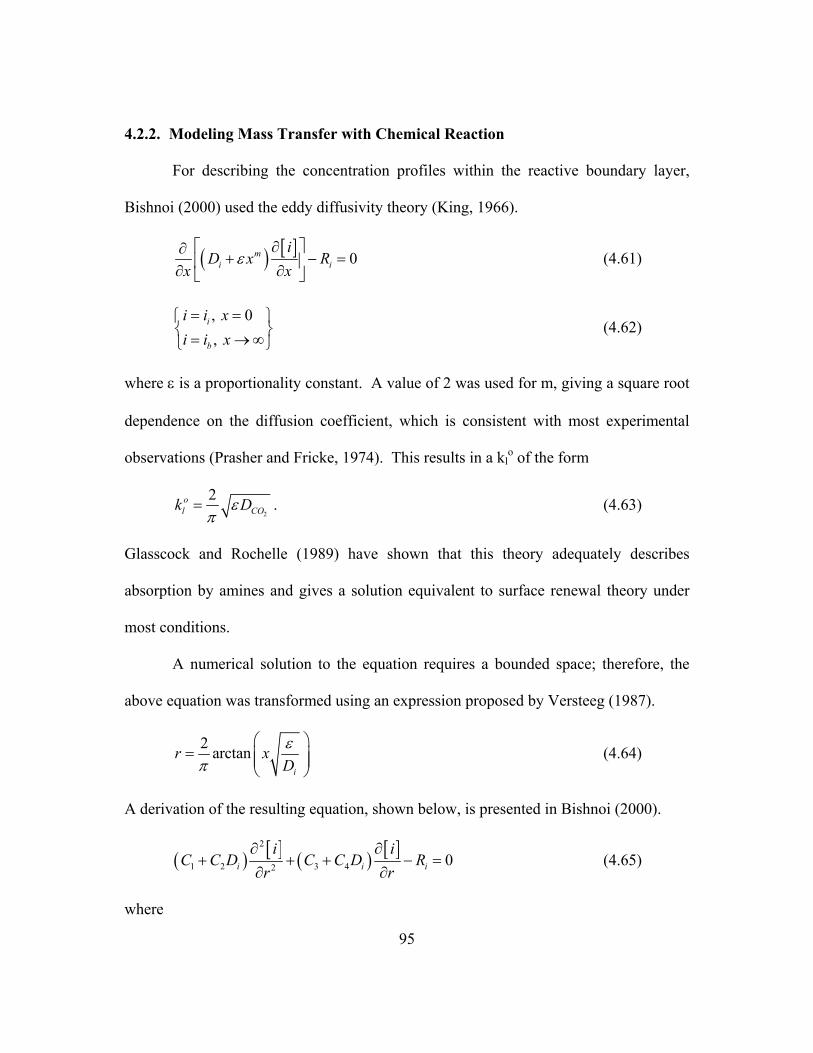
95
4.2.2. Modeling Mass Transfer with Chemical Reaction
For describing the concentration profiles within the reactive boundary layer,
Bishnoi (2000) used the eddy diffusivity theory (King, 1966).
( ) [ ] 0mi i
iD x R
x xε
∂∂+ − = ∂ ∂
(4.61)
, 0,
i
b
i i xi i x
= = = → ∞
(4.62)
where ε is a proportionality constant. A value of 2 was used for m, giving a square root
dependence on the diffusion coefficient, which is consistent with most experimental
observations (Prasher and Fricke, 1974). This results in a klo of the form
2
2ol COk Dε
π= . (4.63)
Glasscock and Rochelle (1989) have shown that this theory adequately describes
absorption by amines and gives a solution equivalent to surface renewal theory under
most conditions.
A numerical solution to the equation requires a bounded space; therefore, the
above equation was transformed using an expression proposed by Versteeg (1987).
2 arctani
r xDε
π
=
(4.64)
A derivation of the resulting equation, shown below, is presented in Bishnoi (2000).
( ) [ ] ( ) [ ]2
1 2 3 42 0i i i
i iC C D C C D R
r r∂ ∂
+ + + − =∂ ∂
(4.65)
where
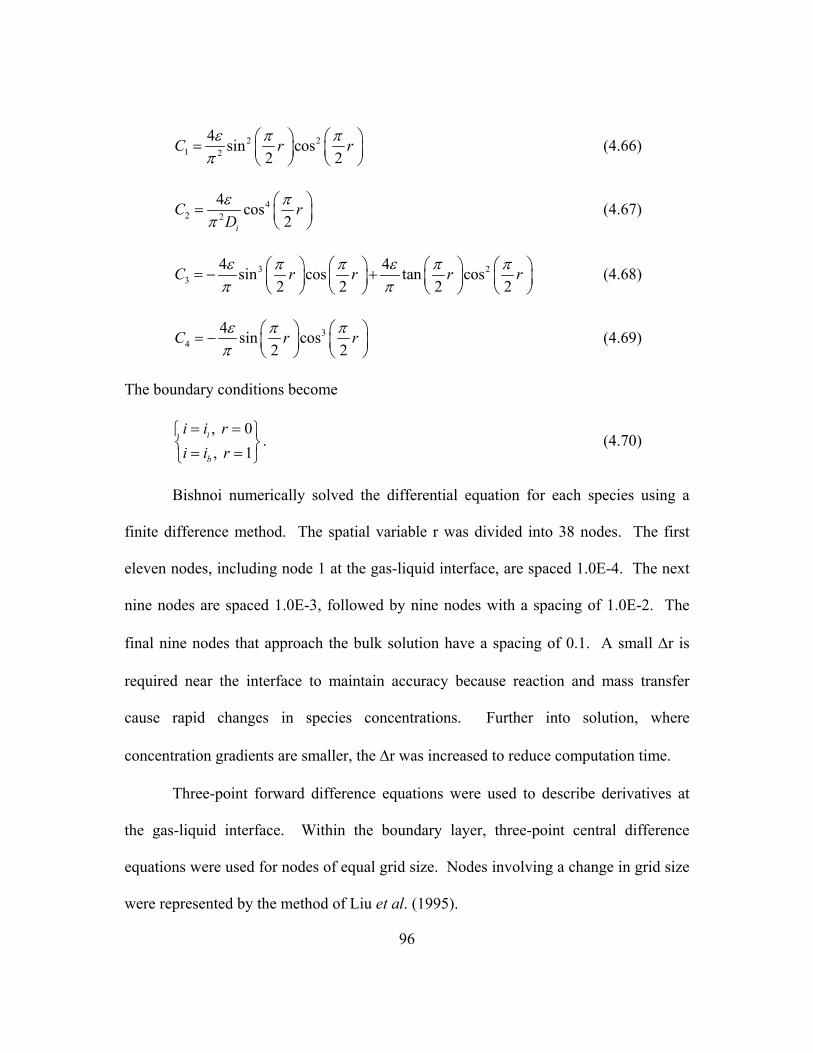
96
2 21 2
4 sin cos2 2
C r rε π ππ
=
(4.66)
42 2
4 cos2i
C rDε π
π =
(4.67)
3 23
4 4sin cos tan cos2 2 2 2
C r r r rε π π ε π ππ π
= − +
(4.68)
34
4 sin cos2 2
C r rε π ππ
= −
(4.69)
The boundary conditions become
, 0, 1
i
b
i i ri i r
= = = =
. (4.70)
Bishnoi numerically solved the differential equation for each species using a
finite difference method. The spatial variable r was divided into 38 nodes. The first
eleven nodes, including node 1 at the gas-liquid interface, are spaced 1.0E-4. The next
nine nodes are spaced 1.0E-3, followed by nine nodes with a spacing of 1.0E-2. The
final nine nodes that approach the bulk solution have a spacing of 0.1. A small ∆r is
required near the interface to maintain accuracy because reaction and mass transfer
cause rapid changes in species concentrations. Further into solution, where
concentration gradients are smaller, the ∆r was increased to reduce computation time.
Three-point forward difference equations were used to describe derivatives at
the gas-liquid interface. Within the boundary layer, three-point central difference
equations were used for nodes of equal grid size. Nodes involving a change in grid size
were represented by the method of Liu et al. (1995).
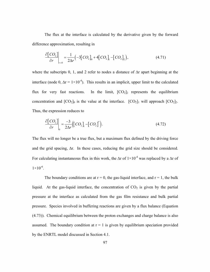
97
The flux at the interface is calculated by the derivative given by the forward
difference approximation, resulting in
[ ] [ ] [ ] [ ]( )22 2 20 1 2
0
1 3 42
r
COCO CO CO
r r=
∂= − + −
∂ ∆, (4.71)
where the subscripts 0, 1, and 2 refer to nodes a distance of ∆r apart beginning at the
interface (node 0, ∆r = 1×10⁻⁴). This results in an implicit, upper limit to the calculated
flux for very fast reactions. In the limit, [CO2]2 represents the equilibrium
concentration and [CO2]0 is the value at the interface. [CO2]1 will approach [CO2]2.
Thus, the expression reduces to
[ ] [ ] [ ]( )*22 2
0
32 i
COCO CO
r r∂ −
= −∂ ∆
. (4.72)
The flux will no longer be a true flux, but a maximum flux defined by the driving force
and the grid spacing, ∆r. In these cases, reducing the grid size should be considered.
For calculating instantaneous flux in this work, the ∆r of 1×10⁻⁴ was replaced by a ∆r of
1×10⁻⁶.
The boundary conditions are at r = 0, the gas-liquid interface, and r = 1, the bulk
liquid. At the gas-liquid interface, the concentration of CO2 is given by the partial
pressure at the interface as calculated from the gas film resistance and bulk partial
pressure. Species involved in buffering reactions are given by a flux balance (Equation
(4.73)). Chemical equilibrium between the proton exchanges and charge balance is also
assumed. The boundary condition at r = 1 is given by equilibrium speciation provided
by the ENRTL model discussed in Section 4.1.
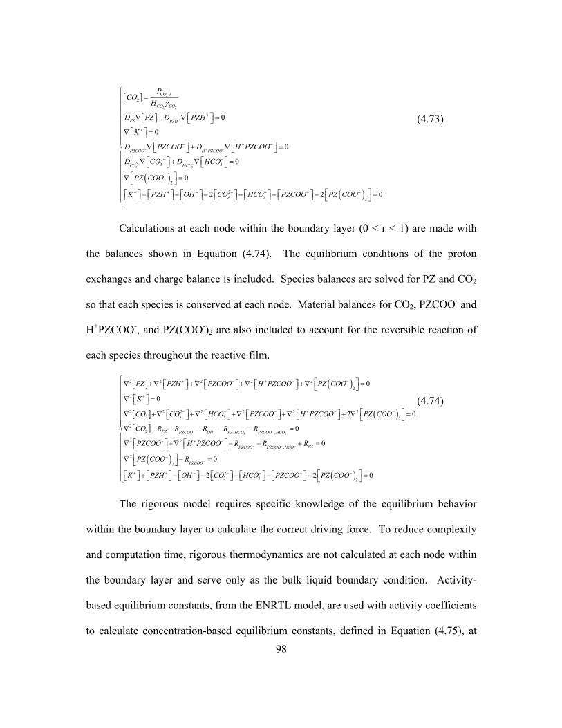
98
[ ]
[ ]
( )
2
2 2
23 3
,2
23 3
2
23 3
0
0
0
0
0
2 2
CO i
CO CO
PZ PZH
PZCOO H PZCOO
CO HCO
PCO
H
D PZ D PZH
K
D PZCOO D H PZCOO
D CO D HCO
PZ COO
K PZH OH CO HCO PZCOO P
γ
+
− + −
− −
+
+
− + −
− −
−
+ + − − − −
=
∇ + ∇ = ∇ =
∇ + ∇ = ∇ + ∇ =
∇ =
+ − − − − − ( )2
0Z COO−
=
(4.73)
Calculations at each node within the boundary layer (0 < r < 1) are made with
the balances shown in Equation (4.74). The equilibrium conditions of the proton
exchanges and charge balance is included. Species balances are solved for PZ and CO2
so that each species is conserved at each node. Material balances for CO2, PZCOO- and
H+PZCOO-, and PZ(COO-)2 are also included to account for the reversible reaction of
each species throughout the reactive film.
[ ] ( )
[ ] ( )[ ]
3 3
2 2 2 2 2
2
2
2 2 2 2 2 2 22 3 3 2
22 , ,
2
0
0
2 0
0PZ PZCOO OH PZ HCO PZCOO HCO
PZ PZH PZCOO H PZCOO PZ COO
K
CO CO HCO PZCOO H PZCOO PZ COO
CO R R R R R
PZCOO
− − − − −
+ − + − −
+
− − − + − −
−
∇ + ∇ + ∇ + ∇ + ∇ = ∇ =
∇ + ∇ + ∇ + ∇ + ∇ + ∇ = ∇ − − − − − =
∇
( )( )
3
2,
2
2
23 3 2
0
0
2 2 0
PZPZCOO PZCOO HCO
PZCOO
H PZCOO R R R
PZ COO R
K PZH OH CO HCO PZCOO PZ COO
− − −
−
+ −
−
+ + − − − − −
+ ∇ − − + =
∇ − = + − − − − − =
(4.74)
The rigorous model requires specific knowledge of the equilibrium behavior
within the boundary layer to calculate the correct driving force. To reduce complexity
and computation time, rigorous thermodynamics are not calculated at each node within
the boundary layer and serve only as the bulk liquid boundary condition. Activity-
based equilibrium constants, from the ENRTL model, are used with activity coefficients
to calculate concentration-based equilibrium constants, defined in Equation (4.75), at
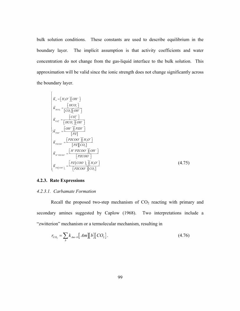
99
bulk solution conditions. These constants are used to describe equilibrium in the
boundary layer. The implicit assumption is that activity coefficients and water
concentration do not change from the gas-liquid interface to the bulk solution. This
approximation will be valid since the ionic strength does not change significantly across
the boundary layer.
[ ]
[ ]
[ ][ ]
( )( )
3
23
2
3
3
2
23
3
3
2
32
w
HCO
CO
PZH
PZCOO
H PZCOO
PZ COO
K H O OH
HCOK
CO OH
COK
HCO OH
OH PZHK
PZ
PZCOO H OK
PZ CO
H PZCOO OHK
PZCOO
PZ COO H OK
PZC
−
−
+
−
+ −
−
+ −
−
−
−
− −
− +
− +
+ − −
−
− +
= =
=
=
=
=
=[ ]2OO CO−
(4.75)
4.2.3. Rate Expressions
4.2.3.1. Carbamate Formation
Recall the proposed two-step mechanism of CO2 reacting with primary and
secondary amines suggested by Caplow (1968). Two interpretations include a
�zwitterion� mechanism or a termolecular mechanism, resulting in
[ ][ ][ ]2 2CO Am b
br k Am b CO−= ∑ . (4.76)
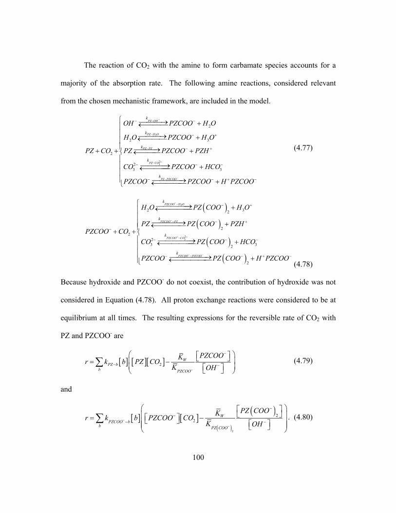
100
The reaction of CO2 with the amine to form carbamate species accounts for a
majority of the absorption rate. The following amine reactions, considered relevant
from the chosen mechanistic framework, are included in the model.
2
23
2
2 3
2
23 3
PZ OH
PZ H O
PZ PZ
PZ CO
PZ PZCOO
k
k
k
k
k
OH PZCOO H O
H O PZCOO H O
PZ CO PZ PZCOO PZH
CO PZCOO HCO
PZCOO PZCOO H PZCOO
−−
−
−
−−
−−
− −
− +
− +
− − −
− − + −
→ +← → +← →+ + + ←
→ +← → +←
(4.77)
( )( )
( )( )
2
23
2 32
22
23 32
2
PZCOO H O
PZCOO PZ
PZCOO CO
PZCOO PZCOO
k
k
k
k
H O PZ COO H O
PZ PZ COO PZHPZCOO CO
CO PZ COO HCO
PZCOO PZ COO H PZCOO
−−
−−
− −−
− −−
− +
− +
−
− − −
− − + −
→ +←
→ + ←+ + → +← → +← (4.78)
Because hydroxide and PZCOO- do not coexist, the contribution of hydroxide was not
considered in Equation (4.78). All proton exchange reactions were considered to be at
equilibrium at all times. The resulting expressions for the reversible rate of CO2 with
PZ and PZCOO- are
[ ] [ ][ ]2W
PZ bb PZCOO
PZCOOKr k b PZ COK OH−
−
− −
= −
∑ (4.79)
and
[ ] [ ]( )
( )
2
22
WPZCOO b
b PZ COO
PZ COOKr k b PZCOO COK OH
−
−
−
−−−
= −
∑ . (4.80)

101
The temperature dependence of these rate constants is given by
( )1 1exp
298.15o aHk k
R T K∞
−∆= −
, (4.81)
where k∞ represents the rate constant in the absence of significant ionic strength, ko is
the specific rate constant, and ∆Ha is the activation energy for the specific reaction.
The values of all regressed model parameters from this work are presented in
Chapter 6. Parameters include the above rate constants, an activation energy (assumed
constant for all amine-base reactions), and a correction for ion diffusivities.
4.2.3.2. Bicarbonate Formation
Based on work with tertiary amines and experience with base-catalyzed
reactions, amines and hydroxide are expected to catalyze the formation of bicarbonate
ion (Littel et al., 1990b; Bishnoi, 2000). Three parallel reactions are included in the
model to account for this effect.
2 3OH
kCO OH HCO
−− −→+ ← (4.82)
2 2 3PZkPZ CO H O PZH HCO+ −→+ + +← (4.83)
2 2 3PZCOO
kPZCOO CO H O H PZCOO HCO
−− + − −→+ + +← (4.84)
The formation of bicarbonate in this manner is typically much slower than the reaction
of CO2 with amines and has little effect on the absorption rate under most conditions,
but must be included to properly model equilibrium in the boundary layer. A
generalized, second-order rate expression for these reactions can be written as
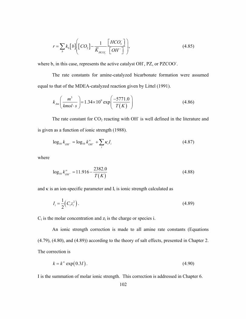
102
[ ] [ ]3
32
1b
b HCO
HCOr k b CO
K OH−
−
−
= −
∑ , (4.85)
where b, in this case, represents the active catalyst OH-, PZ, or PZCOO-.
The rate constants for amine-catalyzed bicarbonate formation were assumed
equal to that of the MDEA-catalyzed reaction given by Littel (1991).
( )3
9 5771.01.34 10 expAmmk
kmol s T K −
= × ⋅ (4.86)
The rate constant for CO2 reacting with OH- is well defined in the literature and
is given as a function of ionic strength (1988).
10 10log log i iOH OHi
k k Iκ− −∞= + ∑ (4.87)
where
( )102382.0log 11.916
OHk
T K−∞ = − (4.88)
and κ is an ion-specific parameter and Ii is ionic strength calculated as
( )212i i iI C z= . (4.89)
Ci is the molar concentration and zi is the charge or species i.
An ionic strength correction is made to all amine rate constants (Equations
(4.79), (4.80), and (4.89)) according to the theory of salt effects, presented in Chapter 2.
The correction is
( )exp 0.3k k I∞= . (4.90)
I is the summation of molar ionic strength. This correction is addressed in Chapter 6.
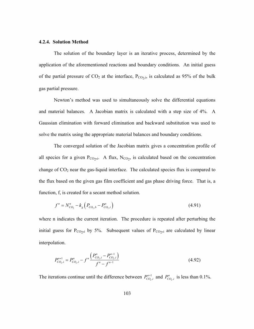
103
4.2.4. Solution Method
The solution of the boundary layer is an iterative process, determined by the
application of the aforementioned reactions and boundary conditions. An initial guess
of the partial pressure of CO2 at the interface, PCO2,i, is calculated as 95% of the bulk
gas partial pressure.
Newton�s method was used to simultaneously solve the differential equations
and material balances. A Jacobian matrix is calculated with a step size of 4%. A
Gaussian elimination with forward elimination and backward substitution was used to
solve the matrix using the appropriate material balances and boundary conditions.
The converged solution of the Jacobian matrix gives a concentration profile of
all species for a given PCO2,i. A flux, NCO2, is calculated based on the concentration
change of CO2 near the gas-liquid interface. The calculated species flux is compared to
the flux based on the given gas film coefficient and gas phase driving force. That is, a
function, f, is created for a secant method solution.
( )2 2 2, ,n n n
CO g CO b CO if N k P P= − − (4.91)
where n indicates the current iteration. The procedure is repeated after perturbing the
initial guess for PCO2,i by 5%. Subsequent values of PCO2,i are calculated by linear
interpolation.
( )2 2
2 2
1, ,1
, , 1
n nCO i CO in n n
CO i CO i n n
P PP P f
f f
−+
−
−= −
− (4.92)
The iterations continue until the difference between 2
1,
nCO iP + and
2 ,n
CO iP is less than 0.1%.
104
4.3. Non-Linear Regression Model
4.3.1. Description of GREG
The regression of parameters in the thermodynamic and rate models was
performed using the Generalized REGression package, GREG, developed by
Caracotsios (1986). GREG is a multiple parameter, non-linear regression tool that
minimizes the difference between a model calculated value, Fi, that is a function of
given parameter values, xj, and a user-provided observed value, OBSi.
( )2
1
n
i j ii
Obj F x OBS=
= − ∑ (4.93)
Some data, such as the activity of water and mole fractions (speciation data),
were regressed as is. For equilibrium partial pressure data, where the values (Fi(xj))
varied over several decades, a logarithmic transformation of the data (i.e. ln(PCO2*)) was
used to give even weight to all data points. In each case where multiple data sets were
simultaneously regressed, the data types were weighted so that each gave a comparable
contribution to the sum-of-squares error.
The generic character of the model allows its coupling with any user-defined
model. GREG is highly versatile, capable of being applied to the regression of any
model parameter. Parameters regressed in this work include equilibrium constants,
binary interaction parameters, and rate constants.
4.3.2. Interface with the Thermodynamic and Rate Models
GREG is completely external to all other programs. The model, or main
program, is essentially the inner part of a loop that runs once for every observed

105
parameter supplied. The results are stored in an array and returned to GREG for
statistical calculations.
A simple flowsheet is shown in Figure 4.2, showing how GREG interacts with
other programs for i = 1 to n, where n is the number of observed parameters. The
regression driver provides GREG with information important to the regression,
including the initial parameter values (xj), the upper and lower bounds, the maximum
change, and the tolerance for termination of the regression. The observed, or
experimental data, is provided to the regression driver through an input file and
subsequently transferred to GREG. GREG then supplies the necessary parameter
values and executes the main program. The main program reads input from data files
and returns a calculated result, Fi, to GREG. GREG changes the values of xj until the
objective function is minimized and a final solution is obtained.
RegressionDriver GREG
MainProgram
Input &Data
OBSiModelInput
RegessionParameters
Fi
xj
Figure 4.2. Transfer of Data during a Regression with GREG
106
4.3.3. Results and Statistics from GREG
In addition to the parameter values and sum of squares, a confidence interval
and correlation parameters were calculated. An understanding of these values improves
the significance and clarity of the regressed parameters for representing a given data set.
A confidence interval was calculated for each given mean parameter value, x .
The confidence interval expresses the certainty of which the true value of a parameter is
known. In this work, the confidence interval is reported as a standard deviation, σ. The
standard deviation is calculated as
( )2
1
11
n
x jj
x xn
σ=
= −− ∑ . (4.94)
GREG also calculates a correlation matrix, which identifies potential
interference from the dependence of regressed parameters on each other. The
correlation between two variables, x and y, is given by the correlation coefficient,
ρ(x,y).
( ) ( ),,
x y
Cov x yx yρ
σ σ= (4.95)
where Cov(x,y), the covariance, is calculated as
( ) ( )( )1
1,1
n
j jj
Cov x y x x y yn =
= − −− ∑ . (4.96)
The covariance quantifies the linear relationship between variables x and y. An
important constraint is that the absolute value of covariance is always less than the
product of standard deviations.
107
( ), x yCov x y σ σ≤ (4.97)
Also, the covariance is symmetric, so that
( ) ( ), ,Cov x y Cov y x= . (4.98)
Thus, the correlation coefficient is bounded between -1 and 1. Values of ρ(x,y) of -1
and 1 indicate perfectly correlated parameters, meaning x and y are linearly dependent.
Small values (i.e. ( ), 0x yρ → ) indicate completely independent values of x and y.
108
Equation Chapter 5 Section 1
Chapter 5: Thermodynamics of Potassium Carbonate,
Piperazine, and Carbon Dioxide Mixtures
Absorption processes incorporating various aqueous amine solvents have long
been known as effective for the treatment of waste gas streams, particularly for
removing acidic components (CO2, H2S). For any new or existing solvent, an
understanding of the thermodynamics and the ability to model equilibrium behavior is
important for process development, design, and optimization. This chapter examines
thermodynamic properties attained by blending PZ with K2CO3 in a concentrated
aqueous mixture.
Measurements of CO2 solubility in a wetted-wall column in 0.6 to 3.6 m PZ and
2.5 to 6.2 m K+ at 40 to 110oC are presented. Piperazine speciation was also determined
using 1H NMR for 0.6 to 3.6 m PZ and 3.6 to 6.2 m K+ at 25 to 70oC and the results are
reported here. Other thermochemical properties, the physical solubility of CO2 and the
109
solid solubility of the potassium salt and the piperazine solid, were also explored and
reported.
As discussed in Chapter 4, a rigorous thermodynamic model of aqueous
potassium carbonate/piperazine was developed to describe the vapor- and liquid-phase
equilibrium of the solvent with CO2. The model was sequentially fitted to a variety of
data, beginning with simple binary systems and extending to complex, multi-component
electrolyte mixtures. Representation of the VLE and speciation is achieved and
demonstrated over the range of solvents investigated. Predictions of
thermodynamically significant properties, such as solvent capacity, heat of absorption,
and stoichiometric behavior are presented.
5.1. Model Description
Eight equilibrium reactions, shown below, are included in the model for K+/PZ.
The equilibrium constants for reactions (5.1) through (5.4) are shown in Table 5.1.
Constants for reactions (5.5) through (5.7) were regressed from experimental data and
are presented in Section 5.4.3.
( )2 2 3 32CO aq H O HCO H O− +→+ ⋅ +← (5.1)
23 2 3 3HCO H O CO H O− − +→+ +← (5.2)
2 32 H O H O OH+ −→⋅ +← (5.3)
( )2 3PZH H O PZ l H O+ +→+ +← (5.4)
( ) ( )2 2 3PZ l CO aq H O PZCOO H O− +→+ + +← (5.5)
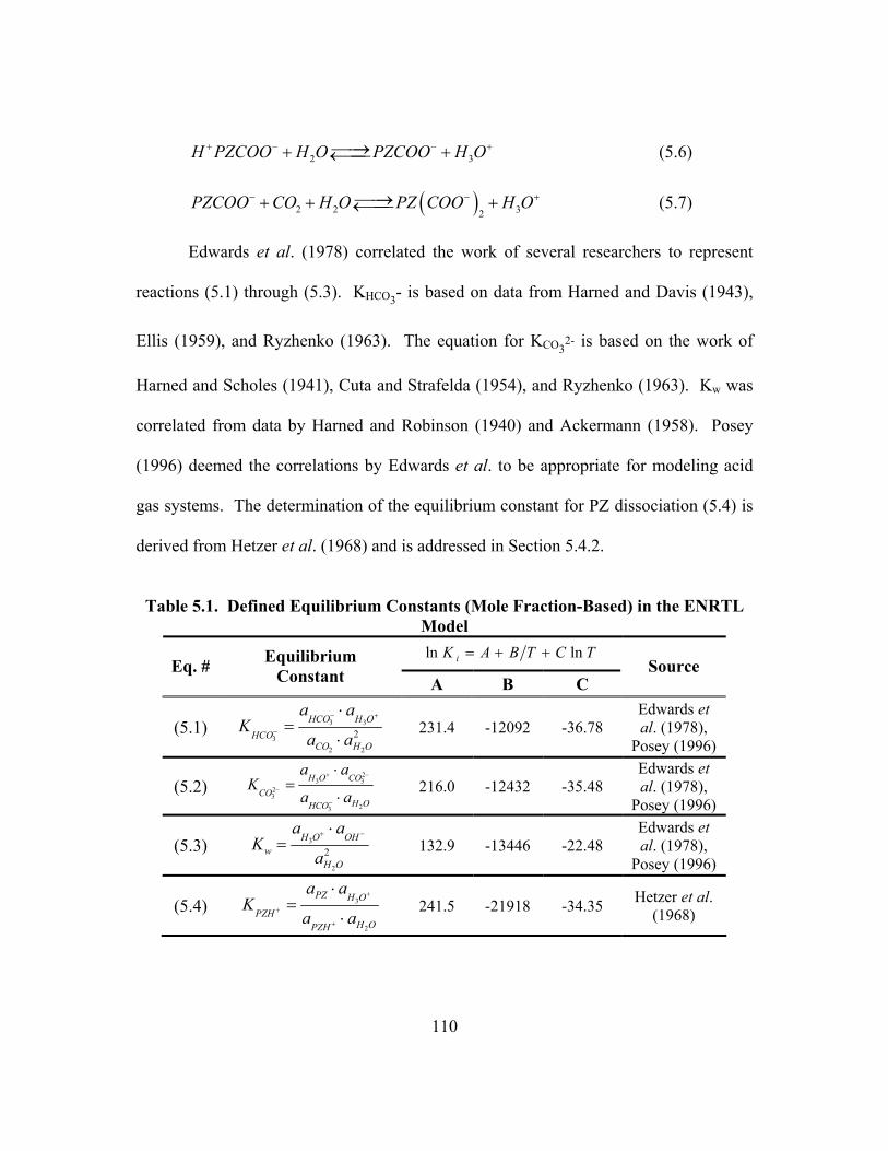
110
2 3H PZCOO H O PZCOO H O+ − − +→+ +← (5.6)
( )2 2 32PZCOO CO H O PZ COO H O− − +→+ + +← (5.7)
Edwards et al. (1978) correlated the work of several researchers to represent
reactions (5.1) through (5.3). KHCO3- is based on data from Harned and Davis (1943),
Ellis (1959), and Ryzhenko (1963). The equation for KCO32- is based on the work of
Harned and Scholes (1941), Cuta and Strafelda (1954), and Ryzhenko (1963). Kw was
correlated from data by Harned and Robinson (1940) and Ackermann (1958). Posey
(1996) deemed the correlations by Edwards et al. to be appropriate for modeling acid
gas systems. The determination of the equilibrium constant for PZ dissociation (5.4) is
derived from Hetzer et al. (1968) and is addressed in Section 5.4.2.
Table 5.1. Defined Equilibrium Constants (Mole Fraction-Based) in the ENRTL
Model TCTBAK i lnln ++=
Eq. # Equilibrium Constant A B C
Source
(5.1) 3 3
32 2
2HCO H O
HCOCO H O
a aK
a a− +
−
⋅=
⋅ 231.4 -12092 -36.78
Edwards et al. (1978),
Posey (1996)
(5.2) 2
3 323
23
H O COCO
H OHCO
a aK
a a+ −
−
−
⋅=
⋅ 216.0 -12432 -35.48
Edwards et al. (1978),
Posey (1996)
(5.3) 3
2
2H O OH
wH O
a aK
a+ −⋅
= 132.9 -13446 -22.48 Edwards et al. (1978),
Posey (1996)
(5.4) 3
2
PZ H OPZH
H OPZH
a aK
a a+
+
+
⋅=
⋅ 241.5 -21918 -34.35 Hetzer et al.
(1968)

111
The ENRTL model was fit to experimental data by regressing equilibrium
constants and binary interaction parameters from multiple, independent data sets using
GREG as presented in Chapter 4. A sequential regression, beginning with simple
mixtures and progressing to more complex solutions, was used to maintain
thermodynamic consistency. Table 5.2 summarizes the sequence and data types used in
the regressions. Table 5.3 reports the regressed parameters and values from each step.
Table 5.2. Summary of Data and Sources for the Regression of Parameters in the
ENRTL Model
# Name Data Type Conc. (m) T (oC) Source(s) Data
Pts.a K2CO3: 0.0 � 1.25 KHCO3: 0.0 � 1.25 25
Joosten and Danckwerts
(1972) 8
1 CO2 N2O
Solubility K2CO3: 0.0 � 2.4 KHCO3: 0.0 � 3.6
PZ: 0.0 � 1.8 25 This Work 18
K2CO3: 0.4 � 7.5 25 � 90 Puchkov and Kurochkina
(1970) 42 2 K2CO3/H2O PH2O*
K2CO3: 0.15 � 7.2 25 - 140 Aseyev (1999) 614
3 KHCO3/H2O PCO2* K2CO3: 1.8 � 4.8 Conv.: 0 � 87%b 70 - 140 Tosh et al.
(1959) 120
4 PZ/H2O UNIFAC PZ: 0 � 2.4 25 - 80 Gmehling (1982) 21
NMR PZ: 0.1 � 1.48 α: 0.15 � 1.0c 20 - 60 Ermatchkov et
al. (2003) 218
PTOT PZ: 2 � 4 α: 0.5 � 1.0c 40 - 120 Kamps et al.
(2003) 29 5 PZ/CO2/H2O
PCO2* PZ: 0.64 α: 0.3 � 1.0c 40 - 70 Bishnoi (2000) 17
NMR K2CO3: 3.6 � 6.2
PZ: 0.6 � 3.6 α: 0.35 � 0.7c
27 � 70 This Work 112
6 PZ/K+/CO2/H2O
PCO2* K2CO3: 2.5 � 6.2
PZ: 0.6 � 3.6 α: 0.35 � 0.76c
40 - 110 This Work 58
a. Total number of data points used in the regression. b. Conversion to KHCO3 as reported by Tosh et al. (1959). c. α is loading as defined by mol CO2/(mol K+ + mol PZ).
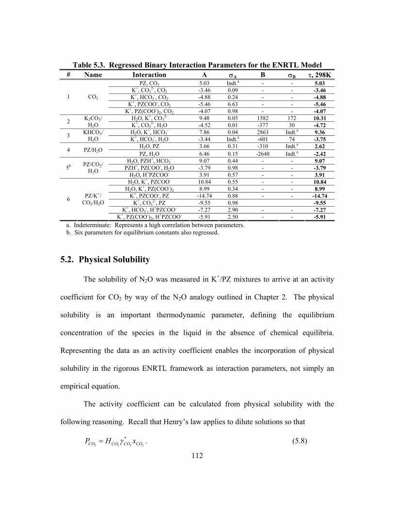
112
Table 5.3. Regressed Binary Interaction Parameters for the ENRTL Model # Name Interaction A σA B σB τ, 298K
PZ, CO2 5.03 Indt.a - - 5.03 K+, CO3
2-, CO2 -3.46 0.09 - - -3.46 K+, HCO3
-, CO2 -4.88 0.24 - - -4.88 K+, PZCOO-, CO2 -5.46 6.63 - - -5.46
1 CO2
K+, PZ(COO-)2, CO2 -4.07 0.98 - - -4.07 H2O, K+, CO3
2- 9.48 0.05 1582 172 10.31 2 K2CO3/ H2O K+, CO3
2-, H2O -4.52 0.01 -377 30 -4.72 H2O, K+, HCO3
- 7.86 0.04 2863 Indt.a 9.36 3 KHCO3/ H2O K+, HCO3
-, H2O -3.44 Indt.a -601 74 -3.75 H2O, PZ 3.66 0.31 -310 Indt.a 2.62 4 PZ/H2O PZ, H2O 6.46 0.15 -2648 Indt.a -2.42
H2O, PZH+, HCO3- 9.07 0.44 - - 9.07
PZH+, PZCOO-, H2O -3.79 0.98 - - -3.79 5b PZ/CO2/ H2O
H2O, H+PZCOO- 3.91 0.57 - - 3.91 H2O, K+, PZCOO- 10.84 0.55 - - 10.84
H2O, K+, PZ(COO-)2 8.99 0.34 - - 8.99 K+, PZCOO-, PZ -14.74 0.88 - - -14.74
K+, CO32-, PZ -9.55 0.98 -9.55
K+, HCO3-, H+PZCOO- -7.27 2.90 - - -7.27
6 PZ/K+/ CO2/H2O
K+, PZ(COO-)2, H+PZCOO- -5.91 2.50 - - -5.91 a. Indeterminate: Represents a high correlation between parameters. b. Six parameters for equilibrium constants also regressed.
5.2. Physical Solubility
The solubility of N2O was measured in K+/PZ mixtures to arrive at an activity
coefficient for CO2 by way of the N2O analogy outlined in Chapter 2. The physical
solubility is an important thermodynamic parameter, defining the equilibrium
concentration of the species in the liquid in the absence of chemical equilibria.
Representing the data as an activity coefficient enables the incorporation of physical
solubility in the rigorous ENRTL framework as interaction parameters, not simply an
empirical equation.
The activity coefficient can be calculated from physical solubility with the
following reasoning. Recall that Henry�s law applies to dilute solutions so that
2 2 2 2
*CO CO CO COP H xγ= . (5.8)

113
In this work, infinite dilution in water is the chosen reference state, so 2
*COγ → 1 and the
expression for Henry�s constant in pure water can be written
2
2
2
COwCO
CO
PH
x= . (5.9)
The activity coefficient in the mixed solvent can then be calculated from the ratio of an
apparent Henry�s constant in the mixed solvent and the Henry�s constant in water.
2
2
2
* COCO w
CO
HH
γ = (5.10)
Thus, the solubility of CO2 in this work is interpreted as the Henry�s constant in water
corrected by the activity coefficient of CO2 in the mixed solvent.
The physical solubility of N2O was measured in aqueous PZ and interpreted as
CO2 solubility. The results of these experiments are shown in Table 5.4 and Figure 5.1.
The addition of PZ to water has little effect on the activity coefficient of CO2 at 25 or
40oC. Even in concentrated solutions (~ 1.5 M), γCO2 increases by less than 10%, which
is consistent with previous work on amines (Littel et al., 1992c; Browning and Weiland,
1994; Sada et al., 1978; Versteeg and van Swaiij, 1988). Only a small increase in
activity coefficient could be identified at these low amine concentrations.
The physical solubility of CO2 was also measured in aqueous K2CO3 and
K2CO3/KHCO3 mixtures (30 and 70% of the total molar salt concentration respectively)
at 25oC for comparison with previous work. Results of these experiments are reported
in Table 5.5. Figure 5.2 compares these results to those of Joosten and Danckwerts
(1972), who report the solubility of N2O in equimolar mixtures of K2CO3 and KHCO3,
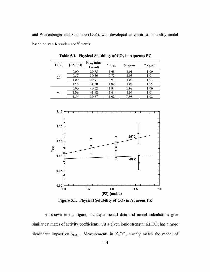
114
and Weisenberger and Schumpe (1996), who developed an empirical solubility model
based on van Krevelen coefficients.
Table 5.4. Physical Solubility of CO2 in Aqueous PZ
T (oC) [PZ] (M) HCO2 (atm-
L/mol) σHCO2
γCO2,meas γCO2,pred
0.00 29.65 1.68 1.01 1.00 0.57 30.36 0.72 1.03 1.01 1.09 29.91 0.91 1.02 1.03
25
1.56 31.60 1.02 1.08 1.05 0.00 40.02 1.94 0.98 1.00 1.09 41.98 1.44 1.03 1.01 40 1.56 39.87 1.02 0.98 1.02
[PZ] (mol/L)0.0 0.5 1.0 1.5 2.0
γ CO
2
0.90
0.95
1.00
1.05
1.10
1.15
40oC
25oC
Figure 5.1. Physical Solubility of CO2 in Aqueous PZ
As shown in the figure, the experimental data and model calculations give
similar estimates of activity coefficients. At a given ionic strength, KHCO3 has a more
significant impact on γCO2. Measurements in K2CO3 closely match the model of

115
Weisenberger and Schumpe (1996). At a constant ionic strength, the activity coefficient
increases as K2CO3 is replaced with KHCO3. Though the solubility in 100% KHCO3
can not be measured experimentally, the model estimation is shown to be consistent
with measured data and gives a higher γCO2.
Table 5.5. Physical Solubility of CO2 in Aqueous K2CO3/KHCO3
[K2CO3] (M)
[KHCO3] (M) I (M)
HCO2 (atm-
L/mol) σHCO2
γCO2,meas γCO2,pred
1.17 0.00 3.51 65.89 3.97 2.24 2.32 1.71 0.00 5.14 96.56 2.54 3.29 3.20 2.23 0.00 6.68 125.77 1.66 4.28 4.20 2.71 0.00 8.12 152.44 20.47 5.19 5.29 0.54 1.27 2.89 71.99 2.32 2.45 2.12 0.76 1.76 4.03 79.54 5.38 2.71 2.70 0.79 1.85 4.22 91.82 14.21 3.13 2.87
I (M)0 2 4 6 8 10
γ CO
2
1
10Schumpe
100% K2CO3
Schumpe100% KHCO3
This Work100% K2CO3
Joosten and Danckwerts50% K2CO3/50% KHCO3
This Work30% K2CO3/70% KHCO3
Figure 5.2. Physical Solubility of CO2 in K2CO3/KHCO3 at 25oC
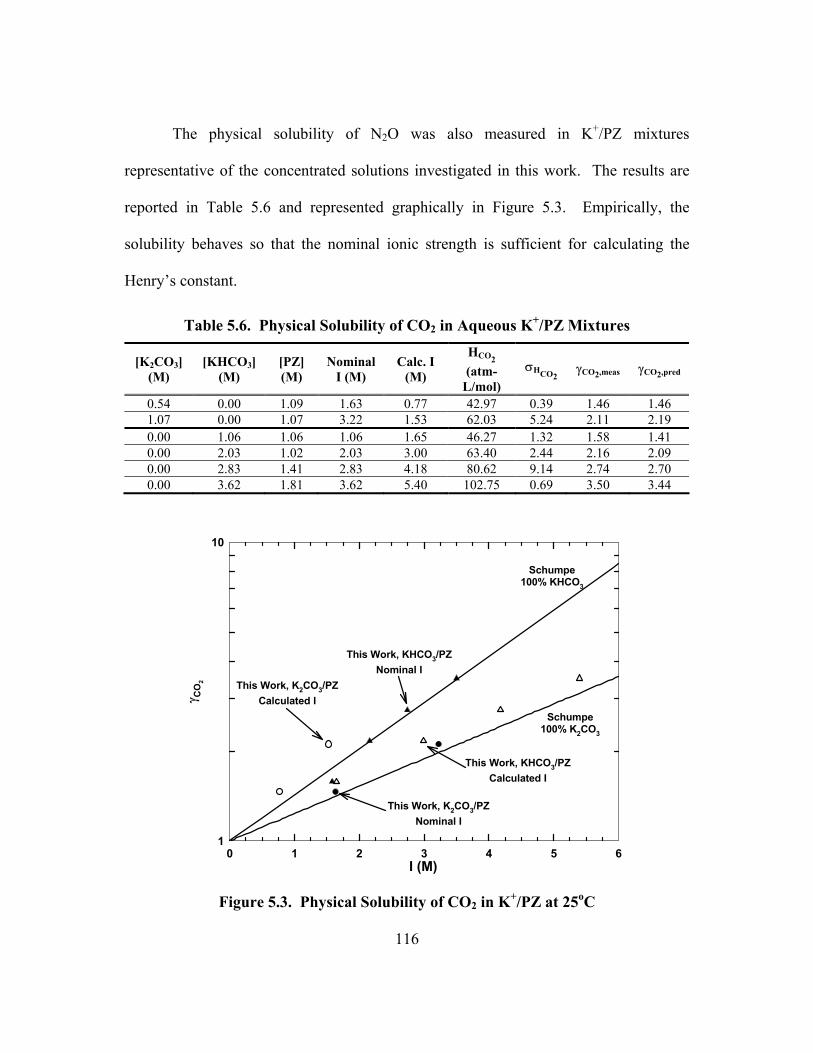
116
The physical solubility of N2O was also measured in K+/PZ mixtures
representative of the concentrated solutions investigated in this work. The results are
reported in Table 5.6 and represented graphically in Figure 5.3. Empirically, the
solubility behaves so that the nominal ionic strength is sufficient for calculating the
Henry�s constant.
Table 5.6. Physical Solubility of CO2 in Aqueous K+/PZ Mixtures
[K2CO3] (M)
[KHCO3] (M)
[PZ] (M)
Nominal I (M)
Calc. I (M)
HCO2
(atm-L/mol)
σHCO2 γCO2,meas γCO2,pred
0.54 0.00 1.09 1.63 0.77 42.97 0.39 1.46 1.46 1.07 0.00 1.07 3.22 1.53 62.03 5.24 2.11 2.19 0.00 1.06 1.06 1.06 1.65 46.27 1.32 1.58 1.41 0.00 2.03 1.02 2.03 3.00 63.40 2.44 2.16 2.09 0.00 2.83 1.41 2.83 4.18 80.62 9.14 2.74 2.70 0.00 3.62 1.81 3.62 5.40 102.75 0.69 3.50 3.44
I (M)0 1 2 3 4 5 6
γ CO
2
1
10
Schumpe100% K2CO3
Schumpe100% KHCO3
This Work, K2CO3/PZCalculated I
This Work, KHCO3/PZNominal I
This Work, K2CO3/PZNominal I
This Work, KHCO3/PZCalculated I
Figure 5.3. Physical Solubility of CO2 in K+/PZ at 25oC
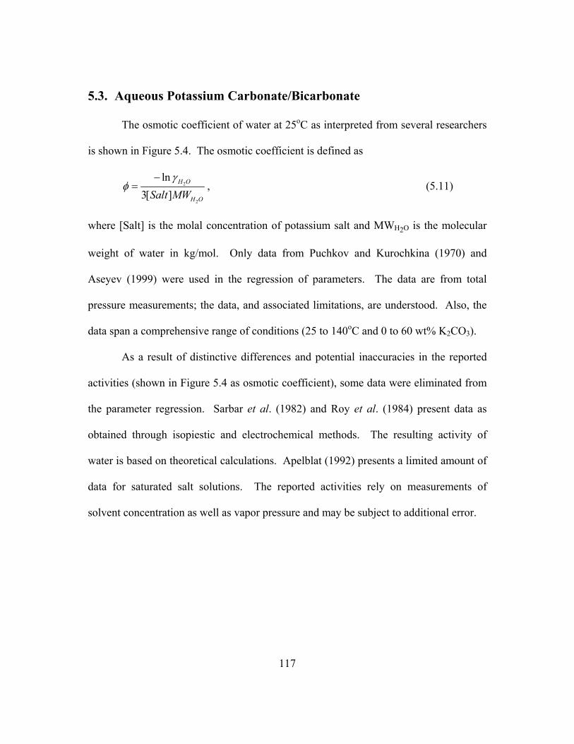
117
5.3. Aqueous Potassium Carbonate/Bicarbonate
The osmotic coefficient of water at 25oC as interpreted from several researchers
is shown in Figure 5.4. The osmotic coefficient is defined as
2
2
ln3[ ]
H O
H OSalt MWγ
φ−
= , (5.11)
where [Salt] is the molal concentration of potassium salt and MWH2O is the molecular
weight of water in kg/mol. Only data from Puchkov and Kurochkina (1970) and
Aseyev (1999) were used in the regression of parameters. The data are from total
pressure measurements; the data, and associated limitations, are understood. Also, the
data span a comprehensive range of conditions (25 to 140oC and 0 to 60 wt% K2CO3).
As a result of distinctive differences and potential inaccuracies in the reported
activities (shown in Figure 5.4 as osmotic coefficient), some data were eliminated from
the parameter regression. Sarbar et al. (1982) and Roy et al. (1984) present data as
obtained through isopiestic and electrochemical methods. The resulting activity of
water is based on theoretical calculations. Apelblat (1992) presents a limited amount of
data for saturated salt solutions. The reported activities rely on measurements of
solvent concentration as well as vapor pressure and may be subject to additional error.
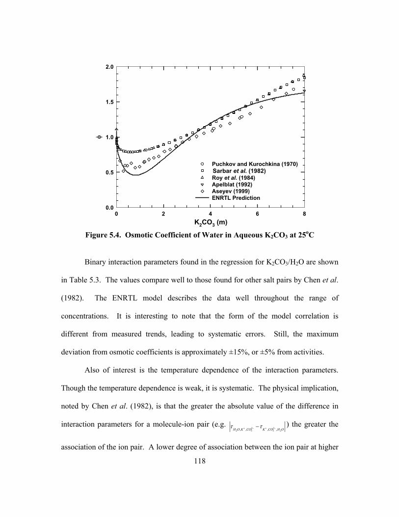
118
K2CO3 (m)0 2 4 6 8
φ
0.0
0.5
1.0
1.5
2.0
Puchkov and Kurochkina (1970) Sarbar et al. (1982)Roy et al. (1984)Apelblat (1992)Aseyev (1999)ENRTL Prediction
Figure 5.4. Osmotic Coefficient of Water in Aqueous K2CO3 at 25oC
Binary interaction parameters found in the regression for K2CO3/H2O are shown
in Table 5.3. The values compare well to those found for other salt pairs by Chen et al.
(1982). The ENRTL model describes the data well throughout the range of
concentrations. It is interesting to note that the form of the model correlation is
different from measured trends, leading to systematic errors. Still, the maximum
deviation from osmotic coefficients is approximately ±15%, or ±5% from activities.
Also of interest is the temperature dependence of the interaction parameters.
Though the temperature dependence is weak, it is systematic. The physical implication,
noted by Chen et al. (1982), is that the greater the absolute value of the difference in
interaction parameters for a molecule-ion pair (e.g. 2 2
2 3 3 2, , , ,H O K CO K CO H Oτ τ+ − + −− ) the greater the
association of the ion pair. A lower degree of association between the ion pair at higher

119
temperatures is expected; thus, molecule-ion pair parameters should have positive
temperature dependence and ion pair-molecule parameters should have negative
temperature dependence. This trend is consistent with the values found in this work.
The equilibrium partial pressure of CO2, PCO2*, reported by Tosh et al. (1959)
was used to regress parameters for KHCO3/H2O mixtures. Data for the mixed solvent
system include 20 to 40 wt% K2CO3 with a range of conversions to KHCO3 at 70 to
140oC. As with the previous regression, the interaction parameters obtained (Table 5.3)
closely resemble behavior demonstrated by other electrolyte systems.
Figure 5.5 and Figure 5.6 show the equilibrium behavior of the mixed solvent at
20 and 40 wt% K2CO3 respectively and 70 to 130oC. The experimental data have a
high degree of scatter, which is also noted by Chen et al. (1979) in an attempt to
represent the data with an extended Pitzer model. Chen et al. also finds the addition of
an ion-ion interaction parameter significantly improves model representation of the
data, suggesting an equivalent parameter in the ENRTL model may improve the fit.
Yet, the ENRTL model adequately represents the data set using only molecule-ion
parameters, deviating by an average of 13.9% over the entire range of conditions.
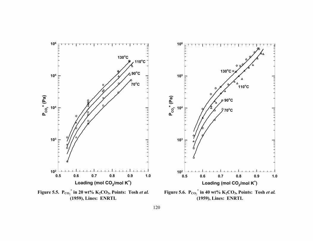
120
Loading (mol CO2/mol K+)0.5 0.6 0.7 0.8 0.9 1.0
P CO
2* (Pa
)
102
103
104
105
106
70oC
90oC
110oC130oC
Figure 5.5. PCO2
* in 20 wt% K2CO3, Points: Tosh et al. (1959), Lines: ENRTL
Loading (mol CO2/mol K+)0.5 0.6 0.7 0.8 0.9 1.0
P CO
2* (Pa
)102
103
104
105
106
70oC
90oC
110oC
130oC
Figure 5.6. PCO2
* in 40 wt% K2CO3, Points: Tosh et al. (1959), Lines: ENRTL
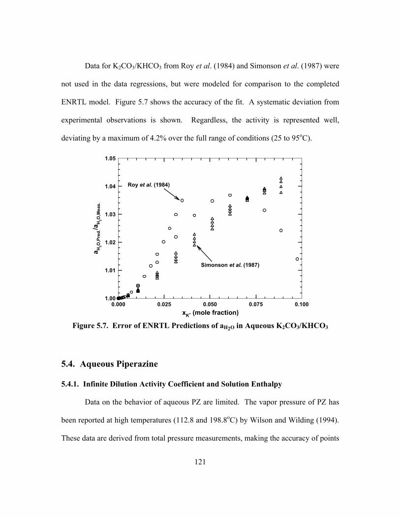
121
Data for K2CO3/KHCO3 from Roy et al. (1984) and Simonson et al. (1987) were
not used in the data regressions, but were modeled for comparison to the completed
ENRTL model. Figure 5.7 shows the accuracy of the fit. A systematic deviation from
experimental observations is shown. Regardless, the activity is represented well,
deviating by a maximum of 4.2% over the full range of conditions (25 to 95oC).
xK+ (mole fraction)0.000 0.025 0.050 0.075 0.100
a H2O
,Pre
d./a
H2O
,Mea
s.
1.00
1.01
1.02
1.03
1.04
1.05
Roy et al. (1984)
Simonson et al. (1987)
Figure 5.7. Error of ENRTL Predictions of aH2O in Aqueous K2CO3/KHCO3
5.4. Aqueous Piperazine
5.4.1. Infinite Dilution Activity Coefficient and Solution Enthalpy
Data on the behavior of aqueous PZ are limited. The vapor pressure of PZ has
been reported at high temperatures (112.8 and 198.8oC) by Wilson and Wilding (1994).
These data are derived from total pressure measurements, making the accuracy of points
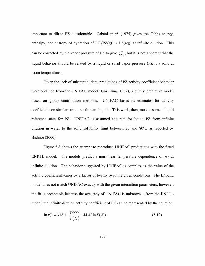
122
important to dilute PZ questionable. Cabani et al. (1975) gives the Gibbs energy,
enthalpy, and entropy of hydration of PZ (PZ(g) → PZ(aq)) at infinite dilution. This
can be corrected by the vapor pressure of PZ to give PZγ ∞ , but it is not apparent that the
liquid behavior should be related by a liquid or solid vapor pressure (PZ is a solid at
room temperature).
Given the lack of substantial data, predictions of PZ activity coefficient behavior
were obtained from the UNIFAC model (Gmehling, 1982), a purely predictive model
based on group contribution methods. UNIFAC bases its estimates for activity
coefficients on similar structures that are liquids. This work, then, must assume a liquid
reference state for PZ. UNIFAC is assumed accurate for liquid PZ from infinite
dilution in water to the solid solubility limit between 25 and 80oC as reported by
Bishnoi (2000).
Figure 5.8 shows the attempt to reproduce UNIFAC predictions with the fitted
ENRTL model. The models predict a non-linear temperature dependence of γPZ at
infinite dilution. The behavior suggested by UNIFAC is complex as the value of the
activity coefficient varies by a factor of twenty over the given conditions. The ENRTL
model does not match UNIFAC exactly with the given interaction parameters; however,
the fit is acceptable because the accuracy of UNIFAC is unknown. From the ENRTL
model, the infinite dilution activity coefficient of PZ can be represented by the equation
( ) ( )19779ln 318.1 44.42lnPZ T KT K
γ ∞ = − − . (5.12)
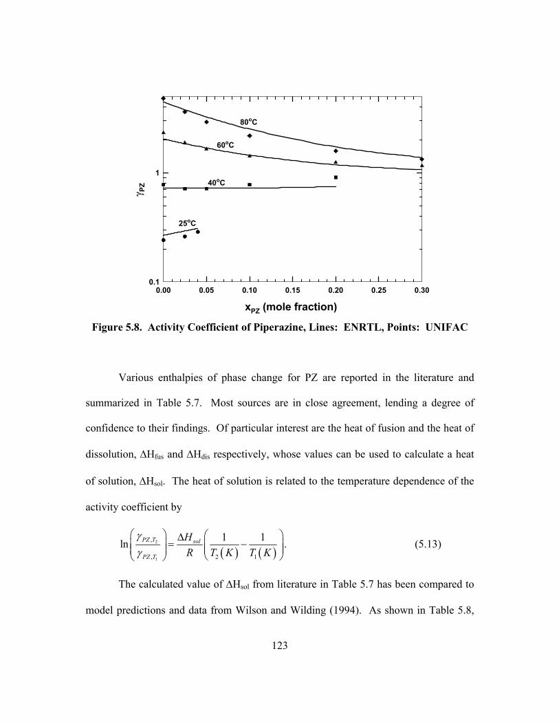
123
xPZ (mole fraction)0.00 0.05 0.10 0.15 0.20 0.25 0.30
γ PZ
0.1
1
80oC
25oC
40oC
60oC
Figure 5.8. Activity Coefficient of Piperazine, Lines: ENRTL, Points: UNIFAC
Various enthalpies of phase change for PZ are reported in the literature and
summarized in Table 5.7. Most sources are in close agreement, lending a degree of
confidence to their findings. Of particular interest are the heat of fusion and the heat of
dissolution, ∆Hfus and ∆Hdis respectively, whose values can be used to calculate a heat
of solution, ∆Hsol. The heat of solution is related to the temperature dependence of the
activity coefficient by
( ) ( )2
1
,
, 2 1
1 1ln PZ T sol
PZ T
HR T K T K
γγ
∆= −
. (5.13)
The calculated value of ∆Hsol from literature in Table 5.7 has been compared to
model predictions and data from Wilson and Wilding (1994). As shown in Table 5.8,
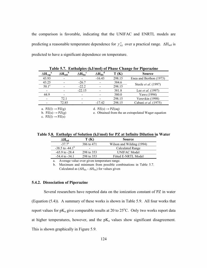
124
the comparison is favorable, indicating that the UNIFAC and ENRTL models are
predicting a reasonable temperature dependence for ∞PZγ over a practical range. ∆Hsol is
predicted to have a significant dependence on temperature.
Table 5.7. Enthalpies (kJ/mol) of Phase Change for Piperazine
∆Hvapa ∆Hsub
b ∆Hfusc ∆Hdis
d T (K) Source 43.93 - - -16.43 298.15 Enea and Berthon (1973) 43.25 - -26.7 - 384.6 50.1e - -22.2 - 298.15 Steele et al. (1997)
- - -22.15 - 381.8 Lee et al. (1997) 44.9 - - - 380.0 Yaws (1994)
- 72.1 - - 298.15 Verevkin (1998) - 72.85 - -17.42 298.15 Cabani et al. (1975)
Table 5.8. Enthalpy of Solution (kJ/mol) for PZ at Infinite Dilution in Water ∆Hsol
T (K) Source -37.7a 386 to 471 Wilson and Wilding (1994)
-38.5 to -44.1b - Calculated Range -65.9 to -28.4 298 to 353 UNIFAC Model -54.4 to -34.1 298 to 353 Fitted E-NRTL Model
a. Average value over given temperature range. b. Maximum and minimum from possible combinations in Table 5.7.
Calculated as (∆Hdis - ∆Hfus) for values given
5.4.2. Dissociation of Piperazine
Several researchers have reported data on the ionization constant of PZ in water
(Equation (5.4)). A summary of these works is shown in Table 5.9. All four works that
report values for pKa give comparable results at 20 to 25oC. Only two works report data
at higher temperatures, however, and the pKa values show significant disagreement.
This is shown graphically in Figure 5.9.
a. PZ(l) → PZ(g) d. PZ(s) → PZ(aq) b. PZ(s) → PZ(g) e. Obtained from the an extrapolated Wager equation c. PZ(l) → PZ(s)
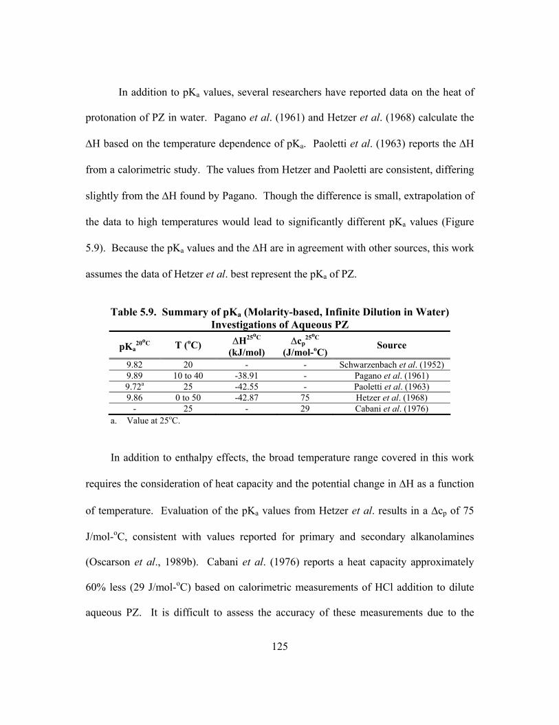
125
In addition to pKa values, several researchers have reported data on the heat of
protonation of PZ in water. Pagano et al. (1961) and Hetzer et al. (1968) calculate the
∆H based on the temperature dependence of pKa. Paoletti et al. (1963) reports the ∆H
from a calorimetric study. The values from Hetzer and Paoletti are consistent, differing
slightly from the ∆H found by Pagano. Though the difference is small, extrapolation of
the data to high temperatures would lead to significantly different pKa values (Figure
5.9). Because the pKa values and the ∆H are in agreement with other sources, this work
assumes the data of Hetzer et al. best represent the pKa of PZ.
Table 5.9. Summary of pKa (Molarity-based, Infinite Dilution in Water)
Investigations of Aqueous PZ
pKa20oC T (oC) ∆H25oC
(kJ/mol) ∆cp
25oC (J/mol-oC)
Source
9.82 20 - - Schwarzenbach et al. (1952) 9.89 10 to 40 -38.91 - Pagano et al. (1961) 9.72a 25 -42.55 - Paoletti et al. (1963) 9.86 0 to 50 -42.87 75 Hetzer et al. (1968)
- 25 - 29 Cabani et al. (1976) a. Value at 25oC.
In addition to enthalpy effects, the broad temperature range covered in this work
requires the consideration of heat capacity and the potential change in ∆H as a function
of temperature. Evaluation of the pKa values from Hetzer et al. results in a ∆cp of 75
J/mol-oC, consistent with values reported for primary and secondary alkanolamines
(Oscarson et al., 1989b). Cabani et al. (1976) reports a heat capacity approximately
60% less (29 J/mol-oC) based on calorimetric measurements of HCl addition to dilute
aqueous PZ. It is difficult to assess the accuracy of these measurements due to the
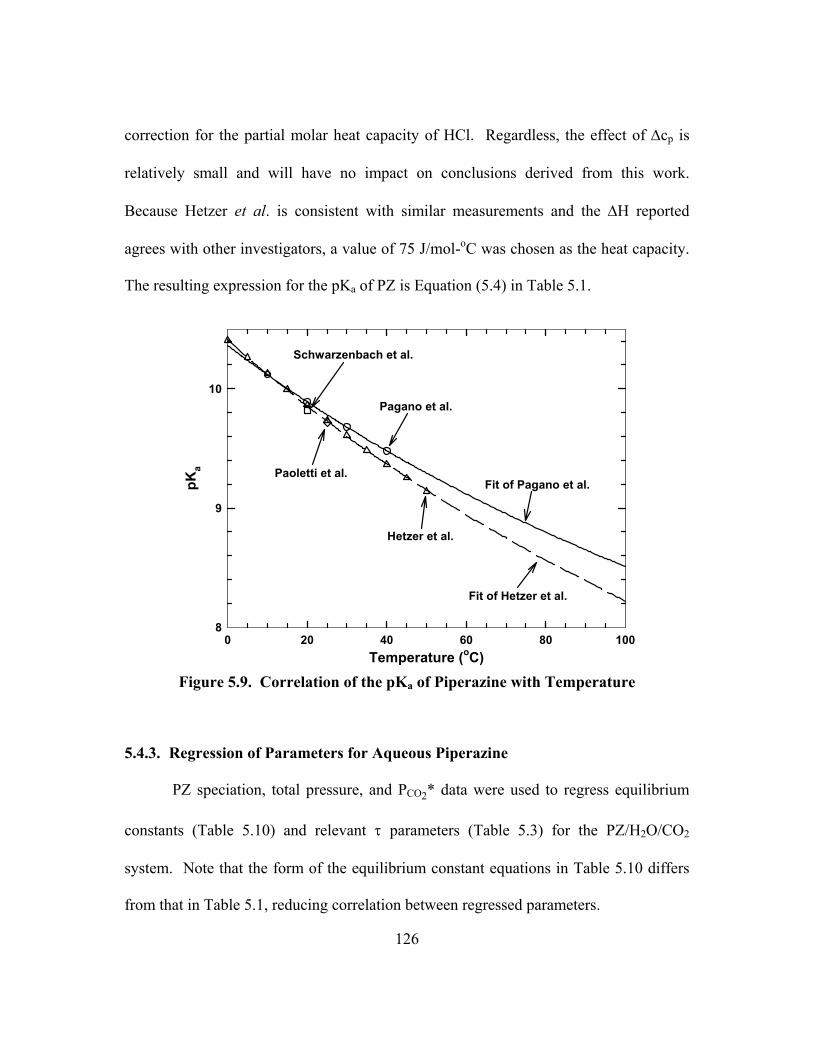
126
correction for the partial molar heat capacity of HCl. Regardless, the effect of ∆cp is
relatively small and will have no impact on conclusions derived from this work.
Because Hetzer et al. is consistent with similar measurements and the ∆H reported
agrees with other investigators, a value of 75 J/mol-oC was chosen as the heat capacity.
The resulting expression for the pKa of PZ is Equation (5.4) in Table 5.1.
Temperature (oC)0 20 40 60 80 100
pKa
8
9
10Pagano et al.
Hetzer et al.
Schwarzenbach et al.
Paoletti et al.Fit of Pagano et al.
Fit of Hetzer et al.
Figure 5.9. Correlation of the pKa of Piperazine with Temperature
5.4.3. Regression of Parameters for Aqueous Piperazine
PZ speciation, total pressure, and PCO2* data were used to regress equilibrium
constants (Table 5.10) and relevant τ parameters (Table 5.3) for the PZ/H2O/CO2
system. Note that the form of the equilibrium constant equations in Table 5.10 differs
from that in Table 5.1, reducing correlation between regressed parameters.
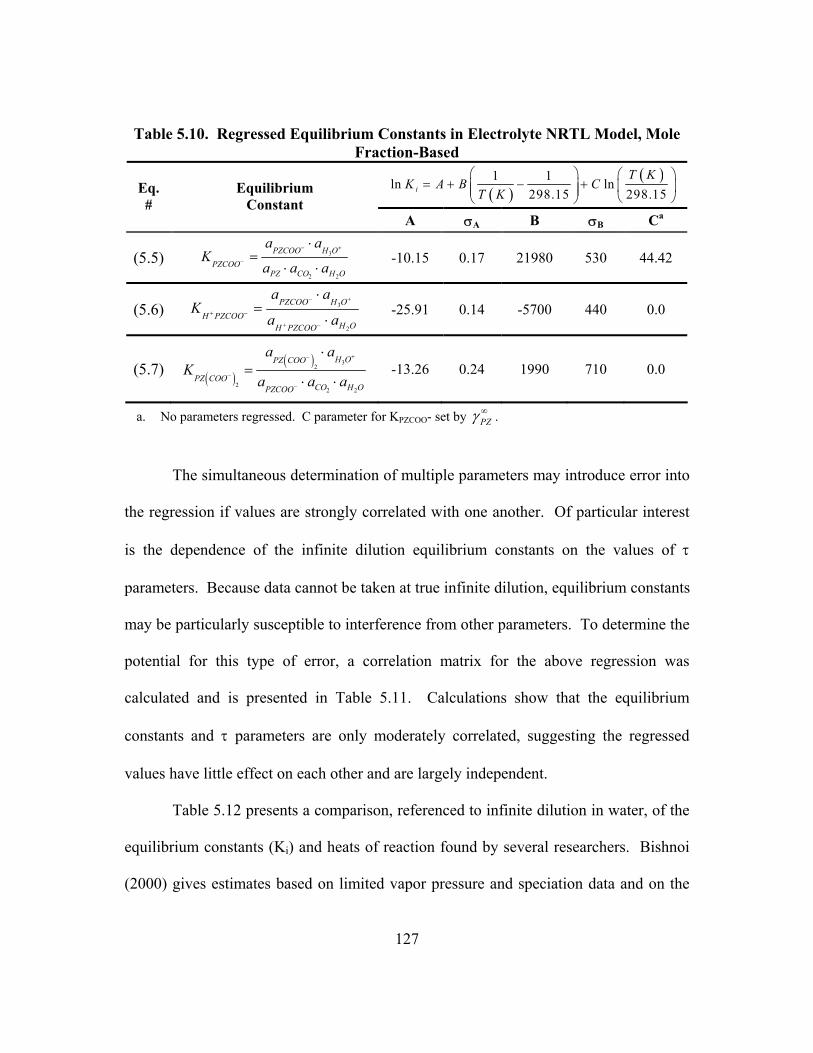
127
Table 5.10. Regressed Equilibrium Constants in Electrolyte NRTL Model, Mole Fraction-Based
( )( )1 1ln ln
298.15 298.15i
T KK A B C
T K
= + − + Eq.
# Equilibrium
Constant A σA B σB Ca
(5.5) 3
2 2
PZCOO H OPZCOO
PZ CO H O
a aK
a a a− +
−
⋅=
⋅ ⋅ -10.15 0.17 21980 530 44.42
(5.6) 3
2
PZCOO H OH PZCOO
H OH PZCOO
a aK
a a− +
+ −
+ −
⋅=
⋅ -25.91 0.14 -5700 440 0.0
(5.7) ( )( ) 3
2
22 2
H OPZ COO
PZ COOCO H OPZCOO
a aK
a a a
+−
−
−
⋅=
⋅ ⋅ -13.26 0.24 1990 710 0.0
a. No parameters regressed. C parameter for KPZCOO- set by PZγ ∞ .
The simultaneous determination of multiple parameters may introduce error into
the regression if values are strongly correlated with one another. Of particular interest
is the dependence of the infinite dilution equilibrium constants on the values of τ
parameters. Because data cannot be taken at true infinite dilution, equilibrium constants
may be particularly susceptible to interference from other parameters. To determine the
potential for this type of error, a correlation matrix for the above regression was
calculated and is presented in Table 5.11. Calculations show that the equilibrium
constants and τ parameters are only moderately correlated, suggesting the regressed
values have little effect on each other and are largely independent.
Table 5.12 presents a comparison, referenced to infinite dilution in water, of the
equilibrium constants (Ki) and heats of reaction found by several researchers. Bishnoi
(2000) gives estimates based on limited vapor pressure and speciation data and on the
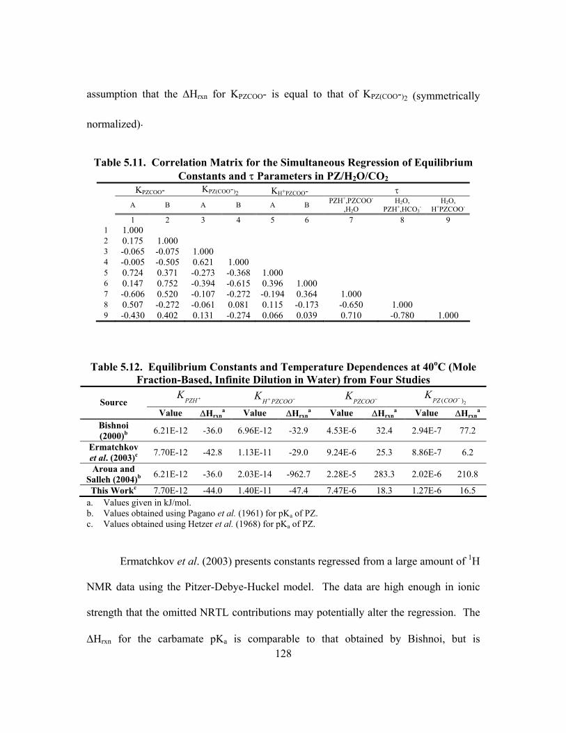
128
assumption that the ∆Hrxn for KPZCOO- is equal to that of KPZ(COO-)2 (symmetrically
normalized).
Table 5.11. Correlation Matrix for the Simultaneous Regression of Equilibrium
Constants and τ Parameters in PZ/H2O/CO2 KPZCOO- KPZ(COO-)2 KH+PZCOO- τ A B A B A B PZH+,PZCOO-
,H2O H2O,
PZH+,HCO3-
H2O, H+PZCOO-
1 2 3 4 5 6 7 8 9 1 1.000 2 0.175 1.000 3 -0.065 -0.075 1.000 4 -0.005 -0.505 0.621 1.000 5 0.724 0.371 -0.273 -0.368 1.000 6 0.147 0.752 -0.394 -0.615 0.396 1.000 7 -0.606 0.520 -0.107 -0.272 -0.194 0.364 1.000 8 0.507 -0.272 -0.061 0.081 0.115 -0.173 -0.650 1.000 9 -0.430 0.402 0.131 -0.274 0.066 0.039 0.710 -0.780 1.000
Table 5.12. Equilibrium Constants and Temperature Dependences at 40oC (Mole
Fraction-Based, Infinite Dilution in Water) from Four Studies
PZHK +
H PZCOOK + −
PZCOOK −
2( )PZ COOK −
Source Value ∆Hrxn
a Value ∆Hrxna Value ∆Hrxn
a Value ∆Hrxna
Bishnoi (2000)b 6.21E-12 -36.0 6.96E-12 -32.9 4.53E-6 32.4 2.94E-7 77.2
Ermatchkov et al. (2003)c 7.70E-12 -42.8 1.13E-11 -29.0 9.24E-6 25.3 8.86E-7 6.2
Aroua and Salleh (2004)b 6.21E-12 -36.0 2.03E-14 -962.7 2.28E-5 283.3 2.02E-6 210.8
This Workc 7.70E-12 -44.0 1.40E-11 -47.4 7.47E-6 18.3 1.27E-6 16.5 a. Values given in kJ/mol. b. Values obtained using Pagano et al. (1961) for pKa of PZ. c. Values obtained using Hetzer et al. (1968) for pKa of PZ.
Ermatchkov et al. (2003) presents constants regressed from a large amount of 1H
NMR data using the Pitzer-Debye-Huckel model. The data are high enough in ionic
strength that the omitted NRTL contributions may potentially alter the regression. The
∆Hrxn for the carbamate pKa is comparable to that obtained by Bishnoi, but is
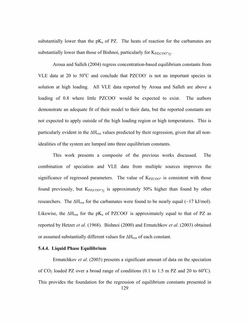
129
substantially lower than the pKa of PZ. The heats of reaction for the carbamates are
substantially lower than those of Bishnoi, particularly for KPZ(COO-)2.
Aroua and Salleh (2004) regress concentration-based equilibrium constants from
VLE data at 20 to 50oC and conclude that PZCOO- is not an important species in
solution at high loading. All VLE data reported by Aroua and Salleh are above a
loading of 0.8 where little PZCOO- would be expected to exist. The authors
demonstrate an adequate fit of their model to their data, but the reported constants are
not expected to apply outside of the high loading region or high temperatures. This is
particularly evident in the ∆Hrxn values predicted by their regression, given that all non-
idealities of the system are lumped into three equilibrium constants.
This work presents a composite of the previous works discussed. The
combination of speciation and VLE data from multiple sources improves the
significance of regressed parameters. The value of KPZCOO- is consistent with those
found previously, but KPZ(COO-)2 is approximately 50% higher than found by other
researchers. The ∆Hrxn for the carbamates were found to be nearly equal (~17 kJ/mol).
Likewise, the ∆Hrxn for the pKa of PZCOO- is approximately equal to that of PZ as
reported by Hetzer et al. (1968). Bishnoi (2000) and Ermatchkov et al. (2003) obtained
or assumed substantially different values for ∆Hrxn of each constant.
5.4.4. Liquid Phase Equilibrium
Ermatchkov et al. (2003) presents a significant amount of data on the speciation
of CO2 loaded PZ over a broad range of conditions (0.1 to 1.5 m PZ and 20 to 60oC).
This provides the foundation for the regression of equilibrium constants presented in
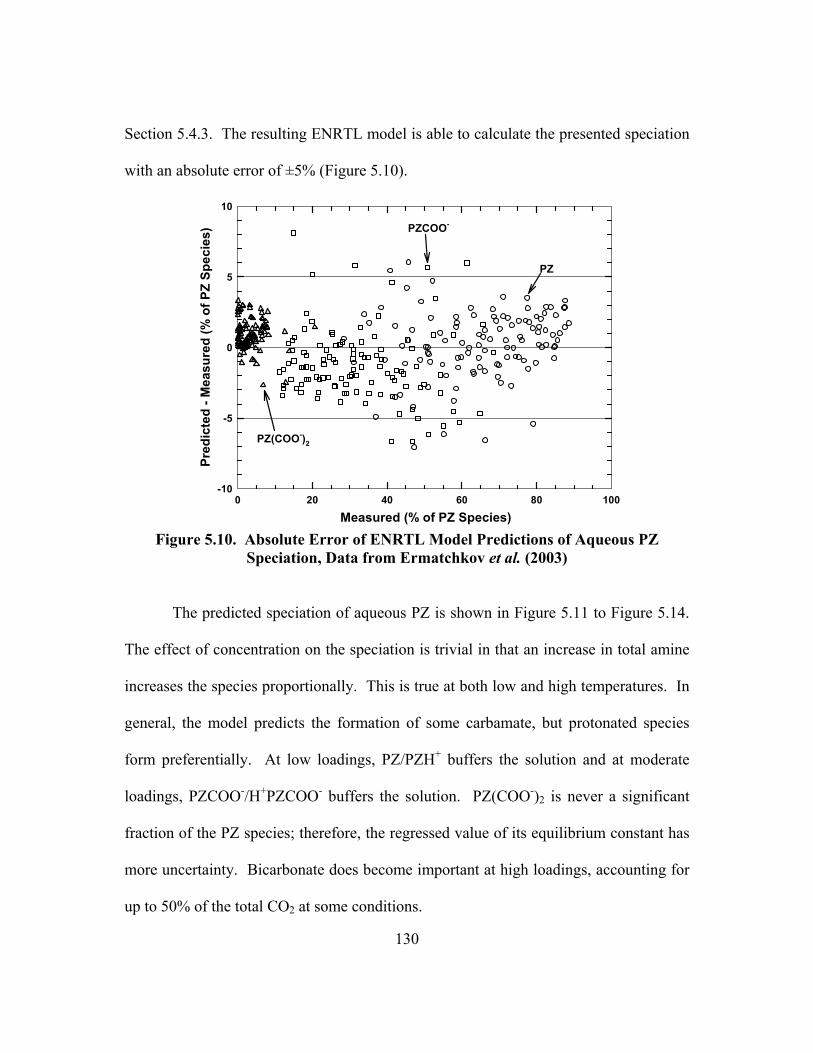
130
Section 5.4.3. The resulting ENRTL model is able to calculate the presented speciation
with an absolute error of ±5% (Figure 5.10).
Measured (% of PZ Species)0 20 40 60 80 100
Pred
icte
d - M
easu
red
(% o
f PZ
Spec
ies)
-10
-5
0
5
10
PZ
PZCOO-
PZ(COO-)2
Figure 5.10. Absolute Error of ENRTL Model Predictions of Aqueous PZ
Speciation, Data from Ermatchkov et al. (2003)
The predicted speciation of aqueous PZ is shown in Figure 5.11 to Figure 5.14.
The effect of concentration on the speciation is trivial in that an increase in total amine
increases the species proportionally. This is true at both low and high temperatures. In
general, the model predicts the formation of some carbamate, but protonated species
form preferentially. At low loadings, PZ/PZH+ buffers the solution and at moderate
loadings, PZCOO-/H+PZCOO- buffers the solution. PZ(COO-)2 is never a significant
fraction of the PZ species; therefore, the regressed value of its equilibrium constant has
more uncertainty. Bicarbonate does become important at high loadings, accounting for
up to 50% of the total CO2 at some conditions.

131
Loading (mol CO2/mol PZ)0.0 0.2 0.4 0.6 0.8 1.0
[Am
ine]
or [
CO
2 Spe
cies
] (m
)
0.01
0.1
1
P CO
2* (Pa
) or [
OH
- ] x 1
05 (m)
10
100
1000
10000PZ
PZCOO-
PZ(COO-)2
OH-
PZH+
H+PZCOO-
CO32-
HCO3-
PCO2*
Figure 5.11. Speciation in 0.6 m PZ at 60oC
Loading (mol CO2/mol PZ)0.0 0.2 0.4 0.6 0.8 1.0
[Am
ine]
or [
CO
2 Spe
cies
] (m
)
0.01
0.1
1
P CO
2* (Pa
) or [
OH
- ] x 1
05 (m)
10
100
1000
10000PZ
PZCOO-
PZ(COO-)2
OH-
PZH+
H+PZCOO-
HCO3-
PCO2*
Figure 5.12. Speciation in 0.6 m PZ at 110oC
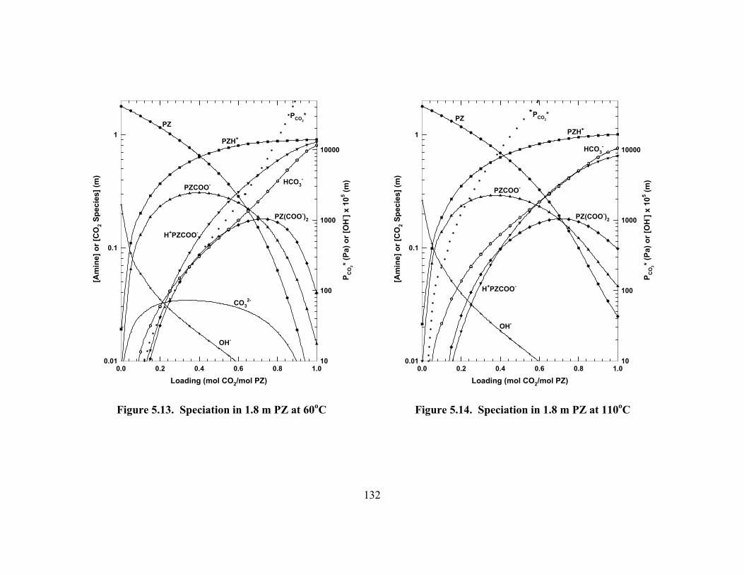
132
Loading (mol CO2/mol PZ)0.0 0.2 0.4 0.6 0.8 1.0
[Am
ine]
or [
CO
2 Spe
cies
] (m
)
0.01
0.1
1
P CO
2* (Pa
) or [
OH
- ] x 1
05 (m)
10
100
1000
10000
PZ
PZCOO-
PZ(COO-)2
OH-
PZH+
H+PZCOO-
CO32-
HCO3-
PCO2*
Figure 5.13. Speciation in 1.8 m PZ at 60oC
Loading (mol CO2/mol PZ)0.0 0.2 0.4 0.6 0.8 1.0
[Am
ine]
or [
CO
2 Spe
cies
] (m
)
0.01
0.1
1
P CO
2* (Pa
) or [
OH
- ] x 1
05 (m)
10
100
1000
10000
PZ
PZCOO-
PZ(COO-)2
OH-
PZH+
H+PZCOO-
HCO3-
PCO2*
Figure 5.14. Speciation in 1.8 m PZ at 110oC
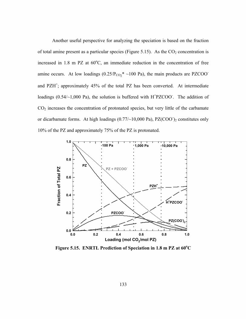
133
Another useful perspective for analyzing the speciation is based on the fraction
of total amine present as a particular species (Figure 5.15). As the CO2 concentration is
increased in 1.8 m PZ at 60oC, an immediate reduction in the concentration of free
amine occurs. At low loadings (0.25/PCO2* ~100 Pa), the main products are PZCOO-
and PZH+; approximately 45% of the total PZ has been converted. At intermediate
loadings (0.54/~1,000 Pa), the solution is buffered with H+PZCOO-. The addition of
CO2 increases the concentration of protonated species, but very little of the carbamate
or dicarbamate forms. At high loadings (0.77/~10,000 Pa), PZ(COO-)2 constitutes only
10% of the PZ and approximately 75% of the PZ is protonated.
Loading (mol CO2/mol PZ)0.0 0.2 0.4 0.6 0.8 1.0
Frac
tion
of T
otal
PZ
0.0
0.2
0.4
0.6
0.8
1.0
PZ
H+PZCOO-
PZH+
PZ(COO-)2
PZCOO-
PZ + PZCOO-
100 Pa 1,000 Pa 10,000 Pa
Figure 5.15. ENRTL Prediction of Speciation in 1.8 m PZ at 60oC
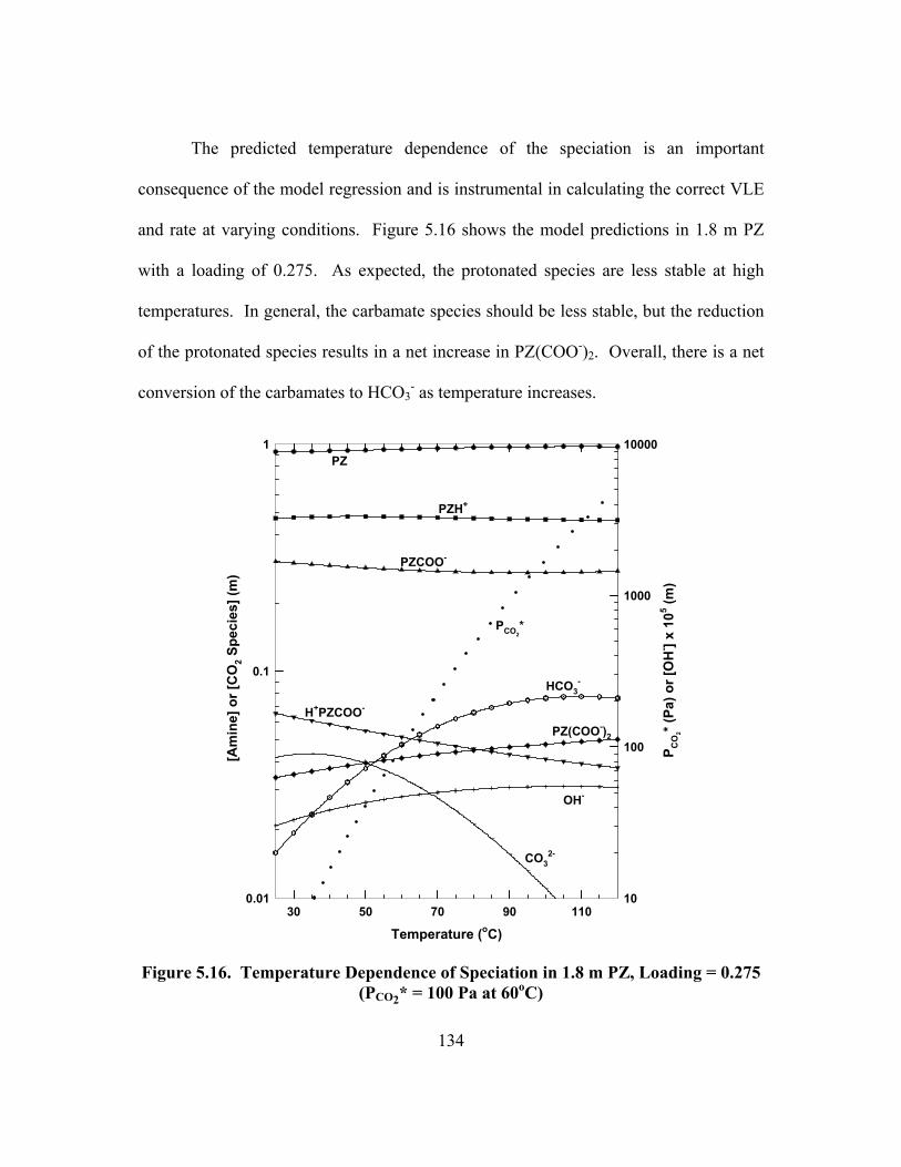
134
The predicted temperature dependence of the speciation is an important
consequence of the model regression and is instrumental in calculating the correct VLE
and rate at varying conditions. Figure 5.16 shows the model predictions in 1.8 m PZ
with a loading of 0.275. As expected, the protonated species are less stable at high
temperatures. In general, the carbamate species should be less stable, but the reduction
of the protonated species results in a net increase in PZ(COO-)2. Overall, there is a net
conversion of the carbamates to HCO3- as temperature increases.
Temperature (oC)30 50 70 90 110
[Am
ine]
or [
CO
2 Spe
cies
] (m
)
0.01
0.1
1
P CO
2* (Pa
) or [
OH
- ] x 1
05 (m)
10
100
1000
10000PZ
PZCOO-
PZ(COO-)2
OH-
PZH+
H+PZCOO-
CO32-
HCO3-
PCO2*
Figure 5.16. Temperature Dependence of Speciation in 1.8 m PZ, Loading = 0.275
(PCO2* = 100 Pa at 60oC)
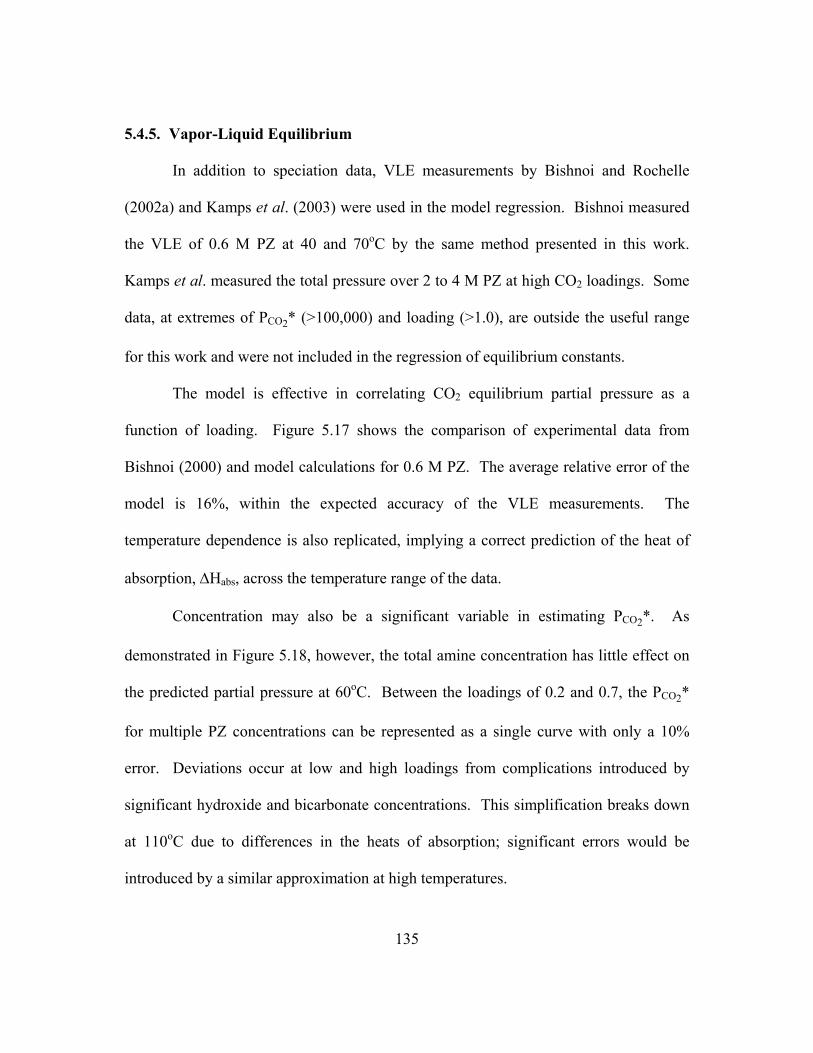
135
5.4.5. Vapor-Liquid Equilibrium
In addition to speciation data, VLE measurements by Bishnoi and Rochelle
(2002a) and Kamps et al. (2003) were used in the model regression. Bishnoi measured
the VLE of 0.6 M PZ at 40 and 70oC by the same method presented in this work.
Kamps et al. measured the total pressure over 2 to 4 M PZ at high CO2 loadings. Some
data, at extremes of PCO2* (>100,000) and loading (>1.0), are outside the useful range
for this work and were not included in the regression of equilibrium constants.
The model is effective in correlating CO2 equilibrium partial pressure as a
function of loading. Figure 5.17 shows the comparison of experimental data from
Bishnoi (2000) and model calculations for 0.6 M PZ. The average relative error of the
model is 16%, within the expected accuracy of the VLE measurements. The
temperature dependence is also replicated, implying a correct prediction of the heat of
absorption, ∆Habs, across the temperature range of the data.
Concentration may also be a significant variable in estimating PCO2*. As
demonstrated in Figure 5.18, however, the total amine concentration has little effect on
the predicted partial pressure at 60oC. Between the loadings of 0.2 and 0.7, the PCO2*
for multiple PZ concentrations can be represented as a single curve with only a 10%
error. Deviations occur at low and high loadings from complications introduced by
significant hydroxide and bicarbonate concentrations. This simplification breaks down
at 110oC due to differences in the heats of absorption; significant errors would be
introduced by a similar approximation at high temperatures.
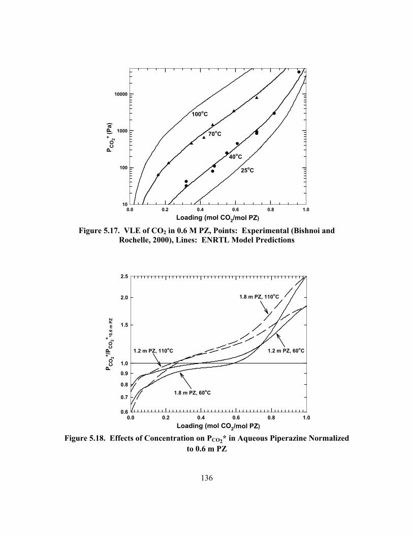
136
Loading (mol CO2/mol PZ)0.0 0.2 0.4 0.6 0.8 1.0
P CO
2* (Pa
)
10
100
1000
10000
70oC
40oC
100oC
25oC
Figure 5.17. VLE of CO2 in 0.6 M PZ, Points: Experimental (Bishnoi and
Rochelle, 2000), Lines: ENRTL Model Predictions
Loading (mol CO2/mol PZ)0.0 0.2 0.4 0.6 0.8 1.0
P CO
2*/PC
O2*, 0.
6 m
PZ
0.6
0.7
0.8
0.9
1.5
2.0
2.5
1.0
1.8 m PZ, 60oC
1.2 m PZ, 60oC
1.8 m PZ, 110oC
1.2 m PZ, 110oC
Figure 5.18. Effects of Concentration on PCO2* in Aqueous Piperazine Normalized
to 0.6 m PZ
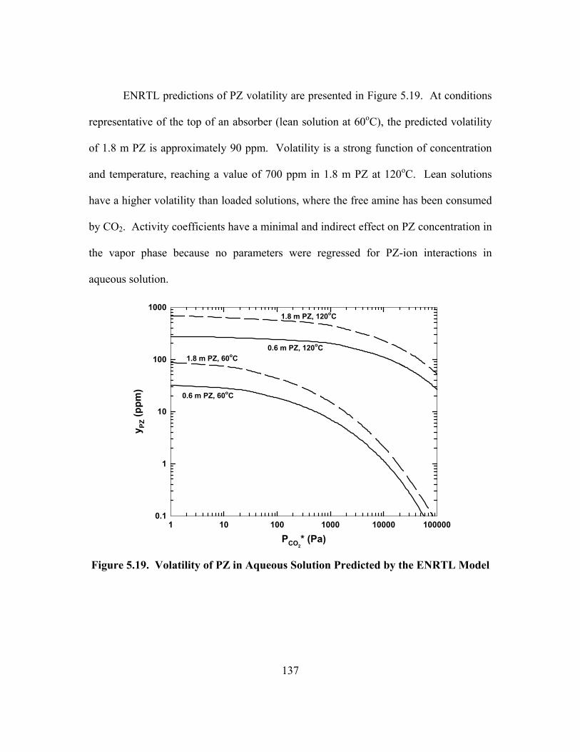
137
ENRTL predictions of PZ volatility are presented in Figure 5.19. At conditions
representative of the top of an absorber (lean solution at 60oC), the predicted volatility
of 1.8 m PZ is approximately 90 ppm. Volatility is a strong function of concentration
and temperature, reaching a value of 700 ppm in 1.8 m PZ at 120oC. Lean solutions
have a higher volatility than loaded solutions, where the free amine has been consumed
by CO2. Activity coefficients have a minimal and indirect effect on PZ concentration in
the vapor phase because no parameters were regressed for PZ-ion interactions in
aqueous solution.
PCO2* (Pa)
1 10 100 1000 10000 100000
y PZ (p
pm)
0.1
1
10
100
10001.8 m PZ, 120oC
0.6 m PZ, 60oC
1.8 m PZ, 60oC0.6 m PZ, 120oC
Figure 5.19. Volatility of PZ in Aqueous Solution Predicted by the ENRTL Model
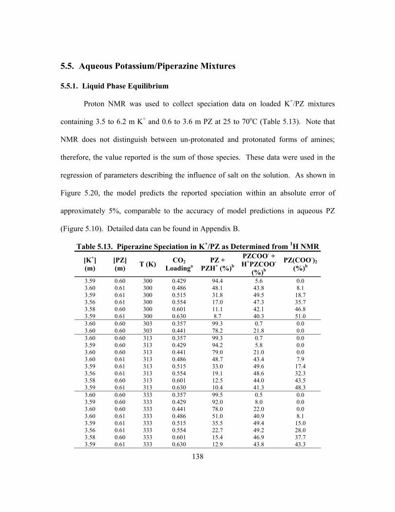
138
5.5. Aqueous Potassium/Piperazine Mixtures
5.5.1. Liquid Phase Equilibrium
Proton NMR was used to collect speciation data on loaded K+/PZ mixtures
containing 3.5 to 6.2 m K+ and 0.6 to 3.6 m PZ at 25 to 70oC (Table 5.13). Note that
NMR does not distinguish between un-protonated and protonated forms of amines;
therefore, the value reported is the sum of those species. These data were used in the
regression of parameters describing the influence of salt on the solution. As shown in
Figure 5.20, the model predicts the reported speciation within an absolute error of
approximately 5%, comparable to the accuracy of model predictions in aqueous PZ
(Figure 5.10). Detailed data can be found in Appendix B.
Table 5.13. Piperazine Speciation in K+/PZ as Determined from 1H NMR
[K+] (m)
[PZ] (m) T (K) CO2
Loadinga PZ +
PZH+ (%)b
PZCOO- + H+PZCOO-
(%)b
PZ(COO-)2 (%)b
3.59 0.60 300 0.429 94.4 5.6 0.0 3.60 0.61 300 0.486 48.1 43.8 8.1 3.59 0.61 300 0.515 31.8 49.5 18.7 3.56 0.61 300 0.554 17.0 47.3 35.7 3.58 0.60 300 0.601 11.1 42.1 46.8 3.59 0.61 300 0.630 8.7 40.3 51.0 3.60 0.60 303 0.357 99.3 0.7 0.0 3.60 0.60 303 0.441 78.2 21.8 0.0 3.60 0.60 313 0.357 99.3 0.7 0.0 3.59 0.60 313 0.429 94.2 5.8 0.0 3.60 0.60 313 0.441 79.0 21.0 0.0 3.60 0.61 313 0.486 48.7 43.4 7.9 3.59 0.61 313 0.515 33.0 49.6 17.4 3.56 0.61 313 0.554 19.1 48.6 32.3 3.58 0.60 313 0.601 12.5 44.0 43.5 3.59 0.61 313 0.630 10.4 41.3 48.3 3.60 0.60 333 0.357 99.5 0.5 0.0 3.59 0.60 333 0.429 92.0 8.0 0.0 3.60 0.60 333 0.441 78.0 22.0 0.0 3.60 0.61 333 0.486 51.0 40.9 8.1 3.59 0.61 333 0.515 35.5 49.4 15.0 3.56 0.61 333 0.554 22.7 49.2 28.0 3.58 0.60 333 0.601 15.4 46.9 37.7 3.59 0.61 333 0.630 12.9 43.8 43.3

139
[K+] (m)
[PZ] (m) T (K) CO2
Loadinga PZ +
PZH+ (%)b
PZCOO- + H+PZCOO-
(%)b
PZ(COO-)2 (%)b
3.59 0.60 343 0.429 91.0 9.0 0.0 3.60 0.61 343 0.486 52.1 41.2 6.7 3.59 0.61 343 0.515 37.6 49.3 13.1 3.59 1.81 300 0.433 51.5 41.0 7.5 3.44 1.85 303 0.618 17.3 47.0 35.7 3.46 1.86 303 0.694 9.5 62.4 28.1 3.59 1.81 313 0.433 51.6 41.4 6.9 3.44 1.85 313 0.618 18.1 47.5 34.4 3.46 1.86 313 0.694 11.4 61.2 27.3 3.59 1.81 333 0.433 52.2 41.3 6.5 3.44 1.85 333 0.618 20.4 47.0 32.6 3.57 3.58 300 0.499 35.4 49.0 15.6 3.59 3.61 300 0.600 20.2 48.6 31.2 3.59 3.59 300 0.646 26.0 49.1 24.9 3.60 3.58 313 0.376 59.2 36.5 4.2 3.57 3.58 313 0.499 35.3 48.8 15.8 3.59 3.61 313 0.600 21.2 48.8 29.9 3.59 3.59 313 0.646 25.9 49.6 24.5 3.60 3.58 333 0.376 59.5 36.6 3.9 3.57 3.58 333 0.499 36.0 48.6 15.4 3.59 3.59 333 0.646 28.1 47.6 24.3 5.00 2.50 300 0.433 76.3 22.5 1.2 4.99 2.51 300 0.467 43.9 46.8 9.2 4.64 2.50 300 0.650 11.5 43.8 44.7 4.98 2.50 300 0.534 27.9 50.4 21.6 4.98 2.50 300 0.600 14.9 46.5 38.7 5.00 2.50 313 0.433 69.8 28.1 2.1 4.99 2.51 313 0.467 44.0 47.2 8.8 4.64 2.50 313 0.650 12.3 44.3 43.4 4.98 2.50 313 0.534 27.5 50.2 22.3 4.98 2.50 313 0.600 15.2 46.1 38.8 5.00 2.50 333 0.433 53.6 40.0 6.4 4.99 2.51 333 0.467 42.0 46.5 11.5 4.64 2.50 333 0.650 15.2 43.2 41.6 4.98 2.50 333 0.534 25.1 54.7 20.2 4.98 2.50 333 0.600 15.8 49.3 34.9 6.18 1.23 300 0.570 16.0 46.4 37.6 6.18 1.23 313 0.570 13.2 45.7 41.2 6.18 1.23 333 0.570 14.5 47.6 37.8 6.20 1.81 300 0.666 12.4 44.7 42.9 6.21 1.81 313 0.527 36.1 48.7 15.2 6.20 1.81 313 0.666 13.2 45.8 41.1 6.21 1.81 333 0.527 36.9 49.0 14.2 6.20 1.81 333 0.666 15.0 48.2 36.8 a. Loading = mol CO2,TOT/(mol PZ + mol K+). b. Values reported as % of total PZ.
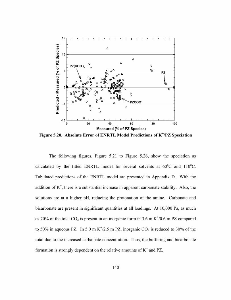
140
Measured (% of PZ Species)0 20 40 60 80 100
Pred
icte
d - M
easu
red
(% o
f PZ
Spec
ies)
-10
-5
0
5
10
15
PZ
PZCOO-
PZ(COO-)2
Figure 5.20. Absolute Error of ENRTL Model Predictions of K+/PZ Speciation
The following figures, Figure 5.21 to Figure 5.26, show the speciation as
calculated by the fitted ENRTL model for several solvents at 60oC and 110oC.
Tabulated predictions of the ENRTL model are presented in Appendix D. With the
addition of K+, there is a substantial increase in apparent carbamate stability. Also, the
solutions are at a higher pH, reducing the protonation of the amine. Carbonate and
bicarbonate are present in significant quantities at all loadings. At 10,000 Pa, as much
as 70% of the total CO2 is present in an inorganic form in 3.6 m K+/0.6 m PZ compared
to 50% in aqueous PZ. In 5.0 m K+/2.5 m PZ, inorganic CO2 is reduced to 30% of the
total due to the increased carbamate concentration. Thus, the buffering and bicarbonate
formation is strongly dependent on the relative amounts of K+ and PZ.
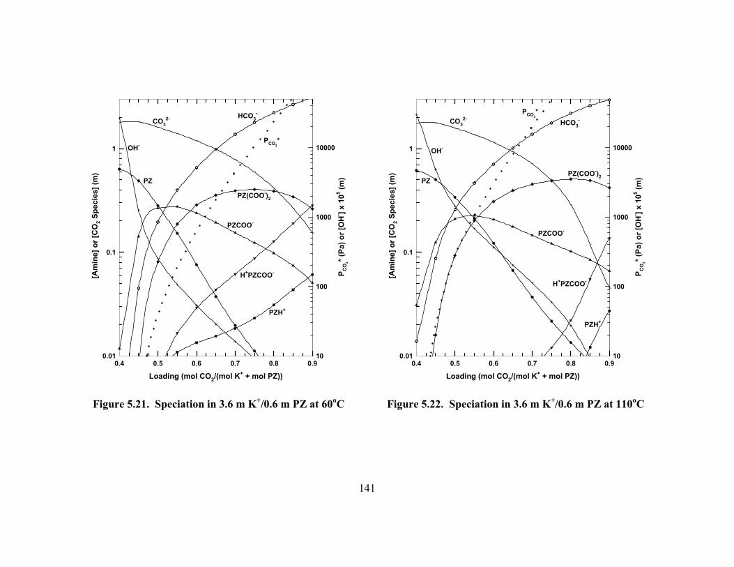
141
Loading (mol CO2/(mol K+ + mol PZ))0.4 0.5 0.6 0.7 0.8 0.9
[Am
ine]
or [
CO
2 Spe
cies
] (m
)
0.01
0.1
1
P CO
2* (Pa
) or [
OH
- ] x 1
05 (m)
10
100
1000
10000
PZ
PZCOO-
PZ(COO-)2
OH-
PZH+
H+PZCOO-
CO32- HCO3
-
PCO2*
Figure 5.21. Speciation in 3.6 m K+/0.6 m PZ at 60oC
Loading (mol CO2/(mol K+ + mol PZ))0.4 0.5 0.6 0.7 0.8 0.9
[Am
ine]
or [
CO
2 Spe
cies
] (m
)
0.01
0.1
1
P CO
2* (Pa
) or [
OH
- ] x 1
05 (m)
10
100
1000
10000
PZ
PZCOO-
PZ(COO-)2
OH-
PZH+
H+PZCOO-
CO32-
HCO3-
PCO2*
Figure 5.22. Speciation in 3.6 m K+/0.6 m PZ at 110oC
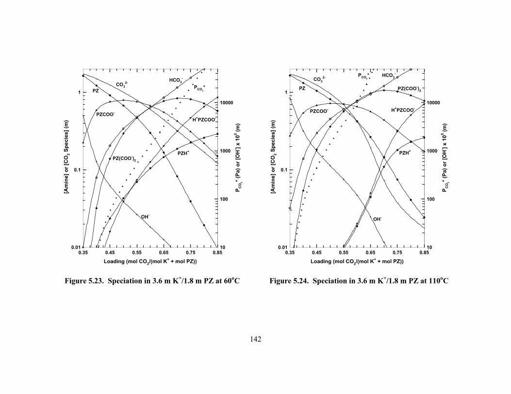
142
Loading (mol CO2/(mol K+ + mol PZ))0.35 0.45 0.55 0.65 0.75 0.85
[Am
ine]
or [
CO
2 Spe
cies
] (m
)
0.01
0.1
1
P CO
2* (Pa
) or [
OH
- ] x 1
05 (m)
10
100
1000
10000
PZ
PZCOO-
PZ(COO-)2
OH-
PZH+
H+PZCOO-
HCO3-
PCO2*CO3
2-
Figure 5.23. Speciation in 3.6 m K+/1.8 m PZ at 60oC
Loading (mol CO2/(mol K+ + mol PZ))0.35 0.45 0.55 0.65 0.75 0.85
[Am
ine]
or [
CO
2 Spe
cies
] (m
)
0.01
0.1
1
P CO
2* (Pa
) or [
OH
- ] x 1
05 (m)
10
100
1000
10000
PZ
PZCOO-
PZ(COO-)2
OH-
PZH+
H+PZCOO-
HCO3-PCO2
*CO3
2-
Figure 5.24. Speciation in 3.6 m K+/1.8 m PZ at 110oC
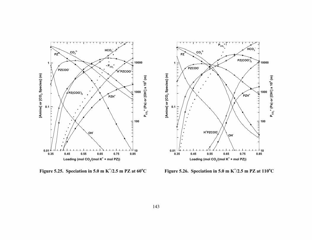
143
Loading (mol CO2/(mol K+ + mol PZ))0.35 0.45 0.55 0.65 0.75 0.85
[Am
ine]
or [
CO
2 Spe
cies
] (m
)
0.01
0.1
1
P CO
2* (Pa
) or [
OH
- ] x 1
05 (m)
10
100
1000
10000
PZ
PZCOO-
PZ(COO-)2
OH-
PZH+
H+PZCOO-
CO32- HCO3
-
PCO2*
Figure 5.25. Speciation in 5.0 m K+/2.5 m PZ at 60oC
Loading (mol CO2/(mol K+ + mol PZ))0.35 0.45 0.55 0.65 0.75 0.85
[Am
ine]
or [
CO
2 Spe
cies
] (m
)
0.01
0.1
1
P CO
2* (Pa
) or [
OH
- ] x 1
05 (m)
10
100
1000
10000
PZ
PZCOO-
PZ(COO-)2
OH-
PZH+
H+PZCOO-
CO32-
HCO3-
PCO2*
Figure 5.26. Speciation in 5.0 m K+/2.5 m PZ at 110oC
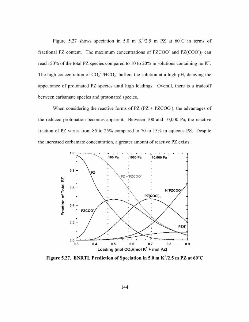
144
Figure 5.27 shows speciation in 5.0 m K+/2.5 m PZ at 60oC in terms of
fractional PZ content. The maximum concentrations of PZCOO- and PZ(COO-)2 can
reach 50% of the total PZ species compared to 10 to 20% in solutions containing no K+.
The high concentration of CO32-/HCO3
- buffers the solution at a high pH, delaying the
appearance of protonated PZ species until high loadings. Overall, there is a tradeoff
between carbamate species and protonated species.
When considering the reactive forms of PZ (PZ + PZCOO-), the advantages of
the reduced protonation becomes apparent. Between 100 and 10,000 Pa, the reactive
fraction of PZ varies from 85 to 25% compared to 70 to 15% in aqueous PZ. Despite
the increased carbamate concentration, a greater amount of reactive PZ exists.
Loading (mol CO2/(mol K+ + mol PZ)0.3 0.4 0.5 0.6 0.7 0.8 0.9
Frac
tion
of T
otal
PZ
0.0
0.2
0.4
0.6
0.8
1.0
PZ
H+PZCOO-
PZH+
PZ(COO-)2
PZCOO-
PZ + PZCOO-
100 Pa 1000 Pa 10,000 Pa
Figure 5.27. ENRTL Prediction of Speciation in 5.0 m K+/2.5 m PZ at 60oC
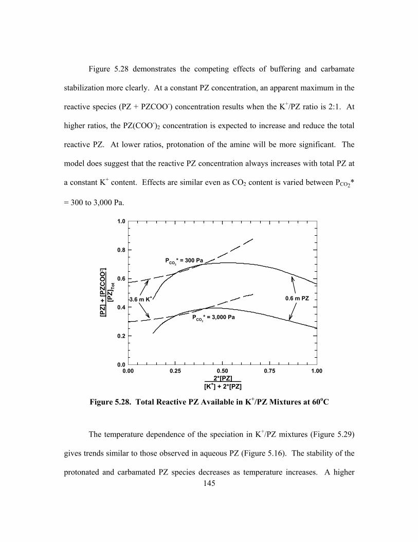
145
Figure 5.28 demonstrates the competing effects of buffering and carbamate
stabilization more clearly. At a constant PZ concentration, an apparent maximum in the
reactive species (PZ + PZCOO-) concentration results when the K+/PZ ratio is 2:1. At
higher ratios, the PZ(COO-)2 concentration is expected to increase and reduce the total
reactive PZ. At lower ratios, protonation of the amine will be more significant. The
model does suggest that the reactive PZ concentration always increases with total PZ at
a constant K+ content. Effects are similar even as CO2 content is varied between PCO2*
= 300 to 3,000 Pa.
2*[PZ] [K+] + 2*[PZ]
0.00 0.25 0.50 0.75 1.00
[PZ]
+ [P
ZCO
O- ]
[PZ]
Tot
0.0
0.2
0.4
0.6
0.8
1.0
0.6 m PZ3.6 m K+
PCO2* = 300 Pa
PCO2* = 3,000 Pa
Figure 5.28. Total Reactive PZ Available in K+/PZ Mixtures at 60oC
The temperature dependence of the speciation in K+/PZ mixtures (Figure 5.29)
gives trends similar to those observed in aqueous PZ (Figure 5.16). The stability of the
protonated and carbamated PZ species decreases as temperature increases. A higher
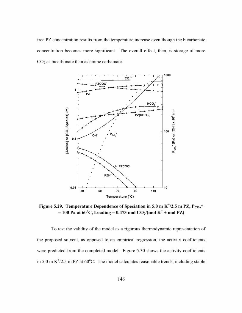
146
free PZ concentration results from the temperature increase even though the bicarbonate
concentration becomes more significant. The overall effect, then, is storage of more
CO2 as bicarbonate than as amine carbamate.
Temperature (oC)30 50 70 90 110
[Am
ine]
or [
CO
2 Spe
cies
] (m
)
0.01
0.1
1
P CO
2* (Pa
) or [
OH
- ] x 1
05 (m)
10
100
1000
PZ
PZCOO-
PZ(COO-)2
OH-
PZH+
H+PZCOO-
CO32-
HCO3-
PCO2*
Figure 5.29. Temperature Dependence of Speciation in 5.0 m K+/2.5 m PZ, PCO2*
= 100 Pa at 60oC, Loading = 0.473 mol CO2/(mol K+ + mol PZ)
To test the validity of the model as a rigorous thermodynamic representation of
the proposed solvent, as opposed to an empirical regression, the activity coefficients
were predicted from the completed model. Figure 5.30 shows the activity coefficients
in 5.0 m K+/2.5 m PZ at 60oC. The model calculates reasonable trends, including stable
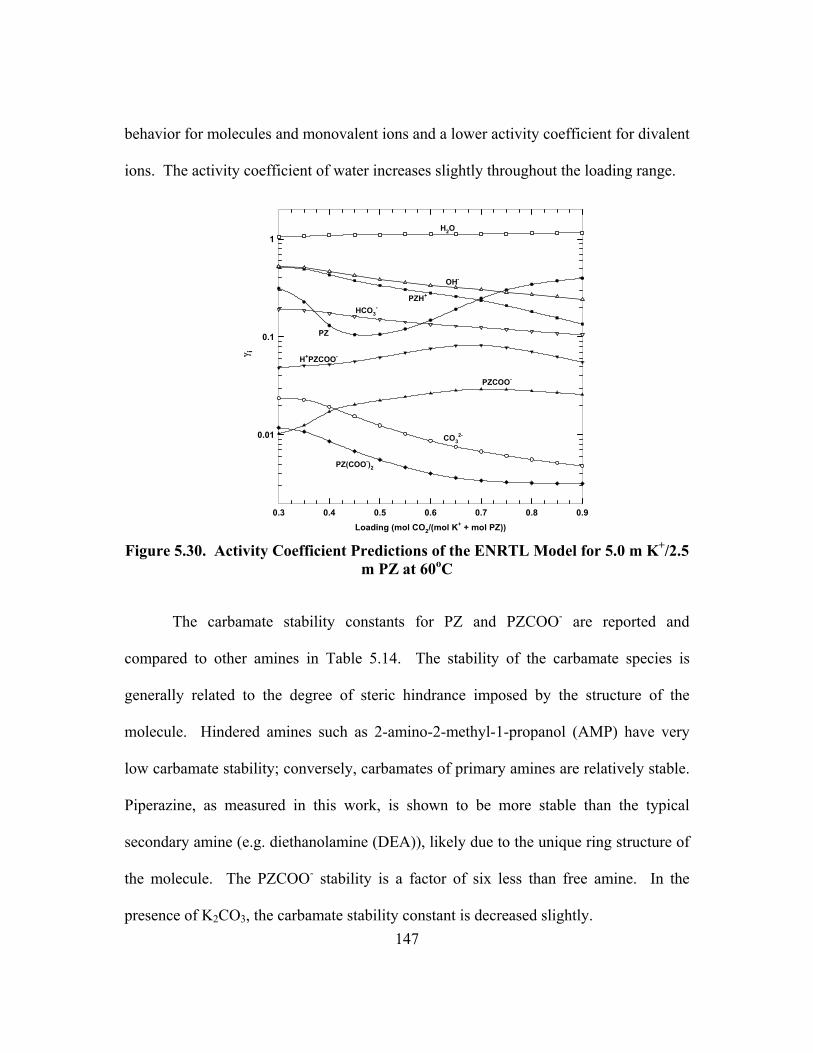
147
behavior for molecules and monovalent ions and a lower activity coefficient for divalent
ions. The activity coefficient of water increases slightly throughout the loading range.
Loading (mol CO2/(mol K+ + mol PZ))0.3 0.4 0.5 0.6 0.7 0.8 0.9
γ i
0.01
0.1
1
PZ
PZCOO-
PZ(COO-)2
OH-
PZH+
H+PZCOO-
CO32-
HCO3-
H2O
Figure 5.30. Activity Coefficient Predictions of the ENRTL Model for 5.0 m K+/2.5
m PZ at 60oC
The carbamate stability constants for PZ and PZCOO- are reported and
compared to other amines in Table 5.14. The stability of the carbamate species is
generally related to the degree of steric hindrance imposed by the structure of the
molecule. Hindered amines such as 2-amino-2-methyl-1-propanol (AMP) have very
low carbamate stability; conversely, carbamates of primary amines are relatively stable.
Piperazine, as measured in this work, is shown to be more stable than the typical
secondary amine (e.g. diethanolamine (DEA)), likely due to the unique ring structure of
the molecule. The PZCOO- stability is a factor of six less than free amine. In the
presence of K2CO3, the carbamate stability constant is decreased slightly.

148
Table 5.14. Comparison of Concentration-based (Molarity) Carbamate Stability
Constants at 40oC Amine Structure Environment Kcarb
a Source
xMEA → 0 45.5 Austgen (1989) MEA OH CH2 CH2 N
H
H
xMEA → 0 12.5 Sartori and Savage (1983)
AMP OH CH2 C NH
H
CH3
CH3
xAMP → 0 < 0.1 Sartori and Savage
(1983)
xDEA → 0 2.0 Austgen (1989) DEA
OH CH2 CH2
OH CH2 CH2
N H
4 M MDEA 0.1 Bishnoi (2000) xPZ → 0 10.1
4 M MDEA 13.2 Bishnoi (2000)
xPZ → 0 15.6 PZ NHCH2
CH2
NHCH2
CH2
2.5 m K2CO3 16.1 This Work
xPZ → 0 0.5 4 M MDEA 8.0
Bishnoi (2000)
xPZ → 0 2.7 PZCOO- NHCH2
CH2
NCH2
CH2
CO
O
2.5 m K2CO3 2.8 This Work
a. [ ] 3
carb
AmCOOK
Am HCO
−
−
=
5.5.2. Vapor-Liquid Equilibrium
In addition to speciation data, vapor pressure of CO2 over the mixed solvent
system (2.5 to 6.2 m K+ and 0.0 to 3.6 m PZ) was measured using the wetted-wall
column. Data from 40 to 110oC are shown in Table 5.15 as well as model predictions.
The data were used, in conjunction with the NMR speciation, to regress K+-PZ
interaction parameters. Detailed data are presented in Appendix C. Detailed model
predictions are shown in Appendix D.
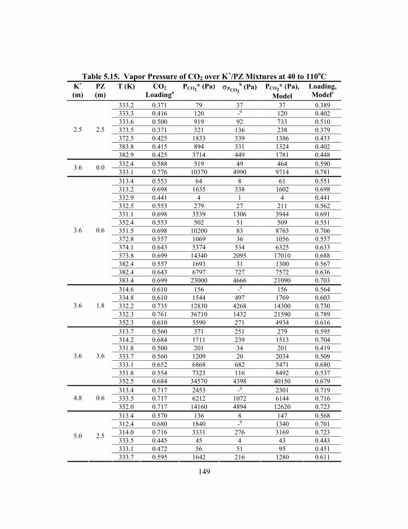
149
Table 5.15. Vapor Pressure of CO2 over K+/PZ Mixtures at 40 to 110oC
K+ (m)
PZ (m)
T (K) CO2 Loadinga
PCO2* (Pa) σPCO2b (Pa) PCO2* (Pa),
Model Loading, Modelc
333.2 0.371 79 37 37 0.389 333.3 0.416 120 -d 120 0.402 333.6 0.500 919 92 733 0.510 373.5 0.371 321 136 238 0.379 372.5 0.425 1833 339 1386 0.433 383.8 0.415 894 331 1324 0.402
2.5 2.5
382.9 0.425 3714 449 1781 0.448 332.4 0.588 519 49 464 0.590 3.6 0.0 333.1 0.776 10370 4990 9714 0.781 313.4 0.553 64 8 61 0.551 313.2 0.698 1635 338 1602 0.698 332.9 0.441 4 1 4 0.441 332.5 0.553 279 27 211 0.562 331.1 0.698 3539 1306 3944 0.691 352.4 0.553 502 51 509 0.551 351.5 0.698 10200 83 8763 0.706 372.8 0.557 1069 36 1056 0.557 374.1 0.643 5374 534 6325 0.633 373.8 0.699 14340 2095 17010 0.688 382.4 0.557 1693 31 1300 0.567 382.4 0.643 6797 727 7572 0.636
3.6 0.6
383.4 0.699 23000 4666 21090 0.703 314.6 0.610 156 -d 156 0.564 334.8 0.610 1544 497 1769 0.603 332.2 0.735 12830 4268 14300 0.730 332.3 0.761 36710 1432 21590 0.789
3.6 1.8
352.3 0.610 5590 271 4934 0.616 313.7 0.560 371 251 279 0.595 314.2 0.684 1711 239 1513 0.704 331.8 0.500 201 34 201 0.419 333.7 0.560 1209 20 2034 0.509 333.1 0.652 6868 682 5471 0.680 351.8 0.554 7323 116 8492 0.537
3.6 3.6
352.5 0.684 34570 4398 40150 0.679 313.4 0.717 2453 -d 2301 0.719 333.5 0.717 6212 1072 6144 0.716 4.8 0.6 352.0 0.717 14160 4894 12620 0.723 313.4 0.570 136 8 147 0.568 312.4 0.680 1840 -d 1340 0.701 314.0 0.716 3331 276 3169 0.723 333.5 0.445 45 4 43 0.443 333.1 0.472 56 51 95 0.451
5.0 2.5
333.7 0.595 1642 216 1280 0.611

150
K+ (m)
PZ (m)
T (K) CO2 Loadinga
PCO2* (Pa) σPCO2b (Pa) PCO2* (Pa),
Model Loading, Modelc
333.0 0.602 1778 129 1388 0.618 332.8 0.652 4081 293 3666 0.663 332.3 0.703 9467 2586 9769 0.706 352.9 0.689 25720 39 30650 0.684 351.1 0.716 30460 4017 47900 0.698 372.8 0.515 1071 199 1617 0.495 373.4 0.521 1059 21 1893 0.494 373.6 0.579 4612 1605 6272 0.563 373.9 0.579 4535 462 6321 0.562 373.7 0.612 13150 958 13140 0.611 383.5 0.521 2658 -d 2366 0.525 383.4 0.570 5869 219 6464 0.564
5.0 2.5
383.4 0.612 16300 961 17020 0.610 6.2 1.2 333.9 0.700 6014 605 5668 0.702 6.2 1.8 335.2 0.565 216 38 375 0.540
a. Loading = mol CO2,TOT/(mol K+ + mol PZ). b. Standard deviation of points used to determine PCO2*. c. Loading calculated by the model from measured PCO2*. d. Only two points used to determine PCO2* (i.e. no standard deviation available).
Figure 5.31 and Table 5.15 include model predictions of PCO2* and loading. The
prediction of loading gives the loading necessary to match the reported partial pressure
exactly. The error in loading is on the order of 5 to 10% whereas the error in PCO2* is
on the order of 20 to 50%. This means that small errors in loading can result in large
errors in PCO2* calculations. Given this fact, most of the error associated with the
predicted PCO2* is attributable to small differences in loading, not large discrepancies in
measured partial pressure values or an inadequate model fit.
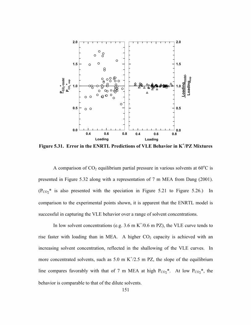
151
Loading0.4 0.6 0.8
Loa
ding
mod
el
Load
ing e
xp
0.0
0.5
1.0
1.5
2.0
Loading0.4 0.6 0.8
P CO
2* mod
el
P CO
2* exp
0.0
0.5
1.0
1.5
2.0
Figure 5.31. Error in the ENRTL Predictions of VLE Behavior in K+/PZ Mixtures
A comparison of CO2 equilibrium partial pressure in various solvents at 60oC is
presented in Figure 5.32 along with a representation of 7 m MEA from Dang (2001).
(PCO2* is also presented with the speciation in Figure 5.21 to Figure 5.26.) In
comparison to the experimental points shown, it is apparent that the ENRTL model is
successful in capturing the VLE behavior over a range of solvent concentrations.
In low solvent concentrations (e.g. 3.6 m K+/0.6 m PZ), the VLE curve tends to
rise faster with loading than in MEA. A higher CO2 capacity is achieved with an
increasing solvent concentration, reflected in the shallowing of the VLE curves. In
more concentrated solvents, such as 5.0 m K+/2.5 m PZ, the slope of the equilibrium
line compares favorably with that of 7 m MEA at high PCO2*. At low PCO2*, the
behavior is comparable to that of the dilute solvents.
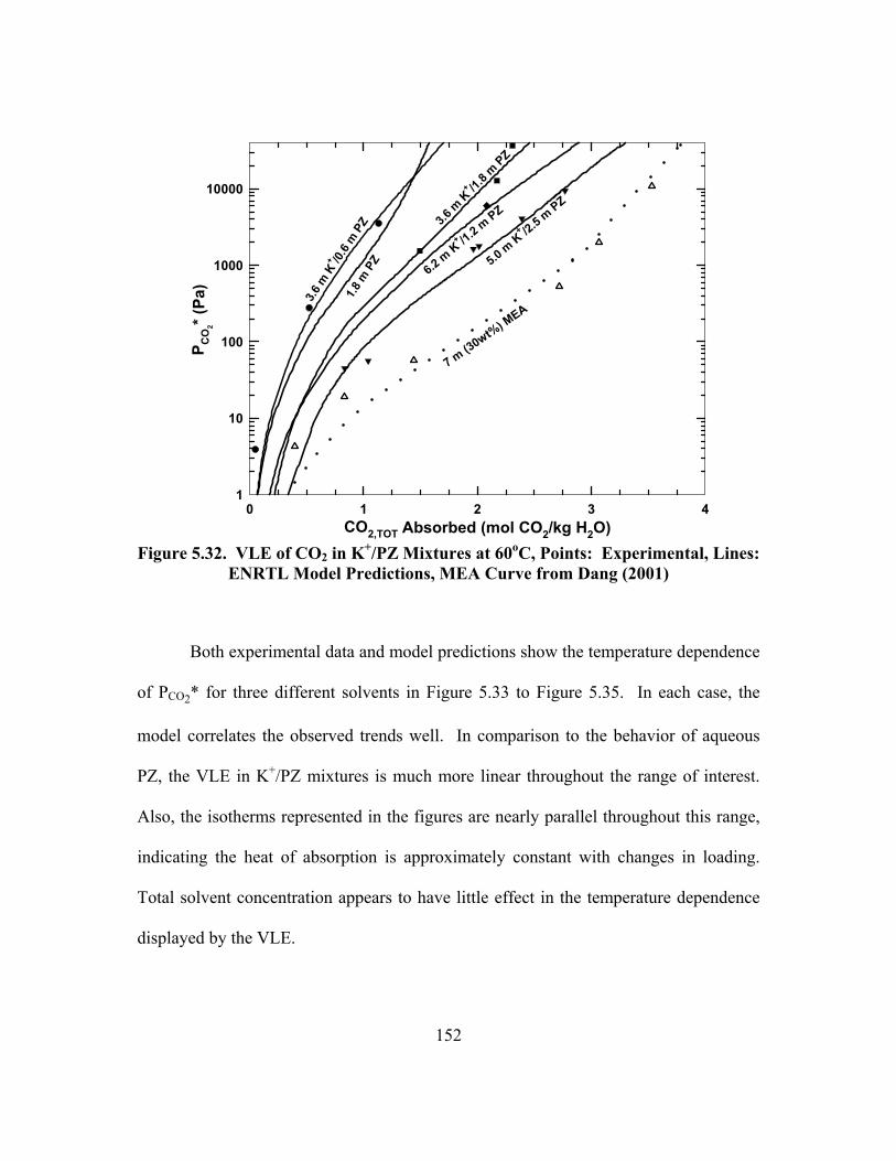
152
CO2,TOT Absorbed (mol CO2/kg H2O)0 1 2 3 4
P CO
2* (Pa
)
1
10
100
1000
10000
1.8 m
PZ
3.6 m
K+ /0.
6 m P
Z 3.6 m
K+ /1.
8 m PZ
5.0 m K
+ /2.5 m PZ
7 m (30wt%) M
EA
6.2 m K
+ /1.2 m PZ
Figure 5.32. VLE of CO2 in K+/PZ Mixtures at 60oC, Points: Experimental, Lines:
ENRTL Model Predictions, MEA Curve from Dang (2001)
Both experimental data and model predictions show the temperature dependence
of PCO2* for three different solvents in Figure 5.33 to Figure 5.35. In each case, the
model correlates the observed trends well. In comparison to the behavior of aqueous
PZ, the VLE in K+/PZ mixtures is much more linear throughout the range of interest.
Also, the isotherms represented in the figures are nearly parallel throughout this range,
indicating the heat of absorption is approximately constant with changes in loading.
Total solvent concentration appears to have little effect in the temperature dependence
displayed by the VLE.

153
Loading (mol CO2/(mol K+ + mol PZ))0.4 0.5 0.6 0.7 0.8 0.9
P CO
2* (Pa
)
10
100
1000
10000
40o C60o C80o C
100o C 110o C
Figure 5.33. Temperature Dependence of PCO2* in 3.6 m K+/0.6 m PZ
Loading (mol CO2/(mol K+ + mol PZ))0.3 0.4 0.5 0.6 0.7 0.8 0.9
P CO
2* (Pa
)
10
100
1000
10000
40o C60
o C80o C
100o C
110o C
Figure 5.34. Temperature Dependence of PCO2* in 3.6 m K+/1.8 m PZ
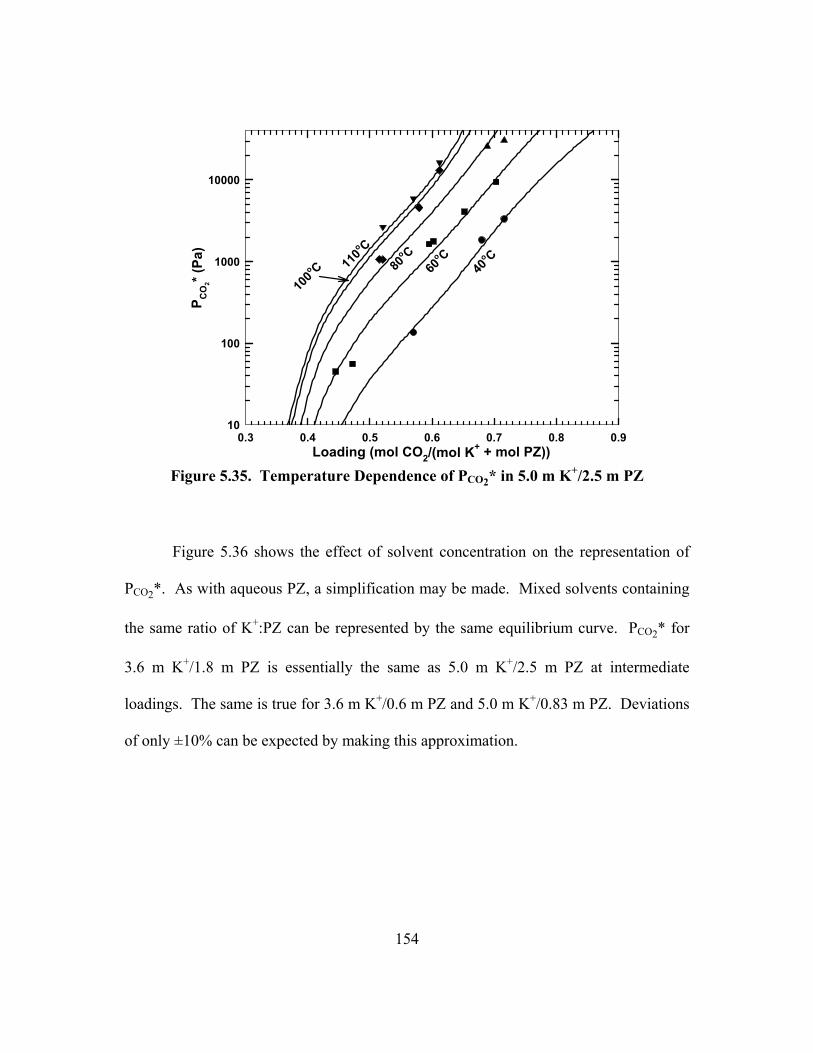
154
Loading (mol CO2/(mol K+ + mol PZ))0.3 0.4 0.5 0.6 0.7 0.8 0.9
P CO
2* (Pa
)
10
100
1000
10000
40o C
60o C
80o C
100o C 11
0o C
Figure 5.35. Temperature Dependence of PCO2* in 5.0 m K+/2.5 m PZ
Figure 5.36 shows the effect of solvent concentration on the representation of
PCO2*. As with aqueous PZ, a simplification may be made. Mixed solvents containing
the same ratio of K+:PZ can be represented by the same equilibrium curve. PCO2* for
3.6 m K+/1.8 m PZ is essentially the same as 5.0 m K+/2.5 m PZ at intermediate
loadings. The same is true for 3.6 m K+/0.6 m PZ and 5.0 m K+/0.83 m PZ. Deviations
of only ±10% can be expected by making this approximation.
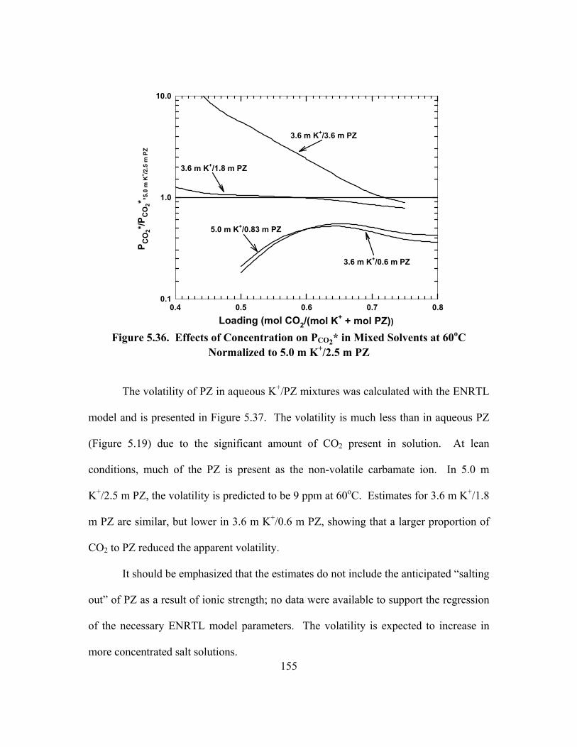
155
Loading (mol CO2/(mol K+ + mol PZ))0.4 0.5 0.6 0.7 0.8
P CO
2*/PC
O2*, 5.
0 m
K+ /2
.5 m
PZ
0.1
1.0
10.0
3.6 m K+/0.6 m PZ
5.0 m K+/0.83 m PZ
3.6 m K+/3.6 m PZ
3.6 m K+/1.8 m PZ
Figure 5.36. Effects of Concentration on PCO2* in Mixed Solvents at 60oC
Normalized to 5.0 m K+/2.5 m PZ
The volatility of PZ in aqueous K+/PZ mixtures was calculated with the ENRTL
model and is presented in Figure 5.37. The volatility is much less than in aqueous PZ
(Figure 5.19) due to the significant amount of CO2 present in solution. At lean
conditions, much of the PZ is present as the non-volatile carbamate ion. In 5.0 m
K+/2.5 m PZ, the volatility is predicted to be 9 ppm at 60oC. Estimates for 3.6 m K+/1.8
m PZ are similar, but lower in 3.6 m K+/0.6 m PZ, showing that a larger proportion of
CO2 to PZ reduced the apparent volatility.
It should be emphasized that the estimates do not include the anticipated �salting
out� of PZ as a result of ionic strength; no data were available to support the regression
of the necessary ENRTL model parameters. The volatility is expected to increase in
more concentrated salt solutions.
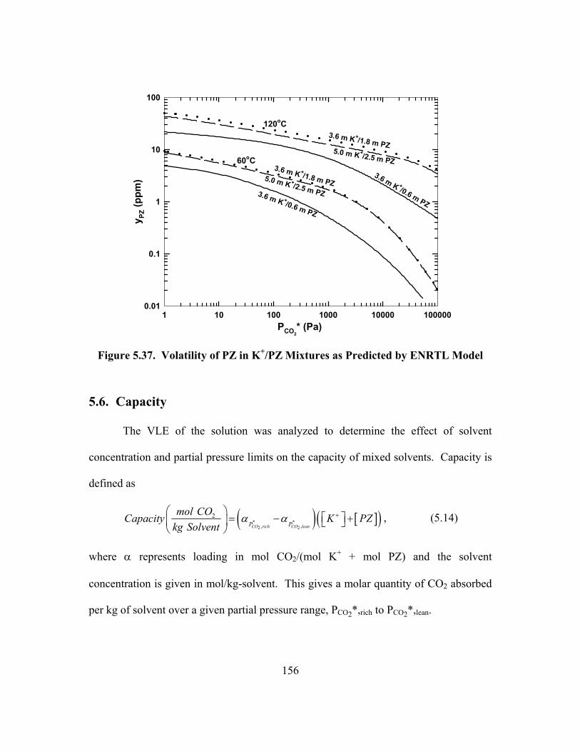
156
PCO2* (Pa)
1 10 100 1000 10000 100000
y PZ (p
pm)
0.01
0.1
1
10
100
3.6 m K +/1.8 m PZ3.6 m K +/0.6 m PZ
5.0 m K +/2.5 m PZ
3.6 m K+/1.8 m PZ
3.6 m K +/0.6 m PZ
5.0 m K+/2.5 m PZ60oC
120oC
Figure 5.37. Volatility of PZ in K+/PZ Mixtures as Predicted by ENRTL Model
5.6. Capacity
The VLE of the solution was analyzed to determine the effect of solvent
concentration and partial pressure limits on the capacity of mixed solvents. Capacity is
defined as
( ) [ ]( )* *, ,2 2
2 CO rich CO leanP P
mol COCapacity K PZkg Solvent
α α + = − +
, (5.14)
where α represents loading in mol CO2/(mol K+ + mol PZ) and the solvent
concentration is given in mol/kg-solvent. This gives a molar quantity of CO2 absorbed
per kg of solvent over a given partial pressure range, PCO2*,rich to PCO2*,lean.

157
In Figure 5.38, the effects of lean loading and concentration are demonstrated.
One observation is that the capacity, regardless of the partial pressure range, is a nearly
linear function of the total solution alkalinity. Another is that capacity increases with a
decrease in lean loading, which is expected as more of the VLE curve is used. In
comparison to 5 M MEA, the capacity of the K+/PZ solvent is less competitive as the
lean loading is decreased. This is a function of the shape of the VLE curves. From
Figure 5.32, it is shown that MEA has a much shallower VLE curve at low PCO2*,
increasing its effective capacity. Operating at PCO2*,lean = 100 Pa, a total alkalinity of 7
mol/kg is required to equal the capacity of 5 M MEA. At PCO2*,lean = 10 Pa, MEA has a
significant capacity advantage over even concentrated K+/PZ blends.
[K+] + 2[PZ] (mol/kg Solvent)3 4 5 6 7 8
Cap
acity
(mol
CO
2/kg
Solv
ent)
0.0
0.5
1.0
1.5
0.0 m K+/1.8 m PZ
3.6/0.6 3.6/1.85 M MEA 3.6/3.65.0/2.56.2/1.23.6/0.0
PCO2*,lean = 1,000 Pa
PCO2*, lean = 100 Pa
PCO2*, lean = 10 Pa
Figure 5.38. Capacity of K+/PZ Solvents at 60oC, PCO2*,rich = 3,000 Pa, Points:
Calculated from ENRTL Model, Lines: Straight Line Fit of Points
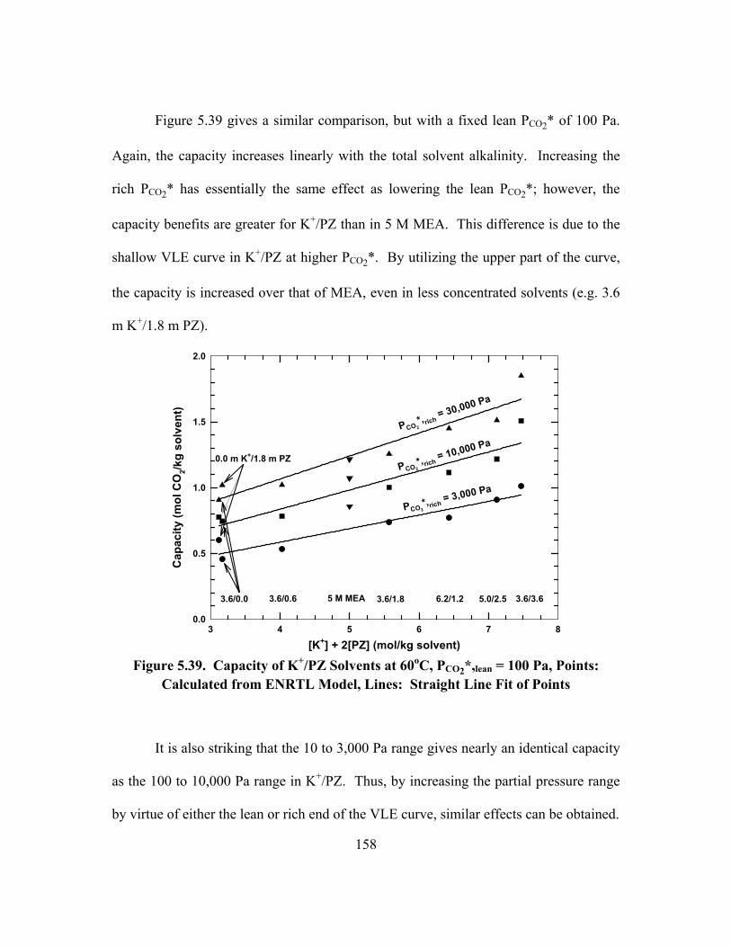
158
Figure 5.39 gives a similar comparison, but with a fixed lean PCO2* of 100 Pa.
Again, the capacity increases linearly with the total solvent alkalinity. Increasing the
rich PCO2* has essentially the same effect as lowering the lean PCO2*; however, the
capacity benefits are greater for K+/PZ than in 5 M MEA. This difference is due to the
shallow VLE curve in K+/PZ at higher PCO2*. By utilizing the upper part of the curve,
the capacity is increased over that of MEA, even in less concentrated solvents (e.g. 3.6
m K+/1.8 m PZ).
[K+] + 2[PZ] (mol/kg solvent)3 4 5 6 7 8
Cap
acity
(mol
CO
2/kg
solv
ent)
0.0
0.5
1.0
1.5
2.0
0.0 m K+/1.8 m PZ
3.6/0.6 3.6/1.85 M MEA 3.6/3.65.0/2.56.2/1.23.6/0.0
PCO2*, rich = 30,000 Pa
PCO2*,rich = 10,000 Pa
PCO2*,rich = 3,000 Pa
Figure 5.39. Capacity of K+/PZ Solvents at 60oC, PCO2*,lean = 100 Pa, Points:
Calculated from ENRTL Model, Lines: Straight Line Fit of Points
It is also striking that the 10 to 3,000 Pa range gives nearly an identical capacity
as the 100 to 10,000 Pa range in K+/PZ. Thus, by increasing the partial pressure range
by virtue of either the lean or rich end of the VLE curve, similar effects can be obtained.
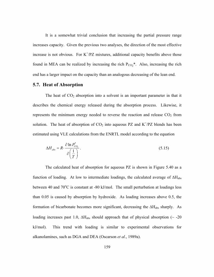
159
It is a somewhat trivial conclusion that increasing the partial pressure range
increases capacity. Given the previous two analyses, the direction of the most effective
increase is not obvious. For K+/PZ mixtures, additional capacity benefits above those
found in MEA can be realized by increasing the rich PCO2*. Also, increasing the rich
end has a larger impact on the capacity than an analogous decreasing of the lean end.
5.7. Heat of Absorption
The heat of CO2 absorption into a solvent is an important parameter in that it
describes the chemical energy released during the absorption process. Likewise, it
represents the minimum energy needed to reverse the reaction and release CO2 from
solution. The heat of absorption of CO2 into aqueous PZ and K+/PZ blends has been
estimated using VLE calculations from the ENRTL model according to the equation
2
*ln1
COabs
PH R
T
∂∆ = ⋅
∂
. (5.15)
The calculated heat of absorption for aqueous PZ is shown in Figure 5.40 as a
function of loading. At low to intermediate loadings, the calculated average of ∆Habs
between 40 and 70oC is constant at -80 kJ/mol. The small perturbation at loadings less
than 0.05 is caused by absorption by hydroxide. As loading increases above 0.5, the
formation of bicarbonate becomes more significant, decreasing the ∆Habs sharply. As
loading increases past 1.0, ∆Habs should approach that of physical absorption (~ -20
kJ/mol). This trend with loading is similar to experimental observations for
alkanolamines, such as DGA and DEA (Oscarson et al., 1989a).
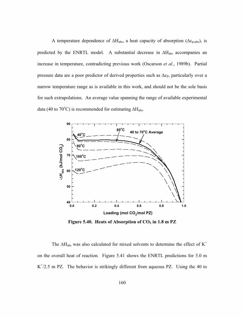
160
A temperature dependence of ∆Habs, a heat capacity of absorption (∆cp,abs), is
predicted by the ENRTL model. A substantial decrease in ∆Habs accompanies an
increase in temperature, contradicting previous work (Oscarson et al., 1989b). Partial
pressure data are a poor predictor of derived properties such as ∆cP, particularly over a
narrow temperature range as is available in this work, and should not be the sole basis
for such extrapolations. An average value spanning the range of available experimental
data (40 to 70oC) is recommended for estimating ∆Habs.
Loading (mol CO2/mol PZ)
0.0 0.2 0.4 0.6 0.8 1.0
- ∆H
abs (
kJ/m
ol C
O2)
40
50
60
70
80
90
40oC60oC
80oC
100oC
120oC
40 to 70oC Average
Figure 5.40. Heats of Absorption of CO2 in 1.8 m PZ
The ∆Habs was also calculated for mixed solvents to determine the effect of K+
on the overall heat of reaction. Figure 5.41 shows the ENRTL predictions for 5.0 m
K+/2.5 m PZ. The behavior is strikingly different from aqueous PZ. Using the 40 to
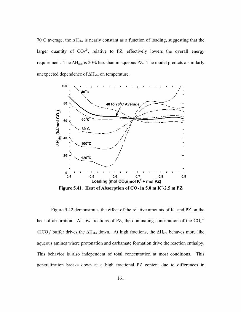
161
70oC average, the ∆Habs is nearly constant as a function of loading, suggesting that the
larger quantity of CO32-, relative to PZ, effectively lowers the overall energy
requirement. The ∆Habs is 20% less than in aqueous PZ. The model predicts a similarly
unexpected dependence of ∆Habs on temperature.
Loading (mol CO2/(mol K+ + mol PZ)0.4 0.5 0.6 0.7 0.8 0.9
- ∆H
abs (
kJ/m
ol C
O2)
0
20
40
60
80
100
40oC
60oC
80oC
100oC
120oC
40 to 70oC Average
Figure 5.41. Heat of Absorption of CO2 in 5.0 m K+/2.5 m PZ
Figure 5.42 demonstrates the effect of the relative amounts of K+ and PZ on the
heat of absorption. At low fractions of PZ, the dominating contribution of the CO32-
/HCO3- buffer drives the ∆Habs down. At high fractions, the ∆Habs behaves more like
aqueous amines where protonation and carbamate formation drive the reaction enthalpy.
This behavior is also independent of total concentration at most conditions. This
generalization breaks down at a high fractional PZ content due to differences in
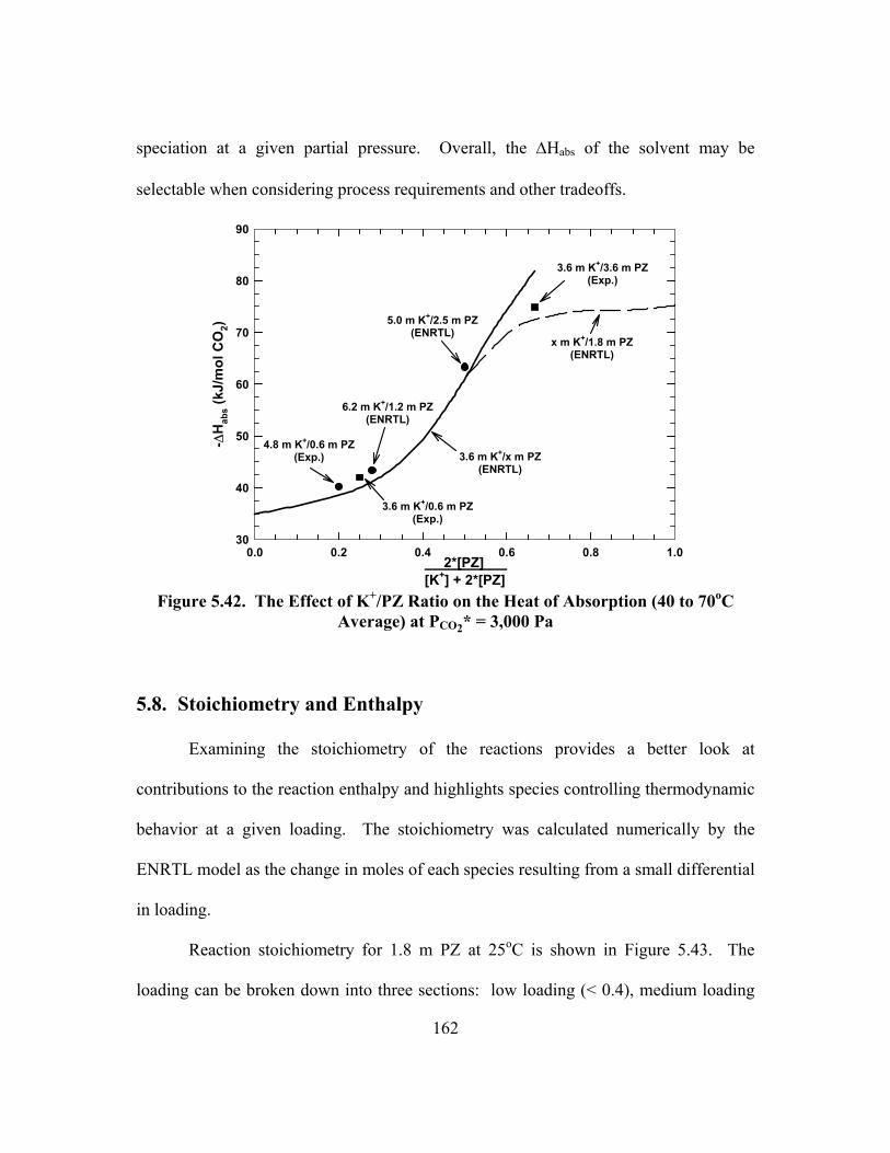
162
speciation at a given partial pressure. Overall, the ∆Habs of the solvent may be
selectable when considering process requirements and other tradeoffs.
2*[PZ] [K+] + 2*[PZ]
0.0 0.2 0.4 0.6 0.8 1.0
- ∆H
abs (
kJ/m
ol C
O2)
30
40
50
60
70
80
90
3.6 m K+/x m PZ(ENRTL)
x m K+/1.8 m PZ(ENRTL)
5.0 m K+/2.5 m PZ(ENRTL)
6.2 m K+/1.2 m PZ(ENRTL)
3.6 m K+/3.6 m PZ(Exp.)
3.6 m K+/0.6 m PZ(Exp.)
4.8 m K+/0.6 m PZ(Exp.)
Figure 5.42. The Effect of K+/PZ Ratio on the Heat of Absorption (40 to 70oC
Average) at PCO2* = 3,000 Pa
5.8. Stoichiometry and Enthalpy
Examining the stoichiometry of the reactions provides a better look at
contributions to the reaction enthalpy and highlights species controlling thermodynamic
behavior at a given loading. The stoichiometry was calculated numerically by the
ENRTL model as the change in moles of each species resulting from a small differential
in loading.
Reaction stoichiometry for 1.8 m PZ at 25oC is shown in Figure 5.43. The
loading can be broken down into three sections: low loading (< 0.4), medium loading
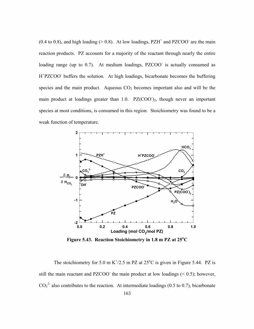
163
(0.4 to 0.8), and high loading (> 0.8). At low loadings, PZH+ and PZCOO- are the main
reaction products. PZ accounts for a majority of the reactant through nearly the entire
loading range (up to 0.7). At medium loadings, PZCOO- is actually consumed as
H+PZCOO- buffers the solution. At high loadings, bicarbonate becomes the buffering
species and the main product. Aqueous CO2 becomes important also and will be the
main product at loadings greater than 1.0. PZ(COO-)2, though never an important
species at most conditions, is consumed in this region. Stoichiometry was found to be a
weak function of temperature.
Loading (mol CO2/mol PZ)0.0 0.2 0.4 0.6 0.8 1.0
δ ni δ nCO2
-2
-1
0
1
2
CO32-
H+PZCOO-PZH+
PZCOO-
PZ
PZ(COO-)2
HCO3-
OH-
CO2
H2O
Figure 5.43. Reaction Stoichiometry in 1.8 m PZ at 25oC
The stoichiometry for 5.0 m K+/2.5 m PZ at 25oC is given in Figure 5.44. PZ is
still the main reactant and PZCOO- the main product at low loadings (< 0.5); however,
CO32- also contributes to the reaction. At intermediate loadings (0.5 to 0.7), bicarbonate
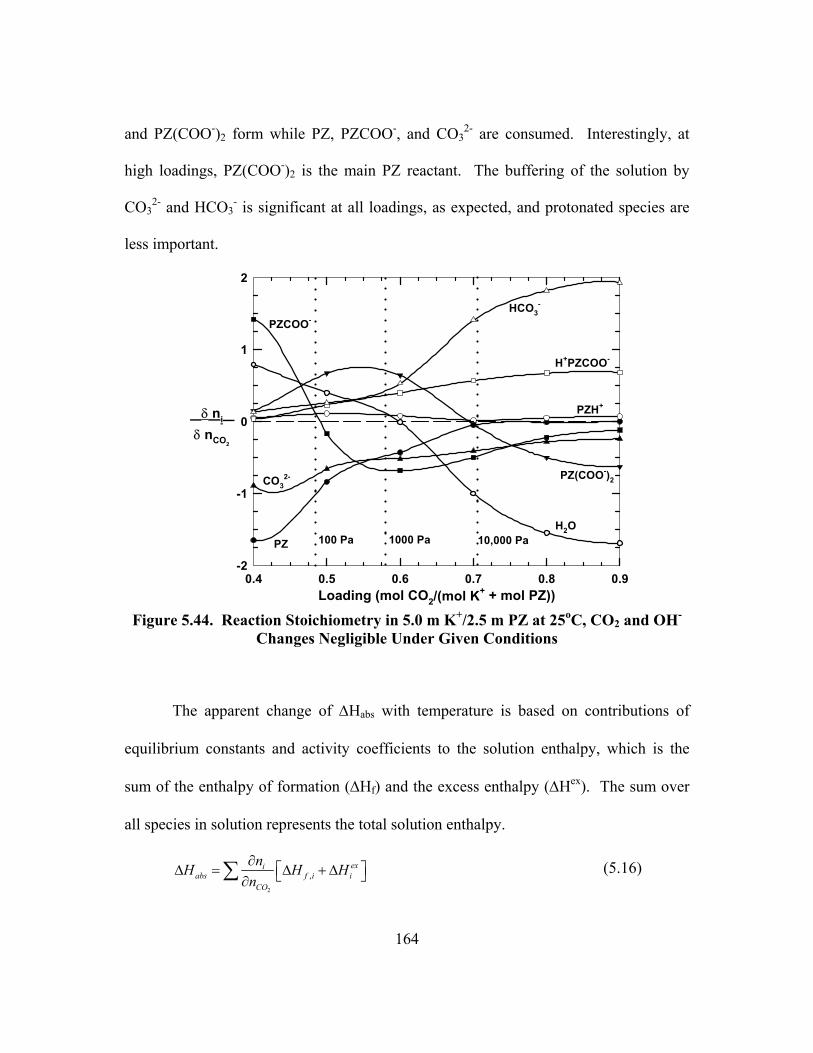
164
and PZ(COO-)2 form while PZ, PZCOO-, and CO32- are consumed. Interestingly, at
high loadings, PZ(COO-)2 is the main PZ reactant. The buffering of the solution by
CO32- and HCO3
- is significant at all loadings, as expected, and protonated species are
less important.
Loading (mol CO2/(mol K+ + mol PZ))0.4 0.5 0.6 0.7 0.8 0.9
δ ni δ nCO2
-2
-1
0
1
2
CO32-
H+PZCOO-
PZH+
PZCOO-
PZ
PZ(COO-)2
HCO3-
H2O10,000 Pa1000 Pa100 Pa
Figure 5.44. Reaction Stoichiometry in 5.0 m K+/2.5 m PZ at 25oC, CO2 and OH-
Changes Negligible Under Given Conditions
The apparent change of ∆Habs with temperature is based on contributions of
equilibrium constants and activity coefficients to the solution enthalpy, which is the
sum of the enthalpy of formation (∆Hf) and the excess enthalpy (∆Hex). The sum over
all species in solution represents the total solution enthalpy.
2
,exi
abs f i iCO
nH H Hn∂ ∆ = ∆ + ∆ ∂∑ (5.16)
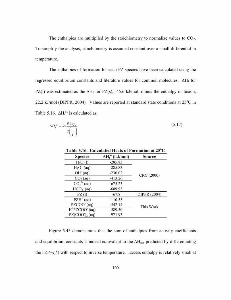
165
The enthalpies are multiplied by the stoichiometry to normalize values to CO2.
To simplify the analysis, stoichiometry is assumed constant over a small differential in
temperature.
The enthalpies of formation for each PZ species have been calculated using the
regressed equilibrium constants and literature values for common molecules. ∆Hf for
PZ(l) was estimated as the ∆Hf for PZ(s), -45.6 kJ/mol, minus the enthalpy of fusion,
22.2 kJ/mol (DIPPR, 2004). Values are reported at standard state conditions at 25oC in
Table 5.16. ∆Hiex is calculated as
ln1
ex iiH R
T
γ∂∆ = ⋅
∂
. (5.17)
Table 5.16. Calculated Heats of Formation at 25oC
Species ∆Hfo (kJ/mol) Source
H2O (l) -285.83 H3O+ (aq) -285.83 OH- (aq) -230.02 CO2 (aq) -413.26
CO32- (aq) -675.23
HCO3- (aq) -689.93
CRC (2000)
PZ (l) -67.8 DIPPR (2004) PZH+ (aq) -110.55
PZCOO- (aq) -542.14 H+PZCOO- (aq) -589.50 PZ(COO-)2 (aq) -971.93
This Work
Figure 5.45 demonstrates that the sum of enthalpies from activity coefficients
and equilibrium constants is indeed equivalent to the ∆Habs predicted by differentiating
the ln(PCO2*) with respect to inverse temperature. Excess enthalpy is relatively small at
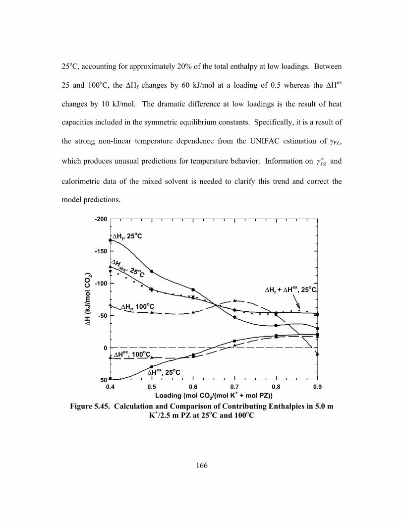
166
25oC, accounting for approximately 20% of the total enthalpy at low loadings. Between
25 and 100oC, the ∆Hf changes by 60 kJ/mol at a loading of 0.5 whereas the ∆Hex
changes by 10 kJ/mol. The dramatic difference at low loadings is the result of heat
capacities included in the symmetric equilibrium constants. Specifically, it is a result of
the strong non-linear temperature dependence from the UNIFAC estimation of γPZ,
which produces unusual predictions for temperature behavior. Information on PZγ ∞ and
calorimetric data of the mixed solvent is needed to clarify this trend and correct the
model predictions.
Loading (mol CO2/(mol K+ + mol PZ))0.4 0.5 0.6 0.7 0.8 0.9
∆H
(kJ/
mol
CO
2)
-200
-150
-100
-50
0
50
∆Hf + ∆Hex, 25oC
∆Habs , 25 oC
∆Hex, 100oC
∆Hex, 25oC
∆Hf, 100oC
∆Hf, 25oC
Figure 5.45. Calculation and Comparison of Contributing Enthalpies in 5.0 m
K+/2.5 m PZ at 25oC and 100oC
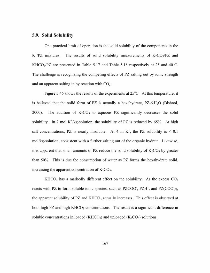
167
5.9. Solid Solubility
One practical limit of operation is the solid solubility of the components in the
K+/PZ mixtures. The results of solid solubility measurements of K2CO3/PZ and
KHCO3/PZ are presented in Table 5.17 and Table 5.18 respectively at 25 and 40oC.
The challenge is recognizing the competing effects of PZ salting out by ionic strength
and an apparent salting in by reaction with CO2.
Figure 5.46 shows the results of the experiments at 25oC. At this temperature, it
is believed that the solid form of PZ is actually a hexahydrate, PZ-6·H2O (Bishnoi,
2000). The addition of K2CO3 to aqueous PZ significantly decreases the solid
solubility. In 2 mol K+/kg-solution, the solubility of PZ is reduced by 65%. At high
salt concentrations, PZ is nearly insoluble. At 4 m K+, the PZ solubility is < 0.1
mol/kg-solution, consistent with a further salting out of the organic hydrate. Likewise,
it is apparent that small amounts of PZ reduce the solid solubility of K2CO3 by greater
than 50%. This is due the consumption of water as PZ forms the hexahydrate solid,
increasing the apparent concentration of K2CO3.
KHCO3 has a markedly different effect on the solubility. As the excess CO2
reacts with PZ to form soluble ionic species, such as PZCOO-, PZH+, and PZ(COO-)2,
the apparent solubility of PZ and KHCO3 actually increases. This effect is observed at
both high PZ and high KHCO3 concentrations. The result is a significant difference in
soluble concentrations in loaded (KHCO3) and unloaded (K2CO3) solutions.
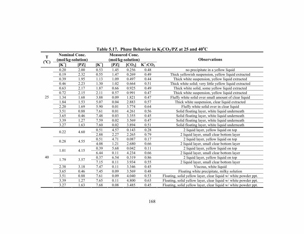
168
Table 5.17. Phase Behavior in K2CO3/PZ at 25 and 40oC Nominal Conc.
(mol/kg-solution) Measured Conc. (mol/kg-solution) T
(oC) [K+] [PZ] [K+] [PZ] [CO2] K+:CO2
Observations
0.20 2.00 0.53 1.45 0.256 0.48 no precipitate in a yellow liquid 0.19 2.32 0.55 1.47 0.269 0.49 Thick yellowish suspension, yellow liquid extracted 0.39 1.95 1.13 1.09 0.497 0.44 Thick white suspension, yellow liquid extracted 0.46 2.23 1.30 1.02 0.664 0.51 Thick white solid; very little yellow liquid extracted 0.63 2.17 1.87 0.66 0.925 0.49 Thick white solid, some yellow liquid extracted 0.72 2.15 2.11 0.57 0.991 0.47 Thick white suspension, yellow liquid extracted 1.34 1.68 3.88 0.09 1.821 0.47 Fluffy white solid over small amount of clear liquid 1.84 1.53 5.07 0.04 2.883 0.57 Thick white suspension, clear liquid extracted 2.20 1.69 5.90 0.01 3.774 0.64 Fluffy white solid over in clear liquid 3.51 0.88 7.61 0.01 4.261 0.56 Solid floating layer, white liquid underneath 3.65 0.46 7.48 0.03 3.355 0.45 Solid floating layer, white liquid underneath 3.39 1.27 7.59 0.02 3.569 0.47 Solid floating layer, white liquid underneath
25
3.27 1.63 7.60 0.02 3.894 0.51 Solid floating layer, white liquid underneath 0.51 4.57 0.143 0.28 2 liquid layer, yellow liquid on top 0.22 4.60 2.88 2.27 2.265 0.79 2 liquid layer, small clear bottom layer 0.51 4.71 0.087 0.17 2 liquid layer, yellow liquid on top 0.28 4.55 4.08 1.21 2.680 0.66 2 liquid layer, small clear bottom layer 0.39 5.68 0.042 0.11 2 liquid layer, yellow liquid on top 1.01 4.15 6.44 0.11 4.234 0.66 2 liquid layer, small clear bottom layer 0.37 6.54 0.319 0.86 2 liquid layer, yellow liquid on top 1.79 3.57 7.15 0.11 3.934 0.55 2 liquid layer, small clear bottom layer
2.38 3.18 7.47 0.11 3.346 0.45 Viscous, white liquid 3.65 0.46 7.45 0.09 3.569 0.48 Floating white precipitate, milky solution 3.51 0.88 7.61 0.09 4.040 0.53 Floating, solid yellow layer, clear liquid w/ white powder ppt. 3.39 1.27 7.65 0.11 4.800 0.63 Floating, solid yellow layer, clear liquid w/ white powder ppt.
40
3.27 1.63 7.68 0.08 3.485 0.45 Floating, solid yellow layer, clear liquid w/ white powder ppt.

169
Table 5.18. Phase Behavior in KHCO3/PZ at 25 and 40oC Nominal Conc.
(mol/kg-solution) Measured Conc. (mol/kg-solution) T
(oC) [K+] [PZ] [K+] [PZ] [CO2] K+:CO2
Observations
0.34 3.38 0.49 1.92 0.717 1.46 Thick white solution, little yellow liquid extracted 0.65 3.29 1.27 1.88 2.029 1.60 White slush, yellow liquid extracted 1.23 3.07 1.82 2.00 1.729 0.95 White slush, yellow liquid extracted 2.19 2.71 2.45 2.27 2.912 1.19 Yellowish slush, thick yellow liquid extracted 2.39 2.66 2.53 2.35 2.270 0.90 Clear liquid on top of thick suspension, yellow liquid extracted 2.71 2.17 2.51 2.03 2.326 0.93 Clear liquid with white granular ppt. 3.65 0.30 2.97 0.32 2.546 0.86 Clear liquid with white granular ppt. 3.56 0.59 2.94 0.62 2.682 0.91 Clear liquid with white granular ppt. 3.39 1.13 3.20 1.09 3.451 1.08 Clear liquid with white granular ppt. 3.23 1.62 3.07 1.43 2.992 0.97 Clear liquid with white granular ppt. 3.16 1.84 2.87 1.60 2.520 0.88 Clear liquid with white granular ppt. 2.95 2.46 2.54 2.15 2.458 0.97 Clear liquid with white granular ppt. 2.83 2.83 2.47 2.58 2.244 0.91 Clear liquid with white granular ppt.
25
3.89 1.46 3.24 1.28 3.309 1.02 Yellow liquid with white granular ppt. 0.21 6.59 0.57 6.54 0.208 0.36 Opaque yellow solution with a white ppt. 0.51 5.10 1.03 4.86 0.218 0.21 Yellow liquid with ppt. 0.97 4.85 1.67 4.37 0.834 0.50 Yellow liquid with ppt. 1.92 3.83 1.74 3.64 1.668 0.96 White viscous liquid 3.89 1.46 3.33 1.21 3.265 0.98 Yellow liquid with white powder ppt. 3.21 3.21 1.97 2.75 2.032 1.03 Thick white suspension, filtered to a yellow liquid 4.27 1.71 3.54 1.16 3.667 1.04 Yellow liquid over a white ppt. 4.11 2.06 3.00 1.55 2.843 0.95 Yellow liquid over a white ppt. 3.72 2.97 2.24 3.15 2.225 0.99 Yellow liquid over a white ppt. 4.72 1.57 3.23 1.28 3.526 1.09 Yellow liquid over a white ppt. 5.96 0.37 3.15 0.62 2.395 0.76 Clear solution white ppt. 5.77 0.72 3.46 1.08 2.297 0.66 Clear solution white ppt.
40
5.60 1.05 3.50 1.14 2.331 0.67 Clear solution white ppt.
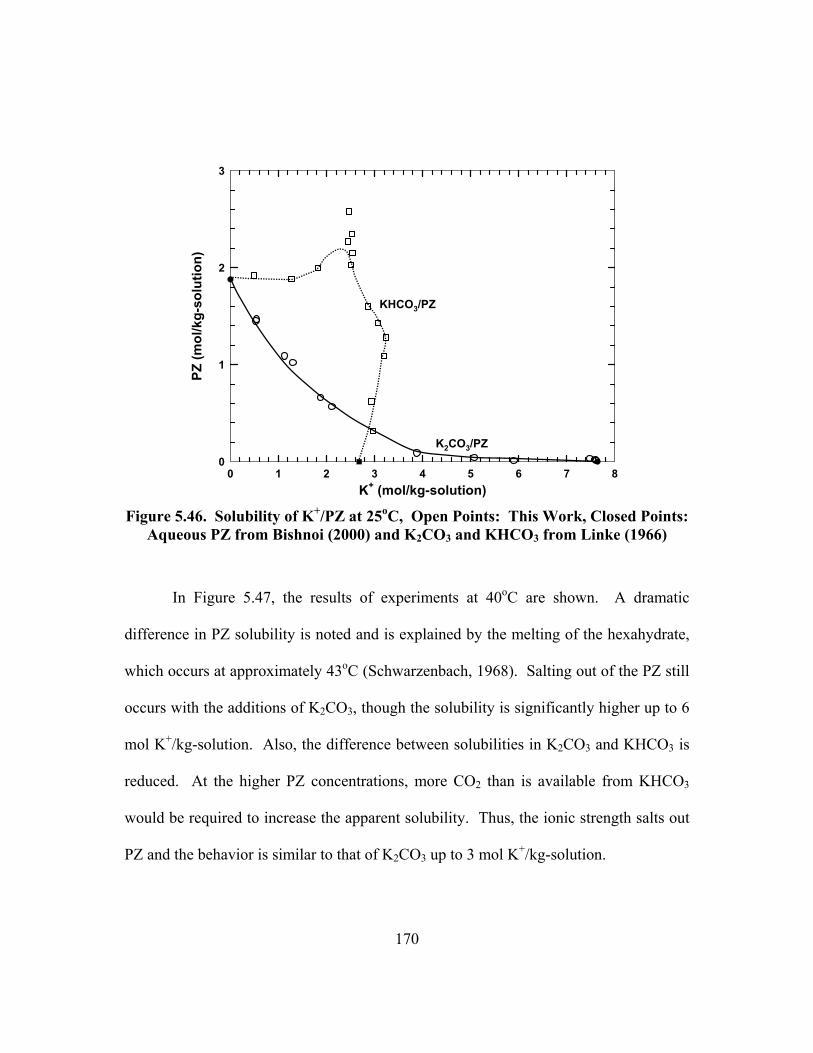
170
K+ (mol/kg-solution)0 1 2 3 4 5 6 7 8
PZ (m
ol/k
g-so
lutio
n)
0
1
2
3
K2CO3/PZ
KHCO3/PZ
Figure 5.46. Solubility of K+/PZ at 25oC, Open Points: This Work, Closed Points:
Aqueous PZ from Bishnoi (2000) and K2CO3 and KHCO3 from Linke (1966)
In Figure 5.47, the results of experiments at 40oC are shown. A dramatic
difference in PZ solubility is noted and is explained by the melting of the hexahydrate,
which occurs at approximately 43oC (Schwarzenbach, 1968). Salting out of the PZ still
occurs with the additions of K2CO3, though the solubility is significantly higher up to 6
mol K+/kg-solution. Also, the difference between solubilities in K2CO3 and KHCO3 is
reduced. At the higher PZ concentrations, more CO2 than is available from KHCO3
would be required to increase the apparent solubility. Thus, the ionic strength salts out
PZ and the behavior is similar to that of K2CO3 up to 3 mol K+/kg-solution.
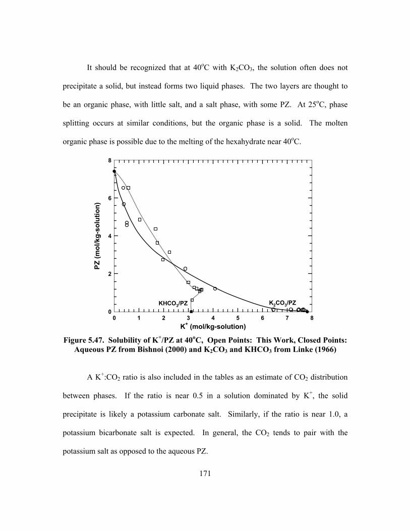
171
It should be recognized that at 40oC with K2CO3, the solution often does not
precipitate a solid, but instead forms two liquid phases. The two layers are thought to
be an organic phase, with little salt, and a salt phase, with some PZ. At 25oC, phase
splitting occurs at similar conditions, but the organic phase is a solid. The molten
organic phase is possible due to the melting of the hexahydrate near 40oC.
K+ (mol/kg-solution)0 1 2 3 4 5 6 7 8
PZ (m
ol/k
g-so
lutio
n)
0
2
4
6
8
K+ (mol/kg-solution)0 1 2 3 4 5 6 7 8
PZ (m
ol/k
g-so
lutio
n)
0
2
4
6
8
K2CO3/PZKHCO3/PZ
Figure 5.47. Solubility of K+/PZ at 40oC, Open Points: This Work, Closed Points:
Aqueous PZ from Bishnoi (2000) and K2CO3 and KHCO3 from Linke (1966)
A K+:CO2 ratio is also included in the tables as an estimate of CO2 distribution
between phases. If the ratio is near 0.5 in a solution dominated by K+, the solid
precipitate is likely a potassium carbonate salt. Similarly, if the ratio is near 1.0, a
potassium bicarbonate salt is expected. In general, the CO2 tends to pair with the
potassium salt as opposed to the aqueous PZ.
172
5.10. Conclusions
The ENRTL model adequately predicts the activity of water and PCO2* in
aqueous K2CO3 and KHCO3 solutions at various temperatures. The fit was achieved
using four τ parameters each with a small, linear temperature dependence. Future
inclusion of ion pair-ion pair interactions may improve inaccuracies at high salt
concentrations.
The ENRTL was fit to the UNIFAC predictions for γPZ. The model shows a
strong, non-linear dependence of γPZ on temperature and PZ concentration. Behavior at
infinite dilution in water gives a heat of solution that compares favorably with literature
values.
Relevant equilibrium constants for the reaction of CO2 with PZ have been
regressed as well as for the protonation of PZCOO-. The heats of reaction for the
formation of PZCOO- and PZ(COO-)2 are similar, 18.3 and 16.5 kJ/mol, as would be
expected by an analysis of structure. Likewise, the heat of reaction for the protonation
of PZCOO- is comparable to the heat of PZ protonation, at a value of -47.4 kJ/mol.
The fitted ENRTL model is able to represent aqueous PZ and K+/PZ speciation to
within an absolute error of 5%. VLE behavior is fairly well represented, deviating by
an apparent 25%. Most of the error, however, has been identified as in the solution
loading. A 10% error in loading can result in a 30% �error� in PCO2*. VLE behavior
suggests the solvent capacity increases as a linear function of solvent equivalents.
173
The speciation of PZ shows significant differences between aqueous PZ and
K+/PZ mixtures. In aqueous PZ, the carbamate species are never more than 20% of the
total PZ concentration. In contrast, each can account for as much as 50% with the
addition of K+. Protonation represents a significant amount of product from the
addition of CO2 to aqueous PZ. A high K+ concentration increases the prevalence of the
CO32-/HCO3
- buffer and delays protonation of the amine to high loadings. Thus,
carbamation of amines will increase in the presence of K+ to an extent related to the
carbamate stability. This effect is countered by the reduction of protonation afforded by
the strong buffer. The overall effect is an increase in reactive PZ concentration.
Model predictions show that the maximum reactive PZ concentration (PZ +
PZCOO-) occurs when the PZ concentration is maximized and K+ is added in a 2:1 ratio
of K+:PZ. The maximum concentration will be defined by the solid solubility limit
under any given condition.
VLE curves are depressed as total solution concentration increases, indicating
improved CO2 capacity in concentrated solvents. The addition of potassium improves
the VLE behavior of aqueous PZ.
The ∆Habs, at 40 to 70oC, is calculated to be -80 kJ/mol for aqueous PZ and -65
kJ/mol for K+/PZ mixtures, a reduction of 20%. Stoichiometry shows that the lower
enthalpy is obtained due to significant contribution of CO32- and the reduction in
protonation in mixed solvent reactions. Additionally, the ∆Habs may be �tuned� simply
by variation of the K+ to PZ ratio.
174
∆Habs is predicted to be a strong function of temperature and is a result of the
heat capacity predicted by UNIFAC for PZγ ∞ The model is therefore limited in
extrapolating second-order temperature effects, such as enthalpies, over broad ranges
and should be used with care to predict heats of CO2 absorption at extreme temperature.
Gathering experimental data for γPZ and ∆cP for the solution at various loadings should
be considered to correct this shortcoming.
175
Equation Chapter 6 Section 1
Chapter 6: Rate and Kinetics of Potassium Carbonate,
Piperazine and Carbon Dioxide Mixtures
This chapter presents experimental data and modeling results on CO2 absorption
into K+/PZ mixtures. The absorption rate of CO2 was measured in a wetted-wall
column in 0.45 to 3.6 m piperazine (PZ) and 0.0 to 3.1 m potassium carbonate (K2CO3)
at 25 to 110oC. A rigorous kinetic model was used to interpret diffusivities and rate
constants. The kinetics of important reactions were interpreted with the termolecular
mechanism. The rate constants were found to follow correlations provided by base
catalysis theory. The effect of neutral salts on the absorption rate in aqueous PZ was
also measured and accounted for within the rigorous model. Approximations were
developed to represent the absorption rate from the range of pseudo-first order to
instantaneous behavior. Limitations to the approximations and to the performance of
K+/PZ mixtures as applied at industrial conditions are discussed.
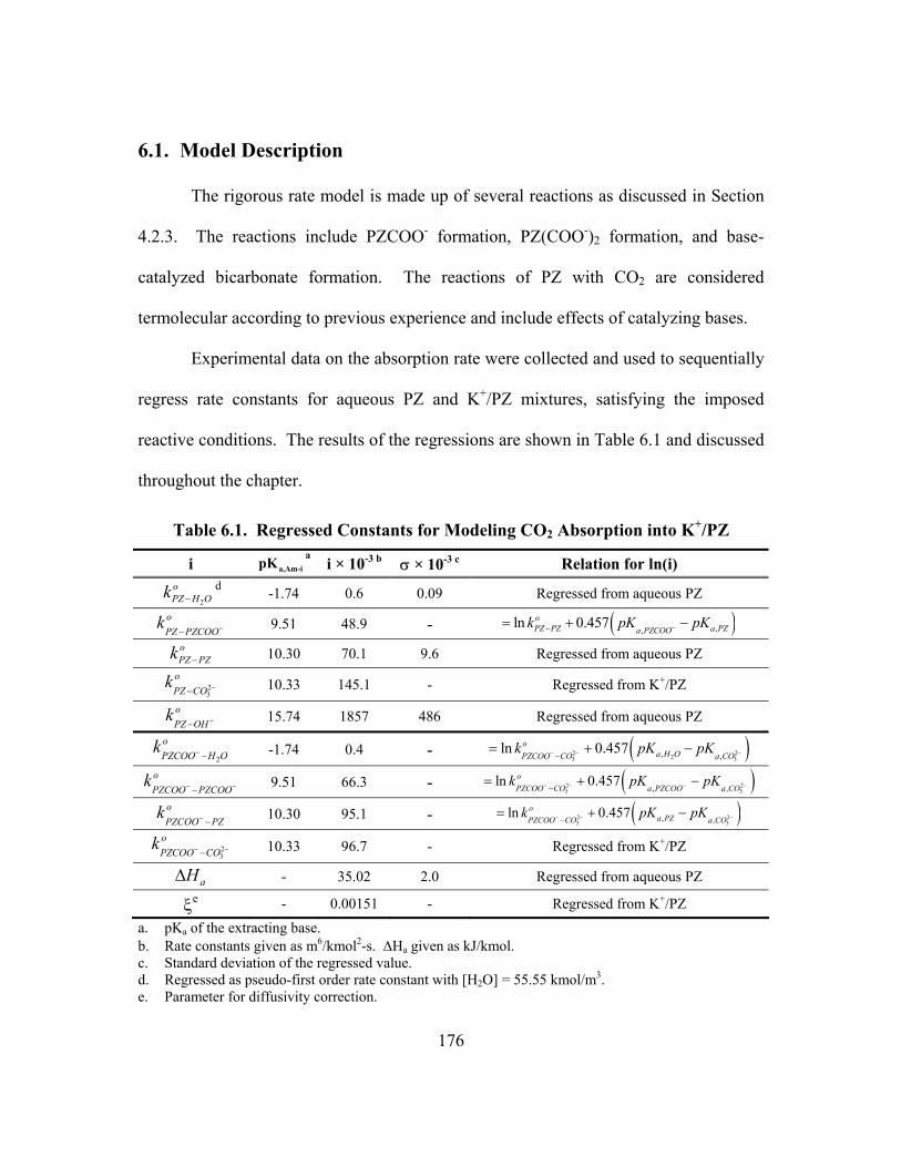
176
6.1. Model Description
The rigorous rate model is made up of several reactions as discussed in Section
4.2.3. The reactions include PZCOO- formation, PZ(COO-)2 formation, and base-
catalyzed bicarbonate formation. The reactions of PZ with CO2 are considered
termolecular according to previous experience and include effects of catalyzing bases.
Experimental data on the absorption rate were collected and used to sequentially
regress rate constants for aqueous PZ and K+/PZ mixtures, satisfying the imposed
reactive conditions. The results of the regressions are shown in Table 6.1 and discussed
throughout the chapter.
Table 6.1. Regressed Constants for Modeling CO2 Absorption into K+/PZ
i a,Am-ipKa
i × 10-3 b σ × 10-3 c Relation for ln(i)
2
oPZ H Ok −
d -1.74 0.6 0.09 Regressed from aqueous PZ oPZ PZCOO
k −− 9.51 48.9 - ( ),,
ln 0.457oPZ PZ a PZa PZCOO
k pK pK−−= + −
oPZ PZk − 10.30 70.1 9.6 Regressed from aqueous PZ
23
oPZ CO
k −− 10.33 145.1 - Regressed from K+/PZ
oPZ OH
k −− 15.74 1857 486 Regressed from aqueous PZ
2
oPZCOO H O
k − − -1.74 0.4 - ( )2 223 3
, ,ln 0.457o
a H OPZCOO CO a COk pK pK− − −−
= + −
oPZCOO PZCOO
k − −− 9.51 66.3 - ( )2 2
3 3, ,ln 0.457o
PZCOO CO a PZCOO a COk pK pK− − − −−
= + −
oPZCOO PZ
k − − 10.30 95.1 - ( )2 2
3 3, ,
ln 0.457oa PZPZCOO CO a CO
k pK pK− − −−= + −
23
oPZCOO CO
k − −− 10.33 96.7 - Regressed from K+/PZ
aH∆
- 35.02 2.0 Regressed from aqueous PZ
ξe - 0.00151 - Regressed from K+/PZ a. pKa of the extracting base. b. Rate constants given as m6/kmol2-s. ∆Ha given as kJ/kmol. c. Standard deviation of the regressed value. d. Regressed as pseudo-first order rate constant with [H2O] = 55.55 kmol/m3. e. Parameter for diffusivity correction.
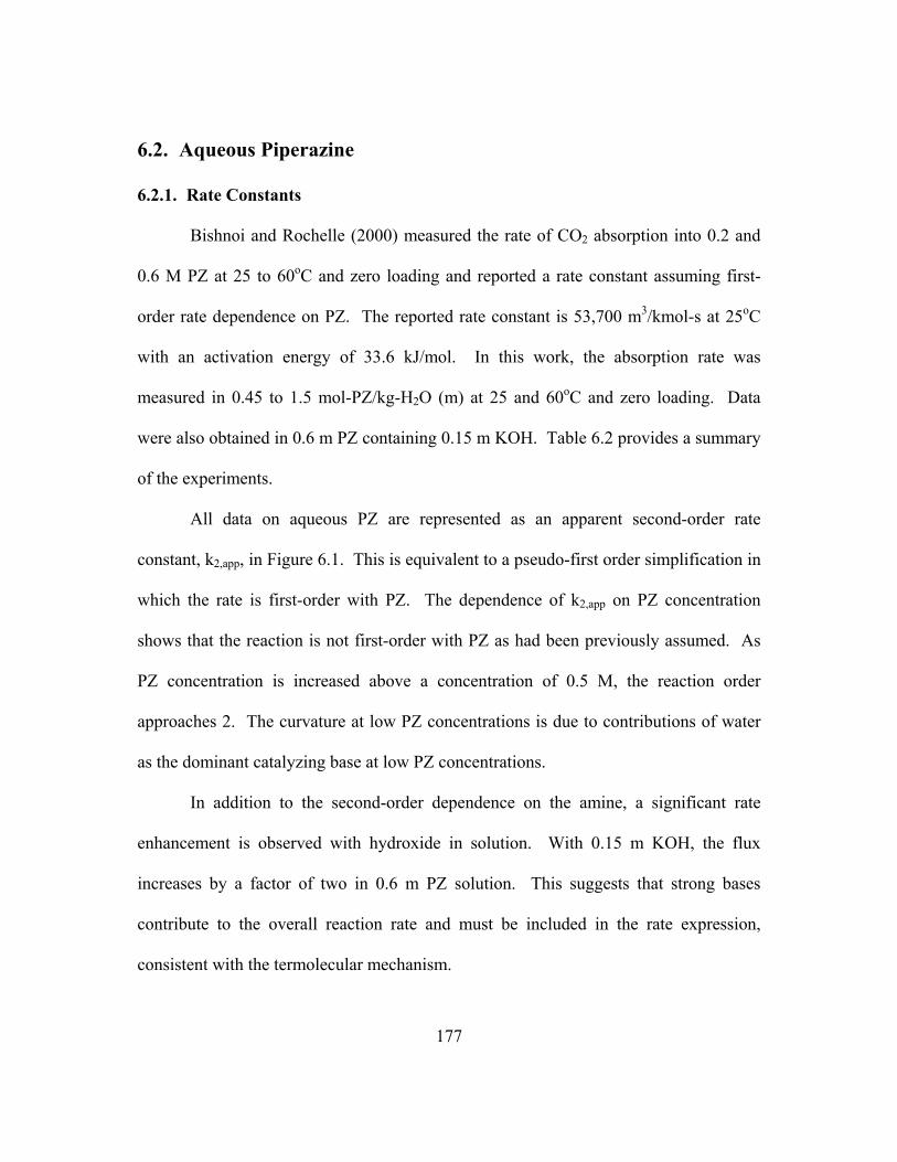
177
6.2. Aqueous Piperazine
6.2.1. Rate Constants
Bishnoi and Rochelle (2000) measured the rate of CO2 absorption into 0.2 and
0.6 M PZ at 25 to 60oC and zero loading and reported a rate constant assuming first-
order rate dependence on PZ. The reported rate constant is 53,700 m3/kmol-s at 25oC
with an activation energy of 33.6 kJ/mol. In this work, the absorption rate was
measured in 0.45 to 1.5 mol-PZ/kg-H2O (m) at 25 and 60oC and zero loading. Data
were also obtained in 0.6 m PZ containing 0.15 m KOH. Table 6.2 provides a summary
of the experiments.
All data on aqueous PZ are represented as an apparent second-order rate
constant, k2,app, in Figure 6.1. This is equivalent to a pseudo-first order simplification in
which the rate is first-order with PZ. The dependence of k2,app on PZ concentration
shows that the reaction is not first-order with PZ as had been previously assumed. As
PZ concentration is increased above a concentration of 0.5 M, the reaction order
approaches 2. The curvature at low PZ concentrations is due to contributions of water
as the dominant catalyzing base at low PZ concentrations.
In addition to the second-order dependence on the amine, a significant rate
enhancement is observed with hydroxide in solution. With 0.15 m KOH, the flux
increases by a factor of two in 0.6 m PZ solution. This suggests that strong bases
contribute to the overall reaction rate and must be included in the rate expression,
consistent with the termolecular mechanism.
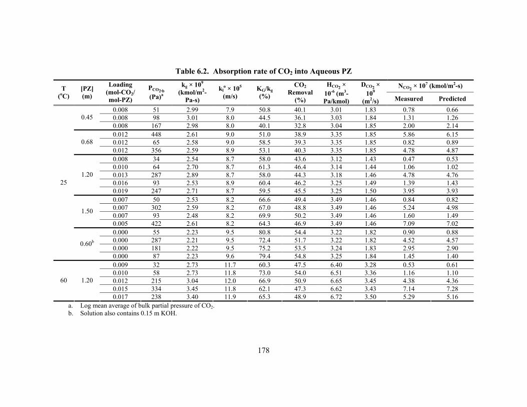
178
Table 6.2. Absorption rate of CO2 into Aqueous PZ
NCO2 × 107 (kmol/m2-s) T (oC)
[PZ] (m)
Loading (mol-CO2/ mol-PZ)
PCO2,b (Pa)a
kg × 109 (kmol/m2-
Pa-s)
klo × 105 (m/s)
KG/kg (%)
CO2 Removal
(%)
HCO2 × 10-6 (m3-Pa/kmol)
DCO2 × 109
(m2/s) Measured Predicted
0.008 51 2.99 7.9 50.8 40.1 3.01 1.83 0.78 0.66 0.008 98 3.01 8.0 44.5 36.1 3.03 1.84 1.31 1.26 0.45 0.008 167 2.98 8.0 40.1 32.8 3.04 1.85 2.00 2.14 0.012 448 2.61 9.0 51.0 38.9 3.35 1.85 5.86 6.15 0.012 65 2.58 9.0 58.5 39.3 3.35 1.85 0.82 0.89 0.68 0.012 356 2.59 8.9 53.1 40.3 3.35 1.85 4.78 4.87 0.008 34 2.54 8.7 58.0 43.6 3.12 1.43 0.47 0.53 0.010 64 2.70 8.7 61.3 46.4 3.14 1.44 1.06 1.02 0.013 287 2.89 8.7 58.0 44.3 3.18 1.46 4.78 4.76 0.016 93 2.53 8.9 60.4 46.2 3.25 1.49 1.39 1.43
1.20
0.019 247 2.71 8.7 59.5 45.5 3.25 1.50 3.95 3.93 0.007 50 2.53 8.2 66.6 49.4 3.49 1.46 0.84 0.82 0.007 302 2.59 8.2 67.0 48.8 3.49 1.46 5.24 4.98 0.007 93 2.48 8.2 69.9 50.2 3.49 1.46 1.60 1.49
1.50
0.005 422 2.61 8.2 64.3 46.9 3.49 1.46 7.09 7.02 0.000 55 2.23 9.5 80.8 54.4 3.22 1.82 0.90 0.88 0.000 287 2.21 9.5 72.4 51.7 3.22 1.82 4.52 4.57 0.000 181 2.22 9.5 75.2 53.5 3.24 1.83 2.95 2.90
25
0.60b
0.000 87 2.23 9.6 79.4 54.8 3.25 1.84 1.45 1.40 0.009 32 2.73 11.7 60.3 47.5 6.40 3.28 0.53 0.61 0.010 58 2.73 11.8 73.0 54.0 6.51 3.36 1.16 1.10 0.012 215 3.04 12.0 66.9 50.9 6.65 3.45 4.38 4.36 0.015 334 3.45 11.8 62.1 47.3 6.62 3.43 7.14 7.28
60 1.20
0.017 238 3.40 11.9 65.3 48.9 6.72 3.50 5.29 5.16 a. Log mean average of bulk partial pressure of CO2. b. Solution also contains 0.15 m KOH.
179
[PZ] (M)0.0 0.5 1.0 1.5
k 2,ap
p x 1
0-4 (m
3 /km
ol-s
)
1
10
100
25oC
40oC
60oC
0.15 KOH, 25oC
Figure 6.1. Apparent Second-Order Rate Constant for CO2 Absorption into Aqueous PZ, Lines: Model (PCO2,i = 100 Pa, kl
o = 1×10⁻⁴ m/s), Open Points: Bishnoi and Rochelle (2000), Filled Points: This Work
Data on aqueous PZ from Bishnoi (2000) and this work were combined in a
regression of PZ rate constants for CO2 absorption into aqueous PZ. The regressed
constants, reported in Table 6.1, are kPZ-PZ, kPZ-H2O, kPZ-OH, and ∆Ha. Calculated values
of the flux (Table 6.2), were within approximately 20% of the measured values. The
value of the rate constant for PZ found in this work is consistent with previous work at
similar concentrations. In 0.6 M PZ, the overall rate constant is 61,320 s-1 compared to
53,700 s-1 as given by Bishnoi. The activation energies were assumed equal for all rate
constants, with a regressed value of 33.0 kJ/mol, comparable to Bishnoi (33.6 kJ/mol).
The curves in Figure 6.1 represent a model correlation of k2,app under typical
experimental conditions. The model correlation of the experimental flux data deviates

180
by less than 25% on average. The model captures the non-first-order behavior
displayed by the experimental data and the addition of kPZ-OH effectively compensates
for the accelerated rate in the presence of excess hydroxide. The activation energy
provides an adequate fit between 25 and 60oC.
A comparison between overall rate constants of several amines at 1.0 M and
25oC is shown in Table 6.3. The fact that piperazine has the highest rate constant may
be attributed to the moderately high pKa. Also, the cyclic diamine structure yields rates
faster than would be expected from simple chemical classifications or pKa correlations.
These characteristics are also observable in diamines such as ethylenediamine and
heterocycles such as piperidine and morpholine.
Table 6.3. Overall Rate Constants for 1.0 M Amines at 25oC
Amine Sourcea (Rate/pKa)
pKa Rate Constantb
(s-1) ∆Hr
(kJ/mol) Piperazine This Work 9.73 102.2×10³ 35.0
Monoethanolamine 1/2 9.55 5.9×10³ 41.2 Diethanolamine 1/2 8.88 1.3×10³ 53.1
3/4 4.52×10³ 39.4 Diglycolamine 5/4 9.46 6.7×10³ 40.1
Ethylenediamine 6/2 9.91 15.1×10³ - 7/2 93.3×10³ - Piperidine 8/2 11.12 60.3×10³ - 3/2 20.6×10³ - 7/2 20.0×10³ - Morpholine 5/2
8.49 22.3×10³ 23.3
a. 1. Hikita et al. (1977). 2. Perrin et al. (1981). 3. Alper (1990a). 4. Littel et al. (1990a). 5. Al-Juaied (2004). 6. Jensen and Christensen (1955). 7. Sharma (1965). 8. Jensen et al. (1952).
b. Overall rate constant ( [ ] [ ] [ ]2
2 ' or Am Am Am Am H Ok k Am k Am k Am− −= + ) assuming 25oC, negligible loading, and negligible hydroxide contributions.
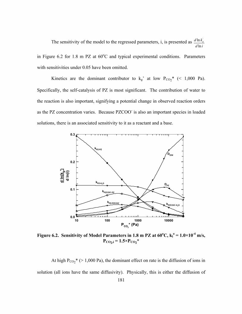
181
The sensitivity of the model to the regressed parameters, i, is presented as 'ln
lngd k
d i
in Figure 6.2 for 1.8 m PZ at 60oC and typical experimental conditions. Parameters
with sensitivities under 0.05 have been omitted.
Kinetics are the dominant contributor to kg� at low PCO2* (< 1,000 Pa).
Specifically, the self-catalysis of PZ is most significant. The contribution of water to
the reaction is also important, signifying a potential change in observed reaction orders
as the PZ concentration varies. Because PZCOO- is also an important species in loaded
solutions, there is an associated sensitivity to it as a reactant and a base.
PCO2* (Pa)
10 100 1000 10000
d ln
(kg')
d ln
(i)
0.0
0.1
0.2
0.3
kPZCOO--PZ
DION
kPZ-PZ
kPZ-H2O
kPZ-PZCOO- kPZCOO--H2O
DPZ
Figure 6.2. Sensitivity of Model Parameters in 1.8 m PZ at 60oC, kl
o = 1.0×10⁻⁴ m/s, PCO2,i = 1.5×PCO2*
At high PCO2* (> 1,000 Pa), the dominant effect on rate is the diffusion of ions in
solution (all ions have the same diffusivity). Physically, this is either the diffusion of
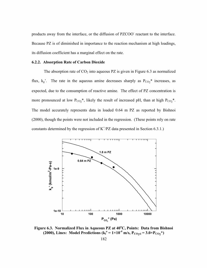
182
products away from the interface, or the diffusion of PZCOO- reactant to the interface.
Because PZ is of diminished in importance to the reaction mechanism at high loadings,
its diffusion coefficient has a marginal effect on the rate.
6.2.2. Absorption Rate of Carbon Dioxide
The absorption rate of CO2 into aqueous PZ is given in Figure 6.3 as normalized
flux, kg�. The rate in the aqueous amine decreases sharply as PCO2* increases, as
expected, due to the consumption of reactive amine. The effect of PZ concentration is
more pronounced at low PCO2*, likely the result of increased pH, than at high PCO2*.
The model accurately represents data in loaded 0.64 m PZ as reported by Bishnoi
(2000), though the points were not included in the regression. (These points rely on rate
constants determined by the regression of K+/PZ data presented in Section 6.3.1.)
PCO2* (Pa)
10 100 1000 10000
k g' (k
mol
/m2 -P
a-s)
1e-10
1e-9
1.8 m PZ
0.64 m PZ
Figure 6.3. Normalized Flux in Aqueous PZ at 40oC, Points: Data from Bishnoi
(2000), Lines: Model Predictions (klo = 1×10⁻⁴ m/s, PCO2,i = 3.0×PCO2*)
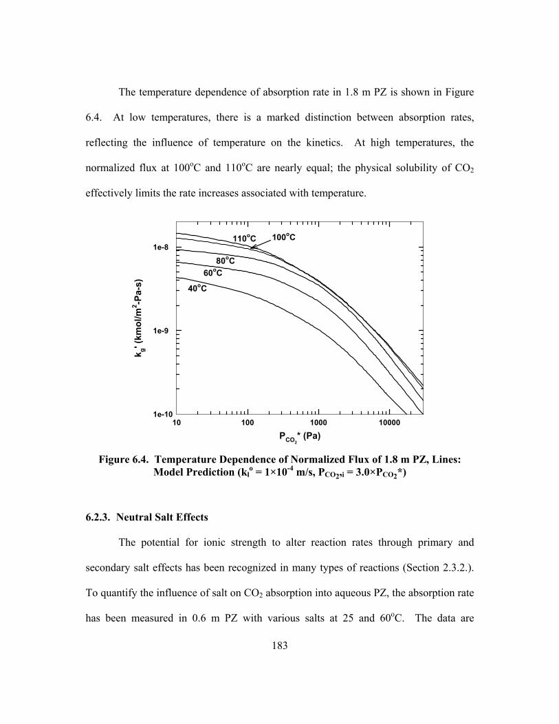
183
The temperature dependence of absorption rate in 1.8 m PZ is shown in Figure
6.4. At low temperatures, there is a marked distinction between absorption rates,
reflecting the influence of temperature on the kinetics. At high temperatures, the
normalized flux at 100oC and 110oC are nearly equal; the physical solubility of CO2
effectively limits the rate increases associated with temperature.
PCO2* (Pa)
10 100 1000 10000
k g' (k
mol
/m2 -P
a-s)
1e-10
1e-9
1e-8
40oC
60oC80oC
100oC110oC
Figure 6.4. Temperature Dependence of Normalized Flux of 1.8 m PZ, Lines:
Model Prediction (klo = 1×10⁻⁴ m/s, PCO2,i = 3.0×PCO2*)
6.2.3. Neutral Salt Effects
The potential for ionic strength to alter reaction rates through primary and
secondary salt effects has been recognized in many types of reactions (Section 2.3.2.).
To quantify the influence of salt on CO2 absorption into aqueous PZ, the absorption rate
has been measured in 0.6 m PZ with various salts at 25 and 60oC. The data are

184
presented in Table 6.4. For modeling neutral salts, the Henry�s constant of CO2 was
estimated by the model of Weisenberger and Schumpe (1996).
The salt effect is commonly represented by a function (Brønsted, 1928) so that
ln lnk k bI∞= + (6.1)
where b is a constant and I is the ionic strength. The rigorous rate model has been run
with rate constants of the form shown in Equation (6.1) to interpret the effect of neutral
salts. The average value of b was found to be 0.45 ± 0.10. The constant b can be
specific to both the ion and the reaction involved; the limited data presented here
prevent a rigorous interpretation of its value for individual species.
Other studies on ionic strength effects show similar acceleration of reaction
rates. French (1928) studied the iodine-catalyzed decomposition of hydrogen peroxide.
The influence of up to 2 M of several neutral salts increased reaction rates by as much
as factor of two. As interpreted through Equation (6.1), reported values of b include
0.32 for LiCl, 0.13 for NaCl, and 0.08 for KCl. Grube and Schmid (1926) determined
the effect of concentrated neutral salts on the hydrolysis of cyanamide. The authors
conclude that the value of b ranges from 0.16 in KNO3 to 0.40 in Mg(NO3)2. Again, the
reaction rates in 2 M ionic strength increase by a factor of two.
Neutral salts have also been shown to positively influence the absorption rate of
CO2 into amines. Data from Danckwerts and Sharma (1966) give a value for b of
approximately 0.4 for CO2 absorption into ammonia with NaCl. Laddha and
Danckwerts (1982) suggest 0.4 and 0.6 for Na2SO4 and K2SO4 in DEA respectively.
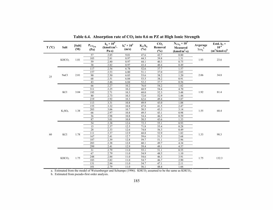
185
Table 6.4. Absorption rate of CO2 into 0.6 m PZ at High Ionic Strength
T (oC) Salt [Salt] (M)
PCO2,b (Pa)
kg × 109 (kmol/cm2-
Pa-s)
klo × 105 (m/s)
KG/kg (%)
CO2 Removal
(%)
NCO2 × 107 Measured
(kmol/m2-s)
Avgerage γCO2
a
Estd. k2 × 10-4
(m3/kmol-s)b 57 2.85 9.01 47.6 42.7 0.80
103 2.81 8.97 44.3 39.8 1.31 59 2.80 8.97 44.1 40.3 0.75
KHCO2 1.81
38 2.82 8.97 43.4 40.4 0.49
1.93 23.6
117 2.54 6.78 52.6 37.7 1.57 157 2.53 6.80 51.1 37.0 2.03 90 2.50 6.83 53.6 38.2 1.20 68 2.51 6.84 53.5 38.2 0.91
NaCl 2.81
43 2.46 6.84 52.2 37.7 0.56
2.06 34.8
66 2.27 10.2 76.0 54.2 1.02 311 2.25 10.2 68.9 54.4 4.70 195 2.71 10.3 68.0 52.3 3.48 80 2.73 10.3 72.0 52.9 1.44
25
KCl 3.04
219 2.92 10.3 62.6 49.4 3.87
1.92 81.4
113 3.31 10.8 49.9 43.0 1.88 155 3.32 10.8 47.8 41.5 2.47 203 3.06 10.7 50.5 43.3 3.14 66 2.97 10.8 49.5 43.1 0.98 36 2.98 10.8 54.4 46.5 0.59
K2SO4 1.38
87 3.01 10.8 50.5 43.6 1.33
1.55 68.4
54 2.38 12.6 72.3 55.1 0.93 15 2.37 12.5 71.8 55.4 0.28 28 2.33 12.6 74.8 56.3 0.49
111 2.37 12.9 68.8 52.9 1.82 167 2.41 12.7 59.6 51.5 2.68 187 2.39 12.8 59.7 51.1 2.96 283 2.38 12.8 60.1 49.7 4.34
KCl 1.78
299 2.41 12.9 59.4 49.1 4.57
1.33 98.3
31 2.79 11.0 55.1 51.1 0.55 67 2.79 11.0 54.9 48.5 1.10
248 2.84 11.0 54.6 46.3 3.91 183 2.82 11.0 54.7 46.7 2.90 131 2.84 11.0 54.7 47.1 2.11
60
KHCO2 1.75
101 2.79 11.0 56.1 48.4 1.66
1.75 132.3
a. Estimated from the model of Weisenberger and Schumpe (1996). KHCO2 assumed to be the same as KHCO3. b. Estimated from pseudo-first order analysis.
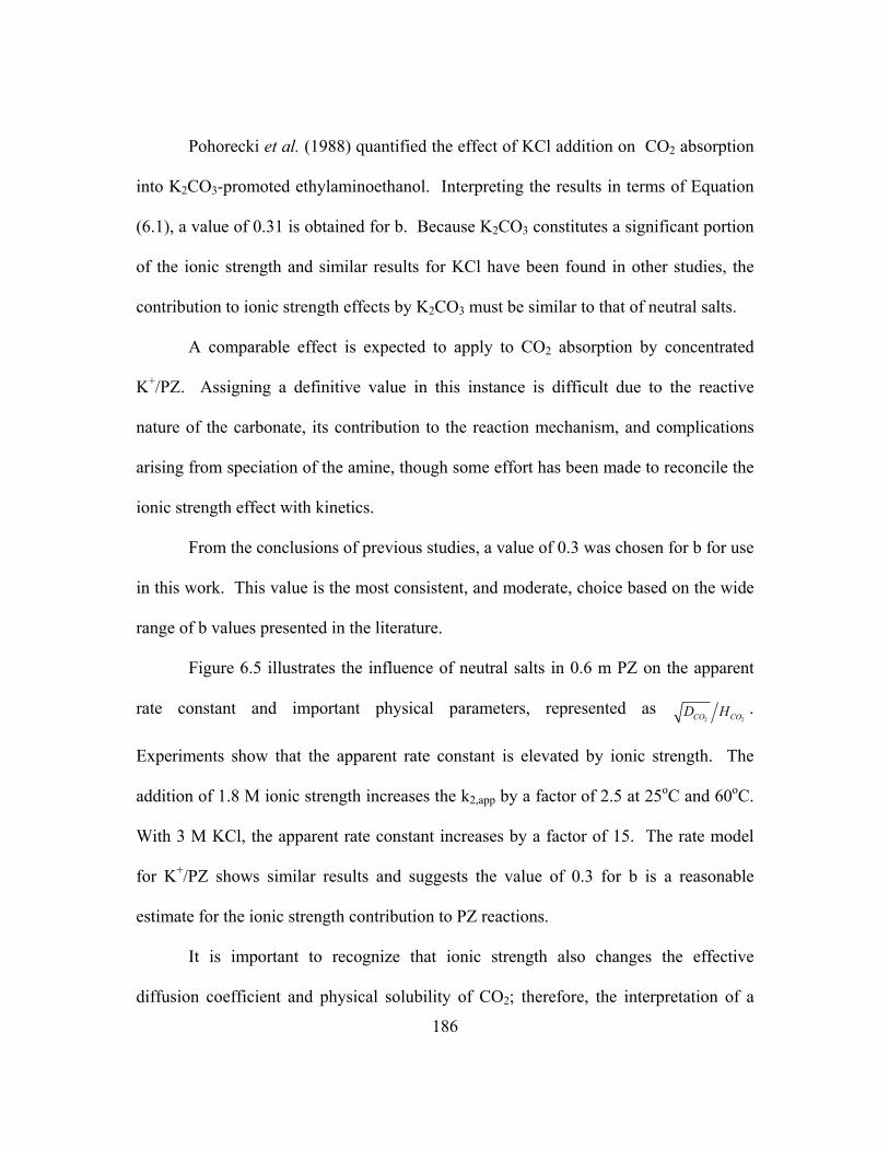
186
Pohorecki et al. (1988) quantified the effect of KCl addition on CO2 absorption
into K2CO3-promoted ethylaminoethanol. Interpreting the results in terms of Equation
(6.1), a value of 0.31 is obtained for b. Because K2CO3 constitutes a significant portion
of the ionic strength and similar results for KCl have been found in other studies, the
contribution to ionic strength effects by K2CO3 must be similar to that of neutral salts.
A comparable effect is expected to apply to CO2 absorption by concentrated
K+/PZ. Assigning a definitive value in this instance is difficult due to the reactive
nature of the carbonate, its contribution to the reaction mechanism, and complications
arising from speciation of the amine, though some effort has been made to reconcile the
ionic strength effect with kinetics.
From the conclusions of previous studies, a value of 0.3 was chosen for b for use
in this work. This value is the most consistent, and moderate, choice based on the wide
range of b values presented in the literature.
Figure 6.5 illustrates the influence of neutral salts in 0.6 m PZ on the apparent
rate constant and important physical parameters, represented as 2 2CO COD H .
Experiments show that the apparent rate constant is elevated by ionic strength. The
addition of 1.8 M ionic strength increases the k2,app by a factor of 2.5 at 25oC and 60oC.
With 3 M KCl, the apparent rate constant increases by a factor of 15. The rate model
for K+/PZ shows similar results and suggests the value of 0.3 for b is a reasonable
estimate for the ionic strength contribution to PZ reactions.
It is important to recognize that ionic strength also changes the effective
diffusion coefficient and physical solubility of CO2; therefore, the interpretation of a
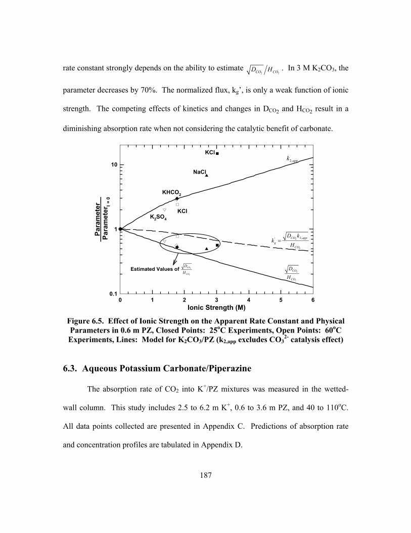
187
rate constant strongly depends on the ability to estimate 2 2CO COD H . In 3 M K2CO3, the
parameter decreases by 70%. The normalized flux, kg�, is only a weak function of ionic
strength. The competing effects of kinetics and changes in DCO2 and HCO2 result in a
diminishing absorption rate when not considering the catalytic benefit of carbonate.
Ionic Strength (M)0 1 2 3 4 5 6
Pa
ram
eter
P
aram
eter
I = 0
0.1
1
10
KHCO2
NaCl
KCl
KClK2SO4
2
2
CO
CO
D
H
2
2
2,' CO appg
CO
D kk
H=
2,appk
Estimated Values of 2
2
CO
CO
D
H
Figure 6.5. Effect of Ionic Strength on the Apparent Rate Constant and Physical Parameters in 0.6 m PZ, Closed Points: 25oC Experiments, Open Points: 60oC Experiments, Lines: Model for K2CO3/PZ (k2,app excludes CO3
2- catalysis effect)
6.3. Aqueous Potassium Carbonate/Piperazine
The absorption rate of CO2 into K+/PZ mixtures was measured in the wetted-
wall column. This study includes 2.5 to 6.2 m K+, 0.6 to 3.6 m PZ, and 40 to 110oC.
All data points collected are presented in Appendix C. Predictions of absorption rate
and concentration profiles are tabulated in Appendix D.
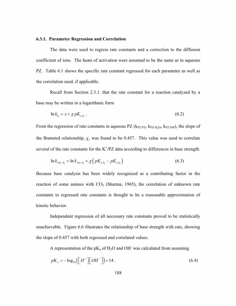
188
6.3.1. Parameter Regression and Correlation
The data were used to regress rate constants and a correction to the diffusion
coefficient of ions. The heats of activation were assumed to be the same as in aqueous
PZ. Table 6.1 shows the specific rate constant regressed for each parameter as well as
the correlation used, if applicable.
Recall from Section 2.3.1. that the rate constant for a reaction catalyzed by a
base may be written in a logarithmic form
1 1,ln b a bk x pKχ= + . (6.2)
From the regression of rate constants in aqueous PZ (kPZ-PZ, kPZ-H2O, kPZ-OH), the slope of
the Brønsted relationship, χ, was found to be 0.457. This value was used to correlate
several of the rate constants for the K+/PZ data according to differences in base strength.
( )2 1 2 1, ,ln lnAm b Am b a b a bk k pK pKχ− −= + − (6.3)
Because base catalysis has been widely recognized as a contributing factor in the
reaction of some amines with CO2 (Sharma, 1965), the correlation of unknown rate
constants to regressed rate constants is thought to be a reasonable approximation of
kinetic behavior.
Independent regression of all necessary rate constants proved to be statistically
unachievable. Figure 6.6 illustrates the relationship of base strength with rate, showing
the slope of 0.457 with both regressed and correlated values.
A representation of the pKa of H2O and OH- was calculated from assuming
( )10log 14wpK H OH+ − = − = . (6.4)
189
Thus,
[ ]10,2
log 15.74a OH
H OHpK
H O−
+ − = − =
, (6.5)
and
2, , ,1.74a H O a w a OH
pK pK pK −= − = − . (6.6)
pKa,base
-2 0 2 4 6 8 10 12 14 16
ln k
Am-b
o ( m6 /k
mol
2 -s)
5
10
15
kPZ-PZCOO-
kPZ-H2O
kPZ-CO32-
kPZCOO--PZCOO-
kPZ-PZ
kPZCOO--H2O
kPZCOO--CO32-
kPZ-OH-
kPZCOO--PZ
Figure 6.6. Fit of Specific Rate Constants to Brønsted Theory of Acid-Basic Catalysis, Circles: Independently Regressed, Squares: Correlated by Slope
This type of approximation is supported by previous work on other amines.
Data on CO2 absorption into aqueous morpholine (MOR), diethanolamine (DEA), and
diisopropanolamine (DIPA) have been reanalyzed in terms of a termolecular
mechanism to give rate constants for comparison to PZ in this work. The rate constants
are presented in Figure 6.7 and Table 6.5.
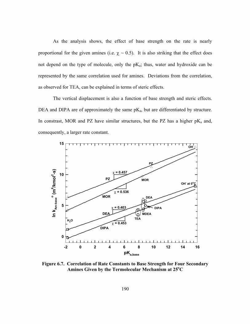
190
As the analysis shows, the effect of base strength on the rate is nearly
proportional for the given amines (i.e. χ ~ 0.5). It is also striking that the effect does
not depend on the type of molecule, only the pKa; thus, water and hydroxide can be
represented by the same correlation used for amines. Deviations from the correlation,
as observed for TEA, can be explained in terms of steric effects.
The vertical displacement is also a function of base strength and steric effects.
DEA and DIPA are of approximately the same pKa, but are differentiated by structure.
In constrast, MOR and PZ have similar structures, but the PZ has a higher pKa and,
consequently, a larger rate constant.
pKa,base
-2 0 2 4 6 8 10 12 14 16
ln k
Am-b
aseo ( m
6 /km
ol2 -s
)
0
5
10
15
PZ
DIPA
DEA
PZ
H2OTEA
OH-
DIPA
MDEA
DEA
χ = 0.457
χ = 0.453
χ = 0.403
MOR
MOR
χ = 0.536
OH- at 0oC
Figure 6.7. Correlation of Rate Constants to Base Strength for Four Secondary
Amines Given by the Termolecular Mechanism at 25oC
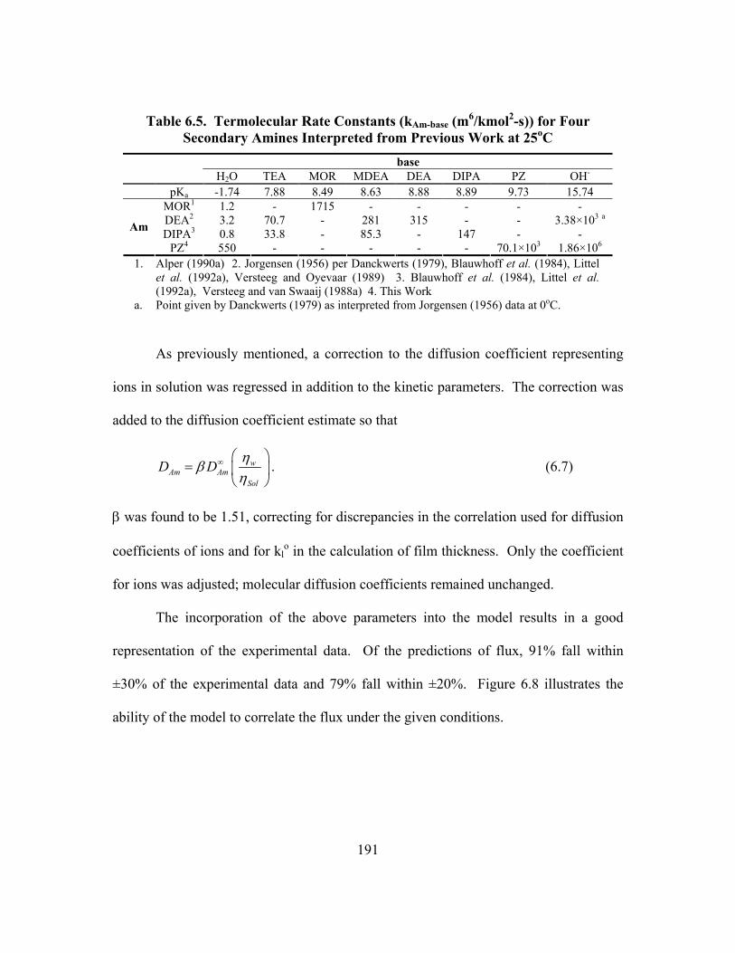
191
Table 6.5. Termolecular Rate Constants (kAm-base (m6/kmol2-s)) for Four Secondary Amines Interpreted from Previous Work at 25oC
base H2O TEA MOR MDEA DEA DIPA PZ OH- pKa -1.74 7.88 8.49 8.63 8.88 8.89 9.73 15.74
MOR1 1.2 - 1715 - - - - - DEA2 3.2 70.7 - 281 315 - - 3.38×10³ a DIPA3 0.8 33.8 - 85.3 - 147 - - Am
PZ4 550 - - - - - 70.1×10³ 1.86×10⁶ 1. Alper (1990a) 2. Jorgensen (1956) per Danckwerts (1979), Blauwhoff et al. (1984), Littel
et al. (1992a), Versteeg and Oyevaar (1989) 3. Blauwhoff et al. (1984), Littel et al. (1992a), Versteeg and van Swaaij (1988a) 4. This Work
a. Point given by Danckwerts (1979) as interpreted from Jorgensen (1956) data at 0oC.
As previously mentioned, a correction to the diffusion coefficient representing
ions in solution was regressed in addition to the kinetic parameters. The correction was
added to the diffusion coefficient estimate so that
wAm Am
Sol
D D ηβη
∞ =
. (6.7)
β was found to be 1.51, correcting for discrepancies in the correlation used for diffusion
coefficients of ions and for klo in the calculation of film thickness. Only the coefficient
for ions was adjusted; molecular diffusion coefficients remained unchanged.
The incorporation of the above parameters into the model results in a good
representation of the experimental data. Of the predictions of flux, 91% fall within
±30% of the experimental data and 79% fall within ±20%. Figure 6.8 illustrates the
ability of the model to correlate the flux under the given conditions.
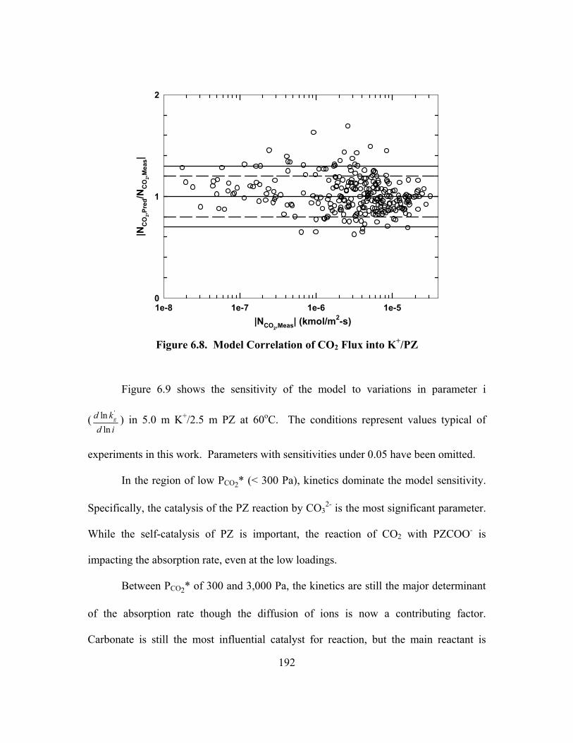
192
|NCO2,Meas| (kmol/m2-s)1e-8 1e-7 1e-6 1e-5
|NC
O2,P
red/N
CO
2,Mea
s|
0
1
2
Figure 6.8. Model Correlation of CO2 Flux into K+/PZ
Figure 6.9 shows the sensitivity of the model to variations in parameter i
('ln
lngd k
d i) in 5.0 m K+/2.5 m PZ at 60oC. The conditions represent values typical of
experiments in this work. Parameters with sensitivities under 0.05 have been omitted.
In the region of low PCO2* (< 300 Pa), kinetics dominate the model sensitivity.
Specifically, the catalysis of the PZ reaction by CO32- is the most significant parameter.
While the self-catalysis of PZ is important, the reaction of CO2 with PZCOO- is
impacting the absorption rate, even at the low loadings.
Between PCO2* of 300 and 3,000 Pa, the kinetics are still the major determinant
of the absorption rate though the diffusion of ions is now a contributing factor.
Carbonate is still the most influential catalyst for reaction, but the main reactant is
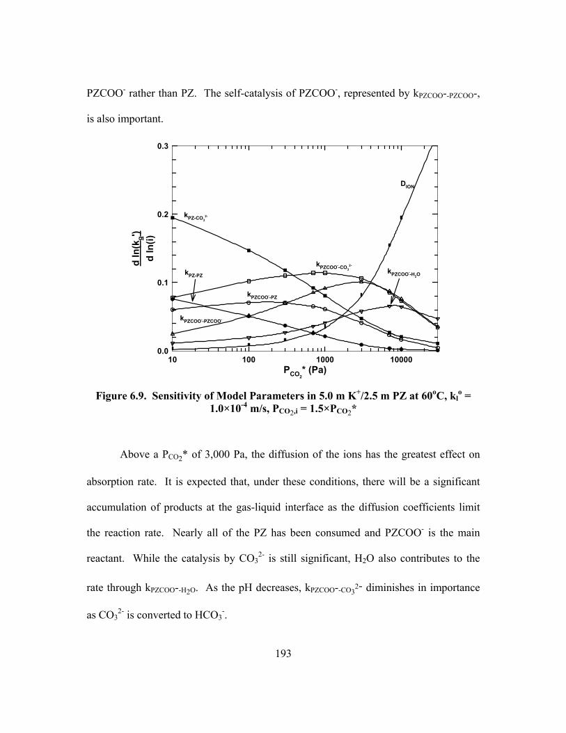
193
PZCOO- rather than PZ. The self-catalysis of PZCOO-, represented by kPZCOO--PZCOO-,
is also important.
PCO2* (Pa)
10 100 1000 10000
d ln
(kg')
d ln
(i)
0.0
0.1
0.2
0.3
kPZCOO--PZ
DION
kPZ-PZ
kPZCOO--CO32-
kPZ-CO32-
kPZCOO--PZCOO-
kPZCOO--H2O
Figure 6.9. Sensitivity of Model Parameters in 5.0 m K+/2.5 m PZ at 60oC, kl
o = 1.0×10⁻⁴ m/s, PCO2,i = 1.5×PCO2*
Above a PCO2* of 3,000 Pa, the diffusion of the ions has the greatest effect on
absorption rate. It is expected that, under these conditions, there will be a significant
accumulation of products at the gas-liquid interface as the diffusion coefficients limit
the reaction rate. Nearly all of the PZ has been consumed and PZCOO- is the main
reactant. While the catalysis by CO32- is still significant, H2O also contributes to the
rate through kPZCOO--H2O. As the pH decreases, kPZCOO--CO32- diminishes in importance
as CO32- is converted to HCO3
-.

194
In addition to discerning common trends for model sensitivity, Figure 6.9 also
highlights the complexity of regressing parameters within a multi-parameter reaction
mechanism. It is typical for several parameters to have approximately the same
significance under similar conditions. In these cases, independent regression of these
parameters is difficult and a method of correlating the values may be justified.
6.3.2. Absorption Rate of Carbon Dioxide
Given the ability of the model to represent the experimental data accurately, it is
useful to compare model correlations to arrive at conclusions concerning solvent
performance at various conditions. Solvent concentrations and temperature dependence
are of particular interest as these properties often dictate overall performance.
The normalized flux (kg�) of several K+/PZ solvents is shown in Figure 6.10. In
promoted K2CO3 (i.e. 3.6 m K+/0.6 m PZ), the absorption rate is fast, though 20 to 30%
less than 5 M MEA under similar conditions. More concentrated solvents, such as 3.6
m K+/1.8 m PZ, have absorption rates a factor of 2 higher than the promoted solvent and
a factor of 1.5 higher than 5 M MEA. The 3.6 m K+/3.6 m PZ solvent has an absorption
rate 2 to 3 times that of 5 M MEA. From Section 5.6, this solvent is expected to have a
high capacity; however, volatility may prevent concentrated PZ solvents from being
commercially viable.
Interestingly, 5.0 m K+/2.5 m PZ has a normalized flux nearly identical to 3.6 m
K+/1.8 m PZ. The similarity can be explained by two mechanisms. First, in the
concentrated solvents, the viscosity is higher, leading to smaller diffusion coefficients.
Second, the physical solubility of CO2 is less in the higher ionic strength environment.

195
The competing effects of kinetics and diffusivity and solubility appear to play a
significant role in determining the absorption rate in some concentrated solvents.
PCO2* (Pa)
10 100 1000 10000
k g' (k
mol
/m2 -P
a-s)
1e-9
3.6 m K+/3.6 m PZ
3.6 m K+/0.6 m PZ3.6 m K+/1.8 m PZ
5.0 m K+/2.5 m PZ
7 m MEA
Figure 6.10. Normalized Flux in K+/PZ Mixtures at 60oC, Points: Experimental
Data (MEA from Dang (2001)), Lines: Model Prediction (klo = 1×10⁻⁴ m/s, PCO2,i =
3.0×PCO2*)
The relative impact of K+ and PZ on the absorption rate is compared in Figure
6.11. The two lines demonstrate the changing ratio of K+:PZ where one component is
constant. As the amount of PZ increases relative to the K+ concentration, an increase in
the rate of absorption is observed in both the cases of constant K+ and constant PZ.
From a K+:PZ ratio of 8:1 to 1:1, the normalized flux increases by a factor of three.
As suggested previously, more concentrated solvents do not necessarily yield
faster absorption rates. This is somewhat unexpected since previous investigations of
speciation suggest more reactive species are present at higher total solvent
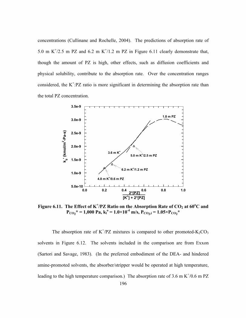
196
concentrations (Cullinane and Rochelle, 2004). The predictions of absorption rate of
5.0 m K+/2.5 m PZ and 6.2 m K+/1.2 m PZ in Figure 6.11 clearly demonstrate that,
though the amount of PZ is high, other effects, such as diffusion coefficients and
physical solubility, contribute to the absorption rate. Over the concentration ranges
considered, the K+:PZ ratio is more significant in determining the absorption rate than
the total PZ concentration.
2*[PZ] [K+] + 2*[PZ]
0.0 0.2 0.4 0.6 0.8 1.0
k g' (k
mol
/m2 -P
a-s)
5.0e-10
1.0e-9
1.5e-9
2.0e-9
2.5e-9
3.0e-9
3.5e-9
1.8 m PZ
3.6 m K+
5.0 m K+/2.5 m PZ
4.8 m K+/0.6 m PZ
6.2 m K+/1.2 m PZ
Figure 6.11. The Effect of K+/PZ Ratio on the Absorption Rate of CO2 at 60oC and
PCO2* = 1,000 Pa, klo = 1.0×10⁻⁴ m/s, PCO2,i = 1.05×PCO2*
The absorption rate of K+/PZ mixtures is compared to other promoted-K2CO3
solvents in Figure 6.12. The solvents included in the comparison are from Exxon
(Sartori and Savage, 1983). (In the preferred embodiment of the DEA- and hindered
amine-promoted solvents, the absorber/stripper would be operated at high temperature,
leading to the high temperature comparison.) The absorption rate of 3.6 m K+/0.6 m PZ
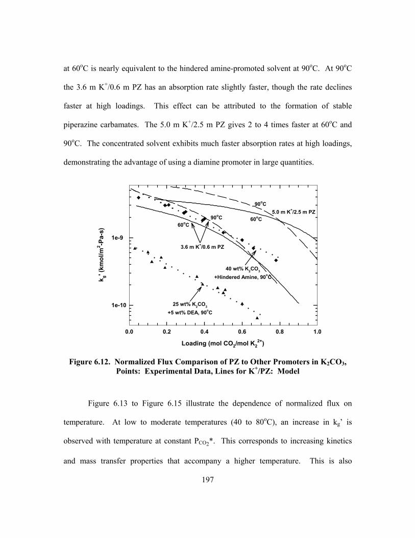
197
at 60oC is nearly equivalent to the hindered amine-promoted solvent at 90oC. At 90oC
the 3.6 m K+/0.6 m PZ has an absorption rate slightly faster, though the rate declines
faster at high loadings. This effect can be attributed to the formation of stable
piperazine carbamates. The 5.0 m K+/2.5 m PZ gives 2 to 4 times faster at 60oC and
90oC. The concentrated solvent exhibits much faster absorption rates at high loadings,
demonstrating the advantage of using a diamine promoter in large quantities.
Loading (mol CO2/mol K22+)
0.0 0.2 0.4 0.6 0.8 1.0
k g' (k
mol
/m2 -P
a-s)
1e-10
1e-9
25 wt% K2CO3
+5 wt% DEA, 90oC
3.6 m K+/0.6 m PZ
40 wt% K2CO3
+Hindered Amine, 90oC
5.0 m K+/2.5 m PZ60oC
90oC
60oC90oC
Figure 6.12. Normalized Flux Comparison of PZ to Other Promoters in K2CO3,
Points: Experimental Data, Lines for K+/PZ: Model
Figure 6.13 to Figure 6.15 illustrate the dependence of normalized flux on
temperature. At low to moderate temperatures (40 to 80oC), an increase in kg� is
observed with temperature at constant PCO2*. This corresponds to increasing kinetics
and mass transfer properties that accompany a higher temperature. This is also
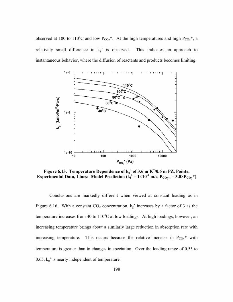
198
observed at 100 to 110oC and low PCO2*. At the high temperatures and high PCO2*, a
relatively small difference in kg� is observed. This indicates an approach to
instantaneous behavior, where the diffusion of reactants and products becomes limiting.
PCO2* (Pa)
10 100 1000 10000
k g' (k
mol
/m2 -P
a-s)
1e-10
1e-9
1e-8
40oC
60oC80oC
100oC
110oC
Figure 6.13. Temperature Dependence of kg� of 3.6 m K+/0.6 m PZ, Points:
Experimental Data, Lines: Model Prediction (klo = 1×10⁻⁴ m/s, PCO2,i = 3.0×PCO2*)
Conclusions are markedly different when viewed at constant loading as in
Figure 6.16. With a constant CO2 concentration, kg� increases by a factor of 3 as the
temperature increases from 40 to 110oC at low loadings. At high loadings, however, an
increasing temperature brings about a similarly large reduction in absorption rate with
increasing temperature. This occurs because the relative increase in PCO2* with
temperature is greater than in changes in speciation. Over the loading range of 0.55 to
0.65, kg� is nearly independent of temperature.
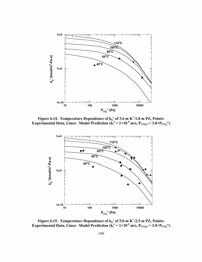
199
PCO2* (Pa)
10 100 1000 10000
k g' (k
mol
/m2 -P
a-s)
1e-10
1e-9
1e-8
40oC
60oC80oC
100oC110oC
Figure 6.14. Temperature Dependence of kg� of 3.6 m K+/1.8 m PZ, Points:
Experimental Data, Lines: Model Prediction (klo = 1×10⁻⁴ m/s, PCO2,i = 3.0×PCO2*)
PCO2* (Pa)
10 100 1000 10000
k g' (k
mol
/m2 -P
a-s)
1e-10
1e-9
1e-8
40oC
60oC
80oC100oC
110oC
Figure 6.15. Temperature Dependence of kg� of 5.0 m K+/2.5 m PZ, Points:
Experimental Data, Lines: Model Prediction (klo = 1×10⁻⁴ m/s, PCO2,i = 3.0×PCO2*)
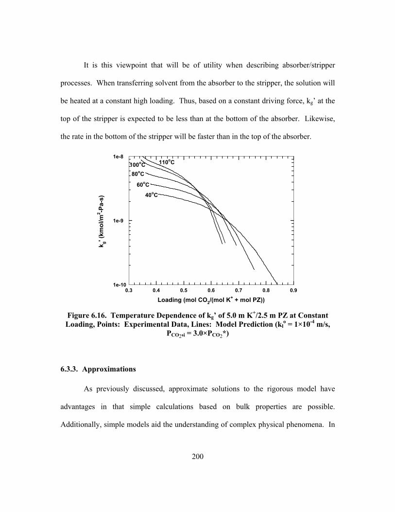
200
It is this viewpoint that will be of utility when describing absorber/stripper
processes. When transferring solvent from the absorber to the stripper, the solution will
be heated at a constant high loading. Thus, based on a constant driving force, kg� at the
top of the stripper is expected to be less than at the bottom of the absorber. Likewise,
the rate in the bottom of the stripper will be faster than in the top of the absorber.
Loading (mol CO2/(mol K+ + mol PZ))0.3 0.4 0.5 0.6 0.7 0.8 0.9
k g' (k
mol
/m2 -P
a-s)
1e-10
1e-9
1e-8
40oC
60oC
80oC100oC 110oC
Figure 6.16. Temperature Dependence of kg� of 5.0 m K+/2.5 m PZ at Constant Loading, Points: Experimental Data, Lines: Model Prediction (kl
o = 1×10⁻⁴ m/s, PCO2,i = 3.0×PCO2*)
6.3.3. Approximations
As previously discussed, approximate solutions to the rigorous model have
advantages in that simple calculations based on bulk properties are possible.
Additionally, simple models aid the understanding of complex physical phenomena. In
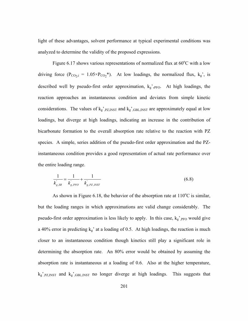
201
light of these advantages, solvent performance at typical experimental conditions was
analyzed to determine the validity of the proposed expressions.
Figure 6.17 shows various representations of normalized flux at 60oC with a low
driving force (PCO2,i = 1.05×PCO2*). At low loadings, the normalized flux, kg�, is
described well by pseudo-first order approximation, kg�,PFO. At high loadings, the
reaction approaches an instantaneous condition and deviates from simple kinetic
considerations. The values of kg�,PZ,INST and kg�,GBL,INST are approximately equal at low
loadings, but diverge at high loadings, indicating an increase in the contribution of
bicarbonate formation to the overall absorption rate relative to the reaction with PZ
species. A simple, series addition of the pseudo-first order approximation and the PZ-
instantaneous condition provides a good representation of actual rate performance over
the entire loading range.
' ' ', , , ,
1 1 1
g SR g PFO g PZ INSTk k k= + (6.8)
As shown in Figure 6.18, the behavior of the absorption rate at 110oC is similar,
but the loading ranges in which approximations are valid change considerably. The
pseudo-first order approximation is less likely to apply. In this case, kg�,PFO would give
a 40% error in predicting kg� at a loading of 0.5. At high loadings, the reaction is much
closer to an instantaneous condition though kinetics still play a significant role in
determining the absorption rate. An 80% error would be obtained by assuming the
absorption rate is instantaneous at a loading of 0.6. Also at the higher temperature,
kg�,PZ,INST and kg�,GBL,INST no longer diverge at high loadings. This suggests that
202
reactions to form bicarbonate are sufficiently fast due to increased temperature that they
may be considered instantaneous.
Loading (mol CO2/(mol K+ + mol PZ))0.45 0.50 0.55 0.60 0.65 0.70 0.75
k g' (k
mol
/m2 -P
a-s)
1e-10
1e-9
1e-8
1e-7
kg',PZ,INST
kg',PFO
kg'
kg',SR
kg',GBL,INST
100 Pa 10,000 Pa1,000 Pa
Figure 6.17. Approximate Solutions to Normalized Flux in 5.0 m K+/2.5 m PZ at
60oC, klo = 1.0×10⁻⁴ m/s, PCO2,i = 1.05×PCO2*
The previous examples illustrate the usefulness of approximations under low
driving force conditions. With the imposition of a large driving force, the transport of
species becomes less empirical and simple representations may break down. Figure
6.19 demonstrates that the simple, series resistance model is not a satisfactory
representation at higher driving forces. Much of the inaccuracies fall in the high
loading region where equilibrium effects, not pseudo-first order conditions, must
change across the boundary layer.

203
Loading (mol CO2/(mol K+ + mol PZ))0.45 0.50 0.55 0.60 0.65 0.70 0.75
k g' (k
mol
/m2 -P
a-s)
1e-10
1e-9
1e-8
1e-7
kg',PZ,INST and kg',GBL,INST
kg',PFOkg'
kg',SR
1,000 Pa 10,000 Pa 100,000 Pa
Figure 6.18. Approximate Solutions to Normalized Flux in 5.0 m K+/2.5 m PZ at
110oC, klo = 1.0×10⁻⁴ m/s, PCO2,i = 1.05×PCO2*
Loading (mol CO2/(mol K+ + mol PZ))0.45 0.50 0.55 0.60 0.65 0.70 0.75
k g' (k
mol
/m2 -P
a-s)
1e-10
1e-9
kg',PFO
kg',SR
kg',PCO2,i = 10xPCO2
*
100 Pa 10,000 Pa1,000 Pa
kg',PCO2,i = 3xPCO2
*
Figure 6.19. Effect of Driving Force on Approximate Solutions to Normalized Flux
in 5.0 m K+/2.5 m PZ at 60oC, klo = 1.0×10⁻⁴ m/s

204
The analysis presented in Table 6.6 shows the difficulty. The ability to
represent the absorption rate empirically based on bulk solution properties rests on the
change in species concentrations across the interface. At low loadings and low and high
temperatures, the absorption rate can be still described by the pseudo-first order
approximation even with a factor of 10 driving force. At 110oC and a loading of 0.473,
the concentrations of PZ and PZCOO- change by less than 5% across the boundary
layer; however, substantial differences in the buffering species carbonate and
bicarbonate are predicted. This indicates a changing equilibrium across the boundary
layer and shows that an equilibrium representation of instantaneous behavior is not
sufficient.
Table 6.6. Concentration (kmol/m3) Across the Liquid Boundary Layer in 5.0 m K+/2.5 m PZ, kl
o = 1.0x10⁻⁴ m/s
PCO2,i = 10.0×PCO2*, T = 60oC PCO2,i = 0.1×PCO2*, T = 110oC Loadinga 0.473 0.586 0.473 0.586
PCO2* (Pa) 100 1,000 810 7,600 Interface Bulk Interface Bulk Interface Bulk Interface Bulk
CO32- 1.155 1.179 0.518 0.633 1.161 1.118 0.644 0.479
HCO3- 0.281 0.258 0.663 0.548 0.299 0.340 0.469 0.624
PZ 0.810 0.831 0.26 0.344 0.965 0.931 0.547 0.447 PZH+ 0.019 0.017 0.07 0.062 0.002 0.002 0.006 0.009
PZCOO- 0.863 0.859 0.671 0.733 0.700 0.711 0.659 0.638 H+PZCOO- 0.027 0.024 0.143 0.106 0.003 0.003 0.008 0.014 PZ(COO-)2 0.248 0.237 0.771 0.679 0.268 0.286 0.682 0.781 a. Loading given in mol CO2/(mol K+ + mol PZ)
At high loadings, substantial differences in concentrations are obtained for most
of the species; simple models based on bulk solution equilibrium will not describe the
absorption rate. At 60oC, PZ and PZCOO- are depleted by 24% and 9% respectively.
Also, an accumulation (or depletion) of PZ(COO-)2 occurs at the interface. Although

205
PZH+ and H+PZCOO- are accumulating to a notable extent, most of the buffering still
occurs with the CO32-/HCO3
-.
Figure 6.20 illustrates changes in the liquid boundary layer as a result of
approaching instantaneous behavior. Under kinetically controlled conditions (60oC and
PCO2,i = 10.0×PCO2*), the influence of chemical reaction is apparent in the large region
of nonlinear approach to the interface concentration of CO2 near the interface (r < 0.01).
Further away (r > 0.01), the profile is linear, extending to the equilibrium concentration
of CO2 in the bulk solution, [CO2]b. Only 10% of the mass transfer occurs in the linear
diffusion region, whereas 90% occurs as a result of reaction with amines near the
interface.
r (Dimensionless Distance from Interface)0.000 0.002 0.004 0.006 0.008 0.010
[CO
2] (m
ol/m
3 )
0.00
0.05
0.10
0.15
0.20
0.25
0.30
0.35
[CO2]b,110oC
[CO2]b,60oC
[CO2]60oC
[CO2]110oC
Figure 6.20. Concentration Profile in 5.0 m K+/2.5 m PZ, Loading = 0.586 mol
CO2/(mol K+ + mol PZ), (PCO2* = 1,000 Pa at 60oC), klo = 1.0×10⁻⁴ m/s, Solid Line:
PCO2,i = 10.0×PCO2* and T = 60oC, Dashed Line: PCO2,i = 0.1×PCO2* and T = 110oC
206
The mass transfer characteristics change dramatically at high temperatures as
instantaneous conditions are approached. At 110oC and PCO2,i = 0.1×PCO2*, the zone of
chemical reaction is much closer to the interface, terminating at r = 0.001. Now, 58%
of the mass transfer occurs in the diffusion boundary layer and 42% in the reaction
zone. In this case, diffusion of reactants and products has become much more
significant in determining the absorption rate.
6.3.4. Applications
A useful function of the fundamental modeling provided by this work is its
application to estimating the behavior of the K+/PZ solvent under typical industrial
conditions. As an exercise, the solvent performance was analyzed under conditions that
may be encountered in treating flue gas from a coal-fired power plant.
Figure 6.21 shows the calculated kg� with a low driving force and a variation of
klo. The wetted-wall column in this work typically operates at a kl
o of 10-4 m/s, which is
in the pseudo-first order region under most conditions. Low values of klo, as would be
typical of quiescent liquids, result in a sharply decreasing kg� as the reaction moves into
the instantaneous region. At 60oC, the transition occurs at approximately 2×10⁻⁵ m/s.
The difference in kg� with temperature in the instantaneous region is a function of
equilibrium at the given conditions. Increasing the value of klo from pseudo-first order
conditions yields a transition to physical absorption. This occurs at very large klo (i.e. >
0.1 m/s) indicative of rapid mixing of the fluid. The difference in temperature in the
physical mass transfer region is a result of the physical solubility of CO2.
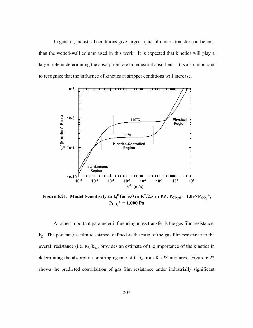
207
In general, industrial conditions give larger liquid film mass transfer coefficients
than the wetted-wall column used in this work. It is expected that kinetics will play a
larger role in determining the absorption rate in industrial absorbers. It is also important
to recognize that the influence of kinetics at stripper conditions will increase.
klo (m/s)
10-6 10-5 10-4 10-3 10-2 10-1 100 101
k g' (k
mol
/m2 -P
a-s)
1e-10
1e-9
1e-8
1e-7
60oC
110oC
InstantaneousRegion
Kinetics-ControlledRegion
PhysicalRegion
Figure 6.21. Model Sensitivity to kl
o for 5.0 m K+/2.5 m PZ, PCO2,i = 1.05×PCO2*, PCO2* = 1,000 Pa
Another important parameter influencing mass transfer is the gas film resistance,
kg. The percent gas film resistance, defined as the ratio of the gas film resistance to the
overall resistance (i.e. KG/kg), provides an estimate of the importance of the kinetics in
determining the absorption or stripping rate of CO2 from K+/PZ mixtures. Figure 6.22
shows the predicted contribution of gas film resistance under industrially significant
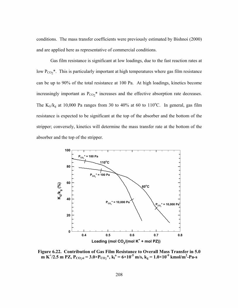
208
conditions. The mass transfer coefficients were previously estimated by Bishnoi (2000)
and are applied here as representative of commercial conditions.
Gas film resistance is significant at low loadings, due to the fast reaction rates at
low PCO2*. This is particularly important at high temperatures where gas film resistance
can be up to 90% of the total resistance at 100 Pa. At high loadings, kinetics become
increasingly important as PCO2* increases and the effective absorption rate decreases.
The KG/kg at 10,000 Pa ranges from 30 to 40% at 60 to 110oC. In general, gas film
resistance is expected to be significant at the top of the absorber and the bottom of the
stripper; conversely, kinetics will determine the mass transfer rate at the bottom of the
absorber and the top of the stripper.
Loading (mol CO2/(mol K+ + mol PZ))0.4 0.5 0.6 0.7 0.8
KG/k
g (%
)
0
20
40
60
80
100
110oC
60oC
PCO2* = 100 Pa
PCO2* = 100 Pa
PCO2* = 10,000 Pa
PCO2* = 10,000 Pa
Figure 6.22. Contribution of Gas Film Resistance to Overall Mass Transfer in 5.0
m K+/2.5 m PZ, PCO2,i = 3.0×PCO2*, klo = 6×10⁻⁵ m/s, kg = 1.0×10⁻⁹ kmol/m2-Pa-s

209
6.4. Conclusions
Investigations on the rate of CO2 absorption into aqueous PZ reveal that the
reaction can approach second-order with respect to PZ. The addition of 0.15 m KOH
increases the absorption rate in 0.6 m PZ by a factor of 2, suggesting that strong bases
must be included in the reaction mechanism. The kinetics can be represented by both
the �zwitterion� and termolecular mechanisms.
The rigorous rate model was used to regress rate constants to describe aqueous
PZ. The values are consistent with the Brønsted theory of base catalysis and with
behavior of other amine studies. The apparent rate constant of 1 M PZ is a factor of 20
greater than MEA and a factor of 100 greater than DEA. The rapid reaction of the PZ
with CO2 can be attributed to its unique, cyclic diamine structure.
Neutral salts in aqueous PZ significantly influence the reaction rate; the addition
of 1.8 M KCl increases the apparent rate constant by a factor of 2.5 at 60oC. This
neutral salt effect suggests that amine-promoted K2CO3 exhibits kinetics above what
would be expected. A correction for the rate constants in K+/PZ was introduced to
account for promotion from ionic strength. The correction results in increases similar to
those observed from neutral salts. While the rate constants increase, an opposite effect
is observed for the diffusion coefficient and Henry�s constant, resulting in a net
decrease on the overall absorption rate.
Data on K+/PZ show that strong bases, such as carbonate or other amines,
accelerate the absorption rate of CO2. Based on the experimental data, the rate
constants, though correlated, were in agreement with work on aqueous PZ in that base

210
strength adequately correlates the rate constants of additional bases. PZ, PZCOO-, and
CO32- are recognized as significant rate contributors.
The sensitivity of the model to changes in kinetic and mass transfer parameters
indicates that, at low CO2 loadings, kinetics determine the absorption rate. The most
significant reactions involve PZ-CO32- and PZCOO--CO3
2-. At higher loadings, the
diffusion of ions across the reaction boundary layer dictates the rate. The diffusion of
PZ to the gas-liquid interface is not a significant parameter under the tested conditions.
With typical experimental conditions, concentrated K+/PZ mixtures have
absorption rates 2 to 3 times faster than 5 M MEA at constant PCO2*. Evidence also
suggests that the ratio of K+:PZ influences the absorption rate more than total solvent
concentration. With 1.8 m PZ and PCO2* = 1,000 Pa, kg� increases by 50% when the K+
concentration is reduced from 3.6 m to 0.9 m. The absorption rate into 3.6 m K+/1.8 m
PZ solvent is nearly equivalent to that into 5.0 m K+/2.5 m PZ, explainable through the
competing effects of kinetics and CO2 solubility and diffusivity.
At constant PCO2*, normalized flux is a significant function of temperature
between 40 and 100oC, reflecting faster kinetics at these conditions. At 100 to 110oC,
little temperature dependence is observed suggesting a significant approach to
instantaneous behavior at high temperatures. This is also observed with increasing
PCO2* at all temperatures as the rate becomes limited by diffusion processes.
At many conditions, empirical approximations are sufficient to express the
absorption rate in K+/PZ mixtures. At low loadings, a pseudo-first order assumption is
usually suitable, even at high temperatures and driving forces. At high loadings and
211
high temperatures, a rate expression assuming instantaneous reaction with the amine
can be used to describe the absorption with minimal error. A global instantaneous
model does not appear to be effective at low temperatures as the formation of
bicarbonate limits the instantaneous rate. Normalized flux at moderate conditions can
be approximated with a simple series addition of the pseudo-first order and amine-
instantaneous calculations. At extreme driving forces, solution equilibrium can differ
across the boundary layer, causing equilibrium-based approximations to be in error.
Given the klo of the gas-liquid contactor used in this work, most data were
collected in a kinetically controlled region. At high temperatures, measurements in the
wetted-wall column approach the instantaneous region, although kinetics still play a
significant role in the absorption rate. In industrial contactors, where the klo is expected
to be somewhat higher, reaction kinetics would be more important.
When considering reasonable industrial conditions for the application of the K+/PZ
solvent, the gas film accounts for significant resistance at low loadings. At some
conditions, the gas film may constitute >85% of the total resistance. The resistance is
more pronounced at higher temperatures. At high loadings, the gas film resistance is
only 20 to 30%.

212
Equation Chapter 7 Section 1
Chapter 7: Conclusions and Recommendations
This chapter presents a summary of the important findings in this work. The
completed work contributes to the experimental foundation of thermodynamics and
kinetics in aqueous amine systems, specifically heterocyclic diamines. The work also
presents detailed information on amine behavior in concentrated salt solutions. A
method of modeling absorption into complex, reactive systems was developed and
validated. Recommendations for future work are presented.
7.1. Summary
Experimental data were presented for K+/PZ mixtures at 25 to 110oC with PCO2*
of 10 to 30,000 Pa, encompassing conditions of CO2 absorption from combustion flue
gas. Data sets include speciation measurements by 1H NMR, PCO2* and absorption rate
measurements from a wetted-wall column, physical CO2 solubility, solid solubility, and
213
other physical properties. The performance of this solvent was compared to other
solvents using standard criteria: capacity, heat of absorption, and rate of absorption.
A rigorous thermodynamic model was developed using experimental data to
regress equilibrium constants and binary interaction parameters. Values of equilibrium
constants and enthalpies were compared to those of other amines. An adequate
representation of the vapor-liquid equilibrium of CO2 and the equilibrium speciation of
thirteen molecular species was obtained over a broad range of conditions. The model
was used to calculate and predict capacities and heats of absorption.
The rate of CO2 absorption into K+/PZ was simulated using a rigorous boundary
layer model. Rates for twelve parallel reactions were considered along with the
required diffusion coefficients for describing transport across a liquid film. From data
of CO2 absorption into K+/PZ, nine rate constants were quantified by regression and
correlation. The impact of neutral salts on the absorption rate was treated
independently. The model was applied to predict solvent performance under typical
experimental and industrial conditions. The model also aided the development and
validation of approximate solutions to mass transfer under limited conditions.
7.2. Conclusions
7.2.1. Thermodynamics
In aqueous PZ loaded with CO2, PZCOO- and PZ(COO-)2 are only minor
components in solution, representing 10 to 20% of the total PZ. Most of the CO2
absorption results in protonation of the PZ. With K+, the concentration of PZCOO- and
PZ(COO-)2 can each account for up to 50% of the total PZ concentration. The solution
214
is buffered at high pH and protonation is only significant at high PCO2*. Thus, the
increased carbamate concentration is countered by a reduced presence of protonated
species, giving a higher reactive PZ concentration. A maximum fraction of reactive PZ
(PZ + PZCOO-) exists at a 2:1 ratio of K+:PZ, independent of the total concentration.
Measurements of the equilibrium CO2 partial pressure indicate improved VLE
behavior in K+/PZ. Correlations suggest that solvents containing the same K+:PZ ratio
can be represented by the same curve versus loading. Most of the error associated with
the VLE measurements has been identified as in the solution loading. A 10% error in
loading can result in a 30% apparent error in PCO2*.
Equilibrium constants, based on the NMR and VLE work, were regressed giving
a concentration-based, carbamate stability constant, Kcarb, of 15.6 for PZ, comparable to
the value of 12.5 for MEA. The stability constant of PZCOO-, 2.7, suggests a less
stable product, behaving more like a secondary amine such as DEA (Kcarb = 2.0). The
regression gives similar heats of reaction for PZCOO- and PZ(COO-)2 formation, 18.3
and 16.5 kJ/mol. The heat of protonation for PZCOO-, -47.4 kJ/mol, is comparable to
the value for PZ by Hetzer et al. (1968) at 40oC, -44.0 kJ/mol.
At 25oC, the apparent physical solubility of CO2 in aqueous PZ (31.60 atm-
L/mol) was found to be nearly equivalent to the Henry�s constant in water (29.65 atm-
L/mol), a difference of less than 10%. The apparent solubility is a strong function of
ionic strength. In K2CO3 with 3.5 M ionic strength, it is 65.89 atm-L/mol. Likewise, in
1.07 M PZ with a nominal ionic strength of 3.2 M added as K2CO3, it is 62.03 atm-
L/mol, demonstrating that an adequate representation of CO2 solubility in K2CO3/PZ
215
mixtures can be achieved with empirical models of K2CO3. The effect is ion specific;
loaded solutions may be estimated from models of KHCO3.
The capacity of concentrated K+/PZ solvents at 60oC was comparable to or
better than MEA over various ranges of PCO2*. With a rich PCO2* of 3,000 Pa and a lean
PCO2* of 100 Pa, 5.0 m K+/2.5 m PZ has a capacity of 0.90 mol CO2/kg-solvent
compared to 0.85 in 5.0 M MEA. Increasing the rich PCO2* to 10,000 Pa gave a
capacity of 1.2 for the K+/PZ mixture and 1.1 for MEA. By expanding the partial
pressure range, a large capacity increase can be realized, particularly by raising the rich
PCO2*. The capacity is a nearly linear function of total solvent concentration in K+/PZ.
At a constant PCO2*, the addition of K+ to aqueous PZ reduces the ∆Habs of CO2.
The ∆Habs strongly depends on the K+:PZ ratio, but not the absolute solvent
concentration. In 5.0 m K+/2.5 m PZ, the ∆Habs is reduced from -80 kJ/mol to -65
kJ/mol. In 3.6 m K+/0.6 m PZ, the ∆Habs is -40 kJ/mol, a reduction of 50% over
aqueous PZ. For comparison, the ∆Habs of MEA is approximately -80 to -85 kJ/mol.
The ENRTL model predicts an unexpected variation of ∆Habs with temperature. It is
believed that this is a result of the temperature dependence of the UNIFAC predictions
of PZγ ∞ .
Studies of the solid solubility show that at ambient conditions (25oC), PZ
solubility is reduced from 1.8 mol/kg-solution in aqueous PZ to 0.3 mol/kg-solution in
3.0 mol K+/kg-solution, consistent with a �salting out� effect. The apparent solubility
was increased in KHCO3/PZ mixtures as the reaction of PZ with excess CO2 reduced
216
the concentration in solution. Based on experimental results and laboratory experience,
solvent concentrations of 5.0 m K+/2.5 m PZ, 3.6 m K+/3.6 m PZ, and 6.2 m K+/1.2 m
PZ can be made and stored at ambient conditions as rich solutions. At 40oC, the soluble
PZ concentration increases to 7.5 mol/kg-solution with no salt. At this temperature both
K2CO3 and KHCO3 reduce the solubility of PZ. At 25 and 40oC, the bicarbonate salt
will likely be the limiting solid at rich conditions.
7.2.2. Kinetics
Concentrated K+/PZ solvents, such as 5.0 m K+/2.5 m PZ, give absorption rates
2 to 3 times faster than 5.0 M MEA at constant PCO2*. This work also shows that the
absorption rate is 2 to 3 times faster than promoted-K2CO3. At constant PCO2*, the
absorption rate is a strong function of temperature between 40 and 100oC, but not
between 100 and 110oC, indicating diffusion and solubility limitations. At constant
loading, the absorption rate does not appear to be strongly dependent on temperature.
Given a constant PCO2*, the maximum absorption rate occurs at a K+:PZ ratio of
1:2. This effect has more influence on the rate than even the total solvent concentration.
The consideration of only speciation would suggest a ratio of 2:1. This behavior
reflects the tradeoff between increased kinetics by the addition of ionic strength and
carbonate and decreased CO2 solubility and diffusivity in concentrated salts.
Studies of aqueous PZ show that the reaction with CO2 approaches second-order
with respect to PZ. The apparent rate constant of 1 M PZ is 102,200 s-1, a factor of 20
higher than MEA (5,900 s-1) and a factor of 100 higher than DEA (1,300 s-1). The
217
addition of 0.15 m KOH catalyzes the absorption rate, suggesting a termolecular
mechanism is appropriate.
The regression of rate constants within the rigorous rate model demonstrates that
all bases play a role in the reaction mechanism. The most significant acting bases in
K+/PZ are PZ, PZCOO- and CO32-. This work succeeded in identifying the contribution
of nine components to the kinetics through regression and correlation, in contrast to
previous work which generally considers only two or three bases in simpler mixed
solvent systems (i.e. DEA/MDEA, DEA/K2CO3). This work validates the suitability of
a Brønsted-type correlation for estimating the base contributions to reaction rates.
Neutral salts increase the apparent rate constants of amine/CO2 reactions. The
addition of 2 M ionic strength increases the apparent rate constant of the reaction with
PZ by a factor of 3. This increase in rate has been suggested in literature, but never
quantified in terms of an identifiable kinetic contribution. In this work, the acceleration
is represented as linear function of ionic strength, so that
ln ln 0.3k k I∞= + (7.1)
It is significant that this catalysis occurs with a reaction between two molecules, not two
charged species as typical in transition state theory. Ionic strength also decreases the
diffusivity and increases the Henry�s constant to an equal and opposite extent. The net
effect of neutral salts in aqueous PZ appears to be a 50% reduction of absorption rate at
5 M ionic strength.
The absorption rate in the absorber may be estimated by pseudo-first order
approximations, but both kinetics and mass transfer must be considered in rate models

218
of the stripper. A pseudo-first order approximation for describing the absorption rate is
usually suitable at low loadings, even at high temperatures and driving forces. At high
loadings and high temperatures, the absorption rate is no longer pseudo-first order and
approaches a PZ-instantaneous condition. At these conditions, with low a driving force,
the normalized flux can be approximated with a series addition of the pseudo-first order
and amine-instantaneous calculations. At moderate to high driving forces, a rigorous
model is required.
Under typical industrial conditions, gas film resistance may account for >85% of
the total mass transfer resistance at low loadings and high temperatures. At high
loadings, the gas film resistance is only 20 to 30%. In general, the bottom of the
stripper and top of the absorber may be gas film controlled, whereas the top of the
stripper and bottom of the absorber will likely be liquid film controlled.
7.2.3. Potassium Carbonate/Piperazine as a Unique Solvent for CO2 Capture
The rate of CO2 absorption into K+/PZ solvents has been shown to be 1.5 to 4
times that of 5 M MEA and some promoted-K2CO3 solvents. This advantage is realized
from the high kinetics of the PZ-CO2 reaction. The ratio of K+:PZ is an important
variable and can account for large changes in the reaction rate.
The heat of absorption has been shown to be somewhat lower than other
aqueous amines. Additionally, this study suggests that changing the ratio of K+ to PZ
allows for the �tuning� of the heat of absorption. This characteristic is not noted in the
open literature for any other solvent system. The change in ∆Habs is directly related to
the rate of absorption. As the heat of absorption increases (with a decreasing K+:PZ
219
ratio), the reaction rate also increases; therefore, there is a tradeoff between a low ∆Habs
and a high reaction rate. A process model will be required to optimize the solution
composition for given process configurations.
The capacity of this solvent is generally comparable to 30 wt% MEA given a
favorable PCO2* range. One advantage of the K+/PZ solvent appears to be a proclivity
for high capacity at high equilibrium partial pressures. The VLE curves suggest that
concentrated K+/PZ gives capacities 10 to 30% higher than 30 wt% MEA given a PCO2*
range of 100 to 10,000 Pa.
Though the capacity of this solvent is largely comparable to other amine
solvents such as MEA, a unique feature is that the CO2 can largely be stored in an
inorganic form rather than an organic complex with the amine. Speciation studies show
that, at rich loadings, as much as 70% of the CO2 present is stored as carbonate and
bicarbonate in some K+/PZ solvents compared to 50% in an aqueous PZ solvent. An
even lower percentage is expected in a mono-amine solvent. The level of storage is
strongly dependent on the relative amount of K+ and PZ in solution and is directly
related to the heat of absorption.
The solvent does have a limitation in that the potassium salts and PZ are solids
at ambient temperature. This may result in a maximum solvent concentration as
discussed in Chapter 5. At higher temperatures, however, the PZ solubility increases
dramatically and many formulations of the solvent become viable options.
220
7.3. Recommendations for Future Studies
7.3.1. Thermodynamics
The vapor phase partial pressure of PZ should be measured with aqueous PZ and
aqueous K+/PZ. This data would provide valuable information on the activity
coefficient of PZ in the liquid phase. Also, knowing the volatility of PZ will be critical
in estimating solvent losses in an absorber/stripper and in designing the process to
circumvent the potential atmospheric release. The vapor pressure is expected to be
relatively low at moderate temperatures, particularly in rich K+ solvents due to
ionization of the amine. It is recommended that these measurements be carried out at
high temperatures (80 to 110oC) where accuracy would be expected to improve.
The equilibrium partial pressure of CO2 as determined in this work spans a
broad range of temperatures and solvent concentrations. It provides a good estimate of
the equilibrium behavior between 40 and 110oC and 100 to 10,000 Pa. It would be
useful to reinforce the current measurements with expanded conditions as follows:
1. The VLE at low partial pressures may be important, but current data
do not define VLE well below 100 Pa. Equilibrium should be
measured between 10 and 100 Pa.
2. More experiments should be performed at high temperatures (80 to
120oC).
3. A well-designed, batch VLE method may be advisable, as opposed to
a wetted-wall column. Difficulties of temperature control and gas
saturation at high temperatures could be substantially reduced.
221
Additional measurements of PZ speciation are advisable. Experiments on
low K+-high PZ concentration would allow a better extrapolation of carbamate
equilibrium constants to infinite dilution in water.
The current ENRTL model of PZ and K+/PZ solvents relies on VLE and
speciation measurements for prediction of behavior. Predictions and extrapolations
could be markedly improved with the inclusion of calorimetric measurements:
1. Direct measurement of heats of absorption by integral measurements,
similar to those by Oscarson et al. (1989a, 1989b), could improve
heats of reaction and temperature dependences of τ parameters.
2. The heat capacity of the solution should be measured to improve
calorimetric dependent properties. This will be particularly important
over the broad temperature range of the absorber/stripper process.
Also, knowing the heat capacity will aid in the design of more efficient
heat recovery systems.
3. The heats of mixing of various solutions would provide information on
activity coefficients of PZ species, particularly in loaded solutions.
7.3.2. Kinetics
While the understanding of PZ kinetics with CO2 has been improved in this
work, additional experiments would be beneficial to verify the reaction order and rate
constants. A rate investigation of PZ in a non-aqueous solvent, such as methanol or
ethanol, may clarify the reaction order by eliminating complications from the kinetic
222
contributions of water (or hydroxide). Also, higher PZ concentrations are attainable in
the alcohols than in water.
From this work, independent values of rate constants for several species were
undeterminable. Rate studies at additional conditions may clarify their contributions.
1. Experiments on loaded, aqueous PZ would eliminate the contribution
of carbonate in the kinetic expression and allow a better determination
of the PZCOO- rate constants.
2. In K+/PZ mixtures, experiments on very rich solutions would also
eliminate carbonate. It may also show that the weak bases bicarbonate
and monoprotonated PZ are important to the kinetics.
3. Experiments on low K+-high PZ solutions would buffer the solution
somewhat and isolate contributions of PZ to the rate.
It would also be of interest to better define the diffusion coefficient of rate
limiting species under instantaneous conditions. The values could be determined by
rate measurements under high driving force conditions. The same effect may be
achieved with an apparatus with a lower klo, such as laminar jet.
The effect of neutral salts on the kinetics of CO2-PZ reactions should be
investigated more thoroughly. More absorption experiments with more salts should be
performed. Speciation of loaded PZ with neutral salts should be determined with NMR
to determine equilibrium constants as a function of ionic strength, showing if the neutral
salt effects are primary or secondary in nature. This would allow subsequent modeling
to focus on either thermodynamic or kinetic corrections for explaining increased rates.

223
7.3.3. General
The experiments in this work are idealized in that clean components (pure gas
and chemicals) were used. In an industrial process, impurities may alter the
performance; therefore, effects of impurities should be quantified. Important impurities
include SOx, NOx, iron, vanadium, and copper. The absorption rate and VLE of H2S
and mercaptans should be quantified to determine the applicability of this solvent to
natural gas treating.
Foaming is another performance-hindering characteristic that may be
encountered during industrial application. Given the complex nature of foaming and
the potentially expensive prevention methods employed in other solvent systems, some
effort should be made to identify key contributors to this effect. Surface tension is an
important parameter and will likely be significantly different than aqueous amine
solvents due to the high concentration of ionic components. Also, impurities such as
copper, vanadium, and iron may contribute to the development of foam. Bench-scale
studies on the effect of these parameters on foaming may help anticipate and eliminate
problems encountered in pilot- or commercial-scale processes.
Amine degradation and equipment corrosion are also significant process
concerns. These characteristics will determine the amount of make-up amine required
and the material of construction for the process. The degradation rate should be
quantified and corrosion of materials should be examined to determine process
limitations.
224
Before applying this solvent to industrial use, environmental hazards should be
assessed. Concerns include the environmental fate of released chemicals and the
transport of the chemicals through the atmosphere and groundwater.
1. Inhalation and exposure hazards should be quantified to assess
possible risks to humans. The toxicity should also be investigated.
2. Biological degradation of amines should be investigated to circumvent
potential accumulation in the environment.
3. Studies on the transport of amines through the environment should
include the atmospheric chemistry and mobility in groundwater.

225
Appendix A: Density and Viscosity Results
This appendix contains results of density and viscosity experiments outlined in
Section 3.4. Both the measured and predicted values are listed in the tables. Kinematic
viscosity is converted to dynamic viscosity using the predicted density.
A.1. Density Results
Table A.1. Density of K2CO3 and KHCO3 at 25 and 40oC
T (oC) [K+] (m)
Loading (mol CO2/mol K+)
ρmeas (g/cm3)
ρpred (g/cm3)
1.5 0.950 1.085 1.084 3.0 0.950 1.159 1.156 3.0 0.850 1.154 1.156 6.0 0.500 1.283 1.281
25
12.0 0.500 1.466 1.473 1.5 0.950 1.087 1.077 3.0 0.950 1.152 1.150 3.0 0.850 1.152 1.149 6.0 0.500 1.275 1.275
40
12.0 0.500 1.461 1.467
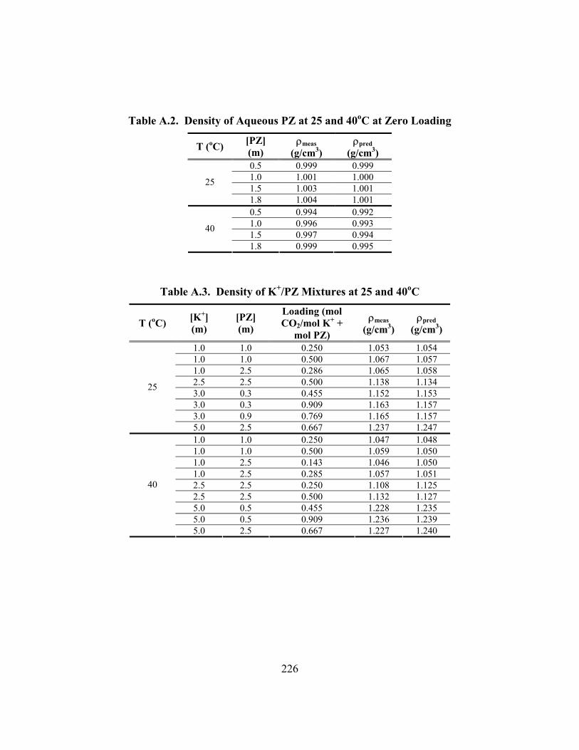
226
Table A.2. Density of Aqueous PZ at 25 and 40oC at Zero Loading
T (oC) [PZ] (m)
ρmeas (g/cm3)
ρpred (g/cm3)
0.5 0.999 0.999 1.0 1.001 1.000 1.5 1.003 1.001
25
1.8 1.004 1.001 0.5 0.994 0.992 1.0 0.996 0.993 1.5 0.997 0.994
40
1.8 0.999 0.995
Table A.3. Density of K+/PZ Mixtures at 25 and 40oC
T (oC) [K+] (m)
[PZ] (m)
Loading (mol CO2/mol K+ +
mol PZ)
ρmeas (g/cm3)
ρpred (g/cm3)
1.0 1.0 0.250 1.053 1.054 1.0 1.0 0.500 1.067 1.057 1.0 2.5 0.286 1.065 1.058 2.5 2.5 0.500 1.138 1.134 3.0 0.3 0.455 1.152 1.153 3.0 0.3 0.909 1.163 1.157 3.0 0.9 0.769 1.165 1.157
25
5.0 2.5 0.667 1.237 1.247 1.0 1.0 0.250 1.047 1.048 1.0 1.0 0.500 1.059 1.050 1.0 2.5 0.143 1.046 1.050 1.0 2.5 0.285 1.057 1.051 2.5 2.5 0.250 1.108 1.125 2.5 2.5 0.500 1.132 1.127 5.0 0.5 0.455 1.228 1.235 5.0 0.5 0.909 1.236 1.239
40
5.0 2.5 0.667 1.227 1.240
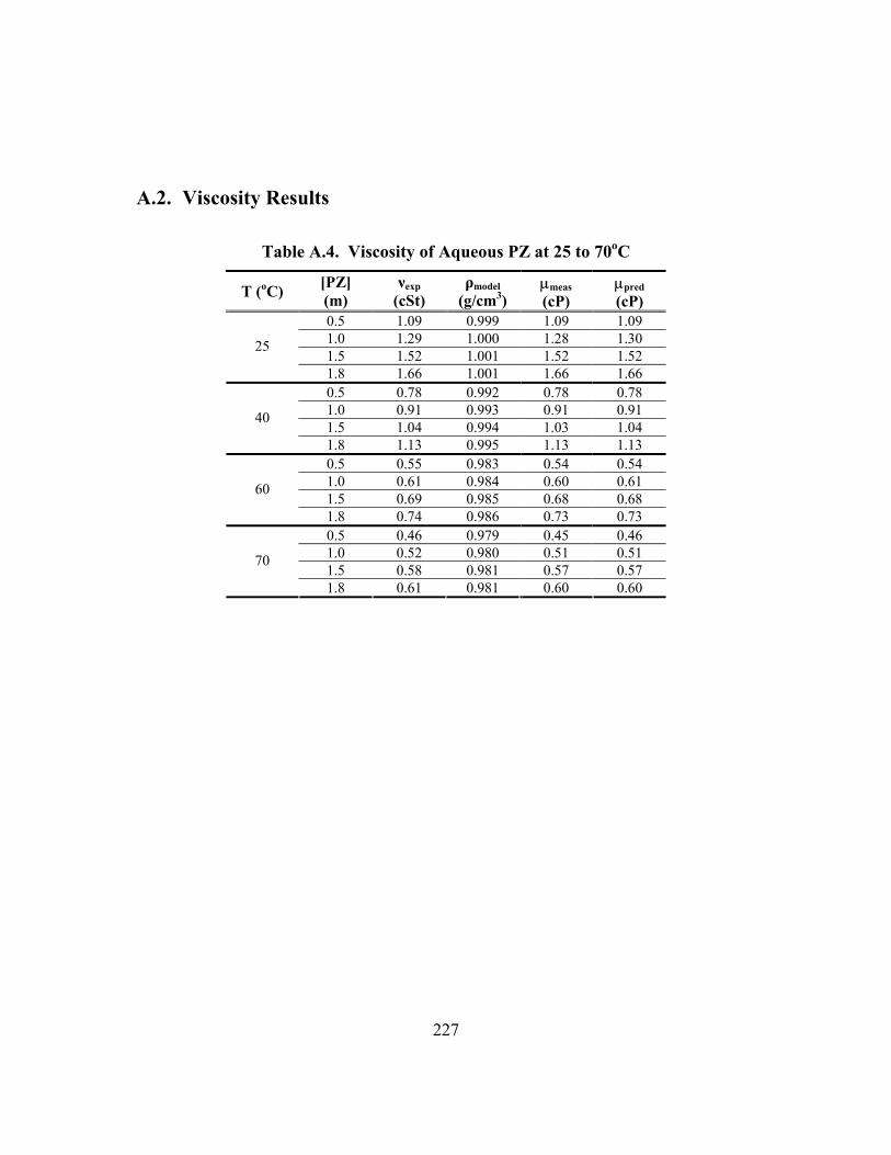
227
A.2. Viscosity Results
Table A.4. Viscosity of Aqueous PZ at 25 to 70oC
T (oC) [PZ] (m)
νexp (cSt)
ρmodel (g/cm3)
µmeas (cP)
µpred (cP)
0.5 1.09 0.999 1.09 1.09 1.0 1.29 1.000 1.28 1.30 1.5 1.52 1.001 1.52 1.52
25
1.8 1.66 1.001 1.66 1.66 0.5 0.78 0.992 0.78 0.78 1.0 0.91 0.993 0.91 0.91 1.5 1.04 0.994 1.03 1.04
40
1.8 1.13 0.995 1.13 1.13 0.5 0.55 0.983 0.54 0.54 1.0 0.61 0.984 0.60 0.61 1.5 0.69 0.985 0.68 0.68
60
1.8 0.74 0.986 0.73 0.73 0.5 0.46 0.979 0.45 0.46 1.0 0.52 0.980 0.51 0.51 1.5 0.58 0.981 0.57 0.57
70
1.8 0.61 0.981 0.60 0.60

228
Table A.5. Viscosity of K+/PZ Mixtures at 25 to 70oC
T (oC) [K+] (m)
[PZ] (m)
Loading (mol CO2/mol K+ +
mol PZ)
Νmeas (cSt) ρpred µmeas
(cP) µpred (cP)
3.0 0.0 1.000 1.14 1.157 1.32 1.39 5.0 0.0 0.500 1.53 1.241 1.90 1.91 0.5 1.0 0.167 1.35 1.028 1.39 1.40 0.5 1.0 0.334 1.35 1.029 1.39 1.39 1.0 2.0 0.333 2.00 1.057 2.11 2.03 1.0 1.0 0.250 1.40 1.054 1.48 1.50 1.0 1.0 0.500 1.40 1.057 1.48 1.50 1.0 2.0 0.167 2.02 1.056 2.13 2.04 2.0 1.0 0.333 1.58 1.105 1.74 1.74 2.0 1.0 0.667 1.53 1.108 1.70 1.73 2.0 2.0 0.500 2.17 1.109 2.40 2.36 3.6 3.6 0.500 4.13 1.187 4.90 4.71 4.0 2.0 0.667 2.59 1.203 3.12 3.21
25
5.0 2.5 0.667 3.33 1.247 4.15 4.35 1.0 1.0 0.250 1.01 1.048 1.06 1.05 1.0 2.0 0.167 1.35 1.049 1.42 1.38 1.0 2.0 0.333 1.35 1.050 1.41 1.38 2.0 1.0 0.333 1.12 1.099 1.23 1.22 2.0 1.0 0.667 1.11 1.102 1.22 1.22 2.0 2.0 0.500 1.48 1.102 1.64 1.60 3.0 1.0 0.375 1.25 1.147 1.43 1.42 3.6 3.6 0.500 2.64 1.180 3.12 3.01 4.0 2.0 0.667 1.79 1.196 2.14 2.17
40
5.0 2.5 0.667 2.23 1.240 2.77 2.88 0.5 1.0 0.167 0.65 1.012 0.66 0.66 0.5 1.0 0.334 0.64 1.014 0.65 0.66 1.0 1.0 0.250 0.68 1.039 0.71 0.71 1.0 1.0 0.500 0.68 1.041 0.71 0.71 1.0 2.0 0.167 0.87 1.040 0.90 0.89 1.0 2.0 0.333 0.87 1.042 0.91 0.88 2.0 1.0 0.333 0.76 1.090 0.83 0.83 2.0 1.0 0.667 0.75 1.093 0.82 0.82 2.0 2.0 0.500 0.96 1.093 1.05 1.03 3.6 3.6 0.500 1.60 1.171 1.87 1.81 4.0 2.0 0.667 1.16 1.188 1.38 1.39
60
5.0 2.5 0.667 1.42 1.231 1.75 1.80 1.0 1.0 0.250 0.57 1.034 0.59 0.60 1.0 2.0 0.167 0.70 1.036 0.73 0.73 1.0 2.0 0.333 0.72 1.037 0.74 0.73 2.0 1.0 0.333 0.64 1.085 0.69 0.70 2.0 1.0 0.667 0.63 1.088 0.69 0.69 2.0 2.0 0.500 0.79 1.089 0.87 0.85 3.0 1.0 0.375 0.71 1.133 0.80 0.81 3.6 3.6 0.500 1.27 1.167 1.49 1.45 4.0 2.0 0.667 0.96 1.183 1.13 1.15
70
5.0 2.5 0.667 1.16 1.227 1.42 1.47
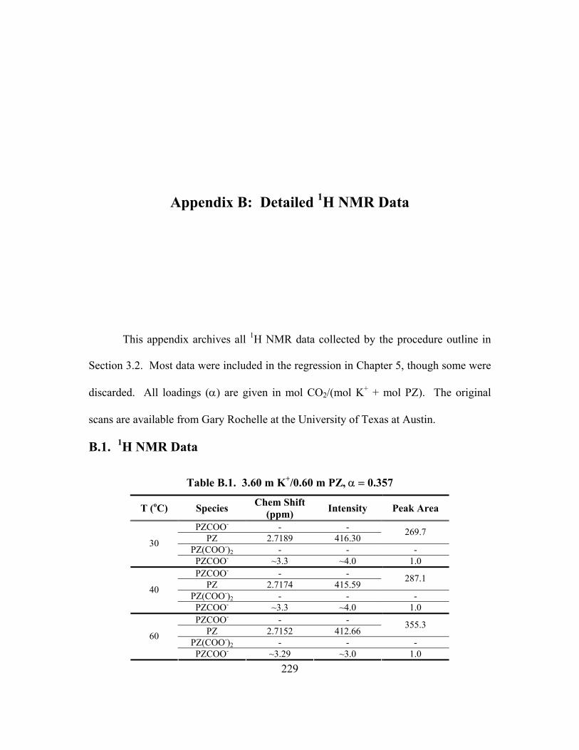
229
Appendix B: Detailed 1H NMR Data
This appendix archives all 1H NMR data collected by the procedure outline in
Section 3.2. Most data were included in the regression in Chapter 5, though some were
discarded. All loadings (α) are given in mol CO2/(mol K+ + mol PZ). The original
scans are available from Gary Rochelle at the University of Texas at Austin.
B.1. 1H NMR Data
Table B.1. 3.60 m K+/0.60 m PZ, α = 0.357
T (oC) Species Chem Shift (ppm) Intensity Peak Area
PZCOO- - - PZ 2.7189 416.30
269.7
PZ(COO-)2 - - - 30
PZCOO- ~3.3 ~4.0 1.0 PZCOO- - -
PZ 2.7174 415.59 287.1
PZ(COO-)2 - - - 40
PZCOO- ~3.3 ~4.0 1.0 PZCOO- - -
PZ 2.7152 412.66 355.3
PZ(COO-)2 - - - 60
PZCOO- ~3.29 ~3.0 1.0
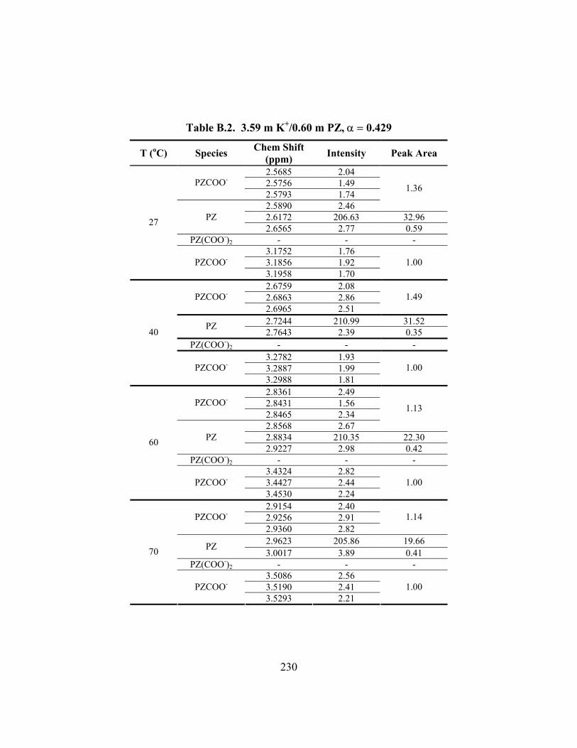
230
Table B.2. 3.59 m K+/0.60 m PZ, α = 0.429
T (oC) Species Chem Shift (ppm) Intensity Peak Area
2.5685 2.04 2.5756 1.49 PZCOO- 2.5793 1.74 2.5890 2.46
1.36
2.6172 206.63 32.96 PZ 2.6565 2.77 0.59
PZ(COO-)2 - - - 3.1752 1.76 3.1856 1.92
27
PZCOO- 3.1958 1.70
1.00
2.6759 2.08 2.6863 2.86 PZCOO- 2.6965 2.51
1.49
2.7244 210.99 31.52 PZ 2.7643 2.39 0.35
PZ(COO-)2 - - - 3.2782 1.93 3.2887 1.99
40
PZCOO- 3.2988 1.81
1.00
2.8361 2.49 2.8431 1.56 PZCOO- 2.8465 2.34 2.8568 2.67
1.13
2.8834 210.35 22.30 PZ 2.9227 2.98 0.42
PZ(COO-)2 - - - 3.4324 2.82 3.4427 2.44
60
PZCOO- 3.4530 2.24
1.00
2.9154 2.40 2.9256 2.91 PZCOO- 2.9360 2.82
1.14
2.9623 205.86 19.66 PZ 3.0017 3.89 0.41
PZ(COO-)2 - - - 3.5086 2.56 3.5190 2.41
70
PZCOO- 3.5293 2.21
1.00
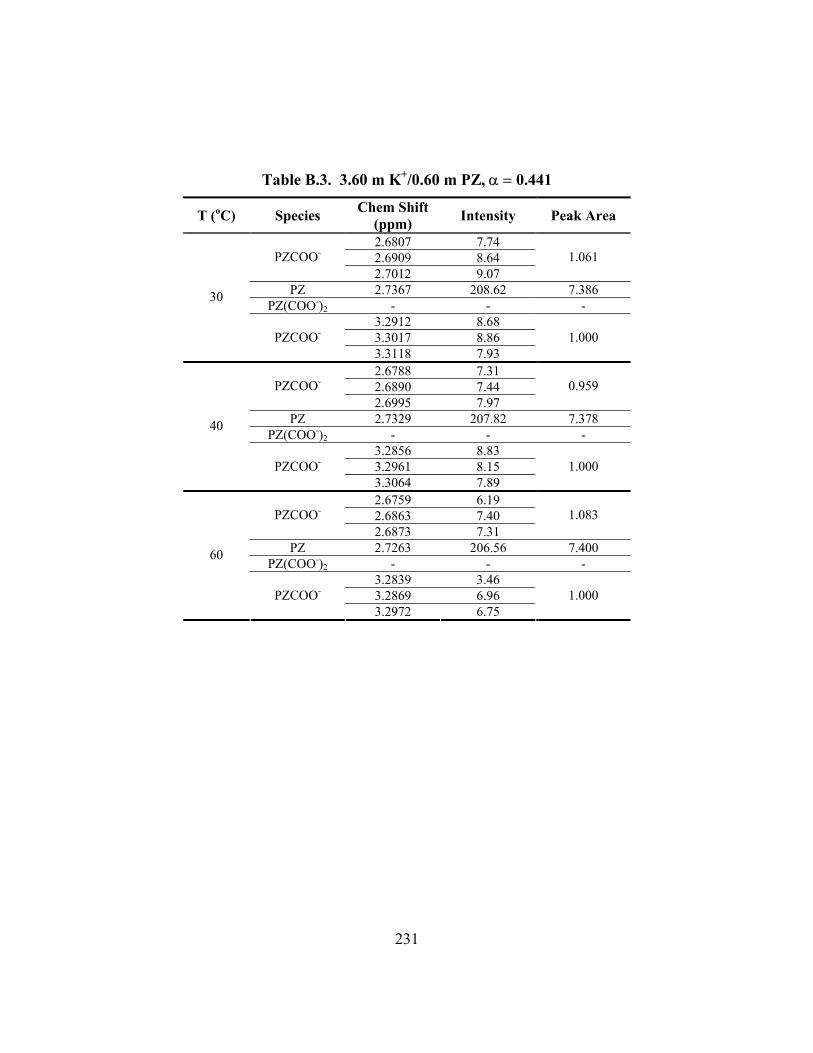
231
Table B.3. 3.60 m K+/0.60 m PZ, α = 0.441
T (oC) Species Chem Shift (ppm) Intensity Peak Area
2.6807 7.74 2.6909 8.64 PZCOO- 2.7012 9.07
1.061
PZ 2.7367 208.62 7.386 PZ(COO-)2 - - -
3.2912 8.68 3.3017 8.86
30
PZCOO- 3.3118 7.93
1.000
2.6788 7.31 2.6890 7.44 PZCOO- 2.6995 7.97
0.959
PZ 2.7329 207.82 7.378 PZ(COO-)2 - - -
3.2856 8.83 3.2961 8.15
40
PZCOO- 3.3064 7.89
1.000
2.6759 6.19 2.6863 7.40 PZCOO- 2.6873 7.31
1.083
PZ 2.7263 206.56 7.400 PZ(COO-)2 - - -
3.2839 3.46 3.2869 6.96
60
PZCOO- 3.2972 6.75
1.000
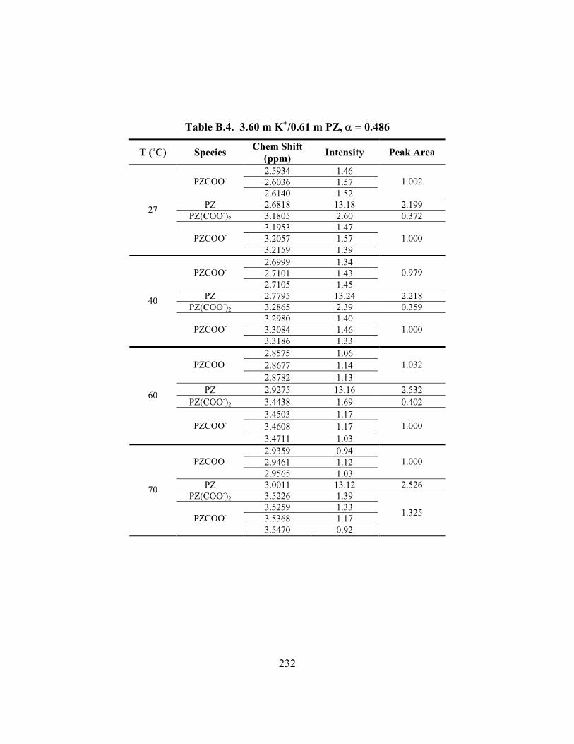
232
Table B.4. 3.60 m K+/0.61 m PZ, α = 0.486
T (oC) Species Chem Shift (ppm) Intensity Peak Area
2.5934 1.46 2.6036 1.57 PZCOO- 2.6140 1.52
1.002
PZ 2.6818 13.18 2.199 PZ(COO-)2 3.1805 2.60 0.372
3.1953 1.47 3.2057 1.57
27
PZCOO- 3.2159 1.39
1.000
2.6999 1.34 2.7101 1.43 PZCOO- 2.7105 1.45
0.979
PZ 2.7795 13.24 2.218 PZ(COO-)2 3.2865 2.39 0.359
3.2980 1.40 3.3084 1.46
40
PZCOO- 3.3186 1.33
1.000
2.8575 1.06 2.8677 1.14 PZCOO- 2.8782 1.13
1.032
PZ 2.9275 13.16 2.532 PZ(COO-)2 3.4438 1.69 0.402
3.4503 1.17 3.4608 1.17
60
PZCOO- 3.4711 1.03
1.000
2.9359 0.94 2.9461 1.12 PZCOO- 2.9565 1.03
1.000
PZ 3.0011 13.12 2.526 PZ(COO-)2 3.5226 1.39
3.5259 1.33 3.5368 1.17
70
PZCOO- 3.5470 0.92
1.325

233
Table B.5. 3.59 m K+/0.61 m PZ, α = 0.515
T (oC) Species Chem Shift (ppm) Intensity Peak Area
2.6200 2.34 2.6301 2.58 PZCOO- 2.6406 2.48
0.992
PZ 2.7374 13.00 1.278 PZ(COO-)2 3.1859 7.80 0.752
3.2155 2.42 3.2259 2.62
27
PZCOO- 3.2361 2.23
1.000
2.7236 2.21 2.7338 2.42 PZCOO- 2.7443 2.34
0.994
PZ 2.8293 13.09 1.328 PZ(COO-)2 3.2932 6.89 0.698
3.3166 2.30 3.3270 2.47
40
PZCOO- 3.3373 2.15
1.000
2.8760 1.95 2.8862 2.37 PZCOO- 2.8966 2.08
0.960
PZ 2.9644 13.03 1.409 PZ(COO-)2 3.4507 4.74 0.595
3.4654 2.21 3.4759 2.45
60
PZCOO- 3.4860 1.94
1.000
2.9527 2.06 2.9625 2.84 PZCOO- 2.9728 2.28
1.000
PZ 3.0326 12.98 1.525 PZ(COO-)2 3.5300 4.01
3.5397 2.92 3.5501 3.01
70
PZCOO- 3.5604 2.06
1.532
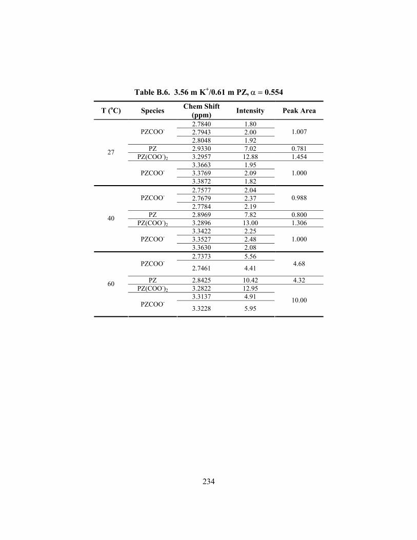
234
Table B.6. 3.56 m K+/0.61 m PZ, α = 0.554
T (oC) Species Chem Shift (ppm) Intensity Peak Area
2.7840 1.80 2.7943 2.00 PZCOO- 2.8048 1.92
1.007
PZ 2.9330 7.02 0.781 PZ(COO-)2 3.2957 12.88 1.454
3.3663 1.95 3.3769 2.09
27
PZCOO- 3.3872 1.82
1.000
2.7577 2.04 2.7679 2.37 PZCOO- 2.7784 2.19
0.988
PZ 2.8969 7.82 0.800 PZ(COO-)2 3.2896 13.00 1.306
3.3422 2.25 3.3527 2.48
40
PZCOO- 3.3630 2.08
1.000
2.7373 5.56 PZCOO-
2.7461 4.41 4.68
PZ 2.8425 10.42 4.32 PZ(COO-)2 3.2822 12.95
3.3137 4.91
60
PZCOO- 3.3228 5.95 10.00
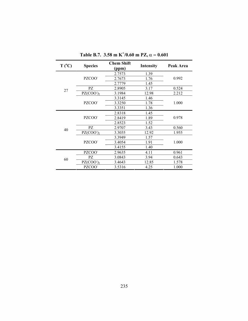
235
Table B.7. 3.58 m K+/0.60 m PZ, α = 0.601
T (oC) Species Chem Shift (ppm) Intensity Peak Area
2.7573 1.39 2.7673 1.76 PZCOO- 2.7779 1.45
0.992
PZ 2.8905 3.17 0.524 PZ(COO-)2 3.1984 12.98 2.212
3.3145 1.46 3.3250 1.78
27
PZCOO- 3.3351 1.36
1.000
2.8318 1.45 2.8419 1.89 PZCOO- 2.8523 1.52
0.978
PZ 2.9707 3.43 0.560 PZ(COO-)2 3.3035 12.92 1.955
3.3949 1.57 3.4054 1.91
40
PZCOO- 3.4155 1.40
1.000
PZCOO- 2.9635 4.11 0.961 PZ 3.0843 3.94 0.643
PZ(COO-)2 3.4643 12.85 1.578 60
PZCOO- 3.5316 4.25 1.000

236
Table B.8. 3.59 m K+/0.61 m PZ, α = 0.630
T (oC) Species Chem Shift (ppm) Intensity Peak Area
2.7986 1.16 2.8088 1.50 PZCOO- 2.8193 1.24
0.987
PZ 2.9131 2.32 0.431 PZ(COO-)2 3.1978 13.06 2.517
3.3426 1.25 3.3531 1.52
27
PZCOO- 3.3633 1.15
1.000
2.8687 1.28 2.8788 1.79 PZCOO- 2.8889 1.38
0.992
PZ 2.9982 2.40 0.501 PZ(COO-)2 3.3046 13.13 2.328
3.4205 1.43 3.4307 1.81
40
PZCOO- 3.4408 1.26
1.00
PZCOO- 2.9912 3.82 0.928 PZ 3.1134 2.75 0.567
PZ(COO-)2 3.4662 12.88 1.907 60
PZCOO- 3.5496 4.08 1.000
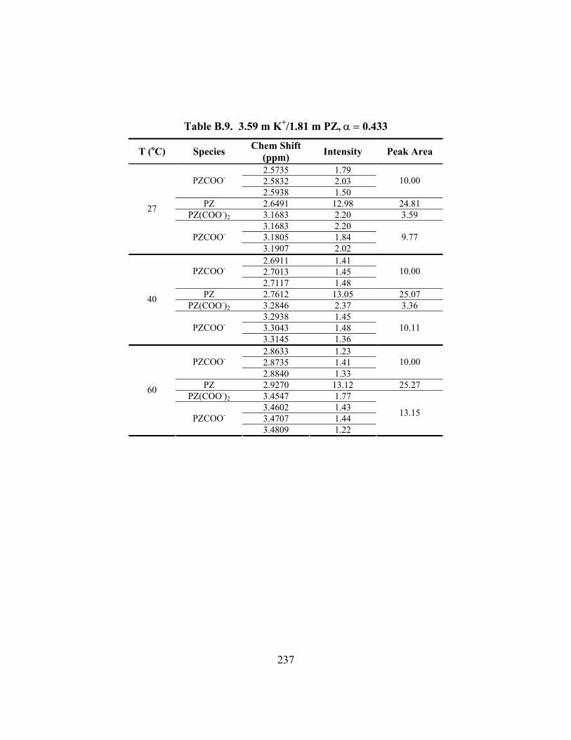
237
Table B.9. 3.59 m K+/1.81 m PZ, α = 0.433
T (oC) Species Chem Shift (ppm) Intensity Peak Area
2.5735 1.79 2.5832 2.03 PZCOO- 2.5938 1.50
10.00
PZ 2.6491 12.98 24.81 PZ(COO-)2 3.1683 2.20 3.59
3.1683 2.20 3.1805 1.84
27
PZCOO- 3.1907 2.02
9.77
2.6911 1.41 2.7013 1.45 PZCOO- 2.7117 1.48
10.00
PZ 2.7612 13.05 25.07 PZ(COO-)2 3.2846 2.37 3.36
3.2938 1.45 3.3043 1.48
40
PZCOO- 3.3145 1.36
10.11
2.8633 1.23 2.8735 1.41 PZCOO- 2.8840 1.33
10.00
PZ 2.9270 13.12 25.27 PZ(COO-)2 3.4547 1.77
3.4602 1.43 3.4707 1.44
60
PZCOO- 3.4809 1.22
13.15
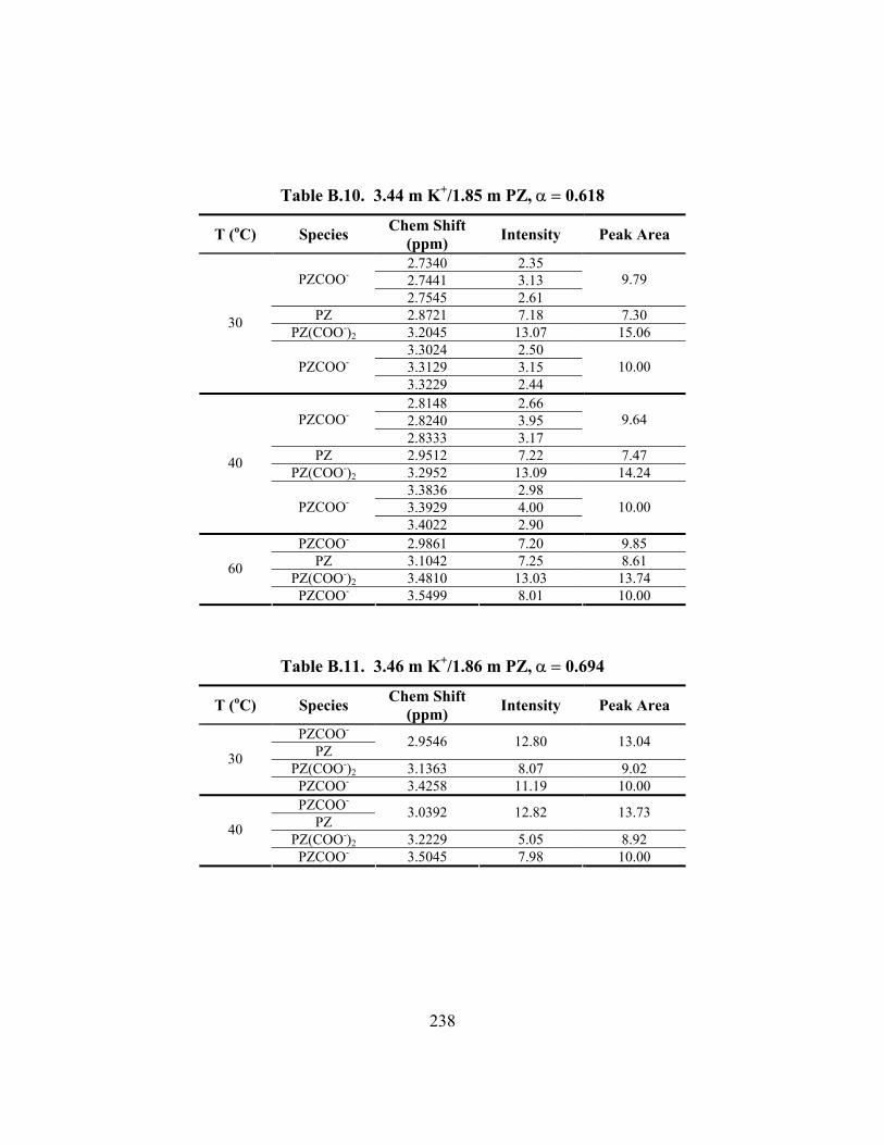
238
Table B.10. 3.44 m K+/1.85 m PZ, α = 0.618
T (oC) Species Chem Shift (ppm) Intensity Peak Area
2.7340 2.35 2.7441 3.13 PZCOO- 2.7545 2.61
9.79
PZ 2.8721 7.18 7.30 PZ(COO-)2 3.2045 13.07 15.06
3.3024 2.50 3.3129 3.15
30
PZCOO- 3.3229 2.44
10.00
2.8148 2.66 2.8240 3.95 PZCOO- 2.8333 3.17
9.64
PZ 2.9512 7.22 7.47 PZ(COO-)2 3.2952 13.09 14.24
3.3836 2.98 3.3929 4.00
40
PZCOO- 3.4022 2.90
10.00
PZCOO- 2.9861 7.20 9.85 PZ 3.1042 7.25 8.61
PZ(COO-)2 3.4810 13.03 13.74 60
PZCOO- 3.5499 8.01 10.00
Table B.11. 3.46 m K+/1.86 m PZ, α = 0.694
T (oC) Species Chem Shift (ppm) Intensity Peak Area
PZCOO- PZ
2.9546 12.80 13.04
PZ(COO-)2 3.1363 8.07 9.02 30
PZCOO- 3.4258 11.19 10.00 PZCOO-
PZ 3.0392 12.82 13.73
PZ(COO-)2 3.2229 5.05 8.92 40
PZCOO- 3.5045 7.98 10.00

239
Table B.12. 3.60 m K+/3.58 m PZ, α = 0.376
T (oC) Species Chem Shift (ppm) Intensity Peak Area
2.6914 1.56 2.7017 1.71 PZCOO- 2.7121 1.66
10.00
PZ 2.7532 13.03 32.20 PZ(COO-)2 3.2913 1.84 2.30
3.3000 1.60 3.3104 1.73
40
PZCOO- 3.3206 1.53
9.87
2.8774 1.34 2.8876 1.55 PZCOO- 2.8980 1.48
10.00
PZ 2.9361 13.18 32.52 PZ(COO-)2 3.4743 1.43
3.4798 1.50 3.4903 1.57
60
PZCOO- 3.5005 1.32
12.15
Table B.13. 3.57 m K+/3.58 m PZ, α = 0.499
T (oC) Species Chem Shift (ppm) Intensity Peak Area
2.5837 2.65 2.5939 2.92 PZCOO- 2.6044 2.66
10.00
PZ 2.6946 12.92 14.57 PZ(COO-)2 3.1575 6.60 6.43
3.1874 2.69 3.1978 2.95
27
PZCOO- 3.2080 2.49
10.17
2.7126 2.55 2.7229 2.91 PZCOO- 2.7333 2.59
10.00
PZ 2.8177 13.10 14.65 PZ(COO-)2 3.2850 6.04 6.57
3.3122 2.66 3.3226 2.99
40
PZCOO- 3.3328 2.44
10.24
PZCOO- 2.9064 4.28 10.00 PZ 2.9923 12.86 14.78
PZ(COO-)2 3.4670 4.67 60
PZCOO- 3.4991 4.58 16.33
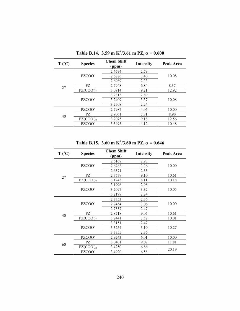
240
Table B.14. 3.59 m K+/3.61 m PZ, α = 0.600
T (oC) Species Chem Shift (ppm) Intensity Peak Area
2.6794 2.79 2.6886 3.40 PZCOO- 2.6989 2.33
10.08
PZ 2.7948 6.84 8.37 PZ(COO-)2 3.0914 9.21 12.92
3.2313 2.89 3.2409 3.37
27
PZCOO- 3.2508 2.24
10.08
PZCOO- 2.7987 4.06 10.00 PZ 2.9061 7.81 8.90
PZ(COO-)2 3.2075 9.18 12.56 40
PZCOO- 3.3495 4.12 10.48
Table B.15. 3.60 m K+/3.60 m PZ, α = 0.646
T (oC) Species Chem Shift (ppm) Intensity Peak Area
2.6168 2.93 2.6263 3.36 PZCOO- 2.6371 2.33
10.00
PZ 2.7579 9.10 10.61 PZ(COO-)2 3.1243 8.11 10.18
3.1996 2.98 3.2097 3.32
27
PZCOO- 3.2198 2.24
10.05
2.7353 2.36 2.7454 3.06 PZCOO- 2.7557 2.47
10.00
PZ 2.8718 9.05 10.61 PZ(COO-)2 3.2441 7.52 10.01
3.3151 2.47 3.3254 3.10
40
PZCOO- 3.3355 2.36
10.27
PZCOO- 2.9243 6.01 10.00 PZ 3.0401 9.07 11.81
PZ(COO-)2 3.4250 6.86 60
PZCOO- 3.4920 6.58 20.19

241
Table B.16. 5.00 m K+/2.50 m PZ, α = 0.433
T (oC) Species Chem Shift (ppm) Intensity Peak Area
2.4226 4.35 2.4328 8.40 PZCOO- 2.4428 4.68
11.71
PZ 2.5290 128.63 76.31 PZ(COO-)2 2.9939 3.00 1.49
3.0251 4.55 3.0351 8.20
30
PZCOO- 3.0451 4.24
10.50
2.4232 6.58 2.4331 12.66 PZCOO- 2.4429 7.84
14.29
PZ 2.5157 149.53 69.47 PZ(COO-)2 3.0022 5.79 2.62
3.0249 6.62 3.0348 12.52
40
PZCOO- 3.0446 6.94
13.62
2.4289 10.14 2.4391 17.26 PZCOO- 2.4492 9.91
20.28
PZ 2.4881 120.13 53.55 PZ(COO-)2 3.0243 15.52
3.0296 10.56 3.0398 17.00
60
PZCOO- 3.0499 9.04
26.17
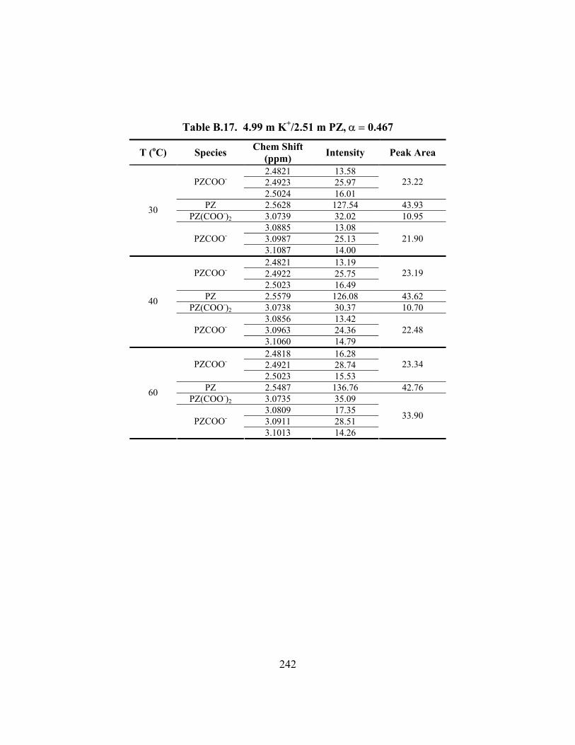
242
Table B.17. 4.99 m K+/2.51 m PZ, α = 0.467
T (oC) Species Chem Shift (ppm) Intensity Peak Area
2.4821 13.58 2.4923 25.97 PZCOO- 2.5024 16.01
23.22
PZ 2.5628 127.54 43.93 PZ(COO-)2 3.0739 32.02 10.95
3.0885 13.08 3.0987 25.13
30
PZCOO- 3.1087 14.00
21.90
2.4821 13.19 2.4922 25.75 PZCOO- 2.5023 16.49
23.19
PZ 2.5579 126.08 43.62 PZ(COO-)2 3.0738 30.37 10.70
3.0856 13.42 3.0963 24.36
40
PZCOO- 3.1060 14.79
22.48
2.4818 16.28 2.4921 28.74 PZCOO- 2.5023 15.53
23.34
PZ 2.5487 136.76 42.76 PZ(COO-)2 3.0735 35.09
3.0809 17.35 3.0911 28.51
60
PZCOO- 3.1013 14.26
33.90

243
Table B.18. 4.98 m K+/2.50 m PZ, α = 0.534
T (oC) Species Chem Shift (ppm) Intensity Peak Area
2.5137 21.68 2.5240 37.22 PZCOO- 2.5342 23.55
25.44
PZ 2.6314 126.98 27.93 PZ(COO-)2 3.0769 95.72 21.97
3.1111 23.40 3.1213 36.72
30
PZCOO- 3.1314 21.49
24.66
2.5138 24.47 2.5240 46.42 PZCOO- 2.5341 28.49
25.65
PZ 2.6234 145.13 27.22 PZ(COO-)2 3.0807 109.50 22.50
3.1098 26.82 3.1198 46.08
40
PZCOO- 3.1298 26.58
24.63
PZCOO- 2.5236 62.34 25.44 PZ 2.6069 124.83 26.53
PZ(COO-)2 3.0862 95.69 23.03 60
PZCOO- 3.1151 61.45 25.00
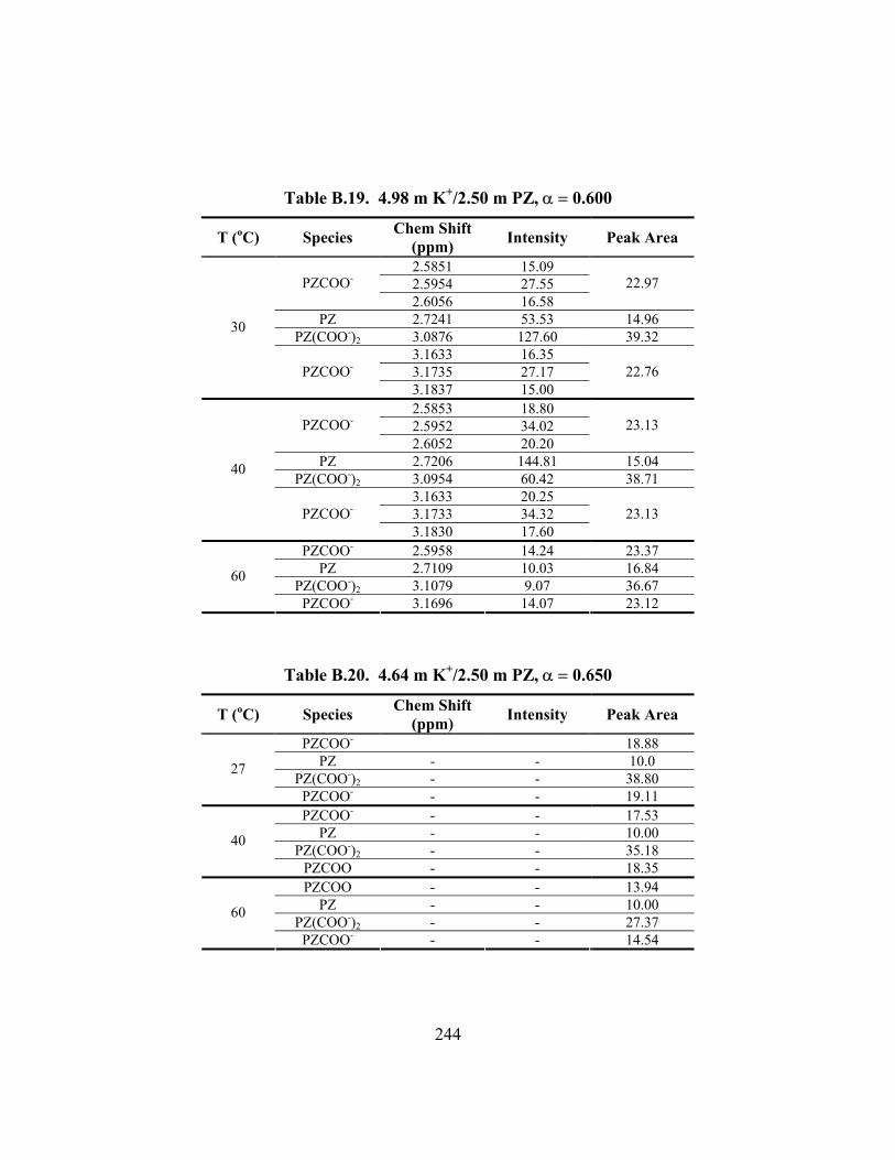
244
Table B.19. 4.98 m K+/2.50 m PZ, α = 0.600
T (oC) Species Chem Shift (ppm) Intensity Peak Area
2.5851 15.09 2.5954 27.55 PZCOO- 2.6056 16.58
22.97
PZ 2.7241 53.53 14.96 PZ(COO-)2 3.0876 127.60 39.32
3.1633 16.35 3.1735 27.17
30
PZCOO- 3.1837 15.00
22.76
2.5853 18.80 2.5952 34.02 PZCOO- 2.6052 20.20
23.13
PZ 2.7206 144.81 15.04 PZ(COO-)2 3.0954 60.42 38.71
3.1633 20.25 3.1733 34.32
40
PZCOO- 3.1830 17.60
23.13
PZCOO- 2.5958 14.24 23.37 PZ 2.7109 10.03 16.84
PZ(COO-)2 3.1079 9.07 36.67 60
PZCOO- 3.1696 14.07 23.12
Table B.20. 4.64 m K+/2.50 m PZ, α = 0.650
T (oC) Species Chem Shift (ppm) Intensity Peak Area
PZCOO- 18.88 PZ - - 10.0
PZ(COO-)2 - - 38.80 27
PZCOO- - - 19.11 PZCOO- - - 17.53
PZ - - 10.00 PZ(COO-)2 - - 35.18
40
PZCOO - - 18.35 PZCOO - - 13.94
PZ - - 10.00 PZ(COO-)2 - - 27.37
60
PZCOO- - - 14.54

245
Table B.21. 6.18 m K+/1.23 m PZ, α = 0.570
T (oC) Species Chem Shift (ppm) Intensity Peak Area
2.7870 1.83 2.7972 2.21 PZCOO- 2.8077 1.91
9.82
PZ 2.9324 5.95 6.82 PZ(COO-)2 3.2865 13.00 16.06
3.3658 2.01 3.3764 2.28
27
PZCOO- 3.3866 1.83
10.00
2.7504 1.74 2.7606 2.15 PZCOO- 2.7710 1.79
9.62
PZ 2.8868 4.26 5.65 PZ(COO-)2 3.2812 13.00 17.67
3.3344 1.89 3.3448 2.21
40
PZCOO- 3.3550 1.70
10.00
PZCOO- 2.7279 3.55 9.52 PZ 2.8315 3.80 5.96
PZ(COO-)2 3.2727 13.09 15.50 3.3043 3.33
60
PZCOO- 3.3123 3.80 10.00
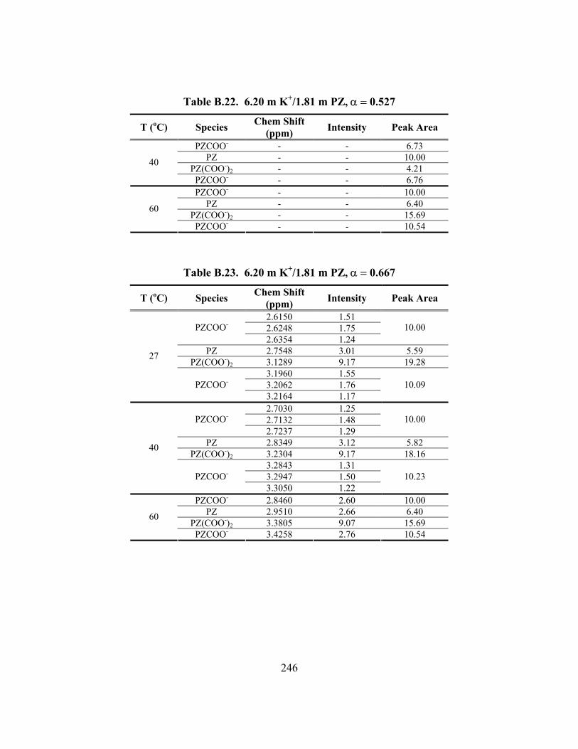
246
Table B.22. 6.20 m K+/1.81 m PZ, α = 0.527
T (oC) Species Chem Shift (ppm) Intensity Peak Area
PZCOO- - - 6.73 PZ - - 10.00
PZ(COO-)2 - - 4.21 40
PZCOO- - - 6.76 PZCOO- - - 10.00
PZ - - 6.40 PZ(COO-)2 - - 15.69
60
PZCOO- - - 10.54
Table B.23. 6.20 m K+/1.81 m PZ, α = 0.667
T (oC) Species Chem Shift (ppm) Intensity Peak Area
2.6150 1.51 2.6248 1.75 PZCOO- 2.6354 1.24
10.00
PZ 2.7548 3.01 5.59 PZ(COO-)2 3.1289 9.17 19.28
3.1960 1.55 3.2062 1.76
27
PZCOO- 3.2164 1.17
10.09
2.7030 1.25 2.7132 1.48 PZCOO- 2.7237 1.29
10.00
PZ 2.8349 3.12 5.82 PZ(COO-)2 3.2304 9.17 18.16
3.2843 1.31 3.2947 1.50
40
PZCOO- 3.3050 1.22
10.23
PZCOO- 2.8460 2.60 10.00 PZ 2.9510 2.66 6.40
PZ(COO-)2 3.3805 9.07 15.69 60
PZCOO- 3.4258 2.76 10.54
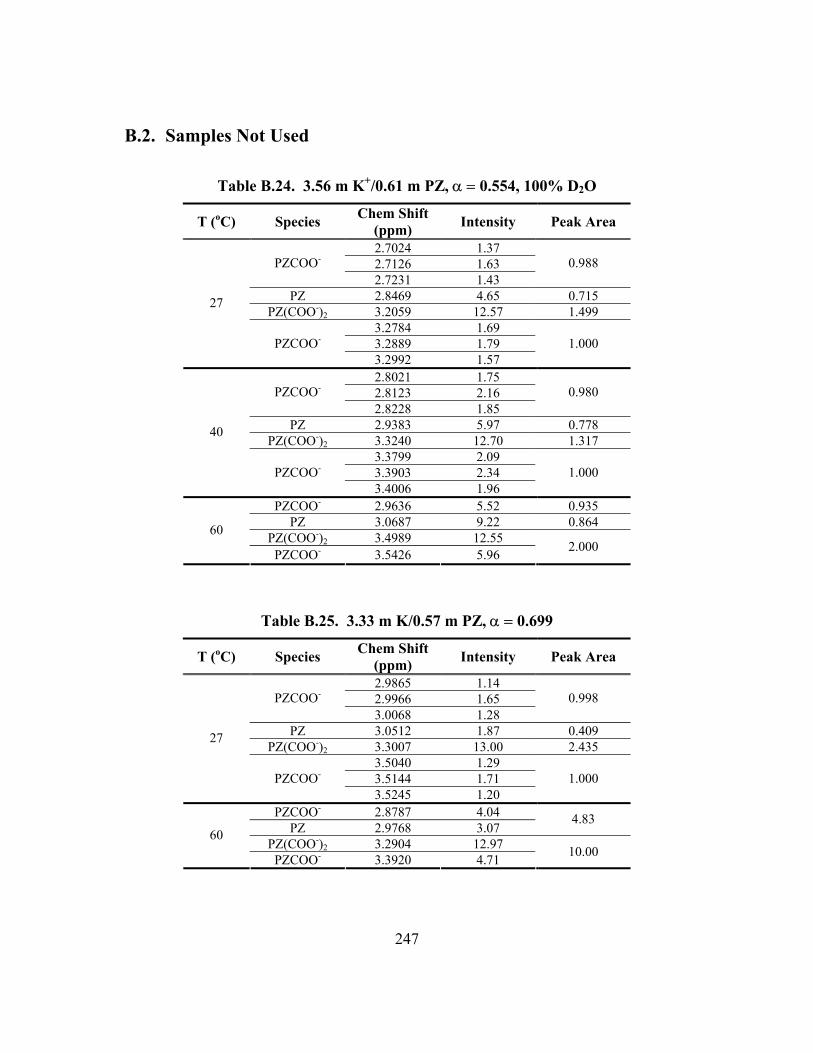
247
B.2. Samples Not Used
Table B.24. 3.56 m K+/0.61 m PZ, α = 0.554, 100% D2O
T (oC) Species Chem Shift (ppm) Intensity Peak Area
2.7024 1.37 2.7126 1.63 PZCOO- 2.7231 1.43
0.988
PZ 2.8469 4.65 0.715 PZ(COO-)2 3.2059 12.57 1.499
3.2784 1.69 3.2889 1.79
27
PZCOO- 3.2992 1.57
1.000
2.8021 1.75 2.8123 2.16 PZCOO- 2.8228 1.85
0.980
PZ 2.9383 5.97 0.778 PZ(COO-)2 3.3240 12.70 1.317
3.3799 2.09 3.3903 2.34
40
PZCOO- 3.4006 1.96
1.000
PZCOO- 2.9636 5.52 0.935 PZ 3.0687 9.22 0.864
PZ(COO-)2 3.4989 12.55 60
PZCOO- 3.5426 5.96 2.000
Table B.25. 3.33 m K/0.57 m PZ, α = 0.699
T (oC) Species Chem Shift (ppm) Intensity Peak Area
2.9865 1.14 2.9966 1.65 PZCOO- 3.0068 1.28
0.998
PZ 3.0512 1.87 0.409 PZ(COO-)2 3.3007 13.00 2.435
3.5040 1.29 3.5144 1.71
27
PZCOO- 3.5245 1.20
1.000
PZCOO- 2.8787 4.04 PZ 2.9768 3.07
4.83
PZ(COO-)2 3.2904 12.97 60
PZCOO- 3.3920 4.71 10.00
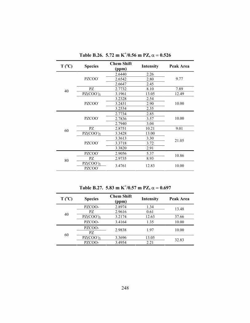
248
Table B.26. 5.72 m K+/0.56 m PZ, α = 0.526
T (oC) Species Chem Shift (ppm) Intensity Peak Area
2.6440 2.26 2.6542 2.80 PZCOO- 2.6647 2.45
9.77
PZ 2.7732 8.10 7.89 PZ(COO-)2 3.1961 13.05 12.49
3.2328 2.54 3.2431 2.90
40
PZCOO- 3.2534 2.35
10.00
2.7734 2.85 2.7836 3.57 PZCOO- 2.7940 3.04
10.00
PZ 2.8751 10.21 9.01 PZ(COO-)2 3.3428 13.00
3.3613 3.30 3.3718 3.72
60
PZCOO- 3.3820 2.91
21.05
PZCOO- 2.9056 5.37 PZ 2.9735 8.93
10.86
PZ(COO-)2 80
PZCOO- 3.4761 12.83 10.00
Table B.27. 5.83 m K+/0.57 m PZ, α = 0.697
T (oC) Species Chem Shift (ppm) Intensity Peak Area
PZCOO- 2.8974 1.34 PZ 2.9616 0.61
13.48
PZ(COO-)2 3.2174 12.63 37.66 40
PZCOO- 3.4164 1.35 10.00 PZCOO-
PZ 2.9838 1.97 10.00
PZ(COO-)2 3.3696 13.05 60
PZCOO- 3.4954 2.21 32.83

249
B.3. Example Spectra
Figure B.1. 1H NMR Spectrum of 3.6 m K+/0.6 m PZ, a = 0.600, T = 27oC
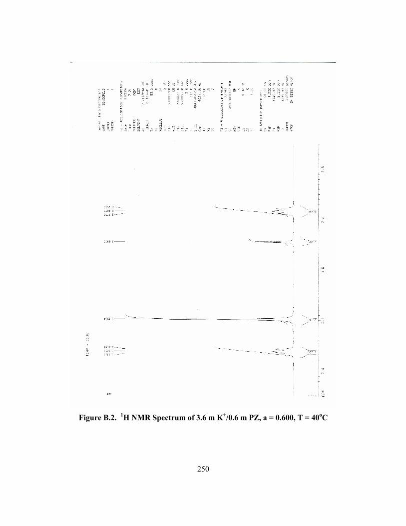
250
Figure B.2. 1H NMR Spectrum of 3.6 m K+/0.6 m PZ, a = 0.600, T = 40oC
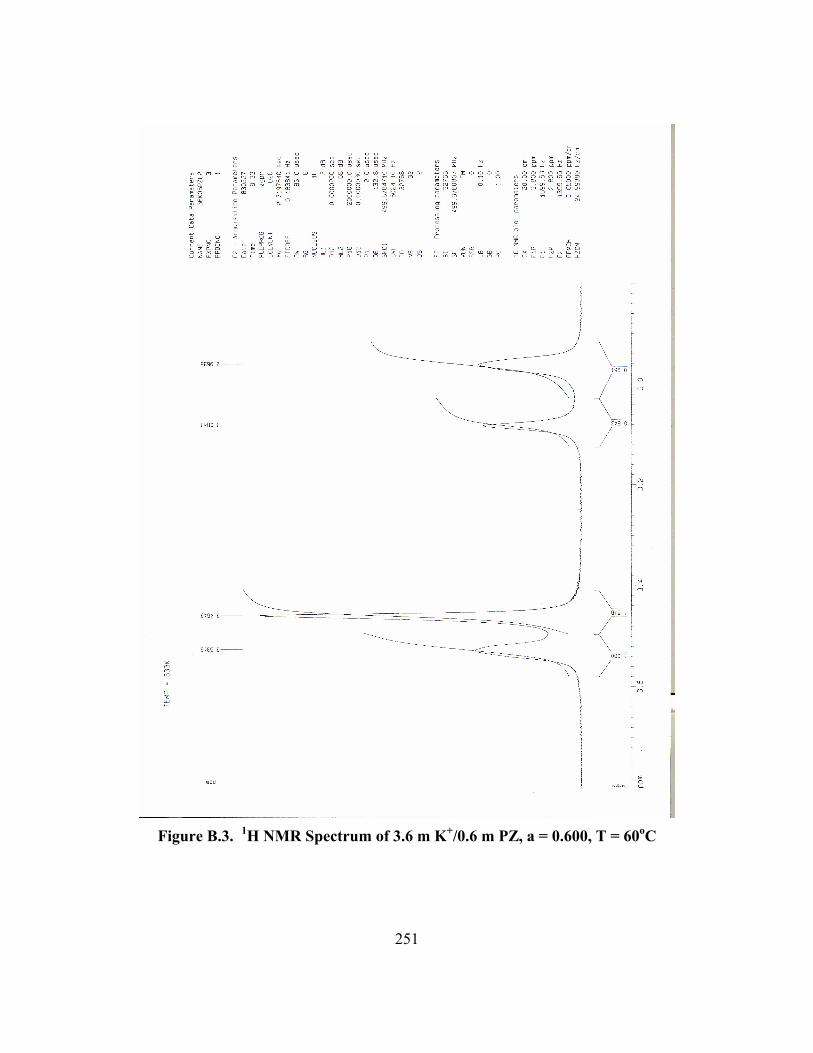
251
Figure B.3. 1H NMR Spectrum of 3.6 m K+/0.6 m PZ, a = 0.600, T = 60oC
252
Appendix C: Detailed Wetted-Wall Column Data
This appendix presents the detailed results of the wetted-wall column
experiments used to calculate the equilibrium partial pressure and the absorption rate of
CO2 in K+/PZ mixtures. An asterisk indicates points that were used for modeling the
absorption rate; these points typically have a moderate driving force and CO2 removal.
The temperature is an average of the inlet and outlet liquid temperatures; ∆T across the
column was typically no more than 1 to 3oC. A predicted loading is also presented,
indicating the loading required for the ENRTL model to match the measured PCO2*
exactly. The predicted flux is based on rigorous rate model calculations with the
predicted loading, relying on the measured partial pressure driving force to eliminate
errors associated with loading and thermodynamic estimates.
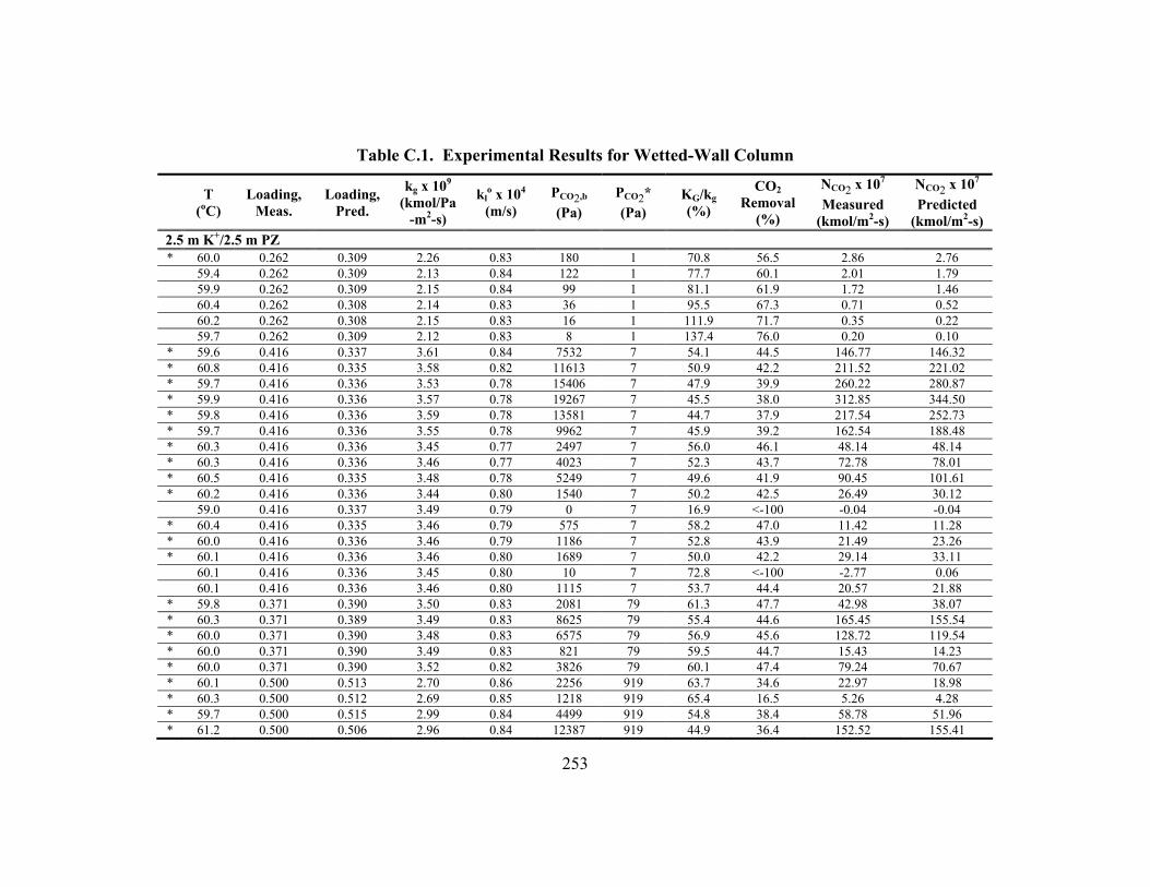
253
Table C.1. Experimental Results for Wetted-Wall Column
T (oC)
Loading, Meas.
Loading, Pred.
kg x 109 (kmol/Pa
-m2-s)
klo x 104 (m/s)
PCO2,b (Pa)
PCO2* (Pa)
KG/kg (%)
CO2 Removal
(%)
NCO2 x 107 Measured
(kmol/m2-s)
NCO2 x 107 Predicted
(kmol/m2-s) 2.5 m K+/2.5 m PZ * 60.0 0.262 0.309 2.26 0.83 180 1 70.8 56.5 2.86 2.76 59.4 0.262 0.309 2.13 0.84 122 1 77.7 60.1 2.01 1.79 59.9 0.262 0.309 2.15 0.84 99 1 81.1 61.9 1.72 1.46 60.4 0.262 0.308 2.14 0.83 36 1 95.5 67.3 0.71 0.52 60.2 0.262 0.308 2.15 0.83 16 1 111.9 71.7 0.35 0.22 59.7 0.262 0.309 2.12 0.83 8 1 137.4 76.0 0.20 0.10 * 59.6 0.416 0.337 3.61 0.84 7532 7 54.1 44.5 146.77 146.32 * 60.8 0.416 0.335 3.58 0.82 11613 7 50.9 42.2 211.52 221.02 * 59.7 0.416 0.336 3.53 0.78 15406 7 47.9 39.9 260.22 280.87 * 59.9 0.416 0.336 3.57 0.78 19267 7 45.5 38.0 312.85 344.50 * 59.8 0.416 0.336 3.59 0.78 13581 7 44.7 37.9 217.54 252.73 * 59.7 0.416 0.336 3.55 0.78 9962 7 45.9 39.2 162.54 188.48 * 60.3 0.416 0.336 3.45 0.77 2497 7 56.0 46.1 48.14 48.14 * 60.3 0.416 0.336 3.46 0.77 4023 7 52.3 43.7 72.78 78.01 * 60.5 0.416 0.335 3.48 0.78 5249 7 49.6 41.9 90.45 101.61 * 60.2 0.416 0.336 3.44 0.80 1540 7 50.2 42.5 26.49 30.12 59.0 0.416 0.337 3.49 0.79 0 7 16.9 <-100 -0.04 -0.04 * 60.4 0.416 0.335 3.46 0.79 575 7 58.2 47.0 11.42 11.28 * 60.0 0.416 0.336 3.46 0.79 1186 7 52.8 43.9 21.49 23.26 * 60.1 0.416 0.336 3.46 0.80 1689 7 50.0 42.2 29.14 33.11 60.1 0.416 0.336 3.45 0.80 10 7 72.8 <-100 -2.77 0.06 60.1 0.416 0.336 3.46 0.80 1115 7 53.7 44.4 20.57 21.88 * 59.8 0.371 0.390 3.50 0.83 2081 79 61.3 47.7 42.98 38.07 * 60.3 0.371 0.389 3.49 0.83 8625 79 55.4 44.6 165.45 155.54 * 60.0 0.371 0.390 3.48 0.83 6575 79 56.9 45.6 128.72 119.54 * 60.0 0.371 0.390 3.49 0.83 821 79 59.5 44.7 15.43 14.23 * 60.0 0.371 0.390 3.52 0.82 3826 79 60.1 47.4 79.24 70.67 * 60.1 0.500 0.513 2.70 0.86 2256 919 63.7 34.6 22.97 18.98 * 60.3 0.500 0.512 2.69 0.85 1218 919 65.4 16.5 5.26 4.28 * 59.7 0.500 0.515 2.99 0.84 4499 919 54.8 38.4 58.78 51.96 * 61.2 0.500 0.506 2.96 0.84 12387 919 44.9 36.4 152.52 155.41
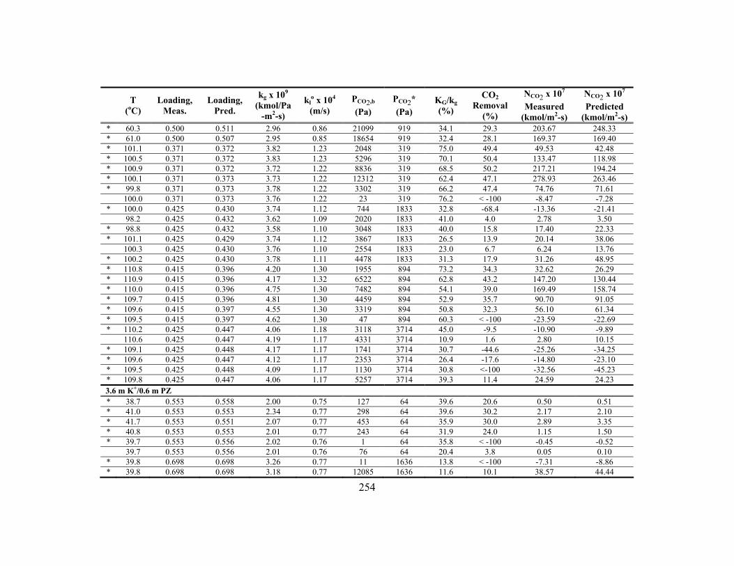
254
T (oC)
Loading, Meas.
Loading, Pred.
kg x 109 (kmol/Pa
-m2-s)
klo x 104 (m/s)
PCO2,b (Pa)
PCO2* (Pa)
KG/kg (%)
CO2 Removal
(%)
NCO2 x 107 Measured
(kmol/m2-s)
NCO2 x 107 Predicted
(kmol/m2-s) * 60.3 0.500 0.511 2.96 0.86 21099 919 34.1 29.3 203.67 248.33 * 61.0 0.500 0.507 2.95 0.85 18654 919 32.4 28.1 169.37 169.40 * 101.1 0.371 0.372 3.82 1.23 2048 319 75.0 49.4 49.53 42.48 * 100.5 0.371 0.372 3.83 1.23 5296 319 70.1 50.4 133.47 118.98 * 100.9 0.371 0.372 3.72 1.22 8836 319 68.5 50.2 217.21 194.24 * 100.1 0.371 0.373 3.73 1.22 12312 319 62.4 47.1 278.93 263.46 * 99.8 0.371 0.373 3.78 1.22 3302 319 66.2 47.4 74.76 71.61 100.0 0.371 0.373 3.76 1.22 23 319 76.2 < -100 -8.47 -7.28 * 100.0 0.425 0.430 3.74 1.12 744 1833 32.8 -68.4 -13.36 -21.41 98.2 0.425 0.432 3.62 1.09 2020 1833 41.0 4.0 2.78 3.50 * 98.8 0.425 0.432 3.58 1.10 3048 1833 40.0 15.8 17.40 22.33 * 101.1 0.425 0.429 3.74 1.12 3867 1833 26.5 13.9 20.14 38.06 100.3 0.425 0.430 3.76 1.10 2554 1833 23.0 6.7 6.24 13.76 * 100.2 0.425 0.430 3.78 1.11 4478 1833 31.3 17.9 31.26 48.95 * 110.8 0.415 0.396 4.20 1.30 1955 894 73.2 34.3 32.62 26.29 * 110.9 0.415 0.396 4.17 1.32 6522 894 62.8 43.2 147.20 130.44 * 110.0 0.415 0.396 4.75 1.30 7482 894 54.1 39.0 169.49 158.74 * 109.7 0.415 0.396 4.81 1.30 4459 894 52.9 35.7 90.70 91.05 * 109.6 0.415 0.397 4.55 1.30 3319 894 50.8 32.3 56.10 61.34 * 109.5 0.415 0.397 4.62 1.30 47 894 60.3 < -100 -23.59 -22.69 * 110.2 0.425 0.447 4.06 1.18 3118 3714 45.0 -9.5 -10.90 -9.89 110.6 0.425 0.447 4.19 1.17 4331 3714 10.9 1.6 2.80 10.15 * 109.1 0.425 0.448 4.17 1.17 1741 3714 30.7 -44.6 -25.26 -34.25 * 109.6 0.425 0.447 4.12 1.17 2353 3714 26.4 -17.6 -14.80 -23.10 * 109.5 0.425 0.448 4.09 1.17 1130 3714 30.8 <-100 -32.56 -45.23 * 109.8 0.425 0.447 4.06 1.17 5257 3714 39.3 11.4 24.59 24.23 3.6 m K+/0.6 m PZ * 38.7 0.553 0.558 2.00 0.75 127 64 39.6 20.6 0.50 0.51 * 41.0 0.553 0.553 2.34 0.77 298 64 39.6 30.2 2.17 2.10 * 41.7 0.553 0.551 2.07 0.77 453 64 35.9 30.0 2.89 3.35 * 40.8 0.553 0.553 2.01 0.77 243 64 31.9 24.0 1.15 1.50 * 39.7 0.553 0.556 2.02 0.76 1 64 35.8 < -100 -0.45 -0.52 39.7 0.553 0.556 2.01 0.76 76 64 20.4 3.8 0.05 0.10 * 39.8 0.698 0.698 3.26 0.77 11 1636 13.8 < -100 -7.31 -8.86 * 39.8 0.698 0.698 3.18 0.77 12085 1636 11.6 10.1 38.57 44.44
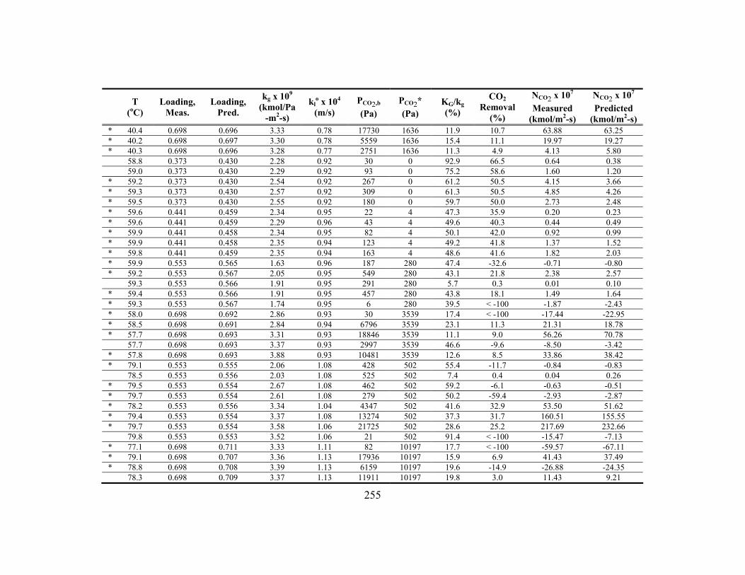
255
T (oC)
Loading, Meas.
Loading, Pred.
kg x 109 (kmol/Pa
-m2-s)
klo x 104 (m/s)
PCO2,b (Pa)
PCO2* (Pa)
KG/kg (%)
CO2 Removal
(%)
NCO2 x 107 Measured
(kmol/m2-s)
NCO2 x 107 Predicted
(kmol/m2-s) * 40.4 0.698 0.696 3.33 0.78 17730 1636 11.9 10.7 63.88 63.25 * 40.2 0.698 0.697 3.30 0.78 5559 1636 15.4 11.1 19.97 19.27 * 40.3 0.698 0.696 3.28 0.77 2751 1636 11.3 4.9 4.13 5.80 58.8 0.373 0.430 2.28 0.92 30 0 92.9 66.5 0.64 0.38 59.0 0.373 0.430 2.29 0.92 93 0 75.2 58.6 1.60 1.20 * 59.2 0.373 0.430 2.54 0.92 267 0 61.2 50.5 4.15 3.66 * 59.3 0.373 0.430 2.57 0.92 309 0 61.3 50.5 4.85 4.26 * 59.5 0.373 0.430 2.55 0.92 180 0 59.7 50.0 2.73 2.48 * 59.6 0.441 0.459 2.34 0.95 22 4 47.3 35.9 0.20 0.23 * 59.6 0.441 0.459 2.29 0.96 43 4 49.6 40.3 0.44 0.49 * 59.9 0.441 0.458 2.34 0.95 82 4 50.1 42.0 0.92 0.99 * 59.9 0.441 0.458 2.35 0.94 123 4 49.2 41.8 1.37 1.52 * 59.8 0.441 0.459 2.35 0.94 163 4 48.6 41.6 1.82 2.03 * 59.9 0.553 0.565 1.63 0.96 187 280 47.4 -32.6 -0.71 -0.80 * 59.2 0.553 0.567 2.05 0.95 549 280 43.1 21.8 2.38 2.57 59.3 0.553 0.566 1.91 0.95 291 280 5.7 0.3 0.01 0.10 * 59.4 0.553 0.566 1.91 0.95 457 280 43.8 18.1 1.49 1.64 * 59.3 0.553 0.567 1.74 0.95 6 280 39.5 < -100 -1.87 -2.43 * 58.0 0.698 0.692 2.86 0.93 30 3539 17.4 < -100 -17.44 -22.95 * 58.5 0.698 0.691 2.84 0.94 6796 3539 23.1 11.3 21.31 18.78 * 57.7 0.698 0.693 3.31 0.93 18846 3539 11.1 9.0 56.26 70.78 57.7 0.698 0.693 3.37 0.93 2997 3539 46.6 -9.6 -8.50 -3.42 * 57.8 0.698 0.693 3.88 0.93 10481 3539 12.6 8.5 33.86 38.42 * 79.1 0.553 0.555 2.06 1.08 428 502 55.4 -11.7 -0.84 -0.83 78.5 0.553 0.556 2.03 1.08 525 502 7.4 0.4 0.04 0.26 * 79.5 0.553 0.554 2.67 1.08 462 502 59.2 -6.1 -0.63 -0.51 * 79.7 0.553 0.554 2.61 1.08 279 502 50.2 -59.4 -2.93 -2.87 * 78.2 0.553 0.556 3.34 1.04 4347 502 41.6 32.9 53.50 51.62 * 79.4 0.553 0.554 3.37 1.08 13274 502 37.3 31.7 160.51 155.55 * 79.7 0.553 0.554 3.58 1.06 21725 502 28.6 25.2 217.69 232.66 79.8 0.553 0.553 3.52 1.06 21 502 91.4 < -100 -15.47 -7.13 * 77.1 0.698 0.711 3.33 1.11 82 10197 17.7 < -100 -59.57 -67.11 * 79.1 0.698 0.707 3.36 1.13 17936 10197 15.9 6.9 41.43 37.49 * 78.8 0.698 0.708 3.39 1.13 6159 10197 19.6 -14.9 -26.88 -24.35 78.3 0.698 0.709 3.37 1.13 11911 10197 19.8 3.0 11.43 9.21
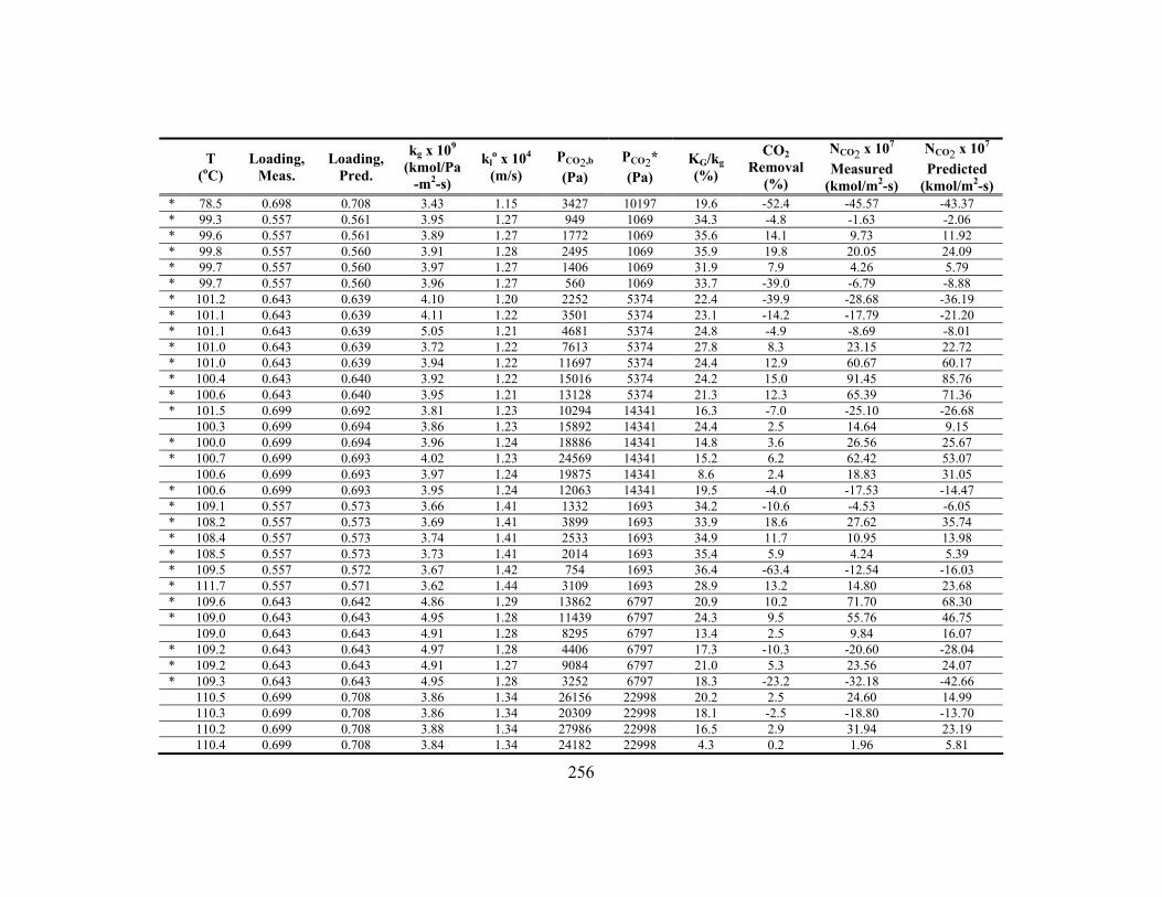
256
T (oC)
Loading, Meas.
Loading, Pred.
kg x 109 (kmol/Pa
-m2-s)
klo x 104 (m/s)
PCO2,b (Pa)
PCO2* (Pa)
KG/kg (%)
CO2 Removal
(%)
NCO2 x 107 Measured
(kmol/m2-s)
NCO2 x 107 Predicted
(kmol/m2-s) * 78.5 0.698 0.708 3.43 1.15 3427 10197 19.6 -52.4 -45.57 -43.37 * 99.3 0.557 0.561 3.95 1.27 949 1069 34.3 -4.8 -1.63 -2.06 * 99.6 0.557 0.561 3.89 1.27 1772 1069 35.6 14.1 9.73 11.92 * 99.8 0.557 0.560 3.91 1.28 2495 1069 35.9 19.8 20.05 24.09 * 99.7 0.557 0.560 3.97 1.27 1406 1069 31.9 7.9 4.26 5.79 * 99.7 0.557 0.560 3.96 1.27 560 1069 33.7 -39.0 -6.79 -8.88 * 101.2 0.643 0.639 4.10 1.20 2252 5374 22.4 -39.9 -28.68 -36.19 * 101.1 0.643 0.639 4.11 1.22 3501 5374 23.1 -14.2 -17.79 -21.20 * 101.1 0.643 0.639 5.05 1.21 4681 5374 24.8 -4.9 -8.69 -8.01 * 101.0 0.643 0.639 3.72 1.22 7613 5374 27.8 8.3 23.15 22.72 * 101.0 0.643 0.639 3.94 1.22 11697 5374 24.4 12.9 60.67 60.17 * 100.4 0.643 0.640 3.92 1.22 15016 5374 24.2 15.0 91.45 85.76 * 100.6 0.643 0.640 3.95 1.21 13128 5374 21.3 12.3 65.39 71.36 * 101.5 0.699 0.692 3.81 1.23 10294 14341 16.3 -7.0 -25.10 -26.68 100.3 0.699 0.694 3.86 1.23 15892 14341 24.4 2.5 14.64 9.15 * 100.0 0.699 0.694 3.96 1.24 18886 14341 14.8 3.6 26.56 25.67 * 100.7 0.699 0.693 4.02 1.23 24569 14341 15.2 6.2 62.42 53.07 100.6 0.699 0.693 3.97 1.24 19875 14341 8.6 2.4 18.83 31.05 * 100.6 0.699 0.693 3.95 1.24 12063 14341 19.5 -4.0 -17.53 -14.47 * 109.1 0.557 0.573 3.66 1.41 1332 1693 34.2 -10.6 -4.53 -6.05 * 108.2 0.557 0.573 3.69 1.41 3899 1693 33.9 18.6 27.62 35.74 * 108.4 0.557 0.573 3.74 1.41 2533 1693 34.9 11.7 10.95 13.98 * 108.5 0.557 0.573 3.73 1.41 2014 1693 35.4 5.9 4.24 5.39 * 109.5 0.557 0.572 3.67 1.42 754 1693 36.4 -63.4 -12.54 -16.03 * 111.7 0.557 0.571 3.62 1.44 3109 1693 28.9 13.2 14.80 23.68 * 109.6 0.643 0.642 4.86 1.29 13862 6797 20.9 10.2 71.70 68.30 * 109.0 0.643 0.643 4.95 1.28 11439 6797 24.3 9.5 55.76 46.75 109.0 0.643 0.643 4.91 1.28 8295 6797 13.4 2.5 9.84 16.07 * 109.2 0.643 0.643 4.97 1.28 4406 6797 17.3 -10.3 -20.60 -28.04 * 109.2 0.643 0.643 4.91 1.27 9084 6797 21.0 5.3 23.56 24.07 * 109.3 0.643 0.643 4.95 1.28 3252 6797 18.3 -23.2 -32.18 -42.66 110.5 0.699 0.708 3.86 1.34 26156 22998 20.2 2.5 24.60 14.99 110.3 0.699 0.708 3.86 1.34 20309 22998 18.1 -2.5 -18.80 -13.70 110.2 0.699 0.708 3.88 1.34 27986 22998 16.5 2.9 31.94 23.19 110.4 0.699 0.708 3.84 1.34 24182 22998 4.3 0.2 1.96 5.81

257
T (oC)
Loading, Meas.
Loading, Pred.
kg x 109 (kmol/Pa
-m2-s)
klo x 104 (m/s)
PCO2,b (Pa)
PCO2* (Pa)
KG/kg (%)
CO2 Removal
(%)
NCO2 x 107 Measured
(kmol/m2-s)
NCO2 x 107 Predicted
(kmol/m2-s) * 110.2 0.699 0.709 3.84 1.33 18545 22998 14.9 -3.8 -25.54 -23.34 * 110.4 0.699 0.708 3.86 1.34 14760 22998 10.9 -6.7 -34.80 -45.81 3.6 m K+/1.8 m PZ * 41.3 0.610 0.563 3.33 0.66 4401 157 32.3 28.7 45.64 49.08 * 41.7 0.610 0.561 3.34 0.66 13843 157 27.1 24.7 124.10 141.77 * 41.2 0.610 0.563 3.30 0.67 3 157 32.6 < -100 -1.65 -1.87 * 41.5 0.610 0.562 3.31 0.67 9196 157 28.8 26.2 86.18 98.76 * 41.5 0.610 0.562 3.35 0.67 6738 157 29.7 26.9 65.56 74.43 * 60.3 0.610 0.610 3.09 0.81 9499 1544 42.5 31.8 104.36 81.95 * 61.7 0.610 0.605 3.07 0.82 4933 1544 36.4 23.8 37.81 38.08 * 61.6 0.610 0.605 3.04 0.82 27 1544 36.3 < -100 -16.74 -18.07 * 63.0 0.610 0.600 3.30 0.84 13565 1544 37.9 30.0 150.20 126.57 * 59.1 0.735 0.727 3.03 0.77 94 12829 16.1 < -100 -62.16 -66.90 * 59.4 0.735 0.726 3.03 0.77 25739 12829 14.5 7.2 56.68 43.10 59.1 0.735 0.727 2.95 0.76 12034 12829 -24.1 1.7 5.66 -3.24 * 58.8 0.735 0.728 2.94 0.76 19702 12829 12.8 4.6 25.91 24.62 * 59.2 0.735 0.727 2.96 0.76 29217 12829 14.3 7.9 69.48 51.39 * 59.1 0.761 0.787 3.15 0.77 20819 36714 7.6 -6.3 -38.17 -31.95 59.3 0.761 0.786 3.14 0.76 34830 36714 5.3 -0.3 -3.11 -3.10 59.4 0.761 0.785 3.11 0.77 46321 36714 2.1 0.4 6.32 14.38 58.9 0.761 0.788 3.00 0.76 53645 36714 4.6 1.4 23.20 23.14 59.2 0.761 0.786 2.84 0.76 60056 36714 8.2 3.0 54.30 30.24 * 78.9 0.610 0.623 3.25 1.00 14758 5590 31.7 18.8 94.65 83.40 79.1 0.610 0.622 3.25 1.00 5382 5590 51.2 -2.2 -3.46 -2.11 * 79.0 0.610 0.622 3.22 1.00 10218 5590 28.9 13.1 43.18 44.97 * 79.6 0.610 0.621 3.17 1.00 76 5590 29.9 < -100 -52.27 -62.23 * 79.4 0.610 0.621 3.27 1.00 7744 5590 30.7 8.8 21.61 21.91 3.6 m K+/3.6 m PZ * 40.1 0.560 0.579 2.78 0.58 2247 371 52.5 38.6 27.35 20.51 * 40.1 0.560 0.579 2.77 0.58 1005 371 38.7 23.9 6.80 7.02 * 40.5 0.560 0.575 2.74 0.59 4967 371 47.9 38.7 60.45 49.26 * 40.9 0.560 0.571 2.77 0.59 16183 371 38.2 33.1 167.54 153.76 * 41.1 0.560 0.570 2.74 0.59 10636 371 41.4 35.3 116.36 105.86 * 42.0 0.684 0.681 2.55 0.60 8814 1711 34.7 26.3 63.00 47.05 * 41.0 0.684 0.687 2.56 0.59 2636 1711 41.9 15.0 9.93 6.46

258
T (oC)
Loading, Meas.
Loading, Pred.
kg x 109 (kmol/Pa
-m2-s)
klo x 104 (m/s)
PCO2,b (Pa)
PCO2* (Pa)
KG/kg (%)
CO2 Removal
(%)
NCO2 x 107 Measured
(kmol/m2-s)
NCO2 x 107 Predicted
(kmol/m2-s) * 41.2 0.684 0.686 2.60 0.60 1146 1711 43.5 -27.4 -6.38 -4.08 * 40.3 0.684 0.690 2.95 0.58 19567 1711 19.7 17.2 103.62 96.90 * 40.8 0.684 0.688 2.97 0.59 13620 1711 22.5 19.0 79.55 72.21 58.4 0.500 0.421 2.17 0.72 216 201 35.3 2.8 0.11 0.20 * 58.0 0.500 0.422 2.16 0.72 237 201 68.5 11.5 0.53 0.48 * 58.2 0.500 0.421 2.10 0.72 146 201 60.4 -30.7 -0.70 -0.72 * 59.4 0.500 0.418 2.18 0.73 371 201 60.1 27.4 2.23 2.29 * 59.0 0.500 0.419 2.17 0.73 460 201 60.7 32.6 3.42 3.46 * 59.2 0.500 0.418 2.16 0.72 420 201 59.3 30.1 2.80 2.93 * 60.8 0.560 0.506 2.70 0.75 5084 1209 57.8 38.7 60.45 51.65 * 60.5 0.560 0.508 2.72 0.75 1444 1209 59.3 10.3 3.79 3.23 * 61.0 0.560 0.505 2.64 0.75 2542 1209 58.5 29.1 20.58 17.92 * 60.6 0.560 0.507 2.69 0.75 10696 1209 48.4 37.5 123.46 120.87 * 60.2 0.560 0.510 2.67 0.75 16249 1209 47.5 37.8 191.02 182.37 * 60.4 0.560 0.509 2.70 0.75 13336 1209 48.3 38.0 158.34 151.39 59.2 0.652 0.674 2.86 0.74 5979 6869 22.8 -3.8 -5.81 -6.72 59.6 0.652 0.672 2.88 0.74 8872 6869 20.7 5.0 11.97 14.85 59.6 0.652 0.672 2.88 0.74 7411 6869 25.7 2.0 4.03 4.14 * 60.4 0.652 0.667 2.96 0.75 14372 6869 20.1 10.7 44.72 53.28 * 60.5 0.652 0.666 2.96 0.74 20047 6869 20.7 13.4 80.66 86.82 * 60.8 0.652 0.665 2.94 0.74 17416 6869 18.5 11.2 57.27 72.42 77.7 0.554 0.545 2.64 0.88 6676 7323 27.7 -3.0 -4.73 -6.85 * 78.0 0.554 0.543 2.63 0.89 3615 7323 30.7 -42.1 -29.92 -40.88 * 79.5 0.554 0.534 2.64 0.89 12730 7323 30.2 13.0 43.06 54.94 * 79.1 0.554 0.536 2.63 0.89 18628 7323 34.1 19.9 101.38 108.42 * 78.9 0.554 0.538 2.83 0.88 15024 7323 23.6 12.3 51.55 77.88 * 79.1 0.684 0.679 2.92 0.86 10461 34574 11.9 -34.7 -84.23 -123.45 * 79.1 0.684 0.679 2.88 0.85 19868 34574 13.0 -10.7 -55.14 -66.87 79.2 0.684 0.678 3.66 0.87 29142 34574 18.6 -4.7 -37.03 -23.41 79.7 0.684 0.675 2.95 0.87 37965 34574 17.8 1.6 17.77 13.37 * 79.7 0.684 0.675 2.88 0.87 50856 34574 13.8 4.3 64.68 57.12 4.8 m K+/0.6 m PZ * 41.1 0.717 0.716 3.33 0.69 4946 2453 15.6 8.1 12.93 10.15 * 41.0 0.717 0.716 3.31 0.68 10222 2453 11.1 8.6 28.69 28.12 39.9 0.717 0.720 3.41 0.69 2845 2453 15.2 2.2 2.03 1.63
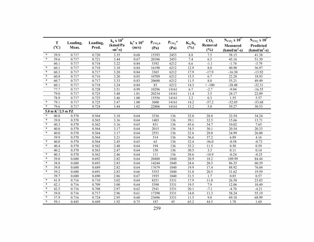
259
T (oC)
Loading, Meas.
Loading, Pred.
kg x 109 (kmol/Pa
-m2-s)
klo x 104 (m/s)
PCO2,b (Pa)
PCO2* (Pa)
KG/kg (%)
CO2 Removal
(%)
NCO2 x 107 Measured
(kmol/m2-s)
NCO2 x 107 Predicted
(kmol/m2-s) * 39.9 0.717 0.720 3.35 0.68 15393 2453 8.8 7.5 38.15 41.38 * 39.6 0.717 0.721 3.44 0.67 20106 2453 7.4 6.5 45.16 51.30 60.1 0.717 0.718 3.22 0.84 5392 6212 6.6 -1.1 -1.74 -3.79 * 60.1 0.717 0.718 3.18 0.84 16190 6212 12.9 8.0 40.90 36.97 * 60.3 0.717 0.717 3.20 0.84 3365 6212 17.9 -17.9 -16.30 -13.92 * 60.8 0.717 0.716 3.20 0.85 10709 6212 15.5 6.7 22.28 18.93 * 60.7 0.717 0.717 3.33 0.83 20680 6212 11.5 8.0 55.21 49.49 * 60.1 0.717 0.718 3.24 0.84 83 6212 14.3 < -100 -28.48 -32.31 77.7 0.717 0.728 3.51 0.99 10296 14161 6.7 -2.7 -9.04 -16.55 79.0 0.717 0.725 3.48 1.01 20234 14161 11.4 3.5 24.17 22.09 78.9 0.717 0.725 3.46 1.00 15556 14161 3.2 0.3 1.55 5.57 * 79.1 0.717 0.725 3.47 1.00 3600 14161 14.2 -57.2 -52.05 -53.68 * 79.6 0.717 0.724 3.44 1.02 22806 14161 13.2 5.0 39.27 30.53 5.0 m K+/2.5 m PZ * 40.0 0.570 0.564 3.18 0.64 3336 136 32.0 28.8 32.54 34.24 * 39.8 0.570 0.565 3.16 0.64 1403 136 39.1 32.5 15.66 13.71 * 40.3 0.570 0.562 3.16 0.65 831 136 45.6 34.7 10.02 7.65 * 40.0 0.570 0.564 3.17 0.64 2015 136 34.5 30.1 20.54 20.33 * 40.0 0.570 0.564 3.17 0.64 2551 136 32.6 29.0 24.99 26.00 39.9 0.570 0.564 3.21 0.64 514 136 56.6 37.2 6.89 4.16 * 40.0 0.570 0.564 2.45 0.65 63 136 32.4 -56.0 -0.58 -0.73 * 40.4 0.570 0.562 2.48 0.64 194 136 35.2 11.5 0.50 0.59 40.2 0.570 0.563 2.47 0.64 150 136 30.5 3.3 0.11 0.14 * 40.3 0.570 0.562 2.46 0.64 111 136 38.6 -10.9 -0.24 -0.25 * 39.0 0.680 0.692 2.82 0.64 20488 1840 20.9 18.2 109.99 84.44 * 38.8 0.680 0.693 2.83 0.64 14244 1840 24.6 20.5 86.35 60.39 * 39.8 0.680 0.689 2.82 0.64 17679 1840 19.9 17.4 88.92 76.04 * 39.2 0.680 0.691 2.83 0.66 5353 1840 31.8 20.5 31.62 19.59 39.7 0.680 0.690 2.86 0.67 1935 1840 31.5 1.7 0.85 0.57 * 41.9 0.716 0.710 3.02 0.64 8251 3331 17.9 11.0 26.58 23.83 * 42.1 0.716 0.709 3.00 0.64 5398 3331 19.5 7.9 12.06 10.49 * 42.5 0.716 0.708 2.97 0.62 2541 3331 20.1 -7.1 -4.70 -4.21 * 39.8 0.716 0.717 2.96 0.61 17398 3331 14.0 11.3 58.24 55.19 * 37.9 0.716 0.724 2.95 0.60 23696 3331 11.5 9.8 69.10 68.99 * 59.1 0.445 0.449 1.92 0.75 187 45 65.2 44.5 1.78 1.69

260
T (oC)
Loading, Meas.
Loading, Pred.
kg x 109 (kmol/Pa
-m2-s)
klo x 104 (m/s)
PCO2,b (Pa)
PCO2* (Pa)
KG/kg (%)
CO2 Removal
(%)
NCO2 x 107 Measured
(kmol/m2-s)
NCO2 x 107 Predicted
(kmol/m2-s) * 60.2 0.445 0.446 1.88 0.76 114 45 61.9 36.2 0.81 0.82 * 60.4 0.445 0.446 1.92 0.74 138 45 63.9 40.4 1.14 1.12 60.8 0.445 0.445 1.91 0.74 44 45 40.0 -1.5 -0.01 -0.01 * 60.5 0.445 0.445 1.89 0.75 27 45 50.0 -52.4 -0.17 -0.21 * 61.5 0.445 0.443 1.89 0.75 22 45 71.6 -134.8 -0.31 -0.28 * 59.6 0.472 0.454 2.96 0.81 3675 56 61.5 49.0 65.89 54.21 * 59.5 0.472 0.454 2.95 0.81 1850 56 63.0 49.5 33.33 27.00 * 59.6 0.472 0.454 2.98 0.81 6455 56 58.5 47.2 111.43 95.04 * 59.9 0.472 0.454 2.99 0.81 8292 56 57.3 46.4 141.29 121.93 * 60.6 0.472 0.452 2.97 0.82 4314 56 60.6 48.5 76.68 64.36 * 60.5 0.472 0.452 2.96 0.81 2438 56 62.5 49.4 44.02 36.18 * 61.9 0.595 0.606 2.63 0.81 7699 1642 46.2 33.0 73.55 60.61 * 60.3 0.595 0.611 3.02 0.80 4349 1642 42.0 25.1 34.32 28.42 * 60.3 0.595 0.611 3.02 0.80 10878 1642 37.3 29.2 104.06 90.78 * 60.3 0.595 0.611 3.01 0.81 2579 1642 35.9 13.5 10.12 10.02 * 60.4 0.595 0.611 3.03 0.80 13045 1642 35.9 28.8 124.02 109.93 * 60.1 0.595 0.612 3.05 0.80 7683 1642 38.7 28.4 71.29 61.25 * 59.3 0.602 0.619 3.04 0.78 1452 1778 24.4 -6.3 -2.42 -3.38 * 60.4 0.602 0.615 3.01 0.78 4343 1778 32.4 19.1 25.04 26.37 * 59.3 0.602 0.619 3.03 0.77 914 1778 34.9 -44.4 -9.12 -9.00 * 59.6 0.602 0.618 3.02 0.78 6620 1778 32.6 23.1 47.70 47.83 * 59.9 0.602 0.617 3.05 0.77 10681 1778 31.3 24.7 84.99 84.82 * 60.8 0.602 0.614 3.04 0.78 8456 1778 29.3 22.3 59.48 66.45 * 59.5 0.652 0.660 2.95 0.79 16845 4081 24.6 18.1 92.50 86.37 * 59.8 0.652 0.659 3.03 0.79 21243 4081 30.8 23.1 160.11 111.49 * 60.4 0.652 0.657 2.98 0.77 26130 4081 25.1 20.0 165.11 135.31 * 59.5 0.652 0.660 2.96 0.80 2866 4081 29.8 -15.1 -10.71 -9.86 * 59.1 0.652 0.662 2.97 0.79 5562 4081 32.2 9.0 14.19 11.46 * 59.8 0.652 0.659 2.98 0.79 13720 4081 28.4 19.3 81.46 68.41 59.4 0.703 0.701 3.14 0.74 11394 9467 7.0 1.3 4.25 9.84 59.3 0.703 0.701 3.17 0.73 8381 9467 7.5 -1.1 -2.57 -5.79 59.3 0.703 0.701 3.10 0.75 14135 9467 10.8 3.7 15.66 22.85 * 59.0 0.703 0.702 2.83 0.76 21772 9467 14.2 8.2 49.52 53.69 * 59.2 0.703 0.702 3.11 0.76 25674 9467 12.1 7.6 60.98 68.33 * 58.9 0.703 0.702 3.12 0.77 27982 9467 11.3 7.4 65.00 75.85
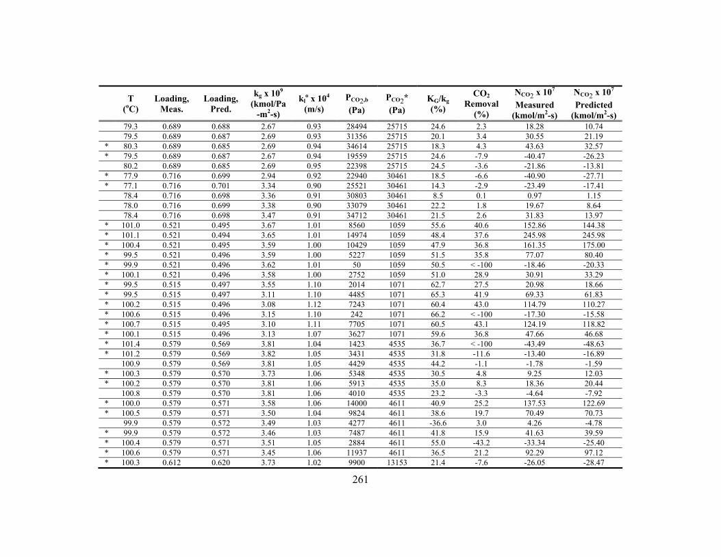
261
T (oC)
Loading, Meas.
Loading, Pred.
kg x 109 (kmol/Pa
-m2-s)
klo x 104 (m/s)
PCO2,b (Pa)
PCO2* (Pa)
KG/kg (%)
CO2 Removal
(%)
NCO2 x 107 Measured
(kmol/m2-s)
NCO2 x 107 Predicted
(kmol/m2-s) 79.3 0.689 0.688 2.67 0.93 28494 25715 24.6 2.3 18.28 10.74 79.5 0.689 0.687 2.69 0.93 31356 25715 20.1 3.4 30.55 21.19 * 80.3 0.689 0.685 2.69 0.94 34614 25715 18.3 4.3 43.63 32.57 * 79.5 0.689 0.687 2.67 0.94 19559 25715 24.6 -7.9 -40.47 -26.23 80.2 0.689 0.685 2.69 0.95 22398 25715 24.5 -3.6 -21.86 -13.81 * 77.9 0.716 0.699 2.94 0.92 22940 30461 18.5 -6.6 -40.90 -27.71 * 77.1 0.716 0.701 3.34 0.90 25521 30461 14.3 -2.9 -23.49 -17.41 78.4 0.716 0.698 3.36 0.91 30803 30461 8.5 0.1 0.97 1.15 78.0 0.716 0.699 3.38 0.90 33079 30461 22.2 1.8 19.67 8.64 78.4 0.716 0.698 3.47 0.91 34712 30461 21.5 2.6 31.83 13.97 * 101.0 0.521 0.495 3.67 1.01 8560 1059 55.6 40.6 152.86 144.38 * 101.1 0.521 0.494 3.65 1.01 14974 1059 48.4 37.6 245.98 245.98 * 100.4 0.521 0.495 3.59 1.00 10429 1059 47.9 36.8 161.35 175.00 * 99.5 0.521 0.496 3.59 1.00 5227 1059 51.5 35.8 77.07 80.40 * 99.9 0.521 0.496 3.62 1.01 50 1059 50.5 < -100 -18.46 -20.33 * 100.1 0.521 0.496 3.58 1.00 2752 1059 51.0 28.9 30.91 33.29 * 99.5 0.515 0.497 3.55 1.10 2014 1071 62.7 27.5 20.98 18.66 * 99.5 0.515 0.497 3.11 1.10 4485 1071 65.3 41.9 69.33 61.83 * 100.2 0.515 0.496 3.08 1.12 7243 1071 60.4 43.0 114.79 110.27 * 100.6 0.515 0.496 3.15 1.10 242 1071 66.2 < -100 -17.30 -15.58 * 100.7 0.515 0.495 3.10 1.11 7705 1071 60.5 43.1 124.19 118.82 * 100.1 0.515 0.496 3.13 1.07 3627 1071 59.6 36.8 47.66 46.68 * 101.4 0.579 0.569 3.81 1.04 1423 4535 36.7 < -100 -43.49 -48.63 * 101.2 0.579 0.569 3.82 1.05 3431 4535 31.8 -11.6 -13.40 -16.89 100.9 0.579 0.569 3.81 1.05 4429 4535 44.2 -1.1 -1.78 -1.59 * 100.3 0.579 0.570 3.73 1.06 5348 4535 30.5 4.8 9.25 12.03 * 100.2 0.579 0.570 3.81 1.06 5913 4535 35.0 8.3 18.36 20.44 100.8 0.579 0.570 3.81 1.06 4010 4535 23.2 -3.3 -4.64 -7.92 * 100.0 0.579 0.571 3.58 1.06 14000 4611 40.9 25.2 137.53 122.69 * 100.5 0.579 0.571 3.50 1.04 9824 4611 38.6 19.7 70.49 70.73 99.9 0.579 0.572 3.49 1.03 4277 4611 -36.6 3.0 4.26 -4.78 * 99.9 0.579 0.572 3.46 1.03 7487 4611 41.8 15.9 41.63 39.59 * 100.4 0.579 0.571 3.51 1.05 2884 4611 55.0 -43.2 -33.34 -25.40 * 100.6 0.579 0.571 3.45 1.06 11937 4611 36.5 21.2 92.29 97.12 * 100.3 0.612 0.620 3.73 1.02 9900 13153 21.4 -7.6 -26.05 -28.47
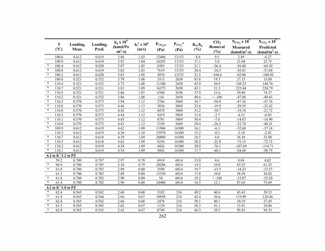
262
T (oC)
Loading, Meas.
Loading, Pred.
kg x 109 (kmol/Pa
-m2-s)
klo x 104 (m/s)
PCO2,b (Pa)
PCO2* (Pa)
KG/kg (%)
CO2 Removal
(%)
NCO2 x 107 Measured
(kmol/m2-s)
NCO2 x 107 Predicted
(kmol/m2-s) 100.6 0.612 0.619 3.86 1.03 12406 13153 -8.6 0.5 2.49 -6.27 100.9 0.612 0.619 3.92 1.04 16285 13153 17.1 3.0 21.04 25.73 * 100.4 0.612 0.620 3.87 1.02 6305 13153 21.1 -26.4 -56.04 -64.30 * 100.8 0.612 0.619 3.82 1.03 7619 13153 20.4 -16.3 -43.01 -51.04 * 100.2 0.612 0.620 3.83 1.05 3076 13153 21.5 -104.6 -82.88 -100.50 109.8 0.521 0.532 3.78 1.08 3515 2658 83.8 19.7 27.15 15.88 * 110.4 0.521 0.532 3.73 1.08 11380 2658 45.9 30.9 149.25 148.76 * 110.7 0.521 0.531 3.81 1.09 16375 2658 43.1 31.3 225.44 224.79 * 110.5 0.521 0.531 3.86 1.07 6760 2658 37.9 21.6 59.89 74.37 * 110.2 0.521 0.532 3.86 1.08 110 2658 48.6 < -100 -47.86 -49.43 * 110.5 0.570 0.573 3.94 1.12 2766 5869 38.7 -58.8 -47.36 -47.76 * 110.8 0.570 0.573 4.46 1.13 3836 5869 32.6 -19.9 -29.55 -32.42 * 110.0 0.570 0.573 4.42 1.12 4478 5869 31.2 -10.7 -19.18 -21.72 110.2 0.570 0.573 4.44 1.12 5419 5869 31.0 -2.7 -6.21 -6.85 * 110.1 0.570 0.573 4.43 1.12 4781 5869 30.4 -7.6 -14.67 -16.90 * 110.0 0.570 0.573 4.41 1.12 3338 5869 29.4 -26.5 -32.74 -40.21 * 109.9 0.612 0.619 4.62 1.09 11906 16300 16.1 -6.3 -32.60 -37.14 110.2 0.612 0.619 4.36 1.10 15970 16300 15.2 -0.3 -2.18 -2.42 * 110.7 0.612 0.618 4.39 1.09 20809 16300 18.5 4.0 36.58 32.88 * 110.5 0.612 0.618 4.62 1.09 8256 16300 20.2 -22.8 -75.15 -72.75 * 110.2 0.612 0.619 4.54 1.09 4426 16300 20.0 -76.1 -107.69 -114.71 * 110.1 0.612 0.619 4.54 1.09 5802 16300 17.7 -40.1 -84.60 -98.79 6.2 m K+/1.2 m PZ 59.2 0.700 0.707 2.97 0.78 6918 6014 33.0 4.6 8.84 4.62 * 60.4 0.700 0.705 3.10 0.79 20286 6014 14.3 10.0 63.25 61.25 * 61.0 0.700 0.703 2.98 0.80 3590 6014 19.7 -15.5 -14.23 -13.57 61.3 0.700 0.703 2.88 0.80 13520 6014 17.8 10.0 38.58 36.02 * 61.0 0.700 0.703 2.90 0.80 54 6014 19.2 < -100 -33.07 -35.20 * 61.4 0.700 0.702 2.90 0.80 24400 6014 16.5 12.1 87.65 75.69 6.2 m K+/1.8 m PZ * 62.4 0.565 0.542 2.68 0.68 5182 216 49.2 40.8 65.43 59.33 * 61.8 0.565 0.544 2.66 0.67 10858 216 42.4 36.6 119.99 120.46 * 62.4 0.565 0.542 2.66 0.68 2478 216 50.1 40.1 30.19 27.45 * 61.5 0.565 0.545 2.62 0.67 1129 216 58.3 41.1 13.91 10.96 * 62.0 0.565 0.543 2.42 0.67 8749 216 46.3 39.5 95.83 94.53
263
Appendix D: Tabulated Model Predictions
D.1. PCO2* and Speciation Predictions
This section presents ENRTL model predictions of bulk solution equilibrium as
determined from 1H NMR and PCO2* experiments outlined in Chapter 5. The data
represent model results given the nominal solution conditions listed in the captions.
The equilibrium partial pressure is reported in Pa and the liquid concentrations are
given in mol/kg-H2O (m). Loading is given in mol CO2/(mol K+ + mol PZ).
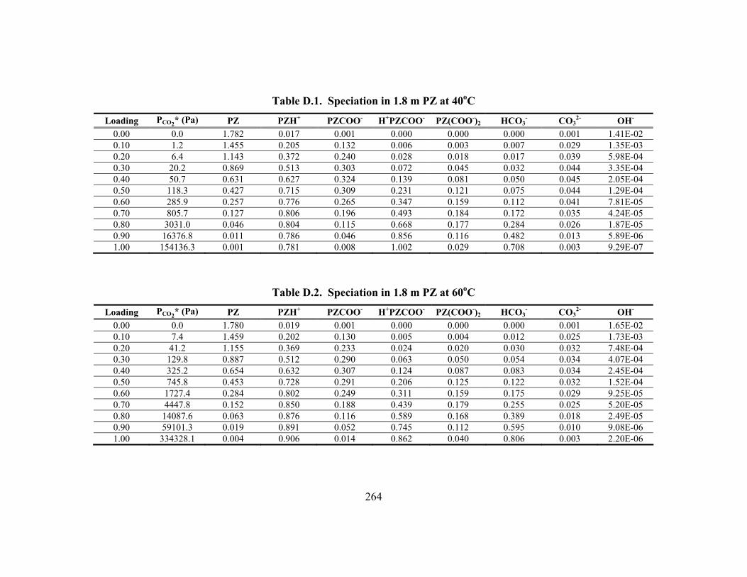
264
Table D.1. Speciation in 1.8 m PZ at 40oC
Loading PCO2* (Pa) PZ PZH+ PZCOO- H+PZCOO- PZ(COO-)2 HCO3- CO3
2- OH-
0.00 0.0 1.782 0.017 0.001 0.000 0.000 0.000 0.001 1.41E-02 0.10 1.2 1.455 0.205 0.132 0.006 0.003 0.007 0.029 1.35E-03 0.20 6.4 1.143 0.372 0.240 0.028 0.018 0.017 0.039 5.98E-04 0.30 20.2 0.869 0.513 0.303 0.072 0.045 0.032 0.044 3.35E-04 0.40 50.7 0.631 0.627 0.324 0.139 0.081 0.050 0.045 2.05E-04 0.50 118.3 0.427 0.715 0.309 0.231 0.121 0.075 0.044 1.29E-04 0.60 285.9 0.257 0.776 0.265 0.347 0.159 0.112 0.041 7.81E-05 0.70 805.7 0.127 0.806 0.196 0.493 0.184 0.172 0.035 4.24E-05 0.80 3031.0 0.046 0.804 0.115 0.668 0.177 0.284 0.026 1.87E-05 0.90 16376.8 0.011 0.786 0.046 0.856 0.116 0.482 0.013 5.89E-06 1.00 154136.3 0.001 0.781 0.008 1.002 0.029 0.708 0.003 9.29E-07
Table D.2. Speciation in 1.8 m PZ at 60oC
Loading PCO2* (Pa) PZ PZH+ PZCOO- H+PZCOO- PZ(COO-)2 HCO3- CO3
2- OH-
0.00 0.0 1.780 0.019 0.001 0.000 0.000 0.000 0.001 1.65E-02 0.10 7.4 1.459 0.202 0.130 0.005 0.004 0.012 0.025 1.73E-03 0.20 41.2 1.155 0.369 0.233 0.024 0.020 0.030 0.032 7.48E-04 0.30 129.8 0.887 0.512 0.290 0.063 0.050 0.054 0.034 4.07E-04 0.40 325.2 0.654 0.632 0.307 0.124 0.087 0.083 0.034 2.45E-04 0.50 745.8 0.453 0.728 0.291 0.206 0.125 0.122 0.032 1.52E-04 0.60 1727.4 0.284 0.802 0.249 0.311 0.159 0.175 0.029 9.25E-05 0.70 4447.8 0.152 0.850 0.188 0.439 0.179 0.255 0.025 5.20E-05 0.80 14087.6 0.063 0.876 0.116 0.589 0.168 0.389 0.018 2.49E-05 0.90 59101.3 0.019 0.891 0.052 0.745 0.112 0.595 0.010 9.08E-06 1.00 334328.1 0.004 0.906 0.014 0.862 0.040 0.806 0.003 2.20E-06
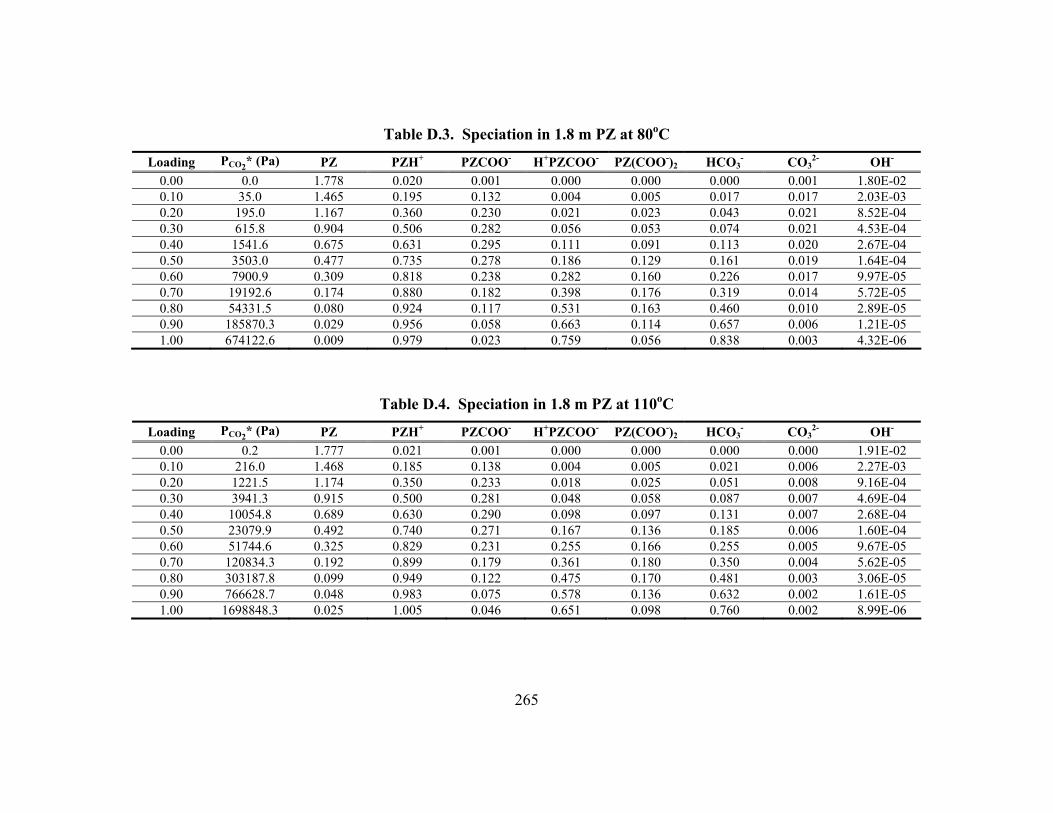
265
Table D.3. Speciation in 1.8 m PZ at 80oC
Loading PCO2* (Pa) PZ PZH+ PZCOO- H+PZCOO- PZ(COO-)2 HCO3- CO3
2- OH-
0.00 0.0 1.778 0.020 0.001 0.000 0.000 0.000 0.001 1.80E-02 0.10 35.0 1.465 0.195 0.132 0.004 0.005 0.017 0.017 2.03E-03 0.20 195.0 1.167 0.360 0.230 0.021 0.023 0.043 0.021 8.52E-04 0.30 615.8 0.904 0.506 0.282 0.056 0.053 0.074 0.021 4.53E-04 0.40 1541.6 0.675 0.631 0.295 0.111 0.091 0.113 0.020 2.67E-04 0.50 3503.0 0.477 0.735 0.278 0.186 0.129 0.161 0.019 1.64E-04 0.60 7900.9 0.309 0.818 0.238 0.282 0.160 0.226 0.017 9.97E-05 0.70 19192.6 0.174 0.880 0.182 0.398 0.176 0.319 0.014 5.72E-05 0.80 54331.5 0.080 0.924 0.117 0.531 0.163 0.460 0.010 2.89E-05 0.90 185870.3 0.029 0.956 0.058 0.663 0.114 0.657 0.006 1.21E-05 1.00 674122.6 0.009 0.979 0.023 0.759 0.056 0.838 0.003 4.32E-06
Table D.4. Speciation in 1.8 m PZ at 110oC
Loading PCO2* (Pa) PZ PZH+ PZCOO- H+PZCOO- PZ(COO-)2 HCO3- CO3
2- OH-
0.00 0.2 1.777 0.021 0.001 0.000 0.000 0.000 0.000 1.91E-02 0.10 216.0 1.468 0.185 0.138 0.004 0.005 0.021 0.006 2.27E-03 0.20 1221.5 1.174 0.350 0.233 0.018 0.025 0.051 0.008 9.16E-04 0.30 3941.3 0.915 0.500 0.281 0.048 0.058 0.087 0.007 4.69E-04 0.40 10054.8 0.689 0.630 0.290 0.098 0.097 0.131 0.007 2.68E-04 0.50 23079.9 0.492 0.740 0.271 0.167 0.136 0.185 0.006 1.60E-04 0.60 51744.6 0.325 0.829 0.231 0.255 0.166 0.255 0.005 9.67E-05 0.70 120834.3 0.192 0.899 0.179 0.361 0.180 0.350 0.004 5.62E-05 0.80 303187.8 0.099 0.949 0.122 0.475 0.170 0.481 0.003 3.06E-05 0.90 766628.7 0.048 0.983 0.075 0.578 0.136 0.632 0.002 1.61E-05 1.00 1698848.3 0.025 1.005 0.046 0.651 0.098 0.760 0.002 8.99E-06
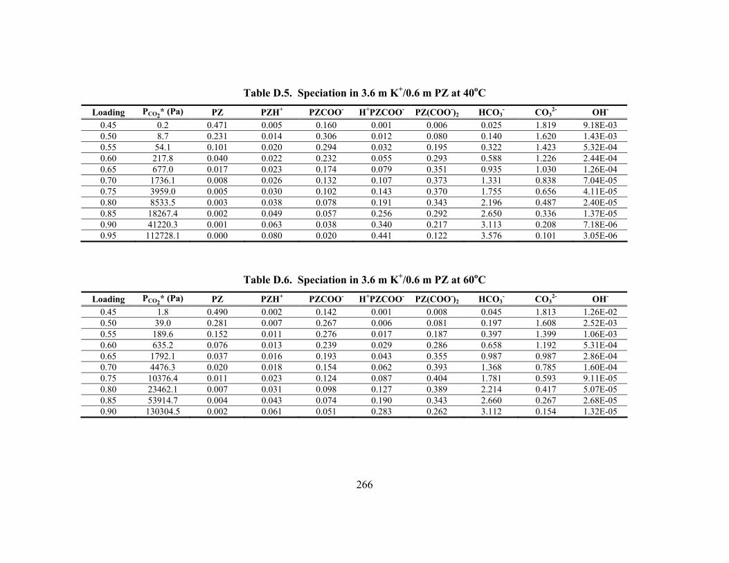
266
Table D.5. Speciation in 3.6 m K+/0.6 m PZ at 40oC
Loading PCO2* (Pa) PZ PZH+ PZCOO- H+PZCOO- PZ(COO-)2 HCO3- CO3
2- OH-
0.45 0.2 0.471 0.005 0.160 0.001 0.006 0.025 1.819 9.18E-03 0.50 8.7 0.231 0.014 0.306 0.012 0.080 0.140 1.620 1.43E-03 0.55 54.1 0.101 0.020 0.294 0.032 0.195 0.322 1.423 5.32E-04 0.60 217.8 0.040 0.022 0.232 0.055 0.293 0.588 1.226 2.44E-04 0.65 677.0 0.017 0.023 0.174 0.079 0.351 0.935 1.030 1.26E-04 0.70 1736.1 0.008 0.026 0.132 0.107 0.373 1.331 0.838 7.04E-05 0.75 3959.0 0.005 0.030 0.102 0.143 0.370 1.755 0.656 4.11E-05 0.80 8533.5 0.003 0.038 0.078 0.191 0.343 2.196 0.487 2.40E-05 0.85 18267.4 0.002 0.049 0.057 0.256 0.292 2.650 0.336 1.37E-05 0.90 41220.3 0.001 0.063 0.038 0.340 0.217 3.113 0.208 7.18E-06 0.95 112728.1 0.000 0.080 0.020 0.441 0.122 3.576 0.101 3.05E-06
Table D.6. Speciation in 3.6 m K+/0.6 m PZ at 60oC
Loading PCO2* (Pa) PZ PZH+ PZCOO- H+PZCOO- PZ(COO-)2 HCO3- CO3
2- OH-
0.45 1.8 0.490 0.002 0.142 0.001 0.008 0.045 1.813 1.26E-02 0.50 39.0 0.281 0.007 0.267 0.006 0.081 0.197 1.608 2.52E-03 0.55 189.6 0.152 0.011 0.276 0.017 0.187 0.397 1.399 1.06E-03 0.60 635.2 0.076 0.013 0.239 0.029 0.286 0.658 1.192 5.31E-04 0.65 1792.1 0.037 0.016 0.193 0.043 0.355 0.987 0.987 2.86E-04 0.70 4476.3 0.020 0.018 0.154 0.062 0.393 1.368 0.785 1.60E-04 0.75 10376.4 0.011 0.023 0.124 0.087 0.404 1.781 0.593 9.11E-05 0.80 23462.1 0.007 0.031 0.098 0.127 0.389 2.214 0.417 5.07E-05 0.85 53914.7 0.004 0.043 0.074 0.190 0.343 2.660 0.267 2.68E-05 0.90 130304.5 0.002 0.061 0.051 0.283 0.262 3.112 0.154 1.32E-05
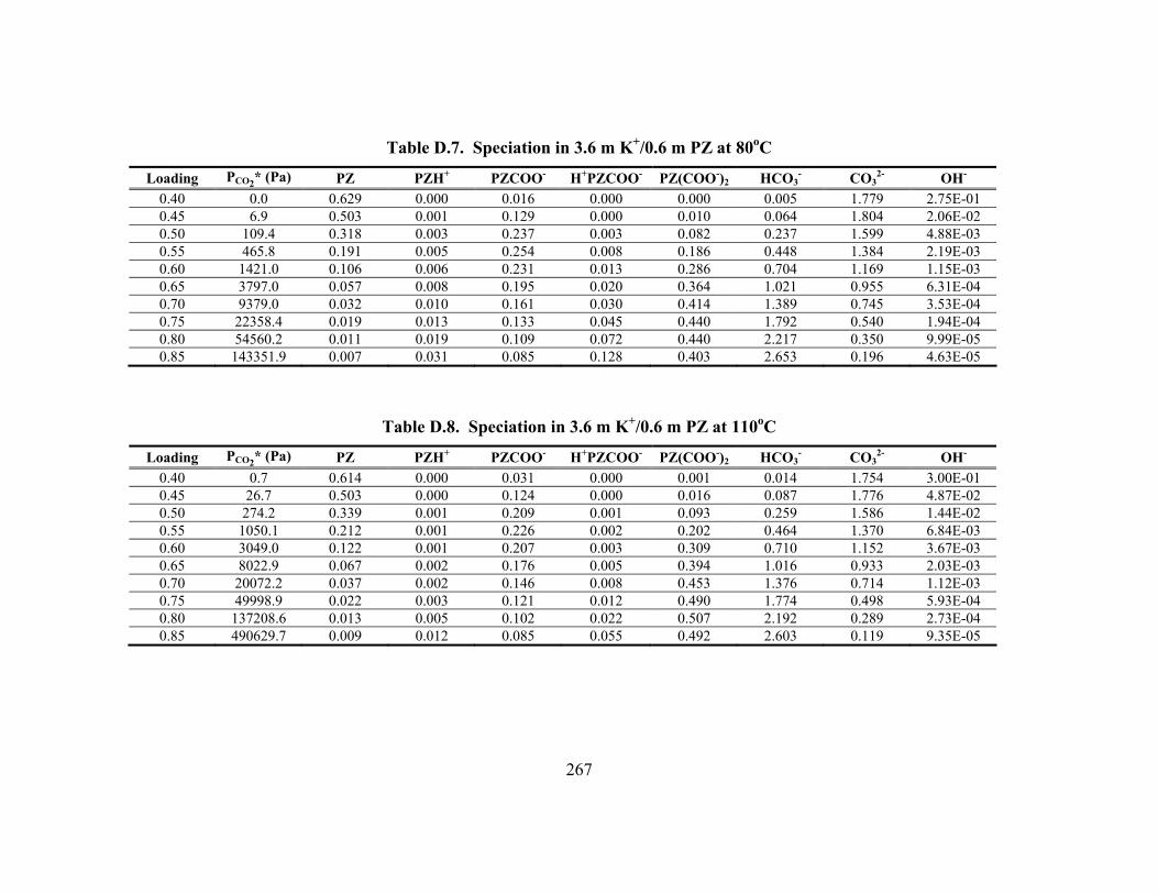
267
Table D.7. Speciation in 3.6 m K+/0.6 m PZ at 80oC
Loading PCO2* (Pa) PZ PZH+ PZCOO- H+PZCOO- PZ(COO-)2 HCO3- CO3
2- OH-
0.40 0.0 0.629 0.000 0.016 0.000 0.000 0.005 1.779 2.75E-01 0.45 6.9 0.503 0.001 0.129 0.000 0.010 0.064 1.804 2.06E-02 0.50 109.4 0.318 0.003 0.237 0.003 0.082 0.237 1.599 4.88E-03 0.55 465.8 0.191 0.005 0.254 0.008 0.186 0.448 1.384 2.19E-03 0.60 1421.0 0.106 0.006 0.231 0.013 0.286 0.704 1.169 1.15E-03 0.65 3797.0 0.057 0.008 0.195 0.020 0.364 1.021 0.955 6.31E-04 0.70 9379.0 0.032 0.010 0.161 0.030 0.414 1.389 0.745 3.53E-04 0.75 22358.4 0.019 0.013 0.133 0.045 0.440 1.792 0.540 1.94E-04 0.80 54560.2 0.011 0.019 0.109 0.072 0.440 2.217 0.350 9.99E-05 0.85 143351.9 0.007 0.031 0.085 0.128 0.403 2.653 0.196 4.63E-05
Table D.8. Speciation in 3.6 m K+/0.6 m PZ at 110oC
Loading PCO2* (Pa) PZ PZH+ PZCOO- H+PZCOO- PZ(COO-)2 HCO3- CO3
2- OH-
0.40 0.7 0.614 0.000 0.031 0.000 0.001 0.014 1.754 3.00E-01 0.45 26.7 0.503 0.000 0.124 0.000 0.016 0.087 1.776 4.87E-02 0.50 274.2 0.339 0.001 0.209 0.001 0.093 0.259 1.586 1.44E-02 0.55 1050.1 0.212 0.001 0.226 0.002 0.202 0.464 1.370 6.84E-03 0.60 3049.0 0.122 0.001 0.207 0.003 0.309 0.710 1.152 3.67E-03 0.65 8022.9 0.067 0.002 0.176 0.005 0.394 1.016 0.933 2.03E-03 0.70 20072.2 0.037 0.002 0.146 0.008 0.453 1.376 0.714 1.12E-03 0.75 49998.9 0.022 0.003 0.121 0.012 0.490 1.774 0.498 5.93E-04 0.80 137208.6 0.013 0.005 0.102 0.022 0.507 2.192 0.289 2.73E-04 0.85 490629.7 0.009 0.012 0.085 0.055 0.492 2.603 0.119 9.35E-05
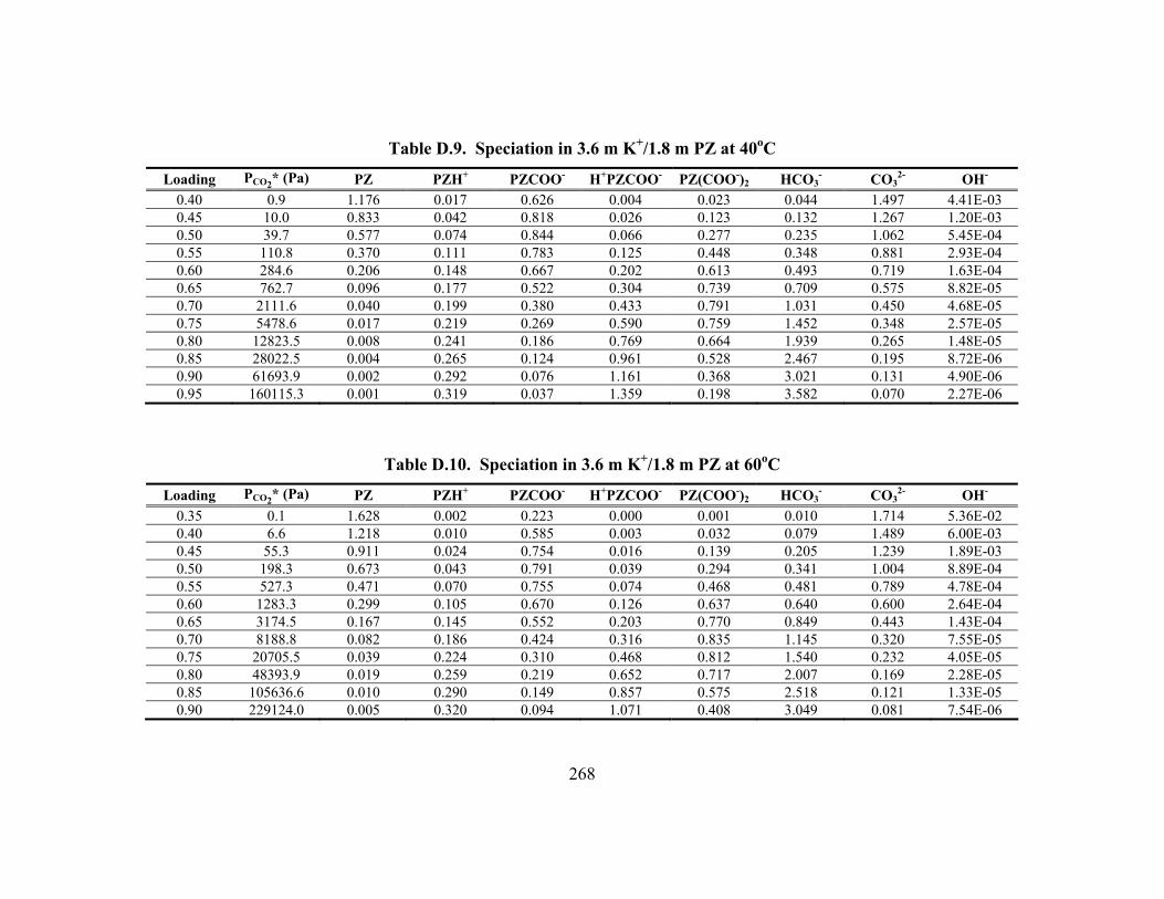
268
Table D.9. Speciation in 3.6 m K+/1.8 m PZ at 40oC
Loading PCO2* (Pa) PZ PZH+ PZCOO- H+PZCOO- PZ(COO-)2 HCO3- CO3
2- OH-
0.40 0.9 1.176 0.017 0.626 0.004 0.023 0.044 1.497 4.41E-03 0.45 10.0 0.833 0.042 0.818 0.026 0.123 0.132 1.267 1.20E-03 0.50 39.7 0.577 0.074 0.844 0.066 0.277 0.235 1.062 5.45E-04 0.55 110.8 0.370 0.111 0.783 0.125 0.448 0.348 0.881 2.93E-04 0.60 284.6 0.206 0.148 0.667 0.202 0.613 0.493 0.719 1.63E-04 0.65 762.7 0.096 0.177 0.522 0.304 0.739 0.709 0.575 8.82E-05 0.70 2111.6 0.040 0.199 0.380 0.433 0.791 1.031 0.450 4.68E-05 0.75 5478.6 0.017 0.219 0.269 0.590 0.759 1.452 0.348 2.57E-05 0.80 12823.5 0.008 0.241 0.186 0.769 0.664 1.939 0.265 1.48E-05 0.85 28022.5 0.004 0.265 0.124 0.961 0.528 2.467 0.195 8.72E-06 0.90 61693.9 0.002 0.292 0.076 1.161 0.368 3.021 0.131 4.90E-06 0.95 160115.3 0.001 0.319 0.037 1.359 0.198 3.582 0.070 2.27E-06
Table D.10. Speciation in 3.6 m K+/1.8 m PZ at 60oC
Loading PCO2* (Pa) PZ PZH+ PZCOO- H+PZCOO- PZ(COO-)2 HCO3- CO3
2- OH-
0.35 0.1 1.628 0.002 0.223 0.000 0.001 0.010 1.714 5.36E-02 0.40 6.6 1.218 0.010 0.585 0.003 0.032 0.079 1.489 6.00E-03 0.45 55.3 0.911 0.024 0.754 0.016 0.139 0.205 1.239 1.89E-03 0.50 198.3 0.673 0.043 0.791 0.039 0.294 0.341 1.004 8.89E-04 0.55 527.3 0.471 0.070 0.755 0.074 0.468 0.481 0.789 4.78E-04 0.60 1283.3 0.299 0.105 0.670 0.126 0.637 0.640 0.600 2.64E-04 0.65 3174.5 0.167 0.145 0.552 0.203 0.770 0.849 0.443 1.43E-04 0.70 8188.8 0.082 0.186 0.424 0.316 0.835 1.145 0.320 7.55E-05 0.75 20705.5 0.039 0.224 0.310 0.468 0.812 1.540 0.232 4.05E-05 0.80 48393.9 0.019 0.259 0.219 0.652 0.717 2.007 0.169 2.28E-05 0.85 105636.6 0.010 0.290 0.149 0.857 0.575 2.518 0.121 1.33E-05 0.90 229124.0 0.005 0.320 0.094 1.071 0.408 3.049 0.081 7.54E-06
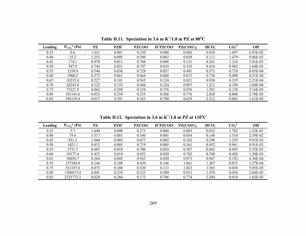
269
Table D.11. Speciation in 3.6 m K+/1.8 m PZ at 80oC
Loading PCO2* (Pa) PZ PZH+ PZCOO- H+PZCOO- PZ(COO-)2 HCO3- CO3
2- OH-
0.35 0.6 1.621 0.001 0.230 0.000 0.002 0.018 1.697 6.93E-02 0.40 25.2 1.253 0.005 0.549 0.002 0.039 0.111 1.479 9.86E-03 0.45 174.1 0.970 0.011 0.704 0.008 0.151 0.261 1.218 3.41E-03 0.50 587.9 0.744 0.021 0.747 0.019 0.310 0.416 0.962 1.64E-03 0.55 1554.9 0.546 0.036 0.728 0.037 0.491 0.571 0.718 8.65E-04 0.60 3900.5 0.372 0.061 0.664 0.068 0.672 0.736 0.498 4.51E-04 0.65 10232.4 0.227 0.101 0.565 0.124 0.821 0.936 0.319 2.21E-04 0.70 28243.8 0.122 0.155 0.444 0.224 0.897 1.211 0.198 1.04E-04 0.75 75327.9 0.062 0.209 0.328 0.376 0.876 1.582 0.128 5.16E-05 0.80 181141.6 0.032 0.254 0.235 0.568 0.776 2.028 0.088 2.78E-05 0.85 396139.4 0.017 0.291 0.163 0.780 0.629 2.512 0.062 1.61E-05
Table D.12. Speciation in 3.6 m K+/1.8 m PZ at 110oC
Loading PCO2* (Pa) PZ PZH+ PZCOO- H+PZCOO- PZ(COO-)2 HCO3- CO3
2- OH-
0.35 3.7 1.640 0.000 0.273 0.000 0.005 0.032 1.702 1.25E-01 0.40 79.6 1.317 0.001 0.540 0.001 0.054 0.140 1.510 2.59E-02 0.45 451.2 1.044 0.003 0.677 0.002 0.182 0.296 1.239 9.91E-03 0.50 1421.1 0.813 0.005 0.719 0.005 0.361 0.452 0.961 4.91E-03 0.55 3731.7 0.607 0.010 0.706 0.010 0.567 0.603 0.685 2.55E-03 0.60 10177.4 0.423 0.019 0.652 0.020 0.782 0.760 0.420 1.20E-03 0.65 36056.7 0.264 0.045 0.563 0.050 0.973 0.947 0.192 4.30E-04 0.70 157384.9 0.144 0.109 0.439 0.146 1.061 1.207 0.073 1.27E-04 0.75 521187.6 0.075 0.180 0.320 0.313 1.023 1.565 0.038 5.05E-05 0.80 1306073.9 0.041 0.229 0.233 0.509 0.912 1.976 0.024 2.64E-05 0.85 2725772.3 0.024 0.260 0.173 0.706 0.774 2.384 0.018 1.62E-05
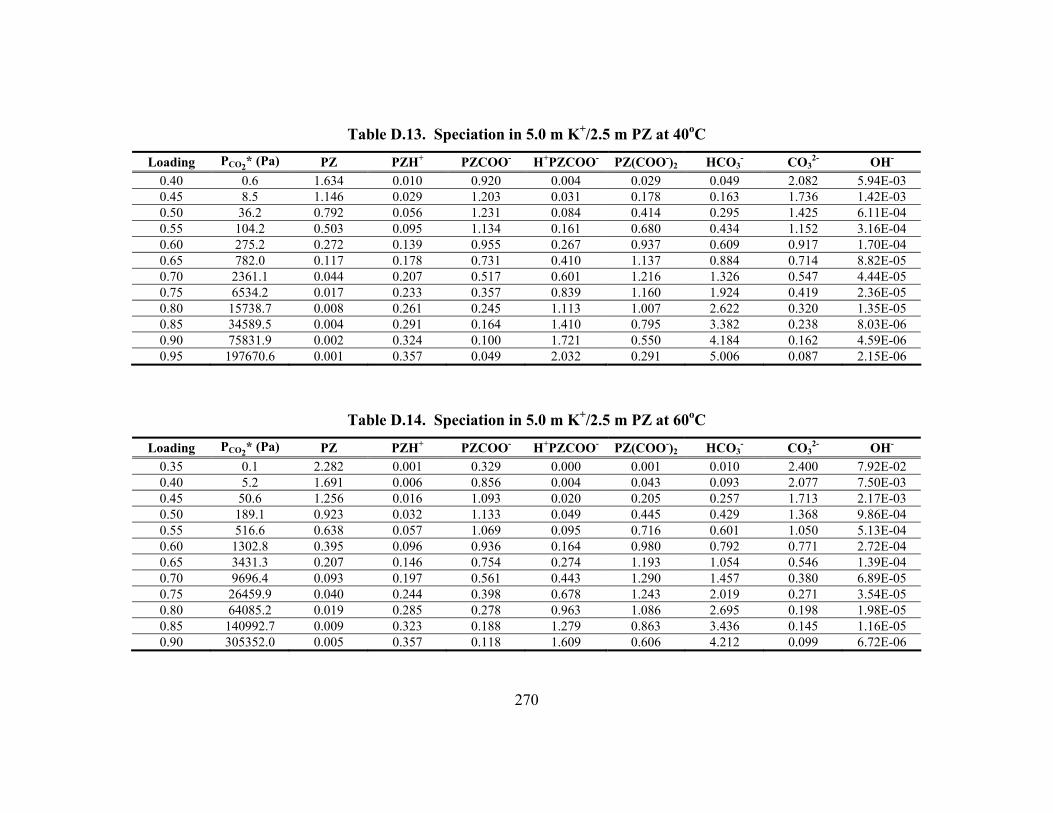
270
Table D.13. Speciation in 5.0 m K+/2.5 m PZ at 40oC
Loading PCO2* (Pa) PZ PZH+ PZCOO- H+PZCOO- PZ(COO-)2 HCO3- CO3
2- OH-
0.40 0.6 1.634 0.010 0.920 0.004 0.029 0.049 2.082 5.94E-03 0.45 8.5 1.146 0.029 1.203 0.031 0.178 0.163 1.736 1.42E-03 0.50 36.2 0.792 0.056 1.231 0.084 0.414 0.295 1.425 6.11E-04 0.55 104.2 0.503 0.095 1.134 0.161 0.680 0.434 1.152 3.16E-04 0.60 275.2 0.272 0.139 0.955 0.267 0.937 0.609 0.917 1.70E-04 0.65 782.0 0.117 0.178 0.731 0.410 1.137 0.884 0.714 8.82E-05 0.70 2361.1 0.044 0.207 0.517 0.601 1.216 1.326 0.547 4.44E-05 0.75 6534.2 0.017 0.233 0.357 0.839 1.160 1.924 0.419 2.36E-05 0.80 15738.7 0.008 0.261 0.245 1.113 1.007 2.622 0.320 1.35E-05 0.85 34589.5 0.004 0.291 0.164 1.410 0.795 3.382 0.238 8.03E-06 0.90 75831.9 0.002 0.324 0.100 1.721 0.550 4.184 0.162 4.59E-06 0.95 197670.6 0.001 0.357 0.049 2.032 0.291 5.006 0.087 2.15E-06
Table D.14. Speciation in 5.0 m K+/2.5 m PZ at 60oC
Loading PCO2* (Pa) PZ PZH+ PZCOO- H+PZCOO- PZ(COO-)2 HCO3- CO3
2- OH-
0.35 0.1 2.282 0.001 0.329 0.000 0.001 0.010 2.400 7.92E-02 0.40 5.2 1.691 0.006 0.856 0.004 0.043 0.093 2.077 7.50E-03 0.45 50.6 1.256 0.016 1.093 0.020 0.205 0.257 1.713 2.17E-03 0.50 189.1 0.923 0.032 1.133 0.049 0.445 0.429 1.368 9.86E-04 0.55 516.6 0.638 0.057 1.069 0.095 0.716 0.601 1.050 5.13E-04 0.60 1302.8 0.395 0.096 0.936 0.164 0.980 0.792 0.771 2.72E-04 0.65 3431.3 0.207 0.146 0.754 0.274 1.193 1.054 0.546 1.39E-04 0.70 9696.4 0.093 0.197 0.561 0.443 1.290 1.457 0.380 6.89E-05 0.75 26459.9 0.040 0.244 0.398 0.678 1.243 2.019 0.271 3.54E-05 0.80 64085.2 0.019 0.285 0.278 0.963 1.086 2.695 0.198 1.98E-05 0.85 140992.7 0.009 0.323 0.188 1.279 0.863 3.436 0.145 1.16E-05 0.90 305352.0 0.005 0.357 0.118 1.609 0.606 4.212 0.099 6.72E-06
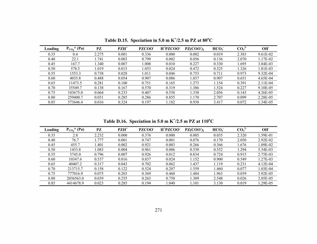
271
Table D.15. Speciation in 5.0 m K+/2.5 m PZ at 80oC
Loading PCO2* (Pa) PZ PZH+ PZCOO- H+PZCOO- PZ(COO-)2 HCO3- CO3
2- OH-
0.35 0.4 2.275 0.001 0.336 0.000 0.002 0.019 2.383 9.61E-02 0.40 22.1 1.741 0.003 0.799 0.002 0.056 0.136 2.070 1.17E-02 0.45 167.7 1.340 0.007 1.008 0.010 0.227 0.330 1.695 3.84E-03 0.50 578.5 1.019 0.015 1.053 0.024 0.472 0.525 1.326 1.81E-03 0.55 1553.3 0.738 0.028 1.011 0.046 0.753 0.711 0.973 9.32E-04 0.60 4035.8 0.488 0.054 0.907 0.086 1.037 0.907 0.651 4.65E-04 0.65 11473.5 0.281 0.100 0.751 0.165 1.273 1.154 0.391 2.11E-04 0.70 35549.7 0.138 0.167 0.570 0.319 1.386 1.524 0.227 9.10E-05 0.75 103675.0 0.064 0.233 0.407 0.558 1.338 2.056 0.143 4.26E-05 0.80 259400.7 0.031 0.285 0.286 0.855 1.170 2.707 0.099 2.28E-05 0.85 573646.4 0.016 0.324 0.197 1.182 0.938 3.417 0.072 1.34E-05
Table D.16. Speciation in 5.0 m K+/2.5 m PZ at 110oC
Loading PCO2* (Pa) PZ PZH+ PZCOO- H+PZCOO- PZ(COO-)2 HCO3- CO3
2- OH-
0.35 2.8 2.232 0.000 0.376 0.000 0.005 0.035 2.320 1.59E-01 0.40 76.7 1.777 0.001 0.747 0.001 0.076 0.170 2.050 2.92E-02 0.45 455.7 1.401 0.002 0.921 0.003 0.266 0.366 1.676 1.09E-02 0.50 1433.8 1.083 0.004 0.961 0.006 0.530 0.552 1.294 5.34E-03 0.55 3745.0 0.796 0.007 0.926 0.012 0.834 0.724 0.915 2.75E-03 0.60 10347.6 0.537 0.016 0.837 0.024 1.152 0.900 0.549 1.27E-03 0.65 40407.2 0.317 0.043 0.702 0.062 1.437 1.119 0.231 4.12E-04 0.70 213715.7 0.158 0.122 0.524 0.207 1.559 1.460 0.077 1.03E-04 0.75 777016.9 0.075 0.203 0.369 0.460 1.484 1.963 0.039 3.92E-05 0.80 2036563.0 0.039 0.255 0.263 0.750 1.309 2.548 0.026 2.05E-05 0.85 4414678.9 0.023 0.285 0.194 1.040 1.101 3.130 0.019 1.29E-05
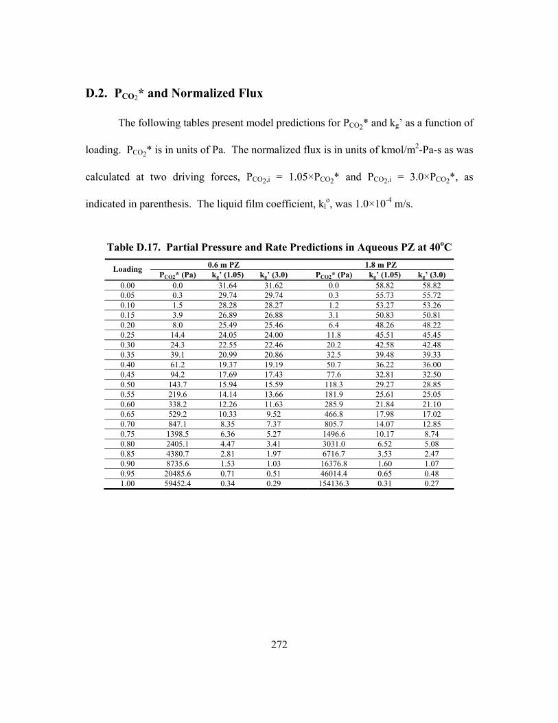
272
D.2. PCO2* and Normalized Flux
The following tables present model predictions for PCO2* and kg� as a function of
loading. PCO2* is in units of Pa. The normalized flux is in units of kmol/m2-Pa-s as was
calculated at two driving forces, PCO2,i = 1.05×PCO2* and PCO2,i = 3.0×PCO2*, as
indicated in parenthesis. The liquid film coefficient, klo, was 1.0×10⁻⁴ m/s.
Table D.17. Partial Pressure and Rate Predictions in Aqueous PZ at 40oC 0.6 m PZ 1.8 m PZ Loading
PCO2* (Pa) kg� (1.05) kg� (3.0) PCO2* (Pa) kg� (1.05) kg� (3.0) 0.00 0.0 31.64 31.62 0.0 58.82 58.82 0.05 0.3 29.74 29.74 0.3 55.73 55.72 0.10 1.5 28.28 28.27 1.2 53.27 53.26 0.15 3.9 26.89 26.88 3.1 50.83 50.81 0.20 8.0 25.49 25.46 6.4 48.26 48.22 0.25 14.4 24.05 24.00 11.8 45.51 45.45 0.30 24.3 22.55 22.46 20.2 42.58 42.48 0.35 39.1 20.99 20.86 32.5 39.48 39.33 0.40 61.2 19.37 19.19 50.7 36.22 36.00 0.45 94.2 17.69 17.43 77.6 32.81 32.50 0.50 143.7 15.94 15.59 118.3 29.27 28.85 0.55 219.6 14.14 13.66 181.9 25.61 25.05 0.60 338.2 12.26 11.63 285.9 21.84 21.10 0.65 529.2 10.33 9.52 466.8 17.98 17.02 0.70 847.1 8.35 7.37 805.7 14.07 12.85 0.75 1398.5 6.36 5.27 1496.6 10.17 8.74 0.80 2405.1 4.47 3.41 3031.0 6.52 5.08 0.85 4380.7 2.81 1.97 6716.7 3.53 2.47 0.90 8735.6 1.53 1.03 16376.8 1.60 1.07 0.95 20485.6 0.71 0.51 46014.4 0.65 0.48 1.00 59452.4 0.34 0.29 154136.3 0.31 0.27
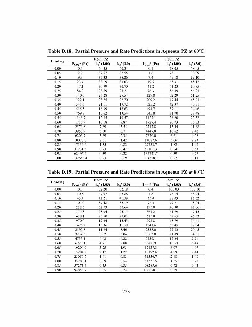
273
Table D.18. Partial Pressure and Rate Predictions in Aqueous PZ at 60oC 0.6 m PZ 1.8 m PZ Loading
PCO2* (Pa) kg� (1.05) kg� (3.0) PCO2* (Pa) kg� (1.05) kg� (3.0) 0.00 0.1 40.35 40.34 0.1 78.05 78.05 0.05 2.2 37.57 37.55 1.6 73.11 73.09 0.10 9.3 35.33 35.26 7.4 69.18 69.10 0.15 23.4 33.19 33.03 19.5 65.31 65.12 0.20 47.1 30.99 30.70 41.2 61.23 60.85 0.25 84.2 28.69 28.21 76.3 56.89 56.23 0.30 140.0 26.28 25.54 129.8 52.29 51.25 0.35 222.1 23.75 22.70 209.2 47.44 45.93 0.40 341.6 21.11 19.72 325.2 42.37 40.31 0.45 515.5 18.39 16.63 494.7 37.11 34.46 0.50 769.8 15.62 13.54 745.8 31.70 28.48 0.55 1145.7 12.85 10.57 1127.1 26.20 22.52 0.60 1710.9 10.18 7.87 1727.4 20.73 16.83 0.65 2579.8 7.69 5.55 2717.8 15.44 11.68 0.70 3953.9 5.50 3.71 4447.8 10.62 7.42 0.75 6205.7 3.69 2.35 7670.0 6.61 4.26 0.80 10070.6 2.31 1.42 14087.6 3.66 2.23 0.85 17134.4 1.35 0.82 27753.7 1.82 1.09 0.90 31231.5 0.73 0.47 59101.3 0.84 0.53 0.95 62496.4 0.39 0.28 137741.7 0.39 0.27 1.00 132683.4 0.23 0.19 334328.1 0.22 0.18
Table D.19. Partial Pressure and Rate Predictions in Aqueous PZ at 80oC 0.6 m PZ 1.8 m PZ Loading
PCO2* (Pa) kg� (1.05) kg� (3.0) PCO2* (Pa) kg� (1.05) kg� (3.0) 0.00 0.7 52.20 52.18 0.4 105.03 105.00 0.05 10.5 47.07 46.88 7.8 96.14 95.94 0.10 43.4 42.21 41.59 35.0 88.03 87.32 0.15 107.0 37.48 36.19 92.5 79.71 78.04 0.20 212.6 32.73 30.64 195.0 70.90 67.86 0.25 375.8 28.04 25.15 361.2 61.79 57.15 0.30 618.1 23.50 20.01 615.8 52.65 46.53 0.35 970.0 19.24 15.43 992.8 43.79 36.61 0.40 1475.2 15.36 11.58 1541.6 35.45 27.84 0.45 2197.8 11.94 8.46 2338.0 27.83 20.45 0.50 3234.3 9.02 6.04 3503.0 21.09 14.51 0.55 4733.1 6.62 4.22 5239.1 15.34 9.91 0.60 6929.1 4.71 2.88 7900.9 10.63 6.49 0.65 10204.9 3.25 1.93 12137.3 6.97 4.07 0.70 15204.2 2.17 1.27 19192.6 4.29 2.44 0.75 23050.7 1.41 0.83 31550.7 2.48 1.40 0.80 35788.1 0.89 0.54 54331.5 1.35 0.78 0.85 57275.6 0.55 0.35 98285.6 0.72 0.44 0.90 94853.7 0.35 0.24 185870.3 0.39 0.26
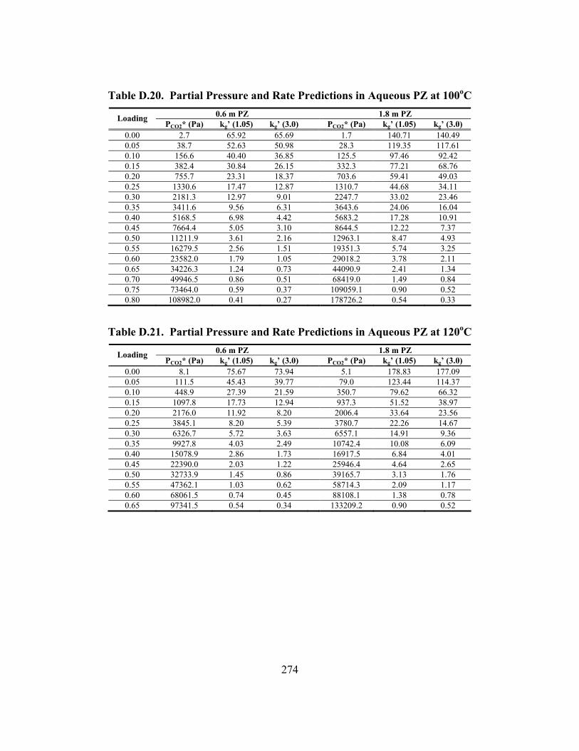
274
Table D.20. Partial Pressure and Rate Predictions in Aqueous PZ at 100oC 0.6 m PZ 1.8 m PZ Loading
PCO2* (Pa) kg� (1.05) kg� (3.0) PCO2* (Pa) kg� (1.05) kg� (3.0) 0.00 2.7 65.92 65.69 1.7 140.71 140.49 0.05 38.7 52.63 50.98 28.3 119.35 117.61 0.10 156.6 40.40 36.85 125.5 97.46 92.42 0.15 382.4 30.84 26.15 332.3 77.21 68.76 0.20 755.7 23.31 18.37 703.6 59.41 49.03 0.25 1330.6 17.47 12.87 1310.7 44.68 34.11 0.30 2181.3 12.97 9.01 2247.7 33.02 23.46 0.35 3411.6 9.56 6.31 3643.6 24.06 16.04 0.40 5168.5 6.98 4.42 5683.2 17.28 10.91 0.45 7664.4 5.05 3.10 8644.5 12.22 7.37 0.50 11211.9 3.61 2.16 12963.1 8.47 4.93 0.55 16279.5 2.56 1.51 19351.3 5.74 3.25 0.60 23582.0 1.79 1.05 29018.2 3.78 2.11 0.65 34226.3 1.24 0.73 44090.9 2.41 1.34 0.70 49946.5 0.86 0.51 68419.0 1.49 0.84 0.75 73464.0 0.59 0.37 109059.1 0.90 0.52 0.80 108982.0 0.41 0.27 178726.2 0.54 0.33
Table D.21. Partial Pressure and Rate Predictions in Aqueous PZ at 120oC 0.6 m PZ 1.8 m PZ Loading
PCO2* (Pa) kg� (1.05) kg� (3.0) PCO2* (Pa) kg� (1.05) kg� (3.0) 0.00 8.1 75.67 73.94 5.1 178.83 177.09 0.05 111.5 45.43 39.77 79.0 123.44 114.37 0.10 448.9 27.39 21.59 350.7 79.62 66.32 0.15 1097.8 17.73 12.94 937.3 51.52 38.97 0.20 2176.0 11.92 8.20 2006.4 33.64 23.56 0.25 3845.1 8.20 5.39 3780.7 22.26 14.67 0.30 6326.7 5.72 3.63 6557.1 14.91 9.36 0.35 9927.8 4.03 2.49 10742.4 10.08 6.09 0.40 15078.9 2.86 1.73 16917.5 6.84 4.01 0.45 22390.0 2.03 1.22 25946.4 4.64 2.65 0.50 32733.9 1.45 0.86 39165.7 3.13 1.76 0.55 47362.1 1.03 0.62 58714.3 2.09 1.17 0.60 68061.5 0.74 0.45 88108.1 1.38 0.78 0.65 97341.5 0.54 0.34 133209.2 0.90 0.52
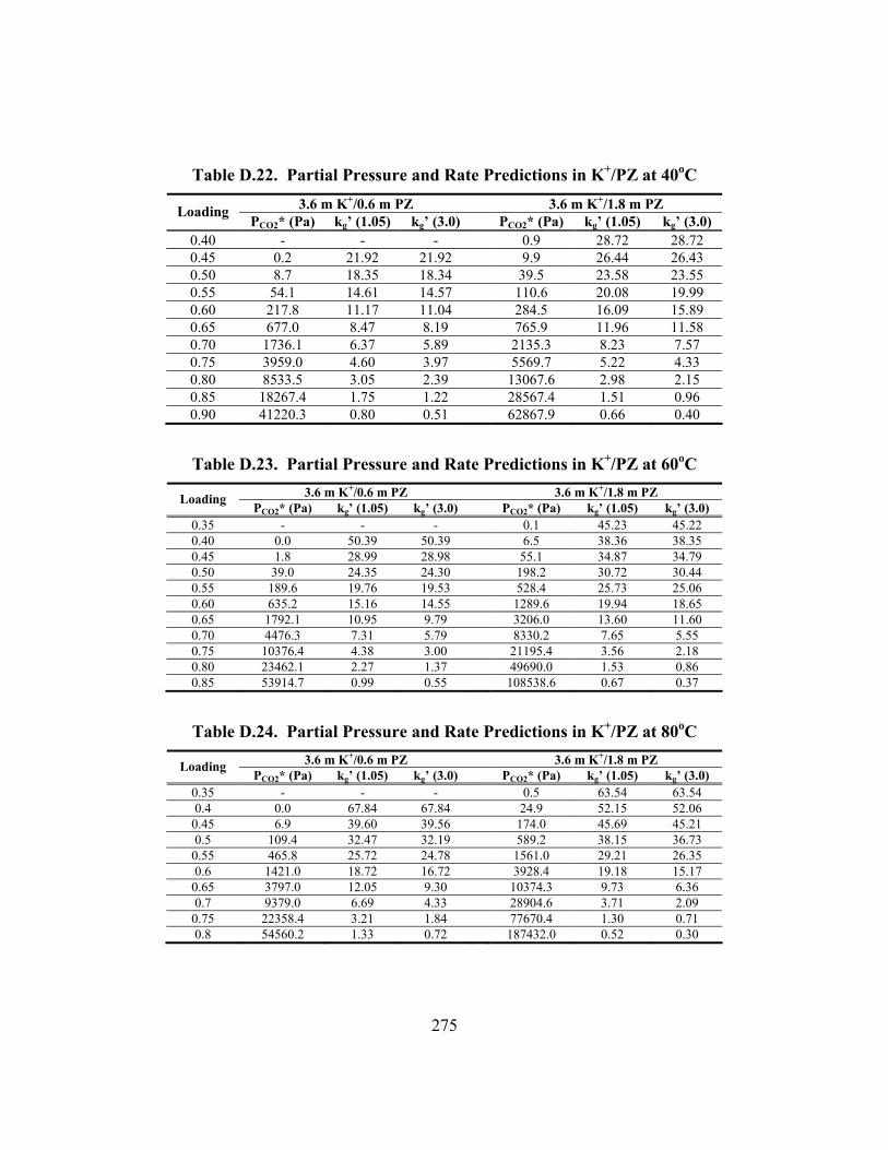
275
Table D.22. Partial Pressure and Rate Predictions in K+/PZ at 40oC 3.6 m K+/0.6 m PZ 3.6 m K+/1.8 m PZ Loading
PCO2* (Pa) kg� (1.05) kg� (3.0) PCO2* (Pa) kg� (1.05) kg� (3.0) 0.40 - - - 0.9 28.72 28.72 0.45 0.2 21.92 21.92 9.9 26.44 26.43 0.50 8.7 18.35 18.34 39.5 23.58 23.55 0.55 54.1 14.61 14.57 110.6 20.08 19.99 0.60 217.8 11.17 11.04 284.5 16.09 15.89 0.65 677.0 8.47 8.19 765.9 11.96 11.58 0.70 1736.1 6.37 5.89 2135.3 8.23 7.57 0.75 3959.0 4.60 3.97 5569.7 5.22 4.33 0.80 8533.5 3.05 2.39 13067.6 2.98 2.15 0.85 18267.4 1.75 1.22 28567.4 1.51 0.96 0.90 41220.3 0.80 0.51 62867.9 0.66 0.40
Table D.23. Partial Pressure and Rate Predictions in K+/PZ at 60oC 3.6 m K+/0.6 m PZ 3.6 m K+/1.8 m PZ Loading
PCO2* (Pa) kg� (1.05) kg� (3.0) PCO2* (Pa) kg� (1.05) kg� (3.0) 0.35 - - - 0.1 45.23 45.22 0.40 0.0 50.39 50.39 6.5 38.36 38.35 0.45 1.8 28.99 28.98 55.1 34.87 34.79 0.50 39.0 24.35 24.30 198.2 30.72 30.44 0.55 189.6 19.76 19.53 528.4 25.73 25.06 0.60 635.2 15.16 14.55 1289.6 19.94 18.65 0.65 1792.1 10.95 9.79 3206.0 13.60 11.60 0.70 4476.3 7.31 5.79 8330.2 7.65 5.55 0.75 10376.4 4.38 3.00 21195.4 3.56 2.18 0.80 23462.1 2.27 1.37 49690.0 1.53 0.86 0.85 53914.7 0.99 0.55 108538.6 0.67 0.37
Table D.24. Partial Pressure and Rate Predictions in K+/PZ at 80oC 3.6 m K+/0.6 m PZ 3.6 m K+/1.8 m PZ Loading
PCO2* (Pa) kg� (1.05) kg� (3.0) PCO2* (Pa) kg� (1.05) kg� (3.0) 0.35 - - - 0.5 63.54 63.54 0.4 0.0 67.84 67.84 24.9 52.15 52.06
0.45 6.9 39.60 39.56 174.0 45.69 45.21 0.5 109.4 32.47 32.19 589.2 38.15 36.73
0.55 465.8 25.72 24.78 1561.0 29.21 26.35 0.6 1421.0 18.72 16.72 3928.4 19.18 15.17
0.65 3797.0 12.05 9.30 10374.3 9.73 6.36 0.7 9379.0 6.69 4.33 28904.6 3.71 2.09
0.75 22358.4 3.21 1.84 77670.4 1.30 0.71 0.8 54560.2 1.33 0.72 187432.0 0.52 0.30
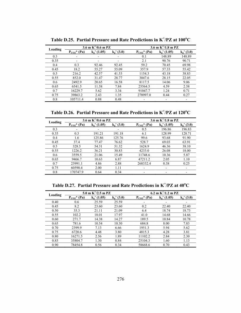
276
Table D.25. Partial Pressure and Rate Predictions in K+/PZ at 100oC 3.6 m K+/0.6 m PZ 3.6 m K+/1.8 m PZ Loading
PCO2* (Pa) kg� (1.05) kg� (3.0) PCO2* (Pa) kg� (1.05) kg� (3.0) 0.3 - - - 0.1 148.89 148.89
0.35 - - - 2.1 90.76 90.71 0.4 0.3 92.46 92.45 59.2 70.45 69.98
0.45 18.2 55.27 55.09 357.9 57.33 55.42 0.5 216.2 42.57 41.53 1154.3 43.18 38.83
0.55 852.0 31.47 28.77 3047.6 28.15 22.05 0.6 2492.9 20.65 16.58 8117.5 14.06 9.06
0.65 6541.5 11.58 7.84 25564.5 4.59 2.58 0.7 16229.7 5.62 3.34 91047.7 1.24 0.71
0.75 39863.2 2.43 1.35 278997.0 0.44 0.27 0.8 105711.4 0.88 0.48 - - -
Table D.26. Partial Pressure and Rate Predictions in K+/PZ at 120oC 3.6 m K+/0.6 m PZ 3.6 m K+/1.8 m PZ Loading
PCO2* (Pa) kg� (1.05) kg� (3.0) PCO2* (Pa) kg� (1.05) kg� (3.0) 0.3 - - - 0.5 196.86 196.83
0.35 0.3 191.21 191.18 6.1 128.99 128.71 0.4 1.6 125.86 125.76 99.6 93.68 91.90
0.45 37.4 77.47 76.62 528.7 69.03 63.91 0.5 328.5 54.31 51.32 1624.9 46.36 38.10
0.55 1226.2 36.21 30.83 4233.0 26.08 18.00 0.6 3559.5 21.06 15.49 11748.6 10.36 5.87
0.65 9466.7 10.63 6.87 47211.2 2.05 1.10 0.7 23991.1 4.86 2.88 268332.4 0.38 0.25
0.75 60590.4 2.00 1.11 - - - 0.8 170747.9 0.64 0.34 - - -
Table D.27. Partial Pressure and Rate Predictions in K+/PZ at 40oC 5.0 m K+/2.5 m PZ 6.2 m K+/1.2 m PZ Loading
PCO2* (Pa) kg� (1.05) kg� (3.0) PCO2* (Pa) kg� (1.05) kg� (3.0) 0.40 0.6 25.59 25.59 - - - 0.45 8.2 23.60 23.60 0.2 22.40 22.40 0.50 35.3 21.11 21.09 6.4 18.74 18.73 0.55 102.2 18.01 17.97 41.0 14.68 14.66 0.60 271.7 14.38 14.27 189.5 10.84 10.78 0.65 781.6 10.54 10.30 684.8 8.00 7.83 0.70 2399.9 7.13 6.66 1951.3 5.94 5.62 0.75 6720.6 4.48 3.80 4815.3 4.28 3.81 0.80 16271.5 2.56 1.89 11102.2 2.84 2.30 0.85 35804.7 1.30 0.84 25104.3 1.60 1.13 0.90 78454.8 0.56 0.34 58668.6 0.70 0.43
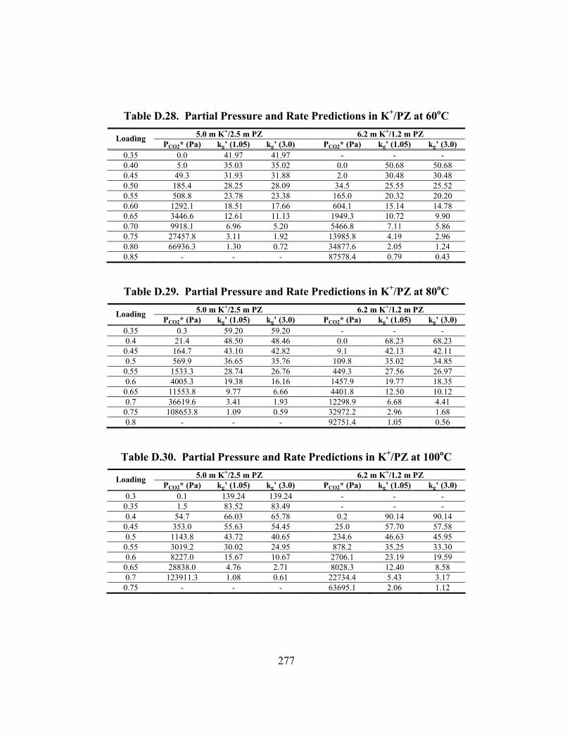
277
Table D.28. Partial Pressure and Rate Predictions in K+/PZ at 60oC 5.0 m K+/2.5 m PZ 6.2 m K+/1.2 m PZ Loading
PCO2* (Pa) kg� (1.05) kg� (3.0) PCO2* (Pa) kg� (1.05) kg� (3.0) 0.35 0.0 41.97 41.97 - - - 0.40 5.0 35.03 35.02 0.0 50.68 50.68 0.45 49.3 31.93 31.88 2.0 30.48 30.48 0.50 185.4 28.25 28.09 34.5 25.55 25.52 0.55 508.8 23.78 23.38 165.0 20.32 20.20 0.60 1292.1 18.51 17.66 604.1 15.14 14.78 0.65 3446.6 12.61 11.13 1949.3 10.72 9.90 0.70 9918.1 6.96 5.20 5466.8 7.11 5.86 0.75 27457.8 3.11 1.92 13985.8 4.19 2.96 0.80 66936.3 1.30 0.72 34877.6 2.05 1.24 0.85 - - - 87578.4 0.79 0.43
Table D.29. Partial Pressure and Rate Predictions in K+/PZ at 80oC 5.0 m K+/2.5 m PZ 6.2 m K+/1.2 m PZ Loading
PCO2* (Pa) kg� (1.05) kg� (3.0) PCO2* (Pa) kg� (1.05) kg� (3.0) 0.35 0.3 59.20 59.20 - - - 0.4 21.4 48.50 48.46 0.0 68.23 68.23
0.45 164.7 43.10 42.82 9.1 42.13 42.11 0.5 569.9 36.65 35.76 109.8 35.02 34.85
0.55 1533.3 28.74 26.76 449.3 27.56 26.97 0.6 4005.3 19.38 16.16 1457.9 19.77 18.35
0.65 11553.8 9.77 6.66 4401.8 12.50 10.12 0.7 36619.6 3.41 1.93 12298.9 6.68 4.41
0.75 108653.8 1.09 0.59 32972.2 2.96 1.68 0.8 - - - 92751.4 1.05 0.56
Table D.30. Partial Pressure and Rate Predictions in K+/PZ at 100oC 5.0 m K+/2.5 m PZ 6.2 m K+/1.2 m PZ Loading
PCO2* (Pa) kg� (1.05) kg� (3.0) PCO2* (Pa) kg� (1.05) kg� (3.0) 0.3 0.1 139.24 139.24 - - -
0.35 1.5 83.52 83.49 - - - 0.4 54.7 66.03 65.78 0.2 90.14 90.14
0.45 353.0 55.63 54.45 25.0 57.70 57.58 0.5 1143.8 43.72 40.65 234.6 46.63 45.95
0.55 3019.2 30.02 24.95 878.2 35.25 33.30 0.6 8227.0 15.67 10.67 2706.1 23.19 19.59
0.65 28838.0 4.76 2.71 8028.3 12.40 8.58 0.7 123911.3 1.08 0.61 22734.4 5.43 3.17
0.75 - - - 63695.1 2.06 1.12
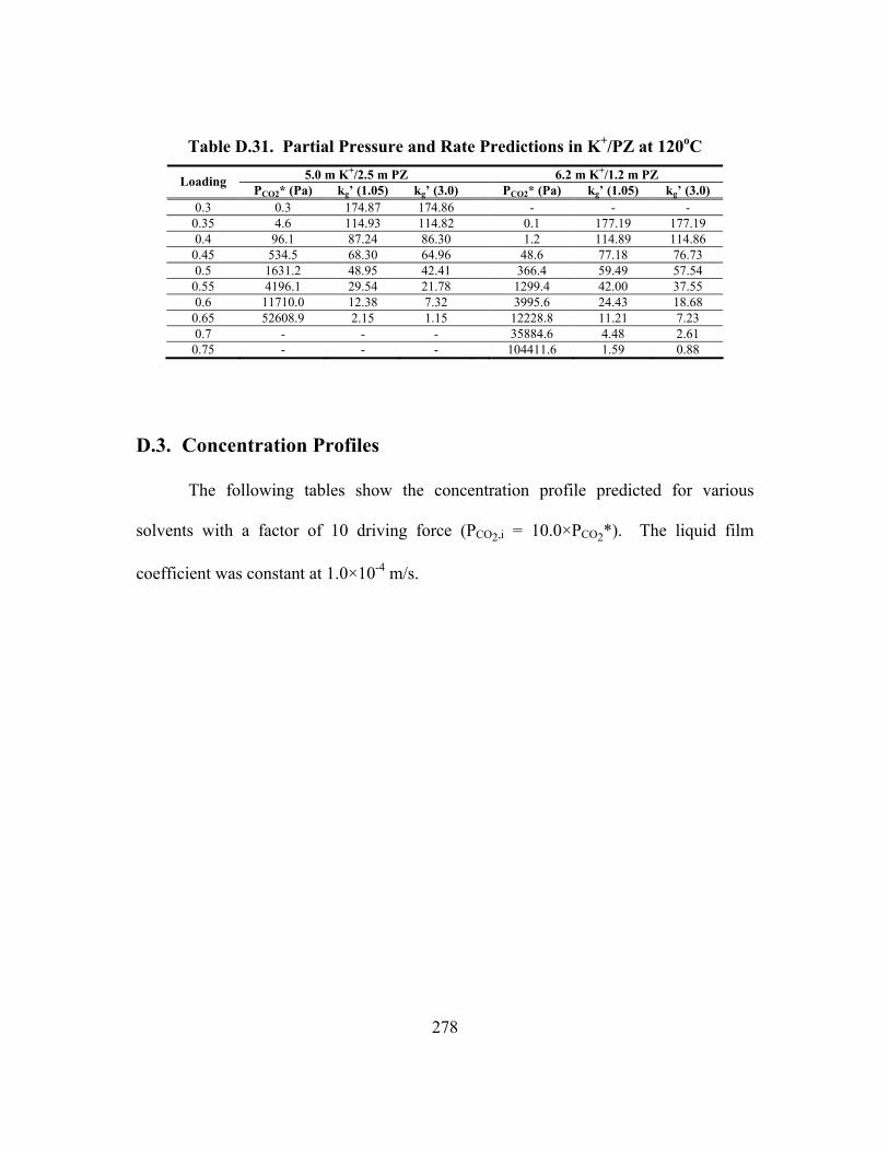
278
Table D.31. Partial Pressure and Rate Predictions in K+/PZ at 120oC 5.0 m K+/2.5 m PZ 6.2 m K+/1.2 m PZ Loading
PCO2* (Pa) kg� (1.05) kg� (3.0) PCO2* (Pa) kg� (1.05) kg� (3.0) 0.3 0.3 174.87 174.86 - - -
0.35 4.6 114.93 114.82 0.1 177.19 177.19 0.4 96.1 87.24 86.30 1.2 114.89 114.86
0.45 534.5 68.30 64.96 48.6 77.18 76.73 0.5 1631.2 48.95 42.41 366.4 59.49 57.54
0.55 4196.1 29.54 21.78 1299.4 42.00 37.55 0.6 11710.0 12.38 7.32 3995.6 24.43 18.68
0.65 52608.9 2.15 1.15 12228.8 11.21 7.23 0.7 - - - 35884.6 4.48 2.61
0.75 - - - 104411.6 1.59 0.88
D.3. Concentration Profiles
The following tables show the concentration profile predicted for various
solvents with a factor of 10 driving force (PCO2,i = 10.0×PCO2*). The liquid film
coefficient was constant at 1.0×10⁻⁴ m/s.
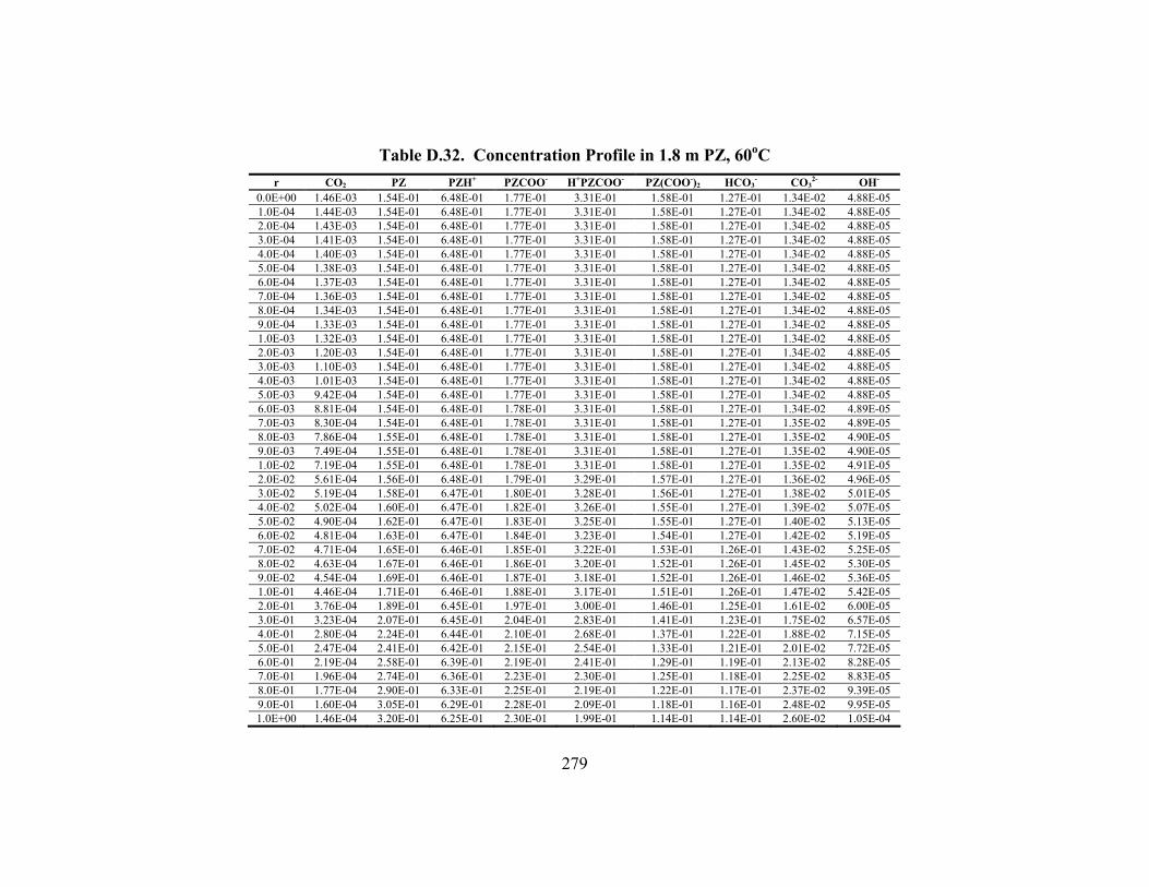
279
Table D.32. Concentration Profile in 1.8 m PZ, 60oC r CO2 PZ PZH+ PZCOO- H+PZCOO- PZ(COO-)2 HCO3
- CO32- OH-
0.0E+00 1.46E-03 1.54E-01 6.48E-01 1.77E-01 3.31E-01 1.58E-01 1.27E-01 1.34E-02 4.88E-05 1.0E-04 1.44E-03 1.54E-01 6.48E-01 1.77E-01 3.31E-01 1.58E-01 1.27E-01 1.34E-02 4.88E-05 2.0E-04 1.43E-03 1.54E-01 6.48E-01 1.77E-01 3.31E-01 1.58E-01 1.27E-01 1.34E-02 4.88E-05 3.0E-04 1.41E-03 1.54E-01 6.48E-01 1.77E-01 3.31E-01 1.58E-01 1.27E-01 1.34E-02 4.88E-05 4.0E-04 1.40E-03 1.54E-01 6.48E-01 1.77E-01 3.31E-01 1.58E-01 1.27E-01 1.34E-02 4.88E-05 5.0E-04 1.38E-03 1.54E-01 6.48E-01 1.77E-01 3.31E-01 1.58E-01 1.27E-01 1.34E-02 4.88E-05 6.0E-04 1.37E-03 1.54E-01 6.48E-01 1.77E-01 3.31E-01 1.58E-01 1.27E-01 1.34E-02 4.88E-05 7.0E-04 1.36E-03 1.54E-01 6.48E-01 1.77E-01 3.31E-01 1.58E-01 1.27E-01 1.34E-02 4.88E-05 8.0E-04 1.34E-03 1.54E-01 6.48E-01 1.77E-01 3.31E-01 1.58E-01 1.27E-01 1.34E-02 4.88E-05 9.0E-04 1.33E-03 1.54E-01 6.48E-01 1.77E-01 3.31E-01 1.58E-01 1.27E-01 1.34E-02 4.88E-05 1.0E-03 1.32E-03 1.54E-01 6.48E-01 1.77E-01 3.31E-01 1.58E-01 1.27E-01 1.34E-02 4.88E-05 2.0E-03 1.20E-03 1.54E-01 6.48E-01 1.77E-01 3.31E-01 1.58E-01 1.27E-01 1.34E-02 4.88E-05 3.0E-03 1.10E-03 1.54E-01 6.48E-01 1.77E-01 3.31E-01 1.58E-01 1.27E-01 1.34E-02 4.88E-05 4.0E-03 1.01E-03 1.54E-01 6.48E-01 1.77E-01 3.31E-01 1.58E-01 1.27E-01 1.34E-02 4.88E-05 5.0E-03 9.42E-04 1.54E-01 6.48E-01 1.77E-01 3.31E-01 1.58E-01 1.27E-01 1.34E-02 4.88E-05 6.0E-03 8.81E-04 1.54E-01 6.48E-01 1.78E-01 3.31E-01 1.58E-01 1.27E-01 1.34E-02 4.89E-05 7.0E-03 8.30E-04 1.54E-01 6.48E-01 1.78E-01 3.31E-01 1.58E-01 1.27E-01 1.35E-02 4.89E-05 8.0E-03 7.86E-04 1.55E-01 6.48E-01 1.78E-01 3.31E-01 1.58E-01 1.27E-01 1.35E-02 4.90E-05 9.0E-03 7.49E-04 1.55E-01 6.48E-01 1.78E-01 3.31E-01 1.58E-01 1.27E-01 1.35E-02 4.90E-05 1.0E-02 7.19E-04 1.55E-01 6.48E-01 1.78E-01 3.31E-01 1.58E-01 1.27E-01 1.35E-02 4.91E-05 2.0E-02 5.61E-04 1.56E-01 6.48E-01 1.79E-01 3.29E-01 1.57E-01 1.27E-01 1.36E-02 4.96E-05 3.0E-02 5.19E-04 1.58E-01 6.47E-01 1.80E-01 3.28E-01 1.56E-01 1.27E-01 1.38E-02 5.01E-05 4.0E-02 5.02E-04 1.60E-01 6.47E-01 1.82E-01 3.26E-01 1.55E-01 1.27E-01 1.39E-02 5.07E-05 5.0E-02 4.90E-04 1.62E-01 6.47E-01 1.83E-01 3.25E-01 1.55E-01 1.27E-01 1.40E-02 5.13E-05 6.0E-02 4.81E-04 1.63E-01 6.47E-01 1.84E-01 3.23E-01 1.54E-01 1.27E-01 1.42E-02 5.19E-05 7.0E-02 4.71E-04 1.65E-01 6.46E-01 1.85E-01 3.22E-01 1.53E-01 1.26E-01 1.43E-02 5.25E-05 8.0E-02 4.63E-04 1.67E-01 6.46E-01 1.86E-01 3.20E-01 1.52E-01 1.26E-01 1.45E-02 5.30E-05 9.0E-02 4.54E-04 1.69E-01 6.46E-01 1.87E-01 3.18E-01 1.52E-01 1.26E-01 1.46E-02 5.36E-05 1.0E-01 4.46E-04 1.71E-01 6.46E-01 1.88E-01 3.17E-01 1.51E-01 1.26E-01 1.47E-02 5.42E-05 2.0E-01 3.76E-04 1.89E-01 6.45E-01 1.97E-01 3.00E-01 1.46E-01 1.25E-01 1.61E-02 6.00E-05 3.0E-01 3.23E-04 2.07E-01 6.45E-01 2.04E-01 2.83E-01 1.41E-01 1.23E-01 1.75E-02 6.57E-05 4.0E-01 2.80E-04 2.24E-01 6.44E-01 2.10E-01 2.68E-01 1.37E-01 1.22E-01 1.88E-02 7.15E-05 5.0E-01 2.47E-04 2.41E-01 6.42E-01 2.15E-01 2.54E-01 1.33E-01 1.21E-01 2.01E-02 7.72E-05 6.0E-01 2.19E-04 2.58E-01 6.39E-01 2.19E-01 2.41E-01 1.29E-01 1.19E-01 2.13E-02 8.28E-05 7.0E-01 1.96E-04 2.74E-01 6.36E-01 2.23E-01 2.30E-01 1.25E-01 1.18E-01 2.25E-02 8.83E-05 8.0E-01 1.77E-04 2.90E-01 6.33E-01 2.25E-01 2.19E-01 1.22E-01 1.17E-01 2.37E-02 9.39E-05 9.0E-01 1.60E-04 3.05E-01 6.29E-01 2.28E-01 2.09E-01 1.18E-01 1.16E-01 2.48E-02 9.95E-05 1.0E+00 1.46E-04 3.20E-01 6.25E-01 2.30E-01 1.99E-01 1.14E-01 1.14E-01 2.60E-02 1.05E-04
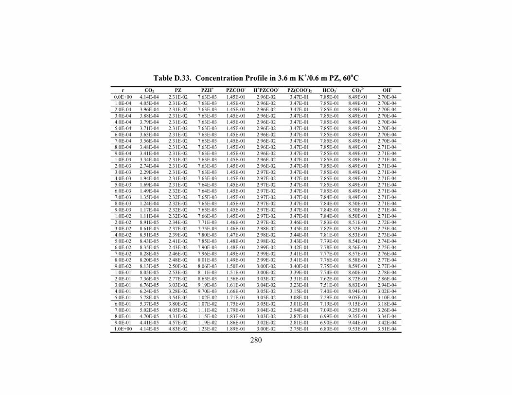
280
Table D.33. Concentration Profile in 3.6 m K+/0.6 m PZ, 60oC r CO2 PZ PZH+ PZCOO- H+PZCOO- PZ(COO-)2 HCO3
- CO32- OH-
0.0E+00 4.14E-04 2.31E-02 7.63E-03 1.45E-01 2.96E-02 3.47E-01 7.85E-01 8.49E-01 2.70E-04 1.0E-04 4.05E-04 2.31E-02 7.63E-03 1.45E-01 2.96E-02 3.47E-01 7.85E-01 8.49E-01 2.70E-04 2.0E-04 3.96E-04 2.31E-02 7.63E-03 1.45E-01 2.96E-02 3.47E-01 7.85E-01 8.49E-01 2.70E-04 3.0E-04 3.88E-04 2.31E-02 7.63E-03 1.45E-01 2.96E-02 3.47E-01 7.85E-01 8.49E-01 2.70E-04 4.0E-04 3.79E-04 2.31E-02 7.63E-03 1.45E-01 2.96E-02 3.47E-01 7.85E-01 8.49E-01 2.70E-04 5.0E-04 3.71E-04 2.31E-02 7.63E-03 1.45E-01 2.96E-02 3.47E-01 7.85E-01 8.49E-01 2.70E-04 6.0E-04 3.63E-04 2.31E-02 7.63E-03 1.45E-01 2.96E-02 3.47E-01 7.85E-01 8.49E-01 2.70E-04 7.0E-04 3.56E-04 2.31E-02 7.63E-03 1.45E-01 2.96E-02 3.47E-01 7.85E-01 8.49E-01 2.70E-04 8.0E-04 3.48E-04 2.31E-02 7.63E-03 1.45E-01 2.96E-02 3.47E-01 7.85E-01 8.49E-01 2.71E-04 9.0E-04 3.41E-04 2.31E-02 7.63E-03 1.45E-01 2.96E-02 3.47E-01 7.85E-01 8.49E-01 2.71E-04 1.0E-03 3.34E-04 2.31E-02 7.63E-03 1.45E-01 2.96E-02 3.47E-01 7.85E-01 8.49E-01 2.71E-04 2.0E-03 2.74E-04 2.31E-02 7.63E-03 1.45E-01 2.96E-02 3.47E-01 7.85E-01 8.49E-01 2.71E-04 3.0E-03 2.29E-04 2.31E-02 7.63E-03 1.45E-01 2.97E-02 3.47E-01 7.85E-01 8.49E-01 2.71E-04 4.0E-03 1.94E-04 2.31E-02 7.63E-03 1.45E-01 2.97E-02 3.47E-01 7.85E-01 8.49E-01 2.71E-04 5.0E-03 1.69E-04 2.31E-02 7.64E-03 1.45E-01 2.97E-02 3.47E-01 7.85E-01 8.49E-01 2.71E-04 6.0E-03 1.49E-04 2.32E-02 7.64E-03 1.45E-01 2.97E-02 3.47E-01 7.85E-01 8.49E-01 2.71E-04 7.0E-03 1.35E-04 2.32E-02 7.65E-03 1.45E-01 2.97E-02 3.47E-01 7.84E-01 8.49E-01 2.71E-04 8.0E-03 1.24E-04 2.32E-02 7.65E-03 1.45E-01 2.97E-02 3.47E-01 7.84E-01 8.50E-01 2.71E-04 9.0E-03 1.17E-04 2.32E-02 7.65E-03 1.45E-01 2.97E-02 3.47E-01 7.84E-01 8.50E-01 2.71E-04 1.0E-02 1.11E-04 2.32E-02 7.66E-03 1.45E-01 2.97E-02 3.47E-01 7.84E-01 8.50E-01 2.71E-04 2.0E-02 8.91E-05 2.34E-02 7.71E-03 1.46E-01 2.97E-02 3.46E-01 7.83E-01 8.51E-01 2.72E-04 3.0E-02 8.61E-05 2.37E-02 7.75E-03 1.46E-01 2.98E-02 3.45E-01 7.82E-01 8.52E-01 2.73E-04 4.0E-02 8.51E-05 2.39E-02 7.80E-03 1.47E-01 2.98E-02 3.44E-01 7.81E-01 8.53E-01 2.73E-04 5.0E-02 8.43E-05 2.41E-02 7.85E-03 1.48E-01 2.98E-02 3.43E-01 7.79E-01 8.54E-01 2.74E-04 6.0E-02 8.35E-05 2.43E-02 7.90E-03 1.48E-01 2.99E-02 3.42E-01 7.78E-01 8.56E-01 2.75E-04 7.0E-02 8.28E-05 2.46E-02 7.96E-03 1.49E-01 2.99E-02 3.41E-01 7.77E-01 8.57E-01 2.76E-04 8.0E-02 8.20E-05 2.48E-02 8.01E-03 1.49E-01 2.99E-02 3.41E-01 7.76E-01 8.58E-01 2.77E-04 9.0E-02 8.13E-05 2.50E-02 8.06E-03 1.50E-01 3.00E-02 3.40E-01 7.75E-01 8.59E-01 2.77E-04 1.0E-01 8.05E-05 2.53E-02 8.11E-03 1.51E-01 3.00E-02 3.39E-01 7.74E-01 8.60E-01 2.78E-04 2.0E-01 7.36E-05 2.77E-02 8.65E-03 1.56E-01 3.03E-02 3.31E-01 7.62E-01 8.72E-01 2.86E-04 3.0E-01 6.76E-05 3.03E-02 9.19E-03 1.61E-01 3.04E-02 3.23E-01 7.51E-01 8.83E-01 2.94E-04 4.0E-01 6.24E-05 3.28E-02 9.70E-03 1.66E-01 3.05E-02 3.15E-01 7.40E-01 8.94E-01 3.02E-04 5.0E-01 5.78E-05 3.54E-02 1.02E-02 1.71E-01 3.05E-02 3.08E-01 7.29E-01 9.05E-01 3.10E-04 6.0E-01 5.37E-05 3.80E-02 1.07E-02 1.75E-01 3.05E-02 3.01E-01 7.19E-01 9.15E-01 3.18E-04 7.0E-01 5.02E-05 4.05E-02 1.11E-02 1.79E-01 3.04E-02 2.94E-01 7.09E-01 9.25E-01 3.26E-04 8.0E-01 4.70E-05 4.31E-02 1.15E-02 1.83E-01 3.03E-02 2.87E-01 6.99E-01 9.35E-01 3.34E-04 9.0E-01 4.41E-05 4.57E-02 1.19E-02 1.86E-01 3.02E-02 2.81E-01 6.90E-01 9.44E-01 3.42E-04 1.0E+00 4.14E-05 4.83E-02 1.23E-02 1.89E-01 3.00E-02 2.75E-01 6.80E-01 9.53E-01 3.51E-04
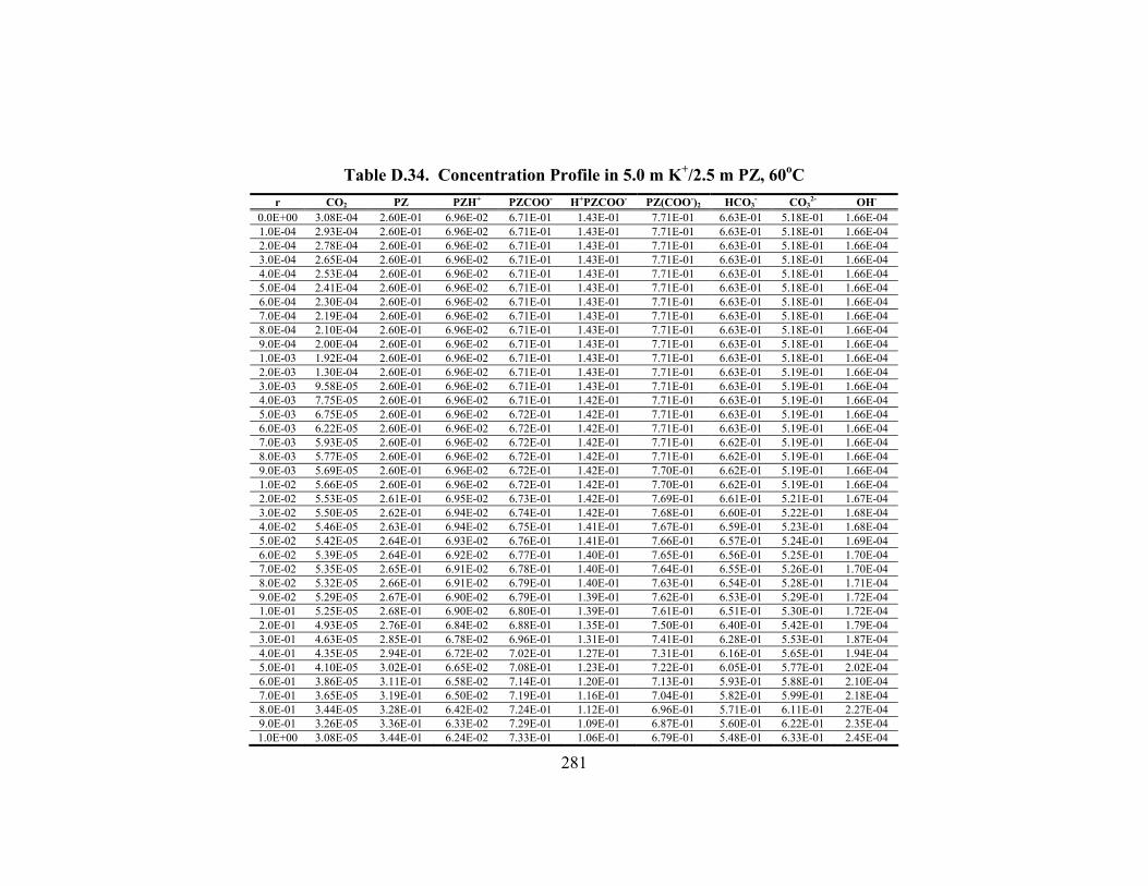
281
Table D.34. Concentration Profile in 5.0 m K+/2.5 m PZ, 60oC r CO2 PZ PZH+ PZCOO- H+PZCOO- PZ(COO-)2 HCO3
- CO32- OH-
0.0E+00 3.08E-04 2.60E-01 6.96E-02 6.71E-01 1.43E-01 7.71E-01 6.63E-01 5.18E-01 1.66E-04 1.0E-04 2.93E-04 2.60E-01 6.96E-02 6.71E-01 1.43E-01 7.71E-01 6.63E-01 5.18E-01 1.66E-04 2.0E-04 2.78E-04 2.60E-01 6.96E-02 6.71E-01 1.43E-01 7.71E-01 6.63E-01 5.18E-01 1.66E-04 3.0E-04 2.65E-04 2.60E-01 6.96E-02 6.71E-01 1.43E-01 7.71E-01 6.63E-01 5.18E-01 1.66E-04 4.0E-04 2.53E-04 2.60E-01 6.96E-02 6.71E-01 1.43E-01 7.71E-01 6.63E-01 5.18E-01 1.66E-04 5.0E-04 2.41E-04 2.60E-01 6.96E-02 6.71E-01 1.43E-01 7.71E-01 6.63E-01 5.18E-01 1.66E-04 6.0E-04 2.30E-04 2.60E-01 6.96E-02 6.71E-01 1.43E-01 7.71E-01 6.63E-01 5.18E-01 1.66E-04 7.0E-04 2.19E-04 2.60E-01 6.96E-02 6.71E-01 1.43E-01 7.71E-01 6.63E-01 5.18E-01 1.66E-04 8.0E-04 2.10E-04 2.60E-01 6.96E-02 6.71E-01 1.43E-01 7.71E-01 6.63E-01 5.18E-01 1.66E-04 9.0E-04 2.00E-04 2.60E-01 6.96E-02 6.71E-01 1.43E-01 7.71E-01 6.63E-01 5.18E-01 1.66E-04 1.0E-03 1.92E-04 2.60E-01 6.96E-02 6.71E-01 1.43E-01 7.71E-01 6.63E-01 5.18E-01 1.66E-04 2.0E-03 1.30E-04 2.60E-01 6.96E-02 6.71E-01 1.43E-01 7.71E-01 6.63E-01 5.19E-01 1.66E-04 3.0E-03 9.58E-05 2.60E-01 6.96E-02 6.71E-01 1.43E-01 7.71E-01 6.63E-01 5.19E-01 1.66E-04 4.0E-03 7.75E-05 2.60E-01 6.96E-02 6.71E-01 1.42E-01 7.71E-01 6.63E-01 5.19E-01 1.66E-04 5.0E-03 6.75E-05 2.60E-01 6.96E-02 6.72E-01 1.42E-01 7.71E-01 6.63E-01 5.19E-01 1.66E-04 6.0E-03 6.22E-05 2.60E-01 6.96E-02 6.72E-01 1.42E-01 7.71E-01 6.63E-01 5.19E-01 1.66E-04 7.0E-03 5.93E-05 2.60E-01 6.96E-02 6.72E-01 1.42E-01 7.71E-01 6.62E-01 5.19E-01 1.66E-04 8.0E-03 5.77E-05 2.60E-01 6.96E-02 6.72E-01 1.42E-01 7.71E-01 6.62E-01 5.19E-01 1.66E-04 9.0E-03 5.69E-05 2.60E-01 6.96E-02 6.72E-01 1.42E-01 7.70E-01 6.62E-01 5.19E-01 1.66E-04 1.0E-02 5.66E-05 2.60E-01 6.96E-02 6.72E-01 1.42E-01 7.70E-01 6.62E-01 5.19E-01 1.66E-04 2.0E-02 5.53E-05 2.61E-01 6.95E-02 6.73E-01 1.42E-01 7.69E-01 6.61E-01 5.21E-01 1.67E-04 3.0E-02 5.50E-05 2.62E-01 6.94E-02 6.74E-01 1.42E-01 7.68E-01 6.60E-01 5.22E-01 1.68E-04 4.0E-02 5.46E-05 2.63E-01 6.94E-02 6.75E-01 1.41E-01 7.67E-01 6.59E-01 5.23E-01 1.68E-04 5.0E-02 5.42E-05 2.64E-01 6.93E-02 6.76E-01 1.41E-01 7.66E-01 6.57E-01 5.24E-01 1.69E-04 6.0E-02 5.39E-05 2.64E-01 6.92E-02 6.77E-01 1.40E-01 7.65E-01 6.56E-01 5.25E-01 1.70E-04 7.0E-02 5.35E-05 2.65E-01 6.91E-02 6.78E-01 1.40E-01 7.64E-01 6.55E-01 5.26E-01 1.70E-04 8.0E-02 5.32E-05 2.66E-01 6.91E-02 6.79E-01 1.40E-01 7.63E-01 6.54E-01 5.28E-01 1.71E-04 9.0E-02 5.29E-05 2.67E-01 6.90E-02 6.79E-01 1.39E-01 7.62E-01 6.53E-01 5.29E-01 1.72E-04 1.0E-01 5.25E-05 2.68E-01 6.90E-02 6.80E-01 1.39E-01 7.61E-01 6.51E-01 5.30E-01 1.72E-04 2.0E-01 4.93E-05 2.76E-01 6.84E-02 6.88E-01 1.35E-01 7.50E-01 6.40E-01 5.42E-01 1.79E-04 3.0E-01 4.63E-05 2.85E-01 6.78E-02 6.96E-01 1.31E-01 7.41E-01 6.28E-01 5.53E-01 1.87E-04 4.0E-01 4.35E-05 2.94E-01 6.72E-02 7.02E-01 1.27E-01 7.31E-01 6.16E-01 5.65E-01 1.94E-04 5.0E-01 4.10E-05 3.02E-01 6.65E-02 7.08E-01 1.23E-01 7.22E-01 6.05E-01 5.77E-01 2.02E-04 6.0E-01 3.86E-05 3.11E-01 6.58E-02 7.14E-01 1.20E-01 7.13E-01 5.93E-01 5.88E-01 2.10E-04 7.0E-01 3.65E-05 3.19E-01 6.50E-02 7.19E-01 1.16E-01 7.04E-01 5.82E-01 5.99E-01 2.18E-04 8.0E-01 3.44E-05 3.28E-01 6.42E-02 7.24E-01 1.12E-01 6.96E-01 5.71E-01 6.11E-01 2.27E-04 9.0E-01 3.26E-05 3.36E-01 6.33E-02 7.29E-01 1.09E-01 6.87E-01 5.60E-01 6.22E-01 2.35E-04 1.0E+00 3.08E-05 3.44E-01 6.24E-02 7.33E-01 1.06E-01 6.79E-01 5.48E-01 6.33E-01 2.45E-04
282
Bibliography
Design Institute for Physical Properties (DIPPR). (2004). New York, American Institute of Chemical Engineers.
Energy Information Administration, (2002). Annual Energy Review 2002.
IEA Greenhouse Gas R&D Programme, (1995). Carbon Dioxide Utilisation.
IEA Greenhouse Gas R&D Programme, (2001). Putting Carbon Back into the Ground.
IEA Greenhouse Gas R&D Programme, (2002). Ocean Storage of CO2.
Kirk-Othmer Encyclopedia of Chemical Technology. (2004). Wiley.
Method of Separating CO2 and H2S from Gas Mixtures. (1959). U.S. Patent 2,886,405.
U.S. EPA, (2004). Inventory of U.S. Greenhouse Gas Emissions and Sinks: 1990-2002. Washington, D.C.
Ackermann, T. (1958). The Self-Dissociation of Water from Measurements of Molar Heats of Dissolved Electrolytes. Zeitschrift fuer Elektrochemie und Angewandte Physikalische Chemie 62: 411-419.
Albery, W. J., A. R. Greenwook and R. F. Kibble (1967). Diffusion Coefficients of Carboxylic Acids. Trans. Faraday Soc. 63(2): 360-368.
Al-Ghawas, H. A., D. P. Hagewiesche, G. Ruiz-Ibanez and O. C. Sandall (1989). Physicochemical Properties Important for Carbon Dioxide Absorption in Aqueous Methyldiethanolamine. J. Chem. Eng. Data 34(4): 385-391.
Al-Juaied, M. (2004). Carbon Dioxide Removal from Natural Gas by Membranes in the Presence of Heavy Hydrocarbons and by Aqueous Diglycolamine®/Morpholine. Ph.D. Dissertation. The University of Texas at Austin.
Alper, E. (1990a). Kinetics of Reactions of Carbon Dioxide with Diglycolamine and Morpholine. Chem. Eng. J. (Amsterdam, Netherlands) 44(2): 107-111.
Alper, E. (1990b). Reaction Mechanism and Kinetics of Aqueous Solutions of 2-Amino-2-Methyl-1-Propanol and Carbon Dioxide. Ind. Eng. Chem. Res. 29(8): 1725-1728.
Amdur, I., J. W. Irvine, E. A. Mason and J. Ross (1952). Diffusion Coefficients of the Systems CO2-CO2 and CO2-N2O. J. Chem. Phys. 20: 436-443.
283
Apelblat, A. (1992). The Vapor Pressures of Water over Saturated Aqueous Solutions of Barium Chloride, Magnesium Nitrate, Calcium Nitrate, Potassium Carbonate, and Zinc Sulfate, at Temperatures from 283 K to 313 K. J. Chem. Thermodyn. 24(6): 619-626.
Aroua, M. K. and R. M. Salleh (2004). Solubility of CO2 in Aqueous Piperazine and Its Modeling Using the Kent-Eisenberg Approach. Chem. Eng. Tech. 27(1): 65-70.
Aseyev, G. G. (1999). Electrolytes: Equilibria in Solutions and Phase Equilibria. Calculation of Multicomponent Systems and Experimental Data on the Activities of Water, Vapor Pressures, and Osmotic Coefficients. New York, Begell House.
Austgen, D. M. (1989). A Model of Vapor-Liquid Equilibria for Acid Gas-Alkanolamine-Water Systems. Ph.D. Dissertation. The University of Texas at Austin.
Barradas, R. G., M. C. Giordano and W. H. Sheffield (1971). Electrochemical Oxidation of Piperidine at Mercury and Platinum. Electrochim. Acta 16: 1235-1249.
Bates, S. J. and W. P. Baxter (1929). International Critical Tables of Numerical Data, Physics, Chemistry and Technology. New York, McGraw-Hill.
Bell, R. P. and A. F. Trotman-Dickenson (1949). Acid-Base Catalysis in Non-Aqueous Solvents. Part XII. The Amine-Catalysed Decomposition of Nitramide in Anisole Solution. J. Chem. Soc., Abs.: 1288-1297.
Benson, H. E., J. H. Field and R. M. Jimeson (1954). Carbon Dioxide Absorption Employing Hot Potassium Carbonate Solutions. Chem. Eng. Prog. 50: 356-364.
Benson, H. E., J. H. Field and W. P. Haynes (1956). Improved Process for Carbon Dioxide Absorption Uses Hot Carbonate Solutions. Chem. Eng. Prog. 52: 433-438.
Benson, S. W. (1960). The Foundations of Chemical Kinetics. New York, McGraw-Hill.
Bird, R. B., W. E. Stewart and E. N. Lightfoot (1960). Transport Phenomena. New York, Wiley.
Bishnoi, S. (2000). Carbon Dioxide Absorption and Solution Equilibrium in Piperazine Activated Methyldiethanolamine. Ph.D. Dissertation. The University of Texas at Austin.
284
Bishnoi, S. and G. T. Rochelle (2000). Absorption of Carbon Dioxide into Aqueous Piperazine: Reaction Kinetics, Mass Transfer and Solubility. Chem. Eng. Sci. 55(22): 5531-5543.
Bishnoi, S. and G. T. Rochelle (2002a). Absorption of Carbon Dioxide in Aqueous Piperazine/Methyldiethanolamine. AIChE J. 48(12): 2788-2799.
Bishnoi, S. and G. T. Rochelle (2002b). Thermodynamics of Piperazine/ Methyldiethanolamine/ Water/Carbon Dioxide. Ind. Eng. Chem. Res. 41(3): 604-612.
Blauwhoff, P. M. M., G.F. Versteeg and W. P. M. V. Swaaij (1984). A Study on the Reaction between CO2 and Alkanolamines in Aqueous Solutions. Chem. Eng. Sci. 39(2): 207-225.
Bocard, J. P. and B. J. Mayland (1962). New Charts for Hot Carbonate Process. Hydrocarbon Processing and Petroleum Refiner 41(4): 128-132.
Bosch, H., G. F. Versteeg and W. P. M. Van Swaaij (1989). Gas-Liquid Mass Transfer with Parallel Reversible Reactions-Ii. Absortpion of CO2 into Amine-Promoted Carbonate Solutions. Chem. Eng. Sci. 44(11): 2735-2743.
Bosch, H., G. F. Versteeg and W. P. M. Van Swaaij (1990). Kinetics of the Reaction of Carbon Dioxide with the Sterically Hindered Amine 2-Amino-2-Methylpropanol at 298 K. Chem. Eng. Sci. 45(5): 1167-1173.
Bronsted, J. N. and J. Teeter, C. E. (1924). On Kinetic Salt Effect. J. Phys. Chem. 28: 579-587.
Bronsted, J. N. and C. V. King (1925). Secondary Kinetic Salt Effect in the Case of Hydroxyl-Ion Catalysis. J. Am. Chem. Soc. 47: 2523-2531.
Bronsted, J. N. and E. A. Guggenheim (1927). Contribution to the Theory of Acid and Basic Catalysis. The Mutarotation of Glucose. J. Am. Chem. Soc. 49: 2554-2584.
Bronsted, J. N. (1928). Acid and Basic Catalysis. Chem. Rev. 5(3): 231-338.
Browning, G. J. and R. H. Weiland (1994). Physical Solubility of Carbon Dioxide in Aqueous Alkanolamines Via Nitrous Oxide Analogy. J. Chem. Eng. Data 39: 817-822.
Cabani, S., G. Conti, D. Giannessi and L. Lepori (1975). Thermodynamic Study of Aqueous Dilute Solutions of Organic Compounds. 3. Morpholines and Piperazines. J. Chem. Soc., Faraday Trans. 1 71(5): 1154-1160.
285
Cabani, S., G. Conti, P. Gianni and E. Matteoli (1976). Heat Capacity Changes in the Protonation of Amines in Aqueous Solution. Gazz. Chim. Ital. 106(3-6): 541-547.
Campbell, A. N. and S. Y. Lam (1973). The Densities, Viscosities, and Diffusion Coefficients of Solutions of Mono-, Di-, and Triethylamine in Water. Can. J. Chem. 51(24): 4005-4008.
Caplow, M. (1968). Kinetics of Carbamate Formation and Breakdown. J. Am. Chem. Soc. 90(24): 6795-6803.
Caracotsios, M. (1986). Model Parametric Sensitivity Analysis and Nonlinear Parameter Estimation. Theory and Applications. Ph.D. Dissertation. The University of Wisconsin.
Chen, C. C., H. I. Britt, J. F. Boston and L. B. Evans (1982). Local Composition Model for Excess Gibbs Energy of Electrolyte Systems. Part I: Single Solvent, Single Completely Dissociated Electrolyte Systems. AIChE J. 28(4): 588-596.
Chen, C. C. and L. B. Evans (1986). A Local Composition Model for the Excess Gibbs Energy of Aqueous Electrolyte Systems. AIChE J. 32(3): 444-454.
Chen, C.-C., H. I. Britt, J. F. Boston and L. B. Evans (1979). Extension and Application of the Pitzer Equation for Vapor-Liquid Equilibrium of Aqueous Electrolyte Systems with Molecular Solutes. AIChE J. 25(5): 820-831.
Chen, C.-C. and P. M. Mathias (2002). Applied Thermodynamics for Process Modeling. AIChE J. 48(2): 194-199.
Clarke, J. K. A. (1964). Kinetics of Absorption of Carbon Dioxide in Monoethanolamine Solutions at Short Contact Times. Ind. Eng. Chem. Fund. 3(3): 239-245.
Cook, H. L. and B. M. Lowe (1976). Viscosity B-Coefficients for Pinacol and Piperazine in Aqueous Solution at 25 and 35oC. Electrochim. Acta 21: 153-154.
Critchfield, J. E. (1988). CO2 Absorption/Desorption in Methyldiethanolamine Solutions Promoted with Monoethanolamine and Diethanolamine: Mass Transfer and Reaction Kinetics. Ph.D. Dissertation. The University of Texas at Austin.
Crooks, J. E. and J. P. Donnellan (1989). Kinetics and Mechanism of the Reaction between Carbon Dioxide and Amines in Aqueous Solution. J. Chem. Soc., Perkin Trans. 2(4): 331-333.
286
Crooks, J. E. and J. P. Donnellan (1990). Kinetics of the Reaction between Carbon Dioxide and Tertiary Amines. J. Org. Chem. 55(4): 1372-1374.
Cullinane, J. T. (2002). Carbon Dioxide Absorption in Aqueous Mixtures of Potassium Carbonate and Piperazine. M.S. Thesis. The University of Texas at Austin.
Cullinane, J. T. and G. T. Rochelle (2004). Thermodynamics of Aqueous Potassium Carbonate, Piperazine, and CO2 Mixtures. Fluid Phase Equilib. 227(2): 197-213.
Cuta, F. and F. Strafelda (1954). The Second Dissociation Constant of Carbonic Acid between 60 and 90o. Chemicke Listy pro Vedu a Prumysl 48: 1308-1313.
da Silva, E. F. and H. F. Svendsen (2004). Ab Initio Study of the Reaction of Carbamate Formation from CO2 and Alkanolamines. Ind. Eng. Chem. Res. 43(13): 3413-3418.
Danckwerts, P. V. (1951). Significance of Liquid-Film Coefficients in Gas Absorption. Ind. Eng. Chem. 43: 1460-1467.
Danckwerts, P. V. and M. M. Sharma (1966). Absorption of Carbon Dioxide into Solutions of Alkalies and Amines. Hydrogen Sulfide and Carbonyl Sulfide. Chemical Engineer (1904-20) No. 202: CE244-CE280.
Danckwerts, P. V. (1979). The Reaction of Carbon Dioxide with Ethanolamines. Chem. Eng. Sci. 34(4): 443-446.
Dang, H. (2001). CO2 Absorption Rate and Solubility in Monoethanolamine/ Piperazine/Water. M.S. Thesis. The University of Texas at Austin.
Donaldson, T. L. and Y. N. Nguyen (1980). Carbon Dioxide Reaction Kinetics and Transport in Aqueous Amine Membranes. Ind. Eng. Chem. Fund. 19(3): 260-266.
Edwards, T. J., G. Maurer, J. Newman and J. M. Prausnitz (1978). Vapor-Liquid Equilibria in Multicomponent Aqueous Solution of Volatile Weak Electrolytes. AIChE J. 24(6): 966-976.
Ellis, A. (1959). The Effect of Pressure on the First Dissociation Constant of "Carbonic Acid". J. Chem. Soc.: 3689-3699.
Enea, O. and G. Berthon (1973). Heats of Dissolution and Protonation of Piperazine and Its Derivatives in Different Water-Ethanol Mixtures. Electrochim. Acta 18(8): 579-582.
287
Ermatchkov, V., A. Perez-Salado Kamps and G. Maurer (2003). Chemical Equilibrium Constants for the Formation of Carbamates in (Carbon Dioxide + Piperazine + Water) from 1H-NMR-Spectroscopy. J. Chem. Thermodyn. 35(8): 1277-1289.
French, C. C. (1928). The Effect of Neutral Salts on Certain Catalytic Decompositions. J. Phys. Chem. 32: 401-414.
Glasscock, D. and G. T. Rochelle (1989). Numerical Simulation of Theories for Gas Absorption with Chemical Reaction. AIChE J. 35(8): 1271-1281.
Glasscock, D. (1990). Modeling and Experimental Study of Carbon Dioxide Absorption into Aqueous Alkanolamines. The University of Texas at Austin.
Gmehling, J., P. Rasmussen and A. Fredenslund (1982). Vapor-Liquid Equilibriums by UNIFAC Group Contribution. Revision and Extension. 2. Ind. Eng. Chem. Process Des. Dev. 21(1): 118-127.
Goncalves, F. A. and J. Kestin (1981). The Viscosity of Na2CO3 and K2CO3 Aqueous Solutions in the Range 20-60oC. Int. J. Thermophys. 2(4): 315-322.
Grube, G. and G. Schmid (1926). The Law of Neutral Salt Action in Concentrated Solutions. I. The Neutral Salt Action in the Acid Hydrolysis of Cyanamide. Z. Phys. Chem. 119: 19-45.
Harned, H. and R. Davis (1943). The Ionization Constant of Carbonic Acid in Water and the Solubility of Carbon Dioxide in Water and Aqueous Salt Solutions from 0 to 50oC. J. Am. Chem. Soc. 65: 2030-2037.
Harned, H. S. and R. A. Robinson (1940). Temperature Variation of the Ionization Constants of Weak Electrolytes. Trans. Faraday Soc. 36: 973-978.
Harned, H. S. and S. R. Scholes (1941). The Ionization Constant of HCO3- from 0 to
50oC. J. Am. Chem. Soc. 63: 1706-1709.
Harned, H. S. and B. B. Owen (1958). The Physical Chemistry of Electrolytic Solutions. New York, Reinhold Publishing.
Helgeson, H. C. and D. H. Kirkham (1974). Theoretical Prediction of the Thermodynamic Behavior of Aqueous Electrolytes at High Pressures and Temperatures. I. Thermodynamic/Electrostatic Properties of the Solvent. Am. J. Sci. 274(10): 1089-1198.
Hetzer, H. B., R. A. Robinson and R. G. Bates (1968). Dissociation Constants of Piperazinium Ion and Related Thermodynamic Quantities from 0 to 50o. J. Phys. Chem. 72(6): 2081-2086.
288
Higbie, R. (1935). The Rate of Absorption of a Pure Gas into a Still Liquid During Short Periods of Exposure. Trans. Am. Inst. Chem. Engrs. 31: 365-389.
Hikita, H. and S. Asai (1963). Gas Absorption with (M,N)Th Order Irreversible Chemical Reactions. Kagaku Kogaku 27(11): 823-830.
Hikita, H., S. Asai, H. Ishikawa and M. Honda (1977). The Kinetics of Reactions of Carbon Dioxide with Monoethanolamine, Diethanolamine and Triethanolamine by a Rapid Mixing Method. Chem. Eng. J. 13: 7-12.
Hikita, H., H. Ishikawa, T. Murakami and T. Ishii (1981). Densities, Viscosities and Amine Diffusivities of Aqueous MIPA, DIPA, DGA and EDA Solutions. J. Chem. Eng. Jap. 14(5): 411-413.
Hitchcock, L. B. and J. S. Mcilhenny (1935). Viscosity and Density of Pure Alkaline Solutions and Their Mixtures. Ind. Eng. Chem. 27(4): 461-466.
Hobler, T. (1966). Mass Transfer and Absorbers. Oxford, Pergamon Press.
Jensen, A., M. B. Jensen and C. Faurholt (1952). Carbamates. VIII. The Carbamates of Benzylamine, Piperidine, and Alanine. Acta Chem. Scand. 6: 1073-1085.
Jensen, A. and R. Christensen (1955). Carbamates. XI. The Carbamate of Ethylenediamine. Acta Chem. Scand. 9: 486-492.
Jensen, M. B., E. Jorgensen and C. Fourholt (1954). Reactions between Carbon Dioxide and Amino Alcohols. I. Monoethanolamine and Diethanolamine. Acta Chem. Scand. 8(7): 1137-1140.
Joosten, G. E. H. and P. V. Danckwerts (1972). Solubility and Diffusivity of Nitrous Oxide in Equimolar Potassium Carbonate-Potassium Bicarbonate Solutions at 25o and 1 Atm. J. Chem. Eng. Data 17(4): 452-454.
Jorgensen, E. (1956). Reactions between Carbon Dioxide and Amino Alcohols. III. Diethanolamine. Acta Chem. Scand. 10: 747-55.
Kamps, A. P.-S., J. Xia and G. Maurer (2003). Solubility of CO2 in (H2O + Piperazine) and in (H2O + MDEA + Piperazine). AIChE J. 49(10): 2662-2670.
King, C. J. (1966). Turbulent Liquid-Phase Mass Transfer at a Free Gas-Liquid Interface. Ind. Eng. Chem. Fund. 5(1): 1-8.
Kloosterman, E. G., S. M. De Vries, H. Kalsbeek and B. Drinkenburg (1987). Influence of Ionic Strength on the Absorption of Carbon Dioxide in

289
Carbonate/Bicarbonate Buffer Solutions. Ind. Eng. Chem. Res. 26(11): 2216-2222.
Kohl, A. L. and F. C. Riesenfeld (1985). Gas Purification. Houston, Gulf Publishing.
Kumar, P. S., J. A. Hogendoorn, G. F. Versteeg and P. H. M. Feron (2003). Kinetics of the Reaction of CO2 with Aqueous Potassium Salt of Taurine and Glycine. AIChE J. 49(1): 203-213.
Laddha, S. S. and P. V. Danckwerts (1981). Reaction of Carbon Dioxide with Ethanolamines. Kinetics from Gas-Absorption. Chem. Eng. Sci. 36(3): 479-482.
Laddha, S. S. and P. V. Danckwerts (1982). The Absorption of Carbon Dioxide by Amine-Potash Solutions. Chem. Eng. Sci. 37(5): 665-667.
Le Bas, G. (1915). The Molecular Volumes of Liquid Chemical Compounds. London, Longman Green.
Lee, M.-J., Y.-K. Chang, H.-M. Lin and C.-H. Chen (1997). Solid-Liquid Equilibria for 4-Methoxyphenol with Catechol, Ethylenediamine, or Piperazine. J. Chem. Eng. Data 42(2): 349-352.
Lewis, W. K. and W. G. Whitman (1924). Principles of Gas Absorption. Ind. Eng. Chem. 16: 1215-1220.
Lide, D. R., Ed. (2000). CRC Handbook of Chemistry and Physics. London, CRC Press.
Linke, W. F. and A. Seidell (1966). Solubilities of Inorganic and Metal Organic Compounds Vol. II. 4th Ed.
Littel, R. J., M. Bos and G. J. Knoop (1990a). Dissociation Constants of Some Alkanolamines at 293, 303, 318, and 333 K. J. Chem. Eng. Data 35(3): 276-277.
Littel, R. J., W. P. M. Van Swaaij and G. F. Versteeg (1990b). Kinetics of Carbon Dioxide with Tertiary Amines in Aqueous Solution. AIChE J. 36(11): 1633-1640.
Littel, R. J. (1991). Selective Carbonyl Sulfide Removal in Acid Gas Treating Processes. Ph.D. Dissertation. Twente University.
Littel, R. J., G. F. Versteeg and W. P. M. Van Swaaij (1992a). Kinetics of Carbon Dioxide with Primary and Secondary Amines in Aqueous Solutions. I. Zwitterion Deprotonation Kinetics for Dea and Dipa in Aqueous Blends of Alkanolamines. Chem. Eng. Sci. 47(8): 2027-2035.
290
Littel, R. J., G. F. Versteeg and W. P. M. Van Swaaij (1992b). Solubility and Diffusivity Data for the Absorption of COS, CO2, and N2O in Amine Solutions. J. Chem. Eng. Data 37: 49-55.
Littel, R. J., G. F. Versteeg and W. P. M. Van Swaaij (1992c). Kinetics of CO2 with Primary and Secondary Amines in Aqueous Solutions--II. Influence of Temperature on Zwitterion Formation and Deprotonation Rates. Chem. Eng. Sci. 47(8): 2037-2045.
Liu, J., K. Sepehrnoori and G. A. Pope (1995). A High-Resolution Finite-Difference Scheme for Nonuniform Grids. Appl. Math. Modeling 19: 163-172.
Livingston, R. (1930). An Introduction to Chemical Catalysis in Homogeneous Systems. J. Chem. Educ. 7(12): 2887-2903.
Mahajani, V. V. and P. V. Danckwerts (1982). Carbamate-Bicarbonate Equilibrium for Several Amines at 100oC in 30% Potash. Chem. Eng. Sci. 37(6): 943-944.
Mahajani, V. V. and P. V. Danckwerts (1983). The Stripping of Carbon Dioxide from Amine-Promoted Potash Solutions at 100oC. Chem. Eng. Sci. 38(2): 321-327.
Mahajani, V. V. and J. B. Joshi (1988). Kinetics of Reaction between Carbon Dioxide and Alkanolamines. Gas Sep. Purif. 2.
Mock, B., L. B. Evans and C. C. Chen (1986). Thermodynamic Representation of Phase Equilibria of Mixed-Solvent Electrolyte Systems. AIChE J. 32(10): 1655-1664.
Moniuk, W. and R. Pohorecki (1991). Viscosity and Density of Sodium and Potassium Alkaline Solutions. Hungarian J. Ind. Chem. Veszprem 19: 175-178.
Mshewa, M. M. (1995). Carbon Dioxide Desorption/Absorption with Aqueous Mixtures of Methyldiethanolamine and Diethanolamine at 40 to 120oC. Ph.D. Dissertation. The University of Texas at Austin.
Nijsing, R. A. T. O., R. H. Hendriksz and H. Kramers (1959). Absorption of Carbon Dioxide in Jets and Falling Films of Electrolyte Solutions, with and without Chemical Reaction. Chem. Eng. Sci. 10: 88-104.
Olson, A. R. and T. R. Simonson (1949). Rates of Ionic Reactions in Aqueous Solutions. J. Chem. Phys. 17(12): 1167-1173.
Oscarson, J. L., G. Wu, P. W. Faux, R. M. Izatt and J. J. Christensen (1989a). Thermodynamics of Protonation of Alkanolamines in Aqueous Solution to 325 Degc. Thermochim. Acta 154(1): 119-127.
291
Oscarson, J. L., R. H. Van Dam, J. J. Christensen and R. M. Izatt (1989b). Enthalpies of Absorption of Carbon Dioxide in Aqueous Diethanolamine Solutions. Thermochim. Acta 146: 107-114.
Pacheco, M. A. (1998). Mass Transfer, Kinetics and Rate-Based Modeling of Reactive Absorption. Ph.D. Dissertation. The University of Texas at Austin.
Pagano, J. M., D. E. Goldberg and W. C. Fernelius (1961). A Thermodynamic Study of Homopiperazine, Piperazine, and N-(2-Aminoethyl)Piperazine and Their Complexes with Copper(II) Ion. J. Phys. Chem. 65: 1062-1064.
Paoletti, P., M. Ciampolini and A. Vacca (1963). Thermochemical Studies. VII. Heats and Entropies of Stepwise Neutralization of Piperazine and Triethylenetetramine. J. Phys. Chem. 67: 1065-1067.
Penny, D. E. and T. J. Ritter (1983). Kinetic Study of the Reaction between Carbon Dioxide and Primary Amines. J. Chem. Soc., Faraday Trans. 1 79(9): 2103-2109.
Perrin, D. D., B. Dempsey and E. P. Serjeant (1981). pKa Prediction for Organic Acids and Bases: 6-9, 36-37.
Pigford, R. L. (1941). Counter-Diffusion in a Wetted-Wall Column. Ph.D. Dissertation. University of Illinois.
Pinsent, B. R. W., L. Pearson and F. J. W. Roughton (1956). Kinetics of Combination of Carbon Dioxide with Hydroxide Ions. Trans. Faraday Soc. 52: 1512-1520.
Pohorecki, R. and W. Moniuk (1988). Kinetics of Reaction between Carbon Dioxide and Hydroxyl Ions in Aqueous Electrolyte Solutions. Chem. Eng. Sci. 43(7): 1677-1684.
Pohorecki, R., D. T. Xoan and W. Moniuk (1988). Study of Carbon Dioxide Absorption in Aqueous Solution of Potassium Carbonate Containing Ethylaminoethanol. II. Kinetic Relations for 2-(Ethylamino)Ethanol. Chemiczna i Procesowa 9(4): 667-680.
Posey, M. L. (1996). Thermodynamic Model for Acid Gas Loaded Aqueous Alkanolamine Solutions. Ph.D. Dissertation. The University of Texas at Austin.
Prasher, B. D. and A. L. Fricke (1974). Mass Transfer at a Free Gas-Liquid Interface in Turbulent Thin Films. Ind. Eng. Chem. Process Des. Dev. 13(4): 336-340.
Puchkov, L. V. and V. V. Kurochkina (1970). Saturated Vapor Pressure over Aqueous Solutions of Potassium Carbonate. Zhur. Priklad. Khim. 43(1): 181-183.
292
Rao, A. B. and E. S. Rubin (2002). A Technical, Economic, and Environmental Assessment of Amine-Based CO2 Capture Technology for Power Plant Greenhouse Gas Control. Environ. Sci. Technol. 36(20): 4467-4475.
Redlich, O. and J. N. S. Kwong (1948). On the Thermodynamics of Solutions. V. An Equation of State. Fugacities of Gaseous Solutions. Chem. Rev. 44: 233-244.
Renon, H. and J. M. Prausnitz (1968). Local Compositions in Thermodynamic Excess Functions for Liquid Mixtures. AIChE J. 14(1): 135-144.
Rinker, E. B., S. S. Ashour and O. C. Sandall (1995). Kinetics and Modeling of Carbon Dioxide Absorption into Aqueous Solutions of N-Methyldiethanolamine. Chem. Eng. Sci. 50(5): 755-768.
Rochelle, G. T., S. Bishnoi, S. Chi, H. Dang and J. Santos, U.S. Department of Energy, (2001). Research Needs for CO2 Capture from Flue Gas by Aqueous Absorption/Stripping. Pittsburg. DE-AF26-99FT01029.
Roy, R. N., J. J. Gibbons, R. Williams, L. Godwin, G. Baker, J. M. Simonson and K. S. Pitzer (1984). The Thermodynamics of Aqueous Carbonate Solutions. II. Mixtures of Potassium Carbonate, Bicarbonate, and Chloride. J. Chem. Thermodyn. 16(4): 303-315.
Rubin, E. S., A. B. Rao and C. Chen (2004). Comparative Assessments of Fossil Fuel Power Plants with CO2 Capture and Storage. 7th International conference on Greenhouse Gas Control Technologies, Vancouver, Canada.
Ryzhenko, B. N. (1963). Dissociation Constants for Carbonic Acid at Elevated Temperatures. Doklady Akademii Nauk SSSR 149: 639-641.
Sada, E., H. Kumazawa and M. A. Butt (1976a). Gas Absorption with Consecutive Chemical Reaction: Absorption of Carbon Dioxide into Aqueous Amine Solutions. Can. J. Chem. Eng. 54(5): 421-424.
Sada, E., H. Kumazawa and M. A. Butt (1976b). Chemical Absorption Kinetics over a Wide Range of Contact Time: Absorption of Carbon Dioxide into Aqueous Solutions of Monoethanolamine. AIChE J. 22(1): 196-198.
Sada, E., H. Kumazawa and M. A. Butt (1978). Solubility and Diffusivity of Gases in Aqueous Solutions of Amines. J. Chem. Eng. Data 23(2): 161-163.
Sarbar, M., A. K. Covington, R. L. Nuttall and R. N. Goldberg (1982). Activity and Osmotic Coefficients of Aqueous Potassium Carbonate. J. Chem. Thermodyn. 14(7): 695-702.
293
Sartori, G. and D. W. Savage (1983). Sterically Hindered Amines for Carbon Dioxide Removal from Gases. Ind. Eng. Chem. Fund. 22(2): 239-249.
Savage, D. W., G. Sartori and G. Astarita (1984). Amines as Rate Promoters for Carbon Dioxide Hydrolysis. Faraday Discuss. Chem. Soc.(77): 17-31.
Schramke, J. A., S. F. Murphy, W. J. Doucette and W. D. Hintze (1999). Prediction of Aqueous Diffusion Coefficients for Organic Compounds at 25oC. Chemosphere 38(10): 2381-2406.
Schwarzenbach, D. (1968). Structure of Piperazine Hexahydrate. J. Chem. Phys. 48(9): 4134-4140.
Schwarzenbach, V. G., B. Maissen and H. Ackermann (1952). Metallkomplexe Mit Polyaminen VII: Diamine Und Silber(I). Helv. Chim. Acta 35(289): 2333-2336.
Seo, D. J. and W. H. Hong (2000). Effect of Piperazine on the Kinetics of Carbon Dioxide with Aqueous Solutions of 2-Amino-2-Methyl-1-Propanol. Ind. Eng. Chem. Res. 39(6): 2062-2067.
Sharma, M. M. (1965). Kinetics of Reactions of Carbonyl Sulphide and Carbon Dioxide with Amines and Catalysis by Bronsted Bases of the Hydrolysis of COS. Trans. Faraday Soc. 61: 681-687.
Shrier, A. L. and P. V. Danckwerts (1969). Carbon Dioxide Absorption into Amine Promoted Potash Solutions. Ind. Eng. Chem. Fund. 8(3): 415-423.
Simonson, J. M., R. N. Roy and J. J. Gibbons (1987). Thermodynamics of Aqueous Mixed Potassium Carbonate, Bicarbonate, and Chloride Solutions to 368 K. J. Chem. Eng. Data 32(1): 41-45.
Smith, J. M., H. C. Van Ness and M. M. Abbott (1996). Introduction to Chemical Engineering Thermodynamics. New York, McGraw-Hill.
Smith, W. R. and R. W. Missen (1988). Strategies for Solving the Chemical Equilibrium Problem and an Efficient Microcomputer-Based Algorithm. Can. J. Chem. Eng. 66(4): 591-598.
Snijder, E. D., M. J. M. Te Riele, G. F. Versteeg and W. P. M. Van Swaaij (1993). Diffusion Coefficients of Several Aqueous Alkanolamine Solutions. J. Chem. Eng. Data 38(3): 475-480.
Soave, G. (1972). Equilibrium Constants from a Modified Redlich-Kwong Equation of State. Chem. Eng. Sci. 27(6): 1197-1203.
294
Steele, W. V., R. D. Chirico, S. E. Knipmeyer, A. Nguyen and N. K. Smith (1997). Thermodynamic Properties and Ideal-Gas Enthalpies of Formation for Dicyclohexyl Sulfide, Diethylenetriamine, Di-N-Octyl Sulfide, Dimethyl Carbonate, Piperazine, Hexachloroprop-1-Ene, Tetrakis(Dimethylamino) Ethylene, N,N'-Bis-(2-Hydroxyethyl)Ethylenediamine, and 1,2,4-Triazolo[1,5-a]Pyrimidine. J. Chem. Eng. Data 42(6): 1037-1052.
Tamimi, A., E. B. Rinker and O. C. Sandall (1994a). Diffusivity of Nitrous Oxide in Aqueous Solutions of N-Methyldiethanolamine and Diethanolamine from 293 to 368 K. J. Chem. Eng. Data 39(2): 396-398.
Tamimi, A., E. B. Rinker and O. C. Sandall (1994b). Diffusion Coefficients for Hydrogen Sulfide, Carbon Dioxide, and Nitrous Oxide in Water over the Temperature Range 293-368 K. J. Chem. Eng. Data 39(2): 330-332.
Toman, J. J. and G. T. Rochelle (1989). Carbon Dioxide Absorption Rates and Physical Solubility in 50% Aqueous Methyldiethanolamine Partially Neutralized with Sulfuric Acid. Unpublished.
Tosh, J. S., J. H. Field, H. E. Benson and W. P. Haynes (1959). Equilibrium Study of the System Potassium Carbonate, Potassium Bicarbonate, Carbon Dioxide, and Water. U.S. Bur. Mines, Rept. Invest. No. 5484: 23 pp.
Trotman-Dickenson, A. F. (1949). The Basic Strength of Amines. J. Chem. Soc., Abs.: 1293-1297.
Tseng, P. C., W. S. Ho and D. W. Savage (1988). Carbon Dioxide Absorption into Promoted Carbonate Solutions. AIChE J. 34(6): 922-931.
Van Der Wielen, L. A. M., J. H. Zomerdijk and K. C. A. M. Luyben (1997). Diffusivities of Organic Electrolytes in Water. Chem. Eng. J. 66: 111-121.
Vazquez, P. G., F. Chenlo, R. Moreira and P. Pardo (1994). Viscosity of the Following Na2CO3, NaHCO3, K2CO3, KHCO3, Na2CO3-NaHCO3, and K2CO3-KHCO3 Solutions Important in Absorption Processes. Afinidad Li May-June: 211-216.
Verevkin, S. P. (1998). Thermochemistry of Amines: Strain in Six-Membered Rings from Experimental Standard Molar Enthalpies of Formation of Morpholines and Piperazines. J. Chem. Thermodyn. 30(9): 1069-1079.
Versteeg, G. F. (1987). Mass Transfer and Chemical Reaction Kinetics in Acid Gas Treating Processes. Ph.D. Dissertation. Twente University.
295
Versteeg, G. F. and W. P. M. Van Swaaij (1988a). On the Kinetics between Carbon Dioxide and Alkanolamines Both in Aqueous and Non-Aqueous Solutions - II. Tertiary Amines. Chem. Eng. Sci. 43(3): 587-591.
Versteeg, G. F. and W. P. M. Van Swaaij (1988b). Solubility and Diffusivity of Acid Gases (CO2, N2O) in Aqueous Alkanolamine Solutions. J. Chem. Eng. Data 33(1): 29-34.
Versteeg, G. F. and M. H. Oyevaar (1989). The Reaction between Carbon Dioxide and Diethanolamine at 298 K. Chem. Eng. Sci. 44(5): 1264-1268.
Versteeg, G. F., L. A. J. Van Duck and W. P. M. Van Swaaij (1996). On the Kinetics between CO2 and Alkanolamines Both in Aqueous and Nonaqueous Solutions. An Overview. Chem. Eng. Commun. 144: 113-158.
Vivian, J. E. and D. W. Peaceman (1956). Liquid-Side Resistance in Gas Absorption. AIChE J. 2: 437-443.
Weiland, R. H., J. C. Dingman, D. B. Cronin and G. J. Browning (1998). Density and Viscosity of Some Partially Carbonated Aqueous Alkanolamine Solutions and Their Blends. J. Chem. Eng. Data 43(3): 378-382.
Weisenberger, S. and A. Schumpe (1996). Estimation of Gas Solubilities in Salt Solutions at Temperatures from 273 K to 363 K. AIChE J. 42(1): 298-300.
Wilke, C. R. and P. Chang (1955). Correlation of Diffusion Coefficients in Dilute Solutions. AIChE J. 1: 264-270.
Wilson, G. M. (1964). Vapor-Liquid Equilibrium. XI. A New Expression for the Excess Free Energy of Mixing. J. Am. Chem. Soc. 86(2): 127-130.
Wilson, H. L. and W. V. Wilding (1994). Vapor-Liquid and Liquid-Liquid Equilibrium Measurements on Twenty-Two Binary Mixtures. Experimental Results for DIPPR 1990-91 Projects on Phase Equilibria and Pure Component Properties. J. R. Cunningham and D. K. Jones: 63-115.
Xu, S., Y.-W. Wang, F. D. Otto and A. E. Mather (1993). Kinetics of the Reaction of Carbon Dioxide with Aqueous 2-Piperidineethanol Solutions. AIChE J. 39(10): 1721-1725.
Yaws, C. L. (1994). Handbook of Vapor Pressure. Houston, Gulf Publishing.
Yih, S. M. and K. P. Shen (1988). Kinetics of Carbon Dioxide Reaction with Sterically Hindered 2-Amino-2-Methyl-1-Propanol Aqueous Solutions. Ind. Eng. Chem. Res. 27(12): 2237-2241.
296
Vita
John Timothy Cullinane was born on September 17, 1976 in Jackson,
Mississippi to Murdock John Cullinane, Jr. and Gwendolyn Anthony Cullinane. After
graduating from Clinton High School in Clinton, Mississippi in 1995, he enrolled at
Mississippi State University. As an undergraduate, he participated in the cooperative
education program for three semesters as an employee of The Dow Chemical Company
in Plaquemine, Louisiana and Freeport, Texas. He graduated summa cum laude with a
Bachelor of Science in chemical engineering in December of 1999. His graduate
studies at The University of Texas at Austin commenced in August 2000. In the
interim, he served as teaching assistant at Mississippi State University and an
engineering intern at the Engineering Research and Development Center in Vicksburg,
Mississippi. In May of 2002, he received a Master of Science from The University of
Texas at Austin. He has accepted a full-time employment offer with ExxonMobil
Upstream Research Company in Houston, Texas.
Permanent Address: 104 Concord Drive
Clinton, Mississippi 39056
This dissertation was typed by the author.