DRAFT

White PaperAdvance Notice of Wholesale

Electricity Prices:Recommended Solutions

and

Austin, TexasOctober 30, 2010

DRAFT

Prepared under the direction of:

Jay Zarnikau, Ph.D.Frontier Associates

Parviz Adib, Ph.D.Economead Energy Consulting

DRAFTTable of Contents

1 Introduction................................................................................................................2

2 Consumers and Retailers Need Advance Notice of Prices to Assure the Market Operates Efficiently...........................................................................................................3

3 The Importance of Demand Response.....................................................................4

4 The Market Benefits from the Current System of Providing Advance Notice of Wholesale Prices................................................................................................................8

5 Advance Notice of Prices in the Future Nodal Market........................................10

6 Price Responsive Loads and Price Notice Periods in Other Wholesale Electricity Markets..........................................................................................................13

7 Recommended Solutions.........................................................................................15

7.1 Providing Advance Notice of Settlement Prices....................................................15

7.2 Using the SCED interval as the Settlement Interval for Loads That Have or Are Willing to Acquire IDRs.................................................................................................21

7.3 Providing Informational Price Forecasts During the Operating Day..................22

7.4 Establishing a Special Economic Demand Response Program Based on Binding Forecasts of Prices........................................................................................................23

7.5 Allowing Price Responsive Loads to be Modeled Directly in SCED Model.........24

Appendix I: Price Responsive Loads in Selected Wholesale Electricity Markets.......1

Appendix II: RTO/ISO Price Responsive Load Programs (Baseline and Performance)......................................................................................................................1

Appendix III: Regression Statistics for Relationship between Wholesale Prices and Deployments of Regulation...............................................................................................1

Appendix IV: Regression Statistics for Relationship between Obligations for Regulation and Deployments of Regulation....................................................................1

Appendix V: Zonal MCPE and MWs Obtained, 2008 and 2009 Balancing Energy Services Market.................................................................................................................1

Appendix VI: Possible Increase in the Cost of Regulation Down due to Demand-Side Response to Prices...............................................................................................................1

Frontier Associates & 1Economead Energy Consulting

DRAFT

Advance Notice of Wholesale Electricity PricesSome Practical Solutions

1 Introduction

Demand response to price changes is critical for the success of any competitive market. It plays a unique role in balancing demand and supply for any product and service during scarcity conditions while mitigating any potential abuse of market power by dominant suppliers. Timely advance notice of price (ex-ante pricing) plays a crucial role in enabling consumers to make informed decisions regarding their consumption behavior. In an affidavit filed with the Federal Energy Regulatory Commission (FERC) regarding price-responsive demand side activities in wholesale electricity markets, the father of economic deregulation in the United States, Dr. Alfred E. Kahn, emphasizes that “any increase in the efficient responsiveness of demand (to prices competitively determined, as in the ISO-conducted auctions) will move us in the direction of correcting the most severe deficiency in most such markets in the US, the lack of an adequately, price-responsive demand side.”1

In electricity markets, price signals are typically provided through a Day Ahead Market (DAM) where electricity is traded and prices are announced publicly. While DAM prices are helpful, there is no guarantee that similar prices will materialize during operation of the Real Time Market (RTM). In fact, different prices from those announced in DAM should be expected, particularly for wholesale electricity markets that are designed as energy-only markets with no formal capacity payments. Therefore, it is crucial that prices are also provided before real time operating intervals to ensure effective participation in the market by price responsive loads.

The Electric Reliability Council of Texas (ERCOT), currently considered among the best for voluntary price response due to its ex-ante pricing, will begin operating an energy-only nodal market on December 1, 2010. Meanwhile the market’s transmission and distribution utilities are deploying advanced meters for the primary purpose of extending demand response opportunities to the majority of consumers within ERCOT. This white paper addresses a key flaw in the design of the market – the absence of ex-ante pricing during RTM operation. This flaw will seriously hinder voluntary price response by loads. Solutions and recommendations are provided.

1 PennEnergy, Renowned Regulatory Economist Supports FERC Proposal for Demand Response, August 31, 2010. Also available at: http://www.pennenergy.com/index/power/display/1249454709/articles/pennenergy/power/grid/2010/08/renowned-regulatory.html .

Frontier Associates & 2Economead Energy Consulting

DRAFT

2 Consumers and Retailers Need Advance Notice of Prices to Assure the Market Operates Efficiently

In its original decision adopting the Zonal Protocols developed through ERCOT’s stakeholder process, the Public Utility Commission of Texas (PUCT) endorsed the notion that prices should be provided to consumers in advance of an operating interval. This was intended to enhance voluntary price responses by customers.2 Larger price responsive consumers have been responding to electricity prices since the start of retail competition in January 2002. Such responses have been possible in the current zonal market due to the requirement that ERCOT announce prices ten minutes3 in advance of each 15-minute operating interval. This market feature will disappear under ERCOT’s new nodal market design, because ERCOT will no longer be providing ex-ante prices. Instead, only ex-post prices will be provided. There will be a lag of 30 to 60 seconds following the start of a Security-Constrained Economic Dispatch (SCED) interval before the average zonal price for that 5-minute SCED interval will be known by consumers. Furthermore, as discussed in Section 5, because loads will continue to be settled on a 15-minute interval based on each load’s weighted average usage over a 15-minute period, any attempted response to the ex-post 5-minute zonal SCED price received by the consumer will not be reflected accurately in the price the consumer is charged for the whole 15-minute settlement interval.

Many large industrial energy consumers taking service under Market Clearing Price of Energy Products, “MCPE Products,” in the current zonal market respond to ex-ante wholesale prices. Through their actions, system demand is reduced during periods of high prices. This results in lower energy costs not only for those price-responsive consumers, but for all other consumers as well because there will be less need for inefficient resources to operate.

In the new nodal market, periods of high prices and overall price volatility are to be expected, since the market is designed as an energy-only market and has no formal capacity payment requirement. Furthermore, the ERCOT nodal market will have the highest offer (price) cap of all competitive wholesale electricity markets in this country.4

The magnitude of the resulting price volatility risk for consumers underscores how essential ex-ante pricing is to the ability of price responsive loads to avoid anomalous price spikes. Ex-ante pricing becomes even more important during RTM operation when actual consumption of electricity takes place and the system operator is engaged in balancing demand and supply while maintaining system reliability.

ERCOT’s wholesale electricity market, particularly its retail operation, has seen significant improvement over the last nine years. The loss of RTM ex-ante pricing is a 2 PUCT, Final Order in Docket No. 23220: Petition of the Electric Reliability Council of Texas for

Approval of the ERCOT Protocols.3 While a 10-minute notice is expected, prices are reflected on the website about 8 or 9 minutes in

advance.4 ERCOT currently has a $2,250 per MWh or MW offer cap which is expected to increase to $3,000 per

MWh or MW a couple of months after nodal operations begin on December 1, 2010.

Frontier Associates & 3Economead Energy Consulting

DRAFTmajor step backward in ERCOT’s market design that will result in a less robust competitive market. Absent accurate price information and advance notice, energy consumers will be unable to curtail demand in response to real-time market fluctuations and unexpected high prices. This will limit the ability of consumers to control their electricity costs and will place upward pressure on overall prices in the competitive market.

3 The Importance of Demand Response

The importance of demand response in power markets is widely recognized.5 When energy consumers have an opportunity to respond to wholesale prices, a variety of policy objectives are advanced. System operating and investment costs are reduced when energy consumers are encouraged to shift their consumption of electricity from high price periods to hours when electricity can be supplied to consumers at a lower cost. Uneconomical price spikes can be reduced or avoided. Market power can be held in check.6 Economic efficiency requires that consumers know the price they will be paying before making purchase decisions. Some forms of demand response can provide environmental benefits by reducing power plant emissions during “ozone action days” or other periods of impaired air quality.  Some residential load management programs may have energy efficiency features, by reducing the overall energy used for water heating, pool pumping, or air conditioning.   Furthermore, other environmental and operational benefits are expected from demand response in a wholesale electricity market.7 The North American Electric Reliability Corporation (NERC) has concluded “Successful climate change initiatives must support the development and reliable integration of demand-side resources.”8

Demand response is especially important in light of the decision of the PUCT to pursue an energy-only resource adequacy mechanism. As noted in the Commission Staff’s Strawman Resource Adequacy Rule: “Increasing the responsiveness of demand is a goal of this rule and critical to the success of an energy-only resource adequacy mechanism.”9

This was reemphasized in its final Resource Adequacy mechanism, Subst. R. §25.505.10 5 Potomac Economics, Comments on Demand Response Compensation in Organized Wholesale Energy

Markets, FERC NOPR in Rulemaking Project RM10-17, May 13, 2010, pp. 2-3. Also available at: http://elibrary.ferc.gov/idmws/file_list.asp .

6 Michael Rosenzweig, Hamish Fraser, Jonathan Falk, and Sarah Voll, “Market Power and Demand Responsiveness: Letting Customers Protect Themselves,” The Electricity Journal, May 2003.

7 For a summary of the benefits of demand responses, see a presentation by Richard Sedano titled Using Demand Response to Reduce Power Supply Costs, The Regulatory Assistance Project, June 22, 2010. Also available at: http://www.raponline.org/showpdf.asp?PDF_URL="docs/RAP_Sedano_APPA_UsingDemandResponsetoReducePowerSupplyCosts_2010_06_22.pdf" .

8 NERC, Special Report: Electric Industry Concerns on the Reliability Impacts of Climate Change Initiatives, New Jersey, November 2008, p. 16. Also available at: http://www.nerc.com/files/2008-Climate-Initiatives-Report.pdf .

9 PUCT, Project No. 24255: Rulemaking Concerning Planning Reserve Margin Requirements, Staff’s Resource Adequacy Strawman, Wholesale Market Oversight Division, August 19, 2005, p. 2.

10 PUCT Substantive Rule 25.505, Resource Adequacy in the Electric Reliability Council of Texas Power Region, finalized on August 16, 2007. The latest version is available at: http://www.puc.state.tx.us/rules/subrules/electric/25.505/25.505.pdf .

Frontier Associates & 4Economead Energy Consulting

DRAFTAs noted by Federal Energy Regulatory Commission (FERC), “[d]emand response is essential in competitive markets, to assure the efficient interaction of supply and demand, as a check on supplier and locational market power, and as an opportunity for choice by wholesale and end-use customers.”11

The United States Congress affirmed the importance of expanding demand response opportunities:

It is the policy of the United States that time-based pricing and other forms of demand response, whereby electricity customers are provided with electricity price signals and the ability to benefit by responding to them, shall be encouraged, the deployment of such technology and devices that enable electricity customers to participate in such pricing and demand response systems shall be facilitated, and unnecessary barriers to demand response participation in energy, capacity and ancillary service markets shall be eliminated. It is further the policy of the United States that the benefits of such demand response that accrue to those not deploying such technology and devices, but who are part of the same regional electricity entity, shall be recognized.12

The importance of demand response has long been appreciated by the PUCT. In its Order conditionally approving ERCOT’s present zonal Protocols, ERCOT was ordered to:

Develop additional measures and refine existing measures, to enable load resources a greater opportunity to participate in the ERCOT markets. As many of these measures as possible should take effect by January 1, 2002.13

Last, but not least, on October 17, 2008, the FERC addressed several important issues regarding wholesale market design.14 In particular, FERC required steps to be taken by Regional Transmission Operators (RTOs) and Independent System Operators (ISOs) to eliminate barriers and facilitate further demand response activities within the restructured wholesale electricity markets.15 A central focus was the treatment of demand response and market pricing during periods of operating reserve shortage.16

11 Federal Energy Regulatory Commission. Working Paper on Standardized Transmission Service and Wholesale Electric Market Design, March 15, 2002.

12 Section 1252(f) of the Energy Policy Act of 2005.13 PUCT, Final Order in Docket No. 23220: Petition of the Electric Reliability Council of Texas for

Approval of the ERCOT Protocols.14 See FERC Order 719 (Docket Nos. RM07-19-000 and AD07-7-000) issued on October 17, 2008. The

text for the Order 719 is available at: http://www.ferc.gov/whats-new/comm-meet/2008/101608/E-1.pdf . 15 In an Order on Rehearing (Order 719-A) issued on July 16, 2009, FERC reaffirmed its decisions

regarding the need for more demand response participation in RTOs’ and ISOs’ organized competitive wholesale markets. The text for the Order 719-A is available at: http://www.ferc.gov/whats-new/comm-meet/2009/071609/E-1.pdf .

16 Several state regulatory agencies, particularly in Northeast States as well as California, have been very active in requiring regulated utilities to further integrate Demand Response activities within their service territories into wholesale electricity markets. In fact, the California Public Utilities Commission (CPUC) has required utilities to file applications to promote Demand Response Programs on regular basis. In Rulemaking 07-01-041, Order Instituting Rulemaking Regarding Policies and Protocols for Demand Response Load Impact Estimates, Cost-Effectiveness Methodologies, Megawatt Goals and Alignment with California Independent System Operator Market Design Protocols, the Administrative Law Judge issued two Guidance Rulings on February 27, 2008 and April 11, 2008, respectively, to assist utilities to fully meet all requirements when filing their 2009-2011 Demand Response Activity Applications. The Order required the Applications to include demand response activities covering more participating load,

Frontier Associates & 5Economead Energy Consulting

DRAFTFERC has indicated its main objective is to “… ensure that demand response is treated comparably to other resources.”17 To achieve this goal and to effectively rely on market prices to elicit demand response, FERC is requiring RTOs and ISOs to:

Accept bids from demand response resources18 for certain ancillary services

Eliminate, during a system emergency, deviation charges for energy imbalances due to less electricity than was purchased in the day-ahead market

In certain circumstances, permit an aggregator of retail customers (ARC) to bid demand response on behalf of retail customers

Modify their market rules, as necessary, to allow the market-clearing price, during periods of operating reserve shortage, to more accurately reflect the true value of energy

Study whether further reforms are necessary to eliminate barriers to demand response in organized markets.

Wholesale electricity markets under FERC jurisdiction have responded by taking steps to further integrate demand resources and price responsive loads into their wholesale market operation. ERCOT lags, particularly with regard to price responsive loads, and the elimination of advance notice of prices will further increase any existing gaps.

The PUCT has taken several major steps to facilitate demand response activity. Perhaps most significantly, the PUCT has mandated the installation of advance metering for the primary purpose of extending demand response opportunities to the majority of consumers within ERCOT. As a result, the transmission and distribution utilities in the ERCOT power region are currently investing more than $2 billion19 in advanced metering systems with the expectation that Retail Electric Providers (REPs) will use this infrastructure in order to design programs that will enable their customers to voluntarily curtail demand during high-price periods. ERCOT has already begun using 15-minute meter information from advanced metering systems for wholesale settlement. However, there is a disconnect between policy and intent on one hand, and achievement of that policy and intent on the other. This is because, under the present nodal market design, the ex-ante pricing necessary to enable REPs to deploy or curtail such loads will not be available. Until this is corrected, the policy goals of the PUCT in requiring advanced metering cannot be fully realized, and strategic capital investment in demand response takes on the aspect of stranded investment.

ERCOT has been the leading market for reliability-based programs such as Load acting as Resource (LaaR) to provide ancillary services and Emergency Interruptible Load Service (EILS) to avoid or minimize non-voluntary customer load shedding. However,

promoting enabling technologies, enhancing automated demand response, and initiating pilot programs covering ancillary services and small load aggregation.

17 See FERC Order 719 issued on October 17, 2008, p. 8. The text for the Order 719 is available at: http://www.ferc.gov/whats-new/comm-meet/2008/101608/E-1.pdf .

18 Demand resources are defined by FERC as “the set of demand response resources and energy efficiency resources and programs that can be used to reduce demand or reduce electricity demand growth.”

19 This figure, representing estimated capital expenditure and operation and maintenance expenses, is based on decisions made by PUCT or information filed by transmission and distribution utilities in various proceedings, including Docket Nos. 35639, 35718, 36928, and 38306.

Frontier Associates & 6Economead Energy Consulting

DRAFTERCOT lags other major wholesale electricity markets when it comes to economic-based or price responsive load programs. According to the latest estimates of resource potential by the FERC for demand response, ERCOT achieved an actual peak load reduction20 in 2007 of 353 MW but had the potential to capture an additional 2,774 MW of potential load reduction, including about 1,813 MW at the wholesale level.21 Figure 1 shows reliability regions and their potential for load reduction by customer classes for 2007.

Figure 1NERC Regional Reliability Map and Estimated Potential Peak Load Reduction by

Demand Response Resources by Region and Customer Classes22

North American Electric Reliability Corporation (NERC)

ERCOT - Electric Reliability Council of TexasFRCC - Florida Reliability Coordinating Council MRO - Midwest Reliability OrganizationNPCC - Northeast Power Coordinating CouncilRFC - ReliabilityFirst CorporationSERC - Southeast Electric Reliability CouncilSPP - Southwest Power PoolWECC - Western Electricity Coordinating Council

Upon the commencement of the new nodal market, ERCOT’s performance in this regard will decrease rather than increase. For this reason, a study recently commissioned by ERCOT to assess the risks of moving to a nodal market concluded that additional effort would likely need to be devoted to providing consumers with more-transparent price information.23 Consumers in ERCOT cannot respond to prices if they do not know the prices they are paying until after the fact. Therefore, the first step toward further utilization of potential load reduction in ERCOT is to take effective steps to improve price signals and enhance their timely communication to consumers.

20 Potential for load reduction during peak may be different from potential for load reduction during high electricity prices due to the fact that peak might not coincide with a price spike period.

21 See the Federal Energy Regulatory Commission report titled: Assessment of Demand Response and Advanced Metering: Staff Report, Washington, D.C., December 2008, Figures III-10 and III-11, pages G-6 and G-7, respectively. Also available at: http://www.ferc.gov/legal/staff-reports/demand-response.pdf

22 Texas Reliability Entity (TRE) in the map is equivalent of wholesale electricity market administered by ERCOT. Also, demand response resources are defined by FERC as “the set of demand response resources and energy efficiency resources and programs that can be used to reduce demand or reduce electricity demand growth”.

23 Market Reform, “Nodal Protocols Risk Assessment, Phase 1: Overall Assessment, Identification of Material Risks,” Presentation to NATF, August 31, 2010.

Frontier Associates & 7Economead Energy Consulting

DRAFT4 The Market Benefits from the Current System of Providing

Advance Notice of Wholesale Prices

In the present market, wholesale prices for the real-time balancing energy market are posted on the ERCOT website 8 or 9 minutes in advance of each operating (and settlement) interval. Some large consumers actively monitor 15-minute balancing energy prices, and reduce electricity purchases when prices exceed their expected threshold levels.

The amount of load reduction from voluntary load response actions during a spike in balancing energy prices or during a summer peak is thought to be roughly 600 MW.24

The average own-price elasticity for the aggregated block of all energy consumers in ERCOT with interval data recorders (IDRs) is about -0.000008,25 which could imply a load reduction of about 600 MW during a spike in balancing energy prices. A survey of load-serving entities conducted by the ERCOT staff in 2007 found that 184 MW of load is capable of shifting in response to time-of-use pricing, 91 MW of load responds to critical peak pricing, and 431 MW of load responds to real-time pricing signals, with the majority of this load responding to strike prices as low as $300 per MWh.26 Each of these calculations supports an estimate of about 600 MW of demand reduction during a price spike. While this represents about one percent of the peak demand in the ERCOT market, even a modest amount of demand response to wholesale prices can have a very large impact on wholesale market prices.27

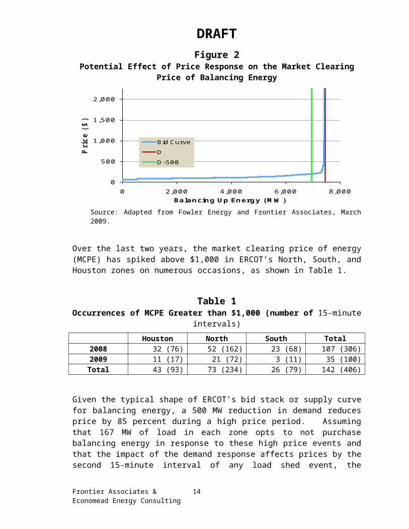
Figure 2 reflects a typical bid stack for ERCOT Balancing Energy Service (BES) market and potential impact on market clearing price resulting from a reduction in demand for electricity.28 24 This estimate is different from an earlier figure indicated in FERC Report on assessment of demand

response and advanced metering that only reflected actual peak reduction in 2007.25 Jay Zarnikau and Ian Hallett. Aggregate industrial energy consumer response to wholesale prices in the

restructured Texas electricity Market. Energy Economics 2008; 30(4): 1798-1808.26 ERCOT Staff. Load Response Survey: Preliminary Results. Presentation to ERCOT’s Demand Side

Working Group. August 10, 2007. 27 Ahmad Faruqui and Stephen S. George, "The value of dynamic pricing," The Electricity Journal, July

2002; Douglas Caves, Kelly Eakin, and Ahmad Faruqui (2000) “Mitigating Price Spikes in Wholesale Markets through Market-Based Pricing in Retail Markets,” The Electricity Journal, April 2000; and Brattle Group, Quantifying Demand Response Benefits in PJM, Prepared for PJM Interconnection and the Mid-Atlantic Distributed Resources Initiative, January 29, 2007.

28 Ibid. p. 42. It should be noted that a price reduction of this magnitude might not be realized if 1) there was inter-zonal congestion and 2) the demand response was “on the wrong side” of the constraint or insufficient to relieve the constraint. Also, the means through which prices are adjusted to recognize the demand response will greatly affect the price reduction. If curtailable loads are “dispatched” through a unit commitment model and their offers to curtail at various strike prices are compared with offers obtained from generators, the savings from demand response could be immediate. If the announced prices are “fixed” and not adjusted to recognize the demand response, the price reduction may not be immediately realized by the market, although the lower level of demand will place downward pressure on prices in later periods as the demand reduction becomes recognized in a short-term load forecast. If the market’s short-term load forecast properly recognizes price elasticity effects to account for demand reduction in the face of a price spike, then this price reduction may be realized immediately – although an elasticity adjustment could negate price response by reducing forecast demand to a level where a price spike would no longer occur. If demand-side resources can be dispatched by the ISO on the basis of offer prices, then the effect of demand reduction upon price can be recognized immediately.

Frontier Associates & 8Economead Energy Consulting

DRAFTFigure 2

Potential Effect of Price Response on the Market Clearing Price of Balancing Energy

0

500

1,000

1,500

2,000

0 2,000 4,000 6,000 8,000

Pric

e ($

)

Balancing Up Energy (MW)

Bid CurveDD-500

Source: Adapted from Fowler Energy and Frontier Associates, March 2009.

Over the last two years, the market clearing price of energy (MCPE) has spiked above $1,000 in ERCOT’s North, South, and Houston zones on numerous occasions, as shown in Table 1.

Table 1Occurrences of MCPE Greater than $1,000 (number of 15-minute intervals)

Houston North South Total2008 32 (76) 52 (162) 23 (68) 107 (306)2009 11 (17) 21 (72) 3 (11) 35 (100)Total 43 (93) 73 (234) 26 (79) 142 (406)

Given the typical shape of ERCOT’s bid stack or supply curve for balancing energy, a 500 MW reduction in demand reduces price by 85 percent during a high price period. Assuming that 167 MW of load in each zone opts to not purchase balancing energy in response to these high price events and that the impact of the demand response affects prices by the second 15-minute interval of any load shed event, the savings to consumers from 500 MW of price responsive demand reduction, as shown for North, South, and Houston zones in Table 2, is about $51 million per year.29

29 Ibid. p. 45. This calculation is based on a method of “moving down the offer stack.” It is assumed that the ISO immediately changes prices to reflect the demand response and avoid selecting more expensive energy offers. To estimate the overall value of demand response, aggregate bid curves (bid stacks) from actual ERCOT data were reconstructed for the 5 days with the highest daily weighted average MCPE between May 1 and July 22 of 2008.

Frontier Associates & 9Economead Energy Consulting

DRAFT

Table 2Savings (by Zone) From 500 MW of Demand Response

Houston North South Total2008 $ 13,008,712 $ 66,893,446 $ 10,068,548 $ 89,970,706 2009 $ 2,148,604 $ 8,710,481 $ 1,676,660 $ 12,535,746 Total $ 15,157,316 $ 75,603,927 $ 11,745,208 $ 102,506,451

Average $ 7,578,658 $ 37,801,964 $ 5,872,604 $ 51,253,226

If the price were adjusted so that the demand response was reflected in the market price in the first 15-minute interval in which the response occurred, the annual savings from 500 MW of demand response would increase to $89.4 million. This savings could be achieved by treating price-responsive loads as a dispatchable resource, or through other means.

It is not presently possible to predict prices in the upcoming nodal market, but if we assume that future prices and bidding behavior bear some resemblance to what has been exhibited in recent years under the zonal market structure, wholesale energy costs might increase somewhere in the neighborhood of $51 million per year if today’s level of demand response to price was lost. Given the uncertainties surrounding price behavior in the nodal market, this might be a very conservative estimate of the value of such a resource.

5 Advance Notice of Prices in the Future Nodal Market

In contrast to the original intention shown by ERCOT stakeholders to maintain the existing price notification of zonal market operation,30 the proposed Nodal Protocols presented to the Commission for approval excluded such capability. Under the nodal market, prices for generators will be set approximately every five minutes and provided instantly to generators via telemetry, although generators will be settled on a 15-minute interval.31 Similarly, as is the case in the zonal market, loads will be settled on 15-minute interval basis. However, the applicable price upon which loads (actually, the REPs and Qualified Scheduling Entities (QSEs) representing such loads) are to be settled will be the load-weighted average of the nodal prices within each Load Zone. Within a normal 15-minute interval, there will be at least three price changes, since ERCOT’s SCED model – the model used to calculate nodal prices -- will be solved at least once every five 30 ERCOT, Market Restructuring: Cost-Benefit Analysis, Final Report, November 30, 2004, Page 6-10,

footnote no. 65. Also available at: http://interchange.puc.state.tx.us/WebApp/Interchange/application/dbapps/filings/pgSearch_Results.asp?TXT_CNTR_NO=28500&TXT_ITEM_NO=28.

31 It is ERCOT’s intention to run SCED at least once every 5 minutes. If nothing happens to the system, a SCED run will be executed by default every 5-minute resulting in Base Points and LMPs. However, certain circumstances, such as major forced outages, may result in a need for SCED run to take place more frequently than the default 5-minute. Such circumstances will cause market to have more than three LMPs within 15-minute settlement interval. These LMPs will be time stamped and properly weighted to generate relevant required settlement prices.

Frontier Associates & 10Economead Energy Consulting

DRAFTminutes. However, since loads are settled on 15-minute interval data and not the zonal-equivalent 5-minute SCED price,32 ERCOT must calculate the load-weighted average of the SCED prices across a 15-minute settlement period in order to generate the settlement price. This step requires both the Locational Marginal Prices (LMPs) from SCED for each node as well as the latest corresponding load level from the State Estimator at each node within a zone. Consumers will therefore not know the actual settlement price until well into the last few minutes of the 15-minute settlement interval.

The fact that load in the nodal market will be settled on a 15-minute interval rather than on a 5-minute SCED interval renders futile any attempt by load to respond to SCED interval prices. For example, if a consumer purchases 1 MWh during the first 5-minute interval when the price is $20 per MWh and completely curtails its purchases during two subsequent 5-minute intervals in which $1000 per MWh was the applicable zonal price, the consumer will pay not $20, but $673.33 This is illustrated in Figure 3.

Figure 3Settlement Cost of Power to the Consumer Should Be $20, Rather than $673

Load Level

Price

t0

$20/MWh $1,000/MWh $1,000/MWh

t0 + 5 minutes t0 + 10 minutes t0 + 15 minutes

1 MWh 0 MWh 0 MWh

Thus, not only is the zonal SCED price signal not received until 30 to 60 seconds after the start of each operating interval, but also, use of a load–weighted average to calculate the zonal 15-minute settlement price means that a load will bear the cost of a high-priced SCED interval even if it drops its consumption as quickly as practical to zero during the SCED interval. This problem of matching consumption to the correct prices could be solved by allowing price responsive loads to be settled on a SCED interval basis.34

However, there would still remain the further problem that loads would be receiving ex-post notice of the zonal SCED price.

Two arguments have been made in support of the elimination of advance notice of RTM prices, neither of which justifies the detrimental consequences of eliminating advance notice. Each will be examined below.

32 Once the 5-minute SCED prices have been calculated, ERCOT can calculate the zonal-equivalent SCED price reflecting the same 5-minute interval and send such information to the Market Information System (MIS) for public posting. While informative, however, such zonal-equivalent SCED price will not be very helpful in assisting consumers to know the 15-minute settlement prices to be used for each Load Zone.

33 $673 = 1 MWh * [($20 + $1000 + $1000) /3].34 This option is further discussed under solutions in Section 7.

Frontier Associates & 11Economead Energy Consulting

DRAFT1. Minimization of load forecast error : The elimination of the advance notice

period was designed to reduce forecasting error, which had led in recent years to reliability problems and an occasional over-commitment of generation resources. It is unreasonable, however, to sacrifice demand response, which is an essential component of a healthy competitive market, for the purpose of reducing forecast error. A far sounder approach is to continue to improve load forecasts while facilitating further price responsive load activities.

ERCOT has proactively taken steps in recent years to improve its load forecast.  A recent presentation to the ERCOT Board of Directors shows significant improvement in day-ahead forecasts (the mid-term load forecast or “MTLF”) over the last couple of years, resulting in the annual Mean Absolute Percentage Error (MAPE) (run at 16:00 p.m. to determine the need for Replacement Reserve Service) declining from 3.55% in 2007 to 2.88% in the first seven months of 2010.  The July 2010 figure was 2.39%.35 Similarly, the MAPE for ERCOT’s short-term load forecast (STLF) used to be less than 1% a few years ago, and much lower errors should be expected given continuous improvements in ERCOT load forecast. In addition, ERCOT has relied on other forecasting services to improve its forecast. In particular, ERCOT relies on a consulting firm (TrueWind) to generate accurate forecasts of wind-powered generation resource production potential and expects wind resources to reflect such forecasts in their resource plans. 

2. Availability of DAM price information : The Day Ahead Market is very useful for some responsive loads with load characteristics well suited for DAM participation. However, participation in DAM is not an effective solution for consumers with fluctuating load levels, like residential consumers and steel mills. These types of loads are not able to reasonably forecast their next-day load levels on an hourly basis. If they do not know what quantities to enter in DAM, it is difficult for them to participate. These customers represent a sizeable percentage of the loads potentially capable of responding to prices. Furthermore, the price information provided in the DAM is not particularly useful to them for the purpose of making effective decisions regarding their actual electricity consumption during real time. As discussed previously, there exists no reasonable expectation of price convergence between the DAM and the RTM given ERCOT’s energy-only market design. Realized prices in the DAM will likely be a poor indicator of RTM prices.

Compared to the current zonal market operation where deployment decisions are delayed by about 30 minutes, the move to nodal operation with more frequent dispatch intervals (5-minutes or less) will result in faster response by the system operator to changes in demand. With the movement from 15-minute to 5-minute dispatch intervals and recent improvements in ERCOT load forecasts, it is anticipated that ERCOT’s operators will have much better information with which

35 Saathoff, K., Grid Operations and Planning Report, a Presentation to the ERCOT Board of Directors on August 17, 2010, Slide 8. Also available at: http://www.ercot.com/content/meetings/board/keydocs/2010/0817/Item_08_-_Grid_Operations_and_Planning_Report.pdf .

Frontier Associates & 12Economead Energy Consulting

DRAFTto make operational decisions. ERCOT’s recent plan to reduce its procurement of Regulation Service following the implementation of the nodal market reflects this consideration.36 Therefore, it is questionable whether the elimination of the notice period for wholesale prices will provide substantial additional gains in operational efficiency.

6 Price Responsive Loads and Price Notice Periods in Other Wholesale Electricity Markets

Other advanced wholesale electricity markets have grappled with the challenge of providing accurate and timely price information to consumers. A survey of some selected markets was conducted to learn more about the way other restructured wholesale electricity markets have addressed advance notice of prices. Three Northern U.S. markets, which are considered the most advanced nodal wholesale electricity markets, along with three foreign electricity markets and the newest nodal operating market in California, were considered. These markets are operated by:

New England ISO (ISO-NE) New York ISO (NYISO) Pennsylvania-Maryland-New Jersey Interconnection (PJM) Australian Electricity Market Operator (AEMO) Alberta Electric System Operator (AESO) (Alberta, Canada) Independent Electricity System Operator (IESO) (Ontario, Canada) California ISO (CAISO)

In U.S. nodal markets, real time locational marginal prices (LMPs) are calculated and announced for each 5-minute operating interval. Load-weighted average LMPs are then calculated representing each market’s settlement interval to be used to settle loads within each Load Zone.

A summary of price notification activities and communication methods in selected wholesale electricity markets is provided in Table 3. NYISO, considered to be one of the world’s most “complete” and advanced wholesale electricity markets, provides prices to consumers five minutes in advance of each settlement interval. Similarly, CAISO, which has been operating under a nodal market design since April 2009, provides pricing updates five minutes before the trade period by announcing prices in its Open Access Same-time Information System (OASIS) as well as on its webpage. Demand resources rely on these prices; however, these prices are not binding. Rather, ex-post prices, which are posted in the CAISO Market Price Interface (CMPI), are used for settlement purposes. In contrast, a number of other markets, including the competitive wholesale markets of Ontario, Alberta, Australia, and New England, provide price forecasts to the market to facilitate demand response.37

36 See presentation by ERCOT staff, John Dumas, titled “2010-2011 Ancillary Service Methodology Workshop”, July 2, 2010. Also available at: http://www.ercot.com/content/meetings/other/keydocs/2010/20100702-ASM/2010-2011%20AS%20Methodology%20Workshop-07022010.pdf .

37 A summary of various characteristics of demand response programs in various wholesale electricity markets is provided by ISO/RTO Council in “North American Wholesale Electricity Demand Response

Frontier Associates & 13Economead Energy Consulting

DRAFTTable 3

Real Time Energy Price Notification in Selected MarketsMarket Advance Notice

of PriceSettlement

IntervalPrice Forecast Communication

(Publicly Available)

ERCOT (Zonal)

Ex-Ante, 10-Minute 15-munute No Website

ISO-NEEx-Post after the end of each 5-minute interval

Hourly Price forecast in Day Ahead for hours during the operating day.

Hourly price forecast in Operating Day two-hour in advance

Website

NYISO Ex-Ante, 5-Minute in advance

Hourly No Website

PJM Ex-Post after the end of each 5-minute interval

Hourly No N/A

AustraliaEx-Post after the end of each 5-minute interval

30-minute Price forecast reflecting various demand scenarios is published every 30 minutes for the next trading day

Website

Alberta AESO

Ex-Post pool price after the end of each operating hour

Hourly Price forecast two hours in advance of each operating hour

Website

Ontario IESOEx-Post, 2 minutes after the end of each 5-minute operating interval

Hourly Hourly price forecasts are provided beginning 36-hours ahead till one hour before operating hour

Website

CAISO Ex-Post after the end of each 5-minute interval

10-minute Non-binding price updates 5-minute before each operating interval

Website

In summary, the need for advance notice of price is widely recognized and addressed in various surveyed wholesale electricity markets using at least one of the following two mechanisms:

Announcing prices (LMPs) several minutes in advance of each operating interval

Providing price forecasts on a frequent basis well in advance of each operating hour

A more detailed review of price responsive load products in some selected wholesale electricity markets is presented in Appendices I and II.

2010 Comparison”, May 2010. Also available at: http://www.isorto.org/site/apps/nlnet/content2.aspx?c=jhKQIZPBImE&b=2613997&ct=8400541&notoc=1.

Frontier Associates & 14Economead Energy Consulting

DRAFT7 Recommended Solutions

In this section, we discuss steps that should be taken to resolve the ex-post pricing problem and effectively integrate price responsive loads into the market, including:

Providing advance notice of settlement prices

Using the SCED interval as the settlement interval for loads that have or are willing to acquire IDRs

Providing informational price forecasts during the Operating Day

Establishing a special economic demand response program based on binding forecasts of prices

Allowing price responsive loads to be modeled directly into the SCED model

These steps are identified to improve load participation and further enhance voluntary load responses to market prices. While some of them are focused on providing advance notice of prices, others are recommended to increase choices to loads. Each of these steps should be implemented by ERCOT to address existing shortcomings in the nodal ERCOT market design that prevent effective price response participation.

7.1 Providing Advance Notice of Settlement Prices

In order to maintain the current zonal level of participation by price responsive loads, ERCOT should introduce a delay between the time that prices are calculated and the time at which the prices would go into effect in its nodal software.

To preserve the current notice period of nearly 10 minutes prior to the complete 15-minute settlement interval, this delay would need to be at least 20 minutes. Using the 1 p.m. to 1:15 p.m. settlement interval as an example, an announcement of prices at 12:50 p.m. of the price at 1:10 p.m. would provide a load or load-serving entity with complete price information for all three operating intervals within the 1:00 p.m. to 1:15 p.m. settlement interval. This assumes that the SCED is not run, and prices are not reset, after 1:10 p.m.

As discussed in the following subsection, a 5-minute notice period may provide a sufficient notice period for many loads. If so, then a 15-minute delay in the period between price announcements and the application of prices would normally suffice.

Implementation of a delay of 10 minutes or less would not be useful because it would effectively provide no advance notice of price. For example, if the price for 1:10 p.m. was announced at 1 p.m., then it would be likely being too late for a load to adjust its demand for the 1 p.m. to 1:05 operating period. And, as noted earlier, the price established for that later 1:10 to 1:15 p.m. period is one-third of the price information used to establish the price in effect from 1 p.m. to 1:05 p.m. settlement interval.

Introducing a delay between the time that prices are calculated and the time at which the prices would go into effect results in LMPs generated by SCED becoming effective five or six five-minute operating intervals later. For example, a SCED result generated at the current time (Interval t) becomes effective for the duration of the upcoming operating

Frontier Associates & 15Economead Energy Consulting

DRAFTinterval that begins twenty minutes later, if the present period of advance notice is to be preserved. As part of this solution, ex-ante price information would be provided publicly and be available to all market players at the same time. For consumers, this is the best solution to the ex-post pricing dilemma, because it maintains the market feature that already exists in the zonal market to enable loads to respond effectively to prices. This would involve the following steps:

Solve SCED for a future period

Calculate zonal prices, based on either a forecast of load for the nodes within each zone or the most recent load information

Provide the 15-minute load zone settlement prices to the market

The advantage of this option is obvious. Price responsive consumers would receive ex-ante pricing with a sufficient amount of advance notice to ensure their ability to adjust their consumption in real-time in response to that price. The consumer’s right to know what the price is before the purchase decision is made is fully assured, which is an essential element of any competitive market.

There may be some periods in which ERCOT’s system operators need to make dispatch decisions closer to real-time, and prices would then be set in real-time during such events. This is particularly evident when ERCOT requires Responsive Reserve Service (RRS) be deployed and should take the energy generated from deployed units into its dispatch decisions. Given the fact that such RRS deployments have taken place a few times during the course of a year in recent years38, it is possible to exclude such intervals from advance notification requirement to address any potential reliability concerns.

The obvious drawback to this approach is that a few minutes of advance notice of price would require ERCOT to rely on load forecasts, rather than solely telemetry or Supervisory Control and Data Acquisition (SCADA) readings, to instruct generators. As is the case today, there would be a gap in the time between 1) setting prices and dispatching instructions, and 2) the period in which the prices would apply. The use of short-term load forecasts rather than real-time information would result in some inaccuracy. It could be alleged that loads would respond to prices and this could result in more need for Regulation. This argument involves four steps:

1. Price spikes lead to “price chasing” by price-responsive loads.

2. Price chasing behavior leads to more deployments of Regulation Down and, perhaps, Regulation Up.

3. The deployments eventually lead to greater obligations of Regulation, since deployments during the previous 30 days are one of the factors considered in setting the schedule of Regulation obligations for the next month.39

4. Higher obligations increase costs to consumers.38 ERCOT has had 11 such events in last three years as indicated in a recent Presentation by ERCOT Staff

at DSWG Meeting on September 2, 2010 titled: Load Participation Update, Slide 6. Also available at: http://www.ercot.com/content/meetings/dswg/keydocs/2010/0910/10--09-10_Load_Participation_Update.pdf .

39 ERCOT, 2010-2011 ERCOT Methodologies for Determining Ancillary Service Requirements, draft of August 2010.

Frontier Associates & 16Economead Energy Consulting

DRAFTAs noted earlier, there is about 600 MW of load that likely to respond to a spike in prices, when adequate notice is provided. Steps 2 and 3 can be statistically analyzed using recent data on ERCOT’s operations.

Hourly data for 2007 and 2008 were examined to test the Step 2 relationship. Very simple comparisons between wholesale prices and deployments are provided in Figures 4 through 6. The relationship between ERCOT’s deployment of Regulation Down and prices – though positive – is very weak, as evidenced by the very low coefficient of determination (R2) statistics.

Figure 4Plot of North Zone Prices vs. Regulation Down Deployments

Frontier Associates & 17Economead Energy Consulting

DRAFT

Figure 5Plot of South Zone Prices vs. Regulation Down Deployments

Figure 6Plot of Houston Zone Prices vs. Regulation Down Deployments

Frontier Associates & 18Economead Energy Consulting

DRAFT

Additional regression models were estimated to discern whether the impacts of wholesale prices on the deployment of Regulation Down could be detected, while controlling for the effects of wind generation and hourly demand on the system. For the three zones examined (North, South, and Houston) these three variables explain less than 1% of the variation in the amount of Regulation Down deployed by ERCOT, as presented in Appendix III. While there is little evidence of a relationship between North Zone prices and Regulation Down deployments after controlling for the effects of wind generation and overall demand, the relationships between wholesale prices in the Houston and South zones were found to be marginally significant. These conclusions hold regardless of whether the price variables are modeled as wholesale prices in dollars or as dummy variables reflecting the presence of a price spikes (using a $300 threshold). Not surprisingly, if a double-logarithmic specification is employed, the statistical results improve. Slightly superior statistical results can be obtained if 15-minute interval data are used and all variables are represented in “change” form. Then, almost three percent of the interval-to-interval variation in Regulation Down deployments can be explained by interval-to-interval variations in wholesale prices during price spikes, load levels, wind generation, and nuclear generation. In conclusion, the step 2 relationship is very weak and many other factors are responsible for the deployments of Regulation Down.

According to the 2010 ERCOT Methodologies for Determining Ancillary Services Requirements, the deployment of Regulation, as well as wind generation, dictates the obligations for Regulation imposed by the ISO on load-serving entities:

Using archived data, ERCOT will calculate the 98.8 percentile of actual Regulation Service deployed hourly for the 30 days prior to the time of the study and the same month of the previous year. In order to consider the increased amount of wind penetration, ERCOT will calculate the increase in installed wind generation capacity and then, depending on the month of the year and the hour of the day, will add incremental MWs to the 98.8 th value.  The tables of Incremental MWs for Regulation Up and Down come from the Appendix of GE’s final report to ERCOT and contain additional MWs for every 1000 MW increase in wind capacity.  The increase in wind capacity will be calculated by taken [sic] the total nameplate capacity of wind resources in the ERCOT network model at the time of the procurement study and subtracting out the total nameplate capacity of wind resources in the ERCOT model at the end of the month being studied from the previous year.

Some simple regression analysis presented in Appendix IV confirms this. Deployments of Regulation Down during one month lead to higher obligations for Regulation Down during the following month, after controlling for the effects of wind generation.

While the empirical evidence needed to support step 2 in this argument appears to be weak, it is nonetheless plausible that running SCED close to real-time, as is planned under nodal operations, may result in some, albeit small, reduction in the need for Regulation. However, no evidence has been presented which purports to link any increase in the need for Regulation with the elimination of advance notice of price.

Frontier Associates & 19Economead Energy Consulting

DRAFTERCOT’s plans to reduce Regulation obligations by 50% are instead tied to other factors.40

Even if some savings in ancillary services costs could be achieved by reducing the response of loads to wholesale price changes, could the cost savings from reduced ancillary services justify the cost of losing demand response to real-time prices? As is depicted in Table 4, if the value of demand response is roughly about $51 million per year41 and the price of Regulation is roughly $12/MW,42 then ERCOT’s use of Regulation would need to be reduced by an average of 485 MW per hour in order to equal the value of the lost demand response. This would be an unreasonably large reduction. Thus, the cost resulting from the elimination of advance notice of price may well surpass any expected potential benefits from reduced Regulation costs that the market may observe from the elimination of advance notice of price under nodal operation.

Table 4Expected Regulation Reduction to Match Benefits from Price

Responsive Demand

Benefits from Price Responsive Demand Reduction $51,000,000Assumed Price of Regulation (per MW per Hour) $12Reduction in Annual Regulation Procurements Necessary to Offset the Value of Demand Reduction (MW)

4,250,000 MW

Reduction in Hourly Regulation Procurements Necessary to Offset the Value of Demand Reduction (MW/h)

485 MW

This question can also be examined by quantifying any increase in the cost of Regulation Down that might possibly be attributable to demand response to prices using the regression models presented in Appendix III and IV. The detailed calculations presented in Appendix VI suggest that if price chasing by energy consumers does indeed lead to greater deployments of Regulation and, ultimately, greater obligations of Regulation, the estimated relationships in Appendix III suggests that this price chasing adds roughly $2 million to the annual cost of Regulation Down.

In conclusion, the benefits to the market of preserving the ability for loads to respond to prices would likely exceed the costs (e.g., the costs of software changes, maintaining

40 It should be noted that ERCOT presently plans to cut its Regulation obligations in half as it moved from 15-minute settlement intervals to (roughly) 5-minute intervals for SCED runs. Under nodal operation it is expected that “More frequent execution of the real-time market should result in less required regulation.” See presentation by ERCOT staff, John Dumas, titled “2010-2011 Ancillary Service Methodology Workshop, July 2, 2010. Also available at: http://www.ercot.com/content/meetings/other/keydocs/2010/20100702-ASM/2010-2011%20AS%20Methodology%20Workshop-07022010.pdf

41 This makes the simplifying assumption that all demand response to prices will be lost if price notice is eliminated. The reader may wish to assume that some loads find a means of responding to DAM prices or reliability indicators.

42 Monthly average Regulation Up prices ranged from $14 to $40 in 2008 and from $5 to $14 in 2009. Regulation Down prices tend to be lower. See 2009 State of the Market Report for the ERCOT Wholesale Electricity Markets, Potomac Economics, July 2010, Figure 21, p. 30.

Frontier Associates & 20Economead Energy Consulting

DRAFTERCOT’s short-term load forecasting system, and, perhaps, some small increased need for Regulation service) that would likely be incurred in preserving advance notice of prices.

It is important to note that advance notice of price does not require the use of a 15-minute settlement interval. With the introduction of advanced metering, most ERCOT loads should be capable of being settled on intervals of 5 minutes or less. The smaller the settlement interval, the less price implementation lag that is required to provide ex-ante pricing.

7.2 Using the SCED interval as the Settlement Interval for Loads That Have or Are Willing to Acquire IDRs

The SCED model generates Locational Marginal Prices (LMPs) for resource nodes as well as all delivery points within ERCOT. Immediately after SCED prices are calculated, ERCOT calculates the zonal SCED price for each load zone. Loads with IDR meters can effectively engage in price response in the ERCOT Nodal market if they are provided advance notice of the zonal SCED price, provided that they are settled using the SCED intervals as settlement intervals. Absent the use of a SCED settlement interval, loads would still be caught in the 15-minute averaging dilemma previously depicted in Figure 3. The use of SCED intervals as opposed to 15-minute intervals to settle loads would result in the ability to provide ex-ante pricing with far less price implementation lag than would be the case using the current 15-minute interval and without the price distortion created by 15-minute averaging.

Under this scenario, loads would receive less advance notice of price than is currently the case in the zonal market. While less than ideal, this nonetheless still preserves the opportunity to respond to price while at the same time avoiding the 15-minute averaging dilemma. In order to have time to process the price data and implement an informed price response, loads would require a minimum of approximately 5-minute advance notice of the zonal SCED price.

Avoidance of the 15-minute averaging dilemma would be viable only for loads possessing the metering capability to capture usage in increments of 5 minutes or less. Large commercial and industrial loads already have that capability, or are able to acquire it on a cost effective basis. Small commercial and residential loads may or may not have that capability, depending upon the capabilities of their advance meters. However, even if small loads must be settled on a 15-minute basis, the advance notice of zonal SCED prices would still be extremely useful to REPs and QSEs wanting to develop and provide demand response programs to those loads. For instance, with advance knowledge of SCED prices, a signal could be sent to advance meters to reduce air-conditioning and other significant loads for short intervals. Thus even without SCED interval settlement, smaller loads could reap substantial cost savings by virtue of this proposal.

Providing the option for SCED interval settlement would not disadvantage other consumers settled on a 15-minute basis. Because the zonal SCED price would be used, there would be no issue of arbitraging between zonal and nodal prices, nor would costs be

Frontier Associates & 21Economead Energy Consulting

DRAFTshifted from one group to another. The policy intent of using zonal average pricing would be fully preserved.

The disadvantage of this proposal, if any, would be the potential impact on ERCOT hardware and software. This would need to be studied by ERCOT. However, it is extremely unlikely that the cost would exceed the benefit of enabling loads to engage in demand response. Similarly, ERCOT would need to examine the software impact of settling loads on a combination of SCED intervals and 15-minute intervals. While moving to 5-minute settlement of load can address the price notification, it is expected to result in “significant” revision and more “complexity” in the ERCOT settlement process.

As previously discussed, the impact of this proposal on required Regulation quantities should be de minimis.

7.3 Providing Informational Price Forecasts During the Operating Day

While non-binding price forecasts are by no means an adequate substitute for ex-ante pricing, they may have some value in encouraging load responses. The real time load response in ISO-NE is based on forecast prices by the ISO. CAISO provides non-binding price updates five minutes before the trade period. Ontario IESO, Alberta, and New York provide some form of non-binding price forecasts for various load zones to enhance economic load responses. As mentioned earlier, ‘advisory’ 15-minute interval zonal LMPs looking 2 ½ hours ahead are provided by NYISO. In addition, Australia, Alberta, and Ontario provide price forecasts in the day-ahead period, covering hours during operating days. Some supplemental price forecasts are also provided close to real time during operating day. Some of these markets extend price forecasting activities into the operating day and provide updates to their forecasts a couple of hours before the actual operating hour. As is the case with wind activities where ERCOT relies on AWS Truewind services to estimate the Wind-powered Generation Resource Production Potential for wind generators, ERCOT can rely on similar forecasting services as CAISO does to publicly provide price forecasts at least 5 minutes in advance of real time. This is a practical, reasonably inexpensive way to encourage more participation by price responsive loads in ERCOT market but is a wholly inadequate stand-alone solution to the ex-post pricing problem.

For consumers, responding to non-binding forecasts of prices would pose a number of risks. Consumers incur costs by responding through shutting down or rescheduling operations. Response to a forecast of a high price that turns out to be false may result in net costs to consumers.

Due to liability concerns over providing price forecasts which may turn out to be inaccurate, ERCOT has expressed little past interest in providing price forecasts. Involving ERCOT in such a role may lead to an uncomfortable level of involvement by ERCOT in affecting actual market prices.

Some have argued that the DAM will provide a reasonable forecast of real-time prices. However, the prices that come out of DAM will be hourly, while real-time prices will change every 15 minutes for QSEs representing load and even more frequently for

Frontier Associates & 22Economead Energy Consulting

DRAFTgenerators. Consequently, DAM prices will reflect a lot of averaging. Also, unexpected events between the day-ahead and real-time will result in a divergence between day-ahead and real-time prices.

Regardless of how the ex-post pricing problem is resolved, ERCOT could and should enhance demand response by preparing price forecasts throughout the Operating Day, preferably in a similar way as CAISO provides pricing updates five minutes before each trade period.

7.4 Establishing a Special Economic Demand Response Program Based on Binding Forecasts of Prices

Establishing a new program through which price responsive loads would be provided binding price forecasts in advance of real time operation would provide a meaningful enhancement of loads’ ability to respond to price, and should be implemented as an additional price responsiveness tool. This is the way IESO in cooperation with Ontario Power Authority handles price responsive loads. Compensation is determined in advance where customers are guaranteed to receive certain payment to encourage load reduction regardless of the actual price in real time. To improve the accuracy of price forecast, binding price forecasts should be announced close to each operating interval providing advance notice ranging from 10-minute to one hour. Detailed requirements for participation in this program, for instance baselines to measure load reduction, are developed to ensure accuracy in measuring load reductions.

At the retail level, a variety of critical peak pricing programs are based upon this same concept. A utility notifies price responsive consumers when a high price is forecast. The program participant is either 1) compensated based on the demand reduction achieved during the peak price period relative to a baseline load level, or 2) pays for its consumption during the peak price period at the forecast price.

Using this approach, decisions would need to be made regarding:

How baseline load levels would be set, if participating loads were to be paid based upon their demand reduction.

How close to the interval would the forecast be released.

How the price information would be conveyed to price-responsive loads.

Another attractive feature of this approach is that the actual real-time price could reflect the demand response. Real-time prices could be reset to lower levels based on the anticipated demand reduction achieved through the program. While the forecast price was binding and fixed upon program participants, the actual real-time price could reflect the anticipated demand response and be set lower. This could be accomplished by adjusting the short term load forecast for the anticipated demand reduction from the program participants (e.g., through an elasticity adjustment).

Frontier Associates & 23Economead Energy Consulting

DRAFT7.5 Allowing Price Responsive Loads to be Modeled Directly in SCED

Model

Many of the markets surveyed in the previous section have programs that permit price responsive loads to be treated as a resource in the optimization process (i.e., SCED or SCUC) and bid into the market. A similar recommendation is included in a study recently commissioned by ERCOT to assess the risks of moving to a nodal market.43

Such capability provides responsive loads the means to effectuate an informed economic decision regarding their electricity consumption.

Permitting price responsive loads to submit offers for load reduction or interruption and modeling those loads directly in SCED would provide substantial benefits to the market and maximize potential demand response within ERCOT. It would effectively place both generators and price-responsive loads on an equal footing in balancing the supply/demand equation. Although ex-ante pricing is not provided if this option alone were undertaken, it would protect price responsive loads from price spikes because each load would designate the price point at which it chooses to interrupt rather than consume. Furthermore, paying participating loads the market clearing price for their load reductions appropriately compensates loads for their contribution to lowered system costs. Because actual demand response is modeled in real-time through SCED, the impact on market-clearing prices is immediate.

There are at least two concerns that surface with this option. First, modeling loads in SCED is an extremely complex undertaking. Of all of the solutions discussed in this paper, this approach would be by far the most difficult to implement. The ERCOT staff is presently preparing an analysis of the impact this approach would have on ERCOT systems. At such time as that analysis is completed, the feasibility of pursuing this approach should be more apparent.

The second concern pertains to the potential requirements imposed on loads desiring to participate in SCED. None of those are presently known and will have to be worked out if and when the details of this proposal are flushed out. It is incumbent upon policy makers to ensure the broadest possible participation by divergent types of loads. Were this option to be implemented, any price-responsive loads incapable of participating in SCED would be effectively denied their right to advance notice of price in the RTM, unless an option providing ex-ante pricing were also implemented. For this reason, the options of load participation in SCED and the provisioning of ex-ante pricing should be viewed as complimentary rather than substitutable.

43 Market Reform, “Nodal Protocols Risk Assessment, Phase 1: Overall Assessment, Identification of Material Risks,” Presentation to NATF, August 31, 2010, Slides 28 and 29.

Frontier Associates & 24Economead Energy Consulting

DRAFT

Appendix I: Price Responsive Loads in Selected Wholesale Electricity Markets

A survey of some selected markets was conducted to learn more about their price responsive load activities. The following wholesale electricity markets were included in the survey:

New England ISO (ISO-NE) New York ISO (NYISO) Pennsylvania-Maryland-New Jersey Interconnection (PJM) Australian Electricity Market Operator (AEMO) Alberta Electric System Operator (AESO) (Alberta, Canada) Independent Electricity System Operator (IESO) (Ontario, Canada) California ISO (CAISO)

The following paragraphs provide a summary of price responsive load programs within each wholesale electricity market. For more details regarding these programs, please see information provided in Attachment II.

1. New England Electricity Market

The market served by the New England Independent System Operator (ISO-NE) has a nodal structure, featuring a Day Ahead Market (DAM) and a Real Time Market (RTM) for energy and RTM for ancillary services. The DAM is settled on an hourly basis, while the RTM is settled hourly based on weighted average of twelve 5-minute dispatch interval prices. ISO-NE loads are settled at 8 load zones, one for each state, with Massachusetts representing 3 zones. The load-zone price is the average of the nodal prices within the zone.44 ISO-NE issues an hourly price forecast in the DAM for the next operating day. In addition, an advanced hourly price forecast is released for the remaining hours of the current operating day every other hour. The actual spot price is calculated after the fact (ex-post), and publicly announced at the end of each 5-minute interval. Before the fact (ex-ante) pricing is not emphasized because the region does not support the industrial load that might request advanced price notification.45

ISO-NE used to operate several price responsive programs; however, all capacity related price responsive loads were incorporated into ISO-NE Forward Capacity Market (FCM) program effective June 1, 2010.46 Currently, ISO-NE operates two programs a) Day-Ahead Load Response (DALR) and b) Real Time Price Response.

a. ISO-NE Day-Ahead Load Response Program

The Day-Ahead Load Response Program allows participants to make energy reduction offers concurrent with the DAM. Participants submit an offer to ISO-NE, specifying price, amount of

44 ISO New England, “2009 Annual Markets Report,” Internal Market Monitor, May 18, 2010, page 28.45 Conversation with Dr. Mario Depillis and Henry Yoshimura, July 19, 2010.46 Conversation with Dr. Mario Depillis and Henry Yoshimura, July 19, 2010.Frontier Associates &

Appendix I-1Economead Energy Consulting

DRAFT

curtailment, minimum duration and an optional start-up/shut-down cost at which they are willing to reduce their consumption for the following day. The offer is compared with the DAM hourly clearing prices in their load zone. If the combination of the customer’s price and the optional start-up/shut-down cost is less than or equal to the DAM hourly clearing price, the offer is accepted.47 If the participants do not curtail consumption when scheduled, they are charged the difference between actual reduction and the reduction offered at the hourly Real-Time locational marginal price (LMP) in the load zone. If loads reduce consumption at a greater amount than offered, they will be paid the difference. 48

b. ISO-NE Real Time Price Responsive Program

In ISO-NE’s Real Time Price Response Program, participants are notified when wholesale prices in their region are forecasted to exceed $0.10 per kWh in any hour during the next day.49

Any voluntary reduction in electricity consumption a participant makes during these designated program hours is eligible for incentive payments, and there is no penalty for failing to curtail consumption. Participants are paid the greater of the wholesale electricity price in the region or a minimum of $0.10 per kWh. Communication that an eligibility period is open is made through e-mail notification the night before or in the morning of a price event and is posted on the ISO's web site. Participants must have an electric meter capable of recording the building’s electricity consumption every hour (an interval or hourly meter).50

2. New York Independent System Operator Market

The New York Independent System Operator (NYISO) administers markets for installed capacity, energy, ancillary services and transmission congestion rights. NYISO runs both a Day Ahead Market (DAM) and a Real Time Market (RTM) and is designed as a nodal market. The Day Ahead Market runs a Security Constraint Unit Commitment (SCUC) algorithm to optimize both energy and ancillary service bids and generates hourly day-ahead Location Based Marginal Prices (LBMP). There is a price cap for both generator offers as well as demand bids currently at $1000/MWh. The Day Ahead LBMPs along with the commitment schedules are posted at 11:00 am day ahead51.

The real time market uses a two settlement process: Real Time Commitment (RTC) and Real Time Dispatch (RTD). RTC runs a SCUC every 15 minutes (considering a 2 ½ hour window) and generates binding unit commitment decisions 45 minutes before the operating hour. RTD runs a Security Constraint Economic Dispatch (SCED) algorithm every 5 minutes. It generates real time LBMPs (both bus level and zone level) and dispatch instructions five minutes ahead 47 ISO New England Inc., FERC Electric Tariff No. 3, Section III – Market Rule 1 – Standard Market Design,

Appendix E – Load Response Program, page 7609-7611, December 2004.48 ISO New England Inc., Demand Response: Frequently Asked Questions: Day Ahead Option, available at:

http://www.iso-ne.com/genrtion_resrcs/dr/broch_tools/da_option_faq.pdf .49 ISO-NE, “2009 Annual Markets Report,” Internal Market Monitor, May 18, 2010, page 49.50 ISO New England Inc., Demand Response: Frequently Asked Questions: Real Time Price Response Program,

available at: http://www.iso-ne.com/genrtion_resrcs/dr/broch_tools/rt_pric_prog_faq.pdf .51 “NYISO Market Participants User’s Guide”, NYISO, February 2010, p. 37-38, 41, and 48.Frontier Associates &

Appendix I-2Economead Energy Consulting

DRAFT

of the interval (ex-ante pricing)52. Price data is publicly available on the ISO’s website. The load is settled based on zonal LBMPs (load weighted average in each of the 11 zones).

NYISO runs two economic load response programs: the Day-Ahead Demand Response Program (DADRP) and the Demand-Side Ancillary Service Program (DSASP).

a. NYISO Day-Ahead Demand Response Program

In DADRP, load has to bid into the day ahead energy market with information about the time duration, reduction in consumption (energy) from a baseline (called the Customer Baseline Load or CBL) and the price (bus level LBMP) at which load is willing to curtail. The minimum price bid is currently $75/MWh, and the minimum load participation is 1 MW53. Generally, interval meters are required for participation in DADRP. The load is treated similar to a generator in the SCUC and is ‘scheduled’ for the next day. The load is paid the hourly bus level LBMP for any energy reduction from the CBL. The part of scheduled energy that is not reduced is charged at the higher of the day ahead or real time LBMP.

b. NYISO Demand-Side Ancillary Service Program

In DSASP, loads of minimum 1 MW capacity with revenue-grade interval billing meters and instantaneous two-way communication meters (telemetry) can bid into both the Day Ahead and Real Time Ancillary Services Markets (operating reserves and regulation service). DSASP resources must qualify through resource testing requirements. The compensation paid is the reserve market clearing price when cleared. Performance indices for DSASP resources are calculated on an interval basis. Non-compliance is measured based on performance indices which are calculated on an interval basis for both Reserves and Regulation. Payment is adjusted by the performance index for the service provided. As of December 31, 2009 there are no resources qualified in the DSASP.54

3. Pennsylvania-New Jersey-Maryland Interconnection Market

Pennsylvania-New-Jersey-Maryland (PJM) Interconnection operates both a Day Ahead Market and a Real Time (or Balancing) Market in energy and ancillary services. Ancillary services currently include operating reserves, but not regulation service.55 It has a nodal market design and generation resources are settled at nodes. Loads are settled at zones that coincide with 17 existing Transmission and Distribution Service Providers (TDSPs) territories.

In the Day Ahead Market, hourly Locational Marginal Prices (LMPs) and hourly commitment schedules for the next day are calculated by simultaneously optimizing for minimum cost for

52 Email conversation with Donna Pratt, Demand Response Market Product Specialist, NYISO, August 10, 2010.53 Presentation on NYISO’s Demand Response Programs, Donna Pratt, November 2009.54 NYISO filing to FERC on Demand Response Programs, January 15, 2010, p. I-2 and I-3. Also available at:

http://www.nyiso.com/public/webdocs/documents/regulatory/filings/2010/01/ICAP_Report_1_15_10.pdf 55 Conversation with Dr. Joe Bowring, PJM Independent Market Monitor, August 4, 2010.Frontier Associates &

Appendix I-3Economead Energy Consulting

DRAFT

energy and operating reserves (Security Constrained Unit Commitment). There is a price cap for both generator offers as well as demand bids currently at $ 1000/MWh. The hourly day ahead LMPs and schedules are posted at 4:00 pm for the next day and are financially binding.

In the Real Time Market, SCED is run every 5 minutes to provide dispatch instructions. The real time LMPs are calculated ex-post (after the fact) and announced at the end of each 5-minute interval. The generators are settled on the hourly average nodal LMPs and loads are settled on hourly averaged zonal LMPs that are calculated based on twelve 5-minute interval prices after each hour.56 The real time prices are available for public access on the website.

PJM’s economic load response program (ELRP) is energy-only. Loads can participate in the ELRP in three ways: submitting an offer in the Day Ahead Market that clears, submitting an offer into the Real Time Market that clears, or self-scheduling load reductions while notifying PJM.57 Participating loads need to have interval metering.

a. PJM Day Ahead Economic Load Response

Demand resources, except those that are charged rates based on real time hourly LMPs, can participate in the Day Ahead Market. Aggregators or Curtailment Service Providers (CSPs) can submit incremental offer curves in minimum increments of 100 kW. All day-ahead load response bids should be submitted by the Day Ahead Market deadline at noon each day. The cleared load response bids will be posted to eMKT (online tool for participants only) at 16:00 along with other Day Ahead Market clearing results. CSPs with loads cleared in the Day Ahead Market are paid the zonal LMP less the generation component of retail rate (customer’s electric bill). Cleared loads in the Day Ahead Market are obligated to curtail during the scheduled hours. The shortfall in performance (reduction) is charged at real time LMP in addition to the balancing operating reserves charges.58

b. PJM Real Time Economic Load Response

In the Real Time Market, the load reduction is voluntary whether it is dispatched by PJM or self scheduled, and therefore there are no penalties for non-compliance. The load is compensated the same way as day ahead scheduled loads for real time performance.

4. Australian National Electricity Market

The market administered by the Australian Energy Market Operator (AEMO) can be considered zonal, with prices settled on the basis of a regional reference price (RRP). There are five RRP zone areas in Australia (South Australia, New South Wales, Tasmania, Queensland and Victoria), operating within a Real Time Market (RTM) for energy and ancillary services.

56 “PJM Manual 11: Energy & Ancillary Services Market Operations”, June 23, 2010, p.47.57 “2009 State of the Market Report for PJM”, Monitoring Analytics, March 2010, p. 10458 “PJM Demand Side Response”, PJM State & Member Training Department presentation, June 2010, Slides 9-

17.Frontier Associates &

Appendix I-4Economead Energy Consulting

DRAFT

While AEMO does not announce prices ex-ante, the entity publishes non-binding 30-minute forecast prices 15 hours in advance of the trading day, which occurs from 4:01 am to 4:00 am the next day and contains 48 trading intervals each lasting for 30 minutes. It also publishes 5-minute forecast prices one hour in advance.59 All of this information is publically available from the ISO's website, and appears on the website soon after the publication to the market.60

A regional dispatch price for energy and ancillary services is calculated by AEMO at its regional reference node using prices from dispatch offers or demand bids submitted into the pool for scheduled generating or loads units, respectively. The dispatch price is determined at the end of each 5-minute dispatch interval. This price is determined by the highest priced resource which is dispatched or allocated to meet demand from the region and is adjusted for electrical losses on the network. For a region, the spot price for a half hour trading interval is calculated as the average of the dispatch prices for each of the six 5-minute dispatch intervals.61

a. AEMO Price Responsive Loads

AEMO allows both large and small loads in the energy, ancillary services, and other emergency services to participate as price responsive loads to avoid the peaks of high spot prices.62 While the mechanism for participation varies, large customers may enter into specific contracts with retailers, who can direct the load to shed when required. The market operator may also take on this role. Price responsive loads are settled on the basis of the real-time RRP, available publicly on AEMO’s website. The incentive for load response is financial, and large customers may directly respond to prices or may enter an agreement where they receive compensation for load shedding.  There are no penalties assessed for loads that fail to conform with pledged reductions.63

5. Alberta Electricity System Operator Market – Alberta, Canada

Alberta Electricity System Operator (AESO) administers only real time energy and ancillary services markets. There is no nodal or zonal design; rather, it is a system wide dispatch market. The market is designed to generate a System Marginal Price (SMP) for energy and dispatch instructions every minute and an hourly system wide (pool) price is calculated after the fact (ex-post) as the time weighted average of the SMPs.64 Operating reserves are also indexed to

59 “An Introduction to Australia’s National Electricity Market,” AEMO, July 2010, p. 12. Also available at: http://www.aemo.com.au/corporate/0000-0262.pdf .

60 Communication with Peter Adams in the Australian Energy Regulator (AER) and his responses to RTO-ISO Questionnaire, August 6 and 18, 2010.

61 National Energy Market, “Settlement Process,” AEMO, 2009, p. 4-5.62 Communication with Peter Adams in the Australian Energy Regulator (AER) and “An Introduction to

Australia’s National Electricity Market,” AEMO, June 2010, p. 13. Also available at: http://www.aemo.com.au/corporate/0000-0262.pdf .

63 Communication with Peter Adams in the Australian Energy Regulator (AER) and his responses to RTO-ISO Questionnaire, August 6 and 18, 2010.

64 “Determining the Wholesale Market Price for Electricity”, AESO, September 2006.Frontier Associates &

Appendix I-5Economead Energy Consulting

DRAFT

this pool price. The hourly pool price is the uniform price applied to both generators as well as loads.65

a. AESO Price Responsive Loads

The AESO currently does not sponsor any programs for price responsive loads, but it releases price forecasts for a two-hour time frame based on latest available data on offers and forecast load. Price responsive loads use these forecast prices to make curtailment decisions. AESO factors in the possible impacts of this demand response (usually about 200-300 MW based on the price) at high forecast prices in short term adequacy calculations.

6. Independent Electricity System Operator Market – Ontario, Canada

The Independent Electricity System Operator (IESO) does not run a Day Ahead Market but there is a Day Ahead Commitment Process (DACP). It allows for the commitment of some generators in the day-ahead time frame in return for financial guarantee. DACP process requires ‘dispatchable’ generators and ‘dispatchable’ loads to submit dispatch data that reflects expected conditions by 11:00 on the pre dispatch day. Dispatchable generators or loads are those that submit bids and offers into the market.66 The commitment is for energy only and is run to address reliability concerns.

The Real Time Market runs a balancing model every 5 minutes to generate real time LMPs and send dispatch instructions to dispatchable generators and loads. The offers and bids from both the dispatchable generators and loads are included in the optimization model. The price is announced 2 minutes after the end of the 5-minut interval (ex-post) on the IESO’s website.67

The 5-minute market clearing prices are averaged every hour into a unified price and the Hourly Ontario Energy Price (HOEP) is charged to non-dispatchable generators and loads. Non-dispatchable generators and loads are those that participate in the market but do not submit bids or offers into the market. Most generators -- but very few loads -- are dispatchable.68

a. IESO Load Response Loads

Dispatchable loads should have the ability to vary their consumption based on the instructions from the IESO every 5 minutes. They have to bid into the market to be allowed to draw power from the grid. They are expected to keep dispatch data up-to-date with their ability to consume. The performance of the dispatchable load is measured within a tolerance level of the dispatch instructions sent.69 There are no additional special incentives offered for loads to participate in

65 Written responses to questionnaire by Dr. Mike Nozdryn-Plotnicki, AESO, July 19, 2010.66 “Day-Ahead Commitment Process - Operations and Settlement Market Manual’, Ontario IESO, December 9,

2009.67 Real time price data is available at http://reports.ieso.ca/public/RealtimeMktPrice/ .68 Phone interview with Andy He and Pat Kamstra, Ontario IESO, July 16, 2010.69 “Overview of the IESO-Administered Markets”, IESO Marketplace training publication, July 2010.Frontier Associates &

Appendix I-6Economead Energy Consulting

DRAFT

the market. Currently there is about 800 MW of dispatchable load in the Ontario IESO territory. Non compliant incidents are taken up and penalties assessed case by case.

b. IESO Price Forecast

The Hourly Ontario Energy Price (HOEP) is calculated after each hour based on the actual consumption during that hour, but the IESO releases a number of price estimates in advance. These forecasts of the HOEP can be used by price responsive loads to adjust their consumption to avoid high prices.

Day Ahead Price Forecast : The day-ahead price forecast is released each day at 17:00 for hourly prices the next day for Monday through Friday. It is based on publicly available data and also includes 95 percent confidence bands.Day Ahead Pre-dispatch Price: The price is calculated with the data from Day Ahead Commitment Process (DACP) using a pre-dispatch algorithm. The process is run every hour starting at 11:00 on the pre dispatch day and the prices are released about 10-20 minutes later. It is based on the offers submitted into the DACP and IESO’s load forecast.Operating Day Pre-dispatch Prices: The pre-dispatch algorithm is also run on the ‘dispatch day’ every hour and generates hourly prices for the entire day. The pre-dispatch price data is available online on the IESO’s website. It is projected based on the latest available supplier offers and load forecast, so it can vary as offers and demand are updated.

7. California Independent System Operator Market

In April 2009 the California Independent System Operator (CAISO) implemented a comprehensive redesign. It now operates a DAM and RTM, both of which serve capacity and energy, an Ancillary Services Market serving capacity, and a Congestion Revenue Rights Market. Loads are settled using load aggregation points, which represent aggregations of individual load nodes. The three major load aggregation points in the system correspond to the service territories of the state’s three major investor owned utilities: Pacific Gas and Electric, Southern California Edison, and San Diego Gas and Electric.70

The Real-Time Market design includes two sequential steps: first, an hour-ahead scheduling process is used to pre-dispatch non-dynamic imports or exports on interties about 45 minutes prior to the start of each operating hour. Second, the real-time dispatch is used to dispatch resources within the ISO and dynamic imports and exports during each 5-minute interval within each operating hour.71 The DAM closes one day before the trade date, with hourly results published by 1:00 pm scheduled at the LMP. The RTM opens at 1:00 pm, when DAM results are published. Real-Time Unit Commitment occurs every 15 minutes, and Real-Time Economic Dispatch occurs every 5 minutes, settled in 10-minute increments based on average 70 California ISO, Department of Market Monitoring, 2009 Annual Report: Market Issues and Performance, April

2010, pages 1.1 to 1.2.71 Ibid, pages 1.5 and 2.7.Frontier Associates &

Appendix I-7Economead Energy Consulting

DRAFT

of 2 five-minute intervals.72 The ISO provides pricing updates 5 minutes before the trade period in its Open Access Same-time Information System (OASIS) or market participants can see price information at CAISO webpage. Demand resources rely on these prices; however, these prices are not binding. Rather, ex-post prices, which are posted in the CAISO Market Price Interface (CMPI), are used for settlement purposes.73

CAISO offers two Demand Response products: Participating Load and Proxy Demand Response.

a. Participating Load Program

Entities within the Participating Load (PL) program (primarily the large pumps installed in public water projects) provide demand responses that can be curtailed according to CAISO needs in the Real-Time dispatch. PL participants can take part in the DAM and RTM. An independent Scheduling Coordinator (SC) is required to represent each curtailable load, and may offer their product to CAISO. Participating Loads do not use a base-line energy calculation to determine the amount of energy curtailed. To qualify for the PL program, a demand response provider must be directly dispatchable and must meet specific telemetry and metering requirements in order to provide ancillary services.74

b. Proxy Demand Response

Introduced on August 10, 2010, the Proxy Demand Response (PDR) program allows demand response providers to offer load reductions as a demand-side resource in the market.75 PDR participants are a load or an aggregation of loads that are capable of verifiably and measurably reducing their electric demand.76 The minimum load size for a Proxy Demand Resource is 0.1 MW (100 kW). PDRs can submit bids into the wholesale Day Ahead and/or Real Time market and respond to dispatches at the direction of the CAISO. The PDR enables integration of retail price responsive demand response programs into wholesale markets. PDR allows customer loads to participate in the CAISO markets by bidding their demand responsive loads into the Day Ahead market, Residual Unit Commitment (RUC), Real Time energy, and Non Spinning Reserve Ancillary Service. CAISO requires that the end use customers have interval meters that meet the Local Regulatory Authorities’ requirements.77 PDR resources are paid for load reductions based on nodal prices where demand reductions occur, rather than based on prices

72 California ISO, CAISO Markets: Real-Time Market Overview, Training Module.73 Written responses to questions by Tom Cuccia, CAISO, September 7, 2010. Advance notice of prices is

available at: http://oasis.caiso.com/mrtu-oasis/?doframe=true&serverurl=http%3a%2f%2ffrptp09%2eoa%2ecaiso%2ecom%3a8000&volume=OASIS

74 California ISO, Demand Response: Frequently Asked Questions, January 1, 2010, pp. 1-2. Also available at: http://www.caiso.com/271e/271ee8df2c760.pdf .

75 CAISO News Release on August 10, 2010. Also available at: http://www.caiso.com/27ee/27ee8c8437f90.pdf. 76 CAISO, 2009 Annual Report, page 18.77 California ISO, Demand Response: Frequently Asked Questions, January 1, 2010, pp. 1-6. Also available at:

http://www.caiso.com/271e/271ee8df2c760.pdf . Frontier Associates &

Appendix I-8Economead Energy Consulting

DRAFT

for much broader load aggregation points used to settle load.78 Penalties are set forth in Section 2.5.26 of the ISO Tariff subject to FERC approval. As was mentioned earlier, PDR is a newly established program for price responsive loads and is expected to go through refinements based on actual performance.79

78 California ISO, “Draft Final Proposal for the Design of Proxy Demand Resource, August 28, 2009, pp. 27-30.79 Additional information on the Proxy Demand Resource product is provided at:

http://www.caiso.com/23bc/23bc873456980.html .Frontier Associates &

Appendix I-9Economead Energy Consulting

DRAFT

Appendix II: RTO/ISO Price Responsive Load Programs (Baseline and Performance)

Price Responsive Load ProgramsU.S. Wholesale Electricity Market Comparison

Demand Response (DR) programs have received increasing attention in recent years and wholesale electricity market operators are integrating more DRs in their day-to-day activities, particularly in markets which are facing declining reserves or are concerned about environmental impacts of generating electricity by their conventional generation resources. Various Demand Response programs are introduced into these markets, baseline figures are calculated to measure DR performance, and financial penalties are imposed for non-compliance with program required performance for some of these Demand Response programs.

Demand Response ProgramsDemand Response (DR) programs are relied upon by market operators to address the need for energy (MWh), capacity (MW), or being used to manage emergency situations either to supplement Operating Reserves or minimizing non-voluntary load shedding. Demand response Programs fall into the followings two major categories:

1. Reliability-based programs

2. Economic-based programs

Customer Baseline LoadCustomer Baseline Load (CBL) is a benchmark against which Demand Response by customers is measured. CBL reflects an estimation of the amount of energy use expected by a particular customer in the absence of load curtailment. Various markets have different formulas to calculate CBL. In general, CBL is based on some historical load level by customers. CBL is either defined universally by a central authority, such as Independent System Operators (ISOs) or is left to customers to provide alternatives calculation subject to certain conditions.

For example, PJM relies on the following CBL for its Economic Load Response for events that take place during weekdays:

The CBL for weekdays shall be the average of the highest 4 out of the 5 most recent highest load weekdays in the 45 calendar day period preceding the relevant load reduction event.

An Interested Party may propose an alternative CBL calculation that more accurately reflects the relevant end-use customer’s consumption pattern. Any such proposal will become effective if agreed by all Interested Parties. In the absence of

Frontier Associates & Appendix II-Economead Energy Consulting

DRAFT

agreement, market operator will establish a CBL which shall be binding upon all Interested Parties.

Calculation of CBL may differ by program. For example, New York Independent System Operator (NYISO) relies on the following CBLs for various products:

Energy: Highest five consumption days of last ten “like” days where DR event or schedule did not occur

Capacity: Average of highest four peak demands in same season (Summer/Winter) of previous year

Real-time: Base load at beginning of a real-time schedule

Non-Compliance PenaltyDepending on the Demand Response programs, there may be some financial consequences if a participant underperforms its obligation. For example, NYISO does not impose any penalty for its Emergency Demand Response Program (EDRP), which is a voluntary program. In contrast, there is penalty for nonperformance for the other two programs, The Day-Ahead Demand Response Program (DADRP) and Installed Capacity Special Case Resources Program (ICAP/SCR). Alternatively, the Electric Reliability Council of Texas (ERCOT) has penalty for nonperformance for its Emergency Interruptible Load Service (EILS) as well as for its Load acting as Resource (LaaR) in the Ancillary Service market when LaaR fails to meet its obligation to provide Responsive Reserve.

The following table provides a summary of various programs, their Customer Baseline Loads, and potential penalties if applicable.

Frontier Associates & Appendix II-Economead Energy Consulting

DRAFT

Baseline and Performance

Price Responsive Load ProgramsU.S. Wholesale Electricity Market Comparison

Market Existing Product Minimum Load

Capacity Payment and Resource Adequacy (RA)

Metering Baseline Customer Baseline Load (CBL)

ISO-NE Real Time Price Response (RTPR)

Day Ahead Load Response

Minimum of 100 KW

Standby generation is included. Minimum of 100 KW

No Capacity payment

Reliability Participants (During Reliability Event) eligible for ICAP credit

No need for Interval Metering

The same

Baseline Calculation

Baseline Calculation

Baseline Calculation with no penalty

No penalty, however, deviations are settled at the real time price

NYISO Day-Ahead Demand Response Program (DADRP) through Customer Bidding with 2-hour Notification (319 MW as of May 2008)

Standby generation is excluded. Minimum 1.0 MW

No capacity payment

Interval Billing Metering

CBL Customer Baseline Load (CBL, a statistical estimation) is based on historical consumption and deviations are settled at the higher of day ahead or real time LBMP. Non-compliance penalty is to charge the higher of Real-Time or Day-Ahead LBMP for load reduction scheduled but not curtailed

PJM Economic Load Response Program (can participate in both Day Ahead and Real-time Markets) (2,944 MW, 608,745 MWH ,and more than $45 million credit in 2007)

No capacity payment

Interval Metering Customer Baseline Load (CBL) or Alternative

Customer Baseline Load (CBL) or Alternative reflecting historical consumption with deficiencies settled at real time prices plus operating reserves

Frontier Associates &Appendix II-3

Economead Energy Consulting

DRAFT

Market Existing Product Minimum Load

Capacity Payment and Resource Adequacy (RA)

Metering Baseline Customer Baseline Load (CBL)

CAISO Participating Load (PL) to be considered as Dispatchable Demand Resource (DDR)

Proxy Demand Response (PDR) is a new program under consideration

Some of the IOUs’ DRs, such as Capacity Bidding Program, will be integrated into MRTU market after successful pilot testing in the near future.

Minimum of 100 KW with Participating Loads at or above 1 MW eligible to participate in ancillary services (Non-Spinning Reserve and Replacement Reserve) and Supplemental Energy markets.

None, unless being considered for ancillary services.

Real-Time Metering (Revenue meter or equivalent subject to prior ISO approval) to provide instantaneous operational data. In addition, telemetry is required to provide ancillary services.

Real-time Performance

Penalties are set forth in Section 2.5.26 of the ISO Tariff subject to FERC approval.

The participant will be treated like any other resource that does not meet their obligation (imbalanced energy).

Frontier Associates &Appendix II-4

Economead Energy Consulting

DRAFT

Appendix III: Regression Statistics for Relationship between Wholesale Prices and Deployments of Regulation

III.1. Relationship between North Zone Prices and Regulation Down Deployments after controlling for the effects for Wind Generation and Hourly Load (data for 2007 and 2008)

Regression StatisticsMultiple R 0.073711389R Square 0.005433369Adjusted R Square 0.005193984Standard Error 1608.415248Observations 12468

ANOVAdf SS MS F Significance F

Regression 3 176152623 58717540.99 22.69715882 1.19657E-14Residual 12464 32244363129 2586999.609Total 12467 32420515752

Coefficients Standard Error t Stat P-value Lower 95% Upper 95% Lower 95.0% Upper 95.0%Intercept 888.0676897 77.53466174 11.45381523 3.18686E-30 736.0877908 1040.047589 736.0877908 1040.047589MCP north zone hourly 0.191324757 0.138982993 1.376605527 0.168658968 -0.081103352 0.463752865 -0.081103352 0.463752865Generation (mwh) wind 0.04733186 0.014898426 3.176970416 0.001491852 0.018128646 0.076535074 0.018128646 0.076535074hourly load 0.015238787 0.002095383 7.272553631 3.73838E-13 0.011131513 0.019346062 0.011131513 0.019346062

Frontier Associates &Appendix III-1

Economead Energy Consulting

DRAFT

III.2. Relationship between South Zone Prices and Regulation Down Deployments after controlling for the effects for Wind Generation and Hourly Load (data for 2007 and 2008)

Regression StatisticsMultiple R 0.079892465R Square 0.006382806Adjusted R Square 0.006143649Standard Error 1607.647349Observations 12468

ANOVAdf SS MS F Significance F

Regression 3 206933863.7 68977954.58 26.6887808 3.36547E-17Residual 12464 32213581889 2584529.997Total 12467 32420515752

Coefficients Standard Error t Stat P-value Lower 95% Upper 95% Lower 95.0% Upper 95.0%Intercept 856.265193 76.80514463 11.14853956 9.95187E-29 705.7152602 1006.815126 705.7152602 1006.815126MCP south zone hourly 0.79961279 0.21519664 3.715730836 0.000203503 0.377794176 1.221431404 0.377794176 1.221431404Generation (mwh) wind 0.062351493 0.015296013 4.076323122 4.60373E-05 0.032368947 0.09233404 0.032368947 0.09233404hourly load 0.014758773 0.002051084 7.195597283 6.57486E-13 0.010738333 0.018779214 0.010738333 0.018779214

Frontier Associates &Appendix III-2

Economead Energy Consulting

DRAFT

III.3. Relationship between Houston Zone Prices and Regulation Down Deployments after controlling for the effects for Wind Generation and Hourly Load (data for 2007 and 2008)

Regression StatisticsMultiple R 0.08163311R Square 0.006663965Adjusted R Square 0.006424876Standard Error 1607.419879Observations 12468

ANOVAdf SS MS F Significance F

Regression 3 216049173.5 72016391.15 27.8722921 5.89148E-18Residual 12464 32204466579 2583798.666Total 12467 32420515752

Coefficients Standard Error t Stat P-value Lower 95% Upper 95%Intercept 889.7821031 76.77942201 11.5888096 6.76172E-31 739.2825907 1040.281616MCP houston zone hourly 1.05282055 0.252842109 4.163944653 3.14901E-05 0.557211007 1.548430092Generation (mwh) wind 0.050392279 0.014856794 3.39186768 0.000696337 0.021270671 0.079513887hourly load 0.013699687 0.002096989 6.533026741 6.69598E-11 0.009589264 0.017810109

Frontier Associates &Appendix III-3

Economead Energy Consulting

DRAFT

III.4. Relationship between North Zone Price Spikes (MCPE > $300/MWh) and Regulation Down Deployments after controlling for the effects for Wind Generation and Hourly Load (data for 1/1/07 to 6/4/08)

SUMMARY OUTPUT

Regression StatisticsMultiple R 0.073662202R Square 0.00542612Adjusted R Square 0.005186733Standard Error 1608.421109Observations 12468

ANOVAdf SS MS F Significance F

Regression 3 175917607.8 58639202.61 22.66671205 1.25136E-14Residual 12464 32244598144 2587018.465Total 12467 32420515752

Coefficients Standard Error t Stat P-value Lower 95% Upper 95% Lower 95.0% Upper 95.0%Intercept (Reg Down Deployment) 886.6010682 77.42136153 11.45163364 3.26725E-30 734.8432552 1038.358881 734.8432552 1038.358881MCP north price greater than $300 195.1264095 145.2698626 1.343199519 0.179231833 -89.62493295 479.877752 -89.62493295 479.877752Wind Generation (MWh) 0.047907107 0.0148754 3.220559227 0.001282689 0.018749028 0.077065186 0.018749028 0.077065186Hourly Load 0.015545257 0.002050991 7.579389326 3.71716E-14 0.011524999 0.019565515 0.011524999 0.019565515

Frontier Associates &Appendix III-4

Economead Energy Consulting

DRAFT

III.5. Relationship between South Zone Price Spikes (MCPE > $300/MWh) and Regulation Down Deployments after controlling for the effects for Wind Generation and Hourly Load (data for 1/1/07 to 6/4/08)

SUMMARY OUTPUT

Regression StatisticsMultiple R 0.074912068R Square 0.005611818Adjusted R Square 0.005372475Standard Error 1608.270947Observations 12468

ANOVAdf SS MS F Significance F

Regression 3 181938030.5 60646010.17 23.44681199 3.97283E-15Residual 12464 32238577722 2586535.44Total 12467 32420515752

Coefficients Standard Error t Stat P-value Lower 95% Upper 95% Lower 95.0% Upper 95.0%Intercept (Reg Down Deployment) 875.3885943 76.7213054 11.40998045 5.25243E-30 725.0029994 1025.774189 725.0029994 1025.774189MCP south price greater than $300 345.4347868 169.9336763 2.032762395 0.042097679 12.33856435 678.5310093 12.33856435 678.5310093Wind Generation (MWh) 0.050730665 0.014890433 3.406930065 0.000659055 0.021543118 0.079918211 0.021543118 0.079918211Hourly Load 0.015751035 0.002028553 7.764664531 8.82434E-15 0.011774757 0.019727312 0.011774757 0.019727312

Frontier Associates &Appendix III-5

Economead Energy Consulting

DRAFT

III.6. Relationship between Houston Zone Price Spikes (MCPE > $300/MWh) and Regulation Down Deployments after controlling for the effects for Wind Generation and Hourly Load (data for 1/1/07 to 6/4/08)

SUMMARY OUTPUT

Regression StatisticsMultiple R 0.075825359R Square 0.005749485Adjusted R Square 0.005510176Standard Error 1608.159616Observations 12468

ANOVAdf SS MS F Significance F

Regression 3 186401269 62133756.32 24.02532693 1.69626E-15Residual 12464 32234114483 2586177.349Total 12467 32420515752

Coefficients Standard Error t Stat P-value Lower 95% Upper 95% Lower 95.0% Upper 95.0%Intercept (Reg Down Deployment) 885.5848611 76.89115939 11.51738208 1.53908E-30 734.8663261 1036.303396 734.8663261 1036.303396MCP Houston price greater than $300 435.9886896 180.1283177 2.420433917 0.015516194 82.90939725 789.0679819 82.90939725 789.0679819Wind Generation (MWh) 0.04903049 0.01485896 3.29972555 0.00097051 0.019904636 0.078156344 0.019904636 0.078156344Hourly Load 0.015508952 0.002034569 7.622722095 2.66343E-14 0.011520884 0.019497021 0.011520884 0.019497021

Frontier Associates &Appendix III-6

Economead Energy Consulting

DRAFT

III.7. Double-Log Relationship between North Zone Prices and Regulation Down Deployments after controlling for the effects for Wind Generation and Hourly Load (data for 1/1/07 to 6/4/08)

The REG Procedure Model: MODEL1 Dependent Variable: lreg_down_dep

Number of Observations Read 12468 Number of Observations Used 12144 Number of Observations with Missing Values 324

Analysis of Variance

Sum of Mean Source DF Squares Square F Value Pr > F

Model 3 165.20420 55.06807 14.17 <.0001 Error 12140 47181 3.88639 Corrected Total 12143 47346

Root MSE 1.97139 R-Square 0.0035 Dependent Mean 6.39759 Adj R-Sq 0.0032 Coeff Var 30.81465

Parameter Estimates

Parameter Standard Variable DF Estimate Error t Value Pr > |t|

Intercept 1 3.02372 1.05655 2.86 0.0042 lmcp_north 1 0.13480 0.03946 3.42 0.0006 lwind_gen 1 -0.01214 0.01285 -0.94 0.3448 lload 1 0.28056 0.10688 2.62 0.0087

Frontier Associates &Appendix III-7

Economead Energy Consulting

DRAFT

III.8. Double-Log Relationship between South Zone Prices and Regulation Down Deployments after controlling for the effects for Wind Generation and Hourly Load (data for 1/1/07 to 6/4/08)

The REG Procedure Model: MODEL1 Dependent Variable: lreg_down_dep

Number of Observations Read 12468 Number of Observations Used 11328 Number of Observations with Missing Values 1140

Analysis of Variance

Sum of Mean Source DF Squares Square F Value Pr > F

Model 3 138.95867 46.31956 11.83 <.0001 Error 11324 44349 3.91636 Corrected Total 11327 44488

Root MSE 1.97898 R-Square 0.0031 Dependent Mean 6.39756 Adj R-Sq 0.0029 Coeff Var 30.93334

Parameter Estimates

Parameter Standard Variable DF Estimate Error t Value Pr > |t|

Intercept 1 2.09255 1.03821 2.02 0.0439 lmcp_south 1 0.08213 0.03565 2.30 0.0213 lwind_gen 1 -0.00882 0.01360 -0.65 0.5170 lload 1 0.38769 0.10300 3.76 0.0002

Frontier Associates &Appendix III-8

Economead Energy Consulting

DRAFT

III.9. Double-Log Relationship between Houston Zone Prices and Regulation Down Deployments after controlling for the effects for Wind Generation and Hourly Load (data for 1/1/07 to 6/4/08)

The REG Procedure Model: MODEL1 Dependent Variable: lreg_down_dep

Number of Observations Read 12468 Number of Observations Used 12142 Number of Observations with Missing Values 326

Analysis of Variance

Sum of Mean Source DF Squares Square F Value Pr > F

Model 3 178.14892 59.38297 15.28 <.0001 Error 12138 47157 3.88506 Corrected Total 12141 47335

Root MSE 1.97105 R-Square 0.0038 Dependent Mean 6.39724 Adj R-Sq 0.0035 Coeff Var 30.81104

Parameter Estimates

Parameter Standard Variable DF Estimate Error t Value Pr > |t|

Intercept 1 3.03222 1.04074 2.91 0.0036 lmcp_houston 1 0.15908 0.04146 3.84 0.0001 lwind_gen 1 -0.00788 0.01291 -0.61 0.5415 lload 1 0.26845 0.10558 2.54 0.0110

Frontier Associates &Appendix III-9

Economead Energy Consulting

DRAFT

III.10. Relationship between the Change in Regulation Down Deployment and the Change in Nuclear Generation, Wind Generation, North Zone Load, West Zone Load, Houston Zone Load, North Zone Prices, Houston Zone Prices and Variables for Price Spikes above $300 for North Zone Prices and Houston Zone Prices. (data for 1/1/07 to 6/4/08)

A more specific regression analysis of 15-minute data from 1/1/07 to 6/4/08 was conducted that included the change in Regulation Down Deployment, nuclear generation, wind generation, north zone load, west zone load, Houston zone load, and variables indicating a price spike above $300 for north zone prices and Houston zone prices.

According to the regression analysis, a change in nuclear generation is significant-at a 95 percent confidence interval, the p-value is less than 0.0001, which is less than 0.05, and the t-statistic is -5.33, which is less than -1.96. With a 95 percent confidence interval, an increase in nuclear generation of 1 MWh leads to a decrease of Regulation Down Deployment of -2.12. Wind generation is also significant (p-value of less than 0.0001 and a t-statistic of 38.62, which is greater than 1.96). An increase of wind generation by 1 MWh increases Regulation Down Deployment by 3.74. Another significant variable is north load, which has a p-value of less than 0.0001 and a t-statistic of -5.41 (which is less than -1.96). An increase of north zone load by 1 MWh decreases Regulation Down Deployment by -0.38. Houston zone load proved to be insignificant, however-the Houston zone load has a p-value of 0.16, which is greater than 0.05, and a t-statistic of -1.41, which is greater than -1.96.

North zone prices and Houston zone prices are included into the regression only if the price has spiked above $300. The price is multiplied by a binary variable that represents 1 if the price spiked above $300, and 0 if the price did not spike above $300. In this case, price spikes above $300 are significant in the analysis for both north zone prices and Houston zone prices. For both variables, the t-statistic and the p-value show significance in the analysis. For the north zone, if the price was $300, the Regulation Down Deployment increased by 0.21. In the Houston zone, if the price was $300, the deployment increased by 0.28.

The data used for this analysis was very large, over 67,094 observations of 15-minute interval data that spanned over 2007 and 2008. The large sample of observations led to some concern that this great size would impact the accuracy of the results. Such a large sample may lead to incorrect indications of significance for variables. For comparison, the population of observations was split into three segments, and each segment underwent the same regression analysis. This segmentation made the population smaller (for each segment was one-third of the entire population) for each analysis. In running a regression analysis for some of the segments, the same variables showed significance-in other analyses, the variables did not show significance.

Frontier Associates &Appendix III-10

Economead Energy Consulting

DRAFT

The SAS System

The REG Procedure Model: MODEL1 Dependent Variable: changeregdowndeploy

Number of Observations Read 67094 Number of Observations Used 67093 Number of Observations with Missing Values 1

Analysis of Variance

Sum of Mean Source DF Squares Square F Value Pr > F

Model 9 549317927 61035325 212.52 <.0001 Error 67083 19266196659 287199 Corrected Total 67092 19815514586

Root MSE 535.90987 R-Square 0.0277 Dependent Mean -0.00541 Adj R-Sq 0.0276 Coeff Var -9898120

Parameter Estimates

Parameter Standard Variance Variable DF Estimate Error t Value Pr > |t| Tolerance Inflation

Intercept 1 -0.54532 2.07313 -0.26 0.7925 . 0 changenucleargen 1 -2.11915 0.39802 -5.32 <.0001 0.98077 1.01961 changewindgen 1 3.74463 0.09676 38.70 <.0001 0.96418 1.03715 changenorthload 1 -0.38337 0.06990 -5.48 <.0001 0.33032 3.02735 changewestload 1 1.62781 0.49503 3.29 0.0010 0.38357 2.60708 changehoustonload 1 -0.17361 0.11217 -1.55 0.1217 0.37201 2.68807 changenorthprice 1 0.06161 0.04062 1.52 0.1294 0.24190 4.13393 changehoustonprice 1 0.24762 0.05100 4.86 <.0001 0.27634 3.61877 northpricedummyresult 1 0.14464 0.05284 2.74 0.0062 0.26431 3.78350 houstonpricedummyresult 1 0.03671 0.07039 0.52 0.6020 0.30464 3.28255

Frontier Associates &Appendix III-11

Economead Energy Consulting

DRAFT

III.11. Segment 1 (of Above Relationship)

The SAS System

The REG Procedure Model: MODEL1 Dependent Variable: changeregdowndeploy

Number of Observations Read 11680 Number of Observations Used 11679 Number of Observations with Missing Values 1

Analysis of Variance

Sum of Mean Source DF Squares Square F Value Pr > F

Model 7 173078866 24725552 39.54 <.0001 Error 11671 7297993309 625310 Corrected Total 11678 7471072176

Root MSE 790.76547 R-Square 0.0232 Dependent Mean -0.03089 Adj R-Sq 0.0226 Coeff Var -2559812

Parameter Estimates

Parameter Standard Variance Variable DF Estimate Error t Value Pr > |t| Tolerance Inflation

Intercept 1 0.30752 7.31772 0.04 0.9665 . 0 changenucleargen 1 -2.82557 0.62159 -4.55 <.0001 0.92564 1.08033 changewindgen 1 4.35918 0.28570 15.26 <.0001 0.90794 1.10140 changenorthload 1 -0.84745 0.20016 -4.23 <.0001 0.14254 7.01571 changewestload 1 7.06764 1.43812 4.91 <.0001 0.18635 5.36634 changehoustonload 1 0.00315 0.28161 0.01 0.9911 0.22317 4.48085 northpricedummyresult 1 -0.26334 0.10881 -2.42 0.0155 0.54427 1.83732 houstonpricedummyresult 1 0.26904 0.11783 2.28 0.0224 0.54425 1.83741

Frontier Associates &Appendix III-12

Economead Energy Consulting

DRAFT

III.12. Segment 2 (of Above Relationship)

The SAS System

The REG Procedure Model: MODEL1 Dependent Variable: changeregdowndeploy

Number of Observations Read 10682 Number of Observations Used 10681 Number of Observations with Missing Values 1

Analysis of Variance

Sum of Mean Source DF Squares Square F Value Pr > F

Model 7 182788057 26112580 40.20 <.0001 Error 10673 6932163527 649505 Corrected Total 10680 7114951584

Root MSE 805.91854 R-Square 0.0257 Dependent Mean -0.02504 Adj R-Sq 0.0251 Coeff Var -3218091

Parameter Estimates

Parameter Standard Variance Variable DF Estimate Error t Value Pr > |t| Tolerance Inflation

Intercept 1 -0.53650 7.79924 -0.07 0.9452 . 0 changenucleargen 1 -2.91041 1.94665 -1.50 0.1349 0.99931 1.00069 changewindgen 1 3.05924 0.19923 15.36 <.0001 0.98204 1.01829 changenorthload 1 0.22007 0.16295 1.35 0.1769 0.26426 3.78419 changewestload 1 2.23943 1.14921 1.95 0.0514 0.32311 3.09494 changehoustonload 1 -0.85893 0.24452 -3.51 0.0004 0.37088 2.69632 northpricedummyresult 1 0.12278 0.07217 1.70 0.0889 0.69514 1.43857 houstonpricedummyresult 1 0.14502 0.09472 1.53 0.1258 0.69478 1.43931

Frontier Associates &Appendix III-13

Economead Energy Consulting

DRAFT

III.13. Segment 3 (of Above Relationship)

The SAS System

The REG Procedure Model: MODEL1 Dependent Variable: changeregdowndeploy

Number of Observations Read 11184 Number of Observations Used 11183 Number of Observations with Missing Values 1

Analysis of Variance

Sum of Mean Source DF Squares Square F Value Pr > F

Model 7 319776118 45682303 59.03 <.0001 Error 11175 8647410315 773817 Corrected Total 11182 8967186433

Root MSE 879.66896 R-Square 0.0357 Dependent Mean -0.02204 Adj R-Sq 0.0351 Coeff Var -3991055

Parameter Estimates

Parameter Standard Variance Variable DF Estimate Error t Value Pr > |t| Tolerance Inflation

Intercept 1 -1.25721 8.32423 -0.15 0.8800 . 0 changenucleargen 1 -0.78076 3.31796 -0.24 0.8140 0.99928 1.00072 changewindgen 1 3.31421 0.17717 18.71 <.0001 0.96503 1.03624 changenorthload 1 0.15973 0.20112 0.79 0.4271 0.16235 6.15955 changewestload 1 -1.11463 1.31378 -0.85 0.3962 0.23850 4.19288 changehoustonload 1 -0.09713 0.27722 -0.35 0.7261 0.21267 4.70218 northpricedummyresult 1 0.37774 0.07029 5.37 <.0001 0.74133 1.34893

Frontier Associates &Appendix III-14

Economead Energy Consulting

DRAFT

houstonpricedummyresult 1 0.17126 0.10270 1.67 0.0954 0.74193 1.34783

Frontier Associates &Appendix III-15

Economead Energy Consulting

DRAFT

Appendix IV: Regression Statistics for Relationship between Obligations for Regulation and Deployments of Regulation

SUMMARY OUTPUT

Regression StatisticsMultiple R 0.699352293R Square 0.48909363Adjusted R Square 0.455033205Standard Error 1018.046944Observations 33

ANOVAdf SS MS F Significance F

Regression 2 29765114.14 14882557.07 14.35958695 4.21813E-05Residual 30 31092587.38 1036419.579Total 32 60857701.52

Coefficients Standard Error t Stat P-value Lower 95% Upper 95% Lower 95.0% Upper 95.0%Intercept (Regulation Down Obligation) 11639.31899 1489.059617 7.816556744 1.00973E-08 8598.253558 14680.38442 8598.253558 14680.38442Wind Generation (MWh) 0.000543377 0.000439426 1.236560573 0.225843941 -0.000354051 0.001440806 -0.000354051 0.001440806Reg Down Deployment 0.006250349 0.001344518 4.648766869 6.26972E-05 0.003504478 0.008996221 0.003504478 0.008996221

Frontier Associates &Appendix IV-1

Economead Energy Consulting

DRAFT

Appendix V: Zonal MCPE and MWs Obtained, 2008 and 2009 Balancing Energy Services Market

The three tables in this appendix provide information for all the intervals in the years 2008 and 2009 for which the MCPE on the balancing energy services market exceeded $1,000 in the Houston, North, and South zones of the ERCOT zonal market. The actual MCPE during each interval, as well as the total MW procured in the zone in question are provided, as are, in the last two columns, an estimate of what the MCPE would have been, and how much money would have been saved, if approximately 167 MW of demand response (representing 500 MW of demand response on a market-level) had been provided in that zone in that interval, allowing the price to walk back down the bid curve. Based on previous work, which showed that similar amounts of demand response could result in approximately 93 percent reduction in price in a given interval, an 85 percent price reduction associated with the deployment of demand response in each event is estimated. Savings are calculated as the difference between the total MW procured at the actual MCPE, and the price and reduced number of MW that would have been procured had the 167 MW of load responded to this high price signal by taking their load off the grid.

Frontier Associates &Appendix V-1

Economead Energy Consulting

DRAFT

Houston Zone

DateTime

(Interval Begin)

MCPE MW

1 if greater

than $1,000

True if consecutive

Number of Consecutive

IntervalsPrice w/ DR Savings

10-Jan-08 17:45 $1,499.67 444 1 N/A N/A $224.95 $152,74111-Jan-08 7:15 $1,499.98 493 1 FALSE 1 $225.00 $168,39111-Jan-08 7:30 $1,499.98 493 1 TRUE 2 $225.00 $168,39121-Jan-08 17:45 $1,009.05 347 1 FALSE 1 $151.36 $81,97322-Jan-08 18:15 $1,006.06 687 1 FALSE 1 $150.91 $154,41822-Jan-08 18:30 $1,008.20 687 1 TRUE 2 $151.23 $154,7461-Feb-08 7:00 $1,499.11 1,297 1 FALSE 1 $224.87 $424,417

28-Feb-08 5:30 $1,172.79 556 1 FALSE 1 $175.92 $147,36128-Feb-08 5:45 $1,113.05 556 1 TRUE 2 $166.96 $139,8553-Mar-08 18:15 $2,250.00 682 1 FALSE 1 $337.50 $342,9563-Mar-08 18:30 $2,250.00 899 1 TRUE 2 $337.50 $446,7093-Mar-08 18:45 $2,250.00 1,038 1 TRUE 3 $337.50 $513,169

19-Mar-08 4:30 $1,537.77 808 1 FALSE 1 $230.67 $275,56819-Mar-08 9:30 $2,140.80 519 1 FALSE 1 $321.12 $252,15919-Mar-08 9:45 $2,382.51 519 1 TRUE 2 $357.38 $280,63019-Mar-08 10:00 $2,382.51 635 1 TRUE 3 $357.38 $339,35919-Mar-08 10:15 $2,376.12 686 1 TRUE 4 $356.42 $364,20024-Mar-08 7:30 $2,374.51 376 1 FALSE 1 $356.18 $207,53220-Apr-08 0:00 $2,010.65 1,554 1 FALSE 1 $301.60 $679,04721-Apr-08 14:45 $2,250.00 656 1 FALSE 1 $337.50 $330,52522-Apr-08 14:45 $2,250.00 487 1 FALSE 1 $337.50 $249,72222-Apr-08 16:30 $2,250.00 739 1 TRUE 1 $337.50 $370,20923-Apr-08 18:15 $2,250.00 725 1 FALSE 1 $337.50 $363,51625-Apr-08 0:00 $2,254.52 1,274 1 FALSE 1 $338.18 $627,26425-Apr-08 5:45 $1,648.82 882 1 FALSE 1 $247.32 $321,396

Frontier Associates &Appendix V-2

Economead Energy Consulting

DRAFT

DateTime

(Interval Begin)

MCPE MW

1 if greater

than $1,000

True if consecutive

Number of Consecutive

IntervalsPrice w/ DR Savings

25-Apr-08 8:45 $2,364.64 528 1 FALSE 1 $354.70 $283,04725-Apr-08 9:00 $2,356.44 815 1 TRUE 2 $353.47 $425,77925-Apr-08 9:15 $2,362.04 830 1 TRUE 3 $354.31 $434,32025-Apr-08 9:30 $2,366.04 830 1 TRUE 4 $354.91 $435,055

19-May-08 16:45 $2,250.00 2,553 1 FALSE 1 $337.50 $1,237,52819-May-08 17:00 $2,250.00 2,964 1 TRUE 2 $337.50 $1,434,03819-May-08 17:45 $2,250.00 2,426 1 TRUE 1 $337.50 $1,176,80623-May-08 0:00 $2,102.60 1,080 1 FALSE 1 $315.39 $498,31623-May-08 14:45 $2,023.81 1,156 1 FALSE 1 $303.57 $512,32723-May-08 15:45 $2,026.81 1,311 1 TRUE 1 $304.02 $579,84523-May-08 16:00 $2,030.12 1,240 1 TRUE 2 $304.52 $550,16223-May-08 16:15 $2,033.95 1,240 1 TRUE 3 $305.09 $551,20023-May-08 16:30 $2,032.21 1,240 1 TRUE 4 $304.83 $550,72923-May-08 16:45 $2,027.68 1,240 1 TRUE 5 $304.15 $549,50123-May-08 17:00 $1,938.56 1,242 1 TRUE 6 $290.78 $526,17423-May-08 17:15 $1,881.68 1,242 1 TRUE 7 $282.25 $510,73528-May-08 14:30 $2,250.00 2,171 1 FALSE 1 $337.50 $1,054,884

9-Jul-08 22:00 $2,200.00 1,451 1 FALSE 1 $330.00 $694,84313-Jul-08 13:45 $1,992.09 1,091 1 FALSE 1 $298.81 $476,78221-Jul-08 22:00 $1,999.00 1,502 1 FALSE 1 $299.85 $653,0231-Aug-08 18:00 $1,924.65 1,347 1 FALSE 1 $288.70 $565,3427-Aug-08 13:30 $1,999.00 488 1 FALSE 1 $299.85 $222,2897-Aug-08 14:15 $1,999.00 586 1 TRUE 1 $299.85 $263,9187-Aug-08 14:30 $1,999.00 876 1 TRUE 2 $299.85 $387,1067-Aug-08 14:45 $1,999.00 1,111 1 TRUE 3 $299.85 $486,9317-Aug-08 15:30 $1,999.00 521 1 TRUE 1 $299.85 $236,307

Frontier Associates &Appendix V-3

Economead Energy Consulting

DRAFT

DateTime

(Interval Begin)

MCPE MW

1 if greater

than $1,000

True if consecutive

Number of Consecutive

IntervalsPrice w/ DR Savings

7-Aug-08 15:45 $1,999.00 656 1 TRUE 2 $299.85 $293,6537-Aug-08 16:00 $1,999.00 731 1 TRUE 3 $299.85 $325,5127-Aug-08 16:15 $1,999.00 732 1 TRUE 4 $299.85 $325,9377-Aug-08 16:30 $1,999.00 844 1 TRUE 5 $299.85 $373,5137-Aug-08 16:45 $1,999.00 888 1 TRUE 6 $299.85 $392,2047-Aug-08 17:00 $1,999.00 1,265 1 TRUE 7 $299.85 $552,3497-Aug-08 17:15 $1,999.00 1,035 1 TRUE 8 $299.85 $454,6487-Aug-08 17:30 $1,999.00 897 1 TRUE 9 $299.85 $396,0277-Aug-08 18:00 $1,999.00 1,488 1 TRUE 1 $299.85 $647,076

21-Aug-08 15:45 $1,999.00 142 1 FALSE 1 $299.85 $70,96522-Aug-08 13:45 $1,999.00 539 1 FALSE 1 $299.85 $243,95322-Aug-08 14:30 $1,999.00 483 1 TRUE 1 $299.85 $220,16513-Oct-08 14:00 $1,999.00 501 1 FALSE 1 $299.85 $227,81113-Oct-08 14:15 $1,999.00 501 1 TRUE 2 $299.85 $227,81113-Oct-08 14:30 $1,999.00 501 1 TRUE 3 $299.85 $227,81113-Oct-08 15:00 $1,999.00 47 1 TRUE 1 $299.85 $23,48813-Oct-08 15:30 $1,999.00 0 1 TRUE 1 $299.85 $013-Oct-08 16:15 $1,999.00 0 1 TRUE 1 $299.85 $013-Oct-08 16:30 $1,999.00 0 1 TRUE 2 $299.85 $013-Oct-08 16:45 $1,999.00 0 1 TRUE 3 $299.85 $013-Oct-08 17:00 $1,999.00 0 1 TRUE 4 $299.85 $021-Oct-08 22:00 $1,783.49 948 1 FALSE 1 $267.52 $372,6604-Nov-08 11:45 $1,903.72 422 1 FALSE 1 $285.56 $184,994

30-Nov-08 21:00 $1,848.93 683 1 FALSE 1 $277.34 $282,2162-Dec-08 6:30 $2,092.66 393 1 FALSE 1 $313.90 $190,4582-Dec-08 6:45 $2,092.66 393 1 TRUE 2 $313.90 $190,458

Frontier Associates &Appendix V-4

Economead Energy Consulting

DRAFT

DateTime

(Interval Begin)

MCPE MW

1 if greater

than $1,000

True if consecutive

Number of Consecutive

IntervalsPrice w/ DR Savings

7-Jan-09 7:15 $2,005.12 516 1 FALSE 1 $300.77 $234,90021-Jan-09 5:30 $2,250.00 341 1 FALSE 1 $337.50 $179,91612-Feb-09 7:00 $2,040.90 452 1 FALSE 1 $306.13 $211,33512-Feb-09 7:15 $2,040.78 531 1 TRUE 2 $306.12 $245,5821-Mar-09 19:00 $2,250.00 795 1 FALSE 1 $337.50 $396,9841-Mar-09 19:15 $2,250.00 871 1 TRUE 2 $337.50 $433,3221-Mar-09 19:30 $2,250.00 871 1 TRUE 3 $337.50 $433,3226-Mar-09 22:00 $1,897.49 436 1 FALSE 1 $284.62 $190,0348-Mar-09 0:00 $1,897.49 276 1 FALSE 1 $284.62 $125,519

11-Mar-09 17:30 $2,250.00 1,083 1 FALSE 1 $337.50 $534,68411-Mar-09 17:45 $2,250.00 1,083 1 TRUE 2 $337.50 $534,68411-Mar-09 20:00 $2,250.00 1,014 1 TRUE 1 $337.50 $501,69411-Mar-09 20:15 $2,250.00 1,014 1 TRUE 2 $337.50 $501,69426-Apr-09 0:00 $1,907.43 275 1 FALSE 1 $286.11 $125,7711-May-09 0:00 $1,942.50 251 1 FALSE 1 $291.38 $118,1777-May-09 22:00 $2,228.70 1,308 1 FALSE 1 $334.30 $636,18220-Sep-09 20:00 $1,926.00 689 1 FALSE 1 $288.90 $296,435

Frontier Associates &Appendix V-5

Economead Energy Consulting

DRAFT

North Zone

DateTime

(Interval Begin)

MCPE MW

1 if greater

than $1,000

True if consecutive

Number of Consecutive

Intervals

Price w/ DR Savings

1/10/2008 17:45 $1,499.67 566 1 N/A N/A $224.95 $191,6201/11/2008 7:15 $1,499.98 1,466 1 FALSE 1 $225.00 $478,5311/11/2008 7:30 $1,499.98 1,481 1 TRUE 2 $225.00 $483,312

2/1/2008 7:00 $1,478.36 2,284 1 FALSE 1 $221.75 $728,6092/25/2008 15:15 $1,034.62 15 1 FALSE 1 $155.19 $3,8802/25/2008 15:30 $1,031.00 14 1 TRUE 2 $154.65 $3,6092/25/2008 15:45 $1,030.92 14 1 TRUE 3 $154.64 $3,6082/25/2008 16:45 $1,034.09 42 1 TRUE 1 $155.11 $10,8582/25/2008 17:00 $1,038.62 167 1 TRUE 2 $155.79 $43,3622/25/2008 17:15 $1,036.37 167 1 TRUE 3 $155.46 $43,2682/25/2008 17:30 $1,033.54 166 1 TRUE 4 $155.03 $42,8922/25/2008 17:45 $1,032.30 166 1 TRUE 5 $154.84 $42,8402/28/2008 22:00 $1,031.14 5 1 FALSE 1 $154.67 $1,289

3/3/2008 18:15 $2,250.00 1,240 1 FALSE 1 $337.50 $609,7503/3/2008 18:30 $2,250.00 1,274 1 TRUE 2 $337.50 $626,0063/3/2008 18:45 $2,250.00 1,284 1 TRUE 3 $337.50 $630,7884/9/2008 22:00 $1,181.56 373 1 FALSE 1 $177.23 $102,515

4/20/2008 0:00 $1,961.37 256 1 FALSE 1 $294.21 $121,4094/21/2008 14:45 $2,250.00 875 1 FALSE 1 $337.50 $435,2344/22/2008 14:45 $2,250.00 1,335 1 FALSE 1 $337.50 $655,1724/22/2008 16:30 $2,250.00 1,788 1 TRUE 1 $337.50 $871,7634/23/2008 18:15 $2,250.00 991 1 FALSE 1 $337.50 $490,6974/25/2008 0:00 $4,514.68 546 1 FALSE 1 $677.20 $557,676

5/8/2008 16:00 $2,320.34 358 1 FALSE 1 $348.05 $193,9225/8/2008 16:15 $2,330.82 424 1 TRUE 2 $349.62 $227,488

Frontier Associates &Appendix V-6

Economead Energy Consulting

DRAFT

DateTime

(Interval Begin)

MCPE MW

1 if greater

than $1,000

True if consecutive

Number of Consecutive

Intervals

Price w/ DR Savings

5/8/2008 16:30 $2,319.60 316 1 TRUE 3 $347.94 $173,1585/8/2008 16:45 $2,320.50 380 1 TRUE 4 $348.08 $204,7845/8/2008 17:00 $2,317.96 240 1 TRUE 5 $347.69 $135,601

5/11/2008 0:00 $2,265.21 0 1 FALSE 1 $339.78 $05/14/2008 0:00 $2,297.88 3 1 FALSE 1 $344.68 $1,7235/19/2008 14:45 $1,005.08 1,192 1 FALSE 1 $150.76 $262,1255/19/2008 16:45 $2,250.00 1,227 1 TRUE 1 $337.50 $603,5345/19/2008 17:00 $2,250.00 1,518 1 TRUE 2 $337.50 $742,6695/19/2008 17:45 $2,250.00 1,379 1 TRUE 1 $337.50 $676,2095/20/2008 13:45 $3,165.61 666 1 FALSE 1 $474.84 $471,7555/20/2008 14:00 $3,170.59 800 1 TRUE 2 $475.59 $562,7805/20/2008 14:30 $3,167.61 525 1 TRUE 1 $475.14 $377,1435/20/2008 14:45 $3,176.76 1,303 1 TRUE 2 $476.51 $903,4315/20/2008 15:00 $3,169.04 994 1 TRUE 3 $475.36 $693,1485/20/2008 15:15 $3,170.59 1,138 1 TRUE 4 $475.59 $790,5075/20/2008 15:30 $3,171.55 1,238 1 TRUE 5 $475.73 $858,1425/20/2008 15:45 $3,174.29 1,503 1 TRUE 6 $476.14 $1,037,6355/20/2008 16:00 $2,346.80 966 1 TRUE 7 $352.02 $499,3405/20/2008 16:15 $2,346.16 900 1 TRUE 8 $351.92 $466,2995/20/2008 16:30 $2,347.60 1,096 1 TRUE 9 $352.14 $564,3635/20/2008 16:45 $2,346.16 917 1 TRUE 10 $351.92 $474,7745/20/2008 17:00 $2,344.06 757 1 TRUE 11 $351.61 $394,6525/20/2008 17:15 $2,342.25 564 1 TRUE 12 $351.34 $298,2865/20/2008 17:30 $2,337.91 464 1 TRUE 13 $350.69 $248,0525/20/2008 17:45 $2,338.01 401 1 TRUE 14 $350.70 $216,7635/20/2008 18:00 $2,341.56 393 1 TRUE 15 $351.23 $213,111

Frontier Associates &Appendix V-7

Economead Energy Consulting

DRAFT

DateTime

(Interval Begin)

MCPE MW

1 if greater

than $1,000

True if consecutive

Number of Consecutive

Intervals

Price w/ DR Savings

5/20/2008 18:15 $2,330.22 373 1 TRUE 16 $349.53 $202,1765/21/2008 13:30 $2,305.51 17 1 FALSE 1 $345.83 $9,7985/21/2008 13:45 $2,310.43 87 1 TRUE 2 $346.56 $50,2525/21/2008 15:00 $2,322.48 771 1 TRUE 1 $348.37 $397,9285/21/2008 15:15 $2,325.01 922 1 TRUE 2 $348.75 $472,9655/21/2008 15:45 $2,325.03 907 1 TRUE 1 $348.75 $465,5585/21/2008 16:00 $2,330.78 921 1 TRUE 2 $349.62 $473,6435/21/2008 16:15 $2,339.15 1,189 1 TRUE 3 $350.87 $608,5595/21/2008 16:30 $2,341.54 1,259 1 TRUE 4 $351.23 $644,0115/21/2008 16:45 $2,341.05 1,270 1 TRUE 5 $351.16 $649,3485/21/2008 17:00 $2,332.20 760 1 TRUE 6 $349.83 $394,1425/21/2008 17:15 $2,331.16 706 1 TRUE 7 $349.67 $367,2165/21/2008 17:30 $2,325.06 491 1 TRUE 8 $348.76 $260,0295/21/2008 17:45 $2,325.03 491 1 TRUE 9 $348.75 $260,0255/22/2008 16:15 $2,353.48 1,905 1 FALSE 1 $353.02 $970,3695/23/2008 0:00 $2,055.56 1,013 1 FALSE 1 $308.33 $457,9015/23/2008 12:30 $2,363.89 2,026 1 FALSE 1 $354.58 $1,035,4425/23/2008 13:45 $2,466.21 2,588 1 TRUE 1 $369.93 $1,374,7885/23/2008 14:30 $2,360.13 2,407 1 TRUE 1 $354.02 $1,224,8775/23/2008 14:45 $4,223.49 2,900 1 TRUE 2 $633.52 $2,634,4015/23/2008 15:00 $2,536.01 2,789 1 TRUE 3 $380.40 $1,522,0185/23/2008 15:15 $2,536.08 2,929 1 TRUE 4 $380.41 $1,597,5075/23/2008 15:30 $2,536.08 2,973 1 TRUE 5 $380.41 $1,621,2205/23/2008 15:45 $4,226.49 2,983 1 TRUE 6 $633.97 $2,710,8175/23/2008 16:00 $4,229.80 2,924 1 TRUE 7 $634.47 $2,659,9085/23/2008 16:15 $4,233.63 2,924 1 TRUE 8 $635.04 $2,662,318

Frontier Associates &Appendix V-8

Economead Energy Consulting

DRAFT

DateTime

(Interval Begin)

MCPE MW

1 if greater

than $1,000

True if consecutive

Number of Consecutive

Intervals

Price w/ DR Savings

5/23/2008 16:30 $4,231.89 2,924 1 TRUE 9 $634.78 $2,661,2225/23/2008 16:45 $4,227.36 2,924 1 TRUE 10 $634.10 $2,658,3755/23/2008 17:00 $4,138.24 3,192 1 TRUE 11 $620.74 $2,838,0045/23/2008 17:15 $4,081.36 3,223 1 TRUE 12 $612.20 $2,825,8825/27/2008 16:00 $2,265.21 24 1 FALSE 1 $339.78 $13,5915/27/2008 16:15 $2,265.95 52 1 TRUE 2 $339.89 $29,4575/28/2008 14:30 $2,250.00 2,682 1 FALSE 1 $337.50 $1,299,2065/30/2008 14:45 $2,365.14 1,997 1 FALSE 1 $354.77 $1,021,415

6/1/2008 16:00 $3,536.89 1,539 1 FALSE 1 $530.53 $1,183,2226/1/2008 16:45 $2,259.50 1,354 1 TRUE 1 $338.93 $667,0616/1/2008 20:00 $2,249.35 1,255 1 FALSE 1 $337.40 $616,7446/1/2008 22:00 $2,247.72 1,174 1 TRUE 1 $337.16 $577,6086/2/2008 11:45 $2,243.26 749 1 FALSE 1 $336.49 $373,8676/2/2008 14:30 $2,255.46 1,772 1 FALSE 1 $338.32 $866,2096/2/2008 14:45 $2,254.27 1,673 1 TRUE 2 $338.14 $818,3286/2/2008 15:00 $2,253.58 1,532 1 TRUE 3 $338.04 $750,5546/2/2008 15:15 $2,253.58 1,532 1 TRUE 4 $338.04 $750,5546/2/2008 15:30 $2,253.58 1,532 1 TRUE 5 $338.04 $750,5546/2/2008 15:45 $2,253.32 1,532 1 TRUE 6 $338.00 $750,4686/2/2008 16:00 $2,250.56 1,671 1 TRUE 7 $337.58 $816,0246/2/2008 16:15 $2,253.37 1,991 1 TRUE 8 $338.01 $970,2736/2/2008 16:30 $2,254.61 2,125 1 TRUE 9 $338.19 $1,035,0076/2/2008 16:45 $2,254.69 2,130 1 TRUE 10 $338.20 $1,037,4396/2/2008 17:00 $2,253.22 1,909 1 TRUE 11 $337.98 $930,9456/2/2008 17:15 $2,253.22 1,905 1 TRUE 12 $337.98 $929,0306/3/2008 15:45 $2,266.16 2,444 1 FALSE 1 $339.92 $1,193,925

Frontier Associates &Appendix V-9

Economead Energy Consulting

DRAFT

DateTime

(Interval Begin)

MCPE MW

1 if greater

than $1,000

True if consecutive

Number of Consecutive

Intervals

Price w/ DR Savings

6/3/2008 16:00 $2,269.96 3,051 1 TRUE 2 $340.49 $1,488,7246/8/2008 12:45 $2,263.53 1,245 1 FALSE 1 $339.53 $615,8216/9/2008 16:30 $2,287.15 2,355 1 FALSE 1 $343.07 $1,161,7286/9/2008 16:45 $2,267.06 1,625 1 TRUE 2 $340.06 $799,847

6/13/2008 15:00 $2,279.44 1,020 1 FALSE 1 $341.92 $511,1646/17/2008 13:30 $1,326.75 103 1 FALSE 1 $199.01 $34,1646/17/2008 14:45 $2,247.87 469 1 TRUE 1 $337.18 $240,8876/17/2008 15:00 $2,236.80 344 1 TRUE 2 $335.52 $180,2866/17/2008 16:15 $2,255.67 499 1 TRUE 1 $338.35 $256,1036/17/2008 16:45 $1,998.99 204 1 TRUE 1 $299.85 $101,6496/17/2008 17:00 $1,993.01 84 1 TRUE 2 $298.95 $41,8536/18/2008 19:00 $2,054.16 1,658 1 FALSE 1 $308.12 $739,1376/28/2008 0:00 $2,038.41 1,316 1 FALSE 1 $305.76 $585,329

7/9/2008 22:00 $2,200.00 2,160 1 FALSE 1 $330.00 $1,026,3007/13/2008 13:45 $1,992.09 1,799 1 FALSE 1 $298.81 $776,4927/21/2008 22:00 $1,999.00 2,172 1 FALSE 1 $299.85 $937,6317/28/2008 18:00 $2,024.03 698 1 FALSE 1 $303.60 $315,394

8/1/2008 18:00 $1,865.65 2,444 1 FALSE 1 $279.85 $982,9178/7/2008 13:30 $1,999.00 2,139 1 FALSE 1 $299.85 $923,6138/7/2008 14:15 $1,999.00 2,240 1 TRUE 1 $299.85 $966,5178/7/2008 14:30 $1,999.00 2,467 1 TRUE 2 $299.85 $1,062,9438/7/2008 14:45 $1,999.00 2,601 1 TRUE 3 $299.85 $1,119,8658/7/2008 15:30 $1,999.00 2,369 1 TRUE 1 $299.85 $1,021,3148/7/2008 15:45 $1,999.00 2,531 1 TRUE 2 $299.85 $1,090,1308/7/2008 16:00 $1,999.00 2,524 1 TRUE 3 $299.85 $1,087,1568/7/2008 16:15 $1,999.00 2,541 1 TRUE 4 $299.85 $1,094,378

Frontier Associates &Appendix V-10

Economead Energy Consulting

DRAFT

DateTime

(Interval Begin)

MCPE MW

1 if greater

than $1,000

True if consecutive

Number of Consecutive

Intervals

Price w/ DR Savings

8/7/2008 16:30 $1,999.00 2,617 1 TRUE 5 $299.85 $1,126,6618/7/2008 16:45 $1,999.00 2,630 1 TRUE 6 $299.85 $1,132,1848/7/2008 17:00 $1,999.00 2,554 1 TRUE 7 $299.85 $1,099,9008/7/2008 17:15 $1,999.00 2,604 1 TRUE 8 $299.85 $1,121,1398/7/2008 17:30 $1,999.00 2,540 1 TRUE 9 $299.85 $1,093,9538/7/2008 18:00 $1,999.00 2,903 1 TRUE 1 $299.85 $1,248,151

8/21/2008 15:45 $1,999.00 1,830 1 FALSE 1 $299.85 $792,3548/22/2008 13:45 $1,999.00 2,208 1 FALSE 1 $299.85 $952,9238/22/2008 14:30 $1,999.00 2,625 1 TRUE 1 $299.85 $1,130,060

9/3/2008 16:00 $1,175.65 5 1 FALSE 1 $176.35 $1,4709/3/2008 16:15 $1,175.99 8 1 TRUE 2 $176.40 $2,352

10/4/2008 0:00 $1,240.90 108 1 FALSE 1 $186.13 $33,50410/11/2008 9:30 $1,243.57 174 1 FALSE 1 $186.54 $54,09510/11/2008 22:00 $1,417.72 264 1 FALSE 1 $212.66 $90,16710/12/2008 0:00 $1,239.16 67 1 TRUE 1 $185.87 $20,75610/13/2008 14:00 $1,999.00 774 1 FALSE 1 $299.85 $343,77810/13/2008 14:15 $1,999.00 774 1 TRUE 2 $299.85 $343,77810/13/2008 14:30 $1,999.00 784 1 TRUE 3 $299.85 $348,02610/13/2008 15:00 $1,999.00 649 1 TRUE 1 $299.85 $290,68010/13/2008 15:30 $1,999.00 70 1 TRUE 1 $299.85 $34,98310/13/2008 15:45 $1,262.03 70 1 TRUE 2 $189.30 $22,08610/13/2008 16:00 $1,258.90 70 1 TRUE 3 $188.83 $22,03110/13/2008 16:15 $1,999.00 70 1 TRUE 4 $299.85 $34,98310/13/2008 16:30 $1,999.00 70 1 TRUE 5 $299.85 $34,98310/13/2008 16:45 $1,999.00 70 1 TRUE 6 $299.85 $34,98310/13/2008 17:00 $1,999.00 70 1 TRUE 7 $299.85 $34,983

Frontier Associates &Appendix V-11

Economead Energy Consulting

DRAFT

DateTime

(Interval Begin)

MCPE MW

1 if greater

than $1,000

True if consecutive

Number of Consecutive

Intervals

Price w/ DR Savings

10/21/2008 22:00 $1,751.99 638 1 FALSE 1 $262.80 $250,66610/26/2008 17:15 $1,261.91 396 1 FALSE 1 $189.29 $115,65410/26/2008 19:30 $1,244.23 74 1 TRUE 1 $186.63 $23,01810/26/2008 20:00 $1,253.33 120 1 TRUE 1 $188.00 $37,600

11/4/2008 11:45 $1,920.22 651 1 FALSE 1 $288.03 $280,04011/30/2008 21:00 $1,865.43 534 1 FALSE 1 $279.81 $225,670

12/2/2008 6:30 $2,074.66 1,119 1 FALSE 1 $311.20 $508,88812/2/2008 6:45 $2,074.66 1,119 1 TRUE 2 $311.20 $508,888

1/7/2009 7:15 $1,841.62 924 1 FALSE 1 $276.24 $375,4141/12/2009 6:45 $2,043.99 37 1 FALSE 1 $306.60 $18,9071/12/2009 7:00 $2,062.12 246 1 TRUE 2 $309.32 $123,2631/12/2009 7:15 $2,055.21 238 1 TRUE 3 $308.28 $119,3561/21/2009 5:30 $2,106.38 625 1 FALSE 1 $315.96 $295,5512/12/2009 7:00 $1,874.40 106 1 FALSE 1 $281.16 $49,6722/12/2009 7:15 $1,874.28 172 1 TRUE 2 $281.14 $80,594

3/6/2009 22:00 $1,739.49 361 1 FALSE 1 $260.92 $146,4873/7/2009 0:00 $2,250.00 239 1 TRUE 1 $337.50 $131,1473/8/2009 0:00 $1,739.49 59 1 FALSE 1 $260.92 $25,657

4/26/2009 0:00 $1,736.43 353 1 FALSE 1 $260.46 $143,2775/1/2009 0:00 $1,824.00 1,111 1 FALSE 1 $273.60 $444,3045/7/2009 22:00 $2,110.20 1,589 1 FALSE 1 $316.53 $728,362

6/12/2009 11:45 $1,164.12 1,458 1 FALSE 1 $174.62 $369,4046/16/2009 17:30 $2,085.59 238 1 FALSE 1 $312.84 $121,1216/16/2009 17:45 $2,085.18 88 1 TRUE 2 $312.78 $45,8746/23/2009 15:45 $2,090.01 586 1 FALSE 1 $313.50 $275,9346/24/2009 15:15 $2,135.27 1,577 1 FALSE 1 $320.29 $731,570

Frontier Associates &Appendix V-12

Economead Energy Consulting

DRAFT

DateTime

(Interval Begin)

MCPE MW

1 if greater

than $1,000

True if consecutive

Number of Consecutive

Intervals

Price w/ DR Savings

6/24/2009 15:30 $2,129.31 1,136 1 TRUE 2 $319.40 $529,9856/24/2009 15:45 $2,112.14 951 1 TRUE 3 $316.82 $442,6786/24/2009 16:00 $2,110.01 774 1 TRUE 4 $316.50 $362,8696/24/2009 16:15 $2,105.01 611 1 TRUE 5 $315.75 $289,0976/24/2009 16:30 $2,105.01 556 1 TRUE 6 $315.75 $264,4946/24/2009 16:45 $2,105.01 343 1 TRUE 7 $315.75 $169,2166/24/2009 18:00 $2,096.01 480 1 TRUE 1 $314.40 $229,5136/25/2009 13:15 $2,115.01 1,185 1 FALSE 1 $317.25 $548,4486/25/2009 13:30 $2,123.01 1,011 1 TRUE 2 $318.45 $472,0256/25/2009 13:45 $2,131.27 813 1 TRUE 3 $319.69 $384,1886/25/2009 14:00 $2,115.01 794 1 TRUE 4 $317.25 $372,7186/25/2009 14:15 $2,103.01 783 1 TRUE 5 $315.45 $365,6876/25/2009 14:30 $2,103.01 863 1 TRUE 6 $315.45 $401,4386/25/2009 15:00 $2,115.01 644 1 TRUE 1 $317.25 $305,3026/25/2009 15:15 $2,108.01 517 1 TRUE 2 $316.20 $247,4016/25/2009 15:30 $2,095.01 449 1 TRUE 3 $314.25 $215,6036/25/2009 15:45 $2,108.01 189 1 TRUE 4 $316.20 $99,6036/25/2009 16:00 $2,115.01 411 1 TRUE 5 $317.25 $200,5826/25/2009 16:15 $2,123.01 407 1 TRUE 6 $318.45 $199,5366/25/2009 16:30 $2,115.01 219 1 TRUE 7 $317.25 $114,2906/25/2009 16:45 $2,108.01 81 1 TRUE 8 $316.20 $42,6876/25/2009 17:00 $2,103.01 217 1 TRUE 9 $315.45 $112,7486/25/2009 17:15 $2,095.01 101 1 TRUE 10 $314.25 $52,8996/25/2009 17:30 $2,087.12 99 1 TRUE 11 $313.07 $51,6566/26/2009 14:30 $2,095.01 353 1 FALSE 1 $314.25 $172,8646/26/2009 14:45 $2,095.01 446 1 TRUE 2 $314.25 $214,267

Frontier Associates &Appendix V-13

Economead Energy Consulting

DRAFT

DateTime

(Interval Begin)

MCPE MW

1 if greater

than $1,000

True if consecutive

Number of Consecutive

Intervals

Price w/ DR Savings

6/26/2009 15:00 $2,090.01 771 1 TRUE 3 $313.50 $358,0976/26/2009 15:15 $2,090.01 782 1 TRUE 4 $313.50 $362,9826/26/2009 15:30 $2,087.75 672 1 TRUE 5 $313.16 $313,7896/26/2009 15:45 $2,090.01 302 1 TRUE 6 $313.50 $149,8016/26/2009 16:00 $2,090.01 528 1 TRUE 7 $313.50 $250,1746/26/2009 16:15 $2,090.01 517 1 TRUE 8 $313.50 $245,2896/26/2009 16:30 $2,090.01 225 1 TRUE 9 $313.50 $115,6046/26/2009 16:45 $2,090.01 2 1 TRUE 10 $313.50 $1,0456/26/2009 17:00 $2,090.01 175 1 TRUE 11 $313.50 $91,4386/26/2009 17:15 $2,090.01 4 1 TRUE 12 $313.50 $2,0906/26/2009 17:30 $2,086.36 4 1 TRUE 13 $312.95 $2,0866/26/2009 17:45 $2,086.37 0 1 TRUE 14 $312.96 $06/29/2009 12:15 $2,076.01 375 1 FALSE 1 $311.40 $181,0026/29/2009 12:30 $2,118.04 659 1 TRUE 2 $317.71 $312,4906/29/2009 13:00 $2,074.99 785 1 TRUE 1 $311.25 $361,6966/29/2009 13:15 $2,071.49 382 1 TRUE 2 $310.72 $183,6896/29/2009 13:30 $2,071.49 44 1 TRUE 3 $310.72 $22,7866/29/2009 13:45 $2,068.78 44 1 TRUE 4 $310.32 $22,7576/29/2009 14:45 $2,068.78 81 1 TRUE 1 $310.32 $41,8938/14/2009 23:00 $1,147.56 235 1 FALSE 1 $172.13 $65,9139/20/2009 20:00 $1,754.50 635 1 FALSE 1 $263.18 $249,9079/21/2009 23:00 $1,800.85 173 1 FALSE 1 $270.13 $77,8879/22/2009 0:00 $1,794.76 0 1 TRUE 1 $269.21 $09/27/2009 17:00 $1,298.65 958 1 FALSE 1 $194.80 $274,1129/27/2009 17:15 $1,296.38 572 1 TRUE 2 $194.46 $167,2989/27/2009 17:30 $1,292.99 243 1 TRUE 3 $193.95 $76,464

Frontier Associates &Appendix V-14

Economead Energy Consulting

DRAFT

DateTime

(Interval Begin)

MCPE MW

1 if greater

than $1,000

True if consecutive

Number of Consecutive

Intervals

Price w/ DR Savings

9/27/2009 17:45 $1,292.64 179 1 TRUE 4 $193.90 $57,84610/15/2009 14:45 $1,339.49 699 1 FALSE 1 $200.92 $209,011

Frontier Associates &Appendix V-15

Economead Energy Consulting

DRAFT

South Zone

DateTime

(Interval Begin)

MCPE MW

1 if greater

than $1,000

True if consecutive

Number of Consecutive

Intervals

Price w/ DR Savings

1/10/2008 17:45 $1,499.67 136 1 N/A N/A $224.95 $50,9891/11/2008 7:15 $1,499.98 633 1 FALSE 1 $225.00 $213,0161/11/2008 7:30 $1,499.98 633 1 TRUE 2 $225.00 $213,0162/26/2008 18:45 $1,054.83 681 1 FALSE 1 $158.22 $160,558

3/3/2008 18:15 $2,250.00 633 1 FALSE 1 $337.50 $319,5283/3/2008 18:30 $2,250.00 699 1 TRUE 2 $337.50 $351,0843/3/2008 18:45 $2,250.00 706 1 TRUE 3 $337.50 $354,431

3/19/2008 9:45 $2,302.99 314 1 FALSE 1 $345.45 $170,9393/19/2008 10:00 $2,302.99 607 1 TRUE 2 $345.45 $314,3293/19/2008 10:15 $2,296.60 580 1 TRUE 3 $344.49 $300,2803/24/2008 7:30 $2,294.99 0 1 FALSE 1 $344.25 $0

4/6/2008 14:00 $2,074.74 344 1 FALSE 1 $311.21 $167,2244/6/2008 14:15 $2,076.05 427 1 TRUE 2 $311.41 $203,9464/6/2008 14:30 $2,075.95 427 1 TRUE 3 $311.39 $203,9364/6/2008 14:45 $2,078.32 427 1 TRUE 4 $311.75 $204,169

4/12/2008 23:15 $2,052.29 871 1 FALSE 1 $307.84 $395,2454/12/2008 23:30 $2,024.56 193 1 TRUE 2 $303.68 $97,6854/12/2008 23:45 $2,020.10 193 1 TRUE 3 $303.01 $97,4704/21/2008 14:45 $2,250.00 900 1 FALSE 1 $337.50 $447,1884/22/2008 14:45 $2,250.00 830 1 FALSE 1 $337.50 $413,7194/22/2008 16:30 $2,250.00 756 1 TRUE 1 $337.50 $378,3384/23/2008 18:15 $2,250.00 719 1 FALSE 1 $337.50 $360,6474/25/2008 5:45 $1,603.46 16 1 FALSE 1 $240.52 $6,4144/25/2008 8:45 $2,319.28 0 1 FALSE 1 $347.89 $04/25/2008 9:00 $2,311.08 0 1 TRUE 2 $346.66 $0

Frontier Associates &Appendix V-16

Economead Energy Consulting

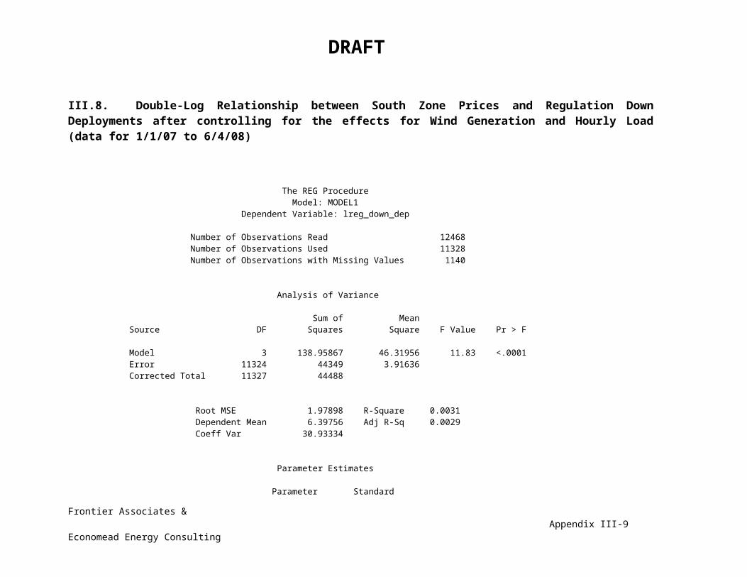
DRAFT

DateTime

(Interval Begin)

MCPE MW

1 if greater

than $1,000

True if consecutive

Number of Consecutive

Intervals

Price w/ DR Savings

4/25/2008 9:15 $2,316.68 0 1 TRUE 3 $347.50 $04/25/2008 9:30 $2,320.68 0 1 TRUE 4 $348.10 $05/19/2008 16:45 $2,250.00 412 1 FALSE 1 $337.50 $213,8635/19/2008 17:00 $2,250.00 417 1 TRUE 2 $337.50 $216,2535/19/2008 17:45 $2,250.00 414 1 TRUE 1 $337.50 $214,8195/20/2008 8:45 $1,307.97 871 1 FALSE 1 $196.20 $251,8995/20/2008 9:00 $2,069.02 1,089 1 TRUE 2 $310.35 $494,3155/20/2008 10:00 $2,084.28 1,056 1 TRUE 1 $312.64 $483,3445/20/2008 10:15 $2,086.68 1,060 1 TRUE 2 $313.00 $485,6755/28/2008 14:30 $2,250.00 1,048 1 FALSE 1 $337.50 $517,950

7/9/2008 22:00 $2,200.00 865 1 FALSE 1 $330.00 $420,8887/13/2008 13:45 $1,992.09 877 1 FALSE 1 $298.81 $386,1927/21/2008 22:00 $1,999.00 879 1 FALSE 1 $299.85 $388,381

8/7/2008 13:30 $1,999.00 1,034 1 FALSE 1 $299.85 $454,2238/7/2008 14:15 $1,999.00 897 1 TRUE 1 $299.85 $396,0278/7/2008 14:30 $1,999.00 932 1 TRUE 2 $299.85 $410,8948/7/2008 14:45 $1,999.00 969 1 TRUE 3 $299.85 $426,6128/7/2008 15:30 $1,999.00 869 1 TRUE 1 $299.85 $384,1338/7/2008 15:45 $1,999.00 987 1 TRUE 2 $299.85 $434,2588/7/2008 16:00 $1,999.00 756 1 TRUE 3 $299.85 $336,1328/7/2008 16:15 $1,999.00 754 1 TRUE 4 $299.85 $335,2828/7/2008 16:30 $1,999.00 754 1 TRUE 5 $299.85 $335,2828/7/2008 16:45 $1,999.00 754 1 TRUE 6 $299.85 $335,2828/7/2008 17:00 $1,999.00 927 1 TRUE 7 $299.85 $408,7718/7/2008 17:15 $1,999.00 903 1 TRUE 8 $299.85 $398,5768/7/2008 17:30 $1,999.00 893 1 TRUE 9 $299.85 $394,328

Frontier Associates &Appendix V-17

Economead Energy Consulting

DRAFT

DateTime

(Interval Begin)

MCPE MW

1 if greater

than $1,000

True if consecutive

Number of Consecutive

Intervals

Price w/ DR Savings

8/7/2008 18:00 $1,999.00 676 1 TRUE 1 $299.85 $302,1498/21/2008 15:45 $1,999.00 611 1 FALSE 1 $299.85 $274,5388/22/2008 13:45 $1,999.00 1,053 1 FALSE 1 $299.85 $462,2948/22/2008 14:30 $1,999.00 803 1 TRUE 1 $299.85 $356,097

10/13/2008 14:00 $1,999.00 1,222 1 FALSE 1 $299.85 $534,08310/13/2008 14:15 $1,999.00 1,222 1 TRUE 2 $299.85 $534,08310/13/2008 14:30 $1,999.00 1,222 1 TRUE 3 $299.85 $534,08310/13/2008 15:00 $1,999.00 354 1 TRUE 1 $299.85 $165,36710/13/2008 15:30 $1,999.00 793 1 TRUE 1 $299.85 $351,84910/13/2008 16:15 $1,999.00 793 1 TRUE 1 $299.85 $351,84910/13/2008 16:30 $1,999.00 793 1 TRUE 2 $299.85 $351,84910/13/2008 16:45 $1,999.00 793 1 TRUE 3 $299.85 $351,84910/13/2008 17:00 $1,999.00 793 1 TRUE 4 $299.85 $351,849

11/1/2008 10:30 $1,934.80 340 1 FALSE 1 $290.22 $154,30011/1/2008 10:45 $1,934.80 489 1 TRUE 2 $290.22 $215,56111/1/2008 11:00 $1,930.76 406 1 TRUE 3 $289.61 $181,05711/1/2008 12:00 $1,921.07 200 1 TRUE 1 $288.16 $96,05311/1/2008 12:15 $1,922.47 445 1 TRUE 2 $288.37 $196,212

3/1/2009 19:00 $2,130.24 676 1 FALSE 1 $319.54 $321,9863/1/2009 19:15 $2,135.08 818 1 TRUE 2 $320.26 $387,1433/1/2009 19:30 $2,143.26 1,213 1 TRUE 3 $321.49 $568,526

3/11/2009 17:30 $2,146.98 751 1 FALSE 1 $322.05 $358,7333/11/2009 17:45 $2,133.32 681 1 TRUE 2 $320.00 $324,7183/11/2009 20:00 $2,167.82 861 1 TRUE 1 $325.17 $412,8883/11/2009 20:15 $2,146.98 746 1 TRUE 2 $322.05 $356,4523/11/2009 23:15 $1,936.56 30 1 FALSE 1 $290.48 $14,524

Frontier Associates &Appendix V-18

Economead Energy Consulting

DRAFT

DateTime

(Interval Begin)

MCPE MW

1 if greater

than $1,000

True if consecutive

Number of Consecutive

Intervals

Price w/ DR Savings

3/12/2009 0:00 $1,940.90 0 1 TRUE 1 $291.13 $03/12/2009 0:15 $1,942.49 82 1 TRUE 2 $291.37 $39,8213/12/2009 0:30 $1,941.22 0 1 TRUE 3 $291.18 $0

Frontier Associates &Appendix V-19

Economead Energy Consulting

DRAFT

Appendix VI: Possible Increase in the Cost of Regulation Down due to Demand-Side Response to Prices

The annual cost imposed by regulation obligations was assessed by calculating the Regulation Down deployments that could potentially be attributable to “price chasing,” and then calculating the regulation down obligations associated with these deployments. These calculations used a linear equation that expresses the relationship of regulation down deployments and regulation down obligations, controlling for wind generation. Price chasing is assumed to be represented by regulation down deployments that have a linear relationship with price spikes above $300, controlling for the effects of wind generation.

Y (Regulation Down Deployments) = a + b * (north zone price spike > $300/MWh) + c * (wind generation)Y (Regulation Down Deployments) = a + b * (south zone price spike > $300/MWh) + c * (wind generation)Y (Regulation Down Deployments) = a + b * (Houston zone price spike > $300/MWh) + c * (wind generation)

Controlling for wind generation, according to the regression analyses in Appendices III.4-III.6:

Y (Regulation Down Deployments) = a + 195 * (north zone price spike) + c * (wind generation)Y (Regulation Down Deployments) = a + 345 * (south zone price spike) + c * (wind generation)Y (Regulation Down Deployments) = a + 435 * (Houston zone price spike) + c * (wind generation)

Using the count of price spikes for the year 2009 located Table 1 in the White Paper, the number of Regulation Down deployments for each region in 2009 can be counted.

Y (North Zone Regulation Down Deployments in 2009) = 195 * 21 = 4,095 MWh/yr 341 MWh/monthY (South Zone Regulation Down Deployments in 2009) = 345 * 3 = 1,035 MWh/yr 86 MWh/monthY (Houston Zone Regulation Down Deployments in 2009) = 435 * 11 = 4,785 MWh/yr 399 MWh/month

According to the regression analysis in Appendix IV:

Y (Regulation Down Obligations) = a + 0.0063 * (Regulation Down Deployments) + c * (wind generation)

Y (North Zone Regulation Down Obligations) = a + (0.0063) * (341 MWh/month) = 2.1 MW/month = 25.8 MW/yearY (South Zone Regulation Down Obligations) = a + (0.0063) * (86 MWh/month) = 0.5 MW/month = 6.5 MW/yearY (Houston Zone Regulation Down Obligations) = a + (0.0063) * (399 MWh/month) = 2.5 MW/month = 30.1 MW/year

North Zone 25.8 MW/year * $12/MW [cost] * 8760 [number of hours in a year] = $ 2,711,938/yearSouth Zone 6.5 MW/year * 12 * 8760 = $ 685,435/year

Frontier Associates & Appendix VI-1Economead Energy Consulting

DRAFT

Houston Zone 30.1 MW/year * 12 * 8760 = $ 3,168,895/year

Average cost of Regulation Down Obligations resulting from Regulation Down Deployments related to price spikes over $300 $ 2,188,756/year

Because the regression analysis in Appendix IV represents the entire system, rather than the zones, the estimated costs of Regulation Down obligations that have a linear relationship with Regulation Down deployments related to price spikes are averaged together. These costs average to $2,188,756 per year.

In 2009, the total savings from 500 MW of demand response was $12,535,746. The ability to respond to prices saves much more than any possible increase in the cost of Regulation Down that could be attributed to price chasing. The loss of pricing transparency may make price chasing impossible, but the loss of savings due to demand response is far more costly.

Frontier Associates & Appendix VI-2Economead Energy Consulting