data transformation by calculation

Data Transformation by Calculation

J.N. Oliveira

Dept. Informatica,Universidade do Minho

Braga, Portugal

GTTSE’072–7 July 2007

Braga

First lecture

Schedule: Monday July 2nd, 5pm-6pm

Learning outcomes:

• Identifying the problem

• Finding a strategy to face it

Motivation

• Data play an important role in our lifes (eg. medical records,bank details, CVs, ... )

• Information system quality is highly dependent uponconsistency and reliability of data

• Data are everywhere in computing — statically (eg. machinestates, databases) and dynamically (eg. messages, APIs,forms, etc)

• Data are what is left from the past (cf. historical archives)

However...

Motivation

• Data keep changing format

• No two people think data in the same way

• Data modeling is technology sensitive

• Impedance mismatch among data models

• Need for data migration software

• Data always put at risk — loss or damage

Motivation

Quoting Lammel and Meijer (GTTSE’05):

• “Whatever programming paradigm for data processing wechoose, data has the tendency to live on the other side or toeventually end up there. (...)

• This myriad of inter- and intra-paradigm data models calls fora good understanding of techniques for mappings betweendata models, actual data, and operations on data. (...)

• Given the fact that IT industry is fighting with variousimpedance mismatches and data-model evolutionproblems for decades, it seems to be safe to start a researchcareer that specifically addresses these problems”.

Our strategy in this tutorial:

Don’t invent data mappings any more: calculate them!

Interacting with machines

Problems can arise anywhere at any time: even using a pocketcalculator

digits

keyin

��binary

display

DD

digits need to reach the machine binary so that it... calculates!

digits digits

keyin

��binary

display

DD

binary√

gg

Likely faults

• digit displayed not always the one whose key was pressed(confusion)

• nothing at all displayed (loss)

• required operation yields wrong output (miscalculation)

What about “inside the machine”?

• HCI is just a special case of subcontracting (a service)

• Subcontracting spreads over mutiple layers, differenttechnologies

• Uncountable number of data mappings at work intransactions and layer inter-communication.

Weaving data through I-M-D architecture

Layered-architectures rely on sub-contracting:

@@R

@@R

@@R

��

��

��

DI M

rep′

rep

ret ′

ret

Legend:

I — interfaceM — middlewareD — datawarerep — representret — retrieve

The same in different geometry

Separation principles (eg. Seheim model, client-server, etc) entailpermanent data conversion across disparate technology layers:

onmlhijkI

rep,,wvutpqrsM

retr

kk

rep′

,,wvutpqrsD

retr ′ll

Running example — genealogy website (I)

At GUI level, clients wish to see and browse their family trees:

Margaret, b. 1923 Luigi, b. 1920

Mary, b. 1956 Joseph, b. 1955

SSSSSSmmmmmm

Peter, b. 1991

SSSSSSkkkkkk

(1)

Running example — genealogy website (M)

Treesbecome“moreconcrete” asthey go downthe layers ofsoftwarearchitecture;

• Margaret

1923

NIL

NIL

Mary

1956

NIL

NIL

Joseph

1955

•

•

Peter

1991

•

•

Luigi

1920

NIL

NIL

They convertto pointerstructures(eg. inC++/C#)stored indynamicheaps oncereachingmiddleware.

Running example — genealogy website (D)

Finally channeled to dataware, heap structures are buried intodatabase files as persistent data records:

ID Name Birth

1 Joseph 1955

2 Luigi 1920

3 Margaret 1923

4 Mary 1956

5 Peter 1991

ID Ancestor ID

5 Father 1

5 Mother 4

1 Father 2

1 Mother 3

Too many paradigms

Data modeling notations, eg. Entity-Relationship (ER) diagrams

Individual

ID

Name Birth

Parent

0:nof

0:2is

Too many paradigms

UML class diagrams

Individual

ID: StringName: StringBirth: Date

0..2

Parent

Too many paradigms

XML (version 1)



<!ELEMENT tree (node+)>

<!ELEMENT node (name, birth, mother?, father?)>

<!ELEMENT name (#PCDATA)>

<!ELEMENT birth (#PCDATA)>

<!ELEMENT mother EMPTY>

<!ELEMENT father EMPTY>

<!ATTLIST tree

ident ID #REQUIRED>

<!ATTLIST mother

refid IDREF #REQUIRED>

<!ATTLIST father

refid IDREF #REQUIRED>

Too many paradigms

XML (version 2)



<!ELEMENT tree (name, birth, tree?, tree?)>

<!ELEMENT name (#PCDATA)>

<!ELEMENT birth (#PCDATA)>

Too many (programming) paradigms

Plain SQL

CREATE TABLE INDIVIDUAL (

ID NUMBER (10) NOT NULL,

Name VARCHAR (80) NOT NULL,

Birth NUMBER (8) NOT NULL,

CONSTRAINT INDIVIDUAL_pk PRIMARY KEY(ID)

);

CREATE TABLE ANCESTORS (

ID VARCHAR (8) NOT NULL,

Ancestor VARCHAR (8) NOT NULL,

PID NUMBER (10) NOT NULL,

CONSTRAINT ANCESTORS_pk PRIMARY KEY (ID,Ancestor)

);

Too many (programming) paradigms

C/C++ etc

typedef struct Gen {

char *name /* name is a string */

int birth /* birth year is a number */

struct Gen *mother; /* genealogy of mother (if known) */

struct Gen *father; /* genealogy of father (if known) */

} ;

Haskell etc

data PTree = Node {

name :: [ Char ],

birth :: Int ,

mother :: Maybe PTree,

father :: Maybe PTree

}

Questions

• Are all these data models “equivalent”?

• If so, in what sense?

• If not, how can they be ranked in terms of “quality”?

• How can we tell apart the essence of a data model from itstechnology wrapping?

“The question”

Is there a notation unifying allthe above?

Keep it simple

Let us writec R a

to mean that

datum c (eg. byte) represents datum a (eg. digit)

and let the converse facta R◦ c

mean

a is the datum represented by c

(passive voice).

No confusion, please

Definite article “the” instead of “a” in sentence

a is the datum represented by c

already a symptom of the no confusion principle: we want c torepresent only one datum of interest.

So R should be injective:

〈∀ c , a, a′ :: c R a ∧ c R a′ ⇒ a = a′〉 (2)

No data loss, please

No loss principle: no data are lost in the representation process,

〈∀ a :: 〈∃ c :: c R a〉〉 (3)

ie. every datum a is representable — R is totally defined. In adiagram:

A

R

&&C

R◦

ff (4)

for R injective and totally defined

Freeing the retrieve relation

Useful (in general) to give some freedom to the retrieve relation,say F , provided that it connects with the chosen representation:

〈∀ a, c :: c R a ⇒ a F c〉 (5)

(=“if c represents a then a can be retrieved from c).

In a diagram:

A

R

''≤ C

F

gg (6)

(Meaning of ≤ to be explained soon.)

Mapping scenarios

Diagram

A

R

''≤ C

F

gg

already captures some of the ingredients of Lammel and Meijer’smapping scenarios:

• the type-level mapping of a source data model (A) to a targetdata model (C );

• two maps — “map forward” (R) and “map backward” (F )— between source / target data;

• the transcription level mapping of source operations intotarget operations — see next slide

Transcription level

Source (eg. CRUD) operations mapped to target operations —put two ≤-diagrams together:

A

R

''

O

��

≤ C

F

gg

P

��B

R′

''≤ D

F ′

gg

(7)

The (safe) transcription of O into P can be formally stated byensuring that the picture is a commutative diagram. (Detailssoon.)

Chaining

In general, it will make sense to chain two or more mappingscenarios, eg. between interface (I ) and middleware (M), andbetween middleware and dataware (D):

I

R

''≤ M

F

ff

R′

''≤ D

F ′

gg

However, how can we be sure that mapping scenarios composewith each other?

Data refinement

• All questions so far are addressed in the well studied disciplineof data refinement

• However, data refinement not “sexy enough” — too complex,too many symbols:

Can’t we do better?

Interlude

Problem-solving strategy

Recall the universal problem solving strategy which one is taught atschool:

• understand your problem

• build a mathematical model of it

• reason in such a model

• upgrade your model, if necessary

• calculate a final solution and implement it.

School maths example

The problem

My three children were born at a 3 year interval rate. Altogether,they are as old as me. I am 48. How old are they?

The model

x + (x + 3) + (x + 6) = 48

The calculation

3x + 9 = 48

≡ { “al-djabr” rule }

3x = 48 − 9

≡ { “al-hatt” rule }

x = 16 − 3

School maths example

The solution

x = 13x + 3 = 16x + 6 = 19

Questions....

• “al-djabr” rule ?

• “al-hatt” rule ?

Have a look at Pedro Nunes (1502-1578) Libro de Algebra enArithmetica y Geometria (dated 1567) . . .

Libro de Algebra en Arithmetica y Geometria (1567)

(...) the inventor of this

art was a Moorish

mathematician, whose

name was Gebre, & in

some libraries there is a

small arabic treaty which

contains chapters that we

use

(fol. a ij r)

Reference to On the calculus of al-gabr and al-muqabala by Abu

Al-Huwarizmı, a famous 9c Persian mathematician.

Calculus of al-gabr, al-hatt and al-muqabala

al-djabr

x − z ≤ y ≡ x ≤ y + z

al-hatt

x ∗ z ≤ y ≡ x ≤ y ∗ z−1(z > 0)

al-muqabala

Ex: 4x2 − 2x2 = 2x + 6 − 3 ≡ 2x2 = 2x + 3

“Algebra (...) is thing causing admiration”

(...) Principalmente que vemos algumas vezes, no poder vngran Mathematico resoluer vna question por mediosGeometricos, y resolverla por Algebra, siendo la misma Algebrasacada de la Geometria, q es cosa de admiracio.

ie.

(...) Mainly because we see often a great Mathematicianunable to resolve a question by Geometrical means, andsolve it by Algebra, being that same Algebra taken fromGeometry, which is thing causing admiration.

[ in Nunes’ Libro de Algebra, fols. 270–270v. ]

Letting “the symbols do the work” in the 16c

Deduction first

Y tambien porque quien obra por Algebra va entendiendo larazon de la obra que haze, hasta la yqualacion ser acabada.(...) De suerte que, quien obra por Algebra, va haziendodiscursos demonstrativos.

ie.

And also because one performing by Algebra isunderstanding the reason of the work one does, until theequality is finished. (...) So much so that, who works byAlgebra is doing a demonstrative discourse.

[ fol. 269r-269v ]

Verdict

(...) De manera, quequien sabe por Algebra,

sabe scientificamente.

(...) in this way, who knows by Algebraknows scientifically)

Trend for notation economy

Well-known throughout the history of maths — a kind of “naturallanguage implosion” — particularly visible in the syncopatedphase (16c), eg.

.40.p.2.ce. son yguales a .20.co

(P. Nunes, Coimbra, 1567) for nowadays 40 + 2x2 = 20x , or

B 3 in A quad - D plano in A + A cubo æquatur Z solido

(F. Viete, Paris, 1591) for nowadays 3BA2 − DA + A3 = Z

Later on (18c, 19c, . . . )

More demanding problems to be modelled/solved, eg. electricalcircuits:

From a simple law . . .

V = R × I by Georg Ohm (1789-1854) . . .

. . . to non-linear RC-circuitsv(t) = Ri(t) + 1

C

∫ t

0 i(τ)dτv(t) = V0(u(t − a) − u(t − b)) (b > a)

Calculate i(t)

The following i(t) can be observed on an oscilloscope:

Can you explain it?

Is 16c maths still enough for the required calculations?

No. Need for the differential/integral calculus.

But there is more:

For the underlying maths to scale up

Need for an integral transform, eg. the Laplace transform.

Laplace transform

t-space s-space

Given problem

y ′′ + 4y ′ + 3y = 0y(0) = 3y ′(0) = 1

//

Subsidiary equation

s2 + 4sY + 3Y = 3s + 13

��Solution of given problem

y(t) = −2e−3t + 5e−t

Solution of subs. equation

Y = −2s+3 + 5

s+1

oo

Laplace-transformed RC-circuit model

L(t-space RC model) is

RI (s) +I (s)

sC=

V0

s(e−as − e−bs)

whose algebraic solution for I (s) is

I (s) =V0R

s + 1RC

(e−as − e−bs)

Now, the converse transformation:

L−1(V0R

s + 1RC

) =V0

Re−

tRC

Analytical solution

After some algebraic manipulation we will obtain an analyticalanswer . . .

i(t) =

0 if t < a

(V0e−

aRC

R)e−

tRC if a < t < b

(V0e−

aRC

R− V0e

−b

RC

R)e−

tRC if t > b

Question

All we have seen applies to physics, mechanical eng., civil eng.,electrical and electronic eng.

What about us? (software engineers)

Need for a transform

Integration? Quantification?

(L f )s =∫ ∞0 e−st f (t)dt

f (t) L(f )

1 1s

t 1s2

tn n!sn+1

eat 1s−a

etc

A parallel:

〈

∫

x : 0 ≤ x ≤ 10 : x2 − x〉

〈∀ x : 0 ≤ x ≤ 10 : x2 ≥ x〉

An “s-space analog” for logical quantification

The pointfree (PF) transform

φ PF φ

〈∃ a :: b R a ∧ a S c〉 b(R · S)c〈∀ a, b : : b R a ⇒ b S a〉 R ⊆ S

〈∀ a :: a R a〉 id ⊆ R〈∀ x : : x R b ⇒ x S a〉 b(R \ S)a〈∀ c : : b R c ⇒ a S c〉 a(S / R)b

b R a ∧ c S a (b, c)〈R ,S〉ab R a ∧ d S c (b, d)(R × S)(a, c)b R a ∧ b S a b (R ∩ S) ab R a ∨ b S a b (R ∪ S) a(f b) R (g a) b(f ◦ · R · g)a

True b ⊤ aFalse b ⊥ a

What are R , S , id ?

End of interlude

A transform for logic and set-theory

An old idea

PF (sets, predicates) = binary relations

Calculus of binary relations

• 1860 - introduced by De Morgan, embryonic

• 1941 - Tarski’s school, cf. A Formalization of Set Theorywithout Variables

• 1980’s - coreflexive models of sets (Freyd and Scedrov,Eindhoven school)

Unifying approach

Everything is a (binary) relation

Binary Relations

Arrow notation

Arrow AR // B denotes a binary relation to B (target) from A

(source).

Identity of composition

id such that R · id = id · R = R

ConverseConverse of R — R◦ such that a(R◦)b iff b R a.

Ordering

“R ⊆ S — the “R is at most S” — the obvious R ⊆ S ordering.

Binary relation taxonomy

The whole picture:relation

injective entire simple surjective

representation function abstraction

injection surjection

bijection

where

Reflexive (⊇ id) Coreflexive (⊆ id)

ker R entire R injective R

img R surjective R simple R

ker R = R◦ · Rimg R = R · R◦

Second lecture

Schedule: Tuesday July 3rd, 11h30am-12h30m

Learning outcomes:

• PF-transform essentials

• PF-transform at work: describing data models and dataimpedance mismatch

Functions in one slide

• A function f is a relation such that b f a ≡ b = f a and

Pointwise Pointfree“Left” Uniqueness

b f a ∧ b′ f a ⇒ b = b′ img f ⊆ id (f is simple)Leibniz principle

a = a′ ⇒ f a = f a′ id ⊆ ker f (f is entire)

• Back to useful “al-djabr” rules:

f · R ⊆ S ≡ R ⊆ f ◦ · S

R · f ◦ ⊆ S ≡ R ⊆ S · f

• Equality:

f ⊆ g ≡ f = g ≡ f ⊇ g

Simple relations

Simple relations are everywhere in computing:

• As computations: partial functions are simple relations

• As data: (finite) simple relations model functionaldependencies, object identity, etc

• We will draw harpoon arrows B ARo or A

R /B toindicate that R is simple.

We shall be using (simple) relations to model both algorithms anddata.

Simple relations in one slide

“Al-djabr” rules for simple M:

M · R ⊆ T ≡ (δM) · R ⊆ M◦ · T (8)

R · M◦ ⊆ T ≡ R · δM ⊆ T · M (9)

where

δ R = ker R ∩ id

the domain of R is the coreflexive part of ker R .

Dually, we define the range of R as

ρR = img R ∩ id

Predicates PF-transformed

• Binary predicates :

R = [[b]] ≡ (y R x ≡ b(y , x))

• Unary predicates become fragments of id (coreflexives) :

R = [[p]] ≡ (y R x ≡ (p x) ∧ x = y)

eg. (in the natural numbers)

[[1 ≤ x ≤ 4]] =

Boolean algebra of coreflexives

[[p ∧ q]] = [[p]] · [[q]] (10)

[[p ∨ q]] = [[p]] ∪ [[q]] (11)

[[¬p]] = id − [[p]] (12)

[[false]] = ⊥ (13)

[[true]] = id (14)

Note the very useful fact that conjunction of coreflexives iscomposition

Simple relation expressive power

• Comprehension notation borrowed from VDM to denote a(finite) simple relation S at pointwise level:

{a 7→ S a | a ∈ dom S}

where dom S is the set-theoretic version of δ S .

• Useful PF patterns:

• projection — f · S · g◦ (g injective):

{g a 7→ f (S a) | a ∈ dom S}

• selection — Ψ · S · Φ (Ψ,Φ coreflexives):

{a 7→ S a | a ∈ dom S ∧ φ a ∧ ψ(S a)}

All (data structures) in one (PF notation)

ProductsDatabase records — eg. 5 Peter 1991 — C/C++structs etc are products:

A A × Bπ1oo π2 // B

C

R

ffMMMMMMMMMMMMM

〈R,S〉OO

S

88qqqqqqqqqqqqq

(15)

where

ψ PF ψ

a R c ∧ b S c (a, b)〈R ,S〉cb R a ∧ d S c (b, d)(R × S)(a, c)

(16)

Clearly: R × S = 〈R · π1,S · π2〉

Sums

Example (Haskell):

data X = Boo Bool | Err String

PF-transforms to

Booli1 //

Boo))SSSSSSSSSSSSSSSSSS Bool + String

[Boo ,Err ]

��

Stringi2oo

Erruukkkkkkkkkkkkkkkkkk

X

(17)

where

[R ,S ] = (R · i◦1 ) ∪ (S · i◦2 ) cf. Ai1 //

R&&MMMMMMMMMMMMM A + B

[R ,S]

��

Bi2oo

Sxxqqqqqqqqqqqqq

CDually: R + S = [i1 · R , i2 · S ]

Polynomial types and grammars

• With sums and products one can build polynomials,“pointers” included:

Maybe Adef= A + 1 (18)

(where 1 is the singleton type inhabited by Nil):

• Grammars:

Bnf notation Polynomial notation

α | β 7→ α+ βαβ 7→ α× βǫ 7→ 1a 7→ 1

(19)

Grammars and inductive data models

For instance,

X → ǫ | a A X

(where X ,A are non-terminals and a is terminal) leads equation

X = 1 + A × X (20)

cf.

typedef struct x {

A data;

struct x *next;

} Node;

typedef Node *X;

since 1 + A × X is an instance of the “pointer to struct” pattern.

PF-transformed PTreedata PTree = Node { name :: [ Char ], birth ::

Int , mother :: Maybe PTree, father :: Maybe

PTree }

becomes

PTree ∼= Ind × (PTree + 1) × (PTree + 1) (21)

where Ind = Name × Birth packages the information relative tothe name and birth year, ie.

PTree ∼= G(Ind ,PTree) (22)

where G captures the particular pattern of recursion chosen tomodel family trees

G(X ,Y )def= X × (Y + 1) × (Y + 1)

( X refers to the parametric information and Y to the inductivepart.)

Entity-Relationship diagrams

PF-transform of

BookISBNTitleAuthor[0-5]Publisherid: ISBN

ReservedDate

BorrowerPIDNameAddressPhoneid: PID

0:N 0:N

is

Dbdef= Books × Borrowers × Reserved

Booksdef= ISBN ⇀ Title × (5 ⇀ Author) × Publisher

Borrowersdef= PID ⇀ Name × Address × Phone

Reserveddef= ISBN × PID ⇀ Date

Business rules

Example

“(...) Only existing books can be borrowed by known borrowers”

Pointwise

φ(M,N,R)def=

〈∀ i , p, d :: d R (i , p) ⇒ 〈∃ x :: x M i〉 ∧ 〈∃ y :: y M p〉〉

where i , p, d range over ISBN,PID and Date, respectively,

PF-transformWe first order relations by how defined they are,

R � S ≡ δ R ⊆ δ S

Then...

Business rulesRule

φ(M,N,R)def= R � M · π1 ∧ R � N · π2

cf. diagram

ISBN

M

�

ISBN × PID

R

�

π1oo π2 // PID

N

�Title × (5 ⇀Author) ×Publisher

DateName×Address×Phone

whose geometrical similarity with the original is striking, recall:

BookISBNTitleAuthor[0-5]Publisherid: ISBN

ReservedDate

BorrowerPIDNameAddressPhoneid: PID

0:N 0:N

Data impedance mismatch expressed in the PF-style

A

R

''≤ B

F

gg where

• ker R = id (representation) and imgF = id (abstraction)• connection between (R ,F )

〈∀ a, b :: b R a ⇒ a F b〉

shrinks to

R◦ ⊆ F (23)

(=R◦ is the least retrieve relation associated with R)equivalent to

R ⊆ F ◦ (24)

(= F ◦ largest representation one can connect to retrieverelation F ).

≤ is a preorder

• ≤ is reflexive: Between a datatype and itself

A

id

''≤ A

id

gg

there is no impedance at all

• ≤ is transitive:

A

R

''≤ B

F

gg ∧ B

S

''≤ C

G

gg ⇒ A

S·R''

≤ C

F ·G

gg

that is, data impedances compose.

One slide long calculations

(F · G ,S · R) are connected:

S · R ⊆ (F · G )◦

≡ { converses: (R · S)◦ = S◦ · R◦ }

S · R ⊆ G ◦ · F ◦

⇐ { monotonicity }

S ⊆ G ◦ ∧ R ⊆ F ◦

≡ { since S ,G and R ,F are assumed connected }

True

Right-invertibility

That ≤-rules entail right-invertibility

F · R = id (25)

is again a one slide long calculation:

F · R = id

≡ { equality of relations }

F · R ⊆ id ∧ id ⊆ F · R

≡ { imgF = id and kerR = id }

F · R ⊆ F · F ◦ ∧ R◦ · R ⊆ F · R

≡ { converses }

F · R ⊆ F · F ◦ ∧ R◦ · R ⊆ R◦ · F ◦

⇐ { (F ·) and (R◦·) are monotone (cf. GCs) }

R ⊆ F ◦ ∧ R ⊆ F ◦

Functions only

Right-invertibility happens to be equivalent to connectivitywherever both abstraction and representation are functions, sayf , r :

A

r

''≤ C

f

gg ≡ f · r = id (26)

That f · r = id equivales r ⊆ f ◦ and entails f surjective and rinjective is again a short calculation:

f · r = id

≡ { equality of functions }

f · r ⊆ id

≡ { “al-djabr” (shunting) }

r ⊆ f ◦

Functions only

r ⊆ f ◦

⇒ { composition is monotonic }

f · r ⊆ f · f ◦ ∧ r◦ · r ⊆ r◦ · f ◦

≡ { f · r = id ; converses }

id ⊆ f · f ◦ ∧ r◦ · r ⊆ id

≡ { definitions }

f surjective ∧ r injective

Equivalence: ⇒ (above) + ⇐ (which of holds in general)

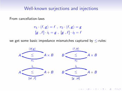
Well-known surjections and injections

From cancellation-laws

π1 · 〈f , g〉 = f , π2 · 〈f , g〉 = g

[g , f ] · i1 = g , [g , f ] · i2 = f

we get some basic impedance mismatches captured by ≤-rules:

A

〈id,g〉**

≤ A × B

π1

gg B

〈f ,id〉**

≤ A × B

π2

hh

A

i1**

≤ A + B

[id ,f ]

gg B

i2**

≤ A + B

[g ,id]

hh

Pointers and references

Pointers

A

i1))

≤ A + 1

[id ,F ]

gg

References (“references cheaper to move around than referents”)

G A

R++

≤ (IN ⇀ A) × G IN

Dref

jj (27)

cf. containers, shapes etc — details to be given later on.

Isomorphic data types

A quite special case of (r , f ) pair is one such that both

A

r

''≤ C

f

gg ∧ A

f

''≤ C

r

gg (28)

hold. This equivales

r ⊆ f ◦ ∧ f ⊆ r◦

≡ { converses ; equality of relations }

r◦ = f (29)

So r (a function) is the converse of another function f . Thismeans that both are bijections (isomorphisms) since

f is a bijection ≡ f ◦ is a function (30)

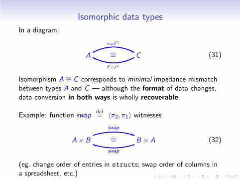
Isomorphic data types

In a diagram:

A

r=f ◦

''∼= C

f =r◦

gg (31)

Isomorphism A ∼= C corresponds to minimal impedance mismatchbetween types A and C — although the format of data changes,data conversion in both ways is wholly recoverable.

Example: function swapdef= 〈π2, π1〉 witnesses

A × B

swap

**∼= B × A

swap

jj (32)

(eg. change order of entries in structs; swap order of columns ina spreadsheet, etc.)

When the converse of a function is a function

swap◦

= { 〈R , S〉 = π◦

1 · R ∩ π◦

2 · S }

(π◦1 · π2 ∩ π◦2 · π1)

◦

= { converses }

π◦2 · π1 ∩ π◦1 · π2

= { back to splits }

swap

So swap is its own inverse and therefore a bijection.

Exercise 12, page 169

The calculation just above was too simple. To recognize the powerof rule “when the converse of a function is a function” prove theassociative property of sum,

A + (B + C )

r,,

∼= (A + B) + C

f =[id+i1 ,i2·i2]ll

(33)

by calculating the function r which is the converse of f .

[id + i1 , i2 · i2]◦

= { expand [R , S ] }

((id + i1) · i◦1 ∪ i2 · i2 · i

◦2 )◦

= { converses }

i1 · (id + i◦1 ) ∪ i2 · i◦2 · i◦2


i1 · (id + i◦1 ) ∪ i2 · i◦2 · i◦2 (from last slide)

= { expand R + S }

i1 · [i1 , i2 · i◦1 ] ∪ i2 · i

◦2 · i◦2

= { expand [R , S ] }

i1 · (i1 · i◦1 ∪ i2 · i

◦1 · i◦2 ) ∪ i2 · i

◦2 · i◦2

= { distribution ; associativity }

i1 · i1 · i◦1 ∪ (i1 · i2 · i

◦1 ∪ i2 · i

◦2 ) · i◦2

= { wrap up (function!) }

[i1 · i1 , [i1 · i2 , i2]]

= { spruce it }

[i1 · i1 , i2 + id ]


The following are known isomorphisms involving sums andproducts:

A × (B × C ) ∼= (A × B) × C (34)

A ∼= A × 1 (35)

A ∼= 1 × A (36)

A + B ∼= B + A (37)

C × (A + B) ∼= C × A + C × B (38)

Guess the relevant isomorphism pairs.

More elaborate isomorphisms

Let us introduce variables in isomorphism pair (r , f ):

r◦ = f

≡ { introduce variables }

〈∀ a, c :: c (r◦) a ≡ c f a〉

≡ { b(f ◦ · R · g)a ≡ (f b)R(g a) }

〈∀ a, c :: r c = a ≡ c = f a〉

You’ve seen this pattern already at school, recall eg.

〈∀ a, c :: b + c = a ≡ c = a − b〉 (39)

Let us see a few data transformations which share this pattern.

Transposes

Every relation can be safely converted into a the correspondingset-valued function:

〈∀ R , k :: k = ΛR ≡ R = ∈ · k〉 (40)

With more variables (omitting outer ∀):

k = ΛR ≡ 〈∀ b, a :: b R a ≡ b ∈ (k a)〉

Diagram:

(PB)A

(∈·)**

∼= A → B

Λ

jj

Transposes

Simple relations “are Maybe functions”:

k = tot S ≡ S = i◦1 · k

With more variables (omitting outer ∀):

k = tot S ≡ 〈∀ b, a :: b S a ≡ (i1b) = k a〉

Diagram:

(B + 1)A

untot=(i◦1 ·)**

∼= A ⇀ B

tot

kk

(Handles impedance mismatch between pointer data models andrelational models.)

Relational currying

Isomorphism

(C → A)B

( )◦

++∼= B × C → A

( )

kk(41)

and associated universal property,

k = R ≡ 〈∀ a, b, c :: a (k b) c ≡ a R (b, c)〉 (42)

express a kind of selection/projection mechanism: given some b0,R b0 selects the “sub-relation” of R of all pairs (a, c) related to b0.

Functional currying

Isomorphism (in case R := f )

(AC )B

( )◦

**∼= AB×C

( )

jj (43)

Associated universal property

k = f ≡ 〈∀ b, c :: (k b) c = f (b, c)〉 (44)

simpler because f is a function. (The usual notation for f iscurry f , and uncurry = curry◦.)

Third lecture

Schedule: Thursday July 5th, 11h30am-12h30m

Learning outcomes:

• PF-transform at work:• new ≤-rules from old• calculating implementations from abstract models• dealing with recursive data model impedance mismatch

• PF-transform in the lab: the 2LT package

• Topics for research

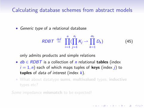
Calculating database schemes from abstract models

• Generic type of a relational database

RDBTdef=

n∏

i=1

(

ni∏

j=1

Kj ⇀

mi∏

k=1

Dk) (45)

only admits products and simple relations

• db ∈ RDBT is a collection of n relational tables (indexi = 1, n) each of which maps tuples of keys (index j) totuples of data of interest (index k).

• What about datatype sums, multivalued types, inductivetypes etc?

Some impedance mismatch to be expected!

Getting rid of sums

Diagram:

(B + C ) → A

[ , ]◦

,,∼= (B → A) × (C → A)

[ , ]

ll(46)

Universal property:

T = [R ,S ] ≡ T · i1 = R ∧ T · i2 = S (47)

Pragmatics: when applied from left to right, this rule helps inremoving sums from data models: relations with input sumsdecompose into pairs of relations

Getting rid of sums

What about sums at the output? Another sum-elimination rule isapplicable to such situations,

A → (B + C )

△+,,

∼= (A → B) × (A → C )

+⋊⋉

ll(48)

where

M+⋊⋉ N

def= i1 · M ∪ i2 · N (49)

△+ Mdef= 〈i◦1 · M, i◦2 · M〉 (50)

Getting rid of multivalued attributes

Recall that

Booksdef= ISBN ⇀ Title × (5 ⇀ Author) × Publisher

has a multivalued type (up to 5 authors). How do we remove(⇀)-nesting?

In the next slide we calculate a rule which gets rid of pattern

A ⇀ (D × (B ⇀ C ))

New ≤-rules from old

A ⇀ (D × (B ⇀ C ))

∼= { Maybe transpose }

(D × (B ⇀ C ) + 1)A

≤ { exercise 10 }

((D + 1) × (B ⇀ C ))A

∼= { splitting: (B × C )A ∼= BA × CA }

(D + 1)A × (B ⇀ C )A

∼= { Maybe transpose and relational (un)currying }

(A ⇀ D) × (A × B ⇀ C )

Getting rid of multivalued attributes

In summary:

A ⇀ (D × (B ⇀ C ))

△n

--≤ (A ⇀ D) × (A × B ⇀ C )

⋊⋉n

mm(51)

Illustration:

Books = ISBN ⇀ (Title × (5 ⇀ Author) × Publisher)

∼=1 { r1 = id ⇀ 〈〈π1, π3〉, π2〉 , f1 = id ⇀ 〈π1 · π1, π2, π2 · π1〉 }

ISBN ⇀ (Title × Publisher) × (5 ⇀ Author)

≤2 { r2 = △n , f2 = ⋊⋉n, cf. (??) }

(ISBN ⇀ Title × Publisher) × (ISBN × 5 ⇀ Author)

= Books2

Checking model transformations

Entity-Relationship PF-semantics makes it possible to checkmodel transformation rules available from the literature, eg.Rule 12.2 of J.-L. Hainaut (GTTSE’05) catalogue:

AA1A2A3[0:N]id: A1

⇔

A’A1A2id: A1

rA0:N

EA3K3A3id: K3

1:N

(This converts a 0 : N attribute into an entity.)

Starting point

A = A1 ⇀ A2 × PA3

Checking model transformations

A1 ⇀ A2 × PA3

≤1 { create references to A3 }

(K3 ⇀ A3) × (A1 ⇀ A2 × PK3)

∼=2 { PA ∼= A ⇀ 1 }

(K3 ⇀ A3) × (A1 ⇀ A2 × (K3 ⇀ 1))

≤3 { unnest (⇀) }

(K3 ⇀ A3) × ((A1 ⇀ A2) × (A1 × K3 ⇀ 1))

∼=4 { introduce ternary product }

(A1 ⇀ A2)︸︷︷︸

A′

× (P(A1 × K3))︸︷︷︸

rA

× (K3 ⇀ A3)︸︷︷︸

EA3

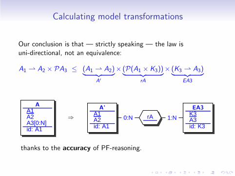
Calculating model transformations

Our conclusion is that — strictly speaking — the law isuni-directional, not an equivalence:

A1 ⇀ A2 × PA3 ≤ (A1 ⇀ A2)︸︷︷︸

A′

× (P(A1 × K3))︸︷︷︸

rA

× (K3 ⇀ A3)︸︷︷︸

EA3

AA1A2A3[0:N]id: A1

⇒

A’A1A2id: A1

rA0:N

EA3K3A3id: K3

1:N

thanks to the accuracy of PF-reasoning.

On the impedance of recursive data models

Recall that our starting model for family trees is recursive:

data PTree = Node {

name :: String ,

birth :: Int ,

mother :: Maybe PTree,

father :: Maybe PTree

}

that is (for Ind abbreviating name and birth)

PTree ∼= Ind × (PTree + 1) × (PTree + 1)︸︷︷︸

G PTree

In general

µG ∼= GµG

Getting rid of µ’s

µG

R --

≤(K ⇀ G K )︸︷︷︸

“heap”

×K

Unf

ii (52)

where K ia as a data type of “heap addresses” and K ⇀ G K adatatype of G-structured heaps.

Representations are “folds”

A typical representation R is the function r which builds the heapfor a tree by joining (separated) heaps for the subtrees, for instance

r (Node n b m f) = let x = fmap r m

y = fmap r f

in merge (n,b) x y

where merge performs separated union of heaps

merge a Nothing Nothing =

Heap ([ 1 |-> (a, Nothing, Nothing) ]) 1

merge a (Just x) (Just y) =

Heap ([ 1 |-> (a, Just k1, Just k2) ] ++ h1 ++ h2) 1

where (Heap h1 k1) = bmap id even_ x

(Heap h2 k2) = bmap id odd_ y

....

....

Data “heapification”

Source

t= Node {name = "Peter", birth = 1991,

mother = Just (Node {name = "Mary", birth = 1956,

mother = Nothing,

father = Just (Node {name = "Jules",

birth = 1917,

...... }}}

“heapifies” into:

r t = Heap [(1,(("Peter",1991),Just 2,Just 3)),

(2,(("Mary",1956),Nothing,Just 6)),

(6,(("Jules",1917),Nothing,Nothing)),

(3,(("Joseph",1955),Just 5,Just 7)),

(5,(("Margaret",1923),Nothing,Nothing)),

(7,(("Luigi",1920),Nothing,Nothing))]

1

Abstractions are “unfolds”

Abstraction is a (partial!) unfold:

f (Heap h k) = let Just (a,x,y) = lookup k h

in Node (fst a)(snd a)

(fmap (f . Heap h) x)

(fmap (f . Heap h) y)

(can be “totalized” via the Maybe transpose yielding a monadicunfold)

Thanks to the ≤-rule

f (r t) = t always holds.

Boiling recursion down to SQL

PTree∼=1 { r1 = out , f1 = in, for GK

def= Ind × (K + 1) × (K + 1) }

µG

≤2 { R2 = Unf ◦, F2 = Unf }

(K ⇀ Ind × (K + 1) × (K + 1)) × K

∼=3 { r3 = (id ⇀ flatr◦) × id , f3 = (id ⇀ flatr) × id }

(K ⇀ Ind × ((K + 1) × (K + 1))) × K

∼=4 { r4 = (id ⇀ id × p2p) × id , f4 = (id ⇀ id × p2p◦) × id }

(K ⇀ Ind × (K + 1)2) × K

∼=5 { r5 = (id ⇀ id × tot◦) × id , f5 = (id ⇀ id × tot) × id }

(K ⇀ Ind × (2 ⇀ K )) × K

≤6 { r6 = △n , f6 = ⋊⋉n }

Boiling recursion down to SQL

((K ⇀ Ind) × (K × 2 ⇀ K )) × K

∼=7 { r7 = flatl , f7 = flatl◦ }

(K ⇀ Ind) × (K × 2 ⇀ K ) × K

=8 { since Ind = Name × Birth }

(K ⇀ Name × Birth) × (K × 2 ⇀ K ) × K

In summary:

• Step 2 moves from the functional (inductive) to the pointer-basedrepresentation.

• Step 5 starts the move from pointer-based to relational-basedrepresentation: pointers “become” primary/foreign keys.

• Steps 7 and 8 deliver the final RDBT structure. (Third factor Kgives access to the root of the original tree.)

Last but not least

≤-calculus is structural: given parametric type G,

A

R

''≤ B

F

gg ⇒ G A

G R

((≤ G B

G F

hh

• Easy PF-proof (see notes)

• Also valid for n parameter types, eg.

A ≤ C ∧ B ≤ D ⇒ A + B ≤ C + D

Tools: 2LT (@ UMinho Haskell Libraries)

The 2LT engine is based on strategic term rewriting.

2LT demos: {XML,VDM} ↔ SQL

Demo 1:

• Bridging XML and SQL:• PTree example replayed by 2LT

Demo 2:

• Generating SQL from VDM data models:• Project: development of a repository of courses on formal

methods in Europe• Client: Formal Methods Europe (FME) association• Method: formal model in VDM++ lead to a prototype

webservice (using CSK VDMTools); database modelautomatically calculated by 2LT, including data migration.

Conclusions

Summary

• Data model impedance mismatch can be calculated

• PF-transform makes calculations agile and elegant

• e = m + c approach to software engineering

Topics in the notes not covered in the lectures

• Operation transcription (more technical but great fun)

• Concrete invariant calculation

Still a lot of work to do: see next slides

Research topic: Lenses relate to ≤-rules

Not only connectivity of

T × S putback

!!T

π◦

1 00

≤ S

get

ii

cf.

putback · π◦1 ⊆ get◦

≡ { “al-djabr” twice (functions) }

get · putback ⊆ π1

≡ { equality of functions }

get · putback = π1

≡ { add variables: acceptability }

get(putback(v , s)) = v

Lenses relate to ≤-rules

... but also connectivity of:

S

〈get,id〉**

≤ T × S

putback

gg

cf.

〈get, id〉 ⊆ put◦

≡ { “al-djabr” }

putback · 〈get, id〉 ⊆ id

≡ { add variables: stability }

putback(get s, s) = s

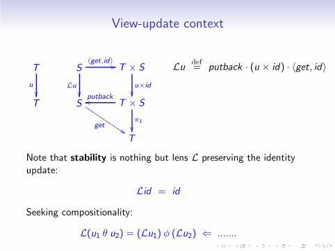
View-update context

T

u

��

S

Lu

��

〈get,id〉 // T × S

u×id

��T S

get$$JJJJJ

JJJJJJ T × Sputbackoo

π1

��T

Ludef= putback · (u × id) · 〈get, id〉

Note that stability is nothing but lens L preserving the identityupdate:

Lid = id

Seeking compositionality:

L(u1 θ u2) = (Lu1) φ (Lu2) ⇐ .......

Other research topics and applications

Heapification Law given can be generalized to mutually recursivedatatypes

Separation logic Law given has a clear connection toshared-mutable data representation and thus withseparation logic.

Concrete invariants ≤-rules should be able to take data typeinvariants into account

Mapping scenarios for the UML A calculational theory of UMLmapping scenarios could be developed from eg. KevinLano’s catalogue

2LT Tool can be of help in industrial applications (about70% of data-warehousing projects fail because offaulty data migrations!)

data transformation by calculation

Documents