department of aerospace engineeringcgpl.iisc.ernet.in/site/portals/0/publications/final...sdb report...
TRANSCRIPT

SDB Report 2006, CGPL, Dept of Aerospace Engineering, IISc, Bangalore Page No.1
Final Report on Strategic Development of Bio-Energy (SDB) Project
Technical report
Combustion, Gasification & Propulsion Laboratory (CGPL) Department of Aerospace Engineering
Indian Institute of Science Bangalore 560 012

SDB Report 2006, CGPL, Dept of Aerospace Engineering, IISc, Bangalore Page No.2
Contents Page Nos.
EXECUTIVE SUMMARY 3
PART I Preface 10
Chapter I The Gasification Process 11
Chapter II
Gasifiers with Biomass Briquettes and Low Grade Fuels for Power Generation for Industrial Application Introduction
17
Chapter III Biomass Gasification systems for High Grade Thermal Application in the Industrial Sector
46
Chapter IV Development of Power Package for Plastic Residues and Effluents from the Industrial and Urban Wastes
51
Chapter V Field Testing and Evaluations 58
PART II Preface 71
Chapter I Introduction and Literature Review 73
Chapter II Producer gas Properties 83
Chapter III The Experimental Work 85
Chapter IV Zero-Dimensional Model Formulation 116
Chapter V Laminar Burning Velocity Calculations 124
Chapter VI CFD Modelling 132
Chapter VII Predictions of Zero-D Model 151
Chapter VIII
Adaptation of Cummins Gas Engines for Use with Gasifiers for Power Generation
186
Chapter IX Development of Environmentally Clean Applications with Biomass Gasifiers for Power Generation
194
Chapter X Overview 204
Chapter XI Non-Edible Seed-Oils for Power Generation with Engines in Single or Dual Fuel Mode
207
PART III Preface 225
Chapter I
Package Development for Power Generation by Coconut Shell Based Agro-Residue Gasification with Generation of Activated Carbon
226
Chapter II Precipitated Silica from Rice Husk Ash IPSIT (Indian Institute of Science Precipitated Silica Technology)
240
Chapter III Biomass Preparation systems 244
Chapter IV Water Treatment for Gasification 259
SDB Report 2006, CGPL, Dept of Aerospace Engineering, IISc, Bangalore Page No.3
Executive Summary
This work is related to developing and establishing a gasifier technology to handle a range of bio-fuels in a single system. The establishment of the gasifier technology implies the development of the reactor, the cooling and cleaning system, and aspects of biomass processing at appropriate scales, drying the biomass, and a process for treating the effluents (of the cooling water) so that they can be recycled. It was important to understand and establish the operation with a reciprocating gas engine on producer gas by doing necessary basic research as such a research has not been performed adequately internationally. Also the aspects of generating value added products like activated carbon and precipitated silica were intended to be addressed to improve the plant economics. This is the reason for terming this project Strategic Development of Bio-energy. As will be seen in this report, all the aims of this project have been fulfilled. It is relevant to bring out that this project is a sequel to another on pulverizable fuels, called “POBIG” that was intended to deal with mostly agro-residues like rice husk, and sugarcane trash. Towards the end of this project POBIG in 1997, the central issues on the boundaries of performance were clear. The key idea of obliterating the origins of the fuel by pulverizing them was considered reasonable to start with. Several aspects and differences of cyclone type gasifiers from solid fuel gasifiers were recognized, particularly because open top downdraft re-burn gasifiers were being tested in the laboratory and operated in the field for reasonable times It was only using wood or wood like agro-residues – coconut shell or corncobs (those with high density and low ash content) . These differences are brought out as under.
a. The process of gasification in cyclone type systems needed control on the fuel and air
flow rates on a continuous basis. The response time of the system being of the order of seconds would result in changes in air-to-fuel ratio too quickly. This would result in the operation deviating from the set value to both richer and leaner sides leading to compositional variations. This in itself can be combated by an intermediate storage. But if it went richer, the tar generated could become more than acceptable. In the case of solid fuel gasifiers of downdraft open top re-burn type, the air-to-fuel ratio adjustment would be self-governed over the turn-down ratio.
b. A fundamental feature that was being researched during this period on liquid bio-fuels
from thermo-chemical conversion route in different laboratories across the world became known. To produce higher liquid fraction from the biomass, the biomass had to be heated at a very high heating rate (about 1000 C/s). This was possible only if the fuel was pulverized. Thus the route that was being adopted through cyclone gasification was good for generating liquid fuels. If we take that larger fraction of liquid are generated in the cyclone gasifiers, it would be necessary to provide sufficient residence time in the high temperature zones inside the reactor for cracking down the liquids to gases. This was intended due to other aspects of the design and it was considered that the residence time would be adequate (about a few seconds). It must also be remarked that significant cracking would be taking place. Even so the “hot tar” level observed was in the range of a 1000 ppm, a value that is several times compared to what would be obtained in a solid fuel system. It was inferred that the operation of cyclone gasifiers had to accept this limitation because of the approach – using pulverized fuels. Hence, one would need to conclude that cyclone gasifiers

SDB Report 2006, CGPL, Dept of Aerospace Engineering, IISc, Bangalore Page No.4
would not be able to produce engine quality gas unless there is more elaborate tar clean up system, something not required for a solid fuel gasification system.
c. One could imagine that because the processing of the fuel limits itself to drying and
pulverizing, there will be economic advantages in their use in this manner at least for thermal applications. Even if one were to overcome the fluctuations in the air-to-fuel ratio through a responsive control system, the fine particulate matter that would escape the cyclone gasifier would need to be captured to limit the emissions from any system that uses this approach.
It was in consideration of these facts that it was thought more appropriate to add one additional step to pre-processing. The briquetting process could be expected to densify the biomass about a 1000 kg/m3. There was an accompanying economic benefit – transportation would be made more economic since the material is densified. Thus a new thinking process that was wholesome was put together. Biomass drying, pulverizing and briquetting could be contemplated at various locations and the material transported to the power station. This would allow distributed operations and hence greater job opportunities and a more professional power plant operation that receives prepared good fuel. This implied that one had to investigate the IISc design of open downdraft re-burn system to determine the design aspects for accepting the agro-residue based briquettes. Agro-residues are characterized by significant inorganic content and the presence of problematic inorganic element, namely, potassium. The problem posed by potassium in classical combustion systems used by high pressure boilers (for power generation) is that potassium compounds, more particularly, potassium oxide related deposits in the sections of boiler tubing in a manner that even soot blowing is inadequate to dislodge the deposits. Hence the heat transfer process is affected over a relatively short period of time and the entire tubing has to be replaced. The alternate solution is to use the fuel in a gasification system, clean the gas and use in the combustion system (or even a reciprocating engine). This creates another problem. Potassium salts have the propensity to bring down the ash fusion temperature. Most agro-residues carry with them varying amounts of potassium depending on the amount of fertilizer applied during the agricultural operations. It is therefore important to determine the ash fusion temperature and more particularly, if the briquettes have the problem of ash fusion when used in the gasification system. In the case of closed top systems, the local temperatures that are generated at locations close to the air injection nozzles, exceed 1300 0C in most cases. Such a condition is sure to lead to ash fusion and this will prevent the gasifier operation from the moment ash fusion has occurred. In the case of IISc design, there is facility to share the air flow between the open top and the side air nozzles; it is possible to control the temperature distribution through the reactor because the flow velocities and the oxygen levels will get controlled. In the case of large reactors for large power levels, the IISc design has to use air injection at multiple locations along the reactor to ensure that air flow is distributed across the section as uniformly as possible. The presence of significant amount of ash demands a positive way to extracting it and it was thought that the approach of shaking the grate would be far from being adequate and no where near a positive way of extraction. To achieve this, a screw extraction technique was adopted. This was developed over several laboratory experiments and field experiences. The way the char would arrange itself inside the bottom section, the flow velocities through the bed and in the bottom section had to be limited to ensure little material carry over into the cyclone (the next element in the flow path). A vertical grate was introduced and its height

SDB Report 2006, CGPL, Dept of Aerospace Engineering, IISc, Bangalore Page No.5
was found critical to smooth operation. Subsequently, two short vertical grates were introduced. Early gas cleaning systems developed from small size systems had a sand bed filter. At large power levels and throughputs, the dead volume inside the system was large. This led to possibilities of explosion in unintended circumstances. To avoid large gas volumes, it was thought that the cleaning process must involve intense jet mixing processes in the fluid path. Impinging jet arrangements so familiar in liquid rocket engine design was adopted here. Not only was the momentum transfer to the gas substantive, the liquid break-up processes generated more intense mixing and better removal of particulate matter. There was always a final fabric filter that was expected to remove particulate matter in the size range of 10 microns to ensure that engine operations are smooth. This arrangement was found adequate for naturally aspirated engines whose tolerance to particulate matter was reasonable. In the case of turbo-supercharged engines this degree of clean up was found inadequate. It was found necessary to invent another technique – use of a chilled scrubber to exploit a different mechanism for particle removal – the condensation of water vapor on fine particulate matter at the low temperature offered a separate opportunity for removal of particulate matter. There is often a mistaken feeling among gasification community particularly the manufacturers had noted the success of chilled scrubber in IISc gasification system to adopt it in their own gasification systems without other considerations. Even if the issue of patent violation is set aside, it is to be understood that each system cleans up a fraction of the input. If the input is very large there will be a substantive amount in the downstream segment also. Hence simple adoption of chilled scrubber in the downstream section alone is not going to bring down the particulate matter to the levels that an IISc clean up system would do. Thus the gasifier finally developed resembled its WWII cousin no more. The bulky fuel carrier of the reactor was made cylindrical throughout. The throat was eliminated. Top was kept open. Staged air injection was adopted including air ingestion from the open top. The ash was extracted by a separate screw instead of grate. There was a vertical grate (or two depending on the size) instead of horizontal one. The cooling and cleaning system included specially designed scrubbers and an additional chilled scrubber. The final fabric filter was set to remove matter less than even 5 microns. All the developments, laboratory tests, field system evaluation and correction if any were all accomplished under this project. It is only befitting to state that without this major project, the developments at the laboratory would not have reached the field and got perfected as well as they have. The second important segment of the work is related to the engines. At the time the project was begun, there was no engine running on producer gas in the country. The only worthwhile literature was the work of the German company Imbert-Energietechnik GmbH & Co. that had put together power plants in East Africa, Guyana and Parguay. The largest of the plants of 3 x 465 kWe is supposed to be operated for reasonable time before the operations closed down. Unfortunately, this entire knowledge has been lost and there is hardly anybody from this group who can contribute to the knowledge base. Except for a lone paper (W. O. Zerbin, “Generating electricity from biomass with Imbert gasifier”) there is no other recorded information. As was evident from the gasification.net and several e-mail correspondences in this period, the efforts that were going on in the USA and Europe would not provide confidence to any developer of biomass gasification based power generation system. Also, there were residual questions from our own work of the 1992 period that was questioned by the engine community in India (prominently, Mrs. P. P. Parikh of IIT Mumbai) that needed to be put on proper foundation through systematic investigations. The work alluded to here

SDB Report 2006, CGPL, Dept of Aerospace Engineering, IISc, Bangalore Page No.6
concerns the conversion of a 3.7 kWe diesel engine power pack to be converted to operate purely on gas. Such an effort was completed at the laboratory and it was shown that the diesel engine converted as spark-ignition engine at the same compression ratio of 17 was running smoothly something that was considered very much out of the ordinary since other fuels like natural gas detonate (or knock) at compression ratios beyond about 14. This experience was repeated in a devoted MNES project given to a collaborator of IISc at JCE College, Mysore where Dr. Ramachandra showed how it was working smoothly for over 500 hours. Notwithstanding these experiences, concern was expressed about the life of the engine – this question directly coupled to the knocking. Knowing that this issue needs to be settled through a measurement of p-θ data from this engine and also do modeling of the performance of such engines to help making predictions. There was a need to look at larger power engines, in the range of 250 kWe, at least. It was clear that even at larger power levels, one could only get engines rated for natural gas. It was necessary to assess what the peak power would be, when converted to operate on producer gas. These aspects needed modeling. Modeling was done at several levels. Since the engines for producer gas are adopted from natural gas, a simple analysis based on overall considerations – changes in energy content of the gas, change of peak temperatures and average molecular weight between the products and reactants affecting the peak pressure led to an estimation of the relative power level between natural gas and producer gas. At the next level, a 0-D modeling of the in-cylinder process was attempted. In order to estimate the flame propagation speed under turbulent conditions, first, the flame propagation speed under laminar flow conditions was calculated under conditions present in the cylinder – pressure, temperature and some amount of residual products mixed with the reactants. The turbulence level of the reactant mixture was obtained from a 3-D calculation of the flow at the appropriate condition and this was used in standard correlations of the ratio of turbulent–to-laminar flame speed as a function of turbulence level. Once the local turbulent flame speed was obtained, the flame propagation taken to be spherical from the point of sparking was progressed suitably. This led to change of pressure inside the chamber because of the change in the density of the mixture. This procedure was used to make predictions for a large number of cases – compression ratios (CRs), spark timing, air-to-fuel ratio and compared with the results of experiments. For all compression ratios of relevance to practical applications (up to 12), ignition advances (up to 220), air-to-fuel ratios, the comparisons of the in-cylinder pressure vs crank angle were excellent with the mean effective pressures predicted to within 3 %. The deviations between the predictions and measurements for higher CRs were related to a phenomenon called “squish” – flows outside the bowl of the piston. Modeling these processes requires 3-D CFD with reacting flows. Very recently, during a visit of Daimler-Chrysler Ltd to IISc, discussions revealed that the predictive technology for power developed from an engine was a combination of 0-D and 3-D of a kind utilized in the present work. This is indeed reassuring, particularly because very few groups are involved seriously in modeling in-cylinder processes. Emission measurements with producer gas engine operation were compared against known emission standards in India and other countries. The important conclusion is that most norms can be met with even without a catalytic converter. Some engine work was done on compression ignition engines to operate on bio-diesel, particularly with regard to dual-fuel operation with producer gas and gaseous emissions are also presented in Technical Report, part II.

SDB Report 2006, CGPL, Dept of Aerospace Engineering, IISc, Bangalore Page No.7
The developments related to activated carbon from coconut shells and wood as well as precipitated Silica from rice husk ash are discussed in detail. The most important finding of the work on gasification is that if 10% wet char is extracted from the system, about 4 to 4.5% of dry activated carbon with a surface area of 450 to 500 m2/g would be obtained. By a short duration steam treatment, it would be possible to raise the surface area to 750 to 850 m2/g. One can subject the char to acid wash to remove some inorganic material as well. This helps increasing the surface area by a small amount – 50 to 75 m2/g. These are outlined in Technical Report, part III. The water used for cooling does also the job of cleaning. A large amount of particulate matter is entrained in the water spray of the cooling system. Also some compounds dissolve in the water. Thus water picks up heat, particulate and dissolved matter. This is called the effluent. If this has to be recycled, water must be cooled back to near ambient temperature, the suspended particulate matter and dissolved chemicals must be taken away. Coagulant chemicals are added in limited amounts to make the suspended particles coagulate into larger mass. Once the coagulation occurs, the matter becomes heavy and settles down. It is then easy to separate it. Yet some more matter is in suspended condition. Passage through a sand bed filter separates the particulate matter. The dissolved solids are separated by passing the water through activated carbon filter. The design of these systems are to be carefully carried out to ensure that the steady levels of water temperature, suspended particles and dissolved solids are low enough for a smooth operation. Of course, some periodic discharge and addition of water into the system ensures the smoothness of the operation. The key point to note is that the cost of the treatment is about Rs. 0.03 to 0.1 per kWh generated. Precipitated Silica from rice husk ash is another subject on which considerable research effort was put in. The primary reason for doing this task is that during the period the project was in progress, several rice husk based power generation systems using fluidized bed boiler systems had been put up in Andhra Pradesh – these being typically 4.5 and 6 MWe systems. A 4.5 MWe electric system uses about 45000 tonnes of rice husk an year. This amounts to 150 tonnes of rice husk per day. The combustion process leaves behind about 40 tonnes of black ash that has no nutritive value for the soil. It is true that the pollution control agencies and the environmental protection groups in the Ministry of Environment and Forests have not woken up to these issues even as of now and all this material is disposed off into the surroundings in an ill defined manner, most of which is improper. Black ash of the kind noted above contains 85 – 70 % precipitated silica that has significant commercial value (0.8 to 1.5 USD per kg) and is the starting material for producing photovoltaic grade Silicon provided the select impurities are limited to ppm levels. The carbon when separated has a surface area of 300 to 400 m2/g and can be used for low grade water purification applications. Hence, leaving a 20 % inorganic material, the entire ash is used beneficially. The process involves dissolving the ash in sodium hydroxide to form sodium silicate. The mixture is filtered to remove the carbon material. Carbon dioxide is then passed through the sodium silicate solution to precipitate Silica. There are several controlling parameters for the process – process temperature, concentration of sodium silicate, bubbling device to distribute carbon dioxide throughout the solution, the mixing device inside the bath and others. These have been perfected to generate Precipitated Silica of high purity (99.8+ % purity). These are outlined in Technical Report, part III.

SDB Report 2006, CGPL, Dept of Aerospace Engineering, IISc, Bangalore Page No.8
The project sanction letter (see later) has several components of activities. All the segments have been addressed in the work on the project and the following Table (Table 1.1) shows the titles of the activities and where the results are reported. Table 1.1: The activities and where reported
Enlisted Activities Subject reported in Technical Report
A1. Gasifiers with Biomass Briquettes and Low Grade Fuels for Power Generation for Industrial Application Part I
A2. Non-Edible Seed-Oils for Power Generation with Engines in Single or Dual Fuel Mode Part II
A3. Drying Bagasse for Enhanced Power Generation Part III A4. Adaptation of Engines for Use with Gasifiers for Power generation in the
Industrial sector and other larger Captive applications Part II
A5. Biomass Gasification Systems for High-Grade Thermal Application in the Industrial Sector Part I
A6. Development of Environmentally Clean Applications with Biomass Gasifiers for Power Generation, in the above Technologies Part I
A7. Development of Power Package for Plastic Residues and Effluents from the Industrial and Urban Wastes Part I
A8. Field Testing & Evaluation, Generation of Technical Documentation, Preliminary Design Data, Dissemination & Pre-Commercialization for the above Packages
Part III
A9. Package Development for Power Generation by Coconut Shell Based Agro-Residue Gasification with Generation of Activated Charcoal Part II
A10. Power Generation from Rise Husk, with Special Provision for Silica Generation, a Value Based By-Product Part I
Sharing of time and efforts across different segments of the project
A120%
A25%
A32%
A420%
A515%
A65%
A75%
A88%
A915%
A105%

SDB Report 2006, CGPL, Dept of Aerospace Engineering, IISc, Bangalore Page No.9
PART I

SDB Report 2006, CGPL, Dept of Aerospace Engineering, IISc, Bangalore Page No.10
Preface This Report comprises of various studies made to make the gasifier operations reliable with multi-fuel capability and user friendly. The key outcome from this work is a technology with high gas quality with ppb level contaminants. For gasifiers based power generation systems with naturally aspirated diesel engines to operate on dual fuel mode, stringent gas quality was not called for. Later with the use of turbocharged dual-fuel and gas alone engines, the gas quality turned out to be an issue with turbocharger operating at high rpm and centrifugally separating sub-micron particles and leading to deposits on turbo. Experience indicated high level contamination in gas can bring down the power level of the engine with in few hours. The developments in this project have addressed all such requirements which are enumerated in chapter 1. The other major development has been multi-fuel biomass option in the gasifier. The biomass availability being seasonal and agricultural residues holding large potential for power generation, use of this for gasification has been studied in depth. The details of the experiments with various biomass briquettes are dealt in chapter 2. The learning in this project has been translated into industrial gasifiers both for power generation and thermal applications. Certain thermal applications need high grade heat where in maintaining the temperature, A/F ratio and temperature rate is important. One such industrial application for heat treatment furnaces has been enumerated in chapter 3. It is also well recognized that there are environmental concerns for disposal of industrial and municipal solid wastes. Gasification can overcome this problem at low enough power levels (about 1 MWe) and make the waste disposal problem for smaller land fills economically attractive. Laboratory scale experiments in this direction have been discussed in chapter 4. Several field studies were conducted in the project period; few of them have been reported in chapter 5. Some of the field projects have been reported in other sections where they have been felt relevant.

SDB Report 2006, CGPL, Dept of Aerospace Engineering, IISc, Bangalore Page No.11
Chapter I Gasification and IISc Open top down draft gasifier package This chapter provides introduction to gasification process and types of gasifiers. The IISc open top down draft gasifier package and technological aspects relating to clean and consistent quality gas generation are discussed in this chapter. Introduction Among the clean sources of fuels used for power generation, natural gas has been exploited largely due to its significant availability in specific locations. Similarly, there is also an impetus on using the gas generated from industrial and municipal wastes, namely diluted natural gas - biogas and land-fill gas. As distinct from gas generation from biological/organic wastes by biological conversion process, which is limited to non-lignaceous matter, the thermo-chemical conversion route (also termed gasification) can process any solid organic matter. The range of biomass includes agro-residues like rice husk, sugarcane trash and bagasse in compact or briquetted form. The resultant gas known as producer gas can be used for fuelling a compression ignition engine in dual-fuel mode or a spark-ignition (SI) engine in gas alone mode. Harnessing of energy from biomass via gasification route is not only proving to be economical but also environmentally benign [Mukunda et al, 1993]. In fact, renewable energy is gaining popularity in Europe and the West, referred commonly as the ‘Green Energy’ and its harnessing is encouraged through attractive incentives on the tariff by the governments. The technology of gasification has existed for more than seventy years. Some of the work done during World War II is well documented in SERI [1979]. Subsequent to World War II, the technology did not gain popularity on two counts, the first reason being unrestricted availability of petroleum fuels the world over at a low cost. The other reason being technological problems relating to the presence of high level of tar content in the product gas, which posed a threat to engine operations. Though there has been a sporadic interest in biomass gasifiers whenever there has been an oil crisis, sustained global interest developed only in the recent times for reasons like high fossil costs, Green House Gas (GHG) emission reduction and carbon-trading through clean development mechanisms. In addition, the steep rise in the oil prices has had a severe impact on the industrial economy and this has forced many oil-importing countries to reconsider gasification technology and initiate improvements in them. Combustion, Gasification and Propulsion Laboratory (CGPL) at the Indian Institute of Science (IISc) has been addressing issues related to biomass gasification for over two decades. There has been extensive work carried out in this field involving more than 400 man-years. The outcome of this sustained effort is the design of open top, twin air entry, re-burn gasifier and its uniqueness in terms of generating superior quality producer gas provides a definite edge over other gasification technologies [Mukunda et al, 1994]. The Gasification Process Biomass is basically composed of carbon, hydrogen and oxygen represented approximately by CH1.4O0.6. A proximate analysis of biomass indicates the volatile matter to be between

SDB Report 2006, CGPL, Dept of Aerospace Engineering, IISc, Bangalore Page No.12
60% - 80% and 20% – 25% carbon and rest, ash. Gasification is a two-stage reaction consisting of oxidation and reduction processes. These processes occur under sub-stoichiometric conditions of air with biomass. The first part of sub-stoichiometric oxidation leads to the loss of volatiles from biomass and is exothermic; it results in peak temperatures of 1400 to 1500 K and generation of gaseous products like carbon monoxide, hydrogen in some proportions and carbon dioxide and water vapor which in turn are reduced in part to carbon monoxide and hydrogen by the hot bed of charcoal generated during the process of gasification. Reduction reaction is an endothermic reaction to generate combustible products like CO, H2 and CH4 as indicated below.
42
22
2
2
2
CHHC
HCOOHC
COCOC
⎯→⎯+
+⎯→⎯+
⎯→⎯+
Since char is generated during the gasification process the entire operation is self-sustaining. The temperature of gas exiting the reactor is about 600 – 900 K. Typical composition of the gas after cooling to ambient temperature is about 18-20% H2, 18-20% CO, 2-3% CH4, 12% CO2, 2.5% H2O and rest, N2. The lower calorific value of the gas ranges is about 5.3 + 0.3 MJ/Nm3, with a stoichiometric requirement of 1.2 to 1.4 kg of air for every kg of producer gas. One of the pre-requisites for the producer gas to be suitable for internal combustion application is the cleanliness of the gas apart from the composition. Conventionally, the gas purity is specified by quantifying the contaminant levels in terms of particulate and tar matter. The permissible levels of gas quality also differ with the nature of the engine’s induction process. The permissible level for a naturally aspirated engine is around 50 mg/Nm3
, whereas the level for a turbo-charged engine or a gas turbine is below a few mg/ Nm3. Producer gas can either be used in mono or dual-fuel mode in reciprocating engines. In case of mono-fuel mode of operation, the gas is fuelled to a SI engine, whereas in the dual-fuel mode it is operated along with small quantity of liquid fuel (high-speed diesel, furnace oil or bio-diesel) in a compression ignition (CI) engine. The choice of mode of operation is entirely dictated by the economics of operation, and of course on the availability of appropriate engines. Conventionally, gasifiers can be classified as fixed bed and fluidized bed gasifiers. In a fixed bed gasifier, the charge is held statically on a grate and the air moving through the fuel bed leads to gasification in the presence of heat. In a fluidized bed system, the charge is suspended using air as the fluidizing media. The fluidized bed system generates excessively large tar-laden gas and external cracking using dolomite bed is necessary to bring down the tar to acceptable levels and hence the approach is limited to large power level systems (in MWe class). There are again variations in fluidized bed system known as the circulating fluidized bed system designed to make the system more compact. It is well recognized that for power levels of 1 MWe or less, fixed bed systems offer excellent performance at lower capital costs.

SDB Report 2006, CGPL, Dept of Aerospace Engineering, IISc, Bangalore Page No.13
Fixed bed gasifiers are classified depending upon the flow path of feedstock (biomass) and the generated gas (producer gas) as updraft, cross-draft and downdraft systems. The updraft system is of counter current design, wherein the biomass and resultant gas flow path are in opposing directions as shown in Figure 1.1a. In this case, the volatiles released from biomass in the upper region of the reactor do not pass through the hot char bed and therefore exit the reactor without cracking along with the producer gas. This gas is therefore less amenable for engine operation than thermal applications. In a cross draft system the flow path of biomass and resultant gas are normal to each other as shown in Figure 1.1b. Even this system produces tar-laden gas and is therefore not amenable for engine operations.
Gas Exit to burner /Cooling - cleaning system
BiomassBiomass
CombustionZone
Ash pit Ash pit
Grate GrateAir
Air
(a) (b)
CombustionZone
Gas Exit to burner /Cooling - cleaning system
FeedMoisture out
Figure 1.1 Gasifier Types – (a) Updraft, (b) Crossdraft
(b)(a)
Air
Hot gases
GrateAsh pit
Storage binfor biomass
Ash extraction
Char/ash exit
Air Char
Biomass
Air
Annular Shell
RecirculatingDuct
GasExit
Gasexit
system
Reactor
Figure 1.2: Downdraft Gasifier – (a) Closed Top, (b) Open Top Re-burn

SDB Report 2006, CGPL, Dept of Aerospace Engineering, IISc, Bangalore Page No.14
The downdraft system shown in Figure 1.2 is a co-current design wherein biomass and the resultant gas flow path are in the same (downward) direction. It is known from literature that among the fixed bed gasifiers, the downdraft design generates less of tar-laden gas and is amenable for thermal and engine applications. This happens by design wherein tar cracking occurs within the reactor (the gases generated in the upper regions of the reactor pass through the hot bed char). These allow for simpler gas clean-up system for usage of gas in internal combustion engines. The downdraft design was the one that was employed as charcoal gasifiers during the World War II and is conventionally used for biomass (wood chips). In the design shown in Figure 1.2a, the reactor top is normally kept closed and hence referred as ‘closed top’. This design has a barrel shaped reactor with a provision for opening the top for feedstock charging and a narrow region called the ‘throat’ for tar cracking, a feature very vital for wood based systems. The gasification media i.e. air is drawn through the air nozzles/tuyres located at the oxidation zone. The open top re-burn design (shown in Figure 1.2b) pursued at IISc has concepts that can be argued to be helpful in reducing the tar levels in the resultant gas. This design has a long cylindrical reactor with air entry both from the top and the oxidation zone. The principal feature of the design is related to residence time of the reacting mixture in the reactor so as to generate a combustible gas with low tar content at different throughputs. This is achieved by the combustible gases generated in the combustion zone located around the side air nozzles to be re-burnt before passing though a bottom section of hot char. Also the reacting mixture is allowed to stay in the high temperature environment along with reactive char for such duration that ensures cracking of higher molecular weight molecules. Other relevant aspects pertaining to open top concept are presented – Appendix I. Open Top Re-burn Gasifier The open top, re-burn down draft gasifier consists of reactor, cooling and cleaning system. The producer gas exits the reactor at about 600 to 900 K, and is laden with contaminants in form of particulate matter ~ (1000 mg/Nm3) and tar ~ (150 mg/Nm3). The hot dust laden gas is further processed in the gas cooling and cleaning system in order to condition the gas to a level that is acceptable for engine operations. The elements of the system are as shown in Figure 1.3. Reactor The reactor is the component wherein the thermo-chemical reactions occur and producer gas is generated. This sub-system is composed of two elements namely the ceramic shell and the ash extraction unit. However, for systems with throughput up to 75 kg/hr, the reactor has additional two elements in the form of annular shell and a re-circulating duct as shown in Figure 2.2(a). These additional elements are required at lower throughputs, as they have been found to be beneficial in terms of performance. The manner in this is achieved is as follows. The hot gas exiting at the reactor bottom is passed through the stainless steel annular shell, which are essentially a double wall shell isolating the charge (biomass) and the producer gas. A part of the heat recovered during the hot gas flow through the annular shell is pumped into the reactor – essentially utilized for drying of biomass. The estimated heat recovery is of the order of 5-10% of the input energy. The re-circulating duct forms the conduit between the reactor bottom and the annular shell. However, for system throughput >75 kg/hr the benefit

SDB Report 2006, CGPL, Dept of Aerospace Engineering, IISc, Bangalore Page No.15
of system simplicity and life far outweigh the heat recovery, and therefore the reactor is built as a single integral shell. The ceramic shell/part of the reactor is built of refractory bricks with an innermost lining of high alumina tiles. This part of the reactor is exposed to highest temperatures and includes both oxidizing and reducing environment. The ash extraction system consists of a screw that is intermittently operated to discharge ash from the reactor bottom into a container, for later disposal. Air, which is the gasification medium, enters the reactor at two levels. The first level of air entry is provided at the reactor top, wherein the feedstock i.e. biomass is charged into the reactor. The second level of air entry occurs at the oxidation zone level, wherein the volatiles released in the upper zone of the reactor oxidize along with some char. The gasification process occurs along the lines indicated in the earlier section.
Reactora/b
Cyclone
Scrubber-1(a)
(b)
Ash extraction
Ash extraction
Reactor Reactor
Air
Air
Annular Shell
RecirculatingDuct
Air
Air
Gasexit
Gasexit
system
system
Scrubber-2 Scrubber-3
Suction Blower
Measurement Point
Gas Quality
Flare
Fabric filter Paper filter
To Engine
Figure 1.3: General Schematic of Open Top Re-burn Gasifier System with Reactor of Configuration (a) < 75 kg/hr Capacity, (b) > 75 kg/hr Capacity. The Gas Scrubbing/Cooling and Cleaning Train are identical but Scaled-down accordingly. Gas Clean-Up Systems The gas cooling and cleaning system conditions the gas to the requirements of the end use device. The gas clean up systems consists of cyclone, scrubbers, moisture separator, chilled scrubber and fabric filter.

SDB Report 2006, CGPL, Dept of Aerospace Engineering, IISc, Bangalore Page No.16
Cyclone The cyclone is a fluid-dynamic device which removes particulate matter from gas stream. The gas is made to swirl inside a cylinder with number of swirl proportional to inlet velocity. The particulate matter due to centrifugal force gets separated and disengages from gas stream near the wall. Nearly 80% of the particulate matter is separated from the hot producer gas in this unit. Gas Scrubbers This section consists of a series of scrubbers wherein the gas is brought into intimate contact with finely distributed scrubbing medium. In the first and second scrubber, water at ambient temperature is used as the scrubbing medium; wherein the gas is not only cooled to ambient condition but also cleaned to a reasonable extent. Water-soluble tar along with some particulate matter is separated from the gas stream in this section and the gas is led further to the chilled water scrubber. The chilled water scrubber uses cold water and separates fine sized particulate matter from the gas by the process of agglomeration. The gas at the exit of the chilled water scrubber would be at 10° C and has P & T matter lesser than about 2.0 mg/Nm3. The gas is finally passed through a security filter, which is essentially a fabric filter with filtering cloth of 5.0-micron pore size. The tar and particulate laden wash water are led to the water treatment plant for processing prior to re-circulation. Flare A swirl design flare is provided with a central opening at the bottom for air intake. The initial quality of the flame is established by flaring the gas prior to supplying the gas to end device namely, engine etc. Gas Quality Indicator This on-line device provides a qualitative indication regarding the quality of the producer gas supplied to the engine. This is made possible by sampling small quantity of gas from the main gas stream and bubbling in the solvent (methoxy-benzene). In case the gas contains contaminants in excess of few mg/Nm3 it dissolves into the solvent and the color of the solvent changes from transparent clear to yellow or greenish. Safety Monitoring An on-line oxygen-measuring instrument provides a means for ensuring the safety of the gasifier plant. This is accomplished by monitoring the oxygen level at all times in the main gas stream connected to the end device. This is mandatory during events such as flaring of the gas in order to prevent flame flash back. An upper limit of 2% oxygen by volume (beyond lean flammability limit) in the producer gas is regarded as safe operation.

SDB Report 2006, CGPL, Dept of Aerospace Engineering, IISc, Bangalore Page No.17
Chapter II Gasifiers with Biomass Briquettes and Low Grade Fuels for Power Generation for Industrial Application This chapter discusses on the effort in testing and translating the understanding of gasification of agro-residues in to a field ready multi-fuel gasification systems. Introduction The basic design of WW II closed top gasifier design arose with the intent of using sized wood pieces. While many European countries have a fair amount of forest wealth and short rotation biomass plantations and can therefore continue with the thinking that solid biomass from tree` base would be the fuel, the situation is not the same in other countries like India. The running theme in public discussion on societal matters is the denudation of forest and indiscriminate felling of trees. Hence, there has been a pressure on the central government to seek alternate bio-fuel sources for small scale power generation (up to 1 MWe). This naturally leads to the consideration of using agro-residues. Current estimates of the net bio-residue availability for power generation stand at 100 million tonnes a year amounting to 15000 MWe installed capacity in India. These residues arise from sugarcane trash (and bagasse that is a captive fuel in a sugar industry and is not therefore counted here) rice husk, coconut shell, corn cobs, coir pith, tapioca branches, and a whole host of others. Some of this is wastefully or inefficiently utilized leading to pollution of the environment. While some of these residues are already used in other modes namely, direct combustion, bio-methanation, power generation at smaller power levels (< 2 MWe) can be shown to be techno-economically viable when used through gasifier- reciprocating engine based power generation. It need not be emphasized that the utilization of agro-residues is truly renewable and hence is CO2 neutral and qualifies for CDM benefits under Kyoto Protocol. The two decade R & D effort at the Combustion, Gasification and Propulsion Laboratory (CGPL) of Indian Institute of Science (IISc) has led to the development of an open top, re-burn reactor based gasifier unique in terms of minimizing the tarry compounds in the reactor itself and the gas being cooled and cleaned in another unique way helping continuous long uninterrupted operations of the gasifier and generating superior quality producer gas. The design, in addition, allows for fuel flexibility. This technology has been tested extensively including those by external international agencies and field tested over several years in a large number of systems in different conditions and results found acceptable. This chapter enumerates the experience and adaptation that have gone into the gasification system for accepting variety of biomass in solid form and the experience in operating the system in an industry with sawdust briquettes for over two years. Issues with utilizing loose bio-residues for gasification The loose bio-residues generated from agricultural and industrial activity have fine sizes, generally high ash content and low bulk densities. The bulk density is determined as the mass per unit volume in a container which accounts for void spaces in between the particles.

SDB Report 2006, CGPL, Dept of Aerospace Engineering, IISc, Bangalore Page No.18
Characteristics of loose biomass The characteristics of the agricultural wastes on dry basis are shown in Table 2.1.
Table 2.1: Typical characteristic of loose biomass
Biomass Size Ash content Bulk density
mm % kg/m3
Rice husk 8 - 10 20 100 - 130 Saw Dust < 3 1 - 3 200 – 250 Coir Pith < 3 8 80 -100 Ground nut shells 8 - 20 6 120 – 140 Pine needle 1 (dia) 3 80-100
These residues cannot be directly gasified in a packed bed downdraft gasifier for several reasons – (a) the material movement by gravity will be hampered by low bulk density and wall friction, (b) tunneling of air can occur by the creation of a hole in the bed somewhat randomly affecting the gas quality, (c) operation of the gasifier at high throughputs particularly in a classical closed top design leads to high temperature near air nozzles because of the influence of high velocity air flow from the air nozzles on the char and this can lead to ash softening and clinker formation. The last mentioned feature reduces the effective area for flow through the reactor, further deteriorating the performance of the gasifier; (d) thin walled bio-residues when exposed to high temperature can undergo fast pyrolysis due to high surface area available for reaction. This leads to generation of higher amount of tarry compounds (higher hydrocarbon compounds that can condense and cause deposits in pipe lines and downstream elements) an undesired component for the smooth operation of the system. Certain gasification technologies have used open top packed bed gasifier for bio-residues (mostly rice husk) allowing shorter residence time and extraction of the char at a higher rate. In this case the reactor acts more as a pyrolyser than gasifier as the carbon conversion will be low. It is the understanding and experience on such systems over years that focused the attention on the use of the light and fine residues by converting them into solid form. Tests and trials with some difficult residues showed the remarkable betterment in the robustness of the operation in solid form that the concepts using briquetting were developed significantly. Briquetting The process of briquetting is generally well known; it involves subjecting the biomass to high pressure and temperature which helps in release of lignin from the biomass. This lignin acts as a natural binder and the loose biomass matter gets tightly packed and takes the size and shape of the die. The briquettes ensuing from the briquetting machine will be hot and upon cooling will become hard with individual briquette density varying from 900 to 1100 kg/m3. This can be preserved for a long time in packed condition. There are two types of briquetting machines, Ram type and screw type. The ram type uses reciprocating mechanism of a punch

SDB Report 2006, CGPL, Dept of Aerospace Engineering, IISc, Bangalore Page No.19
and a taper die while the screw type uses a rotary mechanism with tapered screw in a heated barrel. The briquette density is found higher in screw type machine than the other one. The bulk densities of loose biomass before and after briquetting are shown in Table 2.2, it can be seen that rice husk which is briquetted in screw type machine has a higher briquette density as compared to others done in ram type machine.
Table 2.2: Bulk densities of loose biomass before and after briquetting
Biomass Bulk density before briquetting
Briquette density
Bulk density after briquetting
kg/m3 kg/m3 kg/m3 Rice husk 100 -130 1000 – 1100 400 - 450 Saw dust 200 - 250 900 – 1000 300 - 400 Coir pith 80 -100 900 - 950 350 – 400 Ground nut shell 120 -140 800 - 850 300 - 350
Ash fusion The agro residues are characterized with medium to high ash content as shown in Table 2.1. This ash additionally has alkali salts that lower the ash fusion temperature. The in-organic content in biomass is not fixed and can vary from region to region and practices adopted for cultivation. A reference data is shown in Table 2.3.
Table 2.3: Ash deformation and fusion temperature of a few agro-residues
Biomass Ash Deformation
temperature (0C) Ash Fusion
temperature (0C) Rice husk 1430 – 1500 1650 Coir Pith 1100 – 1150 1150 -1200 Ground nut shells 1180 – 1200 1220 – 1250 Pine needle 1250 – 1300 1350 – 1400
The temperature in the oxidation zone can vary between 1200 – 1400 0C and hence most of the agro-residue ash can fuses in this zone. The problem gets aggravated if there are any traces of foreign matter like sand or metal pieces. Reverse downdraft gasifier stove test for ash fusion To determine at what flux a particular briquetted biomass ash will fuse, an experiment is constructed. The set up consists of a reverse downdraft gasification stove with air being supplied in a controlled manner with the help of a blower and flow measuring device. The reverse downdraft gasifier stove is a fixed bed combustion device which is ignited from the top and air supplied from the bottom. The stratification and reaction zones occur as in a fixed bed open top downdraft gasifier but in a reverse fashion. The inlet air velocities can be varied to simulate different fluxes and stove allowed to operate. Upon interruption of the gasification process and cooling, visual inspection indicates whether ash has fused or not. Hence critical superficial velocities for ash fusion to occur for a particular biomass are

SDB Report 2006, CGPL, Dept of Aerospace Engineering, IISc, Bangalore Page No.20
established. The mean velocity of air without accounting the packed column is identified as superficial velocity. By arranging the gasifier design such that velocities through the system are controlled, the allowable throughput for a particular diameter of reactor to avoid ash fusion is fixed. Packed Reactor Air
Figure 2.1: Reverse down draft gasifier stove
Reverse downdraft gasifier stove experiments In the reverse down draft gasifier stove the fuel charge is stacked in the reactor (Figure. 2.1) and lit on the top. This layer forms the hot charcoal bed. The flaming pyrolysis zone is below this layer. The unburned fuel is at the bottom of the pile and primary air for gasification enters at the bottom and moves up, forming gas in the flaming pyrolysis zone. The process happening here is a replica of what occurs in a downdraft gasifier with the flow condition reversed. However, the reverse downdraft gasifier stove will work in batch mode unlike the ordinary down draft gasifier. The experimental setup consists of the stove along with other elements to blow controlled amount of air and instrumented with thermocouples as shown in Figure. 2.2. The system is run for a reasonable duration consuming most of the fuel. The air is turned off and top covered with ceramic wool insulation and the stove allowed to cool down. At this stage, the remaining material is examined to determine if there is fused ash. The experiment is repeated at various flow velocities and the maximum velocity at which the ash fused is determined. The results of the experiments are shown in Table 2.4.
Figure 2.2: Reverse downdraft test scheme
InvertedDowndraftGasificationStove
ControlValve
Venturimeter Blower

SDB Report 2006, CGPL, Dept of Aerospace Engineering, IISc, Bangalore Page No.21
Improvements in reactor to handle biomass briquettes The open top design allows for better air distribution both from the top as well as from the nozzles. Even than it was found that near the air nozzles where the air velocity is high, the flux is also high allowing the local temperatures to go up creating clinkers. The clinkers get attached to the ceramic walls and get hardened in the heating and cooling cycles when the system is operated and stopped. Removal of the clinker calls for unloading of the system, allowing the reactor to cool and chipping off manually using a hard tool. This not only increases down time but also affects the life of the ceramic lining. To overcome this problem, the air nozzle was made to protrude into the reactor and not be flush with the wall. The clinker, even if formed, does not have a surface to adhere to and moves along with the charge. To regulate the ash removal for different biomass briquettes and also to convey or crush the clinker and remove the same, a specially designed screw based ash extraction system is employed in place of a conventional grate. The ash extraction system can also be automated to operate on a periodic basis to remove the ash at a predetermined rate and hence the mass balance inside the reactor is maintained. The reactor lining also has for the inner layer, a high alumina brick that is chemically inert and has high resilience for thermal shock. The smooth surfaces of this layer prevent adhering of the clinker to the surface. The above improvements have led to a multi-fuel gasification system in which briquettes of various biomasses have been tested for long continuous durations. Gasifier Tests with Briquetted material A few tests on the gasifier with a grate at the bottom for removing the ash were conducted with coffee husk and marigold briquettes that were sourced from outside agencies. Gasification did not pose any problem but later, after the system was shut down and it was found upon cooling, that large amount of clinkers had developed which could not be removed by grate. The system had to be unloaded and cleaned indicating that the system with this configuration could not be run for long durations. The second effect was clinkers had fused to the walls of the reactor near the air nozzle. This had hardened during heating and cooling cycles and had to be chipped off the walls causing damage to lining of the wall. These experiments with agro-residue briquettes brought out two major issues namely, the agro-residues had some inorganic content which reduced the ash fusion temperature and secondly, the fusion occurred at high flux at air nozzles. The gasifier design has to account for this if it has to work for any particular briquette. The gasifier with improvements in which all the briquettes were tested is described in Appendix 1.

SDB Report 2006, CGPL, Dept of Aerospace Engineering, IISc, Bangalore Page No.22
Table 2.4: Results of ash fusion behavior tests
Briquettes used Ash content, %
Air Velocity, m/s
Observation
Marigold 8 Up to 0.16 No Clinker found
Ground nut shells 6 Up to 0.26 No Clinker found Chilly waste 5 Up to 0.17 No Clinker found Rice husk 20 Up to 0.21 No Clinker found Rice Bran 20 Up to 0.3 No Clinker found Coir pith 5 Up to 0.1 No Clinker found Coffee waste 6 Up to 0.17 No Clinker found
Table 2.4 provides the results for various briquettes tested used in the tests. The Table also has the ash content in various fuels. From the data provided in the Table it is clear that the superficial velocity in most of the cases were in excess of 0.15 m/s except in the case of coir pith briquettes. Thus this data indicates that the clinker formation can be prevented or reduced significantly by maintaining a superficial velocity below these levels. The above data was incorporated into gasifier design in the following way:
• Lower superficial velocity adopted for gasifier that handles briquettes with higher ash content to avoid as far as possible any formation of clinkers in the hot zones of the reactor lower superficial velocities were chosen. This results in de-rating of the gasifier when compared to solid bio-residue operations. Thus any briquette with a new composition should be tested for ash fusion velocity and then only its throughput should get fixed.
• Air nozzles projecting inside: One of the problems caused when clinker gets formed is damage to the wall. The clinkers formed have a tendency to stick to the wall. To avoid this air nozzle is extended, so the high air velocity section is away from the wall. In case any clinker formation happens, it will get transported through the bed and finally the ash extraction system.
• The design of the ash extraction system is changed from grate to screw. The extraction system is also changed to screw type so that the ash extraction rate can be controlled and secondly any clinker formed gets crushed and transported.
• Air for gasification is drawn in at three levels for higher power levels. This is to distribute the air uniformly and bring down the local velocities, a feature not available in other designs.
Tests with various briquettes in the changed reactor configuration Briquettes of various agro-residues were tested in the gasifier. The basic aim of tests was to verify the steady state gas composition and briquette stability in hot condition. Generally it was found that if the briquette density was higher than 750 kg/m3, it could hold its form in hot condition and did not crumble. Also the briquette throughput was decided by the flux from reverse down draft gasification stove experiments. Hence no clinkers were found in these tests.

SDB Report 2006, CGPL, Dept of Aerospace Engineering, IISc, Bangalore Page No.23
Mustard Stalk Briquette testing Mustard stalk is abundantly available in Rajasthan. The mustard stalk briquettes were obtained from Mr. Bararia from Rajasthan and tested in the 75 kg/hr gasification system. The briquettes were manufactured using a ram type briquetting machine and had a density of 850 kg/m3. The ash content of the briquettes was found to be 14% with sand and grit impregnated in the briquettes. The flow rate was restricted to 25 g/s with fuel feed rate around 35 kg/hr. The system was previously operated with briquettes so that the reactor will contain only mustard stalk briquette and briquette char. The test duration was for 6½ hour and gasification of mustard stalk briquettes posed no problems. The gas flow rate was maintained between 23 – 26 g/s, the reactor pressure drop varied marginally by 15 mm nearing the end of the test run. The superficial velocity came to 0.11 m/s and the gasification did not pose any problem. The gas flow rate and pressure drop history is plotted in Figure. 2.3. The gas and reactor wall temperatures stabilized after 3 ½ hours of operation from start and has equilibrated during rest of the run. This is plotted in Figure. 2.4. The calorific value of the producer gas after the system is stabilized is about 3.8 MJ/kg as shown in Figure. 2.5. The cold gas efficiency is around 69%.
23
23.5
24
24.5
25
25.5
26
0 50 100 150 200 250 300 350 400 450 500
Time (Mins)
Pres
sure
dro
p (m
mof
wc)
0
510
15
20
2530
35
40
Gas
flow
rate
(gm
/s)
Figure 2.3: Gas flow rate and pressure drop with time

SDB Report 2006, CGPL, Dept of Aerospace Engineering, IISc, Bangalore Page No.24
0
100
200
300
400
500
600
0 50 100 150 200 250 300 350 400
Time (Mins)
Tem
pera
ture
(deg
C)
TW3
TW1
TW2 Tg2
Tg1
Figure 2.4: Gas and Reactor wall temperature with time
2.5
2.7
2.9
3.1
3.3
3.5
3.73.9
4.1
0 50 100 150 200 250 300 350 400 450 500
Time (Mins)
Cal
orif
ic V
alue
(MJ/
Kg)
Figure 2.5: Gas Calorific Value with time Figures 2.3 to 2.5 present the results for the test carried out using mustard briquettes. Figure 2.3 present the results on the effect of flow rate on the pressure drop across the reactor. Over 6 hours of operation in the flow range of 25 g/s the pressure drop across the reactor has increased from 250 Pa to about 350 Pa. This variation seems to be comparable to woody biomass based operation. From this, it is clear that the briquettes are able to withstand the

SDB Report 2006, CGPL, Dept of Aerospace Engineering, IISc, Bangalore Page No.25
thermal degradation, thus indicating the quality of briquettes is acceptable. Further this result is consistent with the data on the on the calorific value of the gas, indicating the conversion process is good. Rice husk briquettes tests 1 The rice husk briquettes were obtained from screw briquetting machine and had an approximate intrinsic density of 900 kg/m3 and bulk density of 530 kg/m3. The process of briquetting in screw type briquetting machine involved heating the barrel to 250 0C and starting the process of briquetting. These briquettes are characterized by hole in the center formed from tip of the screw. During the process of briquetting lignin is released which acts as the binder. There is however some loss of volatiles and charring that occurs during briquetting. These briquettes were sized to approx 30mm X 30 mm X 15 mm and used in the tests. Initially charcoal was filled into the empty reactor and topped with wood chips. The system was run for sufficient duration with rice husk briquettes to flush out any other biomass/char prior to test run. The test details are as under.
Plate 1 Rice Husk Briquettes (Black)
Dimension L=35 mm ; B= 18 mm ; Ht.=20mm Density 900 ± 50 kg/m3 Bulk density > 450 kg/m3 Ash Content 20%
Test Details Biomass used: Rice husk briquettes Rated capacity of the system: 80 kg/hr with low ash content biomass and 40 kg/hr for >15% ash content fuel No of hrs run~ 6 ½

SDB Report 2006, CGPL, Dept of Aerospace Engineering, IISc, Bangalore Page No.26
Parameters recorded at regular intervals:
• Gas composition • Gas temperatures • Pressure drops across system elements • Material consumption • Gas flow in g/s
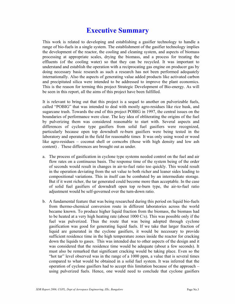
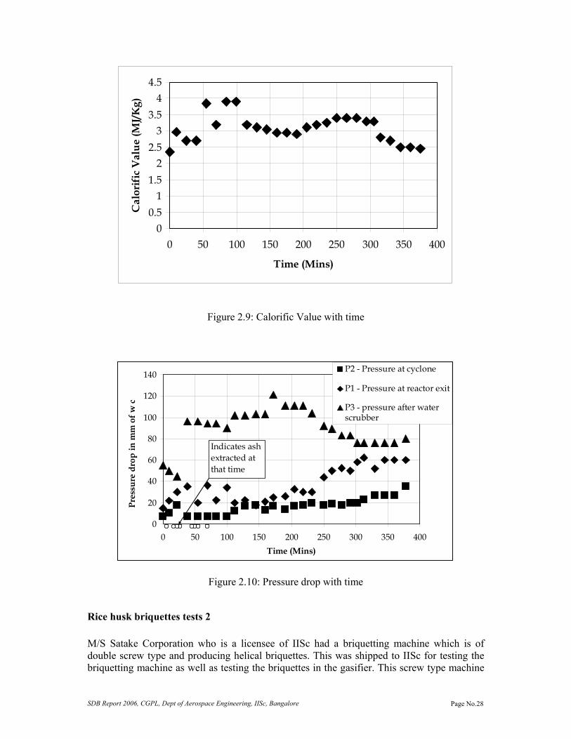
The gas composition averaged like CO ~ 14 ± 1, H2 ~ 14 ± 1, CH4 ~ 3 ± 1, CO2 ~ 17 ± 2 and rest N2. This is shown in Figure. 2.6. The rice husk briquette consumption on an averaged was 38 kg/hr. This is plotted in Figure. 2.7. The gas temperature at the reactor exit and cyclone exit is plotted in Figure. 2.8. The gas temperatures are stable from 180 minutes of operation. The calorific value of gas is around 3.0 ± 0.5. This is shown in Figure. 2.9. The variation in pressure drops across various gasification system elements is shown in Figure. 2.10.
-5
0
5
10
15
20
25
0 5 10 15 20 25 30
Time (Mins)
Gas
com
posi
tion(
%)
CH4
CO
H2
CO2
O2
Indicates ashextracted at that time
Figure 2.6: Gas Composition with time

SDB Report 2006, CGPL, Dept of Aerospace Engineering, IISc, Bangalore Page No.27
0
50
100
150
200
250
300
0 50 100 150 200 250 300 350 400
Time (Mins)
Bio
mas
s co
nsum
ptio
n C
umm
ulat
ive,
kg
38 kg/hr
Figure 2.7: Biomass Composition with time
0
100
200
300
400
500
600
700
0 100 200 300 400
Time (Mins)
Tem
pera
ture
(deg
C)
T1 at Reactor exit
T2 at Cyclone exit
Figure 2.8: Gas temperature with time
SDB Report 2006, CGPL, Dept of Aerospace Engineering, IISc, Bangalore Page No.28
00.5
11.5
22.5
33.5
44.5
0 50 100 150 200 250 300 350 400
Time (Mins)
Cal
orif
ic V
alue
(MJ/
Kg)
Figure 2.9: Calorific Value with time
0
20
40
60
80
100
120
140
0 50 100 150 200 250 300 350 400Time (Mins)
Pres
sure
dro
p in
mm
of w
c
P2 - Pressure at cyclone
P1 - Pressure at reactor exit
P3 - pressure after waterscrubber
Indicates ash extracted at that time
Figure 2.10: Pressure drop with time
Rice husk briquettes tests 2 M/S Satake Corporation who is a licensee of IISc had a briquetting machine which is of double screw type and producing helical briquettes. This was shipped to IISc for testing the briquetting machine as well as testing the briquettes in the gasifier. This screw type machine

SDB Report 2006, CGPL, Dept of Aerospace Engineering, IISc, Bangalore Page No.29
was different from the one procured in the project earlier where the barrel was heated to 300 0C, but in the Japanese machine the barrel was cooled by circulating water in the jacket. The new briquetting machine involved two stage briquetting in which the first screw of large taper pulverized the rice husk against a cogged wall and the second screw which had little taper briquetted it. The second screw had a barrel with water jacket. The rice husk was briquetted in the new screw type briquetting machine. The gasifier was run with these briquettes. The briquettes were spiral in shape and had an intrinsic density of 1000 kg/m3.
Tests The tests were carried on the 80 kg/hr gasification system. The system was freshly loaded with charcoal and wood and later flushed with rice husk briquettes. The system was run till the briquettes burning being seen in the nozzles. The next day the system was restarted and run for 12 hours and various measurements made.
Important observations It was observed that the ash extraction rate effected the gasifier operation causing a drastic change in the gas composition, which called for an optimization of the process. It was decided that for every batch of loading there would be an equivalent amount of ash extracted (say 20% of loading). Voids were observed during the run that were attributed to non-uniform flow of material.
Plate 2 RiceHusk Briquette (White)
Dimension L=35mm ; B=18mm ; Ht.=22mm Density ~ 1000 kg/m3. Bulk density > 480 kg/m3. Ash Content 20%

SDB Report 2006, CGPL, Dept of Aerospace Engineering, IISc, Bangalore Page No.30
Though considerable tar was observed separated in the chilled water scrubber thus displaying the effectiveness of chilled water, no tar was observed in the bubbling column of anisole through the entire run. The gas composition was found to be around CO ~ 15 ± 1 %, H2 ~ 12 ± 2 %, CH4 ~ 1.8 ± 0.3, CO2 ~ 15 ± 1% and N2 – rest. This has been presented in Figure. 2.11. The gas flow rate is maintained around 18 g/s as shown in Figure. 2.12 and corresponding biomass consumption is around 10 kg/hr as shown in Figure. 2.13. The gas temperature at reactor exit (T1) and cyclone exit (T2) is plotted in Figure. 2.14. The T1 temperature has a raising and falling trend between 600 and 700 0C. This is due to creation and clearance of voids. This can be taken care by further reducing the size of the briquettes before feeding into the reactor. The pressure drops across reactor (P1), after cyclone (P2), after scrubber 1 (P3) and after chill scrubber (P4) have shown in increasing trend. The suction pressure with time is plotted in Figure. 2.15. This shows that 20% extraction is not adequate and slightly higher extraction has to be adopted.
02468
1012141618
0 100 200 300 400 500 600 700
Time in Mins
Gas
Com
posi
tion
(%)
CO
CO2
CH4O2
H2
Figure 2.11: Gas Composition with time

SDB Report 2006, CGPL, Dept of Aerospace Engineering, IISc, Bangalore Page No.31
0
5
10
15
20
25
0 200 400 600 800
Time in mins
Gas
flow
rate
g/s
Figure 2.12: Gas flow rate with time
0
20
40
60
80
100
120
140
0 100 200 300 400 500 600 700
Time in mins
Cum
ulat
ive
Bio
mas
s lo
adin
g, k
g
30 kg/hr
Figure 2.13: Biomass Consumption with time

SDB Report 2006, CGPL, Dept of Aerospace Engineering, IISc, Bangalore Page No.32
0
100200
300
400
500600
700
800
0 100 200 300 400 500 600 700
Time in mins
Gas
Tem
pera
ture
deg
CT1
T2
Figure 2.14: Gas Temperature with time
0
50
100
150
200
250
300
350
0 100 200 300 400 500 600 700Time in mins
Stat
ic P
ress
ure
mm
wg
P1P2P3P4
Figure 2.15: Pressure drop with time
SDB Report 2006, CGPL, Dept of Aerospace Engineering, IISc, Bangalore Page No.33
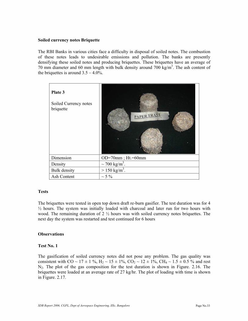
Soiled currency notes Briquette The RBI Banks in various cities face a difficulty in disposal of soiled notes. The combustion of these notes leads to undesirable emissions and pollution. The banks are presently densifying these soiled notes and producing briquettes. These briquettes have an average of 70 mm diameter and 60 mm length with bulk density around 700 kg/m3. The ash content of the briquettes is around 3.5 – 4.0%.
Tests The briquettes were tested in open top down draft re-burn gasifier. The test duration was for 4 ½ hours. The system was initially loaded with charcoal and later run for two hours with wood. The remaining duration of 2 ½ hours was with soiled currency notes briquettes. The next day the system was restarted and test continued for 6 hours
Observations Test No. 1 The gasification of soiled currency notes did not pose any problem. The gas quality was consistent with CO ~ 17 ± 1 %, H2 ~ 15 ± 1%, CO2 ~ 12 ± 1%, CH4 ~ 1.5 ± 0.5 % and rest N2. The plot of the gas composition for the test duration is shown in Figure. 2.16. The briquettes were loaded at an average rate of 27 kg/hr. The plot of loading with time is shown in Figure. 2.17.
Plate 3 Soiled Currency notes briquette
Dimension OD=70mm ; Ht.=60mm Density ~ 700 kg/m3. Bulk density > 150 kg/m3. Ash Content ~ 5 %

SDB Report 2006, CGPL, Dept of Aerospace Engineering, IISc, Bangalore Page No.34
Test No. 2 The gasification did not pose any problem excepting that ash extraction had to be done for longer duration owing to lightness of the briquette char. The gas composition essentially remained same with CO + H2 remaining about same and marginal increase in CH4. The plot of gas composition with time for the test duration is shown in Figure. 2.18. The average loading of the briquette was 2 kg/hr as shown in Figure. 2.19. The gas calorific value was around 3.5 to 4.0 MJ/nm3 during the latter part of the test as shown in Figure. 2.20.
0
5
10
15
20
25
30
170 190 210 230 250 270 290
Time in minutes
Gas
com
posi
tion,
% CO
CO2CH4O2
H2
Figure 2.16: Gas Composition with time in the first test
0
20
40
60
80
100
120
0 50 100 150 200 250 300
Time in minutes
Bio
mas
s lo
aded
, kg
s
Average biomass loaded 27 kg/hr
Figure 2.17: Average biomass consumption with time in the first test

SDB Report 2006, CGPL, Dept of Aerospace Engineering, IISc, Bangalore Page No.35
0
5
10
15
20
0 100 200 300 400
Time in mins
Gas
com
posi
tion,
%
COCO2
CH4O2
H2
Figure 2.18: Gas Composition with time in the second test
020406080
100120140160
0 100 200 300 400
Time in mins
Bio
mas
s lo
aded
, kgs
Average biomass consumption 23
kg/hr
Figure 2.19: Biomass consumption with time in the second test

SDB Report 2006, CGPL, Dept of Aerospace Engineering, IISc, Bangalore Page No.36
2.502.702.903.103.303.503.703.904.10
0 100 200 300 400
Time in mins
Cal
val
ue M
J/kg
Figure 2.20: Gas Calorific Value with time in the second test
Pine Needle Briquette testing The pine needle briquettes were tested in the 10 kg/hr gasification system. The briquettes were produced in a ram type briquetting machine and had a briquette density of 850 kg/m3 and bulk density of 350 kg/m3. The ash content of the briquettes was found to be 5%. The test duration was for 3½ hour with average briquette consumption of 8 kg/hr and gasification of pine needle briquettes posed no problems. The results of the tests are summarized in the Table 2.5 and the experimental setup is shown in Plates 5 to 7.
Plate 4 Pine Needle Briquette
Dimension OD=50mm ; Ht.=50mm Density ~ 850 kg/m3. Bulk density > 600 kg/m3. Ash Content 2.7%

SDB Report 2006, CGPL, Dept of Aerospace Engineering, IISc, Bangalore Page No.37
Table 2.5: Summary of Pine needle Briquette test
Time mins
Reactor Pr, mmwg
CO %
CO2 %
H2 %
O2 %
CH4
% Briquettes loaded, kg
0 0 0 0 0 0 0 Topping with 5 kgs
30 54 10 60 57 16.7 8.0 10.4 0.6 0.8 90 68 19.6 6.3 11.4 0.4 0.4
120 95 17.0 7.2 12.6 1.5 1.0 7 180 5 210 5
Plate 5: 10 kg/hr gasifier with pine needle briquette Plate 6: Producer gas being flared
Plate 7: Pine needle briquettes kept ready for loading

SDB Report 2006, CGPL, Dept of Aerospace Engineering, IISc, Bangalore Page No.38
Coir Pith Briquette testing Coir pith is obtained from coconut husk mainly during the process of fiber making. Extraction of 1 kg of coir generates 2 kg of coir pith. This has a high lignin (31%) and cellulose (27%) content and a carbon-nitrogen (C/N) ratio of 104:1. This also has a high water carrying capacity (~ 5 to 6 times its weight). The high lignin content prevents early decomposition and the same lignin helps in briquetting without any additional binder. The process of briquetting calls for reducing the moisture content from nearly 50% on wet basis to less than 10%. The process of fiber making, where the husk is soaked in water and taken for further processing, makes coir pith to have a high degree of acquired moisture. This cannot be dried by sun-drying alone and requires a dryer. One such dryer that can dry this loose biomass is rotary dryer. The dried pith has a low bulk density of 80 – 100 kg/m3 and has to be briquetted before using in gasifier. This can be achieved by using ram type briquetting machine. The coir pith briquettes that were produced were of 50 mm in diameter and were cut to 40 mm pieces for gasification. The briquetting machine consumed about 9 kWe of power while briquetting around 125 kg/hr coir pith. The intrinsic density of these briquettes was greater than 950 kg/m3 and bulk density greater than 350 kg/m3. The ash content of these briquettes was around 8%. A reverse down draft gasification stove experiment was conducted to observe any ash fusion. No clinker formation was observed till superficial velocity of 0.3 m/s. The ash collected from above test was sent for analysis and the ash composition is shown in Table 2.6.
Table 2.6: Chemical Composition of Coir Pith ash
Sl. No Chemical Species Fraction, %
1 Silica (SiO2) 9.8 2 Alumina (AL2O3) 0.6 3 Ferric Oxide (Fe2O3) 0.8 4 Titanium-di-Oxide (TiO2) 0.2 5 Calcium Oxide (CaO) 2.7 6 Magnesium Oxide (MgO) 4.4 7 Sodium Oxide (Na2O) 12.1 8 Potash (K2O) 15.4 9 Loss on Ignition 45.6 10 Water Soluble Chloride 8
Tests The coir pith briquette was tested on 80 kg/hr gasifier for duration of 2 ½ hours. The system was initially loaded with charcoal and wood and later topped with coir pith briquettes. All the measurements were made after the briquettes were seen at the nozzles. The duration of briquette gasification was for 1 ½ hour.

SDB Report 2006, CGPL, Dept of Aerospace Engineering, IISc, Bangalore Page No.39
Observations The gasification of coir pith did not pose any problem. The gas composition averaged around CO ~ 16.5%, H2 ~ 7.5%, CH4 ~ 0.2%, CO2 ~ 12.3% and rest nitrogen. The plot of gas composition with time is shown in Figure. 2.21. The average briquette consumption was 44 kg/hr as shown in Figure. 2.22. The pressure drop across the reactor was within the designed limit as shown in Figure. 2.23.
0
5
10
15
20
0 10 20 30 40 50 60 70
Time in mins
Com
posi
tion
in % CO
CO2 H2
CH4
Figure 2.21: Gas composition with time
0
20
40
60
80
100
0 20 40 60 80 100 120 140
Time in mins
Bio
mas
s lo
aded
in k
gs
Average 44 kg/hr
Figure 2.22: Biomass Consumption with time

SDB Report 2006, CGPL, Dept of Aerospace Engineering, IISc, Bangalore Page No.40
0
20
40
60
80
100
0 20 40 60 80 100 120 140
Time in mins
Rea
ctor
Pre
ssur
e dr
op,
mm
wg
Figure 2.23: Reactor pressure drop with time
Saw Dust briquette testing M/S Hindustan Pencils are leading pencil manufacturers. They have two factories in Jammu and two in other locations. The two units at Jammu rely on a large extend to in-house power generation which was basically generated by diesel engine-generator sets. The factory also had problem of disposing the sawdust which was generated in the process of pencil manufacture in various stage. To some extent this dust was utilized in boiler for steam generation for dryer operations, the remaining was briquetted in a ram type briquetting machine and stored. The characteristic of the briquette is shown below.
Characteristic of Saw dust Briquette
Plate 7 The Saw dust Briquette
Dimension OD=50mm ; Ht=35mm
Density ~ 1000 kg/m3 Bulk density > 500 kg/m3 Ash Content 3%

SDB Report 2006, CGPL, Dept of Aerospace Engineering, IISc, Bangalore Page No.41
The factory decided to install IISc open top down draft gasifier. In order to evaluate the performance of these briquettes nearly 1 tonne of briquettes were obtained for testing. Performance Tests The briquettes were sized to 60 mm diameter X 30 mm length and fragmented pieces were discarded. Trials were conducted both in burner mode and on gas engine mode, the G743G engine which was in the laboratory for 100 hour testing. Test results on engine mode Table 2.7 contains the operational summary of the test with gas engine. The total duration of the test with this briquette was for 13 hours with split operations of 6 hours and 7 hours on two days. The gasifier was operating with wood as a part of the standard 100 hour test planned for evaluating G743G Cummins Gas engine. The briquettes were loaded in between and the system was operated. An overnight shutdown was also planned to understand the behavior of the briquettes upon cooling and subsequent start-up. The system was restarted after 16 hours overnight stoppage, no clinker or additional pressure drop was seen. The plot of pressure drop with time is shown in Figure. 2.24. The gas composition was consistent and is shown in Figure. 2.25. The Calorific value was around 4.5 ± 0.3 MJ/kg as shown in Figure. 2.26.
Table 2.7: Summary of Cummins gas engine operations using saw dust briquettes Load kWe
Duration of operation in
hours
Biomass consumed
in kgs
Avg. Gas flow from
venturi
Specific biomass
consumption per kWh
Frequency Exhaust oxygen
No 2 80 31 g/s - - ~ 2% 20 1 50 41 g/s 2.5 50.4 ~ 1.6% 40 1.5 86 50 g/s 1.4 49.9 ~ 1.4% 50 45 mins 50 54 g/s 1.3 48.6 ~ 1.8%
-250
-200
-150
-100
-50
00 5 10 15 20 25 30 35
Time in Hours
Rea
ctor
Pre
ssur
e dr
op m
mw
g
16 hours overnight shut down
Figure 2.24: Reactor pressure drop with time

SDB Report 2006, CGPL, Dept of Aerospace Engineering, IISc, Bangalore Page No.42
0
5
10
15
20
25
0 100 200 300 400
Time in mins
Gas
Com
posi
tion
% CO
H2
CO2 CH4 O2
Figure 2.25: Gas Composition with time
0
1
2
3
4
5
6
0 100 200 300 400
Time in mins
Cal
orif
ic V
alue
MJ/
kg
Figure 2.26: Gas Calorific Value with time Field System A 300 kg/hr gasification system was designed and implemented by a manufacturer (M/S BETEL) who holds a license from IISc. The system was designed to handle briquettes and was designed as per industrial standards. The reactor was lined with 99% Alumina bricks in the oxidation and reduction zone and for 1 m above it. A second stage cyclone was incorporated in series to take care of any additional particulate loading. Two water scrubbers and a chilled water scrubber along with fabric filter formed the cooling and cleaning system. Biomass loading arrangement and water treatment system was the auxiliary to the gasification plant to make it more operation friendly. The start-up and shut down was automated using sequential timer. The gasification plant at M/S Hindustan Pencils is shown in Plate 8.

SDB Report 2006, CGPL, Dept of Aerospace Engineering, IISc, Bangalore Page No.43
Plate 8: Gasification Plant at M/S Hindustan Pencils
Plant operations The system was initially operated in dual fuel mode substituting diesel in the diesel engines at the factory. In the second phase, naturally aspirated gas engines of 80 kWe and 160 kWe capacities on producer gas have been added. The month wise plant operation data is shown in Table 2.8.

SDB Report 2006, CGPL, Dept of Aerospace Engineering, IISc, Bangalore Page No.44
Table 2.8: Month wise operational details Month Operation
hours Biomass
consumed kg kWh
generated kWh
exportedRemarks
July 2003 79 7818 6629 4970 System commissioned Aug. 2003 323 32032 24101 17318 Breakage of ‘CUMI’
central air nozzle, replaced with SS 316 L air nozzle
Sept. 2003 442 49031 54696 44973 Fabric filter choking in 40 hours
Oct. 2003 498 54475 66321 57198 Nov. 2003 369 37249 50220 44320 200 kVA and 380 kVA
engines run Dec. 2003 310 33433 50532 44925 Turbochargers of the
above two engines failed
Jan. 2004 214 21417 36120 32006 After cooler blocked and cleaned partially
Feb. 2004 246 28962 40056 34871 380 kVA turbocharger failed
Mar. 2004 317 38373 48384 41419 April 2004 370 47971 56988 49134
The operations beyond May 2004 are averaging around 350 - 400 hours per month.
Gas quality measurements After the receiving report that turbocharger had failed twice a visit was made to the plant in the month of June 2003. The operations were observed and following operational problems were uncovered:
• The quality of briquettes had deteriorated and loading of high density biomass/ charcoal during shut down not properly adhered. Bloating of briquettes at the top due to condensate water absorption observed leading to deterioration in gas quality.
• The water flow rate measured at scrubbers was lower than designed which led to losing of cooling and cleaning efficiency.
• A few fabric bags were not clamped properly to cartridge leading to short circuiting of particles into the engine.
• The pipe line laid by the factory to the dual fuel engines did not have adequate flanges for cleaning. The method adopted to clean the long tubes lead to mound of dust collected in the floor at the middle of the pipe.
After correcting the above mistakes, the system was run and gas analysis was made. Table 2.9 shows the result of the gas analysis.
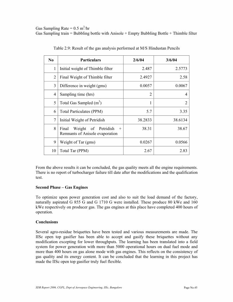
SDB Report 2006, CGPL, Dept of Aerospace Engineering, IISc, Bangalore Page No.45
Gas Sampling Rate = 0.5 m3/hr Gas Sampling train = Bubbling bottle with Anisole + Empty Bubbling Bottle + Thimble filter
Table 2.9: Result of the gas analysis performed at M/S Hindustan Pencils
No Particulars 2/6/04 3/6/04
1 Initial weight of Thimble filter 2.487 2.5773
2 Final Weight of Thimble filter 2.4927 2.58
3 Difference in weight (gms) 0.0057 0.0067
4 Sampling time (hrs) 2 4
5 Total Gas Sampled (m3) 1 2
6 Total Particulates (PPM) 5.7 3.35
7 Initial Weight of Petridish 38.2833 38.6134
8 Final Weight of Petridish + Remnants of Anisole evaporation
38.31 38.67
9 Weight of Tar (gms) 0.0267 0.0566
10 Total Tar (PPM) 2.67 2.83 From the above results it can be concluded, the gas quality meets all the engine requirements. There is no report of turbocharger failure till date after the modifications and the qualification test. Second Phase – Gas Engines To optimize upon power generation cost and also to suit the load demand of the factory, naturally aspirated G 855 G and G 1710 G were installed. These produce 80 kWe and 160 kWe respectively on producer gas. The gas engines at this place have completed 400 hours of operation. Conclusions Several agro-residue briquettes have been tested and various measurements are made. The IISc open top gasifier has been able to accept and gasify these briquettes without any modification excepting for lower throughputs. The learning has been translated into a field system for power generation with more than 5000 operational hours on dual fuel mode and more than 400 hours on gas alone mode with gas engines. This reflects on the consistency of gas quality and its energy content. It can be concluded that the learning in this project has made the IISc open top gasifier truly fuel flexible.

SDB Report 2006, CGPL, Dept of Aerospace Engineering, IISc, Bangalore Page No.46
Chapter III Biomass Gasification systems for High Grade Thermal Application in the Industrial Sector Introduction The high temperature application is for a heat treatment industry, namely M/s TamilNadu Heat Treaters and Fettling Services (TAHAFET) located in Hosur, TamilNadu. The industry has eight furnaces and offers services like; heat treatment and fettling to the castings and forging units, 300 days in a year all round the clock. Prior to the introduction of gasifiers, the industry used Light Diesel Oil (LDO) for operating its eight furnaces with temperatures in the range of 600 to 920 C. Figure 3.1 shows the fossil fuel system connected to the furnace. The consumption of LDO was 2000 liter/day averaging about 1200 kWth.
Figure 3.1: Fossil fuel system for high temperature application The LDO fired system consisted of two burners to each of the furnace, with temperature controlled by a PID controller. The required air to fuel ratio is attained using a Ratiotrol which operates on the principle of balancing the pressure using a pressure regulator. Every batch of stock- forging/casting loaded into the furnace undergoes a heating cycle involving initial heating and soaking operations. These operations are pre-programmed and controlled by a PID controller. A gasifier of 300-kg/hr capacity, similar in configuration described in chapter 1 is retrofitted to eight furnaces. The novelty in this package is the use of one gasifier system to energize eight furnaces requiring different operation temperatures. This has been possible by using a ratio controller (ratiotrol) on individual furnace so as to maintain the air to fuel ratio; with control parameter being the furnace temperature. Two burners are provided for each of the furnace, thus a total of sixteen burners combust producer gas generated from the gasifier.

SDB Report 2006, CGPL, Dept of Aerospace Engineering, IISc, Bangalore Page No.47
With the use of pressure regulator and ratiotrol on the gas line to attain the air-fuel ratio, the demand for superior quality gas is high; comparable to the one expected for an internal combustion engine – contaminants around 50 ppm level. Therefore the gas cleaning system in this package is more rigorous compared to the one for the drying application The system is configured with a PLC to carry out operations related to ash extraction, fuel feeding and other safety regulatory measures for the system. All the data with respect to pressure and temperature are logged continuously on to a computer. Schematic of the gasification system addressing the high temperature application is as shown in Figure. 3.2.
TOP COVER{ OPEN DURING OPERATION }
REACTOR
ASH EXTRACTION SYSTEM
CYCLONE
DIRECT COOLINGSYSTEM
COOLINGTOWER
PR. SANDBED FILTER
ACTIVATED CARBON FILTER
WATER SUMP
SCRUBBER
BLOWER 1
START UPFLARE
WATER LINE
GAS LINE
DIESEL SCRUBBER
BOOSTER BLOWER
FURNACES
1 2 3 4 5 6 7 8
Figure 3.2: Schematic of the 300 kg/hr gasifier system
Performance Producer gas from the gasifier system is available at a pressure of 10000 Pa (gauge) at the blower exit, which is also the operational pressure for the ratiotrol. The burner nozzle dimension has been suitably chosen so as to provide necessary amount of gas into the burner, without much modifications in the liquid fuel system. This aspect provides an advantage for the industry to switch over to the liquid fuel system in case of biomass non-availability or gasifier maintenance. Table 3.1 shows the details on the performance of the furnaces using light diesel oil (LDO) and producer gas as the fuel. The consumption of LDO was about 2000 litre/day. Of the eight furnaces, five operate at 900 0C and the remaining at 600 0C. From the data presented in the table, the time taken by the producer gas operation is about 25% excess as compared to the LDO based operation. This probably is true because the radiation from the liquid flame would be higher than that of gaseous flame. The liquid fuel upon combustion is generally seen with a yellowish sooty flame in comparison to nearly colorless gas combustion. Further the peak temperature achieved with liquid fuel combustion system is higher than PG operation.
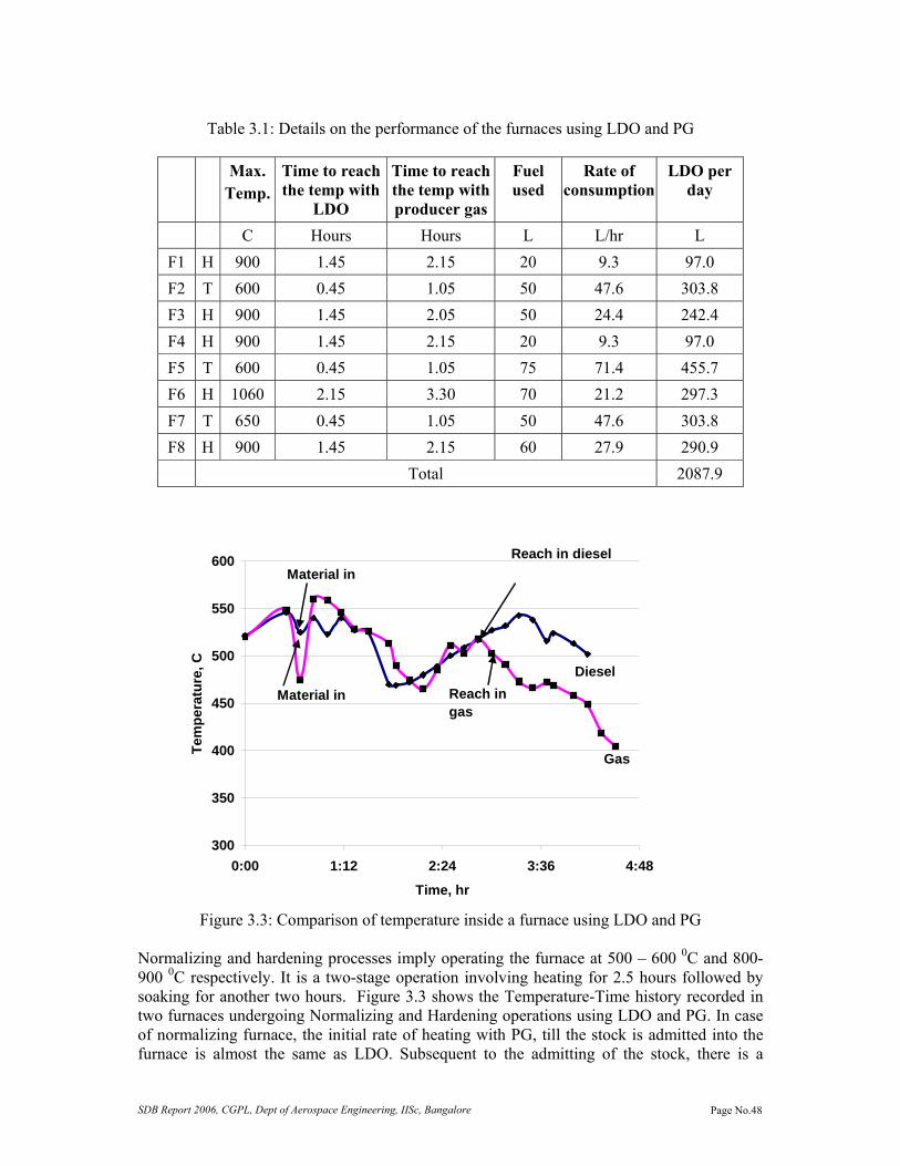
SDB Report 2006, CGPL, Dept of Aerospace Engineering, IISc, Bangalore Page No.48
Table 3.1: Details on the performance of the furnaces using LDO and PG
Max.
Temp.Time to reach the temp with
LDO
Time to reach the temp with producer gas
Fuel used
Rate of consumption
LDO per day
C Hours Hours L L/hr L F1 H 900 1.45 2.15 20 9.3 97.0 F2 T 600 0.45 1.05 50 47.6 303.8 F3 H 900 1.45 2.05 50 24.4 242.4 F4 H 900 1.45 2.15 20 9.3 97.0 F5 T 600 0.45 1.05 75 71.4 455.7 F6 H 1060 2.15 3.30 70 21.2 297.3 F7 T 650 0.45 1.05 50 47.6 303.8 F8 H 900 1.45 2.15 60 27.9 290.9
Total 2087.9
300
350
400
450
500
550
600
0:00 1:12 2:24 3:36 4:48
Time, hr
Tem
pera
ture
, C Diesel
Gas
Material in
Material in Reach in gas
Reach in diesel
Figure 3.3: Comparison of temperature inside a furnace using LDO and PG
Normalizing and hardening processes imply operating the furnace at 500 – 600 0C and 800-900 0C respectively. It is a two-stage operation involving heating for 2.5 hours followed by soaking for another two hours. Figure 3.3 shows the Temperature-Time history recorded in two furnaces undergoing Normalizing and Hardening operations using LDO and PG. In case of normalizing furnace, the initial rate of heating with PG, till the stock is admitted into the furnace is almost the same as LDO. Subsequent to the admitting of the stock, there is a
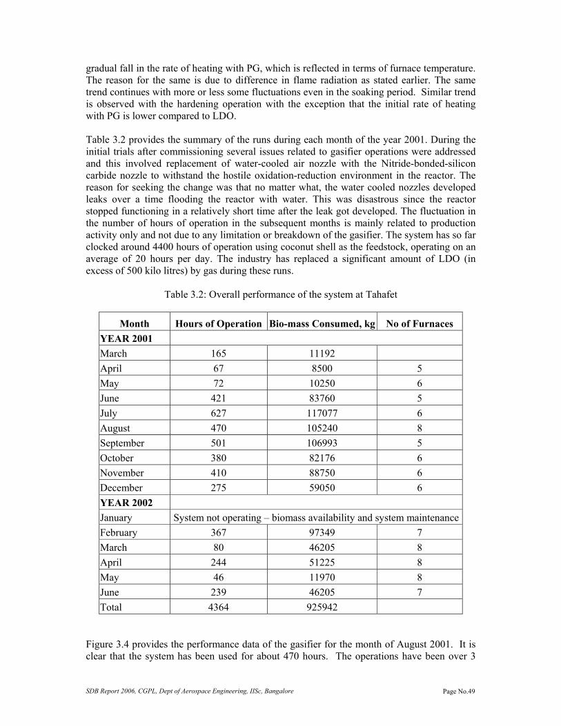
SDB Report 2006, CGPL, Dept of Aerospace Engineering, IISc, Bangalore Page No.49
gradual fall in the rate of heating with PG, which is reflected in terms of furnace temperature. The reason for the same is due to difference in flame radiation as stated earlier. The same trend continues with more or less some fluctuations even in the soaking period. Similar trend is observed with the hardening operation with the exception that the initial rate of heating with PG is lower compared to LDO. Table 3.2 provides the summary of the runs during each month of the year 2001. During the initial trials after commissioning several issues related to gasifier operations were addressed and this involved replacement of water-cooled air nozzle with the Nitride-bonded-silicon carbide nozzle to withstand the hostile oxidation-reduction environment in the reactor. The reason for seeking the change was that no matter what, the water cooled nozzles developed leaks over a time flooding the reactor with water. This was disastrous since the reactor stopped functioning in a relatively short time after the leak got developed. The fluctuation in the number of hours of operation in the subsequent months is mainly related to production activity only and not due to any limitation or breakdown of the gasifier. The system has so far clocked around 4400 hours of operation using coconut shell as the feedstock, operating on an average of 20 hours per day. The industry has replaced a significant amount of LDO (in excess of 500 kilo litres) by gas during these runs.
Table 3.2: Overall performance of the system at Tahafet
Month Hours of Operation Bio-mass Consumed, kg No of Furnaces YEAR 2001 March 165 11192 April 67 8500 5 May 72 10250 6 June 421 83760 5 July 627 117077 6 August 470 105240 8 September 501 106993 5 October 380 82176 6 November 410 88750 6 December 275 59050 6 YEAR 2002 January System not operating – biomass availability and system maintenanceFebruary 367 97349 7 March 80 46205 8 April 244 51225 8 May 46 11970 8 June 239 46205 7 Total 4364 925942
Figure 3.4 provides the performance data of the gasifier for the month of August 2001. It is clear that the system has been used for about 470 hours. The operations have been over 3

SDB Report 2006, CGPL, Dept of Aerospace Engineering, IISc, Bangalore Page No.50
weeks, with nearly continuous mode of using the gasifier. The average biomass consumption has been between 5 to 6 tons per day. The non-operational days is linked to production activity or non-availability of biomass. During this month, all the furnaces have been in operation and about 105 tons of biomass has been used to replace about 26 kilo liters of LDO (4 kg/litre on an average). It is legitimate to bring out here as to how the nature of fuel affects the quality of the end product. The liquid fuel system is designed to operate with excess air in order to ensure complete combustion. Therefore the excess oxygen present in the flue gas at elevated temperature (~ 600 C and above) resulted in oxidation of the material being heat-treated thus resulting in poor surface finish and weight loss of the end product. The presence of sulphur in the fuel also resulted in eroding the surface other escaping as SO2. In contrast the PG operation has been found to be extremely clean without any smoke. Since the PG combustion occurs close to stoichiometry the surface finish has been found to be good without any surface oxidation.
Performance of the system at Tahafet for the month of August
01000200030004000500060007000
1/8/
2001
3/8/
2001
5/8/
2001
7/8/
2001
9/8/
200
11/8
/200
1
13/8
/200
1
15/8
/200
1
17/8
/200
1
19/8
/200
1
21/8
/200
1
23/8
/200
1
25/8
/200
1
27/8
/200
1
29/8
/200
1
31/8
/200
1
kg o
f bio
mas
s pe
r day
Performance of the system at Tahafet for the
month of August
-1
4
9
14
19
24
1/8/
2001
3/8/
2001
5/8/
2001
7/8/
2001
9/8/
200
11/8
/200
1
13/8
/200
1
15/8
/200
1
17/8
/200
1
19/8
/200
1
21/8
/200
1
23/8
/200
1
25/8
/200
1
27/8
/200
1
29/8
/200
1
31/8
/200
1Hou
rs o
f ope
ratio
n pe
r day
Figure 3.4: Performance data for the month of August 2001
Conclusions Trails and performance of the plant is synthesized in this section. The performance is presented in terms of quantum of fossil fuel substituted, which reflects on the extent of foreign exchange saved and the reduction in GHG emissions. The number of hours of operation reflects the operation reliability of the plant. An important parameter is also arrived that reflect the overall performance of the gasifier system in terms of amount of biomass required to replace one litre of diesel. This index has a bearing on the economics of operation.

SDB Report 2006, CGPL, Dept of Aerospace Engineering, IISc, Bangalore Page No.51
Chapter IV Development of Power Package for Plastic Residues and Effluents from the Industrial and Urban Wastes Introduction Twentieth century has seen quantum growth in path breaking technology and industrialization. This growth, while beneficial to humanity, has had its impact on the environment. Most developed nations have achieved a high rate of industrial growth, with inadequate respect for environmental issues, a policy decision that is now undergoing a rethinking of priorities. The need for effective disposal of huge volumes of industrial waste is becoming more challenging due to expected imposition of stringent pollution control regulations in the near future. Thermo chemical conversion, particularly gasification of organics in the waste is considered the best route from the perspective of volume reduction and prevalent eco-friendly concept of waste-to-energy transformation. It is considered imperative to have adequate understanding of basic combustion features as a part of the thermo-chemical conversion process, leading to gasification. The aim of this work is to understand the fundamental combustion processes associated with one of the top listed hazardous wastes from distilleries (Biochemical Oxygen Demand (BOD) ~ 40,000 – 50,000 mg/L), commonly known as vinasse, stillage or spent wash, through experiments and modeling efforts. Specially designed experiments on distillery effluent combustion and gasification are conducted in laboratory scale reactors. Single droplet studies on distillery effluents As an essential starting point of the studies on ignition and combustion of distillery effluent containing solids consisting of 62±2% organics and 38±2% inorganics (primarily sugarcane derivatives), the roles of solids concentration, drop size and ambient temperature were investigated through experiments on (1) liquid droplets of 65% and 77% solids (remaining water) and (2) spheres of dried effluent (100% solids) of size 0.5 mm to 20 mm diameter combusted at ambient temperatures of 773 to 1273 K. The investigation reveals that the droplets burn with two distinct regimes of combustion, flaming and char glowing. The ignition delay ‘ti’ of the droplets increased with size as is in the case of non-volatile droplets, while that of bone-dry spheres was found to be independent of size. The ‘ti’ decreased with increase in solids concentration. The ignition delay has showed an Arrhenius dependence on temperature. The initial ignition of the droplets and the dry spheres led to either homogeneous (flaming) or heterogeneous (flameless) combustion, depending on the ambient temperature in the case of sphere and on solid concentration and the ambient temperature, in the case of liquid droplets. The weight loss during the flaming combustion was found to be 50-80% while during the char growing it was 10-20% depending on the ambient temperature. The flaming time ‘tf’ is observed as 2
0~ dt f , as in the case of liquid fuel droplets and wood
spheres. The char glowing time ‘tc’ is observed as 2~ cdtc as in the case of wood char, though the inert content of effluent char is as large as 50% compared to 2-3% in wood char. In the case of initial flameless combustion, the char combustion rate is observed to be lower.

SDB Report 2006, CGPL, Dept of Aerospace Engineering, IISc, Bangalore Page No.52
Experiments on gasifying distillery Effluents Based on the results of single droplet combustion studies, combustion experiments were conducted in a laboratory scale vertical reactor (throughput ranging from 4 to 10 g/s) with the primary air of obtaining sustained combustion. Spray of effluents with 50% and 60% solids (calorific value 6.8 -8.2 MJ/kg), achieved by an air blast atomizer, was injected into a hot oxidizing environment to determine the parameters (ambient temperature and air-fuel ratio) at which auto-ignition could occur and subsequently studies were continued to investigate pre-ignition, ignition and combustion processes. Effluent with lower solids concentration was considered first from the point of view of the less expensive evaporator required in the field conditions for concentration and a spin-off in terms of better atomization consequently. Three classes of experiments were conducted: 1) Effluent injection from the wall with no auxiliary heat input, 2) Effluent injection with auxiliary heat input and 3) effluent injection within kerosene enveloping flame. Though individual particles in the spray periphery were found to combust, sustained spray combustion was not achieved in any of the three sets of experiments even with fine atomization. While conducting the third class of experiments in an inclined metallic reactor, sustained combustion of the pool resulting of accumulated spray seemed to result in large conversion of carbon. This led to the adoption of a new concept for effluent combustion in which the residence time is controlled by varying reactor inclination and the regenerative heat transfer from the product gases supplied heat for endothermic pre-ignition process occurring on the bed. Combustion and gasification experiments were conducted in an inclined plate reactor with rectangular cross section (80 mm x 160 mm) and 3000 mm long. A support flame was found necessary in the injection zone in addition to the regenerative heat transfer. Effluent with 60% solids was injected as film on the reactor bed. These films disintegrated into fine particles due to induced aerodynamic stretching and shear stripping. Combustion of individual particles provided exothermic heat profile and resulted into high carbon conversion. However, effluent clogging in the cold zone hindered system from attaining steady state. Effluent injected directly on the hot zone caused it to remain mobile due to the spheroidal evaporation and thus assuaging this problem. Improved mass distribution was achieved by displacing nozzle laterally in a cycle, actuated by a mechanism. Consistent injection led to sustained effluent combustion with resulting carbon conversion in excess of 98%. The typical gas fractions obtained during gasification condition (air ratio = 0.3) were CO2=14.0%, CO = 7.0%, H2=12.9%, CH4= 1%, H2S = 0.6-0.8% and about 2% of saturated moisture. This composition varied due to variation in temperature (±30K) and is attributed to combined effort of local flow variations, shifting zones of endothermic processes due to flowing of evaporating effluent over a large area. In order to minimize this problem, experiments were conducted by injecting effluent at higher solids (73% solids is found injectable). The effluent was found to combust closed to injection location due to the reduced ignition delay and lower endothermic evaporation load helped raising the local temperature. This caused the pyrolysis to occur in this hottest zone of the reactor with higher heating rates resulting in larger yield of devolatalized products and improved char conversion. Effluent combustion was found to sustain the temperature in the reactor under sub-stoichiometric conditions without support of auxiliary heat input and achieved high carbon conversion. These results inspire the use of higher concentration effluents, which is also known in the case of a wood to have improved gasification efficiency due to reduction in moisture fraction. In addition, the recent study on the sulfur emission in the case of black liquor combustion and recovery boilers have revealed that with increase in solids concentration, release of sulfur in gas phase reduces. The required concentration can be carried out using low grade waste heat
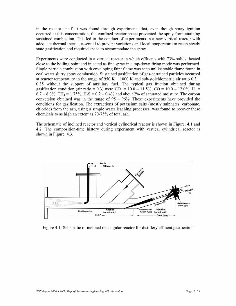
SDB Report 2006, CGPL, Dept of Aerospace Engineering, IISc, Bangalore Page No.53
in the reactor itself. It was found through experiments that, even though spray ignition occurred at this concentration, the confined reactor space prevented the spray from attaining sustained combustion. This led to the conduct of experiments in a new vertical reactor with adequate thermal inertia, essential to prevent variations and local temperature to reach steady state gasification and required space to accommodate the spray. Experiments were conducted in a vertical reactor in which effluents with 73% solids, heated close to the boiling point and injected as fine spray in a top-down firing mode was performed. Single particle combustion with enveloping faint flame was seen unlike stable flame found in coal water slurry spray combustion. Sustained gasification of gas-entrained particles occurred at reactor temperature in the range of 950 K – 1000 K and sub-stoichiometric air ratio 0.3 – 0.35 without the support of auxiliary fuel. The typical gas fraction obtained during gasification condition (air ratio = 0.3) were CO2 = 10.0 – 11.5%, CO = 10.0 – 12.0%, H2 = 6.7 – 8.0%, CH4 = 1.75%, H2S = 0.2 – 0.4% and about 2% of saturated moisture. The carbon conversion obtained was in the range of 95 – 96%. These experiments have provided the conditions for gasification. The extractions of potassium salts (mostly sulphates, carbonate, chloride) from the ash, using a simple water leaching processes, was found to recover these chemicals to as high an extent as 70-75% of total ash. The schematic of inclined reactor and vertical cylindrical reactor is shown in Figure. 4.1 and 4.2. The composition-time history during experiment with vertical cylindrical reactor is shown in Figure. 4.3.
Figure 4.1: Schematic of inclined rectangular reactor for distillery effluent gasification
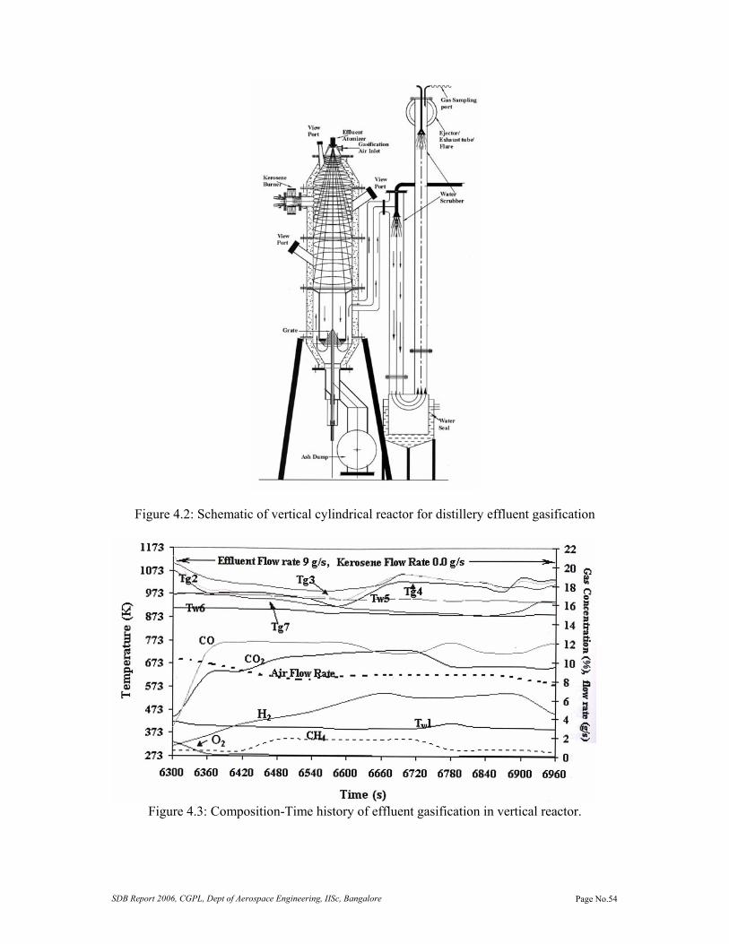
SDB Report 2006, CGPL, Dept of Aerospace Engineering, IISc, Bangalore Page No.54
Figure 4.2: Schematic of vertical cylindrical reactor for distillery effluent gasification
Figure 4.3: Composition-Time history of effluent gasification in vertical reactor.

SDB Report 2006, CGPL, Dept of Aerospace Engineering, IISc, Bangalore Page No.55
Dioxin Initially dioxin was an abbreviation for a single substance, with the formidable chemical name, 2,3,7,8-tetrachlorodibenzo-p-dioxin. It is one member of a "family" of chemical compounds with an identical carbon-oxygen framework. Chlorine atoms (four in this case) are attached at specific carbon atom sites as indicated by the numbers 2,3,7,8 in the name. The geometry of the molecule is shown in the figure below.
This pictorial shorthand describes the spatial relationship of the atoms that make up the molecule. How does the name relate to the structure? The di-benzo part comes from the two hexagons with inscribed circles. This is shorthand for benzene sub-structures. There is a carbon atom at the vertex of each hexagon.
The two benzene rings are joined by two oxygen atoms (5 and 10). By joining the benzene rings in this way the center of the molecule, containing the oxygens is also a six-membered ring. A six-membered ring like this with two oxygens in it is called dioxin. When the oxygens are at opposite sides of the ring, as in the figure, they are called para to each other, hence the -p- in the name. Two benzene rings joined with two oxygens in this fashion is dibenzo-p-dioxin, the so-called "parent" compound or structure or back-bone.
Toxicology studies of the effects of chlorinated dioxins on test animals indicate that the toxicity is not the same for each possible isomer (placement of chlorine around the molecule). Those isomers which contain chlorines in the 2,3,7, and/or 8 positions are more toxic than when hydrogen is attached to those positions. This led to using the term dioxin to describe all isomers of chlorinated dioxins containing from 1 to 8 (the maximum number) chlorines, and 2,3,7,8-dioxins to refer to the "toxic" isomers.
Pure 2,3,7,8-TCDD was synthesized in 1968. It is a white, micro-crystalline solid (looks like Table salt) which is insoluble in water and sparingly soluble in some organic solvents. 2,3,7,8-tetrachlorodibenzo-p-dioxin, Dioxin, also called Tetradioxin is denoted by its CAS number as : CAS Number: 1746-01-6; Its molecular formula is C12H4Cl402; Its molecular weight is, therefore, 321.96 and its melting point is 305 0C Dioxin generation during Combustion:
Combustion processes, where the fuel contains both carbon and chlorine, produce a wide range of dioxin isomers. It has also been discovered that above a certain temperature, however, (800 0C) dioxins are destroyed. It has been concluded that there is a natural background level of dioxins in the environment due to low temperature combustion events such as forest fires. This discovery produced some concern that people were at risk if they lived or worked near municipal incinerators, coal-fired power plants, home fireplaces, wood burning stoves, etc.

SDB Report 2006, CGPL, Dept of Aerospace Engineering, IISc, Bangalore Page No.56
Many of these possible sources have been studied, and the dioxin yield determined. As expected, low temperature combustion sources such as municipal incinerators produce higher levels of dioxins than the high temperature processes such as coal-fired power plants. All the levels found are in the part per trillion range or below. To simulate the release of dioxin during gasification, a trial was conducted using mix of standard biomass and tire pieces. Tire Gasification Experiment The other waste which is posing disposal problems and is in need of technological intervention for alternate use is municipal solid waste (MSW). There are certain towns where the municipal solid waste generation quantum is low and the classical disposal techniques do not work. For such situations gasification is the only suitable alternative. The combustion/gasification of municipal wastes which have plastics with chlorine content release dioxins a harmful component. It is argued that gasification of MSW calls for lower volume for dioxin treatment as compared to combustion techniques. In an attempt to simulate this kind of waste gasification an experiment was conducted with 30% shredded tire and remaining biomass. The detail of the experiment is presented below and the gas composition plot is shown in Figure. 4.4. Dioxin measurements were also conducted and it was found below the detectable limit of the instrument. Details of tire – biomass mixture gasification experiment Duration of Experiment: 7.61 h Fuel: 30 % Shredded waste tire (37.8 MJ/kg LHV,
Size: 30mm X 28mm X 10mm) + 70 % Dry wood chips (18.0 MJ/kg, LHV)
Fuel heating value: 23.9 MJ/kg Total fuel consumed: 20.332 kg Fuel mass flow rate 0.79 g/s Heat Input: 18.9 kW Producer gas heating value (average, dry basis):
4.7 MJ/m3
Producer gas mass flow rate: 3.56 g/s Gasifier Output, thermal: 15.2 Gasification Efficiency: 80% Pressure drop across fuel bed: 20 to 60 mbar Gas Temp (upstream of recirculating duct)
155 - 170 0C
Gas Temp (upstream of spray) 45 – 55 0C

SDB Report 2006, CGPL, Dept of Aerospace Engineering, IISc, Bangalore Page No.57
0
5
10
15
20
25
0 60 120 180 240 300 360 420 480
Time (minutes)
Gas
Com
posi
tion
(% v
olum
e)
0
5
10
15
20
25
LHV
(MJ/
m3 )
CO2
CO
CH4
H2
LHV
Power Level = 15.2 kWthGasification Effeciency =80 % H2S < 600 ppm
O2
Figure 4.4: Gas composition with time Conclusion In summary it is concluded that for distillery effluent treatment, gasification is a viable alternative. Increasing the solid concentrations of the effluent to a high level acceptable to system (~75%) and introducing a fine spray of heated material (~363K) into furnace with air sub-stoichiometric conditions in a counter current combustion reactor gasifies vinasse and similar effluent material. As a concept of waste to energy, gasification of tire (30%) as a mixture with biomass has been carried out successfully. The dioxin emission in the gas was low and below the detectable limit of the instrument.

SDB Report 2006, CGPL, Dept of Aerospace Engineering, IISc, Bangalore Page No.58
Chapter V
Field Testing and Evaluation
This chapter deals with the performance evaluation and testing of field gasifiers. The gasifiers are manufactured and supplied for specific application by IISc licensed gasifier manufacturer. The involvement of the project team is for specific adaptation and evaluation of new application.
30kWe Biomass Gasification Power Plant Test Report at Hiroshima, Japan
Purpose A 30 kWe demonstration plant was built by M/S Satake Inc, Japan which consisted of reactor cooling and cleaning system, water treatment system and Kirloskar Oil engine make diesel engine for dual fuel operations. The plant was located in the premises of Satake factory at Hiroshima. The initial test runs were made with standard wood. The photograph of the installation is shown in Figure. 5.1.
Figure 5.1: Photograph of the gasifier installation at Hiroshima Waste wood chips from paper manufacture industry are easily available raw material for biomass gasification power plant in Japan. So, a test was devised to evaluate performance for this biomass. The test condition is shown in the Table 5.1. The parameters measured during tests were:
• Producer gas composition • Power plant efficiency and diesel replacement rate. • Reactor temperature. • The amount of tar and dust in gas.

SDB Report 2006, CGPL, Dept of Aerospace Engineering, IISc, Bangalore Page No.59
Table 5.1: Test Condition
Item Condition Date 29.7.2004 (after thirty-hour initial operation) Raw material Waste Wood chips, density 180 kg /m3 Inherent Moisture 11.5 % (d.b.) Ash discharge Continuous discharge (an inverter frequency 1.5Hz). Operation time 7.5-hour (1 hour in flare, engine supply 6.5 hours). Generator Output 30kW
Results
Gas Analysis The average composition and Quantity of the producer gas is shown in the Table 5.2. As the raw material moisture was low with 11.5% db, H2 and CO2 were found low and CO was high. The calorific value as calculated from the gas composition is about 5.0 MJ/kg (after it is cooled down). The gas concentration remained more or less steady and stable gasification done during test.
Table 5.2: The average composition of the producer gas and Quantity (at the time of the engine supply).
Composition of the produced gas (%) Gas Quantity
H2 O2 CH4 CO2 CO N2 (Nm3/h) 17.5 0.9 2.3 9.9 22.5 45.6 58.1
Diesel replacement and Plant efficiency The diesel replacement is shown in the Table 5.3. Producer gas was supplied to the engine for five hours at the load of 30 kWe. The average replacement rate was 76.5% (Min 67% and Max 85%). Table 5.4 shows calculation of the total plant efficiency from biomass to electricity as 21%.
Table 5.3: A result of generation of electricity by the bio-gas Electric power Voltage Frequency Replacement Fuel Oil
consumption Valve open
Gas Quantity
(kW) (V) (Hz) (%) (L/h) (%) (Nm3/h) 30.9 220.3 60.4 76.5 2.37 47.3 58.1

SDB Report 2006, CGPL, Dept of Aerospace Engineering, IISc, Bangalore Page No.60
Table 5.4: Efficiency trial calculation
Fuel Consumption Heating
Value Total heat
input Load Power Plant efficiency
(kg/h) (kCal/kg) (kcal/h) (%) (%) Wood Consumption Gas low rate Light oil * Total and average #
27.0 63.8 1.89
4000 1306 10660
96852 83323 20198 115754
76.5 76.5 23.5 100
21.0 24.4 31.0 22.7
* Specific gravity oil 800 kg /m3 # Lumber and light oil quantity of heat base. Reactor temperature Temperature of reactor is shown in Table 5.5 and in Figure. 5.2. The steady state temperature at combustion zone was around 870 0C, about 220 0C at reactor bottom at gas exit portion and 500 0C above the combustion zone, and a temperature gradually increased from the top to the bottom part was seen. The combustion zone maintained stable combustion condition which temperature more than 800 0C for 4 hours after start. As for the middle part, it is not as stable as combustion zone with temperature in between 200-500 0C and fluctuations induced by raw material condition.
0
200
400
600
800
1000
1200
0 1 2 3 4 5 6Time (h)
Tem
pera
ture
()
TopMiddle partBottom partCombustion part
Figure 5.2: Temperature Progress of Reactor

SDB Report 2006, CGPL, Dept of Aerospace Engineering, IISc, Bangalore Page No.61
Table 5.5: The Reactor temperature (At the time of the engine supply)
Condition Top Middle zone Bottom zone Combustion zone
Suction 222 297 499 873
Tar and Dust A particulate and tar sampling was conducted in hot and cold stream at various stages in the gasifier train. The results of the analysis are shown in Table 5.6. There is some discrepancy in numbers in tar after chill scrubber and before filter as there is no way that tar can be generated in chill scrubber and also same is the case before filter. However the total tar and particulate content of the cold gas before entering engine is about 18 ppm.
Table 5.6: Results of P & T sampling
Sampling Point (Sampling Time)
Gas Quantity (Nm3/h)
Moisture (%)
Tar (mg/Nm3)
Dust (mg/Nm3)
Before gas cyclone01 After gas cyclone (13:00) Before water scrubber (13:15) After water scrubber (13:35) After chiller scrubber (13:55) Before filter (14:10) Before filter (14:40) After filter (14:25,made in India) After filter (15:00,made in India)
06261626062625662
010.043.823.531.152.392.391.901.90
0 -
247 42
525 143 33 23 11
20001663771183260678197
Testing of ISUZU Engine M/S Satake also wanted to try dual fuelling an engine of Japanese origin. Hence an ISUZU make turbocharged engine of 56 kW at 1800 rev/min was tested. The maximum power delivery and diesel consumption in diesel mode were separately recorded. The gasifier system was restarted in a sequence and allowed to stabilize for about 2 hours. Prior to dual fuelling, the ISUZU engine was operated in diesel mode and it delivered a peak power of 49 kWe (further loading was restricted due to manufacturers advice). The engine operated smoothly in dual-fuel mode and the diesel replacement recorded is as follows. The test result is shown in Table 5.7.

SDB Report 2006, CGPL, Dept of Aerospace Engineering, IISc, Bangalore Page No.62
Table 5.7: ISUZU Engine test results
Load kWe
Frequency, Hz
Diesel replacement
% 5.1 60.4 86.4
10.2 60.9 82.015.2 60.2 – 60.6 82.520.9 60.1 8825.7 61.1 – 60.3 8730.9 60.3 87
The turbocharger was dismantled for inspection after the operation in dual-fuel mode, it was found clean without any deposits whatsoever. Testing of gasifier at M/S Senapathy Whiteley, Ramanagaram A 500 kg/hr gasification system had been installed at M/S Senapathy Whiteley in 1997. The system for the first time had been used for dual fuelling a turbocharged diesel engine.
The gasifier system consists of a reactor, cooler, coarse quartz filter, fine quartz filter, a diesel catalytic converter followed by a fabric filter. The schematic of the system is shown in Figure 5.3. To evaluate the system performance, four tests were planned using standard wood (Causurina) and light feed stock like Mulberry, one each at 200 kg/hr (40% load) and 500 kg/hr (100% load). But four tests conducted at 180 kg/hr and 210 kg/hr for casuarina and 144 kg/hr and 210 kg/hr for mulberry stalks. The testing procedure adopted was on similar lines to that on the 100 kW Indo-Swiss joint test program, 1994. In brief, the parameters monitored were reactor wall temperatures, pressure drop across various system elements, biomass consumption rate, gas flow rate, gas composition (H2, CO, CH4, CO2 & O2) and the gas quality (particulate and tar content). The gas composition and the reactor wall temperature were continuously monitored prior to the initiation of the gas sampling procedure for particulate and tar measurement. This was done in order to establish a steady state of operation during the gas sampling procedure. All the tests were conducted for long duration and measurements done during the steady state operation period. The test duration varied between seven to nine and half-hours with the gas quality (P&T) measurement lasting for about three hours. Among the four tests conducted, the Test no. 1, 3 & 4 did not pose any problem, however, the Test no. 2 with mulberry stalks posed problem with respect to the failure of one of the gas cleaning sub-system, namely the DCC. Therefore the results of Test no. 2, particularly the P& T level in the cold gas needs to consider cautiously. Accounting for the above failure, another test namely Test no. 3 was conducted with mulberry stalks at 210 kg/hr. The first two tests were conducted in the presence of the Swiss scientists. The last two tests had to be conducted later due to the inability of the suction blower to provided large gas flow rates .

SDB Report 2006, CGPL, Dept of Aerospace Engineering, IISc, Bangalore Page No.63
Briefly stated, two sets of tests were conducted using mulberry stalks and casuarina. The system performed well at 210 kg/hr, however the reactor posed large pressure drop (in excess of 180 mm of water). This could be partly attributed to large fraction of fines in the feed, which cause the char to fully undergo conversion just about the time of reaching the air nozzles. The ash in the presence of other inorganics (mud, silica sticking to the mulberry feed) would soften around the air nozzle region forming lumps which leads to large pressure drop and also cause feed flow problems with in the reactor. No corrective action was possible under these circumstances even upon resorting to grate shaking. Therefore it is concluded that with the system elements as they are, the gasifier rating with mulberry may not perhaps exceed 250 kg/hr, because the system elements namely the filters are not designed to handle large pressure drops in the event of employing larger capacity suction blower. The tests with causarina rounds proved to be a smooth with nominal pressure drops at 210 kg/hr (80- 100 mm of water). Coming to results of these tests, the gas composition is superior in terms of carbon monoxide content. The hydrogen content was slightly on the lower side probably due to the biomass having low moisture content ( < 10%). The gas quality in terms of particulate content at the hot end is about 180 PPM, expect for one test on casuarina rounds. In the cold gas the particulate content is much below 50 PPM. The tar content in the hot gas is about 120 – 170 PPM, where as in the cold gas it is less than 17 PPM. The test results are tabled in Table 5.8 to 5.12 To summarize the testing of the large gasifier has been successful using casuarina and mulberry stalk. This gave an understanding of the requirements of the gas quality for turbocharged engine applications.
Table 5.8: Test Run Details
Test No. Biomass Load (kg/hr)
Run time (hrs)
1 Casaurina rounds 180 6:50 2 Mulberry Stalks 144 9:25 3 Mulberry Stalks 210 7:50 4 Casaurina rounds 210 7:50
Table 5.9: Biomass Consumption Details
Test No
Hot Tar Sampling Period
Cold Tar Sampling Period
Total Biomass Consumed (kg)
Biomass in P & T period (kg)
1 2 hr 42 m 3 hr 5 m 951 568 2 2 hr 42 m 2 hr 8 m 919 424 3 3 hr 0 m 3 hr 0 m 1485 652 4 3 hr 0 m 3 hr 0 m 1836 689
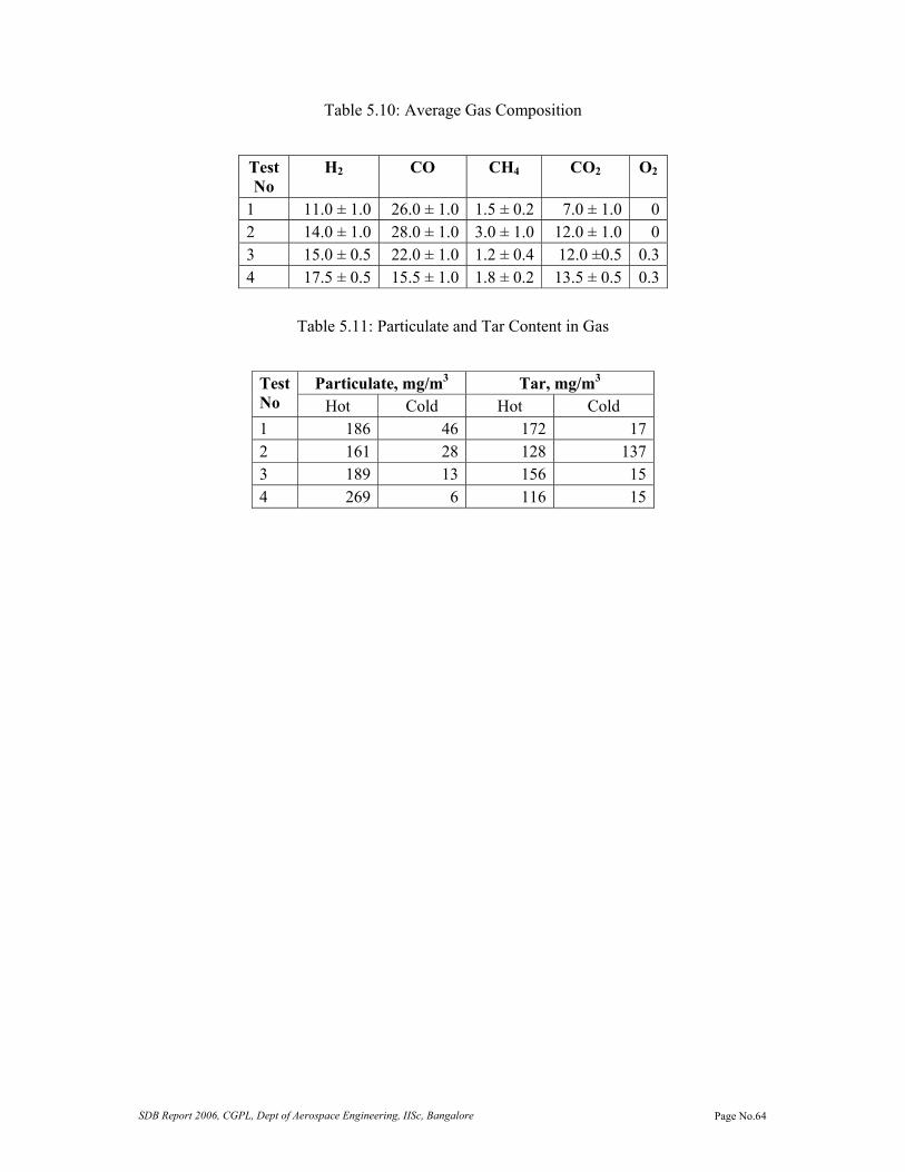
SDB Report 2006, CGPL, Dept of Aerospace Engineering, IISc, Bangalore Page No.64
Table 5.10: Average Gas Composition
Test No
H2 CO CH4 CO2 O2
1 11.0 ± 1.0 26.0 ± 1.0 1.5 ± 0.2 7.0 ± 1.0 0 2 14.0 ± 1.0 28.0 ± 1.0 3.0 ± 1.0 12.0 ± 1.0 0 3 15.0 ± 0.5 22.0 ± 1.0 1.2 ± 0.4 12.0 ±0.5 0.3 4 17.5 ± 0.5 15.5 ± 1.0 1.8 ± 0.2 13.5 ± 0.5 0.3
Table 5.11: Particulate and Tar Content in Gas
Test No
Particulate, mg/m3 Tar, mg/m3 Hot Cold Hot Cold
1 186 46 172 17 2 161 28 128 137 3 189 13 156 15 4 269 6 116 15

SDB Report 2006, CGPL, Dept of Aerospace Engineering, IISc, Bangalore Page No.65
(F2)
(SB
)
(FF
)
(FF
)(D
CC
)(DIE
SE
L P
UM
P)
(F2
)(F
2)
(F1
)
(C2)
(V1
)
(P1)
(V2
)
(V4
)
(V3)
(C2
)(C
2)
(WS
)
(R)
(N)
CO
AR
SE
FIL
TE
R
CE
RA
MIC
RE
AC
TO
R
FIN
E F
ILT
ER
IN D IR EC TC O O L ER
(E)
(PF
)
(GV
1)
(GV
2)
(V)
(P2)
LEG
ENDS
B1 :
BLO
WE
R 1
B2 :
BLO
WE
R 2
C1 :
BIO
MAS
S C
ON
VEY
OR
C2
: C
OO
LER
DC :
DIE
SEL
CAT
ALYT
IC C
ON
VER
TER
E :
D
IESE
L E
NGIN
ESF
:
FLAR
EF1
: C
OAR
SE F
ILTE
RF2
: F
INE
FILT
ERFF
: F
ABR
IC F
ILTE
RG
:
GR
ATE
GV1
/GV2
:GAS
VAL
VES
N :
N
OZZ
LES
O1
: OXY
GEN
SA
MPL
E 1
O2
: OXY
GEN
SA
MPL
E 2
PF :
PAP
ER F
ILTE
RR
:
REA
CTO
RSB
: S
UCTI
ON
BLO
WE
RV
: V
ENT
UR
IV1
TO
V4
: VA
LVES
WS
: WAT
ER S
EAL
(G)
1(C
1)
(W1)
(W2) W
AT
ER
RE
SE
RV
OIR
WA
TE
R T
O F
ILT
ER
WA
TE
R S
EA
LS
WA
TE
R T
O C
OO
LE
RS
W AT ER T O W AT ER SC R U B B ER
W AT ER T O A IR N O Z Z L E C O O L IN G
Figure 5.3: Schematic of 500 kg/hr gasifier at M/S Senapathy Whiteley, Ramanagara
SDB Report 2006, CGPL, Dept of Aerospace Engineering, IISc, Bangalore Page No.66
Thermal Gasifier at TANFAC TamilNadu Fertilizers and Allied Chemical (TANFAC) is a joint venture company between TIDCO and Aditya Birla group of companies. The management of TANFAC is by Aditya Birla group with TIDCO being sleeping partner. The main production at TANFAC is Aluminum Flouride (AlF3) which is used to meet the requirements of other companies of Birla group. One of the raw materials required in the production of AlF3 is hydrogen Flouride (HF). HF reactor needs heat at 600 0C for the process. This was met with by using 280 ltrs of HFO. With HFO cost rising, the production cost also increased and the end product cost was not competitive. The management decided to substitute HFO with producer gas and scouted for gasifiers to meet their requirement. After due deliberations, the order was placed to one of the IISc licencees, M/S Energreen Power ltd for 1100 kg/hr biomass gasifier. IISc team also studied the end use requirements and suggested a single reactor stream with elements akin to an electrical system. M/S TANFAC directly purchased Wesmann make dual fuel burner with air to fuel ratio controller. The system was built and erected in 8 months time and commissioned in July 2003. This was the first time with fixed bed downdraft, a single reactor of 1100 kg/hr tested. Initially the company found it difficult to source dry biomass daily to a tune of 25 tonnes. For around 8 months, the company operated the system for 450 kg/hr with mix of biomass and coconut shells depending on the availability. In this period, the company got equipped for handling the required amount of biomass and also built dryers for drying biomass utilizing waste heat from the gasifier and exhaust of the HF combustion chamber. After which the system was taken for higher power levels, the chiller which was down sized by the company for commercial benefits posed a limitation. The company took nearly a year after commissioning to overcome these limitations. Later when the system was tried for continuous operations to higher loads (around 700 kg/hr); carry over of charcoal into cyclone was observed. The charcoal carryover was on higher side to a tune of 150 – 200 kg almost blocking the cyclone. This not only interrupted the operation but also did not allow rated load operations. This phenomenon became repeatable at 700 kg/hr throughput after 6 – 8 hours of continuous operation. At this point of time, the reactor was unloaded and observed for clues, the observations were:
• The reactor face opposite to gas outlet had build-up of ash from below the nozzle to the bottom plate of the reactor.
• The grate location had been changed during fabricaton as against drawing. • The reactor had an additional reinforced sloping curve lining which restricted the gas
flow path. These were got corrected and subsequent runs showed occasional carry over but reactor pressure drop remained large and the rated throughput was difficult to be achieved and the frequent ash build up problem continued. Later trials also showed that char carryover was persistent at 750 kg/hr. The superficial velocity of gas at the bottom portion at this flow rate was found to be 1.2 m/s and hence it was decided to increase the bottom area to restrict the superficial velocity to around 0.65 m/s at rated flow rate which was prevailing in lower power level gasifier.

SDB Report 2006, CGPL, Dept of Aerospace Engineering, IISc, Bangalore Page No.67
Hence the bottom height of the reactor was increased by 800 mm. This solved the carryover problem but the rated output could not be consistently held. Several cold flow studies and transparent model reactor was operated to understand the phenomena. The model studies showed a preferential free bed movement with screw rotation resulting in one half portion (vertical) to remain stagnant. This was resulting in clinker formation and choking of the reactor and increased bed pressure drop with time. This also forced the reactor to be unloaded in every 500 hours of operation. Table 5.12 shows the amount of clinker formed in some of the operations
Table 5.12: Clinker formation details in early stages
Plant Run Bio mass used Clinker from reactor Biomass Feed tonnes after stoppage, kg Rate, kg/hr
02.7.04 - 10.7.04 84 670 500 - 600 30.7.04 - 07.8.04 104 1020 600 - 700 29.8.04 - 18.9.04 191 762 700 - 800
A second vertical grate was inserted from the bottom to arrest free flow of material. This helped in uniform material movement where in the entire cross section participates in gasification reaction. The rated biomass consumption was achieved and also the fossil fuel replacement. The final performance was even better than the guaranteed performance with saving of 280 lt/hr of FO at 3.5 – 3.6 kg/L which is 15% better leading to an approximate additional saving of Rs 4500 per day. A typical operational plot has been shown in Figure.5.4 and flue gas composition in Figure. 5.5. The flue gas analysis for the dual fuel burner in HF mode and dual fuel mode is shown in Table 5.13. The dual fuel operations have lower emissions as compared to HF operations. The system is presently operating at 2500 hours continuously with out any unloading. This plant has increased the learning and confidence in the technology.

SDB Report 2006, CGPL, Dept of Aerospace Engineering, IISc, Bangalore Page No.68
0
5
10
15
20
25
0 100 200 300 400 500
Time in mins
Gas
Com
posi
tion
%CO
H2
CO2
CH4
Figure 5.4: Typical Gas Composition at M/S TANFAC
0
100
200
300
400
500
600
700
800
900
1000
1 26 51 76 101 126 151 176 201 226 251 276
Time in Hours from start of the plant
Bio
mas
s co
nsum
ptio
n kg
/hr
IISc/EPL representatives present. Had noticed around 15 L/hr FO consumption
Figure 5.5: A typical operational plot at M/S TANFAC

SDB Report 2006, CGPL, Dept of Aerospace Engineering, IISc, Bangalore Page No.69
Table 5.13: Flue gas analysis details of HF burner
Date 14/06/2004 16/06/2004 17/06/2004 17/06/2004
Time 11:00 10:45 11:55 12:25
Analysis point: Pre Heter o/l to Chimney
Pre Heter o/l to Chimney
Pre Heter o/l to Chimney
Pre Heter o/l to Chimney
Plant load: 60 60 60 60
HF Burner chamber o/l temp:
560 560 554 554
Hot gas fan outlet: 390 390 405 405
Biomass plant load: 360 kg/hr of wood.
Not running. Not running. Not running.
Biomass Blower speed:
Not running. Not running. Not running. Not running.
Condition New 40HP blower for both Burner & drier
40HP (new) blower for drier & 20HP for Burner
20HP blower for burner and 40HP (old) for drier
20HP for burner alone.
CO/CO2 ratio: 0.0019 0.0025 0.0021 0.0016
CO in PPM: 86 185 165 138
CO2 IN %: 4.2 7.4 7.5 6.4
O2 in %: 15.3 11 10.8 12.3
SO2 in ppm: 0 436 634 482
Excess Air in %: 274 112 109 144
NO IN ppm: 29 107 113 70
NOx in ppm: 29 107 113 70
Temperature in 0C: 197 160 179.7 408.5
Ambient in 0C: 33.8 37 38.6 41.3
CAB Valve Opening to Burner: 70% 70% 70% 70%

SDB Report 2006, CGPL, Dept of Aerospace Engineering, IISc, Bangalore Page No.70
Part II

SDB Report 2006, CGPL, Dept of Aerospace Engineering, IISc, Bangalore Page No.71
Preface This part comprises of studies towards understanding of in-cylinder mechanism of a producer gas engines, myths related to optimum compression ratio for a producer gas engine and adaptation of commercially available natural gas engines. Though producer gas has been a fuel source for internal combustion engines during the times of petroleum source crunch, the subject has not been considered seriously by various researchers till recently. In fact past fifty years have seen enormous developments in the field of internal combustion engines for petroleum fuels with concentration on power to weight ratio and lowering of exhaust emissions. The IC engines community never considered producer gas as a fuel for engines largely due to non-availability of gasifier for commercial applications and success stories fuelling IC engines in western part of the world. Hence a need was felt that in the Strategic Development of Bio-Energy (SDB) project substantial effort to be put in understanding of producer gas engines and developments leading to commercial operations of producer gas engines. This has been accomplished and this first volume enumerates the efforts on development of producer gas engines. The work that is reported in here reemphasizes the potential of biomass-derived producer gas as an eco-friendly fuel. Experiments with low energy density producer gas in a high compression ratio (CR) spark ignition engine have shown the engine performance to be smooth without adverse effects of 'knock'. These experiments were conducted on a small power level spark-ignition engine (SPE) converted from a diesel engine at a CR of 17. The engine – alternator system was characterized for its performance by the simultaneous measurement of gas and airflow rates, gas composition (on-line), emission levels and power delivered. It was also instrumented to obtain the in-cylinder behavior in the form of pressure-crank angle (p - θ) diagram to assess the thermodynamic behavior of the engine. Experiments at varying CR (17 to 11.5) have established the benefits of operating the engine at higher CR in terms of lower de-rating and better efficiencies. These experiments also established the optimum parameters, namely the Minimum Advance for Brake Torque (MBT) and the corresponding equivalence ratio for maximum power. The findings from this study was further applied on a medium power level engine (MPE) of 200 kW and performed assessed. It was also found that the exhaust emission from the producer gas fuelled engines meet the emission norms of most of the countries. To understand the in-cylinder behavior, a zero-dimensional (thermodynamic) modeling has been conducted using wrinkled flame theory for flame propagation. The necessary inputs for this sub-model in terms of laminar burning velocity and turbulence parameters are obtained from discrete studies. The laminar burning velocity data at pressure and temperature typical of unburned mixture in engine is obtained from one-dimensional flame calculations. The turbulence parameters are obtained by conducting a 3-D CFD study on a bowl-in-piston geometry simulating motored or non-firing conditions. One experimental firing case is used as a test case in tuning the 0-D model in terms of constants required for computation of heat loss. Subsequently, keeping these parameters fixed 0-D predications are made for twelve test cases involving combustion chambers of SPE and MPE at varying CRs and ignition settings. These are further categorized under three sub-groups, namely Simple, Complex I and Complex II depending upon the intricacy involved in the predictions. Under the Simple sub-group, four test cases of SPE are dealt with, wherein the predictions match very well with the experimental p-θ curve. These computations are attempted assuming simple spherical flame propagation model. Whereas, under Complex-I sub-group, six cases of SPE are dealt, wherein the cylinder pressures are under-predicted with simple spherical flame propagation

SDB Report 2006, CGPL, Dept of Aerospace Engineering, IISc, Bangalore Page No.72
model. It is observed that in most of the cases, major part of the combustion occurs during the reverse squish period. A careful analysis of the motored CFD results indicated increased movement of the fluid out of the bowl during the reverse squish period. This fluid movement could modify the normal combustion process. The velocity vectors of the fluid indicate to a ‘Flat’ shape flame beyond the spherical flame engulfing the bowl. The change in the flame shape could enhance the effective burning area and thereby contribute to higher burn rate. These effects are termed, as ‘Reverse Squish Flame’ (RSF) hypothesis in this work and when these effects are accounted in the 0-D model the predictions are much better. Under Complex - II category, two test cases belonging to MPE are addressed. For these cases higher turbulence intensity is accounted due to higher mean speed of the piston (7.0 m/s) compared to SPE (5.8 m/s). Also additional flame kernel displacement is considered due to eccentric location of the ignition source. Even in these cases the predictions are better with RSF hypothesis. Also, work related to adaptation of commercial gas engines are reported here. There has collaborative work conducted along with Cummins India, wherein natural gas engines have been adapted for producer gas operation. This report contains details of the long duration tests conducted at the laboratory. As a consequence of successful testing, a large number of Cummins gas engines have been deployed in the field in the past two years for commercial operations. These details are also reported here.

SDB Report 2006, CGPL, Dept of Aerospace Engineering, IISc, Bangalore Page No.73
Chapter I Introduction and Literature Review In the recent times, gaseous fuels are gaining prominence as cleaner fuels for power generation via internal combustion engine route, the power generation package including both reciprocating engines and gas turbine machinery. Complete combustion with minimal emission is the key feature of gaseous fuels and this feature is currently being exploited the world-over for power generation purposes. Producer gas derived from biomass is one such eco-friendly gaseous fuel. While natural gas is the most used one, next one being the land fill gas or biogas, which is diluted natural gas (with 20-30% CO2) biomass based producer gas is perhaps the least used fuel, hence the literature in the area is scant. The literature review is categorized into three sub-topics, namely producer gas engines addressing the experimental part, fluid flow in reciprocating engines and combustion studies in spark ignition engines the modeling aspect. Introduction Internal combustion reciprocating engines have integrated into societal service in the last century. Their use has improved the quality of life substantially, but at the cost of degradation to the environment, certainly in several countries with insufficient environmental consciousness. Therefore, large impetus is being given to improve the efficiency and thereby reduce the emissions by using two approaches namely, improvement in engine design and use of alternate fuels in place of fossil fuels. In the domain of engine design, the complex fluid dynamics and thermo-chemical interaction occurring in the combustion chamber play an important role in the eventual efficiency and emissions released. One way to reduce the emissions is to adopt leaner combustion for which understanding fluid dynamics inside the combustion chamber becomes pertinent. Many tools in the form of computational modelling have been used both in the past and the present to understand these phenomena in zero dimensional phenomenological modelling to full-fledged three-dimensional modelling. In the domain of alternate fuels, oxygenated liquid and gaseous fuels receive more prominence because of the possibilities of cleaner combustion. Among the gaseous fuels, producer gas, a low-energy density gas derived from biomass holds a large promise as an environment friendly fuel. This fuel gas in addition to being CO2 neutral generates lesser quantum of undesirable emissions. Even though these merits of biomass have been recognized widely, the technological capitalization has remained in infancy largely. The thermo-chemical conversion of biomass leads to a gas generally termed as producer gas. The process is termed gasification implying that a solid fuel is converted to a gaseous fuel. Gasification is not a new technology but is known ever since World War II. During this period a number of vehicles in Europe were powered with charcoal gasifiers. It is estimated that over seven million vehicles in Europe, Australia, South America and Pacific Islands were converted to run on producer gas during World War II. These engines were spark ignition (SI) engines, mostly in the lower compression ratio (CR) bracket operating either on charcoal or biomass derived gas. It is appropriate to mention here the contribution of National Swedish Testing Institute of Agricultural Machinery, Sweden whose extensive fieldwork conducted by

SDB Report 2006, CGPL, Dept of Aerospace Engineering, IISc, Bangalore Page No.74
mounting gas generator and engine set on truck and tractors has provided an important demonstration of the enormous possibilities. In the recent times, there is a renewed interest in biomass gasification technology, which has stimulated interest in producer gas operated engines. Whatever work has been attempted in this area has been limited to lower CR (less than 12.0) engine due to perceived limitation of knock at higher CR. A review of some of earlier studies relevant to this work, namely producer gas engine, fluid flow in reciprocating engines and combustion studies in SI engines are presented now. Literature Review Producer Gas Engine Literature survey in the field of producer gas based engines reveals modest research work accomplished since the inception of biomass/charcoal gasification systems. This could be attributed to two reasons, namely non-availability of standard gasification system that could generate consistent quality producer gas and the other relating to misconceptions about producer gas fuel. These issues are addressed in Chapter II, which contains the description of biomass gasification process along with application of producer gas in reciprocating engines. The literature survey on this particular topic addresses some of research activities conducted in Europe, America and the Indian sub-continent. It is reported that Europe exploited the most of gasification technology during petroleum oil crisis of World War II. Among the European nations, Sweden accounts for a large amount of work in the area of wood and charcoal gasification. National Swedish Testing Institute of Agricultural Machinery, Sweden [ANON-FAO Report, 1986] has reported extensive work on the design and development of closed top charcoal and wood gasifiers for use with the reciprocating engines. These reciprocating engines were mostly diesel engines mounted on trucks and tractors for operation in dual-fuel mode. Many finer aspects relating to dual-fuel operation have been extensively reported, with cumulative operational experience exceeding a few thousand hours. However, whatever work was conducted on the producer gas alone operation is either proprietary to the engine manufacturers or is not adequately reported in the public domain literature. These engines were however in the lower CR – 10 either adapted from petrol engines or modified diesel engine. In the recent times, Martin et al [1981] have reported work using charcoal gas and biomass based producer gas on a SI engine with a de-rating of 50% and 40% respectively at a CR of 7. However, the same authors claim 20% de-rating when worked with producer gas at a CR of 11. They indicate an upper limit of CR of 14 and 11 for charcoal and biomass based producer gas respectively. However, there is no presentation of experimental evidence in favour of these results American sub-continent also claims experimental work relating to producer gas engines. Tatom et al [1976] have reported working on a gasoline truck engine with a simulated pyrolysis gas at a de-rating of 60-65%. The authors have also identified the optimum ignition timings as a function of speed. Parke et al [1981] have worked on both naturally aspirated and super charged gas engines. The authors claim a de-rating of 34%, compared to gasoline operation and a lesser de-rating in a supercharged mode. The authors discuss aspects relating to fuel-air mixture ratio, flame speed and its relation to the ignition timing for producer gas operation. They have also identified the best possible mixture for maximum power and efficiency along with ignition timing at various speeds.
SDB Report 2006, CGPL, Dept of Aerospace Engineering, IISc, Bangalore Page No.75
In the Indian sub-continent, work in the area of producer gas engine has been reported by the biomass gasification group of Indian Institute of Technology, Mumbai. Shashikantha et al [1993, 1999] and Parikh et al [1995] have reported work on a gas engine converted from a naturally aspirated diesel engine at CR of 11.5. The reason for limiting the CR is cited to be the knocking tendency; however, no experimental evidence is provided in support of it. The work is reported on a gas engine converted from a diesel engine with a modified combustion chamber. The modified combustion chamber of Hesselman (shallow W) shape is claimed to enhance the in-cylinder turbulence by suppression of swirl and promotion of squish effect. With the above modification, a power output of 16 kW is reported in gas mode against a rated output of 17 kW in diesel mode. The maximum thermal efficiency is claimed at 32%, which is close to the results in compression ignition (with diesel) mode at an output of 15 kW. It is quite surprising to note the conversion efficiencies to be same, when the CRs are widely different. The authors also claim an optimum ignition timing of 35° BTC compared to 22° BTC for natural gas on the same engine. With the producer gas claiming to contain about 24.1% H2, 21.5% CO and 2.1% CH4 the burning velocities ought to be higher than natural gas. In contradiction to the reported ignition timing, the claimed gas composition would require the ignition timing to be located close to TC. Therefore, it is not clear as to how such a large output was obtained at advanced ignition timing when all logics point towards retarded ignition timing (as also demonstrated in this work). The only earlier experimental work in the higher CR range is reported by Ramachandra [1993] on a single cylinder diesel engine (CR=16.5) coupled to a water pump. A power de-rating of 20% was reported at an overall efficiency of 19% without any signs of detonation. This work does not report of detailed measurements like the gas composition, pressure-crank angle diagram and emissions, which are essential for systematic investigation and scientific understanding. If one were to summarize the findings of earlier studies, it becomes evident that no systematic investigation has been attempted so far in identifying if limitation of knock exists with producer gas operation at CR comparable with the diesel engine operation. This topic is worth analyzing since producer gas contains a large fraction of inert (> 50%) and with laminar burning velocity being high (due to the presence of H2), smooth operation at higher CR does not seem impossible. These aspects are very vital in establishing the fact that close to comparable power (with a lesser extent of de-rating ~ 15-20%) could be achieved with producer gas by operating in engines at higher CR. Fluid Flow in Reciprocating Engines Fluid dynamics inside the engine combustion chamber plays a predominant role in the operation of an internal combustion engine. Fluid flow governs mixing, combustion and heat transfer processes in reciprocating engines. The in-cylinder swirl and turbulence affect the burn rate depending upon the combustion chamber design and intake port configuration. Studies have established in-cylinder flow to be extremely complex and three-dimensional in nature. Due to their highly turbulent nature, the in-cylinder flows are not easily quantified. But to improve the combustion process and thereby economy and emission, a better understanding of the relationship between the in-cylinder flow field and combustion process becomes necessary. In an attempt to do this, a number of experimental studies have been conducted including the flow visualization by researchers like Ekchian et al [1979], Hirotomi et al [1981] and Namazian et al [1980]. Similarly, researchers like Acroumanis et al [1987]

SDB Report 2006, CGPL, Dept of Aerospace Engineering, IISc, Bangalore Page No.76
and Bicen et al [1985] have studied flow past valves of different configurations and their effect on the subsequent in-cylinder flow field. All these aspects have been subsequently brought out in the review paper by Acrounamis et al [1987]. The emergence of various laser anemometry techniques over the last few decades has given researchers a non-intrusive method of measuring velocities in combustion chamber. Amongst the large number of workers Fanslar [1985], Ikegami et al [1987], Corcione et al [1994], Floch et al [1995], Yoo et al [1995] and Catania et al [1996], Einewall et al [1997]. Corcione et al [1994] have studied the in-cylinder turbulent flow field in a modern diesel engine – with a re-entrant geometry, motored over a wide range of speeds (1000 to 3000 rev/min). They highlight the jet character of the intake flow that generates large-scale rotating flow structures during intake and compression process. The large-scale rotating structure is observed to be highly turbulent and unstable, and is indicated to achieve greater stability during the compression process. In case of the re-entrant geometry, the authors observe that turbulence intensity tends to increase in the early stages of the expansion process, unlike the falling trend with the conventional cylindrical geometry. This increase in turbulence intensity is attributed to higher shear zones with re-entrant geometries. Similar behaviour has been observed by Catania et al [1996], who has measured turbulence quantities using hot wire anemometer in combustion chamber of an automotive diesel engine with a slightly re-entrant geometry at varying speeds from 600 to 3000 rev/min. The variation of turbulence intensity with time as a function of engine speed is clearly brought out. In another work, Einewall et al [1997] have studied six combustion chambers namely, Nebula, Turbine, Re-entrant square and Re-entrant cylindrical, Quartette and Fair top in a supercharged natural gas engine. Results pertaining to turbulence intensity and burn rate for each of the combustion chamber are discussed. Quartette chamber is reported to have a favourable turbulence intensity peak, with a positive influence on the performance in terms of higher efficiency and lower emissions with lean mixtures. In parallel with the experimentation, a detailed modelling of engine flow processes has become a new-found tool in generating a wealth of information. A number of researchers, namely Schapertons et al [1986], Wakisaka et al [1986], Jennings [1992], Trigui et al [1994], Han et al [1995], Bauer et al [1996], Jones et al [1995], and Lebrere et al [1996], have worked on 3-D computational studies with respect to the fluid flow in engine cylinder, simulating the motored or non-fired condition. CFD studies focusing on engine related work, address either the complete flow, encompassing the manifold and the engine cylinder or in part. Majority of the studies addresses geometries formed by a moving piston either flat or bowl and without or with moving intake valve. For cases not involving the intake valve, the initial condition for the compression process is taken as spatially uniform based either on empirical correlations or on single point experimental measurements. In the case of geometry with moving valve, suitable boundary condition is considered upstream of the intake valve or manifold. The Study by Schapertons et al [1986] on bowl-in piston geometry reveals higher turbulence levels compared to the flat piston geometry due to enhanced swirl and squish effect. This study has been conducted on eccentric, reentrant bowls using standard k-ε model. The prediction depicts strong radial inward squish flow at the lip of the bowl near Top Centre (TC). The bowl-axis offset also seems to produce complex flow field in the bowl resulting in substantial spatial variation in turbulence intensity within the bowl. Trigui et al [1994] have

SDB Report 2006, CGPL, Dept of Aerospace Engineering, IISc, Bangalore Page No.77
checked the feasibility of using experimentally determined flow field at the intake valve closure as the initial condition for the compression process. The authors observe the study to be feasible, and that with adequate vector field data from the 3-D Particle Image Velocimetry (PIV) as the initial condition the overall error in prediction of subsequent flow field is modest. Han et al [1995] have proposed a high Reynolds-number RNG k-ε model for variable-density flows by including the effects of velocity dilatation and kinematics viscosity variation in the turbulence dissipation rate. Computations have been made of compressing/expanding flows in a production diesel engine consisting of a piston with bowl arrangement. The computation does not account for intake flow and therefore a uniform initial condition is assumed at the beginning of computation. The predicted trend of increasing turbulence intensity due to squish late in the compression process and the magnitude of the integral length scale near TC seems to compare well with that of single point PIV measurements. The ability of k-ε model in predicting turbulence quantities under engine like conditions has been examined by Lebrere et al [1996] by comparing with higher order Reynolds stress model on simple flat piston geometry. The Reynolds stress model predicts the presence of anisotropy during compression and it is attributed to be the reason for higher u’ values with k-ε mode1 (~ 20% higher). Summarizing findings from the above studies, the predictions using simpler turbulence models (k-ε model) seem to compare well with the available experimental results. Therefore using CFD to generate necessary flow field data for further modelling seems to be feasible.
Combustion Studies in Spark-Ignition Engine
Figure. 1.1 Engine Flame Regime Shown on Da vs. TRe Plot, From Abraham et al [1985]
Combustion in a SI engine has been observed to be turbulent in nature, governed by the physical and chemical processes and the complex interaction between them. Turbulent

SDB Report 2006, CGPL, Dept of Aerospace Engineering, IISc, Bangalore Page No.78
premixed combustion is essentially characterized by dimensionless parameters, namely turbulent Reynolds number (ReT), a ratio of turbulence inertial to viscous force and Damkohler number (Da), a ratio of characteristic flow time to characteristic chemical time. The other parameter of interest is the ratio of Kolmogorov length scale lk to laminar flame thickness δL, which provides a measure of distortion of a laminar flame front by the turbulent flow. Turbulent flames are primarily classified into two regimes; namely, the wrinkled flame and the distributed reaction zone, the above-mentioned parameters identify the regime of a flame. Many researchers have addressed the question of identifying the regime of engine flames. These studies have indicated the value of Da and ReT for a typical SI engine to lie in the wrinkled flame regime as shown in Figure 1.1 - identifying the engine flame among different turbulent flame regimes [Abraham et al, 1985]. A sufficient condition for the wrinkled flame regime is lk >> δL. Abraham et al [1985] has observed the ratio of lk/δL to be more than unity based on engines of different configurations. In this case, one definition for laminar flame thickness is the ratio of thermal diffusivity in the reactants to the laminar burning velocity Abraham et al [1985]. The fact that engine flame is wrinkled [Keck, 1982; Heywood 1988] has been established based on experimental evidence, largely from Schlieren photographs and studies of flame structure using laser diagnostics. It is observed that early in the burning process the flame is a thin, moderately wrinkled but simply connected front or reaction sheet between unburned and burned gas. The thickness is reported to be about 0.1 mm, which is comparable to the thickness of a laminar flame under the prevailing engine conditions. The scale of wrinkles is about 2 mm at engine speeds of 1000 to 2000 rev/min. As the flame propagates across the chamber, the flame front is observed to become more convoluted, with the scale of wrinkles tending to decrease with time. Further evidence that a thin reaction sheet front becomes highly wrinkled and convoluted by the turbulent flow field into a thick turbulent flame “brush” is provided from the Schlieren studies conducted by Heywood et al [1984]. Experiments with propane–air mixture and hydrogen-air mixture indicate a turbulent flame thickness of 4 to 5 mm and 1.5 mm respectively. The lower flame thickness with hydrogen-air mixture is attributed its higher laminar burning velocity, whereby the increase in Da shifts the flame toward the wrinkled flame regime. Similar wrinkled structure has been observed by Namazian et al [1980] and Gatowski et al [1984] using Schlieren photography. The laser shadowgraphs acquired by Witze [1982] effectively captures the effect of spark location on the turbulent flame structure.
Figure. 1.2: Concept of Wrinked/Flamelet Regime in the Premixed Turbulent Flame.

SDB Report 2006, CGPL, Dept of Aerospace Engineering, IISc, Bangalore Page No.79
Laser scattering experiments conducted by Smith [1982] reveal similar such wrinkled structure with the flame becoming increasingly finely wrinkled due to increase in engine speed on account of enhanced turbulence intensity and reduction in turbulence scale. The concept of wrinkled flame is shown in Figure 1.2. A thin laminar flame front of thickness (δL) is seen propagating into the unburned mixture, which is highly turbulent. The flame becomes increasingly distorted by the turbulent flow field through which it is propagating and develops a highly wrinkled and probably multiply-connected structure as shown to the left in Figure. 1.2, where δT is the thickness of the flame brush. The above stated experimental evidence indicates that the developed turbulent flames in SI engines, under normal operating conditions are highly wrinkled and probably multiply connected thin reaction sheets [Keck, 1982; see Heywood 1988]. The overall thickness of the turbulence flame brush is reported to be of the order 10 mm, with the reaction sheet thickness being 0.1 mm. The scale of wrinkles is reported to be 1 mm. This, therefore, establishes the engine flame to lie above lk/δL=1 line, within the wrinkled flame or flamelet combustion regime. Modelling of engine cyclic processes has been addressed extensively covering a wide range of fuels including liquid and gaseous fuels. In the area of gaseous fuels, propane and natural gas have received sufficient attention including multi-dimensional combustion modelling. The ability to utilize experimental data in new situations and conditions other than those where experiments are conducted is truly enhanced by using mathematical modelling. Mathematical modelling involves a combination of appropriate assumptions and equations describing a process under consideration and thereby allows critical features of a process to be analyzed. Modelling is being seriously pursued to acquire physical insight of the critical processes and thereof suggest suitable improvements based on the derived understanding. These are expected to become more robust with improvements in physical understanding over a period of time. Mathematical modeling calibrated with experimental data can provide a powerful predictive tool to decide on new designs as well make good predictions for new and complex situations. Modelling is classified as thermodynamic or fluid dynamic based on the equations that provide the model its predominant structure are either based on energy conversation or on a complete analysis of fluid flow [Heywood, 1988]. The thermodynamic models are more popularly known as zero-dimensional (0-D), phenomenological or quasi-dimensional models. The fluid-dynamic based models are often multidimensional due to their inherent ability to provide detailed information of the flow field and these involve solving of governing conservation equations. In the recent times, detailed 3-D modelling of engine combustion using Computational Fluid Dynamics (CFD) has been investigated by Jennings [1992], Khalighi et al [1995] and Watkins et al [1996]. Jennings has simulated combustion using a fully turbulent combustion process, represented essentially as a two-zone model as represented in 0-D combustion models. However, unlike what has been observed experimentally in engine flames, the combustion is assumed to occur at multiple burning sites within the flame front. Khalighi et al [1995] have worked on flow visualization studies and simulations using flamelet combustion model on a four-valve-per cylinder SI engine. The authors have addressed issues relating to the application of CFD to engine modelling, which includes that of numerical inaccuracies. The authors discuss the technique adopted for near-wall combustion and the merits of flamelet model vis-à-vis the Arrhenius and turbulence-mixing-controlled model in predicting the mass burn. The authors also identify a mesh density of 1 million grid points for

SDB Report 2006, CGPL, Dept of Aerospace Engineering, IISc, Bangalore Page No.80
obtaining grid-independent solution for cold flows, with errors estimated at 10 to 15% at lower mesh densities. Watkins et al [1996] have simulated combustion and turbulence using flamelet and second order-moment closure models respectively. The authors claim turbulence anisotropy to be better represented by the second order-closure approach. Also the superiority of flamelet model as compared to eddy-burn-up model in predicting burn rate along the wall has been demonstrated. Similarly, simpler models like the 0-D modelling have been addressed by a number of researchers due to their advantage that they could be put to immediate use till better understanding prevails in the complex-turbulent combustion process. The phenomenological models are structured from the first law of thermodynamics formalism in which the only real independent variable is crank angle or time. Different approaches are used in modelling some of the important processes or phenomena occurring in the complex thermo-fluid dynamic environment in the engine cylinder. The in-cylinder phenomenon modelled could be either burn rate, boundary layer heat transfer or pollutant formation depending upon the focus of the study. Since ‘burn rate’ phenomenon is of interest in this work, it has been dealt with in the following paragraphs. The burn rate in reciprocating SI engine is specified by some functional relationship where the start of combustion and combustion duration are related to the crank angle. Two examples of such functions are the Cosine burning law and Wiebe function [see Heywood, 1988]. The burn rate modelling is deficient because there is no physics involved in such an approach. In an attempt to alleviate such inadequacy, several researchers have proposed models to predict the burn rate in SI engines. Such models are based on fundamental quantities such as turbulence intensity and the turbulence length scales with specified kinetics. These models are required to predict the burn rate for a wide range of operation conditions like spark timing, equivalence ratio and engine speed. Burn rate is often expressed as:
Tfub SA
dtdm
ρ= (1.1)
Where ρu is the unburned gas density, Af is the flame front area and ST the turbulent flame speed or the burning velocity. Mechanistically ST has been related to laminar burning velocity, SL by the expression known as the Flame Speed Ratio (FSR), which is the ratio of ST to SL. There are a number of correlations available for calculation of FSR. Lancaster et al [1976] correlated the FSR with the turbulence intensity. A diagnostic combustion model, based on the assumption that flame propagates from the spark plug as a sphere, was used to determine burning velocities from the cylinder pressure-time data measured on a Cooperative Fuels Research (CFR) engine operating with propane. Similar correlation exhibiting FSR as a linear function of u’/SL emerged from the studies of Mattavi et al [1978], Abel-Gayed et al [1976] and Ballal et al [1974]. Most of these correlations assume the following form
LS
uCCFSR'
21 += (1.2)
Where C1 and C2 are constants. In one such work by Groff [1987] on a constant volume vessel the value of C1 and C2 are found to be 2.273 and 1.681 respectively. Another approach to model the turbulent flame propagation is entrainment and subsequent laminar burn-up of discrete, coherent, turbulent eddies; Blizard and Keck [1974, 1982] used

SDB Report 2006, CGPL, Dept of Aerospace Engineering, IISc, Bangalore Page No.81
this concept to calculate the burn rate in SI engines. This model has been formulated based on a series of experimental investigations that include Schlieren photographs, Shadowgraph and laser scattering measurements. The model postulates a wrinkled turbulent flame formed by the distortion of a thin reaction sheet (δL) due to surrounding turbulent flow field. The flame propagation is modelled as a two-zone model, where the wrinkled multi-connected laminar flame separates the burned and the unburned mixture. They assumed that the entrainment front moves with respect to the unburned mixture at a constant velocity uT that is proportional to turbulence intensity. Upon entrainment, each eddy burns in a characteristic time τb, which depends on the eddy size l T and laminar burning velocity SL. This model can be summarized by the following two equations.
bLfu
b SAdt
dmτμ
ρ += (1.3)
bTfu uA
dtd
τμρμ
+= (1.4)
where )( fTu AA −= llρμ . Al and Af are laminar and spherical flame area respectively. Equation 1.3 represents the mass burn rate; Equation 1.4 represents the rate of change of unburned mixture within the flame front. For the two quantities namely the characteristic speed, uT and characteristic length, l T in equations 1.3 and 1.4, Keck [1982] has provided an empirical relationship by coupling with a few variables relating to engine of simple geometry. The author concludes that the burning equations for complicated engine geometry with squish and swirl needs further examination. This model is discussed in detail in section 4.1.2 of Chapter IV. Tabaczynski et al [1977] worked on the eddy entrainment concept and postulated the following theory. The vorticity in the turbulent flow field is concentrated in vortex sheets that are of a size comparable to Kolmogorov scale lk. These vortex sheets are assumed to have a characteristic spacing that is of the order of the Taylor micro scale lM related to integral length scale lI and turbulent Reynolds number ReT. Based on these assumptions it is argued that ignition sites propagate along the vortex sheets with a velocity u’+SL, where u’ is the local turbulence intensity. The propagation of the reaction front between the vortex sheets is assumed to be laminar. In the recent work reported by James [1990] on an engine with flat piston geometry, the author has compared the experimental pressure-time data with the 0-D results. The predictions are made with an assumption of ‘thin’ and ‘elliptical’ turbulent flame instead of the ‘thick’ and ‘spherical’ flame up to a certain point, beyond which a thick and spherical flame is assumed. The point of transition is related to increased heat loss on account of higher surface-to-volume ratio at the time of completion of combustion. The author observes that thick turbulent flame could well be valid for the complete flame propagation, with flame shape tending towards ellipsoid at higher CR from that of spherical at lower CR. If one were to summarize the findings of the above studies, the entrainment and laminar burn-up model seems to be an established model for predicting burn rate provided parameters related to turbulence are properly accounted for a given engine geometry. However, there are open questions concerning the uniformity of the turbulence flow field for complex geometries involving swirl or squish, spherical flame assumption and flame movement subsequent to

SDB Report 2006, CGPL, Dept of Aerospace Engineering, IISc, Bangalore Page No.82
kernel formation. Detailed modelling of the fluid dynamics needs to be pursued to assess the validity of the model. Approach of the Present Work Based on the review of the earlier work, it is clear that there is no positive evidence for the presence of knock with producer gas fuel in spark ignition (SI) engines at high CR. This restriction in CR appears to be simply a matter of presumption rather than fact. Therefore, one of the primary objectives of this work is to attempt to operate a SI engine at the highest possible CR and establish the performance of the engine. This has called for a systematic investigation where all parameters relevant to engine characterization, namely gas and airflow rates, gas composition (on-line), emission levels and power delivered are recorded simultaneously. For combustion diagnosis, the cylinder pressure history data is also acquired and it later provides a basis to assess the thermodynamic behaviour of the engine. The producer gas fuel is generated from the well-established open top re-burn down draft gasifier system using Casuarina wood pieces as fuel. It is evident from the literature that in-cylinder processes in a reciprocating engine are extremely complex in nature. While much is known about these processes, they are not adequately understood at a fundamental level. Therefore at present, constructing a model to predict the engine operation from the governing equations alone is difficult. Nevertheless, simpler models like the 0-D are helpful in analyzing the thermodynamic behaviour and identifying key parameters responsible for such behaviour. One such approach based on the above lines has been adopted in this work. The objective of the current modeling effort is to simulate the burn rate in a producer gas fuelled SI engine under the influence of varying ignition timing and CRs. Therefore, heat release forms the critical part of the model, with simpler gas exchange model to complete the thermodynamic cycle. Eddy entrainment and laminar burn-up (EELB) postulated by Keck is adopted to compute burn rate with parameters of turbulence properly accounted for engine geometry under study. This called for a detailed three-dimensional CFD modelling of the actual engine geometry to obtain relevant parameters of turbulence under non-firing conditions. The data on laminar burning velocity have also been generated at pressures and temperature relevant to engine operation. Using these data, the cylinder pressure-time histories are predicted for two combustion chamber geometries at various CR and ignition timings. The limitations of the EELB model have been examined. Summary From the literature survey in the field of producer gas engine it clear that no attempt has been made to understand whether knock occurs with producer gas operation. The existence of knock appears more of a presumption. In the field of modelling of SI engines, Eddy Entrainment and Laminar Burn-up model proposed by Keck [1982] appears to be validated model to be used as a predictive tool for simple geometries. In order to implement the model on complex geometries (piston with bowl) requires apriori information on the turbulence level in the geometry. This could be quantified by experiments or through further computations. Use of CFD for computation of turbulence parameters appears to be rational based on the validation of the results with turbulence models such as ε−k in most cases.
SDB Report 2006, CGPL, Dept of Aerospace Engineering, IISc, Bangalore Page No.83
Chapter II Producer gas Properties This chapter provides properties of producer gas derived from biomass. Technological aspects relating to clean and consistent quality gas generation are discussed along with a few results related to gasifier performance in the part I of the report. Properties of Producer Gas Some of the fundamental data relating to producer gas are compared with pure gases in Table - 2.1. The comparison of producer gas with methane is more vital with regard to the internal combustion engine operation. This is because most of the engines operating on gaseous fuels are either close to pure methane (natural gas) or diluted methane (bio-gas, land-fill gas). The fuel-air equivalence ratio (actual fuel to air ratio)/(stoichiometric fuel to air ratio) at the flammability limits [Kanitkar et al, 1993] compares closely for both the gases, but the laminar burning velocity for producer gas at the lean limits is much higher. The laminar burning velocity for producer gas (at 0.1MPa, 300K) is about 0.5 m/sec [Kanitkar et al, 1993], which is about 30% higher than methane. This feature is argued to demand lower advancement in the ignition timing and needs consideration while arriving at the optimum ignition timing for the producer gas fuel. Like any other gaseous fuel, producer gas can be used for internal combustion engine operation provided the gas is sufficiently clean such that contaminant does not accumulate in the intermediary passages to the engine cylinder. But this fuel has largely been left unexploited due to additional perceptions, namely (1) auto-ignition tendency at higher CR, (2) large de-rating in power due to energy density being low. However, these perceptions need re-examination and clarification. The arguments against the classical view in favour of better knock resistivity are as follows. Firstly, with the laminar burning velocity being high due to the presence of hydrogen (more so, with the gasifier system adapted in this work) might reduce the tendency for the knock. Secondly, the presence of inert in the raw gas (CO2 and N2) might suppress the pre-flame reactions that are responsible for knocking on account of increased dilution. Also the maximum flame temperature attainable with the producer gas being lower compared to conventional fuels like methane, one could expect better knock resistivity. An examination of literature shows that producer gas has not been subjected to study on knock behaviour. Further, there is a general perception that producer gas being a low-density energy fuel, the extent of de-rating in power would be large when compared to high- energy density fuels like natural gas and Liquefied petroleum gas. This could be misleading because what needs to be accounted for comparison is the mixture energy density [Fleischer et al, 1981] and not the fuel energy density per se. On comparison with CH4, the mixture energy density for producer gas is lower by 23% as reflected in Table 2.1. The product to reactant mole ratio for producer gas is less than one. These two parameters could contribute to de-rating of engine output. However, it might be possible to reduce de-rating by working with engines of higher CR, perhaps higher than what has been examined using natural gas (CR=15.8) by Das et al [1997].
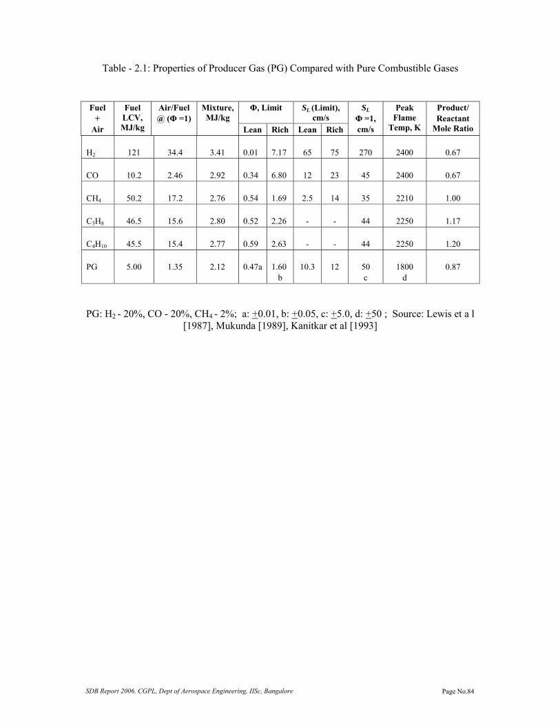
SDB Report 2006, CGPL, Dept of Aerospace Engineering, IISc, Bangalore Page No.84
Table - 2.1: Properties of Producer Gas (PG) Compared with Pure Combustible Gases
Fuel
+ Air
Fuel LCV, MJ/kg
Air/Fuel @ (Φ =1)
Mixture, MJ/kg
Φ, Limit SL (Limit), cm/s
SL Φ =1, cm/s
Peak Flame
Temp, K
Product/ Reactant
Mole Ratio Lean Rich Lean Rich H2
121
34.4
3.41
0.01
7.17
65
75
270
2400
0.67
CO
10.2
2.46
2.92
0.34
6.80
12
23
45
2400
0.67
CH4
50.2
17.2
2.76
0.54
1.69
2.5
14
35
2210
1.00
C3H8
46.5
15.6
2.80
0.52
2.26
-
-
44
2250
1.17
C4H10
45.5
15.4
2.77
0.59
2.63
-
-
44
2250
1.20
PG
5.00
1.35
2.12
0.47a
1.60
b
10.3
12
50 c
1800
d
0.87
PG: H2 - 20%, CO - 20%, CH4 - 2%; a: +0.01, b: +0.05, c: +5.0, d: +50 ; Source: Lewis et a l [1987], Mukunda [1989], Kanitkar et al [1993]

SDB Report 2006, CGPL, Dept of Aerospace Engineering, IISc, Bangalore Page No.85
Chapter III The Experimental Work This chapter discusses the experimental work conducted on spark-ignited gas engines fuelled with biomass-derived producer gas. The experimental work is presented in two parts. The first part discusses experiments on a Small Power level Engine (SPE), converted from a diesel engine and tested at varying compression ratio. The second part deals with experiments on a Medium Power level Engine (MPE) at a fixed compression ratio of 12. The results of performance are compared with baseline results obtained with diesel fuel in compression ignition mode of operation. Introduction This experimental work is considered in the background of the weak information base on producer gas engines in the literature. However, with the perceptions of the author being different from that quoted in the literature relating to operations at high compression ratio (CR), a thorough scientific investigation was launched for the first time. The primary investigation is conducted on an engine of 24 kW nominal capacity. For this purpose, a commercially available production diesel engine of CR = 17 is chosen for conversion to a spark-ignition (SI) engine. The engine operations have been found to be challenging with respect to data acquisition of engine cylinder pressure history due to severe electro-magnetic interference from the mechanical ignition system, which seriously hampered the working of the computer, a part of the data acquisition system in the initial stages. This was resolved subsequently through electrical circuit changes. Small Power level Experiments Description of the Engine Small power level engine (SPE) experiments were conducted on a spark ignition (SI) engine converted from a naturally aspirated, three-cylinder, direct injection diesel engine (RB 33 model) of compression ratio (CR) 17. The reason for choosing this particular CR diesel engine is explained as follows. It is known from fundamental thermodynamics that it is beneficial to operate an internal combustion engine at as high a CR as possible in order to attain high overall efficiencies. But the gain in efficiency beyond a certain CR can be expected to be marginal due to the other counter influencing factors such as increased heat loss and friction. But in the case of a SI engine the limitation of CR comes from a supplementary factor namely, ‘knock’. It is to be noted that knock sensitivity identifies the Highest Useful Compression Ratio (HUCR) for most of the fuels. However, for higher-octane fuels, it has been experimentally established that the upper limit of CR is 17 beyond which there is a fall in efficiency [Caris et al, 1959]. The inference drawn by Caris et al [1959] is based on extensive tests conducted on a multi-cylinder engine at varying CRs up to 20, using iso-octane doped with anti-knock agent. The variation of thermal efficiency with CR from the work of Caris et al

SDB Report 2006, CGPL, Dept of Aerospace Engineering, IISc, Bangalore Page No.86
Compression Ratio
The
rmal
Eff
icie
ncy,
%
Figure 3.1: Full Throttle Thermal Efficiency in SI Engine - 2000 rev/min, From - Caris et al [1959].
[1959] is shown in Figure. 3.1. The decline in efficiency beyond CR of 17.0 is attributed to delayed or late burning leading to increased heat loss. If one were to consider this as the upper limit and since no other work has been reported at higher CR for SI engines, choosing a production engine in CR = 17 for the current study appeared to be meaningful.
The salient features of the diesel engine chosen for conversion to SI engine are shown in Table 3.1. The naturally aspirated engine of 3.3 Litre capacity is designed at a CR =17, to operate at an air-to-fuel ratio of 20 - 21 (with diesel) at a rated conditions. The engine employs an in-line fuel injection system along with multi-hole injectors to atomize diesel at a pressure of 180 bar. The air intake system is comprised of an air filter, manifold and runner to each cylinder head. The intake port is of a simple design – directed type with air entering into the cylinder all around its periphery. The engine is designed with a valve overlap of 64° CA (refer Figure. 6.2 Chapter VI). The combustion chamber of the engine is formed of a flat cylinder head and slightly offset bowl-in piston as shown in Plate 3.1 and in Figure. 7.1 of Chapter VII. The bowl is hemispherical in shape and has a squish area of 70% (percentage of piston area closely approaching the cylinder head). The engine was characterized using diesel fuel prior to conversion.
BTC: Before Top Center, ABC: After Bottom Centre, BBC: Before Bottom Centre, ATC: After Top Centre
Plate - 3.1: SPE Combustion Chamber
Cylinder Head with Centrally Located Injector or Spark Plug Shown on the Left. Location of Intake and Exit Valve also Shown; on the Right is the Bowl-in-Piston combustion chamber.
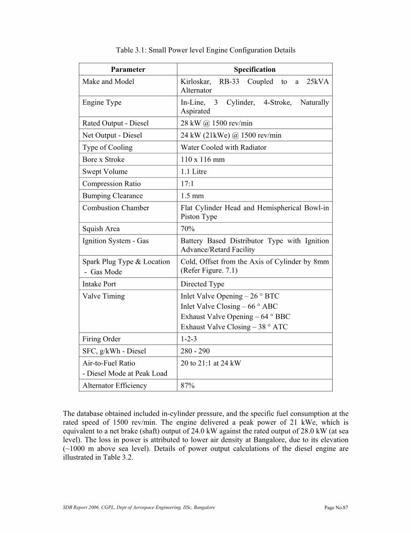
SDB Report 2006, CGPL, Dept of Aerospace Engineering, IISc, Bangalore Page No.87
Table 3.1: Small Power level Engine Configuration Details
Parameter Specification Make and Model Kirloskar, RB-33 Coupled to a 25kVA
Alternator Engine Type In-Line, 3 Cylinder, 4-Stroke, Naturally
Aspirated Rated Output - Diesel 28 kW @ 1500 rev/min Net Output - Diesel 24 kW (21kWe) @ 1500 rev/min Type of Cooling Water Cooled with Radiator Bore x Stroke 110 x 116 mm Swept Volume 1.1 Litre Compression Ratio 17:1 Bumping Clearance 1.5 mm Combustion Chamber Flat Cylinder Head and Hemispherical Bowl-in
Piston Type Squish Area 70% Ignition System - Gas Battery Based Distributor Type with Ignition
Advance/Retard Facility Spark Plug Type & Location - Gas Mode
Cold, Offset from the Axis of Cylinder by 8mm (Refer Figure. 7.1)
Intake Port Directed Type Valve Timing Inlet Valve Opening – 26 ° BTC
Inlet Valve Closing – 66 ° ABC Exhaust Valve Opening – 64 ° BBC Exhaust Valve Closing – 38 ° ATC
Firing Order 1-2-3 SFC, g/kWh - Diesel 280 - 290 Air-to-Fuel Ratio - Diesel Mode at Peak Load
20 to 21:1 at 24 kW
Alternator Efficiency 87%
The database obtained included in-cylinder pressure, and the specific fuel consumption at the rated speed of 1500 rev/min. The engine delivered a peak power of 21 kWe, which is equivalent to a net brake (shaft) output of 24.0 kW against the rated output of 28.0 kW (at sea level). The loss in power is attributed to lower air density at Bangalore, due to its elevation (~1000 m above sea level). Details of power output calculations of the diesel engine are illustrated in Table 3.2.

SDB Report 2006, CGPL, Dept of Aerospace Engineering, IISc, Bangalore Page No.88
Table 3.2: Diesel Engine Net Output Calculations
A Rated shaft output at sea level. The rated output includes power consumed
by the accessories namely, water pump with fan, dynamo, fuel injection pump (FIP).
28.0 kW
B Air pressure at Bangalore is 690 mm HG. De-rating on account of elevation is 9.3%
2.60 kW
C Power consumed by accessories like water pump with fan and dynamo. This was measured by external motoring and is exclusive of power consumed by the FIP.
1.30 kW
D Net shaft output available = A - (B+C) 24.1 kW E Net shaft output (Inclusive of the power consumed by FIP, which is
assumed) 24.0 kW
Conversion Methodology Modifications carried on the diesel engine in order for it to work as a SI engine are as follows.
Insertion of spark plug in place of fuel injector as shown in Plate 3.2. This called for enlarging the diameter of the recess and tapping of appropriate thread (M10) in the cylinder head to receive the spark plug. Modification was done in such a way that the tip of spark plug was in flush with the cylinder head. The location of the spark plug was retained at central position with respect to the combustion chamber. At the time of conversion, hot spark plugs (Product No. W8DC, MICO make) were chosen with an intention of avoiding frequent fouling of spark plugs, but this led to problem of backfiring into the intake manifold at higher power output. It took sometime to identify the cause for the backfire and was later traced to the malfunctioning of the hot spark plug (acting like a hot spot) beyond a certain load (> 16 kW). The problem was subsequently resolved by installing cold spark plugs (Product No. W5DC, MICO make).
Plate - 3.2: Instrumentation on SPE
Fuel Injector Replaced with Spark Plug; Provision Made for Pressure Measurement on the Cylinder Head Shown by the Red Arrow.

SDB Report 2006, CGPL, Dept of Aerospace Engineering, IISc, Bangalore Page No.89
Adaptation of a three-cylinder distributor type battery based ignition system. The fuel injection pump was left intact with an intention of reserving the possibility of modifying back to a diesel engine in a short span of time (less than one hour). This called for additional provision whereby a gearbox was specifically designed to drive the mechanical ignition system’s distributor at camshaft speed. Also provision was made to advance/retard the ignition timing. The diesel fuel injection pump had no role in the operation of gas engine. These details are depicted in Plate 3.3.
Plate - 3.3: Ignition system on SPE
Battery Based Mechanical Ignition System Fitted on the Camshaft Drive; Red Arrow Pointing Towards Provision for Manual Advance/Retard of Ignition Timing. Diesel Fuel Injection Pump (FIP) is also Evident (Right).
The combustion chamber design comprising of a flat cylinder head and slightly offset bowl-in-piston was retained. Changing the thickness of cylinder head gasket altered the clearance volume and hence different CRs were simulated. The combustion chamber along with the cylinder head showing the location of valve and spark plug is shown in Plate 3.1.
Instrumentation on the Engine p - θ Measurements Figure. 3.2 depicts the instrumentation scheme adopted for the experiments. For combustion diagnostics, the in-cylinder pressure was measured using a Piezo sensor (PCB make) mounted on the cylinder No. 1 of the engine. The sensor is hermitically sealed (model No. HS 111A22) with a built-in charge amplifier, the other specifications
Clean producer gas from the gasifier plant Gas Engine
Gas composition &Gas flow rate
Air flow rate
Alternator
Gaseous emissions(NOx, CO)
Power output
In-cylinder pressure(Piezo sensor)
Figure. 3.2 Scheme for Instrumentation

SDB Report 2006, CGPL, Dept of Aerospace Engineering, IISc, Bangalore Page No.90
being: resolution - 0.69 kPa, rise time < 1 micro second, discharge time constant > 500 second, natural frequency of the crystal = 550 kHz. The in-cylinder pressure measurement synchronized with the crank angle measurement (sensed using an optical sensor) was acquired on a PC (Personal Computer, 600 MHz processor) at time intervals of one-degree crank angle. The piezo sensor could not be flush mounted with the interior part of the combustion chamber due to constraints on the engine cylinder head. However, the sensor was mounted by drilling a 1.0 mm size hole in the cylinder head, and a 40 mm long aperture communicated between the sensor and the combustion chamber. This therefore introduced a time lag between the actual pressure changes in the combustion chamber and the pressure sensed by the sensor (due to 40 mm long passage). The time lag is estimated to be of the order of 0.4° CA. In addition to this, the error in TC identification (explained in the following section) is about 0.2° CA, which adds to a total of 0.6° CA in terms of accuracy of pressure-crank angle data recorded. This aspect is considered while interpreting the results. Accuracy of TC Identification The Top center (TC) has been identified in accordance to the procedure discussed by Lancaster et al [1975]. To locate TC within accuracy of 0.1° CA, the authors have identified a systematic procedure, wherein multiple readings are required to be taken on either sides of TC (at 40° CA). The above-mentioned procedure has been adopted for TC identification and therefore accuracy in the current case should be well within 0.1° CA. Emission Measurement The emissions and exhaust temperature were measured in the exhaust manifold; the temperature was measured using K-type (Chromel-Alumel) thermocouple. Adequate provision was made to condition the flue gas sample prior to measurements. The flue gas composition was analyzed using a multi-component analyzer, which are based on infrared and chemical cell technique. The substances analyzed were nitrogen oxide (NO), carbon monoxide (CO), carbon dioxide (CO2) and oxygen (O2) on an intermittent basis. Since the input feed was gas with particulate matter averaging about 60 mg/Nm3
, this would amount
less than 25 mg/Nm3 (some particulate matter would burn) in the exhaust (air-to-fuel gas ratio
~1.3). Therefore particulate measurement was not envisaged. Air/Gas Flow Measurement The air and gas flow (in the case of gas engine) were separately measured using calibrated venturimeters. The venturimeters were subjected to primary calibration by adopting standard pitot tube measurement procedure. Power Output Measurement The engine output was measured by recording the voltages across the three phases of the alternator and the current drawn by the load bank. The load bank consisted of a number of resistor coils of 1.0 and 0.5 kWe each, totally to about 25 kWe. Digital frequency meter was employed to the record the frequency of the output.

SDB Report 2006, CGPL, Dept of Aerospace Engineering, IISc, Bangalore Page No.91
Instrumentation on the Gasifier The producer gas constituents were measured using on-line gas analyzers on a continuous basis. The sample gas was analyzed using a multi-component analyzer comprising of hydrogen (H2), carbon monoxide (CO), methane (CH4), carbon dioxide (CO2) and oxygen (O2) detecting sensors. The measurements of CO, CH4 and CO2 fractions are based on infrared technique, H2 on thermal conductivity technique and the O2 on chemical cell. Calibration gas of a composition similar to that of a producer gas was used for calibrating the gas analyzer prior to start and close of every test run. Random calibration was also performed between the runs in order to reduce the errors. The commercially sourced calibration gas (from Bhoruka gases Ltd, Bangalore) has been primarily calibrated using gas chromatography. The sample producer gas was conditioning prior to commencement of measurements. This was achieved in two stages using moisture and particulate matter filtering system. The data obtained from gas analyzers in terms on gas constituents/composition was further used for estimation of calorific value of producer gas and this provided an input for estimation of energy density of producer gas-air mixture. Experimental Procedure As mentioned earlier, the well-researched, tested and industrial version of the gasifier of 75 kg/hr rating formed the gas generator. The system has qualified for long hours of continuous operation in meeting the industrial requirements in terms of generation of consistent quality gas. The system comprised of a reactor, gas cooling and cleaning system, flare and ducting to the gas engine. The reactor and cooling system are similar to the discussed in Chapter II. However, in the gas cleaning system instead of using chilled water for scrubber a diesel wash was provided. The chilled water scrubbing system is a later development in gasification system and is the part of the system for the medium power level engine (MPE) experiments. The details of these individual sub-systems have been discussed earlier in Chapter II, however an overall schematic of 75 kg/hr is shown in Figure. 3.3. Commencement of Testing The gasification process was initiated by lighting the reactor with an open flame at the air nozzles. The gas drawn by the blower was ducted to the flare. Within about ten to fifteen minutes, combustible gas was generated, with oxygen level in the product gas falling close to zero. This event marked the completion of gasification process, further to which the gasifier is operated in flare mode until the system reached steady state of operation. Typically this was about 2-3 hours from the cold start. The producer gas composition was monitored during this period and at the time of start of the gas engine the composition was typically be 19+1% H2, 19+1% CO, 2+0.5% CH4, 12+1% CO2 and the rest, N2, which corresponded to energy content of 5.20 – 5.50 MJ/Nm3. Standard biomass namely, causurina with moisture content of 12-15% on dry basis (sun-dried biomass) was used as the feedstock to obtain consistent quality gas. Once the gas composition stabilized, the engine was operated for few minutes at 1500 rev/min under no-load condition. Subsequent operations on load were also conducted at 1500 + 50 rev/min. The throttling for speed control and air-to-fuel proportioning was achieved using manually operated valves (without carburetor). Experiments were conducted at CRs of 17.0, 14.5, 13.5 and 11.5. The CR values are based on cylinder’s geometric measurements. The engine was tested at different ignition timing settings to determine the optimum ignition
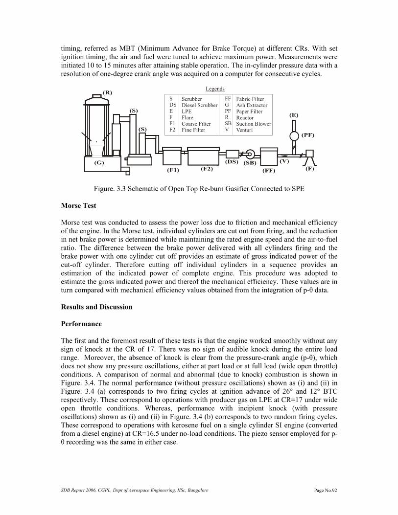
SDB Report 2006, CGPL, Dept of Aerospace Engineering, IISc, Bangalore Page No.92
timing, referred as MBT (Minimum Advance for Brake Torque) at different CRs. With set ignition timing, the air and fuel were tuned to achieve maximum power. Measurements were initiated 10 to 15 minutes after attaining stable operation. The in-cylinder pressure data with a resolution of one-degree crank angle was acquired on a computer for consecutive cycles.
Legends
ScrubberDiesel ScrubberLPEFlareCoarse FilterFine Filter
S DS E F F1 F2
FF G PFR SB V
Fabric FilterAsh ExtractorPaper FilterReactorSuction BlowerVenturi
Figure. 3.3 Schematic of Open Top Re-burn Gasifier Connected to SPE Morse Test Morse test was conducted to assess the power loss due to friction and mechanical efficiency of the engine. In the Morse test, individual cylinders are cut out from firing, and the reduction in net brake power is determined while maintaining the rated engine speed and the air-to-fuel ratio. The difference between the brake power delivered with all cylinders firing and the brake power with one cylinder cut off provides an estimate of gross indicated power of the cut-off cylinder. Therefore cutting off individual cylinders in a sequence provides an estimation of the indicated power of complete engine. This procedure was adopted to estimate the gross indicated power and thereof the mechanical efficiency. These values are in turn compared with mechanical efficiency values obtained from the integration of p-θ data. Results and Discussion Performance The first and the foremost result of these tests is that the engine worked smoothly without any sign of knock at the CR of 17. There was no sign of audible knock during the entire load range. Moreover, the absence of knock is clear from the pressure-crank angle (p-θ), which does not show any pressure oscillations, either at part load or at full load (wide open throttle) conditions. A comparison of normal and abnormal (due to knock) combustion is shown in Figure. 3.4. The normal performance (without pressure oscillations) shown as (i) and (ii) in Figure. 3.4 (a) corresponds to two firing cycles at ignition advance of 26° and 12° BTC respectively. These correspond to operations with producer gas on LPE at CR=17 under wide open throttle conditions. Whereas, performance with incipient knock (with pressure oscillations) shown as (i) and (ii) in Figure. 3.4 (b) corresponds to two random firing cycles. These correspond to operations with kerosene fuel on a single cylinder SI engine (converted from a diesel engine) at CR=16.5 under no-load conditions. The piezo sensor employed for p-θ recording was the same in either case.

SDB Report 2006, CGPL, Dept of Aerospace Engineering, IISc, Bangalore Page No.93
0
40
80
120
340 360 380 400 420
(i)
(ii)
(a)
Producer Gas
Ign Timing(i) 26o BTC(ii) 12o BTC
0
40
80
120
340 360 380 400 420
(i)
(ii)
(b)
(i) & (ii) : Random cyclesKnock
Kerosene
Figure. 3.4 (a) Normal Combustion under Wide Open Throttle Condition with Producer Gas
at Different Ignition Timings at CR=17, (b) Incipient Knock with Kerosene at No-Load Condition with Ignition Timing of 30° BTC at CR=16.5.
The results of the power output with producer gas are shown in Table 3.3. At CR=17, the engine delivered a maximum net brake output of 20 kW (17.5 kWe) at an efficiency of 30.7% compared to 24 kW (21 kWe) brake output at 33% efficiency with diesel (compression ignition mode). The efficiency calculation is based on the ratio of net brake output to the energy content of the air and gas mixture. The useful output and efficiency decreased with the lowering of CR. A maximum net brake output of 17.6 kW (15.3 kWe) at an efficiency of 27.5% was obtained at CR of 11.5. The power output at intermediate CR of 14.5and 13.5 were 18.8 and 18.6 kW respectively and with efficiencies around 29%. The efficiency at CR = 13.5 was comparable to that at 14.5 probably due to relatively leaner operation. The extent of de-rating in brake power was about 16.7% at CR = 17 and increased to as high as 26% at CR = 11.5 compared with baseline operations in diesel mode.
Table 3.3: Maximum Net Engine Output at Varying CR
CR IGN, BTC
Φ Net Elec. Power, kWe
Net Brake Power
(BPNet) , kW
Mixture Energy Density, MJ/kg
Efficiency : Gas-to-Shaft,
% 17.0 06 1.10 17.5 20.0 2.20 30.7 14.5 10 1.10 16.4 18.8 2.20 29.0 13.5 14 1.06 16.2 18.6 2.10 29.3 11.5 15, 17 1.07 15.3 17.6 2.20 27.5
Φ =Equivalence Ratio: (Actual fuel- to- air ratio)/(Stoichiometric fuel- to- air ratio)

SDB Report 2006, CGPL, Dept of Aerospace Engineering, IISc, Bangalore Page No.94
Table 3.4: Maximum Net Engine Output as a Function of Ignition Timing at Varying CR
IGN, BTC
Φ BPnet, kW* η : Gas–to-Shaft, %
IGN, BTC
Φ BPnet, kW* η : Gas–to-Shaft, %
CR=17.0 CR=14.5
06 1.10 20.0 30.8 08 1.20 18.6 25.0
12 1.00 19.8 31.0 10 1.10 18.8 29.0
17 1.09 18.4 29.0 16 1.11 17.9 27.5
22 1.03 17.9 28.0 20 1.11 17.7 27.2
26 1.10 16.2 25.3
33 1.25 14.0 19.0
CR=13.5 CR=11.5
08 1.05 18.2 28.6 06 1.07 17.0 27.0
14 1.06 18.6 29.0 15,17 1.07 17.6 27.5
18 1.07 17.0 27.8 27 1.09 15.6 25.5
25 1.06 17.0 28.0 38 1.07 13.3 20.0
* Excluding Radiator Fan Power
The net brake output with producer gas at varying ignition timing for the four different CRs tested is shown in Table 3.4. It is evident from the above data that ignition timing had to be retarded with the increase in CR in order to obtain higher output. This is because the thermodynamic conditions in terms of pressures and temperature are more severe at higher CR and thereof the combustion is faster thus calling for the optimum ignition timing to be located close to TC. The maximum output was recorded at an ignition advance of 6° BTC at CR=17 and increased to about 15 - 17° BTC at a CR=11.5. At intermediate CR of 14.5 and 13.5 the ignition advance was 10 and 14° BTC respectively. The fuel-air equivalence ratio was about 1.06 + 0.5 in most of the cases, with efficiency of 30.7 and 27.5% corresponding to maximum output at higher and lower CRs respectively. An isolated case of efficiency at 31% was seen corresponding to ignition setting of 12° CA, probably due to relatively leaner operation. In the above data presented, the air-to-fuel ratio was tuned from the viewpoint of deriving maximum output and therefore the efficiency figures are necessarily not the maximum that can be obtained. The incremental gain in maximum power and efficiency per unit CR is shown in Table-3.5. The gain in power was between 2.2 and 2.6 per unit CR, but the gain in efficiency was marginally lower. However, these figures are well within the range of 1 to 3% gain per unit increment of CR reported by Heywood [1988].
Table 3.5: Incremental Gain in Power and Efficiencies
Range in CR Gain in power/CR, % Gain in efficiency/CR, % 14.5 to 17.0 2.60 2.3 13.5 to 17.0 2.20 1.4 11.5 to 17.0 2.50 2.1

SDB Report 2006, CGPL, Dept of Aerospace Engineering, IISc, Bangalore Page No.95
Next, the variation of mechanical efficiency (ratio of net brake power to gross indicated power), ηmech with CR is shown in Table 3.6. These values are deduced from indicated power measurements (based on integration of pressure-volume diagram) and net output measured, also values obtained from standard multi-cylinder Morse test are shown in Table.3.6. The ηmech of the engine at CR of 17 is about 80% and increased to as high as 87% at CR of 11.5. The increase in ηmech is attributed to the reduction in rubbing friction [Gish et al, 1958] due to lower cylinder pressures encountered at lower CRs. A break-up of the components leading to total losses is further discussed in Table 7.3 of Chapter VII.
Table 3.6: ηmech Measurements
CR
ηmech from
∫ pdVηmech from – Morse test
17.0 80-82 81 + 1 14.5 84-86 84 +2 13.5 85-88 86 +2 11.5 88-90 88 +1
Pressure – Crank Angle Data The pressure-crank angle (p-θ) recording is shown in Figure 3.5 to 3.8 at different CRs, none of these show any trace of knock for all ranges of load inclusive of peak. These figures contain ensemble average data over thirty consecutive cycles.
0
20
40
60
80
300 320 340 360 380 400 420
Crank Angle, degree
Cyl
inde
r Pr
essu
re, b
ar
Black : FiringGrey : Motoring
26o CA
22o CA
17o CA
12o CA
6o CA33o CA
Figure. 3.5 p-θ Recording Corresponding to Maximum Brake Output at Varying Ignition Advance at CR=17. Ensemble-Averaged Data Over 30 Consecutive Cycles.

SDB Report 2006, CGPL, Dept of Aerospace Engineering, IISc, Bangalore Page No.96
0
20
40
60
300 320 340 360 380 400 420
Crank Angle, degree
Cyl
inde
r Pr
essu
re, b
ar
Black : FiringGrey : Motoring
16o CA
20o CA
8o CA
Figure 3.6: p-θ Recording Corresponding to Maximum Brake Output at Varying Ignition Advance at CR=14.5. Ensemble-Averaged Data Over 30 Consecutive Cycles.
0
20
40
60
300 320 340 360 380 400 420
Crank Angle, degree
Cyl
inde
r Pr
essu
re, b
ar
Black : FiringGrey : Motoring
14o CA
25o
18o CA
Figure 3.7: p-θ Recording Corresponding to Maximum Brake Output at Varying Ignition Advance at CR=13.5. Ensemble-Averaged Data Over 30 Consecutive Cycles.

SDB Report 2006, CGPL, Dept of Aerospace Engineering, IISc, Bangalore Page No.97
0
20
40
60
300 320 340 360 380 400 420
Crank Angle, degree
Cyl
inde
r Pr
essu
re, b
ar
Black : FiringGrey : Motoring
27o CA16o CA
6o CA
38o CA
Figure 3.8: p-θ Recording Corresponding to Maximum Brake Output at Varying Ignition
Advance at CR=11.5. Ensemble-Averaged Data Over 30 Consecutive Cycles. It is clear from these curves that smooth and normal combustion seemed to occur even at advanced ignition timing of 33° CA corresponding to CR of 17. Faster burn rate due to presence of hydrogen in the fuel gas could be the principal factor for the no-knock performance. The effect of the ignition advance on the pressure history is evident from the above curves. There are substantial differences in the maximum cylinder pressure and their point of occurrence. The ratio of maximum cylinder pressure between the highest and the lowest CR at corresponding ignition timing is about 2. The net work delivered over a complete cycle can be found by integrating the pressure-volume (p-v) data over the four processes. This also helped in identifying the optimum ignition timing for a given CR - commonly referred as MBT. The net indicated mean effective pressure (IMEP) obtained from the integrated p-v data is a measure of effectiveness with which an engine of a given volumetric displacement converts the input energy into useful work. The IMEP obtained from ensemble average p-v data (~ 30 cycles) at varying CR as a function of ignition timing is shown in Figure 3.9. At CR=17, the maximum IMEP recorded is 5.98 bar corresponding to a ignition timing of 6° CA and this declined to 4.85 bar with ignition timing being 15° CA at CR of 11.5. These values are obtained at � = 1.08 + 0.2 and fall within the anticipated value of � = 1.0 to 1.1 [Heywood, 1988]. It is also evident from the plot that variations in the IMEP values are modest between ignition timings of 6 and 12° CA corresponding to CR=17. Exploring further the p-θ data, the peak pressure and the point of occurrence at ignition timings close to MBT are listed in Table 3.7. These measurements are accurate within – 1.0° CA (due to possible lag in the signal and error in TC identification). It is evident from the data that peak pressure seemed to occur between 17 and 19° ATC (After Top Centre) at all CRs. In the case of CR=13.5, the peak pressure seemed to occur at the optimum value (17° ATC) identified in the literature [Heywood, 1988; Wu et al, 1993]. In the case of CR=11.5, the peak pressure occurred at 17 and 12° ATC for an ignition timing of 15 and 17° BTC respectively. The difference in the IMEP between the two ignition timings was found to be 3%. However, for CR of 17 and 14.5 the ignition timing identified in the Table 3.7 seemed to

SDB Report 2006, CGPL, Dept of Aerospace Engineering, IISc, Bangalore Page No.98
be marginally deviating from the optimum value. The variation of IMEP within this close range would be marginal as it is well acknowledged that the relative torque delivered has a flatter characteristic around MBT [Heywood, 1988].
Table 3.7: Cylinder Peak Pressures and Their Occurrence
CR Ign. advance ° CA
Peak pressure, bar
Occurrence ° ATC
17.0 6 55.00 20 14.5 10 43.30 19 13.5 14 45.00 17 11.5 15, 17 33.00, 38.00 17, 12
The coefficient of variation of the IMEP at all CRs and ignition settings occurred well within 3-3.5%, as shown in Figure 3.10 implying low cycle-to-cycle variation. The reason for low cyclic variation is the faster rate of combustion occurring inside the engine cylinder. The faster rate of combustion is attributed to higher flame speeds due to the presence of hydrogen in the gas and also to the combustion chamber design.
3
4
5
6
7
0 5 10 15 20 25 30 35 40
Ignition Advance, oCA
IME
P, b
ar
CR=17.0CR=14.5CR=13.5CR=11.5
Figure 3.9: Variation of IMEP (Net) with Ignition Advance at Various CRs

SDB Report 2006, CGPL, Dept of Aerospace Engineering, IISc, Bangalore Page No.99
0
1
2
3
4
0 5 10 15 20 25 30 35 40Ignition advance, o CA
CO
V o
f IM
EP,
%
CR=17.0
CR=14.5
CR=13.5
CR=11.5
Figure 3.10: COV of IMEP (Net) with Ignition Advance at Various CRs
0
20
40
60
80
240 280 320 360 400 440 480
Crank Angle, degree
Cyl
inde
r Pr
essu
re, b
ar
CR=14.5
CR=17.0(Diesel)
CR=17.0
CR=13.5
CR=11.5
377
Figure 3.11: Comparison of p-θ Curves at Different CR; Ignition Timing is at MBT or Close to MBT (Within MBT + 2° CA). The p—θ curves correspond to ignition setting of 10°, 10°, 14° and 15° BTC for CR of 17, 14.5, 13.5 and 11.5 respectively. Operation in Diesel Mode at 90% of rated Load (at Optimum Injection Timing - 34° BTC). All are Ensemble-Averaged Data over 30 Consecutive Cycles.

SDB Report 2006, CGPL, Dept of Aerospace Engineering, IISc, Bangalore Page No.100
Figure 3.11 shows the comparison of p-θ curves for different CR around MBT in gas mode of operation. In case of the ignition timing close to MBT, the peak pressure is observed to occur around 16 -17° ATC. The ratio of maximum cylinder pressure between the highest and the lowest CR is about 2. The p-θ curve in diesel mode at MBT shows a maximum pressure of 85 bar to occur at 10°ATC. The point of occurrence of peak pressure is consistent with the data (5 -10° ATC) available in literature [Heywood, 1988]. The observed difference in the p-θ curves between diesel and gas mode is attributed to the nature of combustion. In case of diesel mode, combustion occurs in a diffusion mode, wherein fine droplet combustion occurs in an atmosphere of vitiated air. The pressure rises rapidly to a peak at 10° ATC since the initial rate of burning is fast. Whereas in gas operation (which is essentially in spark ignition mode of operation), combustion occurs in a pre-mixed mode, wherein there is a definite flame front traveling across the pre-mixed fuel - air mixture. Therefore the pressure rise in this case is not as rapid as seen with compression ignition mode of operation. It is also evident from these curves the magnitude of pressure rise is lower in case of gas operation. Summarizing, the MBT for producer gas fuel is identified to be in the following crank angle intervals. 6-10° BTC for CR=17.0, 10-12° BTC for CR=14.5, 12-14° BTC for CR=13.5 and 15 –17° BTC for CR=11.5. This range is identified keeping in view the modest variation in the net power output.
0
15
30
45
% o
f Inp
ut E
nerg
y
PG 32.9 30.1 37.0Diesel 34.6 35.4 30.0
1 2 3Gross brake output Exhaust Coolant & Miscl.
Figure 3.12: Energy Balance Comparison in Diesel and Producer Gas Mode at Maximum Brake Output. The Marker Refers to the Error Band.
Energy Balance Figure 3.12 represents the overall energy balance at CR =17. The energy balance is based on gross brake power output. The gross brake output is sum of net shaft output and power consumed by engine accessories (water pump/fan, dynamo and FIP = 1.4 kW). The energy

SDB Report 2006, CGPL, Dept of Aerospace Engineering, IISc, Bangalore Page No.101
balance in gas mode corresponding to maximum brake output (at 6° CA) showed a useful output (Gross brake power) of 32.9%, about 30% is lost through exhaust (sensible and chemical enthalpy - CO) and remaining 37% to the cooling water (inclusive of frictional and radiative losses). Figure 3.12 also compares the energy balance in gas and diesel mode (at rated output of 24kW) at CR of 17, the energy loss to the coolant and miscellaneous is about 37% compared to 30% in diesel and whereas, energy loss through exhaust is lower by about 5% in gas mode. Overall the brake thermal efficiency is lower by about 1.5% in gas. The energy balance as a function of CR is shown in Figure 3.13. There is an increase in energy loss through exhaust with the reduction in the CR, where as the loss through the coolant is higher at higher CR. The increased amount of heat loss to the cooling water in gas operations is attributed to engine combustion chamber design. Heywood [1988] indicates that engine geometries such as bowl-in-piston would experience 10% higher heat transfer. The heat transfer to the coolant in the current case falls well within this range (7-10%). The influence of engine geometry on heat loss could
0
15
30
45
% o
f Inp
ut E
nerg
y
Brake output 32.9 31.5 31.8 29.7Exhaust 30.2 35.3 37.8 45.0Coolant & Miscl. 36.9 33.2 30.4 25.3
1 2 3 417 14.5 13.5 11.5CR
Figure 3.13: Comparison of Energy Balance at Various CRs with Producer Gas Corresponding to Maximum Brake Output. The Marker Refers to the Error Band.
be more in gas mode compared to diesel because of basic difference in the nature of combustion. In the case of compression ignition engine, combustion is heterogeneous and essentially occurs at multiple ignition sites in a diffusion mode. Therefore, there is no definite flame front propagation and combustion does not occur close to the wall unlike that in a spark-ignition engine. This is one of the prime reasons for increased heat loss to the coolant in spark-ignition engine, which is so in the current study in gas mode. With the increase in CR, it can be seen that there is marginal improvement in the conversion efficiencies. However, in reality the gain in efficiency is much larger at higher CR and consistent with the thermodynamics. The gross indicated efficiency (including pumping losses) at CR=17 (39%) is higher by about 18% compared to that at CR=11.5 (33%).

SDB Report 2006, CGPL, Dept of Aerospace Engineering, IISc, Bangalore Page No.102
However, the gain is reduced due to lower mechanical efficiency at higher CR as shown in Table - 3.6. Similarly, energy loss to the coolant is higher at higher CR due to higher cylinder temperature (as a consequence of higher cylinder pressure) and increased frictional losses (refer Table 7.2 and discussion therein) and energy loss through exhaust decreases with the increase in CR due to increased thermal efficiency. Emissions The emissions measured are Nitric oxide (NO) and Carbon Monoxide (CO). The variation of NO in gas mode at varying CR with ignition advance is shown in Figure. 3.14. NO2 was not accounted as it forms small part (~5%) of NOx generated [Heywood, 1988]. The NO level has been represented as an emission index in units of gram per unit MJ of input energy. These results are compared with the CPCB norms (equivalent to EURO I norm) meant for diesel engine powered vehicle, as there are no existing CPCB norms for stationary engines. Similarly, there are no norms existing for small power level (< 2.0 MW) stationary engines, therefore, existing diesel vehicular norms of CPCB are stated for comparison. Also the data is compared with the Swiss emission norm, as it is generally understood that their norms are stringent. The NO level reduced with the retardation of ignition timing and this feature is observed for all CRs. The NO level is observed to be maximum at the highest CR with advanced ignition timings, whereas in the MBT range of 6 to 20° BTC the NO is lower and comparable in almost all the cases. It is well known that NO generation is strongly dependent on the temperature, oxygen availability and residence time in the combustion chamber. With the flame speed of the gas mixture being high, the ignition setting is retarded whereby the residence time in the high temperature combustion chamber is automatically reduced. Therefore the low NO levels at retarded ignition setting are an expected and consistent behavior. The above results match well with those quoted by Heywood [1988], which show small to modest variation of NO with CR. The NO emissions are lower than the CPCB and Swiss norm for all cases around MBT.
0.0
0.2
0.4
0.6
0.8
1.0
0 5 10 15 20 25 30 35 40
Ignition advance, oCA
NO
, g/M
J
0 0.4 0.8 1.2 1.6 2 2.4 2.8 3.2 3.6 4 4.4Time, millisecond
CR = 17.0CR = 14.5CR = 13.5CR = 11.5
MBT Timing
Swiss Norm
CPCB (India) norm : 2.22 g/MJ
Figure 3.14: Variation of NO with Ignition Advance at Various CRs

SDB Report 2006, CGPL, Dept of Aerospace Engineering, IISc, Bangalore Page No.103
0
5
10
15
20
0.95 1 1.05 1.1 1.15
Fuel-air equivalence ratio
CO
, g/M
JCR = 17.0CR = 11.5
6
22
26, 17
10,12
14
27
6
16, 38
CPCB - 1.25 g/MJ
Swiss - 0.32 g/MJ
Figure 3.15: Variation of CO with Fuel-Air Equivalence Ratio. The Number Next to the
Legend Indicates the Ignition Advance in ° CA, BTC. The variation of CO with equivalence ratio (Φ) is shown in Figure 3.15. The CO levels are represented in grams per MJ of input energy. The trend of CO with Φ is clear from the figure. The CO levels were lower at the highest CR as well as fuel lean conditions, and this could be attributed to higher temperatures, leading to relatively complete combustion. Overall, the levels are found to be much higher than the CPCB and Swiss norm. It appears that the engine can meet CPCB and other emissions norms (Table 3.11) if the engine is operated at fuel lean conditions without the need for a catalytic convetor. Concluding Remarks Performance of the engine at higher CR is smooth and it has been established that operating engines using producer gas in SI mode at CR up to 17 is feasible. This is obvious from the p-θ curve, which shows smooth rise in pressure without any pressure oscillations. A shorter duration of combustion has been observed with producer gas fuel, requiring retardation of the ignition timing to achieve MBT. These faster burning cycles are corroborated by low cyclic pressure fluctuations with coefficient of variation ~ 3%. The faster burning process has been identified to be due to higher flame speed of the fuel - air mixture and this is attributed to the hydrogen content in the gas. The MBT arrived from this study is much retarded than claimed by the earlier researchers. The MBT in the current case are in the range between 6 and 17° CA for CR range between 17 and 11.5 against 30 - 45° CA (for a CR of 11.5 and below) claimed by the earlier researchers. This change in ignition advance in the present study can only be attributed to the improved producer gas composition. The hydrogen content in the present case is about 18-20% against 11-12% claimed by Parke et al [1981] and 10% (theoretical) by Martin et al [1981]. However, it is difficult to comment on the retarded MBT of 35° CA claimed by Shashikanta et al [1999] with hydrogen content of 24%.

SDB Report 2006, CGPL, Dept of Aerospace Engineering, IISc, Bangalore Page No.104
The maximum de-rating in power is observed to be 16.7% in gas mode compared to diesel operations at comparable CR. The extent of de-rating is much lower when compared to any of the previous studies [Parke et al 1981, Ramachandra, 1993, Martin et al, 1981]. This value matches with a similar kind of de-rating reported with natural gas operation by Das et al [1997]. However, the brake thermal efficiency drops down by 5% compared to normal diesel mode of operation. This is related to excessive heat loss to the coolant at all CRs, resulting in engine overheating within 30-40 min of operations at full load. The emission in terms of NO is found to be much lower than the stipulated norms of CPCB and Swiss. However, the CO levels are found to higher. These observations are consistent with the results of Giordano [1999] on a producer gas engine powered with a IISc gasifier. Lastly, the information that is relevant to biomass gasifier coupled to a gas engine is the specific fuel (biomass) consumption. The specific biomass works out to about 1.15 –1.25 per kWh electric energy generated that corresponds to an overall efficiency (biomass to electricity) of 21 and 19% at 17 and 11.5 CR respectively. Medium Power level Experiments Description of the Engine The understanding gained from the experimental work on the SPE engine is translated on to the medium power level engine (MPE) and its performance accessed on producer gas. The gas engine chosen for experiments is a 12 cylinder (V-configuration), turbo-charged – after cooler engine, supplied originally to operate on dilute natural gas (biogas fuel). These brand engines are marketed as bio-gas engines and are serving as base load power plants in many parts of India. This engine is adopted to operate on producer gas along with a specially designed gas carburetor. The detailed specification of the engine is given in Table 3.8. This engine is basically built from a diesel engine frame (model no. TBD4V12, rated at 444 kW at CR of 15) at a modified CR of 12, to operate on gaseous fuels in a spark-ignited mode. The other modifications implemented on the engine are with respect to turbo-charger (model K-28 in place of K-36) and combustion chamber (simple cylindrical bowl in place of torroidal shape). The K-36 and K-28 turbo-charger are designed to generate a pressure ratio of 2.2 and 1.5 - 1.6 respectively. Therefore, the estimated power rating of the modified engine in diesel is between 290 - 310 kW (with the modified turbo-charger and lower CR ~ 2% reduction in power per unit CR assumed from Heywood [1988]). The modified engine (to operate as a SI engine) was initially equipped with double sparking ignition system, where in a redundant spark occurred during the exhaust process. Itso happened that whenever the engine was operated with an ignition timing coinciding with the valve overlap period, a backfire occurred into the engine intake. This therefore limited the available range of ignition timing for testing purposes. The problem was subsequently resolved by replacing with a single sparking ignition system, which permitted engine operation over a wider range of ignition timing.

SDB Report 2006, CGPL, Dept of Aerospace Engineering, IISc, Bangalore Page No.105
Table 3.8 Medium Power level Engine Configuration Details
Parameter Specification Make and Model Greaves, Coupled to a 300 kVA Alternator Engine Type 12 Cylinder, ‘V’ Configuration Gas Engine, Turbo-Charged
with After Cooler Rated Output - Diesel 290 – 310 kW (Estimated) @ 1500 Rev/Min Rated Output – Diluted Natural Gas (Bio-Gas)
250 - 270 kW @ 1500 Rev/Min (Achieved)
Type of Cooling Water Cooled with Radiator Bore x Stroke 128 x 140 mm Swept Volume 1.8 Litre Compression Ratio 12:1 Bumping Clearance 1.6 mm Combustion Chamber Flat Cylinder Head and Bowl-in Piston Squish Area 68% Ignition System Gill Instruments – Single Sparking Unit with Individual Coil
for Each Cylinder Governor GAC Make Spark Plug Type & Location Cold, Offset – Located in the Vertical Plane Close to the
Outer Edge of the Bowl Intake Port Directed Type Valve Timing Inlet Valve Opening – 12° BTC
Inlet Valve Closing – 55° ABC Exhaust Valve Opening – 44° BBC Exhaust Valve Closing – 15° ATC
Firing Order A1, B5, A5, B3, A3, B6, A6, B2, A2, B4, A4, B1 SFC, m3/kWh – Bio-Gas 0.3 Alternator Efficiency 92%
BTC: Before Top Center ABC: After Bottom Centre BBC: Before Bottom Centre ATC: After Top Centre
The combustion chamber is formed of a flat cylinder head and a bowl-in piston. The bowl is cylindrical in shape and has a squish area of 68% (percentage of piston area closely approaching the cylinder head at the smallest spacing). The spark plug is located at an offset in the vertical plane close to the outer edge of the bowl. The single spark type electronic ignition unit comprised of a controller, Hall effect sensor, and individual ignition coils,

SDB Report 2006, CGPL, Dept of Aerospace Engineering, IISc, Bangalore Page No.106
wiring harness and spark plugs. The ignition timing was precisely controlled by interfacing with a computer to within one-degree crank angle. The engine coupled with a standard alternator was connected to a load bank (resistor coils) to facilitate load tests. The mixture (air + gas) intake system comprised of an air filter, turbo-compressor, after cooler, mixture controller – gas governor, manifold and runner to each cylinder head. A 250-kg/hr-biomass gasifier formed the gas generator with the system elements in terms of gas cleaning system different compared to the 75- kg/hr system. The details of the 250-kg/hr gasifier system has been dealt earlier. Plate 3.4 shows the view of the gasifier.
Plate 3.4: A View of a 250 kg/hr Open-Top, Re-Burn Down Draft Gasifier to Supply Gas to MPE. Major Sub-Systems of the Plant Identified. The Inset on the Right Shows the Gas Engine
Since the engine is of reasonably higher power level, the air-to-fuel control due to load variation assumed a major proposition. This called for design and development of a gas carburetor for producer gas application, as carburetors are not available for producer gas fuel. The carburetors available for other gaseous fuel, namely the natural gas, biogas and landfill gas are unsuitable due to widely different stoichiometric air-to-fuel requirement. The stoichiometric air-to-fuel ratio varies between 10 to 6 (on volume basis) for fuels such as natural gas and bio-gas/land fill gas based on methane content in the gas. However, stoichiometric air-to-fuel ratio for producer gas is about 1.2 to 1.4 (on volume basis), based on the constituents of the gas.

SDB Report 2006, CGPL, Dept of Aerospace Engineering, IISc, Bangalore Page No.107
Producer Gas Carburetor The essential features in the gas carburetor are
• Ability to maintain the required air-to-fuel ratio (1.2 to 1.5:1) with load or throttle variation
• Smooth operation with minimal pressure loss
• Shut off the fuel in case of engine tripping or shut-down
• On-line provision for air/fuel tuning during testing
The above-mentioned feature was incorporated in the development of a gas carburetor and is shown in Figure 3.16. The carburetor is simple in design and does not have moving components. It has a separate port for air and fuel, where the individual ports could be modified or tuned to achieve the required air-to-fuel ratio. The carburetor is designed to operate in conjunction with the zero-pressure regulator. The combination of pressure regulator and gas carburetor was located between the gasifier and the engine intake system as shown in Figure 3.16. The zero pressure regulator ensures a gas pressure (downstream of the pressure regulator) identical to that of air pressure and this is achieved by connecting the air pressure line (down stream of air filter) to the upper chamber of the regulator. This arrangement ensures the regulator to maintain the gas pressure close to that of air pressure (~ a few mm below atmospheric pressure) and thereby the set air/fuel ratio irrespective of the total mixture flow rate.
Producer Gasfrom 250kg/hr Gasifier(at Blower Exit)
Zero pressure regulator
Valve seat
Diaphragm
Atmosphericpressure
Air pressure lineAir filter
Air
Air
Gas
Figure 3.16: Schematic of Producer Gas Carburetor with Zero Pressure Regulator in the Gas-Air Line Circuit

SDB Report 2006, CGPL, Dept of Aerospace Engineering, IISc, Bangalore Page No.108
0.6
0.8
1
1.2
1.4
1.6
1.8
2
100 180 260 340 420
Mixture flow rate, g/s
A/F 30:70
40:60
@ No-load @ 200 kW
Area Ratio for Air & Fuel Entry
Figure 3.17: Flow Tests with Gas Carburetor at Varying Area Ratio for Air and Fuel Entry
Flow tests performed with zero-pressure regulator and the gas carburetor showed reasonable functioning in terms of air-to-fuel ratio control against total or mixture flow rate variations as shown in Figure. 3.17. Flow test was conducted using a blower to simulate the engine suction. The air and fuel flow rates were individually measured over a range of engine’s operating conditions. The two cases shown in the above figure correspond to area ratios for the air and fuel entry. These cases are possibly the extreme limits and the required operation point for the engine operation could lie in between them. The A/F ratio was reasonably constant beyond a specified mixture flow rate, with relatively rich mixture at low mixture flow rates. This characteristic is desirable from the viewpoint of engine operation – rich mixture for engine start-up and no-load operations, relatively leaner mixture during part load operation. However, for peak load operation – stoichiometry or rich mixture is desired calling for the adjustment of the carburetor flap. Considering gas engine operation at the field level, the carburetor is designed in such a manner that in the event of load throw-off the flap of the carburetor could move to full air flow (by motorizing) condition thus ensuring safety of the engine. Experimental Procedure The scheme of operation up to the exit of gas from the gasifier system was on lines similar to that mentioned for SPE. However, instead of engine drawing the gas, the gas was drawn using a blower and made available for the engine operation. The gas was made available at a higher pressure, typically 3000 to 5000 Pa, above the atmospheric pressure. The gas pressure had to be reduced for proper functioning of the gas carburetor, and this was achieved using a pressure regulator placed with the blower outlet and the entry to the carburetor. Relevant parameters as dealt in the SPE tests were measured and in addition, the turbocharger pressure was also recorded. Experimental procedure as identified in Section I was adopted for preparation and subsequent evaluation of the engine. The engine was started directly using producer gas and allowed to stabilize for about 5 minutes; subsequently the load was applied and gradually increased. Data relating to energy input – in terms of gas flow rate and gas composition, power

SDB Report 2006, CGPL, Dept of Aerospace Engineering, IISc, Bangalore Page No.109
delivered and emission were recorded. Similarly for combustion diagnostics, pressure-crank angle data was obtained in and around MBT. Results and Observations A trace of the gas composition and the calorific value is shown in Figure. 3.18. The gas composition in these experiments was found to be lower than obtained in the earlier instances. The LCV in these experiments is about 4.8 - 5.0 MJ/Nm3 at the time maximum output from the engine. The reason this fact is brought out explicitly because the reduction in the mixture density has an implication on the maximum shaft output delivered and this is discussed subsequently.
0
5
10
15
20
25
110 120 130 140 150 160 170 180 190
Time, min
Com
bust
ible
s, %
(mol
e)
0.0
0.6
1.2
1.8
2.4
3.0
3.6
4.2
4.8
5.4
LC
V, M
J/N
m3
H2
CO
CH4
Engine load > 150 kW
Figure 3.18: An on-Line Trace of Producer Gas Composition and LCV
The performance results presented below pertain to CR of 12 and at various ignition settings. A maximum gross brake output of 194 kW (including 12 kW consumed by the radiator fan) was recorded with an ignition advance between 12 and 14° CA at Φ = 0.94. The value of Φ was lower in the current case because of limitation coming from the gasification system. In fact, the gas composition in terms of combustibles deteriorated with increased supply of the gas to the engine. This therefore limited the input energy to the engine. The maximum net brake output of the engine at various ignition timings is shown in Table 3.9.
Table 3.9: Maximum Net Brake Power at Varying Ignition Timings
IGN, BTC
Φ Net Elec. Power, kWe
Net Brake* Power, kW
Efficiency : Gas-to-Shaft, %
24 0.97 154 167 27.4 18 0.96 160 174 27.6 14 0.94 165 182 28.3 12 0.94 165 182 28.3
* Excluding Radiator Fan Power

SDB Report 2006, CGPL, Dept of Aerospace Engineering, IISc, Bangalore Page No.110
The maximum net brake output was obtained at an ignition advance between 12 and 14° CA with gas-to-shaft efficiency being 28.3%. At relatively advanced ignition timing, the output was observed to reduce. The p-θ could not be acquired during this set of experiments; however, it was acquired in the subsequent tests at two ignition settings as shown in Figure. 3.19. The p-θ curve does not correspond to maximum output obtained at that particular setting in the earlier experiments. However, these correspond to a net brake output of 148 and 149 kW at 19 and 12° CA respectively, obtained under wide throttle open condition at Φ = 0.91. The peak pressure and the point of occurrence at 19 and 12° CA are 65 bar, 7° ATC and 55 bar, 16° ATC respectively. Therefore, the MBT on this particular engine with producer gas should be between 12 and 14° CA. However, it is not clear as to why the brake outputs are almost identical when the ignition timings are vastly different. The point to be noted here the optimum timing; the maximum power output is obtained at slightly retarded ignition timing as compared to the SPE engine at comparable CR. This could probably be due to faster combustion due to higher turbulence (mean speed of the piston is 7.0 m/s against 5.8 m/s in SPE) and higher cylinder pressure and temperature due to turbo- charging.
0
20
40
60
80
300 320 340 360 380 400 420
Crank Angle, degree
Cyl
inde
r Pr
essu
re, b
ar
Black : ExperimentalGrey : Motoring
12o CA
19o CA
Figure 3.19: p-θ Recording at Varying Ignition Advance. Ensemble- Averaged Data Over 30
Consecutive Cycles
0.9
1
1.1
1.2
1.3
0 40 80 120 160 200Brake Ouput, kW
Pres
sure
, bar
(abs
)
After-cooler exitTurbine entry
Figure 3.20: Turbo-Charger Pressure at the Exit of After-Cooler and Turbine Entry.

SDB Report 2006, CGPL, Dept of Aerospace Engineering, IISc, Bangalore Page No.111
The integrated p-θ data for the suction and exhaust processes, which is termed as pumping losses showed negative values in the range of –1 to –4 kW depending on the ignition advance, though positive values are normally expected for a turbo-charger engines. The reason for turbo-supercharger incurring this pumping loss is evident from Figure. 3.20, which shows the variation of turbo-charger pressure with brake output. The pressure into the inlet manifold i.e after-cooler exit is lower than the turbine entry pressure till a load of 140 kW. Even at this load the pumping losses will be negative because of the additional pressure loss occurring in the intake and exhaust valves. The intake manifold pressure becomes sufficiently higher than the turbine entry pressure at a load of 180 -185 kW. This essentially means the engine incurred pumping losses till a large part of the load range (till about 60-70% of the rated load – 290 kW) and gain in terms of positive pumping work could be expected only beyond 185 kW (when intake manifold pressure is higher than exhaust pressure). This, therefore, identifies the necessity for matching of the turbocharger commensurate with the engine demand. This point is particularly relevant when operated with low energy density fuels where the engine output is derated to an extent of about 25% or more. The overall energy balance at different values of ignition advance corresponding to peak output delivered is shown in Figure, 3.21. The energy balance shows that at MBT about 30% was realized as gross brake output (including fan power = 12 kW), with the remaining 70% lost to exhaust and coolant. There is a re-distribution of energy pattern at advanced and retarded ignition settings, wherein the loss to the coolant increases with ignition advancement and similarly loss to the exhaust increases with delayed ignition. Further, the performance of the engine is represented in terms of normalized value of brake specific fuel consumption (bsfc) in Figure 3.22. The bsfc at various ignition timing is normalized with bsfc at MBT, with all values corresponding to full throttle condition. A change in two degrees in ignition timing appeared to have modest effect on the fuel consumption, however with 5 to 10 degree change, the impact was much more significant.
0
15
30
45
60
% o
f Inp
ut e
nerg
y
Brake output 30.2 29.5 29.4Exhaust 28.4 25.3 24.7Coolant & Miscl. 41.4 45.2 45.9
1 2 312 18 24Ign., o BTC
Figure 3.21: Energy Balance at Varying Ignition Timing

SDB Report 2006, CGPL, Dept of Aerospace Engineering, IISc, Bangalore Page No.112
0.96
1.00
1.04
1.08
1.12
1.16
-12 -10 -8 -6 -4 -2 0 2 4
Spark advance, oCA
bsfc
/bsf
c(M
BT
)
MBT
RetardAdvance
Figure 3.22: Variation of bsfc with Ignition Advance. bsfc (MBT – 12° BTC) is 1.05 kg of Biomass or 2.8 kg of gas per kWhr
0.20
0.30
0.40
0.50
0.60
0.70
0.80
-12 -10 -8 -6 -4 -2 0 2 4Spark advance, oCA
NO
x, g
/MJ
0.20
0.40
0.60
0.80
1.00
1.20
1.40
CO
, g/M
J
MBT
Advance Retard
Figure 3.23: MPE Emissions at Varying Ignition Setting Corresponding to Peak Output.

SDB Report 2006, CGPL, Dept of Aerospace Engineering, IISc, Bangalore Page No.113
The variation of emission in terms of NO and CO is shown in Figure 3.23 as a function of ignition advance. There was a reduction in NO emission observed with retardation of ignition timing and this is attributed to reduction in residence time as in the earlier case. Similarly, there was also reduction in CO seen with retardation of the ignition setting implying completion of combustion even at MBT of 12° BTC.
Concluding Remarks Like in the case of SPE, operation with producer gas is found be smooth with no indications of knock whatsoever from the p-θ curves. The engine and the gas carburetor system responded positively to the load changes. In addition, the carburetor was able to maintain the required air-to-fuel ratio with load changes. A gross brake output of 194 kW was obtained at an ignition advance of 12-14° CA, with Ф = 0.94. This ignition advance is found to be consistent with the earlier results on SPE where a MBT of 15 -17° CA was arrived at a CR of 11.5. The marginal retardation could probably be related to faster combustion because of higher turbulence (mean speed of the piston is 7.0 m/s against 5.8 m/s in SPE) and higher cylinder pressure and temperature due to turbo-charging. Table 3.10 shows the comparison of delivered power on MPE using producer gas and diluted natural gas. The data with diluted natural gas (biogas) has been recorded on a field system comprising of a Greaves engine (identical to MPE) at UGAR Sugars Ltd, Belguam, Karnataka, India.
Table 3.10: Summary of MPE Results at MBT
Fuel gas Power (kW)* & Efficiency (%)
MBT, ° BTC
Mixture energy density, MJ/kg
Pressure- boost (turbo-charger)
Diesel (Estimated)
290 – 310 kW (Base-line data)
- - 1.5 –1.6
Diluted Natural gas (75% CH4)
270 kW; 34%
28-30
2.48
1.5 - 1.6
PG 194 kW; 30 % 12 -14 1.90 1.47
PG (Estimated)
214 kW (with 10% increase in LCV)
12 -14 2.10 Possibly > 1.47
* Including Radiator Fan power With the boost pressure of the order of 1.47 measured against an expected pressure of 1.5 to 1.6 in diesel, the de-rating of power with producer gas is about 32-37%. This de-rating appears to be higher when compared to the results of SPE (26% at CR=11.5). However, as indicated earlier the mixture density in the experiments with MPE was about 4.8 to 5.0 MJ/Nm3, which is about 10% lower than what has been measured on similar class gasifier. This also would shift the operations from the currently achieved lean (Φ < 1.0) towards richer limits. If an increment of 10% in the mixture density is considered (which is actually so with respect to the tests on SPE – Table-3.3) the de-rating is reduced to 26-30% and compares closely with the SPE results. The performance of producer gas against diluted natural gas (Φ=0.97) fares slightly better with de-rating at 28%, and the de-rating further narrowing down to about 20% at the expected output of 214 kW with producer gas (LCV ~ 5.3 MJ/Nm3).
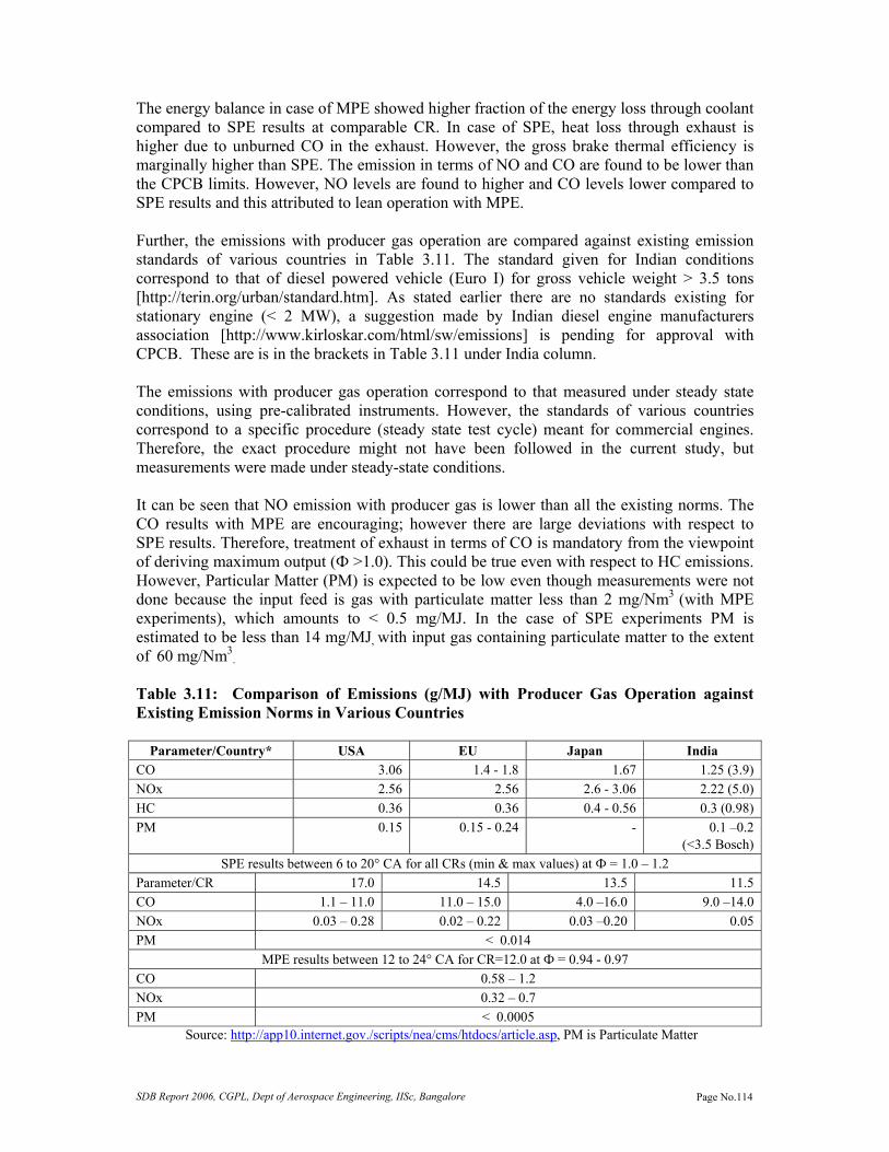
SDB Report 2006, CGPL, Dept of Aerospace Engineering, IISc, Bangalore Page No.114
The energy balance in case of MPE showed higher fraction of the energy loss through coolant compared to SPE results at comparable CR. In case of SPE, heat loss through exhaust is higher due to unburned CO in the exhaust. However, the gross brake thermal efficiency is marginally higher than SPE. The emission in terms of NO and CO are found to be lower than the CPCB limits. However, NO levels are found to higher and CO levels lower compared to SPE results and this attributed to lean operation with MPE. Further, the emissions with producer gas operation are compared against existing emission standards of various countries in Table 3.11. The standard given for Indian conditions correspond to that of diesel powered vehicle (Euro I) for gross vehicle weight > 3.5 tons [http://terin.org/urban/standard.htm]. As stated earlier there are no standards existing for stationary engine (< 2 MW), a suggestion made by Indian diesel engine manufacturers association [http://www.kirloskar.com/html/sw/emissions] is pending for approval with CPCB. These are is in the brackets in Table 3.11 under India column.
The emissions with producer gas operation correspond to that measured under steady state conditions, using pre-calibrated instruments. However, the standards of various countries correspond to a specific procedure (steady state test cycle) meant for commercial engines. Therefore, the exact procedure might not have been followed in the current study, but measurements were made under steady-state conditions. It can be seen that NO emission with producer gas is lower than all the existing norms. The CO results with MPE are encouraging; however there are large deviations with respect to SPE results. Therefore, treatment of exhaust in terms of CO is mandatory from the viewpoint of deriving maximum output (Ф >1.0). This could be true even with respect to HC emissions. However, Particular Matter (PM) is expected to be low even though measurements were not done because the input feed is gas with particulate matter less than 2 mg/Nm3 (with MPE experiments), which amounts to < 0.5 mg/MJ. In the case of SPE experiments PM is estimated to be less than 14 mg/MJ, with input gas containing particulate matter to the extent of 60 mg/Nm3
.
Table 3.11: Comparison of Emissions (g/MJ) with Producer Gas Operation against Existing Emission Norms in Various Countries
Parameter/Country* USA EU Japan India
CO 3.06 1.4 - 1.8 1.67 1.25 (3.9) NOx 2.56 2.56 2.6 - 3.06 2.22 (5.0) HC 0.36 0.36 0.4 - 0.56 0.3 (0.98) PM 0.15 0.15 - 0.24 - 0.1 –0.2
(<3.5 Bosch) SPE results between 6 to 20° CA for all CRs (min & max values) at Ф = 1.0 – 1.2
Parameter/CR 17.0 14.5 13.5 11.5 CO 1.1 – 11.0 11.0 – 15.0 4.0 –16.0 9.0 –14.0 NOx 0.03 – 0.28 0.02 – 0.22 0.03 –0.20 0.05 PM < 0.014
MPE results between 12 to 24° CA for CR=12.0 at Ф = 0.94 - 0.97 CO 0.58 – 1.2 NOx 0.32 – 0.7 PM < 0.0005
Source: http://app10.internet.gov./scripts/nea/cms/htdocs/article.asp, PM is Particulate Matter

SDB Report 2006, CGPL, Dept of Aerospace Engineering, IISc, Bangalore Page No.115
Observations Experimental studies have revealed engine operation to be smooth at a CR of 17.0 without any trace of knock thus establishing PG as a high-octane fuel. With the SPE engine, the extent of de-rating is observed to be 16.7% and 5% in terms of power and efficiency (gas to shaft power) respectively at the highest CR of 17 and it goes down to 27% and 21% respectively at CR of 11.5. The loss in power with PG operation is partly due to reduction in calorific value and partly due to reduction in the number of moles of the products released. In the case of MPE, the extent of de-rating is observed to be higher and the reasons for this feature are brought out. It is seen that the optimum ignition timing i.e MBT with producer gas operation more retarded when compared to gaseous fuels like natural gas (15° CA at 14.7 CR) with CH4 > 94% [Stone et al, 1996]. This is attributed to faster combustion due to laminar burning velocity being higher for producer gas compared to natural gas. Similarly MBT is retarded when compared with earlier works on producer gas and this is again attributed to producer gas constituents. Emission in terms of NO is observed to be lower partly due to lower peak cylinder temperature and partly due to MBT being retarded. However, CO emissions in the case of SPE are larger, which calls for slightly fuel-lean operations. Summary Experimental results pertaining to gas engine operations at two different power levels have been discussed. Important parameters like the MBT at different CRs for producer gas fuel have been brought out. Some of the engine pressure history data (p - θ curve) shall be compared against the zero-D predictions in Chapter VII.

SDB Report 2006, CGPL, Dept of Aerospace Engineering, IISc, Bangalore Page No.116
Chapter IV Zero-Dimensional Model Formulation This chapter discusses the formulation of zero-dimensional (0-D) model to simulate the SI engine cycle process. Eddy entrainment and laminar burn-up model based on flamelet concept of turbulent combustion are discussed. The parameters that need to be determined for using the above model are brought out. Introduction It is well recognized that the processes that govern the engine operation are extremely complex in nature. While much is known about these processes, there is no adequate understanding from the fundamental point of view. Therefore, it is difficult to make predictions of engine operation based on governing equations alone. Empirical relations and ad hoc approximations are being used to bridge this gap and these seem to be appropriate till better understanding prevails over the underlying physics. An advantage of such empirical models is that they can put to immediate use in areas of engine design and analysis. Therefore, thermodynamic or 0-D model still continues to be popular [Maly, 1994] among the engine designers because (i) what is of interest in many cases is the overall efficiency with power and (ii) it can be calibrated to appreciable accuracy by comparing against a wide set of experimental data on overall performance. They are also very useful in parametric studies of the effects of changes in engine operating variables on engine power and efficiency. Emissions can be captured only to a limited extent. These phenomenological models have been thoroughly discussed in the review paper by Blumberg et al [1979]. Sub-models of 0-D Model The zero-dimensional models are based on First Law of Thermodynamics, where time is the only independent variable. The model comprises of sub-models to simulate the processes of an engine cycle namely, intake, compression, heat release followed by expansion and exhaust. Depending upon the objective of the model, the sub-models are generally chosen. Since the objective of the present work is to simulate heat release, well-proven sub-model for turbulent combustion is chosen and relatively simpler sub-model is considered for the gas exchange process. However, pollutant formation is not modeled and heat transfer based on empirical relation is used. The various sub-models and empirical relation used in the present work are
• Filling and emptying technique (FET) for intake and exhaust processes as outlined by Heywood [1988].
• Eddy entrainment and laminar burn-up (EELB) model for simulation of heat release
as derived by Keck [1982]
• Heat loss due to convection based on Annand’s heat transfer correlations as discussed by Baruah [1986].

SDB Report 2006, CGPL, Dept of Aerospace Engineering, IISc, Bangalore Page No.117
Gas Exchange Process – FET Model In this model, the manifold is represented by finite volume where the mass of gas could increase or decrease with time. The mass and energy conservation equations coupled with mass flow rates into and out of the control volume – determined by equation of flow through a restriction are used to define the state of the gas in the control volume. The model also accounts for backflow of exhaust products into the intake manifold, but characterizes the contents of the manifold with a single gas temperature, pressure and composition. No wave action for charging during the intake and exhaust processes is accounted for. In this work, the engine is modeled as three open systems comprising of the intake system, the cylinder and the exhaust system. The FET has been proved to be an accurate tool [Heywood, 1988] for intake and exhaust processes for engines with small and compact manifold (ratio of exhaust system volume to displaced/swept volume ~ 1.2) by the earlier researchers [Janota et al, 1967]. Therefore, it has been taken appropriate to consider the above model for the present work since the engine that is being examined falls under such category (ratio of exhaust system volume to displaced/swept volume ~ 1.1). The output of this sub-model (in terms of pressure and temperature) serves as an initial condition for the subsequent in-cylinder process. Heat Release Process - EELB Model The concept of wrinkled flame or flamelet regime of turbulent pre-mixed combustion in a homogenous charged spark-ignition engine has been discussed in Chapter I. Based on these well conducted experimental investigations that include schlieren, shadowgraph and laser scattering measurements, an empirical equation for calculating burn rate, namely EELB has been derived by Keck [1982]. In this model, the flame propagation (or heat release) is modeled as a two-zone model, where a thin wrinkled multi-connected laminar flame separates the burned and the unburned mixture. The EELB model as formulated by Keck is represented in a pictorial form in Figure. 4.1
Figure 4.1: Schematic of Turbulent Premixed Spark-Ignition Engine Flame. Here uT is Characteristic Speed, lT is Characteristic Length Scale, SL is Laminar Burning Velocity, ρu is Unburned Gas Density and L is Reaction-Sheet/Flame Thickness, From Heywood [1988].

SDB Report 2006, CGPL, Dept of Aerospace Engineering, IISc, Bangalore Page No.118
It is mathematically stated in the form of two equations, namely
bLfu
b SAdt
dmτμ
ρ +=
(4.1)
bTfu uA
dtd
τμρμ
−=
(4.2)
where, parametric mass )( fTu AAl −= lρμ and characteristic time, b =lT/SL. Al and Af are laminar and spherical flame areas respectively. The relation between flame radius rf and burned gas radius rb based on experimental data is suggested by Keck [1982] as follows:
1→bf rr as 0→fr (4.3)
and ( ) bTbf urr τ→− as ∞→fr (4.4) An empirical equation, which satisfies these limiting conditions, has been suggested to be
( )( )( )2exp1 bTbbTbf ururr ττ −−+= (4.5)
Equation 4.1 represents the mass burn rate, the first term in this equation represents the laminar propagation of an approximately spherical flame front of the thick turbulent flame; the second term represents the burning of mixture already entrained with in this flame front. Equation 4.2 represents the rate of change of unburned mixture μ within the flame front, the first term represents the turbulent convection of unburned mixture across the spherical front of the flame and the second term represents the mass rate of burning of entrained but not-yet-burned mixture which is contained within the wrinkles and islands. This distortion and stretching of the thin reaction sheet is produced by the turbulent flow field [Heywood, 1988]. The four important validity limits identified [Keck, 1982] and Heywood [1988] for equation 4.1 and 4.2 are as follows:
• For a quiescent mixture, 0→Tu or ∞→Tl
LT SS ≅ (4.6) • Initially, as 0→t
LT SS → (4.7)
• Quasi-steady state, ,0≅dtdμ ,
LTT SuS +≈ (4.8) • Final burning after the flame front reaches the wall, wtt ≥ )0( →fA ,
{ }bwwbb tttmm τ/)(exp)(..
−−= -(4.9)

SDB Report 2006, CGPL, Dept of Aerospace Engineering, IISc, Bangalore Page No.119
Where, ST is the turbulent burning speed. Using the above formulation, Keck’s [1982] calculation of expansion speed (sum of turbulent burning speed and unburned gas speed) closely compares with the experimental results of Heywood et al [1984] for propane and hydrogen flame in an engine with simple geometry. It is reemphasized again here that Keck in his work [1982] brings out the need for validation of the above formulation for different geometrically shaped engines, especially those with significant swirl and squish. In these equations, there are two quantities, namely the characteristic speed and length, which could be related to the turbulence parameters namely turbulence intensity and length scale. Heywood [1988] relates the characteristic length scale to turbulent intensity u’ and characteristic length scale to Taylor length scale lM. It is also suggested that in order to use the above model, one needs to determine u’ and integral length scale lI, and subsequently lM could be determined with the assumption of homogenous and isotropic turbulence. These turbulence parameters can either be determined using empirical correlations or from fundamental studies. Keck [1982] has provided empirical relationship for obtaining characteristic speed and length by coupling with few other variables related to engine geometry. Similarly Borgnakke [1984] has suggested an empirical relation for estimating the value u’ at the start of combustion to the mean intake flow through the valve. Similarly, lI, at the start of combustion is considered to be proportional to a characteristic flow dimension, usually the clearance height. It further assumed that during combustion, the unburned mixture undergoes isentropic compression sufficiently rapidly that simple distortion process occurs. These are given as follows
( ) 3/10
'0
' ρρuu = ; ( ) 3/100,
' −= ρρII ll (4.10)
Where ρ refers to the density of the unburned gas and the suffix ‘0’ refers to the state to at the start of combustion. Some these correlations have been formulated for simpler geometries where turbulence is more dependent on the intake port design and less on the fluid-piston interaction inside the cylinder. Extending the same correlation is not appropriate for complex geometries where the flow is known to get substantially modified in the compression process. This leaves only with the other choice of estimating the turbulence parameters, namely by conducting a detailed 3-D modelling on the engine geometry under study. The computation of these turbulent parameters based on detailed CFD modelling is discussed in Chapter VI. The other important parameter set required to implement the EELB model is the laminar burning velocity for a particular fuel-air mixture, at thermodynamic conditions (pressure and temperature) encountered in an engine operation. The computation of laminar burning velocity for producer gas-air mixture is discussed in Chapter V. Heat Loss Modelling – Empirical Relation Convection is observed to be the dominant mode of heat transfer in SI engines [Heywood, 1988]. There are two sources for radiative heat transfer with in the engine cylinder: the high temperature burned gases and soot particles in the flame, if any. In a SI engine, the flame propagates across the combustion chamber from the ignition point through the previously mixed unburned mixture. Although the flame front is luminous, all the chemical intermediaries in the reaction process are gaseous and there is little scope for soot particles in the flame. However, in a compression- ignition engine, most of the fuel burns in a turbulent diffusion flame as the fuel drops vaporize and burn with air. The flame is reported to be highly luminous, and soot particles are formed as an intermediate step in the combustion

SDB Report 2006, CGPL, Dept of Aerospace Engineering, IISc, Bangalore Page No.120
process. Therefore the radiation from soot particles in the diesel engine flame is estimated about five times the radiation from the gaseous combustion products and accounts for about 20-35% of the total heat transfer and a higher fraction of maximum heat transfer rate. Since the present study is concerned with a SI engine, only convective mode of heat transfer is accounted in the 0-D model. Based on extensive experimental measurement over a wide range of engines empirical relations for heat transfer rate both in spark-ignition and compression ignition engines have been suggested by Annand [1963] and Woschni [1967]. The convective heat transfer flux from the gas to the cylinder wall given by Annand [1963] is as follows:
( ) )(Re.
wmb
w
TTDak
Aq
−= (4.11)
Where k is the thermal conductivity of the gas, Re is the Reynolds number based on mean piston speed and the characteristic dimension is the cylinder bore D, Aw is the effective combustion chamber area, Tm the mean temperature of the burned/unburned gas and Tw the wall temperature. a and b are constants. The value of a is expressed to vary between
8.035.0 ≥≤ a with the intensity of the charge motion and engine design and b = 0.7. In the present study, empirical relation of Annand [1963] is used in the 0-D model. A constant value of b=0.7 is chosen and for a, different values are chosen depending upon the process. This is essentially arrived at by calibrating the 0-D model against one of the experimental firing cycle with the heat transfer constant a tuned in such a way that heat loss to the walls and the exhaust match with the experimental values. The Reynolds number, Re is calculated on mean piston speed, which are 5.8 and 7.0 m/s corresponding to an engine speed of 1500 rev/min for LPE and MPE respectively. One important assumption considered in the 0-D model with respect to heat transfer is the constant wall temperature. Literature [French et al, 1973] indicates varying average wall temperature in the combustion chamber, with cylinder liner in the temperature range of 120 to 180° C and piston much higher based on measurements at various locations in a SI engine at CR = 8.5. A constant wall temperature of 450 K has been assumed for all the processes in the 0-D model. Modelling Details Making use of the sub-models as mentioned earlier, a full cycle thermodynamic model is constructed involving the following processes. Gas exchange process The 0-D calculations commence with the intake process of the (gas + air) mixture. Suitable discharge co-efficient is chosen for the intake and exhaust valve flow based on steady flow results on engines (with similar configuration valve) available in the Literature [Bicen et al, 1985]. The gas exchange period extends from the opening of exhaust valve to the closing of the inlet valve, when either one or both valves are open. The cylinder condition at the terminating point of the gas exchange period is called the trapped condition and this gives the thermodynamic initial condition for the subsequent in-cylinder processes. The cycle of events between the intake valve closing and the exhaust valve opening are (1) compression, (2) ignition delay and flame initiation (3) flame propagation and (4) expansion processes.

SDB Report 2006, CGPL, Dept of Aerospace Engineering, IISc, Bangalore Page No.121
Compression process The compression process commences with the closure of intake valve and compression of the trapped mass. The assumptions considered in this process are: perfect mixing model with the state of gas-air-recycled mixture being homogenous, chemical reactions being absent and pressure being uniform. At appropriate crank angle the ignition is initiated, following which is there is an apparent heat release delay. Using the first law of thermodynamics stated as
ααα ddVp
ddTmC
ddQ
v += (4.12)
and the equation of state of gas mRTpV = , the equations for pressure and temperature changes with respect to crank angle or time is obtained. These are expressed as
VddQ
CR
ddVp
CR
ddp
vv
11⎥⎥⎦
⎤
⎢⎢⎣
⎡⎟⎟⎠
⎞⎜⎜⎝
⎛+⎟⎟
⎠
⎞⎜⎜⎝
⎛+−=
ααα
(4.13)
and ⎥⎦
⎤⎢⎣
⎡+=
ααα pddp
VddVT
ddT
(4.14)
where, dQ is the heat loss obtained using equation 4.11. As the compression commences, the above variables are updated step-by-step using Euler’s method, given by the general expression given below, where Δα is the time step in crank angle.
)(*)()()( 1 αΔ+=+ nnn VariableVariableVariable (4.15) Flame Initiation and Ignition Delay Period The nominal ignition time is the instant when the spark occurs between the electrodes. However, there is a period of apparent delay between the time of sparking and the pressure rise due to combustion. It has been established by earlier researchers that flame propagates in a laminar mode till the flame kernel attains a critical size, beyond which the propagation becomes turbulent [Heywood 1988, Kalghatgi 1985]. In one case, Kalghatgi [1985] has identified the critical size of the flame to be around 11 mm radius for the propane and air gas mixture. This delay period is also considered as the time in which 1 to 10% of the initial unburned mass is consumed [Heywood, 1988]. Ignition delay is therefore considered to be the time required for the flame to assume a radius equivalent to 1% of the initial mixture by propagating at laminar burning velocity corresponding to the cylinder pressure and temperature. The estimated value is crosschecked by superimposing the computed motoring pressure-time curve with the experimental firing curve. In case of large differences between the two, the second method of estimation is considered. At the end of the ignition delay period, two physically distinct zones is considered to exist in the cylinder, one small part is formed by the flame kernel (at different pressure and temperature) and the rest by the unburned mixture. Further progress in computation is made by adopting the procedure, which identifies the steps for the two-zone calculations as discussed by Baruah [1986]. The procedure is of three steps, namely compression without combustion (Step I), during which

SDB Report 2006, CGPL, Dept of Aerospace Engineering, IISc, Bangalore Page No.122
the unburned mixture is considered to undergo normal compression process and this time period is same as the ignition delay period. The basis of this procedure is shown in Figure. 4.2.
m = mm 1 1 2mm 2mm
1Tm
T m 2Tm
p1p p2
V1V2
m ,T ,p ,Vp p p Heat loss dQm
2 2m T ,V , pp, p p 2
2 2V = V - Vm 2 p
T m
p
I II IIIInitial state Final Volume
Transform at fixed volume
Equalizationof pressure
//
//
/ /
/
// //
//
Figure. 4.2 Basis of Flame Initiation Process, From Barauh [1986] At the end the ignition delay period, there is a definite thermodynamic state for the unburned mixture, which is calculated on lines similar to that explained in the compression process. At this instant, Step II is considered, where in a flame kernel is assumed to appear instantaneously. This process is based on the assumption that flame nucleus is formed under constant volume conditions resulting in high pressure and temperature in the products region. With the combustion taking place at constant volume, the unburned mixture zone is maintained at constant temperature and pressure T’m and p’ respectively. The pressure, p” and temperature of products in the flame kernel, T”p are calculated from chemical equilibrium calculations, which are based on minimizing of Helmholtz energy. Similarly, the mass of the product is calculated corresponding to 1% of the trapped unburned mass. The total internal energy, E at the end of Step II is given by
ppmm ememE += (4.16) The assumption of constant volume combustion in the Step II produces a pressure difference between the unburned and burned zone. Since this is physically impossible, another step, namely Step III is required for pressure equalization. In this step it is assumed that pressure equalization occurs adiabatically and at constant volume, V2. This also implies the process is of constant internal energy, E. Flame Propagation At the completion of ignition delay period there are two distinct zones, separated by a flame front on which further computations are performed. A record is kept of the burned volume against the flame radius, and of the flame front area and flame contact with the cylinder wall and piston. With the advancement in calculations, the thermodynamic data pertaining to specific heats are accordingly updated based on the temperature in the burned and unburned zone. The principal assumptions made during this calculation are (1) the original charge is homogenous, (2) the pressure is uniform throughout the cylinder, (3) the volume occupied by the flame reaction zone is considered to be negligible, (4) the burned gas is at thermodynamic and chemical equilibrium, (5) the unburned gas is frozen at its original composition, (6) both burned and unburned gases have uniform local specific heats, (7) there is no heat transfer
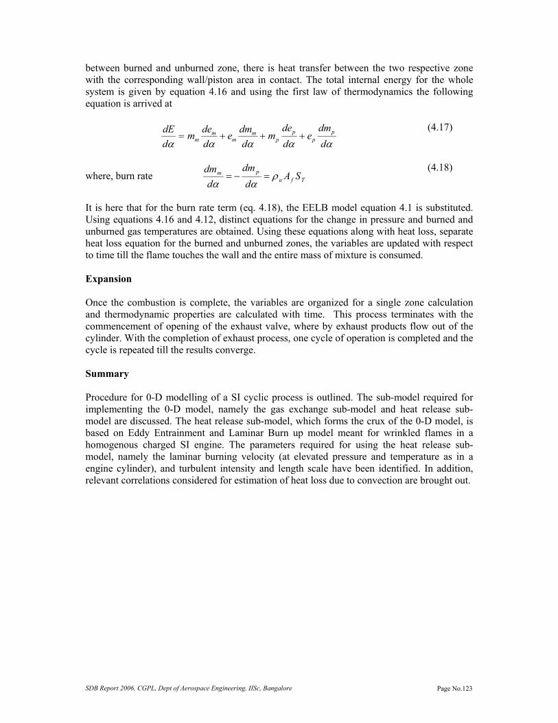
SDB Report 2006, CGPL, Dept of Aerospace Engineering, IISc, Bangalore Page No.123
between burned and unburned zone, there is heat transfer between the two respective zone with the corresponding wall/piston area in contact. The total internal energy for the whole system is given by equation 4.16 and using the first law of thermodynamics the following equation is arrived at
ααααα ddm
edde
mddme
ddem
ddE p
pp
pm
mm
m +++= (4.17)
where, burn rate Tfupm SA
ddm
ddm
ραα
=−= (4.18)
It is here that for the burn rate term (eq. 4.18), the EELB model equation 4.1 is substituted. Using equations 4.16 and 4.12, distinct equations for the change in pressure and burned and unburned gas temperatures are obtained. Using these equations along with heat loss, separate heat loss equation for the burned and unburned zones, the variables are updated with respect to time till the flame touches the wall and the entire mass of mixture is consumed. Expansion Once the combustion is complete, the variables are organized for a single zone calculation and thermodynamic properties are calculated with time. This process terminates with the commencement of opening of the exhaust valve, where by exhaust products flow out of the cylinder. With the completion of exhaust process, one cycle of operation is completed and the cycle is repeated till the results converge. Summary Procedure for 0-D modelling of a SI cyclic process is outlined. The sub-model required for implementing the 0-D model, namely the gas exchange sub-model and heat release sub-model are discussed. The heat release sub-model, which forms the crux of the 0-D model, is based on Eddy Entrainment and Laminar Burn up model meant for wrinkled flames in a homogenous charged SI engine. The parameters required for using the heat release sub-model, namely the laminar burning velocity (at elevated pressure and temperature as in a engine cylinder), and turbulent intensity and length scale have been identified. In addition, relevant correlations considered for estimation of heat loss due to convection are brought out.

SDB Report 2006, CGPL, Dept of Aerospace Engineering, IISc, Bangalore Page No.124
Chapter V Laminar Burning Velocity Calculations This chapter discusses the calculations of laminar burning velocity of producer gas + air + recycled gas mixture at pressures and temperatures typical of unburned mixture in a reciprocating engine. The effect of varying amount of recycled gas on the burning velocity is brought out. Based on a number of calculations at varying initial pressures and temperatures, and equivalence ratio, an expression for estimating the laminar burning velocity with the recycled gas mass fraction is obtained. Introduction Laminar burning velocity is the important intrinsic property of a combustible fuel, air and burned gas mixture. It is the velocity with which the flame propagates into a quiescent premixed unburned mixture ahead of the flame. The additional feature of engine related flame is the presence of residual or burned gas from the earlier cycle and this causes a reduction in the laminar burning velocity [Heywood, 1988]. The study of laminar burning velocity becomes relevant for estimating the burn rate in a spark ignition (SI) engine. Laminar burning velocities at pressure and temperature typical of a reciprocating engine operation are usually measured using spherical closed vessels. Data and derived correlations are available in the literature for a wide range of premixed air and fuel that includes hydrogen, methane, propane, iso-octane, methanol and gasoline [Heywood, 1988]. However, there have been a few studies using producer gas fuel, both computational and experimental (at ambient conditions) and some of these are highlighted here. In this chapter, procedure for computing of laminar burning velocity is discussed; subsequently the results of computations at thermodynamic conditions typical of a reciprocating engine along with a generalized correlation are brought out. Experimental - Earlier Studies Laminar burning velocity for producer gas - air mixture has been obtained by experiments and theoretical calculations for various compositions and mixture ratios by the earlier researchers [Kanitkar et al, 1993, Chakravarthy et al, 1993 and Mishra et al, 1994]. The laminar burning velocity at ambient conditions (0.92kPa, 300 K) has been experimentally determined by Kanitkar et al [1993] by conducting experiments using standard flame tube apparatus for producer gas - air mixture for a wide range of mixture ratios. These experiments were conducted at laboratory reference conditions using producer gas generated from an on-line IISc’s open top re-burn gasification system. The gas consisted of 18-23% H2, 17-20% CO, 3-4% CH4, 13-14% CO2 and rest N2. A wide range of mixture ratios were considered within the flammability limits of rich and lean mixtures, namely equivalence ratio (Φ) = 0.47 (26% fuel on volume basis) and 1.65 (56% fuel) for lean and rich limits respectively. The physical values of burning velocity varied between 0.10 to 0.13 m/s from lean to rich limits, with the peak value being 0.50+0.05 m/s around stoichiometry (45% fuel). The burning velocity for producer gas + air mixture is found to be higher by 30% compared to stoichiometric CH4 + air mixture at ambient conditions and with comparatively higher values at the lean limit (CH4 ~ 0.025m/s). This information is expected to help in understanding if the Minimum Advance for Best Torque (MBT) value for producer gas operation is
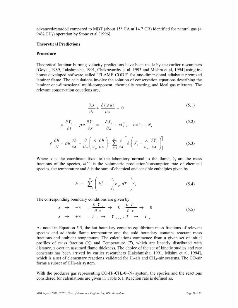
SDB Report 2006, CGPL, Dept of Aerospace Engineering, IISc, Bangalore Page No.125
advanced/retarded compared to MBT (about 15° CA at 14.7 CR) identified for natural gas (> 94% CH4) operation by Stone et al [1996]. Theoretical Predictions
Procedure Theoretical laminar burning velocity predictions have been made by the earlier researchers [Goyal, 1989, Lakshmisha, 1991, Chakravarthy et al, 1993 and Mishra et al, 1994] using in-house developed software called ‘FLAME CODE’ for one-dimensional adiabatic premixed laminar flame. The calculations involve the solution of conservation equations describing the laminar one-dimensional multi-component, chemically reacting, and ideal gas mixtures. The relevant conservation equations are,
0)(=
∂∂
+∂∂
xu
tρρ
(5.1)
,'''i
iii
xJ
xY
ut
Yωρρ &+
∂∂
−=∂∂
+∂∂
sNi ,,1K=
(5.2)
∑= ⎥
⎥⎦
⎤
⎢⎢⎣
⎡⎟⎟⎠
⎞⎜⎜⎝
⎛
∂∂
+∂∂
−⎟⎟⎠
⎞⎜⎜⎝
⎛
∂∂
∂∂
=∂∂
+∂∂ sN
i
i
pii
p xY
cJh
xxh
cxxhu
th
1
λλρρ
(5.3)
Where x is the coordinate fixed to the laboratory normal to the flame, Yi are the mass fractions of the species, ώ’’’ is the volumetric production/consumption rate of chemical species, the temperature and h is the sum of chemical and sensible enthalpies given by
h = i
N
i
T
Tpii YdTch
s
∑ ∫=
⎟⎟⎠
⎞⎜⎜⎝
⎛+
1
0
0
(5.4)
The corresponding boundary conditions are given by
uuii
i
TTYYxxT
xYx
→→+∞→
→∂∂
→∂∂
−∞→
,:
0,0:
,
(5.5)
As noted in Equation 5.5, the hot boundary contains equilibrium mass fractions of relevant species and adiabatic flame temperature and the cold boundary contains reactant mass fractions and ambient temperature. The calculations commence from a given set of initial profiles of mass fraction (Yi) and Temperature (T), which are linearly distributed with distance, x over an assumed flame thickness. The choice of the set of kinetic studies and rate constants has been arrived by earlier researchers [Lakshmisha, 1991, Mishra et al, 1994], which is a set of elementary reactions validated for H2-air and CH4–air systems. The CO-air forms a subset of CH4-air system. With the producer gas representing CO-H2-CH4-02-N2 system, the species and the reactions considered for calculations are given in Table 5.1. Reaction rate is defined as,

SDB Report 2006, CGPL, Dept of Aerospace Engineering, IISc, Bangalore Page No.126
jj
mRTE
fi CTeAdtdC ν∏=−
(5.6) where, Ci is the concentration of species and νj the stoichiometric coefficients of the reactions listed in Table 5.1. The values of frequency factor Af, activation energy E and coefficient m are given in Table 5.1. For each species, the NASA polynomial cure fits used to calculate the thermodynamic properties, namely specific heat, enthalpy and entropy. The transport properties such as diffusion coefficients and thermal conductivity for the mixture are evaluated using the correlations given in the report by Brokaw [1961]. The diffusive fluxes are calculated using the trace diffusion approximation neglecting the Soret and Dufour effects. The conservation equations are solved by finite difference scheme using operator-split technique. In this method the reaction equation is solved using an implicit method of the Crank-Nicholson type and the diffusion equation using the explicit forward-time central space (FTCS) scheme. The set of equations are solved at one time level and the properties at the next time level are obtained by a simple updating scheme. The burning velocities for different species are calculated and the convergence of these burning velocities as well with time of integration is used to determine the steady state. The results of burning velocity along with Yi and T constituted the output of the solution procedure.

SDB Report 2006, CGPL, Dept of Aerospace Engineering, IISc, Bangalore Page No.127
No. Reaction Af m E
R1 OH + O ↔ O2 + H 1.8E + 13 0.0 0.0
R2 O + H2 ↔ OH + H 1.5E + 07 2.0 76.58
R3 OH + H2 ↔ H2O + H 1.0E + 08 1.6 33.28
R4 OH + OH ↔ H2 + O 1.5E + 09 1.14 0.0
R5 H + H + M ↔ H2 + M* 9.7E + 16 -0.6 0.0
R6 H + OH + M ↔ H2O + M 2.2E + 22 -2.0 0.0
R7 O + O + M ↔ O2 + M 2.9E + 17 -1.0 0.0
R8 H + O2 + M ↔ HO2 + M 2.0E + 18 -0.8 0.0
R9 H + HO2 ↔ OH + OH 1.5E + 14 0.0 10.80
R10 H + HO2 ↔ H2 + O2 2.5E + 13 0.0 73.17
R11 O + HO2 ↔ OH + O2 2.0E + 13 0.0 0.0
R12 OH + HO2 ↔ H2O + O2 2.0E + 13 0.0 0.0
R13 HO2 + HO2 ↔ H2O2 + O2 2.0E + 12 0.0 0.0
R14 OH + OH + M ↔ H2O2 + M 3.3E + 22 -2.0 0.0
R15 H + H2O2 ↔ H2 + HO2 1.7E + 12 0.0 37.4
R16 H + H2O2 ↔ H2O + OH 1.0E + 13 0.0 36.1
R17 O + H2O2 ↔ OH + HO2 2.8E + 13 0.0 64.35
R18 OH + H2O2 ↔ H2O + HO2 7.0E + 12 0.0 14.03
R19 CO + H + M ↔ CHO + M 6.9E + 14 0.0 17.0
R20 CO + O + M ↔ CO2 + M 7.1E + 13 0.0 -45.11
R21 CO + OH ↔ CO2 + H 4.4E + 07 1.5 -74.1
R22 CO + HO2 ↔ CO2 + O 1.5E + 14 0.0 24.0
R23 CO + O2 ↔ CO2 + O 2.5E + 12 0.0 48.15
R24 CH4 + H ↔ CH3 + H2 2.2E + 04 3.0 87.61
R25 CH4 + O ↔ CH3 + OH 1.2E + 07 2.10 76.28
R26 CH4 + OH ↔ CH3 + H2O 1.6E + 06 2.10 24.76
R27 CH4 + M ↔ CH3 + H + M 5.7E + 17 0.0 92.24
R28 CH3 + O ↔ CH2O + H 7.0E + 13 0.0 0.0
R29 CH3 + O2 ↔ CH2O + O 1.5E + 13 0.0 29.7
R30 CH2O + H ↔ CHO + H2 2.5E + 13 0.0 40.40
R31 CH2O + O ↔ CHO + OH 3.5E + 13 0.0 35.38
R32 CH2O + OH ↔ CHO + H2O 3.0E + 13 0.0 12.03
R33 CH2O + CH2 ↔ CHO + CH4 1.0E + 11 0.0 61.64
R34 CH2O + M ↔ CHO + H + M 1.4E + 17 0.0 76.85
R35 CH2O + M ↔ CO + H2 + M 2.0E + 16 0.0 38.0
R36 CHO + H ↔ CO + H2 2.0E + 14 0.0 0.0
R37 CHO + O ↔ CO + OH 3.0E + 13 0.0 0.0
R38 CHO + O ↔ CO2 + H 3.0E + 13 0.0 0.0
R39 CHO + OH ↔ CO + H2O 5.0E + 13 0.0 0.0
R40 CHO + O2 ↔ CO + HO2 3.0E + 12 0.0 0.0

SDB Report 2006, CGPL, Dept of Aerospace Engineering, IISc, Bangalore Page No.128
* M represents the third body, which is chaperon efficiency weighed total concentration Table 5.1: Kinetic Scheme Used for the Present Laminar Burning Velocity Calculations [Warnatz,
1984]. Af in cm3.s mole, E in kcal/moleThe burning velocity is calculated from
iLS , = s
biuiu
i
NiYY
dx,......,2,1,
)( ,,
'''
=−
∫+∞
∞−
ρ
ω&
(5.7)
TLS , = )(
1
'''
buu
Ns
i
o
ii
HH
dxh−
∫ ∑+∞
∞− =
ρ
ω&
(5.8)
where, Hu and Hb is the total enthalpy of the unburned mixture and burned gases respectively.
Predictions – High Pressure In one of the earlier studies [Chakravarthy et al, 1993] conducted using the above code for producer gas+ air mixture at ambient conditions, the theoretical predictions compared well within the error band of experimental data. In one of the subsequent studies [Mishra et al, 1994], predictions at higher pressures indicated the burning velocity of producer gas to reduce from 0.4 m/s at 1 atm (300 K) to 0.04 m/s at 40 atm (300 K). Such a drastic reduction in burning velocity at high pressure was attributed to the drastic reduction in the radical pool due to suppression of dissociation. This drastic reduction in burning velocity at higher pressure has relevance in the field of internal combustion engine because of similar pressures encountered during operation. However, this effect can be expected to be completely modified by the corresponding increase in temperature on account of compression in a reciprocating engine. Current Work – High Pressure and Temperature Along with Recycled Gas The zero–dimensional calculations required input in the form of laminar burning velocity at pressure and temperature prevalent in the engine cylinder at the time of initiation of ignition. Therefore, producer gas + air mixture compositions comparing closely with the experimental data at varying mixture ratios were considered. In an actual reciprocating engine operation, there is some amount of burned product that is trapped in the clearance volume from the previous cycle, as also there is some amount of the reverse flow of burned products from the cylinder into the intake manifold.
Manifold pressure, mmHg abs
Rec
ycle
d ga
s fra
ctio
n, %
Figure. 5.1 A Trace of Recycled Gas (RG) Variation with CR Recorded on a SI Engine
at 1400 rev/min [see Heywood, 1988]

SDB Report 2006, CGPL, Dept of Aerospace Engineering, IISc, Bangalore Page No.129
The extent or fraction of recycled gas in the fresh mixture depends upon the compression ratio (CR) and the valve overlap period. The data on recycled mass fraction from literature [see Heywood, 1988] as a function of CR is shown in Figure. 5.2. In order to simulate the mixture conditions close to an actual SI engine operation, varying amounts of recycled gas fraction (0 to 10%) are considered for the calculations and these are well within the recycled gas mass fraction for engines with CR between 17 and 11.5:1. The fuel considered is of nominal composition with 20 % each of H2 and CO, 2% CH4, 12% CO2 and rest N2. Calculations are made at varying equivalence ratio (Φ), initial temperature and pressure and with varying amounts of recycled gas 0, 5 and 10%. The results of these computation are shown in Table-5.1 for two identified producer gas + air mixture and at two equivalence ratios.
Table 5.2: Computational Laminar Burning Velocity at Varying Initial Conditions of Mixture – Pressure, Temperature and Recycled Gas (RG) Mass Fraction.
Pressure, bar (abs)
unburnedT , K
LS , cm/sec Case I* Case II# Φ =0.90 Φ =1.07 Φ =0.90
0% RG
0% RG
5% RG
10% RG
0% RG
5% RG
10% RG
5 630 105 143 130 112 122 110 92
10 746 132 179 162 139 154 144 113
15 821 151 205 183 159 176 151 132
20 876 163 217 196 169 189 166 141
25 920 173 229 205 176 200 174 148
30 954 178 236 207 180 206 180 152
35 995 191 249 213 186 221 190 164
40 1028 202 259 231 189 227 198 176
45 1056 207 268 238 200 235 208 181
50 1082 215 275 245 204 243 214 190 * Case I Corresponds to H2 = 20%, CO= 18%, CH4 =2%, CO2 = 12% and rest, N2
# Case II Corresponds to H2 = 20%, CO= 20%, CH4 =2%, CO2 = 12% and rest, N2 Recycled Gas for Case I and II is H2O =12%, CO2 =15% and rest, N2
It is clear from the above data that burning velocities decrease substantially with dilution at all initial mixture pressure conditions and Φ. This essentially occurs due to reduction in the adiabatic flame temperature due to dilution. The effect of dilution on the burning velocity is shown in Figure 5.2 for rich and lean fuel +air mixture at different initial mixture pressures. The proportional reduction in laminar burning velocity is essentially independent of the unburned mixture equivalence ratio, initial pressure and temperature over the range of computation conducted. This effect is consistent with studies conducted by Rhodes et al [1985] using gasoline fuel at initial pressure of 1 and 2 atmospheres.

SDB Report 2006, CGPL, Dept of Aerospace Engineering, IISc, Bangalore Page No.130
A least-square curve fitting done using the data of Case II resulted in an expression for laminar burning velocity in terms of cylinder pressure and is as follows.
LS (cm/s) = 94.352744.0
0⎟⎟⎠
⎞⎜⎜⎝
⎛pp ( )( )( )ψ4.2112.196.0 −−Φ+
(5.9)
0.6
0.7
0.8
0.9
1
0 2 4 6 8 10 12RG mass fraction, %
Rat
io o
f SL(R
G) t
o S L
(0) P Φ
5 0.90
20 0.90
40 0.90
5 1.07
20 1.07
40 1.07
Figure 5.2: Effect of Variation of Recycled Gas (RG) on the Laminar Burning Velocity at Rich and Lean Mixtures and Different Initial Pressures.
where, p is the cylinder pressure in bar (abs), po the reference pressure (1.0 bar), Ψ the recycled gas mass fraction and Φ the fuel-air equivalence ratio. The burning velocity dependence upon the initial temperature is built into the pressure term in Equation 5.8. The above correlation is correct within + 6% for the data of Case II. This correlation fits for the data in Case I by including a correction factor due to lower CO content, which is explained below. It has been brought out in Chapter III that laminar burning velocity for producer gas is about 30 % higher than natural gas at ambient conditions. The burning velocity of producer gas is quite sensitive to the variations in fraction of H2 and CO and this is quite possible in the process of gasification. A sensitivity analysis of variation in CO and H2 content towards laminar burning velocity at a equivalence ratio of about 0.9 revealed the burning velocity to reduce by about 7% for reduction of every 1% in H2 or CO content. To further explore the behaviour seen above, the heat lease rate is examined at six varying conditions. The conditions examined correspond to 40 and 20 bar (abs) initial pressure with 0, 5 and 10% recycled gas fraction. The two pressures listed above are the typical working pressure at the highest and lowest CR dealt in this thesis. The heat release rate across the flame is plotted as a function of non-dimensional temperature for six conditions in Figure. 5.3. The initial unburned gas temperature and the corresponding adiabatic flame/burned gas temperatures are given in Table 5.3. It is very much evident from the plot the influence of RG on the heat release rate at both initial mixture pressures.

SDB Report 2006, CGPL, Dept of Aerospace Engineering, IISc, Bangalore Page No.131
0.E+00
6.E+05
1.E+06
2.E+06
0 0.1 0.2 0.3 0.4 0.5 0.6 0.7 0.8 0.9 1
Hea
t Rel
ease
Rat
e, M
W/c
m3 40 bar, 0% RG
)/()( ubu TTTT −−=τ
40 bar, 5% RG
40 bar, 10% RG
20 bar with 0% RG 20 bar, 5% RG
20 bar, 10%
4.2
2.5
8.4
0.0
Figure 5.3: Heat Release Rate Profile vs. Non-Dimensional Temperature across the Flame at Two Initial Mixture Pressure of 20 and 40 bar (abs), with and without Recycled Gas (RG). Table 5.3: Laminar Burning Velocity and Laminar Flame Thickness at Φ =1.07 for Different
Pressures and Recycled Gas (RG)
Pressure 20 bar (abs) 40 bar (abs) RG, % 0 5 10 0 5 10
uT , K 876 876 876 1028 1028 1028
bT , K 2330 2275 2200 2450 2395 2345
LS , cm/s 217 196 169 259 231 189
Lδ , mm 0.23 0.21 0.19 0.092 0.13 0.09 The distance between positions of 1% (initial temperature, Tu) and 99% (adiabatic flame/burned gas temperature, Tad or Tb) temperature rise is used for the estimation of the flame thickness, δL and is shown in Table 5.3. The δL is about 0.21 + 0.02 mm and 0.1 + 0.01 mm at 20 and 40 bar (abs) pressure respectively. The order of flame thickness is well within the values measured experimentally by Smith [1982] ~ 0.2 mm for propane fuel under engine conditions. Similarly, the flame thickness according to the procedure of Abraham et al [1985], (ratio of thermal diffusivity to laminar burning velocity) works out about 0.8 microns. The kolmogorov length scale, lk for the engine under study is about 4 microns (for a ReT =2100 and lI =1.2 mm, assuming isotropic and homogenous turbulence: lk = lI ReT -3/4). Therefore, the ratio of lk/δL ≈ 5.0 implying flame can be treated as negligibly thin in the context of wrinkled flame structure relevant to SI engine [Abraham et al, 1985]. Summary A correlation for estimation of laminar burning velocity as a function of initial pressure and recycled gas fraction is obtained. This expression is used in the 0-D model to estimate the burn rate for a wide range of operating conditions.

SDB Report 2006, CGPL, Dept of Aerospace Engineering, IISc, Bangalore Page No.132
Chapter VI CFD Modelling This chapter discusses the detailed three-dimensional modelling of a reciprocating engine geometry comprising of a flat cylinder head and a bowl-in-piston combustion chamber, simulating the motoring or non-firing conditions. The turbulence is modelled using standard
ε−k model and the results are compared against experimental results from the literature. Relevant turbulence parameters and velocities extracted from the modelling study are used in the 0-D model whose predictions are discussed in the next chapter. Introduction Turbulence in reciprocating engines is considered important because of its large influence on the combustion characteristics. In order to find optimum conditions in a combustion system, it is essential to get a good approximation of the in-cylinder turbulence. From this viewpoint, multi-dimensional modelling using CFD codes is pursued and involves simulation with and without combustion. One of the major challenges of CFD in the recent times is that several models need to be combined in order to simulate a complete engine cycle. The ε−k model is the most commonly used turbulence model in CFD, even though its deficiencies are known [Versteeg et al, 1995], indeed ε−k model is still considered to the best compromise between computational time and precision. However, in the recent times, second-moment closure models are being pursued in engine modelling [Lebrere et al, 1996; Watkins et al, 1996], with the increased validity of the model. But complex numerical approaches such as Direct Numerical Simulation (DNS) are difficult to implement on engine like situation, because of enormous pre-requisites such as high mesh density and exorbitant CPU time. This is also the case with Large Eddy Simulation (LES), where accurate sub-grid models are required, and research in this field is still in progress [Lebrere et al, 1996]. For implementing CFD model, mesh density assumes primary importance; some of the earlier studies on engine geometry using different mesh densities are summarized in Table 6.1. From the above Table 6.1, it is evident that the computational mesh densities have increased with the enhancement in the computational speed over the period of two decades. Reasonably good qualitative (a few cases quantitative) comparison have been claimed by the some of the researchers listed above with mesh density less than 0.12 million cells, by using turbulence models such as ε−k in most cases and second order closure model in one case [Lebrere et al, 1996]. They claim the grid independent solution based on global balances in momentum and kinetic energy, with mesh refinement to have little effect on the results. In the present work, a detailed 3-D cold flow study is conducted on piston-engine geometry with a mesh density of 0.2 million cells to simulate the engine cold flow condition. CFD simulation is conducted over two complete motoring cycles involving intake, compression, and expansion and exhaust processes on a bowl-in piston engine geometry at two CRs, namely 17.0 and 11.5. Data on the turbulence parameters, and reverse squish velocities (referred as the reverse squish period during the beginning of expansion process) derived from the above study are used as input in the 0-D modelling. Similarly, a hypothetical path for the flame kernel movement is obtained from the CFD results. This is estimated by tracking the velocity of a particle along a streak line, in and around the point of ignition. The simulation is conducted using a commercial CFD code CFX - 4.3. The grid is generated using

SDB Report 2006, CGPL, Dept of Aerospace Engineering, IISc, Bangalore Page No.133
a pre-processor called CFX-build. The numerical solution is obtained using CFX-solver, which is based on finite volume technique. The results are analysed using a post-processor known as CFX-Analyse.
Table 6.1: CFD Studies on Engine Geometries with Different Mesh Densities
Researcher Summary of The Work Geometry & Mesh Schapertons et al [1986]
Cold flow studies in two different bowl-in piston geometries of a diesel engine
Engine cylinder, 0.02 million cells
Haworth et al [1990]
Cold flow studies with different intake valves and limited comparison with experimental results.
Intake pipe and engine cylinder, 0.023 million cells
Trigui et al [1994]
Cold flow studies using STAR-CD code; experimental flow field data used as initial conditions.
Engine cylinder, 0.06 million cells
Jones et al [1995]
Cold flow in a four valve pent roof SI engine through two complete cycles using SPEED code. Predictions compared qualitatively and quantitatively (one case) with the experimental results.
Engine cylinder, 0.03 million cells
Strauss et al [1995]
Simulation of combustion in a indirect combustion chamber geometry of diesel engine using SPEED code
Engine cylinder, 0.0425 million cells
Reuss et al [1995]
Cold flow studies compared against Particle Image Velocimetry results using KIVA and GMTEC code
Engine cylinder, 0.06 million cells
Khalighi et al [1995]
Flow and combustion modelling in a four-valve SI engine. Cold flow results compared with water-analog flow studies. Numerical inaccuracies discussed.
Engine cylinder, 0.023 - 0.12 million cells
Lebrere et al [1996]
Cold flow using ε−k and second-order closure turbulence model. Predictions compared against LDA measurements.
Engine cylinder, 0.072 million cells
Bauer et al [1996]
Flow through intake system of a SI engine using STAR-CD code. Predictions of instantaneous pressure and temperature in the intake system compared with the experimental results.
Intake system and engine cylinder, 0.12 million cells
Duclos et al [1996]
Simulation of SI engine combustion using KIVA – II code and compared with the experimental results.
Intake pipe and engine cylinder, 0.12 million cells
Problem Definition The geometry considered for modelling is identical to the combustion chamber geometry of Small Power level Engine (SPE). The combustion chamber comprises of a flat cylinder head and an eccentrically located hemispherical bowl. The geometric details of the engine are given in Table 3.1. The piston, which is one of the moving boundaries, simulates the reciprocating movement of an engine. The minimum clearance between the piston and the cylinder head as the piston approaches its uppermost point of travel is about 1.5 mm for a CR of 17.0 and increases to 5.2 mm at CR of 11.5. The other moving boundary is formed by the intake valve (non-swirl type) to allow fluid flow into the cylinder geometry. The geometry is also provided with an exhaust port that is opened at appropriate time to simulate the exhaust process. Since the simulation does not involve combustion, simplifying the geometry with a port in place of a moving exhaust valve is taken not to influence the accuracy of the results. The geometry described above is relatively complex, involving a time dependent grid to simulate the piston and intake valve movement. This is achieved by writing additional fortran programmes to simulate the transient grid in the present study. Simulation is also conducted

SDB Report 2006, CGPL, Dept of Aerospace Engineering, IISc, Bangalore Page No.134
on a flat piston (without the bowl) at a CR=17.0 in order to assess the magnification of turbulence intensity caused by the presence of bowl. Grid Generation The geometry described in Cartesian co-ordinate system is required to simulate the reciprocating engine operation. This is achieved using a multi-block grid methodology, in which a set of unstructured blocks is glued together, and on each of them is a structured grid. In the resulting geometry with a three-block structure, it is found that there is a mismatch of the grids at the interfacing planes. These are resolved by identifying the interfacing nodes of the adjacent blocks as ‘unmatched’ and thereby allow the solver to adopt appropriate methodology for data transfer between the adjacent blocks. Also suitable regions are identified as ’patches’ in order to define the boundary conditions. The type of grid adopted for this geometry is ‘two-way bias’. In this approach, the grid density increases from the central region towards the walls. The
(i) (ii)
Figure 6.1: Grid Distribution (i) with the Intake Valve Fully Closed and Piston at TC (ii) with Intake Valve Fully Open and Piston at BC. The Physical Dimensions of the Geometry are: a=116 mm, b=110 mm diameter, c=60 mm diameter, d=30 mm and e=1.5/5.2 mm for CR=17.0/11.5 Respectively. grid distribution with the piston at extreme positions is shown in Figure. 6.1. When the piston is at BC, the minimum and maximum grid sizes are 0.01 mm and 3.0 mm in the axial direction and 3.5 mm in the radial direction and azimuthal spacing about 4.0 degree. Similarly, when the piston is at TC, the change in the grid size occurs only in the axial direction and corresponds to a minimum and maximum of 0.01 mm and 0.03 mm respectively. This grid pattern corresponds to a mesh density of 0.2 million computational nodes. The geometry is created with the piston at TC and the intake valve fully closed as
Grid Size: Cyl. region
Max: 3 x 3.5 x 3.8 mm
Grid Size: Bowl Region
Max: 2 x 1 x 0.6 mm
Grid Size: Y axis
0.01 – 0.03 mm
a
c
b
e
d

SDB Report 2006, CGPL, Dept of Aerospace Engineering, IISc, Bangalore Page No.135
shown in Figure 6.1 (i). Further, the intake and the piston move in accordance to the engine cycle operation to simulate different processes. Boundary and Initial Conditions
0
2
4
6
8
10
12
420 520 620 720 820 920
Crank Angle, degrees
Val
ve L
ift, m
m
Valve OverLap period
Intake ValveExit Valve
Figure 6.2 Valve- Lift Profile of the Engine (SPE)
Figure 6.3 Schematic Diagram of the Evolving Fluid Flow during Intake, Compression and Early Part of Expansion in a Bowl-In Piston Engine Geometry. The Central Figure Shows the Tangential Velocity Plot in the Circumferential Plane, 1.2 mm below the Intake Valve. The Axial View Corresponds to the Velocities along Section –DD. ‘S’ denotes Separation Zone and ’T’ denotes Tumbling Vortices. 360° CA Corresponds to TC and 250° CA Flow After Intake Valve Closure.
The flow domain considered for simulation is downstream of the engine intake manifold. Therefore, flow through intake manifold is not modelled. However, the transient flow condition in the intake manifold is accounted by introducing time-varying boundary condition (pressure) at the intake valve. The manifold pressure profile is generated from the actual pressure measurements on the experimental engine (SPE). These are obtained using a strain gauge transducer mounted on the intake manifold, very close (upstream) to the intake valve of the cylinder, with the engine operating at rated speed (1500 rev/min). Similarly, intake valve movement is simulated using the actual valve lift profile of the engine as shown in Figure. 6.2. In the computations, a minor change in the intake valve opening timing is introduced in order to simply the grid movement. The intake valve opens at TC instead of actually opening a few degrees (26° CA) earlier. Similarly, the closure of the exhaust port occurs at TC. The valve overlap period is thus not simulated and it is anticipated not to effect the predictions since the simulation does not involve combustion. The complete closure of the intake valve is simulated by making the grid size at the valve region to low value (< 0.25 mm) and imposing wall condition subsequently. The computations commence with the induction process in which a set of initial conditions is assumed for the first cycle. Initial conditions for some of the variables are obtained from motored 0-D results, namely, initial pressure and temperature. The initial conditions correspond to a pressure of 920 kpa (corresponding to atmospheric pressure at Bangalore) and a temperature of 300 K for the working fluid (air). However suitable assumptions are made of the remaining variables. The three components of velocity are taken as 0.001 m/s; similarly, initial low values for turbulence kinetic energy and dissipation rate are assumed at

SDB Report 2006, CGPL, Dept of Aerospace Engineering, IISc, Bangalore Page No.136
0.001 m2/s2 and 0.001 m2/s3 respectively. A constant wall temperature of 450 K is considered through out the simulation. The working fluid is treated as a single gas since combustion is not considered. These computations are repeated over two complete cycles in order to obtain results independent of the initial conditions. Aspects of Modelling The CFD code solves the 3-D, ensemble-averaged Navier-Stokes and enthalpy equations governing turbulent and compressible gas flow along with heat transfer for the geometry described above. To simulate the turbulence parameters, standard ε−k model has been chosen without and with compressibility effects due to velocity dilatation. The working fluid is treated as a single gas since combustion is not simulated. The algorithm employed for spatial and temporal discretisation is 1st order accurate hybrid and backward difference schemes respectively. The governing equation set includes the continuity equation, three momentum equations, the enthalpy equation and two turbulence equations. For flow calculations with a moving grid, the transport equations are suitably modified [Hawkins et al, 1991]. There are two main changes: the transient term allows for the change in volume and the advection terms include the grid velocity. The complete sets of equations are as follows:
0))(.(1=
∂∂
−∇+∂
∂txU
tg
gρ
ρ
(6.1)
σρρ
.))(.(1∇+=⊗
∂∂
−∇+∂
∂BU
txU
tUg
g
(6.2)
tx
tpTH
txU
tHg
g ∂∂
∇−∂∂
=∇∇−∂∂
−∇+∂
∂.).())(.(1 ρλρ
ρ
(6.3)
where, g accounts for the expansion and compression of the grid, x is the grid position, U is the velocity, H is the total enthalpy, B is the body force, λ is the thermal conductivity and σ the stress tensor. Similar transformation is applied for the turbulent transport equations. The transport equations for turbulence kinetic energy, k and turbulence dissipation rate, ε are as follows: The equation for k is given by
ρεσμμρρ
−=∇+∇−∇+∂∂ PkUk
tk
k
T )).(().( (6.4)
Where, P is the shear production defined as,
).(.32))(.( kUUUUUP eff
Teff ρμμ +∇∇−∇+∇∇=
(6.5)
The equation for ε without compressibility effect is given by

SDB Report 2006, CGPL, Dept of Aerospace Engineering, IISc, Bangalore Page No.137
kCP
kCU
tT
2
21)).(().( ερεεσμμερρε
ε
−=∇+∇−∇+∂∂
(6.6)
The equation for ε with compressibility effect is given by
UCk
CPk
CUt
T .)).(().( 3
2
21 ∇+−=∇+∇−∇+∂∂ ρεερεε
σμ
μερρε
ε
(6.7)
where, μ is molecular viscosity, μT the turbulence viscosity and σ the Prandtl number. The values of constants are C1 = 1.44, C2 = 1.92, C3 = - 0.373. The constants C1 and C2 are the standard constants used in ε−k model. The value considered for C3 is same as that of Jennings [1992]. Since the flow is considered compressible, the equation of state is the ideal gas law given by
RTP ρ= (6.8) Numerical Scheme The numerical scheme of CFX solver is based on finite volume technique, and involves the following steps
• Integration of the governing equations of fluid flow over all the control volumes of the solution domain.
• Discretisation involves substitution of the terms in the integrated equation
representing flow processes such as convection, diffusion and sources with finite-difference type approximation and thereby converting into algebraic equations. In the present modelling, the algorithm employed for spatial discretisation is hybrid scheme and is 1st order accurate. Similarly, a 1st order accurate backward difference scheme is employed for temporal discretisation.
• Solution of the algebraic equations is obtained by an iterative method.
Computational Procedure Computations have been made for an operational speed of 1500 rev/min, with time step of the order of 0.5° CA (50 micro seconds). The calculations commence with the piston at TC, with the intake valve and exhaust port closed. Using the initial and boundary conditions as mentioned earlier, the computation proceeds with the piston descending downwards and the intake valve beginning to open so as to allow fluid to enter the flow domain i.e. cylinder. The closure of the intake valve (the passage between the valve and cylinder head is reduced to less than 0.25 mm) takes place in accordance with the actual valve timing of the engine. The intake valve closes at 64° ABC (After Bottom Centre), at which time the boundary condition at the intake valve is changed from ‘pressure’ to ‘wall’ to prevent fluid escaping from the cylinder. The valve closure is halted with a cell size of less than 0.25 mm to prevent collapse of the grid. In this transitional period a lower time-step of the order of 0.01° CA (1 micro second) is adopted to so as to prevent divergence in the solution. Further upward movement

SDB Report 2006, CGPL, Dept of Aerospace Engineering, IISc, Bangalore Page No.138
of the piston results in compression of the fluid till the piston reaches TC, beyond which fluid expansion occurs. The exhaust port opens at 38° BBC (Before Bottom Centre) by introducing a pressure boundary condition at the exhaust port. The exhaust process continues till the piston reaches TC, which completes one cycle of operation. Using the results of the first cycle as the initial condition, the second cycle is computed. This procedure is repeated to simulate operations at two CRs namely, 17 and 11.5. On the flat piston geometry computations are attempted at CR = 17. Calculations are done with a grid density of 0.2 million cells. For a time step of 0.5° CA, the number of iterations employed to get converged solution is about 70. The time step independence of the calculations has been verified. The principal results extracted from these calculations are velocities at the intended location of spark plug and turbulence parameters namely, turbulence intensity, u’ and integral length scale, lI. CFD Results It is clear from the current experimental investigations that optimum ignition timing for producer gas fuel is close to TC. At this particular setting, the major part of the combustion occurs during reverse squish regime, it was thought prudent to focus the CFD results in the later part of the compression (around the time of piston approaching TC) and early part of expansion process (retreating from TC). Heywood [1988] indicates to the induction system and the piston geometry having significant effect on the in-cylinder flow characteristics. The initial in-cylinder flow pattern set up during the induction process is observed to modify in the subsequent process in a few geometries, as also observed in the present study. In this section, schematic diagram derived from the velocity profile across selected plane is discussed. Further, two-dimensional velocity vectors and contour plot of scalar variable at time intervals close to TC are presented. The flow field related to bowl-in piston geometry is mainly discussed, and at important juncture, the result of flat piston geometry is brought out in order to highlight the features of geometry under investigation. Turbulence intensity is calculated using the correlation - Turbulent Kinetic Energy = 3/2 u’ 2 Velocity Distribution The flow during the induction is observed to be transient, highly turbulent and fluctuating. The evolving flow pattern as a function of time is schematically shown in Figure. 6.3, these are derived from the velocity profiles across the axial plane passing through the centre of the geometry, the schematic shown in the circumferential plane is in below the cylinder head (1.2 mm), in the plane of intake valve opening. The flow field is observed to be as follows. During the initial stages of suction process, there are two major rotating flow patterns established in the cylinder as a consequence intake jet interacting with the walls of the cylinder. One flow pattern is termed as swirl (rotating mass about the cylinder axis) and occurs as the flow is discharged tangentially towards the cylinder wall, where it is deflected sideways and downward in a swirling motion. The other flow pattern occupying major part of the domain is observed in the transverse direction and is termed as tumble (rotating mass normal to the cylinder axis). Apart from these, there are recirculating flows in local regions in the vicinity of cylinder head/bore interface and these occur due to flow separation. These are evident from Figure 6.3 (at 30° CA) that shows the separation of the jet at the intake port and setting up of strong re-circulating pattern at the corner of the geometry and also the commencement of tumbling flow vortices. The tumble flow is constituted by two-barrel type vortices, which are observed to be asymmetric against symmetric vortices observed by Ekchian et al [1979] in water-analogy experiments.

SDB Report 2006, CGPL, Dept of Aerospace Engineering, IISc, Bangalore Page No.139
This difference in the flow pattern is due to off-axis valve location in the current case against axisymmetric in-flow with Ekchian et al [1979]. The flow pattern in the case of off-axis valve is much more complex even though a similar structure is observed and this is due to uneven flow distribution over the intake port cross section. The flow pattern at 60° CA corresponds to the piston approaching the maximum instantaneous speed. There are two vortices visible with different centres of rotation. The vortex away from the wall (right side) is rotating in the clockwise direction, with the center of rotation close to the top of piston. The second vortex is close to the wall (left side) and rotating in the counter-clockwise direction, with the center of rotation at a higher plane beneath the intake port. In addition, there is distinct flow pattern visible in the bowl region. These vortices are continually convected with the fluid as evident from the location of centre of rotation of the left vortex corresponding to a piston position at 120° CA. It is also evident that the sense of rotation of the right side vortex is reversed and is same as the left side vortex. These vortices further disintegrate and merge into a single vortex by the time the piston reaches the bottom centre (BC) – 180° CA. Further, during ascendance of the piston in the compression process, single vortex in the cylindrical region is visible after the closure of the intake valve corresponding to 250° CA. The intensity of the swirling and the tumbling motion are normally quantified in terms of swirl and tumble ratio. These are defined as follows:
Swirl ratio = NMH yy π260 and Tumble ratio = NMH zxzx ,, 260 π Where Hx,, y, ,z and M x,, y, ,z is the angular momentum and moment of inertia about x, y, z axis respectively and N is the speed of the engine in rev/min. These ratios change with the evolving flow pattern and are shown in Table 6.2 at particular crank angles. Tumble ratio is specified in x and z planes about the instantaneous fluid center of rotation where as swirl ratio is computed about the y-axis of the geometry or bowl axis. The swirl ratio is quantified at regular time intervals, however the tumble ratio is quantified in the event of single tumble present in the flow domain and this only occurs in the last stages of intake and early part of compression process.
Table 6.2: Computed Parameters at Specific Crank Angles
° CA Swirl Ratio* (Y-axis)
Swirl Ratio+ (Bowl-axis)
Tumble Ratio (X-axis)
Tumble Ratio (Z-axis)
180 1.00 1.60 1.35 1.35 250 0.85 1.41 1.50 1.50 270 0.90 1.45 1.40 1.40 300 0.82 1.63 1.20 1.20 330 0.50 1.10 NC NC 360 0.30 0.40 NC NC
* Complete Domain, + Bowl Region, NC: Not Calculated – Regime of Two Tumble As the piston ascends upwards during the compression process, the fluid from the cylindrical region is pushed into the bowl region thereby increasing the angular velocity of the fluid in the bowl. The fluid flow pattern till the commencement of later part of compression process

SDB Report 2006, CGPL, Dept of Aerospace Engineering, IISc, Bangalore Page No.140
is found to be same for both CRs. However, as the piston approaches TC (> 330° CA), the squish effects fluid movement into the bowl and the squish velocities are found to be vastly different with either CRs. Due to the squish effect (becomes dominant); the fluid in the cylindrical portion is pushed into the bowl leading to formation of two vortices in the bowl. The peak squish effect is observed to occur around 350° CA, shown in Figure. 6.4, where in the local velocities are as high as 20 m/s around the edge of the bowl corresponding to CR=17. There is a slight asymmetry in the velocity distribution probably due to eccentricity of the bowl. The velocity vector plot in the axial plane at the same crank angle shows the evolution of counter rotating toroidal vortices. At TC (360° CA) the counter-rotating vortices continue to survive and get displaced downwards in the bowl. These results are qualitatively compared with some of the experimental observations of Arcoumanis et al [1983]. These researchers have experimentally measured the mean and turbulence velocities on an axi-symmetric engine of CR = 6.7 at a speed of 200 rev/min using three piston geometries, which include the bowl-in piston geometry under motoring conditions.
20 m/s
TT
10 m/s
Section - DD
21 m/s
C
C
B
D D
B Speed along the Dotted Line
Figure 6.4: Vector Plot in the Axial Plane (Section –DD) during Squish Period Corresponding to 350° CA – CR=17.0. Vector Plot in the Circumferential Plane is at a Distance of 1.2 mm below Cylinder Head, the Dotted Circle in Circumferential View Represents the Edge of the Bowl.

SDB Report 2006, CGPL, Dept of Aerospace Engineering, IISc, Bangalore Page No.141
Measurements are reported to have been done in the presence and absence of swirl so as to access its influence on the mean and turbulence velocities. The results from the Arcoumanis et al [1983] are compared with the CFD results in Figure. 6.5. The predicted flow field pattern compares favourably (in the sense of vortex rotation) with the experimental results observed in the absence of intake swirl. However, CFD result shows the existence of swirl during intake (peak swirl ratio ~ 2.1 @ 50° CA) process. Further comparison with the experimental flow field in the presence of intake swirl (opposite sense of rotation of vortex, shown as Figure 6.5v) would not appropriate because the mean piston speed in either case is widely different (experiments is 0.63 m/s against 5.8 m/s in CFD) and with squish velocity being linearly dependent on piston speed [Heywood, 1988], it is conjectured that the behaviour would be vastly different in either case.
Figure 6.5: (i) Vector Plot in the Circumferential Plane is at a Distance of 1.2 mm below the Cylinder Head corresponding to 360° CA (TC) –CR=17.0, (ii) Speed along the Dotted Line, (iii) Velocity in the Axial Plane –Section DD, (iv) and (v) Experimental Results about the Symmetry Plane from Arcoumanis et al [1983] at 360° CA (TC) in the Absence and Presence of Intake Swirl Respectively. Dotted Circle Represents the Edge of the Bowl.
Speed along the Dotted Line
TT
8 m/s
Section -DD
8 m/s
10 m/s
B
C
DD
C
B
(i)
(iv) (v)
(iii)
(ii)

SDB Report 2006, CGPL, Dept of Aerospace Engineering, IISc, Bangalore Page No.142
The swirl ratio at the end of the compression process is quantified as 0.3; this reduction in swirl could be due to interaction of swirl with the squish. Further, as the piston descends downwards from TC the effect of reverse squish sets in where the fluid begins to flow out of the bowl into the cylindrical region and in the process the counter-rotating vortices are displaced upwards. Here, it is necessary to emphasize that reverse squish effect is vastly different with either CRs and these are brought out later in this section. The fluid movement further intensifies with the piston descending downwards as shown in Figure. 6.6, maximum reverse squish effect becomes evident at about 370-372° CA, where in the velocities are as high as 31 m/s with asymmetry in velocity distribution.
8 m/s
(iii)
(ii)(i)
(iv)
(v)
TT
Distance (mm)
Spee
d (m
/s)
0.210
25
1.25 2.5
Section - DD
28 m/s
B
B
D
C
C Speed along the Dotted Line
Figure 6.6: (i) Vector Plot in the Circumferential Plane at a Distance of 1.2 mm below the Cylinder Head corresponding to 370° CA – CR=17.0, (ii) Speed along the Dotted Line, (iii) Velocity in the Axial Plane –Section DD, (iv) Enlarged View of the Velocity Plot Near the Edge of the Bowl and (V) Speed in the Axial Direction – along the Dotted Line Shown in (iv). Dotted Circle Represents the Edge of the Bowl.
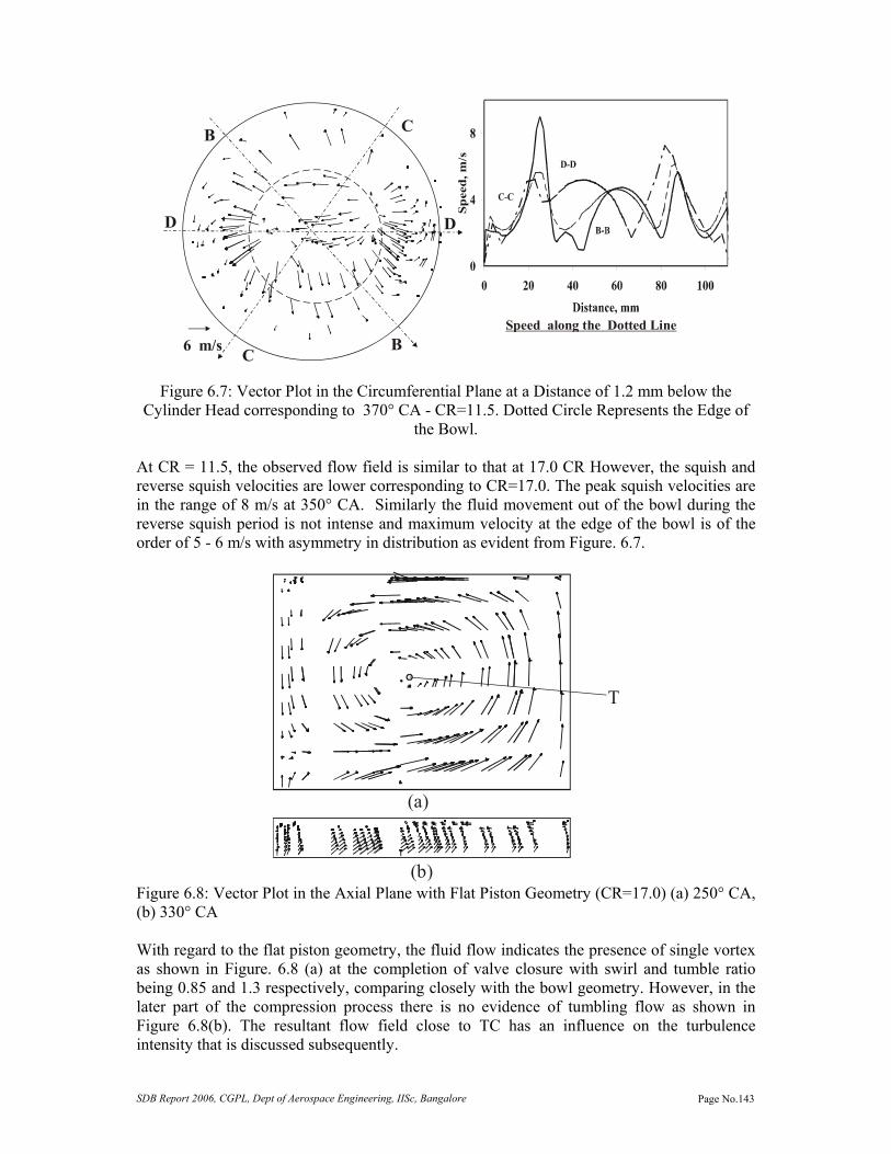
SDB Report 2006, CGPL, Dept of Aerospace Engineering, IISc, Bangalore Page No.143
C
C
DD
B
B6 m/sSpeed along the Dotted Line
Figure 6.7: Vector Plot in the Circumferential Plane at a Distance of 1.2 mm below the Cylinder Head corresponding to 370° CA - CR=11.5. Dotted Circle Represents the Edge of
the Bowl. At CR = 11.5, the observed flow field is similar to that at 17.0 CR However, the squish and reverse squish velocities are lower corresponding to CR=17.0. The peak squish velocities are in the range of 8 m/s at 350° CA. Similarly the fluid movement out of the bowl during the reverse squish period is not intense and maximum velocity at the edge of the bowl is of the order of 5 - 6 m/s with asymmetry in distribution as evident from Figure. 6.7.
(a)
T
(b) Figure 6.8: Vector Plot in the Axial Plane with Flat Piston Geometry (CR=17.0) (a) 250° CA, (b) 330° CA With regard to the flat piston geometry, the fluid flow indicates the presence of single vortex as shown in Figure. 6.8 (a) at the completion of valve closure with swirl and tumble ratio being 0.85 and 1.3 respectively, comparing closely with the bowl geometry. However, in the later part of the compression process there is no evidence of tumbling flow as shown in Figure 6.8(b). The resultant flow field close to TC has an influence on the turbulence intensity that is discussed subsequently.

SDB Report 2006, CGPL, Dept of Aerospace Engineering, IISc, Bangalore Page No.144
Summarizing the flow field results, the jet-like character of the intake flow interacting with the cylinder walls and the moving piston, creates large scale rotating flow pattern within the cylinder. The flow field is observed to undergo large-scale changes during intake and subsequently in the compression process. Between the two CRs with bowl-in piston geometry, it is observed that there is no distinct change in the fluid flow pattern in the intake and early part of the compression process. However, in the last stages of compression and early part of expansion, the fluid velocities near the edge of the bowl are largely different, the high CR creating large shear zones near to the edge of the bowl. Between the flat head and bowl-in-piston geometries, the swirl and tumble ratio are about the same during intake process. During compression the swirl ratio is found to be higher in the bowl region due to increase in the angular velocity of the fluid. However, there is one distinct difference observed between the two geometries, in the case of bowl-in piston geometries there is evidence of formation of two tumbling vortices and these survive till TC. In the flat piston geometry, there is evidence of a single tumbling vortex during early part of the compression and is dissipated much earlier to the completion of compression process. The effect of this flow pattern on the turbulence generation is discussed subsequently. Turbulence Distribution The variation in turbulence intensity (u’) and integral length scale (lI) is firstly discussed. Further insight is provided by examining the spatial distribution of turbulence kinetic energy in and around TC, which is relevant from the combustion viewpoint. Figure 6.9 shows the CFD results of u’ values for the bowl-in piston geometry in the diametric plane (4 mm below the cylinder head). The computed results are shown with and without the compressibility effects in the ε - equation. Examination of the computed results reveals large variation in u’ right through the induction and compression process. Initial high turbulence is set in due to shear in the high velocity jet entering the cylinder. The turbulence fluctuation, u’ goes to as high as 22 m/s and this approximately coincides with the point of maximum piston speed and the valve lift, further to which there is fall in turbulence intensity with commencement of intake valve closure. The turbulence fluctuation, u’ again increases post beyond intake valve closure due to increased fluid movement and peaks at about 30° CA prior to TC, subsequent to which there is decline. These results are comparable with and without accounting for the compressibility effect in the ε- equation. Further, the results are compared with the experimental results of Catania et al [1996] as shown in Figure 6.9. These experiments are conducted on a production diesel engine of CR = 18.0, with slightly re-entrant bowl-in piston geometry using hot-wire anemometer at varying speed ranging between 600-3000 rev/min. The comparison is made considering the results at two engine speeds, namely 1500 and 2000 rev/min, which corresponds to two mean piston speeds of 4.3 and 5.8 m/s. The comparison of the u’ between the two results appears fair (considering the fact that the geometries are similar, but not identical) till about inlet valve closure. In this time period, the location of the peak value is different by about 30 to 40° CA and this is attributed to differences in intake valve timing/valve lift profile. Beyond the intake valve closure one finds opposing trends in the variation of u’ with CA. As the piston starts compressing the fluid, there is an increase in u’ and peaks at 30° BTC beyond which there is a decline in u’ against continuous decline in the measured values. In the post - TC region, there is again a contradictory trend in comparison to experimental results. This feature is unaltered even when compressibility effect is accounted by choosing a constant of -0.373

SDB Report 2006, CGPL, Dept of Aerospace Engineering, IISc, Bangalore Page No.145
[Jennings, 1992] for the velocity dilatation term in the ε-equation. In the work of Han et al [1995], using RNG ε−k model on Mexican hat piston top where the effect of velocity dilatation and kinematic viscosity are accounted in the ε equation, similar qualitative behaviour of u’ declining in the post-TC period as noted here has been observed. Similarly, other experimental studies in the literature suggest the trend of increase in u’ for certain bowl-in piston geometries, namely the re-entrant configuration compared to simpler cylindrical configuration in the post-TC period [Corcione et al, 1994] and this is inferred as due to higher shear zones with re-entrant geometries.
Figure 6.9: Top Plot is the CFD Result Using k-ε Model (with and without Compressibility Effect) as a Function of Crank Angle. ref is the Experimental Result of Catania et al [1996] on a Similar Configuration Engine. The Bottom Plot (solid line) shows the Variation of Instantaneous Piston Speed Normalized with the Mean Piston Speed (5.8 m/s) – for the CFD Geometry and Corresponding to 2000 rev/min of ref. The Dotted Line is the Intake Valve Lift Profile of the CFD Geometry. Maximum Intake Valve Lift for ref is 8.1 mm. Next the mass-averaged u’ and lI as a function of CR are shown in Figure. 6.10, the location corresponds to mid 3-D zone in the bowl region of the geometry. It is clear from the figure that variation of u’ with time is close to being independent of CR; these are consistent with the observations made by Lancaster [1976] and Ikegami et al [1987]. Similarly, the variation of lI calculated using k and ε are also shown in Figure. 6.10, which indicates lI to be higher at lower CR compared to higher CR and is qualitatively consistent with the experimental results of Ikegami et al [1987].
0
5
10
15
20
25
Tur
bule
nce
Inte
nsity
,u' (m
/s)
TC
2000 rev/min [ref ]
Std k-ε model
1500 rev/min [ref ]
k-ε Model with Compressibility Effect
IVC (ref )
0
369
12
0 75 150 225 300 375Crank Angle (Degree)
Lift
(mm
)
-2
0
2
Sp'/S
p

SDB Report 2006, CGPL, Dept of Aerospace Engineering, IISc, Bangalore Page No.146
Figure 6.11 shows the comparison of u’ for both the piston geometries. The variation in u’ with time is about the same until early part of the compression process. In the later part of the compression process, it is evident that decline in u’ is faster in the case of the flat geometry. This declining behaviour could be due to following reasons (i) absence of squish generating mechanism with flat geometry (ii) absence of tumbling vortices in the later part of compression process. The absence of turbulence generating mechanism like squish in the case of flat geometry is evident. However, it is important to recognize the role of the tumbling vortices taking note of the literature. Floch et al [1995] have studied the influence of swirl and tumble on the turbulence intensity and combustion in a SI engine. Their study indicates the breakdown of the tumbling vortices (prior to TC) to be responsible for enhancement of turbulence along with decline in the tangential velocities. It is conjectured that tumble contributes to higher turbulence due to the dissociation of the main vortex into turbulence as a result of piston movement. It is further observed that in the case of swirl, the rotating motion is conserved during compression process thereby contributing to turbulence generation to a lesser extent (due to lesser swirl dissociation). Similarly Urushihara et al [1995] observe that tumble flow generates turbulence in combustion chamber more effectively than swirl flow does, and that swirling motion reduces the cycle-by-cycle variation of mean velocity which tends to be generated by the tumbling motion. In the current study, there is evidence of tumble vortex breakdown with flat piston geometry much earlier to TC, this apart from the absence of squish appears to be responsible for the faster decline in u’.
0
2
4
6
8
10
330 340 350 360 370 380Crank Angle (Degree)
Tur
bule
nce
Inte
nsity
, u' (m
/s)
0
1
2
3
4
5
6
Inte
gral
leng
th sc
ale,
l I (m
m)
CR 17.0
CR
TC
Mass-Averaging Zone
~ 15 mm thick
Figure 6.10: Variation of Mass Averaged u’ and lI across a 3D Zone Shown in the Inset at
Varying CRs.

SDB Report 2006, CGPL, Dept of Aerospace Engineering, IISc, Bangalore Page No.147
0
5
10
15
20
25
0 75 150 225 300 375Crank Angle (Degree)
Turb
ulen
ce In
tens
ity (m
/s)
TC
Bowl-in-Piston
Flat Piston
Figure 6.11: Comparison of u’ for the Two Piston Geometries – 4 mm below Cylinder Head.
Next, the spatial distribution of turbulence kinetic energy (TKE) at crank angles close to TC and for both CR and for the flat piston geometry is shown in Figure. 6.12. The contour plots in the axial plane reveal spatial variation in TKE and this is consistent with the experimental observations of Schapertons et al [1986]. A general observation at all time steps indicates the TKE to be of high intensity in the central region of the bowl decreasing towards the walls. Another revealing information from the contour plot is the shifting in the distribution of TKE with time and this is caused due to changes in the flow pattern occurring in the bowl region due to squish and reverse squish effects. It is also observed that the TKE is marginally lower (5%) at higher CR probably due to enhanced dissipation of kinetic energy on account of increased fluid movement during squish and reverse squish period. Lastly, the comparison of TKE of the two-piston geometries reveals substantial enhanced TKE for bowl-in piston geometry compared to the flat piston. In case of flat geometry, the turbulence kinetic energy is more or less uniform through out the combustion chamber.

SDB Report 2006, CGPL, Dept of Aerospace Engineering, IISc, Bangalore Page No.148
322142
43
3225
350° CA
350° CA
350° CA
360° CA
360° CA
360° CA
370° CA
( a )
370° CA ( b )
370° CA ( c )
Figure 6.12: CFD results: Contour Plot of Turbulence Kinetic Energy (m2/s2) on an Axial Plane Through the Centre of the Geometry (a) Bowl Geometry – CR = 17.0 (b) Bowl Geometry – CR = 11.5 (c) Flat Geometry – CR = 17. Other Inputs for the 0-D Model Other than the turbulence parameters, the velocity (normal component) in the region of the ignition source (spark plug) is required in order to allow for the possible flame movement during the process of ignition delay and subsequent flame propagation. This data is extracted from the CFD data by plotting streak line. A streak line is drawn for a zero mass particle originating at a point near to the ignition source into the bowl region and it is shown in the inset of Figure. 6.12. The normal component of velocity obtained at location nearest to the streak line is considered for flame displacement/movement and is shown in Figure. 6.13 for both CRs 17.0 and 11.5. It is evident from the plot that there is flow reversal due to reverse squish effect (in the path of streak line) subsequent to TC in the case of CR=17.0 and not so with CR=11.5 (in the path of streak line) due to lower reverse squish velocities. These velocities are considered for flame displacement in the 0-D model.
422856
314661
223445
3523
832
24
24
15
17

SDB Report 2006, CGPL, Dept of Aerospace Engineering, IISc, Bangalore Page No.149
Other than the turbulence parameters, the velocity in the region of the ignition source (spark plug) is required in order to consider for the possible flame movement during the process of ignition delay and subsequent flame propagation. The existence of higher squish/reverse squish velocities in the case of higher CR is evident from Figure 6.14, which shows velocities at the edge of bowl in the time period around TC. It is not so in the case of lower CR. The CFD data is further compared with the values obtained from correlation discussed by Heywood [1988]. It must be brought out that the squish velocities obtained from the correlation are in the absence of combustion and without effects like gas inertia, friction, gas leakage past piston rings and heat transfer. The predicted velocities from CFD qualitatively match with the correlation data, with some real time effect like heat transfer included in the simulation the CFD results are considered appropriate as an input for the 0-D model.
-7
-6
-5
-4
-3
-2
-1
0
1
2
320 330 340 350 360 370 380 390
Crank Angle, degree
Vel
ocity
, m/s
TC
CR=17.0
CR=11.5
Reverse Squish
Squish
Streak line
Figure 6.13: Normal Component of Velocity along a Streak Line from the Point of Ignition at
Two CRs from CFD Studies
-40
-30
-20
-10
0
10
20
30
40
300 325 350 375 400 425
Crank Angle, degree
Vel
ocity
, m/s
CFD @ 11.5CFD @ 17.0COR @ 12.0 COR @ 17.0COR @ 11.5
Reverse squish
Squish TC
Figure 6.14: Comparison of Squish and Reverse Squish Velocities from CFD and using an Empirical Correlation –COR [Heywood, 1988] for SPE Geometry (CR=17.0 and 11.5) and MPE Geometry (CR=12.0).

SDB Report 2006, CGPL, Dept of Aerospace Engineering, IISc, Bangalore Page No.150
Observations 3-D computations on engine geometry are able to capture the generic features of fluid flow in a reciprocating engine and are consistent with some of the experimental observations available in the literature. The presence of high shear zones near to the edge of the bowl during squish/reverse squish is evident, more so in the case of higher CR with bowl-in piston geometry. The standard ε−k model predicts trends in TKE in and around TC different from experiments and this is reasoned to be due to limitation of the ε−k model to capture transient effects due to squish/reverse squish phenomenon. The difference in the fluid flow pattern compared bowl-in piston during the later part of the compression process appears to the cause for u’ to be lower in the case of flat piston geometry. Summary Three important results have been extracted from the motored 3-D computations to be used in 0-D model to predict p-θ curves and these are (i) mass-averaged turbulence parameters, namely turbulence intensity and integral length scale, (ii) velocity (normal component) for flame kernel movement/displacement, (iii) extent of velocities near to the edge of the bowl in the reverse squish regime.

SDB Report 2006, CGPL, Dept of Aerospace Engineering, IISc, Bangalore Page No.151
Chapter VII Predictions of Zero-D Model This chapter discusses the Zero-D (0-D) predictions, where in the pressure-crank angle curves are predicted on two engine geometries at different compression ratios. Full cycle thermodynamic analysis is dealt with both engine geometries. Introduction The basis of this chapter is the thermodynamic model that has been described in Chapter IV. The heat release that forms the primary part of the model is based on eddy entrainment and laminar burn-up models. Two important parameters have been identified to implement this model. One of these is the laminar burning velocity at pressures and temperatures typical of unburned mixture in a reciprocating engine; this has been numerically computed as brought out in Chapter V. The other parameter set is related to turbulence characteristics and fluid velocities at the time of ignition and subsequent flame propagation. These have been quantitatively derived from the CFD analysis conducted on the SPE geometry and since the combustion chamber of MPE also involves a bowl-in-piston, the results of SPE geometry are extended to the MPE geometry for 0-D predictions. Using these data, the heat release part of the engine cyclic process is predicted, prior to which the initial thermodynamic conditions are established using the gas exchange sub-model. For the heat release sub-model, the details of the combustion chamber geometry with respect the shape and size of the bowl and the location of the spark plug are considered. 0-D predictions are attempted on the combustion chamber geometry of SPE at varying CR and ignition advance; similarly predictions are attempted at a fixed CR at two ignition settings for the MPE geometry. The energy balance results obtained from the full-thermodynamic cycle are further compared with the experimental results. Engine Combustion Chamber Geometry Small Power level Engine
Bowl radius 30 mm
Piston
Spark plug
Exitvalve
Intakevalve
Edge of bowl
X X
Section - XX
Figure 7.1: Combustion Chamber of SPE

SDB Report 2006, CGPL, Dept of Aerospace Engineering, IISc, Bangalore Page No.152
The combustion chamber comprises of a flat cylinder head and hemispherical shaped bowl as shown in Figure. 7.1. The bowl is eccentrically located on the piston top with a shift of about 3 mm from the axis. The bowl measures 30 mm in radius, with a volume of 55 + 1 cc. The flat portion of the piston top provides a squish ratio of 0.7 with respect to the cylinder head. The bumping clearance between the cylinder head and flat portion of the piston measures 1.5, 3.4 and 5.2 mm at 17.0, 13.5 and 11.5 CR respectively. The spark plug is located close to center (offset of 8 mm from the axis of the cylinder), with the spark plug electrode flush with cylinder head. There is one intake valve and one exit valve of directed type measuring 39 and 33 mm diameter respectively to allow flow into and out of the cylinder. The valve has a maximum lift of 11 mm as shown in the Figure 6.2 of Chapter VI. Medium Power level Engine
Spark plug
Edge of bowl
Exitvalve
Intakevalve
Bowl radius 36.5 mmHeight:31.3 mm
Piston
X X
Section - XX
Figure 7.2: Combustion Chamber of MPE In this case, the combustion chamber is formed of the flat cylinder head and a centrally located cylindrical shaped bowl as shown in Figure 7.2. The bowl measures 73 mm in diameter and 31.3 mm in height with a volume of 131 cc. The squish ratio is about 0.68 with a minimum bumping clearance of 1.6 mm. There is also additional volume in the form of small depression on the piston top for valve accommodation. However, in this geometry, the spark plug is not centrally located but placed at a point, which is close to the outer edge of the cylindrical bowl and could have additional influence on the flame kernel movement. The chamber is provided with one intake and exit valve of directed type measuring 46 mm diameter with a maximum lift of 14 mm with opening and closure in accordance to the valve-lift profile as shown in the Figure 7.3.

SDB Report 2006, CGPL, Dept of Aerospace Engineering, IISc, Bangalore Page No.153
0
2
4
6
8
10
12
14
16
420 520 620 720 820 920
Crank Angle, degrees
Val
ve L
ift, m
m
Valve OverLap period
Intake ValveExit Valve
Figure 7.3: Valve-Lift Profile of MPE
Validation of Motoring Curve Prior to proceeding with the prediction of firing p-θ curves, computations under motoring conditions are validated by comparing with the in-cylinder motoring curve recorded on the engines. The experimental motoring curve is recorded on an engine operating under wide-open throttle condition and with the engine operating at the rated speed. p-θ curve is recorded by conducting a “grab” motoring test where the instrumented cylinder of the engine is switched rapidly from firing to motored operation as outlined by Heywood [1988]. This is achieved by cutting-off the spark to the instrumented cylinder and subsequently recording the pressure history. The data used in 0-D simulation is shown in Table 7.1. An important outcome of this motoring simulation is the estimation of charge trapped inside the cylinder at the closure of the intake valve, along with an estimation of recycled gas mass fraction at the beginning of a fresh cycle. In order to arrive at these conditions, it is required to properly account for the charge-flow into and out of the cylinder by choosing appropriate values for discharge coefficients (Cd) for the intake and exit valves. For the present work, values of Cd, of 0.32 and 0.55 are chosen for the intake and exit valves respectively. Cd value chosen for the exit valve is consistent with the steady flow studies quoted in the literature [Bicen et al, 1985], whereas Cd for the intake valve is lower (around 0.5 quoted in the literature) and this is assumed because of additional pressure drop upstream of the intake manifold (200 mm of water against 30 - 40 mm in diesel mode of operation) caused due to long passage from the gas source. The valve lift profiles have been appropriately considered along with the valve overlap period as shown in Figs. 6.2 and 7.3. The pressure variations in the intake and the exit manifold are also a part of the simulation, and therefore a constant boundary condition is chosen upstream and downstream of intake (90 kPa and 300 K) and exit manifold (92 kPa and 300 K). Heat transfer is neglected for the manifold part of the flow.

SDB Report 2006, CGPL, Dept of Aerospace Engineering, IISc, Bangalore Page No.154
Table 7.1: Data for 0-D Simulation
Wall Temperature 450 K Simulation Speed 1500 rev/min Annand Coefficient for Heat Transfer - a
Suction Compression & Expansion Exhaust 0.2 0.8 0.4 Annand Coefficient for Heat Transfer - b 0.78
Recycled Gas Mass Fraction (%) with CR 17.0 CR 13.5 CR 11.5 CR 12.0 CR 6.5 7.5 8.5 8.5 Boundary Condition Intake Manifold 90 kPa and 300 K Exit Manifold 92 kPa and 300 K Cd, - Intake and Exit valve 0.32 and 0.55
However, for the in-cylinder computations Annand’s heat transfer correlation [Annand et al, 1963] is used with varying heat transfer co-efficient as shown in Table 7.1 (values for ‘a’ in Eq. 4.11 discussed in Chapter IV). The above coefficients are established by trial-and-error procedure using one test case corresponding to an ignition advance of 26° CA at CR = 17.0. 0-D cycle predictions are made by tuning the above coefficients till the predicted overall energy balance approximately match with the corresponding experimental data. The value chosen for the compression process is higher due to the engine geometry [Annand et al, 1963]. In fact the values chosen for the suction and compression process match with the heat transfer data obtained the cold-flow CFD studies. For the expansion and exhaust processes of the firing cycle, the values for the coefficient are chosen in accordance with the information available in the literature [Annand et al, 1963]. A constant wall temperature of 450 K has been chosen throughout the analysis. The motored pressure history is simulated using producer gas and air mixture and validated against the experimental p-θ curve in order to arrive at the realistic initial thermodynamic conditions. This validation procedure is followed for SPE at all CRs. The possible error in pressure matching is well within 0.5% for all the cases. However, for the MPE, validation could be possible at a slightly different operating condition (at lower intake charge pressure), because of difficulty in getting experimental motoring curve at corresponding operating condition. During experimentation it was observed that cutting off spark to one cylinder lowered the engine output and thereby affected the turbo-charger performance in terms of charge pressure to the cylinders. Therefore validation is done with the experimental motoring curve at charge pressure of 1.1 bar (abs) and the required thermodynamic conditions corresponding to higher brake output is obtained by changing the charge pressure in the intake manifold (1.25 bar at a gross brake output of 160 kW). Assumptions and Features for the 0-D Model The assumptions and features for the 0-D model are listed below
• The gas exchange process is simulated Filling and Emptying technique. The details are discussed in section 4.2.1 of Chapter IV. The intake and exit boundary conditions, and Cd for the valves are given in Table 7.1.

SDB Report 2006, CGPL, Dept of Aerospace Engineering, IISc, Bangalore Page No.155
• All the four processes, namely gas exchange, compression, heat release and expansion are simulated with heat loss, and mixture/product gas considered as perfect gas. The heat transfer coefficients used for different processes are listed in Table 7.1. A constant wall temperature of 450 K is considered for all processes.
• Subsequent to ignition occurring a preset time, there is an apparent time delay in
cylinder pressure rise due to combustion called the ignition delay. During the ignition delay period the flame kernel is displaced from its point of formation.
• The combustion is considered to occur under constant volume conditions, with
products and mixture at different pressures. At the end of ignition delay period the pressure in the combustion chamber equilibrates in accordance to the procedure discussed in section 4.3.3 of Chapter IV.
• With further movement of the flame, the heat release is simulated using EELB sub-
model as outlined in section 4.2.2, wherein a spherical flame front (reaction zone) is assumed to propagate into the unburned mixture using two zone model. Heat transfer is considered between individual zones and the combustion chamber walls.
• The other assumptions on the heat release model are that the original charge is
homogenous, with burned gas at full thermodynamic equilibrium and unburned gas at its original composition. Similarly, pressure is considered to be uniform throughout the cylinder with uniform local specific heats for burned and unburned gas.
• For the EELB sub-model, the laminar burning velocity, turbulence parameters and
flame movement as discussed in Chapter IV and V are used. Presentation of Experimental Data Among the experiments conducted on SPE and MPE, thirteen test cases are chosen representing the engine operation at different ignition settings. These experiments correspond to the maximum brake output obtained at a particular ignition setting under full throttle conditions. Some of the experimental data such as the gas composition and fuel-air equivalence ratio are used as an input in the 0-D model. The output of the 0-D model, which is p-θ data, is compared against the experimental p-θ curve. Another such comparison is the overall energy balance. Some of the terminologies relevant to energy balance are identified as follows. Gross Indicated Power (IPG ) – Net Brake Power (BPN) = Total Losses (LT) Where, Total Losses (LT) = Pumping Loss (FL) + Power consumed by accessories
i.e fan (FA) + Friction Loss (FR) The experimental energy balance is available as Input energy (IE) = Net Brake Power (BPN) + Power consumed by the fan (FA) +
Energy loss through exhaust + Energy loss through coolant.

SDB Report 2006, CGPL, Dept of Aerospace Engineering, IISc, Bangalore Page No.156
The coolant contains thermal energy on account of heat loss + a part of total loss (LT) i.e equivalent to FR. Similarly the exhaust loss contains sensible heat + chemical heat (unburned CO) + pumping loss.
Table 7.2 Break-Up of LT Components, Deduced from Experimental Results.
Ign, ° CA
IPG,
kW BPN, kW
LT,
kW FL,
kW FA
kW FR,
#
kW FR/cyl kW
Peak Pr, bar
Friction Index *
26 20.6 16.2 4.4 1.1 1.4 1.9 0.64 60 1.07
22 22.4 17.9 4.5 1.1 1.4 2.0 0.66 65 1.02
17 23.4 18.4 5.0 1.1 1.4 2.5 0.84 68 1.24
12 25.2 19.8 5.4 1.1 1.4 2.9 0.97 77 1.26
6 25.3 20.0 5.3 1.2 1.4 2.8 0.90 56 1.61
25 21.0 17.0 4.0 1.1 1.4 1.5 0.50 45 1.11
18 21.0 17.0 4.0 1.1 1.4 1.5 0.50 37 1.35
14 22.5 18.6 3.9 1.1 1.4 1.4 0.47 45 1.04
27 19.3 15.6 3.7 1.1 1.4 1.2 0.40 37 1.08
17 21.0 17.6 3.4 1.1 1.4 0.9 0.30 37 0.81
6.0 20.5 17.0 3.5 1.2 1.4 0.9 0.30 25 1.20
19 177 148 29.0 1.0 12.0 16 1.40 65 2.00
12 177 149 28.0 4.0 12.0 12 1.00 55 1.81 # estimated by difference, * Friction Index = ((FR/cyl)*α)/Peak Pr), where α is any constant ~ 100 Data Below Dotted Line Refers to MPE
Whereas, the energy balance derived as an output of 0-D computation is of the following nature
Input energy (IE) = IPG + FL + Heat loss through exhaust + Heat loss to walls
where, the heat loss to the exhaust does not include the pumping loss. Similarly, the heat loss to the walls does not contain frictional loss. In order to compare data on component basis requires restating of the above data in a consistent manner. This requires an estimation of the frictional loss and is deduced from the experimental result. A break-up of total loss is given in Table 7.2; FL is estimated from the experimental p-θ curve, with FA actually measured (discussed in Chapter III). In the data stated in above Table, BPN (net brake power) is the measured value as explained in Chapter III, IPG (Gross Indicated power) is obtained by integrating the expansion and compression curves of p-θ data. FL (Pumping loss) is obtained by integrating the exhaust and suction curve of p-θ data. FA (Accessories power) is estimated from a separate experiment as explained in Chapter III and FR (friction power) is calculated by difference. It can be observed from the above Table that the estimated frictional power per cylinder is comparable for both the engine geometries around the same cylinder pressure. However, the frictional power varies with the CR and this is due higher pressures encountered in the cylinder.

SDB Report 2006, CGPL, Dept of Aerospace Engineering, IISc, Bangalore Page No.157
Comparison of FSR data The Flame Speed Ratio (FSR) is defined as the ratio of turbulence burning velocity to laminar burning velocity. Under quasi-steady conditions, turbulence burning velocity is taken as a sum of laminar burning velocity and turbulence intensity. This ratio, which forms an input for the 0-D model, is compared with some of the engine/non-engine data available in the literature. Groff et al [1980] has established a FSR correlation obtained from the experimental and computational study conducted on a SI engine using propane fuel under varying conditions of speed, ignition timing, valve configuration and spark plug location. This author has further compared his data with the non-engine and engine data of Abdel-Gayed et al [1976] and Ballal et al [1974] respectively. Groff et al [1980] has adopted two criterions for FSR calculations, one corresponding to the flame attaining a size of 30 mm and the other corresponding to a mass burned fraction (MBF) of 50%. Where as, the data of Abdel-Gayed et al [1976] and
Figure 7.4: FSR Data of the Current Study in Comparison with Engine/Non-engine Data,
From Groff et al [1980]. S refers to spark advance and pm is the motoring pressure
LSu ' ( ) SppSu mL82.0'or
FSR
,ST/S
L
Ballal et al [1974] corresponds to 50% MBF. A comparison with the current FSR data is shown in Figure. 7.4. The FSR data of the current study corresponds to 50% MBF, this criterion is chosen because in some of the cases (at CR=17.0) the 50% MBF occurred much earlier to the flame attaining 30 mm size. All the cases shown in Figure 7.4 correspond to the one with spherical flame assumption. For LSu ' < 4.0, the current FSR data agrees favorably with the correlation of Groff et al [1980] and the non-engine data in the Reynolds number range of 50 – 100. However, at 7.0 > LSu ' > 4.0 it is lower than Groff et al [1980] and Abdel-Gayed et al [1976] results in the Reynolds number range of 1500-2000, but is favorable with the data of Ballal et al [1974]. The Turbulence Reynolds number of the current results is in the range of 2000 - 2200. One reason attributed for the FSR value to be lower in the current study is the higher laminar burning velocity with producer gas compared to propane, in the case of Groff et al [1980].

SDB Report 2006, CGPL, Dept of Aerospace Engineering, IISc, Bangalore Page No.158
Procedure for 0-D Computations In these computations, appropriate fuel-air mixture recorded during experiments constitutes the input energy (IE). Dilution in terms of recycled gas fraction as depicted in Table 7.3 is considered at corresponding CRs. The computational procedure is summarized as a flow-chart in Figure 7.5. The blocks indicated in the center of the flow-chart represents the sequence of four thermodynamic processes constituting one complete cycle. The necessary inputs for the heat release process are indicated, which are derived from discrete computations highlighted in Chapter IV and V. Similarly, the equilibrium calculations for computing products and the adiabatic flame temperature are obtained using SP-273 code of NASA [Gordon et al, 1975]. The criteria for converge is also highlighted, it is the stabilization of the peak cylinder pressure value, which needs to be within about 1.0% in the successive cycles. Coming to actual values used in the 0-D computations, in the case of turbulence parameters, variation in turbulence intensity is considered to be same at all CRs (Figure. 7.6) for SPE test cases, whereas appropriate integral length scale at CR of 17.0 and 11.5 as depicted in Figure 7.6 is considered. The velocities considered for flame kernel movement are shown in Figure 7.7. For CR=13.5, the velocities are taken the same as at CR = 11.5 and for integral length an intermediate valve (between CR = 17.0 and 11.5) is assumed. For the MPE geometry, the turbulence intensity is considered at a higher value than the SPE geometry because the mean piston speeds of the two engines are different. The mean piston speed of SPE is 5.8 m/s against 7.0 m/s for the MPE. According to the experimental study conducted by Catania et al [1996] at varying speeds, corresponding to different mean piston speeds, the turbulence intensity is observed to increase with the increase in mean piston speed. For instance, for the increase in engine speed from 1500 rev/min (mean piston speed = 4.3 m/s) to 2000 rev/min (5.7 m/s) the turbulence intensity increased by about 25 – 30% between 330 to 390° CA. Similar trend is also observed in the experimental study conducted by Groff et al [1980]. Therefore, for the MPE tests cases, enhanced values of turbulence intensity to an extent of 25% is used. However, the length scale corresponding to CR = 11.5 of SPE are used.

SDB Report 2006, CGPL, Dept of Aerospace Engineering, IISc, Bangalore Page No.159
Initial thermodynamic conditionsat IVC from motoring
calculations using fuel - airmixture data from experiments
CompressionProcess
Heat-Releaseprocess usingEELB model
LaminarBurning velocity
data fromFlame code
TurbulenceParameters and
Velocitydata from CFD
studies
EquilibriumCalculations to obtainproducts and adiabatic
flame temperature underconstant volume
conditions
Expansion
Exhaust process(completion of cycle -1)
Intake processThermodynamicconditions at IVC
Check(Pi+1-Pi)>1%
Exit
Yes
No
Cycle -2
Recycled GasAccounted
Figure 7.5: Flow-chart for 0-D Computations Predictions of p-θ curve The salient features of the thirteen test cases are shown in Table 7.3, wherein the fuel gas composition, fuel-air equivalence ratio without recycled gas, recycled gas fraction, input energy per cycle, ignition advance, estimated ignition delay are highlighted.

SDB Report 2006, CGPL, Dept of Aerospace Engineering, IISc, Bangalore Page No.160
Table –7.3: Principal Parameters of the Test Cases Used in the 0-D Predictions
No. CR Composition, Vol % Φ RG %
Input* Energy/ Cycle, kJ
Ign, °CA
Ign#. Delay, °CA
Category
H2 CO CH4
1 17.0 20.8 16.2 2.0 1.10 6.5 1.70 26 12 Simple
2 17.0 21.0 18.6 2.0 1.03 6.5 1.70 22 9 Simple
3 17.0 21.5 16 2.5 1.09 6.5 1.69 17 9 Complex -I
4 17.0 2.10 19.2 2.0 1.00 6.5 1.69 12 9 Complex -I
5 17.0 20.0 20.0 2.0 1.10 6.5 1.73 6 6 Complex -I
6 13.5 20.0 15.0 2.5 1.06 7.5 1.62 25 9 Simple
7 13.5 20.0 15.0 2.5 1.07 7.5 1.63 18 9 Simple
8 13.5 20.0 15.7 2.5 1.06 7.5 1.63 14 9 Complex -I
9 11.5 18.0 18.0 2.5 1.09 8.5 1.63 27 9 Simple
10 11.5 21.0 20.0 2.0 1.07 8.5 1.70 17 9 Complex -I
11 11.5 19.5 20.0 2.0 1.07 8.5 1.66 6 6 Complex -I
12 12.0 19.5 19.0 0.6 0.91 8.5 3.25 19 8 Complex -II
13 12.0 18.5 19.0 0.5 0.91 8.5 3.25 12 5 Complex -II Input energy = Mass of mixture in the cylinder at the closure of intake valve * LCV of the fuel-air- recycled gas (RG) mixture; # Ignition delay estimated by considering the point of deviation of the firing curve with the motoring curve at their respective CR; Cases 12 & 13 refer to MPE
0
2
4
6
8
10
12
14
16
18
0 20 40 60 80 100 120
Mass Burned Fraction (%)
Err
or in
IPg P
redi
ctio
n (%
)
CR = 17.0CR = 13.5CR = 11.5CR =12.0 (MPE)
26
22
17
12
6
25
18
14
27
17
6 19
12
Figure 7.6: Plot of Error in the Predicted Indicated Power (IPG) vs. Mass Burned Fraction
(MBF). Numbers Next to the Legend Refers to the Ignition Setting in °CA

SDB Report 2006, CGPL, Dept of Aerospace Engineering, IISc, Bangalore Page No.161
These thirteen cases are further categorized into simple and complex using the following criteria. The error in the indicated power obtained from the 0-D prediction (compared to experimental indicated power) is plotted against Mass Burned Fraction (MBF) corresponding to 372° CA in Figure 7.6. This particular crank angle is chosen because the reverse squish effect is observed to assume its peak at this value from the CFD studies. These predictions are made by assuming spherical flame propagation through out the combustion period. It is evident from the Figure 7.6 that in the case of advanced ignition setting (> 19° BTC) the MBF is in excess of 87% and the maximum error in IP prediction is about 7.5%. Among such five cases, four cases of SPE are categorized as simple, where as the case of MPE corresponding to 19° CA is categorized under Complex – II due to its offset ignition (spark plug) location and moreover, due to large deviations observed in the predicted cylinder pressures. The case pertaining to CR = 13.5 at 18° CA is categorized under Simple because the predicted pressures are marginally deviating from the experimental results even though the MBF is low at 73%. All other cases relating to SPE with lower MBF (< 85%) are categorized under Complex – I category. Similarly, the MPE case at 12° CA is classified under Complex – II category. These aspects are further discussed for individual categories in the subsequent sections. Further, the physics behind this classification is as follows.
• Simple: These are related to advanced ignition setting, wherein flame propagation is assumed to occur in a spherical manner, the fluid dynamics during this period is not dominant (inferred from CFD analysis) enough to alter the flame shape.
• Complex – I and II: These are related to retarded ignition setting wherein major part
of the flame propagation occurs at a time when the fluid dynamics becomes dominant due to reverse squish effect. The increased fluid flow out of the bowl region of the combustion chamber is assumed to alter the flame shape from spherical to flat shape and this occurs in the later part of heat release. In addition to this, the flame kernel is assumed to undergo larger initial displacement due to offset location of the ignition source in the case of Complex – II.
In the Table 7.3, Case No. 1 (in italics) corresponding to an ignition advance of 26° CA at CR=17.0 is used as a trial case for choosing the coefficients for the heat loss equation (Equation 4.11 of Chapter IV). The coefficient chosen for the four processes of the engine cycle is given in Table 7.1. The predicted p-θ curve and the overall energy balance for this particular case are discussed subsequently. Estimation of Ignition Delay The ignition in all cases is followed by an ignition delay period, wherein there is an apparent time delay till appreciable change is observed in the cylinder pressure. During this time delay, 1% of the initial mass is assumed to have been consumed, which works to a sphere of about 12 mm diameter. For example, the ignition delay for an ignition setting of 26° CA is as follows. The laminar burning velocity at these conditions (2300 kPa, 770K) is 1.5 m/s. It has been established by earlier researchers that flame propagates in a laminar mode till the flame kernel attains a critical size, beyond which the propagation becomes turbulent [Kalghatgi, 1985]. If one were to consider laminar flame propagation during this period, the ignition delay works out to 36° CA for a flame size of 6 mm radius. But this time delay appears to be too long, which points towards burning velocity being much higher during the initial phase of combustion. As ignition delay is a complex function of fuel-air mixture ratio and fluid dynamics in the vicinity of the spark plug, it is not amenable for estimation by the simple

SDB Report 2006, CGPL, Dept of Aerospace Engineering, IISc, Bangalore Page No.162
procedure elucidated above. This therefore leaves no choice other than estimating it from the experimental data. It is estimated by superimposing the motoring curve over the experimental firing curve and taking the point of nearest deviation from the point of ignition as the delay period. This procedure is employed for estimating the ignition delay period for all the cases. During the ignition delay period, flame kernel movement from the ignition site is considered by accounting for the velocities (normal component) in the vicinity as shown in Figure. 6.13 of Chapter VI. The enhancement in velocity due to combustion is appropriately accounted by multiplying with a factor equivalent to the ratio of burned gas temperature (Tburnred) to the unburned mixture temperature (Tunburned). Subsequent to the ignition delay, the displaced flame propagates spherically into the turbulent flow field thus consuming the unburned mixture. Computations are attempted using the turbulence intensity (u’) and integral length scale (lI) values extracted data from the CFD analysis and these are mass-averaged 3-D zone passing through the bowl center as depicted in Figure. 7.7. Typical integral length scale in the region of piston bowl is in between 1.0 and 1.5 mm during the last stages of compression process and this is typical of the characteristic length scale of wrinkled flames discussed in the literature [Keck, 1982]. Further enhancement of turbulence parameters in the unburned mixture due to combustion is accounted by considering simple rapid distortion theory (Equation 4.10 of Chapter IV) as elucidated by Groff et al [1980].
0.0
5.0
10.0
15.0
20.0
25.0
330 335 340 345 350 355 360 365 370 375 380
Crank Angle, degree
Tur
bule
nce
Inte
nsity
, m/s
0.0
0.5
1.0
1.5
2.0
2.5
3.0
Inte
gral
leng
th sc
ale,
mm
CR =17.0
CR= 11.5
TC
CFD data
Expt -Cataniaet al [1996]
Figure 7.7: Turbulence Parameters used in the 0-D Model
Predictions of p-θ curve – Simple Cases Four test cases (Nos. 2, 6, 7, 9) belonging to two CRs of SPE are categorized as simple and their salient features are repeated again in the Table 7.4 for ease of reference. Case no. 1 represented in italics is essentially used as a trial case for choosing the coefficient for the heat loss equation.

SDB Report 2006, CGPL, Dept of Aerospace Engineering, IISc, Bangalore Page No.163
Table –7.4: Principal Parameters of ‘Simple’ Cases
No. CR Composition, Vol % Φ RG
% Input* Energy/ cycle, kJ
Ign, °CA
Ign#. Delay, °CA
Category H2 CO CH4
1 17.0 20.8 16.2 2.0 1.10 6.5 1.70 26 12 Simple 2 17.0 21.0 18.6 2.0 1.03 6.5 1.70 22 9 Simple 6 13.5 20.0 15.0 2.5 1.06 7.5 1.62 25 9 Simple7 13.5 20.0 15.0 2.5 1.07 7.5 1.63 18 9 Simple9 11.5 18.0 18.0 2.5 1.09 8.5 1.63 27 9 Simple
* Input energy = Mass of mixture in the cylinder at the closure of intake valve * LCV of the fuel-air- recycled gas (RG) mixture; # Ignition delay estimated by considering the point of deviation of the firing curve with the motoring curve at their respective CR. The simple cases are predicted with the following theory. A well-observed phenomenon of a spherical flame propagating into unburned mixture is considered. Groff et al [1980] have identified the ratio of the mean fluid velocities to the flame propagation velocity (sum of turbulence flame speed and unburned gas velocity) as a criterion for suitability of spherical flame assumption. Higher ratio due to higher fluid velocities is observed to distort the sphericity of the flame. In the current case this ratio works to less than 0.5 (fluid velocity ≈ 10-12 m/s and flame propagation speed ≈ 20 m/s) and therefore spherical flame assumption is considered to be valid. With the ignition occurring at the pre-set time, a flame kernel forms at the ignition site. During the ignition delay period, the flame kernel is assumed to move vertically downward due to the surrounding turbulent fluid flow. Further, the flame is assumed to be located along the axis of the combustion chamber, since the ignition source is located close to the center and moreover the flow field is close to symmetry in the bowl region (shown in Figure 6.3 of Chapter VI). Subsequent to the ignition delay period, the EELB model of flame propagation is invoked wherein a spherical flame is assumed to propagate into the unburned mixture, with continued movement of the flame due to local fluid velocities. The spherical flame propagation model is schematically depicted in Figure 7.8. During the flame propagation, the flame is considered to be turbulent wherein there are two components contributing to the mass burn rate in accordance with the EELB model. The first component is due to laminar propagation of the spherical flame and the second due to the burning of the entrained mixture in the wrinkled flame. This spherical flame propagation continues till the flame encounters a wall; in this particular combustion chamber the first such instance occurs once the flame engulfs the bowl region of the combustion chamber. Once the flame front assumes the size of the bowl, flame propagation is no longer possible in the bowl region, the entrained unburned mixture in the bowl is assumed to burn exponentially (Eq. 4.9 of Chapter IV). But the spherical flame propagates further in the flat region of the combustion chamber geometry, till the flame touches the far cylinder wall. Once the flame achieves the size of the cylinder bore (radius of 55 mm) the flame is assumed to quench, with the remaining entrained mixture to burn exponentially. During the quasi-steady flame propagation, typical turbulence burning velocities are of the order of 7-9 m/s (at CR = 17.0) and time scale of the order of 0.5– 0.6 ms during the initial stages of flame propagation, and once the flame reaches the wall, time scale for exponential burning is of the order of 0.8 to 1.0 ms and somewhat similar to the value (0.6 to 1.0 ms) reported by Keck [1982].

SDB Report 2006, CGPL, Dept of Aerospace Engineering, IISc, Bangalore Page No.164
Figure 7.8: Spherical Flame Propagation –(a) Kernel Formation, (b,c) Turbulent Flame Propagation
Using the above theory, four predictions have been attempted. The producer gas fuel considered for computation is same as the recorded values during experimentation and details for all the test cases are given in Table 7.4. The recycled gas is estimated at 6.5%, 7.5% and 8.5% for CRs of 17, 13.5 and 11.5 respectively from the motoring analysis and subsequent analysis with combustion did not show appreciable change in the value. The recycled gas considered for the analysis is the product gas, which is obtained from the equilibrium calculations. The mixture (gas + air + recycled gas) is estimated to have a lower calorific value between 1.9 and 2.0 MJ/kg. The initial trapped mass at the closure of intake valve is estimated at 0.850 g, which works out to an input energy between 1.6 and 1.7 kJ per cycle. Using these initial conditions compression process is simulated without heat release till the point of ignition. Results Subsequent to the ignition delay period, flame propagation occurs in accordance with the theory discussed earlier. The simulation scheme is organized to calculate the complete engine cycle, till successive cycles converge. The first cycle simulation is done assuming a recycled gas of 12% H2O, 14% CO2 and rest N2. Two more cycle simulations are subsequently attempted using the product gases obtained from the equilibrium calculations as the recycled gas. The criteria applied for converge is the stabilization of the peak pressure value, the results stabilized within 0.5% in about two cycles.

SDB Report 2006, CGPL, Dept of Aerospace Engineering, IISc, Bangalore Page No.165
0
10
20
30
40
50
60
70
300 320 340 360 380 400 420
Crank Angle, degree
Cyl
inde
r Pr
essu
re, b
ar
Dotted: ExperimentalBlack : Predictions
Grey : Motoring
Ign - 334o CA
31.4o CA
Figure 7.9: Trial Case used for Establishing the Heat Loss Equation Coefficient at 26° CA Ignition Advance @ CR=17.0. Combustion Duration Excludes the Delay Period.
These computations are attempted with a time step of 0.2° CA (0.022 ms) and confirmed to be time step independent. Figure 7.9 shows the prediction for the trial case used for choosing the coefficient for the heat loss equation. This heat loss equation parameter once established is subsequently held unchanged for all the twelve predictions, which include simple, complex-1 and II cases. The predictions for the four Simple category cases are shown in Figs. 7.10-7.13. The principal results are given in Table –7.5. It is evident that MBF is higher than 85% in four cases except that with CR = 13.5 corresponding to ignition advance of 18° CA. The computed results at CR=17.0 corresponding to an ignition advance of 22° CA match excellently with the experimental data, with marginal variation in the peak pressure and its point of occurrence. The total combustion duration (100% mass fraction burned) is lower by about four degrees in case of 22° CA than 26° CA due to higher burn-rate.
Table –7.5: Principal Results of ‘Simple’ Cases. MBF. Mass Burned Fraction (MBF) corresponds to 372° CA
CR Ign,
° CA
Experiment PredictionPeak
Pressure, bar
Occurrence, ° CA
Peak Pressure,
bar
Occurrence, ° CA
Duration, ° CA
MBF, %
17.0 26 60.9 366 60.8 365.8 43.4 100 17.0 22 64.4 366 63.0 366.4 39.6 100 13.5 25 46.3 368 44.8 367.2 60.0 92 13.5 18 36.9 372 36.8 371.0 56.0 74 11.5 27 38.0 368 35.2 367.6 68.0 87

SDB Report 2006, CGPL, Dept of Aerospace Engineering, IISc, Bangalore Page No.166
0
10
20
30
40
50
60
70
300 320 340 360 380 400 420
Crank Angle, degree
Cyl
inde
r Pr
essu
re, b
ar
Dotted: ExperimentalBlack : Predictions
Grey : Motoring
Ign - 338o CA
30.6o CA
Figure 7.11: p-θ Prediction at 25° CA Ignition Advance @ CR=13.5. Combustion Duration
Excludes the Delay Period.
0
10
20
30
40
50
300 320 340 360 380 400 420
Crank Angle, degree
Cyl
inde
r Pr
essu
re, b
ar
Dotted: ExperimentalBlack : Predictions
Grey : Motoring
Ign - 335o CA
51o CA
Figure 7.10: p-θ Prediction at 22° CA Ignition Advance @ CR=17.0. Combustion Duration Excludes the Delay Period.

SDB Report 2006, CGPL, Dept of Aerospace Engineering, IISc, Bangalore Page No.167
0
10
20
30
40
300 320 340 360 380 400 420
Crank Angle, degree
Cyl
inde
r Pr
essu
re, b
arDotted: Experimental
Black : PredictionsGrey : Motoring
Ign - 342o CA
47o CA
Figure 7.12: p-θ Prediction at 18° CA Ignition Advance @ CR=13.5. Combustion Duration
Excludes the Delay Period. In the predictions at CR=13.5 at an ignition advance of 25° CA, the pressures are marginally higher right at the commencement of heat release, with peak pressure falling short of the experimental value by about 1.5 bar and as a consequence the expansion pressures are lower. However, prediction at 18° CA match reasonably well with the experimental data even though the predicted pressure deviates after about 356° CA, the duration of combustion is again shorter at retarded ignition setting. In the predictions at CR=11.5 at an ignition advance of 27° CA, the pressures are marginally higher right at the commencement of heat release, with peak pressure falling short of the experimental value by about 3.0 bar and as a consequence the expansion pressures are lower. The duration of combustion is much longer when compared to corresponding ignition setting at CR=17.0. The pressure-volume data is integrated to determine the gross indicated power (IPG) and the pumping losses – incurred with respect to the suction and exhaust processes. The data obtained from the single cylinder analysis is considered to be a reasonable representative of the remaining two cylinders of SPE and therefore reported for the complete engine (three cylinders). These values are compared with the respective experimental energy balance as shown in Table 7.6. In the Table 7.6, experimental results are presented in two ways; the first row (Ex-org) contains the original set of results. The second row contains the redistributed experimental results (Ex-red), presented in a manner discussed in Section 7.2 for one-to-one comparison with the 0-D results presented in the third row. The energy balance corresponding to 26° CA at CR=17.0 is the trial case wherein the coefficients for heat loss were arrived at, it is shown in italics in the Table.

SDB Report 2006, CGPL, Dept of Aerospace Engineering, IISc, Bangalore Page No.168
0
5
10
15
20
25
30
35
40
300 320 340 360 380 400 420
Crank Angle, degree
Cyl
inde
r Pr
essu
re, b
arDotted: Experimental
Black : PredictionsGrey : Motoring
Ign - 333o CA
59o CA
Figure 7.13: p-θ Prediction at 27° CA Ignition Advance @ CR=11.5. Combustion Duration
Excludes the Delay Period.
Table – 7.6: Comparison of Energy Balance (kW) of ‘Simple’ Cases
Mode IE IPG FL BPN FA FR Exhaust Coolant/Wall CR=17.0, 26° CA Ex-org 64.0 20.6 - 16.2 - - 22.0 25.8 Ex-red 64.0 20.6 1.1 16.2 1.4 1.9 20.9 22.5 0-D 64.0 20.3 1.2 NC NC NC 21.8 20.7 CR=17.0, 22° CA Ex-org 64.0 22.4 - 17.9 - - 20.3 25.8 Ex-red 64.0 22.4 1.1 17.9 1.4 2.0 19.2 22.4 0-D 64.0 21.8 1.2 NC NC NC 19.7 21.3 CR=13.5, 25° CA Ex-org 60.7 20.7 - 17.0 - - 25.0 18.7 Ex-red 60.7 20.7 1.1 17.0 1.4 1.5 23.9 15.8 0-D 60.7 19.7 1.3 NC NC NC 20.7 19.0 CR=13.5, 18° CA Ex-org 61.0 21.0 - 17.0 - - 30.0 14.0 Ex-red 61.0 21.0 1.1 17.0 1.4 1.5 28.9 11.1 0-D 61.0 19.4 1.3 NC NC NC 22.0 18.3 CR=11.5, 27° CA Ex-org 61.0 19.3 - 15.6 - - 19.0 26.4 Ex-red 61.0 19.3 1.1 15.6 1.4 1.2 17.9 23.8 0-D -I 61.0 18.7 1.3 NC NC NC 22.0 19.0
Ex-org: original experimental results, Ex-red: redistributed results NC: Not Computed
The heat loss through coolant as well as exhaust compares reasonably well with the experimental data; also the error in IPG is about 1.5%. Marginal variation in heat loss to walls and exhaust is due to computed cylinder pressure (as a consequence, temperature) being

SDB Report 2006, CGPL, Dept of Aerospace Engineering, IISc, Bangalore Page No.169
higher in the later part of the expansion process, and is attributed to the choice of fixed heat transfer coefficient for the entire process. Get ting back to the predictions, in the case of CR=17.0, the predicted IPG is lower by 3.0% for an ignition setting of 22° CA. The heat loss through exhaust and coolant also compare reasonably. However, with CR=13.5 the predicted IPG is lower by 5 and 8% at an ignition setting of 25° and 18° CA respectively. Similarly the predictions are different with respect to the heat loss. In the case of experimental results, there is large fraction of heat loss through exhaust and this is due to large amount of unburned CO in the exhaust, constituting nearly 40% of energy in both the cases. In the case of CR=11.5, the predicted IPG is lower by 3%, with overestimation of exhaust losses and an underestimation of coolant losses, and the argument stated earlier with respect to choice of heat transfer coefficient holds good. Predictions of p-θ curve – Complex – I Cases Six test cases belonging to two CRs of SPE are categorized under Complex - I and their salient features are repeated in the Table 7.7 for ease of reference. Predictions are initially attempted using simple spherical flame propagation model, the difference observed between the predicted and the experimental results is lowered by assuming certain hypothesis, formulated on the basis of fluid flow phenomenon occurring inside the engine cylinder. This behavior is established from the cold flow CFD studies.
Table –7.7: Principal Parameters of ‘Complex – I’ Cases No.
CR
Composition, Vol, % Φ
RG %
Input* energy/ cycle, kJ
Ign, °CA
Ign#. Delay, °CA
Category H2 CO CH4
3 17.0 21.5 16 2.5 1.09 6.5 1.69 17 9 Complex -I 4 17.0 2.10 19.2 2.0 1.00 6.5 1.69 12 9 Complex -I 5 17.0 20.0 20.0 2.0 1.10 6.5 1.73 6 6 Complex -I 8 13.5 20.0 15.7 2.5 1.06 7.5 1.63 14 9 Complex -I 10 11.5 21.0 20.0 2.0 1.07 8.5 1.70 17 9 Complex -I 11 11.5 19.5 20.0 2.0 1.07 8.5 1.66 6 6 Complex -I
Results The methodology adopted for computation remains the same as in the earlier case. The results of the six predictions are shown in Figures 7.14 to 7.20. Predictions using spherical flame assumption are shown for all the six test cases as Case I in these figures. For instance, it is evident from the Figure 7.14 that there is deviation in the computed pressures beyond a crank angle (CA). It is not immediately obvious as to why there is a deviation beyond a certain point. The deviation in pressure might be occurring as a result of increased burn rate either due to enhanced surface burning area or the enhanced entrainment. Higher surface area for burning is possible provided the flame does not quench the surrounding walls and the flame remains afloat. This calls for the displacement of the spherical flame in a more complex manner than what has been accounted in this analysis. Using the test case of CR=17.0 at an ignition advance of 17° CA, computation are attempted with the flame kernel at various locations at the end of ignition delay period. These locations correspond to (1) at the ignition site and (2) with flame displaced deeper into the bowl on account of squish as shown in the inset of Figure 7.15.

SDB Report 2006, CGPL, Dept of Aerospace Engineering, IISc, Bangalore Page No.170
0
10
20
30
40
50
60
70
80
300 320 340 360 380 400 420
Crank Angle, degree
Cyl
inde
r Pr
essu
re, b
ar
Ign - 343o CA
Case I
Flame at (B) displaced
with squish velocitites
Flame at (T)ignition site
Figure 7.14: p-θ Prediction at 17° CA Ignition Advance @ CR=17.0. Combustion Duration
Excludes the Delay Period.
0
10
20
30
40
50
60
70
80
300 320 340 360 380 400 420
Crank Angle, degree
Cyl
inde
r Pr
essu
re, b
ar
Case Iθb:30.2o CA
Dotted: ExperimentalBlack : Predictions
Grey : Motoring
Ign - 343o CA
Case IIIθb:21o CA
Case IIθb:28.2o CA
Figure 7.15: p-θ Prediction at 17° CA with Flame Kernel at Different Locations. Inset Shows
the Possible Locations of Flame Kernel at the End of Ignition Delay

SDB Report 2006, CGPL, Dept of Aerospace Engineering, IISc, Bangalore Page No.171
0
10
20
30
40
50
60
70
80
300 320 340 360 380 400 420
Crank Angle, degree
Cyl
inde
r Pr
essu
re, b
arDotted: Experimental
Black : PredictionsGrey : Motoring
Ign - 348 oCA
Case Iθb:28.4o CA
Case IIIθb:17.4o CA
Case II
Figure 7.16: p-θ Prediction at 12° CA Ignition Advance @ CR=17.0. Combustion Duration Excludes the Delay Period.
Predictions with flame kernel displaced deep into the bowl are poorer than Case I as shown in Figure 7.15, where as the one at the ignition site is marginally better. But this assumption does not appear feasible considering the local fluid dynamics at the ignition site. However, it is evident that at advanced ignition settings (26 and 22 °CA), the computational results are excellent with flame movement based on velocities derived from CFD studies as noted earlier. If one were to consider that flame movement being adequately represented in the model, the increase in pressure could only be attributed to enhanced entrainment rate. This therefore called for a reexamination of the turbulence intensity values from the CFD studies. The computed CFD results showed a decline in turbulence kinetic energy beyond TC (Figure 7.6); where as experimental results from the literature [Catania et al, 1996] suggested enhancement in turbulence intensity during the reverse squish period (after TC).

SDB Report 2006, CGPL, Dept of Aerospace Engineering, IISc, Bangalore Page No.172
0
10
20
30
40
50
60
300 320 340 360 380 400 420
Crank Angle, degree
Cyl
inde
r Pr
essu
re, b
arDotted: Experimental
Black : PredictionsGrey : Motoring
Ign - 354o CA
Case Iθb:29.4o CA
Case IIIθb:20.8o CA
Figure 7.17: p-θ Prediction at 6° CA Ignition Advance @ CR=17.0. Combustion Duration Excludes the Delay Period.
0
10
20
30
40
50
300 320 340 360 380 400 420
Crank Angle, degree
Cyl
inde
r Pr
essu
re, b
ar
Dotted: ExperimentalBlack : Predictions
Grey : Motoring
Ign - 346 oCA
Case Iθb:43.6o CA
Case IIIθb:24.4o CA
Figure 7.18: p-θ Prediction at 14° CA Ignition Advance @ CR=13.5. Combustion Duration
Excludes the Delay Period.
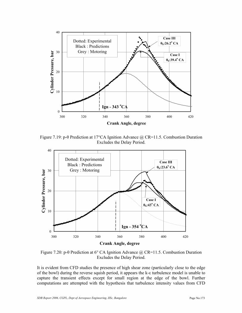
SDB Report 2006, CGPL, Dept of Aerospace Engineering, IISc, Bangalore Page No.173
0
10
20
30
40
300 320 340 360 380 400 420
Crank Angle, degree
Cyl
inde
r Pr
essu
re, b
ar
Dotted: ExperimentalBlack : Predictions
Grey : Motoring
Ign - 343 oCA
Case Iθb:39.4o CA
Case IIIθb:26.2o CA
Figure 7.19: p-θ Prediction at 17°CA Ignition Advance @ CR=11.5. Combustion Duration Excludes the Delay Period.
0
10
20
30
40
300 320 340 360 380 400 420
Crank Angle, degree
Cyl
inde
r Pr
essu
re, b
ar
Dotted: ExperimentalBlack : Predictions
Grey : Motoring
Ign - 354 oCA
Case Iθb:43o CA
Case IIIθb:23.6o CA
Figure 7.20: p-θ Prediction at 6° CA Ignition Advance @ CR=11.5. Combustion Duration
Excludes the Delay Period.
It is evident from CFD studies the presence of high shear zone (particularly close to the edge of the bowl) during the reverse squish period, it appears the k-ε turbulence model is unable to capture the transient effects except for small region at the edge of the bowl. Further computations are attempted with the hypothesis that turbulence intensity values from CFD

SDB Report 2006, CGPL, Dept of Aerospace Engineering, IISc, Bangalore Page No.174
studies are under-predicted during reverse squish period (post TC). The turbulence intensity considered for the pre-TC period is based on CFD results, for the post-TC period experimental trends of Catania et al [1996] shown in Figure 7.6 is adopted. The results corresponding to ignition setting of 17 and 12° CA at CR=17.0 are shown as Case II in Figures 7.14 and 7.16. The computed values show marginal improvement, but still the under-prediction appears to be large. Similarly the variation is found to be marginal in other four cases.
Upon further exploring the 0-D results (Case I) it became evident that in all the six test cases, major part of the combustion occurred during the reverse squish period wherein fluid dynamics within the combustion chamber is dominant. This point seems to indicate that the flow field during reverse squish period is enhancing the burn rate. This could well be so since there is steep increase in the cylinder pressure after a certain time, with a sharp pointed peak unlike a rounded peak at advanced ignition setting (Simple case). This called for a careful examination of the flow field generated from the CFD studies. The flow during the reverse squish period (366° CA) is shown in Figure 7.21, wherein mean and peak velocities are in the range of 8-12 m/s and 20 m/s respectively. The variation of squish velocity (from CFD) as a function of CA at the edge of the bowl is shown in Figure 7.22. This part has been discussed in Section 6.6 of Chapter VI. Under reacting conditions (with combustion) these velocities would be much higher, by an order of 2.0 –2.5 consistent with the ratio of Tburned to Tunburned).
20 m/s
C
C
D D
B
B
0
4
8
12
16
20
0 20 40 60 80 100Distance, mm
Spee
d,m
/s
B-BC-C
D-D
Speed Along The Dotted line
Figure 7.21: Vector Plot in the Diametric Plane at a Distance of 0.2 mm Below Cylinder Head at 366° CA. Dotted Circle Represents the Edge of the Bowl.

SDB Report 2006, CGPL, Dept of Aerospace Engineering, IISc, Bangalore Page No.175
-40
-30
-20
-10
0
10
20
30
40
300 325 350 375 400 425
Crank Angle, degree
Vel
ocity
, m/s
CFD @ 11.5CFD @ 17.0COR @ 12.0 COR @ 17.0COR @ 11.5
Reverse squish
Squish TC
Figure 7.22: Comparison of Squish Velocities from CFD and using an Empirical Correlation –COR [Heywood, 1988] at for the SPE Geometry (CR=17.0 and 11.5) and the MPE
Geometry (CR=12.0). Taking the fluid dynamics during reverse squish into account, a hypothesis is formed for flame propagation beyond the bowl region: the flame penetrates the flat section at the top with enhanced (depending upon the squish velocities around that time period) velocities, and then propagates into the unburned mixture at the same velocities in an annular cylindrical manner from the cylinder head downwards. This Reverse Squish Flame (RSF) hypothesis is pictorially depicted in Figure 7.23. With the RSF hypothesis computations are re-attempted, where in a flat annular flame is assumed to travel outwards subsequent to spherical flame engulfing the bowl. The flat annular flame is assumed to travel at a rate dictated by the local outgoing fluid velocities as shown in Figure 7.21.
Figure 7.23: Reverse Squish Flame (RSF) Hypothesis. (a) Flat Annular Flame Propagating Outward along the Cylinder Head (b) Axial View Showing Flat Flame Propagation Due to Outward Flow of Fluid. The Dotted Circle Shows the Trace of Spherical Flame on the Cylinder Head. Under reacting conditions, these velocities assume higher value in commensurate with the ratio Tburned/Tunburnted. All features of EELB flame propagation are taken valid except that flame shape is considered ‘Flat’. With these assumptions the predictions are better, shown as

SDB Report 2006, CGPL, Dept of Aerospace Engineering, IISc, Bangalore Page No.176
Case III for all test cases in Figures 7.14 to 7.20. The principal results are given in Table –7.8. It is evident that combustion duration is lower with RSF hypothesis compared to entirely spherical flame assumption. Table –7.8: Principal Results of ‘Complex - I’ Cases. Mass Burned Fraction (MBF) corresponds to 372° CA.
Case
Experiment Prediction Peak Pressure, bar
Occurrence, °CA
Peak Pressure, bar
Occurrence, °CA
Duration, °CA
MBF, %
CR=17.0, 17° CA I 67.4 369 52.0 370.8 37.2 84 III 67.4 369 59.0 372.8 30.0 100 CR=17.0, 12° CA I 75.6 371 47.1 372.4 37.4 72 III 75.6 371 57.0 374.4 26.4 92 CR=17.0, 6° CA I 54.5 379 39.2 375.0 35.4 42 III 54.5 379 43.7 380.8 26.8 56 CR=13.5, 14° CA I 45.0 376 33.2 373.2 52.6 62 III 45.0 376 37.5 379.2 33.4 80 CR=11.5, 17° CA I 37.5 372 30.5 373.0 48.4 66 III 37.5 372 35.8 378.4 35.2 88 CR=11.5, 6° CA I 25.0 383 24.0 377.6 52.0 39 III 25.0 383 25.5 383.6 23.6 52
The mass burned fraction (MBF) – including the entrained mass at the time of peak reverse squish effect (Case I – with spherical flame assumption) is given in Table – 7.8, which shows large variation in MBF for a given ignition setting at different CR’s. This clearly indicates that there is substantial amount of unburned fuel in the combustion chamber and all that is required is a mechanism to trigger the rapid energy release apart from normal flame propagation. One such theory proposed in this thesis is the RSF hypothesis; the predicted pressures with RSF hypothesis are better than entirely spherical flame assumption for all the six cases. The unburned fuel corresponding to 372° CA is relatively lower with RSF compared to spherical flame assumption according to Table 7.8. However, the peak pressures are lower, with point of occurrence at a later point compared to experiments. The predictions still do not simulate the steep rise in pressure; this therefore points towards fluid dynamics being too complex during reverse squish period and appears to wield a major influence in altering the burn rate. Here the author would like to reemphasize that this sudden act of rapid energy release is not an abnormal combustion, namely knock or surface ignition. This is argued not to be so because if it were to be so then it should have been evident at advanced ignition setting, wherein conditions are more favorable. Moreover, this sharp rise in pressure is not desirable because of its contribution to higher power output. Therefore, in the current context it is difficult to perceive the exact mechanism by which there is a sudden increase in burn rate, nevertheless the data point towards that. In addition to what has been proposed in the RSF hypothesis it is quite possible that the hot burned products flowing out of the bowl during reverse squish period are mixing with the unburned mixture in the flat region, which is followed by nearly instantaneous burning due to the thin tongue igniting. The change in the

SDB Report 2006, CGPL, Dept of Aerospace Engineering, IISc, Bangalore Page No.177
velocity distribution pattern in the flat part of the piston geometry as evident from Figure 7.24 (a) could result in large velocity gradient under reacting conditions. Such a situation could lead to formation of vortices, wherein the burned gas emerging out of the bowl (during peak of reverse squish period) could mix with the unburned mixture above the flat part of the piston geometry. The hypothesis is schematically depicted in Figure 7.24(b). This mechanism appears to be strongly dependent on the local fluid dynamics caused due to engine geometry and the piston movement. The factors that appear to dictate pressure rise in the later part of combustion are, the time of the spherical flame engulfing the bowl (whether coinciding with the reverse squish effect becoming dominant) - the magnitude of reverse squish velocity, amount of unburned mixture in the flat region of the combustion chamber and relative magnitude of energy release rate to cylinder volume changes. This argument appears to be consistent with the experimental p-θ data, wherein at an ignition timing of 17° CA (CR = 17.0), there is a sharp rise in the cylinder pressure, occurring over 2-3° CA, where as at 6° CA this is observed to occur over 7-8° CA. Further analyzing, at a less retarded ignition setting (17° CA), the amount of unburned mixture is lower; therefore mixing would be rapid, thus resulting in instantaneous burning.
360
CA
o
362
CA
o
370
CA
o
1.5 m/s- 25 m/s
- 5 m/s- 10 m/s
360.
3 C
Ao
(a)
Flat FlameBurned Gas gushing
out of bowl
Hot ProductsUnburned Mixture
(b)
Figure 7.24 (a) Velocity distribution close to the edge of the bowl (u component) - above Flat Region of the Piston at the end of squish period and in the Reverse Squish period (b) Hypothesis Depicting Burned Gas Outflow from the Bowl Into the Cylindrical Region During Reverse Squish Period. The Mixing of the Burned Gas with the Unburned Gas in the Presence of a Flat Flame Could Result in Rapid Burn Rate.
However, at retarded ignition setting (6° CA) the fraction of unburned mixture is relatively larger, thus requiring more time for mixing and as a consequence the heat release rate is gradual. Moreover, the thermodynamic conditions at less retarded ignition setting are favourable for steep rise in cylinder pressure. These observations are not that evident at low CR probably due to lower reverse squish velocities. A comparison of energy balance on similar lines to the earlier case is shown in Table 7.9. The predicted IPG improves with the RSF hypothesis at all ignition settings and CRs. The predicted heat loss through exhaust and coolant/wall compares reasonably with the experimental data and any marginal variation in these values is again attributed to the selection of the heat transfer coefficient. However, 17° CA corresponding to CR=11.5 is an exceptional case wherein the experimental heat loss is higher due large fraction of unburned CO (40%) constituting the exhaust energy.

SDB Report 2006, CGPL, Dept of Aerospace Engineering, IISc, Bangalore Page No.178
Table – 7.9: Comparison of Energy Balance (kW) of ‘Complex –I’ Cases
Mode IE IPG FL BPN FA FA Exhaust Coolant/Wall
CR=17.0, 17° CA
Ex-org 63.5 23.4 - 18.4 - - 19.0 26.1
Ex-red 63.5 23.4 1.1 18.4 1.4 2.5 16.9 22.2
0-D - I 63.5 21.7 1.3 NC NC NC 21.6 18.9
0-D -III 63.5 21.9 1.3 NC NC NC 21.3 19.0
CR=17.0, 12° CA
Ex-org 63.6 25.2 - 19.8 - - 17.0 26.8
Ex-red 63.6 25.2 1.1 19.8 1.4 2.9 15.9 22.5
0-D -I 63.6 22.0 1.3 NC NC NC 21.6 18.7
0-D -III 63.6 22.7 1.3 NC NC NC 20.9 18.7
CR=17.0, 6° CA
Ex-org 65.0 25.3 - 20.0 - - 18.5 26.5
Ex-red 65.0 25.3 1.2 20.0 1.4 2.8 17.3 22.3
0-D -I 65.0 21.1 1.3 NC NC NC 24.6 18.0
0-D -III 65.0 22.4 1.3 NC NC NC 23.2 18.0
CR=13.5, 14° CA
Ex-org 63.0 22.5 - 18.6 - - 24.5 19.9
Ex-red 63.0 22.5 1.1 18.6 1.4 1.4 23.4 17.1
0-D- I 63.0 19.5 1.3 NC NC NC 23.5 18.6
0-D -III 63.0 19.9 1.3 NC NC NC 22.8 19.0
CR=11.5, 17° CA
Ex-org 64.0 21.0 - 17.6 - - 27.6 18.8
Ex-red 64.0 21.0 1.1 17.6 1.4 0.9 26.5 16.5
0-D - I 64.0 19.9 1.3 NC NC NC 24.2 18.6
0-D -III 64.0 20.3 1.3 NC NC NC 23.4 19.0
CR=11.5, 6° CA
Ex-org 63.0 20.5 - 17.0 - - 25.2 20.8
Ex-red 63.0 20.5 1.2 17.0 1.4 1.0 24.0 18.4
0-D- I 63.0 18.9 1.3 NC NC NC 24.8 18.0
0-D- III 63.0 19.8 1.3 NC NC NC 23.3 18.6 Ex-org: original experimental results, Ex-red: redistributed results NC: Not Computed
Predictions of p-θ Curve – Complex –II Cases Two test cases at a fixed CR of 12.0 belonging to MPE are categorized under complex - II and their salient features are repeated in the Table 7.10 for ease of reference.

SDB Report 2006, CGPL, Dept of Aerospace Engineering, IISc, Bangalore Page No.179
Table –7.10: Principal Parameters of ‘Complex – II’ Cases
No.
CR
Composition, Vol, % Φ
RG %
Input* Energy/ cycle, kJ
Ign, °CA
Ign#. Delay, °CA
Category H2 CO CH4
12 12.0 19.5 19.0 0.6 0.91 8.5 3.25 19 8 Complex -II 13 12.0 18.5 19.0 0.5 0.91 8.5 3.25 12 5 Complex -II
Figure 7.25 Flame Kernel Displacement into the Bowl Due to the Effect of Squish Predictions are initially shown using simple spherical flame propagation model, followed by RSF hypothesis. An important aspect to be noticed in the combustion chamber is the location of ignition source i.e. spark plug. The spark plug in this particular geometry is located at an offset, which lies on a plane above the flat part of the piston. In the event of flame kernel formation after ignition, the flame kernel is bound to be exposed to higher velocities and there by get displaced deeper into the bowl as shown in Figure 7.25. Displacement of the flame as a consequence of squish phenomenon could be much more complex than what is accounted in the model. This could also be one of the reasons for ignition delay to be shorter compared to SPE test cases at corresponding ignition setting, despite fuel-air mixture being lean. Considering offset spark plug location, higher velocity is considered for the initial flame kernel movement, which is of the order of squish velocity (20 –25 m/s). At the end of the ignition delay period the flame kernel is assumed to be along the axis of the combustion chamber due to symmetry in the flow field. The methodology adopted for computation is the same as discussed earlier. The turbulence intensity considered in the model is higher by 25% than that of SPE, the length scale employed corresponds to that employed in CR=11.5. This part has been bought out in Section 7.7. For the flame movement, squish velocities obtained from CFD corresponding to CR=17.0 are used since bumping clearance in MPE is nearly same as that of SPE at the highest CR. All other geometric parameters with respect to the combustion chamber of MPE are adopted and the valve profile shown in Figure 7.4 is considered. All other parameters relating to Cd, and heat transfer coefficients adopted in the earlier predictions are taken valid for MPE. No additional resistance in the gas exhaust line caused due to the presence of the turbo-charger is considered, which essentially means flow through the turbo-charger is not modeled. However, for the purpose of calculations, the recorded charge pressure (experimental data) downstream of the turbo-charger is used as the intake manifold pressure. There the intake manifold pressure is assumed to be constant (1.25 bar) through the suction process of the calculations, since the variation in the manifold pressure could be marginal with a twelve-cylinder engine.

SDB Report 2006, CGPL, Dept of Aerospace Engineering, IISc, Bangalore Page No.180
Results
0
10
20
30
40
50
60
70
300 320 340 360 380 400 420
Crank Angle, degree
Cyl
inde
r Pr
essu
re, b
ar
Ign - 341o CA
Case Iθb:40.8o CA
Case IIIθb:23.6o CA
Dotted: ExperimentalBlack : Predictions
Grey : Motoring
Figure 7.26: p-θ Prediction at 19° CA Ignition Advance with MPE Geometry. Combustion Duration Excludes the Delay Period.
0
10
20
30
40
50
60
300 320 340 360 380 400 420
Crank Angle, degree
Cyl
inde
r Pr
essu
re, b
ar
Dotted: ExperimentalBlack : Predictions
Grey : Motoring
Ign - 349 oCA
Case Iθb:46.6o CA
Case IIIθb:25o CA
Figure 7.27: p-θ Prediction at 12° CA Ignition Advance with MPE Geometry. Combustion
Duration Excludes the Delay Period.
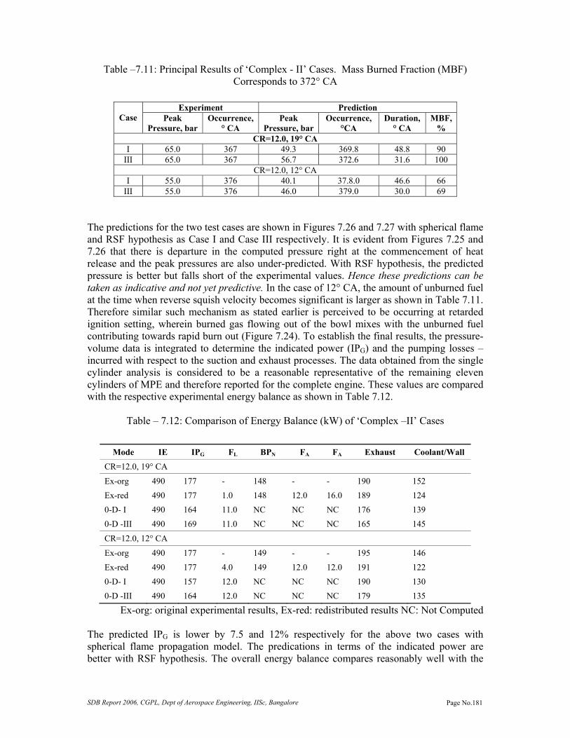
SDB Report 2006, CGPL, Dept of Aerospace Engineering, IISc, Bangalore Page No.181
Table –7.11: Principal Results of ‘Complex - II’ Cases. Mass Burned Fraction (MBF) Corresponds to 372° CA
Case Experiment Prediction
Peak Pressure, bar
Occurrence, ° CA
Peak Pressure, bar
Occurrence, °CA
Duration, ° CA
MBF, %
CR=12.0, 19° CA I 65.0 367 49.3 369.8 48.8 90
III 65.0 367 56.7 372.6 31.6 100 CR=12.0, 12° CA
I 55.0 376 40.1 37.8.0 46.6 66 III 55.0 376 46.0 379.0 30.0 69
The predictions for the two test cases are shown in Figures 7.26 and 7.27 with spherical flame and RSF hypothesis as Case I and Case III respectively. It is evident from Figures 7.25 and 7.26 that there is departure in the computed pressure right at the commencement of heat release and the peak pressures are also under-predicted. With RSF hypothesis, the predicted pressure is better but falls short of the experimental values. Hence these predictions can be taken as indicative and not yet predictive. In the case of 12° CA, the amount of unburned fuel at the time when reverse squish velocity becomes significant is larger as shown in Table 7.11. Therefore similar such mechanism as stated earlier is perceived to be occurring at retarded ignition setting, wherein burned gas flowing out of the bowl mixes with the unburned fuel contributing towards rapid burn out (Figure 7.24). To establish the final results, the pressure-volume data is integrated to determine the indicated power (IPG) and the pumping losses – incurred with respect to the suction and exhaust processes. The data obtained from the single cylinder analysis is considered to be a reasonable representative of the remaining eleven cylinders of MPE and therefore reported for the complete engine. These values are compared with the respective experimental energy balance as shown in Table 7.12.
Table – 7.12: Comparison of Energy Balance (kW) of ‘Complex –II’ Cases
Mode IE IPG FL BPN FA FA Exhaust Coolant/Wall
CR=12.0, 19° CA
Ex-org 490 177 - 148 - - 190 152 Ex-red 490 177 1.0 148 12.0 16.0 189 124 0-D- I 490 164 11.0 NC NC NC 176 139 0-D -III 490 169 11.0 NC NC NC 165 145
CR=12.0, 12° CA
Ex-org 490 177 - 149 - - 195 146 Ex-red 490 177 4.0 149 12.0 12.0 191 122 0-D- I 490 157 12.0 NC NC NC 190 130 0-D -III 490 164 12.0 NC NC NC 179 135
Ex-org: original experimental results, Ex-red: redistributed results NC: Not Computed The predicted IPG is lower by 7.5 and 12% respectively for the above two cases with spherical flame propagation model. The predications in terms of the indicated power are better with RSF hypothesis. The overall energy balance compares reasonably well with the

SDB Report 2006, CGPL, Dept of Aerospace Engineering, IISc, Bangalore Page No.182
experimental data, however the computed pumping losses are higher compared to experimental results. The uncertainty in the discharge coefficients of the valves of this engine is possibly the reason for this discrepancy. Further refinement is not attempted because the error in experimental measurement of pumping loss is fairly large, as it is obtained as the difference between two nearly equal quantities while integrating the p-v curve. Sensitivity Analysis Among the assumptions considered for 0-D predictions as stated in section 7.4, heat transfer coefficients for different processes were essentially obtained by matching one of the test cases against its corresponding result. The overall energy balance comparison is found to be reasonable in most cases. Similarly value of Cd for the gas exchange process was obtained by matching against motoring curve. This leaves apart the combustion wall temperature, which is considered at a fixed value of 450 K for all the processes. A sensitivity analysis considering 25° C variation in the wall temperature does not influence the results significantly (IP variation by < 0.5%). Further sensitivity analysis is considered in terms of varying the laminar burning velocity (+ 10%), turbulence intensity (+10%) and ignition delay (+3° CA). Test case belonging to CR=17.0 corresponding to an ignition timing of 22° CA is considered as reference and results are shown in in Figs. 7.28 to 7.30. The predicted pressures are marginally lower with the reduction in the laminar burning velocity and turbulence intensity. However, the rate of heat release seems to be different with different ignition delay periods. Any variation in the predicted pressure should ultimately impact the indicated output. From the results summarized in Table 7.13, it is clear that 10% variation in laminar burning velocity and turbulence intensity has very little influence on the IPG, similarly variation in the ignition delay period lowers the output by about 3%.
Table- 7.13: Sensitivity Analysis towards IPG (kW) Prediction at 22° CA
Exp IPG 0-D nominal SL, m/s u’, m/s θdelay, ° CA -10% +10% -10% +10% -2 +2
22.4 21.8 21.75 21.71 21.70 21.73 21.0 21.2
0
10
20
30
40
50
60
70
300 320 340 360 380 400 420
Crank Angle, degree
Cyl
inde
r Pr
essu
re, b
ar
Dotted: ExperimentalBlack : Predictions
Grey : Motoring
Ign - 338 oCA
LS (10% lower)LS (10% higher)
Figure 7.28: p-θ Prediction at 22° CA Ignition Advance with + 10% Variation in SL

SDB Report 2006, CGPL, Dept of Aerospace Engineering, IISc, Bangalore Page No.183
0
10
20
30
40
50
60
70
300 320 340 360 380 400 420
Crank Angle, degree
Cyl
inde
r Pr
essu
re, b
arDotted: Experimental
Black : PredictionsGrey : Motoring
Ign - 338 oCA
(10% lower)
(10% higher)tu
tu
Figure 7.29: p-θ Prediction at 22° CA Ignition Advance with + 10% Variation in u’
0
10
20
30
40
50
60
70
300 320 340 360 380 400 420
Crank Angle, degree
Cyl
inde
r Pr
essu
re, b
ar
Dotted: ExperimentalBlack : Predictions
Grey : Motoring
Ign - 338 oCA
(2o CA lower)delayθ
delayθ (2o CA higher)
Figure 7.30: p-θ Prediction at 22° CA with Different Ignition Delay Period

SDB Report 2006, CGPL, Dept of Aerospace Engineering, IISc, Bangalore Page No.184
Observations The findings of 0-D model are summarized in Table 7.14. In the four simple cases identified, the 0-D model is able to make reasonably good predictions by assuming the conventional spherical flame propagation model. The accuracy in IP prediction is around 3% for CR=17.0 and 11.5, and between 5 and 8% for the other two cases at CR=13.5. Among the six cases dealt under complex-I category, predictions appear to be better by assuming the RSF hypothesis. In fact the accuracy in the IP computation improves in all the six cases. Similar is the trend with Complex – II cases. Table 7.14: Summary of 0-D Predictions for Different Test Cases. Turbulence Intensity Results from CFD Analysis and ref - Experimental Results on an Engine with Similar Configuration [Catania et al, 1996]. The Flame Shape Accounted in the Prediction both Inside and Outside the Bowl is Also Given.
Case No.
Flame Shape - Region u’ 0-D# Error, %
Inside Bowl Outside Bowl Pre-TC Post-TC
Simple
1 Spherical CFD 1.5
2 Spherical CFD 3.0
6 Spherical CFD 5.0
7 Spherical CFD 8.0
9 Spherical CFD 3.2
Complex – I & II
3 Case I Case III
Spherical Spherical
Spherical Flat
CFD CFD
CFD ref
8.0 6.0
4
Case I Case III
Spherical Spherical
Spherical; Flat
CFD CFD
CFD ref
13.0 10.0
5 Case I Case III
Spherical Spherical
Spherical Flat
CFD CFD
CFD ref
16.0 11.4
8 Case I Case III
Spherical Spherical
Spherical Flat
CFD CFD
CFD ref
13.0 11.5
10 Case I Case III
Spherical; Normal
Spherical Flat
CFD CFD
CFD ref
5.2 3.3
11 Case I Case III
Spherical Spherical
Spherical Flat
CFD CFD
CFD ref
8.0 3.0
12 Case I Case III
Spherical Spherical
Spherical Flat
CFD CFD
CFD ref
7.5 4.5
13 Case I Case III
Spherical Spherical
Spherical Flat
CFD CFD
CFD ref
10.0 7.3
# Error is defined as the ratio of computed IPG to Experimental IPG
Summarizing the 0-D prediction qualitatively, the 0-D model is able to make reasonably accurate predictions at advanced ignition settings (above 17° BTC) using classical EELB heat

SDB Report 2006, CGPL, Dept of Aerospace Engineering, IISc, Bangalore Page No.185
release sub-model. However, at retarded ignition setting (< 17° BTC) the enhanced fluid dynamics due to reverse squish flow modifies the burn rate to such an extent that there is a steep rise in cylinder pressure. By making use of the insight obtained from the cold flow CFD studies a hypothesis namely, Reverse Squish Flame (RSF) has been formulated wherein the outgoing fluid is assumed to modify the flame shape from spherical to flat. With this hypothesis the predictions are better but still differ from the experimental values both qualitatively and quantitatively. An interesting point to be brought is the large fraction of unburned fuel at such a point beyond which there is rapid release of energy. The exact mechanism by which rapid energy release is occurring is not clear; however a few indicators towards such possibility have been brought out. Therefore fluid-flame interaction is sufficiently complex and predictions with simpler techniques like 0-D model are not possible. This calls for a full-fledged 3-D modeling with combustion for further understanding.
Summary 0-D predictions are presented for twelve test cases of two engine geometries at different CRs by categorizing them according to their intricacies. The overall energy balance has been compared against the experimental results. These show a good agreement for cases of lower compression ratio and advanced ignition timings. For other cases, additional hypothesis are invoked and ways of improving the predictions are explored.

SDB Report 2006, CGPL, Dept of Aerospace Engineering, IISc, Bangalore Page No.186
Chapter VIII Adaptation of Cummins Gas Engines for Use with Gasifiers for Power Generation In continuation of the efforts towards development of producer gas engines, a collaborative effort was launched in 2003 along with Cummins India Ltd, Pune for adapting their natural gas engines for producer gas operation. Two of the natural gas engines were successfully operated with producer gas and long duration trails successfully conducted in the laboratory. The details of the test summary are presented in this chapter. Introduction Cummins India Ltd, Pune are the largest manufacturers of diesel engines in India and also have large presence in the area of natural gas engines. Cummins manufacturers a range of gas engines in the capacity between 75 kWe to 500 kWe suiting natural gas fuel. They also supplied/converted a number of buses in New Delhi to operate on CNG fuel along with their sister concern Tata Cummins. They have a strong network of marketing and servicing agencies throughout the country. They have a large manufacturing facility at Pune with a separate department dedicated for research and development. Considering some of these positive strengths, CGPL expressed their willingness in collaborating with Cummins in the area of gas engines. Since Cummins were not fully convinced about gasification technology and the use of producer gas in their gas engines, it was decided that two different model gas engines are jointly tested at the laboratory prior to deploying in the field for commercial operations. The agencies involved in this testing programme are (i) CGPL, IISc – have been involved in development of biomass gasification technology over two decades (ii) Cummins India Ltd, pune – leaders in stationary power-generating set in India and overseas, and (iii) NETPRO – licensed manufacturer of IISc’s biomass gasifier and immediate beneficiary of this testing programme. Test Procedure The two different models of gas engines tested in the laboratory, one was a naturally aspirated engine and other a turbo-charged after-cooled engine. The specifications of these engines are presented in Table 8.1.

SDB Report 2006, CGPL, Dept of Aerospace Engineering, IISc, Bangalore Page No.187
Table 8.1: Gas Engine Specifications
Make and Model Cummins, G743G Cummins, GTA855G
Engine Type In-line, 6 cylinder, 4-stroke, Naturally Aspirated Gas Engine
In-line, 6 cylinder, 4-stroke, Turbocharged-aftercooled Gas Engine
Rated Output - 1500 Rev/Min @ sea level
101 kW with natural gas 160 kW with natural gas
Net Output* - @ Bangalore ~ 1000m above sea level
84 kW, with natural gas 84 kW, with natural gas
Bore x Stroke, mm 130 x 152 140 x 152
Total Displacement, L 12.1 14.0
Specific Power, kW/L
7.0 (with NG) 11.0 (with NG)
Compression Ratio (CR) 10 8.5
Combustion Chamber Flat cylinder head and a Shallow Bowl-in piston type
Squish Area 35%
Spark Plug Type & Location - Gas Mode
Central
Conversion/mo-dification, if any Producer Gas Carburetor adapted
Ignition system - gas Battery based distributor type with ignition advance/retard facility
Governor Woodward Hydraulic
Spark plug & location - gas
Champion make, Central
Firing order 1-5-3-6-2-4
Alternator Efficiency 92%
Conversion/mo-dification, if any Producer Gas Carburetor adapted * Net Output – after deducting power drawn by engine accessory drives
The objective of the test program was to evaluate the performance of the Cummins gas engines coupled to the open top gasifier developed by Indian Institute of Science and in particular to evaluate the gas quality ingested into the engine. The naturally aspirated engine was tested extensively and also involved a 24-hour continuous trail, whereas the turbo-charged model was tested at about 70% of its rated capacity. The in-house designed producer gas carburetor developed at IISc was fitted on the gas engine (natural gas carburetor removed). The arrangement of the gas carburetor along with the pressure regulator is similar to the one shown in Figure 8.1. The Schematic of the testing arrangement is shown in Figure 8.1. The clean producer gas was made available at the exit of the fabric filter for the operation of gas engine. The gas was made available at a pressure of 300- 500 mm wg above the ambient pressure. Further, fuel-line arrangement to the gas engine includes a pressure regulator and a gas carburetor. The combination of pressure regulator and gas carburetor was located between the gasifier and the engine intake system as shown in Figure 8.1. The zero pressure regulator ensures a gas

SDB Report 2006, CGPL, Dept of Aerospace Engineering, IISc, Bangalore Page No.188
pressure (downstream of the pressure regulator) identical to that of air pressure and this is achieved by connecting the air pressure line (down stream of air filter) to the upper chamber of the regulator. This arrangement ensures the regulator to maintain the gas pressure close to that of air pressure (~ a few mm below atmospheric pressure) and thereby the set air/fuel ratio irrespective of the total mixture flow rate.
Figure 8.1: Schematic showing gasifier coupled to the gas engine
The parameters monitored during the gas engine operation included the following:
• Fuel gas composition – H2, CO, CH4, CO2 and O2 – to estimate the lower calorific value of the fuel gas
• All relevant pressure, temperature on the gasification system • Biomass consumption • Quality of the producer gas being supplied to the engine – by drawing a sample gas at
the gasifier exit and bubbling through a solvent and further passing through a cellulose filter paper.
• Also, another qualitative check was conducted with respect to the quality of the producer gas. This involved checking the internal passages of the gas engine like the throttle, manifold and some parts of cylinder head were observed for any dust/tar deposition prior to and after the tests.
• Input and output pressures at the pressure regulator-gas carburetor • Exhaust gas composition – NO, CO, SO2, O2 and temperature

SDB Report 2006, CGPL, Dept of Aerospace Engineering, IISc, Bangalore Page No.189
• Engine parameters – coolant temperature, oil pressure, ignition timing • Load measurements – electric power in kWe, frequency, energy meter reading. Power
factor = 1.0 – resistive heating load. • The internal passages of the gas engine like the throttle, manifold and some parts of
cylinder head were observed for any dust/tar deposition prior to and after the tests. During these tests, all the parameters related to engine and the gasifier system was manually recorded at 30 min intervals. A mixture of wood chips and coconut shells was used as the fuel. The G743G model engine was run for about 23 hours and about 18 hours of continuous operation, with an average load of 49 ± 2 kWe and frequency in the range of 48.5 – 49 Hz. The GTA855G was tested for about 10 hours duration at about 80 kWe. Test Details The gasifier system was initially stabilized in flare mode for about 2 hours and subsequently the producer gas was supplied to the gas engine. The Cummins executives reviewed the engine condition in accordance to the test procedure and the gas engine operations were commenced. The engine was started with producer gas – air mixture and operated at no-load for few minutes and subsequently electrical load was applied to the engine-alternator in steps till about 50 kWe @ 48-48.5 Hz. The ignition timing was set at 22° BTC and verified using ignition timing light. During the initial one hour of engine operation, the load was varied in order to examine the governor response and control. Load throw-off trails using 6, 12, 18 and 24 kW block load were also conducted and the engine responded well maintaining the frequency between 48.5 and 51.5 Hz. The engine operation was found to be steady and smooth. After six hours of operation, the engine was stopped and the intake manifold was dismantled and examined. The butterfly valve and the intake manifold were found to be clean except for extremely fine carbon particles in very small quantities. Further, the components were refitted without cleaning (except for a small sample collected in the manifold using a tissue paper) and engine operations were resumed. The engine was operated at constant set load of 47 kWe @ 48.5-49 Hz for another 18 hours. The testing was stopped after successful completion of 24 hrs of testing. Results and observations The engine operation was found to be smooth and steady. During this operation the exhaust temperature was lower than 495 °C and water temperature well below 77° C. After the 24-hour run, the butterfly valve and intake manifold were reexamined for any physical deposition. The observation was similar to that at the end of 6 hrs of run. Further, these fine deposits were washed using ethanol and washings collected for gravimetric analysis. Also, 250 ml of engine lubricant was collected for analysis to be conducted by Cummins. The spark plug was also examined at the end of the run and its condition was found to be satisfactory according to Cummins. The resistance of the spark plug after undergoing about 80 hours of testing is as follows : 8.5, 10.2, 9.6, 8.6, 10.9, 10.4 kohms. The spark plugs were examined and found normal. Lubricating oil was sampled for further analysis. Photographs of various components were taken before and after the test are shown in Plate 8.1. All the recording of the test trials are plotted in Figures 8.2-8.5.

SDB Report 2006, CGPL, Dept of Aerospace Engineering, IISc, Bangalore Page No.190
30
35
40
45
50
55
12.00
P.M
12.25
P.M
12.55
P.M
1.25 P
.M
1.55 P
.M
2.25 P
.M
3.00 P
.M
3.45 P
.M
4.30 P
.M
5.15 P
.M
6.50 P
.M
7.30 P
.M
8.15 P
.M
9.00 P
.M
10.30
P.M
12.00
A.M
1.30 A
.M
3.00 A
.M
4:30 A
M
6:00 A
M
7:30 A
M
9.00A
.M
10:30
AM
12:00
PM
Time in hours
Load
, Fre
quen
cy
Frequency, HZ
Load, kWe
Figure 8.2: Load and Frequency with Time
0
200
400
600
800
1000
1200
1400
12:00
12:35 1:2
02:3
03:3
54:3
55:4
07:1
08:0
59:0
110
:3211
:55 1:00
2:10
3:25
4:40
6:15
7:30
8:3510
:0011
:0012
:25
Time in hours
Cum
ulat
ive
Bio
mas
s co
nsum
ptio
n, k
g
Figure 8.3: Biomass consumption with Time

SDB Report 2006, CGPL, Dept of Aerospace Engineering, IISc, Bangalore Page No.191
0
5
10
15
20
25
30
12:00
pm
12:45
pm
1:30p
m
2:15p
m
3.00p
m
3:45p
m
4:30p
m
5:15p
m
6:00p
m
6:30p
m
7:15p
m
8:00p
m
8:45p
m
10:00
pm
11:30
pm
1:00a
m
2:30a
m
4.00a
m
5.30a
m
7.00a
m
8.30a
m
10.00
am
11:30
AM
Time in hours
Gas
com
posi
tion,
%CO
H2
CO2
O2
Figure 8.4: Producer Gas Composition with Time
0
0.2
0.4
0.6
0.8
1
0 4 8 12 16 20 24Time, Hours
NO
, g/M
J
0
0.4
0.8
1.2
1.6
2
CO
, g/M
J
CO
NO
Figure 8.5: Variation of emission at 90% load during 24 hours of continuous operation.

SDB Report 2006, CGPL, Dept of Aerospace Engineering, IISc, Bangalore Page No.192
Plate 8.1
Butterfly Valve, Intake Manifold and Cylinder head
Initial After 6 Hours After 24 Hours
After 24 hours Test ……
Spark Plug Hour meter
Plate 8.2

SDB Report 2006, CGPL, Dept of Aerospace Engineering, IISc, Bangalore Page No.193
After 24 hours Test ……
Washing from Intake Manifold and Gas Bubbler and Cellulose Filter Butterfly Valve
Cummins officials interacting with IISc Team during the 24-hr testing
Cummins officials examining the gas engine after the 24-hr testing

SDB Report 2006, CGPL, Dept of Aerospace Engineering, IISc, Bangalore Page No.194
Chapter IX Development of Environmentally Clean Applications with Biomass Gasifiers for Power Generation This chapter reports the application and status of the producer gas engine based biomass power plant that are operational in the field as on January 2005. The performance of 1 x 125 kWe system and 5 x 125 kWe systems is reported and important functional parameters namely the specific biomass consumption and the maximum engine rating are brought out. Also the engine exhaust emission measured over long duration is reported. Introduction As on January 2005, producer gas engines were operational at five sites. The installed capacity of these five plants is 2.275 MWe. The capacities of the gas engines are 15, 55, 125 and 250 kWe. Of these engines, 55 to 250 kWe belong to Cummins make. The one at 15 kWe is a diesel–convert-gas engine and is functional at Dewan Farm Estate, Bethmangala, Kolar district, Karnataka. The details of the eleven sites are given in the Table 9.1.
Table 9.1 Rating of Producer gas engine plants
Power level, kWe
Application Month of commissioning
Hours Run Address
1 x 16 Captive December 2000 1800 Dewan Estate, Bethmangala, Kolar dist., Karnataka
1 x 55 Captive December 2004 2000 Desi Power Orchcha Pvt. Ltd. Taragram, Orchcha, Tigila, Orchcha District Tikamgarh, M.P. 472246
1 x 130 ESCO August 2003 7000 Bhagavathi Bio Power C/o United bleaching Ltd., Nelturai Road, Metupalyam, Coimbatore District
1 x 130 Captive July 2004 350 PSG College of Technology P.B. No. 1611, Peelamedu Coimbatore – 641004
5 x 250 Grid linked December 2004 5400 cumulative
Arashi Hi-tech Biopower Pvt. Ltd., No. 76, Patel Road, Ramnagar, Coimbatore-641009
3 x 250 Captive March 2005 1000 Cumulative
Hatsuns Pvt. Ltd, Kancheepuram.
2 x 80 + 2 x 160
Captive April 2005 1000 Cumulative
Hindustan Pencils Ltd, Jammu
1 x 130 Water pumping
January 2005 Initial trials completed
Water Works division, Kushalnagar, Karnataka
2 x 250 Water pumping
June 2005 Initial trials completed
Water Works division, Bethmangala, Karnataka
1 x 130 Captive April 2005 150 RV College of Engg Bangalore
1 x 50 Captive Feb 2005 200 Jawaharlal Nehru College of Engg., Shimoga
The performance of three plants of 15, 120 and 5 x 250 kWe capacity are discussed in detail in the following paragraphs

SDB Report 2006, CGPL, Dept of Aerospace Engineering, IISc, Bangalore Page No.195
Gas engine of 16 kWe at Dewan Estate, Bethmangala, Kolar district: A 50 kg/hr biomass gasifier has been installed by M/ NETPRO, Bangalore (Licensee of IISc gasifiers), at Dewan Estate (80 km from Bangalore), Bethamangala, Kolar district of Karnataka state for power generation application. The gasifier system operates two engine-alternator sets, one a standard 20 kWe rated diesel engine to operate on dual-fuel mode and a 16 kWe gas engine to operate on 100% producer gas. The electricity generated from these two units is used for energizing 5 x 7 hp irrigational pump sets scattered in a radius of about of 1.5 km. The estate is spread in an area of about 100 acres with coconut and horticulture being their main crop. The agro- wastes from the farm like coconut shells, fronds, casurina are being used as the feedstock in the gasifier. The gasifier system is essentially an IISc down draft reactor coupled with appropriate cooling and cleaning system. The exit of the gasifier system branches to two of the individual engine-alternator sets. One of these engines is a 100% producer gas engine, essentially converted from a standard diesel engine of 20 kWe capacity (Kirloskar, RB-33 make). The diesel engine has been modified at the existing compression ratio of 17:1 to work as a spark ignition engine by replacing the fuel injectors with spark plugs and adopting a distributor based ignition system. This engine delivers a peak of about 16 kWe on 100% producer gas. The engine is provided with a gas governing system to take care of the load variations. Plate 9.1 shows the installation.
Plate 9.1: The 100% producer gas engine at Dewan Estate Performance The gasifier system was commissioned in the month of May 2000 and subsequently the gas engine was commissioned in August 2000. Plantation residue in form of coconut shells, fronds and waste wood is used as the feedstock in the gasifier. The system is operated in an intermittent mode whenever there is requirement of irrigation water. On an average the gas engine is operated for about 3-4 hours per day at about 12- 14 kWe. As on January 2005, the system has completed nearly 2500 hours of operation. Cumulative number of units generated

SDB Report 2006, CGPL, Dept of Aerospace Engineering, IISc, Bangalore Page No.196
is in excess of 50,000. Some aspects of the engine performance have been reflected in Figure 9.1, which shows the specific biomass consumption against several days of operation.
0.8
1
1.2
1.4
1.6
1.8
2
0 20 40 60 80 100Cumulative days
kg/k
Wh
Figure 9.1: Specific biomass consumption of gas alone mode (dispersion due to load variations) for farm land electricity generation for deep borewell water pumping
Currently the system is in operation and is being intermittently used on a daily basis (3-4 hour/day). Increase in no. of hours of operation to 6 hours /day normally happens once a year occurs during sugar cane harvest season, wherein the electricity is utilized for operating the crusher for in-house jaggery production. Also, the user has used electricity for illuminating the farm house for about 3-4 hours in the evenings. Gas engine of 120 KWe at Bagavathi Biopower Ltd, Metupalyam, Coimbatore This gas engine is deployed in an Energy Service Company (ESCO), which sells green electricity to a textile industry. The company named Bagavathi Biopower Limited is located at Metupalyam in South India, near the city of Coimbatore. The plant has been supplied and installed by Energreen Power Limited, Chennai (Licensee of IISc gasifiers). The power plant is configured with a 150 kg/hr gasifier coupled with a GTA855G (Cummins) gas engine. The plant is also provided with an effluent treatment plant and an engine-waste-heat based biomass drier. The plant commissioned in September 2003 has successfully completed over 6000 hours (until January 2005) of operation. It took about three months to stabilize the plant operations, subsequently; the plant has been operating 24 x 6 days a week at an average load of 110 – 125 kWe, with a peak load of 134 kWe.

SDB Report 2006, CGPL, Dept of Aerospace Engineering, IISc, Bangalore Page No.197
Plate 9.2 Overview of the gasifier plant at Metupalyam
Plate 9.3 Gas engine with indigenous gas
carburetor Performance Julifora Prosopsis is the biomass that is being currently used at a specific consumption of 1.1 kg/kWh. In addition to electricity, value addition product namely partly activated carbon is also generated to an extent of 6-8%. The carbon has a typical Iodine number of 500 – 550 and has a market value of 0.5 USD/kg. The gas engine is being jointly monitored by IISc and Cummins, India and periodically inspected once every 1000 hours of operation. These inspections have shown the engine components (throttle valve, compressor of turbo-charger, after-cooler, intake manifold, intake valves and spark plug) to be clean and intact.
The particulate matter collected in these components amount to 25-30 microgram/Nm3. Measurement of the engine exhaust have shown the CO and NOx levels to be much lower than most of the emission norms of various countries. The current operating cost (fuel + manpower + maintenance) per unit electricity generated is about 4 US Cents with return on investment at about 15 %. Plate 9.2 & Plate 9.3 shows the overview of the gasifier plant and the gas engine respectively. Similarly Figure. 9.2 highlights the no. of hours operated by the system month-wise during Aug ’03 to Feb ’05. The plant took about four months for stabilization, wherein the no. of hours of operation was lower. The stabilization period was slightly longer because of issues related to load management. Subsequent to that the no. of hours of operation was around 400 hours except for few months during the onset of monsoon, wherein procuring dry biomass became a major bottleneck. At this juncture the flue gas based biomass dryer was installed. Once the dryer was installed, dry biomass was available on a continuous basis. The subsequent rise and fall in the no. of hours were more related to non-availability of plant load and has little to do with the availability of the plant for operations. The plant has completed nearly 7200 hours of operation as on May 2005. The gas engine has been inspected by Cummins R&D team on three occasions and has found the operations to be reasonably clean and satisfactory. They have suggested lube oil change once in 500-600 hour of operation.
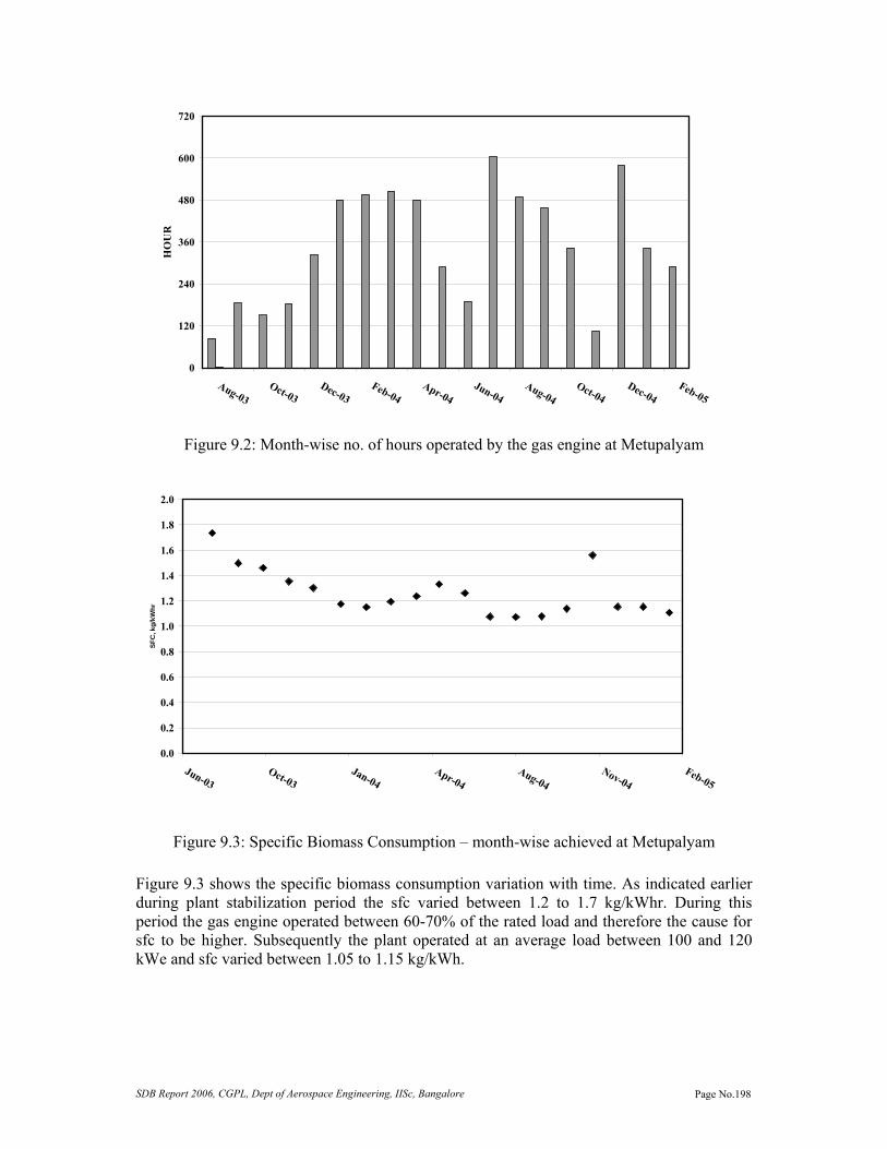
SDB Report 2006, CGPL, Dept of Aerospace Engineering, IISc, Bangalore Page No.198
0
120
240
360
480
600
720
Aug-03Oct-03
Dec-03Feb-04
Apr-04Jun-04
Aug-04Oct-04
Dec-04Feb-05
HO
UR
Figure 9.2: Month-wise no. of hours operated by the gas engine at Metupalyam
0.0
0.2
0.4
0.6
0.8
1.0
1.2
1.4
1.6
1.8
2.0
Jun-03Oct-03
Jan-04Apr-04
Aug-04Nov-04
Feb-05
SFC
, kg/
kWhr
Figure 9.3: Specific Biomass Consumption – month-wise achieved at Metupalyam Figure 9.3 shows the specific biomass consumption variation with time. As indicated earlier during plant stabilization period the sfc varied between 1.2 to 1.7 kg/kWhr. During this period the gas engine operated between 60-70% of the rated load and therefore the cause for sfc to be higher. Subsequently the plant operated at an average load between 100 and 120 kWe and sfc varied between 1.05 to 1.15 kg/kWh.
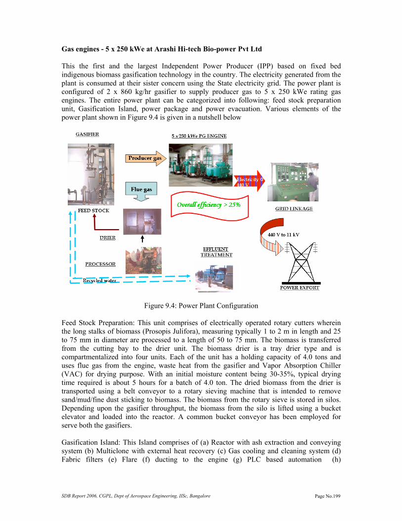
SDB Report 2006, CGPL, Dept of Aerospace Engineering, IISc, Bangalore Page No.199
Gas engines - 5 x 250 kWe at Arashi Hi-tech Bio-power Pvt Ltd This the first and the largest Independent Power Producer (IPP) based on fixed bed indigenous biomass gasification technology in the country. The electricity generated from the plant is consumed at their sister concern using the State electricity grid. The power plant is configured of 2 x 860 kg/hr gasifier to supply producer gas to 5 x 250 kWe rating gas engines. The entire power plant can be categorized into following: feed stock preparation unit, Gasification Island, power package and power evacuation. Various elements of the power plant shown in Figure 9.4 is given in a nutshell below
Figure 9.4: Power Plant Configuration Feed Stock Preparation: This unit comprises of electrically operated rotary cutters wherein the long stalks of biomass (Prosopis Julifora), measuring typically 1 to 2 m in length and 25 to 75 mm in diameter are processed to a length of 50 to 75 mm. The biomass is transferred from the cutting bay to the drier unit. The biomass drier is a tray drier type and is compartmentalized into four units. Each of the unit has a holding capacity of 4.0 tons and uses flue gas from the engine, waste heat from the gasifier and Vapor Absorption Chiller (VAC) for drying purpose. With an initial moisture content being 30-35%, typical drying time required is about 5 hours for a batch of 4.0 ton. The dried biomass from the drier is transported using a belt conveyor to a rotary sieving machine that is intended to remove sand/mud/fine dust sticking to biomass. The biomass from the rotary sieve is stored in silos. Depending upon the gasifier throughput, the biomass from the silo is lifted using a bucket elevator and loaded into the reactor. A common bucket conveyor has been employed for serve both the gasifiers. Gasification Island: This Island comprises of (a) Reactor with ash extraction and conveying system (b) Multiclone with external heat recovery (c) Gas cooling and cleaning system (d) Fabric filters (e) Flare (f) ducting to the engine (g) PLC based automation (h)

SDB Report 2006, CGPL, Dept of Aerospace Engineering, IISc, Bangalore Page No.200
Instrumentation (i) effluent treatment plant. Items (a) – (h) are in 2 nos., where as effluent treatment plant is a common facility for both the gasifiers. Power Package & Power Evacuation: The power package comprises of 5 x 250 kWe Cummins gas engine (GTA 1710G) adapted to operate on producer gas fuel. The engines is provided with electronic governor and coupled to 380 kVA alternator to generate electricity at 415 V. There is synchronizing panel provided with necessary protections to synchronize each of the generator set with the State grid at 415 V. Further the power is stepped up to 11 kV using a 2 MVA transformer and evacuated to the State grid. Performance: As indicated earlier, the power plant houses two gasifiers coupled to 5 x 250 kWe gas engine sets. The First gasifier (Gasifier A) was commissioned in August 2002. This system was initially coupled with a 1 MWe diesel generator set. Subsequently in June 2004, the diesel engine was replaced with gas engines. Also, an additional gasifier, Gasifier B was commissioned in October 2004. The two gasifiers were operated in tandem with five gas engines and have recorded a maximum output of 1.1 MWe. This power plant performance was closed monitored for about 30 hour duration, wherein a number of parameters related to gasifier and gas engine was continuously monitored. Some of the performance charts are shown in Figure. 9.5 to 9.7. The producer gas contained 20-22% of CO and H2, 1.5 – 2% CH4. As evident from Figure 9.5 the variation in the gas composition is minimal with Lower Calorific Value (LCV) of the gas being 4.8 MJ/kg
0
4
8
12
16
20
24
0 5 10 15 20 25Time, hrs
Gas
Com
posi
tion,
%
0
1
2
3
4
5
6
LC
V, M
J/kg
COH2CH4LCV
T0=18 hrs of 12/1/05
Figure 9.5 Producer gas composition with time. Plot shows gas composition after correcting
for the small fraction of oxygen contained in the gas.

SDB Report 2006, CGPL, Dept of Aerospace Engineering, IISc, Bangalore Page No.201
0
200
400
600
800
1000
1200
0 2 4 6 8 10 12 14 16Time, hrs
Gro
ss u
nits
gen
erat
ed
T0= 18.00 hrs on 12.01.05
Figure 9.6: Gross units generated with time
0.0
0.2
0.4
0.6
0.8
1.0
1.2
1.4
1.6
0 2 4 6 8 10 12 14 16
Time, hrs
Sp. b
iom
ass
cons
ump,
kg/
kWh
Figure 9.7: Specific biomass Consumption with time

SDB Report 2006, CGPL, Dept of Aerospace Engineering, IISc, Bangalore Page No.202
Table 9.2: Exhaust emissions
Time Genset Temp CO O2 NO, ppm NO2, ppm NOx
SO2
% g/MJ ppm g/MJ ppm mg/MJ
18.30 1 400 0.324 1.62 6.2 331 4 331 0.17 55 27.5
19.30 2 450 0.134 0.56 1.9 282 1 283 0.12 41 17.0
20.30 3 450 0.171 0.77 3.0 118 0 118 0.05 33 14.9
21.30 4 425 0.116 0.5 2.4 268 2 270 0.12 22 9.5
22.30 5 425 0.109 0.5 3.5 105 0 105 0.05 20 9.3 Figure 9.6 and 9.7 shows the gross electricity generated by the power plant and the specific biomass consumption during that period. The internal consumption of the plant was between 20 and 22%, which is inclusive of auxiliary load like plant & office illumination etc. The specific biomass consumption (based on gross electricity generated) was between 1.0 and 1.2 kg/kWhr. The exhaust emission recorded on the five gas engine sets is shown in Table 9.2, the NO and CO levels are much below the norms specified by CPCB. The SO2 in the exhaust is accountable only from the engine lube oil as producer gas doesn’t contain sulfur or its oxides. Table 9.3 summarizes the no. of hours operated by each engine and the gross electricity generated between June ’04 and July ’05. There is no shown for engines 4 & 5 up to November 2004 because the related gasifier i.e gasifier B was commissioned at the end of December 2005. As of July 2005, the five engines have recorded a cumulative run of over 15,000 hours.
Table 9.3 Month wise no. of hours of operations and units generated at Arashi Hi-tech Bio-power Pvt Ltd
Month Engine 1 Engine 2 Engine 3 Engine 4 Engine 5 Total Gen.
Hrs Gen Hrs. Gen Hrs. Gen. Hrs Gen Hrs Gen
June.04 - - 156.5 22253 164.4 22351 - - - - 44604
July.04 - - 212.6 31999 205 31160 - - - - 63159
Aug. 04 196.4 34630 415.9 83619 - - - - - - 118249
Sep.04 521.7 93730 441.2 67650 3.8 - - - - - 161380
Oct.04 431.3 84800 221.3 26700 39.2 5670 -- - - - 117170
Nov.04 587.6 109200 12.7 1600 540.7 84719 - - - - 195519
Dec.04 395.1 60300 43 5400 335.2 44770 8 382 36 5127 115979
Jan.04 521 88562 358.9 62283 381.8 59211 309.2 55377 50.8 10066 275499
Feb.04 174 28810 139.7 20126 271.9 40844 76.9 14479 306.6 55908 160167
Mar.04 411.1 60839 422.7 66710 380.3 62869 408 62905 461.9 67327 320650
Apr.04 200.4 32524 526.5 89045 285.8 50286 328.2 52693 442.1 72326 296874
May.05 14.00 2733 329.6 60608 166.2 32312 49.3 7948 441.6 78745 182346
June.05 128.4 19530 441.9 68119 128.3 23881 147.6 23600 398.5 69524 204654
July.05 214.2 38086 226.4 36089 559.5 96967 429.8 69107 382.5 65037 305286
Total hrs. 3795.2 3848.9 3462.1 1757.0 2520
Total gen 653744 642201 555040 286491 424060 2561536

SDB Report 2006, CGPL, Dept of Aerospace Engineering, IISc, Bangalore Page No.203
Observations By March ’05 the total installed capacity of producer gas engine power plants is abut 3.6 MWe. Of these about six plants are operated in a continuous mode for commercial operations, two plants installed at engineering college operates intermittently either as a back-up power unit or for academic purpose. The remaining three plants are yet into come into regular stream of operation. One other plant that need to be noted are the four gas engine sets installed at Jammu, which operate on a gasifier fuelled with sawdust briquette. As of July 2005, there is cumulative experience of over 25,000 hours available from eight plants, serving in various modes of operation. All this success have been achieved well within two years of collaborative effort with Cummins and therefore much could be expected in times to come.

SDB Report 2006, CGPL, Dept of Aerospace Engineering, IISc, Bangalore Page No.204
Chapter X Overview In this final chapter, the principal contributions of the present work have been highlighted. The areas in which further work in the next phase of activity could be pursued are brought out. Contribution of the Present Work The first principal contribution of the present work is the revelation of non-knock performance of producer gas in high compression ratio (CR) spark-ignited engine. Earlier to this work, the general perception was that producer gas would knock when operated in high CR spark-ignited engine. This perception has been proved to be incorrect by making systematic investigations on a 20 kW rating (SPE) spark ignition engine converted from a production diesel engine at varying compression ratios of 17, 14.5, 13.5 and 11.5. The engine operation was found to be smooth at the highest CR of 17.0 without any undesirable effects of knock as discerned from the pressure-crank angle (p-θ) curve, which showed smooth rise in pressure without any pressure oscillations. However, there was de-rating of the engine power, which is about 16.7% at a CR of 17.0 and increased to 26% at a CR of 11.5. Maximum net power (excluding power consumed by fan and accessories) is recorded at a fuel-air equivalence ratio of 1.08 + 0.2, with gas to useful shaft power conversion efficiency being 30.7 and 27.5% respectively for the highest and lowest CR. The reduction in power output with producer gas is attributed to reduction in the net calorific value of the fuel gas and air mixture, and to the net reduction in number of molecules as the mixture goes to product gases. In terms of emissions, the NOx level are well below the emission norms in India and abroad, the CO level is found to be higher when operated at slightly fuel rich conditions where maximum power is delivered. However, the CO levels will be within norms when the engine is operated at stoichiometry or slightly leaner condition. The second level of testing attempted on the 250 kW (MPE) gas engine revealed smooth operations at the designed CR=12.0. The de-rating on this engine was found to be about 21% compared with diluted natural gas operation on similar engine. The emission in terms of NOx and CO is well below than all existing emission norms. The lower CO content with this engine is attributed to better air-to-fuel ratio control. Another important outcome from this experimental work is that the optimum ignition timing for producer gas operation is retarded compared to natural gas operation at comparable CR. This is attributed to higher laminar burning velocity of producer gas compared to natural gas. The high laminar burning velocity contributed to faster combustion as a result; there is low cycle-to-cycle variation in the indicated mean effective pressure (IMEP) at all CRs and ignition timings. In the modelling part, a zero-dimensional (0-D) model is constructed to simulate the processes of a spark-ignition engine operation. The heat release part, which is key to the modelling, is based on the well-postulated Eddy Break-up and Laminar Burn-up model meant for turbulent pre-mixed wrinkled flames. The two key input parameter sets for the heat release sub-model are derived from further computations. The laminar burning velocity data, at pressures and temperatures encountered in an engine combustion chamber is obtained from computations based on a one dimensional flame code. The turbulence parameters, namely, turbulent intensity and integral length scale are obtained from three-dimensional CFD computations for engine combustion chamber geometry, involving bowl-in piston

SDB Report 2006, CGPL, Dept of Aerospace Engineering, IISc, Bangalore Page No.205
arrangement at CR of 17.0 and 11.5. These turbulence parameters are further assumed to undergo variations under reacting conditions by using simple rapid distortion process as stated in the literature. The in-cylinder pressure predictions are made by incorporating data on laminar burning velocity, turbulence parameters and flame displacement from the above-mentioned computations. One experimental firing case is used as a test case in tuning the 0-D model in terms of constants required for computation of heat loss. Subsequently, keeping these parameters fixed 0-D predications are made for twelve test cases involving combustion chambers of SPE and MPE at varying CRs and ignition settings. These are further categorized under three sub-groups, namely Simple, Complex I and Complex II depending upon the intricacy involved in the predictions. Under the Simple sub-group four test cases of SPE are dealt, wherein the predictions match very well with the experimental p-θ curve. These computations are attempted assuming simple spherical flame propagation model. Whereas, under Complex-I and II sub-group eight cases are dealt, wherein the cylinder pressures are under-predicted with simple spherical flame propagation model. It is observed that in most of these cases, a major part of the combustion occurred during the reverse squish period, wherein the enhanced fluid movement could be modifying the burn rate to substantially high values. The exact mechanism by which it is occurring is not clear, nevertheless an indicator towards that has been formulated, which is termed as ‘Reverse Squish Flame’. Under this hypothesis the enhanced fluid movement is assumed to modify the burn rate. Predictions with this hypothesis are better but falls short of experimental results. An interesting point to be brought is the large fraction of unburned fuel at such a point beyond which there is rapid release of energy. The exact mechanism by which rapid energy release is occurring is not clear, but full computation of reacting flow field is expected to reveal this. At this stage one might like to ask about the usefulness of the 0-D model in a general way. The answer to this is as follows. Most of the engines built for gaseous fuel like the natural gas are of CR 12.0 and below. And moreover, most of the gas engines are designed for lean-burn operation and therefore adopt complex shaped geometries (eg. bowl-in piston), supported with a centrally located spark plug to enhance the burn-rate. The optimum ignition advance for these fuels is between 24 – 28° BTC. These conditions permit a flow-field that would have marginal role of reverse squish in modifying the burn-rate. In all such cases the methodology developed here would provide ‘good’ predictions (within a few percent). Also, joint collaborative work with Cummins India for the adaptation of natural gas engines for producer gas is reported. As a consequence of this joint work, a number of systems are operating in the field on semi-commercial and commercial modes. Scope for Future Work A fair amount of work on producer gas engines have been accomplished in the first phase of the project particularly on modeling of the in-cylinder processes, optimum ignition advance at various compression ratios, and development of carburetor for producer gas operation. As a result of these investigations, it has been possible to introduce producer gas engines of capacities ranging from 20 kW to 250 kW in the field. There would some derating of the engine capacity with producer gas operation compared to natural gas operation, for which these engines were originally designed. However the extent of derating can be reduced by properly selecting the compression ratio and through proper choice of turbocharger. The work in the first phase has shown that significantly higher compression ratio can be used for producer gas operation without the adverse effects of knocking compared to many other fuels. However, turbo charging has not been looked into during the first phase of the project.

SDB Report 2006, CGPL, Dept of Aerospace Engineering, IISc, Bangalore Page No.206
The turbocharger works best when the engine is operating close to its peak power; but its effectiveness drops steeply as the engine works under part load. Hence when an engine designed for natural gas is run with producer gas, its power output is reduced both because of the reduced heating value of the gas-air mixture and due to the reduced effectiveness of the turbocharger. The operating point of the turbocharger shifts to possibly a non-optimal point because of the shift in the conditions of the gas (temperature and pressure) entering the turbine. To examine these issues, maps of the characteristics of the compressor and the turbine, along with a suitable engine model for predicting the outlet conditions of the gas from the engine cylinder, in addition to the power output. The characteristics of the commercially available turbochargers are in general not available and hence they have o be generated by conducting tests on them. Hence, it is proposed to set up a turbocharger test facility, which has the capability of generating the compressor and turbine characteristics. A few turbochargers of varying capacities would be tested in this facility and along with the engine model, the peak power output and efficiencies at full and part loads would be predicted and results validated for the available engines. This model can then be utilized for adapting available gas engines for producer gas operation.

SDB Report 2006, CGPL, Dept of Aerospace Engineering, IISc, Bangalore Page No.207
Chapter XI Non-Edible Seed-Oils for Power Generation with Engines in Single or Dual Fuel Mode This chapter reports the laboratory scale experiments done for power generation with engines using non-edible oils in single or dual fuel mode. Introduction
Non-Edible oils are fast gaining prominence as an alternate to diesel as the calorific value and Cetane number of the non-edible oils in their pure form are comparable to diesel oil. The changeover from diesel to Non edible oil is considered relatively simple; however, the impediments are their high viscosity. In the light of this, the present study is conducted in order to investigate engine performance and the exhaust emissions using various non-edible oils as fuel, in pure form as well as their blends, in direct injection (DI) diesel engine. The primary aim is to arrive at a basic strategy that can be adopted for reducing emission levels using these fuels.
The basic strategies reported in the literature are: 1) Adaptation of the engine to the fuel by modifying engine to suit fuel properties (particularly its viscosity and Cetane number) by making engine adiabatic, changing lubricant/ coolant, lubrication system, increase injection pressure etc 2) Adaptation of the fuel to the engine by modifying physico-chemical properties by blending or trans-esterification. Utilizing these strategies in an appropriate way can lead to the most practical and economical methodology that can ease the required swift changeover from diesel to bio-derived oils. In addition certain experiments are tried to dual fuel the engines with producer gas and find out the non-edible oil replacements achievable.
Literature Survey
Gopalkrishna and Rao (1985), Bhasker et al. (1992), Subramaniyam and Jayaraj (1994) have conducted engine tests using vegetable oils in a semi-adiabatic engine and have found reduced particulate emissions and increase in brake thermal efficiencies. Elsbett Engine [1] developed by a private engine researcher based on the first strategy is capable of utilizing raw vegetable oils. However, this engine is about two and a half times more expensive. Although the trans-esterification of triglycerides is an established process for reducing fuel viscosity and improving Cetane number (Ma and Hanna, 1999, Srivastava and Prasad, 2000), it is not clear if it is essential for application in the rural areas. Keeping these facts in view, a more practical and economical strategy involving both the strategies need to be explored. Blending of the fuel with alcohol will not only reduce viscosity but will oxygenate fuel
Experiments In the present investigation, ethanol, a bio-derivative, is used as a blender with various vegetable oils with primary aim of reducing viscosity and emissions. The volume of ethanol was restricted to 5 % in order to prevent expected deterioration of engine performance at peak load because of reduction of fuel heating value and cetane number, caused by addition of ethanol (heating value 22 ~ 25 MJ/kg).

SDB Report 2006, CGPL, Dept of Aerospace Engineering, IISc, Bangalore Page No.208
Most pure vegetable oils have kinematic viscosity in the range of 30 to 40 cSt at 30 C, volumetric heating value in the range of 39 to 40 MJ/kg and cetane number in the range of 32 to 40 (Srivastava and Prasad, 2000). The blend with ethanol (5 %) has kinemtic viscosity in the range of 21 – 22 cSt. The comparison of properties for various oils is shown in Table 11.1. Table 11.1: Non-edible oil properties
Fuel Type
Calorific Value, (MJ/kg)
Specific Gravity At 25 C
Viscosity at 27 C, N.s/m2
Cetane No
Diesel 42.3 0.815 0.13 47a
Repeseed Oil 37.62 0.914 39.5 37.6a Pongamia Oil 35.8 0.94 1.22 - Jatropha oil 36.0 0.92 1.1 - Esterified Jatropha 36.5 0.90 0.52 -
It was physically observed that sprays of both, vegetable oil as well as their blends with ethanol, obtained at standard injection pressure of 180 bar was very coarse and contained large droplets in the spray core. When the spray was ignited, a lot of single particle combustion was physically observed, indicating larger droplets in the spray. This, however, had a reducing trend when injection pressure was increased up to 350 bar. A 3.5 kWe direct injection, naturally aspirated water cooled diesel engine (cylinder diameter of 80 mm and stroke of 110 mm) with a compression ratio of 17 running at a nominal speed of 1500 rpm with the injection timing set at 13° was used in the present study: The nominal injector pressure was 180 atms.
The experimental set up is shown in the Figure 11.1.
Figure 11.1: Schematic of experimental set-up for the test
Cooling Water Tank
Exhaust
DI Engine Alternator
Loading Panel
Gas Sample line Gas Analyser
Fuel Container
Filters

SDB Report 2006, CGPL, Dept of Aerospace Engineering, IISc, Bangalore Page No.209
Except for the change in injection pressure and timing, there were no changes made in the engine. Injection pressure was varied from 180 – 340 bars. A standard fuel nozzle tester was used to characterize the spray.
A Single Phase AC alternator was coupled to the engine main shaft and a resistance coils/light bulbs were used to load the engine. The fuel flow rate/ consumption was directly measured by taking fuel level drop in a metering jar and corresponding time for the set injector pressure. The injection timing was based on the point of ejection of fuel from the three holes of the injector and not at the fuel pump exit plane, as is considered in common practice. This is due to the observed injection delay that sets in when injection pressure is increased in the range of present study. The observed difference is about 6° – 8° at 180 bars and this difference increases at higher pressure.
Fuel injection was advanced up to 35° by increasing the effective length of the fuel pump plunger by 1.8 mm without affecting it fuel-metering performance. Injection delay with respect to the maximum advance was obtained by introducing thin slip disk between the pump body and engine body.
A K-type thermocouple was used to measure exhaust gas temperature at the location close to the point from where sample gas was drawn for analysis. Quintox flue gas analyzer was used to measure CO, CO2, O2, NOx, SOx and HC (hydrocarbon) concentrations in engine exhaust. The gas was cooled, filtered and dried prior to analyses.
The vegetable oil and their blends were injected at room temperature. No emulsion stabilizers were added to fuel blends since the emulsion was prepared just before its use and was completely consumed. The fuel was filtered by allowing it to pass through the tandem of standard diesel filters prior to pumping.
Results and Discussions
The first sets of experiments were conducted in order to study effect of increasing injection pressure on engine exhaust emissions at varying loads. The injection delay was set to manufacturer’s standard 13° BTDC. The vegetable oils used were Pongemia (Karanjia), Mahauva, Neem, Hippe and Rapeseed obtained from market. Experiments with cold and hot (70 0C) caster oil were also successfully conducted. Oil from Cashew was also used however; this oil had very adverse effect on the fuel injection system causing immediate damage to the injector needle and fuel delivery valve. The experimental results of diesel, neem oil and neem oil blend consumption at various loads is shown in Table 11.2.
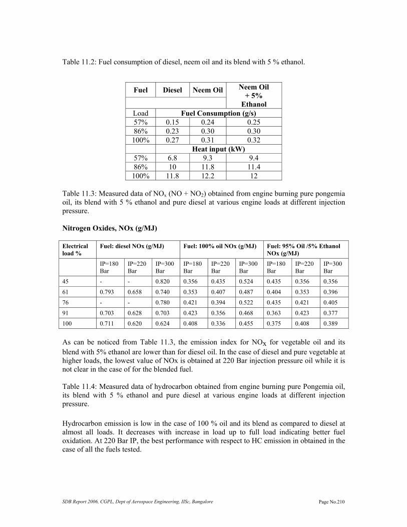
SDB Report 2006, CGPL, Dept of Aerospace Engineering, IISc, Bangalore Page No.210
Table 11.2: Fuel consumption of diesel, neem oil and its blend with 5 % ethanol.
Fuel Diesel Neem Oil Neem Oil + 5%
Ethanol Load Fuel Consumption (g/s)57% 0.15 0.24 0.25 86% 0.23 0.30 0.30 100% 0.27 0.31 0.32
Heat input (kW) 57% 6.8 9.3 9.4 86% 10 11.8 11.4 100% 11.8 12.2 12
Table 11.3: Measured data of NOx (NO + NO2) obtained from engine burning pure pongemia oil, its blend with 5 % ethanol and pure diesel at various engine loads at different injection pressure. Nitrogen Oxides, NOx (g/MJ)
As can be noticed from Table 11.3, the emission index for NOx for vegetable oil and its blend with 5% ethanol are lower than for diesel oil. In the case of diesel and pure vegetable at higher loads, the lowest value of NOx is obtained at 220 Bar injection pressure oil while it is not clear in the case of for the blended fuel. Table 11.4: Measured data of hydrocarbon obtained from engine burning pure Pongemia oil, its blend with 5 % ethanol and pure diesel at various engine loads at different injection pressure.
Hydrocarbon emission is low in the case of 100 % oil and its blend as compared to diesel at almost all loads. It decreases with increase in load up to full load indicating better fuel oxidation. At 220 Bar IP, the best performance with respect to HC emission in obtained in the case of all the fuels tested.
Electrical load %
Fuel: diesel NOx (g/MJ) Fuel: 100% oil NOx (g/MJ) Fuel: 95% Oil /5% Ethanol NOx (g/MJ)
IP=180 Bar
IP=220 Bar
IP=300 Bar
IP=180 Bar
IP=220 Bar
IP=300 Bar
IP=180 Bar
IP=220 Bar
IP=300 Bar
45 - - 0.820 0.356 0.435 0.524 0.435 0.356 0.356
61 0.793 0.658 0.740 0.353 0.407 0.487 0.404 0.353 0.396
76 - - 0.780 0.421 0.394 0.522 0.435 0.421 0.405
91 0.703 0.628 0.703 0.423 0.356 0.468 0.363 0.423 0.377
100 0.711 0.620 0.624 0.408 0.336 0.455 0.375 0.408 0.389

SDB Report 2006, CGPL, Dept of Aerospace Engineering, IISc, Bangalore Page No.211
Table 11.5: Measured data of CO obtained from engine burning pure Pongamia oil, its blend with 5 % ethanol and pure diesel at various engine loads at different injection pressure.
CO emission is lowest for diesel oil as compared to vegetable oil and its blend. This can be related to fuel viscosity effect. There seems to be a favorable effect of increase in injection pressure in the case of diesel and oil emulsion. However, there is no obvious effect in the case of pure oil. As compared to pure oil, oil emulsion seems to be combusting better
Table 11.6: Measured data of SOx obtained from engine burning pure Pongemia oil, its blend with 5 % ethanol and pure diesel at various engine loads at different injection pressure.
SOx has negligibly small value in case of diesel oil while in the case of 100 % oil and its blend it is detected at full or near full load. There is no obvious effect of increase in injection pressure on SOx emission except for in the case of oil with 5 % ethanol where the value becomes negligibly small.
The results for other non-edible oils are displayed in the Figures 11.2 to 11.4.
Electrical load %
Fuel: diesel HxCx (g/MJ)
Fuel: 100% oil HxCx (g/MJ)
Fuel: 95% Oil /5% Ethanol HxCx (g/MJ)
IP=180 Bar
IP=220 Bar
IP=300 Bar
IP=180 Bar
IP=220 Bar
IP=300 Bar
IP=180 Bar
IP=220 Bar
IP=300 Bar
45 - - 1.384 0.562 0.537 0.501 0.835 0.825 0.825
61 0.814 0.664 1.189 0.327 0.409 0.418 0.661 0.468 0.727
76 - - 1.110 0.272 0.321 0.332 0.450 0.354 0.584
91 0.612 0.442 1.085 0.260 0.278 0.289 0.389 0.322 0.460
100 0.383 0.401 1.146 0.360 0.272 0.269 0.361 0.273 0.415
Electrical load %
Fuel: diesel CO%
Fuel: 100% oil CO%
Fuel: 95% Oil /5% Ethanol CO%
IP=180 Bar
IP=220 Bar
IP=300 Bar
IP=180 Bar
IP=220 Bar
IP=300 Bar
IP=180 Bar
IP=220 Bar
IP=300 Bar
45 - - 0.052 0.088 0.084 0.082 0.095 0.100 0.090
61 0.0.41 0.057 0.041 0.088 0.081 0.078 0.089 0.082 0.086
76 - - 0.033 0.098 0.088 0.100 0.110 0.074 0.061
91 0.05 0.045 0.035 0.111 0.119 0.122 0.155 0.100 0.066
100 0.07 0.062 0.051 0.200 0.222 0.222 0.197 0.115 0.090

SDB Report 2006, CGPL, Dept of Aerospace Engineering, IISc, Bangalore Page No.212
0
0.1
0.2
0.3
0.4
0.5
0.6
0.7
Ponga
miaNee
mHipe
Mahuv
a
Rapes
eed
Diesel
NO
x (g
/MJ)
Injection Pressure = 220 BarInjection timing = 13o BTDC
Figure 11.2: NOx emissions with various oils
0
0.05
0.1
0.15
0.2
0.25
0.3
0.35
0.4
0.45
Ponga
miaNee
mHipe
Mahuv
a
Rapes
eed
Diesel
Hx C
x (g/
MJ)
Full LoadInjection Pressure = 220 BarInjection timing = 13o BTDC
Figure 11.3: HxCx emissions with various oils

SDB Report 2006, CGPL, Dept of Aerospace Engineering, IISc, Bangalore Page No.213
0.000
0.050
0.100
0.150
0.200
0.250
0.300
0.350
Ponga
miaNee
mHipe
Mahuv
a
Rapes
eed
Diesel
CO
(%)
Full LoadInjection Pressure = 220 BarInjection timing = 13o BTDC
Figure 11.4: CO emissions with various oils
Dual fuel operation with producer gas and no-edible oil Limited numbers of experiments were conducted in duel fuel mode at different operating conditions. The Figure 11.5 shows the percentage of diesel replacement in duel fuel mode using diesel and pongemia at various fuel injection advance. The extent of diesel saved seems to improve with advancement in fuel injection timing from 35-39° BTDC. However the extend of diesel saved at 35° timing is low against recorded in the earlier work. The reason for low replacement is due to poor producer gas composition. This becomes evident from the tests at 32°CA, where the diesel saved is relatively higher as compared to 35° CA data on account of superior gas composition.
3035404550556065707580
0 2 4 6 8 10 12 14 16 18 20
PG + PR.GAS at 31.3Deg BTDCDS + PR.GAS at 35 degBTDCDS + PR.GAS at 31.3 DegBTDCPG + PR.GAS AT 31.3deg BTDCPG + PR.GAS at 39 degBTDCDS + PR.GAS at 39 degBTDC
Figure 11.5: Liquid fuel replacement at various loads at different conditions

SDB Report 2006, CGPL, Dept of Aerospace Engineering, IISc, Bangalore Page No.214
The amount of diesel saved seems to improve with the advancing of injection timing on account of a larger time being made available for combustion and there by leading to better conversion efficiency. The extent of diesel saved at 39° CA is not very high and it might be possible to achieve higher replacement in longer duration operation where the gas quality substantially improves with the time. The reason for replacement being higher at 32°CA as against standard timing at 31° CA could be attributed only to better producer gas composition. Conclusion Studies on non-edible fuel oil have been conducted and its property with respect to atomization and emissions has been conducted. The dual fuel with pongemia oil has been performed and compared with diesel at various injection timing. It has been found that liquid fuel replacements at various loads and injection timing of pongemia and diesel are comparable.

SDB Report 2006, CGPL, Dept of Aerospace Engineering, IISc, Bangalore Page No.215
Nomenclature
Abbreviations
ABC After Bottom Centre ATC After Top Centre BBC Before Bottom Centre BC Bottom Centre BP Brake Power bsfc Brake Specific Fuel Consumption BTC Before Top Centre CA Crank Angle CFD Computational Fluid Dynamics CFR Cooperative Fuel Research CGPL Combustion Gasification and Propulsion
Laboratory CI Compression Ignition COV Coefficient of Variation CPCB Central Pollution Control BoardCR Compression Ratio DNS Direct Numerical Simulation EELB Eddy Entrainment and Laminar Burn-Up FET Filling and Emptying Technique FIP Fuel Injection Pump FSR Flame Speed RatioGHG Green House Gas HUCR Highest Useful Compression Ratio IGN Ignition Timing IISc Indian Institute of Science IMEP Indicated Mean Effective Pressure INJ Injection TimingIP Indicated Power LCV Lower Calorific Value LES Large Eddy Simulation MBT Minimum Advance for Brake Torque MPE Medium Power level Engine NG Natural Gas P & T Particulate and Tar PG Producer Gas PIV Particle Image Velocimetry p-v Pressure-Volume p-θ Pressure-Crank Angle RG Recycled Gas RSF Reverse Squish Flame RSV Reverse Squish Velocity S Separation Zone SI Spark Ignition SPE Small Power level Engine T Torroidal structure TC Top Centre TKE Turbulence Kinetic Energy 0-D Zero –Dimension

SDB Report 2006, CGPL, Dept of Aerospace Engineering, IISc, Bangalore Page No.216
Symbols
A Area Af Frequency Factor a,b Heat transfer Coefficients B Body Force C Concentration Cd Discharge Coefficient c Specific Heat of Gas D Bore Da Damkohler Number dQ Heat loss E Internal Energy e Specific Internal Energy FA Power Consumed by Accessories FL Pumping Loss FR Frictional Loss g Term Accounting for Expansion/Contraction of
Grid H Total Enthalpyh Specific EnthalpyJ Mass Flux k, λ Thermal Conductivity LT Total Losses lI Integral Length Scale lk Kolmogorov Length ScalelM Taylor Micro Scalel T Characteristic Length m Mass
bm.
Mass Burn Rate
p Pressure R Characteristic Gas Constant Re Reynolds Number S Burning Velocity T Temperature t Time U Velocity x Co-ordinate α Crank Angle μ Parametric/Entrained Mass ε Turbulence Dissipation Rate � Fuel-Air Equivalence Ratio k Turbulence Kinetic Energy ψ Recycled Gas r Radius u’ Turbulence Intensity uT Characteristic Speed V Volume Y Mass Fraction of Species δL Laminar Flame Thickness η Efficiency ρ Density τb Characteristic Time ώ’’’ Volumetric Production/Consumption Rate σ Stress Tensor μ Viscosity

SDB Report 2006, CGPL, Dept of Aerospace Engineering, IISc, Bangalore Page No.217
Subscripts
G Gross N Net p Pressure,
Products v Volume f Flame b Burned Gas L Laminar m Mixture, Mean u Unburned Gas w Wall i Species mech Mechanical T Turbulent o Reference

SDB Report 2006, CGPL, Dept of Aerospace Engineering, IISc, Bangalore Page No.218
References
1. Abdel-Gayed R. G. and Bradley B. (1976): “Dependence of Turbulent Burning Velocity on Burning Velocity to RMS Turbulent Velocity”, Proceedings Sixteenth International Symposium on Combustion, The Combustion Institute, pp-1725-1735.
2. Abraham J., Williams F.A. and Bracco F.V. (1985): “A Discussion of Turbulent Flame Structure in Premixed Charges”, SAE 850345, Vol. 94, pp. 128-143.
3. Annand W. J. D. (1963): “Heat Transfer in the Cylinders of Reciprocating Internal Combustion Engines”, Proceedings Institution of Mechanical Engineers, Vol. 177, pp. 973-990.
4. Anon (1986): “Wood gas as engine fuel”, A Report of the Mechanical Wood Products Branch of FAO Forestry Paper No. 72, Food and Agriculture Organization of United Nations, Rome.
5. Arcoumanis C., Bicen A.F. and Whitelaw J.H. (1983): “Squish and Swirl-Squish Interaction in Motored Model Engines”, Journal of Fluid Engineering, ASME, Vol. 105, pp. 105-112.
6. Arcoumanis C. and Whitelaw J.H. (1987): “Fluid Mechanics of IC Engines: A Review”, Proceedings Institution of Mechanical Engineers, Vol. 201.
7. Ballal D. R. and Lefebvre A.H. (1974): “Turbulence Effects on Enclosed Flames”, Acta Astronautica, Vol. 1, pp. 471-483.
8. Baruah P.C. (1986): “Combustion and Cycle Calculations in Spark Ignition Engines“, in the Thermodynamics and Gas Dynamics of Internal Combustion Engines, Vol. 2, pp. 823-865.
9. Bauer W, Heywood J.B., Avanessian O. and Chu D. (1996), “Flow Characteristics in Intake Port of Spark Ignition Engine Investigated by CFD and Transient Gas Temperature Measurements”, SAE 961997, Vol. 105, pp. 2110-2117.
10. Bicen A.F., Vafidis C., and Whitelaw J.H. (1985): “Steady and Unsteady Air Flow Through the Intake Valve of Reciprocating Engine”, Journal of Fluid Engineering, ASME, Vol. 107, pp. 413-426.
11. Blizard N. C. and Keck J.C. (1974): “Experimental and Theoretical Investigation of Turbulent Burning Model for Internal Combustion Engines”, SAE 740191, Vol. 83, pp. 846-864.
12. Blumberg P.N., Lavoie G.A. and Tabaczynski R.J. (1979): “ Phenomenological Models for Reciprocating Internal Combustion Engines”, Proceedings Energy Combustion Science, Vol. 5, pp. 123-167.
13. Borgnakke C. (1984): “Flame Propagation and Heat Transfer in SI Engines”, J Hillard and GS Springer (Eds), Fuel Economy in Road Vehicles Powered by SI Engines, Chapter 5, Plenum press, pp. 183-224.
14. Brokaw R.S. (1961): “Alignment Charts for Transport Properties, Viscosity and Diffusion Coefficients for Non-polar Gases Mixtures at Low Density”, Technical Report TRR-81, NASA.
15. Caris D.F. and Nelson E.E. (1959): “A New Look at High Compression Engines”, SAE Transactions, Vol. 67, pp. 112-124.

SDB Report 2006, CGPL, Dept of Aerospace Engineering, IISc, Bangalore Page No.219
16. Catania A. E. and Spessa E. (1996): “Speed Dependence of Turbulence Properties in a High-Squish Automotive Engine Combustion System”, SAE 960268, Vol. 105, pp. 313-334.
17. Chakravarthy P., Mishra D.P., Paul P.J. and Mukunda H.S. (1993): “The Theoretical Calculations of the Limits of Flame Propagation for Producer Gas Mixture”, Proceedings Fourth National Meet on Biomass Gasification and Combustion, Vol. 4, pp. 28-37.
18. Corcione F.E. and Valentino G. (1994): “Analysis of in-Cylinder Flow Processes by LDA”, Combustion and Flame, Vol. 99, pp. 387-394.
19. Das A. and Watson H.C. (1997): “Development of a Natural Gas Spark Ignition Engine for Optimum Performance”, Proceedings Institution of Mechanical Engineers, Part D, Vol. 211, pp. 361-378.
20. Duclos J.M., Bruneaux G., Baritaud T.A. (1996): “3D modelling of combustion and pollutants in a 4-valve SI engine; Effect of fuel and residuals distribution and spark location”, SAE 961964, Vol. 105, pp. 2048-2062.
21. Einewell P. and Johansson B. (1997): “Combustion Chambers For Supercharged Natural Gas Engines”, SAE 970221, Vol. 106, pp. 408-433.
22. Ekchian A. and Hoult D.P. (1979): “Flow Visualization Study of Intake Process of an Internal Combustion Engine”, SAE 790095, Vol. 88, pp. 383-399.
23. Fanslar T.D. (1985): “Laser Velocimetry Measurements of Swirl and Squish Flows in an Engine with a Cylindrical Piston Bowl”, SAE 850124, Vol. 94, pp. 1.747-1.763.
24. Fleischer F., Grosse W. and Zapf H. (1981): “Fuels From Biomass and Their Rational Utilisation in Internal Combustion Engines”, Proceedings International Conference - New Energy Conversion Technologies and Their Commercializations, Vol. 2, pp. 1334-1340.
25. Floch A, Franck J.V. and Ahmed A. (1995): “Comparison of the Effects of Intake Generated Swirl and Tumble on Turbulence Characteristic in a 4-Valve Engine”, SAE 952457, Vol. 104, pp. 2239-2255.
26. French C. C. J, Atkins K.A. (1973): “Thermal Loading of a Petrol Engine”, Proceedings Institution of Mechanical Engineers, Vol. 187, 49, pp 561-573.
27. Gatowski J.A., Heywood J. B. and Deleplace C. (1984): “Flame Photographs in a Spark-Ignition Engine”, Combustion and Flame, Vol. 56, pp. 71-81.
28. Giordano P. (1999): “Experience on Running a Wood Based Co-generation Power Plant with The IISc-Dasag Gasifier”, Biomass Users Network (BUN-India), Vol. 3.2, p. 2.
29. Gish R.E., McCullough J.D., Retzloff J.B. and Mueller H.T. (1958): “Determination of True Engine Friction”, SAE Transactions, Vol. 66, pp. 649-661.
30. Gordon and McBride (1975): “Method of Calculating Equilibrium Composition, Adiabatic Flame Temperature, Rocket Performance and Detonation”, NASA SP 273.
31. Goyal G. (1989): “Development and Application of an Efficient Implicit-Explicit Method for One-Dimensional Premixed Flames”, Ph.D. Thesis, IISc.
32. Groff E.G. and Matekunas F.A. (1980): “The Nature of Turbulent Flame Propagation in Homogenous Spark-Ignited Engines”, SAE 800133, Vol. 89, pp. 740-763.

SDB Report 2006, CGPL, Dept of Aerospace Engineering, IISc, Bangalore Page No.220
33. Groff E.G. (1987): “An Experimental Evaluation of an Entrainment Flame –Propagation Model”, Combustion And Flame, Vol. 67, pp. 153-162.
34. Han Z. and Reitz R.D. (1995): “Turbulence Modeling of Internal Combustion Engines Using RNG k-ε Model”, Combustion Science and Technology, Vol. 106, pp. 267-295.
35. Hawkins I.R. and Wilkes N. S. (1991): “Moving grids in HARWELL-FLOW3D”, AEA-InTec-0608
36. Haworth D.C., Sherif H. Tahry EI., Huebler M.S and Chang S. (1990): “Multidimensional Port-and-Cylinder for Two and Four-Valve-Per-Cylinder Engines: Influence of Intake Configuration on Flow Structure”, SAE 900257, Vol. 99, pp. 647-675.
37. Heywood J.B. and Vilchis F.R. (1984): “Comparison of Flame Development in a SI Engine Fuelled with Propane and Hydrogen”, Combustion Science Technology, Vol. 38, pp. 313-324.
38. Heywood J.B. (1988): “Internal Combustion Engine Fundamentals”, International edition. McGraw-Hill.
39. Hirotomi T., Nagayama I., Kobayashi S. and Yamamasu M. (1981): “Study of Induction Swirl in a Spark Ignition Engine”, SAE 810496, pp. 1851-1867.
40. Ikegami M., Shioji M. and Nishimoto K. (1987): “Turbulence Intensity and Spatial Integral Scale During Compression and Expansion Strokes in a Four Cycle Reciprocating Engine”, SAE 870372, Vol. 96, pp. 4.399-4.441.
41. James E.H. (1990): “Further Aspects of Combustion Modelling in Spark Ignition Engines”, SAE 900684, pp.1526-1543.
42. Janota M.S., Hallam A.J., Brock E.K., Dexter S.G. (1967-68): “The Prediction of Diesel Engine Performance and Combustion Chamber Component Temperature Using Digital Computers”, Proceedings Institution of Mechanical Engineers, Vol. 182, pp. 58-70.
43. Jennings M.J. (1992): “Multi-Dimensional Modeling of Turbulent Pre-mixed Charge Combustion”, SAE paper 920589, Vol. 101, pp. 1106 -1124.
44. Jones P. and Junds J.S. (1995): “Full Cycle Computational Fluid Dynamics Calculations in a Motored Four Valve Pent Roof Combustion Chamber and Comparison with Experiments”, SAE 950282, Vol. 104, pp. 595-610.
45. Kalghatgi T.G. (1985), “Early Flame Development in a Spark-Ignition Engine“, Combustion and Flame, Vol. 60, pp. 299-308.
46. Kanitkar S., Chakravarty P., Paul P.J. and Mukunda H.S. (1993): “The Flame Speeds, Temperature and Limits of Flame Propagation for Producer Gas-Air Mixtures –Experimental Results”, Proceedings of Fourth National Meet on Biomass Gasification and Combustion, Mysore, India, Vol. 4, pp. 50-62.
47. Keck C.J. (1982): “Turbulent Flame Structure and Speed in Spark Ignition Engines”, Proceedings Ninetieth International Symposium on Combustion, The Combustion Institute, Vol. pp. 1451-1466.
48. Khalighi B., Tahry EI. S.H., Haworth D.C. and Huebler M.S. (1995): “Computation and Measurement of Flow and Combustion in a Four-Valve Engine with Intake Variations”, SAE 950287, Vol. 104, pp-611-644.

SDB Report 2006, CGPL, Dept of Aerospace Engineering, IISc, Bangalore Page No.221
49. Lakshmisha K.N. (1991): “Computational Studies on the Flammability Limits of Premixed Gases” – Ph.D. Thesis, IISc.
50. Lancaster D.R., Krieger R.B., Lienesch J.H. (1975): “ Measurement and Analysis of Engine Pressure Data”, SAE 750026, Vol. 84, pp. 155-170.
51. Lancaster D.R. (1976): “Effects of Engine Variables on Turbulence in a Spark-Ignition Engine”, SAE Paper 760159, Vol. 85, pp. 671-688.
52. Lancaster D.R., Krieger R.B., Sorenson S. C. and Hull W. L. (1976): “ Effects of Turbulence on SI Engine Combustion”, SAE 760160, Vol. 85, pp-689-710.
53. Lebrere L. and Dillies B. (1996): “Engine Flow Calculations Using a Reynolds Stress Model in The Kiva-II Code”, SAE Paper 960636, Vol. 105, pp. 882-904.
54. Lewis B. and Elbe G Von (1987): “Combustion, Flames and Explosion of Gases”, Academic Press Inc.
55. Maly R.R. (1994): “State of the Art and Future Needs in S.I.Engine Combustion”, Proceedings Twenty-Fifth International Symposium on Combustion, pp. 111-124.
56. Martin J. and Wauters P. (1981): “Performance of Charcoal Gas Internal Combustion Engines’, Proceedings of International Conference - New Energy Conversion Technologies and Their Commercialization, Vol. 2, pp. 1415-1424.
57. Mattavi J.H., Groff E.G., Lienesch J.H., Metakunas F.A. and Noyes R.N. (1978): “Engine Improvements Through Combustion Modelling”, General Motors Research Laboratories Symposium on Combustion Modelling in Reciprocating Engines, Warren Michigenm.
58. Mishra D. P., Paul P. J. and Mukunda H.S. (1994): “Computational Studies on The Flame Propagation in Producer Gas-Air Mixture and Experimental Comparisons”, Proceedings of the XIII National Conference on IC Engines and Combustion, Bangalore, India, Vol. 13, pp. 256-262.
59. Mukunda H.S. (1989): “Understanding Combustion”, Macmillan India Limited.
60. Mukunda H.S., Dasappa S. and Shrinivasa U. (1993): “Open-Top Wood Gasifiers”, Renewable Energy - Sources for Fuels and Electricity, Island press, pp. 699-728.
61. Mukunda H.S., Paul P.J., Dasappa S., Shrinivasa U. and Sharan H. (1994): “Results of an Indo-Swiss Programme For Qualification and Testing of a 300-kW IISc-Dasag Gasifier”, Energy for sustainable development, Vol. 4, pp.46-49.
62. Namazian M., Hansen S., Lyford-Pike E., Sanchez-Barsse J., Heywood J and Rife J. (1980): “Schlieren Visualization of the Flow and Density Fields in the Cylinder of a Spark-Ignition Engine”, SAE 800044, Vol. 89, pp. 276-302.
63. Parikh P.P., Banerjee P.K., Shashikantha and Veerkar S. (1995): “Design Development and Optimisation of a Spark Ignited Producer Gas Engine”, Proceedings of XIV National Conference on IC engines and Combustion, Pune, India, Vol. 14, pp. 97-107.
64. Parke P.P., Stanley S.J. and Walawnder W. (1981): “Biomass Producer Gas Fuelling of Internal Combustion Engines”, Energy From Biomass and Wastes V, Lake Buena Vista Florida, pp. 499 –516.

SDB Report 2006, CGPL, Dept of Aerospace Engineering, IISc, Bangalore Page No.222
65. Parke P.P. and Clark, S.J. (1981): “Biomass Producer Gas Fuelling of IC Engines - Naturally Aspirated and Supercharged Engines”, American Society of Agricultural Engineers, Michigan, pp. 1-35.
66. Ramachandra A. (1993): “Performance Studies on a Wood Gas Run IC engine”, Proceedings of Fourth National Meet on Biomass Gasification and Combustion, Mysore, India, Vol. 4, pp. 213-218.
67. Reuss D.L., Kuo T.W., Khalighi B., Haworth D. and Rosalik M. (1995): “Particle Image Velocimetry Measurements in a High-Swirl Engine Used for Evaluation of Computational Fluid Dynamics Calculations”, SAE 952381, Vol. 104, pp. 2073-2092.
68. Rhodes D. B. and Keck J.C. (1985): “Laminar Burning Speed Measurements of Indolene-Air-Diluent Mixtures at High Pressures and Temperature”, SAE paper 850047, pp. 23-35
69. Schapertons H. and Thiele F. (1986): “Three Dimensional Computations for Flow Fields in DI Piston Bowls”, SAE 860463, Vol. 95, pp. 135-151.
70. SERI (1979): “Generator Gas – The Swedish Experience From 1939-1945”, SERI, Golden, Colorado.
71. Shashikantha, Banerjee P.K., Khairnar G.S., Kamat P.P. and Parikh P.P. (1993): “Development and Performance Analysis of a 15 kWe Producer Gas Operated SI Engine”, Proceedings of Fourth National Meet on Biomass Gasification and Combustion, Mysore, India, Vol. 4, pp. 219-231.
72. Shashikantha and Parikh P.P. (1999): “Spark Ignited Producer gas and Dedicated CNG Engine - Technology Development and Experimental Performance”, SAE 1999-01-3515 (SP-1482).
73. Smith J.R (1982): “Turbulent Flame Structure in a Homogenous-Charge Engine”, SAE 820043, Vol. 91, pp. 150-164.
74. Smith J.R. (1982): “The Influence of Turbulence on Flame Structure on an Engine”, Flows in Internal Combustion Engines, ASME, New York, pp. 67-72.
75. Stone C.R., Mendis K.J.S., Daragheh M. (1996): “Measurements and Modelling of a Lean Burn Gas Engine”, Proceedings Institution of Mechanical Engineers, Vol. 210, pp. 449-461.
76. Strauss T.S., Schweimer G.W. and Ritscher U. (1995): “Combustion in a Swirl Chamber Diesel Engine Simulation by Computation of Fluid Dynamics”, SAE 950280, Vol. 104, pp. 519 –530.
77. Tabaczynski R. J., Ferugson C. R. and Radhakrishnan K. (1977): “ A Turbulent Entrainment Model for Spark-Ignition Engines, SAE 770647, pp. 2414-2433.
78. Tatom J. W., Colcord A.R., Williams W.M., Purdy K.R. and Beinstock D. (1976): “Development of a Prototype System for Pyrolysis of Agricultural and Forestry Wastes into Fuels and Other Products”, Prepared for EPA.
79. Trigui N., Affes H. and Kent J.C. (1994): “Use of Experimentally Measured In-Cylinder Flow Field Data at IVC as Initial Conditions to CFD Simulations of Compression Stroke in I.C. Engines – A Feasibility Study”, SAE 940280, Vol. 103, pp. 343-352.

SDB Report 2006, CGPL, Dept of Aerospace Engineering, IISc, Bangalore Page No.223
80. Urushihara T., Murayama T., Takagi Y. and Lee Ki-Hyung (1995): “Turbulence and Cycle-by-Cycle Variation of Mean Velocity Generated by Swirl and Tumble Flow and Their Effects on Combustion”, SAE 950813, Vol. 104, pp. 1382-1389.
81. Versteeg H.K. and Malalasekhara W. (1995): “An Introduction to CFD – The Finite Volume Method”, Longman Scientific and Technical Publication.
82. Wakisaka T., Shimamoto Y. and Isshiki Y. (1986): “3-D Numerical Analysis of In-Cylinder Flows on Reciprocating Engines”, SAE 860464, Vol. 95, Vol. 104, pp. 3.152-3.169.
83. Warnatz J. (1984): “Combustion Chemistry”, Ed. W.C Gardiner, Springer-Vertag, New York, pp: 197-360.
84. Watkins A.P., Li S-P. and Cant R. S. (1996): “Premixed Combustion Modeling For SI Engine Applications”, SAE 961190, Vol. 105, pp. 1614-1626.
85. Witze P.O. (1982): “The Effect of Spark Location on Combustion in a Variable-Swirl Engine”, SAE 820044, pp. 165-175.
86. Woschni G. (1967): “Universally Applicable Equation for the Instantaneous Heat Transfer Coefficient in the IC Engines”, SAE 670931, Vol.76, 1967.
87. Wu C.M., Roberts C.E., Matthews R.D. and Hall M.J. (1993): “Effects of Engine Speed on Combustion in SI Engines: Comparison of Predictions of a Fractal Burning Model with Experimental Data”, SAE 932714, Vol. 102, pp. 2277-2291.
88. Yoo S.C., Lee K., Novak M., Schock H., and Keller P. (1995): “3-D LDV Measurement of in-Cylinder Air Flow in a 3.5 L 4 Valve SI Engine, SAE 950648, Vol. 104, pp. 1141-1161.

SDB Report 2006, CGPL, Dept of Aerospace Engineering, IISc, Bangalore Page No.224
PART III
SDB Report 2006, CGPL, Dept of Aerospace Engineering, IISc, Bangalore Page No.225
Preface This part comprises of technology development related to
• multiple outputs from biomass, • pre-processing of biomass for gasifier applications and • Water treatment.
The previous volumes have covered issues with biomass gasification and power generation. It is also possible with few class of biomass to have by-product value from the residues after gasification (or combustion in case of rice husk) with meeting the objective of power generation or thermal energy demand. Use of coconut shells and wood leads to partially activated carbon which can be further activated easily to yield a high value product. The studies related to this are detailed in chapter 1. Similarly, rice husk after gasification or combustion leaves large amount of residues typically 25% due to high ash content (~20%). This poses ash disposal problems to large power plants which follows combustion route at a few MW power generation. As a solution to such problems and create an economical value to the rice husk ash, precipitated silica technology is developed. The by-products from residues, after conversion, can offset totally or partially the cost of the biomass. The technology and process parameters of such conversion have been deliberated in chapter 2. Biomass preprocessing includes drying and sizing of fuel for a particular power level of gasifier. This is critical to the operation of the gasifier and do not have off the shelf solution. The developments related to this have been deliberated in chapter 3. Water is required to cool and clean the gas. The water is recycled in a close loop and hence has to be treated periodically. The developments in treating water for gasifier applications and the requisites of pollution control board for handling effluents are discussed in chapter 4.

SDB Report 2006, CGPL, Dept of Aerospace Engineering, IISc, Bangalore Page No.226
Chapter I
Package Development for Power Generation by Coconut Shell Based Agro-Residue Gasification with Generation of Activated Carbon Introduction: Power generation from several agro wastes have been dealt with in Parts 1 and 2 of this report. The generation of activated carbon from residues after gasification is dealt in this chapter. Activated carbon is a form of carbon characterized by internally large surface area ranging from 500 – 3000 m2/g which provides a large capacity for adsorption of gases and liquids. Activated carbon has been one of the versatile adsorbing agents for industrial applications for removing the undesired species from gases or liquids. High surface area consisting of various pore sizes has been the hallmark of activated carbon making it one of the most economical and sought after adsorbing agents. Main uses of activated carbon are for,
• Odor removal • Recovering solvent and organics out of gas • Purification and decolorization of liquids • Water treatment and waste water treatment • Industrial and Military masks for protection
Major industries consuming Activated Carbon are:
• Edible oil Industry - Refining process to remove color, gum, resin and other impurities in oil.
• Pharmaceutical - Removal of color, odor, chemical impurities Industry. Beverage Industry - Water Treatment
• Other Industries - Solvent Recovery (Dyestuffs, Fertilizers, Petrochemicals, etc.) Activated carbon is produced by pyrolysis of carbonaceous material like wood, peat, nut shells etc., and further activation of the char obtained either with oxidizing gases or using chemicals. Pyrolysis of organic matter results in the release of volatiles from the carbonaceous matter and in the formation of mainly macropores with surface area in the range of few square meters per gram. An effective adsorbent needs a large surface area (typically five hundred to a thousand square meters per gram) and is possible to get the required surface area by activating the carbonized matter either with oxidizing gases or by chemical activation. This produces activated carbon with large number of micropores resulting in high surface area. There are mainly two varieties of activated carbon in use, namely, Granular Activated Carbon (GAC) mainly used for gas phase applications and Powered Activated Carbon (PAC) used mostly for liquid phase applications.

SDB Report 2006, CGPL, Dept of Aerospace Engineering, IISc, Bangalore Page No.227
Measurement Techniques used: Surface area measurement was done using single point BET method and Iodine Number was measured as per standard ASTM procedure D4607 – 94. Other parameters like ash content, moisture content, hardness was carried out using IS – 877: 1989. Activated Carbon production using Gasifiers: Gasification of biomass in the Gasifiers is an efficient and economic way of producing partially activated charcoal with a commercially significant surface area that acts as the base material for further activation. Charcoal results from the loss of volatiles from biomass. In the open top down draft gasification system of IISc, volatiles are generated from biomass during the first phase where flaming combustion occurs. During the second phase, char conversion takes place in a reactor with the gases resulting from partial combustion – namely, CO, H2 apart from H2O and CO2 — resulting in additional contribution to producer gas composition. In the reactor of a gasifier, the char itself moves through the system with non-isothermal distribution of temperatures in a gaseous atmosphere where both water vapor and carbon dioxide are present and the residence time is controlled by the throughput of the reactor. Even though the conditions under which the char undergoes reaction with H2O and CO2 are not the best required for activation of a predetermined quality, it should be noted that conditions favorable for activation are present. Thus, one can expect activated charcoal as the residue from the reactor. In the process, char formation occurs producing a good raw material for further activation. The char thus formed is extracted from the bottom of the reactor. The char obtained from the gasifier can be further activated to desired specifications with a simple fixed bed reactor or rotary reactor. The classical approach to activating the charcoal is to react it with steam at high temperatures (800 to 1000 0C). Pores in activated carbon are mainly classified into three groups based on the pore size as (a) macropores (d > 50 nanometers), (b) mesopores (2 nm < d < 50 nm) and (c) micropores (d < 2nm). Different parameters are used for specifying the quality of activated carbon like surface area, Iodine number, Methylene blue number, Butane activity, Molasses Number and others depending on the type of application for which the activated carbon is used. Of these, the important parameters for selection or usage of activated carbon are the surface area in m2/g (measured using nitrogen adsorption by BET method), Iodine number (which is milligram of iodine adsorbed by activated carbon sample) and to an extent the MB value. Of the parameters mentioned it is generally agreed that Iodine number is indicative of the micropore structure, MB value is indicative of mesopores and the molasses number indicating the macropore structure. Manufacturers of activated carbon quote values for only one or some of these parameters and in some cases, different set of parameters for the same application. While all the parameters are related to internal surface area, it is possible that different ways of making the activated carbon produce different distribution of the pores and this can account for differences in the correlation between different parameters. In order to examine the possible relations with each of the parameters, experiments were carried out in the lab. The studies showed a linear correlation between surface area and Iodine number (Figure. 1.1) and also for the Iodine number and Butane activity (Figure 1.2 & Table 1.1) and for the later, further estimations should substantiate the relationship.

SDB Report 2006, CGPL, Dept of Aerospace Engineering, IISc, Bangalore Page No.228
400
500
600
700
800
900
1000
1100
1200
1300
400 500 600 700 800 900 1000 1100 1200 1300
Surface Area, m2/g
Iodi
ne N
umbe
r
Figure 1.1: Relationship between Iodine number & Surface area for activated carbon
Table 1.1 Relationship between Iodine number & Butane activity
Condition of coconut char sample. Iodine No. (mg/g) Butane activity, (%)
From gasifier (before further activation) 365 8.1
Further activation with combustion products (for 45 min) 533 10.7
Heating in absence of air (60 min) 645 13.8 Steam activation @ 800 oC 729 17.6 Steam activation 872 18.8

SDB Report 2006, CGPL, Dept of Aerospace Engineering, IISc, Bangalore Page No.229
0
5
10
15
20
25
0 200 400 600 800 1000Iodine Number, mg/g
Buta
tne
Act
ivit
y, %
Figure1.2: Relationship between Iodine number and Butane activity Attempts were made to characterize the char extracted from the reactor mostly under wet conditions for the Iodine number and throughput. These data are presented Table 1.2.
Table 1.2: Iodine Number variation with Extraction Rate
Source Iodine No. IISc. 250 kg/hr gasifier 480 – 550 (@5% extraction)
600 – 650 (@4% extraction) Senapathy Whiteley 500 – 520 (@ 4 – 5%
extraction) Synthite, Coimbatore 430 to 500 (@ 4% extraction) Sample with high temperature treatment
780 – 850 (60- 70 mins, 850 - 950 0C)
It was interesting to note that the Iodine number of the samples was as large as 650 on occasions. There were also samples that had iodine number of 430 depending on the biomass species fed to the gasifier, and the operational conditions. Hence, it was thought that a simple regeneration procedure needs to be adopted. Fixed bed batch reactors were used for carrying out activation studies of the samples. Experimental studies Experiments with and without wetting the initial charcoal: Initial experiments were carried out to activate the carbon further to obtain higher Iodine Number/Surface area of the charcoal obtained from the gasifier. This was carried out in a fixed bed reactor both by wetting and not wetting the sample with water that is obtained from the gasifier and heating the samples to round 800 0C in a simple furnace to enable activating the sample. The samples were heated in the furnace to a temperature of around 800 0C and

SDB Report 2006, CGPL, Dept of Aerospace Engineering, IISc, Bangalore Page No.230
once the sample temperature reached 800 0C the samples were removed at periodic intervals to get the optimum time of activation. The results from the experiments showed that the charcoal from dry extraction when activated without any wetting did not improve the Iodine Number of the sample much and whereas the sample from same source after wetting improved the Iodine Number of the sample quite substantially to around Iodine Number of around 800 as can be seen from the Table below, indicating the activation being carried out due the steam generated during the process. Also the required time of 5 – 10 minutes at temperature 800 0C was found optimum in obtaining activated carbon with Iodine Number of around 800 from initial Iodine Number of 500. Observation from the above experimental work suggests that a simple wetting employed before activation actually leads to steam activation of the sample (Table 1.3 & 1.4)).
Table 1.3 - Prosopis Julifora char from Metupalyam (135 kW biomass based`power generation system)
Sl. No
Type of activation
Time of activation at around 800 OC.
Final Iodine Number
1 Dry Base Material 610 20 670 40 625 60 558 80 552 Base Material 446 2 Wet 0 725 5 810 10 745 15 740 20 740
Table 1.4 – Prosopis Julifora char from TANFAC
Sl. No
Type of activation
Time of activation at around 800 OC.
Final Iodine Number
1 Dry Base Material 401 5 481 10 507 15 483 20 494 2 Wet Base Material 427 5 489 10 538 15 483 20 453

SDB Report 2006, CGPL, Dept of Aerospace Engineering, IISc, Bangalore Page No.231
400
500
600
700
800
900
0 20 40 60 80 100 120Time, mins
Iodi
ne N
umbe
r, m
g/g
Dry ActivationWet Activation
Figure 1.3A: Prosopis Julifora char from Metupalyam
700
750
800
850
900
0 2 4 6 8 10 12 14 16
Activation Time (min)
Iodi
ne N
umbe
r
0102030405060708090
Yiel
d %
Iodine Number Yield %
Figure 1.3B: Prosopis Julifora char from TANFAC

SDB Report 2006, CGPL, Dept of Aerospace Engineering, IISc, Bangalore Page No.232
400
450
500
550
600
0 5 10 15 20 25Time, mins
Iodi
ne N
umbe
r, m
g/g
Dry ActivationWet Activation
Figure 1.4: Effect of activation time on Iodine number – TANFAC Char Effect of Temperature with Activation:
Temperature of activation is an important criterion for obtaining activated carbon of higher surface areas. The experimental work conducted at activation temperatures of 400 to 800 0C clearly suggest that higher activation temperatures yield better activated samples with a optimum temperature at around 800 0C.
500
600
700
800
300 400 500 600 700 800 900
Temperature
Iodi
ne N
umbe
r
Figure 1.5A: Iodine Number versus Temperature (Coconut char sample – Initial Iodine Number - 500)

SDB Report 2006, CGPL, Dept of Aerospace Engineering, IISc, Bangalore Page No.233
500
600
700
800
400 500 600 700 800 900 1000 1100
Temperature, o C
Iodi
ne N
umbe
r, m
g/g
Figure 1.5B: Iodine Number versus Temperature (Propis Julifora – Initial Iodine Number - 513)
Experiments with Pre treatment of Activated Carbon: Pre-treatment of activated carbon was carried out by washing the charcoal of Julifora Prosopis, Bamboo & coconut shells obtained from gasifier, with acid and later with water. This was carried out in order to reduce the ash content of the sample and also to further investigate whether the ash removal helped in further increase or opening of sites on the charcoal for enhanced activity during activation. It is observed from the results for wood samples with acid washing the ash content of the sample reduced from around 16 % initial (charcoal sample from gasification) to around 5 % after activation compared to increase in the ash content without washing. Further as expected the pH of 5 % slurry of the sample also decreased with acid washing. The Iodine number of the sample with acid wash showed a small increase of less than 50 as can be observed from Table 1.5 to 1.8, suggesting that the acid wash helps mainly in reducing the ash content of the activated carbon and improves the activation when compared with non-acid washed sample.
Table 1.5: Properties of Charcoal – Initial and after Acid Wash (5 % concentration)
Sl.No
Iodine number pH of 5% slurry Ash content
Initial After Acid Wash
Initial After Acid Wash
Initial After Acid Wash
1 530 570 10.22 7.64 12.25 6.52
2 480 512 10.25 8.12 12.48 7.68
3 425 498 10.25 6.95 13.21 8.12
4 445 475 9.96 7.98 12.05 6.75
5 446 480 10.06 8.56 12.68 5.63
SDB Report 2006, CGPL, Dept of Aerospace Engineering, IISc, Bangalore Page No.234
Initial results with samples of charcoal that were washed with acid seem to show better activation compared to ones which were washed only with water suggesting that probably opening of sites during the ash removal help during activation to increase the surface area of the sample. As can be observed from the results in Tables 1.5, 1.6, & 1.7, the acid washed samples showed an Iodine number increase of 10 to 50 and the same sample when wet activated showed a further increase of around 100 – 250 in most of the cases. In majority of the experiments carried out the pre-treatment of charcoal by acid washing and wet activating produced carbon with Iodine number and surface area in the range of 600 - 850. Further studies are also being carried out to enhance the surface area from the present 600 – 850 m2/g to around 1000 m2/g. Experiment with different carbon particle size and vessel size Material used for these set of studies were pretreated with acid and later washed with water. The residence time and temperature for the experiments were 10 mins and 800 oC respectively. The particles sizes taken for the experimental work were
• Particle size d: 1.4 mm < d < 2.8 mm • Particle size in the range of 8 to 10 mm
The results shown in Tables 1.6 & 1.7 show little difference in the quality of activated carbon obtained though the sizes are different. The Iodine number increase is in the range of 150 – 250 for both varieties of the samples taken. It has to be seen further whether the bigger size of the carbon particles as produced form the gasifier also behave in the same manner. Vessel size was varied as indicated in Tables 1.6 & 1.8 for same size of the charcoal i.e. Particle size between 8 – 10 mm. An interesting fact that can be observed from the results tabulated in Tables 1.6 & 1.8 is the increase in the range of iodine number from 100 – 250 to 250 – 300 for bigger size vessel. Though the increase in iodine number is accompanied by decrease in the yield, the quality increase is interesting and needs to be further investigated to know the cause.

SDB Report 2006, CGPL, Dept of Aerospace Engineering, IISc, Bangalore Page No.235
Table 1.6 Activation Experiments with Charcoal Size of around 8 – 10 mm & Vessel Size 100 mm X 75 mm X 500 mm
Tre
atm
ent
Iodine number Ash content % Moisture content % Hardness Number PH Surface area
% Y
ield
Bas
e
Aci
d W
ashe
d
Act
ivat
ed
Bas
e
Aci
d W
ashe
d
Act
ivat
ed
Bas
e
Aci
d W
ashe
d
Act
ivat
ed
Bas
e
Aci
d W
ashe
d
Act
ivat
ed
Bas
e
Aci
d W
ashe
d
Act
ivat
ed
Bas
e
Aci
d W
ashe
d
Act
ivat
ed
Acid Washed, Wet, 10 min., 800C
449
467 644 2.232 1.115 1.372 14.280 13.650 10.920 95 94 90 9.6
6 3.98 7.98 35
0 397 609 80.33
Acid Washed, Wet, 10 min., 800C
487
522 599 4.910 1.361 0.972 12.240 1.983 0.380 90 94 97 9.5
7 6.08 9.32 38
3 93.44
Acid Washed, Wet, 10 min., 800C
483
485 612 3.326 1.787 1.435 15.780 1.480 0.440 90 94 93 9.4
9 6.62 9.34 38
1 92.08
Acid Washed, Wet, 10 min., 800C
473
566 639 3.311 1.141 1.253 12.240 1.143 0.245 90 95 92 9.6
8 6.63 9.43 96.72
Acid Washed, Wet, 10 min., 800C
484
488 649 2.333 1.716 1.685 13.400 6.338 0.863 92 94 90 9.6
2 6.11 9.41 37
9 96.12
Acid Washed, Wet, 10 min., 800C
427
449 638 3.661 1.040 1.127 40.210 1.489 1.126 88 9.4
8 8.86 90.58
With moisture, Wet, 10 min.., 800C
427 587 3.661 1.040 1.186 40.210 1.489 1.239 91 9.4
8 8.86 9.76 60.36
Without moisture, Wet, 10min., 800C
427 583 3.661 1.040 1.210 40.210 1.489 1.538 89 9.4
8 8.86 9.82 91.14

SDB Report 2006, CGPL, Dept of Aerospace Engineering, IISc, Bangalore Page No.236
Table 1.7 Activation Experiments with Charcoal Size of around 1.4 – 2.8 mm & Vessel Size 100 mm X 75 mm X 500 mm
Tre
atm
ent
Iodine number Ash content % Moisture content % PH
%Y
ield
Bas
e
Aci
d W
ashe
d
Act
ivat
ed
Bas
e
Aci
d W
ashe
d
Act
ivat
ed
Bas
e
Aci
d W
ashe
d
Act
ivat
ed
Bas
e
Aci
d W
ashe
d
Act
ivat
ed
Acid Washed, Wet, 10 min., 800C
401 432 576 2.434 1.056 1.257 8.92 91.12
Acid Washed, Wet, 10 min., 800C
462 505 585 2.203 3.276 2.203 8.98 6.44 7.94 83.14
Acid Washed, Wet, 10 min., 800C
462 505 589 2.203 3.276 0.997 8.98 6.44 7.93 88.35
Acid Washed, Wet, 10 min., 800C
462 505 650 2.203 3.276 1.825 8.98 6.44 7.93 80
Acid Washed, Wet, 10 min., 800C
462 505 670 2.203 3.276 2.634 8.98 6.44 7.97 85.6
Acid Washed, Wet, 10 min., 800C
483 485 765 3.326 1.787 1.827 15.780 1.480 0.532 9.49 6.62 9.33 83.15
Acid Washed, Wet, 10 min., 800C
385 400 541 1.130 1.230 1.184 11.370 1.030 7.880 10.02 7.98 83.88
Acid Washed, Dry, 10 min., 800C
385 400 569 1.130 1.230 0.958 11.370 1.030 4.920 10.02 10.96 97.9

SDB Report 2006, CGPL, Dept of Aerospace Engineering, IISc, Bangalore Page No.237
Table 1.8 Activation Experiments with Charcoal Size around 8 – 10 mm & Vessel Size 150 mm dia & 300 mm ht
Source TANFAC
Treatment Size Iodine
number Ash
content %
Moisture content % PH % Yield
Base Activated Base Activated Base Activated Base Activated
Wet, 5 min., 800C
1.4-2.8 mm
427 489 3.661 2.320 40.21 1.370 9.48 10.12 80.29
Wet, 10 min., 800C
427 538 3.661 2.350 40.21 0.750 9.48 10.24 80.58
Wet, 15 min., 800C
427 483 3.661 2.880 40.21 0.520 9.48 10.37 79.9
Wet, 20 min., 800C
427 453 3.661 4.290 40.21 1.772 9.48 10.23 79.9
Dry, 5 min,. 800C
401 481 2.434 3.042 14.23 1.260 9.98 11.18 91.27
Dry, 10 min., 800C
401 507 2.434 2.436 14.23 1.250 9.98 11.08 94.35
Dry, 15 min., 800C
401 483 2.434 3.160 14.23 1.360 9.98 11.03 89.94
Dry, 20 min., 800C
401 494 2.434 8.300 14.23 1.220 9.98 11.23 88.74
Experiments with Bamboo Charcoal Bamboo charcoal was examined separately. In case of bamboo, the acid washing and wet activation did not produce carbon of required quality though the raw material specifications are similar to wood sample. Larger number of experiments and detailed studies are required to understand the activation of bamboo charcoal. The results of the experiments are tabulated in Table 1.9. Table 1.9 Experiments with Bamboo charcoal
Pretreatment
if any Yield -
Fraction Iodine Number Surface area, m2/g Ash content (%) pH of 5 % slurry
As Recvd
As recvd &
pre-tmnt
After Actvn
As Recvd
As recvd
& pre-tmnt
After Actvn
As Recvd As recvd
& pre-tmnt
After Actvn
As Recvd
As recvd
& pre-tmnt
After Actvn
Initially washed with 5% HCl (Size reduction Bamboo)
1.97 510 740 530 737 14.90 6.29 3.79 10.68
6.43 11.67
Washed with 5% HCl ( Size>1.2<2.8mm Bamboo)
0.85 300 340 437 290 338 451 14.06 12.6 30.37 9.70 8.32 9.32
Washed with 5% HCl ( Reactivation of Exp 27)
0.89 437 450 451 451 30.37 18.35 9.32 9.11
Washed with 5% HCl twice( Size>1.2<2.8 mm)
0.89 300 460 290 465 15.00 28.63 9.70 9.73

SDB Report 2006, CGPL, Dept of Aerospace Engineering, IISc, Bangalore Page No.238
Pretreatment if any
Yield - Fraction
Iodine Number Surface area, m2/g Ash content (%) pH of 5 % slurry
As Recvd
As recvd
& pre-tmnt
After Actvn
As Recvd
As recvd
& pre-tmnt
After Actvn
As Recvd As recvd & pre-
tmnt
After Actvn
As Recvd As recvd & pre-
tmnt
After Actvn
Initially washed with 5% HCl (Size reduction Bamboo)
1.97 510 740 530 737 14.90 6.29 3.79 10.68 6.43 11.67
Washed with 5% HCl ( Size>1.2<2.8mm Bamboo)
0.85 300 340 437 290 338 451 14.06 12.60 30.37 9.70 8.32 9.32
Washed with 5% HCl ( Reactivation of Exp 27)
0.89 437 450 451 451 30.37 18.35 9.32 9.11
Washed with 5% HCl twice( Size>1.2<2.8 mm)
0.89 300 460 290 465 15.00 28.63 9.70 9.73
The energy consumed per kg of activated carbon in the Fixed Bed Batch Reactors in a electric furnace used for the studies indicated power requirement 3.5 - 4 kWth including the furnace efficiency on a continuous mode of operation. Typical Theoretical Energy Requirement for activated carbon using the above process.
Dry wt of the material before activation: 703 g Quantity of water used during activation: 1775 g Specific heat of water: 4.2 kJ/kg Specific heat of steam: 2.5 kJ/kg Specific heat of char: 1.25 kJ/kg Latent heat of water: 2.3 MJ/kg Heat to be supplied for water gas reaction: 11 MJ/kg of carbon
consumed Activated Carbon obtained: 600 g Carbon lost during activation: 103 g
Energy required: m*Cp*dT of water from 25 to 100 oC + m*Cp*dT of char from 25 to 800 oC + m*Cp*dT of steam from 100 to 800 oC + m*Latent Heat of steam + Heat of water gas reaction = (1.775*4.2*75) + (0.703*1.25*875) + (1.775*2.5*700) + (1.775*2500) + (0.103*1100) = 560 + 768 + 3107 + 4437 + 1133 = 10,005 kJ = 10.0 MJ = 2.7 kW

SDB Report 2006, CGPL, Dept of Aerospace Engineering, IISc, Bangalore Page No.239
Actual Energy Consumption: Amount of Activated carbon produced: 600 g Input Current and Voltage to the furnace: 12 amps & 220 V Power consumed during activation (heating time–50 mins): 2.2 kW = 3.7 kW/kg The energy consumed is calculated excluding the initial furnace heating as under continuous operation the energy consumed will be energy required for activation and small amount of loss during individual batch loading and unloading. Summary
• Acid washing of the raw carbon obtained from the gasifier mainly helps in reduction of the ash content of the sample and the increase in iodine number of the sample is marginal.
• Simple wetting of the acid washed charcoal with water and activating it at temperature of 800 OC increases the iodine number by 100 – 250.
• Iodine number and the surface area of the activated carbon sample are similar. • The optimum activation temperature is around 800 OC.

SDB Report 2006, CGPL, Dept of Aerospace Engineering, IISc, Bangalore Page No.240
Chapter II Precipitated Silica from Rice Husk Ash IPSIT (Indian Institute of Science Precipitated Silica Technology) Introduction: Rice husk is an agricultural residue abundantly available in rice producing countries. The annual rice husk produce in India amounts is generally approximately 12 million tons. Rice husk is generally not recommended as cattle feed since its cellulose and other sugar contents are low. Furfural and rice bran oil are extracted from rice husk. Industries use rice husk as fuel in boilers and for power generation. Among the different types of biomass used for gasification, rice husk has a high ash content varying from 18 – 20 %. Silica is the major constituent of rice husk ash and the following Tables 2.1 and 2.2 gives typical composition of rice husk and rice husk ash. With such a large ash content and silica content in the ash it becomes economical to extract silica from the ash, which has wide market and also takes care of ash disposal.
Table 2.2: Composition of Rice husk on dry basis.
Table 2.2: Composition of Rice husk ash on dry basis.
Element Mass Fraction % Silica (SiO2) 80 – 90 %Alumina 1 –2.5 %Ferric oxide 0.5 %Titanium dioxide NilCalcium oxide 1 – 2 %Magnesium oxide 0.5 – 2.0 %Sodium oxide 0.2 – 0.5 %Potash 0.2 %Loss on Ignition 10 – 20 %
Element Mass Fraction % Carbon 41.44Hydrogen 4.94Oxygen 37.32Nitrogen 0.57Silicon 14.66Potassium 0.59Sodium 0.035Sulfur 0.3Phosphorous 0.07Calcium 0.06Iron 0.006Magnesium 0.003Zinc 0.006

SDB Report 2006, CGPL, Dept of Aerospace Engineering, IISc, Bangalore Page No.241
From Table 2.2, it is clear that silica is the major constituent of the rice husk ash. Experiments have been carried out successfully under lab scale to extract the silica from the rice husk ash. This not only provides value addition but also solves the problem of large amount of ash disposal. Uses Precipitated silica can be tailor made to meet the requirements of various uses. Some of the applications are:
• Rubber industry – as an reinforcing agent • Cosmetics • Tooth pastes – as an cleansing agent • Food industry – as an anti-caking agent.
Process: The silica precipitation technology developed at CGPL, Indian Institute of Science, Bangalore is a novel method for silica precipitation where the chemicals used is regenerated making it a closed loop operation. Successful studies for extraction of silica on laboratory scale which meet the industrial requirements have been carried out. Also studies are being carried out for suitable application of the undigested ash obtained after extraction, in water treatment plants with or without further improving the activated carbon content of the ash. 70 % conversion is achieved on ash basis and around 90 – 95 % on silica in ash basis. The following gives the brief description of the process. Digestion: This involves the digestion of the rice husk ash with caustic at specific conditions. In this process the silica in the ash is gets extracted with caustic to form sodium silicate solution. After the completion of the digestion the solution is filtered for the residual undigested ash present in the solution. The clear filtrate is taken for precipitation. Precipitation This step involves precipitation of silica from the sodium silicate solution. Carbon dioxide at a specific flow rate is passed through the silicate solution at design conditions. Continuous stirring is employed during the operation. The precipitated silica is filtered, washed with water to remove the soluble salts and dried. The filtrate containing sodium carbonate is taken for regeneration. Regeneration Regeneration is the step where calcium compound reacts with the sodium carbonate to form calcium carbonate and sodium hydroxide. The resulting solution is filtered to remove the solid calcium carbonate and the aqueous sodium hydroxide is used for digestion again. The calcium carbonate is washed with water and dried. The dried calcium carbonate can be either calcined to get calcium oxide, which is reused, for regeneration or the calcium carbonate is

SDB Report 2006, CGPL, Dept of Aerospace Engineering, IISc, Bangalore Page No.242
sold and fresh calcium hydroxide is used for regeneration which gives an option of one more value addition. Block Diagram:
• NaOH is regenerated upto 90 %. • Calcium carbonate is treated as a by product here. • No regeneration of calcium carbonate is attempted here.
Typical Properties of Silica Precipitated by IPSIT process:
Nature: Amorphous powder Appearance: White fluffy powder Purity: > 98 % Surface Area: 150 - 200 m2/gm Bulk density: 120 – 200 g/liter Loss on Ignition: 3.0 – 6.0 % pH of 5 % slurry: 6.3 + 0.5 Heat loss: 4.0 – 7.0 %
The properties like surface area, pH, Tap density can be tailor made for the requirement

SDB Report 2006, CGPL, Dept of Aerospace Engineering, IISc, Bangalore Page No.243
The costs of plants with various capacities were estimated by a detailed costing procedure. These are presented below (Mil Rs = Million Rs. and TPD = Tonnes per day)
Capacity TPD
Cost Mil Rs.
Cost per TPD Mil Rs/TPD
1.0 16 16.0 2.4 36 15.0 3.6 52 14.4 4.8 65 13.3
24.0 240 10.0 Estimated Costing for Silica by IPSIT Process Estimated Ash requirement for 1 ton of silica: 1.6 tons dry
Silica Capacity - 24 MT/day Silica Capacity - 5 MT/day
Investment - 240.0 Million Rs.
Investment - 65.0 Million Rs.
Sl. No Particulars Cost in Rs. Per Cost in Rs. Per kg of silica kg of silica 1 Raw material 7.1 7.1 2 Cost of Man power/kg 2.00 2.50 of Silica produced. 3 Packing & Handling cost 2.00 2.00 per kg of silica. 4 Maintenance and 0.5 0.7 repair cost/kg of silica 5 Maintenance and repair 1.60 1.60 cost of biomass based energy plant/kg of silica 6 Power cost/kg of silica 4.1 4.1 @ 4.0/kWh 7 Thermal energy cost 6.08 6.088 Total production cost 23.28 24.08 9 Revenue generated per kg of silica Cost of Silica/kg 40 40 Cost of CaCO3/kg 6 6 46 46 10 Profit without considering 22.72 21.92 interest on investment & depreciation 11 Depreciation (10 Years) 3 3.6 12 Interest (10 %) 3 3.6 13 Net profit 16.72 14.72 Basis:
• 1. The cost of thermal energy is based on biomass @ C.V = 15.8 MJ/kg, 90 % Combustion efficiency & Rs. 1.50/kg
• 2. The dryer used for drying silica is spray dryer @ 10 % slurry. • 3. Thermal effficiency considered is 70 %.

SDB Report 2006, CGPL, Dept of Aerospace Engineering, IISc, Bangalore Page No.244
Chapter III Biomass Preparation systems This chapter discusses the developments in biomass preparations systems for gasifier applications. The developments are centered around the application of traditional knowledge of process and mechanism principles specific to biomass drying and sizing system suitable for gasification. Biomass Drying Need for Drying Power generation through gasification has been demonstrated to be a feasible techno-economic option and hence the developments on the gasifier for engine applications have led to the growing acceptance of downdraft gasifiers in the country. The downdraft gasifiers as compared to other gasifiers require a clear biomass preparation strategy with respect to size and moisture content. The inherent moisture in biomass (plant matter) is dictated by the species, its origin its duration and type of stay near the harvest area. The biomass harvested for gasification application can have following types of moisture: Inherent moisture This is the moisture a fuel can hold when it is in equilibrium with atmosphere. The moisture content varies as Relative Humidity (RH) varies. Inherent moisture is held in capillary openings of biomass. Surface Moisture This is the moisture which occurs on the surface for physical reasons like wetting and is in excess of inherent moisture. The moisture content in the fuel lowers the net heating value and beyond 15% is counter productive. The effect of fuel moisture content on the calorific value of gas is shown in Figure 3.1 from one of our earlier works.

SDB Report 2006, CGPL, Dept of Aerospace Engineering, IISc, Bangalore Page No.245
3
3.5
4
4.5
5
10 15 20 25 30 35 40
Moisture content (%) in wood
Cal
orifi
c va
lue
of g
as (M
J/N
m3)
CasaurinaPine BranchesGreenPine + charcoal
Figure 3.1: Effect of fuel moisture content on the gas calorific value
50
55
60
65
70
75
80
85
90
0% 5% 10% 15% 20% 25% 30% 35% 40%
Moisture Content in Biomass
Gas
ifica
tion
Effic
ienc
y
Figure 3.2: Effect of fuel moisture content on gasification efficiency
The moisture content has two fold effects in the gasification process; the first is the energy required for driving away excess moisture, and second, reducing the peak process temperature. These reflect in lower calorific value of the gas and enhanced tar generation with higher loading on the cleaning system. Hence, lower the moisture content better is the gasification efficiency as seen in Figure 3.2. Also for low bulk density fuel, it is essential that the moisture content should be lower than 8% before briquetting. Higher moisture does not allow briquette formation or leads to cracking of formed briquettes due to steam release.

SDB Report 2006, CGPL, Dept of Aerospace Engineering, IISc, Bangalore Page No.246
Use of low grade heat is contemplated in drying of biomass. The low grade heat can come from engine exhaust, surface cooling of hot parts of the gasification system and from char and biomass dust generated during processing. The subsequent section focuses on the developments in the dryer to use the available heat and dry biomass of different form and shapes efficiently. Principles of Drying Drying involves heating of material and removing moisture in vapor phase. The first stage in drying is heating of wet biomass by hot gas stream from the temperature it entered to the wet bulb temperature, so as to create a driving force for moisture to leave. The next stage is evaporation of surface moisture which happens fairly quickly, the inherent moisture removal requires residence time. The material as it gets heated releases the moisture from deep pores to the surface for evaporation. The moisture evaporation rate is faster in the wet condition and the rate drops as it becomes dryer. Below a moisture level of 10%, the time and energy needed for drying will increase making the process uneconomical. There are mainly two types of drying used,
• Conventional or air/flue gas drying • Airless drying
Conventional drying uses the flue gas or hot air for drying directly. Airless drying is carried out by dry superheated steam. The superheated steam is created by indirect heating and from the moisture content of the raw material. The recirculated superheated steam heats the material and dries it. Types of Dryers Dryers have a heat source and space for material and hot stream interaction based on residence time. There are different designs or types of dryers for specific material and applications. For biomass drying applications the dryers can be broadly classified based on
• The method of transferring heat to wet biomass • The handling characteristics and physical properties of wet biomass
According to basis A, the dryers can be direct dryers where the hot stream comes in contact with the wet biomass or indirect heating with no mixing of hot gas and wet biomass. Direct dryers are preferred for biomass drying as there will be no degradation or chemical interaction with direct contact with hot gas, this will lead to higher efficiencies. According to basis B, the dryers may be classified as fixed bed and moving bed dryers. Packed bed and tray dryers are few examples of fixed bed dryer and rotary dryer, flash dryer are examples of moving bed dryer. The advantages and disadvantages of various types of dryer for biomass as enumerated in ref [1] is shown in Table 3.1

SDB Report 2006, CGPL, Dept of Aerospace Engineering, IISc, Bangalore Page No.247
Table 3.1.: Summary of Advantages and Disadvantages of various biomass dryers
Dryer type Requires small material ?
Requires uniform size ?
Ease of heat recovery
Fire Hazard Steam use
Rotary dryer No No Difficult High Can use steamFlash dryer Yes No Difficult Medium None Disk dryer No No Easy Low Saturated steam Cascade Dryer No Yes Difficult Medium None Superheated steam dryer
Yes No Easy Low Excess steam produced
Raising steam separately for the purpose of drying will add to the operational cost of the gasifier, hence the systems requiring steam for drying will not be useful for biomass drying application. The best dryer that can use waste heat and accept varied size and shape of biomass is a rotary dryer; hence this dryer was pursued further for biomass drying applications. Rotary drier The rotary drier designed for biomass drying is direct heated, single pass type. The dryer consists of a cylinder, rotated upon suitable bearings and inclined to horizontal. This is loosely connected to a fixed cylindrical chamber which consists of burner for hot air generation and feeding hopper for biomass. The biomass comes in contact with hot gas in the rotating chamber. The rotation of the cylinder, with the aid of flights, lift the biomass and tumble through the hot gas promoting better heat and mass transfer. Construction The rotary drier is designed for handling bagasse, bamboo dust, saw dust and other powdery biomass. Table 3.2 gives the design specifications of the drier.
Table 3.2: Details of Rotary Drier Sr. No.
Particulars Design Specifications
1 Flow type Co-current
2 Inlet temperature Can be regulated as per requirement
3 Air flow rate Can be regulated as per requirement
4 Drier volume 2.0 m3
5 Capacity 100 kg/hr of dry product.
6 Dryer size 0.7 φ x 5 M Lg.
7 Drum speed 2 – 5 RPM (By AC variable drive)
8 Motor power 1.1 KW, 30 RPM geared motor
9 Drum inclination 20 (variable with screw jacks)
10 Retention time 8 - 10 Mins. (at 20 slope & 4 RPM)
11 Fill percentage 15 % (at 20 slope & 4 RPM)
12 Feed moisture 80 – 100 % on dry basis
13 Product moisture 10 – 15 %

SDB Report 2006, CGPL, Dept of Aerospace Engineering, IISc, Bangalore Page No.248
Figure 3.3: Schematic of the rotary dryer Figure 3.3 gives the details of the drier. The residence time can be set or changed by regulating angle of inclination and the rate of rotation of the drier. The inlet temperature of the hot air / flue can be regulated. Loose biomass being low density material, needed a cyclone to prevent the carry over of the material and during the experimental studies it was calculated that around 5 % of the product material is carried over and collected in the cyclone. The drier was run with bamboo dust obtained from a paper mill located in north east. The hot gas temperature was adjusted around 200 °C and the wet bamboo dust was fed to the drier at a rate of around 136 kg/hr. The angle of inclination of the drier was 2° with respect to horizontal and the residence time was around 6 – 7 mins. Totally, 272.5 kg of wet bamboo dust was fed and 197 kg of the product was obtained. The efficiency of the drier was found to be around 48 %. Subsequent trials were carried out with insulation of drier and efficiencies around 60% were obtained. Table 3.3 gives the details of the 8 separate experiments carried out for determining various aspects of drying.

SDB Report 2006, CGPL, Dept of Aerospace Engineering, IISc, Bangalore Page No.249
Table 3.3: Results of drying experiment in Rotary drier with Bamboo dust Sl. No
Particulars Expt. 1 Expt. 2 Expt. 3 Expt. 4 Expt. 5 Expt. 6 Expt.7 Expt. 8
1 Material Used Bamboo Dust
Bamboo Dust
Bamboo Dust
Bamboo Dust
Bamboo Dust
Bamboo Dust
Bamboo Dust
Bamboo Dust
Drier RPM
4 3 4 4 4 (Reverse Direction)
4 4 4
2 Feed Rate, kg/hr (wet)
136.25 200.00 189.62 165.82 157.73 169.57 296.44 311.88
3 Operation Time, hrs
2.08 2.08 1.06 1.10 1.10 1.96 1.46 1.33
4 Inlet hot gas temperature, oC
200 - 205
280.00 270.00 270.00 280.00 295-300 510-540 500-520
5 Outlet hot gas temperature, oC
64 - 66 77 - 79 62 - 63 68-72 78-80 75-80 100-110 100-110
6 Total quantity of feed, kg (Wet)
272.50 416.00 201.00 182.40 173.50 332.35 432.80 414.80
7 Total quantity of feed, kg (Dry)
171.71 189.84 95.09 100.29 95.04 198.74 251.90 213.55
8 Feed moisture content, % dry basis
58.70 119.13 111.38 81.87 82.56 67.23 71.81 94.24
9 Product obtained at the outlet, kg
188.30 277.30 137.90 111.40 108.40 215.60 253.30 274.30
10 Fines carried over and collected in cyclone, kg
9.00 3.20 1.72 1.00 1.70 3.90 4.60 3.00
11 Total product obtained, kg
197.30 280.50 139.62 112.40 110.10 219.50 257.90 277.30
12 Product moisture content, % dry basis
14.90 47.75 46.83 12.07 15.85 10.44 2.38 29.85
13 Quantity of water removed, kg
75.20 135.50 61.38 70.00 63.40 112.85 174.90 137.50
14 Quantity of diesel used during drying operation, liters
10.20 14.20 6.40 7.20 7.20 12.70 18.00 14.00
15 C.V of diesel , MJ/Liter
35.70 35.70 35.70 35.70 35.70 35.70 35.70 35.70
16 Energy Input to the drier, MJ
364.14 506.94 228.48 257.04 257.04 453.39 642.60 499.80
17 Enthalpy for moisture removal, MJ/kg
2.30 2.30 2.30 2.30 2.30 2.30 2.30 2.30
18 Energy used for drying bamboo dust, MJ
172.96 311.65 141.17 161.00 145.82 259.56 402.27 316.25
19 Efficiency of Drier
47.50 61.48 61.79 62.64 56.73 57.25 62.60 63.28
The inlet hot air temperature was monitored and maintained less than 300 0C in the first six experiments and in the later two experiments the inlet hot air temperature was maintained around 500 0C. This was done to increase the feed rate and there by through put of the drier. The last two experiments had virtually double the feed rate and the efficiency and moisture removed is the same indicating the possibility of having higher through put with higher hot air temperatures. This is possible as the drier is co-current. The normalized performance of all the trials is shown in Figure 3.4.

SDB Report 2006, CGPL, Dept of Aerospace Engineering, IISc, Bangalore Page No.250
Performance of rotary drier
30
35
40
45
50
55
60
65
70
75
1 1.1 1.2 1.3 1.4 1.5 1.6
Energy Input to wet biomass, MJ/kg
Drie
r Effi
cien
cy %
and
Moi
stur
e re
mov
al o
ndr
y ba
sis
% Drier Efficiency
Moisture Removalon dry basis
Without drier insulation
Figure 3.4: Normalized Performance of rotary drier
Typically 1.2 to 1.5 MJ/kg of energy is required per kg of wet material for around 60% moisture removal on dry basis with 60% efficiency. The effect of insulation can also be seen from figure 6.1.4 where in for similar energy input 15% efficiency and moisture removal on dry basis can be increased. The photographs of the drier assembly are shown in Plates 3.1 to 3.3.
Plate 3.1: Picture of Rotary Drier

SDB Report 2006, CGPL, Dept of Aerospace Engineering, IISc, Bangalore Page No.251
Plate 3.2: ID Blower and Cyclone attached to the Rotary Drier
Plate 3.3: Feed inlet and Combustion Chamber of Rotary Drier.

SDB Report 2006, CGPL, Dept of Aerospace Engineering, IISc, Bangalore Page No.252
Tray Drying – Air and Airless Drying Batch drying operations have been one of the earliest operations used and probably tray driers are the largest used equipment for Batch drying operations. Conventional tray drier was used for carrying out the studies of air and airless drying. The tray drier designed was fabricated with MS outer, SS inner and SS trays. The heating was done electrically, as this being a small 12 tray drier, it was found electrical heating was convenient for operations. The raw material used for drying was precipitated calcium carbonate, a by product obtained during Precipitated Silica Extraction from rice husk ash (a technology developed at CGPL, IISc). The precipitated calcium carbonate after filtration contains has around 100 % water content (dry basis). This material was dried with conventional way of allowing the air to be sucked by the ID fan inside the drier and without allowing the air to be sucked by the ID fan (with only a small vent to atmosphere - Airless Drying). The efficiency of drying showed an increase of 25 % with airless drying compared to air drying. The results of the experiment are shown in Table 3.4.
Table 3.4: Results of air and airless drying
Particulars Inlet - Closed: Outlet - Only
Vent (airless)
Inlet - Open: Outlet - 30 %
Open (throttled air)
Inlet - Open: Outlet - Fully
Open (with air)
Drying Time 5 hours 5 hours 7 hours
Wt of Dry CaCO3 taken, kg 44.00 44.00 44.00
Initial Wt of Water, kg 45.33 45.23 41.34
Weight of Empty Tray 35.33 35.33 35.33
Weight of Empty Tray + Sample + Water
124.65 124.55 120.665
Weight of Empty Tray + Sample + Water @ the end of drying time
95.58 94.32 89.13
Wt of water evaporated 29.08 30.24 31.54
Energy required for Evaporation @ 2.3 MJ/kg of water, MJ
66.88 69.55 72.54
Average Current, amps 8.19 8.64 8.26
Voltage, volts 395.00 390.00 395.00
Power Supplied, kW 5.60 5.84 5.65
Dryer Efficiency 66.32 66.18 52.86

SDB Report 2006, CGPL, Dept of Aerospace Engineering, IISc, Bangalore Page No.253
Inlet - Open: Outlet - 30 % Open (throttled air)
Inlet - Open: Outlet - Fully Open (with air)
5 hours 7 hours 44.00 44.00 45.23 41.34 35.33 35.33
124.55 120.665
94.32 89.13
30.24 31.54 69.55 72.54
8.64 8.26 390.00 395.00
5.84 5.65 66.18 52.86
Band Drying The band dryer used consisted of a high temperature belt with cups attached for biomass conveying. The belt is driven with an AC motor with a frequency controller drive. The entire assembly has a metal casing insulated outside. At the bottom side, an inlet for feed of wet material is provided and on the other side the hot air is circulated. The outlet has a fabric bag which allows the humid air to pass by and retains the dry material. The motor is allowed to run on a low rpm which re-circulates the material within the dryer. Humidity measurement of the exit air decides whether the drying is complete are not. During drying, the humidity levels are high and soon drop as the drying process gets completed. At this stage the rpm of the drive motor is increased to discharge the dry material into the fabric bag. Table 3.5 gives the results of the experiment using this dryer using coir pith.
Table 3.5: Results of Band Drier experiments
1 Coir Pith fed 55 kg 2 Feed Moisture (Wet Basis) 43 % 3 Biomass used for the test duration 15 kg in 40 mins 4 Calorific Value of the biomass 15.8 MJ/kg 5 Product Output 24 kg 6 Product Moisture content 3 % 7 Drier Efficiency 26.6 %
Since the parallel development of rotary driers for continuous operation happened early, only the concept of band drier was tried and no further fine tuning to achieve higher efficiencies was attempted. This work gives principles for various drying options of biomass at efficiency

SDB Report 2006, CGPL, Dept of Aerospace Engineering, IISc, Bangalore Page No.254
above 60%. For chipped biomass static bed drying is already packaged with gasifiers and is working satisfactorily. Biomass preparation The sizing of biomass for a particular power level of gasifier is essential. The use of sizes lower than specified (especially in powdery form) leads to high pyrolysis rates and higher amount of tar generation. Similarly use of biomass size greater than specified leads to improper conversions and eventually leading to wood coming to air nozzles and no further reactions possible. Hence sizing is an important aspect of fuel preparation for gasification. This is done by biomass preparation devices. The use of higher capacity biomass gasifier for energy applications has opened up a new area of development of biomass preparation devices. Until recently, the small scale operation up to 400 – 500 kg/ hr of biomass was being used in the field. In these plants, forest residues of defined sizes were being made available and the biomass preparation devices in a bank were used to meet the output. In recent times, the requirements of using weeds and other bushes are being available at nominal prices and several users were interested in using such material as a fuel. For example, the species prosopis juliflora, ipomea etc, are available in varying forms. Processing this is time consuming in the conventional circular saw and hence the preparation cost increase with increased labor. Comparison of various biomass sizing methods for the requirements of gasification Disc chippers, drum chippers and rotary saw cutters are the different size reduction machines available for biomass sizing. Disc Chippers A disc chipper has a series of knives placed in an angle over a disc. The assembly is held in an enclosure with inlet and outlet ports. The disc is rotated by means of a motor connected by belt drive. The material movement is by gravity and is not controlled. The movement of the material is dependent on the weight of the material and the general conditions available on the surface of the dead blade. The cutting is due to combined effect of the impact of sharp knife and shear force it imparts. The chip condition is influenced by the transport of the chip. After the dead knife, the chips are impacted against the enclosure and are subjected to further disintegration. The chip quality is also influenced by the moisture content of the material. Uniformity of chips cannot be ensured. The tendency of flaking is significant and the trials have shown that requisite chip size could not be achieved. Trials with disc chipper To understand whether disc chippers can give a suitable size pieces for gasification use, trial were conducted on an existing disc chipper located in a local factory. The disc chipper was designed for producing flakes of biomass for paper mills. The following modifications were done to the cutting system for ensuring higher size of cut material:

SDB Report 2006, CGPL, Dept of Aerospace Engineering, IISc, Bangalore Page No.255
• Increasing the blade tip clearance from the existing 20 mm to 30 mm by introducing liner plates adjacent to the rotary knives. This was done to get higher lengths of cut.
• Reducing the blade tip angle. • Reduction of the number of rotating knives from 4 to 2.
Results of the trials The trials resulted in chips of size 2” X 1” X 0.5”. The chip size was also not uniform with some chips being much smaller. Some more trials were conducted with one blade and wet wood instead of dry. It was noticed that reducing the number of blades did not improve the chip size and that the productivity reduced. Using wet wood resulted in wood chips of uniform size where as with dry wood, the proportion of small chips increased. It was concluded that this option was not suitable for gasification. Drum chipper In drum chippers, the rotor is driven at constant speed and the feed rate of the material can be varied. This results in different chip lengths. Chip size is dependent on the moisture. In drum chippers, the knives are fitted on the periphery of the drum. This option was not tried as the cutting principle and the problems remain essentially the same as that of disc drier. Saw Cutters Sawing technology for sizing has a circular saw which rotates at high speed and splits the logs to required length. Sawn material does not disintegrate as no other forces act on it. The size of the cut can be easily varied making its usefulness over a broad range of power levels. The cutting is not very much influenced by moisture content. The mean time between blade regrinding is longer when compared to other case. To address the above situation and handle higher throughput, a biomass processing device has developed with the help of local industry. The general schematic is as indicated in the Figure 3.5.

SDB Report 2006, CGPL, Dept of Aerospace Engineering, IISc, Bangalore Page No.256
Figure 3.5: Schematic of the cutting machine
Working principle The biomass processing device consists of a moving tool with fixed job. The biomass to be processed is fed on a conveyor belt which is drawn on to the cutting Table and gripped. The cutter runs through the biomass and with a quick return mechanism is drawn back. The length of the biomass can be preset. This ensures that varying diameter and shapes of branches of the bushes and weeds could be handled. The fabrication is in the advanced stage. Photographs below indicate various view of the system configuration. It is estimated the through put is about 1200 – 1500 kg/hr. Elements of the high speed saw cutter The saw unit traverses across the Table to and fro. During the forward movement, the biomass is cut. The return mechanism is quick. The traversing unit works between two stations controlled by proximity/roller limit switches. The clamping force is set by the weight of cogged wheels and the spring force acting on the rollers. This posed the highest challenge in this development. A hydraulic motor indexes the belt which positions the biomass to be cut.

SDB Report 2006, CGPL, Dept of Aerospace Engineering, IISc, Bangalore Page No.257
Operations
• The biomass is positioned on the belt and the hydraulic motor is rotated causing the belt along with the biomass to move.
• The biomass moves and get positioned beyond the feed Table clamped in position by
the roller and the cogged wheel. The self weight of roller and clogged wheel and the spring force helps in clamping. The spring also helps in vertical adjustment of roller and cogged wheel depending on the diameter of the biomass logs.
• The rotating saw is made to traverse which cuts the material in forward stroke and
return quickly to home position. The steps 1 to 3 are repeated. Trials The output achieved is around 300 kg/hr as against an expectation of 750 kg/hr. A time and motion study was made and highest time activity was release of clamp, bringing back the feed, forward positioning and re-clamping for the next cut. This almost took 20 seconds. Hence a V Table for dumping biomass is planned with pushing piston for feed indexing and a knife edge hydraulic clamp for holding the biomass during cut. With these modifications it is expected to achieve the desired rate of cutting.

SDB Report 2006, CGPL, Dept of Aerospace Engineering, IISc, Bangalore Page No.258
Plate 3.4: High speed Cutter
Plate 3.5: Control Panel
Plate 3.6: Feed bed

SDB Report 2006, CGPL, Dept of Aerospace Engineering, IISc, Bangalore Page No.259
Chapter IV
Water Treatment for Gasification Introduction Water is used in IBG systems (IISc Bio-residue Gasification system) for cooling and cleaning of producer gas. The producer gas comes out of the hot cyclone of the IBG system at around 500 OC and has uncollected particulate plus the condensable matter in ppm level. Water is used to cool the gas to ambient temperature and also to remove the P & C matter (particulate and condensable matter) to ppb levels. During this process of cooling and cleaning the water picks up these P & C matter from the gas. A single pass system of cooling and cleaning water and subsequent discharge would not require any water treatment as the pollutants in the water are below the discharge norms of the CPCB (Central Pollution Control Board). But single pass system for water usage for producer gas cooling and cleaning is unthinkable because of the requirement of large quantities of water. This necessitates a closed loop system of water usage and further a water treatment plant for effective and efficient usage of the water required for cooling and cleaning of producer gas. Water Usage and Treatment: Water circuit in the IBG system is given in the Figure 4.1 below, which shows the cooling and cleaning devices used for producer gas.
Gasifier Cyclone Cooler
ScrubberChilled Scrubber
Fabric Filter
Biomass + Air
Hot ProducerGas
Hot ProducerGas ~ 500 C o
Particulate Matter
Cold Water from Sump Tank
Cold Water from Sump Tank
Hot Waterto CoolingTower
Water withP & C to SumpTank
Chilled waterfrom Chiller
Water to Chiller Tank
Clean Producer Gas to EngineP & C in ppb levels
Figure 4.1: Water Circuit Schematic Water used in the cooler and scrubber is pumped from a single source and the water used in the chiller is pumped from different source.

SDB Report 2006, CGPL, Dept of Aerospace Engineering, IISc, Bangalore Page No.260
Pollutants in the water The water used for cooling and cleaning of producer gas from IBG system, broadly has particulate matter that is uncollected in the hot cyclone which upon contact with water is carried by the water and condensable matter. Typically the pollutants that are going into the water per kg of moisture free wood are given Table 4.1. For a 100 kWe IBG system the cooling requirement typically would be around 60 kW and the P & C matter would be around 500 g/hr in the hot gas and 60 % of this (mostly particulate matter) gets collected in the hot cyclone. The remaining P & C matter would be removed to ppb levels in the water cleaning and cooling system.
Table 4.1: Pollutant into water per kg Biomass Item Dissolved
phosphate COD Ammonia Phenol Cyanide
g/kg wood (moisture free)
0.07 1.72 - 2.04 1.70- 2.87 0.044 – 0.077 0.009
The particulate matter is mainly made of carbon that has come out of the hot cyclone and the condensable matter mostly consists of phenolic compounds. Treatment Treatment of water used is not only necessary for conservation of water but also to have efficient cooling and cleaning process. The water used for gas cooling and cleaning would have picked up P & C matter from the gas and continuous recirculation of the same would cumulatively increase the concentration of this matter and without treatment of this water would decrease the efficiency of cooling and cleaning of gas over a period of time. Treatment of water used for cooling and cleaning of producer gas is carried out in two steps. The water cooling is carried out online using industrial cooling towers. The water treatment is carried out offline in two steps consisting of primary and secondary treatment process. Figure 4.2 gives the typical treatment schematic used in IBG system.
SumpTank 1
SumpTank 2
Cooler Scrubber
CoolingTowerCold Water
from Sump Tank
Hot Water
ContaminatedWater for Treatment
FlocculationTank
PressurizedSand Filter
Activated Carbon Filter
Coagulants
Sludge
Treated Waterfor Reuse
Figure 4.2: Schematic of treatment system

SDB Report 2006, CGPL, Dept of Aerospace Engineering, IISc, Bangalore Page No.261
Primary treatment Primary treatment involves removal of suspended particles. This is carried out by coagulation which is a chemical process of bringing the suspended particles together so that they agglomerate. Coagulation involves addition of chemicals that alters the characteristics of suspended particles so that agglomeration occurs. These coagulants cause the solids to agglomerate by reducing the ‘zeta potential to zero’. In other words, colloids are brought to their ‘isoelectric point’ so that the Brownian movement is brought down. The coagulants used are commercially available standard chemicals. The quantity of coagulants needed is initially determined by conducting a jar test for the water sample to be treated. This test helps in optimizing the dosage and settling time. On an average around 200 ppm of non ferric alum and 2 ppm of polyelectrolyte is used for treatment. With good mixing using a stirrer the mixing and settling time is typically around 45 mins. The sludge settled is filtered through a bag filter and dried. The sludge mainly made up of carbon and coagulants used. The sludge can either be mixed with the powdery biomass for briquetting for further use as a fuel or used as a landfill. The water treatment is carried out in 3 – 4 batches per day and during these batches entire stored volume of water is treated. Jar test for coagulant concentration determination:
• Take 1 liter of the water to be treated in a clean glass jar allowing volume for mixing. • Add the calculated quantity of alum to the water in the jar and mix well after which
add the polyelectrolyte with thorough mixing. • Allow the coagulants work on the suspended particles. • Check the time and quality of settling. Presence of uncoagulated matter means the
quantities of coagulants are insufficient and floating of coagulated mass normally would mean excess dosage of the coagulants.
• Optimize the dosage using jar test and use that data for water treatment in plant. Secondary Treatment The water from the flocculation tank is pumped through pressurized sand filter to remove any unsettled suspended particles. The clear water containing condensable matter is then pumped through activated carbon bed to remove the condensable matter. The clear water is pumped back to the sump for use in the gasifier system. The Table 4.2 below gives the typical contaminants level in the water before and after treatment along with discharge specifications as per CPCB.

SDB Report 2006, CGPL, Dept of Aerospace Engineering, IISc, Bangalore Page No.262
Table 4.2: Standards for effluent discharge as per CPCB and actual values
Sl No: Substance / characteristics Specification mg/l (max)
Amount present in the effluent before
treatment
1. pH value 5.5 – 9.0 8.09±0.01
2. Suspended solids 100 3.50±0.50
3. Total dissolved solids 2100 729±3
4. Oil and grease 10 8.5±0.5
5. BOD – 3 days at 270 C 30 51±1
6. COD 250 161±4
7. Nitrogen a) Ammonical 50 16.36±0.38
b) Organic 100 1.90±0.38
8. Free ammonia 5 229±2
9. Residual Chlorine 1.0 <1.0
10. Chlorides as Cl 1000 104±2
11. Fluorides as F 2.0 <2.0
12. Sulphates as SO4 1000 60±3
13. Sulphides as S 2.0 4.56±0.14
14. Cyanides as CN 0.2 0.68±0.02
4. Dissolved Phosphates as PO4 5.0 5.6±0.05
16. Phenols as C6H5OH 1.0 3.41±0.09
17. Hexavalent Chromium as Cr + 6 0.1 <0.10
18. Iron as Fe 3.0 0.84±0.02
19. Copper as Cu 3.0 <3.0
20. Selenium as Se 0.05 <0.05
21. Arsenic as As 0.2 <0.2
22. Cadmium as Cd 2.0 <2.0
23. Nickel as Ni 3.0 <3.0
24. Boron as B 2.0 0.30±0.02
25. Mercury as Hg 0.01 <0.01
26. Lead as Pb 0.1 <0.10
27. Zinc as Zn 5.0 0.84±0.001
• No units for pH value • Remarks: The sample meets the requirement of CPCB discharge norms except for
BOD, Free Ammonia, Sulphides, Cyanide, Dissolved Phosphates and Phenols. The Table shows that the contaminants are removed to the desired levels after treatment to the discharge levels set by pollution control board standards.

SDB Report 2006, CGPL, Dept of Aerospace Engineering, IISc, Bangalore Page No.263
Field Studies Arashi Hitech Biopower Ltd Typical water treatment result for a day
Bio mass consumed: 9950 kgs.
Water treatment: 5 batches of 10000 lts.
Alum used : 50 KGS.
Typical composition of sludge is given in Table 4.3
Table 4.3: Typical sludge composition
Sl.No Element % by wt. 1 Aluminum 23 2 Arsenic Not detectable * 3 Boron 0.0062 4 Barium 0.143 5 Calcium 3.43 6 Cadmium Not detectable * 7 Chromium 0.00187 8 Copper 0.0037 9 Iron 0.21 10 Potassium 1.31 11 Magnesium 0.2 12 Manganese 0.00562 13 Sodium 0.37 14 Nickel 0.0025 15 Phosphorus 0.36 16 Zinc 0.025 17 Silica (SiO2) 2.93 18 Sulphate 8.31 19 Chlorine 2.37 20 Nitrogen (as N2) -- 21 Loss on ignition 45
The alum added in the case above is 1000 ppm which is higher compared to the required concentration of around 250 – 350 ppm. This has resulted in higher aluminium content in the
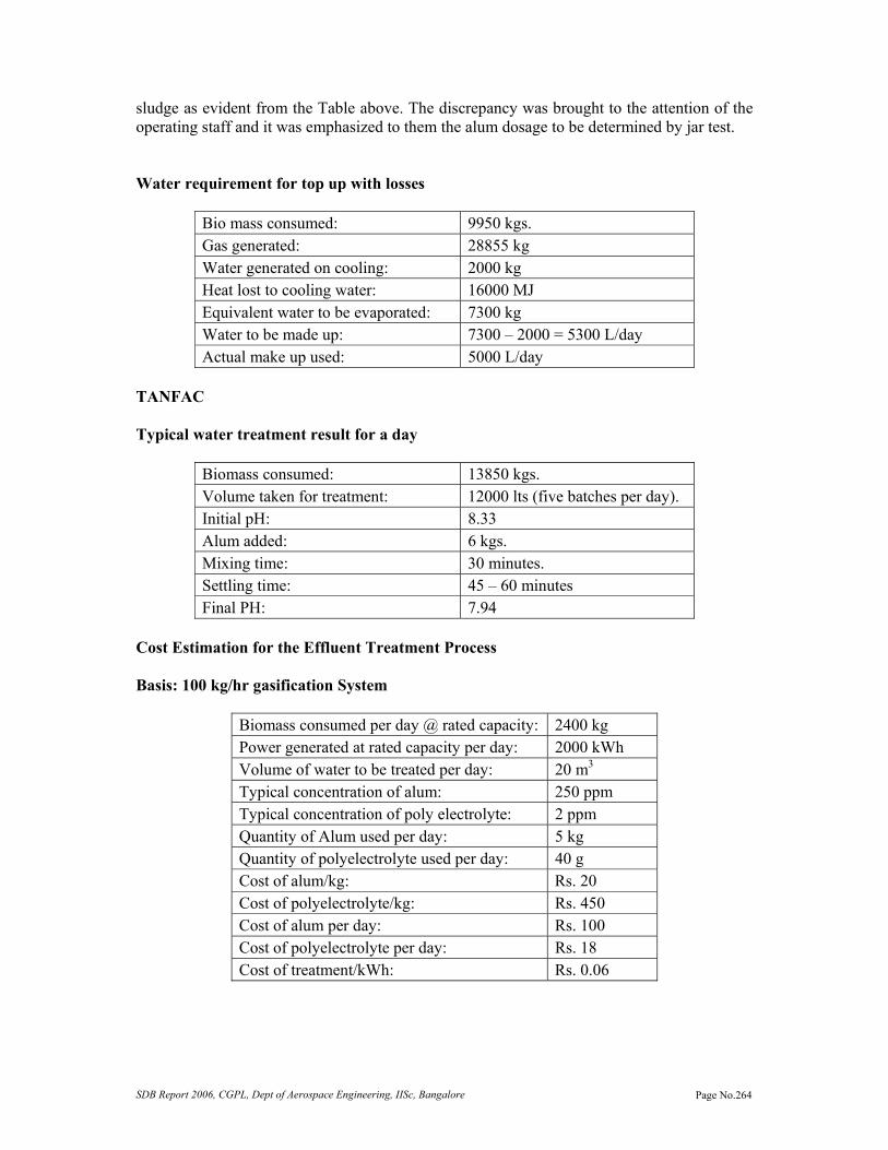
SDB Report 2006, CGPL, Dept of Aerospace Engineering, IISc, Bangalore Page No.264
sludge as evident from the Table above. The discrepancy was brought to the attention of the operating staff and it was emphasized to them the alum dosage to be determined by jar test. Water requirement for top up with losses
Bio mass consumed: 9950 kgs. Gas generated: 28855 kg Water generated on cooling: 2000 kg Heat lost to cooling water: 16000 MJ Equivalent water to be evaporated: 7300 kg Water to be made up: 7300 – 2000 = 5300 L/day Actual make up used: 5000 L/day
TANFAC Typical water treatment result for a day
Biomass consumed: 13850 kgs. Volume taken for treatment: 12000 lts (five batches per day). Initial pH: 8.33 Alum added: 6 kgs. Mixing time: 30 minutes. Settling time: 45 – 60 minutes Final PH: 7.94
Cost Estimation for the Effluent Treatment Process Basis: 100 kg/hr gasification System
Biomass consumed per day @ rated capacity: 2400 kg Power generated at rated capacity per day: 2000 kWh Volume of water to be treated per day: 20 m3 Typical concentration of alum: 250 ppm Typical concentration of poly electrolyte: 2 ppm Quantity of Alum used per day: 5 kg Quantity of polyelectrolyte used per day: 40 g Cost of alum/kg: Rs. 20 Cost of polyelectrolyte/kg: Rs. 450 Cost of alum per day: Rs. 100 Cost of polyelectrolyte per day: Rs. 18 Cost of treatment/kWh: Rs. 0.06