detection of circulating tumor cells in samples from...
TRANSCRIPT
Detection of circulating tumor cells in
samples from colorectal cancer patients using
digital fluorescent microscopy and image
cytometry
PhD thesis
Viktor Sebestyén Varga M.Sc.
Semmelweis University, II. Department of Internal Medicine
Semmelweis University, School of PhD Studies
Clinical Medicine Doctoral School Gastroenterology PhD
program
Program leader and supervisor: Prof. Tulassay Zsolt MD, DSc
Hivatalos bírálók:
Szigorlati bizottság elnöke:
Szigorlati bizottság tagjai
Budapest
2009
2
TABLE OF CONTENTS
TABLE OF CONTENTS ................................................................................................. 2
ABBREVIATIONS .......................................................................................................... 4 INTRODUCTION ............................................................................................................ 6 AIMS .............................................................................................................................. 10 METHODS ..................................................................................................................... 11
Scanning Fluorescent Microscopy.............................................................................. 11 Sample preparation ................................................................................................. 11 Scanning Fluorescent Microscope Hardware ......................................................... 11
SFM Software components .................................................................................... 12
Comparison of SFM, FCM and LSC .......................................................................... 18 High concentration samples for relative cell frequency determination .................. 18 Low concentration samples for absolute cell frequency determinations (SBC
measurements) ........................................................................................................ 19 Flow cytometry ....................................................................................................... 20
Laser scanning cytometry ....................................................................................... 20
Scanning fluorescent microscopy ........................................................................... 20 Visual Fluorescent microscopy analysis of rare cells ............................................. 22 Statistical analysis .................................................................................................. 22
Quantitative and stoichiometric fluorescent whole slide imaging.............................. 22 Samples ................................................................................................................... 22
Hardware ................................................................................................................ 24 Software development tools ................................................................................... 25
Algorithms .............................................................................................................. 25 Sample detection and localization .......................................................................... 25
Sample mapping ..................................................................................................... 26 Focusing ................................................................................................................. 26 Sharpness calculation ............................................................................................. 29
Image compensation ............................................................................................... 29 Digital gain ............................................................................................................. 30
Image segmentation ................................................................................................ 31 Quantitative and stoichiometric measurement ....................................................... 31
System linearity measurement ................................................................................ 31
Fluorescent digital slide .......................................................................................... 32
Fluorescent virtual microscopy .............................................................................. 32 Measurement evaluation tools ................................................................................ 34
RESULTS ....................................................................................................................... 35 Scanning Fluorescent Microscopy.............................................................................. 35 Comparison of SFM, FCM and LSC .......................................................................... 40
High concentration samples for relative cell frequency determination by FCM and
SBC measurements ................................................................................................. 41 Low concentration samples for absolute cell frequency determinations (SBC
measurements) ........................................................................................................ 43 Quantitative and stoichiometric fluorescent whole slide imaging.............................. 44
Focusing ................................................................................................................. 44
Scanning results ...................................................................................................... 45

3
Measurements: System stoichiometric linearity after compensation ..................... 46
DISCUSSION ................................................................................................................. 50 Scanning Fluorescent Microscopy.............................................................................. 50 Comparison of SFM, FCM and LSC .......................................................................... 54 Quantitative and stoichiometric fluorescent whole slide imaging.............................. 56
Sample detection and localization .......................................................................... 56
Automatic focusing ................................................................................................ 57 Quantitative imaging .............................................................................................. 59 Advancements over SFM ....................................................................................... 61
CONCLUSION .............................................................................................................. 63 SUMMARY ................................................................................................................... 64
ÖSSZEFOGLALÓ ......................................................................................................... 65 LITERATURE CITED ................................................................................................... 66 PUBLICATIONS’ LIST ................................................................................................ 73
ACKNOWLEDGEMENTS ........................................................................................... 79
4
ABBREVIATIONS
BP Band pass
CAM 5.2 Cell adhesion molecule
CCD Charge coupled device
CD45 Leukocyte common antigen
CV Coefficient of variation
DAPI 4',6-diamidino-2-phenylindole
DIC Differential interference contrast
DLL Dynamic Linked Libraries
DNA Deoxyribonucleic acid
DVD Digital Versatile Disc
ECDTM
R Phycoerythrin-Texas Red®-X
EDTA Ethylene diamine tetraacetic acid
FCM Flow cytometry
FCS Flow Cytometry Standard
FISH Fluorescent In-Situ Hybridization
FITC Fluorescein isothiocyanate
GB Gigabyte
HBO A part number commonly used to refer to mercury-vapor lamps
HDD Hard disk drive
HE High efficiency
HEA-125 Human epithelial antigen
HT29 Human colon adenocarcinoma grade II cell line
IF Integrated Fluorescence
JPEG Joint Picture Expert Group
LED Light emitting Diode
LP Long pass
LSC Laser scaning cytometry
MB Megabyte

5
NA Numerical aperture
NK cell Natural killer cell
PBS Phosphate buffered saline
PBMC Peripheral blood mononuclear cell
PC Personal Computer
PE Phycoerythrin
PMMA Polymethylmethacrylate
RAM Random Access Memory
RNA Ribonucleic acid
RPM Rotation per minute
RPMI 1640 Cell culture media
RT-PCR Reverse transcription polymerase chain reaction
SBC Slide based cytometry
SD Standard deviation
SFM Scanning Fluorescent Microscopy
SPF Synthesis-phase fraction
TDI Time-delay-and-integration
TOTO®
-3 Carbocyanine dimer, a red fluorescence stain that is a useful
counterstain
WSI Whole Slide Imaging
6
INTRODUCTION
In the last decades there has been a growing demand for multi-parametric quantitative
characterization of clinical and biological samples (1). Fluorescent assays have the
highest versatility for these purposes. There are many fluorescent dyes with different
excitation and emission characteristics and comparable biological specificity. These
facts make it possible to create multiple staining and use different filter combinations to
analyze cells. Recently enhanced focus is set on the rare cells of the human organ
(circulating tumor cells, physiologic and pathologic stem cells, fetal cells) (1, 2, 3).
Circulating tumor cells can be detected in peripheral blood samples by polymerase
chain reaction (PCR) or cytometry. PCR techniques require simpler sample handling
and instrumentation but they cannot provide morphological information as cytometry.
Rare cells have a frequency of 10-6
to 10-9
compared to the red and white blood cells in
the peripheral blood. The sensitivity of detection methods can be increased by
immunomagnetic cell enrichment. There are two major types of the immunomagnetic
sorting systems. The first one is using 2–5 µm magnetic beads with several hundreds or
thousands of antibodies on the bead surface. The second one is using supermagnetic
nanobeads bound to antibodies. In both systems the beads are bound to the cells of
interest and are separated from the rest by strong magnetic field. This technique
enriches the cells by 3-4 orders of magnitude.
The PCR technique developed in 1984 amplifies a few copy of DNA by several orders
of magnitude by thermo cycling. During the heating and cooling process the DNA is
going through a repeated denaturation and enzymatic replication cycle. The amplified
product is fluorescently labeled and separated from other DNA fractions by
electrophoresis in gel or capillaries. For the detection of circulating tumor cells Reverse
Transcription PCR (RT-PCR) is used. With this technique the RNA expressed
specifically by the tumor or other rare cells is transcribed back to DNA by reverse
transcriptase and the resulting DNA is amplified by the chain reaction. The PCR
process destroys the cells and their morphological analysis, re-staining, further

7
processing by other methods and the evaluation of their appearance in clusters becomes
impossible.
The two main cytometry approaches are flow and image cytometry and the first
experiments were made with both techniques approximately in the same time in the
1950s (4, 5).
In a Flow Cytometer, the cells flow through a laser beam in suspension. The laser beam
excites the fluorescent dyes and the emitted light is collected by photomultipliers. The
photomultiplier after amplification, pulse processing and, analog to digital conversion
provides the measured data to a computer. This data can be immediately analyzed and
stored. Flow cytometers can use arc lamps as well, but most commercial instruments
use one or more lasers.
Slide based image cytometers are built around microscope optics with fluorescent light
path and high resolution imaging capability. They provide similar data as FCM by
digitally processing the cell images.
Today flow cytometry (FCM) is used dominantly because it provides an easier
workflow and sample preparation; it has much higher throughput and due to its lower
complexity, its cost is lower. FCM can analyze 10,000 to 100,000 (6) cells per second in
comparison of slide based image cytometry’s (SBC) 100-1000 (1, 7). In SBC
measurements specimen position, outline and focus on the microscope slide has to be
determined precisely, which slows the workflow even further.
FCM has drawbacks too. For reliable subpopulation identification hundreds of cells are
necessary and its sensitivity is unsatisfactory for circulating tumor cell detection (8). For
the detection of circulating tumor cells slide based image cytometry (SBC) has several
advantages over FCM. It provides morphological and sub-cellular information. Cell
location on the slide is recorded and based on the measured data selected cells can be
relocated or examined with different imaging techniques. SBC can be utilized for
relatively small specimens and its application for rare cell detection is proven (7, 9).
Samples can be re-stained and rescanned to acquire more parameters and the analysis of

8
cell clusters and tissue is also possible (7, 10, 11). SBC lacks cell sorting capability but
there are attempts to overcome this limitation (12).
The development of computer and CCD (charge coupled device) camera technology
made possible about 20 years ago the appearance of slide based imaging cytometer
systems with acceptable throughput and data handling capability (13-17). Since that
time systems were developed based on Laser Scanning Cytometry (LSC) (7, 18-20),
standard (21-23), enhanced wide-field (1, 24-27) and confocal fluorescent microscopes
(10, 11, 28).
LSC is the most widespread SBC solution. It uses lasers to scan a slide in a similar
fashion as a confocal laser scanning microscope. This solution provides good results
because the laser spot has equal intensity on every location of the field of view and the
resolution is good. This technology developed by Compucyte Corp. (Westwood, MA) is
not confocal on purpose to collect fluorescence from the full depth of field. It has
medium throughput and it is expensive due to the lasers and laser beam scanning
mechanics.
Ecker et al. (10, 11, 28) developed a confocal microscope based tissue cytometer.
Tissue samples can be better segmented using the confocal technique because it images
only a thin layer of the specimen in contrast with LSC and the cells don’t overlap on the
recorded images. On the other hand fluorescence is not collected from the full depth of
field therefore precision and throughput is low and confocal microscopes are the most
expensive modalities for image cytometry.
Q3DM (San Diego, CA) enhanced a wide-field fluorescent microscope with phase-
contrast based focusing together with high speed electronics and stabilized mercury arc
lamp to increase imaging speed and quality (1, 24, 25). The core group of former
Q3DM developed recently a differential interference contrast (DIC) autofocus system
(26) for fluorescence microscopy and a volume camera based fast autofocus system for
a continuous-scanning automated microscope (27).

9
For clinical use standard fluorescent microscopes are the most promising modalities.
They are widely available; they have lower basic costs as other systems and they can be
used for general microscopic work which lowers the costs of circulating tumor cell
detection even further because no dedicated system is necessary.
The first attempts were made in the late 1980’s and 1990’s to convert the fluorescent
microscope into a scanner for single (16, 21) and multi-fluorescence measurements.
One of the first studies was published by Galbraith et al (14, 15). In their study they
showed, that multicolor fluorescence analysis can be performed by motorized
fluorescent microscopes. A comparison between flow cytometry and imaging cytometry
showed similar distribution of monocyte and NK cells from peripheral blood.
Kozubek et al. (29) developed the high-resolution cytometry, that enables automated
acquisition and analysis of fluorescent in-situ hybridization stained nuclei by wide-field
and confocal imaging techniques. Automated FISH analysis was also developed by
others (13, 30, 31). Mehes et al. has developed systems dedicated for rare cell detection
(32).
However in all of these cases, measurements are performed directly after image capture.
Only measured parameters and selected images are stored for later evaluation.
In the recent years another imaging microscopy field developed very rapidly.
Brightfield virtual microscopy or whole slide imaging (WSI) – the naming convention
is not consistent yet – became commercially available and starts to be established in
pathology (33-35). Whole slide imaging means that complete sections, cytospins and
smears can be digitized automatically in high resolution that is appropriate for
diagnosis. On the market currently there are two systems that are capable of fluorescent
WSI, the MIRAX SCAN and MIDI from 3DHISTECH (3DHISTECH Ltd., Budapest,
Hungary) and Carl Zeiss and the Hamamatsu Nanozoomer (Hamamatsu Photonics
K.K., Japan). The MIRAX system utilizes area cameras and is capable to digitize a
sample up to 9 channels. The NanoZoomer uses a time-delay-and-integration CCD
camera (TDI) and is capable to scan up to 3 channels.

10
AIMS
The objectives were as follows:
1. The development of methods to use a fluorescent microscope for quantitative
and stoichiometric cytometric measurements. This set of methods and software
is called Scanning Fluorescent Microscopy (SFM).
2. To show on biological samples that SFM is capable to reliably detect rare cells.
This is done by comparing the analytic accuracy of the developed SFM methods
with FCM and LSC on high and low cell concentrations (between 1:1 to 1:107
cell frequency) in artificial and clinical specimens.
3. The further development of the SFM methods to modify a fluorescent whole
slide imager to be capable of quantitative and stoichiometric measurements to
make the workflow effective enough for the clinical routine screening of
colorectal cancer patients.

11
METHODS
Scanning Fluorescent Microscopy
Sample preparation
For testing and calibration of the system, 10 µm diameter cytometric calibration beads
were used (Immuno-Brite Fluorospheres, Part No. 6603473, Beckman Coulter, Inc.,
Fullerton, CA). These beads had the advantage of being a mixture of populations, each
with an exponentially increasing number of fluorescent molecules.
For evaluation of clinical samples, residual samples from young, cancer free patients
were used. Mononuclear cells were isolated from EDTA anti-coagulated blood with
standard density gradient centrifugation (Histopaque-1077, Sigma-Aldrich Co., St.
Louis, MO). After removal of mononuclear cells from the layer floating on the
Histopaque, the cells were washed 3 times by PBS and counted in a Buerker chamber.
Ten µL of the cell suspension was smeared on microscope slide and dried. Cells were
stained in 100 nanomolar Hoechst 33258 for 20 min and washed in PBS. ProLong
Antifade (Invitrogen Corp., Carlsbad, CA) was used, as recommended by the
manufacturer, on dry smears to minimize fluorescent fading and permit multiple
scanning.
For the correction of mercury arc lamp uniformity errors, a slide with evenly distributed
FITC stain was prepared. 1mg / ml FITC solution was mixed with ProLong in 1:10
dilution and 30µl were applied to glass slide and covered with a 22mm * 22mm
coverslip.
Scanning Fluorescent Microscope Hardware
The SFM includes hardware and software components. In this study an Axioplan 2
imaging MOT (motorized) microscope (Carl Zeiss MicroImaging GmbH, Jena,
Germany) was used with motorized objective and filter changer. A Plan-Neofluar 20x,
0.5 NA dry objective was used for every scan in this study. The system was equipped
with a high resolution AxioCam HR color camera. Though the highest resolution of the
camera is 3900 * 3000 pixel with 14-bit depth, only 650 * 515 pixel resolution was used

12
with 8-bit depth in black and white mode. The relatively low resolution and bit depth
was used to lower the exposure time as much as possible in order to speed up scanning.
The software ran on a 700MHz PIII PC with 256 MB of RAM and 40 GB HDD. The
operating system was Microsoft Windows NT Workstation 4.0 with service pack 6
(Microsoft Corp., Redmond, WA). The image acquisition required only the PC interface
card provided with the AxioCam. The microscope was controlled through the RS-232
port of the computer. The microscope and camera were controlled using the software
libraries provided by Carl Zeiss. SFM will work with any PC with the above or better
characteristics.
SFM Software components
I developed the SFM software components in C++, using C++Builder (Embarcadero
Technologies, San Francisco, CA). Figure 1 is a flow chart that describes their
interactions.

13
Figure 1. Flow chart of the working logistics with the SFM Program. Following the
arrows one can see the steps of scanning or evaluating a slide.
Hardware handling modules:
These modules are Dynamic Linked Libraries (DLL), like all the others, and contain a
low but abstract level of functions to control the specific hardware to which they
belong.
Scanning module:
This is a complex module, which unites other smaller modules. This module covers the
complete functionality of scanning. It contains the following modules: settings, image-
processing, scanning strategy and scanning area designation. The scanning strategy
module can be changed to realize different scanning approaches.
START
END
SLIDE HANDLING, SCANNING, SETTINGS,
EXIT
DISPLAYING SLIDE WITH
VIRTUAL MICROSCOPE
IMAGE PROCESSING
RESULT EXISTS?
EVALUATION USING SCATTER PLOT,
FREQUENCY HISTOGRAM,
GALLERY
REPORT
PSEUDO COLORING, THRESHOLD SETTING,
IMAGE PROCESSING
MANUAL SLIDE
INSERTION
SCANNING AREA
DESIGNATION
AUTOMATED SCANNING,
STORING THE COMPLETE SLIDE
MANUAL SLIDE
REMOVAL
MICROSCOPE SETTINGS,
LOAD/STORE
STAGE SETTINGS,
LOAD/STORE
CAMERA SETTINGS,
LOAD/STORE
14
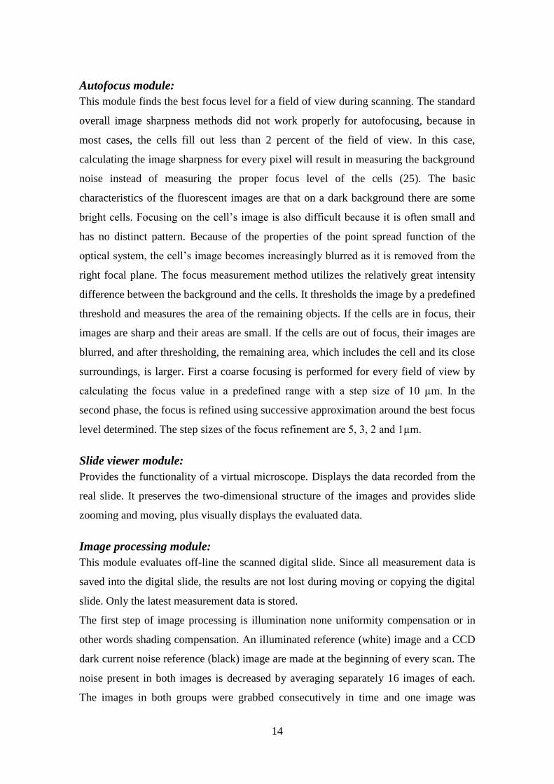
Autofocus module:
This module finds the best focus level for a field of view during scanning. The standard
overall image sharpness methods did not work properly for autofocusing, because in
most cases, the cells fill out less than 2 percent of the field of view. In this case,
calculating the image sharpness for every pixel will result in measuring the background
noise instead of measuring the proper focus level of the cells (25). The basic
characteristics of the fluorescent images are that on a dark background there are some
bright cells. Focusing on the cell’s image is also difficult because it is often small and
has no distinct pattern. Because of the properties of the point spread function of the
optical system, the cell’s image becomes increasingly blurred as it is removed from the
right focal plane. The focus measurement method utilizes the relatively great intensity
difference between the background and the cells. It thresholds the image by a predefined
threshold and measures the area of the remaining objects. If the cells are in focus, their
images are sharp and their areas are small. If the cells are out of focus, their images are
blurred, and after thresholding, the remaining area, which includes the cell and its close
surroundings, is larger. First a coarse focusing is performed for every field of view by
calculating the focus value in a predefined range with a step size of 10 µm. In the
second phase, the focus is refined using successive approximation around the best focus
level determined. The step sizes of the focus refinement are 5, 3, 2 and 1µm.
Slide viewer module:
Provides the functionality of a virtual microscope. Displays the data recorded from the
real slide. It preserves the two-dimensional structure of the images and provides slide
zooming and moving, plus visually displays the evaluated data.
Image processing module:
This module evaluates off-line the scanned digital slide. Since all measurement data is
saved into the digital slide, the results are not lost during moving or copying the digital
slide. Only the latest measurement data is stored.
The first step of image processing is illumination none uniformity compensation or in
other words shading compensation. An illuminated reference (white) image and a CCD
dark current noise reference (black) image are made at the beginning of every scan. The
noise present in both images is decreased by averaging separately 16 images of each.
The images in both groups were grabbed consecutively in time and one image was

15
made by averaging the same pixel in every image. The white reference image is made
using the evenly spread FITC slide described in the sample preparation section. The
black reference image is made by closing the camera shutter on the microscope. The
black reference image is for compensating the dark current error of the camera. The
black reference image is subtracted from every image because it represents the standard
error of the camera. Every field of view is compensated according to the following
equation, Eq. 1.a. I’ denotes the compensated image, I denotes the original, B the black
reference and W the white reference image. The x and y indices denote a pixel of the
images, u and v denotes the co-ordinates of the brightest pixel in the white reference
image.
Eq. 1.a. yxyx
vu
yxyxyxBW
BWBII
vu
,,
,max
,,,
,)(
The following example explains how compensation works. In Eq. 1.a., the
corresponding pixel value of the black compensation image is subtracted from every
pixel value. In our example, we suppose that the camera is ideal and has no dark current
error. In case of modern Peltier cooled CCD cameras, this is almost true and the black
reference image has gray level pixel values less than 3. If we eliminate black reference
subtraction from Eq. 1.a., we get Eq. 1.b.
Eq. 1.b. y,x
maxy,xy,x
W
WII
Figure 2A represents a white compensation image; the 9 regions of the image are
illuminated with different intensities. The gray level values of the pixels in a region are
written in the region. Figure 2B represents one field of view with beads of equal amount
of fluorescent molecules; each bead’s gray level value is indicated next to it. For the
ideal case of even illumination, the gray level values should be equal, but the values are
linearly proportional to illumination intensity.
Compensation works the following way. First, a search is performed for the gray level
value of the brightest region of the white reference image. This will be Wmax, 210 in the

16
example. Now we modify the gray level values of the beads. The gray level value of the
bead in the lower right corner of Figure 2B is 77, this will be Ix,y in equation 1.b. The
gray level value of this bead’s region in the white reference image is 70, this will be
Wx,y. If these values are substituted to equation 1.b. the result I’x,y will be 231. Equation
1.c. demonstrates the calculation.
Eq. 1.c. 70
21077231
Figure 2C represents the compensated field of view. Unlike in the example, in SFM the
compensation is done per pixel and not per bead.
Figure 2. Artificial images demonstrating shading correction on one field of view. A: Demonstration white compensation image. The nine regions represent the different
illuminations. Numbers in regions show the gray level values. B: Demonstration of
uncompensated field of view. The beads should have the same brightness but they are
different because of the uneven illumination. Beads’ gray level values are shown beside
them. C: Same demonstration field of view as in b. after compensation, beads have the
same intensity. Beads’ gray level values are shown beside them.
17
In the second step of image processing, images are thresholded. Every channel has a
separate threshold value. If the blobs remaining after threshold have overlapping pixels
in the different channels, their union is treated as a cell.
The following morphometric parameters are calculated for every cell: maximum
diameter, minimum diameter, average diameter, area, and perimeter. The following
fluorescence parameters are calculated for every cell: integrated fluorescence, minimum
fluorescence, maximum fluorescence, average fluorescence, and fluorescence range.
Fluorescence in our terminology means the intensity of a pixel in the cell’s image.
Minimum fluorescence is the value of the darkest pixel, maximum fluorescence is the
value of the brightest pixel, average is the average of all the pixels, and range is the
difference between maximum and minimum.
Integrated fluorescence (IF) is the same as fluorescence in FCM. In equation 2., IF is
the integrated fluorescence of one cell in one channel. Ci is a pixel of the cell’s image
and B is the average value of the neighboring background pixels around the cell. Those
pixels are considered as a neighboring background pixel, whose graylevel value is
below the channel’s threshold and are within a rectangle. This rectangle’s edges are 5
pixels farther from the cell’s most left, right, top and bottom pixels. In other words, to
calculate the integrated fluorescence, from every pixel of the cell, the average
neighboring background value is subtracted and these results are summed.
Eq. 2. i
i )BC(IF
Cytometry evaluation module:
Scatter plots, histograms and galleries can be used for the evaluation of the data derived
from image processing. The SFM software can export data to an FCS file; however for
purposes of efficiency, we have implemented the functions of a standard FCS analysis
program to integrate the functions with the digital slide, galleries and Microsoft® Word
export.
The software handles a maximum of six fluorescent channels. For every channel, a
separate pseudocolor and image processing threshold can be defined manually. Any
parameter of each channel can be displayed on the x and y axis of a scatter plot or on

18
the x axis of a histogram. The gates can be linked, i.e. the cells defined by a gate on a
scatter plot can be the source data of a histogram and vice-versa. An arbitrary number of
gates can be linked and any gate’s data can be displayed in a gallery. If a cell is clicked
in the gallery the dot representing the cell will turn to red from black in every displayed
scatter plot and the digital slide is centered around the clicked cell, which is now
highlighted. The created scatter plots, histograms and galleries can be exported into a
Microsoft® Word document as an image and the cells’ data as a table.
The field of views in the digital slide were stored in standard JPEG format using Intel’s
Intel JPEG Library 1.5 (Intel, Corp., Santa Clara, CA).
The statistical analysis was performed by the Statistica program package (StatSoft, Inc.,
Tulsa, OK).
Comparison of SFM, FCM and LSC
High concentration samples for relative cell frequency determination
Peripheral blood mononuclear cells (PBMCs) were isolated from EDTA anti-coagulated
blood (from young cancer free patients after informed consent and approval of the
Ethical Committee of the Semmelweis University Budapest, Hungary) with a standard
density gradient centrifugation (Histopack 1.077). The isolated PBMCs were washed
three times in phosphate buffered saline pH=7.4 (PBS). HT29 tumor cells cultured in
RPMI 1640 (Sigma-Aldrich) supplemented with 10% fetal calf serum (Sigma-Aldrich)
were detached by 0.25% trypsin – 0.02% EDTA solution (T4049, Sigma-Aldrich) and
washed three times in PBS.
HT29 and PBMCs cells were counted manually with a hemocytometer and mixed at
different ratios (HT29 to PBMC ratios: 1:1, 1:2, 1:4, 1:8, 1:20, 1:50, 1:100, 1:500,
1:1,000) in three replicates. 100,000 – 200,000 cells in 50 - 100 l were used per
mixture. 5 l anti human CD45 ECD (PE-TexasRed tandem dye) (Beckman Coulter –
Immunotech, Krefeld, Germany) and 5 l CAM 5.2-FITC (Becton Dickinson
Immunocytometry Systems (BDIS), San Jose, CA) antibodies were added and
incubated 30 min in the dark at room temperature. After 2x washing in PBS by
centrifugation at 1,500 RPM (5 min, Janetzki T32), the cells were fixed for 20 min in

19
0.5 % phosphate buffered paraformaldehyde. Cells were pelleted, and the supernatant
was discarded. Then the cell were resuspended in the remaining 100 l solution. The
DNA specific fluorescent dyes TOTO-3 (Invitrogen) in 5 M final concentration and
Hoechst 33258 (Invitrogen) in 100 nM final concentration in PBS were added and cells
were stained for 20 min, in the dark at room temperature. Cells were then washed in
PBS, supernatant was discarded. Then samples were divided into two parts for FCM
and SBC measurements, respectively.
From 10 l of the resuspended pellet, smears were placed onto a spot with a diameter of
5- 6 mm in the middle of conventional glass slide. Smears were covered by the ProLong
antifading agent (Invitrogen). It was used as recommended by the manufacturer on dry
smears to stabilize the fluorescent signal for long time and permit multiple scanning.
The same slides were used for SFM and LSC measurements.
Low concentration samples for absolute cell frequency determinations
(SBC measurements)
Slides prepared by micromanipulation of tumor cells from tissue culture
Histopack 1.077 separated mononuclear cells were CD45 ECD labeled with the above
protocol, smeared in the middle of the slide and dried. From a CAM5.2 labeled HT29
cell suspension cells were sucked up and dropped on the slide among leukocytes by a
micro-manipulator (Carl Zeiss) under fluorescent microscopy control. The number of
HT29 cells placed on the slide was visually counted (5-50 cells were placed on a slide).
The same slides were used for SFM and LSC measurements.
Slides prepared from the blood of tumor bearing patients
In another experiment peripheral blood of colorectal cancer patients with different
Dukes stages (B:2, C:3, D:5) were evaluated by the standard protocol (Miltenyi Biotech,
Bergisch Gladbach, Germany). Shortly, mononuclear white blood cells and circulating
tumor cells were isolated from 20 ml EDTA anti-coagulated peripheral blood by a
standard density gradient centrifugation (Histopack 1.077). Cells were washed 3 times

20
by PBS and labeled with the anti-human epithelial antigen (HEA-125) magnetic
microbead conjugated antibody (Miltenyi Biotech, Bergisch Gladbach, Germany) with
FCR blocking reagents (Miltenyi Biotech). Enrichment of HEA-125 expressing tumor
cells was achieved using MS cell separation columns (Miltenyi Biotech). After isolation
in the magnetic field (MiniMacs, Miltenyi Biotech) the enriched cell fractions were
labeled according to the above immuno-cytochemical labeling protocol for CD45 ECD,
CAM 5.2 FITC, and nuclear DNA. After washing cells were cytocentrifuged
(STATSPIN E802/22 centrifuge at 700 RPM, 10 min) on the slide. After air-drying
cells were covered with ProLong medium. The identical slides were used for SFM and
LSC measurements.
Flow cytometry
The leukocyte and the HT29 cell suspensions were filtered through 50µm nylon mesh
(Partec GmbH, Münster, Germany). The analysis was performed on a FACScan flow
cytometer (BDIS), equipped with a Macintosh Quadra 650 computer and CellQuest
software. 488 nm argon-ion laser excitation at 15 mW was used. With FSC triggering
the fluorescence signals were detected at 530+15 nm Bandpass (BP) filter (FITC) and
650 nm Long pass (LP) filter (ECD). 10,000-15,000 cells were measured, per sample.
Laser scanning cytometry
LSC (Compucyte) was equipped with a 20x UPLANFL (Universal plan Semi-
apochromatic) NA-0.5 objective (Olympus). Fluorochromes were excited by a 488 nm
argon-ion (5 mW) and a 633 nm HeNe (5 mW) laser and fluorescence signals detected
at 530 / 30 nm BP (FITC), 625 / 28 nm BP (ECD) and 670 / 20 nm BP (TOTO-3)
filters. The TOTO-3 signal was used for triggering.
Scanning fluorescent microscopy
The Hoechst 33258 fluorescence signal (with the strongest fluorescent light) was used
for focusing. An entire smear area or at least 1,000 cells were scanned automatically at

21
20x magnification. Scanning sequence was Hoechst 33258, ECD, FITC. Fluorescent
light was detected for Hoechst 33258 with Zeiss filter set 02, for ECD staining with
Zeiss filter set 20 and for FITC Zeiss filter set 10.
The digitization times for the single field of views were different in the three channels
depended on the strength of the fluorescent signals (100 ms for Hoechst 33258, 1000 ms
for ECD and 400 ms for FITC). The spatial resolution of the system was 0.645 m /
pixel.
The digital slide was evaluated using virtual microscopy and standard cytometry
techniques (Figure 3).
Figure 3. Steps of the image data analysis by the SFM program. A: A virtual
microscopy evaluation field in the multi-channel digital slide made by the SFM showing a
clinical sample for rare cell detection. Of the six available channels, 3 are used. One is
applied for Hoechst 33258 channel, the second for ECD, the third for FITC. Magnification
is 100x. A single CAM 5.2 positive cell is shown in the middle (arrow), it is surrounded by
CD45 positive cells. B: Cell recognition by SFM, found objects are indicated by a circle.
C: quantitative data of cells generated by the image analysis of multi-channel digital slide
could be analyzed by SFM as standard cytometric results. In the scatter plot FITC positive
rare tumor cells are gated. The X axis shows the ECD channel intensity, the Y axis is the
FITC channel intensity value. Six cells are located inside the gate. (Arrow indicates a point
on the dot plot which represents a cell that was relocated on 3A.) D: Gallery of the six
gated tumor cells with electric pseudomagnification. The Hoechst 33258 stained nuclei and
the CAM5.2-FITC labeled surface are clearly visible. The highlighted cell (arrow) in the
cell gallery window is shown by the SFM in 3A.
B
C D
A

22
Visual Fluorescent microscopy analysis of rare cells
The manual screening and evaluation of low concentration specimens was performed by
two independent observers using an AxioPlan 2 Imaging microscope equipped with
triple path and single path filters for FITC, ECD and Hoechst 33258 staining and an
Axiocam camera. The images of the single cells were recorded with the positions using
the AxioVision software (V.3.0, Carl Zeiss ImagingSolutions GmbH, Munich,
Germany).
Statistical analysis
The statistical analysis (linear regression, determination of correlation coefficients) was
done using the Sigmaplot and SPSS program (SPSS V.8.0 Knowledge Dynamics
Canyon Lake, USA).
Quantitative and stoichiometric fluorescent whole slide imaging
Samples
For testing and calibration of the system the same cytometric calibration beads were
used as for SFM. For evaluation of clinical samples, residual samples from young,
cancer-free patients were prepared in the same way as for SFM. Mononuclear cells were
isolated from EDTA anti-coagulated blood with standard density gradient centrifugation
(Histopaque-1077). After removal of mononuclear cells from the layer floating on the
Histopaque, the cells were washed three times by PBS and counted in a Buerker
chamber. A total of 10 µl of the cell suspension was smeared on a microscope slide and
dried. Cells were stained in 100 nM Hoechst 33258 for 20 min, and washed in PBS.
As recommended by the manufacturer, ProLong Antifade (Invitrogen, Carlsbad, CA)
was used on dry smears to minimize fluorescent fading and permit multiple scanning.

23
For correction of the illumination uniformity errors, a special compensation slide was
prepared by the Fraunhofer Institute for Applied Optics and Precision Engineering IOF
(Jena, Germany). On a glass slide in a 1.45 µm thick polymethylmethacrylate (PMMA)
layer the following laser dyes were diluted (Radiant Dyes Laser & Accessories GmbH,
Wermelskirchen, Germany; article number, name, concentration in Mol/l): 044,
Coumarin 2 (C450), 3x10⁻³; 072, Coumarin 545, 1x10⁻⁴; 084, Rhodamine 6G (Rh590),
1x10⁻⁴; 087, Rhodamine 101 (Rhod640), 1x10⁻⁴; 102, Oxazin 4 (LD690 Perchl.),
1x10⁻⁴; 101, Nile Blue Perchl., 2x10⁻⁵; 119, Rhodamine 800 (LD800), 2x10⁻³.
24
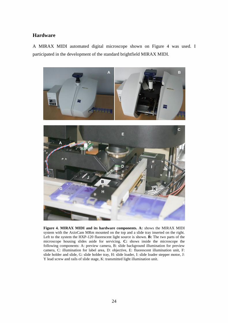
Hardware
A MIRAX MIDI automated digital microscope shown on Figure 4 was used. I
participated in the development of the standard brightfield MIRAX MIDI.
Figure 4. MIRAX MIDI and its hardware components. A: shows the MIRAX MIDI
system with the AxioCam MRm mounted on the top and a slide tray inserted on the right.
Left to the system the HXP-120 fluorescent light source is shown. B: The two parts of the
microscope housing slides aside for servicing. C: shows inside the microscope the
following components: A: preview camera, B: slide background illumination for preview
camera, C: illumination for label area, D: objective, E: fluorescent illumination unit, F:
slide holder and slide, G: slide holder tray, H: slide loader, I: slide loader stepper motor, J:
Y lead screw and rails of slide stage, K: transmitted light illumination unit.
B A
C

25
MIRAX MIDI can scan in brightfield and with our further development in fluorescence.
It has a slide loader mechanism for 12 slides and it has 200 µm focus range. The system
had a Carl Zeiss 20x Plan-Apochromat, NA 0.8 dry objective. Three high efficiency
Zeiss filter blocks were used for DAPI (Filter Set 49), FITC (Filter Set 46HE) and
Rhodamine (Filter set 43HE). For the quantitative fluorescent measurements a Carl
Zeiss Colibri LED light source was used with 365 nm and 470 nm LED modules. For
general scanning tests a Carl Zeiss HXP 120 metal-halid short arc lamp was used that
can be fiber coupled to the Colibri lamp. The illumination pathway was used from the
Zeiss AxioScope 40 and the microscope had a 10 position filter wheel. For image
capture a Zeiss AxioCam MRm Rev.3 monochrome camera was used. The camera has
1388 x 1040 pixels and 6.45 µm x 6.45 µm pixel size, 12 bit digitization, 17000
electrons full well capacity and single-stage Peltier-cooling. With the 20x objective one
pixel imaged a 0.3225 µm x 0.3225 µm area of the specimen.
The software ran on a PC with dual Intel Xeon 2.8 GHz processors, 2 GB RAM and 500
GB hard drive. The operating system was Microsoft Windows XP.
Software development tools
The software is an extension of the MIRAX SCAN control program developed in
Microsoft Visual Studio 6 and C++ Builder. For displaying the slides I used the MIRAX
Viewer digital slide viewer. I developed the here described sample detection, sample
mapping, focusing, sharpness calculation, image compensation and digital gain
functions. I participated in the development of the here described fluorescent digital file
format, virtual microscope and measurement evaluation tools. The HistoQuant module
used for evaluation is the development of my colleagues.
Algorithms
To digitize fluorescently labeled samples on a slide its location, focus position and
exposure time in every channel has to be determined.
Sample detection and localization

26
MIRAX MIDI is equipped with a preview camera to grab a low resolution image from
the slide to determine areas for imaging. This optical path has transmitted light
illumination and no epifluorescence. The sample is illuminated from the back by a light
emitting panel without additional optics (Figure 4C). Fluorescent samples have low
contrast in transmitted illumination mode and are not detectable by the preview camera.
To overcome this limitation the fluorescent imaging software requires to circle the
sample with a continuous line on the slide with a black marker pen.
Sample mapping
Before imaging the sample is mapped. On grid points the sample is focused and
exposure times are measured in every channel. The focus values are interpolated to
determine every field of view’s own focus level. In every channel the shortest grid point
exposure time is selected for scanning. The distance of the grid points can be set
manually in field of views. A typical value is 3.
Mapping time is shortened by limiting the full 200 µm focus range to 50 µm. The
algorithm goes through the grid points from the center of the scan area following a
spiral path. The focus level of the first field of view that contains sample will be the
middle of the limited range. A field of view is considered to contain sample if there are
values above column 50 in the pixel value difference histogram. The generation of the
histogram is described in the Sharpness calculation section.
Focusing
MIRAX MIDI has 200µm focus range. In fluorescent microscopy both excitation and
emitted lights are focused by the objective. As the fluorescent sample gets out of focus
its brightness decreases as shown on Figure 5.

27
Figure 5. Exposure time as a function of focus. In fluorescent microscopy the exposure
time strongly increases as the sample gets out of focus. To demonstrate this effect the
exposure time was calculated for a field of view with a single bead at different focus levels
throughout the focus range. At 76 µm Z position the exposure time was 9 ms and at 164 µm
732 ms.
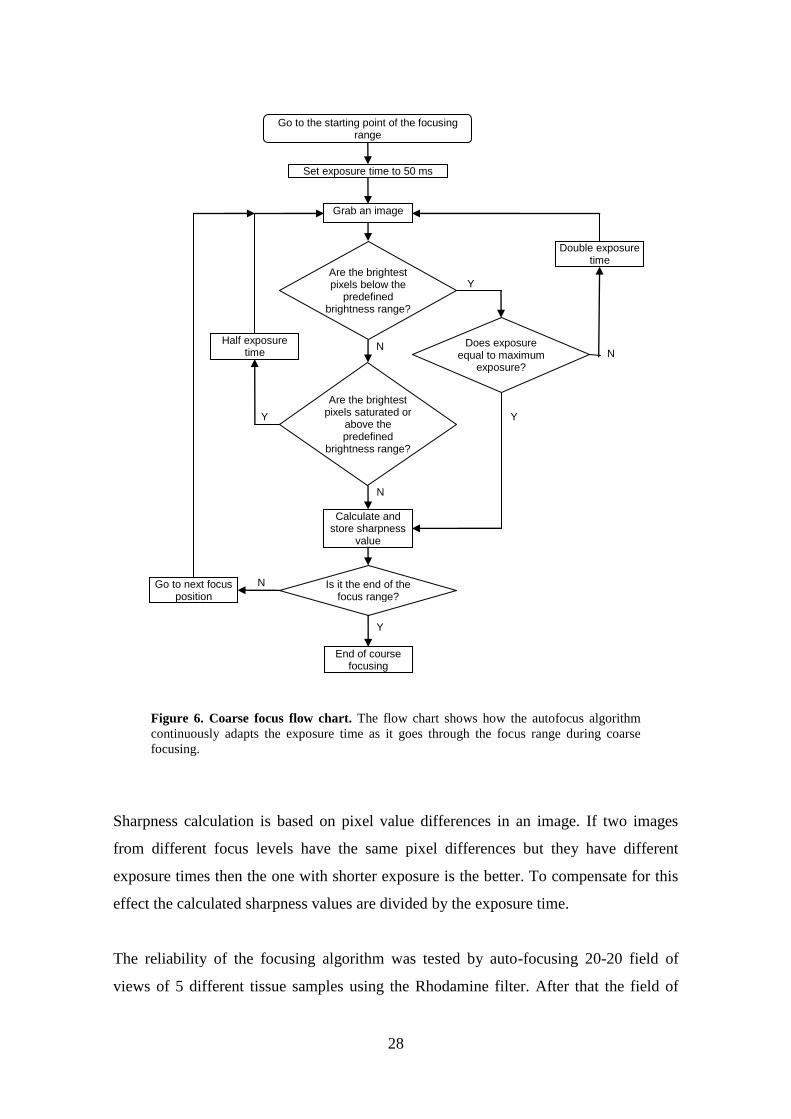
To adapt to the varying light intensity the exposure time is continuously adjusted during
focusing. An intensity range is defined and the algorithm keeps the brightest pixels
always in this. The bottom of the range has half the brightness as the top. In the
software three different ranges can be selected, from 32 to 63 which is the default, from
64 to 127 and from 128 to 255. The auto focus algorithm first goes through the whole
range in 4 µm steps and then fine focuses around the best position. Figure 6 shows the
flow chart of the coarse focus integrated with the continuous exposure change.
0 ms
100 ms
200 ms
300 ms
400 ms
500 ms
600 ms
700 ms
800 ms
0 50 100 150 200
Exp
osu
re t
ime
[m
s]
Focus level [µm]
28
Figure 6. Coarse focus flow chart. The flow chart shows how the autofocus algorithm
continuously adapts the exposure time as it goes through the focus range during coarse
focusing.
Sharpness calculation is based on pixel value differences in an image. If two images
from different focus levels have the same pixel differences but they have different
exposure times then the one with shorter exposure is the better. To compensate for this
effect the calculated sharpness values are divided by the exposure time.
The reliability of the focusing algorithm was tested by auto-focusing 20-20 field of
views of 5 different tissue samples using the Rhodamine filter. After that the field of
Go to the starting point of the focusing range
Grab an image
Set exposure time to 50 ms
Are the brightest pixels below the
predefined brightness range?
Double exposure time
Y
N
Are the brightest pixels saturated or
above the predefined
brightness range?
Half exposure time
Y
Calculate and store sharpness
value
Go to next focus position
Is it the end of the focus range?
N
Y
End of course focusing
N
Does exposure equal to maximum
exposure?
N
Y

29
views were fine focused again manually in 0.2 µm steps and the difference between the
manually and automatically determined focus values was calculated.
Sharpness calculation
Sharpness value calculation is based on a pixel value differences histogram. To lower
noise and small artifacts the field of view is shrunk by averaging 3.33 x 3.33 pixels.
From this image a pixel difference histogram is calculated. If the difference between a
pixel and its neighbor to the right is 10 then in the histogram column 10 is incremented
by 1. An image with 8 bit depth results a 256 (28) column histogram. After histogram
generation its values are multiplied with the 5th
power of the histogram indices. For
example the values of column 10 and 255 are multiplied by 100000 and
1078203909375 respectively. Sharpness value of the image is the sum of the column
values.
Image compensation
The field of view is not illuminated evenly by the light source. The Colibri and HXP-
120 lamps provides a more even illumination as conventional HBO mercury arc lamps
but this is still not sufficient for quantification. We measured 15% intensity difference
between the best and worst illuminated area. The fluorescence of the cells is measured
by the intensity of their pixels. Objects with equivalent fluorescence will show different
intensity depending on their position in the field of view and the illumination of that
area. This error is corrected by using a compensation image. Ten empty field of views
are recorded on random positions of the compensation slide in every channel. From the
10 images in every channel 1 final compensation image is created by omitting the
darkest and brightest pixels and averaging the rest in every pixel position. This method
eliminates local artifacts from the individual images which are usually darker or brighter
than the compensation slide itself. The averaging lowers the noise of the camera (36). In
the SFM system 16 images were recorded to lower the camera noise but they were
recorded on one location and the slide artifacts could not be eliminated.

30
During acquisition of the digital slide every image is compensated using the following
equation:
𝐼′𝑥𝑦 = 𝐼𝑥𝑦𝐶𝑚𝑎𝑥 𝑢𝑣
𝐶𝑥𝑦
I’ denotes the compensated image, I denotes the original image and C denotes the
compensation image. The x and y indices denote an image pixel, and u and v denote the
coordinates of the brightest pixel of the compensation image.
On the MIRAX system there is no shutter to close completely the light path to the
camera so no black compensation image was recorded and used as in the case of SFM.
To assess the black image of the camera it was removed from the microscope and its
aperture was closed by a C-mount cap. In 8 bit mode the black image had pixel values
of 1 which has negligible influence on measurement data if it is not included in the
compensation process. To make the display of digital slides faster the compensation is
done during scanning and not during slide display as in the SFM system.
To evaluate the effect of compensation 1200 of the brightest Coulter beads with 20 ms
exposure time were scanned without compensation and their CV value was compared to
the same bead population scanned with compensation for the system linearity
measurements detailed later.
Digital gain
The AxioCam MRm grabes 12 bit images but the MIRAX system handles only 8 bit
images. We implemented in the system a Digital Gain function which stores the user
selected 8 bit from the original 12. The default setting is digital gain 0 what means that
the most significant 8 bit will be stored and digital gain 4 means that the least
significant 8 bits will be stored. This way the user can select between scanning speed
and image noise. Every step of the digital gain halves the exposure time but increases
the noise. The recommended setting for standard imaging is digital gain 2 because the
exposure times are 4 times shorter and the increase in noise is hardly noticeable. For the
quantitative measurements digital gain 0 was used.

31
Image segmentation
The system uses thresholding for image segmentation. For a segmentation an upper and
lower threshold can be defined and pixel values below and above those values will be
excluded. Neighboring pixels are grouped to one object. Within one measurement
several segmentations can be included and all of them are displayed by user selected
colors on the digital slide. Before segmentation the image can be filtered by Gauss,
Median or Wiener filter with a kernel size of 0-10 pixels. 0 means that the filtering is
off. The filter algorithms are implemented in the Intel Integrated Performance
Primitives image processing package (Intel Corp., Santa Clara, CA). The actual image
processing is done on the original pixel data, filtering is used only for segmentation.
Detected objects can be further filtered based on their size in µm2. Segmentation
settings can be saved as a Mirax Image Segmentation Profile file with .misp extension.
Quantitative and stoichiometric measurement
The following parameters are measured for each object: area, perimeter, shortest and
longest diameter, shape factor, average pixel intensity and integrated fluorescence (IF).
Shape factor is calculated with the following equation:
𝑆𝐹 =4 × 𝛱 × 𝑎𝑟𝑒𝑎
𝑝𝑒𝑟𝑖𝑚𝑒𝑡𝑒𝑟2
The shape factor is 1 if an object is perfectly round. IF has the same function as
fluorescence in FCM. From every pixel the average value of the background around the
object is subtracted and the pixel values are summed as in the SFM system. Area,
perimeter and diameters are measured in µm. The system automatically calculates the
µm/pixel value from camera type, objective magnification and camera adapter
magnification. This value is stored in the digital slide and can’t be modified.
System linearity measurement
32
The system’s linearity was verified by three different methods. To measure exposure
linearity 1000 beads from the brightest population were scanned with 5, 10, 15, 20 and
25 ms exposure time. To test single exposure linearity 1800 beads were scanned at once
from a mixture of all the 5 intensities. The IF of the different populations was
compared to the manufacturer supplied intensity data. In both cases from the measured
objects the clustered beads were filtered.
To verify areal linearity 5300 beads and bead clusters from the 3rd
intensity were
scanned and the IF of different cluster sizes was correlated.
Finally we measured the CV value of Hoechst stained lymphocytes to assess usability
on real samples.
Fluorescent digital slide
The standard proprietary file format of the MIRAX system was used to store the
fluorescent digital slides. This format stores the images in an overlapped tiled format at
10 different magnifications. Every magnification layer is the half of the previous one
starting from 1:1, 1:2 and down to 1:512. The storage of different magnifications is
necessary to provide fast magnification change in the viewer software. One image of the
camera is split to 4x4 smaller images because these can be handled more efficiently if
the digital slide is browsed on the Internet. Tiles can be stored internally in 3 different
user selectable image file formats: BMP (Bitmap), PNG (Portable Network Graphics) or
JPEG (Joint Picture Expert Group). The compression rate of the JPEG format can be
defined by the user. Three fluorescent channels are stored in the red, green and blue
channels of a standard color brightfield image. If more than three channels are scanned
then a new layer of RGB image is stored in the file. The format also stores the preview
image of the slide recorded by the preview camera and the label area image.
Fluorescent virtual microscopy
For slide display the MIRAX Viewer software was used. The viewer has the following
main functions: arbitrary magnification selection, panning, annotation handling,
measuring and opening slides from a teleconsultation server on the Internet.

33
Additionally several slides can be opened at the same time for comparisons, annotation
areas can be exported to reports, the viewer can be controlled from the keyboard for
faster handling and synchronized multiple participant teleconsultation sessions are also
possible. The viewer stores what areas of the slide were examined and at what
magnification for quality control. Above the basic viewer functions the fluorescent
slides can be used with application packages for tissue micro arrays, quantitative
measurement, education and three-dimensional reconstruction. The measurements in
this work were made with the HistoQuant package of the MIRAX family.
The viewer had to be modified to read more than one image layer in case more than
three channels are digitized. For every channel pseudo color, brightness, contrast and
gamma can be set individually. These controls are on the bottom of the viewing area on
Figure 7.
Figure 7. MIRAX Viewer. On the left side of the viewer window there are two previews.
The upper one always shows the complete slide area for navigation. The lower preview
shows a magnified image for better orientation. In the center is the main viewing area. In
the upper right corner there is a magnifier window showings the area around the mouse
cursor with 4 times higher magnification as the main working area. Fluorescent channels
selection, pseudo colorization, brightness, contrast and gamma settings are below the main
viewing area.
34
Measurement evaluation tools
Measurements can be evaluated by the scatter plot, histogram, gallery and data export
tools of the HistoQuant package. The scatter plot and histogram tools can display any
measured parameters along their axis on linear or logarithmic scale. Data points can be
gated and gated data can be passed to other scatter plots, histograms and galleries. The
scatter plot tool supports square, ellipsis and freehand gates. The package does not have
statistical analysis functions. Gated data can be exported in a comma separated values
file with .csv extension which is interpreted by every spreadsheet or statistical program.
We used Microsoft Excel for this purpose.
35
RESULTS
Scanning Fluorescent Microscopy
Scanning speed of the system is dependent on the emission intensity of the sample,
camera speed and requirements for auto focusing. In the SFM concept the fluorescent
channel with the highest contrast is the one that is used for focusing and object
segmentation. In general, the most prominent dye, that is applied for this purpose is
nuclear staining. If the system is intended to quantify cytoplasmic and/or cell surface
staining, there is no need for image recording in additional channels. This way the usual
time for movement, auto focusing and image capture for a field of view was 5+0.5
seconds; and 975 KB were required for the storage of an area of 430 µm * 320 µm. A
3.7 mm x 3.7 mm cytospin digitized in 3 fluorescent channels required 100 frames and
without image compression 285 MB of storage area.
Standardization beads were used to evaluate the system’s performance. The Immuno-
Brite bead set’s brightest fluorescent peak was taken as reference value.
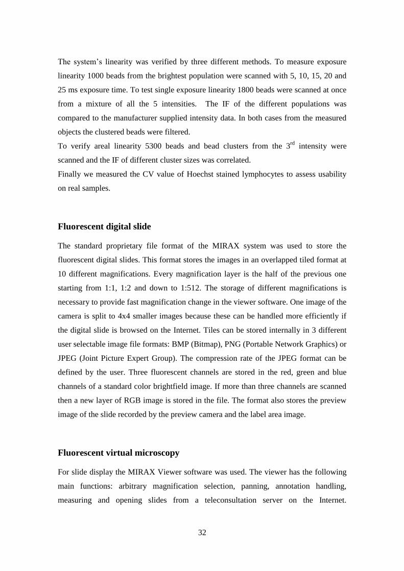
Without shading compensation, CV of the specimen was 24.3% (Figure 8A). After the
use of the white and black reference images for compensation without image
compression, the CV decreased to 3.9% (Figure 8B).
36
Figure 8. CV of the integrated fluorescence values of standardization beads with and
without compensation. The dark gray columns represent the measured single beads and
the light gray columns the doublets, clusters and other artifacts that were gated out based on
area and perimeter. A: IF histogram of single gated beads without compensation, 535 beads
are measured. CV: 24.3%. B: IF histogram of the same beads with compensation, 529
beads are measured. Some beads fell out of the original gate after compensation. CV: 3.9%.
C: On the left, 6 beads without compensation and on the right the same beads after
compensation. The beads are in focus, the difference in intensity is only because of the
uneven illumination. D: The white compensating image used for shading compensation in
this example. In case of ideal illumination the whole image should be uniform and bright.
In reality, the upper left part is 2.6 times brighter than the lower right. The bit depth of the
image is 8-bit; the brightest area’s gray level value is 205 and the dimmest gray level value
is 78.
For testing the system’s linearity, two methods were applied. The first method is to scan
a homogenous fluorescence bead sample multiple times using different exposure times
and calculate the correlation of the integrated fluorescence’s mean value. With exposure
times between 1,000 and 4,000 msec in 500 msec steps, the integrated fluorescence and
exposure times’ correlation was 0.999963 (p < 0.0001).
The second method is to compare the fluorescence ratio of different beads measured on
FCM and SFM. The beads were measured on a FACScan (Becton, Dickinson and Co.,
Franklin Lakes, NJ) (Figure 9A). The ratio of the two brightest peaks on FCM was 4.11

37
and on SFM 4.00. The ratio of the second and third peak was 3.84 on FCM and 10.67
on SFM (Figure 9A,B). Manufacturer specified all ratios to be 4.0.
Figure 9. Linearity of the integrated fluorescence measurement. A: Fluorescence
histogram of four different bead intensities measured on Flow. R3’s mean = 60.3, R4’s
mean = 231.5 and R5’s mean = 952.6. Ratio of R5 mean and R4 mean is 4.11, and ratio of
R4 mean and R3 mean is 3.84. Doublets were gated out. B: IF histogram of the same beads
measured with SFM. R3’s mean = 624, R4’s mean = 6,649, R5’s mean = 26,605. The ratio
of R5 and R4 is 4.001 and ratio of the R4 and R3 is 10.67. Manufacturer specified all ratios
to be 4.0. The dark gray columns represent the measured single beads and the light gray
columns the doublets, clusters and other artifacts that were gated out based on area and
perimeter.
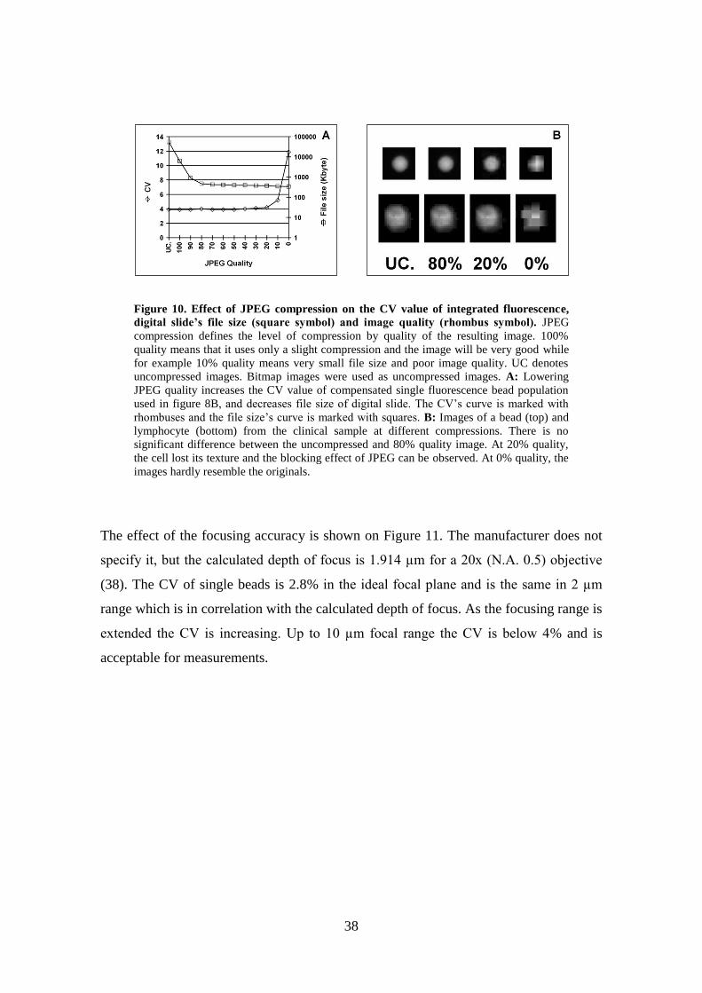
The effect of image compression can be evaluated by the results in Figure 10.
It was found that using standard JPEG, up to a compression ratio of 1:150, the CV does
not change significantly (Figure 10A). A general property of lossy image compression
technologies, such as JPEG, is that the loss is in the resolution domain and not in
intensity. Since the quality measurement is based on integrated fluorescence or
intensity, the CV is good at high compression rates but the image quality is not
acceptable (Figure 10B). The best compromise in compression is between 1:50 and
1:100, in this range the CV and image quality is still very good but the size is reduced
dramatically. Standard JPEG defines the compression in image quality instead of ratio;
the compression quality between 90% (1:61) and 80% (1:116) provided images suitable
for future use. The quality percentage does not relate to exact compression ratios; other
samples would have different ratios for the same quality settings. The newer version of
JPEG, JPEG 2000 uses compression ratios directly thus the final file size can be better
controlled. JPEG 2000 uses new image compression techniques too, and will probably
provide better quality at the same compression rate (37).
38
Figure 10. Effect of JPEG compression on the CV value of integrated fluorescence,
digital slide’s file size (square symbol) and image quality (rhombus symbol). JPEG
compression defines the level of compression by quality of the resulting image. 100%
quality means that it uses only a slight compression and the image will be very good while
for example 10% quality means very small file size and poor image quality. UC denotes
uncompressed images. Bitmap images were used as uncompressed images. A: Lowering
JPEG quality increases the CV value of compensated single fluorescence bead population
used in figure 8B, and decreases file size of digital slide. The CV’s curve is marked with
rhombuses and the file size’s curve is marked with squares. B: Images of a bead (top) and
lymphocyte (bottom) from the clinical sample at different compressions. There is no
significant difference between the uncompressed and 80% quality image. At 20% quality,
the cell lost its texture and the blocking effect of JPEG can be observed. At 0% quality, the
images hardly resemble the originals.
The effect of the focusing accuracy is shown on Figure 11. The manufacturer does not
specify it, but the calculated depth of focus is 1.914 µm for a 20x (N.A. 0.5) objective
(38). The CV of single beads is 2.8% in the ideal focal plane and is the same in 2 µm
range which is in correlation with the calculated depth of focus. As the focusing range is
extended the CV is increasing. Up to 10 µm focal range the CV is below 4% and is
acceptable for measurements.

39
Figure 11. Effect of focusing accuracy on the CV value of the integrated fluorescence
(IF) of the standardization beads. One field of view of beads was recorded in 1 µm steps
from –10 µm to +10 µm from the ideal focal plane. From the single images, several digital
slides were made corresponding to a certain focus range. On these created slides, the CV of
the populations was measured. There were 48 single beads and 3 clusters in the field of
view. In our measurements the focus range is always an even number because it includes
the same number of focal planes in plus and minus directions. In this case, we defined the
focus range of 10 µm (±5 µm) acceptable because the CV of single beads remained below
4%.
The system was also tested with a slide of Hoechst stained lymphocytes. The scatter
plot of area and perimeter, histogram of integrated fluorescence and a portion of the
cell’s gallery are presented in Figure 12. The CV of the gated population shown in
Figure 12A was 5.6%.

40
Figure 12. Application of the technique on a clinical specimen (Hoechst stained Ficoll
separated lymphocytes) and the use of the scatter plot and histogram linking. A:
Ungated scatter plot of the sample. Since SFM can not measure forward or side scatter, cell
area and perimeter values are used to gate debris and clumps. B: Histogram linked from the
gated scatter plot. The dark gray columns represent the cells inside the gate and the light
gray columns the cells outside the gate. C: Portion of cell’s gallery. Gallery is of cells
contained within the gate shown in scatter plot A; the cells are shading compensated.
Comparison of SFM, FCM and LSC
In this study the goal was to use for comparison the same sample for all three
techniques. Therefore two different DNA dyes and ECD labeling was used (with broad
excitation (460-600nm) and emission (555-680 nm) spectrum) to overcome the problem
of different excitation and emission spectra of the detection modalities of each
instrument (SFM, LSC, FCM). The FITC and ECD labeling was detectable by all three
instruments (Figure 13). For nuclear counter staining TOTO-3 and Hoechst 33258 were
detectable by the LSC (CV range 12-14%) and the SFM (CV range 6-8%), respectively.
The relatively high CV value in TOTO-3 staining did not impede finding cells by the
LSC. In our experiments we did not use permeabilisation and RNA-se treatment, so

41
DNA staining could be heterogeneous and TOTO-3 could bind to RNA also (39) giving
broad variance in TOTO-3 fluorescence.
High concentration samples for relative cell frequency determination by
FCM and SBC measurements
In the measurements the most suitable fluorescence detection of cell surface markers
were shown by the FCM followed by SFM and LSC. In the FCM measurements on the
dot plots there are clearly distinguishable cell populations (Figure 13C), which are less
distinct with SFM and LSC (Figure 13A,B). If the gating is not correct (for FCM), due
to the lack of visual reinspection, several events can be classified as false positives.
Figure 13. Differentiation of peripheral blood cells and HT29 tumor cells by the three
modalities. Scatter plots show clearly distinguishable peripheral blood cell (R2) and HT29
population (R3). by SFM (A), LSC (B), and FCM (C). X axis CAM5.2 FITC labeling, Y
axis CD45 ECD labeling. With SFM and LSC a relatively high aspecific red fluorescence
of the CAM5.2 FITC labeled tumor cells was detected. Therefore the HT29 cell population
shows unexpectedly high ECD values. This fluorescence was compensated in the LSC and
FCM measurements.
R2 R3
R2 R3
R2
R3

42
However, the correlation between the measured and expected cell frequency (Figure
14.) was the highest (r2 = 0.84; p<0.01) with FCM, followed by the SFM (r
2 = 0.79;
p<0.01) and LSC (r2 = 0.62; p<0.01). In the FCM measurements one of the three
replicates series showed outlier results. If we exclude these data from the evaluation
even higher reproducibility can be achieved (Figure 14C). LSC showed systematically
higher relative tumor cell frequencies as the calculated value. SFM showed the highest
variation in the measured cell frequencies. The measurement time for the evaluation of
the sample by the flow cytometer took 3-5 min, on the LSC 10-15 min, on the SFM 40-
50 min.
Figure 14. Correlation of determined and expected cell frequencies. Regression lines
showing correlation between the expected (diluted, Y) and determined (X) cell frequencies
of HT29 cells to peripheral blood cells in dilution series (1:1 to 1:1000) by SFM (A), LSC
(B) and FCM (C), respectively. At each concentration at least three samples were prepared
and measured.
FCM Measurements
HT29_WBC Dilution
0,001 0,01 0,1 1
FCM Ratio
0,001
0,01
0,1
1
LSC Measurements
HT29_WBC Dilution
0,001 0,01 0,1 1
LSC Ratio
0,001
0,01
0,1
1
SFM Measurements
HT29_WBC Dilution
0,001 0,01 0,1 1
SFM Ratio
0,001
0,01
0,1
1
A B
C
43
Low concentration samples for absolute cell frequency determinations
(SBC measurements)
If we placed by micromanipulator 5, 10, 20 or even 50 fluorescent labeled cells into the
measuring tube (5 mL tube, 100 L cell solution) we could not detect any FITC labeled
cell by FCM. In the case of the circulating tumor cells we could not compare the same
preparation because of lost cells after FCM. Therefore in the low concentration
specimen we could compare only SFM and LSC with visual reevaluation of the same
slides.
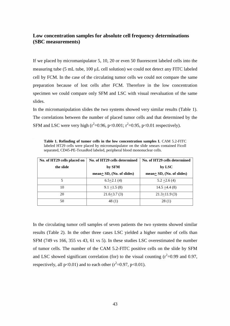
In the micromanipulation slides the two systems showed very similar results (Table 1).
The correlations between the number of placed tumor cells and that determined by the
SFM and LSC were very high (r2=0.96, p<0.001; r
2=0.95, p<0.01 respectively).
Table 1. Refinding of tumor cells in the low concentration samples I. CAM 5.2-FITC
labeled HT29 cells were placed by micromanipulator on the slide smears contained Ficoll
separated, CD45-PE-TexasRed labeled, peripheral blood mononuclear cells.
No. of HT29 cells placed on
the slide
No. of HT29 cells determined
by SFM
mean+ SD, (No. of slides)
No. of HT29 cells determined
by LSC
mean+ SD, (No. of slides)
5 6.5+2.1 (4) 5.2 +2.6 (4)
10 9.1 +1.5 (8) 14.5 +4.4 (8)
20 21.6+3.7 (3) 21.3+11.9 (3)
50 48 (1) 28 (1)
In the circulating tumor cell samples of seven patients the two systems showed similar
results (Table 2). In the other three cases LSC yielded a higher number of cells than
SFM (749 vs 166, 355 vs 43, 61 vs 5). In these studies LSC overestimated the number
of tumor cells. The number of the CAM 5.2-FITC positive cells on the slide by SFM
and LSC showed significant correlation (for) to the visual counting (r2=0.99 and 0.97,
respectively, all p<0.01) and to each other (r2=0.97, p<0.01).

44
Table 2. Finding of tumor cells in the low concentration samples II. Absolute numbers
of magnetic isolated circulating tumor cells as detected by SFM, LSC and microscopy in
colorectal cancer patients.
Patient ID No. of CAM5.2+ cells
SFM
No. of CAM5.2+ cells
LSC
No. of CAM5.2+ cells
Visual observation
1 2 1 0
2 5 61 2
3 80 59 78
4 14 0 15
5 166 749 164
6 0 0 0
7 43 355 39
8 0 11 0
9 4 1 6
10 13 4 9
Quantitative and stoichiometric fluorescent whole slide imaging
Focusing
The objective has a calculated 0.57 µm depth of field at the 605 nm emission
wavelength of the Rhodamine filter (38). One step of the focus motor is 0.2 µm that is
almost 3 times smaller as the depth of field thus the fine focus algorithm steps always in
2 motor steps (0.4 µm) because this is sufficient. Table 3 sums the differences between
the automatically found and the manually fine tuned focus levels.
Ninety-three percent of the field of views did not differ at all or the difference was less
than the depth of field. Within the depth of field some visual differences are observable
but this does not influence the information content of the image. The observer might
pick another field of view as an algorithm.

45
In 7 percent of the cases the difference was 0.8 µm. It means only one step error since
the smallest step the algorithm is making is 0.4 µm. Subjectively assessed these images
are still well focused.
Table 3. Focus level differences. The left column shows the difference in µm between the
automatically found focus levels and the manually fine focused position. The right column
shows how many field of views were found with the given difference.
Difference in µm Number of field
of views
-0.8µm 3
-0.4µm 17
0 µm 54
+0.4µm 22
+0.8 µm 4
Scanning results
The marker pen based sample detection worked reliably if the marking was at least 1
mm wide and fully connected in the area imaged by the preview camera. The preview
camera grabs 30 frame per second thus preview image capture time is negligible in the
whole process.
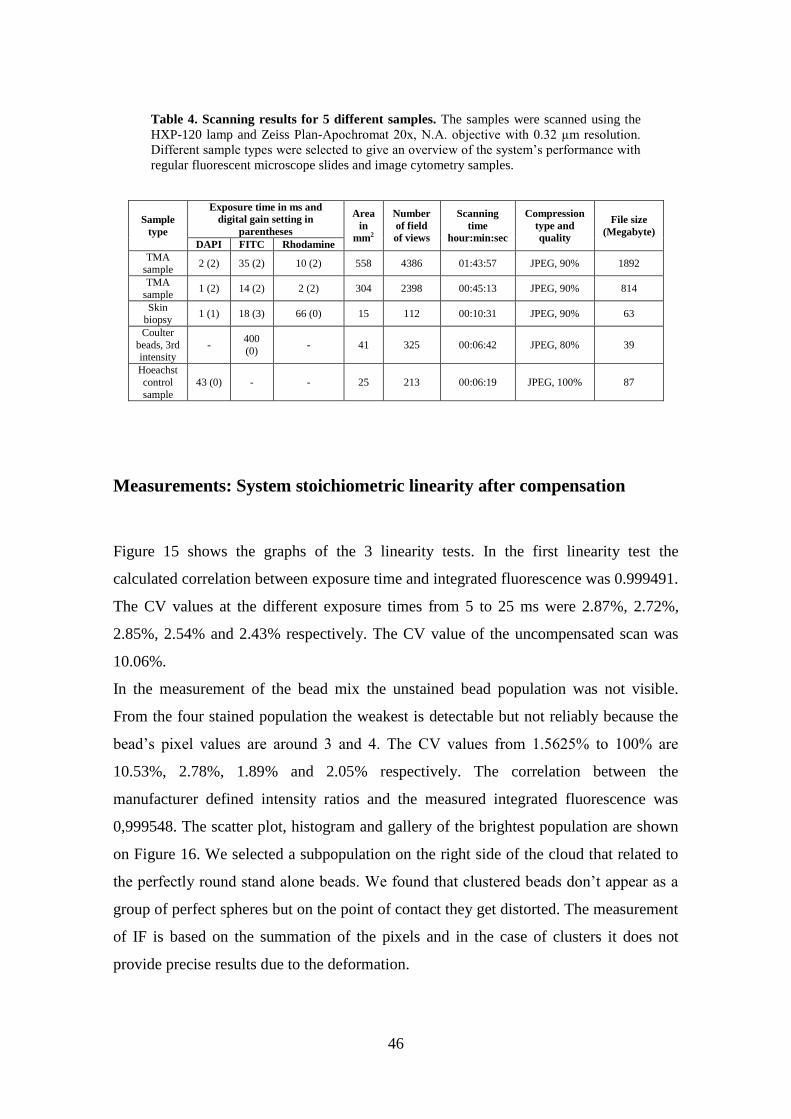
Exposure times and focusing speed is proportional the staining intensity. Table 4
summarizes the scanning information for 5 different samples.
46
Table 4. Scanning results for 5 different samples. The samples were scanned using the
HXP-120 lamp and Zeiss Plan-Apochromat 20x, N.A. objective with 0.32 µm resolution.
Different sample types were selected to give an overview of the system’s performance with
regular fluorescent microscope slides and image cytometry samples.
Sample
type
Exposure time in ms and
digital gain setting in
parentheses
Area
in
mm2
Number
of field
of views
Scanning
time hour:min:sec
Compression
type and
quality
File size
(Megabyte)
DAPI FITC Rhodamine
TMA sample
2 (2) 35 (2) 10 (2) 558 4386 01:43:57 JPEG, 90% 1892
TMA
sample 1 (2) 14 (2) 2 (2) 304 2398 00:45:13 JPEG, 90% 814
Skin biopsy
1 (1) 18 (3) 66 (0) 15 112 00:10:31 JPEG, 90% 63
Coulter
beads, 3rd intensity
- 400
(0) - 41 325 00:06:42 JPEG, 80% 39
Hoeachst
control
sample
43 (0) - - 25 213 00:06:19 JPEG, 100% 87
Measurements: System stoichiometric linearity after compensation
Figure 15 shows the graphs of the 3 linearity tests. In the first linearity test the
calculated correlation between exposure time and integrated fluorescence was 0.999491.
The CV values at the different exposure times from 5 to 25 ms were 2.87%, 2.72%,
2.85%, 2.54% and 2.43% respectively. The CV value of the uncompensated scan was
10.06%.
In the measurement of the bead mix the unstained bead population was not visible.
From the four stained population the weakest is detectable but not reliably because the
bead’s pixel values are around 3 and 4. The CV values from 1.5625% to 100% are
10.53%, 2.78%, 1.89% and 2.05% respectively. The correlation between the
manufacturer defined intensity ratios and the measured integrated fluorescence was
0,999548. The scatter plot, histogram and gallery of the brightest population are shown
on Figure 16. We selected a subpopulation on the right side of the cloud that related to
the perfectly round stand alone beads. We found that clustered beads don’t appear as a
group of perfect spheres but on the point of contact they get distorted. The measurement
of IF is based on the summation of the pixels and in the case of clusters it does not
provide precise results due to the deformation.
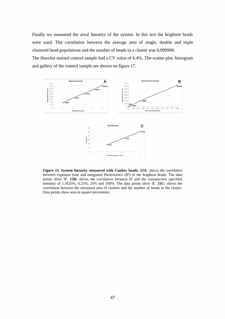
47
Finally we measured the areal linearity of the system. In this test the brightest beads
were used. The correlation between the average area of single, double and triple
clustered bead populations and the number of beads in a cluster was 0,999998.
The Hoechst stained control sample had a CV value of 6.4%. The scatter plot, histogram
and gallery of the control sample are shown on figure 17.
Figure 15. System linearity measured with Coulter beads. 15A: shows the correlation
between exposure time and integrated fluorescence (IF) of the brightest beads. The data
points show IF. 15B: shows the correlation between IF and the manufacture specified
intensity of 1.5625%, 6.25%, 25% and 100%. The data points show IF. 15C: shows the
correlation between the measured area of clusters and the number of beads in the cluster.
Data points show area in square micrometer.
A B
C

48
Figure 16. Scatter plot, histogram and gallery of a bead population. Beads on a slide
with 5 different intensities are scanned. 16A: Shows the scatter plot of the brightest beads.
Shape Factor is displayed versus Area. Clustered beads are deformed and to measure
intensity precisely the stand alone perfectly round objects are selected as a sub population
on the right of the cloud. 16B: Shows the histogram derived from the scatter plot. The
green marker lines delimit the final measured data set. 16C: Shows a portion of the bead
gallery derived from the histogram.
CC
AA BB

49
Figure 17. Scatter plot, histogram and gallery of the Hoechst stained control sample.
The population of lymphocytes were selected on the scatter plot based on area and
perimeter. Artifacts were rejected on the histogram based on integrated fluorescence and
215 cells were selected for CV measurement. The gallery shows some of the lymphocytes.
CC
AA BB

50
DISCUSSION
Scanning Fluorescent Microscopy
Fluorescent cell measurements are superior to transmitted light determinations due to
the higher sensitivity, absence of the distribution error, and a greater number of
simultaneously measurable molecular species. A major advantage of slide based
microscopic measurements is that they can be performed in parallel or sequentially.
The earlier automation of flow cytometry systems in sample handling and higher
measurement speed (6) are the cause of the overall dominance of FCM in cell analytics
over microscope based systems. However, the lack of opportunity for the morphological
relocation of selected cells proved to be one of the most limiting factors of this
technology.
The work of Kamentsky et al. (18) on the development of a laser scanning cytometry
system, the LSC aimed to fulfill these requirements. The broad range of applications
and papers with the LSC system shows, that this technology has real acceptance by
cytometrists (7, 9, 18, 19, 40-44).
Automated fluorescent microscopy attempts have shown the close correlation of the
measured fluorescence parameters to FCM (14,15).
However, the principle of on-line measurements of the multi-fluorescent labeled cells
and not storing the single field of views caused the loss of one of the most important
features that microscopy can yield: the correlation of the measured parameters to
morphological data.
This approach has several advantages over FCM and LSC. To add a new stain with new
excitation and emission wavelengths requires only a new filter block; while, using the
other two modalities requires the installation of a new laser and photomultiplier.
Making a digital slide from the original is ideal for archiving and documentation. The
digital slide can be sent through the Internet to fellow researchers or students can take it
home on a DVD. Because fluorescent samples fade, in some days or weeks, the sample
might become useless. Arbitrary selection of cells can be displayed in galleries in
seconds, because every cell’s image can be accessed in a random manner from the

51
digital storage. This feature gives real freedom for the morphological analysis, which is
missing in FCM.
For rare-cell detection, scanning the complete sample provides the safety of not losing
any cells. The off-line evaluation permits the measurements to be repeated using
different parameters as long rare cells are found. The digital slide also permits the
evaluation of fluorescent histological samples because the process is not limited to a
single field of view.
The main problem of quantitative measurement using mercury arc lamps is the none
uniform illumination. Scrambling the light with a fiber optic or liquid light guide (24)
was not available through standard commercial channels for all the microscope used in
this work.
In the LSC, the scanning laser beam provides a constant intensity in every part of the
field of view. Since this is not the case for arc illuminated microscopes, the illuminated
reference (white) image and CCD dark current noise reference (black) image were used
for compensation. The first one is called white because in the case of an ideal
illumination all of its pixels should be white but not saturated. The white image is for
correcting the error of the lamp; the black image corrects the error of the camera. The
pixels of a CCD camera’s picture are higher than zero even if there is no light at all.
This error means a constant positive shift in the pixel values. On the black reference
image, every pixel should be zero in the ideal case. The use of these two images with
equation 1., compensates the raw images so effectively that the system provides
comparable data to FCM or LSC.
In the compensation example in Figure 2B, mean of the uncompensated beads is 156.2,
standard deviation is 60.9 and CV is 39%. The mean of the compensated beads in
Figure 2C is 231, standard deviation is 0 and CV is 0%. Compensation scales up gray
level values to the brightest level, thus the new mean is always higher than the original.
The same effect can be observed in Figure 8A and 8B, in the uncompensated histogram
just few beads are above 30,000 and in the compensated one, all of them are around this
value. In the example, beads are brighter than the white reference image. This is not a
contradiction; white reference does not have to be the brightest value; it has to represent
the illumination pattern. We chose up-scaling over downscaling, because downscaling
would lose information.

52
SFM stores the original image for every field of view in every channel, plus one
common black reference image and one white reference image for every channel.
Compensation is done always on the fly during slide viewing or image processing.
Compensation is applied to every fluorescent channel of a field of view and of course
must be repeated for every field of view. This approach yields slower viewing and
image processing compared to stored compensated images but the goal was to maintain
maximum confidence and verifiability. It can be always checked in the digital slide
viewer how did the original image look like, was it saturated or did the compensation
introduce any artifacts.
The results show, that using compensation slides, image compression techniques,
sophisticated autofocusing strategy with the implementation of standard cytometry
techniques an applicable working environment was developed.
Model et al. found that concentrated fluorophores between standard slides and coverslip
are better for shading correction than commercial fluorescent slides or fluorophores in
chamber (45). They used a similar method as ours for shading correction but did not
measure large cell or bead populations. Lockett et al. used beads for shading
compensation (17). Their results are better but they did not measure large cell or bead
populations either. Instead of grabbing a single field of view of fluorophores they
position one bead or cell to multiple locations in the field of view. They calculate a
compensation image based on the intensity of the same object in the different locations.
The consequence of this method is that they also have to compensate for the photo
bleaching of the object.
Concerning the linearity of the system, in the second ratio of the fluorescence of the
standardization beads, the great difference between FCM and SFM is due to the
dynamic range. The flow cytometer used for this study in FCM had a 10 bit range and
in the SFM system the camera’s bit depth was set to 8 bits. The ratio of the first peak
and the third peak according to the FCM measurement was around 16. On the 8 bit
image the brightest pixels of a bead had a value of 240. 240 divided by 16 results in 15.
If the brightest pixel of the spherical bead is 15 then the edge of the bead fades into the
background and is cut off by the threshold and the integrated fluorescence is calculated
on a smaller area. The fluorescence dynamic range is around 1:6 using 8 bit depth. FCM
and SFM dynamic range can not be compared directly because in real life the integrated

53
fluorescence value also depends on the size of the cells. Due to its measurement method
SFM’s dynamic range is comparable to FCM because it can measure objects up to the
size of a field of view. AxioCam has 14 bit depth and other commercially available
Peltier cooled, monochrome cameras have also 12 bit ADCs and often less than 5
photoelectrons residual noise. In this study, we used the lower 8 bit of AxioCam’s 14 bit
depth to decrease acquisition time. Fluorescence values are different in Figures 9A and
9B because both systems use arbitrary units for quantification. In this measurement the
flow cytometer had a 10 bit analogue to digital converter, thus the highest measurable
value is 1023. In the SFM measurement, one bead’s image had approximately 200
pixels. 200 multiplied by 255, the maximal gray level of an 8 bit image, results in
51,000 which is the highest theoretical integrated fluorescence value for a bead with this
bit depth and magnification.
SFM stores every channel in every field of view; therefore the final file sizes would be
very large without image compression. Using standard JPEG lossy image compression,
acceptable file sizes and image quality were achieved. Standard JPEG supports only 8
bit depth, but the digital camera used provided 14 bit images. Since we had to sacrifice
6 bits anyway we chose the lowest 8 bit of the camera to have as short exposure times
as possible to increase scanning speed.
Our technology still uses a commercially available, motorized fluorescent microscope.
The advantage of this technique is that these microscopes can be used as a manual tool
for standard microscopy. Also, with our technique, they can be converted into a multi-
channel fluorescent scanner. This technique could be enhanced by sophisticated
biotechnology methods for the evaluation of large number of antigens (46).
The disadvantages of our system are also clear: manual slide loading and scanning area
definition are still necessary, which costs time and manpower. Some companies have
developed slide loaders for example in the field of cervical cytology analysis. These
loaders are only available as a part of a complete and closed system and currently they
are not open to apply other applications like SFM.
The development of Bajaj et al. (1) decreases the autofocusing time at least by an order
of magnitude. However, their work was done also around a commercial inverted
microscope. A new attempt for automation and enhanced detection was described by
Tibbe et al. (47) using magnetic cell isolation and compact disc technology.

54
With the enhanced focus on the medical interest in circulating tumor cells and other rare
cells (stem cells, malignant residual disease, organ specific stem cells in histological
sections) the mainstream of cell analytical research will need novel microscopy based
techniques.
Comparison of SFM, FCM and LSC
Detection of circulating tumor cells is of substantial clinical importance and its
prognostic value has been demonstrated (48). Our results on the 10 patient sample show
that SFM has a good potential for finding the fluorescent labeled tumor cells
contributing to the analysis and solution of this clinical problem and is equivalent to
LSC and FCM. For further validation of the SFN method, a significantly higher number
of patient samples are required of course. Alternative, highly sensitive assays like RT-
PCR were found to show false positive results in tumor free patients (49). Cytokeratin,
as marker of the epithelial cancer cells is also expressed in gastrointestinal
inflammations in lymphocytes (50). Therefore RT-PCR or immunohistochemistry alone
is not sufficient for reliable micrometastases detection. Today FDA approved automated
microscopy systems exist only for enzyme based micrometastases detection
(Chromavision Inc., Applied Imaging Inc.).
However, more and more information appears, that fluorescent cell detection with
multiple labeling would have greater specificity and sensitivity (32).
As fluorescent microscopy is becoming more and more widespread and is used in
clinical and basic research automation is of increasing necessity. Until now the
automation was done using the traditional epifluorescent (32) or inverted microscopy
stages (1, 29), which were designed for manual use, not for high throughput.
One of the most problematic issues in automation is autofocusing. Image analysis based
autofocusing is time consuming. This is in agreement with our own experience.
Automated slide loading also has not been solved in these applications. As requirements
from the users become obvious for automation, and algorithms are available for
automated scanning and evaluations, results with new automated and fast scanning
hardware systems are expected (51). The acquisition speed for SFM is slower than that
of the LSC, while FCM is the fastest technology.

55
Comparative studies with FCM and LSC have shown that data obtained by both
technologies are consistent with each other to study apoptosis or necrosis (52). LSC is a
reliable tool for the intracellular staining of p53 protein (41) and DNA ploidy analysis
(42). Moreover SBC (LSC) provides a number of benefits that may make it more
suitable for clinical laboratories than FCM (43). Even serial immunostaining could be
performed for an increased number of fluorescence parameters (46).
In a comparison between LSC, FCM and image cytometry linear regression analysis of
DNA ploidy data and SPF values of tumors also showed statistically significant
agreement (44).
This comparison of three methods showed that the fluorescent measurements on cell
suspension or smears in dilution series yield similar results for the tumor cell /
lymphocyte ratio both in the high and low concentration ranges. Similar studies were
performed with similar results using LSC and FCM (41), and image analysis and FCM
(53).
In the range of the very low frequency of the tumor cells FCM has some disadvantages
finding the 1-2 cells per sample. Similarly, the determination of the tumor cell
concentration in the peripheral blood by FCM is unsatisfactory if the sample contains
only one or two tumor cells.
FCM is a so called population measurement, because data from many thousand cells are
acquired, on a dot plot similar signals give a group belonging together, but one or two
cells do not. Cell aggregates could give signals out of scale and are therefore lost from
analysis. The measured objects are unavailable for visual morphological inspection and
are lost after the acquisition. Since the cell can not be relocated, we have to believe the
data. Confirmation of the morphology could be done by sophisticated cell sorting or
new in flow imaging technology (54-57).
After isolation of the cells from the blood the whole sample volume should be
measured. A problem arises while measuring the last drops of the cell suspension
(looking for all tumor cells from the patient sample), because air bubbles in the flow
channel may cause strong light scattering and many false signals are acquired resulting
in an analysis that is at least partially based on this artifact. Time gating of the data until
the first air bubble could help the analysis.

56
SFM software using a commercial microscope and camera provides similar quality of
finding fluorescence labeled rare cells as the LSC. SBC proved to be more suitable for
the rare cell detection than FCM. Due to the interactive threshold determination,
standard cytometry techniques and human reevaluation of the digital slides SFM may
prove an acceptable adaptation of conventional fluorescent microscopes in order to
perform rare cell detection.
Quantitative and stoichiometric fluorescent whole slide imaging
Sample detection and localization
MIRAX MIDI is an automated whole slide imager with a slide loading capability for 12
slides. To enable automated fluorescent scanning it is important to develop an
automated specimen detecting and locating method. Fluorescent samples have low
contrast in normal brightfield imaging and they can not be detected by the preview
camera. The possible alternative solutions could be low magnification fluorescent,
darkfield or phase contrast imaging or manual sample marking. The first three methods
would require an objective changer to use a low magnification objective to generate a
slide preview. In fluorescent imaging the intensity is calculated by the following
equation:
𝐼𝑛𝑡𝑒𝑛𝑠𝑖𝑡𝑦 ≈𝑁𝑢𝑚𝑒𝑟𝑖𝑐𝑎𝑙 𝐴𝑝𝑒𝑟𝑡𝑢𝑟𝑒4
𝑀𝑎𝑔𝑛𝑖𝑓𝑖𝑐𝑎𝑡𝑖𝑜𝑛2
Low magnification objectives have low numerical apertures that result 1000 times
longer exposure times compared to the 20x objective used in this study which is
absolutely impracticable. Darkfield illumination and phase contrast would require a
different condenser design that could not be fitted in the MIRAX MIDI because of the
tight construction of the quick focusing mechanism. Due to the optical and mechanical
57
constraints the marker pen based method was used which requires negligible extra
burden from the users. The existing hardware could be used without any modifications,
and it worked well on all samples.
Automatic focusing
The required exposure time to image fluorescent stains by a microscope can vary from
few milliseconds to several thousands or in other words the system has to focus samples
with a dynamic range of 1:1000. The dynamic range of the AxioCam MRm is 12 bits
but it was used in 8 bit mode because the complete MIRAX software package has 8 bit
internal image handling.
The theoretical dynamic range of an 8 bit imaging device would be 1:255 but in practice
the electronic and photon shot noise decrease it (36). The electrical noise of the
AxioCam MRm was negligible in 8 bit mode. Photon shot noise equals to the square
root of the photons of a pixel. At low light intensities shot noise dominates the pixel
differences and not the actual sharpness thus dark images are not sufficient for focusing.
According to our tests if the brightest pixels were in the pixel value range of 32 and 64
then the calculated sharpness values were reliable for most samples. Low contrast
samples needed a range from 64 to 128 or from 128 to 255. We concluded that an 8 bit
camera has a practical dynamic range of 1:8 (32:256) if images appropriate for focusing
have to be grabbed. Our solution to find the right focus level of samples with a higher
dynamic range was to continuously change the exposure time during the focusing
process. A fixed long exposure time would saturate the sample and a short exposure
could miss faint samples.
The brightfield sharpness calculation algorithm of the MIRAX software worked well on
fluorescent tissue samples. However on cell samples especially if there were only few
cells in the field of view the algorithm did not work reliably. The brightfield focus
algorithm calculates and sums the value differences of neighboring pixels. A
lymphocyte has 7 µm diameter what is represented roughly by 370 pixels with 0.3225
58
µm / pixel resolution. 370 pixels are 0.026% of the active pixels of the camera and the
pixel differences of the cell disappear in the sum of differences of the background noise.
Our strategy was to enhance the higher differences with lower occurrence and suppress
small differences with high occurrence. The goal was to have a general algorithm so we
did not want to use a fixed threshold to separate the background from the samples.
Instead of simply summing the differences the algorithm generates a histogram. This
way the pixel value differences are grouped and can be differentiated. The columns
were summed after being multiplied by the column indices to the power of 5. This
exponential value was determined by experiments and worked reliably on all samples.
Figure 18 shows a field of view in two different focus positions and the corresponding
histogram curves.
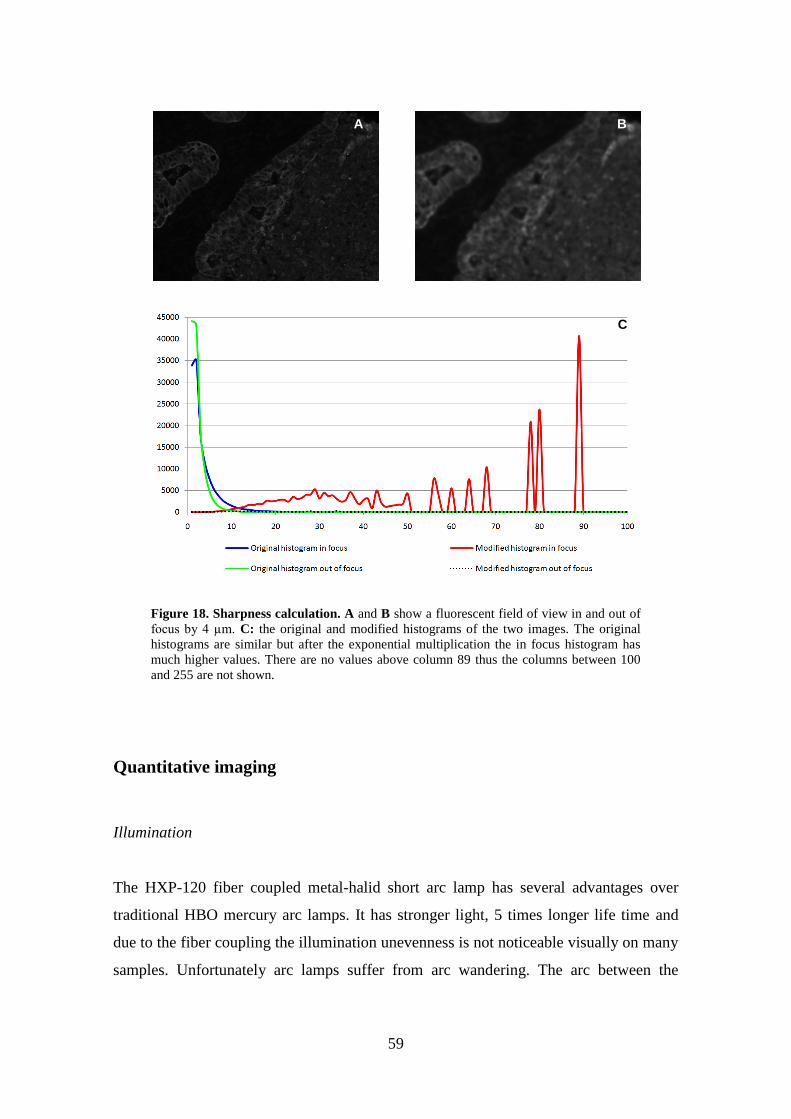
59
Figure 18. Sharpness calculation. A and B show a fluorescent field of view in and out of
focus by 4 µm. C: the original and modified histograms of the two images. The original
histograms are similar but after the exponential multiplication the in focus histogram has
much higher values. There are no values above column 89 thus the columns between 100
and 255 are not shown.
Quantitative imaging
Illumination
The HXP-120 fiber coupled metal-halid short arc lamp has several advantages over
traditional HBO mercury arc lamps. It has stronger light, 5 times longer life time and
due to the fiber coupling the illumination unevenness is not noticeable visually on many
samples. Unfortunately arc lamps suffer from arc wandering. The arc between the
A B
C
60
electrodes of the lamp jumps from time to time to another point on the electrodes and
change the illumination pattern and intensity (58). If the illumination pattern changes
the prerecorded compensation images are not sufficient anymore. We found that the
mechanical position of the fiber can also change the illumination pattern. These
properties make the metal-halid lamp impractical for quantitative measurements. The
Colibri lamp provided very stable illumination in time and it is mounted directly on the
microscope without a fiber. These features made this lamp the optimal choice for
quantitative analysis.
The power of the two light sources is not directly comparable because their spectral
characteristics are different but our experience was that the Colibri was 20-30% weaker
on average. The meta-halid lamp emits light from 300 nm to 700 nm with the same peak
wavelengths as HBO lamps (365, 405, 436, 546, 579 nm). The peaks are weaker
compared to HBO but between the peaks the light is stronger. LED modules for the
Colibri lamp are available at 365, 380, 400, 455, 470, 505, 530, 590, 615 and 625 nm
wavelengths.
Compensation slide
The manually prepared slides used in SFM could contain bubbles, dust particles and
other artifacts. The proper field of views had to be selected manually. The thin polymer
section used in this study covered the complete slide and we did not detected
irregularities. The described compensation image creation algorithm always provided
good results. The laser dyes in the compensation slide bleach. Our algorithm picks only
10 field of views randomly thus slides can be used several times. It is important to focus
the compensation slide to map as good as possible the illumination pattern. The FITC
solution was easy to focus because of the mentioned artifacts. On the polymer slide the
focus could not be determent based on the sample structure. The slide was focused by
selecting the motor position which provided the brightest image based on the properties
of exposure and focus shown on Figure 5.
Image segmentation and measurement

61
Manually set threshold values are necessary for segmentation because biological
samples are complex and an automated threshold algorithm cannot determine the goal
of a study. For example nucleus, cytoplasm, different cell populations and FISH spots
require different threshold values. The possibility to set different threshold values
within one measurement for the different targets is also necessary. In the linearity
measurement of beads with different intensities the following lower and upper threshold
values were used for the four populations: 4/7, 6/17, 15/70 and 60/255. If all four
populations would have been thresholded with a single pixel intensity level of 4 then the
bright beads would have approximately 2.7 times larger area because the background
around a bright object is also brighter. Upper thresholds are also practical to better
discriminate the different groups. In the other measurements one threshold value was
sufficient because in the case of areal linearity, different exposure times and
lymphocytes the populations had homogenous fluorescence intensity.
Advancements over SFM
The MIRAX MIDI hardware has several advantages over the regular AxioPlan 2
microscope. Its automated slide loader and preview camera makes it possible to digitize
several slides without manual interaction making the laboratory workflow more
effective.
The AxioCam HRc camera used in the SFM system is a color camera equipped with
piezo CCD sensor shift technology. This camera could record 13 megapixel in three
colors. The AxioCam MRm is a monochrome camera and can record only 1.3
megapixel images. The monochrome camera was chosen for the MIRAX system
because it had 2 times shorter exposure times what doubles the scanning speed. CCD
cameras are monochrome by nature and a color filter is placed in front of their pixels to
discriminate different wavelengths. While the characteristics of these filters usually
don’t match the fluorescent filter spectrum they absorb half of the light on average. The
pixel shift technology is slow and in a fast scanner its advantages can not be utilized.
The AxioCam MRm has also lower cost.

62
MIRAX MIDI has a 20x objective like the SFM system but with a higher N.A. and thus
it needs 6.55 times shorter exposure times for the same sample. In the SFM system the
lower 8 bits of the camera was used. Due to the higher light collecting capability in the
MIRAX system the upper 8 bit of the camera could be used which had lower noise. In
the SFM system only one threshold value was used for the objects. With the lower noise
and every populations individual threshold value all four bead populations could be
detected with appropriate intensity ratios while SFM could detect only 3 populations
and the intensity of the third population was measured 2.5 times lower as reality.
A new general focus algorithm had to be developed for the MIRAX system because the
algorithm used in SFM was not appropriate for tissue samples.
The new stable LED light source and compensation slide made it possible to achieve a
CV value of 1.9% while in the SFM system the best measured value was 2.8% on a
single field of view and 3.9% on a larger sample.

63
CONCLUSION
A motorized fluorescent microscope with the use of compensation slides and special
image processing algorithms can be used for quantitative and stoichiometric cytometry
measurements. Such a system provides comparable results with similar sensitivity and
specificity to well established Flow cytometry and Laser Scanning Cytometry. Slide
based image cytometry is superior to Flow Cytometry for rare cell detection.
With further development of the methods a fluorescent whole slide imager can be used
for quantitative and stoichiometric cytometry measurements. The technical
advancements of whole slide imaging over regular microscopy makes the clinical
workflow more effective in terms of reliability, speed, manpower and costs. With these
methods the clinical screening of colorectal cancer patients becomes possible.
64
SUMMARY
Recently enhanced focus is set on the rare cells of the human organ (circulating tumor
cells, physiologic and pathologic stem cells, fetal cells). Circulating tumor cells can be
detected in peripheral blood samples by cytometry. Slide based image cytometers
provide similar data as flow cytometry by digitally processing the cell images. For the
detection of circulating tumor cells, they have several advantages over FCM. In the
recent years brightfield whole slide imaging became commercially available and starts
to be established in pathology.
We created an imaging cytometer system called Scanning Fluorescent Microscope
(SFM) by using a motorized fluorescent microscope, special scanning and image
processing algorithms and a fluorescently stained compensation slide. We showed that
this system is capable of quantitative and stoichiometric measurements and it provides
comparable results to other well established cytometry solutions on large cell
populations. We showed that SFM detects rare cells more reliably as flow or laser
scanning cytometry.
We extended the commercially available MIRAX MIDI whole slide imager with
fluorescent scanning capability and used it with the SFM methodology. We showed that
the fluorescent whole slide imaging is possible and using the SFM methodology, it
provides even better results as the SFM system due to the technical advancements in
illumination and camera technology.
The automated slide loading, sample detection and scanning capabilities of whole slide
imaging systems combined with image cytometer software make possible the clinical
screening for colorectal cancer patients.
65
ÖSSZEFOGLALÓ
Az utóbbi időkben az emberi szervezet ritka sejtjeire fokozott figyelem irányul (keringő
daganat sejtek, fiziológiás és patológiás őssejtek, magzati sejtek). A keringő
daganatsejtek citometria segítségével mutathatók ki perifériás vérmintákban. A
tárgylemez képalkotó citométerek hasonló mérési adatokat szolgáltatnak, mint az
áramlási citométerek a sejtek képeinek digitális feldolgozásával. A keringő
daganatsejtek kimutatásában több előnyük is van az áramlási citometriával szemben. Az
utóbbi években az átmenőfényes teljes tárgylemez képalkotó (Whole Slide Imaging)
eszközök megvásárolhatóak lettek és kezdenek egyre szélesebb körben elterjedni a
patológiában.
Fluoreszcens motorizált mikroszkóp, speciális szkennelő és képfeldolgozó algoritmusok
és fluoreszcensen festett kompenzáló tárgylemez felhasználásával létrehoztunk egy
képalkotó citométer rendszert, amelyet Pásztázó Fluoreszcens Mikroszkópnak
(Scanning Fluorescent Microscope, SFM) neveztünk el. Megmutattuk, hogy ez a
rendszer képes kvantitatív és sztöchiometrikus mérésekre és más jól ismert citometriai
eljárásokkal összehasonlítható eredményt szolgáltat nagy sejtpopulációkon.
Megmutattuk, hogy az SFM rendszer ritka sejteket megbízhatóbban mutat ki, mint az
áramlási vagy a lézerpásztázó citometria.
A kereskedelmi forgalomban kapható MIRAX MIDI teljes tárgylemez képalkotó
rendszert kibővítettük fluoreszcens szkennelő funkcióval és az SFM metodikával
használtuk. Megmutattuk, hogy a fluoreszcens teljes tárgylemez képalkotás lehetséges
és az SFM metodika használatával még jobb eredményeket biztosít, mint az SFM
rendszer a megvilágítás és a kamera technika fejlődésének köszönhetően.
A teljes tárgylemez képalkotás automatikus tárgylemez adagoló, minta megtaláló és
szkennelő képességei, képalkotó citometriai szoftverrel együtt használva lehetővé teszik
a vastagbél-daganatos betegek klinikai szűrését.

66
LITERATURE CITED
1. Bajaj S, Welsh JB, Leif RC, Price JH. Ultra-Rare-Event Detection Performance
of a Custom Scanning Cytometer on a Model Preparation of Fetal nRBCs.
Cytometry 2000;39:285-294.
2. Borgen E, Naume B, Nesland JM, Nowels KW, Pavlak N, Ravkin I, Goldbard S.
Use of automated microscopy for the detection of disseminated tumor cells in
bone marrow samples. Cytometry (Communications in Clinical Cytometry)
2001;46:215-221.
3. Molnar B, Ladanyi A, Tanko L, Sreter L, Tulassay Z. Circulating tumor cell
clusters in the peripheral blood of colorectal cancer patients. Clin. Cancer Res.
2001;7:4080-4085.
4. Shapiro HM. Practical flow cytometry. 4th edition. Hoboken, NJ: Wiley-Liss;
2003. 681 p.
5. Shapiro HM. The evolution of cytometers. Cytometry Part A 2004;58:13–20.
6. Kukuck FW, Edwards BS, Sklar LA. High throughput flow cytometry.
Cytometry 2001;44:83-90.
7. Darzynkiewicz Z, Bedner E, Li X, Gorzycza W, Melamed MR. Laser-Scanning
Cytometry: A new instrumentation with many applications. Exp Cell Res
1999;249:1–12.
8. Tsavellas G, Huang A, Patel H, McCullogh T, Kim-Schulze S, Mersh TG: Flow
cytometric detection of circulating colorectal cells: works in vitro but not in
vivo. Eur. J. Surg. Oncol. 2001;27:778-779.
67
9. Gerstner A, Laffers W, Bootz F, Tarnok A. Immunophenotyping of peripheral
blood leukocytes by laser scanning cytometry. J. Immunol. Methods.
2000;246:175-185.
10. Ecker RC, Steiner GE. Microscopy-based multicolor tissue cytometry at the
Single cell Level. Cytometry Part A 2004;59:182-190.
11. Ecker RC, Rogojanu R, Streit M, Oesterreicher K, Steiner GE. An improved
method for discrimination of cell populations in tissue sections using
microscopy-based multicolor tissue cytometry. Cytometry Part A 2006;69:119–
123.
12. Szaniszlo P, Rose WA, Wang N, Reece LM, Tsulaia TV, Hanania EG, Elferink
CJ, Leary JF. Scanning cytometry with a LEAP: laser-enabled analysis and
processing of live cells in situ. Cytometry Part A 2006;69:641–651.
13. Jaggi B, Poon SS, MacAulay C, Palcic B. Imaging system for morphometric
assessment of absorption of fluorescence in situ stained cells. Cytometry
1988;9:566–572.
14. Galbraith W, Ryan KW, Gliksman N, Taylor DL, Waggoner AS. Multiple
spectral parameter imaging in quantitative fluorescence microscopy I:
quantitation of bead standards. Comput Med Imaging Graph 1989;13:47–60.
15. Galbraith W, Wagner MCE, Chao J, Abaza M, Ernst LA, Nederlof MA,
Hartsock RJ, Taylor DL, Waggoner AS. Imaging cytometry by multiparameter
fluorescence. Cytometry 1991;12:579–596.
16. Lockett SJ, O’Rand M, Rinehart CA, Kaufman DG, Herman B, Jacobson K.
Automated fluorescence image cytometry. DNA quantification and detection of
chlamydial infections. Anal Quant Cytol Histol 1991;13:27–44.

68
17. Lockett SJ, Jacobson K, Herman B. Quantitative precision of an automated,
fluorescence-based image cytometer. Anal Quant Cytol Histol 1992;14:187–
202.
18. Kamentsky L, Burger G, Gershman R, Kamentsky L, Luther E. Slidebased laser
scanning cytometry. Acta Cytol 1997;41:123–143.
19. Tárnok A, Gerstner AOH. Clinical applications of laser scanning cytometry.
Cytometry 2002;50:133–143.
20. Tárnok A. Slide-based cytometry for cytomics - a minireview. Cytometry Part A
2006;69:555-562.
21. Bocker W, Gantenberg HW, Muller WU, Streffer C. Automated cell cycle
analysis with fluorescence microscopy and image analysis. Phys Med Biol
1996;41:523–537.
22. Varga VS, Bocsi J, Sipos F, Csendes G, Tulassay Z, Molnár B. Scanning
fluorescent microscopy is an alternative for quantitative fluorescent cell analysis.
Cytometry Part A 2004;60:53–62.
23. Bocsi J, Varga VS, Molnár B, Sipos F, Tulassay Z, Tárnok A. Scanning
fluorescent microscopy analysis is applicable for absolute and relative cell
frequency determinations. Cytometry Part A 2004;61:1-8.
24. Heynen S, Gough DA, Price JH. Optically stabilized mercury vapor short arc
lamp as UV-light source for microscopy. Proc. SPIE 1997;2982:430-434.
25. Bravo-Zanoguera M, Massenbach Bv, Kellner AL, Price JH. High-performance
autofocus circuit for biological microscopy. Rev Sci Instrum 1998;69:3966–
3977.

69
26. Shen F, Hodgson L, Price JH, Hahn KM. Digital differential interference
contrast autofocus for high-resolution oil-immersion microscopy. Cytometry
Part A 2008;73:658-666.
27. Bravo-Zanoguera ME, Laris CA, Nguyen LK, Oliva M, Price JH. Dynamic
autofocus for continuous-scanning time-delay-and-integration image acquisition
in automated microscopy. J Biomed Opt. 2007;12:034011.
28. Ecker RC, de Martin R, Steiner GE, Schmid JA. Application of spectral imaging
microscopy in cytomics and fluorescence resonance energy transfer (FRET)
analysis. Cytometry Part A 2004;59:172-181.
29. Kozubek M, Kozubek S, Lukasova E, Bartova E, Skalnikova M, Matula PA,
Matule PE, Jirsova P, Cafourkova A, Koutna I. Combined Confocal and wide-
filed high resolution cytometry of fluorescent in situ hybridization-stained cells.
Cytometry 2001;45:1-12.
30. Netten H, Young IT, van Vliet LJ, Tanke HJ, Vroljik H, Sloos WCR. FISH and
Chips: automation of fluorescent dot counting in interphase nuclei. Cytometry
1997;28:1-10.
31. Ravkin I, Temov V. Automated counting of FISH spots in interphase cells for
prenatal characterization of aneuploidies. SPIE Proc. 1999;3604:208-217.
32. Mehes G, Witt A, Kubista E, Ambros PF. Classification of isolated tumor cells
and micrometastases. Cancer 2000;89:709-711.
33. Gilbertson JR, Ho J, Anthony L, Jukic DM, Yagi Y, Parwani AV. Primary
histologic diagnosis using automated whole slide imaging: a validation study.
BMC Clin Pathol 2006;6:4.

70
34. Ho J, Parwani AV, Jukic DM, Yagi Y, Anthony L, Gilbertson JR. Use of whole
slide imaging in surgical pathology quality assurance: design and pilot
validation studies. Hum Pathol 2006;37:322-331.
35. Rojo MG, García GB, Mateos CP, García JG, Vicente MC. Critical comparison
of 31 commercially available digital slide systems in pathology. Int J Surg
Pathol 2006;14:285-305.
36. Gerhard H. Noise in imaging: the good, the bad and the right. Photonics Spectra
2006;December:88-92.
37. Rabbani M, Joshi R. An overview of the JPEG2000 still image compression
standard. Signal Processing: Image Communication 2002;17:3–48.
38. Shillaber CP. Photomicrography in Theory and Practice. New York: John Wiley
& Sons, Inc.; 1944. 254 p.
39. Suzuki T, Fujikura K, Higashiyama T, Takata K. DNA staining for fluorescence
and laser confocal microscopy. J Histochem Cytochem. 1997;45:49-53.
40. Clatch R, Walloch J, Zutter M, Kamentsky L. Immunophenotypic analysis of
hematologic malignancy by laser scanning cytometry. Am. J. Clin. Pathol.
1996;105:744-755.
41. Musco ML, Cui S, Small D, Nodelmann M, Sugarmann B, Grace M.
Comparison of flow cytometry and laser scanning cytometry for the intracellular
evaluation of adenoviral infectivity and p53 protein expression in gene therapy.
Cytometry 1998;33:290-296.
42. Sasaki K, Kurose A, Miura Y, Sato T, Ikeda E. DNA ploidy analysis by laser
scanning cytometry (LSC) in colorectal cancers and comparison with flow
cytometry. Cytometry. 1996;23:106-109.
71
43. Tarnok A, Gerstner AO.Clinical applications of laser scanning cytometry.
Cytometry. 2002;50:133-143.
44. Martin-Reay DG, Kamentsky LA, Weinberg DS, Hollister KA, Cibas ES.
Evaluation of a new slide-based laser scanning cytometer for DNA analysis of
tumors. Comparison with flow cytometry and image analysis. Am J Clin Pathol.
1994;102:432-438.
45. Model MA. A standard for calibration and shading correction of a fluorescence
microscope. Cytometry 2001;44:309-316.
46. Whalby C, Erlandsson F, Bengtsson E, Zetterbeg A. Sequential
Immunofluorescence staining and image analysis of large numbers of antigens
in individual cell nuclei. Cytometry 2002;47:32-41
47. Tibbe AGJ, de Grooth BG, Liberti PA, Dolan GJ, Terstappen LWMM. Cell
analysis system based on immunomagnetic cell selection and alignment
followed by immunofluorescent analysis using compact disk technologies.
Cytometry 2001;43:31-37.
48. Lindemann F, Schlimok G, Dirschedl P, Witte J, Tiethmueller G. Prognostic
siginificance of micrometastatic tumor cells in bone marrow of colorectal
cancer. Lancet 1992;347:649-653.
49. Ladányi A, Soong R, Tabiti K, Molnar B, Tulassay Z. Quantitative Reverse
Transcription-PCR comparison of tumor cell enrichment methods. Clin. Chem.
2001;47:1860-1863.
50. Molnar B, Ladanyi A, Tanko L, Sreter L, Tulassay Z. Reply to letter:
Circulating tumor cell clusters in the peripheral blood of colorectal cancer
patients. Clin Cancer Res, 2002;8:2015-2017.
72
51. M Bravo-Zanoguera, Bv Massenbach, JH Price, "Automatic on-the-fly focusing
for continuous image acquisition in high-resolution microscopy," SPIE Proc.
Optical Diagnostics of Biological Fluids and Advanced Techniques Analytical
Cytology, San Jose, 1999;3604:243-252.
52. Teodori L, Grabarek J, Smolewski P, Ghibelli L, Bergamaschi A, De Nicola M,
Darzynkiewicz Z. Exposure of cells to static magnetic field accelerates loss of
integrity of plasma membrane during apoptosis. Cytometry. 2002;49:113-118.
53. Maciorowski Z, Klijanienko J, Padoy E, Mossrei V, Fourquet A, Chevillard S,
El-Nagger AK, Vielh P. Comparative image and flow cytometric TUNEL
analysis of fine needle samples of breast carcinoma. Cytometry
(Communications in Clinical Cytometry) 2001;46:150-156.
54. Wietzorrek J, Plesnila N, Baethmann A, Kachel V. A new multiparameter flow
cytometer: optical and electrical cell analysis in combination with video
microscopy in flow. Cytometry. 1999;35:291-301.
55. Lee H, Alt C, Pitsillides CM, Puoris'haag M, Lin CP. In vivo imaging flow
cytometer. Optics Express 2006;17:7789-7800.
56. Zuba-Surma EK, Kucia M, Abdel-Latif A, Lillard J Jr, Ratajczak MZ. The
ImageStream system: a key step to a new era in imaging. Folia Histochem
Cytobiol 2007;45:279-290.
57. Basiji DA, Ortyn WE, Liang L, Venkatachalam V, Morrissey P. Cellular image
analysis and imaging by flow cytometry. Clin Lab Med 2007;27:653–670.
58. http://zeiss-campus.magnet.fsu.edu/tutorials/arclampinstability/index.html

73
PUBLICATIONS’ LIST
Cumulated IF: 18.224
FIRST AUTHOR ARTICLES RELATED TO THE SUBJECT OF THE THESIS
Varga VS, Bocsi J, Sipos F, Csendes G, Tulassay Z, Molnár B. Scanning fluorescent
microscopy is an alternative for quantitative fluorescent cell analysis. Cytometry A.
2004;60:53-62.
IF: 1.061
Varga VS, Ficsor L, Kamarás V, Jónás V, Virág T, Tulassay Z, Molnár B. Automated
multichannel fluorescent whole slide imaging and its application for cytometry. In print
by Cytometry A.
IF (2008): 3.259
CO-AUTHOR ARTICLES RELATED TO THE SUBJECT OF THE THESIS
Bocsi J, Varga VS, Molnár B, Sipos F, Tulassay Z, Tarnok A. Scanning fluorescent
microscopy analysis is applicable for absolute and relative cell frequency
determinations. Cytometry A. 2004;61:1-8.
IF: 1.061
Bocsi J, Lenz D, Mittag A, Varga VS, Molnar B, Tulassay Z, Sack U, Tarnok A.
Automated four-color analysis of leukocytes by scanning fluorescence microscopy
using quantum dots. Cytometry A. 2006;69:131-134.
IF: 3.293
CO-AUTHOR ARTICLES NOT RELATED TO THE THESIS
Wu ML, Varga VS, Kamaras V, Ficsor L, Tagscherer A, Tulassay Z, Molnar B. Three-
dimensional virtual microscopy of colorectal biopsies. Arch Pathol Lab Med.
2005;129:507-510.

74
IF: 1.587
Ficsor L, Varga V, Berczi L, Miheller P, Tagscherer A, Wu ML, Tulassay Z, Molnar B.
Automated virtual microscopy of gastric biopsies. Cytometry B Clin Cytom.
2006;70:423-431.
IF: 2.065
Ficsor L, Varga VS, Tagscherer A, Tulassay Z, Molnar B. Automated classification of
inflammation in colon histological sections based on digital microscopy and advanced
image analysis. Cytometry A. 2008;73:230-237
IF: 3.259
Molnar B, Berczi L, Diczhazy C, Tagscherer A, Varga SV, Szende B, Tulassay Z
Digital slide and virtual microscopy based routine and telepathology evaluation of
routine gastrointestinal biopsy specimens. J Clin Pathol. 2003;56:433-438.
IF: 2.966
Krenacs T, Zsakovics I, Diczhazi C, Ficsor L, Varga VS, Molnar B. The Potential of
Digital Microscopy in Breast Pathology. Pathol Oncol Res. 2009;15:55–58.
IF (2008): 1.260
ABSTRACTS RELATED TO THE SUBJECT OF THE THESIS
Varga VS, Ficsor L, Galamb B, Kamarás V, Molnár B, Tulassay Z. Speed improvement
of automated fluorescent digital slide scanning. 2008., 9th European Congress on
Telepathology / 3rd International Congress on Virtual Microscopy, Toledo, Spain
Varga VS, Ficsor L, Kamarás V, Monár B, Tulassay Z. Automated fluorescent slide
scanning. 2007., 21th European Congress of Pathology, Istanbul, Turkey
Varga V. The advances in scanning fluorescent microscopy, (automated slide handling,
metal-halide illumination, software features) means significant advantage for routine

75
applications. 2006., 8th European Congress on Telepathology and 2nd International
Congress on Virtual Microscopy, Budapest, Hungary
Varga VS, Ficsor L, Kamarás V, Molnár B, Tulassay Z. Automated fluorescent digital
slide scanning. 2006., 4th European Congress of Toxicologic Pathology, La Grande
Motte, France
Varga VS, Bocsi J, Sipos F, Csendes G, Tulassay Z, Molnár B. Scanning Fluorescent
Microscopy is an alternative for quantitative fluorescent cell analysis. 2003., Slide
Based Cytometry Conference, Lepzig, Germany
Varga VS, Bocsi J, Sipos F, Csendes G, Tulassay Z, Molnár B. Development and
standardization of a Scanning Fluorescent Microscope system for cytometric
measurements using digital slides. 2002., ISAC XXI International Congress, San Diego,
California
Varga VS, Molnár B, Tagscherer A, Mahoney W, Tulassay Z. Detection of Circulating
Fetal Cells Using Automated Fluorescent Microscopy. 1999., Magyar
Gasztroenterológiai Társaság, 41. Nagygyűlés
Varga VS, Molnár B, Tagscherer A, Mahoney W, Tulassay Z. Detection of Circulating
Fetal Cells Using Automated Fluorescent Microscopy. 1999., Future Trends in
Quantitative Cytology, Hortobágy-EPONA
V.S. Varga, B. Molnar, G. Csendes, R. Schafer, W. Mahoney. Automated Fluorescent
Scanning Microscopy: Cell Classification by Fuzzy Functions. 1999., 6. Fuzzy Days,
Dortmund, Germany
Varga VS, Molnár B, Kármán J, Tagscherer A, Schafer R, Mahoney W, Tulassay Z.
Detection of Cytokeratin Positive Colon Cancer Cells in Blood Using Automated
76
Fluorescent Microscopy. 1999., Magyar Gasztroenterológiai Társaság, 41. Nagygyűlés,
Balatonaliga
Varga VS, Molnár B, Tagscherer A, Mahoney W, Tulassay Z. Detection of Circulating
Fetal Cells Using Automated Fluorescent Microscopy. 1998., 11th
Heidelberg
Cytometry Symposium, Heidelberg, Germany
Bocsi J, Varga VS, Molnar B. Equally Valuable Results of Fluorescent Cell Analysis by
Scanning Fluorescent Microscopy compared to Flow Cytometry and Laser Scanning
Cytometry. 2003., Slide Based Cytometry Conference, Lepzig, Germany
Molnár B, Varga VS, Bocsi J, Csendes G. Development And Standardization of A
Scanning Fluorescent Microscope System For Cytometric Measurements Using Digital
Slides. 2002., ISAC XXI International Congress, San Diego, California
Bocsi J, Varga VS, Sipos F, Tulassay Z, Molnár B, Tárnok A. Comparison of Scanning
Fluorescent Microscopy (SFM), Laser Scannin Cytometer (LSC) and Flow Cytometer
(FCM) for rare cell detection and analytical cytology. 2002., ISAC XXI International
Congress, San Diego, California
Molnár B, Bocsi J, Varga VS, Tulassay Z. Application of Scanning Fluorescent
Microscopy For The Evaluation Of Magnetic Isolated,Fluorescent Labeled Circulating
Tumor Cells In Colorectal Cancer Patients. 2002., ISAC XXI International Congress,
San Diego, California
Bocsi J, Luther E, Mittag A, Jensen I, Sack U, Lenz D, Trezl L, Varga VS, Molnar B,
Tarnok A. Clinical and laboratory applications of slide-based cytometry with the LSC,
SFM, and the iCYTE imaging cytometer instruments. Optical Biopsy V, SPIE,
2004;5328:30-40.

77
ABSTRACTS NOT RELATED TO THE SUBJECT OF THE THESIS
Molnár B, Kis R, Fonyad L, Krenacs T, Gerely L, Varga V, Ficsor L, Matolcsy A.
Digitalisation of routine histology laboratory processes: sign-out,
immunohistochemistry, education. 2008., 9th European Congress on Telepathology and
3rd International Congress on Virtual Microscopy, Toledo, Spain
Varga VS, Ficsor L, Galamb B, Kamarás V, Molnár B, Tulassay Z. Speed improvement
of automated fluorescent digital slide scanning. 2008., 9th European Congress on
Telepathology and 3rd International Congress on Virtual Microscopy, Toledo, Spain
Ficsor L, Varga V, Tagscherer A, Molnár B. Automated classification of inflammation
in colon histological sections based on digital microscopy and advanced image analysis.
2008., 9th European Congress on Telepathology / 3rd International Congress on Virtual
Microscopy, Toledo, Spain
Molnár B, Papik K, Tagscherer A, Csendes G, Varga VS, Tulassay Z, Schaefer R,
Mahoney W. Three-dimensional reconstruction and analysis of gastric malignancies by
electronic slides of consecutive sections and virtual microscopy. 1999., SPIE Vol. 3605:
190-199, San Jose, California, USA
Wu ML, Varga VS, Kamaras V, Ficsor L, Tagscherer A, Tulassay Z, Molnar B. Three-
Dimensional Microscopy of Colorectal Biopsies. 2005., Advancing Practice,
Instruction, and Innovation Through Informatics (APIII), Lake Tahoe, California, USA
Molnar B, Varga V, Tagscherer A, Ficsor L, Virag T. Applications of Digital Histology
in a Routine Environment: New Integrated Tools for Diagnosis, Teleconsultation,
Training, Quantification and 3D Reconstruction. 2005., Advancing Practice, Instruction,
and Innovation Through Informatics (APIII), Lake Tahoe, California, USA
78
Gombás P, Molnár B, Varga S, Tagscherer A, Csendes G, Kamarás V, Virág T.
Development and routine evaluation of digital histology laboratory. 2003., 19th
European Congress of Pathology, Ljubljana, Slovenia
Molnár B, Varga V, Virág T, Tagscherer A. Experiences in the production of digital
slides by an automated high-resolution scanner system after automated slide
preparation. 2003., 19th
European Congress of Pathology, Ljubljana, Slovenia
Berczi L, Diczházy C, Varga V, Tagscherer A, Molnár B, Szende B, Tulassay Z,
Kopper L. Digital slide and virtual microscopy based routine and telepathology
evaluation of routine gastrointestinal biopsy specimen. 2003., 19th
European Congress
of Pathology, Ljubljana, Slovenia
Ficsor L, Varga V, Jonás V, Micsik T, Fonyad L, Petak I, Kopper L, Monar B, Krenács
T. Validation of automated image analysis (Histoquant) in colon cancer using digital
slides of EGFR, COX-2, BETA-CATENIN, and cyclin D1 immunostainings. 2007.,
21th European Congress of Pathology, Istanbul, Turkey
Molnár B, Varga VS, Tagscherer A, Papik K, Csendes G, Tulassay Z. Three-
dimensional (3D) reconstruction and analysis of gastric malignancies by virtual
microscopy of electronic slides from consecutive histological sections. 1999., Magyar
Gasztroenterológiai Társaság, 41. Nagygyűlés, Balatonaliga
BOOK CHAPTER NOT RELATED TO THE SUBJECT OF THE THESIS
Molnar B, Berczi L, Ficsor L, Varga V, Tagscherer A, Tulassay Z. Digital slide and
virtual microscopy-based routine and telepathology evaluation of gastrointestinal biopsy
specimen. In: Telepathology, Ed.: Kumar S, Dunn BE, Springer-Verlag GmbH,
Heidelberg, Chapter 2, 2009

79
ACKNOWLEDGEMENTS
I would like to thank all who have helped with my PhD quest:
- My program leader and supervisor, Prof. Zsolt Tulassay MD, DSc, and the
head of the Cell Analysis Laboratory, Dr. Béla Molnár MD, PhD for supporting my
work.
- All the Colleagues at the 2nd
Department of Internal Medicine, in the Cell
Analysis Laboratory, at the 1st Department of Pathology and Experimental Cancer
Research at Semmelweis University and at 3DHISTECH Ltd who have helped to
complete my work.
- My family.