DOCUMENTOS DE ECONOMIA YFINANZAS INTERNACIONALES

Asociación Española de Economía y Finanzas Internacionales

http://www.fedea.es/hojas/publicaciones.html

CRISES AND CREDIBILITY IN A TARGET ZONE: A LOGITFROM A MARKOW-SWITCHING MODEL

M. Isabel Campos

M. Araceli Rodríguez

October 2000

DEFI 00/05

Crises and Credibility in a Target Zone: A Logitfrom a Markov-Switching Model¤

M. Isabel Campos & M. Araceli Rodríguezy

University of Valladolid (Spain)

September 27, 2000

Abstract

The 90’s could be characterized as a time in which both developed andemerging countries have su¤ered important episodes of exchange rate in-stability; some of these periods have resulted in exchange rate devaluationsand others, in important exchange rate depreciations. We are interestedin the knowledge and explanation of such moments of turbulence in orderto avoid or even forecast future crises.

This paper focuses on the study of the di¤erent moments of speculativepressure in Europe and particularly on the Spanish peseta during thetarget zone period. We use a Binary Dependent Variable Model (LogitMethod) to estimate the readjustment probability in a target zone. Ourdependent variable is calculated from a Markov-Switching model on theSpanish-German interest rate di¤erential. We show that this methodologyis appropriate.

Keywords: Target Zones, Markov-Switching Models, Currency Crises,Readjustment Probability.

JEL: F3 - International Finance

¤We acknowledge the helpful comments and suggestions received from Martin Sola & HarisPsaradakis. We also acknowledge the useful and insight comments by Max Corden, JohnBlack and the participants at the IESG 25th Annual Conference Silver Jubilee, Isle of Thorns,University of Sussex, September 2000 on an earlier draft of this paper. Financial support fromthe CICYT [SEC97-1379] is gratefully acknowledged.

yDepartment of Economic Analysis. Economic and Business Faculty (University of Valla-dolid). Avda Valle Esgueva, 6, 47.011-Valladolid- (Spain). Tf: +34 983 423392. Fax: +34983 423299. E-mail: maribel@eco.uva.es; araceli@eco.uva.es

1

1 Introduction

The last decade could be characterized as an intense period of events with

respect to the International Financial System. Both emerging and developed

countries have su¤ered important episodes of exchange rate instability resulting

in realignment of parities or high volatilities. In either case, the monetary

authority has been forced to intervene at the expense of huge losses in foreign

reserves and/or large increases in interest rates. This turbulence has renewed

the debate about the reform of the International Financial System, in order to

avoid or lessen the virulence of currency crises.

In this paper, we study the di¤erent moments of speculative pressure in

Europe focusing, in particular, on the Spanish peseta during the time it belonged

to the ERM [European Rate Mechanism] target zone. We must, therefore, bear

in mind the target zone, as it in‡uences the behaviour of the exchange rate. An

important contribution to the exchange rate literature, called “Target Zone”,

the best known paper being that of Krugman (1991), models the exchange rate

in a target zone system. One of the more interesting aspects analyzed is that

relating to the evaluation of the target zone credibility.1 There are di¤erent

methodologies which try to estimate the realignment expectations in exchange

rate target zones. The …rst paper can be placed in the framework of “Classical

Credibility Test”, that includes the “Simple Test of Credibility or Svensson’s

Simple Test”2 and the “Drift-Adjustment Method”.3

Since the edition of Bertola & Svensson (1993), a lot of new methods for

extracting information about market expectations have been developed. Worthy

of mention as perhaps the most relevant are: Mizrach (1995), Gómez Puig &

Montalvo (1997), Söderlind & Svensson (1997) or Bekaert & Gray (1998). All of

them, study target zone models with stochastic devaluation risk. However, they

1 Gámez & Torres (1996) provide a survey of the Target Zones Literature.2 Svensson (1991), is a short version of the published paper with the same title in NBER,

w.p., 3394, June, 1990.3 Svensson (1992) and Bertola & Svensson (1993) evaluate the realignment expectations by

introducing the stochastic realignment risk in continuous time in the basic model of targetzones [Krugman, 1991].

2

also distinguish [and this is one of the more outstanding issues for our purposes]

between the size and probability of a jump, that will be constant or variable

through time.4

There are other approaches, with non-structural features, to estimate the

realignment probability which use a group of “ fundamental” variables of the

economy. We could point out two kinds of studies. First, Weber (1991), applies

a Bayesian approach with Kalman multiprocessor …lter.5 Secondly, we could

mention the following: Edin & Vredin (1993), Gutiérrez (1994) or Ayuso &

Pérez Jurado (1997), who estimate a multinomial dependent variable model

with a gaussian distribution,6 so this is a probit model. If the distribution

function used is a logistic one, the model will be a logit. This has been applied

to the Spanish case by Ledesma et al. (1999), Campos (1999) and Campos &

Rodríguez (2000).

In this paper, we try to study the readjustment probability of the Spanish

peseta during the target zone period. However, not only do we need to bear

in mind the in‡uence of the band on the behaviour of the exchange rate, but

also the moments of turbulence the peseta underwent during this time. The

latter aspect requires that the contribution of the literature known as “Currency

Crises” needs to be taken into account. Non-structural models of currency

crises fall into two broad categories: those based on non-parametric tests e.g.

Eichengreen, Rose & Wyplosz (1994),7 Sachs, Tornell & Velasco (1996) or

Kaminsky, Lizondo & Reinhart (1998); all of which try to identify crises by

looking at an index of exchange market pressure;8 and others based on binary

4 In recent works, the possibility of allowing the exchange rate to jump with realignmentshas been studied. It therefore underlines the jumps of the exchange rate but when there is nochange in parity or devaluation.

5 Alberola, López & Orts (1994) and Ledesma, Navarro, Pérez & Sosvilla (1999) in theSpanish case.

6 The multinomial dependent variable models have the common feature that the dependentvariable takes the values 0, 1, 2... If it could only take 0 or 1, then it is a binary dependentvariable model.

7 They use two non-parametric tests: the Kolmogorov-Smirnov Test for equality of thedistribution functions and the Kruskal-Wallis Test for the equality of populations. They alsoreport the traditional test for equality of …rst-moments.

8 They compare the behaviour of macroeconomic variables during periods of speculativepressure to the behaviour of the same variables during periods of tranquility.

3

dependent variable models, logit or probit, e.g. Eichengreen, Rose & Wyplosz

(1996), Frankel & Rose (1996) and Kruger, Osakwe & Page (1998). They applied

this methodology using data for emerging and/or developed countries, and all of

them try to associate speculative attacks with some exogenous variables, such

as the output growth, domestic credit growth, foreign interest rates, current

account or budget de…cits. The …rst one and the third one also consider the

possibility of contagion e¤ects.

We also use a Binary Dependent Variable Model with a logistic distribution

function. Our dependent variable is calculated from a Markov-Switching Model

on the Spanish-German interest rate di¤erential. We will use daily data from

19th June 1989 to 30th December 1998. The results suggest that this method

could be suitable to explain the turbulence that Spanish currency su¤ered during

the target zone period.

2 Binary Dependent Variable Model

2.1 Data and relevant dates

We use daily data for all the variables, e.g. the peseta/Deutsche mark

and peseta/US dollar exchange rates, the interbank interest rate in Spain and

Germany and EMS central parity data for the Spanish currency. The sample

includes 2.326 daily observations from 19th June 1989 to 30th December 1998.

In that period, the Spanish peseta su¤ered four devaluations: 17th September

1992, 23rd November 1992, 14th May 1993 and 6th March 1995, besides the shifts

in wide bands on 2nd August 1993, from §6% to §15%. Daily peseta/Deutsche

mark and peseta/US dollar exchange rates and Spanish interest rates have been

obtained from the Spanish Central Bank, the Bundesbank provided the German

interest rates and Cuentas Financieras de la Economía Española [Estadísticas

Complementarias], published by the Spanish Central Bank, is the source for the

rest of the series.

4

6 0

6 5

7 0

7 5

8 0

8 5

9 0

9 5

1 0 0

1 9 / 0 6 / 1 9 8 9 1 9 / 1 2 / 1 9 9 0 1 9 / 0 6 / 1 9 9 2 1 9 / 1 2 / 1 9 9 3 1 9 / 0 6 / 1 9 9 5 1 9 / 1 2 / 1 9 9 6 1 9 / 0 6 / 1 9 9 8

E x c h a n g e R a te C e n tra l P a r ity U p p e r B a n d L o w e r B a n d

Daily Peseta/Mark Exchange Rate [1989/06/19 - 1998/12/30]

Figure 1 shows the evolution of the peseta/Deutsche mark exchange rate in

the sample period. It also illustrates the central parity and the edges of the

bands, both §6% and §15% wide. Only a glance at the …gure leads us to think

of di¤erent behaviours of the exchange rate depending on the band width. In

the narrow band period, §6% in the Spanish case, an initial phase can be found

extending from joining the ERM of the European Monetary System to June

1992. During that time, the peseta was overvalued and it was grazing the lower

band. This is the period previous to the monetary storm triggered in 1992,

when the peseta was devalued three times.9 The relative stability reached with

the last readjustment in May 1993 could be kept only till the end of June. A

new wave of attacks focused on the French franc and the monetary authorities

had to intervene to stop the massive speculation against the currency. Those

events led the Economy and Finance Ministers and the Central Banks Chairs9 Sometimes this period has been de…ned as a paradox; The strongest currencies of the EMS

were those belonging to economies with the worst fundamentals e.g. high in‡ation, currentaccount de…cits or budget de…cits. It has been explained in relation to the British poundposition in the System. This currency had joined ERM in October 1990 and stayed very weakfrom then on, leading the peseta to the maximum level of appreciation.

5

to decide the shifts in wide bands to §15% for all the currencies, except the

German mark and the Dutch guilder.

After the shifts in band widths, the Spanish currency showed a relative trend

to depreciation, that became more intense in 1995. The Mexican peso crisis

at the end of December 1994 provoked contagious e¤ects in other countries

with close trade links. The US dollar appreciated in value and it caused the

mark to strengthen and the rest of EMS currencies to weaken. The Spanish

currency depreciated in value and the risk premium increased not only due to

the problems of the dollar, but also because of the political uncertainty in Spain

at that moment and the bad evolution that in‡ation and the budget de…cit were

showing. At the beginning of March 1995, the pressures on the peseta increased

and this resulted in the monetary authority approving a devaluation. The peseta

su¤ered from another readjustment of 7% on 6th March. That devaluation was

qualitatively di¤erent to the three previous ones because it happened before the

peseta exchange rate reached the upper band. This realignment was therefore

labelled as a “ technical devaluation” because the evolution of the fundamental

variables of the economy did not make it necessary yet it was basic in order to

avoid the exchange rate from reaching the upper band.10 One of the lessons from

the monetary crisis in the autumn of 1992 was that, in some circumstances, a

speculative attack could force a currency to the upper band thus triggering

a wave of turmoil that makes the intervention of the monetary authorities

insu¢cient.11 The evolution of the peseta exchange rate in the following months

endorsed this action and the markets corrected the excessive depreciation prior

to the devaluation. Our period of study concludes with a last phase of relative

stability that was in‡uenced by a strong dollar and above all, the convergence

in fundamental variables of those economies which had expectations of joining

the future EMU. The evolution of long and short term interest rates was a clear

indication of the convergence process.12

10 Spanish Central Bank Annual Report, 1995, p. 46.11“ Currency Crises” literature called these processes “Self-Ful…lling Attacks or Self-

Ful…lling Crises”.12 See Figure included in Appendix, which shows the daily interest rate di¤erential between

Spain and Germany.

6

Then, we shall now study whether a binary dependent variable model is

adequate for explaining the crises and credibility periods of the peseta/Deutsche

mark exchange rate during the sample target zone.

2.2 Econometric Speci…cation

The application of a binary dependent variable model means we have to

specify the moments in which the dependent variable will assume only two

values f1; 0g. Let jt be our dependent variable and jt = 1 if there is a lack

of credibility and then a high probability of readjustment [storm period if we

used the “Currency Crises” name], and jt = 0 if it is a calm period with high

credibility.

The logistic distribution function we shall use, F ({; ¯), is the following:

Pr ob (jt = 1) = F ({; ¯) =exp

£¯0{

¤

1 + exp£¯0{

¤ (2.1)

where Pr ob (jt = 0) = 1¡Pr ob (jt = 1), and { is a vector of observed exogenous

variables that we will use in the analysis, ¯ being the parameter vector.

We use a Maximum Likelihood Estimation Method and the numerical

optimization is reached through the iterative algorithm known as “Newton-

Raphson”. The log Likelihood function is given by:

lnL =nX

t=1

jt lnF ({; ¯) +nX

t=1

(1 ¡ jt) ln [1 ¡ F ({; ¯)] (2.2)

We must specify the exogenous variables considered in the estimation. If we

are taking into account the di¤erent moments of speculative pressure along the

sample with exchange rate readjustments as a result, we may consider real

and/or monetary variables as “Currency Crises” literature does. However,

we try to underline the fact that the Spanish currency belongs to the ERM

of the European Monetary System and, therefore, the existence of a target

zone. Because of this, we will use the following variables: the peseta/Deutsche

mark nominal exchange rate, et, exchange rate deviations from the upper band,

7

(emax ¡ et), nominal exchange rate deviations from the central parity, (et ¡ ct),

and the peseta/US dollar nominal exchange rate, st. We could justify using

the last variable by bearing in mind the relationships between the US dollar

exchange rate and the rest of the currencies in an integrated international …nance

market.13

We will show our results by calculating, as a …rst step, the dependent variable

values. Then, we will estimate, by the maximum likelihood procedure, the

readjustment probability of the exchange rate.

2.2.1 Dependent Variable Estimation

In a previous work, Campos (1999) the Classic Credibility Test

[Svensson’s Simple Test and the Drift-Adjustment Method] was applied to the

peseta/Deutsche mark exchange rate from 19th June 1989 to 30th September

1998. The results showed a lack of credibility just at the moments before and

after each devaluation, at the shift to wide bands and at the beginning of the

sample, when the Spanish peseta joined the Exchange Rate Mechanism of the

EMS, the instability lasting till the end of February 1991. During this last

period, the Italian Lira was incorporated within the narrow EMS band [§2:25%]

in January 1990 and in October, the pound Sterling joined the System. These

tests have been criticized by the Target Zone and Currency Crises literatures;

The …rst is said to be a necessary but not su¢cient condition of credibility;

and the Drift-Adjustment Method su¤ers from a non-structural character by

choosing the exogenous variables to estimate the expected devaluation rate

within the band.14 Campos & Rodríguez (2000) tries to overcome these

di¢culties by applying a Binary Dependent Variable Model and using the

Drift-Adjustment Method only as a complement for calculating the dependent

variable values. They demonstrate that the existence of a breakpoint on 2nd

13 This interdependence is illustrated, for example, by the Mexican peso or the Asiancountries Crises.

14 The Drift Adjustment Method estimates the expected rate of devaluation by subtractingthe estimate of the expected rate of exchange rate depreciation within the band from theinterest rate di¤erentials. The variables included in the OLS regression have usually beenexchange rate deviations inside the band, and the national and foreign interest rates.

8

August 1993, date of the shift in the band width from §6% to §15% cannot

be rejected. Because of the …nding of a breakpoint, the study is carried out by

sub-samples. The results suggest a Logit Model as a suitable option to explain

the readjustment probability of the peseta/Deutsche mark exchange rate from

June 1989 to December 1998. However, we posed two possible limits to that

work. The …rst refers to taking the whole period by sub-samples. It is true

that we get statistically better estimations of the readjustment probability but

we are probably introducing some kind of bias with respect to the change in

regime or jump probability just at the date of the shift in the band. The second

issue we consider has already been pointed out in Gómez-Puig & Montalvo

(1997),15 and is related to the estimation procedure, the Drift-Adjustment

Method, which relies on the “ ex-post” knowledge of the realignment dates

and will therefore lead to conditional distribution di¤erent from the “ ex-ante”

distribution. Then, we need an estimation method that allows us to deal with

the mixture distribution generated by two possible situations: realignment and

non realignment. It thus seems plausible to use the Hamilton (1989, 1994)

model for changes in regimes.16 This procedure is adequate when there are

realignments and will allow us to obtain an appropriate indicator to calculate

the dependent variable values to be used in a logit model.

In short, we shall estimate the expected devaluation rate using a Markov-

Switching model, with constant transition probabilities. We take the nominal

interest rate di¤erential between Spain and Germany as the variable which

changes with the state mt = 0 in the calm state, and mt = 1 if it is a crisis

state. The Markov-Switching econometric procedure is included in the appendix

to this paper.

Table 1 contains empirical estimates from Markov-Switching models with

constant transition probabilities. All the estimated parameters are signi…cant

as the asymptotic standard errors indicate. In this way, we can specify a

criterion to use in order to choose the dependent variable values for the Logit

15 [13, Gómez-Puig and Montalvo, 1997, p. 1517-1518]16 Gómez-Puig & Montalvo (1997) and Psaradakis, Sola & Tronzano (1999) consider this

option as an adequate means of overcoming the problems of the Drift Adjustment Method.

9

Table 1: Markov-Switching Model on Spanish-German Daily Interest RateDi¤erential [Constant Transition Probabilities] [1989/06/19 - 1998/12/30]

Parameters Coe¢cients®0 0:0222

(0:0111)

®1 0:0031(0:0146)

Á 0:9193(0:0083)

¾0 ¡0:0389(0:0001)

¾1 0:2168(0:0041)

c0 4:9049(0:0061)

c1 2:0143(0:0297)

Log Likelihood 5416:795

P00 0:9601P11 0:8023

Note: Asymptotic standard errors are tabulated in parentheses.

Model. That criterion will depend on the con…dence percentage the economic

agents assign to the readjustment expectations. We build a §1:65 standard

deviation threshold.17 We shall assign the dependent variable value jt = 1

[lack of credibility and so high realignment probability] whether the threshold

is above, or below, zero. Otherwise, we will consider jt = 0.

3 Estimation Results

We have estimated the Log Likelihood function expressed in equation

(2:2). We have used the chosen exogenous variables: the peseta/Deutsche

mark nominal exchange rate, et, exchange rate deviations from the upper band,

(emax ¡ et), nominal exchange rate deviations from the central parity, (et ¡ ct),

and the peseta/US dollar nominal exchange rate, st, in di¤erent combinations,

e.g. one by one, two and two, three by three and …nally, all of them together.

The results are set out in table 2, and the following …gures show the same results.

17 As in Lindberg, Svensson & Söderlind (1993) [22, pp. 1175] we construct a 95 per centcon…dence interval of the estimated rate of devaluation.

10

The purpose of this paper is to analyze whether a non-structural binary

dependent variable model is a suitable method to adequately explain the

turbulence and calm periods that the Spanish peseta has su¤ered during the

target zone period. In addition, we suggest some exogenous variables which

could help to explain the behaviour of the peseta/Deutsche mark exchange

rate. It is possible to apply some Information Criteria as a guide in the model

selection. We use AIC [Akaike Info Criterion].18 Table 2 displays a goodness-

of-…t calculated from the McFadden R-squared [likelihood ratio index].19 The

results of readjustment probability estimations suggest that in both cases, by

using AIC criterion and MF-R2, we should choose a Logit model with all our

exogenous variables [et, (em¶ax ¡ et), (et ¡ ct), st]. If we analyze the results

depending on the number of exogenous variables contained in the model, we

could show that exchange rate deviations from the upper band should always be

chosen. If we add exogenous variables, we should include the peseta/US dollar

nominal exchange rate, the peseta/Deutsche mark nominal exchange rate and

…nally, nominal exchange rate deviations from the central parity. Our initial

intuition about including the peseta/US dollar nominal exchange rate as an

exogenous variable has been con…rmed and it should be included in second place,

only after including (em¶ax ¡ et), one of the basic variables if we are analyzing a

target zone.

The following …gures illustrate the best models in each category and show the

di¤erences, in terms of readjustment probability, among periods of speculative

attacks ending with realignment or those which ended without realignment.

They also distinguish between the three …rst devaluations and the last one

[6th March 1995] and …nally, they clearly re‡ect the moment we could consider

a breakpoint or a change in regime, 2ndAugust 1993, where the ERM of the

European Monetary System became a quasi-‡exible system. Therefore, the

…gure which includes the four exogenous variables is the one we suggest is the

best20

18 We have calculated the Hannan-Quinn criterion (HQ) and the Schwarz criterion (SC) andthe results are similar to using the Akaike criterion.

19 In bold, the best models according to AIC and MF-R2.20 Specially for countries in the narrow band of the ERM.

11

Table 2: Readjustment Probability using Logit Binary Model from a Markov-Switching Model [1989/06/19 - 1998/12/30]

Constant et (em¶ax ¡ et) (et ¡ ct) st AIC MF.R2

0:066(0:148)

¡0:026¤¤¤(¡4:321)

0.776 0.010

0:435¤¤¤(2:601)

¡0:302¤¤¤(¡12:901)

0.686 0.125

¡1:887¤¤¤(¡30:547)

0:097¤¤¤(4:074)

0.777 0.009

0:089(0:207)

¡0:016¤¤¤(¡4:550)

0.775 0.012

¡2:816¤¤¤(¡5:618)

0:054¤¤¤(6:971)

¡0:397¤¤¤(¡14:813)

0.666 0.152

3:611¤¤¤(5:576)

¡0:074¤¤¤(¡8:352)

0:281¤¤¤(8:722)

0.744 0.052

0:233(0:509)

¡0:009(¡0:880)

¡0:011¤(¡1:805)

0.775 0.012

0:407¤¤¤(2:421)

¡0:298¤¤¤(¡12:790)

0:068¤¤¤(3:039)

0.683 0.130

¡3:459¤¤¤(¡6:345)

¡0:442¤¤¤(¡14:544)

0:041¤¤¤(7:536)

0.661 0.159

1:474¤¤¤(2:902)

0:169¤¤¤(6:605)

¡0:028¤¤¤(¡6:534)

0.758 0.034

¡12:527¤¤¤(¡10:496)

0:219¤¤¤(10:993)

¡0:722¤¤¤(¡16:010)

¡0:521¤¤¤(¡9:064)

0.630 0.199

3:616¤¤¤(5:579)

¡0:079¤¤¤(¡5:441)

0:285¤¤¤(8:459)

0:003(0:452)

0.745 0.052

¡3:715¤¤¤(¡6:579)

0:021¤(1:787)

¡0:441¤¤¤(¡14:692)

0:030¤¤¤(3:791)

0.660 0.160

¡4:928¤¤¤(¡6:883)

¡0:508¤¤¤(¡13:549)

¡0:100¤¤¤(¡3:221)

0:057¤¤¤(7:635)

0.657 0.164

¡13:124¤¤¤(¡10:694)

0:187¤¤¤(8:393)

¡0:752¤¤¤(¡16:035)

¡0:508¤¤¤(¡8:791)

0:026¤¤¤(3:185)

0.627 0.204

Note: The values in the parentheses are the t ratio. The superscripts ¤, ¤¤ and ¤¤¤

show that the corresponding parameter value is signi…cant at 10, 5 or 1 per centrespectively. The Information Criterion as a guide in model selection is the Akaike

info Criterion (AIC). The Goodness-of-…t is reported through McFadden R-squared.

12

Readjustment Probability [Peseta/Deutsche Mark Exchange Rate]

0

0.1

0.2

0.3

0.4

0.5

0.6

0.7

0.8

0.9

1

19/06/1989 19/06/1990 19/06/1991 19/06/1992 19/06/1993 19/06/1994 19/06/1995 19/06/1996 19/06/1997 19/06/1998

Probability [et, (emáx - et), (et - ct), st]

0

0.1

0.2

0.3

0.4

0.5

0.6

0.7

0.8

0.9

1

19/06/1989 19/06/1990 19/06/1991 19/06/1992 19/06/1993 19/06/1994 19/06/1995 19/06/1996

Probability [et, (emáx - et), (et - ct)]

0

0.1

0.2

0.3

0.4

0.5

0.6

0.7

0.8

0.9

1

19/06/1989 19/06/1990 19/06/1991 19/06/1992 19/06/1993 19/06/1994 19/06/1995 19/06/1996 19/06/1997 19/06/1998

Probability [(emáx - et), st]

0

0.1

0.2

0.3

0.4

0.5

0.6

0.7

0.8

0.9

1

19/06/1989 19/06/1990 19/06/1991 19/06/1992 19/06/1993 19/06/1994 19/06/1995 19/06/1996

Probability [(emáx - et)]

13

4 Conclusions

During the 90’s, we have witnessed important episodes of exchange rate

instability in both developed and emerging countries. Some of these periods

have resulted in exchange rate devaluations and others, in important exchange

rate depreciations. One of the most interesting purposes of this work has been

to research and explain those moments of turbulence in order to avoid them or

even forecast future crises.

We have analyzed whether a non-structural binary dependent variable model

could be a suitable method to adequately explain the turbulence and calm

periods that the Spanish peseta su¤ered during the target zone period. In

addition, our aim has been to suggest some exogenous variables which could

explain the behaviour of the peseta/Deutsche mark exchange rate during the

sample time [1989/06/19 - 1998/12/30]. The methodology could be considered

as a mixture of approaches which have studied and carried out research on

currency crises and credibility. We refer to Target Zones and Currency Crises

Literatures. On the one hand, this paper has applied a Markov-Switching model

to the daily interest rate di¤erential as a method in order to …rst, separate calm

and crisis periods and then to be able to assign values to the dependent variable

in our Logit model.

In that way, we have been able to show jumps in the exchange rate inside the

band [high volatilities] and realignment of central parities. Our next step has

been to estimate the readjustment probability using four exogenous variables,

taking into account the existence of a target zone. The results suggest that it

could be a suitable method and that we should always introduce the exchange

rate deviations from the upper band as an exogenous variable in order to explain

periods of currency crises and credibility in a target zone.21 However, the

results improve by including the rest of the exogenous variables. In addition,

the intuition of including US dollar has been con…rmed, and we suggest that

this exogenous variable could be a basic one for analyzing currency crises with21 Campos & Rodríguez (2000) suggest the same variable as being basic, but using the drift

adjustment method to calculate the dependent variables values.

14

exchange rate systems other than a target zone.

We think the incorporation of real and/or monetary variables of the economy,

as Currency Crisis literature proposes could be adequate, although the data are

only available on a monthly basis. Therefore, it is impossible to work with them

if we want to detect instability in a daily range of data.

References[1] Alberola, E., J.H. López & V. Orts (1994), “An Application of the Kalman

Filter to the Spanish Experience in a Target Zone (1989-92)”, RevistaEspañola de Economía, 11, 1: 191-212.

[2] Avesani, R.G. & G.M. Gallo (1996), “The Hamilton’s Treatment of Shiftsin Regimes”, Background Paper for a Series of Lectures given at MAD,University of Paris.

[3] Ayuso, J. & M. Pérez Jurado (1997), “Devaluations and DepreciationExpectations in the EMS”, Applied Economics, 29, 4, April: 471-484.

[4] Bekaert, G. & S.F. Gray (1998), “Target Zones and Exchange Rates: anEmpirical Investigation”, Journal of International Economics, 45, 1, June:1-35.

[5] Bertola, G. & L.E.O. Svensson (1993), “Stochastic Devaluation Risk andthe Empirical Fit of Target Zone Models”, Review of Economics Studies,60, 3, July: 689-712.

[6] Campos, M.I. (1999), “Un Modelo de Zonas Objetivo con CredibilidadImperfecta”, Working Paper FAE 99/02, Department of EconomicAnalysis. University of Valladolid. Spain.

[7] Campos, M.I. & M.A. Rodríguez (2000), “ ¿Explica un Modelo de ElecciónDiscreta las Crisis de la Peseta en el Periodo de Bandas?”, Mimeo,Department of Economic Analysis. University of Valladolid. Spain.

[8] Eichengreen, B., A.K. Rose, & C. Wyplosz (1994), “Speculative Attacks onPegged Exchange Rates: An Empirical Exploration With Special Referenceto the European Monetary System” in M. Canzoneri, P. Masson, y V. Grilli(eds.), The New Transatlantic Economy, Cambridge University Press forCEPR, Cambridge.

[9] Eichengreen, B., A.K. Rose, & C. Wyplosz (1996), “Contagions CurrencyCrises”, NBER w.p., 5681.

[10] Edin, P. & A. Vredin (1993), “Devaluation Risk in Target Zones: Evidencefrom the Nordic Countries”, The Economic Journal, 103: 161-175.

[11] Frankel, J. & A. Rose (1996), “Currency Crashes in Emerging Markets: AnEmpirical Treatment”, Journal of International Economics, 41: 351-366.

[12] Gámez C. & J.L. Torres (1996), “Zonas Objetivo para el Tipo de Cambio:Una Panorámica Teórica and Empírica”, ICE, 758, November: 131-155.

15

[13] Gómez Puig, M. & J.G. Montalvo (1997), “A New Indicator to Assessthe Credibility of the EMS”, European Economic Review, 41, 8, August:1511-1535.

[14] Gutiérrez, E. (1994), “A Devaluation Model for the EMS”, Working Paper,CEMFI, 9416.

[15] Hamilton, J. D. (1989), “A New Approach to the Economic Analysis ofNonstationary Time Series and the Business Cycle”, Econometrica, 57:357-384.

[16] Hamilton, J. D. (1990), “Analysis of Time Series Subject to Changes inRegime”, Journal of Econometrics, 45: 39-70.

[17] Hamilton, J. D. (1994), “Time Series Analysis”, Princeton UniversityPress, Princeton, New Jersey.

[18] Kaminsky, G., S. Lizondo & C.M. Reinhart, (1998), “Leading Indicatorsof Currency Crises”, IMF Sta¤ Papers, 45, 1, March.

[19] Kruger, M., P.N. Osakwe & J. Page (1998), “Fundamentals, Contagionand Currency Crises: An Empirical Analysis”, Working Papers, 98-10,International Department, Bank of Canada.

[20] Krugman, P.R. (1991), “Target Zones and Exchange Rate Dynamics”,Quarterly Journal of Economics, 106, 3, August: 669-682.

[21] Ledesma, F.J., M. Navarro, J.V. Pérez & S. Sosvilla (1999), “UnaAproximación a la Credibilidad de la peseta en el SME”, Moneda y Crédito,209: 195-230.

[22] Lindberg, H., L.E.O. Svensson & P. Söderlind (1993), “DevaluationExpectations: The Swedish Krona 1985-92“, The Economic Journal, 103,420, September: 1170-1179

[23] Mizrach, B. (1995), “Target Zone Models with Stochastic Realignments:an Econometric Evaluation”, Journal of International Money and Finance,14, 5, October: 641-657.

[24] Psaradakis, Z., M. Sola & M. Tronzano (1999), “Target Zone Credibilityand Economic Fundamentals”, Mimeo, Department of Economics, BirkbeckCollege, University of London, U. K.

[25] Söderlind, P. & L.E.O. Svensson (1997), “New Techniques to ExtractMarket Expectations from Financial Instruments”, Journal of MonetaryEconomics, 40, 2, November: 383-430.

[26] Svensson, L.E.O. (1991), “The Simple Test of Target Zone Credibility”,IMF, Sta¤ Papers, 38, 3: 655-665.

[27] Svensson, L.E.O. (1992), “An Interpretation of Research on Exchange RateTarget Zones”, Journal of Economic Perspectives, 6, 4, Fall: 119-144.

[28] Sach, J., A. Tornell, & A. Velasco (1996), “Financial Crises in EmergingMarkets: The Lessons from 1995” Brooking Papers on Economic Activity,16: 147-215.

[29] Weber, A. (1991), “Stochastic Process Switching and Intervention inExchange Rate Target Zones: Empirical Evidence Form the EMS”, CEPR,Discussion Papers Series, 554.

16

5 Appendix

5.1 Markov-Switching Model (Constant Transition Pro-babilities)

We have used the known Hamilton’s Model to choose the values of thedependent variable of the logit model. Hamilton’s model (1989, 1990) allowsa variable to follow di¤erent time series processes depending on the sampleconsidered. We try to separate two possible states or regimes of the economy.One of them is associated to high variance, the crisis state, and the other willbe the calm state. Our state variable is a non-observed mt random variablewhich follows a discrete time two state Markov chain, therefore the change orjump in the state is also a random variable. If mt = 0, then the process is incalm regime without shocks or disturbances and there is a high credibility ofthe target zone. In contrast, if mt = 1 the process is in crisis regime or there isa lack of credibility.

It is possible to model the dynamic of the nominal interest rate di¤erentialbetween Spain and Germany, using an autorregressive speci…cation AR (1).

We let mean and variance vary with the state. It is given by:

yt ¡ ¹mt= 't

¡yt¡1 ¡ ¹m¡1

¢+ ¾mtºt t = 1:::T (A.1)

where yt represents the interest rate di¤erential, ºt are independent andidentically distributed random variables with zero mean and unit variance

à N(0; 1). We could parametrize linearly mean and standard deviation shift

functions as follows:

* ¹mt= ®0 + ®1mt

¾mt = ¾0(1 ¡ mt) + ¾1mt

As the economy could only be in one of two possible states, it is supposedthe probability of being in one of them depends solely on the state it was in onthe previous date, (t ¡ 1), thus:

P fmt = i j mt¡1 = j;mt¡2 = k; :::g = P fmt = i j mt¡1 = jg = pij (A.2)

This equation describes a Markov chain with two states and pi j = 0; 1transition probabilities. The transition probability matrix will be:22

P =

�p00 p10

p01 p11

¸

where, (1 ¡ p00) = p01, and (1 ¡ p11) = p10.

5.1.1 Econometric Speci…cation and Optimal Inference

Let yt be a (T ¡ 1) vector of daily interest rate di¤erential between Spainand Germany. If the process at t is governed by the state mt = j, the conditional

22 We assume the Markov chain is irreducible so 0 < p00, p11 < 1. If one of the transitionprobabilities is 1, then P matrix is triangular. Then, once the process enters that state, thereis no possibility of ever returning to the other state. [17, Hamilton, 1994, ch. 22, p. 680] and[2, Avesani and Gallo, 1996, p. 12]

17

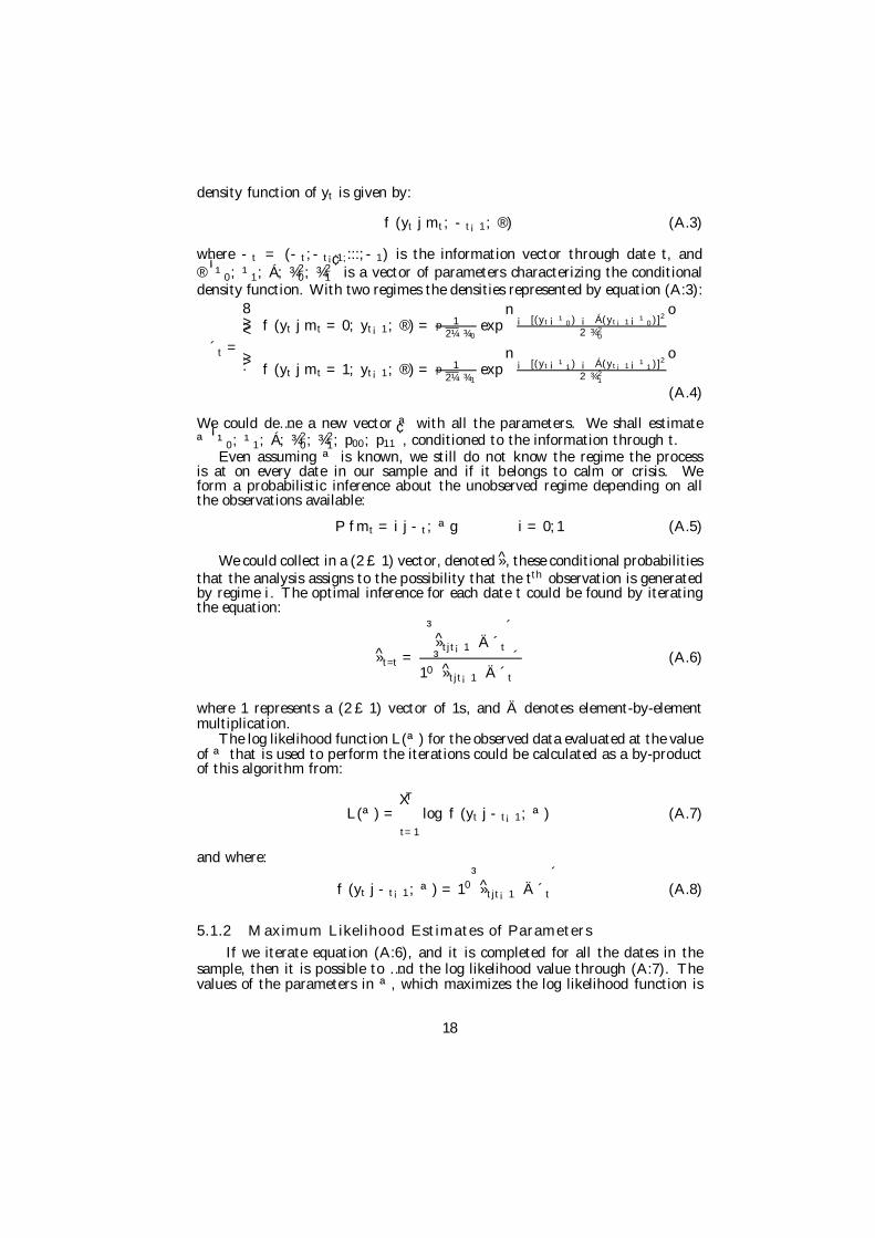
density function of yt is given by:

f (yt j mt; ­t¡1; ®) (A.3)

where ­t = (­t;­t¡1;:::;­1) is the information vector through date t, and®

¡¹0; ¹1; Á; ¾2

0; ¾21

¢is a vector of parameters characterizing the conditional

density function. With two regimes the densities represented by equation (A:3):

´t =

8>><>>:

f (yt j mt = 0; yt¡1; ®) = 1p2¼ ¾0

expn

¡ [(yt¡¹0) ¡ Á(yt¡1¡¹0)]2

2 ¾20

o

f (yt j mt = 1; yt¡1; ®) = 1p2¼ ¾1

expn

¡ [(yt¡¹1) ¡ Á(yt¡1¡¹1)]2

2 ¾21

o

(A.4)

We could de…ne a new vector ª with all the parameters. We shall estimateª

¡¹0; ¹1; Á; ¾2

0; ¾21; p00; p11

¢, conditioned to the information through t.

Even assuming ª is known, we still do not know the regime the processis at on every date in our sample and if it belongs to calm or crisis. Weform a probabilistic inference about the unobserved regime depending on allthe observations available:

P fmt = i j ­t; ªg i = 0; 1 (A.5)

We could collect in a (2 £ 1) vector, denoted »̂, these conditional probabilitiesthat the analysis assigns to the possibility that the tth observation is generatedby regime i. The optimal inference for each date t could be found by iteratingthe equation:

»̂t=t =

³»̂tjt¡1 Ä ´t

´

10³»̂tjt¡1 Ä ´t

´ (A.6)

where 1 represents a (2 £ 1) vector of 1s, and Ä denotes element-by-elementmultiplication.

The log likelihood function L(ª) for the observed data evaluated at the valueof ª that is used to perform the iterations could be calculated as a by-productof this algorithm from:

L(ª) =TX

t=1

log f (yt j ­t¡1; ª) (A.7)

and where:

f (yt j ­t¡1; ª) = 10³»̂tjt¡1 Ä ´t

´(A.8)

5.1.2 Maximum Likelihood Estimates of ParametersIf we iterate equation (A:6), and it is completed for all the dates in the

sample, then it is possible to …nd the log likelihood value through (A:7). Thevalues of the parameters in ª, which maximizes the log likelihood function is

18

obtained by numerical optimization using, in our case, the Newton-Raphsonalgorithm.23 The results are shown in table1 and the following …gure representsdaily interest rate di¤erential between Spain and Germany during the sampletime.

-0.35

0.65

1.65

2.65

3.65

4.65

5.65

6.65

7.65

8.65

19/06/1989 19/06/1990 19/06/1991 19/06/1992 19/06/1993 19/06/1994 19/06/1995 19/06/1996 19/06/1997 19/06/1998

Interest Rate Differential

Daily Interest Rate Di¤erential between Spain and Germany[1989/06/19 1998/12/30]

23 [17, Hamilton, 1994, ch. 5, p. 133-142]

19

Readjustment Probability [Peseta/Deutsche Mark Exchange Rate]

0

0.1

0.2

0.3

0.4

0.5

0.6

0.7

0.8

0.9

1

19/06/1989 19/06/1990 19/06/1991 19/06/1992 19/06/1993 19/06/1994 19/06/1995 19/06/1996 19/06/1997 19/06/1998

Probability [et, (emáx - et), (et - ct), st]

0

0.1

0.2

0.3

0.4

0.5

0.6

0.7

0.8

0.9

1

19/06/1989 19/06/1990 19/06/1991 19/06/1992 19/06/1993 19/06/1994 19/06/1995 19/06/1996 19/06/1997 19/06/1998

Probability [et, (emáx - et), (et - ct)]

0

0.1

0.2

0.3

0.4

0.5

0.6

0.7

0.8

0.9

1

19/06/1989 19/06/1990 19/06/1991 19/06/1992 19/06/1993 19/06/1994 19/06/1995 19/06/1996 19/06/1997 19/06/1998

Probability [(emáx - et), st]

0

0.1

0.2

0.3

0.4

0.5

0.6

0.7

0.8

0.9

1

19/06/1989 19/06/1990 19/06/1991 19/06/1992 19/06/1993 19/06/1994 19/06/1995 19/06/1996 19/06/1997 19/06/1998

Probability [(emáx - et)]