DOCUMENTOS DE ECONOMIA YFINANZAS INTERNACIONALES

Asociación Española de Economía y Finanzas Internacionales

http://www.fedea.es/hojas/publicaciones.html

DOMESTIC AND FOREIGN PRICE-MARGINALCOST MARGINS: AN APPLICATION TO

SPAIN MANUFACTURING FIRMS

Lourdes Moreno MartínDiego Rodríguez Rodríguez

September 2000

DEFI 00/03

Domestic and foreign price-marginal cost margins:

an application to Spanish manufacturing firms

Lourdes Moreno MartínDiego Rodríguez Rodríguez

Universidad Complutense de Madrid y PIE-FEP

Address:

Lourdes Moreno MartínFundación Empresa PúblicaC/ Quintana, 2, 3ª28008 Madrid

Tel.: 91 548 83 51E-mail: lmoreno@funep.es lmoreno@ccee.ucm.es

1

Abstract

The objective of this paper is to analyse the differences in price-marginal cost margins of the export

and domestic markets by the estimation of a multiproduct cost function. We apply this method to a

panel of Spanish export manufacturing firms from the period 1990-1997. Some results emerge from

the estimations. First, price-marginal cost margins in domestic markets are larger than foreign margins

throughout the period. Second, price-marginal cost margins are procyclical in the domestic market but

there is no evidence of this behaviour in the foreign markets. Third, there is no evidence that export

firms used the devaluation of the currency to increase their margins. Finally, price-cost margins reveal

some degree of heterogeneity across industries in both markets.

Keywords: Marginal cost, price-cost margins, translog cost function, export firm.JEL Classifications: F12, L60, L13

Resumen

El objetivo del trabajo es analizar si existen diferencias en los márgenes precio-coste marginal en los

mercados doméstico y exterior de las empresas manufactureras exportadoras españolas durante el

período 1990-97. La estimación de una función de costes variables multiproducto permite obtener los

costes marginales de las ventas dirigidas a cada destino y calcular los márgenes de ambos mercados.

Los resultados que se derivan se resumen a continuación. En primer lugar, los costes marginales

asociados a las exportaciones son mayores a los de las ventas dirigidas al mercado interior. Aunque

existe una gran heterogeneidad entre empresas, los márgenes interiores son superiores a los del

mercado de exportación. En segundo lugar, el margen doméstico es procíclico pero no existe evidencia

de este comportamiento en el mercado exterior. En tercer lugar, las empresas exportadoras no han

aprovechado las devaluaciones de la peseta en 1992 y 1993 para incrementar sus márgenes en los

mercados de exportación. Por último, existe una gran heterogeneidad en los márgenes domésticos e

interiores entre industrias.

2

I. Introduction

Some classical studies of Industrial Economics have analyzed the effect of import and

export activities on the total profitability of industries. With respect to imports, if there is no

relationship between domestic and foreign firms, import penetration (defined as imports over

total sales) should have a negative effect on total profitability. Most empirical papers work

with this assumption and find supporting evidence1. However, if collusive behavior between

domestic and foreign firms is assumed, import penetration does not imply more competition.

In this case, positive or ambiguous effects could be found2.

The influence of exports on profitability and domestic competition is less

straightforward. The overall effect depends on the conditions under which goods are traded in

the world market relative to the domestic situation. One of the variables affecting relative

margins is the demand elasticity of both markets. In the context of homogeneous products, it

is normally assumed that world demand elasticity is bigger than domestic demand elasticity,

supporting a larger domestic price-cost margin relative to the foreign margin. An extreme

situation would be where producers are confronted with a perfectly elastic demand. In this

case, international price equals export price (corrected by the exchange rate if it is invoiced in

domestic currency). However, if differentiated products are assumed, it is possible to find that

domestic exporters sell to specific fringe demands of foreign countries with demand less

elastic than the domestic demand. If the domestic firm is not a price taker in the international

1 See, for example, Lyons (1981), Jacquemin (1982), Geroski (1982) and, for Spain, Mazón (1993).Stalhammar (1991) also finds empirical support that imports have a negative influence on the degree ofimplicit collusion on the domestic market.2 Fariñas and Huergo (1993) consider the possibility of collusive behavior between Spanish and foreign firms.In their estimates with Spanish data up to 1986, they found that import penetration of the OCDE positivelyaffects profitability, while imports from the rest of the world affect it negatively. Pearce de Azevedo (1996 and1998) finds similar results using data up to 1990. The import rate tends to depress the margins in more

3

markets, it is possible to find market power abroad as well as in the home market, and in this

sense export profit can be higher than domestic profit. In addition to the differences in

demand elasticities and competition environment, differences in marginal costs could justify

different margins between both markets. Even in the context of a homogeneous product,

variable (e.g., transport) or sunk (e.g., export channels) costs related to exports could easily

justify such differences.

Empirical evidence of the effect of exports on profitability is inconclusive. Caves,

Porter and Spence (1980) find that exports reduce the profitability of industry, while Geroski

(1982) finds a positive effect of the export rate on the margin. For Swedish industry,

Stalhammar (1991) obtains a non-significant effect of export rate on industry profitability.

However, exports have a negative influence on the degree of implicit collusion in the

domestic market. These inconclusive results also appear for the Spanish economy. In

Maravall and Torres (1986), the export rate negatively affects profitability (measured as cash

flow over sales), but it is non-significant. Pearce de Azevedo (1996 and 1998) finds a positive

and significant effect of the export rate on profitability when macroeconomic effects and

potential endogeneity are not considered. However, when both facts are considered, the

variable is not significant and even ends up changing to negative.

An alternative line of work differing from previous empirical work in industrial

economics was called New Industrial Economics by Bresnahan (1989). Instead of studying

the determinants of industry profitability by the estimation of price-cost margin equations, it

analyzes the price-cost margins directly from a structural econometric model. To do that, a

concentrated industries, but the average impact of imports tends to be insignificant.

4

cost or production function together with margin equations are estimated. It also allows us to

determine additional parameters like demand elasticity, pricing behavior and firm

interdependence through conjectural elasticity3.

Following that line, Bernstein and Mohnen (1991) and Bughin (1996) have estimated

the price-cost margin in some industries, differentiating between export and domestic

markets. Bernstein and Mohnen (1991) estimate a model for oligopolistic industries where

firms distinguish between output sold domestically and exported. They work with sectoral

data and their model is applied to Canadian non-electrical machinery, electrical products and

chemical products industries. Departing from a multiproduct cost function, they estimate the

degree of oligopoly power in each industry, as well as the elasticities of both demands,

through the specification of the share of the labor cost to the variable cost, the foreign and

domestic revenues over the cost, and the two inverse product demand functions. They find

that the degree of oligopoly power differs between domestic and foreign markets.

Bughin (1996) works with firms’ data and assumes monopolistic competence. The

different price-cost margins are explained by the different demand elasticities in each market

taking into account the possibility that short-run capacity restrictions affect pricing decisions.

He applies his model to a panel of Belgian firms in the Chemical and Electrical and Electronic

products, finding that monopoly power over export markets is small.

Following Bernstein and Mohen (1991) and Bughin (1996), our paper evaluates the

3 The first papers worked in a static context (see, for example, Appelbaum (1982) and Roberts (1984)). Later,dynamic considerations were included (see, for example, Morrison (1988) and, for Spain, Huergo (1998) andFariñas and Huergo (1999)).

5

domestic and foreign price-cost margins of Spanish export firms for the period 1990-97.

That period was especially relevant for Spanish and other European economies, due to the

turbulence in the EMS and strong changes in the economic cycle. Both circumstances should

have affected the competitive position of export firms. Though some evidence exists that such

events affect export margins (see, for example, Gordo and Sánchez Carretero (1997)), it is

always based on macroeconomic data, mainly the evolution of aggregate price indexes, and

not on firm data.

We are interested not only in testing the differences in margins related to export and

domestic activities, but also analyzing how the evolution of domestic and foreign demand and

the evolution of nominal exchange rate affect both margins. To answer these questions, we

follow a two-step approach. Firstly, we estimate a multiproduct cost function, obtaining

different marginal costs associated to products sold in domestic and export markets.

Secondly, departing from these estimated marginal costs, we calculate the price-marginal cost

margins separately for each market.

The rest of the paper is as follows: In section II, the theoretical framework is

explained. In section III, we present the estimate of the multiproduct cost function and the

foreign and domestic margins. Finally, section IV presents the conclusions.

The results obtained indicate that the average marginal costs of the production sold

in export markets are greater than those of the production sold in domestic markets. At the same

time, the price-marginal cost margin in the export market is smaller than in domestic markets. We

found that price-cost margins are procyclical in the domestic market, but there is no evidence of

6

this behaviour in the foreign markets. Additionally, the evolution of the nominal exchange rate

presents the expected sign in the explanation of the domestic margin but it is non-significant. There

is no evidence that firms used the devaluations of the peseta in 1992 and 1993 to increase the

margins in export markets. Finally, price-cost margins reveal some degree of heterogeneity across

industries in both markets but the margin is bigger in the domestic in the most industries.

7

II. Theoretical benchmark and econometric specification

We consider a firm selling a product in two different markets, home and foreign,

characterised by imperfect product competition. The price-cost margins in both markets can

be expressed, as usual, from4:

Pj (1-µj) = Cj´ j=d,x [1]

where Cj´ is the marginal cost in each market, pj is the price of sales in domestic (d) and

foreign (x) markets and µj is the price-marginal cost margin in each market.

Of course, if µj is expressed in terms of the demand elasticity and conjectural

variations of the firm, the expression [1] can be interpreted as the first order condition of the

joint profits maximisation of a firm selling in domestic and foreign markets and without

capacity restrictions. With perfect competition, µj is equal to zero and price is equal to

marginal cost. If the firm faces monopolistic competition in each market, µj is equal to the

inverse of demand elasticity. If the firms operate in an oligopolistic context, µj reflects not

only demand elasticity but also strategic behaviour of firms. In this context, µj can be

expressed as λji/εj, where ) /( ylnyln = i

jij

i

ij ∂∂λ ∑ is the conjectural elasticity of firm i in

market j, and εj is the demand elasticity in that market. Bernstein and Mohnen (1991) assume

that the firms work in an oligopolistic context and evaluate both parameters separately5.

However, we do not assume any predetermined context of imperfect competence, so that the

4 We omit the superscript about firms for simplicity.

8

parameter µj measures the market demand elasticity as well as the strategic behaviour of rival

firms.

Information about marginal costs and the level of prices in each market are required to

obtain specific margin (µ) for each j market in the expression [1]. The latest information is

scarcely available. However, expression [1] can be rewritten as:

xd, = j Yln

Cln = ) - (1

CYP

jj

jj

∂∂

µ [2]

This identity has some advantages with respect to the identity [1]. To estimate the

price-marginal cost in each market, the prices of sales in each market are not necessary; it is

enough to have the real sales sold in each market. Therefore, only a market-specific index

price is required6.

To estimate the identity [2], it is necessary to obtain the elasticity of cost with respect

to production sold in both markets. We assume a short-term context where capital stock is

considered as a fixed factor. The variable cost function is defined as:

C = C (Pf, Yj, K,t) [3]

5 To do that, they include the inverse demand functions in the set of equations to estimate, identifying theprice elasticity.6 The information given by the ESEE allows us to calculate prices index (see Appendix 1).

9

where Yj is the vector of output sold in domestic (d) and foreign (x) markets7, Pf is a vector

of prices of the variable factors (labour (L) and intermediate inputs (M)), K is capital stock

and t is a time trend approximating the technology state. All firms in the industry face the

same variable factor prices. The cost function has the usual properties: it is increasing in

variable factor prices and outputs, and it is also homogeneous of degree one in the factor

prices.

Two outputs enter into the cost function because, even if they are physically alike,

variable costs include some costs that can differ among the outputs. The most striking of

these are transport costs, which are clearly related to distance and, therefore, assumed to be

larger in sales in foreign markets. Accordingly, other costs, such as advertising costs, can be

positively related to sales in non-domestic markets. However, no other variable costs

associated to exports, such as sunk costs for establishing delivery channels in export markets,

are considered in this short-term benchmark.

Following the usual line in this literature, a multiproduct translog function is

specified8. As it is known, the translog function is a more flexible way to specify a cost

function than other alternatives, such as a Cobb-Douglas function, and does not impose the

restrictions of homotheticity and separability. The translog function is written as:

7 We only have information about the total production of firms. Foreign production is approximated byexports. Domestic production is approximated by total sales minus exports.8 An alternative specification is the generalized translog function, which would permit us to work withobservations equal to zero (Caves et al (1980)). However, our interest in this work lies in firms operatingsimultaneously in both markets.

10

( ) ( ) ( ) ( ) ( )

( ) ( ) ( ) ( ) ( ) ( )[ ]

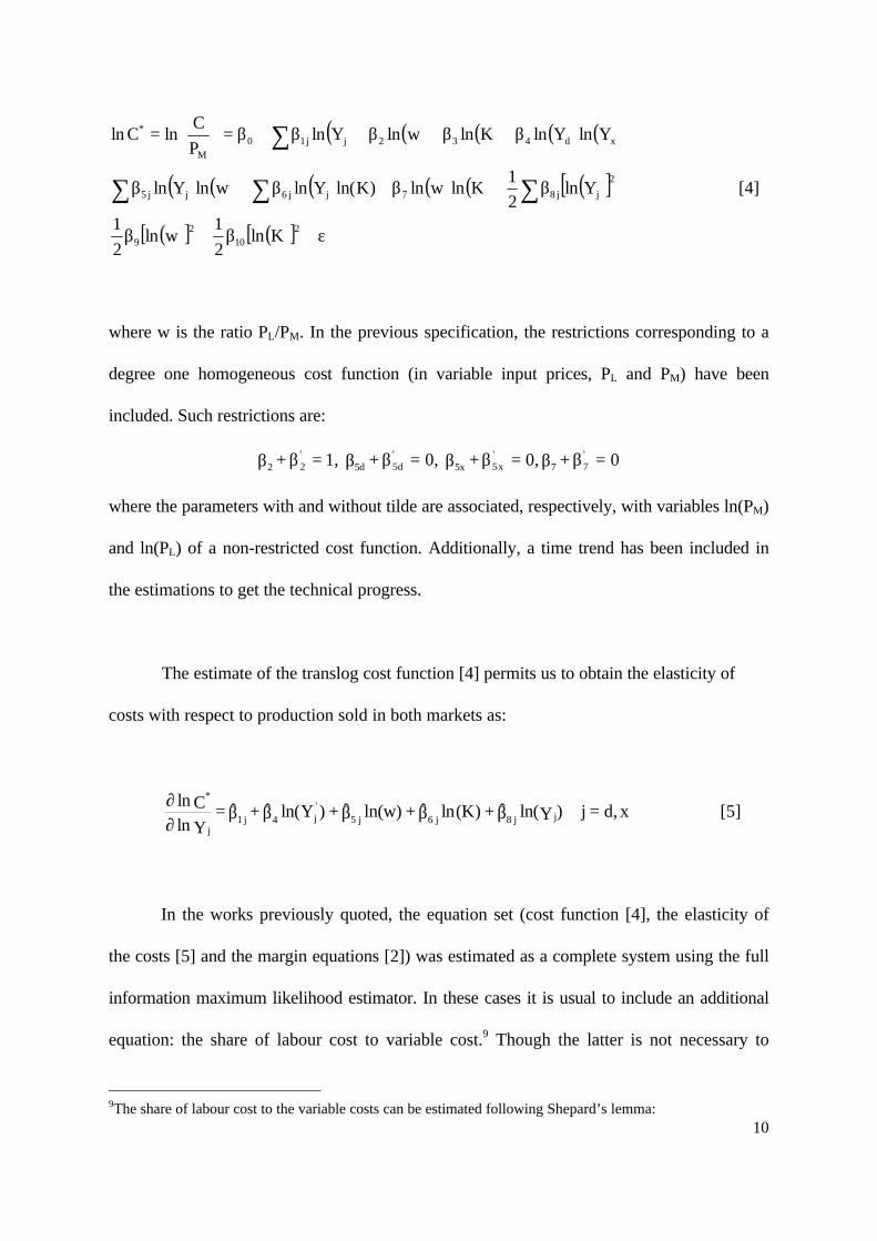
( )[ ] ( )[ ] ε+β+β

+β+β+β+β

+β+β+β+β+β=

=

∑∑∑

∑

210

29

2

jj87jj6jj5

xd432jj10M

*

Kln2

1wln

2

1

Yln2

1Klnwln)Kln(YlnwlnYln

YlnYlnKlnwlnYlnP

ClnCln

[4]

where w is the ratio PL/PM. In the previous specification, the restrictions corresponding to a

degree one homogeneous cost function (in variable input prices, PL and PM) have been

included. Such restrictions are:

0=+ 0,=+ 0,=+ 1,=+ '77

'x55x

'd55d

'22 ββββββββ

where the parameters with and without tilde are associated, respectively, with variables ln(PM)

and ln(PL) of a non-restricted cost function. Additionally, a time trend has been included in

the estimations to get the technical progress.

The estimate of the translog cost function [4] permits us to obtain the elasticity of

costs with respect to production sold in both markets as:

xd,=j )Yln( ˆ + )(Kln ˆ + ln(w) ˆ + )Yln( ˆ + ˆ = YlnCln

jj8j6j5'j4j1

j

*

βββββ∂∂

[5]

In the works previously quoted, the equation set (cost function [4], the elasticity of

the costs [5] and the margin equations [2]) was estimated as a complete system using the full

information maximum likelihood estimator. In these cases it is usual to include an additional

equation: the share of labour cost to variable cost.9 Though the latter is not necessary to

9The share of labour cost to the variable costs can be estimated following Shepard’s lemma:

11

identify the parameters, it is included in the set of equations for efficiency’s sake. However,

in this work a different perspective is used. Firstly, we estimate the variable cost function

using instrumental variables. Taking these results, we calculate ∂ ln C* / ∂ ln Yj for each firm

in both markets. From the estimated elasticities, the identity [2] permits us to calculate the

price-marginal cost margins in each market.

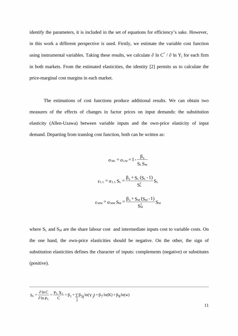
The estimations of cost functions produce additional results. We can obtain two

measures of the effects of changes in factor prices on input demands: the substitution

elasticity (Allen-Uzawa) between variable inputs and the own-price elasticity of input

demand. Departing from translog cost function, both can be written as:

where SL and SM are the share labour cost and intermediate inputs cost to variable costs. On

the one hand, the own-price elasticities should be negative. On the other, the sign of

substitution elasticities defines the character of inputs: complements (negative) or substitutes

(positive).

(w)ln9 + (K)ln 7 + )Y j(ln 5jj

+ = CX P =

Pln

Cln = S 2

LL

LL βββ∑β

∂∂

S S

1)-S( S + = S =

S S

1)-S( S + = S =

SS

- 1 = =

M2M

MM9MMMMM

L2L

LL9LL LL L

ML

9LMML

βσε

βσε

βσσ

12

Finally, to evaluate the scale elasticity in a short-term context and a multiproduct

function, we use, following Caves et al. (1981):

A value of RS equal (smaller, bigger than) to one reflects constant (decreasing, increasing)

returns to scale.

Yln/Cln

lnK/Cln - 1 = SR

j*

j

*

∂∂∂∂

∑

13

III. Empirical results.

The sample used consists of a panel of Spanish manufacturing exporting firms for the

period 1990-1997. The variables were obtained from the Encuesta sobre Estrategias

Empresariales (ESEE, Survey on Business Strategies). This survey is carried out yearly by

the Spanish Ministry of Industry and the Fundación Empresa Pública. The population

considered in this survey is about 2000 manufacturing firms that have ten or more employees.

We work with a balanced panel of exporting firms in the period 1990-97. Forty

percent of small firms (less than 200 employees) exported during this period. For larger firms,

(more than 200 employees) this percentage surpasses 80%. We have excluded firms exporting

less than 5% or more than 95% of their sales more than four years. Additionally, we lose

some firms that do not give enough information to calculate the capital stock and price

variations needed in order to obtain the price index of intermediate inputs and the price

indexes of domestic and foreign markets. The number of available firms, after those with

incomplete information were dropped, is 331. We do not have enough information to

estimate the price-cost margins for specific industries, and for this reason we work with the

overall industry. However, industry effects will be included in the estimations in order to

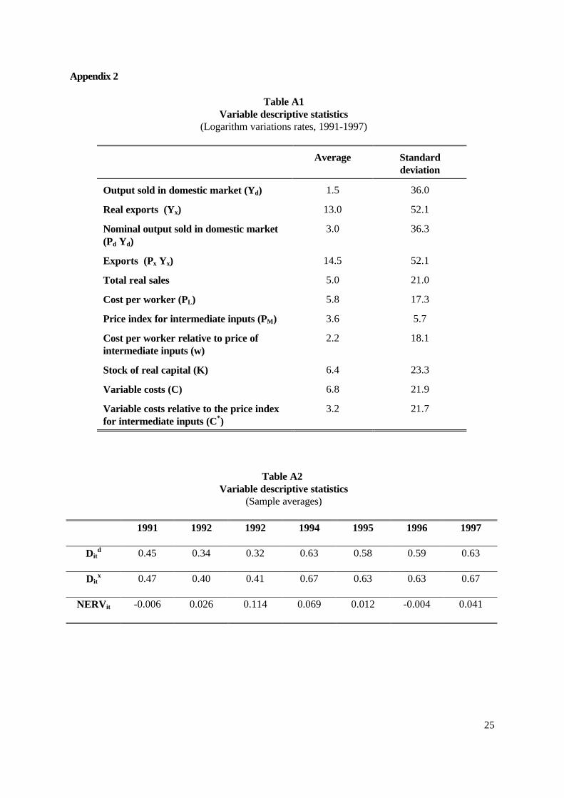
capture cross-industry differences. Information about the main descriptive statistics is shown

in Table A1 of Appendix 2.

Note that though some of the surveyed firms are integrated in foreign-owned groups,

especially in the case of larger firms, we only pay attention to Spanish firms, not to the overall

group of firms. Therefore, our cost measurement is not biased by the usual behavior of

14

multinational firms that produce in several countries. Although the measurement of imported

intermediate inputs would be affected if transfer pricing practices were important, it does not

affect the differences in margins in both markets.

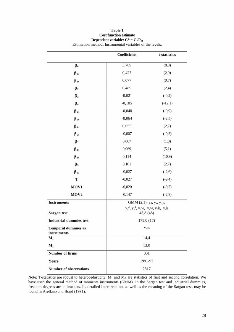
Table 1 shows the level estimations of the translog cost function [4] by instrumental

variables. We assume that firms are price-takers in variable input markets, so variable input

prices are considered exogenous. However, endogeneity in sales in both markets is assumed.

To estimate this equation, we use the Generalised Method of Moments (GMM) procedure

proposed by Arellano and Bond (1991). The estimation is carried out instrumenting the

variables shown in Table 1 at t with their cross-section lagged values at t-2. The identification

condition depends on whether lagged values of the endogenous variables are valid

instruments. The Sargan test of overidentifying restrictions, a test of instrument validity, is

presented at the bottom of the columns and the validity of instruments is accepted. The

residual autocorrelation tests m1 and m2 denote correlation in the level estimate. We think that

this correlation is caused by the existence of individual firm heterogeneity. When we

produced a first difference estimate, the values of the m statistics denoted the presence of an

MA(1) process, as we can expect after taking differences of uncorrelated residuals.

Unfortunately, the marginal costs predicted by the first difference estimation produce

unacceptable domestic and foreign margins.

Industrial dummies are included to try to capture some specific industry effects

common of firms10. The Wald test at the bottom of Table 1 confirms their significance. The

10 18 manufacturing industries have been introduced.

15

estimation also includes a time trend11, whose associated parameter can be seen as technical

progress and, given that a cost function is being estimated, the expected sign is negative. The

estimated value in Table 1 is –2.7.

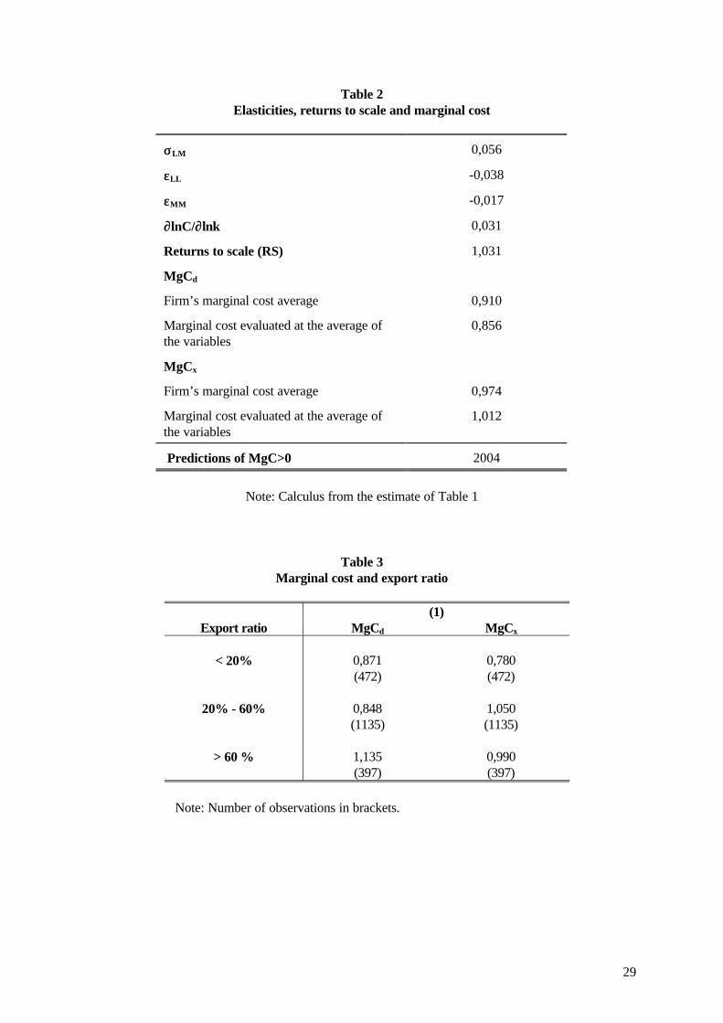
Table 2 presents the Allen-Uzawa partial elasticities of substitution, the own-price

elasticities of demand, returns to scale economies, and marginal costs derived from level

estimations. We have used the sample average of the share of labour cost (SL=0.31) and

intermediate inputs (SM=0.69) to total variable costs to calculate the elasticities. As can be

seen, price elasticities are negative and the inputs (labour and intermediate materials) are

substitutes. The scale elasticity value is one, so firms seem to operate under constant returns

to scale.

The estimate of the translog cost function permits us to obtain individual predictions

of the ∂lnC*/∂lnYj (see expression [5]). More than eighty-four percent of the predictions are

positive, while the majority of negative predictions are very near zero. Those negative

predictions are from firms with a very low share of domestic sales or exports with respect to

total sales, less than 10%. Insofar as this feature is more common in the case of sales in

export markets than in domestic markets, there is a larger number of negative predictions of

marginal costs linked to export activity.

The marginal costs for each firm have been evaluated as ∂C/∂Yj = C ∂lnC* / Yj ∂lnYj.

Table 2 shows the predicted values for the subsample with positive predictions, and for the

overall sample. The average marginal cost has been calculated in two ways. In the first one,

11 Some authors include the time trend multiplied by explicative variables in translog functions. In our case

16

we calculated the sample average of the individual marginal cost for each firm. In the second

one, the expression [5] is evaluated in the average of the variables. The predictions show, as

was expected, a larger average marginal cost for sales in export markets. However, there is a

non-linear relationship between the export ratio (proportion of output sold in the foreign

market) and the differences in marginal costs. As can be seen in Table 3, firms who sell a

similar proportion of their output in both markets present a larger average marginal cost in

the export market. This does not happen, however, for firms which sell most of their output

in one of the markets, and which represent a small proportion of the sample.

From expression [2] and the individual predictions of the elasticity of the cost with

respect to the real sales in each market (expression [5]), it is possible to calculate the

individual price-cost marginal. To do that, we have restricted the sample to the positive

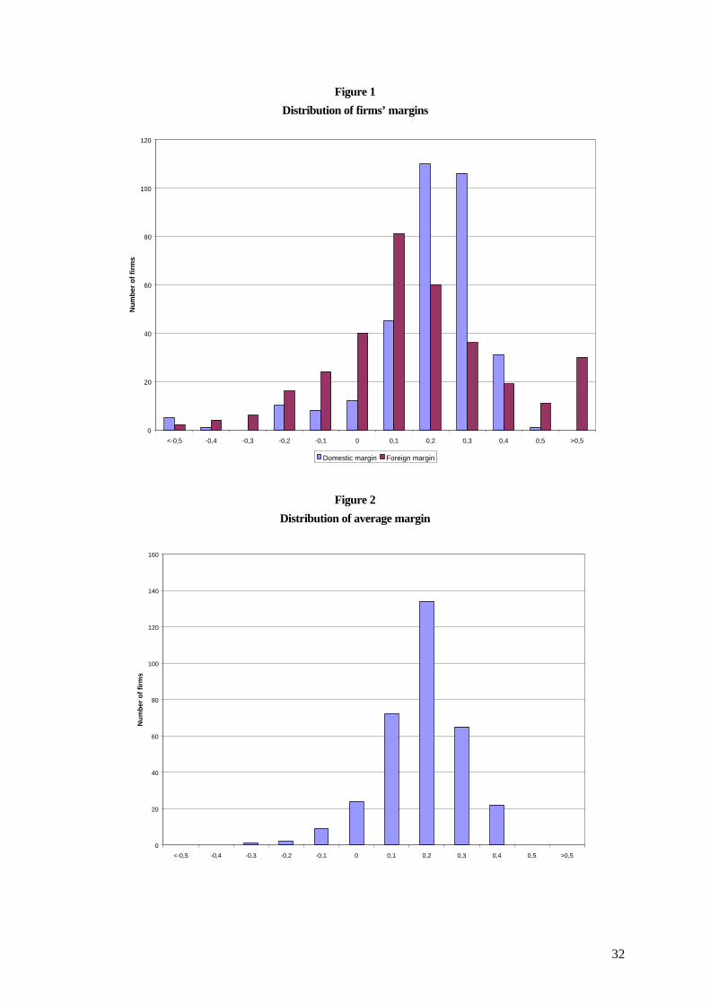
predictions of the marginal cost. Figure 1 shows the distributions of the average domestic and

foreign margins for the period 1991-1997 for each firm. Both distributions are slightly skewed

with a big proportion of firms on the right tail. Comparing the domestic and the foreign price-

cost marginal margins, there is a bigger proportion of firms with positive margins in the

domestic market. More than 65% of firms present a domestic margin between 0.1 and 0.3.

However, there are some firms (about 7%) which present a higher foreign margin (more than

0.5) than domestic price-cost marginal margin.

Figure 2 shows the distribution of the average margin in both markets, weighting the

foreign and the domestic margin for the export ratio (exports over sales) and domestic sales

ratio (one minus export ratio) respectively. The distribution is skewed with almost all the

firms on the right tail. Only 11% of individual firms’ average margins fall below zero. The

these variables are non-significant.

17

results are consistent with international studies that examine the price-marginal cost margin

with firms’ data (see, for example, Nishimira et al. (1999)).

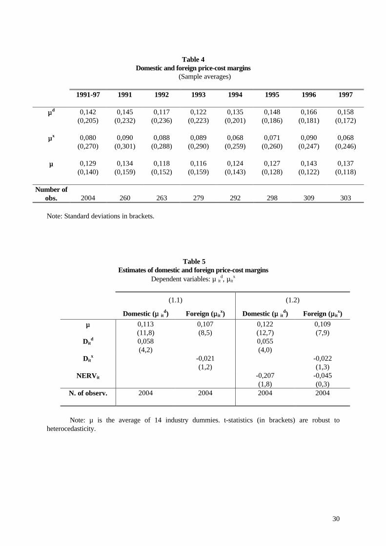
Table 4 presents the sample average of the margins for the whole period and for each

year. Although there is a huge heterogeneity between firms, the average price-cost margin of

firms in foreign markets was smaller than the average price-cost margin in the domestic

markets in the entire period. It seems that the domestic price-cost marginal margins are

procyclical with the smallest value in 1992, but there is no evidence of this behaviour in the

price-cost margins in the foreign market. This behaviour in the foreign market can be affected

by the evolution of the nominal exchange rate. As can be seen in Figure 3, the average margin

is procyclical with the smallest value in 1993.

The cyclicality of the margin has been intensely discussed in the literature. To give more

information about that, Table 5 presents some estimations of the margin for both markets,

considering only the positive predicted values of marginal costs. The margins have been

parameterised in two alternative ways. In the first one, the parameterization takes into account

the heterogeneity of firms over different activities, which also have a different behavior over

the business cycle. These industry characteristics are related to demand elasticity.

dit

d0

ds

dit D+ = βµµ , x

itx0

xs

xit D + = βµµ [6]

where µs are fourteen industry dummies and Ditd and Dit

x are individual indicators of the

business cycle for each firm in domestic and foreign markets respectively. An increase in

18

these indicators means an improvement in the market conditions of firms. Table A2 of

Appendix 2 presents the sample averages of these variables. The second parameterization also

takes into account the possible effect of the variation of the nominal exchange rate in the

price-marginal cost margin of the firms (NERVit).

itd1

dit

d0

ds

dit NERV D+ = β+βµµ , it

x1

xit

x0

xs

xit NERVD + = β+βµµ [7]

where NERVit is an individual indicator of the evolution of the nominal exchange rate. An

increase of this indicator means a devaluation (or depreciation) of our currency (see Table A2

of Appendix 2).

The second and third columns of Table 5 present the estimate using the first

parameterisation12. As was said before, the average price-cost margin of firms in foreign markets

was smaller than the price-cost margin in the domestic markets for the whole period. The

coefficient for the individual indicator of the business cycle (Ditd) presents the expected sign –

positive- in the estimate of the domestic margin. However, it presents an unexpected sign in the

estimate of foreign margin, although it is non-significant. It seems, therefore, that domestic price-

marginal cost margins are clearly procyclical, but there is no evidence of this behaviour in the

price-cost margins in foreign markets. Figure 4 plots the domestic (foreign) business cycle

indicator and the predictions of both price-marginal cost margins for the estimate of Table 5. As

can be seen, the behaviour of domestic price-cost margin follows the evolution of the domestic

cycle indicator. With respect to the foreign market margin, it increased in 1992 and 1993 (the

12 Table 5 presents pool estimates. We have also considered that the individual effects are correlated with theexplanatory variables. The Haussman test cannot reject the null hypothesis of no correlation. The randomeffects estimation is quite similar to the pool estimation and for this reason we only present the latter.

19

years of the devaluation of the peseta) although the foreign cycle indicator decreased in these

years.

Columns four and five of Table 5 present the estimate using the second parameterisation.

As can be seen, the parameter associated to NERVit presents the expected sign (negative) in the

estimate of domestic margin although it is non-significant. The depreciation of our currency

increases the prices of imported inputs and reduces the domestic margin. However, it presents an

unexpected sign in the estimate of the foreign margin although it is non-significant. These results

seems to indicate that, at least in the long term, Spanish export firms did not use the devaluations

of our currency in 1992 and 1993 to increase the margins in exports markets. It would indicate a

high degree of exchange rate pass through to export price (in foreign currency) and/or that the

effect of devaluations on imported intermediate input prices partially absorbed the positive short-

term effect of devaluations on export prices. In that sense, this evidence is not so optimistic about

the recovery of export margins after the devaluations of the peseta in 1992-1993 as the previous

evidence, which had departed from an industry perspective (Gordo y Sánchez Carretero (1997)).

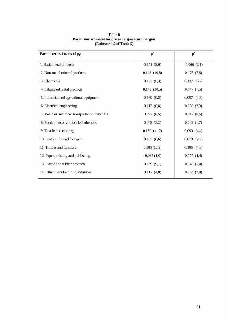
The parameterisation of margins allows us to obtain industry-specific effects, µs (see

expression [6] and [7]). The parameters estimated from the industries’ price-cost margins for

estimation (1.2) of Table 5 are shown in Table 6. The estimates reveal some degree of

heterogeneity in price-cost margins across different manufacturing industries, bigger in the

domestic than in the foreign market. The domestic margin is significantly greater than zero in most

industries, suggesting that firms possess significant domestic market power. The foreign margin is

smaller than 0.1 in six of the fourteen industries, suggesting smaller foreign market power. Paper,

printing and publishing and other manufacturing industries are the exceptions, a with smaller

20

margin in the domestic market the entire period.

21

IV. Conclusions

It is usually assumed that the differences in the competitive environment or in the evolution

of the demand among markets, added to the specific disturbing effect of exchange rate variations,

could generate differences in the levels and evolution of the price-cost margins between domestic

and foreign markets. However, an additional effect could be derived from the existence of different

marginal costs associated to sales in distinct geographical markets. In this paper we calculate

margins for each market, taking into account such differences. The method used is adapted to the

information usually available in firm surveys.

The obtained results indicate that Spanish manufacturing export firms have larger average

marginal costs for exports than for sales in domestic markets. In a short-term context, with fixed

capital stock, such differences should be mainly due to the effect of transport costs, though other

effects could play a role (e.g., differences in marketing costs associated to export markets). A

more precise test would require some measurement of transport costs, data which is scarcely

available13.

Additionally, the estimated price-cost margins differentiated by markets show that the

average margin in export markets was smaller than in domestic markets throughout the period.

Besides, the evolution along the period was distinct. The domestic price-marginal cost margin is

procyclical: the margin fell until 1993 and increased in the other years. At the end of the period,

domestic margins were bigger than those in 1991. We do not find evidence of procyclical

behaviour or a significant effect of nominal exchange rate variations on export margins. The result

is a slight process of convergence between both margins until 1993. However, the domestic price-

22

cost margin still continued behind the foreign margin in 1997, and the differences even increased.

The average margin is procyclical, according to previous studies of the Spanish economy (see, for

example, Fariñas y Huergo (1999)) and with international studies examining the cyclicality of

margin with firms’ data (see, Nishimira et al. (1999)).

These results complement those obtained in the context of “Pricing to Market” literature.

In that case, non-complete exchange rate pass through and price stickiness (in local currency)

suggest that export margins partially absorb the exchange rate fluctuations. However, as Golgberg

and Knetter (1997) have pointed out, the difficulty in measuring marginal costs can bias the results.

Though Knetter (1993) proposed a simple empirical way to avoid it, it is based on some crucial

assumptions, such as homogenous variations of marginal costs across firms and industries, and is

only valid for cross-sectorial comparisons of prices. The results of this paper confirm such

variations in export margin, but suggest that the results in PTM literature could be overestimating

the effects of exchange rate variations on export margins, as they do not properly consider the

marginal costs variations.

13 The evidence obtained by some authors points out the relevance of considering them in the case of some keyprediction of industrial organisation literature (see Newmark (1998)).

23

Appendix 1: Variable definitions.

C (Variable costs): The sum of intermediate consumption (raw materials purchases, energy and fuel costs

and other external services) plus labour costs minus the stock variation.

W (Cost per worker relative to price of intermediate inputs): PL/PM, where:

PM (Price index for intermediate inputs): It is calculated as a Paasche index, weighting the price variations

of raw materials, energy and services purchased of surveyed firms.

PL (Cost per worker): Labour cost divided by the average workers of the firm during the year.

Yx (Output sold on the export market): It is calculated deflating nominal exports by export price (Px).

Yd (Output sold on the domestic market): It is calculated deflating nominal domestic sales by domestic

price (Pd). Domestic sales are the total sales of the firm minus its exports.

Pd and Px (Domestic and foreign prices): The surveyed firms give annual information about markets

served (up to five), identifying their relative importance (in percentage) in total sales of the firm.

Additionally, each firm identifies the geographical area and the variation of price with respect to the previous

year. This information allows us to calculate a price index for each market, using the proportions with

respect to total sales as weighting.

K (Capital stock): It is net stock of capital for equipment in real terms. It is calculated using the perpetual

inventory formula:

24

t1t

t1t I

P

PK)d1(K +−=

−−

where P is the price index for equipment, d are the rates of depreciation, and I is the investment in

equipment. For details about the elaboration of this variable, see Martín and Suárez (1996).

Ditd, Dit

x (Individual indicator of business cycle for each firm in domestic and foreign market): In the

ESEE survey, each firm identifies the behaviour of market demand during one year with respect to the

previous years according to three different categories: expansion, stability and recession. A value of 1, 2 and

3 is assigned respectively to each category. The domestic and foreign indexes are constructed weighting the

previous values over all domestic and foreign markets defined by the firm. The weights are the proportion of

sales in each market with respect to total sales.

NERVit: In the ESEE survey, export firms identify the export destiny. They distinguish between the

European Union, the rest of the OCDE and the rest of the world. An individual nominal exchange rate has

been calculated weighting the Spanish nominal exchange rate with respect to these areas. The weights are

the proportion of exports sold in each area with respect to total exports.

25

Appendix 2

Table A1Variable descriptive statistics

(Logarithm variations rates, 1991-1997)

Average Standarddeviation

Output sold in domestic market (Yd) 1.5 36.0

Real exports (Yx) 13.0 52.1

Nominal output sold in domestic market(Pd Yd)

3.0 36.3

Exports (Px Yx) 14.5 52.1

Total real sales 5.0 21.0

Cost per worker (PL) 5.8 17.3

Price index for intermediate inputs (PM) 3.6 5.7

Cost per worker relative to price ofintermediate inputs (w)

2.2 18.1

Stock of real capital (K) 6.4 23.3

Variable costs (C) 6.8 21.9

Variable costs relative to the price indexfor intermediate inputs (C*)

3.2 21.7

Table A2Variable descriptive statistics

(Sample averages)

1991 1992 1992 1994 1995 1996 1997

Ditd 0.45 0.34 0.32 0.63 0.58 0.59 0.63

Ditx 0.47 0.40 0.41 0.67 0.63 0.63 0.67

NERVit -0.006 0.026 0.114 0.069 0.012 -0.004 0.041

26

References

Arellano, M. and Bond, S. (1991): “Some Test of Specification for Panel Data: MontecarloEvidence and an Application to Employment Equations”, Review of Economic Studies, 58,277-297.

Appelbaum, E. (1982): "The Estimation of the Degree of Oligopoly Power", Journal ofEconometrics, 19, 287-299.

Bresnahan, T.F. (1989): “Empirical Studies of Industries with Market Power”, chap. 17 in R.Schmalense and R.D. Willing, eds., Handbook of Industrial Organization, North-Holland,Vol. II, 1011-1055.

Bernstein, J. and Mohnen P. (1991): "Price-Cost Margins, Exports and Productivity growth:with an Application to Canadian Industries", Canadian Journal of Economics, 24(3), 638-659.

Bughin, J. (1996): "Capacity Constraints and Export Performance: Theory and Evidence fromBelgian Manufacturing", The Journal of Industrial Economics, 44(2), 187-204.

Caves, D.W., Christensen, L.R., and Tretheway, M.W. (1980): "Flexible costs functions formultiproduct firms", Review of Economic and Statistics, 62, 467-481.

Caves, D.W., Christensen, L.R., and Swanson, J.A. (1981): "Productivity growth, scaleeconomies and capacity utilization in U.S. railroads, 1955-1974", The American EconomicReview, 71, 994-1002.

Caves, R., Porter, M. and Spence, A. (1980): Competition in the Open Economy: A ModelApplied to Canada. Harvard University Press.

Fariñas, J.C. and Huergo, E. (1993): "Margen precio-coste e importaciones en la industriaespañola (1980-86)", in Dolado, J.J., Martín, C. and Rodríguez Romero, L. (Eds.): Laindustria y el comportamiento de las empresas españolas (Ensayos en homenaje a GonzaloMato), Alianza Editorial, Madrid. 211-236.

Fariñas, J.C. and Huergo, E. (1999): "Profits margins, adjustment costs and the businesscycle: an application to Spanish manufacturing firms." Documento de trabajo 9901. Programade Investigaciones Económicas, Fundación Empresa Pública. Madrid.

Golgberg, P. K. and Knetter, M. (1997): “Good prices and exchange rates: What have welearned?” Journal of Economic Literature, 35, 1243-1272.

Gordo E. and Sánchez Carretero, C. (1997): “El papel del tipo de cambio en el mecanismode transmisión de la política monetaria” in Servicio de Estudios del Banco de España: Lapolítica monetaria y la inflación en España. Alianza Editorial

Geroski, P. (1982): “Simultaneous equations models of the structure-performance paradigm”.European Economic Review, 19(1), 145-158.

27

Huergo, E. (1998): “Identificación de poder de mercado: estimaciones para la economíaespañola”. Investigaciones Económicas, 22(1), 69-92.

Jacquemin, A. (1982): "Imperfect Market Structure and International Trade. Some RecentResearch", Kyklos, 35, 75-93.

Knetter, M. (1993): The International Comparison of Price to Market Behaviour. American

Economic Review, 83, 473-486.

Lyons, B.R. (1981): "Price-cost margins, market structure and international trade", in D.Currie, D. Peel and W. Peters (Eds.): Microeconomic Analysis, Croom Helm, London.

Maravall, F. and Torres, A. (1986): “Comportamiento exportador de las empresas ycompetencia imperfecta”. Investigaciones Económicas (Segunda Epoca) Suplemento, 159-177.

Martín, A. and Suárez, C. (1997): "El stock de capital para las empresas de la Encuesta SobreEstrategias Empresariales", Documento Interno nº13, Programa de InvestigacionesEconómicas, Fundación Empresa Pública. Madrid.

Mazón, C. (1993): "Is profitability related to market share? An intra-industry study in SpanishManufacturing". Working Paper 9327. Servicio de Estudios. Banco de España. Madrid.

Morrison, C. (1988): "Markups in U.S. and Japanese Manufacturing: A Short RunEconometric Analysis", Working paper 2799. NBER.

Newmark, C. (1998): “Price and seller concentration in cement: effective oligopoly ormisspecified transportation cost?” Economic Letters, 60, 243-250.

Nishimura, K.G., Ohkusa, Y. and Ariga, K. (1999): “Estimating the mark-up over marginalcost: a panel analysis of Japanese firms 1971-74”. International Journal of IndustrialOrganization, 17, 1077-1111.

Pearce de Azevedo, J. (1996): “European Integration and the profitability-concetrationrelationship in the Spanish economy. Actas de las XII Jornadas de Economía Industrial. 285-290. Fundación Empresa Pública.

Pearce de Azevedo, J. (1998): “European Integration and the Competitive Structure ofSpanish Industries”. Doctoral thesis.

Roberts, M. (1984): "Testing Oligopolistic Behavior", International Journal of IndustrialOrganization, 2, 367-383.

Stalhammar, N. (1991): "Domestic market power and foreign trade: The case of Sweden.International Journal of Industrial Organization, 9(3), 407-424.

28

Table 1Cost function estimate

Dependent variable: C* = C /PM

Estimation method: Instrumental variables of the levels.

Coefficients t-statistics

ββ0 3,789 (8,3)

ββ1d 0,427 (2,9)

ββ1x 0,077 (0,7)

ββ2 0,489 (2,4)

ββ3 -0,021 (-0,2)

ββ4 -0,185 (-12,1)

ββ5d -0,040 (-0,9)

ββ5x -0,064 (-2,5)

ββ6d 0,055 (2,7)

ββ6x -0,007 (-0,3)

ββ7 0,067 (1,8)

ββ8d 0,069 (5,1)

ββ8x 0,114 (10,9)

ββ9 0,101 (2,7)

ββ10 -0,027 (-2,6)

T -0,027 (-9,4)

MOV1 -0,020 (-0,2)

MOV2 -0,147 (-2,8)

Instruments GMM (2,1): yd, yx, ydyx

yd2, yx

2, ydw, yxw, ydk, yxkSargan test 45,8 (48)

Industrial dummies test 175,0 (17)

Temporal dummies asinstruments

Yes

M1 14,4

M2 13,0

Number of firms 331

Years 1991-97

Number of observations 2317

Note: T-statistics are robust to heterocedasticity. M1 and M2 are statistics of first and second correlation. Wehave used the general method of moments instruments (GMM). In the Sargan test and industrial dummies,freedom degrees are in brackets. Its detailed interpretation, as well as the meaning of the Sargan test, may befound in Arellano and Bond (1991).

29

Table 2Elasticities, returns to scale and marginal cost

σσLM 0,056

εεLL -0,038

εεMM -0,017

∂∂lnC/∂∂lnk 0,031

Returns to scale (RS) 1,031

MgCd

Firm’s marginal cost average

Marginal cost evaluated at the average ofthe variables

0,910

0,856

MgCx

Firm’s marginal cost average

Marginal cost evaluated at the average ofthe variables

0,974

1,012

Predictions of MgC>0 2004

Note: Calculus from the estimate of Table 1

Table 3Marginal cost and export ratio

(1)Export ratio MgCd MgCx

< 20% 0,871(472)

0,780(472)

20% - 60% 0,848(1135)

1,050(1135)

> 60 % 1,135(397)

0,990(397)

Note: Number of observations in brackets.

30

Table 4Domestic and foreign price-cost margins

(Sample averages)

1991-97 1991 1992 1993 1994 1995 1996 1997

µµd 0,142(0,205)

0,145(0,232)

0,117(0,236)

0,122(0,223)

0,135(0,201)

0,148(0,186)

0,166(0,181)

0,158(0,172)

µµx 0,080(0,270)

0,090(0,301)

0,088(0,288)

0,089(0,290)

0,068(0,259)

0,071(0,260)

0,090(0,247)

0,068(0,246)

µµ 0,129(0,140)

0,134(0,159)

0,118(0,152)

0,116(0,159)

0,124(0,143)

0,127(0,128)

0,143(0,122)

0,137(0,118)

Number ofobs. 2004 260 263 279 292 298 309 303

Note: Standard deviations in brackets.

Table 5Estimates of domestic and foreign price-cost margins

Dependent variables: µ itd, µit

x

(1.1) (1.2)

Domestic (µµ itd) Foreign (µµit

x) Domestic (µµ itd) Foreign (µµit

x)

µµ 0,113(11,8)

0,107(8,5)

0,122(12,7)

0,109(7,9)

Ditd 0,058

(4,2)0,055(4,0)

Ditx -0,021

(1,2)-0,022(1,3)

NERVit -0,207(1,8)

-0,045(0,3)

N. of observ. 2004 2004 2004 2004

Note: µ is the average of 14 industry dummies. t-statistics (in brackets) are robust toheterocedasticity.

31

Table 6Parameter estimates for price-marginal cost margins

(Estimate 1.2 of Table 5)

Parameter estimates of µµj: µµd µµx

1. Basic metal products

2. Non-metal mineral products

3. Chemicals

4. Fabricated metal products

5. Industrial and agricultural equipment

6. Electrical engineering

7. Vehicles and other transportation materials

8. Food, tobacco and drinks industries

9. Textile and clothing

10. Leather, fur and footwear

11. Timber and furniture

12. Paper, printing and publishing

13. Plastic and rubber products

14. Other manufacturing industries

0,151 (9,6)

0,148 (10,8)

0,127 (6,3)

0,142 (10,5)

0,169 (9,8)

0,113 (6,8)

0,097 (6,5)

0,069 (3,2)

0,130 (11,7)

0,183 (8,6)

0,186 (12,2)

-0,065 (1,0)

0,139 (9,1)

0,117 (4,0)

-0,066 (2,1)

0,175 (7,8)

0,137 (5,2)

0,147 (7,5)

0,097 (4,3)

0,058 (2,3)

0,012 (0,6)

0,042 (1,7)

0,090 (4,4)

0,070 (2,2)

0,186 (4,5)

0,177 (4,4)

0,148 (5,4)

0,254 (7,8)

32

Figure 1

Distribution of firms’ margins

Figure 2

Distribution of average margin

0

20

40

60

80

100

120

<-0,5 -0,4 -0,3 -0,2 -0,1 0 0,1 0,2 0,3 0,4 0,5 >0,5

Nu

mb

er o

f fi

rms

Domestic margin Foreign margin

0

20

40

60

80

100

120

140

160

<-0,5 -0,4 -0,3 -0,2 -0,1 0 0,1 0,2 0,3 0,4 0,5 >0,5

Nu

mb

er o

f fi

rms

33

Figure 3

Price-cost marginal margins evolution

0,04

0,06

0,08

0,1

0,12

0,14

0,16

0,18

1991 1992 1993 1994 1995 1996 1997

Domestic margin Foreign margin Average margin

34

Figure 4

Price-cost marginal margins and business cycle indicators

0,1

0,2

0,3

0,4

0,5

0,6

0,7

1991 1992 1993 1994 1995 1996 1997

0,125

0,13

0,135

0,14

0,145

0,15

0,155

Domestic cycle Domestic margin

0,35

0,4

0,45

0,5

0,55

0,6

0,65

0,7

1991 1992 1993 1994 1995 1996 1997

0,08

0,085

0,09

0,095

0,1

0,105

Foreign cycle Foreign margin