dynamics of mineral elements under a fast-growing ... · l’institut des sciences et industries du...
TRANSCRIPT

HAL Id: pastel-00610330https://pastel.archives-ouvertes.fr/pastel-00610330
Submitted on 21 Jul 2011
HAL is a multi-disciplinary open accessarchive for the deposit and dissemination of sci-entific research documents, whether they are pub-lished or not. The documents may come fromteaching and research institutions in France orabroad, or from public or private research centers.
L’archive ouverte pluridisciplinaire HAL, estdestinée au dépôt et à la diffusion de documentsscientifiques de niveau recherche, publiés ou non,émanant des établissements d’enseignement et derecherche français ou étrangers, des laboratoirespublics ou privés.
Dynamics of mineral elements under a fast-growingeucalyptus plantation in Brazil. Implications for soil
sustainability.Valérie Maquere
To cite this version:Valérie Maquere. Dynamics of mineral elements under a fast-growing eucalyptus plantation in Brazil.Implications for soil sustainability.. Silviculture, forestry. AgroParisTech, 2008. English. <NNT :2008AGPT0086>. <pastel-00610330>

L’Institut des Sciences et Industries du Vivant et de l’Environnement (Agro Paris Tech) est un Grand Etablissement dépendant du Ministère de l’Agriculture et de la Pêche, composé de l’INA PG, de l’ENGREF et de l’ENSIA
(décret n° 2006-1592 du 13 décembre 2006)
N° /__/__/__/__/__/__/__/__/__/__/
P h D T H E S I S
for the degree of
Doctor of
the Institut des Sciences et Industries du Vivant et de l’Environnement (Agro Paris Tech)
the Universidade de São Paulo, Escola Superior de Agricultura Luiz de Queiroz
Area: Forest Sciences
by
Valérie MAQUERE defended on
DYNAMICS OF MINERAL ELEMENTS UNDER A FAST-GROWING EUCALYPTUS PLANTATION IN BRAZIL.
IMPLICATIONS FOR SOIL SUSTAINABILITY.
Thesis Director France: Jacques RANGER Thesis Diretor Brazil: José Leonardo de Moraes GONCALVES
Supervisor: Jean-Paul LACLAU
INRA Unité Biogéochimie des Ecosystèmes Forestiers, Champenoux, France CIRAD UPR Fonctionnement et pilotage des écosystèmes de plantations, Montpellier, France
ESALQ Departamento de Ciências Florestais, Piracicaba, Brasil
Jury:
Mr Bruno Delvaux, Professor, Catholic University of Louvain, Belgium .........................Reviewer Mr Alex Vladimir Krushe, Researcher, CENA/USP, Brazil.................................................Reviewer Mr Marc Voltz, Research Director, INRA, France.................................................... Reviewer Mr Bruno Ferry, Lecturer, ENGREF, France .......................................................................Examinor Mr Julien Tournebize, Researcher, CEMAGREF, France..................................................Examinor Mr José Leonardo de Moraes Gonçalves, Professor Doctor, ESALQ/USP, Brazil ..........Director Mr Jacques Ranger, Research Director, INRA, France ......................................................Director Mr Jean-Paul Laclau, Researcher, CIRAD/USP, Brazil ......................................................Supervisor


Acknowledgements 3
ACKNOWLEDGEMENTS
L’absent
Ce frère brutal mais dont la parole était sûre, patient au sacrifice, diamant et sanglier, ingénieux et secourable, se tenait au centre de tous les malentendus tel un arbre de résine dans le froid inalliable. Au bestiaire de mensonges qui le tourmentait de ses gobelins et de ses trombes il opposait son dos perdu dans le temps. Il venait à vous par des sentiers invisibles, favorisait l’audace écarlate, ne vous contrariait pas, savait sourire. Comme l’abeille quitte le verger pour le fruit déjà noir, les femmes soutenaient sans le trahir le paradoxe de ce visage qui n’avait pas des traits d’otage.
J’ai essayé de vous decrire ce compère indélébile que nous sommes quelques-uns à avoir fréquenté. Nous dormirons dans l’espérance, nous dormirons en son absence, puisque la raison ne soupçonne pas que ce qu’elle nomme, à la légère, absence, occupe le fourneau dans l’unité.
René Char, Seuls demeurent, 1938-1944
Merci à ceux qui ont été là A l’occasion d’un geste, d’une amitié partagée ou d’une vie passée Cette thèse est la vôtre.
Saravá !

Acknowledgements 4

Acknowledgements 5
Many thanks to those who participated in this project:
For thesis direction: Jacques Ranger, José Leonardo de Moraes Gonçalves and Jean-Paul Laclau
For institutional supervision: Bruno Ferry
For their scientific advises: Marie-Pierre Turpault, Frédéric Gérard, Bruno Delvaux Bénédicte Augeard, Thomas Delfosse, Bernard Longdoz, Jean Pétard
For funding:
• French Ministry of Agriculture and Fishing (GREF) (salary)
• CIRAD and INRA (thesis funding and technical assistance)
• USP/COFECUB (No. 2003.1.10895.1.3) (experimental project funding)
• FAPESP (No. 2002/11827-9) (experimental project funding)
• French Ministry of Foreign Affairs (experimental project funding)
• European Ultra Low CO2 Steelmaking project (ULCOS - Contract n°515960) (experimental project funding)
Main laboratories:
• INRA Unité Biogéochimie des Ecosystèmes Forestiers, France: Director Etienne Dambrine. Pascal Bonnaud and all staff.
• CIRAD UPR Fonctionnement et pilotage des écosystèmes de plantations, France: Coordinator Jean-Pierre Bouillet and all staff.
• ESALQ Departamento de Ciências Florestais, Brasil: Prof. Dr. José Leonardo de Moraes Gonçalves and all staff.
Experimental station
• ESALQ Departamento de Ciências Florestais Estação Experimental de Ciências Florestais de Itatinga, Brasil: Rildo Moreira e Moreira and all staff.
Partner laboratories: Brazil
• CENA Laboratório de Biogeoquímica Ambiental. Carlos C. Cerri Marisa de Cássia Piccolo and all staff.
• CENA Laboratorio de Ecologia Isotópica. Prf Dr Reynaldo L. Victória, Alex Vladimir Krusche and all staff.
• CENA Laboratório de Química Analítica. Prf Dr Maria Fernanda Giné Rosías, Aparecida de Fátima Patreze.
• CENA Laboratório de Tratamento de Resíduos. Glauco Arnold Tavares, Juliana Graciela Giovannini.

Acknowledgements 6
• ESALQ Departamento de Ciências Florestais Laboratorio de Ecologia Aplicada. Coordinator Alba Valéria Masetto and all staff.
• ESALQ Departamento de Ciências Florestais Laboratório de Química, Celulose e Energia, Prf Dr Francides Gomes da Silva Júnior.
• ESALQ, Departamento de Ciências do solo, Laboratórios de Análises Químicas – Pesquisa, Coordinator Prof.Dr. Luís Reynaldo F. Alleoni. Luis Antonio Silva Junior.
• ESALQ, Departamento de Ciências do solo, Laboratório de Tecidos Vegetais. Coordinator Prof.Dr. Francisco Antonio Monteiro, Lurdes Aparecida D. Gonzáles.
• ESALQ, Departamento de Engenharia Rural, Laboratório de Física de Solos. Gilmar Batista Grigolon.
Partner laboratories: France
• CIRAD Unité Opérationelle Sols et Eaux, Montpellier France. Marc Szwarc.
• CRPG/CNRS, Service d'Analyse des Roches et des Minéraux. J. Carignan.
• INRA, Unité mixte de recherche Écologie et écophysiologie forestières. Jacqueline Marchand.
• Université de Poitiers, UMR 6532 HYDRASA. Laurent Caner.
Many thanks to all the students who study at night and work at day: Aline, Claudia, David, Gustavo, Leonardo, Mariana, Robson, Tamara, Tiago, …
And to those who shared pit digging experiences in Itatinga: Selma, Julio, Junior, Marcello, Matthieu, Juan, Eduardo.
Many thanks to the PTSM and to the nursery for sharing their working space with me, and to the Laclau’s family for its warm welcome in Brazil.
Many thanks to the jury who accepted to review this thesis.

Abstract 7
ABSTRACT
Each year the area of fast-growing tree plantations in the world expands by around one
million hectares and concerns are rising regarding their influence on soil fertility and water
resources. A comprehensive approach is currently being conducted at the University of São
Paulo to study the biogeochemical cycles of nutrients in Eucalyptus grandis plantations. As
part of this study, the present thesis focuses on the interactions between the soil matrix and
the soil solutions during the first two years of growth of the stand to (i) identify the
determinisms driving the chemistry of the soil solution, (ii) quantify the water and nutrient
fluxes leaving the ecosystem by deep drainage and thus rule on the risks of groundwater
pollution, and (iii) prepare reactive transport modeling using the MIN3P model already
tested at the INRA-BEF laboratory.
It is shown that (i) a large uptake of water by the Eucalyptus trees occurred as soon as
six months after planting, the water drainage was thus largely reduced at a depth of 3 m
after one year of growth, (ii) almost no nutrient was leached below a depth of 3 m, (iii)
large amounts of nutrients were released in the upper soil layers and leached down to a
depth of 1 m (65-100 kg ha-1 of N-NO3) following clear cutting and fertilizing,
acidification occurred in the upper soil layers but in these ferralsols, the soil Al reserve and
buffering capacity are still large, (iv) part of the fertilizers was taken up by the fast
growing Eucalyptus trees without appearing in soil solution, (v) S present in the nitrogen
fertilizers increased Ca, Mg and P mobilities, and decreased the H and Al release in soil
solution, (vi) large quantities of S were adsorbed on the soil surface constituents where
sewage sludge or ammonium sulphate was applied, if this sulphate happens to be desorbed,
greater soil acidification is to be expected.
It is suggested that the amount of N brought by the fertilizers after one year of growth
can be reduced without altering the productivity of the stand but the study of the organic
part of the ecosystem seems essential to rule on this point. Long-term monitoring of the
ecosystem is needed to assess changes in nutrient dynamics throughout the stand rotation.
Isotopic labelling coupled to reactive transport modelling would be useful tools to help
understanding the ecosystem functioning.


Table of contents 9
TABLE OF CONTENTS
ACKNOWLEDGEMENTS 3
ABSTRACT 7
TABLE OF CONTENTS 9
FIGURE LIST 13
TABLE LIST 23
GENERAL INTRODUCTION 31
PART A PREAMBLE THE EXPERIMENT: SITE CHARACTERISTICS EXPERIMENTAL DESIGN DYNAMICS OF BIOMASS AND NUTRIENT ACCUMULATION 37
A.1 SITE CHARACTERISTICS 41
A.2 THE EXPERIMENT 41
A.3 TREE DEVELOPMENT OVER THE STUDIED PERIOD 47 A.3.1 Experimental methods 47 A.3.2 Main results obtained before clear felling 51 A.3.3 Growth of the newly planted stand: fertilization experiment 53
PART B THE SOILS OF THE EXPERIMENT: CHARACTERIZATION, MINERALOGY, AND SURFACE REACTIVITY 61
INTRODUCTION 63
THEORETICAL REMINDERS ON SURFACE CHARGE 68
B.1 MATERIAL AND METHODS 71 B.1.1 Soil general characteristics 71 B.1.2 Soil mineralogy 74 B.1.3 Surface reactivity 82
B.2 RESULTS AND DISCUSSION 84 B.2.1 General characteristics 84 B.2.2 Soil mineralogy 95 B.2.3 Surface reactivity 109
B.3 GENERAL CONCLUSIONS 114 B.3.1 On soil general features 114 B.3.2 On soil spatial heterogeneity 114 B.3.3 On mineral weathering 114 B.3.4 On the expected soil response to the applied fertilizations 115 B.3.5 On the methods used 117

Table of contents 10
PART C WATER FLUXES 119
INTRODUCTION 121
C.1 MATERIAL AND METHODS 124 C.1.1 MIN3P water balance module 124 C.1.2 General characteristics of the performed simulations 131 C.1.3 Time-dependant inputs of the model: daily maximum evaporation
and transpiration, and daily water inflow at the soil surface 136 C.1.4 Data used to assess the simulations’ efficiency: soil water
monitoring 142 C.1.5 Non time-dependant inputs of the model 143 C.1.6 Simulations 147
C.2 RESULTS AND DISCUSSION 153 C.2.1 Time dependant inputs: inflow at the soil surface, maximum
evaporation and maximum transpiration 153 C.2.2 Soil water monitoring 158 C.2.3 Conclusions on the spatial heterogeneity of inputs and validation
data sets used in the model 164 C.2.4 Soil hydraulic parameters 165 C.2.5 Simulations 169 C.2.6 Water fluxes budget 187
C.3 GENERAL DISCUSSION AND CONCLUSIONS 191 C.3.1 On soil hydraulic properties 191 C.3.2 On the validity of the simulations 192 C.3.3 On the evapotranspiration of the Eucalyptus stands and on the
water balance 193 C.3.4 On the validity of the model to compute nutrient fluxes and to
perform reactive transport modelling 195
PART D SOIL SOLUTIONS 197
INTRODUCTION 199
D.1 MATERIAL AND METHODS 203 D.1.1 Available data 203 D.1.2 Data analysis 207
D.2 RESULTS AND DISCUSSION 217 D.2.1 Water fluxes collected by the lysimeters calculated from the
MIN3P simulations 217 D.2.2 Median and quartile, aboveground solutions 220 D.2.3 Soil solutions, case study 1: nitrate 225 D.2.4 Soil solutions, case study 2: sulphate 235 D.2.5 Joint dynamics of the measured mineral elements 245

Table of contents 11
D.3 CONCLUSIONS 263 D.3.1 On the dynamics of nutrients in soils 263 D.3.2 On the methods used 264
PART E NUTRIENT BUDGETS 267
INTRODUCTION 269
E.1 MATERIAL AND METHODS 271
E.2 RESULTS AND DISCUSSION 279 E.2.1 Nutrient fluxes entering and leaving the studied system 279 E.2.2 Soil water extracts composition at 2 years after planting 283 E.2.3 Changes in adsorbed nutrients from the clear-felling until two
years after planting 287 E.2.4 Global budgets 292
E.3 CONCLUSIONS 297 E.3.1 On the use of fertilizers 297 E.3.2 On the sustainability of the plantation regarding soils and waters 298 E.3.3 On the method used 301
GENERAL CONCLUSIONS AND PERSPECTIVES 303
ANNEXES 307
ANNEX 1 TOTAL ANALYSIS OF THE FERTILIZERS APPLIED 309
ANNEX 2 COMPLEMENTS TO STAND GROWTH DATA AND DECOMPOSITION RATES OVER THE EXPERIMENTAL PERIOD 311
ANNEX 3 DATA SETS SOILBCF AND SOILAP11: SOIL CHEMICAL AND PHYSICAL CARACTERISTICS 315
ANNEX 4 ABOVEGROUND SOLUTIONS MONITORING 319
ANNEX 5 LINEAR REGRESSIONS AMONG THE MEASURED SOIL MOISTURES 331
ANNEX 6 SIMULATED AGAINST MEASURED WATER CONTENTS FOR THE BCF AND CFP PERIODS 333
ANNEX 7 CUMULATIVE FLUXES FROM CLEAR FELLING UNTIL THE END OF THE EXPERIMENTAL PERIOD 335
ANNEX 8 SPECIFIC EXTRACTIONS PERFORMED ON SOILS AT AGE 2 YEARS AFTER PLANTING 337
ARTICLE 341
BIBLIOGRAPHICAL REFERENCES 359


Figure list 13
FIGURE LIST
Figure 1 Processes of nutrient transfers occurring within forest ecosystems. ................33
Figure 2 Schematic mass budgets for different sub-systems as part of the ecosystem: system “tree+ forest floor+soil+soil solution” (A), system “tree” (B), system “forest floor+soil+soil solutions” (C), system “forest floor solutions and soil solutions” (D). Fluxes entering or leaving each system are represented in red arrows. The thesis focuses on the dynamics of system D. Mass budgets were performed for system A. Systems A and C are equivalent once the root uptake is calculated as the sum of litterfall plus nutrient accumulation in trees. .......................................................................36
Figure 3 Localization of the experimental station of Itatinga (São Paulo state, Brazil) where the fertilization experiment was established.................................................39
Figure 4 Schematic map of each plot of treatments 1, 3 and 5 in blocks 1, 2 and 3 (10 x 10 trees per plot but growth measurements performed on 6 x 6 trees per plot).........42
Figure 5 Experimental design. ........................................................................................43
Figure 6 Chronology of the experiment. .........................................................................44
Figure 7 Stand vegetal cover over the experimental period: E saligna stand at age 6.5 years before clear felling (BCF period) (A); the stand after it was clear felled (CFP period) (B); the E. grandis seedling fertilized by mineral fertilizers buried at its stem in T1 and T3 (1) or by sewage slugde spread on the forest floor (2) (C); the E. grandis stand at age 6 months (D) and at age 18 months (E) (AP period).......................................48
Figure 8 E. saligna stand BCF: average and standard deviation of the circumference at breast height (CBH) of the trees located in the area of the fertilization experiment to be installed after clear felling. .............................................................................................51
Figure 9 E. saligna stand BCF: coarse and medium roots down to a depth of 3 m. The average and standard deviation are represented (n=4). ................................................52
Figure 10 Fine root density (diameter < 1 mm) at the end of the stand rotation (E. saligna stand BCF) and 12 and 24 months after planting (AP) in treatments 1, 3 and 5. The average and standard deviations are given (BCF: n=24; AP: n=12)............................52
Figure 11 E. grandis stand (AP): average tree height in each treatment as a percentage of tree height in the control treatment (T1) Significant differences among treatments at levels of 5%, 1%, 0.1% and 0.01% are indicated by *, **, ***, and ****, respectively. NS indicates non significant differences at 5%..............................................54
Figure 12 E. grandis stand (AP): time course of foliar biomass (A) and aboveground biomass (B) in treatments 1, 3 and 5. Different letters indicate significant differences at P<0.05. ..........................................................................................................................55
Figure 13 Time course of leaf area index (LAI) before clear felling and after planting in treatments 1, 3 and 5. Mean and standard deviations (n=4) are represented. .................55
Figure 14 Sampled locations for data set SOILBCF-2 and calculation of a factor f relating a sample to its distance to the nearest trees. The subscript j (1≤j≤9) and the letter M identify the samples. The subscript i (1≤i≤4) and the letter A identify the nearest trees. ........................................................................................................................71

Figure list 14
Figure 15 Description of the soil pit excavated in 2003 in the 7-year old Eucalyptus stand before clear felling. The colour of the different soil layers are given on the right of the depth axis according to Munsell chart.......................................................................84
Figure 16 Particle-size distribution performed in hexametaphosphate (da Silva et al., 1999) for each layer of the soils of the experiment (2003 sampling, data set SOILBCF-1). Standard errors are represented for the clay fraction (n=9). Sand fraction from 50 µm to 2 mm, silt fraction from 2 to 50 µm and clay fraction < 2 µm. ................................86
Figure 17 pH measured in water and in KCl 1 mol L-1 for each soil layer in the experiment (2003 sampling, data sets SOILBCF-1 & 2). Standard errors calculated from H+ concentrations are represented (n=36 for the 0-5 cm layer, n=9 otherwise)..................87
Figure 18 Effective CEC (Rouiller et al., 1980) and saturation in alkaline earths cations for each layer of the soils of the experiment (2003 sampling, data sets SOILBCF-1 & 2). Standard errors are represented (n=36 for the 0-5 cm layer, n=9 otherwise). ..........................................................................................................................88
Figure 19 Cation exchange capacity (CEC in cmolc kg-1) (A) and sand content (%) (B) as a function of the organic carbon (C) content (%) for data sets SOILBCF-1a and SOILBCF-1b. The measured data and the corresponding linear regressions from Table 13 are represented................................................................................................................91
Figure 20 Linear regression of organic carbon C (%) as a function of the distance to the nearest trees (f coefficient of Figure 14) calculated for data set SOILBCF-2. f=0 corresponds to a maximum influence of the trees, and f=1 to a minimum influence of the trees. R-square, F value and P>F, together with the intercept and slope calculated for the regression are given (n=27). ....................................................................................93
Figure 21 Particle-size analysis performed in hexametaphosphate (HMP) and in water for pit 3 of data set SOILAP11. Standard errors of the analytical repetitions are given for clay and sand fractions when n≥3. .......................................................................95
Figure 22 Mineralogy of the clay and sand fractions: XR diffractograms performed on oriented deposit of the clay fraction Mg2+ saturated and on raw powder of the sand fraction for block 3, layer 5-15 cm of data set SOILAP11. The main peaks are given in nm together with the mineral they identify. ........................................................................99
Figure 23 Homogeneity with depth of the mineralogy of the clay fraction: RX diffractograms performed on raw powder of the clay fraction Mg2+ saturated for block 3 of data set SOILAP11, layers 0-5 cm and 200-300 cm. The main peaks are given in nm together with the mineral they identify. ............................................................................100
Figure 24 Spatial homogeneity of the mineralogy of the clay fraction: RX diffractograms performed on oriented deposit of the clay fraction Mg2+ saturated for all blocks of data set SOILAP11, layer 0-5 cm. The main peaks are given in nm together with the mineral they identify............................................................................................101
Figure 25 Identification of the peak at 1.431 nm: influence of treatments (Mg2+
saturation, ethylene glycol (EG) treatment, DCB followed by tricitrate extractions and saturation by K+, heating at 550°C) on RX diffractograms performed on oriented deposits of the clay fraction for layer 5-15 cm block 3 of data set SOILAP11....................102
Figure 26 Al2O3 extracted (%) by different analytical methods (oxalate, DCB and tricitrate) from the clay fraction of pit 3 of data set SOILAP11. Al2O3 from gibbsite and kaolinite estimated from § B.2.2.5 are also represented.....................................................104

Figure list 15
Figure 27 Estimated mineralogical composition of the bulk soil calculated from § B.1.2.6.4 for pit 3 of data set SOILAP11. ..........................................................................105
Figure 28 Change in cation exchange capacity (CEC), basic cation exchange capacity (CECb) and anion exchange capacity (AEC) with pH and depth for pit 3 of data set SOILAP11. The pH for which AEC equals CEC (point of zero net charge pH0) together with the pH in CaCl2 0.002 mol L-1, in KCl 1 mol L-1 and in water are also given. .........110
Figure 29 Isotherms of adsorption measured for the 0-5 cm layer (A) and the 200-300 cm layer (B) for nitrate, sulphate and phosphate. The Langmuir and Freundlich equations fitted on experimental data are represented. The grey zone on the graphics corresponds to the equivalent AEC (values of Table 20) for N-NO3
-, S-SO42-, and H-
H2PO4-. ........................................................................................................................112
Figure 30 Influence of the transpiration parameters on the transpiration reduction factor Rtransp (eq (43)). Rtransp can be expressed as a function of the reserve of extractable water (REW) or as a function of the saturation in water Sa (eq (44)). Sa is controlled by ψf, the pressure head below which Rtransp≤1, and by ψlim, the pressure head below which the transpiration stops (fixed at -150 m in the figure). The curve shape is controlled by REW0 and p1 (eq (43)). ..................................................................129
Figure 31 Aboveground water fluxes collectors: stemflow (A); throughfall (B) and surface run-off (C). ............................................................................................................140
Figure 32 Interval drainage experiment (a) during pounding (b) during transient drainage (the plastic sheet ensures a zero-flux top boundary)...........................................144
Figure 33 Time course of the RF factor (eq. (55) & (56)) reducing the maximum transpiration (Tmax) over the AP period. The corresponding Tmax for the BCF and the AP periods are given..........................................................................................................151
Figure 34 Time course of temperature, rainfall and evapotranspiration (ET) over the time of the experiment. The rainfall partition between stemflow, throughfall and interception is given. From 02/2004 to 02/2005, interception represents rainfall since throughfall was not monitored during this period (young Eucalyptus trees). The maximum evapotranspiration (ETmax) and the FAO reference evapotranspiration (ETref) are given.................................................................................................................154
Figure 35 Root length density measured and simulated (eq. (47)) at the end of the previous stand rotation (BCF period, age 72 months).......................................................156
Figure 36 Time course of the volumetric water content (%) measured on-site at the depths of 15 cm, 50 cm, 150 cm and 300 cm over the studied period. The average value (black dots) and the standard deviation for n≥3 (grey lines) are represented. .........158
Figure 37 Dispersion in time and space of the volumetric water content (%) measured at the depths of 15 cm, 50 cm, 150 cm and 300 cm in treatments 1, 3 and 5. The dispersion in time is given by the time course of the average water content for all probes k ( ( )ktθ ): the maximum (Max), minimum (Min), and mean ( ,k tθ ) values are represented together with the standard deviation (StDev) in abscissa. The dispersion in space is given by the time course of the difference between the water content measured for a given probe k ( ,k tθ ) and the average water content ( )ktθ for all probes k: the mean value and the standard deviation are represented in ordinate. For better reading, the order of appearance of each probe k is indicated on the right of each plot: for example T1-1 indicates the probe located in treatment (T) 1 block 1. ..............................160

Figure list 16
Figure 38 Volumetric water content (%) measured at a depth of 15 cm by the three TDR probes of treatment 3 as a function of the volumetric water content measured in average for all TDR probes of T3 at a depth of 15 cm. The fitted linear regressions are represented.........................................................................................................................162
Figure 39 Volumetric water content (%) as a function of pressure head (m) at each monitored depth: the fitted retention curve (eq. (29)) and the experimental data recorded during the water drainage experiment are represented. ......................................165
Figure 40 Volumetric water content in the first 4.5 hours of the water drainage experiment at each monitored depth: data measured during the experiment and simulated by MIN3P after DOE resolution of the Ks and l parameters for each monitored depth.................................................................................................................167
Figure 41 Influence of the evaporation maximum intensity EVmax (EVmax= fEV ETmax) and depth (zEV) on the simulated volumetric water content in treatment 3. The values kept for further simulations were fEV=0.7 and zEV=5 cm. .................................................169
Figure 42 Influence of the maximum transpiration level Tmax (Tmax= fT ETmax) on the simulated volumetric water content (%) during the BCF2 period. The level kept for further simulations was fT=0.6. .........................................................................................171
Figure 43 Influence of the transpiration parameters on the simulated volumetric water contents for the BCF1 period (Tmax=0.6 ETmax). The circles focus on water content peaks omitted by some of the simulations. The parameters kept for further simulations were REW0=0.5, p1=0.5 and ψf=-1m. The parameters are explained in section ( C.1.1.4). ........................................................................................................................173
Figure 44 Simulated against measured volumetric water content for T3 and AP period. ........................................................................................................................176
Figure 45 Time course of the volumetric water content measured in treatment 3 (T3) and simulated using MIN3P for each observation node over the studied period. The standard errors of the water content measured in T3 (n=3) are represented in grey. ........177
Figure 46 Sensitivity of the simulations to a change in the boundary conditions, in the initial condition or in the soil hydraulic parameters at each monitored node during the CFP period (EVmax=0, Tmax=0). The average, upper and lower value taken for the simulations are given in Table 27. The initial conditions were changed for all layers whereas only the water content of the 0-30 cm (residual and at saturation) was changed. ........................................................................................................................182
Figure 47 Sensitivity of the simulations to a change in the soil hydraulic parameters of the 0-30 cm layer during the CFP period (EVmax=0, Tmax=0). The average, upper and lower value taken for the simulations are given in Table 27.............................................183
Figure 48 Influence of the rainfall intensity (upper boundary condition) on the simulated water contents for the BCF1 period (Tmax=0.6 ETmax). The circles focus on the water content peaks which were not simulated using the experimentally measured rainfall. ........................................................................................................................186
Figure 49 Amount of water effectively evaporated (EVeff) and tranpirated (Teff) and maximum amount of water potentially evaporated or transpirated (ETmax, § C.1.1.4) in mm. EVeff and Teff are output of the MIN3P simulations. .................................................187
Figure 50 Time course of daily water fluxes (mm) entering the soil profile by throughfall + stemflow (Psoil) and leaving the soil profile by drainage at the depths of

Figure list 17
15 cm and 300 cm (output of MIN3P simulations) over the studied period. The drainage is positive when upward water flux occurs.........................................................190
Figure 51 Soil solution sampling equipments: zero-tension lysimeters in soils (A) and under the forest floor (C), pit where soil solutions were kept in the field (B) and pump used to maintain vacuum in tension lysimeters (D). .........................................................205
Figure 52 Theoretical conditions for soil solution collection in tension lysimeters (TL). Pressures and potentials (h) are given in m of water. Hatm=10 m=100 kPa. Collection containers were placed at a depth of 1 m for TL collecting water at the depths of 15, 50 and 100 cm and at a depth of 2 m for TL collecting water at a depth of 3 m. ........................................................................................................................209
Figure 53 Example of spectrum analysis for concentrations. .........................................213
Figure 54 Example of spectrum analysis for cumulative flux. .......................................213
Figure 55 Estimated cumulative water fluxes (mm) drained in the soil profile (total) and collected by the lysimeters (ZTL=zero-tension lysimeter, TL= tension lysimeter) at a given depth (estimation from the water flux model of part C and from the pressure head ranges of D.1.2.2). The cumulative flux measured for rainfall is also represented. .217
Figure 56 Water fluxes (mm) measured for rainfall (Pi) and calculated from the soil water flux model for tension lysimeters (TL) at the depths of 15 cm and 300 cm, over the studied period. The most pronounced wet and drought events are indicated in total months elapsed since the beginning of the study (t=Nmonth)..............................................217
Figure 57 Time-course (t=Nmonth) of nitrate concentrations (mmol L-1) in aboveground collectors (Pi=Rainfall, Th=Throughfall, St=Stemflow). The first quartile (baseline) and the medians (ecosystem background) of the populations are given, together with the concentration threshold (Ct=16 μmol L-1) and the spline modelizing the average.........................................................................................................................223
Figure 58 Chronology of events related to high concentrations in aboveground collectors (AGpeak), to the weather (wet or drought) or to the ecosystem management (mainly silviculture) in the experiment. ............................................................................225
Figure 59 Time course of the concentration in nitrate (mmol L-1) measured in each treatment and soil solution collector (ZTL=zero tension lysimeter, TL=Tension lysimeter) over the 37 months of monitoring. The quartile and median of the populations (all treatments taken altogether) are represented. The main peaks localized above the threshold of § D.2.2.2 are indicated together with the spline modelizing the average concentration. .......................................................................................................226
Figure 60 Nitrate concentrations in mmol L-1 measured in zero tension lysimeter (ZTL) and tension lysimeter (TL) at a depth of 15 cm. The spline modelizing the average concentration is also represented. ........................................................................227
Figure 61 Projection of the average concentration in nitrate (mmol L-1) measured in each treatment (T1, T3 and T5) and soil solution collector (ZTL=zero tension lysimeter, TL=Tension lysimeter) on the time axis (month). Only concentration peaks above the threshold Ct are represented. The value of 0.16 mmol L-1 was chosen as ten times the threshold defined for concentrations (§ D.1.2.4.2). ...........................................228
Figure 62 Cumulative fluxes (minus baseline) of nitrates (mmol) calculated for each soil solution collector (ZTL=zero-tension lysimeter, TL=tension lysimeter) in each treatment (T1, T3 & T5) over the 37 months of the studied period. The threshold for

Figure list 18
cumulative fluxes SCt is represented, together with the spline modelizing the average cumulative flux for all blocks (n=3). The main steps are indicated. .................................230
Figure 63 Projection of the average cumulative nitrate fluxes (mmol) (minus baseline) calculated for each soil solution collector (ZTL=zero-tension lysimeter, TL=tension lysimeter) in each treatment (T1, T3 & T5) on the time axis (month). The cumulative flux (max) and the slope of the curve tangent (tan α) at the end of the experimental period are indicated. The contribution of each step to the final cumulative flux is also given (h(%)). Steps were calculated only when max > SCt (§ D.2.2.2). NaN stands for non calculable (tangent close to zero or step still running at the end of the studied period). ..................................................................................................................231
Figure 64 Projection of the nitrate cumulative flux (minus baseline) on the time axis (month) for each tension lysimeter (TL) collected independently at 50 cm in block 1 treatments 3 and 5 (collectors 1 to 4), and at 100 cm in block 1, 2 and 3 of treatment 3 (collectors 1 to 12). The cumulative flux (max) and the slope of the curve tangent (tan α) at the end of the experiment are indicated. The contribution of each step to the final cumulative flux is also given (h(%)). Steps were calculated when max > SCt of § D.2.2.2. ........................................................................................................................233
Figure 65 Time course of sulphate concentrations (mmol L-1) measured in each treatment and soil solution collector (ZTL=zero tension lysimeter, TL=Tension lysimeter) over the 37 months of monitoring. The quartile and median of the populations (average for all treatments) together with the spline modelizing the average concentration in each treatment are represented. The main peaks above Ct (threshold for concentrations) are given............................................................................236
Figure 66 Projection on the time axis (month) of the average concentration in sulphate (mmol L-1) measured in each treatment (T1, T3 and T5) by each collector type (ZTL=zero tension lysimeter, TL=Tension lysimeter). Only concentration peaks above the threshold are represented. The value of 0.16 mmol L-1 was chosen as ten times the threshold defined for concentrations..................................................................237
Figure 67 Sulphate concentrations in mmol L-1 measured in zero tension lysimeter (ZTL) and in tension lysimeter (TL) at a depth of 15 cm. The spline modelizing the average concentration is also represented. ........................................................................238
Figure 68 Cumulative fluxes (minus baseline) of sulphate (mmol) calculated for each soil solution collector (ZTL=zero-tension lysimeter, TL=tension lysimeter) in each treatment (T1, T3 & T5) for the 37 months of the experiment. The CFt threshold of § D.2.2.2 is represented, together with the spline modelizing the average cumulative flux. The main steps of the curve are indicated.................................................................239
Figure 69 Projection on the time axis (month) of the average cumulative sulphate fluxes (mmol) (minus baseline) calculated for each soil solution collector (ZTL=zero-tension lysimeter, TL=tension lysimeter) in each treatment (T1, T3 & T5). The cumulative flux (max) and the slope of the curve tangent (tan α) at the end of the experiment are indicated. The contribution of each step to the final cumulative flux is also given (h(%)). Steps were calculated when max > CFt (threshold for cumulative fluxes). ........................................................................................................................240
Figure 70 Projection of the sulphate cumulative flux (minus baseline) on the time axis (month) for each tension lysimeter (TL) collected independently at a depth of 50 cm in block 1, treatments 3 and 5 (collectors 1 to 4), and at a depth of 100 cm in block 1, 2 and 3 of treatment 3 (collectors 1 to 12). The cumulative flux (max) and the slope

Figure list 19
of the curve tangent (tan α) at the end of the experiment are indicated. The contribution of each step to the final cumulative flux is also given (h(%)). Steps were calculated when max > CFt. ...............................................................................................................242
Figure 71 Projection of the average ionic strength (mmol L-1) estimated in each treatment (T1, T3 and T5) and soil solution collector (ZTL=zero tension lysimeter, TL=Tension lysimeter) on the time axis (month). Only ionic strength peaks above 10*Ct=0.16 mmol L-1 are represented...............................................................................246
Figure 72 Projection on the time axis (Nmonth) of the average concentration in cations and anions (mmol L-1, DOC in mg L-1) measured in soil solutions collected by zero tension lysimeters (ZTL) in treatment 1, 3 and 5 at the depths of 15, 50 and 100 cm. Only peaks above the threshold for concentrations Ct=0.016 mmol L-1 (1 mg L-1 for DOC) are represented. .......................................................................................................248
Figure 73 Projection on the time axis (Nmonth) of the average concentration in cations and anions (mmol L-1, DOC in mg L-1) measured in soil solutions for tension lysimeters (TL) in treatment 1, 3 and 5 at the depths of 15, 50 and 100 cm. Only peaks above the threshold for concentrations Ct=0.016 mmol L-1 (1 mg L-1 for DOC) are represented.........................................................................................................................252
Figure 74 Projection on the time axis (Nmonth) of the average cumulative flux of cations and anions (mmol, DOC in mg) calculated in soil solutions for tension lysimeters (TL) in treatment 1, 3 and 5 at the depths of 15, 50 and 100 cm. The steps of the cumulative flux curve were not calculated when the final cumulative flux (max) was below the threshold (CFt= 12.5 mmol, 735 mg for DOC). ........................................255
Figure 75 Projection on the time axis (Nmonth) of the average cumulative flux of cations and anions (mmol, DOC in mg) calculated in soil solutions for zero tension lysimeters (ZTL) in treatment 1, 3 and 5 at the depths of 15, 50 and 100 cm. The steps of the cumulative flux curve were not calculated when the final cumulative flux (max) was below the threshold (CFt= 12.5 mmol, 735 mg for DOC). ........................................256
Figure 76 Mean cumulative fluxes and standard errors (when n=3) calculated from the clear felling (Nmonth=9) to the end of the experimental period (Nmonth=37) for cations and anions measured in soil solutions for each collector type (Pi=Rainfall, Th=Throughfall, St=Stemflow, ZTL=zero tension lysimeter, TL=tension lysimeter), collection depth and treatment. Differences among treatments are indicated when significant at P<0.05. .........................................................................................................259
Figure 77 Total nutrient influx (fertilizer + total atmospheric deposits) and amounts of nutrients leached in soil solutions (estimated from part D) at the depths of 15, 50, 150 and 300 cm from the clear felling until age two years in the fertilization experiment for treatments 1 (T1), 3 (T3) and 5 (T5). Vertical bars stand for standard errors (in T3 at 50 cm and in T5 at 100 cm and 300 cm, n=6; in T3 at 100 cm and 300 cm n=12; n=3 elsewhere). TL=Tension lysimeter, ZTL= Zero tension lysimeter. ...........279
Figure 78 Composition in Mg, Al, N-NH4, N-NO3, and S-SO4 of soil water extracts at age two years (AP24) (mg/100g) in treatments 1 (T1), 3 (T3) and 5 (T5) compared to the reference treatment R (part of the previous stand (BCF) kept uncut). Horizontal bars stand for standard errors (n=3 for all treatments down to a depth of 50 cm, n=3 for R and T3 and n=1 for T1 and T5 from a depth of 50 cm down to a depth of 3 m). Different letters indicate differences when significant at P<0.05. Soils were extracted just after sampling, at field moisture. ................................................................................283

Figure list 20
Figure 79 Effective cation exchange capacity and exchangeable Al, Ca and Mg contents (cmolc kg-1) in the 0-5 cm soil layer at age two years (AP24) in treatments 1 (T1), 3 (T3) and 5 (T5) and in the reference treatment R (part of the previous stand (BCF) kept uncut). Horizontal bars stand for standard errors (n=3). Different letters indicate significant differences at P<0.05. ........................................................................287
Figure 80 Composition in N-NO3 and N-NH4 of fresh soil KCl (1 mol L-1) extracts at age two years (AP24) (mg/100g) in treatments 1 (T1), 3 (T3) and 5 (T5) compared to the reference treatment R (part of the previous stand (BCF) kept uncut). Horizontal bars stand for standard errors (n=3 for all treatments down to a depth of 50 cm, n=3 for R and T3 and n=1 for T1 and T5 from a depth of 50 cm down to a depth of 3 m). Different letters indicate significant differences at P<0.05. ..............................................288
Figure 81 S-SO4 extracted by KH2PO4 and P-PO4 extracted by the Mehlich protocol at age two years (AP24) (mg/100g) in treatments 1 (T1), 3 (T3) and 5 (T5) compared to the reference treatment R (part of the previous stand (BCF) kept uncut). Horizontal bars stand for standard errors (n=3 for all treatments down to a depth of 50 cm, n=3 for R and T3 and n=1 for T1 and T5 from a depth of 50 cm down to a depth of 3 m). Different letters indicate significant differences at P<0.05. ..............................................290
ANNEX
Figure A-1. Harvest residues decomposition over the first 2 years following the clear felling of the E. saligna stand: dry matter of harvest residues (leaves, coarse and medium-size branches) (A), N content (B), P content (C), K content (D), Ca content (E) and Mg content (F). .....................................................................................................313
Figure A-2. Root decomposition over the first 2 years following the clear felling of the E. saligna stand: dry matter of residues (A), N content (B), P content (C), K content (D), Ca content (E) and Mg content (F)................................................................314
Figure A-3. Correlation between weekly rainfall measured on-site (Pi) and at 2 km in Itatinga experimental station (Piref) .........................................................................319
Figure A-4. Regressions of on-site rainfall (Pi) as a function of total depositions (Psref) before clear felling and after planting. The slope of the linear regressions gives the total surface of throughfall collecting devices.............................................................321
Figure A-5. Non linear function used for relating throughfall to rainfall: parameters explanation. .....................................................................................................321
Figure A-6. Non linear regressions relating the rate of weekly throughfall (Th) to on-site weekly rainfall (Pi) before clear felling and after planting. The weekly experimental data and the simulated ones (eq A-5) are represented. The parameters, the sum of squares errors (SSE) and the root mean square errors (RMSE) of the fitted functions are given. ...........................................................................................................322
Figure A-7. Volumes of stemflow (St) in mL as a function of girth breast height (CBH) and rainfall (Pi): data measured after planting in treatments 1, 3 and 5, blocks 1, 2 and 3, and simulated using eq. A-9. ...............................................................................327

Figure list 21
Figure A-8. Weekly stemflow (in mm) estimated at the stand scale from eq. A-8 before clear felling and at the plot scale from eq. A-9 and eq A-10 after planting as a function of weekly rainfall (Pi) recorded on site...............................................................328
Figure A-9. Surface run-off (Ru) as a function of rainfall (Pi) over the studied period. .............................................................................................................330
Figure A-10. Simulated against measured volumetric water contents for the CFP period in treatment 3. The intercept, slopes and R-square of the regressions are indicated. .............................................................................................................333
Figure A-11. Simulated against measured volumetric water contents for the BCF period in treatment 3. The intercept, slopes and R-square of the regressions are indicated. .............................................................................................................333


Table list 23
TABLE LIST
Table 1 Experimental treatments and fertilization regimes. ..........................................46
Table 2 Total amounts of nutrients applied with each fertilizer. ...................................46
Table 3 Growth in diameter at breast height and height of the Eucalyptus trees before clear felling (BCF) and after planting (AP). Standard errors are given in parenthesis. ..........................................................................................................................53
Table 4 E. grandis stand (AP): dry mass and nutrient content in litterfall during the first and second years of growth in treatments 1, 3 and 5. ..................................................57
Table 5 E. grandis stand (AP): estimation of the amount of nutrients taken up from the soil in T1, T3 and T5. ......................................................................................................58
Table 6 E. grandis stand (AP): nutrients taken up and mineralized from the forest floor or from the harvest residues during the first year of growth. .....................................59
Table 7 E. grandis (AP): retranslocations of nutrients during leaf senescence (kg ha-1). The percentage of total annual requirements of the stand is indicated in parenthesis. ..........................................................................................................................59
Table 8 Point of zero charge (PZC) for some major soil constituents (taken from Zelany et al. (1996)) ............................................................................................................70
Table 9 Influence of the analytical treatment of a mineralogical clay (saturation with Mg or K, heating, swelling by Ethylene Glycol, destruction of interlayered Al by tricitrate treatment) on the location of its main peak (nm) on the X-ray chart. The shift of the main peak enables the differentiation and the identification of mineralogical clays. Bold and underlined numbers correspond to key steps in the identification. From Mareschal (2008).................................................................................................................76
Table 10 Reactant efficiency for aluminium and iron dissolution on different forms of Al and Fe (organic, organo-minerals or minerals). Adapted from Jeanroy (1983) and Soon (1993). ........................................................................................................................77
Table 11 C, N and bulk density models and fitted parameters for data sets SOILBCF-1 & 2 compared to Maquère et al. (2008). .............................................................................89
Table 12 Pearson coefficients of correlations calculated for the variables of data sets SOILBCF-1a and SOILBCF-1b (P<0.05). The matrix for each data set was symmetric so that only half matrixes are represented................................................................................90
Table 13 Linear regressions calculated for the correlated variables of data set SOILBCF-1a and SOILBCF-1b. The R-square, the F value and its corresponding probability (Pr>F) are indicated, together with the number of observations (n) and the intercept and slope calculated for the regression. Unless mentioned, intercept and slopes were significantly different from 0 (P < 0.05)..........................................................90
Table 14 One-way ANOVAS performed on the variables of data set SOILBCF-1. The effect of block and treatment are tested independently on each soil layer (n=9). ...............92
Table 15 Mass proportion of total elements, amorphous (Ox) b and free (DCB) c Al and Fe contents in bulk soil for data sets SOILAP11 and SOIL15m. Standard errors for n≥3 are given in italic. .........................................................................................................97

Table list 24
Table 16 Pearson correlation coefficients between (i) total Al2O3, Fe2O3 and TiO2 and clay contents, and (ii) total SiO2 and sand contents calculated for data set SOILAP11, all soil layers taken altogether. Intercept and slope of the corresponding linear regressions are given for Fe2O3 and SiO2. All slopes and intercepts were significantly different from zero at P < 0.05. ......................................................................98
Table 17 Weight losses (%) measured by thermogravimetry compared to weight losses from the normative calculation of the clay fraction for pit 3 of data set SOILAP11.106
Table 18 Cation exchange capacity of the clay fraction measured by Sr saturation in cmol/kg. Standard errors are given in brackets for n≥3. ...................................................108
Table 19 pH in water and in KCl 1 mol L-1, effective cation exchange capacity (CEC in cmolc kg-1) and saturation in alkaline earth cations (Sat in cmolc kg-1) measured every meter down to a depth of 15 m for data set SOIL15m (n=1).....................................109
Table 20 Cation exchange capacity (CEC), basic cation exchange capacity (CECb), and anion exchange capacity at soil pH measured in CaCl2 0.002 mol L-1 (no HCl or CaOH2 addition) for pit 3 of data set SOILAP11. The pH for which AEC equals CEC (pH0) together with the pH in KCl 1 mol L-1 and in water are also given.........................111
Table 21 Langmuir and Freundlich parameters fitted on the experimental data for the 0-5 cm layer (P) and the 200-300 cm layer (S and P). The sum of square errors (SSE) and the number of observations (n) are given. ..................................................................113
Table 22 Estimation of the capacity of the soil (in kg ha-1) to retain cation or anion by non specific adsorption (CEC and AEC) or specific adsorption. For each element, the capacity is calculated for each soil layer from the bulk density of Table 11 and the CEC or AEC of Table 20 fully saturated with the studied element. The charge attributed to each element is +1 for Na, K and N-NH4, +2 for Ca and Mg, +3 for Al, -1 for N-NO3, Cl and P-H2PO4, and -2 for S-SO4. Specific adsorptions are calculated from Table 21. n.d.=not determined. .................................................................................115
Table 23 MIN3P water balance module: inputs used in the simulations. .....................130
Table 24 MIN3P water balance module: outputs used in the simulations. ...................130
Table 25 Monitored fluxes: number of collectors and time steps of data acquisition. ..138
Table 26 Values tested for the input parameters regulating transpiration and evaporation fluxes in the model. Each parameter is presented in § C.1.1.........................148
Table 27 Parameter values used for the sensitivity tests. The parameters are explained in (§ C.1.1.4). ....................................................................................................152
Table 28 Parameters of the root length density model over the studied period. ...........155
Table 29 Volumetric water content measured by the TDR probes in treatment 3 and by soil sampling next to the TDR location. .......................................................................163
Table 30 Soil hydraulic parameters fitted from the water contents and the pressure heads experimentally recorded during the water drainage experiment. The parameters are explained in § C.1.1.3. .................................................................................................165
Table 31 Efficiency of the simulations through EFF1 and EFF2 coefficients (eq (53) & (54)) for the CFP period. The best simulations are in bold. The simulation kept for the rest of the study is underlined. The maximum sum of square errors recorded for all simulations (SSEmax) and the duration of the simulations (ttot in days) are indicated.

Table list 25
fEV defines the maximum evaporation EVmax (EVmax= fEV ETmax) and zEV the depth down to which evaporation occurs. ...................................................................................170
Table 32 Efficiency of the simulations measured by EFF1 and EFF2 (eq (53) & (54)) for different levels of maximum transpiration Tmax (Tmax= fT ETmax) over the BCF2 period. SSEmax (min) is the maximum (minimum) sum of square errors (all layers k) of the set of simulations. ttot is the duration of the simulation (days). The grey cells correspond to simulations for which a peak of water content experimentally measured was not simulated by the model for one of the observation nodes. The best simulations are in bold. The simulation kept for the rest of the study is underlined.........172
Table 33 Efficiency of the simulations calculated as EFF1 and EFF2 (eq (53) & (54)) as a function of the transpiration parameters for the BCF1 period (Tmax=0.6 ETmax). SSEmax (min) is the maximum (minimum) sum of square errors (all layers k) of the set of simulations. ttot is the duration of the simulation (days). The grey cells correspond to simulations for which a peak of water content experimentally measured was not simulated by the model for one of the observation nodes. The best simulations are in bold. The simulation kept for the rest of the study is underlined. The simulations of Figure 43 are preceded by *. .........................................................................................174
Table 34 Number of days (ttot) measured and simulated, sum of squares (SS), sum of square errors (SSE), root mean square error (RMSE) and mean error (ME) for each simulated period and observation node. ............................................................................180
Table 35 Changes in the simulation efficiency (EFF1 and EFF2 coefficients eq (53) & (54)) with changes in the input parameters ( Table 27) during the CFP period (EVmax=0, Tmax=0). The reference simulation is taken as the average parameter values of Table 27. SSEmax (min) is the maximum (minimum) sum of square errors (all layers k) of the set of simulations. ttot is the duration of the simulation (days). ................184
Table 36 Water balance (mm) for each monitoring depth over each simulated period. The proportion of the studied flux relatively to the cumulated rainfall during the studied period is given in italic..........................................................................................188
Table 37 Solutions collected and analyzed by ion chromatogry (IC), inductively coupled plasma (ICP) and dissolved organic carbon analyzer (DOC) over the experimental period in each treatment (T), block (B) and collector (C). The table indicates the combinations of T x B x C collected and analyzed. Superscript f stands for composites collected altogether in the field, whereas superscript l stands for composites prepared in laboratory. Unless mentioned in brackets, all analyses were performed (ICP/IC/DOC). 1:i stands for 1,2,…,i. ZTL=zero-tension lysimeter, TL=tension lysimeter.........................................................................................................204
Table 38 Concentration baselines (μmol L-1 and mg L-1 for DOC) calculated for each element and collector type as the 1st quartile of all blocks and treatments data for the studied period and background ecosystem signal calculated for aboveground collector as the medians of all blocks and treatments data...............................................................220
Table 39 Baseline cumulative flux (mmol L-1 and mg L-1 for DOC) for each element, collector type and collection depth (all blocks and treatments taken altogether for the studied period), and cumulative flux minus baseline cumulative flux for each element, collector type, collection depth and treatment (all blocks taken altogether for the studied period). The maximum cumulative flux is given in bold......................................222

Table list 26
Table 40 Time (t=Nmonth) and intensity (mmol L-1) of exceptional events in aboveground solutions collectors (Pi=Rainfall, Th=Throughfall, St=Stemflow). ............224
Table 41 Slope (mmol L-1 or g L-1 for DOC) of the tangent to the cumulative flux curve at the end of the experimental period for each collector type (ZTL=zero tension lysimeter, TL=tension lysimeter), collection depth and treatment (T). The slopes are given in bold when there value was above the threshold for nutrient flux SC’t=1 mmol month-1 (0.06 g month-1 for DOC). ...................................................................................261
Table 42 Fluxes entering or leaving the studied system (system A of Figure 2). .........272
Table 43 Stocks of the studied system at clear felling (T0) and two years after planting (Tf).......................................................................................................................275
Table 44 Pearson coefficients of correlation calculated for fresh soil water extracts at age two years (AP24) in treatments 1 (T1), 3 (T3) and 5 (T5) compared to the reference treatment R (part of the previous stand (BCF) kept uncut). Only the coefficients corresponding to P<0.05 are given. ...............................................................285
Table 45 Input and output budgets calculated from the clear felling (CF) until age two year (AP24) for N, P, K, Mg and Ca, and partially for Al and S in treatments 1, 3 and 5. Total inflow entering the system (by fertilization and bulk deposits) and total outflow leaving the system by drainage at a depth of 3 m are given, together with changes in stocks measured after clear felling and at age two years. The stem is the biomass fraction which may be exported at clear felling. Abbreviations are detailed in Table 43. ........................................................................................................................292
ANNEX
Table A-1 Total analysis of the sewage sludge applied in the experiment (ND = Not Detected). ........................................................................................................................309
Table A-2 Total analyses of the mineral fertilizers (na= not analyzed) ..........................310
Table A-3 Time course of the nutrient accumulation in aboveground biomass at the end of the rotation of the E. saligna stand.........................................................................311
Table A-4 Biomass and nutrients accumulation in E. grandis trees in T1, T3 and T5 from age 6 months to age 2 years. .....................................................................................312
Table A-5 Chemical and physical characteristics of data set SOILBCF............................315
Table A-6 Chemical and physical characteristics of data set SOILAP11: C & N contents, pH and CEC, and particle-size distribution........................................................316
Table A-7 Chemical and physical characteristics of data set SOILAP11: Al an Fe extractions and total analysis.............................................................................................317
Table A-8 Al an Fe extractions and total analysis of soil fractions of data set SOILAP11 318
Table A-9 Effects tested on model A-5 and results of the F-tests. p1 and p2 are the number of parameters of the models, n the number of observations. Fobs calculation is given in eq. A-6 and Ftab is the theoretical value given in the Fischer’s table. .................324
Table A-10 Repartition of the stand and stem flow sampling devices into basal area classes before clear felling. ........................................................................................325

Table list 27
Table A-11 Growth parameters (eq. A-7) used to estimate the girth breast height (CBH) of the trees equipped with stemflow monitoring devices after clear felling..........325
Table A-12 Intercepts, slopes and R-square of the linear regressions relating the water contents measured for a given TDR probe to the average water content for all probes of the experiment. ..................................................................................................331
Table A-13 Average cumulative fluxes and standard deviations (when n≥3) calculated from the clear felling (Nmonth=9) to the end of the experimental period (Nmonth=37) for cations and anions measured in soil solutions for each collector type, collection depth and treatment...........................................................................................335
Table A-14 Specific extractions performed on soils at age 2 years after planting: reference stand kept uncut. Mean and standard errors (when n≥3) are given. ..................337
Table A-15 Specific extractions performed on soils at age 2 years after planting: Treatment 1. Mean and standard errors (when n≥3) are given..........................................338
Table A-16 Specific extractions performed on soils at age 2 years after planting: Treatment 3. Mean and standard errors (when n≥3) are given..........................................339
Table A-17 Specific extractions performed on soils at age 2 years after planting: Treatment 5. Mean and standard errors (when n≥3) are given..........................................340


“Je suis allé faire parler le cuir usé d’une valise
entreposée sous la poussière terre d’une vieille remise
../..


General introduction 31
GENERAL INTRODUCTION
Each year the area of fast-growing tree plantations in the world expands by around one
million hectares as a result of the population growth and the steady increase in the per capit
consumption of wood and wood-based products (paper, wood-fibre panels, …) (FAO,
2006). Fast-wood plantations are intensively managed commercial plantations, set in
blocks of a single species, which produce industrial round wood at high growth rates
(mean annual increment of no less than 15 m3 per hectare) and which are harvested in less
than 20 years. These can be large-scale estates owned by companies or a concentration of a
large number of small- to medium-scale commercial woodlots owned by smallholders
(Cossalter and Pye-Smith, 2003). Eucalyptus is the most widely planted tree genus in the
tropics, E. grandis, E. saligna and E urophylla are the main planted species in tropical and
subtropical climate (FAO, 2006).
Some 30 years ago, Brazil became the first country in South America to establish large
fast-wood plantations. Plantations represent 5.74 millions ha out of the 477.7 millions ha of
Brazilian forests, of which 28.3 % are concentrated in the states of Minas Gerais and São
Paulo. Eucalyptus count 3.55 millions ha and Pinus 1.82 millions ha. Planted forests
account for 4.33 millions employs (SBS, 2007). Eucalyptus plantations mainly supply the
pulp and metallurgical industries with wood and charcoal. The rotation length is classically
7 years, 2 or 3 successive rotations are generally performed before the stand is reformed.
The yields are among the best in the world and reach classically 40 to 50 m3 ha-1 year-1
(Goncalves et al., 2004).
The planting of large areas of eucalypts, acacias, pines and poplars has sparked off
bitter controversy, especially in the developing world. For plantations propronents, these
have countless virtues: they regulate water cycle, convert sunlight and carbon dioxide into
wood and oxygen, stabilise steep slopes against erosion, constitute habitat for animals and
micro-organisms, and provide employment to local communities together with timber,
firewood, resins and other products. On the other hand, the opponents to fast-wood
plantations argue that they are replacing natural forests, that they are threat to biodiversity,
to water resources and to soil fertility, that genetically modified tree crops will lead to
problems in the future, and that they cause land tenure and conflict with local communities
(Cossalter and Pye-Smith, 2003). Fast-wood plantation companies are under increasing
pressure from non governmental organizations so that nowadays in Brasil, most of them

General introduction 32
are willing to assess the ecological and social impacts of their activity. About 2.25 millions
ha of Brazilian plantations are certified FSC (Forest Stewardship Council) and outgrower
or joint-venture schemes are being developed in most Brazilian states (SBS, 2007).
In terms of soil sustainability, one major concern regards soil fertility since most of
these plantations are managed in short rotations and large amounts of nutrients contained
in boles are removed from soils on each harvest (Cossalter and Pye-Smith, 2003; Nambiar
et al., 2004). In terms of nutrient cycling, fast-wood plantations behave like most
agricultural crops, in that they remove minerals from the soil. As they are frequently
established on low fertility soils, fast-wood crops nearly always require applications of
fertilizer if they are to sustain high biomass productions. Most of these are mineral
fertilizers but increasing production of sewage sludge from wastewater treatment plants of
urbanized areas has encouraged the use of sewage sludge as fertilizers. The stakes are for
industrials to optimize these fertilizations to supply the stand requirements at minimal cost
and for environmentalists to guaranty that they are adapted to maintain soil fertility without
polluting underground waters.
Eucalyptus response to P, K and B fertilizations has been widely studied in Brazil
(IPEF, 2004) but less attention was put on N fertilizers although they are applicated in
industrial plantations (from 100 to 200 kg ha-1 for each rotation). It was already observed
in the Congo that long-term silviculture of Eucalyptus led to imbalanced N budgets
(Laclau et al., 2005a), which may result in soil organic nitrogen impoverishment. A strong
response to N fertilizers was also observed in Australia and since a few years in Brazil
(Corbeels et al., 2005; Goncalves et al., 2004). More precise knowledge of the nitrogen
cycle in Eucalyptus plantations is required to (i) maintain high yields of production at
reduced cost without impoverishing the soils, and (ii) to prevent water pollution with
nitrates.
Water consumption of large fast-wood plantations has been widely discussed. These
plantations reduce annual water yields, especially when they replace grasslands and
farmland, thus leaving less water available to other users, and often reduce stream flow
during the dry season. However, where there is abundant rainfall, their effect on water
yields may be insignificant (Cossalter and Pye-Smith, 2003). The influence of Eucalyptus
plantations on the water resource has been intensively studied at the catchment scale in
particular in Brazil (Camara and Lima, 1999; Lima, 1996; Lima et al., 1996) and in South
Africa (Bosch and Smith, 1989; LeMaitre and Versfeld, 1997; Prinsloo and Scott, 1999;

General introduction 33
Scott and Smith, 1997). The Eucalyptus consumption in water was also studied at the tree
scale by ecophysiological monitoring (Benyon, 1999; Bevilacqua et al., 1997; David et al.,
1997b; Dye, 1996; Kallarackal and Somen, 1997; Stape et al., 2004), but less information
is available regarding the water dynamics in soils and the chemistry of soil solutions.
The problems related to plantations are often site-specific, and the way in which they
are planned and managed is of paramount importance. The impact of plantations is
generally a function of the characteristics of (i) the land-use they replace, (ii) the soil and
climate of the site, (iii) the size of the planted area, (iv) the silvicultural practices (soil
preparation, stocking density, fertilization, length of rotation,…), and (v) the species
composition (Cossalter and Pye-Smith, 2003). Site-specific studies are thus needed to
identify local determinisms of plantation dynamics which may serve as basis for further
generalisation. From a scientific point of view, fast-wood monospecific plantations form
simplified and highly homogeneous systems observable at a short time scale (7 years for a
whole rotation in Brazil for example). They are thus particularly well adapted for model
building, parameterization and validation.
DesorptionDesorptionSoil
Substratum
Forest Floor
Tree uptakeTree uptake
Dry and wet deposition
Litterfall
Restitution(harvest residues)
Export(harvest)
Foliar leachingand absorption
ThroughfallStemflow
Drainage andcapillary rise
Mineral weatheringMineral weathering
Precipitation
Fertilization
AdsorptionAdsorption
MineralizationMineralizationImmobilization(OM+microbial biomass)Immobilization(OM+microbial biomass)
Root exudation
Surface run-off
Figure 1 Processes of nutrient transfers occurring within forest ecosystems.
A comprehensive approach is currently being conducted at the University of São Paulo
to study the biogeochemical cycles of nutrients in Eucalyptus grandis plantations. This

General introduction 34
project is developed at the ecosystem level in an experimental stand representative of large
areas of plantations in Brazil. The overall aim of the study is to assess the consequences of
silviculture, and more particular of different N fertilizer inputs, on water quality and long-
term soil fertility by measuring water and nutrient fluxes throughout the ecosystem ( Figure
1) and establishing the input-output budgets of nutrients in the soil for the whole rotation
(Ranger et al., 2002).
As part of this study, the present thesis focused on the interactions between the soil
matrix and the soil solutions during the first two years of growth of the Eucalyptus stand.
The main objective was to study the dynamics of the soil and forest floor solutions
(system D of Figure 2) and to set hypotheses on the main fluxes driving its chemical
composition (fluxes of system D on Figure 2). The underlying hypotheses were that in
these deep weathered tropical soils, the reactions of adsorption/desorption on the soil
surface are key controls of the dynamics of soil solution, but that the weathering of the
mineral phase contributes little to nutrient release in soil solution. The thesis thus aimed at:
• identifying the determinisms driving the chemistry of the soil solution,
• quantifying the water and nutrient fluxes leaving the ecosystem by deep drainage
and thus rule on the risks of groundwater pollution,
• preparing reactive transport modeling and assess its feasibility, using the model
already in use at the INRA-BEF laboratory, MIN3P (Gerard et al., 2004; Mayer et
al., 2002).
The study was organized in different parts which settled the structure of the present
dissertation:
• the fertilization experiment is presented in part A, together with the dynamics of
the vegetation over the studied period, which was not part of this thesis but helps
to understand the dynamics of the soil solution,
• the potential interactions between the soil solid phase and the soil solution were
then studied (potential fluxes of mineral weathering and adsorption/desorption
indicated in Figure 2) (part B),
• the water fluxes in soils were modelled (part C),

General introduction 35
• the chemistry of the soil solution was studied and the nutrient fluxes leaving the
soil system by deep drainage were calculated (part D),
• finally, the mass budgets of nutrients within the ecosystem (system A of Figure 2)
were assessed to check the validity of the hypotheses formulated in parts B, C and
D on the drivers of the soil solution chemistry (part E).
The thesis focuses on the mineral forms of the elements brought by the fertilizers (in
particular for N, P, K, Ca, Mg); the organic part of the systems was not presently studied
but was discussed in part E.
Since most fluxes of system D (especially those occurring in soils) are difficult to
measure experimentally, the hypotheses formulated in parts A, B, C and D were not
directly checked by measuring the corresponding fluxes. In part E, we checked by simple
mass budget wether these hypotheses were consistant with the main transfers occurring
during the experimental period among storage compartments. Mass budgets were
performed on system A of Figure 2, for which the main fluxes entering or leaving the
system were experimentally available. Part E does not establish nutrient fertility budgets of
the experiment.
Throughout the thesis, soil surface represents the contact area between soil constituents
and soil solution. For practical purposes, the name “fertilizer” represents mineral fertilizer
and sewage sludge applications
Each part of the thesis is self-consistant. A detailed introduction presents, for each one
of them, the main questions at stakes. Specific material and methods, results and
discussions, and conclusions are developed within each part.

General introduction 36
Figure 2 Schematic mass budgets for different sub-systems as part of the ecosystem: system “tree+ forest floor+soil+soil solution” (A), system “tree” (B), system “forest floor+soil+soil solutions” (C), system “forest floor solutions and soil solutions” (D). Fluxes entering or leaving each system are represented in red arrows. The thesis focuses on the dynamics of system D. Mass budgets were performed for system A. Systems A and C are equivalent once the root uptake is calculated as the sum of litterfall plus nutrient accumulation in trees.

37
PART A PREAMBLE
THE EXPERIMENT:
SITE CHARACTERISTICS
EXPERIMENTAL DESIGN
DYNAMICS OF BIOMASS AND NUTRIENT ACCUMULATION


39
Figure 3 Localization of the experimental station of Itatinga (São Paulo state, Brazil) where the fertilization experiment was established.


Part A : The experiment : site characteristics, experimental design and dynamics of biomass 41
A.1 SITE CHARACTERISTICS
The study was conducted at the ESALQ/USP experimental station of Itatinga (23°02'S,
48°38'W) ( Figure 3). The climate is Cfa according to the Köppen classification. The
average annual precipitation from 1990 to 2004 was 1370 mm and the average annual
temperature was 19.2°C. The relief is typical of the São Paulo Western Plateau, with
topography varying from flat to hilly (FAO, 1977) (slopes ≤ 3%). The maximum altitude is
860 m.
The Itatinga experimental station has been covered for 60 years with Eucalyptus
saligna Smith plantations. These stands were first planted in 1945 on pasture and have
been managed in short rotation coppices for fire wood production since then. The
experimental design was implemented in 2003 in a 6 ha coppice harvested in 1997, and
planted in 1998 with Eucalyptus saligna. Tree spacing was 2 m x 3 m and only a NPK
(10:20:10) starter fertilization of 300 kg ha-1 had been applied. Soil characteristics are
detailed in part B.
A.2 THE EXPERIMENT
A lysimetric design was installed at the beginning of 2003 in the 5.5-year-old E. saligna
stand. Lysimeters were positioned appropriately for the fertilization experiment planned on
the same site after the harvest ( Figure 4). A 3-months period was left for soil stabilization,
and then nutrient fluxes were monitored over a 9-months period prior to the harvest of the
stand (from July 2003 to February 2004). In February 2004, the stand was clear felled and
the stumps killed using glyphosate. A half-sib family of E. grandis seedlings was planted
on the same planting rows at half-distance between the stumps, without any soil
preparation. The seeds were produced by the genetic improvement program of the Suzano
Company (Brazil). The previous stocking density was maintained (2 m x 3 m spacing).

Part A : The experiment : site characteristics, experimental design and dynamics of biomass 42
Figure 4 Schematic map of each plot of treatments 1, 3 and 5 in blocks 1, 2 and 3 (10 x 10 trees per plot but growth measurements performed on 6 x 6 trees per plot).

Part A : The experiment : site characteristics, experimental design and dynamics of biomass 43
Figure 5 Experimental design.

Part A : The experiment : site characteristics, experimental design and dynamics of biomass 44
Figure 6 Chronology of the experiment.

Part A : The experiment : site characteristics, experimental design and dynamics of biomass 45
A nitrogen fertilization experiment was then initiated using a complete randomized
block design, with 6 blocks, 5 treatments and 100 trees per plot ( Figure 5). The
fertilizations applied in each treatment are presented in Table 1 and the corresponding
amounts of nutrients in Table 2. Nutrient fluxes were measured in three treatments (T1, T3,
T5) in blocks 1, 2 and 3. Blocks 4, 5 and 6 were installed to sample trees at various ages
without disturbing the lysimetry design. T2 and T4 treatments were installed to establish a
response curve to N inputs and will not be studied in the present thesis. The water and
nutrient flux monitoring designs are presented in part C and D, respectively.
The N mineral fertilization (ammonium sulphate) and the KCl fertilization were split
in 4 applications, according to the regional silviculture: 25 % of the total dose at planting,
25 % at age 6 months, 25 % at age 1 year and 25 % at age 1.5 year ( Table 1 & Figure 6).
Other fertilizers were applied in once at planting. The starter fertilization was buried at a
depth of about 10 cm at both sides of each Eucalyptus seedling (half dose uphill, half dose
downhill). Subsequent fertilizations were applied at the soil surface upstream each tree.
Sewage sludge came from Barueri, the major plant of South America in the suburbs of
the São Paulo city (SP, Brasil). It was applied in two rows on each side of the planting row
(industrial application technique). The total amount was split in two applications: 5 t ha-1 at
planting and 5 t ha-1 at 8 months-old, in dry mass. Treatment 5 did not receive any mineral
fertilization but KCl which was applied to meet total K input of the other treatments
(sewage sludge was poor in K and eucalypt growth is highly sensitive to K availability).
Total chemical analyses were performed for each applied fertilizer. Dolomitic
limestone, potassium chloride and superphosphate were analysed at the CRPG laboratory
(Nancy, France) for total elements, oligo elements, bromide and ammonium sulphate were
analysed in the CIRAD laboratory (Montpellier, France), and sewage sludge in the IAC
laboratory (Campinas, SP, Brasil) ( ANNEX 1). The corresponding doses of nutrients
received by each treatment are calculated in Table 2.
The four weeks frequency of chemical analysis divided the year in 13 months. The 13th
month was reported in February so that February 1 and 2 will be encountered in figures
and tables. The number of analytical months or days elapsed since the beginning of the
study (Nmonth, Nday) will be frequently used to simplify data analysis ( Figure 6).
Experimental plots are part of an experimental catchment planted with Eucalyptus
where stream flow has been monitored for more than 10 years.

Part A : The experiment : site characteristics, experimental design and dynamics of biomass 46
Table 1 Experimental treatments and fertilization regimes. Fertilization treatments Fertilizer Date T1 T3 T5
Triple Superphosphate 45% P2O5
27/04/2004 167 kg/ha (100 g/plant) 0
Trace elements FTEBR12 45 kg/ha (27 g/plant) 0
Bore Borogran 45 kg/ha (27 g/plant) 0
Dolomitic limestone 30/04/03 2 t/ha 0
27/04/2004 50 kg/ha 50 kg/ha 1 et 2/12/2004 50 kg/ha 38 kg/ha 30/05/2005 50 kg/ha 38 kg/ha 01/11/2005 50 kg/ha 50 kg/ha
KCl 60% K2O
Total 200 kg/ha (120 g/plant)
176 kg/ha (106 g/plant)
06 et 07/05/2004 5 t/ha 10/01/2005 5 t/ha
Sewage sludge
Total 0 0 10 t/ha
27/04/2004 30 kg N/ha 1 et 2/12/2004 30 kg N/ha 30/05/2005 30 kg N/ha 01/11/2005 30 kg N/ha
Ammonium sulphate 21% N
Total 0 120 kg N/ha (344 g/plant)
0
Table 2 Total amounts of nutrients applied with each fertilizer. Fe Ca Mg K Na Al S P N Cl Si Fertilizer Treatment
kg/ha
Trace elements T1, T3 10 2 1 1 0 1 1 0 na na na
Borogran T1, T3 1 6 1 0 0 0 1 0 na na na
Dolomitic limestone T1, T3 7 366 221 3 2 11 na 0 na na 111
Triple superphosphate T1, T3 3 24 1 0 0 0 na 35 na na 1
Ammonium sulphate T3 0 1 0 1 0 0 138 0 121 na na
KCl T1, T3 0 0 0 103 2 0 0 0 na 95 na T5 0 0 0 91 2 0 0 0 na 84 na
Sewage sludge T5 226 191 36 11 9 171 77 138 360 na na
Total T1 21 398 224 107 5 12 2 35 0 95 112 T3 21 399 224 107 5 12 141 35 121 95 112 T5 226 191 36 102 10 171 77 138 360 84 na

Part A : The experiment : site characteristics, experimental design and dynamics of biomass 47
A.3 TREE DEVELOPMENT OVER THE STUDIED PERIOD
Tree development in the experiment was studied by other students and researchers but was
not part of this thesis. The main results are briefly summarized from Laclau et al. (2004b;
2005b; 2007). The experimental methods used to study tree development are briefly
presented here because some of these data will be used in part C as inputs in MIN3P
simulations and in part E to compute nutrient budgets. A more detailed description of the
methods used can be found in Laclau et al. (2008). The main conclusions of the vegetation
monitoring will help discussing the results presented in part E.
A.3.1 Experimental methods
A.3.1.1 Stand inventories
Stand inventories were performed before clear felling in January and December 2003, and
4, 7, 9, 12, 18, 24, 30 and 36 months after planting. Before clear felling, circumference at
breast height (CBH) was measured in all blocks (1-6) of all treatments (1-5), and tree
height in block 1 of all treatments. After planting, tree height and CBH were measured in
the inner plot (36 trees, excluding 2 buffer rows in each plot) for all blocks of all
treatments.
A.3.1.2 Stand biomass and nutrient contents
Given the stand inventories, 14 trees representative of the whole stand were sampled
before clear felling, then 10 trees per treatment (T1, T3 and T5) in blocks 5 and 6 were
sampled 6, 12, 24 and 36 months after planting. The trees were separated into leaves,
living branches, dead branches, stemwood and stembark. The weight of each tree
component was measured in the field. A subsample of each component was next dried at
65°C to constant weight and its composition in K, Ca, Mg and P analyzed. Biomass and
nutrient content regressions were established for each component and were applied to the
inventories to estimate biomasses and nutrient contents on a hectare basis.

Part A : The experiment : site characteristics, experimental design and dynamics of biomass 48
Figure 7 Stand vegetal cover over the experimental period: E saligna stand at age 6.5 years before clear felling (BCF period) (A); the stand after it was clear felled (CFP period) (B); the E. grandis seedling fertilized by mineral fertilizers buried at its stem in T1 and T3 (1) or by sewage slugde spread on the forest floor (2) (C); the E. grandis stand at age 6 months (D) and at age 18 months (E) (AP period).

Part A : The experiment : site characteristics, experimental design and dynamics of biomass 49
For all trees sampled, 30 leaves in each third of the canopy were randomly sampled.
They were scanned immediately after collection to measure their area and dried at 65°C to
constant weight to assess the specific leaf area. The area of leaves was calculated for each
sampled tree summing the leaf area in each third of the canopy (biomass of leaves x
specific leaf area). A regression was then established for each treatment and age to predict
the leaf area from the tree characteristics (CBH and H). The leaf area index (LAI) was
finally estimated applying the allometric equations to the stand inventories.
The stump and coarse roots biomasses were measured from destructive sampling of 8
stumps representative of the stand before clear felling, then of 5 stumps per treatment 12,
25 and 36 months after planting. Stump and roots were weighted in the field. Subsamples
were subsequently dried and analyzed for nutrient contents. Allometric equations (linear
and non-linear regressions) were established and applied to the inventories to estimate
stump and coarse root biomasses and nutrient contents on a hectare basis.
Fine roots were sampled at 6 distances from an average tree (4 trees sampled) before
clear felling, then at 4 distances from one average tree in blocks 4, 5 and 6 of treatments 1,
3 and 5, 4, 6, 12 and 24 months after planting. Soil cores were sampled with a steel corer
(internal diameter of 4.5 cm) driven into the soil by a sledgehammer at 0-15 cm, 15-50 cm,
50-100 cm, 100-150 cm, 150-200 cm, 200-250 cm and 250-300 cm. The biomass of living
roots (< 1 mm and 1-3 mm in diameter) was measured. Mean root densities in each soil
layer were multiplied by the volume of the layer. The whole soil volume of each sub-area
down to a depth of 1 m was next destructively sampled and roots of diameter 3-10 mm
were separated and weighted. Sub-samples were taken, dried and analyzed for nutrient
contents. Average biomasses and nutrient contents were used to estimate root biomasses
and nutrient contents on a hectare basis.
A.3.1.3 Litterfall
Leaves, flowers and fruits were collected every 4 weeks from 10 litter traps (52 cm x 52
cm) before clear felling, then from 5 litter traps in blocks 1, 2 and 3 of treatments 1, 3 and
5 (15 litter traps per treatment). The amounts of bark and branches were collected in 6 m2
areas before clear felling and were negligible until age 3 years after planting. The samples
were dried and analyzed for nutrient contents.

Part A : The experiment : site characteristics, experimental design and dynamics of biomass 50
A.3.1.4 Forest floor and harvest residues
The forest floor mass was measured before clear felling from 15 samples collected with a
metal-ring of diameter 30 cm. After clear felling, a 300 m2 area was left free from harvest
residues. Nylon nets (mesh 2 mm) were installed at different distances from the trees to
prevent from mixing the litter produced by the previous stand to the litterfall of the newly
planted stand. Fifteen samples were taken with a 30 cm-diameter metal-ring 1, 3, 6, 9, 12,
15, 18, 21 and 24 months after planting to asses the decomposition rate of the forest floor
from the clear-felled stand. After planting, the forest floor was measured 1, 2 and 3 years
after planting from 5 samples (50 cm x 50 cm) in blocks 1, 2, 3 and 4 of treatments 1, 3
and 5.
The decay rate of harvest residues was estimated from nylon mesh bags (mesh size 2
mm) containing 10 g of dry matter of leaves, twigs, branches of diameter > 2 cm, or roots
(fine and coarse) (60 bags per compartment). Mesh bags containing leaves, twigs and
branches were placed on the soil surface whereas those containing roots were buried at a
depth of 10 cm. Five to six bags of each type of harvest residue were destructively sampled
every 3 months for 2 years. After drying and weighting, their nutrient contents were
analyzed.

Part A : The experiment : site characteristics, experimental design and dynamics of biomass 51
A.3.2 Main results obtained before clear felling
Historically, the stand was managed as a Eucalyptus coppice (6 to 10 year-long rotation)
without fertilizer application from 1944 to 1997. It was harvested and replanted in 1998
with Eucalyptus Saligna Smith at a stocking density of 1667 trees ha-1 (tree spacing 3 m x
2 m) and fertilized at planting (300 kg ha-1 NPK 10:20:10). Chemical weeding (glyphosate)
was performed the first year after planting.
Figure 8 E. saligna stand BCF: average and standard deviation of the circumference at breast height (CBH) of the trees located in the area of the fertilization experiment to be installed after clear felling.
The stand inventories at ages 5.5 and 6.5 years showed that the E. saligna stand was
highly heterogeneous (CV≈30%) which may be explained by the lack of genetic
improvement of the seeds. Few differences were observed among the blocks sampled
( Figure 8). Tree growth (volume over bark) was estimated from age 5.5 years to age 6.5
years at 27 m3 ha-1, which was low compared to the mean productivity of commercial
plantations in the region (about 40-45 m3 ha-1 year-1).
The annual accumulation of nutrients in trees was low at the end of the stand rotation:
39 kg N ha-1, 6 kg P ha-1, 15 kg K ha-1, 16 kg Ca ha-1 and 5 kg Mg ha-1, which suggested
that nutrients were poorly available in soils after successive rotations of Eucalyptus
coppices without fertilizer application.

Part A : The experiment : site characteristics, experimental design and dynamics of biomass 52
Figure 9 E. saligna stand BCF: coarse and medium roots down to a depth of 3 m. The average and standard deviation are represented (n=4).
Stump biomass was estimated at 4032 kg ha-1 and 5600 kg ha-1 in January and
December 2003, respectively. Mean biomasses of coarse and medium-size roots were 930
kg ha-1 and 784 kg ha-1 in January and December 2003, respectively. Coarse roots were not
found below a depth of 2.5 m but medium roots were found deeper than 3 m ( Figure 9).
0.00
0.20
0.40
0.60
0.80
1.00
0-15 15-50 50-100 100-150 150-200 200-250 250-300
Depth (cm)
Fine
root
den
sity
(g d
m-3
)
12 months (AP)24 months (AP)T1
0.00
0.20
0.40
0.60
0.80
1.00
0-15 15-50 50-100 100-150 150-200 200-250 250-300
Depth (cm)
Fine
root
den
sity
(g d
m-3
)
12 months (AP)24 months (AP)T3
0.00
0.20
0.40
0.60
0.80
1.00
0-15 15-50 50-100 100-150 150-200 200-250 250-300
Depth (cm)
Fine
root
den
sity
(g d
m-3
)
12 months (AP)24 months (AP)T5
0.00
0.20
0.40
0.60
0.80
1.00
0-15 15-50 50-100 100-150 150-200 200-250 250-300
Depth (cm)
Fine
root
den
sity
(g d
m-3
)
6 years (BCF)
Figure 10 Fine root density (diameter < 1 mm) at the end of the stand rotation (E. saligna stand BCF) and 12 and 24 months after planting (AP) in treatments 1, 3 and 5. The average and standard deviations are given (BCF: n=24; AP: n=12).

Part A : The experiment : site characteristics, experimental design and dynamics of biomass 53
High densities of fine roots were found in the upper soil layer (0-15 cm) where their
spatial heterogeneity was greatest. Their density decreased sharply in deeper soil layers, as
classically observed for forest plantations ( Figure 10). Fine roots were found down to a
depth of 3 m, and even if they were scarce, this pattern suggests that Eucalyptus trees may
take up soil water deeply if needed.
Litter fall amounted to 6267 kg dry matter ha-1 from age 5.5 years to age 6.5 years. The
dry masses of leaves, branches and bark were 2865, 1872 and 1470 kg ha-1 respectively.
In February 2004, the E. saligna stand was clear felled (age 6.5 years) and the stumps
were killed using glyphosate.
A.3.3 Growth of the newly planted stand: fertilization experiment
Two months after clear felling, a half-sib family of E. grandis seedlings was planted on the
same planting rows at half-distance between the stumps, without any soil preparation. The
seeds were produced by the genetic improvement program of the Suzano Company. The
previous stocking density was kept (2 m x 3 m spacing).
A.3.3.1 Stand growth
A strong tree response to the N-fertilizer applications was observed the first year after
planting ( Table 3). Tree growth was slower in the control treatment (T1) than in the
treatment which received the commercial N-fertilization (T3) ( Figure 11). Tree growth was
also slower in T5 (sewage sludge application) compared to T3. However, tree height was
equivalent in all treatments 30 months after planting.
Table 3 Growth in diameter at breast height and height of the Eucalyptus trees before clear felling (BCF) and after planting (AP). Standard errors are given in parenthesis. Stand Age Diameter at breast height Height months cm m
BCF 54 9.5 (3.2) 13.1 (3.1) 66 10.3 (3.2) 14.8 (2.7)
T1 T3 T5 T1 T3 T5 AP 4 0.6 (0.1) 0.7 (0.1) 0.5 (0.1) 7 1.0 (0.2) 1.2 (0.2) 1.0 (0.2) 9.5 1.8 (0.5) 2.4 (0.6) 2.0 (0.6) 2.9 (0.5) 3.3 (0.5) 3.0 (0.5) 11.5 2.9 (0.7) 3.6 (0.7) 3.2 (0.8) 3.8 (0.7) 4.4 (0.6) 4.2 (0.8) 18.5 6.4 (1.0) 6.9 (1.3) 6.8 (1.5) 7.3 (0.9) 7.9 (1.1) 8.1 (1.8) 23.5 8.3 (1.3) 8.8 (1.5) 8.5 (1.7) 10.7 (1.0) 11.1 (1.3) 11.2 (1.5)

Part A : The experiment : site characteristics, experimental design and dynamics of biomass 54
80
85
90
95
100
105
110
115
120
125
0 6 12 18 24 30 36
Months after planting
Hei
ght (
% o
f ref
eren
ce)
T1 (0 kgN/ha)
T2 (40 kgN/ha)
T3 (120 kgN/ha)
T4 (360 kgN/ha)
T5 (360 kgN/ha sew age sludge)
**** **** **** *** ** * NS NS
Figure 11 E. grandis stand (AP): average tree height in each treatment as a percentage of tree height in the control treatment (T1) Significant differences among treatments at levels of 5%, 1%, 0.1% and 0.01% are indicated by *, **, ***, and ****, respectively. NS indicates non significant differences at 5%.
A.3.3.2 Biomass production
Tree response to N-fertilization was also observed for aboveground biomass up to 24
months after planting ( Figure 12 & Figure 13). After the canopy closure one year after
planting, leaf biomass was reduced of 30 % in the 3 studied treatments, as classically
observed in Eucalyptus stands (Reis et al., 1985; Saint-Andre et al., 2005).

Part A : The experiment : site characteristics, experimental design and dynamics of biomass 55
Figure 12 E. grandis stand (AP): time course of foliar biomass (A) and aboveground biomass (B) in treatments 1, 3 and 5. Different letters indicate significant differences at P<0.05.
0
2
4
6
-6 7 11.5 23.5 36
Stand age (months)
LAI
Tr1Tr3Tr5
E. Salignastand (BCF)
Figure 13 Time course of leaf area index (LAI) before clear felling and after planting in treatments 1, 3 and 5. Mean and standard deviations (n=4) are represented.

Part A : The experiment : site characteristics, experimental design and dynamics of biomass 56
On the contrary, fine root biomasses were not influenced by the fertilization treatments
throughout the first two years of growth. This pattern was already observed in Eucalyptus
plantations and confirms the ability of eucalypts to increase the proportion of biomass
allocated to the root system under water or nutritional stress. Eucalyptus root system
develops quickly down to deep soil layers ( Figure 10). Complementary studies performed
on adjacent stands showed the presence of fine roots down to the depths of 6, 8, and 12 m
12, 24 and 40 months after planting, respectively.
A.3.3.3 Nutrient accumulation in trees
During the first year of growth, the nutrient accumulation in trees was greater of 42%,
58%, 19%, 33% and 18% for N, P, K, Ca and Mg respectively in treatment 3 (mineral N
fertilizer) than in treatment 1 (no N fertilizer). In all treatments, the amount of nutrients
accumulated was 2 to 3 times greater during the 2nd year of growth than during the first one
( ANNEX 2). Differences among treatments were < 30 % except for Mg which was 15 %
greater in T3 than in T1, and twice as less in T5 than in T3.
For all treatments, the greatest nutrient accumulation occurred in leaves and amounted
to about 50 % and from 25 to 50 % of the total accumulation 12 months and 24 months
after planting, respectively. Nutrients accumulated in roots varied little from 12 to 24
months after planting. Nutrient contents were of the same order of magnitude than reported
in other intensively managed Eucalyptus plantations in Brazil established on soils without
water deficiency.
A.3.3.4 Litterfall
Litterfall was 3 to 5 times greater during the 2nd year of growth than during the 1st year
after planting ( Table 4). The delay observed in crown development in T1 and T5 might be
responsible for the delay in litterfall observed in T1 and T5 compared to T3. Nitrogen and
P contents in litterfall were larger in T5 than in T1, and Mg content was less in T5 than in
T1 and T3. This pattern might be explained by greater N and P availabilities in T5 than in
T1 which was not N fertilized, and by a greater Mg availability in T1 and T3 than in T5,
where dolomitic limestone was not applied.

Part A : The experiment : site characteristics, experimental design and dynamics of biomass 57
Table 4 E. grandis stand (AP): dry mass and nutrient content in litterfall during the first and second years of growth in treatments 1, 3 and 5.
Stand age Mass N P K Ca Mg (months) (kg ha-1)
0-12 T1 T3 T5
906 1338 915
9.2 12.9 13.4
0.2 0.3 0.5
2.2 3.0 2.6
10.1 15.2 10.8
2.6 3.7 1.6
12-24 T1 T3 T5
4456 5389 4931
44.1 50.8 55.6
1.5 1.7 2.1
7.9 8.9 8.5
29.5 35.5 33.1
10.7 13.1
8.5
A.3.3.5 Decomposition of the forest floor and of the harvest residues after
clear felling the E. saligna stand (BCF)
About half of the forest floor mass at the harvest of the E. saligna stand was decomposed
within one year after clear-felling. The nutrient release was of about 80, 2 and 2 kg ha-1 of
N, P and K respectively. The greatest rates of decomposition occurred during the first 3
months. About 20, 1 and 3 kg ha-1 of N, P and K were mineralized during the 2nd year,
respectively.
In addition to the amount of nutrients released by the decomposition of the forest floor
of the previous stand, harvest residues decay also released nutrients. About 50 % of the
harvest residues and of the roots of the previous stand were decomposed within one year,
except for branches and coarse roots for which 70 and 60 % of dry matter still remained
after two years ( ANNEX 2).

Part A : The experiment : site characteristics, experimental design and dynamics of biomass 58
A.3.3.6 Absorption of nutrients from the soil
Table 5 E. grandis stand (AP): estimation of the amount of nutrients taken up from the soil in T1, T3 and T5.
Nutrient N P K Ca Mg Growth period (year) 0-1 1-2 0-1 1-2 0-1 1-2 0-1 1-2 0-1 1-2
kg ha-1 an-1
T1 Accumulation in biomass 66.8 106.1 3.1 8.3 28.7 54.3 29.5 54.4 11.0 23.2 Litterfall 9.2 44.1 0.2 1.5 2.2 7.9 10.1 29.5 2.6 10.7 Foliar leaching -0.3 -2.1 0.0 0.0 0.5 1.4 -0.1 0.4 0.1 0.2
Total uptake 75.7 148.1 3.3 9.8 31.4 63.6 39.5 84.3 13.7 34.1
T3 Accumulation in biomass 94.8 116.0 4.9 7.8 33.9 60.0 39.4 60.5 13.0 26.8 Litterfall 12.9 50.8 0.3 1.7 3.0 8.9 15.2 35.5 3.7 13.1 Foliar leaching -0.3 -3.0 0.0 -0.1 0.5 1.3 -0.1 -0.3 0.1 0.0
Total uptake 107.4 163.8 5.2 9.4 37.4 70.2 54.5 95.7 16.8 39.9
T5 Accumulation in biomass 87.6 117.3 7.1 8.6 29.0 59.7 34.8 58.5 9.8 13.1 Litterfall 13.4 55.6 0.5 2.1 2.6 8.5 10.8 33.1 1.6 8.5 Foliar leaching -0.3 -3.3 0.0 0.1 0.5 4.6 -0.1 0.0 0.1 -0.1
Total uptake 100.7 169.6 7.6 10.8 32.1 72.8 45.5 91.6 11.5 21.5
The nutrient uptake increased sharply during the 2nd year after planting ( Table 5). Less than
5 and 10 % of the P and K uptake respectively returned to the soil by litterfall during the 1st
year of growth. Litterfall represented about 20 and 30 % of Ca and Mg absorption
whatever the treatment, respectively. N uptake was 40 to 60 % greater in T3 than in T1
over the first 2 years after planting.
During the 2nd year of growth, K and Ca absorptions doubled in all treatments. The
same trend was observed for Mg in T1 and T3. Mg was less accumulated in trees in T5
than in T1 and T3, probably as a result of the lower availability of Mg in T5 (no dolomitic
limestone applied). About 50 % of the N, Ca and Mg taken up during the 2nd year of
growth returned to the soil surface by litterfall. On the other hand, the proportion of P and
K taken up by the trees which returned to soil by litterfall was very low.

Part A : The experiment : site characteristics, experimental design and dynamics of biomass 59
A.3.3.7 Amounts of nutrients released by the forest floor and by the
harvest residues mineralization: comparison with the amounts
taken up by the trees.
Table 6 E. grandis stand (AP): nutrients taken up and mineralized from the forest floor or from the harvest residues during the first year of growth.
Element N P K Age (months) 0-6 6-12 12-24 0-6 6-12 12-24 0-6 6-12 12-24
kg ha-1 Forest floor mineralization 48 37 20 1 1 1 2 0 3 Harvest residues mineralization 2 46 47 3 3 1 13 6 0 Total uptake in T1 27 51 148 1 2 10 8 23 64 Total uptake in T3 25 91 164 1 4 9 7 30 70 Total uptake in T5 38 79 170 2 6 11 9 23 73
The amount of N released by the mineralization of the forest floor and of the harvest
residues were (i) larger than stand uptake during the first six months of growth, (ii) of the
same order of magnitude during the six months following, and (iii) far less than the stand
uptake during the 2nd year of growth ( Table 6). K release was about 60 % of the stand
uptake the 1st year after planting but was almost null thereafter.
These results show that the decomposition of the forest floor and of the harvest
residues has a great influence on the N availability throughout the first 2 years of growth,
as already observed in the CIFOR experimental network. Most of the N released issued
from the forest floor during the 1st year and from the harvest residues during the 2nd year.
A.3.3.8 Nutrient retranslocations
Table 7 E. grandis (AP): retranslocations of nutrients during leaf senescence (kg ha-1). The percentage of total annual requirements of the stand is indicated in parenthesis.
Retranslocation in leaves Stand age Treatment N P K Ca Mg
months kg ha-1
0-12 T1 14.5 (16%) 1.1 (25%) 3.4 (10%) -4.5 (-11%) -0.1 (-1%) T3 26.1 (20%) 1.8 (26%) 8.0 (18%) -6.0 (-11%) 0.1 (1%) T5 13.6 (12%) 1.2 (14%) 5.2 (14%) -3.6 (-8%) 0.9 (8%)
12-24 T1 55.3 (27%) 4.5 (31%) 20.2 (24%) 1.0 (1%) 2.8 (8%) T3 81.8 (33%) 6.1 (39%) 28.3 (29%) 2.9 (3%) 4.7 (11%)
T5 75.8 (31%) 7.3 (40%) 19.9 (21%) 4.7 (5%) 3.8 (15%) Negative values indicate accumulation in leaves during senescence.

Part A : The experiment : site characteristics, experimental design and dynamics of biomass 60
Nutrient retranslocations started 8 months after planting in T1, T3 and T5 when the leaves
began to fall. In T1 and T3, they represented about 25 % of the tree requirements in P and
about 10-20 % of the tree requirements in N and K during the 1st year of growth ( Table 7).
The leaf production was less in T5 than in T1 and T3 during the 1st year of growth, which
explains the limited retranslocations observed. During the 2nd year of growth,
retranslocations of N, P, and K represented about one third of the tree requirements in all
treatments.
Contrary to N, P and K, Ca was not translocated. Such behavior was already observed
for others tree species and suggests that the trees depend on Ca availability in soils. Mg
translocation represented less than 15 % of the tree requirements, and was less in T5 than
in T1 and T3.

61
PART B
THE SOILS OF THE EXPERIMENT:
CHARACTERIZATION,
MINERALOGY,
AND SURFACE REACTIVITY


Part B: The soils of the experiment: characterization, mineralogy and surface reactivity 63
INTRODUCTION
The soil compartment holds a major role in the global biogeocycle of nutrients within
forest ecosystems, in particular through its dynamic interactions with soil solutions. It acts
as a source of nutrients through mobilization and mineralization of organic matter by
microorganisms, desorption of the soil surface, and mineral weathering (alteration and
dissolution) and as a sink of nutrients through immobilization in soil organic matter and
micro-organisms, adsorption on soil surfaces and precipitation of mineral phases. Nutrients
may also leave the soil system by volatilization, immobilization in the vegetation biomass
and leaching in soil solution, and enter the soil system by wet and dry atmospheric
deposits, symbiotic and non-symbiotic nitrogen fixation, litter falls, forest floor
mineralization and anthropogenic inputs (fertilizers) (Ranger and Turpault, 1999). Each
process occurs with different controls and kinetics and is dependant upon soil type,
hydrological regime, physico-chemical and biological parameters, and local dynamic
equilibrium conditions between outputs (watershed) and inputs (deposits and fertilizers).
Mineral weathering is reported to be a potential important source of nutrients in
temperate ecosystems where 2:1 phylosillicates and primary minerals may release K, Mg
or Ca and this flux must be taken into account while establishing nutrient budgets for the
ecosystem (Ezzaim, 1997; Fichter, 1997). However, in the tropics ferralsols are highly
weathered and may not contain such minerals anymore (Segalen, 1995). In the
experimental station where the experiment was conducted, the soils have developed from a
Cretaceous sandstone belonging to the Marília formation and the Bauru group (Gonçalves,
2003; IPT, 1981) and are called “Latosolos Vermelhos Amarelos distróficos típicos A”
(Dystrophic Red-Yellow Latosol), according to the Brazilian classification (EMBRAPA,
1999), Ferralsols, according to the FAO classification (FAO, 1998), and Typic Hapludox
(USDA, 1999). These soils have been widely studied and are highly weathered soils
containing kaolinite, quartz, goethite, hematite, gibbsite and traces of magnetite and/or
ilmenite (Costa et al., 2004; Fontes and Weed, 1991; Marques et al., 2004). Their
weathering may only release Fe, Al and Si. Nevertheless, authors reported the residual
presence of 2:1 phyllosilicates (Barnhisel and Bertsch, 1989; Costa et al., 2004; Furian et
al., 2002; Rahnemaie et al., 2007a; Soares et al., 2005; Van Ranst et al., 1998) which was
identified as an interlayered Al vermiculite (also called pseudo-chlorite). The existence and

Part B: The soils of the experiment: characterization, mineralogy and surface reactivity 64
the resilience of such a mineral must be checked since 2:1 minerals are susceptible to
release nutrients in soil solution by weathering and may contribute largely to the CEC.
Adsorption reactions are reported to be kinetically fast and to be the first step to other
sink processes such as occlusion, precipitation or immobilization in soil organic matter and
micro-organisms (Axe and Anderson, 1999; Barrow, 1983; Bolan et al., 1999; Cornell and
Schwertmann, 2003; Delfosse et al., 2005; Edwards, 1998). Adsorption is thus of central
importance in the study of the soil system and is a potential sink for mineral fertilizers
dissolved in soil solutions. The studied soils are reported to be variable charge minerals
(also called constant surface-potential minerals) for which the surface charge is created by
the adsorption of potential-determining ions (classically H+ and OH-) onto the surface and
are thus dependant upon the soil pH and the soil solution status (ionic strength, chemical
composition) (Stumm and Morgan, 1996; Uehara and Gillman, 1981). They are opposed to
permanent charge minerals for which the charge results from an excess of positive or
negative charge caused by substitutions in the lattice structure of crystals which leads to
the permanent higher cation exchange capacity (CEC) observed in temperate ecosystems.
Kaolinite, quartz and organic matter present variable negative charges which classically
lead in ferralsols to low CEC mainly occupied by aluminium at soil pH (below 5), which
means a low capacity to retain cations. On the other hand, Fe and Al oxides and
oxihydroxides present positive charges and may retain anions by adsorption. CEC and
anion exchange capacity (AEC) < 1 cmolc kg-1 at soil pH have been reported for our soil
type (Alves and Lavorenti, 2004; Marcano-Martinez and McBride, 1989; Soares et al.,
2005; Van Raij and Peech, 1972). Amorphous Al and Fe in particular may lead to high
AEC (Cornell and Schwertmann, 2003; Schaefer et al., 2004; Uehara and Gillman, 1981).
The presence of the 2:1 interlayered vermiculite may be of central importance since such
minerals even in little quantity may lead to high permanent charges. For our soil type,
permanent charges from -0.5 to -1.5 cmolc kg-1 have already been reported (Chorover and
Sposito, 1995; Gillman and Sumner, 1987; Marcano-Martinez and McBride, 1989). The
anion and cation exchange capacities must be checked together with their evolution with
pH since silvicultural practices are likely to modify soil pH (clear felling and liming in
particular).
Besides this non specific adsorption of cations and anions governed by CEC and AEC
and the laws of electrostatic, specific adsorptions are classically reported for Ca2+, SO42-
and H2PO4- (Uehara and Gillman, 1981). K+ and NH4
+ may also be specifically adsorbed in
the interlayer spaces of 2:1 phillosilicates (Dixon and Weed, 1989), but this pattern has

Part B: The soils of the experiment: characterization, mineralogy and surface reactivity 65
never been reported for our soil type. Specific adsorption partially transfers the charge of
the adsorbed specie to the soil surface and thus increases CEC (in case of specifically
adsorbed anion) or AEC (in case of specifically adsorbed cation) (Couto et al., 1979;
Gillman, 1984; Hiemstra and Van Riemsdijk, 2006; Hingston et al., 1967; Rahnemaie et
al., 2007b; Uehara and Gillman, 1981). This type of adsorption may be quite important for
our study since large amounts of Ca2+, SO42- and H2PO4
- are brought by fertilizers and
since the soils are expected to exhibit a weak capacity to retain cations and anions on their
AEC and CEC.
The competition for exchange sites on soil surface classically leads to greater
adsorption of trivalent (mainly Al at low pH) and divalent cations over monovalent cations
(for non specific adsorption) (Stumm and Morgan, 1996). For anions, H2PO4- is
specifically adsorbed whereas SO42-
may show features of both specific and non specific
adsorptions. Cl- and NO3- are non-specifically adsorbed. The competition between anions
is reported to lead, in the order of greater adsorptions, to H2PO4- > SO4
2- > Cl- > NO3-
(Delmelle et al., 2003; Edwards, 1998; Geelhoed et al., 1997; Rietra et al., 1999). Organic
matter and DOC may also compete for anionic adsorption sites (Cornell and Schwertmann,
2003; Fuller et al., 1985; Kaiser and Zech, 1996). But co-adsorption (also called ternary
adsorption) are also reported for Ca and Al with SO4 and PO4 (Cornell and Schwertmann,
2003; Curtin and Syers, 1990b; Gillman and Sumner, 1987; Rasiah et al., 2004; Rietra et
al., 2001; Stoop, 1980; Uehara and Gillman, 1981). Such interactions may be of central
importance in understanding the retention of fertilizers and nutrients all along the soil
profile.
Adsorption and desorption processes are highly dependant upon the contact between
soil surface and soil solution (Edwards, 1998). In tropical ferralsols, most of the clay
particles < 2 μm, consisting predominantly of kaolinite, are aggregated by organic matter
and oxides coatings into secondary particles about 5-300 μm in size, acting as silt particles.
The aggregation status of tropical soils has been widely discussed (Balbino et al., 2002;
Bartoli et al., 1991; Cambier and Prost, 1981; Neufeldt et al., 1999; Pinheiro-Dick and
Schwertmann, 1996; Schaefer et al., 2004; Volland-Tuduri et al., 2005). These aggregates
are extremely stable under mechanical stress and consist of mixtures of goethite and
hematite, with iron oxide content ranging from 50 to 200 g kg-1 (Cornell and Schwertmann,
2003; Meunier, 2003). Such coatings may influence soil adsorption properties: Fe and Al
coatings may enhance anion retention whereas OM coatings may passive adsorption sites
and/or promote cation adsorption. Adsorption actually affects the electrostatic properties of

Part B: The soils of the experiment: characterization, mineralogy and surface reactivity 66
suspended particles and colloids, which, in turn, influences their tendency to aggregate and
attach (coagulation, settling, filtration), hence aggregation is reversible and sensitive to pH
and electrolyte type and concentration (Nimmo and Perkins, 2002; Stumm and Morgan,
1996). Such behaviour may greatly influence analyses classically performed for soil study
especially for particle-size analysis and soil fractionation for mineralogical study and great
care must be taken to soil pH and ionic strength conditions in the analyses performed.
Sources and sinks of nutrients in soils are thus dependant upon the local status and
composition of soil and soil solution which may be spatially heterogeneous. Heterogeneity
of the soil constitution may result from the soil mineral composition. In the experimental
station of Forest Sciences of Itatinga, geomorphological studies showed that soils were
organized according to altitude and slopes. The fertilization experiment located above 800
m of altitude and presenting slopes < 5% corresponds to Dystropic Red-Yellow Latosol as
already mentioned (Gonçalves, 2003; IPT, 1981). This soil type differs from the other soil
types of the experimental station by its clay content and its colour (EMBRAPA, 1999). The
homogeneity of the soil origin may then be easily checked by simple particle-size analysis
and X-ray diffractions. The studied soils are reported to be highly homogeneous, with most
of their heterogeneity associated to the organic matter of the upper soil layer (0-5 cm)
(Maquere et al., 2008). The degree of heterogeneity of the soils of the experiment is
important in order to assess whether (i) different kind of responses may be expected
depending on the spatial localization, (ii) changes observed during the fertilization
experiment may be attributed to changes induced by the experiment or to spatial
heterogeneity of the studied variable.
The main goals of the soil study were thus to:
• characterize the pedological soil type of the experiment,
• estimate the spatial heterogeneity of some major characteristics (CEC, pH, organic
matter (OM), and particle-size distribution),
• check the mineralogy of the soils of the experiment with a special interest in the
2:1 phyllosilicates,
• assess the soil potential in terms of non specific adsorption (CEC and AEC)
depending on soil pH, and specific adsorption for SO42- and H2PO4
2- at average
soil pH,

Part B: The soils of the experiment: characterization, mineralogy and surface reactivity 67
• finally, set hypotheses on the soil system response to silvicultural practices tested
in the fertilization treatments (clear felling plus fertilization).
The underlying hypotheses are:
• The spatial heterogeneity does not result from deep mineralogical heterogeneities
but from heterogeneities in the upper soil layer (0-5 cm) at the tree scale. The
differences in the studied variables may be attributed to the fertilization regimes if
greater than this variability.
• The weathering of soil minerals may only produce Al, Fe and Si. The nutrient
release by weathering can be neglected.
• The permanent charge of the soil is weak and the soil surfaces behave as a variable
charge system which is dependant upon soil solution pH and composition.
• Specific adsorption may occur for sulphate and phosphate with a different intensity
in layers dominated by organic matter (upper soil layer) compared to deeper
layers.
A reminder on the theories of soil surface reactivity is given in preambule to help
further discussions.

Part B: The soils of the experiment: characterization, mineralogy and surface reactivity 68
THEORETICAL REMINDERS ON SURFACE CHARGE
Adsorption is the result of intermolecular interactions between solute and solid phases
occurring at different physical and chemical strengths such as Wan der Waals interactions,
proton fixation, hydrogen, hydrophobic and electrostatic bonds, coordination reactions and
ligand exchange (which is a particular case of coordination). The process in which
chemicals become associated with solid phases is often referred to as sorption (adsorption
onto a two-dimensional surface, or absorption into a three-dimensional matrix) (Stumm
and Morgan, 1996; Uehara and Gillman, 1981).
Three groups of adsorption status are often differentiated depending on the intensity
and/or on the specificity of the association between the molecule or ion and the solid
surface: (i) “inner-sphere complex” (or specific adsorption) which is the close
complexation between adsorbed specie and surface functional groups by covalent bound
without water inserted, (ii) “outer-sphere complex”, which is the adsorption of an ion with
its hydration sphere at the surface by electrostatic bond, and (iii) “diffuse-ion” which is an
hydrated ion separated from the surface by solubilized ions of contrary sign to the surface
(diffuse layer), as a result of the equilibrium between electrostatic attraction and thermal
agitation.
Minerals can be separated into two general types with respect to the origin of their
surface charge: (i) the constant surface-charge minerals for which the charge results from
an excess of positive or negative charge caused by substitution in the lattice structure of
crystals compensated for by the accumulation of oppositely charged ions (counterions) at
the crystal surfaces; (ii) the constant surface-potential minerals (often called variable
charge minerals) for which the surface charge is created by the adsorption of ions onto the
surface (potential-determining ions, classically H+ and OH-).
The laws of electrical neutrality dictate that an equal amount of charge of the opposite
sign will accumulate in the liquid phase near the charged surface. Diffusion forces,
however, tend to draw them back toward the equilibrium solution where their
concentration would be diminished. The charged surface and the redistribution counterions
constitute the electrical double layer. Based on such a model, a simple theory developed by
Gouy and independently by Chapman, related the density of charge on the surface to the
electrical potential across the double layer. The Gouy-Chapman equation is:

Part B: The soils of the experiment: characterization, mineralogy and surface reactivity 69
1/ 2
0 02 sinh
2n kT ze
kTεσπ
⎛ ⎞ ⎛ ⎞= Φ⎜ ⎟ ⎜ ⎟⎝ ⎠ ⎝ ⎠
(1)
where 0σ is the surface charge density [esu cm-2] (esu=electrostatic unit of charge), n is
the counterion concentration in the equilibrium solution [ion cm-3], ε is the dielectric
constant (esu2 dyne-1 cm2), k is the Boltzmann constant (ergs degree-1), T is the absolute
temperature, z is the counterion valence, e is the charge of an electron (esu), and 0Φ is the
surface potential (esu).
The charge on the particle surface is thus dependent upon the potential difference
across the electrical double layer, the electrolyte concentration, the valence of the
counterion, the dielectric constant of the medium and the temperature. For constant surface
charge, 0σ is constant. For constant surface potential, the surface potential is controlled by
the adsorption of potential determining ions, which in turn depends on the activity of those
ions in the equilibrium solution. When H+ and OH- are the potential determining ions, the
potential is governed by the pH and thanks to the Nernst equation:
( )( )1/ 2
0 02 sinh 1.15n kT z pH pHεσπ
⎛ ⎞= ⋅ ⋅ −⎜ ⎟⎝ ⎠
(2)
where pH0 is the pH at which the surface potential is zero, that is, corresponds to a point of
maximum chemical stability.
The stern theory takes into account the actual size of the counterions and allows the
ions to approach the surface to within a certain minimum distance (a few angstroms). Thus
there is a counterion-free, uncharged space (of width d) between the surface and the first
layer of adsorbed counterions, and the electrical potential drops linearly from 0Φ to dΦ .
The remainder of double layer consists of a diffuse layer of counterions, as described in the
Gouy-Chapman theory, in which the potential decays exponentially from dΦ to zero. It
includes a specific adsorption potential sΦ which is the energy required for some ions to
be adsorbed into the compact layer by forces other than those that are purely electrostatics.
Specific adsorption may be of high-affinity (chemical coordination to the surface) or low-
affinity type (adsorption in the Stern layer). Low-affinity specific adsorption of an anion
would induce additional positive charge in the surface by OH- desorption or H+ sorption,
whereas high-affinity specific adsorption would transfer the negative charge of the
adsorbed anion (which is now part of the surface) to the solid.

Part B: The soils of the experiment: characterization, mineralogy and surface reactivity 70
The net total particle surface-charge density σ0 is the sum of four components (Bolan
et al., 1999; Chorover and Sposito, 1995):
σ0= σP + σH + σIS + σOS (3)
where σP is the net permanent structural surface-charge density (isomorphic substitutions
in soil minerals), σH is the net proton surface-charge density, σIS is the net inner-sphere
complex surface-charge density (net total charge of ions, other than H+ and OH- which are
bound into inner-sphere surface coordination), and σOS is the net outer-sphere complex
surface-charge density (bound into outer-sphere surface coordination).
If σ0 is non-zero, it must be balanced by the diffuse layers surface-charge density σD
and
σ0 = -σD (4)
The net adsorbed ion charge is given by:
(q+-q-) = σIS + σOS + σD = - (σP + σH) (5)
where q refers to adsorbed cation (+) or anion (-) charge.
Different points of zero charge (PZC) can then be defined: the point of zero net charge
(PZNC) corresponds to (q+-q-)=0, the point of zero net proton charge (PZNPC)
corresponds to σH=0 and the point of zero salt effect (PZSE) corresponds to the non-
influence of the ionic strength on σD.
The maximum number of exchangeable cations (or anions) present in the electrical
double layer per unit weight of exchanger under a given set of solution conditions is the
cation exchange capacity CEC (or anion exchange capacity AEC) of the system:
-1 2 -1 2meq g cm g meq cmCEC S q+⎡ ⎤ ⎡ ⎤ ⎡ ⎤= ⋅⎣ ⎦ ⎣ ⎦ ⎣ ⎦ (6)
where S is the specific surface of the exchanger and q+ the total charge of the cations
adsorbed.
Table 8 Point of zero charge (PZC) for some major soil constituents (taken from Zelany et al. (1996))
Quartz Kaolinite Goethite, hematite Gibbsite Montmorillonite PZC 2.3 4.8 7.5-9.5 8.5 2.5

Part B: The soils of the experiment: characterization, mineralogy and surface reactivity 71
B.1 MATERIAL AND METHODS
B.1.1 Soil general characteristics
B.1.1.1 Pedological description and soil sampling
A complete pedological description was performed for one soil pit excavated in 2003
(before clear felling the 7-year-old Eucalyptus stand) down to a depth of 1 m.
Soils were sampled in 2003 at the depths of 0-5 cm, 5-15 cm, 15-50 cm, 50-100 cm,
100-200 cm, 200-300 cm, 300-400 cm, 400-500 cm and 500-600 cm in each one of the
nine pits where the lysimeters were to be installed for the fertilization experiment coming
next, in April 2004 (data set SOILBCF-1). Each one of the nine pits was localized before
clear felling in a plot corresponding to one block (1, 2 and 3) of one treatment (1, 3 and 5)
of the fertilization experiment coming next. As most of the soil heterogeneity was located
in the upper soil layer, 9 samples each one composite of 4 sub-samples were collected in
the 0-5 layer in blocks 1, 2 and 3 of treatment 1 ( Figure 14) to study the soil spatial
heterogeneity (data set SOILBCF-2).
A1A2
A4A3
M1 M2 M3
M4 M5 M6
M7 M8 M9
Eucalyptus stump from previous rotation
Collected sample
Each sample Mj (1≤j≤9) was collectedfor a different set of trees Ai (1≤i≤4)
min
max min
jj
d df
d d−
=− 1 4
j j ii
d M A≤ ≤
= ∑
{ }min 1 97.21 mj j
d Min d≤ ≤
= =
{ }max 1 98.61 mj j
d Max d≤ ≤
= =
1 2 = 2 mA A 1 4 = 3 mA A
A1A2
A4A3
M1 M2 M3
M4 M5 M6
M7 M8 M9
A1A2
A4A3
M1 M2 M3
M4 M5 M6
M7 M8 M9
A1A2
A4A3
M1 M2 M3
M4 M5 M6
M7 M8 M9
Eucalyptus stump from previous rotation
Collected sample
Each sample Mj (1≤j≤9) was collectedfor a different set of trees Ai (1≤i≤4)
min
max min
jj
d df
d d−
=− 1 4
j j ii
d M A≤ ≤
= ∑
{ }min 1 97.21 mj j
d Min d≤ ≤
= =
{ }max 1 98.61 mj j
d Max d≤ ≤
= =
1 2 = 2 mA A 1 4 = 3 mA A
Figure 14 Sampled locations for data set SOILBCF-2 and calculation of a factor f relating a sample to its distance to the nearest trees. The subscript j (1≤j≤9) and the letter M identify the samples. The subscript i (1≤i≤4) and the letter A identify the nearest trees.

Part B: The soils of the experiment: characterization, mineralogy and surface reactivity 72
B.1.1.2 Sample preparation and analysis performed
Unless mentioned, all soils were passed through a 2 mm sieve and oven dried at 40°C. The
fraction > 2 mm was made of roots and vegetal matter with no mineral matter and was thus
discarded.
Soil residual humidity at 105°C was measured for each soil sample. Bulk densities
were measured thanks to a 93 cm3 cylinder, for three replicates in each soil layer of the
nine pits excavated in 2003 down to a depth of 3 m. An aliquot was ground to 150 µm for
organic carbon and nitrogen determination (INRA, UMR Écologie et écophysiologie
forestières) for all samples down to a depth of 1 m. Granulometry using
hexametaphosphate as a dispersant (da Silva et al., 1999) was performed for all samples of
data set SOILBCF-1 down to a depth of 3 m and for one composite per block from a depth
of 3 to 6 meter (ESALQ, Departamento de Ciências Florestais, Laboratorio de Ecologia
Aplicada). Size fractions were separated according to the classical following limits: 50 µm
< sands < 2 mm, 2 µm < silts < 50 µm and clays < 2 µm. No size differentiation was made
into sand and silt classes. The soil pH in water and KCl 1 mol L-1 (5 g of soil in 25 mL of
solution) and the effective cation exchange capacity at soil pH (Rouiller et al., 1980) were
measured for all samples. Exchangeable cations were extracted with KCl 1 mol L-1 (5 g of
soil in 2x50 mL of KCl). KCl was replaced by NH4Cl for the determination of the
exchangeable K. After centrifugation and filtration, Ca, Mg, Na, Mn and Fe were measured
by inductively coupled plasma (ICP), and H and Al by titration. The saturation in alkaline
earth cations was calculated as the sum of exchangeable Ca2+, Mg2+, K+ and Na+ and the
exchangeable acidity as the sum of Al3+ and H+ measured in the soil extracts. pH and CEC
measurements were performed at INRA BEF.
B.1.1.3 Spatial heterogeneity
The studied variables were: bulk density, organic C and N content, pHwater, pHKCl, CEC,
saturation, acidity, sand, silt and clay contents for data set SOILBCF-1; organic C and N
content, pHwater, pHKCl, CEC, saturation and acidity for data set SOILBCF-2. As most of the
variability was localized in the upper soil layer, data set SOILBCF-1 was divided into 2 sub
data sets SOILBCF-1a (samples of the 0-5 cm layer of data set SOILBCF-1) and SOILBCF-1b
(data set SOILBCF-1 but the 0-5 cm layer).
Correlations among the measured variables were studied using the CORR procedure of
SAS software (www.sas.com) for data sets SOILBCF-1a and SOILBCF-1b. When the

Part B: The soils of the experiment: characterization, mineralogy and surface reactivity 73
variables were correlated, the linear regressions relating these variables were established
using the GLM procedure of SAS Software.
Analyses of variance were performed per soil layer on data set SOILBCF-1 to study the
effect of the plot location grouped by block or by treatment (fertilization experiment to be
installed in 2004) using the GLM procedure of SAS Software. The purpose of this study
was to verify that there existed no clear spatial heterogeneity among the sampled plots so
that the differences observed later in the fertilization experiment could be attributed to the
fertilization treatments and not to a pre-existing difference among plots.
For data set SOILBCF-2, the influence of the distance of a soil sample to the nearest
trees was analyzed through a factor f defined in Figure 14. The maximum influence of the
trees corresponded to f=0, the minimum influence to f=1. Linear interactions of f with the
measured variables were tested thanks to the GLM procedure of SAS software.

Part B: The soils of the experiment: characterization, mineralogy and surface reactivity 74
B.1.2 Soil mineralogy
The main objectives of the mineralogical studies were to identify and quantify the minerals
constituting the bulk soil of the experiment to (i) verify the hypothesis that in these highly
weathered tropical soils, there remains no mineral which may participate significantly to
nutrient release in soil solution during the weathering process, and (ii) to estimate their
expectable dynamics in terms of surface adsorption. This meant identifying and
quantifying roughly the main soil mineralogical constituents on the < 2 mm bulk soil. The
soil fractions (mainly the clay fraction < 2 μm) were also study to help identifying and
quantifying bulk soil minerals.
B.1.2.1 Studied samples
A new soil sampling was performed in March 2005, in order to have soil material enough
to perform all analysis, and to have a thinner division of the 15-50 cm layer. Soils were
sampled in 4 pits located in treatment 1, blocks 1, 2, 3 and 4 at depths 0-5 cm, 5-15 cm, 15-
30 cm, 30-50 cm, 50-100 cm, 100-200 cm and 200-300 cm (data set SOILAP11). Samples
were also collected every meter by augering down to a depth of 15 m (1-1.10 m, 2-2.10 m,
…, 15-15.10 m) at the stand edge (data set SOIL15m) to check whether nutrients may be
retained in deeper soil layers in case they were leached out of the studied soil profile (deep
of 3 m).
B.1.2.2 Aggregation
Ferralsols are particularly difficult to disperse and pre-treatment of the sample to enhance
the separation or dispersion of aggregates is a key step for mineralogical analysis.
Depending on the method of chemical treatment and physical dispersion used, the clay
content measured for an individual soil sample can vary by factors of four or more (Gee
and Bauder, 1986). The separation and/or dispersion of aggregates may be performed from
different ways. Cementing, binding and flocculating agents, such as organic matter or Fe
oxides (hematite and goethite) may be chemically removed. Physical treatments may also
be used to separate aggregates. Soil particles might also be chemically dispersed. Changing
soil surface status (mainly pH) may also help dispersing soil aggregates especially for
tropical soils presenting mainly variable charges minerals (Uehara and Gillman, 1981).
Nevertheless, chemical treatments may pollute the treated sample and dissolve or damage

Part B: The soils of the experiment: characterization, mineralogy and surface reactivity 75
soil minerals and physical treatments such as mechanical or ultrasonic dispersions may
fragment the individual particles into further subunits.
The particle-size analysis classically used and performed in § B.1.1.2 is performed by
chemical dispersion using a dilute alkaline solution of sodium polyphosphate. The 2005
sampling was used to evaluate the degree of aggregation in our soil samples as a
preambule of soil fraction preparation for mineralogical analysis. Particle-size analysis in
sodium hexametaphosphate was compared to particle-size analysis performed in water for
pit 3 of data set SOILAP11. Size fractions were separated according to the same limits than
in § B.1.1.2. When the amount of soil material was sufficient, the particle-size analysis was
repeated up to four times for a given soil sample to estimate the analytical variability.
B.1.2.3 General strategy
A qualitative determination of the soil mineralogy was performed for all samples of data
set SOILAP11 by analyzing by X-ray diffraction their bulk soil and their soil fractions
separated after organic matter removal. Quantitative determinations were performed only
for pit 3 of data set SOILAP11. The 30-50 and 100-200 cm layers were not studied since
they were transition layers without specific mineralogical features. For all studied samples,
total analysis, thermo gravimetric and thermo differential analysis, and specific Al and Fe
extractions were performed on the sand and clay fractions. The silt fraction consisted of
too little material to be analyzed. Each one of the analysis performed is detailed thereafter.
B.1.2.4 Preparation of soil fractions for mineralogical analysis
The methodologies were chosen to maximize soil aggregates dispersion while minimizing
the risks of pollution and destruction of the mineral phase. Organic matter was first
removed by a mild oxidation using diluted H2O2 (20 vol.) at 40°C. The sand fraction (> 50
µm) was separated by sieving under a slight flux of deionised water and gentle manual
agitation. The remaining < 50 µm fraction was then saturated and dispersed with Na
saturated resin (sol/resin fraction of about 1/10) using gentle agitation during 16 hours.
Resins were chosen for their well known efficiency to disperse aggregates in soils rich in
oxides (Bartoli et al., 1991; Bartoli et al., 1992a; Bartoli et al., 1992b; Churchman, 1997;
Feller, 1991). After resin removal by sieving, the soil suspension was transferred to a 1 L-
test tube. The clay fraction (< 2 µm) was then removed by successive sedimentations and

Part B: The soils of the experiment: characterization, mineralogy and surface reactivity 76
siphoning according to Stockes’ law. When needed, drops of NaOH 1N were added to the
suspension to ensure soil dispersion. All soil fractions were finally saturated with MgCl2.
B.1.2.5 Identification of soil minerals: X-ray diffraction
X-ray diffraction was used both to identify unknown mineral phases and to determine
crystal structures. The X-ray diffractometer was a Siemens D5000 equipped with a Cu
anticathode and a graphite monochromator (30 mA and 40 KeV) (INRA BEF). The
rotation speed was 0.02°/s. The diffractograms were performed on powder made from the
whole soil and from soil fractions saturated with Mg. They were also performed for the
clay fraction on oriented deposit to reinforce the 001 reflection for phyllosilicates, before
and after deferrification treatments and various other treatments to investigate the
interlayer space.
Table 9 Influence of the analytical treatment of a mineralogical clay (saturation with Mg or K, heating, swelling by Ethylene Glycol, destruction of interlayered Al by tricitrate treatment) on the location of its main peak (nm) on the X-ray chart. The shift of the main peak enables the differentiation and the identification of mineralogical clays. Bold and underlined numbers correspond to key steps in the identification. From Mareschal (2008).
Air-dried Ethylene Glycol Air-dried Heated (550°C) Saturation Mg Mg K K Tricitrate a - Before After Before After -
Chlorite 1.4 1.4 Vermiculite 1.4 1.0 Smectite 1.7 1.4 HIS b 1.4 1.7 1.4 1.0-1.4 HIV c
1.4
1.4 1.4 1.0
1.0
Kaolinite 0.715 0.715 (-) a Tamura, 1958 ; b HIS = Hydroxy interlayered smectite ; c HIV = Hydroxy interlayered vermiculite
Clay minerals were identified according to Table 9. Briefly, K saturation was used to
collapse interlayer spaces, the tricitrate extraction (Tamura, 1958) was used to remove the
aluminium of the interlayer space, ethylene glycol (EG) was used to expand swelling clays,
and heatings served to collapse interlayer spaces of intergrades minerals. Diffractograms
were performed from 1.5 to 31°2θ or from 1.5 to 20° 2θ for oriented deposits and from 1.5
to 70°2θ for raw powders.

Part B: The soils of the experiment: characterization, mineralogy and surface reactivity 77
B.1.2.6 Quantification of the minerals
B.1.2.6.1 Selective dissolutions of iron and aluminium
Table 10 Reactant efficiency for aluminium and iron dissolution on different forms of Al and Fe (organic, organo-minerals or minerals). Adapted from Jeanroy (1983) and Soon (1993).
Minerals Non cristallines Cristallines Oxide
Exch
ange
able
Organic Organo-minerals
Amorphous Poorly
cristallines Cristallines Silicate
Fe, Al Fe3O4 Oxalate pH 3 (Tamm) a γFeOOH
Fe
Allophanes
Citrate-Bicarbonate-Dithionite (Mehra Jackson) b
Al Tricitrate pH 7.2 (Tamura) c
Fe, Al
Rea
ctan
t eff
icie
ncy
Total (metaborate fusion) a (Tamm, 1922) ; b (Mehra and Jackson, 1960) ; c (Tamura, 1958).
Various selective dissolutions can be used to extract and thus quantify iron and
aluminium in different solid-phase forms ( Table 10). The extraction Tamm (1922) is well
known to extract exchangeable, organically bound, and amorphous iron and Al oxides
(also called “active” or short-range ordered or poorly crystalline oxides). The dissolution is
performed by ammonium oxalate at 20°C, pH=3 and in darkness. The extraction Mehra
Jackson (1960) extracts exchangeable and organically bound Fe, and iron oxides such as
hematite, goethite, lepidocrocite and ferrihydrite. The reaction is a reductive dissolution by
dithionite at 80° C. Citrate is used to chelate dissolved Fe and Al. NaHCO3 is used to
buffer the solution near pH 7. The Tamura extraction (1958) extracts amorphous forms of
Al and Fe and part of interlayer Al from the hydroxyl-interlayered minerals. Three
consecutive extractions with sodium tricitrate 1 mol L-1 are performed at 95°C and pH=7.3.
The elements extracted (Al, Fe, Si) are quantified by inductively coupled plasma emission
spectrometry (ICP. Jobin Yvon J-Y 38 PLUS).

Part B: The soils of the experiment: characterization, mineralogy and surface reactivity 78
Ammonium oxalate (Tamm) and DCB (Mehra Jackson) extractions were performed on
bulk soil samples. Ammonium oxalate, DCB and sodium tricitrate (Tamura) extractions
were performed on soil fractions. A tricitrate extraction (Tamura) following DCB
extraction (Mehra Jackson) was also performed to dissolve interlayered Al (Tamura) inside
the aggregates formed by Fe and Al coatings. Analysis were performed for bulk soil at
ESALQ (Departamento de Ciências do Solo, Laboratorio de Análises Químicas Pesquisa,
and Laboratorio de Tecidos Vegetais). Soil fractions analyses were performed at INRA
BEF.
B.1.2.6.2 Total analyses
Total chemical analyses were performed at the CRPG laboratory in Nancy on total soil and
on clay fractions saturated with strontium and dried at 105°C. Since the soil contained
traces of strontium, total strontium after Sr saturation of the soil sample corresponded to
the cation exchange capacity of the sample. Fusion was performed with LiBO2 and
dissolution by HNO3. Total amounts of Sr, SiO2, Al2O3, Fe2O3, MnO, MgO, CaO, Na2O,
K2O, TiO2 and P2O5 in extracts were quantified by ICP. Loss on ignition from 110°C to
1000°C was also measured.
B.1.2.6.3 Differential thermal analysis (DTA) and thermal gravimetric analysis (TGA)
The commonly used methods for thermoanalysis are thermal gravimetric (TGA) and
differential thermal analysis (DTA). Gravimetric thermograms provide information about
the temperature-dependent weight loss of a sample associated with dehydration and
dehydroxylation. Differential thermoanalysis involves recording heat release (resp.
absorption) occurring when exothermic (resp. endothermic) reactions such as dehydration,
or dehydroxylation (resp. recrystallisation, combustion …) take place. The temperature at
which such reactions occur as well as their quantitative water or hydroxyl losses are
mineral specifics, so that DTA and TGA allow a qualitative and quantitative estimation of
certain minerals.
This complementary analysis was performed to help quantifying kaolinite, gibbsite,
and goethite on clay samples of pit 3. The percentage of those minerals in the studied
sample can be estimated thanks to its recorded weight loss in a given temperature interval.
Between 220 and 320°C, the weight loss can be attributed to gibbsite and goethite which
lose 34.6 and 10 % of their weight respectively. Between 450 and 600°C, the sample
weight loss can be attributed to kaolinite which loses 14 % of its weight (Bish and Duffy,

Part B: The soils of the experiment: characterization, mineralogy and surface reactivity 79
1990; Dejou et al., 1977). Samples were analyzed at the Poitiers University (UMR 6532,
HYDRASA).
B.1.2.6.4 Normative calculation
The quantitative determination of soil constituents was calculated from the total analysis of
the bulk soil and of the soil fractions. The following hypotheses are based on the results of
the qualitative mineralogical study presented in the result section (X-ray analysis of §
B.2.2.3) and on Fe and Al specific extractions of § B.2.2.4. For methodological purposes,
they are presented in the material and method section, even if they ensued from the
mineralogical results. Hypotheses are given together with their mathematical translation.
Calculations are given in moles (abbreviation n) considering a sample of 1 kg. Each
constituent mass (abbreviation m) can be obtained by multiplying the molar quantity by the
molar mass of the constituent.
• Fe, Al and Si extracted by the oxalate treatment (Tamm) were considered either
amorphous or originating from the organic matter and were systematically
subtracted from the total Fe2O3, Al2O3, and SiO2 contents before further
calculations.
( ) ( )2 2 2
, ,, , , ,
bulksoil clay sand total Tammbulksoil clay sand bulksoil clay sandSiO SiO SiOn n n= − (7)
( ) ( )2 3 2 3 2 3
, ,, , , ,
bulksoil clay sand total Tammbulksoil clay sand bulksoil clay sandFe O Fe O Fe On n n= − (8)
( ) ( )2 3 2 3 2 3
, ,, , , ,
bulksoil clay sand total Tammbulksoil clay sand bulksoil clay sandAl O Al O Al On n n= − (9)
• Bulk soil was constituted of quartz, kaolinite, gibbsite, goethite and hematite.
Other minerals present in less quantity and potentially containing Fe or Al were
kept as pure oxides (TiO2, MnO etc…) and were considered negligible in Fe and
Al calculations.
Total organic matter content was roughly estimated as twice the organic C content
(Nelson and Sommers, 1996).
2 2 3 2 3 2, ,1 ... 2Tamm bulksoil bulksoil bulksoil bulksoil bulksoil bulksoil bulksoilSiO Al O Fe O quartz kaolinite gibbsite goethite hematite TiO organicCm m m m m m m m− = + + + + + + +
(10)
Equation (10) served as calculation control at the end of the calculation, once all
the masses were calculated.

Part B: The soils of the experiment: characterization, mineralogy and surface reactivity 80
• The composition of the minerals were the basic theoretical ones, that is, SiO2 for
quartz, Si2Al2O5(OH)4 for kaolinite, Al(OH)3 for gibbsite, Fe2O3 for hematite and
FeOOH for goethite.
• Fe was considered to be included in iron oxides only (hematite and goethite), so
that their quantity was estimated from total Fe2O3 and not from the DCB extracts
(which only extracted part of Fe oxides, see results section).
2 2 22bulksoil quartz kaolinite bulksoil bulksoil
SiO SiO SiO quartz kaoliniten n n n n= + = + (11)
2 3 2 3 2 30.5bulksoil hematite goethite bulksoil bulksoil
Fe O Fe O Fe O hematite goethiten n n n n= + = + (12)
2 3 2 3 2 30.5bulksoil kaolinite gibbsite bulksoil bulksoil
Al O Al O Al O kaolinite gibbsiten n n n n= + = + (13)
• All the quartz of the bulk soil was supposed to be included in the sand fraction
since no significant amount of quartz was observed by X-ray analysis in the other
fractions.
2... 2sand sand sand sand sand sand
sand quartz gibbsite goethite hematite TiO organicCm m m m m m m= + + + + + + (14)
2 2
sand quartz sandSiO SiO quartzn n n= = (15)
sand bulksoilquartz quartzn n= (16)
where msand is the mass of sand for 1kg of bulk soil.
• All the silica of the clay fraction was attributed to kaolinite since no quartz was
detected in the clay fraction.
• All the kaolinite of the bulk soil was supposed to be included in the clay fraction.
2... 2clay clay clay clay clay clay
clay kaolinite gibbsite goethite hematite TiO organicCm m m m m m m= + + + + + + (17)
2 22clay kaolinite clay
SiO SiO kaoliniten n n= = (18)
clay bulksoilkaolinite kaoliniten n= (19)
where mclay is the mass of clay for 1kg of bulk soil.
• Goethite/(hematite+goethite) ratio (Rgh) was roughly estimated from the literature
on tropical soil yellowing which relates this ratio to the soil hue (Munsell chart). It
was taken as Rgh=1 for the 0-5 cm layer (7.5 YR ¾), Rgh=0.6 from 5 cm down to a
depth of 30 cm (5 YR ¾), and Rgh=0.3 beyond a depth of 30 cm (2.5 YR 3/6)

Part B: The soils of the experiment: characterization, mineralogy and surface reactivity 81
(Cornell and Schwertmann, 2003; Torrent et al., 1983). Hue values were taken
from Maquère (2004). Hematite and goethite contents thus obtained must be
handled cautiously since they were not calculated from direct measurements of
these minerals.
bulksoilgoethite
gh bulksoil bulksoilgoethite hematite
nR
n n=
+ (20)
Amounts of quartz were finally calculated from the total analysis of the sand fraction
and the particle size distribution using eq. (15) and (16):
2
bulksoil sandquartz SiOn n= (21)
Kaolinite and gibbsite were calculated from the particle-size distribution and from the
total analysis of the bulk soil, and of the clay and sand fractions, using eq. (18) and (19) ,
eq. (12) (kaolinite) and (13) (gibbsite):
2 2
bulksoil sand claykaolinite SiO SiOn n n= + (22)
( )2 3 22bulksoil bulksoil clay
gibbsite Al O SiOn n n= − (23)
Goethite and hematite were estimated from total analysis of the bulk soil using (12)
and (20):
2 3
11 0.5
ghbulksoil bulksoilhematite Fe O
gh
Rn n
R−
=−
(24)
2 3
11 0.5 1
gh ghbulksoil bulksoilgoethite Fe O
gh gh
R Rn n
R R−
=− −
(25)
Equations (10), (14) and (17), as well as losses on ignition for bulk soil and soil
fractions were used to check the calculations.

Part B: The soils of the experiment: characterization, mineralogy and surface reactivity 82
B.1.3 Surface reactivity
B.1.3.1 CEC & AEC as a function of soil pH
The changes in CEC and AEC as a function of pH were measured for pit 3 of data set
SOILAP11 for which mineralogical measurements were performed, following the protocol
of Gillman (1984). The experiment was performed at INRA BEF. Two grams of soil were
saturated by 1h shaking in 20 mL of CaCl2 0.1 mol L-1. The sample was then washed three
times with 20 mL of CaCl2 0.002 mol L-1, and re-suspended in 10 mL of CaCl2 0.002 mol
L-1 (ionic strength approximating field conditions) with H+ or OH- to cover a range of pH
from 3 to 7. The soil solution suspension was then equilibrated during a six-days shaking at
a constant temperature of 25°C. The pH was measured and Ca, Al and Cl in the
equilibrium solution were quantified. The index cation (Ca) and anion (Cl) were desorbed
using 3 washings of 30 mL NH4NO3 1 mol L-1 (1 h shaking). Ca, Cl, Al and H were
measured in the extract.
Total CEC was calculated as the sum of Al, H and Ca desorbed by NH4NO3, basic
CEC (CECb) was calculated as the amount of Ca desorbed by NH4NO3 and total AEC as
the amount of Cl desorbed by NH4NO3. pH0 was calculated as the point for which AEC
equaled total CEC (Al and H included) which corresponded to the point of zero net charge
defined in the introduction of this chapter.
B.1.3.2 Adsorption isotherms for NO3-, SO4
2- and H2PO4-
Specific adsorption was measured for nitrate, sulphate and phosphate for layers 0-5 cm and
200-300 cm of pit 3 to differentiate soil samples influenced by organic matter from deeper
soil layers.
The chosen pH was 4 which corresponded to the average pH of the 0-5 cm layer and to
the average minimum pH measured in situ for soil solutions. The pH was adjusted with
KOH 1 mol L-1 or HCl 1 mol L-1. Ionic strength was set to 10-1 mol L-1 and maintained
thanks to KCl. The average ionic strength for soil solutions was of 10-3 mol L-1 with
minima around 10-5 mol L-1 and maxima of 3.10-2 mol L-1. Fixing the ionic strength at 10-2
or 10-3 mol L-1 would have been a better approximation of field conditions but maintaining
this value constant during the whole experiment would have been experimentally tedious.
10-1 mol L-1 was a good compromise between experimental requirements and field

Part B: The soils of the experiment: characterization, mineralogy and surface reactivity 83
conditions. This meant that the isotherms measured are maximum adsorption isotherms for
our field conditions. K was used preferentially to Ca since interactions between calcium
and phosphate or sulphate are reported in the literature (Cornell and Schwertmann, 2003;
Curtin and Syers, 1990b; Gillman and Sumner, 1987; Rasiah et al., 2004; Rietra et al.,
2001; Stoop, 1980).
Isotherms were realized using solutions of KNO3 for nitrate, K2SO4 for sulphate and
KH2PO4 for phosphate. For each element, 7 points were measured for concentrations in N,
S or P of 0, 0.05, 0.1, 0.5, 1, 2 and 3.5 mmol L-1. Each point was performed in triplicate.
The ration soil/solution was of 1/10 using 2 g of soil in 20 mL of solution. The time of
agitation and contact was set to 1h since it is reported to be sufficient a time to reach the
equilibrium between soil surface and soil solution, anions adsorbed during longer contact
times corresponding to occlusion (Cornell and Schwertmann, 2003; Delfosse, 2005). After
one-hour equilibrium at constant pH, ionic strength and temperature, P, S or NO3 were
analyzed in the soil extracts by ICP for S and P and by colourimetry for NO3.
Langmuir and Freundlich isotherms were fitted on experimental data thanks to proc
NLIN of SAS Software (www.sas.com). The Langmuir equation was:
max
1ads
solutionads
solution
Kcq qKc
=+
(26)
where qads is the quantity of N, S or P adsorbed on the soil surface (mg/100g), csolution is the
concentration of N, S or P in the contact solution (mg L-1) and maxadsq (mg/100g) and K(L
mol-1) are the parameters to be fitted. maxadsq corresponds to the maximum adsorbed N, S or
P on soil surface ( ( )limsolution
adscq
→∞) and 1/K equals the concentration for which
max
2ads
adsqq = .
The Freundlich formalism is often used when Langmuir equation fails to model
experimental data:
1/ f
ads
nf solutionq k c= (27)
where kf and nf are parameters to be fitted.

Part B: The soils of the experiment: characterization, mineralogy and surface reactivity 84
B.2 RESULTS AND DISCUSSION
B.2.1 General characteristics
B.2.1.1 Pedological description
2,5 YR 3/6
0
5 YR 3/4
7,5 YR 3/4
Depth (cm)
5
15
30
50
100C
lay
grad
ient
Ora
gnic
mat
terg
radi
ent
FOREST FLOOR
2,5 YR 3/6
0
5 YR 3/4
7,5 YR 3/4
Depth (cm)
5
15
30
50
100C
lay
grad
ient
Ora
gnic
mat
terg
radi
ent
FOREST FLOOR
Figure 15 Description of the soil pit excavated in 2003 in the 7-year old Eucalyptus stand before clear felling. The colour of the different soil layers are given on the right of the depth axis according to Munsell chart.
The main colour was red with yellower hues close to the soil upper limit (from
2.5YR3/6 beyond 50 cm to 7.5YR3/4 in surface). The main structure was blocky
subangular and the porosity was high, homogeneously localized in the soil matrix from
small pores to 1mm-sized pores, with no fracture. Termit mounds, ant ills, worm piles, and
spider nests were frequently encountered in the upper 50 cm of the soil profile.
No clear limit between soil layers was observed. Two gradients defined progressive
and continuous transitions from the soil surface down to a depth of 1 m: a gradient of
organic matter (grey/yellow colour) increasing from the bottom of the profile and
maximum above a depth of 30 cm, and an inverse gradient of clay increasing from a sandy

Part B: The soils of the experiment: characterization, mineralogy and surface reactivity 85
texture in the upper soil layer to a sandy loam at the bottom of the profile ( Figure 15). Soil
layers were differentiated by their colour, texture, bulk density and root density as:
• 0-5 cm: dark organo-mineral layer with an intense biological activity and a dense
root system (especially fine roots). Charcoals were frequently encountered.
• 5-15 cm: same characteristics as the 0-5 cm layer with fewer roots.
• 15-30 cm: same characteristics as the 5-15 cm layer. Denser soil layer.
• 30-50 cm: transition layer.
• 50-100 cm: transition layer between upper soil layer influenced by organic matter
and deeper layers redder, more humid and clayey. The root density decreased (less
fine roots, mainly roots of diameter >3mm), the colour changed from yellow to red
and the clay content increased.
• Deeper than 100 cm: loamy sand, redder, less roots (mainly roots of diameter > 1
cm).
A dense root material that adhered to decomposed OM developed at the interface
between the fresh litter layer and the mineral soil. Its thickness was < 5 mm. Such a litter
structure had already been observed in Congolese Eucalyptus plantations (Laclau et al.,
2004a) and in the experimental station of Itatinga under other vegetation types (Maquère et
al., 2008).

Part B: The soils of the experiment: characterization, mineralogy and surface reactivity 86
B.2.1.2 Particle-size distribution
Figure 16 Particle-size distribution performed in hexametaphosphate (da Silva et al., 1999) for each layer of the soils of the experiment (2003 sampling, data set SOILBCF-1). Standard errors are represented for the clay fraction (n=9). Sand fraction from 50 µm to 2 mm, silt fraction from 2 to 50 µm and clay fraction < 2 µm.
Particle-size distribution confirmed the pedological descriptions. Clay content increased
with depth from 16 % in the 0-5 cm layer to 24 % below a depth of 1 m. The 50-100 cm
layer was a transitory layer with clay contents of about 20 % ( Figure 16). Silt content was
more or less constant at about 6 %. Sand contents represented 70 % of the bulk soil for the
200-300 cm and up to 79 % for the 0-5 cm and the 5-15 cm layers. Standard errors were
<1%.

Part B: The soils of the experiment: characterization, mineralogy and surface reactivity 87
B.2.1.3 Soil pH
0
100
200
300
400
500
600
3 4 5 6 7
pH
Dep
th (c
m)
pH in water pH in KCl
Figure 17 pH measured in water and in KCl 1 mol L-1 for each soil layer in the experiment (2003 sampling, data sets SOILBCF-1 & 2). Standard errors calculated from H+ concentrations are represented (n=36 for the 0-5 cm layer, n=9 otherwise).
Soil pH were more acidic for the upper soil layer (4.2 in water 3.6 in KCl) compared to
deeper soil layers (about 5.2 in water and 4.5 in KCl from a depth of 15 cm down to 1 m,
and about 5.6 and 5.3 deeper). Standard errors calculated on H+ concentrations lead to pH
ranges of less than 0.5 pH unit ( Figure 17).
pH in water was about 0.7 unit pH more basic than pH in KCl down to a depth of 1 m,
about 0.5 from a depth of 1m down to a depth of 3m, and about 0.2 below a depth of 3 m.

Part B: The soils of the experiment: characterization, mineralogy and surface reactivity 88
B.2.1.4 CEC
0
100
200
300
400
500
600
0 1 2 3 4
CEC (cmolc/kg)
Dep
th (c
m)
CEC Saturation
Figure 18 Effective CEC (Rouiller et al., 1980) and saturation in alkaline earths cations for each layer of the soils of the experiment (2003 sampling, data sets SOILBCF-1 & 2). Standard errors are represented (n=36 for the 0-5 cm layer, n=9 otherwise).
The CEC decreased exponentially from 2.95 cmolc kg-1 in the 0-5 cm layer down to less
than 0.10 cmolc kg-1 below a depth of 2 m. Saturation in alkaline earth cations was < 0.30
cmolc kg-1 in the 0-5 cm layer and < 0.03 cmolc kg-1 deeper, which corresponded to more
than 90 % of the CEC saturated with acid cations (Al and H) ( Figure 18).
The soils were highly homogeneous regarding their CEC with standard errors < 0.052
cmolc kg-1 (n=9), except for the 0-5 cm layer for which the standard error was of 0.173
cmolc kg-1 (n=27).

Part B: The soils of the experiment: characterization, mineralogy and surface reactivity 89
B.2.1.5 Bulk density, organic C and N
Bulk densities ranged from 1.12 kg dm-3 for the 0-5 cm layer to about 1.40 kg dm-3 at a
depth of 3 m. The standard error was of 0.027 kg dm-3 for the 0-5 cm layer and < 0.010 kg
dm-3 below a depth of 5 cm. A slight increase in the bulk density at a depth of 40 cm was
confirmed ( ANNEX 3), as suggested by the pedological description and by Maquère et al.
(2008).
Carbon and nitrogen contents decreased with depth from 3.57 % (C) and 0.19 % (N) in
the 0-5 cm layer to less than 0.5 % (C) and 0.03 % (N) beyond a depth of 50 cm. The
heterogeneity was greatest for the upper soil layer with standard errors of 0.318 % (C) and
0.016 % (N) (n=36), and decreased below a depth of 15 cm with standard errors < 0.020 %
(C) and 0.005 % (N) ( ANNEX 3).
Table 11 C, N and bulk density models and fitted parameters for data sets SOILBCF-1 & 2 compared to Maquère et al. (2008).
Data sets SOILBCF-1 & 2
Maquère et al. 2008
a 0.4703 0.4150 Fitted parameters cVT 0.2958 0.0850
VT 5( ) xf < 3.5674 1.7361
C / % as a function of depth / cm
Model 1 a Input variables 5( ) x < 2.5 2.5
a 0.0330 0.0227 Fitted parameters cVT 0.2345 0.0511
VT 5( ) xf < 0.1900 0.0796
N % as a function of depth / cm
Model 1 a Input variables 5( ) x < 2.5 2.5
αVT 1.0719 1.2313
γVT 0.0259 0.0176
Bulk density / g cm-3 as a function of depth / cm
Model 2 b
Fitted parameters
δ 1.3186 1.3909
a Model 1: VT VT VT( ) exp( )f x a b c x= + − ;( )( )
VTVT
VT
5( )
exp 5
xa fb
x c
<−=
− <; fVT is C (resp. N) concentration in %, x is
the depth in cm, VT 5( )xf < is the average fVT(x) value for x<5; ( )5x < is the average depth for x<5,
b Model 2: 22
VT VT VT VT( ) , if 40 cmd x x x xα β γ= + − < ; VT if ( ) , 40 cmd x xδ= ≥ ; dVT is the bulk density in g m-
3; 2VTVT VT40
40
δ αβ γ
−= + .
For C, N and bulk density, the evolution with depth can be modelled according to
Maquère et al. (2008). The equations used and the parameters fitted are reported in Table

Part B: The soils of the experiment: characterization, mineralogy and surface reactivity 90
11. It confirmed the limit parameters in depth (a and δ) which were considered constants
within the studied area for the studied soil type. The c and α parameters slightly differed as
a result of spatial heterogeneity. The large number of measurements performed for surface
samples (n=36) allowed a more accurate estimation of the parameters controlling C and N
concentrations and bulk density at the soil upper limit ( VT 5( )xf < , ( )5x < and αVT) than in
Maquère et al. (2008).
B.2.1.6 Variability between plots
Table 12 Pearson coefficients of correlations calculated for the variables of data sets SOILBCF-1a and SOILBCF-1b (P<0.05). The matrix for each data set was symmetric so that only half matrixes are represented.
SOILBCF-1b (5-600 cm) SOILBCF-1a (0-5 cm)
C N HKCl CEC Clay Sand C N HKCl CEC Silt SandC 1 C 1 N 0.96 1 N 0.99 1
HKCl 0.74 0.72 1 HKCl 0.73 0.75 1 CEC 0.99 0.94 0.80 1 CEC 0.95 0.95 0.77 1 Clay -0.71 -0.71 -0.48 -0.81 1 Silt 0.94 0.96 0.77 0.98 1 Sand 0.74 0.77 0.55 0.84 -0.93 1 Sand -0.87 -0.91 -0.75 -0.96 -0.96 1
Table 13 Linear regressions calculated for the correlated variables of data set SOILBCF-1a and SOILBCF-1b. The R-square, the F value and its corresponding probability (Pr>F) are indicated, together with the number of observations (n) and the intercept and slope calculated for the regression. Unless mentioned, intercept and slopes were significantly different from 0 (P < 0.05).
Dependant variable Regressor R-square F value Pr > F n Intercept Slope
SOILBCF-1a N (%) C (%) 0.97 262 <.0001 0.01* 0.05 HKCl (mmol L-1) C (%) 0.53 8 0.0253 -0.05* 0.07 CEC (cmolc kg-1) C (%) 0.89 59 0.0001 0.98 0.54 Sand (%) C (%) 0.76 22 0.0021 84 -2.20 Acidity (cmolc kg-1) CEC (cmolc kg-1) 1.00 9532 <.0001 0.05* 0.93 Silt (%) Sand (%) 0.92 76 <.0001
9
84 -0.98
SOILBCF-1b N (%) C (%) 0.93 468 40 0.00 0.08 HKCl (mmol L-1) C (%) 0.54 44 39 0.00* 0.06 CEC (cmolc kg-1) C (%) 0.97 1325 41 -0.18 1.76 Sand (%) C (%) 0.54 35 32 69 12.07 Acidity (cmolc kg-1) CEC (cmolc kg-1)) 1.00 71253 72 -0.01 0.99 Clay (%) Sand (%) 0.86 261
<.0001
45 84 -0.87 * probability > 0.05.

Part B: The soils of the experiment: characterization, mineralogy and surface reactivity 91
A
0
1
2
3
4
5
0 1 2 3 4 5
C (%)
CEC
(cm
olc/
kg)
B
70
75
80
85
0 1 2 3 4 5
C (%)
Sand
con
tent
(%)
SOILBCF-1a : ● Experimental data ------ Fitted Regression SOILBCF-1b : ○ Experimental data ▬ Fitted regression
Figure 19 Cation exchange capacity (CEC in cmolc kg-1) (A) and sand content (%) (B) as a function of the organic carbon (C) content (%) for data sets SOILBCF-1a and SOILBCF-1b. The measured data and the corresponding linear regressions from Table 13 are represented.
For data sets SOILBCF-1a and SOILBCF-1b, N content, bulk density, HKCl, Hwater and CEC
were positively and linearly correlated to organic C content ( Table 12). The intercepts and
slopes of the linear regressions presented different values for data set SOILBCF-1a and
SOILBCF-1b ( Table 13). For the 0-5 cm layer (data set SOILBCF-1a), the sand content was
linearly and negatively correlated to the silt content and to the organic C content. For data
set SOILBCF-1b, the clay content was linearly and negatively correlated to the sand content
and to the organic C content ( Figure 19).

Part B: The soils of the experiment: characterization, mineralogy and surface reactivity 92
Table 14 One-way ANOVAS performed on the variables of data set SOILBCF-1. The effect of block and treatment are tested independently on each soil layer (n=9).
Regressor Layer Dependant variable Bulk density C HKCl CEC Clay Silt Sand
(cm) F Pr>F F Pr>F F Pr>F F Pr>F F Pr>F F Pr>F F Pr>F
0-5 4.26 0.07 0.68 0.54 1.75 0.25 0.48 0.64 1.50 0.30 0.53 0.62 0.49 0.635-15 2.00 0.22 2.18 0.19 2.50 0.16 1.46 0.30 9.25 0.01 7.80 0.02 2.53 0.1615-50 1.63 0.27 2.18 0.19 4.87 0.06 1.60 0.28 - - 1.79 0.25 0.83 0.4850-150 1.03 0.41 1.26 0.35 0.53 0.62 22.73 0.00 28.00 0.00 1.05 0.41 1.54 0.29200-300 1.52 0.29 0.48 0.64 0.52 0.62 6.00 0.04 0.17 0.84 2.74 0.14
Block
300-400 2.25 0.19 0.11 0.89 3.21 0.11 6.00 0.04 1.91 0.23 1.97 0.22
0-5 0.44 0.66 0.17 0.85 0.42 0.67 0.55 0.61 - - 0.38 0.70 0.40 0.685-15 0.33 0.73 2.36 0.18 0.68 0.54 2.64 0.15 0.50 0.63 0.60 0.58 2.53 0.1615-50 0.04 0.96 1.97 0.22 0.48 0.64 4.71 0.06 1.50 0.30 1.79 0.25 4.19 0.0750-150 0.93 0.44 1.09 0.39 3.44 0.14 0.03 0.97 0.10 0.91 1.50 0.30 2.45 0.17200-300 1.44 0.31 0.75 0.51 0.08 0.92 - - 0.04 0.96 0.03 0.97
Treatment
300-400 1.25 0.35 0.24 0.80 0.78 0.50 - - 0.86 0.47 0.27 0.77
The analysis of variance failed to show any block or treatment effect at P<0.05 for all
variables but the clay contents of the 5-15 cm, 50-100 cm, 100-200 cm and 200-300 cm
layers. For these layers, the root mean square errors (RMSE) of the linear regressions were
< 1.5 % which corresponded to the measurement accuracy ( Table 14).

Part B: The soils of the experiment: characterization, mineralogy and surface reactivity 93
B.2.1.7 Variability within plot: data set SOILBCF-2
Figure 20 Linear regression of organic carbon C (%) as a function of the distance to the nearest trees (f coefficient of Figure 14) calculated for data set SOILBCF-2. f=0 corresponds to a maximum influence of the trees, and f=1 to a minimum influence of the trees. R-square, F value and P>F, together with the intercept and slope calculated for the regression are given (n=27).
0
1
2
3
4
5
6
0 0.2 0.4 0.6 0.8 1
f (-)
C (%
)
Measured data Linear regression
Dependant variable Regressor R-square F value P > F Intercept Slope C (%) f 0.25 7.42 0.0124 4.014* -1.609*
* different from 0 at P < 0.05
Data set SOILBCF-2 confirmed the correlations already observed for data set SOILBCF-1a.
Moreover, C and N contents, Hwater, HKCl and CEC were negatively correlated with f (data
not shown). It showed that the OM content, the acidity and the CEC decreased with the
distance from the trees in the upper soil layer ( Figure 20).

Part B: The soils of the experiment: characterization, mineralogy and surface reactivity 94
B.2.1.8 Discussion and conclusions on soil basic characteristics and
spatial heterogeneity
Pedological descriptions are in good agreement with the definition of Dystrophic Red-
Yellow Latosol: (i) general hues yellow/red, (ii) upper soil horizon influenced by OM and
horizon below a depth of 50-70 cm with an increase of 8 % in the clay content from the
upper soil limit down to a depth of 1 m, and (iii) very low CEC and organic matter content
(CEC < 1 cmolc kg-1, C < 0.6 % and N < 0.05 % below a depth of 15 cm) (EMBRAPA,
1999; Fontes and Weed, 1991; Segalen, 1995).
The CEC was positively correlated with the gradient of OM, which confirmed that the
CEC must be mainly hold by the organic matter and that the clay fraction may not
participate much to it. Given the CEC values and the acidic soil pH (< 4.5 in upper soil
layer and <5.5 deeper), the retention of cations at soil pH is expected to be limited and a
great part of the CEC will be occupied by solubilized aluminium.
The pH in KCl was always less than the pH in water of about 0.5 unit pH, which is
classical for soils for which the negative charge (CEC) prevails (Bolan et al., 1999; Uehara
and Gillman, 1981). The non-specific retention of anions is thus expected to be limited.
Below a depth of 3 m, pH in KCl almost equaled pH in water which meant that the soil in
deeper layers is closed to its point of zero net charge and that the negative charge
participates as much as positive charge to the soil surface charge.
Most of the variability was located in the upper soil layer (0-5 cm) and was the result
of the heterogeneities in organic matter contents. On the contrary, soil deeper layers
showed highly homogeneous physical and chemical properties. The variability among the
sampled plots grouped by treatment or by block was of the same order of magnitude as the
variability inside each plot. Only a small significant effect of the sampled block was
observed for the clay content but the RMSE of the model was < 1.5 % which was in the
order of magnitude of the measurement accuracy. Inside each plot, greatest OM contents
were found in the 0-5 cm layer close to the trees where the soils were more acidic and the
CEC greatest. This effect was significant (P < 0.05) but weak since the slopes of the
regressions were close to zero. This meant that soils must be sampled from the stump to
the inter-row of planting to integrate this intra-plot spatial pattern. Once sampled in this
way, the changes which may be observed in the studied variables during the fertilization
experiment may be attributed to the treatments established and not to a consequence of the
location of the sampled plot.
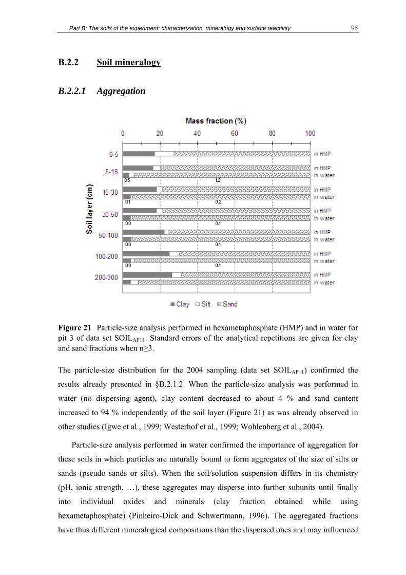
Part B: The soils of the experiment: characterization, mineralogy and surface reactivity 95
B.2.2 Soil mineralogy
B.2.2.1 Aggregation
Figure 21 Particle-size analysis performed in hexametaphosphate (HMP) and in water for pit 3 of data set SOILAP11. Standard errors of the analytical repetitions are given for clay and sand fractions when n≥3.
The particle-size distribution for the 2004 sampling (data set SOILAP11) confirmed the
results already presented in § B.2.1.2. When the particle-size analysis was performed in
water (no dispersing agent), clay content decreased to about 4 % and sand content
increased to 94 % independently of the soil layer ( Figure 21) as was already observed in
other studies (Igwe et al., 1999; Westerhof et al., 1999; Wohlenberg et al., 2004).
Particle-size analysis performed in water confirmed the importance of aggregation for
these soils in which particles are naturally bound to form aggregates of the size of silts or
sands (pseudo sands or silts). When the soil/solution suspension differs in its chemistry
(pH, ionic strength, …), these aggregates may disperse into further subunits until finally
into individual oxides and minerals (clay fraction obtained while using
hexametaphosphate) (Pinheiro-Dick and Schwertmann, 1996). The aggregated fractions
have thus different mineralogical compositions than the dispersed ones and may influenced

Part B: The soils of the experiment: characterization, mineralogy and surface reactivity 96
mineralogical studies. Here, we chose to disperse as much aggregates as possible in order
to analyze all the mineralogical clays of the soil matrix even if those clays were hidden
inside the aggregates.
B.2.2.2 Total chemical composition of bulk soil

97
Table 15 Mass proportion of total elements, amorphous (Ox) b and free (DCB) c Al and Fe contents in bulk soil for data sets SOILAP11 and SOIL15m. Standard errors for n≥3 are given in italic.
Soil layer N C SiO2 Fe2O3 Al2O3 MnO MgO CaO Na2O K2O TiO2 P2O5 LIa Fe2O3 Oxb Fe2O3 DCBc Al2O3 Ox Al2O3 DCB Alsubsd
cm % mol mol-1
Data set SOILAP11
0-5 0.18 0.05 3.20 1.03 81.62 1.43 3.29 0.11 5.16 0.31 0.02 0.00 0.04 0.00 0.80 0.02 0.04 0.01 8.69 1.99 0.12 0.01 2.67 0.08 0.21 0.03 0.88 0.01 0.29 0.01
5-15 0.06 0.00 0.79 0.01 84.35 0.05 3.70 0.12 6.02 0.31 0.02 0.00 0.03 0.00 0.94 0.05 0.04 0.00 4.69 0.09 0.11 0.00 2.58 0.02 0.16 0.00 0.78 0.01 0.28 0.00
15-30 0.05 0.00 0.68 0.04 83.81 0.71 3.72 0.12 6.08 0.34 0.03 0.00 0.03 0.00 0.93 0.02 0.04 0.00 4.55 0.18 0.10 0.00 2.63 0.02 0.15 0.01 0.77 0.02 0.28 0.00
30-50 0.04 0.00 0.55 0.02 83.07 0.43 3.87 0.07 6.41 0.17 0.03 0.00 0.03 0.00 1.00 0.01 0.03 0.00 4.58 0.09 0.09 0.00 2.99 0.22 0.14 0.00 0.86 0.07 0.28 0.00
50-100 0.03 0.00 0.47 0.01 81.71 0.66 4.49 0.10 7.79 0.19 0.03 0.00 0.03 0.00 1.16 0.03 0.04 0.00 4.95 0.12 0.08 0.00 3.59 0.07 0.16 0.00 1.04 0.02 0.28 0.00
200-300 0.02 0.00 0.22 0.01 79.04 1.05 4.95 0.19 8.62 0.40 0.04 0.00 0.04 0.00
<0.0
2
<0.0
7
<0.0
5
1.32 0.06 0.04 0.00 4.84 0.16 0.05 0.00 3.48 0.17 0.14 0.00 0.85 0.04 0.25 0.00
Data set SOIL15m
500 0.01 0.17 79.33 5.16 9.13 0.04 0.04 1.37 0.03 4.73 0.06 3.57 0.12 0.57 0.17 700 0.02 0.27 79.80 4.93 8.70 0.04 0.03 1.27 0.04 4.84 0.06 3.69 0.11 0.48 0.14 900 0.01 0.12 81.13 4.70 8.28 0.04 0.04 1.24 0.03 3.99 0.05 3.90 0.08 0.30 0.08
1100 0.01 0.12 84.29 3.86 6.26 0.04 0.03 1.17 0.03 3.18 3.06 0.26 1300 0.01 0.07 80.15 6.43 7.15 0.06 0.09 1.72 0.04 3.87 0.07 6.86 0.07 0.28 0.05 1500 0.00 0.04 82.41 5.89 5.15 0.10 0.10
<0.0
2
<0.0
7
<0.0
5
2.17 0.06 2.70 0.07 3.61 0.04 0.12 0.03
a LI = Loss on Ignition 110-1000°C; b Tamm, 1922 ; c Mehra & Jackson, 1960 ; d ( ) ( )
DCB Ox
DCB Ox DCB Ox
subs
Al AlAl
Al Al Fe Fe
−=
− + − where AlDCB, AlOx, FeDCB, FeOx are expressed in mole.

Part B: The soils of the experiment: characterization, mineralogy and surface reactivity 98
Total analysis of the bulk soil showed that it was constituted of about 80 % of SiO2, from 5
to 10 % of Al2O3, from 3 to 6.5 % of Fe2O3 and from 0.8 to 2 % of TiO2. MnO, MgO, K2O
and P2O5 total contents were < 0.05 %, CaO content was < 0.02 % and Na2O content <
0.07 %. The spatial variability for a given soil layer was low with standard errors < 0.7 %
for all the elements but SiO2, and < 2.5 % for SiO2 ( Table 15). The bulk soil composition
was homogeneous down to a depth of 15 m with a slight increase of Fe2O3, MnO, MgO
and TiO2 below a depth of 12 m.
Table 16 Pearson correlation coefficients between (i) total Al2O3, Fe2O3 and TiO2 and clay contents, and (ii) total SiO2 and sand contents calculated for data set SOILAP11, all soil layers taken altogether. Intercept and slope of the corresponding linear regressions are given for Fe2O3 and SiO2. All slopes and intercepts were significantly different from zero at P < 0.05.
Fe2O3 (%) Al2O3 (%) TiO2 (%) Clay (%) SiO2 (%) Fe2O3 (%) 1 Al2O3 (%) 0.997 1 (Fe2O3=0.885+0.467 Al2O3) TiO2 (%) 0.989 0.982 1 (Fe2O3=0.651+3.269 TiO2) Clay (%) 0.951 0.950 0.947 1 (Fe2O3=0.990+0.149 Clay) Sand (%) 0.919 (SiO2= 42.141+0.534 Sand)
Number of observations = 18.
The analysis of correlations showed that the SiO2 contents were highly correlated to
the sand contents, and Fe2O3, Al2O3, and TiO2 to the clay contents ( Table 16). The
corresponding linear regressions are easy tools to estimate total Fe, Al, Ti and Si contents
for this soil type from simple clay and sand content measurements.
Total analysis performed on the soil fractions confirmed these correlations showing
more silica (> 97 % of SiO2) in the sand fraction than in the silt and clay fractions, and
more Al, Fe and Ti in the clay fraction than in the sand and silt fractions (about a third of
the clay fraction was made of Al2O3, about 15 % of Fe2O3 and about 2.7 % of TiO2)
( ANNEX 3).
The chemical compositions of the bulk soil and of the soil fractions are in good
agreement with the literature (Alves and Lavorenti, 2004; Marques et al., 2004).

Part B: The soils of the experiment: characterization, mineralogy and surface reactivity 99
B.2.2.3 Identification of the minerals
Sand
Clay
d=0.
426
Qua
rtz
d=0.
334
Qua
rtz
d=0.
246
Qua
rtz
d=0.
228
Qua
rtz
d=0.
213
Qua
rtz
d=0.
720
kao
linite
d=1.
431
d=0.
484
gib
bsite
d=0.
358
kao
linite
5-15 cm
Block 3
Sand
Clay
d=0.
426
Qua
rtz
d=0.
334
Qua
rtz
d=0.
246
Qua
rtz
d=0.
228
Qua
rtz
d=0.
213
Qua
rtz
d=0.
720
kao
linite
d=1.
431
d=0.
484
gib
bsite
d=0.
358
kao
linite
5-15 cm
Block 3
Figure 22 Mineralogy of the clay and sand fractions: XR diffractograms performed on oriented deposit of the clay fraction Mg2+ saturated and on raw powder of the sand fraction for block 3, layer 5-15 cm of data set SOILAP11. The main peaks are given in nm together with the mineral they identify.
X-rays performed on soil fractions confirmed that the sand fraction was almost only made
of quartz and that the clay fraction was free of quartz (at a 5 % theoretical detection
threshold for X-ray analysis) ( Figure 22). The silt fraction presented intermediary features
between sands and clays, but as it represented less than 5% of the particle-size distribution,
less attention was put on this fraction.

Part B: The soils of the experiment: characterization, mineralogy and surface reactivity 100
200-300 cm
0-5 cm
d=1.
431
d=0.
358
kao
linite
d=0.
437
gib
bsite
d=0.
413
goe
thite
d=0.
485
gib
bsite
Clay fraction
Block 3
d=0.
720
kao
linite
d=0.
369
he
mat
ite
d=0.
269
hem
atite
+ go
ehtit
e
d=0.
252
hem
atite
d=0.
238
gib
bsite
200-300 cm
0-5 cm
d=1.
431
d=0.
358
kao
linite
d=0.
437
gib
bsite
d=0.
413
goe
thite
d=0.
485
gib
bsite
Clay fraction
Block 3
d=0.
720
kao
linite
d=0.
369
he
mat
ite
d=0.
269
hem
atite
+ go
ehtit
e
d=0.
252
hem
atite
d=0.
238
gib
bsite
Figure 23 Homogeneity with depth of the mineralogy of the clay fraction: RX diffractograms performed on raw powder of the clay fraction Mg2+ saturated for block 3 of data set SOILAP11, layers 0-5 cm and 200-300 cm. The main peaks are given in nm together with the mineral they identify.
The X-ray analysis performed on the oriented clay deposits and on raw powder of the
clay fraction showed the characteristics reflections of kaolinite (0.72 and 0.357 nm),
gibbsite (0.485 and 0.437 nm, reflexions at 0.431 and 0.238 nm), goethite (0.418, 0.269
nm) and hematite (0.270 and 0.252 nm) (Dixon and Weed, 1989). RX analysis showed that
the clay mineralogy was highly homogeneous whatever the depth sampled. A slight
increase in gibbsite and hematite contents in deeper soil layers is suggested ( Figure 23).

Part B: The soils of the experiment: characterization, mineralogy and surface reactivity 101
Block 1
0-5 cm
Clay fraction
d=0.
720
kaol
inite
d=1.
431
d=0.
484
gib
bsite
d=0.
358
kao
linite
d=0.
437
gib
bsite
d=0.
413
goe
thite
Block 2
Block 3
Block 4
Block 1
0-5 cm
Clay fraction
d=0.
720
kaol
inite
d=1.
431
d=0.
484
gib
bsite
d=0.
358
kao
linite
d=0.
437
gib
bsite
d=0.
413
goe
thite
Block 2
Block 3
Block 4
Figure 24 Spatial homogeneity of the mineralogy of the clay fraction: RX diffractograms performed on oriented deposit of the clay fraction Mg2+ saturated for all blocks of data set SOILAP11, layer 0-5 cm. The main peaks are given in nm together with the mineral they identify.
RX spectra showed a great homogeneity according to blocks. Spectra are given for the
clay fraction at depth 0-5 cm for which the maximum heterogeneity was expected ( Figure
24).

Part B: The soils of the experiment: characterization, mineralogy and surface reactivity 102
Mg2+ saturated
d=1.
431
HIM
d=0.
718
kaol
inite
Mg2+ saturatedEG treatment
DCB+Tricitrate treatmentsK+ saturated
Mg2+ saturated550°C heating
Clay fraction
Block 3
5-15 cm
Mg2+ saturated
d=1.
431
HIM
d=0.
718
kaol
inite
Mg2+ saturatedEG treatment
DCB+Tricitrate treatmentsK+ saturated
Mg2+ saturated550°C heating
Clay fraction
Block 3
5-15 cm
Figure 25 Identification of the peak at 1.431 nm: influence of treatments (Mg2+ saturation, ethylene glycol (EG) treatment, DCB followed by tricitrate extractions and saturation by K+, heating at 550°C) on RX diffractograms performed on oriented deposits of the clay fraction for layer 5-15 cm block 3 of data set SOILAP11.
A peak at 1.4 nm indicated the presence of a 2:1 phyllosilicate visible for bulk soil
samples as well as for oriented clay deposits. Its location changed neither after treatment
with ethylene glycol nor after DCB+Tamura treatments and K+ saturation, but the peak
disappeared after heating at 550°C together with the kaolinite peaks, as classically
observed (Bish and Duffy, 1990; Dejou et al., 1977). No peak appeared at 1.0 nm after
heating at 550°C ( Figure 25).

Part B: The soils of the experiment: characterization, mineralogy and surface reactivity 103
According to Table 9, the X-ray patterns of the 2:1 mineral corresponded to a
hydroxylated interlayered mineral present in small amounts since it was not always visible
on X-ray charts and since no peak appeared after heating at 1 nm (below the detection
threshold of 5%). Such minerals have been observed in highly weathered tropical soils
(Bryant and Macedo, 1990; Fontes and Weed, 1991; Kampf and Schwertmann, 1983;
Olmos I. L et al., 1993) and their occurrence in tropical soils is not well understood.
Hydroxy-Al interlayered smectite and vermiculite are thought to occur as either weathering
products derived from chlorite weathering or more commonly from the deposition of
hydroxy-Al polymeric components within the interlayer spaces of these expansible or
limited expansible layer silicates (Barnhisel and Bertsch, 1989). It has been suggested that
moderately acidic conditions, low organic matter content, oxidizing conditions, and
frequent wetting and drying cycles are optimal environmental conditions for pedogenic
hydroxy-Al interlayer formation. Other authors have also suggested that the interlayer
component was a kaolin mineral and not a hydroxy-Al polymeric material. They proposed
that the structure of the intergradient vermiculite-kaolin mineral consisted of vermiculite
and vermiculite that had been transformed to double kaolin layers (Wada and Kakuto,
1983). This type of structure may explain the disappearance of all peaks after heating at
550°C without any newly formed peak at 10 nm, since kaolinite mineral structure is lost at
such a temperature.
B.2.2.4 Fe and Al specific extractions
Al2O3 extracted by the oxalate treatment (Tamm) was about 0.15 % of the bulk soil
mass. It was a little more in the 0-5 cm layer where it reached 0.21 %. DCB treatment
(Mehra & Jackson) extracted about 0.8 % of aluminium (expressed in Al2O3) whatever the
soil layer. Beyond a depth of 3 m, aluminium extracted by both treatments decreased
gradually down to a depth of 15 m where it reached values < 0.04 % for the oxalate
extraction and < 0.12 % for the DCB extraction ( Table 15).
Iron extracted by the oxalate treatment decreased gradually with depth from 0.12 % of
iron expressed in Fe2O3 in the 0-5 cm layer, to 0.05 % beyond a depth of 3 m. DCB
treatment extracted about 2.6 % of iron expressed in Fe2O3 down to a depth of 50 cm,
about 3.5 % beyond a depth of 50 cm, and about 7 % at depths 12, 13 and 14 m ( Table 15).
The oxalate treatment extracted less than 4 % of total iron and less than 5 % of total
aluminium. DCB treatment extracted about 75 % of total iron and less than 15 % of total

Part B: The soils of the experiment: characterization, mineralogy and surface reactivity 104
aluminium. Most standard deviations were quasi systematically < 10 % of the measured
value.
The amounts of iron and aluminium extracted for the same soil type are generally
larger in other studies (Alves and Lavorenti, 2004; Bryant and Macedo, 1990; Kampf and
Schwertmann, 1983; Neufeldt et al., 1999; Olmos I. L et al., 1993). A one-hour single
extraction was performed in the present work whereas other studies report that longer
contact times or successive extractions are necessary to extract all free Al and Fe in these
soils particularly rich in oxides (Fontes and Weed, 1991; Loeppert and Inskeep, 1996).
Figure 26 Al2O3 extracted (%) by different analytical methods (oxalate, DCB and tricitrate) from the clay fraction of pit 3 of data set SOILAP11. Al2O3 from gibbsite and kaolinite estimated from § B.2.2.5 are also represented.

Part B: The soils of the experiment: characterization, mineralogy and surface reactivity 105
These extractions were also performed on soil fractions. The results for the clay
fraction are presented in figure Figure 26 for aluminium. Complete results are given in
ANNEX 3 but will not be discussed here. Oxalate extracted less than 0.9 % of aluminium
(expressed in Al2O3), DCB treatment extracted less than 3 % of Al2O3, and tricitrate
treatment (Tamura) about 1.7 % of Al2O3. DCB treatment immediately followed by
tricitrate treatment extracted about 4.7 % of aluminium which equals the sum of aluminium
extracted independently by DCB treatment and tricitrate treatment.
B.2.2.5 Quantitative estimation of soil mineralogy
0.00 0.20 0.40 0.60 0.80 1.00
0-5
5-15
15-30
50-100
200-300
Soil
laye
r (cm
)
Mass fraction
QuartzKaoliniteGibbsiteHematiteGoethiteTiO2Organic matterOther
Figure 27 Estimated mineralogical composition of the bulk soil calculated from § B.1.2.6.4 for pit 3 of data set SOILAP11.
The clay fraction contained about 35 % of Al2O3. About 24 % were attributed to kaolinite
and 11% to gibbsite (data not shown). The corresponding bulk soil composition was of
about 70 to 80 % of quartz, 10 to 15 % of kaolinite, 0.5 to 4.5 % of gibbsite, 0 to 3.7 % of
hematite and 1.3 to 3.5 % of goethite. The 0-5 cm layer was slightly depleted in quartz and
gibbsite, but enriched in organic matter ( Figure 27) in comparison to deeper layers. The
sum of all estimated minerals reconstituted more than 98 % and less than 102 % of the
total soil mass. It is reminded that Figure 27 represents the total composition of the soils of
pit 3 which may differ slightly from the average bulk soil composition, particularly for
organic matter in the 0-5 cm layer where the heterogeneity is greatest.

Part B: The soils of the experiment: characterization, mineralogy and surface reactivity 106
The estimated kaolinite and gibbsite compositions were checked thanks to TGA
results. The weight losses recorded by TGA or estimated from the previous calculation are
given for the clay fraction in Table 17. It confirmed the order of magnitude of the
estimated kaolinite compositions. Results for gibbsite and goethite are less consistent but
the TGA results for these two minerals are less reliable since they interfere with each other
in the range 220-320°C (Bish and Duffy, 1990; Dejou et al., 1977).
Table 17 Weight losses (%) measured by thermogravimetry compared to weight losses from the normative calculation of the clay fraction for pit 3 of data set SOILAP11.
Weight losses (%) Simulated (normative calculation) Thermogravimetry Soil layer (cm) Kaolinite Goethite+hematite Kaolinite Goethite+hematite 0-5 9.02 5.55 8.17 4.24 5-15 8.42 6.81 7.22 4.19 15-30 8.38 6.51 7.60 4.17 50-100 8.31 6.11 7.13 4.58 200-300 8.10 6.45 7.42 4.79
It is rather difficult to quantitatively differentiate goethite from hematite. Classically,
such determinations are performed after isolating the oxide fractions by selective
dissolutions of kaolinite and gibbsite by NaOH (Balwant and Gilkes, 1991; Cornell and
Schwertmann, 2003), then by comparing the relative intensity of some specific reflections
of the RX spectra. Goethite and hematite have also been quantified from the ratio of citrate
extractable Fe and Al compared to DCB extractable Fe and Al at 20°C (Cornell and
Schwertmann, 2003). Such analyses were not considered essential within the scope of this
study since neither hematite nor goethite is likely to release nutrients by weathering.
Goethite versus hematite ratios were taken from the literature on yellowing as already
mentioned, but since they were not calculated from direct measurements, goethite and
hematite contents must be handled cautiously and regarded much as an order of magnitude.
In the calculation, all the aluminium which was not attributed to kaolinite was
attributed to gibbsite. However, there may be other minerals containing Al which were not
taken into account (in particular phyllosilicate at 1.4 nm). Thermogravimetric analysis
seemed to confirm the overestimation of gibbsite. Actually, Al may substitute Fe in
goethite and hematite. For our soil types, rates of substitution < 10 % (mole) for hematite
and between 15 and 25 % (mole) for goethite are frequently reported (Anand and Gilkes,
1987; Bryant and Macedo, 1990; Fontes and Weed, 1991). This substitution was not

Part B: The soils of the experiment: characterization, mineralogy and surface reactivity 107
considered in the calculations since the contents of hematite versus goethite were
uncertain, but it can be estimated from the DCB and Tamura extractions performed on the
clay fraction. For those samples, the aluminium extracted by the Tamura reactant seemed
to be part of a mineral fraction different from that extracted by the DCB reactant since the
Al extracted by the DCB treatment followed by the Tamura treatment equaled the sum of
each extraction performed independently. Since the DCB extraction is reported to extract
goethite + hematite oxides, one can suppose that the DCB extraction extracted the Al
substituted in goethite and hematite. The ratio AlDCB/(AlDCB+FeDCB) was between 0.25 and
0.30 which actually corresponded to the substitution ratios given by the literature for
goethite. Introducing Al-substitution in the calculations led to gibbsite contents for the clay
fraction of 12 % which is close to the gibbsite contents calculated from the TGA analysis.
As titanium content was < 5% in bulk soil and in soil fractions, it was impossible to
determine its mineralogical nature by X-ray diffraction. It was thus kept in calculations as
TiO2 (rutile) but it may exist in association with other elements in soils, especially iron to
form ilmenite FeTiO3. The occurrence of this mineral is frequently reported for tropical
ferralsols (Cornell and Schwertmann, 2003; Nzila, 2001; Olmos I. L et al., 1993) and is
generally found in association with magnetite Fe3O4 (Dixon and Weed, 1989; Pinheiro-
Dick and Schwertmann, 1996). A black powder with magnetic properties was
systematically found in all soil fractions. This powder was isolated and unsuccessfully
analyzed by X-ray diffractometry but was very likely magnetite. The presence of ilmenite
and magnetite may slightly decrease the calculated contents of hematite and goethite.
The resulting mineralogical composition for bulk soil and clay fraction was in good
agreement with the literature (Costa et al., 2004; Fontes and Weed, 1991).
B.2.2.6 Conclusion: weathering potential and expected soil surface
reactivity
The mineralogical composition obtained is typical of Dystrophic Red-Yellow Latosols
which contains large quantities of well crystallized iron and aluminium oxides, few
amorphous aluminium and iron, and mainly kaolinite in its clay fraction. The mineralogy
of the bulk soil was highly homogeneous. All minerals were common to all soil layers and
blocks sampled but were present in different amounts depending mainly on the soil layer.
A slight change in the mineralogy is suggested below a depth of 12 m but further
mineralogical analysis, including X-ray diffractions of the clay fraction would be necessary

Part B: The soils of the experiment: characterization, mineralogy and surface reactivity 108
to confirm this hypothesis. It was not regarded as a priority within the scope of this study.
The identified 2:1 phyllosilicate is very stable since it remained unaffected by DCB or
Tamura treatments and only lost its mineral structure after heating at 550°C. Together with
total analyses which indicated total bulk soil contents of Mg, K, Na and Ca < 0.07 %, this
meant that no significant amount of these elements may be released in soil solution by
weathering.
As for surface reactivity, the mineralogical composition indicates that a general
behavior of variable charge soil may be expected. Amorphous iron and aluminium are not
present in large quantities so that the anion exchange capacity may be limited at soil pH
and mainly hold by hematite, goethite and gibbsite. According to Table 8, kaolinite is
expected to be little charged at soil pH and the CEC must be mainly carried by the organic
matter. The HIM may exhibit a large capacity to retain cations since the permanent charge
of the vermiculite is about 170 cmolc kg-1. Even present in little quantity, such a mineral
may greatly influence the CEC. Yet, the permanent charge of HIM is partly compensated
by the interlayered aluminium so that the resulting charge is reduced (Dixon and Weed,
1989). The CEC of the clay fraction measured was about 6 cmolc kg-1 ( Table 18) which is
approximately the CEC of kaolinite at pH 5. Even if the HIM mineral participates to this
CEC, the permanent charge of such a mineral seems to be limited.
Table 18 Cation exchange capacity of the clay fraction measured by Sr saturation in cmol/kg. Standard errors are given in brackets for n≥3.
Depth CEC clay fractioncm cmolc kg-1
0-5 8.10 (1.045) 5-15 6.16 15-30 5.69 30-50 50-100 5.50 100-200 200-300 6.49

Part B: The soils of the experiment: characterization, mineralogy and surface reactivity 109
B.2.3 Surface reactivity
B.2.3.1 CEC & pH: complement to § B.2.1
Table 19 pH in water and in KCl 1 mol L-1, effective cation exchange capacity (CEC in cmolc kg-1) and saturation in alkaline earth cations (Sat in cmolc kg-1) measured every meter down to a depth of 15 m for data set SOIL15m (n=1).
Depth pH H2O pH KCl Sat CEC Sat/Tcm - - cmolc kg-1 %
100 5.9 4.5 0.58 1200 6.0 5.4 0.25 1300 5.9 5.3 0.08 8400 6.1 5.2 0.02 42500 5.9 5.6 0.06 9600 6.1 5.1 0.19 3700 6.0 5.5 0.26 1800 6.0 5.7 0.32 4900 5.7 4.7 0.26 11000 6.0 4.9 0.52 11100 5.5 5.0
<0.01
0.40 11200 5.1 4.0 0.02 1.33 11300 5.1 4.3 0.01 1.55 11400 4.8 4.1 1.87 01500 4.8 4.2
<0.01 2.09 0
No inversion between pH in water and in KCl occurred down to a depth of 15 m which
meant that CEC always prevailed over AEC even in very deep soil layers. The change in
soil mineralogy suggested in § B.2.2.2 seems to be confirmed by the CEC values which
increased below a depth of 12 m to more than 1.5 cmolc kg-1 ( Table 19). Nevertheless, the
saturation in basic cations remained very low with almost 100% of the cation exchange
capacity saturated by aluminium. These results suggest that the soil matrix holds a large
capacity to retain cations and anions which might be leached below a depth of 3 m,
especially through the large volume of exchanger available (soil profile deeper than 15
m…).
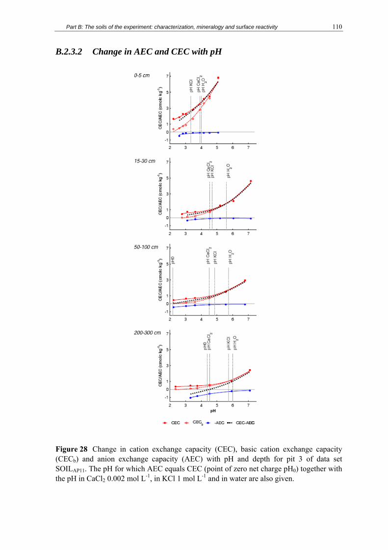
Part B: The soils of the experiment: characterization, mineralogy and surface reactivity 110
B.2.3.2 Change in AEC and CEC with pH
Figure 28 Change in cation exchange capacity (CEC), basic cation exchange capacity (CECb) and anion exchange capacity (AEC) with pH and depth for pit 3 of data set SOILAP11. The pH for which AEC equals CEC (point of zero net charge pH0) together with the pH in CaCl2 0.002 mol L-1, in KCl 1 mol L-1 and in water are also given.

Part B: The soils of the experiment: characterization, mineralogy and surface reactivity 111
As expected, the AEC and CEC varied with the pH of the contact solution ( Figure 28):
CEC increased and AEC decreased with pH. The CEC was almost constant below pH=4.5
and was saturated with aluminium. The basic cation exchange capacity (CECb) was null at
about pH 2.5 which is the point of zero charge of quartz. The upper soil layer (0-5 cm)
exhibited a greater CEC due to its high organic matter content. The AEC was null at pH 7-
8 which is the point of zero charge of iron and aluminium oxides. AEC was greatest for the
200-300 cm layer.
The pH for which AEC equaled CEC (point of zero net charge pH0) increased with
depth. It was < 2 for the 0-5 cm layer, about 2 down to a depth of 1 m, 3.2 for the 100-200
cm layer and 4.4 for the 200-300 cm layer where it equaled soil pH. The pH in CaCl2 0.002
mol L-1 was 4.5 for all soil layers except for the 0-5 cm layer for which it was 3.9 ( Figure
28 and Table 20).
CEC and AEC changes with pH as well as points of zero charge are in good agreement
with the literature (Chorover and Sposito, 1995; Curtin and Syers, 1990a; Marcano-
Martinez and McBride, 1989; Soares et al., 2005; Van Raij and Peech, 1972; Van Ranst et
al., 1998).
Table 20 Cation exchange capacity (CEC), basic cation exchange capacity (CECb), and anion exchange capacity at soil pH measured in CaCl2 0.002 mol L-1 (no HCl or CaOH2 addition) for pit 3 of data set SOILAP11. The pH for which AEC equals CEC (pH0) together with the pH in KCl 1 mol L-1 and in water are also given.
pH Layer CECb CEC AEC pH0
CaCl2 0.002 mol L-1
KCl 1 mol L-1 water
cm cmolc kg-1 - 0-5 2.78 3.50 0.10 - 3.9 3.3 4.0 5-15 0.85 1.21 0.08 1.7 4.5 4.5 5.6 15-30 0.70 0.89 0.09 2.0 4.5 4.7 5.6 30-50 0.75 0.97 0.13 2.1 4.5 4.7 5.0 50-100 0.66 0.87 0.14 2.2 4.5 4.9 5.7 100-200 0.56 0.71 0.30 3.2 4.5 4.9 5.8 200-300 0.51 0.58 0.53 4.4 4.5 5.7 6.0

Part B: The soils of the experiment: characterization, mineralogy and surface reactivity 112
B.2.3.3 Specific adsorption of nitrate, sulphate and phosphate
0 25 50-50
20
40
60N
ad
sorb
ed (
mg
/100
g)
0 50 100-50
20
40
60
S a
dso
rbed
(m
g/1
00g
)
0 40 80-50
20
40
60
P a
dso
rbed
(m
g/1
00g
)
0 25 50-50
20
40
60
N concentration (mg L-1)
N a
dso
rbed
(m
g/1
00g
)
0 50 100-50
20
40
60
S concentration (mg L-1)
S a
dso
rbed
(m
g/1
00g
)
0 40 80-50
20
40
60
P concentration (mg L-1)
P a
dso
rbed
(m
g/1
00g
)
0 5 10 15 20 25 30 35 40-1
0
1
Measured data Langmuir isotherm Freundlich isotherm Zone AEC
Figure 29 Isotherms of adsorption measured for the 0-5 cm layer (A) and the 200-300 cm layer (B) for nitrate, sulphate and phosphate. The Langmuir and Freundlich equations fitted on experimental data are represented. The grey zone on the graphics corresponds to the equivalent AEC (values of Table 20) for N-NO3
-, S-SO42-, and H-H2PO4
-.
The adsorption isotherms measured at pH 4 and for a ionic strength of 100 mmol L-1
(KCl as indifferent electrolyte) failed to show any specific adsorption of nitrates, but
revealed the specific adsorption of sulphate for the 200-300 cm layer, and the increasing
adsorption of phosphate with soil depth ( Figure 29). The experimental reproducibility was
good with standard errors < 1 mg/100g for qads and < 1 mg L-1 for csolution (n=3) except for
the greatest concentration for which they were < 2.
The Langmuir equation fitted well the data ( Table 21). The maximum adsorption is
given by maxadsq of the Langmuir equations (equation (26)) and was of 22 mg S / 100 g for
the 200-300 cm layer, 37 mg P / 100 g for the 0-5 layer and 46 mg P / 100 g for the 200-
300 cm layer. Such maximum values of adsorption are in good agreement with the
literature for our soil type (Agbenin and Tiessen, 1994; Alves and Lavorenti, 2004; Couto
et al., 1979; Gillman, 1984; Marcano-Martinez and McBride, 1989).
A
B

Part B: The soils of the experiment: characterization, mineralogy and surface reactivity 113
Table 21 Langmuir and Freundlich parameters fitted on the experimental data for the 0-5 cm layer (P) and the 200-300 cm layer (S and P). The sum of square errors (SSE) and the number of observations (n) are given.
Langmuir 1 Freundlich 2 Layer Element max
adsq K SSE n kf nf SSE n cm mg/100g L mol-1
0-5 P 37 10 67 21 5.8 0.4 82 21
200-300 S 22 11 36 21 3.6 0.4 67
P 46 1 450 21 17.9 0.3 671
1 max
1ads
solutionads
solution
Kcq qKc
=+
eq (26); 2 1/ f
ads
nf solutionq k c= eq (27), where qads is the quantity of N, S or P
adsorbed on the soil surface (mg/100g) and csolution is the concentration of N, S or P in the contact solution
(mg L-1)
B.2.3.4 Conclusion
The changes in CEC and AEC with the pH of the contact solution confirmed that the
variable charges dominate in the soils of the experiment. Graphics are compatible with a
small permanent charge of about -0.5 cmolc kg-1 but the experimental measurement of the
permanent charge as explained by Chorover and Sposito (1995) or Gillman and Sumner
(1987) would be necessary to rule on this point.
The upper soil layer (0-5 cm) is dominated by the CEC of the organic matter whereas
AEC increased in deeper layers (200-300 cm) together with Fe and Al oxide contents of
the clay fraction. The CEC and the AEC remained small at soil pH with mean values < ± 1
cmolc kg-1. Cation retention may thus occur mainly in upper soil layers whereas anion
retention may mainly occur in deeper soil layers below a depth of 50 cm. A change in pH
would lead to a significant increase in CEC above pH 6, and a significant increase in AEC
below pH 4 mainly in deep soil layers (below a depth of 50 cm).
Specific adsorption may occur for phosphate whatever the soil layer and for sulphate
for soil layers which are not greatly influenced by organic matter. Such adsorptions were
recorded at pH 4 but would change under different pH conditions, soil solution status
(ionic strength, composition) and soil surface status (aggregation, previously adsorbed
species).

Part B: The soils of the experiment: characterization, mineralogy and surface reactivity 114
B.3 GENERAL CONCLUSIONS
B.3.1 On soil general features
The soils of the experiment correspond to Dystrophic Red-Yellow Latosols and are
characterized by (i) yellow/red hues, (ii) an upper soil horizon influenced by OM and a
horizon below a depth of 50-70 cm with an increase of 8 % in the clay content compared to
the upper soil layers, and (iii) very low CEC and organic matter content (CEC < 1 cmolc
kg-1, C < 0.6 % and N < 0.05 % below a depth of 15 cm). The soil surface behaviour is of a
variable charge system (permanent charge < 0.5 cmolc kg-1) for which CEC prevails in the
upper soil layers and equals AEC in deep soil layers. Specific adsorptions of S and P occur.
B.3.2 On soil spatial heterogeneity
Most of the variability is localized in the upper soil layer (0-5 cm) and results from organic
matter heterogeneities. In contrary, physical and chemical properties are highly
homogeneous in deep soil layers. The variability among the sampled plots grouped by
treatment or by block is of the same order of magnitude than the variability inside each
plot, where a slight effect of the distance to the nearest trees was observed. This means that
the changes which may be observed in the studied variables during the fertilization
experiment may be attributed to the treatments established provided that the soils are
sampled continuously from the stump to the inter-row.
B.3.3 On mineral weathering
The soils contain large quantities of quartz and well crystallized iron and aluminium
oxides, few amorphous aluminium and iron, and mainly kaolinite in its clay fraction. The
identified 2:1 phyllosilicate is very stable since it remained unaffected by DCB or Tamura
treatments and only lost its mineral structure after heating at 550°C. Together with total
analyses which indicated total bulk soil contents of Mg, K, Na and Ca < 0.07 %, this
means that no significant amount of these elements may be released in soil solution by
weathering. On the other hand, Al, Fe and Si may be released by the weathering of
kaolinite and of more or less crystallized oxides.

Part B: The soils of the experiment: characterization, mineralogy and surface reactivity 115
B.3.4 On the expected soil response to the applied fertilizations
Table 22 Estimation of the capacity of the soil (in kg ha-1) to retain cation or anion by non specific adsorption (CEC and AEC) or specific adsorption. For each element, the capacity is calculated for each soil layer from the bulk density of Table 11 and the CEC or AEC of Table 20 fully saturated with the studied element. The charge attributed to each element is +1 for Na, K and N-NH4, +2 for Ca and Mg, +3 for Al, -1 for N-NO3, Cl and P-H2PO4, and -2 for S-SO4. Specific adsorptions are calculated from Table 21. n.d.=not determined.
CEC AEC Specific adsorption Na K Ca Mg Al N-NH4 N-NO3 Cl S-SO4 P-PO4 S-SO4 P-PO4
kg ha-1
0-5 cm 511 869 446 270 200 311 9 23 10 20 0 2325-15 cm 378 642 329 200 148 230 15 38 17 33 n.d. n.d.
15-30 cm 443 753 386 234 173 270 27 69 31 61 n.d. n.d.30-50 cm 628 1067 547 332 246 382 53 134 61 117 n.d. n.d.
50-100 cm 1394 2371 1215 737 545 849 132 334 151 292 n.d. n.d.100-200 cm 2270 3861 1979 1200 888 1382 578 1464 662 1279 n.d. n.d.200-300 cm 1852 3150 1614 979 725 1128 1031 2611 118 228 2996 6405
For cations, the fertilizers applied in treatments 1 and 3 brought about 400 kg ha-1 of
Ca, 224 kg ha-1 of Mg, 107 kg ha-1 of K and 5 kg ha-1 of Na. Table 22 indicates that if Ca
and Mg were preferentially adsorbed and if all the fertilizers were dissolved, the CEC of
the 0-5 cm and 5-15 cm would be necessary to retain the Ca and Mg issued from the
fertilizers. The other cations would then be leached down to 30 cm. As Al is preferentially
adsorbed on CEC for acidic soil pH and as the CEC is already saturated by more than 80 %
of aluminium, the negative sites effectively available for the adsorption of base cations
may be highly reduced, and it is likely that some cations may be leached in deeper soil
layers. If recalculating Table 22 from a reduced CEC (=20% of total measured CEC), the
entire profile down to a depth of 3 m would be necessary to retain the cations contained in
the fertilizers.
For anions, Cl is reported to be adsorbed preferentially over NO3 by non specific
adsorption. If all the Cl within the fertilizers was to be dissolved (95 kg ha-1), the 0-5 cm,
5-15 cm and 15-30 cm would be necessary to adsorb it on their AEC. Nitrate would be
leached in deeper horizons and all the soil layers down to 200 cm would be necessary to
retain the N-NO3 issued from the fertilizers (121 kg N ha-1 in T3 and 360 kg N ha-1 in T5)
by adsorption. The S-SO4 in fertilizers (141 kg ha-1 in T3 and 171 kg ha-1 in T5) may
compete for these adsorption sites but the specific adsorption capacity of deeper soil layers

Part B: The soils of the experiment: characterization, mineralogy and surface reactivity 116
(probably below a depth of 30 cm) would be sufficient to adsorb it. The specific adsorption
capacity of P in the 0-5 cm layer is sufficient to hold the P inputs by fertilization (35 kg ha-
1 in T1 and T3, and 138 kg ha-1 in T5) so that P may not appear much in soil solutions.
Of course, all the fertilizers may not dissolve entirely at once and the immobilization
in the soil organic matter and micro-organisms and in the vegetation biomass would
considerably reduce the release of nutrients in soil solution. Moreover, specific interactions
among nutrients such as Ca with SO4 and PO4 (as already mentioned in the introduction)
may modify substantially this simplistic scheme. The clear felling would also release
important quantities of N-NO3 in soil solution by mineralization of the forest floor and of
harvest residues, which may be adsorbed on AEC previously to the anions (in particular Cl
and NO3) brought by the fertilizers. Nitrogen may also be retained as N-NH4 on the CEC.
CEC and AEC may also change with soil solution chemistry and pH. The
mineralization of the soil organic matter after clear felling is expected to release protons in
soil solution and thus to lead to more acidic pH and thus to enhance AEC over CEC. The
fertilization on the other hand brought dolomitic limestone which may have the opposite
effect. Phosphate, if specifically adsorbed, may also lower the PZC and thus increase
cation retention. The adsorbed species may then reorganize slowly after the clear felling
and the fertilization episodes, by immobilization, diffusion and occlusion into the
aggregates and into minerals, desorption… While the time elapses, the soils may tend to
return to their initial pH close to their PZNC (which is the thermodynamically stable state)
if soil constituents have not been too much altered by the changes in pH and soil surface
status.
In conclusion, the leaching of monovalent cations is expected down to a depth of 3 m,
and of divalent cations down to 50-100 cm. P is expected to be quickly adsorbed in the
upper soil layer (0-5 cm) and to appear little in soil solutions, especially in ZTL (zero
tension lysimeter) which collects solutions in a narrow range of pressure heads. Sulphates
are expected to be leached deeper down to a depth of 30-50 cm where they may be
adsorbed on the soil surface. Cl may be adsorbed from the upper soil layer down to a depth
of 30-50 cm, and NO3 is expected to be leached down to 50-100 cm where it may be
adsorbed on soil surface. Specific interactions between Ca and SO4 or PO4 suggest that
these elements may appear concomitantly in soil solution.

Part B: The soils of the experiment: characterization, mineralogy and surface reactivity 117
B.3.5 On the methods used
Aggregation in our soil was highly dependant upon the soil solution chemisty. It would be
interesting to further investigate (i) which surfaces (type and quantity) are available for
adsorption depending on the soil aggregation status, and (ii) the nature of the organo-
mineral associations constituting the aggregates.
Regarding the mineralogical study, further analysis would be needed to identify and
quantify the oxides more precisely. Simple analyses which may be performed are for
example (i) X-ray diffractions performed on the oxide fraction after removal of the other
minerals (kaolinite), (ii) repeated extractions by dithionite-citrate-bicarbonate at 25°C
compared to extractions with citrate-bicarbonate at 25°C, (iii) MEB observations,
microprobe sampling and total analysis. Further analyses would also be needed to rule on
the nature of the phyllosilicate at 1.4 nm, such as MEB observations, microprobe sampling
and total analysis, progressive heating coupled to X-ray diffraction, …
Regarding the soil surface reactivity, adsorption isotherms were only performed at
pH=4 for a given ionic strength and two soil layers (0-5 and 200-300 cm). Isotherms would
be needed for the other soil layers, in particular for S which exhibited a broad gradient of
maximum specific adorption from the upper soil layer down to a depth of 3m. Moreover,
pH=4 corresponded to the lower values of pH observed in the experiment (soil pH and soil
solution pH), but one more modality such as pH=6 would be needed to assess the range of
variations of the S and P specific adsorptions within the range of variations of pH in the
fertilization experiment. The desorption dynamics together with the possible interactions
among other cations and anions would also need investigating.
Regarding the modelling of the soil/solution interactions, the calibration of the models
requires precise knowledge of the soil mineralogy and surface reactivity. It is thus
important to have reliable measurements of these characteristics for the studied soils within
the range of variations expected for the control parameters (ionic strength, pH, …).

Part B: The soils of the experiment: characterization, mineralogy and surface reactivity 118

119
PART C
WATER FLUXES


Part C : Water fluxes 121
INTRODUCTION
Soil water is a major component which integrates many physical, chemical and biological
phenomena within forest ecosystems. While computing input-output budget of nutrients
(Ranger and Turpault, 1999), precise knowledge of water fluxes in forest soils is needed to
assess nutrient losses by drainage. As it is quite difficult to quantitatively measure soil
water fluxes, modelling of water fluxes is classically used to compute soil water balance of
the ecosystem (Beier, 1998; Granier et al., 1999a; Hornbeck et al., 1997; Ranger and
Turpault, 1999; Ranger et al., 2002; Tsutsumi, 1969; Turpault et al., 1999; Williams,
1987). Nutrient balance will thus be highly dependant on the accuracy of such models
especially for forest soils for which the hydrodynamic structures are highly heterogeneous
(Fournier et al., 1994; Riha et al., 1986) and the collection of information (velocity,
porosity) from field experiments, is a crucial step for precise calibration and setting up of
deterministic flow or transport models (Ptak et al., 2004).
The water flow in soils is generally heterogeneous. As recalled by Dreuer et al. (2003),
the causes of preferential or bypass flow are related to hydraulic characteristics such as the
occurrence of macropores (Beven and Germann, 1982), dual or multimodal pore-size
distributions (Gerke and van Genuchten, 1993; Zurmühl and Durner, 1996), discontinuities
of texture (Kung, 1990) and the occurrence of biopores such as root channels (Bramley et
al., 2003; Parsons et al., 2004). Many of the manifestations of preferential flow and
transport have their genesis at the soil profile upper boundary (Clothier et al., 2008)
through heterogeneous water inputs at the soil upper boundary or differences in infiltration
resulting from heterogeneity of wettability of the soil surface. This is particularly true in
forest ecosystems for which incident rainfall may be spatially distributed through stemflow
and throughfall (Levia and Frost, 2003; Levia and Frost, 2006), and hydrophobic forest
floor such as the Eucalyptus one may infiltrate water heterogeneously (Greiffenhagen et
al., 2006; Laclau et al., 2004a).
Hydraulic properties of tropical ferralsols are reported to be highly homogeneous at a
macroscopic scale (> 1 m) but to show random-like variations at a microscopic scale
(Cichota et al., 2006). This heterogeneity is directly related to the microaggregated
structure of ferralsols already presented in part B (Balbino et al., 2004; Pochet et al., 2007;
Volland-Tuduri et al., 2004). The inter-aggregate porosity explains the high hydraulic

Part C : Water fluxes 122
conductivity at saturation classically recorded for this type of soil of about 1-50 10-5 m s-1
(Balbino et al., 2004; Elsenbeer et al., 1999; Paiva et al., 2000; Pochet et al., 2007). This
first type of porosity corresponds to pore diameters of 5 to 300 microns (pressure heads > -
6m) which are extremely permeable to water (Cambier and Prost, 1981; Cornell and
Schwertmann, 2003) and represent about half of total soil porosity (Balbino et al., 2002;
Cambier and Prost, 1981; Neufeldt et al., 1999). The diameter of the second pore class
associated to intra-aggregate porosity is about 20 nm (pressure head of about -1500m)
(Balbino et al., 2002; Cambier and Prost, 1981; Neufeldt et al., 1999) and results in a high
hydrodynamic dispersion (Cambier and Prost, 1981). Such pressure heads are hardly
recorded experimentally in the field and a single pore distribution may be tested as a first
modelling approach but a second class of porosity may be of crucial importance in terms of
chemical reactivity.
The soil water fluxes are also highly dependant upon the transpiration of on-site
vegetation and upon the evaporation of the upper soil layers. These two fluxes may take up
a large amount of water (sink term) from the soil profile. The transpiration of fast-growing
Eucalyptus trees is classically reported to be large (Almeida et al., 2007; Damman, 2001;
Laclau, 2001; Soares and Almeida, 2001; Whitehead and Beadle, 2004). The supply of
water seems to be the most limiting resource in Brazilian commercial plantations where
large amounts of fertilizers are applied (Goncalves et al., 1997; Landsberg, 1999; Stape et
al., 2004) and the canopy transpiration is limited by soil moisture and rainfall (David et al.,
1997a; Mielke et al., 1999). It results in broad ranges of variations of soil water contents
described in short time periods. Such conditions require robust algorithms of resolution
from the models. Great care must be taken in the evapotranspiration flux input accuracy
used as an input variable in the models.
Different types of water drainage models have been developed and used. The two main
classes are (i) bucket models based on water balance which compute the differences in
water content of the soil layers and compare them to the vegetation needs and (ii)
mechanistic models derived from Darcy’s law which mathematically describe the transient
water flow in soils (Feyen et al., 1998; Samouëlian et al., 2007; Simunek et al., 2006). This
second class of models requires more input parameters and careful calibration procedures
but allows a dynamic description of the water flux and the coupling with chemical
processes controlling the chemical composition of the soil solution. MIN3P (Mayer, 1999)

Part C : Water fluxes 123
is one of these reactive transport models which showed a promising efficiency in
modelling soil water and nutrients fluxes in forested ecosystems (Gerard et al., 2004).
Most studies on water fluxes in Eucalyptus plantations use water balance models
(David et al., 1997a; Laclau, 2001; Langensiepen et al., 2006; Mielke et al., 1999; Soares
and Almeida, 2001; Stape et al., 2004; Stape et al., 2008; White et al., 2000) but, to our
knowledge, few mechanistic approaches have been tested up to date (Almeida et al., 2007;
Bertolo et al., 2006; Damman, 2001; Klinge et al., 2001). However, the parameterization of
mechanistic models are needed (i) to assess precise quantification of drainage budgets
(nutrients and water) in fast-growing Eucalyptus plantations and (ii) to serve as water-flow
model within reactive transport models.
The main goals of the present study were thus (i) to parameterize a water flux model
which may serve as a basis for further chemical coupled modelling, (ii) to calculate the
water fluxes at each depth where soil solutions were sampled throughout the experimental
period and (iii) to assess the water balance of the stand during the experimental period by
simulating the outflow leaving the soil profile by drainage and by evapo-transpiration (Teff
and EVeff).
The chosen model was MIN3P. The working hypotheses were that (i) water was
drained vertically in soils, homogeneously according to the horizontal plane (1-D
simulations) through one single type of porosity, (ii) evapotranspiration rates could be
optimized by minimizing the differences between the water contents measured in situ and
the simulated ones. In situ calibrations were used as much as possible and the spatial
heterogeneity of the input variables used in the model was discussed.

Part C : Water fluxes 124
C.1 MATERIAL AND METHODS
C.1.1 MIN3P water balance module
C.1.1.1 General presentation of the model
MIN3P is a multicomponent-reactive transport model initially developed by U. Mayer
(Mayer, 1999; Mayer et al., 2002) suitable for the simulation of physical and geochemical
processes that control the evolution of pore water, pore gas and the mineralogical
composition in variably-saturated porous media in one, two or three spatial dimensions. It
considers advective-dispersive transport in the aqueous phase, as well as diffusive gas
transport. Governing equations for multicomponent reactive transport in variably-saturated
media consist of a mass conservation equation for water under variably-saturated
conditions (Richard’s equation), and a set of non linear transport equations coupled with
geochemical reactions. The model formulation is based on the global implicit solution
approach which considers reaction and transport processes simultaneously.
The governing equations are approximated by discretized equations (finite volume
discretization and fully implicit time weighting) and global mass balance calculations. The
equations are linearized using a modified Newton’s method (Paniconi and Putti, 1994) and
solved using a sparse iterative matrix solver (Vanderkwaak et al., 1997). The solution
approach is based on the decoupling of groundwater flow and reaction-transport processes.
It assumes that the movement of ground water is not affected by the presence of a gas
phase and that geochemical reaction processes do not cause significant porosity changes,
which could affect the medium’s permeability. The solution of the system of equations
consists of the solution of the variably-saturated flow problem and the subsequent solution
of the reactive transport problem based on the fluxes and phase saturations obtained from
the flow solution.
MIN3P performs 1 to 3-D simulations.
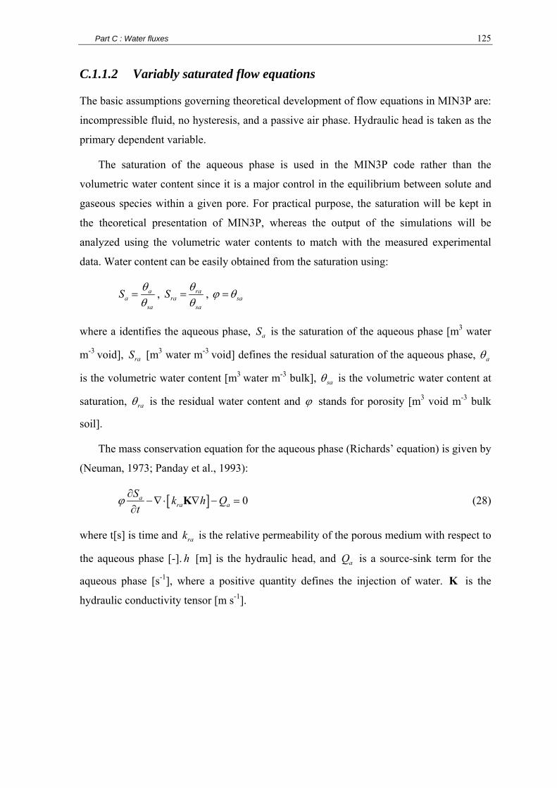
Part C : Water fluxes 125
C.1.1.2 Variably saturated flow equations
The basic assumptions governing theoretical development of flow equations in MIN3P are:
incompressible fluid, no hysteresis, and a passive air phase. Hydraulic head is taken as the
primary dependent variable.
The saturation of the aqueous phase is used in the MIN3P code rather than the
volumetric water content since it is a major control in the equilibrium between solute and
gaseous species within a given pore. For practical purpose, the saturation will be kept in
the theoretical presentation of MIN3P, whereas the output of the simulations will be
analyzed using the volumetric water contents to match with the measured experimental
data. Water content can be easily obtained from the saturation using:
aa
sa
S θθ
= , rara
sa
S θθ
= , saϕ θ=
where a identifies the aqueous phase, aS is the saturation of the aqueous phase [m3 water
m-3 void], raS [m3 water m-3 void] defines the residual saturation of the aqueous phase, aθ
is the volumetric water content [m3 water m-3 bulk], saθ is the volumetric water content at
saturation, raθ is the residual water content and ϕ stands for porosity [m3 void m-3 bulk
soil].
The mass conservation equation for the aqueous phase (Richards’ equation) is given by
(Neuman, 1973; Panday et al., 1993):
[ ] 0ara a
S k h Qt
ϕ ∂−∇⋅ ∇ − =
∂Κ (28)
where t[s] is time and rak is the relative permeability of the porous medium with respect to
the aqueous phase [-]. h [m] is the hydraulic head, and aQ is a source-sink term for the
aqueous phase [s-1], where a positive quantity defines the injection of water. Κ is the
hydraulic conductivity tensor [m s-1].

Part C : Water fluxes 126
C.1.1.3 Soil hydraulic parameters
Since the saturation and the relative permeability are a function of the aqueous phase
pressure, the equation mass is non linear. Relationships given by Mualem (1976) and Van
Genuchten (1980) are used to describe these dependencies.
( )1
1ra
a ra mna
SS Sαψ
−= +
+ (29)
( )2
1/1 1ml m
ra ea eak S S⎡ ⎤= − −⎢ ⎥⎣ ⎦ (30)
with
11mn
= − (31)
a h zψ = − (32)
1a ra
eara
S SSS−
=−
(33)
where α , n , m and l are the soil hydraulic function parameters, eaS is the effective
saturation of the aqueous phase, aψ [m] defines the pressure head of the aqueous phase
and z [m] is the elevation with respect to a given datum. When the soil is saturated, 1eaS = ,
1rak = , and thus Κ defines the hydraulic conductivity tensor at saturation. l is an
empirical pore tortuosity/connectivity parameter.
C.1.1.4 Evaporation and transpiration
The MIN3P evapotranspiration module was re-coded to ensure a better stability of the
model under more drastic conditions (water content close to the residual, high evaporation
or transpiration rates, high gradients of pressure head with rapid changes …) and to
differentiate evaporation from transpiration. The transpiration and evaporation models
already coded in MIN3P by F. Gerard and U. Mayer (Gerard et al., 2004) were kept and
their choice will not be discussed here but their mathematical translation was adapted.
The rate of water uptake and loss is calculated at each time step by adopting a method
similar to the one used in the soil water module SWIF of the FORHYD model (Tiktak and
Bouten, 1992). The mass balance equation for water in the forest ecosystem can be
expressed as:
max max max iET T EV f I= + + (34)
max maxinput
iT T f I= − (35)

Part C : Water fluxes 127
where ETmax is the maximum evapotranspiration [m s-1], Tmax is the maximum tree
transpiration rate [m s-1], maxEV corresponds to the sum of understorey plus soil
evaporation [m s-1], and I is the amount of intercepted water by the tree canopy [m]. The
correction of T by the if I term serves to take account of the tree transpiration reduction by
the evaporative demand of a wet canopy on days with precipitation. Tmax, EVmax and I are
input data at each time step t, fi is an input parameter specified for the whole simulation.
Both EVmax and Tmax are thereafter reduced by the water availability in the soil profile
at time t. Evaporation flux is calculated first considering that the trees may take up water
deeper in the soil profile in case of water deficiency in the surface layers. Evaporation over
bare ground involves very complex mechanisms of mass and heat exchanges at the
interface soil/atmosphere. Their numerical simulation requires very detailed models using
both a very short time step (namely of the order of 1 min) and large memory storage
(Mahfouf and Noilhan, 1991). Consequently, simple parameterizations and an explicit
formulation of the evaporation flux are required. Here, the effective evaporation rate EVeff
[m s-1] is calculated as (Wu et al., 1999):
max( , )eveff
AWEV Min EVt
=Δ
(36)
_( ) ( ) ( ) ( ( ) ( ))ev
ev ev a a dryi
AW vol i i R i S i S iϕ= ⋅ ⋅ ⋅ −∑ (37)
_
_
( ) ( )( ) ( ,1)
( ) ( )a a dry
evf a dry
S i S iR i Min
S i S i−
=−
(38)
where AWev [m3] is the water available for evaporation in the soil profile, Δt is the time
increment at time t of the simulation [s], iev indexes the soil profile cells which may
evaporate, vol(i) [m3] is the volume of cell i of the soil profile and φ(i) [-] its porosity,
Rev(i) [-] is a reduction factor which limits evaporation in cell i, Sa(i) is the saturation in
water of cell i, Sa_dry(i) its saturation for an air-dry pressure head (input parameter ψdry) and
Sf(i) its water saturation at a pressure head ψf (input parameter).
EVeff is then distributed in each cell of the soil profile proportionally to its saturation in
water:
_( ) ( ) ( )( ) ( ( ) ( ))ev
eff a a dry effev
vol i i R iEV i S i S i EVAWϕ⋅ ⋅
= ⋅ − ⋅ (39)

Part C : Water fluxes 128
It can be checked that ( )ev
eff effi
EV i EV=∑ .
After evaporation occurred, the remaining water AWtransp [m3] available for
transpiration in the soil profile is calculated by:
_ _ lim( ) ( ) ( ) ( ) ( ( ) ( ))transp
transp transp a postev ai
AW vol i i rld i R i S i S iϕ= ⋅ ⋅ ⋅ ⋅ −∑ (40)
_
( )( ) ( )
( )eff
a postev a
t EV iS i S i
iϕΔ ⋅
= − (41)
where itransp indexes the profile cells where transpiration may occur, rld(i) is a reduction
factor ≤ 1 which accounts for the root length density repartition in the soil profile, Rtransp(i)
is a reduction factor which limits the transpiration rate in cell i, Sa_postev(i) is the water
saturation in cell i once evaporation occurred, and Sa_lim(i) its water saturation for a given
pressure head ψlim (input parameter).
The effective transpiration is then calculated as:
max( , )transpeff
AWT Min T
t=
Δ (42)
Rtransp(i) is calculated according to Battaglia & Sands (1997) and distributed in each cell
using:
1
1 0 1
( )2
2 ( )20
( )( )( )
p REW i
transp p REW p REW i
REW i eR iREW e REW i e
⋅
⋅ ⋅
⋅=
⋅ + ⋅ (43)
_ _ lim
_ lim
( ) ( )( ) ( ,1)
( ) ( )a postev a
f a
S i S iREW i Min
S i S i−
=−
(44)
_ _ lim
( ) ( ) ( ) ( )( ) ( ( ) ( ))transp
eff a postev a efftransp
vol i i rld i R iT i S i S i T
AWϕ⋅ ⋅ ⋅
= ⋅ − ⋅ (45)
where REWi is the reserve of extractable water, REW0 and p1 are fitting parameters
( Figure 30).

Part C : Water fluxes 129
0.00
0.20
0.40
0.60
0.80
1.00
0 0.2 0.4 0.6 0.8 1
REW
R tra
nsp
0.29=Sa_dry 0.61 1
0.40 0.52
0.29 0.29
ψf=0 m
ψf=-1 m
ψf=-150 m
Saturation (m3water/m3
void)
— REW0=0.3, p1=2.5 --- REW0=0.3, p1=0.5 … REW0=0.3, p1=25
REW0
0.29=Sa_dry
0.29=Sa_dry
Figure 30 Influence of the transpiration parameters on the transpiration reduction factor Rtransp (eq (43)). Rtransp can be expressed as a function of the reserve of extractable water (REW) or as a function of the saturation in water Sa (eq (44)). Sa is controlled by ψf, the pressure head below which Rtransp≤1, and by ψlim, the pressure head below which the transpiration stops (fixed at -150 m in the figure). The curve shape is controlled by REW0
and p1 (eq (43)).

Part C : Water fluxes 130
C.1.1.5 Input and output
Table 23 MIN3P water balance module: inputs used in the simulations.
Input type Input parameters or variables Observations
Initial condition
Pressure head Each soil layer (core file), or each cell (external file)
Upper Flux (m s-1) Boundary conditions Lower Pressure head (m-1)
Time dependant, external file
α, n, m Retention curve Sra, Ssa
Soil hydraulic parameters
Hydraulic conductivity Ks, l Each soil layer, core file
Evaporation EVmax Time dependant, external file ψdry Each soil layer Evaporation depth Soil layers for which ψdry≠0
Transpiration Tmax Time dependant, external file p1, REW0 fi
Core file common to all soil layers
ψf, ψlim Core file, each soil layer
Source/sink term: evapotranspiration
rld Each cell (external file) or each soil
layer (core file)
Boundaries may be specified in MIN3P in terms of specified head boundary (pressure head
or hydraulic head), specified flux boundary or seepage face boundary, and can be constant
or time dependant. The initial conditions, the soil hydraulic parameters and the controls for
evapotranspiration must be specified as inputs in MIN3P ( Table 23).
Table 24 MIN3P water balance module: outputs used in the simulations. Output type Output Observation
Boundary fluxes Total inflow Total outflow Evapotranspiration fluxes Total evaporation Total transpiration
Mass balance
Change in soil water storage
At each time t from upper boundary to each observation node
Soil water saturation, water content, pressure head, interfacial velocities
For each node (x,y,z) at a given t For each t at a given node (x,y,z)
Soil profile snapshots
Evapotranspiration For each node (x,y,z) at a given t

Part C : Water fluxes 131
The main outputs of the water balance module of MIN3P are the water fluxes at the
boundaries and the effective transpiration and evaporation (total for the soil profile) at each
time step of the simulation. The model was also implemented to obtain these fluxes for
each observation node of the soil profile. Snapshots of the soil profile are also available for
some specified times t at each node of the soil profile ( Table 24).
C.1.2 General characteristics of the performed simulations
C.1.2.1 Main goals
The main goals of the modelling were to assess the water balance throughout the
experimental period, which meant to simulate daily outflow leaving the soil profile by
drainage (depth of 3 m) and by evapotranspiration (Teff and EVeff). The water flux for each
observation node also needed to be simulated to compute fluxes of nutrients in drainage
water.
Simulations were also performed to adjust parameters of the model which were not
experimentally acquired by optimizing the output of the simulations with the
experimentally measured water contents.
C.1.2.2 Time step
As TDR measurements and climatic data were available at least at a daily time step (see §
C.1.4 & C.1.3.2) and as our soil type is reported to drain very rapidly (Balbino et al., 2004;
Elsenbeer et al., 1999; Libardi, 2005; Paiva et al., 2000; Pochet et al., 2007), the water
drainage simulations were performed at a daily time step.
C.1.2.3 Monitoring period
The experimental period started in July 2003 and ended in April 2006 (7 months before
clear felling until 24 months after planting), which corresponds to three distinct
experimental periods : (i) before clear felling (BCF): from 09/07/2003 (Nday=1) to
14/02/2004 (Nday=221) included; (ii) after clear felling and before planting (CFP): from
20/02/2004 (Nday=227) to 22/04/2004 (Nday=289) included; (iii) after planting (AP): from
27/04/2004 (Nday=294) to 09/05/2006 (Nday=1036) ( Figure 6). Data until 05/08/2006

Part C : Water fluxes 132
(Nday=1124) were also used for the parameterization of the aboveground water fluxes
(stemflow and throughfall) models in ANNEX 4.
The BCF period was sub-divided in two periods BCF1 (dry) and BCF2 (wet) and the
CFP period was subdivided in CFP1 and CFP2. The AP period was divided in 6-month-
long sub-periods ( Figure 6).
C.1.2.4 Spatial unvariants: working hypotheses
Spatial heterogeneity of the transient water flow may result from heterogeneity of the
water inflow at the upper boundary of the soil profile or of the water uptake by
evapotranspiration, from spatial heterogeneity of the soil hydraulic properties, or from
preferential flow paths in the soil (through bio-channels for example). These
heterogeneities may occur at different scales and wide-range variability may be concealed
by short-range variability (Legout et al., 2008; McBratney et al., 2003). Many of the
manifestations of preferential flow and transport have their genesis at the upper boundary
of the soil profile (Clothier et al., 2008).
In the studied experiment, the water inflow is expected to vary (i) at the tree scale,
since the rainfall may be concentrated at the bottom of the tree stems by stemflow (Cattan
et al., 2007; Chang and Matzner, 2000; Johnson and Lehmann, 2006; Levia and Frost,
2003) or differentially transmitted by throughfall (Delphis et al., 2006; Konishi et al.,
2006; Levia and Frost, 2006), (ii) at the plot scale (intra plot, plot area = 600 m2) since
heterogeneities among the trees may modify these fluxes, and (iii) among the different
plots (inter plot, stand area = 1.8 ha) since differences in growth and/or soil characteristics
within the whole plot may also influence these fluxes. The spatial heterogeneity of rainfall
may also influence the inflow more probably at the inter or intra plot scale, since tropical
rain storms may occur locally (Levia and Frost, 2006). Differences in soil surface
characteristics (wettability) may also induce spatial heterogeneity of the inflow at a < 1 m
scale, especially for Eucalyptus forest floor which is well known for its hydrophobicity
(Laclau et al., 2004a).
Water uptake by trees is expected to vary at the tree scale since the root system of the
trees is spatially heterogeneous in the three dimensions of space, and at the intra-plot and
inter-plot scale since these root systems may differ from one tree or plot to another,
together with the water demand of the trees.

Part C : Water fluxes 133
For the studied ferralsols, part B showed that there was no significant intra or inter-plot
effect on major soil characteristics. The soil hydraulic properties are thus expected to be
quite homogeneous from one tree or plot to another. On the other hand, the micro
aggregation of this type of soil together with differences in the wettability of the soil
surfaces may induce heterogeneities of the soil hydraulic properties at a scale < 1 m
(Balbino et al., 2004; Cichota et al., 2006; Clothier et al., 2008; Elsenbeer et al., 1999;
Greiffenhagen et al., 2006; Laclau et al., 2004a; Paiva et al., 2000; Pochet et al., 2007).
The main goal of the present study was to estimate the water drainage leaving the soil
profile at a depth of 3 m at the plot scale. The working hypothesis was thus that the main
heterogeneities of the soil hydraulic properties occurred at a scale < 1 m and that taking
average soil hydraulic properties at this scale would allow a correct simulation of the soil
moisture at this scale too. A single average porosity was thus hypothesized. Once this
settled, heterogeneities of the water drainage due to heterogeneities of the inflow or of the
uptake may be simulated by changing the upper boundary or the uptake on a 1-D profile
under the hypothesis that lateral drainage is null. Such 1-D simulations do not allow the
construction of spatial maps of water drainage but may allow qualitative studies of the
different processes. 1-D simulations are easier to handle since they need less computing
power and model inputs. They were regarded sufficient within the scope of this study,
considering that the number of probes used to monitor soil water content was not sufficient
to validate a 2-D hydrological model. Preferential flow paths were not studied.
The simulations are thus performed for a vertical profile invariant according to the
horizontal plane, with a single average porosity. The water drainage only occurs vertically
which means that the lateral water movements are neglected. Since the slopes of the
experiment are flat and the soil quite homogeneous, the approximation seems reasonable.
C.1.2.5 Soil profile characteristics
The soil profile was deep of 3 m and composed of 4 layers:
• Layer 1: 0-30 cm observed at a depth of 15 cm
• Layer 2: 30-70 cm observed at a depth of 50 cm
• Layer 3: 70-230 cm observed at a depth of 150 cm
• Layer 4: 230-300 cm observed at a depth of 300 cm.
Part C : Water fluxes 134
The soil layers were defined from the pedological layers presented in part B: layer 1
corresponds to the soil layers greatly influenced by organic matter, layer 2 is a transition
layer between the soil layers influenced by organic matter and deeper soil layers for which
clay contents increase, layers 3 and 4 correspond to an increasing gradient of clay content.
As already mentioned in part B, the transitions between soil layers are gradual in this type
of soil and the main difference lies between the surface layers influenced by OM and the
deeper soil layers where clay contents are greatest (about 24%). Layer 4 was not included
in layer 3 because TDR measurements indicated wetter conditions at a depth of 3 m than at
a depth of 1.5 m (see § C.2.2). The observation nodes were located at the centre of the soil
layers except for layer 4 for which the observation node corresponded to the lower
boundary of the soil profile.
Although it has been shown that the Eucalyptus root structure develops deeper than 3
m (Knight, 1999; Laclau et al., 2001; Robinson et al., 2006), only a soil profile deep of 3 m
was studied. Water content measurements were available down to a depth of 3 m and so
were the soil solution samples. The stress was laid on evaluating with accuracy the water
fluxes in the soil profile between the surface and a depth of 3 m where most of the nutrient
uptake is expected to occur. It was thus considered essential to fix the lower boundary of
the profile as a measured value and not to introduce unknown variability in the simulations
from unknown and unobserved deeper soil layers.
In the model, the vertical profile was composed of 300 cells each one of dimension (1
m x 1 m x 0.01 m) in (x, y, z) from coordinates (1, 1, 0.01) to (1, 1, 3) and invariant
according to the plane (x, y) (1-D simulations).
C.1.2.6 Methodology
The first step was to assess which data may be used to calculate the time-dependant inputs
of the model, that is, data for the maximum evapotranspiration (outflow of the soil profile),
for the upper boundary (inflow) and the lower one (outflow) ( Table 23). The spatial
heterogeneity of the inputs thus obtained was discussed (§ C.1.3 & C.2.1, ANNEX 4). As
they will be used to assess the efficiency of the simulations, the water contents measured
on-site were also analyzed and their spatial heterogeneity discussed (§ C.1.4 & C.2.2).
Given the spatial heterogeneities observed, a general strategy was then decided whether to
test or not the influence of some heterogeneity among plots or treatments on the model
outputs (§ C.2.3).

Part C : Water fluxes 135
The input parameters which were not time dependant also needed to be set (§ C.1.5 &
C.2.4). The soil hydraulic properties were assessed for each soil layer. They were
considered invariant according to the horizontal plane (working hypothesis). The
parameterization of the input parameters driving the evapotranspiration was discussed.
The model was then used to adjust the evapotranspiration parameters which remained
unknown (§ C.1.6 & C.2.5): the CFP period was used to adjust the evaporation parameters
(no vegetation transpiration), the BCF period was used to adjust transpiration parameters
(mature Eucalyptus stand with a closed canopy), the AP period was a mixed between the
CFP and the BCF period and was used the check the validity of the model thus
parameterized. The sensitivity of the model to soil hydraulic properties, boundaries and
initial conditions was tested on the data from the CFP period.
Finally, the water fluxes leaving the soil profile at depths 15, 50, 100 and 300 cm were
calculated by running the model thus parameterized over the whole period (§ C.2.6).

Part C : Water fluxes 136
C.1.3 Time-dependant inputs of the model: daily maximum
evaporation and transpiration, and daily water inflow at the
soil surface
C.1.3.1 The transpiration term: evolution of the vegetation during the
studied period
The transpiration flux is defined by the water taken up by the vegetation and may be
influenced by changes in leaf area and stomatal regulation. The vegetation may also
influence the evaporation flux by changing the soil coverage and thus the energy reaching
the soil.
During the BCF1 and BCF2 period, the soil was covered by a mature stand of
Eucalyptus trees with a closed canopy. During the CFP period, the soil was covered by the
harvest residues of the clear felling of the BCF Eucalyptus stand and no vegetation was
present (use of glyphosate). During the AP period, a new Eucalyptus stand was planted and
managed according to 3 different silvicultures. This new stand grew rapidly and its canopy
was closed after 12 months of growth. The growth of the different stands was not studied
in the present work but some major data from Laclau et al. (2004b; 2005b; 2007) are
presented in the preamble of the thesis (Part A).
In MIN3P, the transpiration is regulated by (i) the daily maximum transpiration, (ii)
non-time dependant parameters regulating this maximum transpiration and (iii) the root
length densities (rld(z) of eq. (40)) which distribute the water uptake all along the soil
profile. The root length density profiles needed thus to be defined for the BCF and AP
periods (Eucalyptus trees). A classic exponential decay equation was fitted on the
experimental data already presented in part A and was used to compute root length
densities all along the soil profile:
( )( ) exprld rld rldRLD z A B C z= + − (46)
where RLD is the root length density, z the depth in cm and Arld, Brld, Crld the parameters to
be fitted. This root length density needed to be normalized to match the model input
format, which was done by:
( )( ) exprld rld rldrld i a b c i= + −

Part C : Water fluxes 137
, , rld rldrld rld rld rld
rld rld rld rld
A Ba b c CA B A B
= = =+ +
(47)
where rld(i) is the root length density input for cell i, and Arld, Brld, Crld the fitted
parameters of equation (46).
Using a continuous function was preferred to the discontinuous experimental data
since: (i) gradual decrease of the root length density was observed during the pedological
descriptions (part B), (ii) it allows simple comparisons among the root length density
profiles by analyzing the fitted parameters, (iii) and such functions are necessary to
implement the model with a root growth module if needed.
C.1.3.2 Meteorological data
The effective transpiration may be experimentally measured by monitoring xylem sap
fluxes (Granier, 1987). Together with the monitoring of soil water content and of
meteorological data, it allows the experimental calibration of the parameters controlling
transpiration (reduction factor RT) (Granier et al., 1999a). This study was at its beginning
in the experimental area when the present work was realized so that the maxima plant
uptake (transpiration) and soil evaporation needed to be estimated from meteorological
data. The parameters driving the transpiration had to be either fixed using the literature or
optimized by simulation.
Available meteorological data were weekly rainfall (Pi) in a 1 ha opened area next to
the experimental site, daily rainfall (Piref) and temperature (minimum, maximum, average)
at 2 km from the experimental site (Itatinga, SP), global radiation, wind velocity, insolation
and relative water content at about 20 km from the experimental site (meteorological
station of UNESP, Botucatu, SP) ( Table 25). On-site daily rainfall will thus have to be
estimated from on-site weekly measurements and from the daily Piref. The calculation is
given in ANNEX 4. The maximum evaporation and transpiration will have to be estimated
from the Botucatu data.

Part C : Water fluxes 138
Table 25 Monitored fluxes: number of collectors and time steps of data acquisition. Type of collecting device Location Abbreviation Number Time step
Rain Gauge Open area next to experimental site Pi 1 Weekly Itatinga (2 km) Piref 1 Daily Total depositions Open area next to experimental site Thref 1 Weekly Throughfall On site Th 9 Weekly Stemflow On site St BCF 8 Weekly A
bove
gro
und
fluxe
s
AP 27 Weekly
Soil
wat
er
mon
itorin
g TDR probes On site, at depths of: 15 cm 50 cm 150 cm 300 cm
9 9 9 9
Every 12 hours
Global radiation, wind velocity, insolation and relative water content
Botucatu (20 km) Daily
Met
erol
ogic
al
data
Temperature (maximum, minimum, average)
Itatinga (2 km) Daily
Penman Monteith equation (Monteith, 1981) is commonly used to calculate maximum
evapotranspiration from weather data:
( ) ( )( )
/11 /
n a p s a a
s a
R G c e e rET
r rρ
λ γΔ − + −
= ⋅Δ + +
(48)
where Rn is the net radiation, G is the soil heat flux, (es-ea) represents the vapour pressure
deficit of the air, ρa is the mean air density at constant pressure, cp is the specific heat of the
air, Δ represents the slope of the saturation vapour pressure temperature relationship, γ is
the psychrometric constant, and rs and ra are the (bulk) surface and aerodynamic
resistances. These resistances are vegetation specific. Aerodynamic resistance determines
the transfer of heat and water vapour from the evaporation surface into the air above the
canopy and is calculated from wind and water content measurements. ‘Bulk’ surface
resistance describes the resistance of vapor flow through the transpiring vegetation and
evaporating soil surface.
The surface resistance was undefined for the soils and the Eucalyptus vegetation of the
experiment and the available meteorological data were obtained at 20 km far from the
experimental site and in tropical climates, weather changes may occur at short range. The
maximum evaporation and transpiration needed thus to be adjusted to on-site conditions.
Two types of evapotranspiration were calculated for this purpose. The first one was the

Part C : Water fluxes 139
reference FAO evapotranspiration (ETref) which is the evapotranspiration for a
hypothetical reference crop of height 0.12 m, surface resistance 70 s m-1 and albedo 0.23. It
closely resembles the evaporation of an extension surface of green grass of uniform height,
actively growing and adequately watered. It was used to compare our results to a standard
evapotranspiration and was computed thanks to the FAO Penman-Monteith method as
(Allen et al., 1998):
( ) ( )( )
2
2
0.408 ( ) 900 / 2731 0.34
n s aref
R G T u e eET
uγγ
⋅Δ ⋅ − + ⋅ + ⋅ −=
Δ + + ⋅ (49)
with ETref the reference evapotranspiration [mm day-1], Rn the net radiation at the crop
surface [MJ m-2 day-1], G the soil heat flux density [MJ m-2 day-1], T the mean daily air
temperature at 2 m height [°C], u2 the wind speed at 2 m height [m s-1], es the saturation
vapour pressure [kPa], ea the actual vapour pressure [kPa], (es-ea) the saturation vapour
pressure deficit [kPa], Δ the slope of the saturation vapour pressure temperature
relationship [kPa °C-1] and γ the psychrometric constant [kPa °C-1].
An evaluation of the maximum energy available for evapotranspiration (ETmax) was
also performed using Penman Monteith equation with rs set to its minimum (rs=0 in eq
(48)) and Rn maximum (albedo=0). ETref was used to test different levels of maxima
evaporation (EVmax) and transpiration (Tmax). Once limited by the water availability in the
soil profile, EVmax and Tmax constitute the effective transpiration (Teff) and evaporation
(EVeff) computed as outputs by the water drainage model.

Part C : Water fluxes 140
C.1.3.3 Inflow at the upper boundary of the soil profile: throughfall,
stemflow and surface run-off
Figure 31 Aboveground water fluxes collectors: stemflow (A); throughfall (B) and surface run-off (C).
The water inflow at the upper boundary of the soil profile (Psoil) and the interception
term (I) are inputs of the model. Psoil is the upper boundary and I participates in the
transpiration calculation. For forest ecosystems, they are classically calculated as:
=soilP Th St Ru+ − (50)
I Pi Th St= − − (51)
where Th stands for throughfall, St for stemflow and Ru for surface run-off.
Throughfall solutions were measured weekly in collecting devices made of 12 funnels
systematically distributed beneath the trees to integrate the heterogeneity at the tree scale
( Figure 31). Nine replicates of collecting devices were monitored before clear-felling to
check the inter plot spatial heterogeneity. Then, one collecting device per experimental plot

Part C : Water fluxes 141
in treatment 1, 3 and 5 and blocks 1, 2 and 3 was monitored (total of 9 devices) after trees
had reached a sufficient height (10 months after planting in block 1 and 14 months after
planting in blocks 2 and 3).
Stem flows (St) were collected from helical collars installed on trees (Marques, 1996)
and measured weekly in a collection bucket (St[mL]) ( Figure 31). Before clear felling,
eight of these collars were installed on trees representative of the stand. After clear felling,
stem flow collecting devices were installed in January 2006 (20 months after planting)
around 3 trees per experimental plot (blocks 1, 2 and 3 of treatments 1, 3 and 5 of the
fertilization experiment).
Surface runoff was measured and collected weekly in each treatment from one 3x2 m
collector.
Throughfall, stemflow and surface run-off were measured weekly. As the model
operates at a daily time step, they needed to be estimated daily. This calculation together
with the analysis of the spatial heterogeneity of these fluxes is detailed in ANNEX 4. It
was placed in annex since material, methods and results were frequently inter-related in
these calculations.

Part C : Water fluxes 142
C.1.4 Data used to assess the simulations’ efficiency: soil water
monitoring
Soil moisture was measured every twelve hours (except in case of equipment failure)
thanks to TDR probes (Time Domain Reflectometry) installed at the depths of 15, 50, 150
and 300 cm. The probes were installed at 3 distances from the planting row (close to an
average tree, ¼ and ½ of the inter-row) at each depth in 3 plots. Before clear felling, these
3 plots were independent repetitions. After clear felling, the three plots corresponded to
block 1 of treatments 1, 3 and 5, where the lysimetric design was installed ( Figure 4 &
Figure 5). Daily data were obtained by calculating the average water contents measured for
the current day.
The water content measured by each probe was compared to the average value
obtained for all TDR probes at a fixed depth by linear regression using proc GLM of SAS
Software (www.sas.com). The linear regressions thus obtained were used to study the
spatial heterogeneity of the measured water contents. In particular, the effects of block and
treatment were tested on the intercepts by ANOVA analysis (proc GLM) to test the
hypothesis of systematic wetter or dryer water contents in some block or treatment.

Part C : Water fluxes 143
C.1.5 Non time-dependant inputs of the model
C.1.5.1 Parameters regulating transpiration
REW0, p1, ψlim, ψf, and f1 still remained to be set. Litterature reports values of REW0 of 0.3
or 0.4 for other tree species (Battaglia and Sands, 1997; Granier et al., 2007; Kirschbaum
et al., 2007) and p1=2.5, ψf is classically set to -1 (field capacity) and ψlim to the wilting
point (Battaglia and Sands, 1997). As Eucalyptus trees are reported to be highly efficient in
their water consumption and as very low water contents were reached during the
experimental period (down to residual water contents) suggesting that Eucalyptus trees
could extract water down to very low absolute potentials, we chose to fix ψlim down to the
residual water content and to optimize the others parameters together with Tmax using the
data of the very dry period BCF1.
The values of f1 used in the literature range from 0.14 to 0.2 (Gerard et al., 2004;
Tiktak and Bouten, 1994). This parameter was not optimized since it affects the
interception term which was low in the studied stand (cf C.2.1.3) and may thus not
influence much the simulations. It was set to 0.2.
C.1.5.2 Soil hydraulic parameters: transient flow experiment
C.1.5.2.1 Transient flow experiment
Characterization of soils and the vadose zone includes the estimation of the soil water
retention and unsaturated hydraulic conductivity relations for a wide range of volumetric
water content values. Although laboratory experiments have the advantage of being quick
and precise, they often lead to soil hydraulic properties that are not representative of the
field. Among available field experimental procedures, transient experiment and inverse
modelling approach allow the simultaneous estimation of both the soil water retention and
the unsaturated hydraulic conductivity function (Hopmans et al., 2002; Vachaud and Dane,
2002). An inverse method includes three interrelated functional parts: (i) a controlled
transient flow experiment for which boundary and initial conditions are prescribed and
various flow variables are measured; (ii) a numerical flow model simulating the transient
flow regime of this experiment; (iii) and an optimization algorithm, which estimates the
unknown parameters through minimization of the difference between observed and

Part C : Water fluxes 144
simulated flow variables. Among the benefits of inverse methods is the fact that they are
equally applicable to field experiments, even under nontrivial boundary conditions. The
difficulty of the inverse resolution is that the solution is generally non-unique and is highly
dependant upon the initial set of parameters chosen (Hill, 1998). This approach was used
here and adapted to the model requirements.
The transient flow experiment chosen was that of the instantaneous profile (also
known as internal drainage method) which is considered a standard (Hopmans et al., 2002;
Vachaud and Dane, 2002). It was conducted between clear felling and planting (from
20/04/2004 till 23/04/2004) on a 15 m2 vegetation-free plot of block 1 of treatment 3. The
area was set superior to 12 m2 to limit the relative importance of lateral water movement at
the plot boundary. Its centre was positioned above the 3 replicates of TDR probes installed
8-months earlier in this plot at depths 15 cm, 50 cm, 150 cm, 300 cm. The plot was further
instrumented in its centre with tensiometers at depths 15 cm, 50 cm, 1 m, 1.50 m, 2 m, 2.50
m and 3 m.
The experiment was initiated by pounding water over the entire plot area until pressure
head values were approximately zero or did not change with time down to a depth of 3m.
After the water supply was stopped and the pounded water had infiltrated, the plot was
covered with a plastic sheet and insulated to ensure a zero-flux top boundary condition and
to reduce temperature variations ( Figure 32). Subsequently, the soil was allowed to drain
by gravity. The transient drainage process was monitored by simultaneous measurements
of soil water content and pressure head every half hour in the first day of the experiment,
and then daily until the end of the internal drainage experiment.
Figure 32 Interval drainage experiment (a) during pounding (b) during transient drainage (the plastic sheet ensures a zero-flux top boundary).

Part C : Water fluxes 145
The estimation of the unknown soil hydraulic parameters was not performed thanks to
an inversion procedure stricto senso because MIN3P did not have an inverse procedure.
The inverse procedure of Hydrus 1D (www.pc-progress.cz/Pg_Hydrus_1D.htm) was tested
but was unstable with our data set. The calculation of the water retention curve and the soil
hydraulic conductivity parameters is explained thereafter.
C.1.5.2.2 Water retention curve parameters
Water retention curve parameters (α , n , m , raθ and saθ ) were estimated for each soil
layer from the water contents and the pressure heads experimentally acquired during the
internal drainage experiment at depths 15 cm, 50 cm, 150 cm and 300 cm. As the
experimental data at high absolute pressure heads were scarce, raθ ( lima aψ θ→∞ ) was set as
the average of the driest water contents reached from July 2003 to September 2006 in each
block and treatment for each depth. saθ was set as the volumetric water content measured
at t=0 during the drainage experiment at each monitored depth. α , n , m were fitted using
the software SWRC (Dourado-Neto et al., 2001).
C.1.5.2.3 Hydraulic conductivity parameters
Hydraulic conductivity parameters (Ks and l) were calculated to minimize the difference
between simulated data by MIN3P and experimental records of the drainage experiment.
The top boundary flux (z=0) was set to zero (no evapotranspiration, no rainfall), and the
initial condition (t=0) taken as the soil profile fully saturated ( ( ) 0 0 3a z z mψ = ∀ ≤ ≤ ). Ks
and l were considered constant within a homogeneous soil layer. The studied soil layers
were as presented in § C.1.2.5.
The numeric problem was complex. It was constituted of 8 parameters taken
independently (Ks and l for each studied layer) but interactions between these parameters
may influence each layer response. In order to estimate such influences, a statistical model
based on Design Of Experiments (DOE) has been designed to determine the effects of the
various factors. At a first level of modeling, DOE supposed linear influence of each
parameter on each output. Deviations to linearity are taken into account by the introduction
of interactions among the studied factors (Sabre, 2007; Taguchi, 1986).
For each time t and layer k, the simulated water content is supposed to be a linear
response of the eight factors Ksi li and without interaction:

Part C : Water fluxes 146
( ) 1 2 3 4 5 6 7 8, 1 4 1 4 , , 1 , 1 , 2 , 2 , 3 , 3 , 4 , 4, = average
k t i i k t k t k t k t k t k t k t k t k tKs l x Ks x l x Ks x l x Ks x l x Ks x lθ θ≤ ≤ ≤ ≤ + + + + + + + +
(52)
Under some conditions of orthogonality, the }{ , 1 8
ik t i
x≤ ≤
and ,averagek tθ may be calculated
from a minimum set of simulations (experiment matrix) using combinations of extrema
values of the eight factors 1 4 1 4,i iKs l≤ ≤ ≤ ≤ (Taguchi, 1986). Then, eight observed values of
,k tθ allow the calculation of }{ 1 4,i i i
Ks l≤ ≤
by solving the matrix equation
, , ,= ,average ik t k t k t i i+θ θ x Ks li . The difficult step is to establish the extrema values of the eight
factors that will be used in the matrix of experiment due to the quasi linearity supposed by
the DOE theory. Deviations to linearity are taken into account introducing interactions
among the studied factors. The choice of the matrix depends on the complexity of the
model supposed by the user. In this case, it can be shown that a 16x8 matrix enables the
study of a model with 8 parameters and 4 independent interactions (Taguchi, 1986).
The matrix used comported 2 levels of factors (minimum, maximum), eight columns
(8 factors) and 16 lines (L16(28)) (Taguchi, 1986). In a second step of calculation, another
table was used L8(27) which did not use the Ks4 factor.
Preliminary studies (trial and error) helped us define the extrema:
• Ks1min=9 10-5 m s-1, Ks1
max=15 10-5 m s-1, l1min=3, l1
max=5
• Ks2min=10 10-5 m s-1, Ks2
max=20 10-5 m s-1, l2min=3, l2
max=7
• Ks3min=5 10-5 m s-1, Ks3
max=10 10-5 m s-1, l3min=2, l3
max=4
• Ks4min=1.5 10-5 m s-1, Ks4
max=4 10-5 m s-1, l4min=0.5, l4
max=4
The simulated water contents were observed at t=1 hour and t=4.5 hours for layers 1
and 2, and at t=1.5 hour and t=4.5 hours for layer 3 and t=2.5 hour and t=4.5 hour for layer
4 (8 responses of water content). The first time of observation was different for layers 3
and 4 since a slight delay occurred before the discharge of these layers began.

Part C : Water fluxes 147
C.1.6 Simulations
C.1.6.1 Efficiency of the simulations
For all simulations, the linear regressions of simulated against measured water contents
were fitted at each observation depth. The efficiency of the simulation was evaluated
through the sum of square of the simulated against the measured data. Two efficiency
coefficients were defined:
( )( )( )
2
, , , ,n 2
, , , ,
EFF1 =1-simulated measuredn k t n k tk t
simulated measuredn k t n k tk tn
Max
θ θ
θ θ
−
−
∑ ∑∑ ∑
(53)
( )( )( )
2
, , , ,n 2
, , , ,
EFF2 =1-simulated measuredn k t n k tk t
simulated measuredn k t n k tk tn
DM DM
Max DM DM
θ θ
θ θ
−
−
∑ ∑∑ ∑
(54)
with
, , , , ,n k t n k t n kDMθ θ θ= −
where k are the monitored depths (15 cm, 50 cm, 150 cm, the 300 cm observation node is
the lower boundary) and t the output times of the simulation, n indexes the performed
simulation, , ,n k tθ are the measured and simulated water content for the simulation n,
observation node k and time t and
,n kθ is the average water content for all times t of the
simulation n, observation node k. ( )2
, , , ,simulated measuredn k t n k tk t
θ θ−∑ ∑ is the sum of square errors
for all layers k and times t of the simulation n. ( )2
, , , ,simulated measuredn k t n k tk t
DM DMθ θ−∑ ∑ is the
sum of square errors of the deviation to the mean water content for all layers k and times t
of the simulation n.
EFF1 and EFF2 were defined so that: 0≤EFF≤1. A perfect fit is indicated by
EFF1=EFF2=1, and the worst fit by EFF1=0 and/or EFF2=0. EFF2 was introduced to
assess the efficiency of the fit regardless of the bias of the simulation. EFF1 and EFF2
were built as tools to help comparing the simulations within a given set of simulations
(maxima defined within this simulation set) but do not allow comparing the simulations
among different sets of simulations (different maxima).

Part C : Water fluxes 148
C.1.6.2 CFP period: fit of the evaporation term
During this period, the transpiration term was null (no trees thus no uptake) and the water
uptake from the soil profile by evapotranspiration was evaporation so. Evaporation
parameters (EVmax and evaporation depth) were adjusted to optimize the simulations
against the measured values on the first 33 days of the period (CFP1) when water content
measurements were available.
Levels of maximum evaporation tested were EVmax= fEV ETmax, with fEV∈{0.1 0.2 0.3
0.4 0.5 0.6 0.7 0.8 0.9 1}. Evaporation depths tested were: zEV∈{1 5 10 15 20 25 30} in
cm. All in all, 70 simulations were performed ( Table 26).
C.1.6.3 BCF period: fit of the transpiration term
Table 26 Values tested for the input parameters regulating transpiration and evaporation fluxes in the model. Each parameter is presented in § C.1.1.
Parameter Tested values Soil layer Time period
Evaporation fEV 0.1 ; 0.2 ; 0.3 ; 0.4 ; 0.5 ; 0.6 ; 0.7 ; 0.8 ; 0.9 ; 1 common ψdry -150 m each zEV (cm) 1 ; 5 ; 10 ; 15 ; 20 ; 25 ; 30 common
CFP
Transpiration fT 0.1 ; 0.2 ; 0.3 ; 0.4 ; 0.5 ; 0.6 ; 0.7 ; 0.8 ; 0.9 ; 1 common BCF2 p1 0.1 ; 2.5 ; 25 common REW0 0.1 ; 0.3 ; 0.5 ; 0.7 ; 0.9 common fi 0.8 common ψf 0 m ; -1 m ; -150 m each ψlim -150 m each rld Eq 47 each cell
BCF1
The BCF period represents a pole of mature Eucalyptus with a closed canopy. Only a
transpiration term was considered during this period, which was in fact the sum of an
evaporative flux and a predominant transpiration flux. The level of maximum transpiration
was adjusted during the BCF2 period when absolute pressure heads were < 1 m (rainy
period, classically no regulation of the transpiration for these pressure heads). The
maximum transpiration levels tested were of Tmax= fT ETmax, with fT∈{0.1 0.2 0.3 0.4 0.5
0.6 0.7 0.8 0.9 1} ( Table 26).
The parameters regulating transpiration were subsequently optimized during the BCF1
period when few rainy events and very low pressure heads (drying) occurred, using the
retained level of ETmax. The limit pressure head for which no more transpiration occur ψlim

Part C : Water fluxes 149
was fixed at -150 m for all layers. Since the residual water content is reached for a pressure
head of – 5 m, this means that the pressure head below which Eucalyptus uptake stops was
entirely controlled by the reduction factor RT and thus by the REW0, p1 and ψf parameters
( Figure 30) and not by the ψlim parameter.
The parameters controlling the transpiration are more or less redundant and that is why
ψlim was not optimized. Yet, altering ψf is the only way to introduce differences among soil
layers in the regulation of the transpiration. ψf controls the threshold pressure head below
which the transpiration is regulated by the RT coefficient ( Figure 30). ψf was optimized
because Eucalyptus trees are reported to be very efficient in their water uptake and may
uptake water down to very low pressure heads. Moreover, the retention curves for this soil
type are steep and the classically used ψf=-1 m may underestimate the regulation threshold
in terms of water contents (water content varying quickly with pressure head in this zone
of the water retention curve).
Three values of ψf were tested: ψf [m] ∈ {0 -1 -150} ( Table 26). ψf=0 means that the
transpiration is always regulated, ψf=-1 m corresponds to the soil field capacity and is the
value classically used (Battaglia and Sands, 1997), and ψf=-150 m means that the
transpiration is never regulated in the soil layer. ψf was also used to test the heterogeneity
of the regulation among soil layers. This heterogeneity may result from an underestimation
of the residual water content for deep soil layers which rarely dry, and/or from a
preferential uptake in these deep and wet soil layers when the upper soil layers dry. The
number of simulations was reduced considering that |ψf| for a given soil layer was
necessarily ≥ than |ψf| of the soil layer right above.
The parameters controlling the regulation curve REW0 and p1 were also adjusted. The
range of theoretical variations for REW0 is [0 1] so that five evenly distributed values were
tested: REW0 ∈ {0.1 0.3 0.5 0.7 0.9}. The theoretical range of variation of p1 is [0 +∞[. 3
values were tested: p1 ∈ {0.5 2.5 25}, where 2.5 is the value used by Battaglia for other
tree species (Battaglia and Sands, 1997) and 0.5 and 25 were used to test the effect of large
modifications of this value ( Table 26).

Part C : Water fluxes 150
C.1.6.4 AP period: model validation
The AP period (after planting) was used to check the validity of the parameterization of
both evaporation and transpiration parameters. This period corresponds to the first two
years of growth of the newly planted Eucalyptus stand.
Since Tmax for the 6-months-old Eucalyptus trees must be less than Tmax after canopy
closure at 12 months after planting, Tmax needed to be reduced by a function of the stand
growth. As transpiration is reported to vary with leaf area index (LAI) (Granier et al.,
1999b; Stape et al., 2004; Whitehead and Beadle, 2004), LAI was used to reduce Tmax
input in the model.
Even if the mathematical dimension of leaf surface (from which LAI is derived) is an
area (m2), leaves grow on tree in the three dimensions of space. Supposing that the water
uptake by the trees (and thus tree growth) may be modelled by a one-dimension function,
LAI would then be related to the cube of this function. A simple reduction function of
(LAI)1/3 fitted on the data presented in part A was thus tested to reduce Tmax during the AP
period:
max max( ) ( ) APT t RF LAI T= (55)
( ) ( )1/3
1/3
LAIRF LAIMax LAI
= (56)
where RF(LAI) (0≤RF(LAI)≤1) is the reduction function of the transpiration term
( Figure 33) and maxAPT the maximum level of transpiration for a reduction of factor of 1
during the AP period. The resulting function was in good agreement with similar
observations made by Granier et al. (2007; 1999b).
Since the new stand was more efficiently fertilized than the BCF one, the LAI for the
AP period were greater than that for the BCF one. The reduction curve of Figure 33 gives
the RF factor corresponding to the LAI of the BCF period. maxAPT was then calculated as:
maxmax
( )AP BCFBCF
RF LAITT
= (57)
The evaporation term was considered to decrease linearly from the planting (EVmax
parameterized during the CFP period) to the canopy closure occurring at 12 months old
(EVmax=0).

Part C : Water fluxes 151
0.0
0.2
0.4
0.6
0.8
1.0
0 200 400 600 800 1000
Time after planting (days)
RF
BCF
AP
T max
0.8 ETmax
0.6 ETmax
Figure 33 Time course of the RF factor (eq. (55) & (56)) reducing the maximum transpiration (Tmax) over the AP period. The corresponding Tmax for the BCF and the AP periods are given.
C.1.6.5 Sensitivity tests
The model sensitivity to soil hydraulic parameters, boundaries and initial conditions was
tested on the CFP period (no Eucalyptus) with the evaporation term set to zero. Table 27
gives the values of each input parameter or variable. Each one of these values was tested
with all other variables and parameters set to its average value. The range of variation of
water contents (θa) (and of their derived pressure heads ψa) was set to θa ± 1 %. The rainfall
(Pi) range of variation was set to Pi ± 0.25 Pi. The Ks range of variation for the 0-5 cm
layer was Ks/2<Ks<2Ks. For all other soil hydraulic parameters, the range of variation was
taken as ± 10% of the parameter value for the 0-5 cm layer.
For water content and rainfall, the range of variation corresponded to the average
variability observed in the experimental data sets ( C.2.2). For other parameters, it was
difficult to assess the variability which may be expected and the range of variation of ±
10% was arbitrary tested. For Ks, the literature reports differences of up to ten times when
measured by different experimental methods (Reynolds et al., 2002). The range of
variation was thus broadened to [Ks/2 2 Ks].

Part C : Water fluxes 152
Table 27 Parameter values used for the sensitivity tests. The parameters are explained in (§ C.1.1.4).
Studied parameters Lower value Average value Upper value Observations
Boundaries Upper: inflow 0.75 Pi Pi 1.25 Pi 0 cm Lower: pressure head ψa(θa(300cm)-1) ψa(θa(300cm)) ψa(θa(300cm)-1)) 300 cm
Initial condition Pressure head ψa(θa-1) ψa(θa) ψa(θa+1) All layers
0.9 α α 1.1 α 0.9 n n 1.1 n θra-1 θra θra+1
Retention curve parameters
θsa-1 θsa θsa+1
0.5 Ks Ks 2 Ks Velocity parameters 0.9 l l 1.1 l
Soil hydraulic parameters
0-30 cm layer
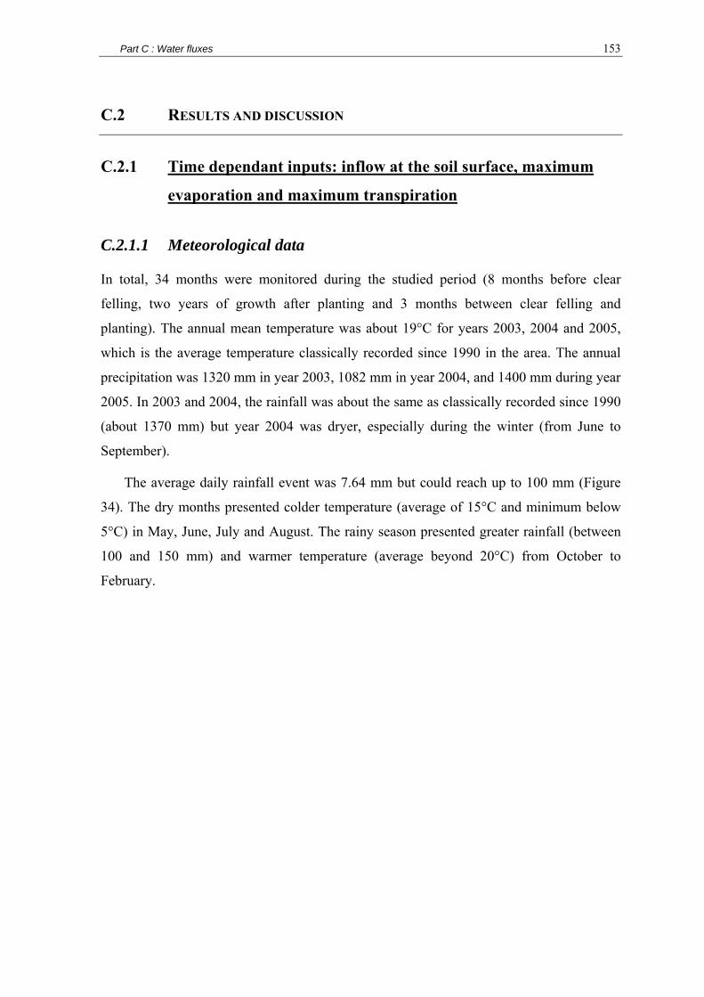
Part C : Water fluxes 153
C.2 RESULTS AND DISCUSSION
C.2.1 Time dependant inputs: inflow at the soil surface, maximum
evaporation and maximum transpiration
C.2.1.1 Meteorological data
In total, 34 months were monitored during the studied period (8 months before clear
felling, two years of growth after planting and 3 months between clear felling and
planting). The annual mean temperature was about 19°C for years 2003, 2004 and 2005,
which is the average temperature classically recorded since 1990 in the area. The annual
precipitation was 1320 mm in year 2003, 1082 mm in year 2004, and 1400 mm during year
2005. In 2003 and 2004, the rainfall was about the same as classically recorded since 1990
(about 1370 mm) but year 2004 was dryer, especially during the winter (from June to
September).
The average daily rainfall event was 7.64 mm but could reach up to 100 mm ( Figure
34). The dry months presented colder temperature (average of 15°C and minimum below
5°C) in May, June, July and August. The rainy season presented greater rainfall (between
100 and 150 mm) and warmer temperature (average beyond 20°C) from October to
February.

Part C : Water fluxes 154
0
100
200
300
7 8 9 10 11 12 12.
12.
2 3 4 5 6 7 8 9 10 11 12 12.
12.
2 3 4 5 6 7 8 9 10 11 12 12.
12.
2 3 4 5 6 7 8 9
2003 2004 2005 2006
Rai
nfal
l (m
m)
Stemflow Throughfall Interception
0
10
20
30
40
7 8 9 10 11 12 12.
12.
2 3 4 5 6 7 8 9 10 11 12 12.
12.
2 3 4 5 6 7 8 9 10 11 12 12.
12.
2 3 4 5 6 7 8 9
2003 2004 2005 2006
Tem
pera
ture
(°C
)
Average Maxima Minima
Clear felling Plantation Installation of throughfall collecting devices
Installation of stemflow collecting devices
0
100
200
300
7 8 9 10 11 12 12.
12.
2 3 4 5 6 7 8 9 10 11 12 12.
12.
2 3 4 5 6 7 8 9 10 11 12 12.
12.
2 3 4 5 6 7 8 9
2003 2004 2005 2006
Evap
otra
nspi
ratio
n (m
m)
ETmax ETref
Figure 34 Time course of temperature, rainfall and evapotranspiration (ET) over the time of the experiment. The rainfall partition between stemflow, throughfall and interception is given. From 02/2004 to 02/2005, interception represents rainfall since throughfall was not monitored during this period (young Eucalyptus trees). The maximum evapotranspiration (ETmax) and the FAO reference evapotranspiration (ETref) are given.

Part C : Water fluxes 155
The calculated evapotranspirations (ETmax and ETref) were minima in May and June
during the dry and cold months with values of about 50 to 70 mm month-1 for ETref and
ETmax ( Figure 34). They were maxima during the wet and warm months with values
reaching 110 mm month-1 for ETref and 170 mm month-1 for ETmax. Daily ETmax was in
average 4.38 mm day-1 and ETref 2.81 mm day-1. ETref was linearly correlated to ETmax (r2
= 0.98) and was about 64 % of ETmax.
The calculated evapotranspirations were of the same order of magnitude than the
rainfall during the wet months and largely greater than rainfall during the dry season. In the
presence of vegetation, the drainage is thus expected to be limited, especially during the
dry months when soil drying is to be expected.
C.2.1.2 Root length density
The fitted parameters for equation (47) describing the root length density repartition with
depth for the different time periods are given in Table 28. Figure 35 shows the fitted
function against the measured data at the end of the rotation of the old Eucalyptus stand
(BCF period).
Table 28 Parameters of the root length density model over the studied period. Period age (months) arld brld crld
BCF 72 0.018 0.982 0.054
4 0.045 0.955 0.049 6 0.044 0.956 0.054
12 0.081 0.919 0.048 22 0.051 0.948 0.058
AP
average 0.055 0.945 0.052
For the new stand planted in 2004 (AP period), the fitted curves once normalized were
more or less the same for all ages so that only an average curve was used as input for the
simulations.
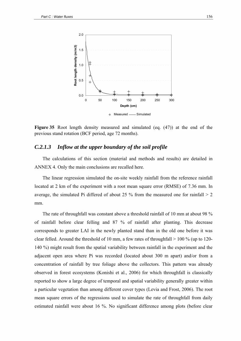
Part C : Water fluxes 156
0.0
0.5
1.0
1.5
2.0
0 50 100 150 200 250 300
Depth (cm)
Roo
t len
gth
dens
ity (m
/m3)
Measured Simulated
Figure 35 Root length density measured and simulated (eq. (47)) at the end of the previous stand rotation (BCF period, age 72 months).
C.2.1.3 Inflow at the upper boundary of the soil profile
The calculations of this section (material and methods and results) are detailed in
ANNEX 4. Only the main conclusions are recalled here.
The linear regression simulated the on-site weekly rainfall from the reference rainfall
located at 2 km of the experiment with a root mean square error (RMSE) of 7.36 mm. In
average, the simulated Pi differed of about 25 % from the measured one for rainfall > 2
mm.
The rate of throughfall was constant above a threshold rainfall of 10 mm at about 98 %
of rainfall before clear felling and 87 % of rainfall after planting. This decrease
corresponds to greater LAI in the newly planted stand than in the old one before it was
clear felled. Around the threshold of 10 mm, a few rates of throughfall > 100 % (up to 120-
140 %) might result from the spatial variability between rainfall in the experiment and the
adjacent open area where Pi was recorded (located about 300 m apart) and/or from a
concentration of rainfall by tree foliage above the collectors. This pattern was already
observed in forest ecosystems (Konishi et al., 2006) for which throughfall is classically
reported to show a large degree of temporal and spatial variability generally greater within
a particular vegetation than among different cover types (Levia and Frost, 2006). The root
mean square errors of the regressions used to simulate the rate of throughfall from daily
estimated rainfall were about 16 %. No significant difference among plots (before clear

Part C : Water fluxes 157
felling) and among treatments (after planting) was observed. This is in good agreement
with the homogeneity of the LAI observed among the different treatments once the canopy
closed (about age 12 months, when the monitoring of throughfall started).
The stemflow volume collected on individual trees was less for small trees and low
rainfall intensity and greatest at a constant value of about 37 L week-1 for circumference at
breast height (CBH) > 8 cm and rainfall > 50 mm. In-between, the stemflow increased
together with CBH and rainfall intensity. Daily stemflow for each tree of the experiment
was estimated from its CBH at the latest inventory and from the daily estimated rainfall
using a mathematical function fitted on weekly stemflows and rainfall. This model
presented root mean square error of 3.084 L and was more efficient to simulate the
stemflows when they were > 10 L (average collected volume for all collectors during the
studied period). If all trees in the stand collected the same volume of water, this would
correspond to a threshold of 1.7 mm of water collected and to a RMSE of 0.514 mm. The
stemflow in mm was obtained for each plot by summing daily stemflow estimated for each
tree, divided by the plot area. A significant effect of the treatment was observed after clear
felling but this effect was limited (the simulated stemflow differed less than 0.24 mm
among treatments). The stemflow (in mm) was greater before clear felling (about 3.37 %
of rainfall) than after planting between age 20 and 27 months (about 2.62% of rainfall).
Surface runoff was in average 0.16 % of rainfall and was neglected in the calculation
of Psoil.
The rates of throughfall and stemflows are in good agreement with the literature for
Eucalyptus plantations in tropical ecosystems (Crockford and Khanna, 1997; Johnson and
Lehmann, 2006; Levia and Frost, 2003; Levia and Frost, 2006).

Part C : Water fluxes 158
C.2.2 Soil water monitoring
5.00
10.00
15.00
20.00
25.00
30.00
7 8 9 10 11 12 1 2 3 4 5 6 7 8 9 10 11 12 1 2 3 4 5 6 7 8 9 10 11 12 1 2 3 4 5 6 7 8
2003 2004 2005 2006
Volu
met
ric
wat
er c
onte
nt (%
)
5.00
10.00
15.00
20.00
25.00
30.00
7 8 9 10 11 12 1 2 3 4 5 6 7 8 9 10 11 12 1 2 3 4 5 6 7 8 9 10 11 12 1 2 3 4 5 6 7 8
2003 2004 2005 2006
Vol
umet
ric w
ater
con
tent
(%)
5.00
10.00
15.00
20.00
25.00
30.00
7 8 9 10 11 12 1 2 3 4 5 6 7 8 9 10 11 12 1 2 3 4 5 6 7 8 9 10 11 12 1 2 3 4 5 6 7 8
2003 2004 2005 2006
Volu
met
ric
wat
er c
onte
nt (%
)
5.00
10.00
15.00
20.00
25.00
30.00
7 8 9 10 11 12 1 2 3 4 5 6 7 8 9 10 11 12 1 2 3 4 5 6 7 8 9 10 11 12 1 2 3 4 5 6 7 8
2003 2004 2005 2006
Volu
met
ric
wat
er c
onte
nt (%
)
Cle
arFe
lling
BCF1 BCF2 CFP AP
Pla
ntin
g
Monitoring of previous standrotation end
No vegetation Monitoring of fertilization experiment
150 cm
50 cm
15 cm
300 cm
5.00
10.00
15.00
20.00
25.00
30.00
7 8 9 10 11 12 1 2 3 4 5 6 7 8 9 10 11 12 1 2 3 4 5 6 7 8 9 10 11 12 1 2 3 4 5 6 7 8
2003 2004 2005 2006
Volu
met
ric
wat
er c
onte
nt (%
)
5.00
10.00
15.00
20.00
25.00
30.00
7 8 9 10 11 12 1 2 3 4 5 6 7 8 9 10 11 12 1 2 3 4 5 6 7 8 9 10 11 12 1 2 3 4 5 6 7 8
2003 2004 2005 2006
Vol
umet
ric w
ater
con
tent
(%)
5.00
10.00
15.00
20.00
25.00
30.00
7 8 9 10 11 12 1 2 3 4 5 6 7 8 9 10 11 12 1 2 3 4 5 6 7 8 9 10 11 12 1 2 3 4 5 6 7 8
2003 2004 2005 2006
Volu
met
ric
wat
er c
onte
nt (%
)
5.00
10.00
15.00
20.00
25.00
30.00
7 8 9 10 11 12 1 2 3 4 5 6 7 8 9 10 11 12 1 2 3 4 5 6 7 8 9 10 11 12 1 2 3 4 5 6 7 8
2003 2004 2005 2006
Volu
met
ric
wat
er c
onte
nt (%
)
Cle
arFe
lling
BCF1 BCF2 CFP AP
Pla
ntin
g
Monitoring of previous standrotation end
No vegetation Monitoring of fertilization experiment
150 cm
50 cm
15 cm
300 cm
Figure 36 Time course of the volumetric water content (%) measured on-site at the depths of 15 cm, 50 cm, 150 cm and 300 cm over the studied period. The average value (black dots) and the standard deviation for n≥3 (grey lines) are represented.

Part C : Water fluxes 159
The volumetric water content measured by the TDR equipment behaved distinctly
depending on the studied period ( Figure 36):
• Period BCF1: dry season (July 2003) characterized by few rainy events, a great
transpiration of the Eucalyptus trees, and very low water contents (about 10% at
the depths of 15 and 50 cm, about 13% at 150 cm and about 20% at 300 cm).
• Period BCF2: large tree transpiration together with large rainfall amount resulting
in a broad range of volumetric water contents. At a depth of 300 cm, the water
content increased from 20 % during the BCF1 period to 25 %. The maxima values
observed were about 22 % at a depth of 50 cm and about 25 % at 15, 150 and 300
cm.
• Period CFP: no transpiring vegetation together with moderate rainfall and high soil
evaporation resulting in a limited range of variations of the volumetric water
contents (about 5% for layers 1, 2 and 3 and almost constant for layer 4) which
remained close to the maxima values observed during the BCF2 period. The first
33 days (CFP1) were monitored daily in all treatments. The last 30 days (CFP2)
were monitored weekly only in treatment 3 due a failure in the TDR system.
• Period AP: increasing transpiration of the fast growing Eucalyptus trees (newly
planted stand), and successive dry and rainy season. During the first and last 6
months, the volumetric water contents were monitored weekly due to a failure in
the TDR equipment. In between, the water contents were monitored daily and
reached a broad range of water content values (about 15% for all soil layers). The
maxima water contents were about the same as during the BCF1 period. Very dry
values of water contents (about the minima reached during the BCF1 period, even
drier values down to about 17% for layer 4) were observed from age 1 year to 2
years.

Part C : Water fluxes 160
,k tθ( )( )t kMin tθ ( )( )t k
Max tθ
( )( )t kStDev tθ
( ) ( )( ),k t
k t tθ θ− ( ) ( )( ),t kStDev k t tθ θ−
x xx xx x
++
0 0.5 15
0
5 300 cm
10 20 30
-4
-2
0
2
4
T1-1
T1-2
T1-3
T3-1
T3-2
T3-3
T5-1
T5-2
T5-3
Wat
er c
onte
nt (
%)
spat
ial d
ispe
rsio
n
Water content (%)temporal dispersion
10 20 30
-4
-2
0
2
4T1-1
T1-2
T1-3
T3-1
T3-2
T3-3
T5-1
T5-2
T5-3
Water content (%)temporal dispersion
10 20 30
-4
-2
0
2
4
T1-1
T1-2
T1-3
T3-1
T3-2
T3-3
T5-1
T5-2
T5-3
Water content (%)temporal dispersion
10 20 30
-4
-2
0
2
4
T1-1
T1-2
T1-3
T3-1
T3-2
T5-1
T5-2
T5-3
Water content (%)temporal dispersion
0 0.5 15
0
5 150 cm
10 20 30
-4
-2
0
2
4
T1-1
T1-2
T1-3
T3-1
T3-2
T3-3
T5-1
T5-2
T5-3
Wat
er c
onte
nt (
%)
spat
ial d
ispe
rsio
n
10 20 30
-4
-2
0
2
4T1-1
T1-2
T1-3
T3-1
T3-2
T3-3
T5-1
T5-2
T5-3
10 20 30
-4
-2
0
2
4
T1-1
T1-2
T1-3
T3-1
T3-2
T3-3
T5-1
T5-2
T5-3
10 20 30
-4
-2
0
2
4
T1-1
T1-3
T3-1
T3-2
T3-3
T5-1
T5-2
T5-3
0 0.5 15
0
5 50 cm
10 20 30
-4
-2
0
2
4
T1-1
T1-2
T1-3
T3-1
T3-2
T3-3
T5-1
T5-2
T5-3
Wat
er c
onte
nt (
%)
spat
ial d
ispe
rsio
n
10 20 30
-4
-2
0
2
4
T1-1
T1-2
T1-3
T3-1
T3-2
T3-3
T5-1
T5-2
T5-3
10 20 30
-4
-2
0
2
4
T1-1
T1-2
T1-3
T3-1
T3-2
T3-3
T5-1
T5-2
T5-3
10 20 30
-4
-2
0
2
4
T1-1
T1-2
T1-3
T3-1
T3-2
T3-3
T5-1
T5-2
T5-3
0 0.5 15
0
5 15 cm
10 20 30
-4
-2
0
2
4
T1-1
T1-2
T1-3
T3-1
T3-2
T3-3
T5-1
T5-2
T5-3
Wat
er c
onte
nt (
%)
spat
ial d
ispe
rsio
n
10 20 30
-4
-2
0
2
4
T1-1
T1-2
T1-3
T3-1
T3-2
T3-3
T5-1
T5-2
T5-3
10 20 30
-4
-2
0
2
4
T1-1
T1-2
T1-3
T3-1
T3-2
T3-3
T5-1
T5-2
T5-3
10 20 30
-4
-2
0
2
4
T1-1
T1-2
T1-3
T3-1
T3-2
T3-3
T5-1
T5-2
T5-3
0 5 10 15 20 25 30 35 4000.51 BCF1 BCF2 CFP P
++ ++ ++Treatment 1 Treatment 3 Treatment 5,k tθ( )( )t kMin tθ ( )( )t k
Max tθ
( )( )t kStDev tθ
( ) ( )( ),k t
k t tθ θ− ( ) ( )( ),t kStDev k t tθ θ−
x xx xx x
++
0 0.5 15
0
5 300 cm
10 20 30
-4
-2
0
2
4
T1-1
T1-2
T1-3
T3-1
T3-2
T3-3
T5-1
T5-2
T5-3
Wat
er c
onte
nt (
%)
spat
ial d
ispe
rsio
n
Water content (%)temporal dispersion
10 20 30
-4
-2
0
2
4T1-1
T1-2
T1-3
T3-1
T3-2
T3-3
T5-1
T5-2
T5-3
Water content (%)temporal dispersion
10 20 30
-4
-2
0
2
4
T1-1
T1-2
T1-3
T3-1
T3-2
T3-3
T5-1
T5-2
T5-3
Water content (%)temporal dispersion
10 20 30
-4
-2
0
2
4
T1-1
T1-2
T1-3
T3-1
T3-2
T5-1
T5-2
T5-3
Water content (%)temporal dispersion
0 0.5 15
0
5 150 cm
10 20 30
-4
-2
0
2
4
T1-1
T1-2
T1-3
T3-1
T3-2
T3-3
T5-1
T5-2
T5-3
Wat
er c
onte
nt (
%)
spat
ial d
ispe
rsio
n
10 20 30
-4
-2
0
2
4T1-1
T1-2
T1-3
T3-1
T3-2
T3-3
T5-1
T5-2
T5-3
10 20 30
-4
-2
0
2
4
T1-1
T1-2
T1-3
T3-1
T3-2
T3-3
T5-1
T5-2
T5-3
10 20 30
-4
-2
0
2
4
T1-1
T1-3
T3-1
T3-2
T3-3
T5-1
T5-2
T5-3
0 0.5 15
0
5 50 cm
10 20 30
-4
-2
0
2
4
T1-1
T1-2
T1-3
T3-1
T3-2
T3-3
T5-1
T5-2
T5-3
Wat
er c
onte
nt (
%)
spat
ial d
ispe
rsio
n
10 20 30
-4
-2
0
2
4
T1-1
T1-2
T1-3
T3-1
T3-2
T3-3
T5-1
T5-2
T5-3
10 20 30
-4
-2
0
2
4
T1-1
T1-2
T1-3
T3-1
T3-2
T3-3
T5-1
T5-2
T5-3
10 20 30
-4
-2
0
2
4
T1-1
T1-2
T1-3
T3-1
T3-2
T3-3
T5-1
T5-2
T5-3
0 0.5 15
0
5 15 cm
10 20 30
-4
-2
0
2
4
T1-1
T1-2
T1-3
T3-1
T3-2
T3-3
T5-1
T5-2
T5-3
Wat
er c
onte
nt (
%)
spat
ial d
ispe
rsio
n
10 20 30
-4
-2
0
2
4
T1-1
T1-2
T1-3
T3-1
T3-2
T3-3
T5-1
T5-2
T5-3
10 20 30
-4
-2
0
2
4
T1-1
T1-2
T1-3
T3-1
T3-2
T3-3
T5-1
T5-2
T5-3
10 20 30
-4
-2
0
2
4
T1-1
T1-2
T1-3
T3-1
T3-2
T3-3
T5-1
T5-2
T5-3
0 5 10 15 20 25 30 35 4000.51 BCF1 BCF2 CFP P
++ ++ ++Treatment 1 Treatment 3 Treatment 5
Figure 37 Dispersion in time and space of the volumetric water content (%) measured at the depths of 15 cm, 50 cm, 150 cm and 300 cm in treatments 1, 3 and 5. The dispersion in time is given by the time course of the average water content for all probes k ( ( )ktθ ): the maximum (Max), minimum (Min), and mean ( ,k tθ ) values are represented together with the standard deviation (StDev) in abscissa. The dispersion in space is given by the time course of the difference between the water content measured for a given probe k ( ,k tθ ) and the average water content ( )ktθ for all probes k: the mean value and the standard deviation are represented in ordinate. For better reading, the order of appearance of each probe k is indicated on the right of each plot: for example T1-1 indicates the probe located in treatment (T) 1 block 1.

Part C : Water fluxes 161
Maxima, minima and average values reached during each period are represented on the
temporal dispersion axis of Figure 37. Figure 37 shows that the range of variation of water
contents (average for all TDR probes ( )ktθ ) was broadest during the AP period and
narrowest during the CFP one. The range of water contents reached during the
experimental period changed to wetter water contents with increasing depth.
When the soil profile was wet and the transpiration low (CFP period more
specifically), the water brought by rainfall was drained within 1 day down to a depth of 3
m. Water content peaks following rainfall were distinctly visible on Figure 36 at the depths
of 15 cm and 50 cm. At a depth of 150 cm, some rainfall drainage events were no more
visible especially when the layer was dry before the rainfall occurred and during periods of
intensive transpiration. At a depth of 300 cm, few peaks of water content were observed
following rainfall events. These peaks occurred mainly during the wet seasons. This
pattern resulted in Figure 37 in narrower ranges of variation of water contents (average for
all TDR probes ( )ktθ ) with increasing depth (range of variation < 5% at a depth of 3 m).
The spatial dispersion of the measured water contents decreased with depth: the water
content measured in average for the whole period for a given probe k ( ( )tkθ ) varied from
its average ( ,k tθ ) of about ± 4% at 15 cm, 2.6 % at 50 cm, 1.7 % at 150 cm and 1.5 % at
300 cm ( ( )( , ) ( )k tk t tθ θ− on Figure 37). This spatial dispersion was more or less constant
in time for a given probe k and is represented on Figure 37 by the vertical bars
( ) ( )( ),t kStDev k t tθ θ− . This difference between θk,t and ( )tkθ (average for all probes)
varied more in time when the temporal dispersion of θ was greatest, that is during the
BCF1 and AP periods and for layers 1 and 2. Least variations were recorded when the
temporal dispersion of θ was least, that is, during the CFP period and for layer 4. It is thus
suggested that the water content measured by a given probe is more or less a translation of
the average signal for all probes. The magnitude of the translation increased with
decreasing depth. Slight distortion of the average signal for a given probe k occurs when
the temporal dispersion of the water contents increases.

Part C : Water fluxes 162
Treatment 3 - 15 cm
16
18
20
22
24
26
16 18 20 22 24 26
Water content (%)Average for all TDR probes (9)
Wat
er c
onte
nt (%
)
T3 probe 1 T3 probe 1 linear regression
T3 probe 2 T3 probe 2 linear regression
T3 probe 3 T3 probe 3 linear regression
T3 all probes: average regression
Figure 38 Volumetric water content (%) measured at a depth of 15 cm by the three TDR probes of treatment 3 as a function of the volumetric water content measured in average for all TDR probes of T3 at a depth of 15 cm. The fitted linear regressions are represented.
The water contents measured for a given probe k were linearly related to the average
water content for all probes k ( Figure 38 for treatment 3). The R-square of these
regressions were > 0.95 in most cases ( ANNEX 5). Their slope varied from 0.8 to 1.2 and
could be set common to all periods for a given probe. The intercept for a given probe
(magnitude of the translation) varied according to the time period but its order of
magnitude remained the same. The effects of the probe location (treatment, replicate and
depth) and of the time period tested by ANOVA analysis on the intercepts of the
regressions were not significant at a 5% threshold.

Part C : Water fluxes 163
Table 29 Volumetric water content measured by the TDR probes in treatment 3 and by soil sampling next to the TDR location.
Depth Volumetric water content TDR Soil sampling difference %
15 cm 17.1 16.7 0.4
50 cm 15.5 15.7 -0.2 15.2 17.2 -2.0 12.5 12.9 -0.4
150 m 15.6 16.0 -0.4 14.8 16.4 -1.6 14.9 16.1 -1.2
300 cm 24.4 21.6 2.8 24.7 19.5 5.3 23.8 22.6 1.3
When the TDR system was installed, the water content measured by each probe in
water and in air was checked. In treatment 3, soil was sampled next to each TDR probe and
the water content of the soil sample was measured. The differences between the water
content measured by the TDR probes and by direct sampling ranged from -1.6% to 5.3%
and the mean absolute difference was in average 1.6% ( Table 29). These ranges of
variation are of the same order of magnitude as the biases observed in the water contents
measured in situ and may be the result of spatial heterogeneity between the probe and the
sampling location, of the bulk density measurement accuracy, and/or of the probe
calibration.
Variations of the TDR signal are reported to be highly dependant on the contact
surface between the soil matrix and the probe. In particular the air gaps around electrodes
may cause serious errors while determining soil moisture (Noborio, 2001). This author
reports a standard deviation of 2.5% in soil moisture measured at a depth of 2.5 cm. This
may explain the observed heterogeneities in the measured water contents, in particular for
the upper soil layers which are sandier than the deeper ones. The fact that the spatial
dispersion decreases with depth whereas the differences observed in Table 29 tend to
increase with depth (and thus with bulk density) would suggest that the observed
translations are more the result of spatial heterogeneities than of calibration biases.
Moreover, the spatial variability of fine root density in the studied stand was much greater
in the upper layer than in deep soil layers (Jourdan et al., 2008). Tommaselli and Bachi
(2001) also showed that the TRASE system calibration needed to be corrected for most

Part C : Water fluxes 164
brazilian soils but that it was accurate for our soil type within the measured range of water
contents (< 30 %).
C.2.3 Conclusions on the spatial heterogeneity of inputs and
validation data sets used in the model
Aboveground water collectors seemed to work efficiently above a threshold of collected
water of 2 mm. A good description of water fluxes for rainfall events < 2 mm may not be
expected for the present model.
Psoil was mainly made of throughfall (98 % before clear felling and 87% after planting)
for which the intra-plot variability was always superior to the inter-plot variability (block
or treatment effect). The rate of throughfall varied of about 25% around its average from
one collector to another. Little water reached the soil by stemflow (3.4% before clear
felling and 2.62 % after planting) but this flux may induce great heterogeneity in the
studied plot since it concentrates water next to tree stems. All these fluxes were estimated
at a daily time step from a regression simulating on-site rainfall from rainfall recorded
daily 2 km far from the experimental site. 25 % of error may be expected on average for
this regression. A great heterogeneity of the water contents issued from an heterogeneity of
the upper boundary flux is thus to be expected at the tree scale.
It is difficult to assess whether the transpiration flux may vary from one treatment to
another. The dynamics of leaf area development suggest that trees may take up less water
in T1 and T5 than in T3 during the first year of growth. However, belowground biomasses
were not significantly different among the three treatments. The water contents measured
on-site could have confirmed the hypothetical differences in water uptake among
treatments, but once again, the intra-plot variability was far more than the inter-plot
variability and no significant effect of treatments on water contents could be observed.
It was thus decided to focus our study on the parameterization of a single average
model at the plot scale and to test the effect of the variability of the upper boundary inflow
through sensitivity tests. To avoid the errors of parameterization due to differences in the
water contents measured in one plot or another, all parameterizations were performed on
the data of treatment 3 where soil hydraulic parameters were calculated (internal drainage
experiment).

Part C : Water fluxes 165
C.2.4 Soil hydraulic parameters
C.2.4.1 Retention curves
15 cm
0
10
20
30
40
-8-7-6-5-4-3-2-10
Pressure head (m H2O)
Volu
met
ric
wat
er c
onte
nt (%
)
%H15 SIMUL %H15 IN SITU50 cm
0
10
20
30
40
-8-6-4-20
Pressure head (m H2O)
Vol
umet
ric w
ater
con
tent
(%)
Fitted curve Experimental data
150 cm
0
10
20
30
40
-8-6-4-20
Pressure head (m H2O)V
olum
etri
c w
ater
con
tent
(%)
%H150 SIMUL %H150 IN SITU300 cm
0
10
20
30
40
-8-6-4-20
Pressure head (m H2O)
Volu
met
ric w
ater
con
tent
(%)
Figure 39 Volumetric water content (%) as a function of pressure head (m) at each monitored depth: the fitted retention curve (eq. (29)) and the experimental data recorded during the water drainage experiment are represented.
Table 30 Soil hydraulic parameters fitted from the water contents and the pressure heads experimentally recorded during the water drainage experiment. The parameters are explained in § C.1.1.3.
Retention curve Velocity parameters Depth θr θs α n R-square Ks l R-square
cm m3 solution / m3 sol m-1 - m s-1 - 0-30 0.099 0.349 5.38 1.6520 0.987 13.3 10-5 4.28 1.000 30-70 0.094 0.354 3.50 2.0264 0.953 15.8 10-5 5.34 1.000 70-230 0.117 0.362 2.62 1.9511 0.995 9.9 10-5 3.37 0.997
230-300 0.167 0.363 1.76 2.3618 0.979 2.0 10-5 2.25 Lower boundary

Part C : Water fluxes 166
The retention curves showed a great homogeneity among soil layers. The calculated
parameters progressively changed from the upper soil layer (0-30 cm) down to the deepest
soil layer (230-300 cm) ( Figure 39). The water content at saturation (θs) was more or less
constant at about 35-36% whatever the soil layer ( Table 30). The water content decrease
with decreasing pressure head was slower with increasing depth (α and n of Table 30),
except for the 30-70 cm for which the decrease was faster than for the 0-30 cm layer. The
residual saturation (θr) increased with soil depth from 9.9 % for the 0-5 cm layer to 16.7 %
at a depth of 300 cm.
The R-square of the water retention curve adjustments were > 0.95 ( Table 30). The
range of pressure heads reached during the water drainage experiment corresponds to the
beginning of the retention curve where the curve is the sharpest ( Figure 39) so that the
parameters fitted for the deeper soil layers (100 cm and 300 cm) were highly dependant
upon the residual water content θr. For this purpose, θr was not fitted together with the
other parameters as explained in the material & methods section, but was calculated from
the TDR measurements recorded all over the monitored period. Still, a doubt remains
whether the lowest water contents reached during this period actually represents the
residual water content, especially for deep soil layers.

Part C : Water fluxes 167
C.2.4.2 Hydraulic conductivity
0.20
0.25
0.30
0.35
0.40
0 1 2 3 4
Time (h)
Volu
met
ric w
ater
con
tent
(m3 /m
3 )
15 cm simulated
50 cm simulated
150 cm simulated
300 cm simulated
15 cm measured
50 cm measured
150 cm measured
300 cm measured
Figure 40 Volumetric water content in the first 4.5 hours of the water drainage experiment at each monitored depth: data measured during the experiment and simulated by MIN3P after DOE resolution of the Ks and l parameters for each monitored depth.
The resolution of the DOE matrix system needed to be performed in two steps. When
fixing the pressure head at a depth of 3 m (lower boundary), the simulated water content at
a depth of 3 m equaled the measured one and θt,4 cannot be used in the resolution of the
matrix problem. Tests were performed trying to replace θt,4 by θt of layers 3 and 2 and
revealed a high correlation between Ks3 and Ks4. Ks4 actually controls the delay before
layer 3 begins to discharge. This preliminary study also revealed that the l4 parameter
could not be determined with accuracy since it controls the convexity of the discharge
curve and the time of the experiment was too short to observe it.
These two difficulties were overlapped by solving the matrix system with the lower
boundary of layer 4 fixed at a depth of 6 m (more degree of freedom for layer 4). This
resolution was not very efficient for layers 1, 2 and 3 but allowed the determination of Ks4.
It also confirmed the non-dependency of layers 1 and 2 to layer 4, and of layers 1, 2 and 3
to l4. Thus, the independent determination of Ks4 and l4 may not affect much the
determination of the other factors, providing the fact that the determined value of Ks4

Part C : Water fluxes 168
should allow a correct determination of Ks3. l4 was manually adjusted using t values > 4.5
hours recorded after the end of the experiment.
The resolution of the matrix for layers 1, 2 and 3 using pre-determined values of Ks4
and l4 was efficient in simulating the experimentally measured water contents of the
drainage experiment ( Figure 40). It also confirmed the independency of layers 1, 2 and 3,
since no interactions needed to be introduced in the linear model. The correct discharge of
layer 3 ( Figure 40) validated the pre-determination of Ks4.
The Ks and l thus calculated confirmed the trends observed for the retention curve
parameters ( Table 30). They indicated that the discharge of the soil layers was slower
when the depth increased with Ks decreasing from 3.3 10-5 m s-1 for the 0-5 cm layer to 2
10-5 m s-1 for the 230-300 cm layer and l from 4.28 (0-5 cm) to 2.5 (230-300 cm). The 30-
70 cm layer showed a particular behavior since its discharge was faster than the 0-30 cm
layer with Ks of 15.8 10-5 m s-1 and l of 5.34. The resolution of the DOE matrix suggested
that the problem was over parameterized since it was impossible to solve layer 4 together
with the other layers. One possibility would have been to integrate layer 4 into layer 3 but
as already mentioned before, the water contents experimentally measured indicated
permanent wetter conditions at this depth. The Ks obtained after the DOE resolution would
confirm that the hydraulic conductivity was slower in this deep soil layer compared to the
other soil layers since Ks4 was < 20 % of Ks1, 2 & 3.

Part C : Water fluxes 169
C.2.5 Simulations
C.2.5.1 CFP simulations: fit of the evaporation parameters
The CFP simulation period was only 33 day-long so that the pool of simulated against
measured data was small. The absence of water uptake by trees during this period led to a
narrow range of water contents reached during the simulations.
15 cm 50 cm 150 cm
Time step (day)
Volu
met
ricw
ater
cont
ent (
%)
x measured: T3
zEV = 5 cm
… EVmax = 0
— EVmax = 0.7 ETmax
--- EVmax = ETmax
x measured: T3
EVmax = 0.7 ETmax
… zEV = 1 cm
— zEV = 5 cm
--- zEV = 15 cm
15 cm 50 cm 150 cm
Time step (day)
Volu
met
ricw
ater
cont
ent (
%)
x measured: T3
zEV = 5 cm
… EVmax = 0
— EVmax = 0.7 ETmax
--- EVmax = ETmax
x measured: T3
EVmax = 0.7 ETmax
… zEV = 1 cm
— zEV = 5 cm
--- zEV = 15 cm
Figure 41 Influence of the evaporation maximum intensity EVmax (EVmax= fEV ETmax) and depth (zEV) on the simulated volumetric water content in treatment 3. The values kept for further simulations were fEV=0.7 and zEV=5 cm.
Optimizing the evaporation depth and level did improve the simulations of the CFP
period. In particular, it translated the curve simulated at a depth 15 cm down to the
measured one ( Figure 41). At a depth of 50 cm, it was impossible to reduce the gap
between simulated and measured data especially for low water content values (simulated
value always greater of about 2 % than the measured one) without omitting peaks of water
contents following rainfall or altering the efficiency of the simulation for the 0-30 cm
layer. At a depth of 150 cm, the range of water contents reached during the simulations
was narrow (< 2 %) so that the simulation efficiency was less dependant on the
evaporation parameters for this soil layer. The delay of reload of this soil layer was directly
the consequence of the behavior of the simulation at a depth of 50 cm.

Part C : Water fluxes 170
Table 31 Efficiency of the simulations through EFF1 and EFF2 coefficients (eq (53) & (54)) for the CFP period. The best simulations are in bold. The simulation kept for the rest of the study is underlined. The maximum sum of square errors recorded for all simulations (SSEmax) and the duration of the simulations (ttot in days) are indicated. fEV defines the maximum evaporation EVmax (EVmax= fEV ETmax) and zEV the depth down to which evaporation occurs.
EFF1 EFF2
Reference data set = measured water content, ttot = 33 days SSEmin 346 79 SSEmax 2172 585
zEV (cm) fEV
0 1 5 10 15 20 25 30 0 1 5 10 15 20 25 30
0 0.62 0.84 0.1 0.68 0.69 0.69 0.70 0.70 0.69 0.69 0.83 0.82 0.82 0.82 0.82 0.82 0.820.2 0.71 0.75 0.75 0.76 0.76 0.76 0.76 0.82 0.81 0.80 0.79 0.79 0.79 0.800.3 0.72 0.79 0.80 0.81 0.80 0.81 0.81 0.82 0.79 0.77 0.75 0.74 0.75 0.770.4 0.72 0.81 0.81 0.83 0.78 0.81 0.83 0.82 0.77 0.75 0.70 0.67 0.70 0.720.5 0.72 0.82 0.83 0.81 0.72 0.77 0.81 0.82 0.76 0.73 0.66 0.58 0.62 0.660.6 0.72 0.83 0.85 0.81 0.61 0.70 0.76 0.82 0.75 0.71 0.61 0.46 0.52 0.580.7 0.72 0.86 0.86 0.80 0.47 0.59 0.69 0.82 0.74 0.69 0.57 0.34 0.41 0.490.8 0.72 0.85 0.86 0.78 0.34 0.41 0.54 0.82 0.73 0.67 0.52 0.23 0.27 0.360.9 0.72 0.86 0.86 0.74 0.19 0.27 0.35 0.82 0.72 0.65 0.47 0.12 0.16 0.201 0.72 0.87 0.85 0.68 0.00 0.07 0.12 0.82 0.71 0.62 0.42 0.00 0.02 0.05
The most efficient simulations according to EFF1 were obtained for evaporation levels
> 0.5 ETmax and evaporation depths of 5 or 10 cm ( Table 31). The most efficient
simulations according to EFF2 were obtained when the evaporation was minimum (zEV=0
to 1 cm). The differences between EFF1 and EFF2 indicated that the simulation for which
evaporation was null was mainly a translation of the experimentally measured data (best fit
according to EFF2). Introducing evaporation in the simulations reduced this offset at the
depths of 15 cm and 150 cm. When trying to reduce the offset at a depth of 50 cm by
increasing the evaporation (best fit according to EFF1 for fEV=1 and zEV=5 cm), the shape
of the simulated water content simulated was altered (mainly omission or delay of the
peaks of water contents following rainfall) resulting in poorer EFF2 coefficients. The
simulation performed with zEV=5 cm and fEV=0.7 was the one which maximized EFF1 and
EFF2 and was thus kept as best fit. For this fit, the simulation reproduced fairly well the
experimental data at the depths of 15 cm and 150 cm, but a bias of about 2 % remained at a
depth of 50 cm ( Figure 41).
The regressions of simulated against measured data for the BCF2 period are given in
ANNEX 6.

Part C : Water fluxes 171
C.2.5.2 BCF simulations: fit of transpiration parameters
C.2.5.2.1 Maximum transpiration
15 cm 50 cm 150 cm
Time step (day)
Volu
met
ricw
ater
cont
ent (
%)
x measured: T3 --- Tmax = 0 — Tmax = 0.6 ETmax … Tmax = 0.9 ETmax
( REW0=0.3 ; p1=2.5 ; ψlim = - 160 m ; ψfield = - 1 m )
15 cm 50 cm 150 cm
Time step (day)
Volu
met
ricw
ater
cont
ent (
%)
x measured: T3 --- Tmax = 0 — Tmax = 0.6 ETmax … Tmax = 0.9 ETmax
( REW0=0.3 ; p1=2.5 ; ψlim = - 160 m ; ψfield = - 1 m )
Figure 42 Influence of the maximum transpiration level Tmax (Tmax= fT ETmax) on the simulated volumetric water content (%) during the BCF2 period. The level kept for further simulations was fT=0.6.
The optimization of the maximum transpiration through the fT parameter, revealed the
same behavior as was observed for the evaporation term. It was actually impossible to
reduce the bias observed at a depth of 50 cm without altering the curve shape at a depth of
15 cm or 150 cm, or omitting (or largely delay) peaks of water contents following rainfall
events at the depths of 50 cm and 150 cm ( Figure 42, for example peaks at t=50 days).

Part C : Water fluxes 172
Table 32 Efficiency of the simulations measured by EFF1 and EFF2 (eq (53) & (54)) for different levels of maximum transpiration Tmax (Tmax= fT ETmax) over the BCF2 period. SSEmax (min) is the maximum (minimum) sum of square errors (all layers k) of the set of simulations. ttot is the duration of the simulation (days). The grey cells correspond to simulations for which a peak of water content experimentally measured was not simulated by the model for one of the observation nodes. The best simulations are in bold. The simulation kept for the rest of the study is underlined.
EFF1 EFF2 Reference data set = measured water content, ttot=95 SSEmin 688 289 SSEmax 2823 818
fT 0 0.00 0.36
0.1 0.04 0.37 0.2 0.22 0.50 0.3 0.30 0.54 0.4 0.22 0.44 0.5 0.51 0.63 0.6 0.61 0.65 0.7 0.69 0.60 0.8 0.74 0.52 0.9 0.76 0.34 1 0.70 0.00
Among all levels of maximum transpiration tested during the BCF2 period, the most
efficient fit was obtained for 0.9 ETmax according to EFF1 and for 0.6 ETmax according to
EFF2 ( Table 33). When discarding the simulations for which a drainage event was omitted
for one of the observation node (grey cells in Table 33), the best fit was obtained for 0.6
ETmax according to EFF1 and EFF2. The level Tmax=0.6 EPmax was thus kept as best fit. As
a consequence, the simulated water content at a depth of 50 cm was systematically about
2% greater than the measured one.
For all simulations, keeping a bias at a depth 50 cm was preferred to omitting drainage
events following rainfall since (i) bias were already observed in the TDR measurements
whereas drainage events were rarely omitted, (ii) most of the water drainage occurred
during these periods, (iii) the relative changes in water content influence more geochemical
processes than a constant bias does.

Part C : Water fluxes 173
C.2.5.2.2 Parameters regulating the transpiration
15 cm 50 cm 150 cm
Time step (day)
Volu
met
ricw
ater
cont
ent (
%)
x measured: T3 … No transpiration
— REW0=0.5, p1=0.5, ψf=0,0,-1,-1 … REW0=0.3, p1=2.5, ψf=0,0,0,0 --- REW0=0.5, p1=2.5, ψf=-1,-1,-2,-2
15 cm 50 cm 150 cm
Time step (day)
Volu
met
ricw
ater
cont
ent (
%)
x measured: T3 … No transpiration
— REW0=0.5, p1=0.5, ψf=0,0,-1,-1 … REW0=0.3, p1=2.5, ψf=0,0,0,0 --- REW0=0.5, p1=2.5, ψf=-1,-1,-2,-2
15 cm 50 cm 150 cm
Time step (day)
Volu
met
ricw
ater
cont
ent (
%)
x measured: T3 … No transpiration
— REW0=0.5, p1=0.5, ψf=0,0,-1,-1 … REW0=0.3, p1=2.5, ψf=0,0,0,0 --- REW0=0.5, p1=2.5, ψf=-1,-1,-2,-2
Figure 43 Influence of the transpiration parameters on the simulated volumetric water contents for the BCF1 period (Tmax=0.6 ETmax). The circles focus on water content peaks omitted by some of the simulations. The parameters kept for further simulations were REW0=0.5, p1=0.5 and ψf=-1m. The parameters are explained in section ( C.1.1.4).
Once more, the same behavior as during the CFP and BCF2 period was observed during
the BCF1 period and it was impossible to reduce the bias at a depth of 50 cm without
altering the water content dynamics (omission of drainage events) at the depths of 50 cm
and 150 cm ( Figure 43). Nevertheless, the optimization of the parameters regulating
transpiration did succeed in improving the simulation efficiency at low water contents (<
16 %) at the depths of 15 and 150 cm ( Figure 43).

Part C : Water fluxes 174
Table 33 Efficiency of the simulations calculated as EFF1 and EFF2 (eq (53) & (54)) as a function of the transpiration parameters for the BCF1 period (Tmax=0.6 ETmax). SSEmax (min) is the maximum (minimum) sum of square errors (all layers k) of the set of simulations. ttot is the duration of the simulation (days). The grey cells correspond to simulations for which a peak of water content experimentally measured was not simulated by the model for one of the observation nodes. The best simulations are in bold. The simulation kept for the rest of the study is underlined. The simulations of Figure 43 are preceded by *.
EFF1 EFF2 Reference data set = measured water content, ttot=130 days SSEmin 917 5 SSEmax 13351 22
|ψf| of layer 1 0 0 0 0 0 0 1 1 1 2 0 0 0 0 0 0 1 1 1 2 2 0 0 0 1 1 2 1 1 2 2 0 0 0 1 1 2 1 1 2 2
REW0
p1 3 0 1 2 1 2 2 1 2 2 2 0 1 2 1 2 2 1 2 2 2 0.5 0.93 0.93 0.93 0.91 0.91 0.91 0.90 0.91 0.90 0.89 0.70 0.69 0.68 0.67 0.66 0.66 0.62 0.63 0.61 0.58 2.5 0.93 0.93 0.93 0.91 0.91 0.91 0.90 0.91 0.90 0.89 0.70 0.69 0.68 0.67 0.67 0.66 0.61 0.64 0.61 0.58 0.1 25 0.93 0.93 0.93 0.91 0.91 0.91 0.91 0.91 0.90 0.89 0.71 0.69 0.69 0.67 0.67 0.66 0.63 0.63 0.61 0.58 0.5 0.93 0.93 0.91 0.91 0.90 0.89 0.93 0.92 0.91 0.89 0.76 0.75 0.72 0.70 0.69 0.66 0.69 0.68 0.66 0.58 2.5 * 0.93 0.92 0.90 0.90 0.90 0.88 0.93 0.92 0.91 0.89 * 0.77 0.77 0.71 0.71 0.68 0.66 0.70 0.68 0.65 0.58 0.3 25 0.79 0.83 0.82 0.88 0.87 0.85 0.93 0.92 0.91 0.89 0.63 0.73 0.71 0.71 0.67 0.60 0.71 0.69 0.65 0.58 0.5 0.87 * 0.88 0.85 0.89 0.88 0.87 0.93 0.93 0.91 0.89 0.71 * 0.77 0.74 0.74 0.70 0.65 0.71 0.70 0.66 0.58 2.5 0.79 0.81 0.79 0.88 0.85 0.84 0.93 * 0.93 0.91 0.89 0.63 0.73 0.73 0.75 0.67 0.63 0.72 * 0.70 0.66 0.58 0.5 25 0.24 0.39 0.42 0.69 0.69 0.69 0.93 0.92 0.89 0.89 0.06 0.24 0.31 0.56 0.58 0.53 0.74 0.68 0.63 0.58 0.5 0.74 0.77 0.77 0.87 0.85 0.83 0.93 0.93 0.91 0.90 0.58 0.67 0.71 0.74 0.71 0.63 0.74 0.71 0.67 0.61 2.5 0.58 0.63 0.63 0.81 0.79 0.78 0.93 0.92 0.90 0.89 0.41 0.51 0.56 0.71 0.70 0.62 0.75 0.71 0.66 0.58 0.7 25 0.01 0.19 0.25 0.59 0.62 0.64 0.86 0.88 0.87 0.89 0.00 0.13 0.17 0.45 0.58 0.52 0.68 0.69 0.61 0.58 0.5 0.62 0.67 0.67 0.81 0.81 0.82 0.92 0.92 0.90 0.91 0.46 0.54 0.58 0.70 0.72 0.69 0.75 0.71 0.67 0.64 2.5 0.34 0.42 0.46 0.70 0.71 0.74 0.90 0.92 0.89 0.90 0.16 0.27 0.34 0.56 0.65 0.64 0.74 0.74 0.66 0.62 0.9 25 0.00 0.09 0.24 0.50 0.58 0.64 0.72 0.80 0.83 0.89 0.03 0.11 0.15 0.34 0.55 0.52 0.53 0.67 0.57 0.58

Part C : Water fluxes 175
EFF1 and EFF2 showed two poles of efficient simulations ( Table 33). The first pole is
obtained for ψf=-1 m (all soil layers), REW0=0.5 and p1=2.5. The corresponding
simulations omitted water content peaks following rainfall events at the depths of 50 and
150 cm (grey cells in Table 33). The second pole was obtained for ψf=0 m down to a depth
of 70 cm and ψf=-1 below, REW0=0.5 and p1=0.5. The corresponding simulation simulated
fairly well the experimental data but, here again, with a bias of approximately 2 % (wet
conditions) to 5 % (water contents close to the residual) at a depth of 50 cm. |ψf| of layer 3
and 4 needed to be > |ψf| of layer 1 and 2 to efficiently simulate the water contents at a
depth of 150 cm, especially when the water contents were close to the residual (days 60 to
120 in Figure 43). This may be explained, as already mentioned, by a preferential uptake of
Eucalyptus trees in wetter deep soil layers when the surface layers dry, but it may also be
the result of the bias observed at a depth of 50 cm. The bias may result in transmitting too
much water down to a depth of 150 m. As the lower boundary was fixed, the only way for
the model not to transmit the bias at a depth of 150 m is then to transpire the water in
excess between the depth of 50 and 150 cm.
The regressions of simulated against measured data for the BCF1 and BCF2 periods
are given in ANNEX 6.
C.2.5.3 AP: verification of the parameterized model

Part C : Water fluxes 176
15 cm 50 cm 150 cm
y = 0.77x + 5.75R2 = 0.98
10
15
20
25
30
10 15 20 25 30
y = 0.72x + 6.66R2 = 0.88
10
15
20
25
30
10 15 20 25 30
y = 1.25x - 4.31R2 = 0.97
10
15
20
25
30
10 15 20 25 30
y = 0.84x + 3.19R2 = 0.94
10
15
20
25
30
10 15 20 25 30
y = 0.97x + 2.05R2 = 0.72
10
15
20
25
30
10 15 20 25 30
y = 0.82x + 3.84R2 = 0.93
10
15
20
25
30
10 15 20 25 30
y = 0.79x + 4.70R2 = 0.98
10
15
20
25
30
10 15 20 25 30
Sim
ulat
ed v
olum
etri
c w
ater
con
tent
y = 0.86x + 3.74R2 = 0.76
10
15
20
25
30
10 15 20 25 30
Sim
ulat
ed v
olum
etri
c w
ater
con
tent
y = 0.97x + 2.05R2 = 0.72
10
15
20
25
30
10 15 20 25 30
Sim
ulat
ed v
olum
etri
c w
ater
con
tent
y = 0.02x + 19.31R2 = 0.00
10
15
20
25
30
10 15 20 25 30
Measured volumetric water content
Sim
ulat
ed v
olum
etri
c w
ater
con
tent
y = 0.20x + 15.82R2 = 0.15
10
15
20
25
30
10 15 20 25 30
Measured volumetric water content
y = 0.68x + 6.03R2 = 0.96
10
15
20
25
30
10 15 20 25 30
Measured volumetric water content
AP 6-12 months
AP 0-6 months
AP 12-18 months
AP 18-24 months
Figure 44 Simulated against measured volumetric water content for T3 and AP period.

Part C : Water fluxes 177
5
10
15
20
25
30
Volu
met
ric w
ater
con
tent
(%)
5
10
15
20
25
30
Vol
umet
ric w
ater
con
tent
(%)
5
10
15
20
25
30
7 8 9 10 11 12 1 2 3 4 5 6 7 8 9 10 11 12 1 2 3 4 5 6 7 8 9 10 11 12 1 2 3 4
2003 2004 2005 2006
Volu
met
ric w
ater
con
tent
(%)
BCF1 BCF2 CFP AP
Pla
ntin
g
Monitoring of previous standrotation end
No vegetation Monitoring of the fertilization experiment
Cle
arFe
lling
● measured T3 ▬ simulated
150 cm
50 cm
15 cm
5
10
15
20
25
30
Volu
met
ric w
ater
con
tent
(%)
5
10
15
20
25
30
Vol
umet
ric w
ater
con
tent
(%)
5
10
15
20
25
30
7 8 9 10 11 12 1 2 3 4 5 6 7 8 9 10 11 12 1 2 3 4 5 6 7 8 9 10 11 12 1 2 3 4
2003 2004 2005 2006
Volu
met
ric w
ater
con
tent
(%)
BCF1 BCF2 CFP AP
Pla
ntin
g
Monitoring of previous standrotation end
No vegetation Monitoring of the fertilization experiment
Cle
arFe
lling
● measured T3 ▬ simulated
150 cm
50 cm
15 cm
Figure 45 Time course of the volumetric water content measured in treatment 3 (T3) and simulated using MIN3P for each observation node over the studied period. The standard errors of the water content measured in T3 (n=3) are represented in grey.
Except during the last six months, the model simulated quite fairly the soil moisture in the
experiment ( Figure 44 & Figure 45). The R-square of the linear regressions of the
simulated against measured water contents were > 0.7 at the depths of 15 cm and 50 cm,
and > 0.9 at a depth of 150 cm. The intercepts of the linear regressions between simulated
and measured soil water contents were between 2 and 7 % (period AP 0-6 months at a
depth of 150 cm excluded), which confirms the general overestimation of the soil moisture
especially at a depth of 50 cm, as already observed and discussed for the BCF and CFP

Part C : Water fluxes 178
simulations (intercepts of about 2-4.5 % at 15 cm, 6-8 % at 50 cm and 4-9 % at 150 cm
( ANNEX 6). The slopes of these linear regressions were between 0.75 and 1 (period AP 0-
6 at a depth of 150 cm excluded) which confirms the correct simulation of the relative
changes in water contents. Intercepts and slopes at the depth of 150 cm shows greater
variations since the range of water contents reached at this depth is narrow and the data
available for the regressions were grouped during the BCF1 and CFP periods. All major
increases in water contents due to the drainage of a rainfall event were simulated by the
model. Whether not, they would appear in the lower-right corner of the plots on Figure 44
(measured water content >> simulated water content). The water contents at a depth of 50
cm were always overestimated, especially for water contents < 16 % ( Figure 45), as a
direct consequence of the modelling choices made in § C.2.5.1 & C.2.5.2.
In the first six months of the AP period, few experimental data were available but the
R-square of the regressions were all > 0.97. At the depths of 15 cm and 50 cm, the
intercepts were about the same as during the BCF and CFP periods but the slope was 0.1
less at a depth of 15 cm. This suggests that the evaporation was slightly overestimated
during the first 6 months of the experiment. At a depth of 150 cm, the negative intercept
together with the slope > 1 suggests that the transpiration was overestimated in this soil
layer. This is probably due to an overestimation of the root length density in deep soil
layers during the first year of growth of the stand. During the root sampling which was
used to fit the root length density profile at age 6 and 12 months, dead roots inherited from
the previous stand were very likely mistaken with the roots of the newly planted stand.
Counts of root impacts carried out lately in a Eucalyptus stand next to the experimental
stand confirmed this feature.
The model simulated the experimental soil moisture of the 6-12 months period in the
same way than it did for the BCF and CFP simulations.
The next six months of growth (12-18 months after planting) were particularly well
simulated by the model. The intercepts were about 2 % at 15 cm and 50 cm, and < 4 % at a
depth of 150 cm. The slopes were close to 1 (0.97 at 15 and 50 cm, and 0.82 at 150 cm).
At first sight, the last six months seemed poorly simulated, especially for the measured
water contents < 16 % which were largely overestimated by the model. During this period,
few continuous experimental data were available (TDR equipment failure). The
transpiration was greatest and the interval of water contents simulated broadest, with

Part C : Water fluxes 179
extreme changes occurring very quickly (within 2 months at the depths of 15 and 50 cm).
The poor frequency of TDR records during this period (once every 15 days) may easily
result in missing a peak of water content following rainfall. The close observation of water
contents measured in other treatments and simulated during these problematic periods
revealed that they always corresponded to very dry soil moistures followed by an increase
in the soil moisture (rainfall drainage). This increase was more or less delayed or even did
not appear depending on TDR probes. During these periods, Teff was less than Tmax, which
means that the transpiration was limited by the soil water availability and that increasing
the maximum transpiration would have no result on the simulated water contents unless the
parameters regulating transpiration are changed. It is thus suggested that the re-
humidification of the soil profile once the soil dried (soil moisture < 16 %) is
heterogeneous in space and time. This heterogeneity is enhanced by the intensive
transpiration of the Eucalyptus trees which is greatest at this stage of stand growth and the
spatial heterogeneity of the root system. Moreover, such soil moisture conditions (dry soils
and broad gradients of soil moisture changing quickly) put the TDR system under severe
constraints. Some probes failed and the discrepancies due to problems of calibration (if
existing) may be enhanced during this period.

Part C : Water fluxes 180
Table 34 Number of days (ttot) measured and simulated, sum of squares (SS), sum of square errors (SSE), root mean square error (RMSE) and mean error (ME) for each simulated period and observation node.
Period BCF1 BCF2 BCF CFP1 CFP2 CFP AP6 AP12 AP18 AP24 AP TOT Nday 1-130 131-225 1-225 226-259 260-291 226-291 292-476 477-658 659-841 842-1023 292-1023 1-1023 Date Start 09/07/2003 16/11/2003 09/07/2003 18/02/2004 24/03/2004 18/02/2004 25/04/2004 27/10/2004 27/04/2005 27/10/2005 25/04/2004 09/07/2003 End 15/11/2003 18/02/2004 18/02/2004 23/03/2004 24/04/2004 24/04/2004 26/10/2004 26/04/2005 26/10/2005 26/04/2006 26/04/2006 26/04/2006 ttot Measured 130 95 225 34 0 34 20 148 180 74 422 681 Simulated 130 95 225 34 32 66 185 182 183 182 732 1023 SS 15 cm 40438 43123 83560 14964 14964 6221 59926 62534 29203 157884 256409 50 cm 35078 41436 76515 14571 14571 6460 57397 59359 26625 149841 240927 150 cm 34249 43778 78028 15575 15575 7462 63785 56882 21362 149491 243094 SSE 15 cm 861 505 1366 24 24 41 486 899 2098 3524 4913 50 cm 716 722 1437 85 85 103 644 1047 1715 3510 5032 150 cm 84 164 248 6 6 8 59 226 199 491 745 RMSE 15 cm 2.57 2.31 2.46 0.84 0.84 1.43 1.81 2.23 5.32 2.89 2.69 50 cm 2.35 2.76 2.53 1.58 1.58 2.27 2.09 2.41 4.81 2.88 2.72 150 cm 0.81 1.31 1.05 0.42 0.42 0.63 0.63 1.12 1.64 1.08 1.05 ME 15 cm 1.96 2.02 1.99 0.67 0.67 1.24 1.05 1.59 3.11 1.65 1.71 50 cm 1.93 2.57 2.20 1.53 1.53 2.19 1.67 1.81 3.39 2.06 2.08 150 cm 0.35 1.00 0.62 0.26 0.26 0.39 -0.09 0.80 0.93 0.49 0.52

Part C : Water fluxes 181
All in all, the root mean square errors and mean errors were of the same order of
magnitude for all the studied period, except the last six months of the AP as already
discussed ( Table 34). Mean errors (ME) were > 0 for all the simulated periods which
confirms a general overestimation of water contents in average < 2 % at a depth of 15 cm,
< 2.5 % at 50 cm and < 1 % at 150 cm. The root mean square errors (RMSE) were < 2.7 %
at the depths of 15 and 50 cm, and < 1.5 % at a depth of 150 cm. RMSE were about the
same as ME which confirms that most of the error is due to the bias in the simulations.
C.2.5.4 Sensitivity tests

Part C : Water fluxes 182
15 cm 50 cm 150 cm
Time step (day)
Wat
erco
nten
t (%
)
Influence of a change in the
upper boundary
(influx)
Influence of a change in the
lower boundary
(pressure headat 300 cm)
Influence of a change in the
initial conditions
Influence of a change in thewater contentat saturation
0-30 cm layer
Influence of a change in the
residualwater content
0-30 cm layer
Studied parameter: Average value Upper value Lower value
Wat
erco
nten
t (%
)W
ater
cont
ent (
%)
Wat
erco
nten
t (%
)W
ater
cont
ent (
%)
Figure 46 Sensitivity of the simulations to a change in the boundary conditions, in the initial condition or in the soil hydraulic parameters at each monitored node during the CFP period (EVmax=0, Tmax=0). The average, upper and lower value taken for the simulations are given in Table 27. The initial conditions were changed for all layers whereas only the water content of the 0-30 cm (residual and at saturation) was changed.

Part C : Water fluxes 183
15 cm 50 cm 150 cm
Time step (day)
Wat
erco
nten
t (%
)
Influence ofa change in
Alpha
Studied parameter: Average value Upper value Lower value
Influence ofa change in
n
Influence ofa change in
l
Influence ofa change in
Ks
Wat
erco
nten
t (%
)W
ater
cont
ent (
%)
Wat
erco
nten
t (%
)
15 cm 50 cm 150 cm
Time step (day)
Wat
erco
nten
t (%
)
Influence ofa change in
Alpha
Studied parameter: Average value Upper value Lower valueStudied parameter: Average value Upper value Lower value
Influence ofa change in
n
Influence ofa change in
l
Influence ofa change in
Ks
Wat
erco
nten
t (%
)W
ater
cont
ent (
%)
Wat
erco
nten
t (%
)
Figure 47 Sensitivity of the simulations to a change in the soil hydraulic parameters of the 0-30 cm layer during the CFP period (EVmax=0, Tmax=0). The average, upper and lower value taken for the simulations are given in Table 27.

Part C : Water fluxes 184
Table 35 Changes in the simulation efficiency (EFF1 and EFF2 coefficients eq (53) & (54)) with changes in the input parameters ( Table 27) during the CFP period (EVmax=0, Tmax=0). The reference simulation is taken as the average parameter values of Table 27. SSEmax (min) is the maximum (minimum) sum of square errors (all layers k) of the set of simulations. ttot is the duration of the simulation (days).
Parameter
value EFF1 EFF2
Reference data set - average values of all parameters (table) ttot - 33 SSEmin - 0.09 0.09
Characteristics of the set of simulations
SSEmax - 99.42 10.84
Initial condition Lower 0.84 0.00 Upper 0.89 0.15
Boundaries Lower Lower 1.00 0.99 Upper 1.00 0.99
Upper Lower 0.83 0.27 Upper 0.91 0.63
α Lower 0.98 0.94 Upper 0.99 0.95
n Lower 0.00 0.51 Upper 0.61 0.72
θra Lower 0.91 0.95 Upper 0.91 0.96
θsa Lower 0.92 0.96 Upper 0.92 0.96
Ks Lower 0.79 0.77 Upper 0.87 0.81
l Lower 0.97 0.97
Soil hydraulic parameters
Upper 0.97 0.97
The sensitivity tests performed for the CFP period shows that a small change in the
initial condition (±1% in water content for all layers) influences the simulations until the
next rainfall event. For all simulations performed in part C.2.5, the rainfall event preceding
the studied period was simulated and its output served as initial condition for the
simulation.
Changing the lower boundary little influences the simulations ( Figure 46), as shown by
the efficiency coefficients which are greatest (EFF1=1 and EFF2=0.99) and the SSE < 0.1
of Table 35. This means that an error of ±1 % in the water content of the lower boundary
(heterogeneity observed in situ) is not likely to explain the bias observed at 50 cm. The
same is observed for the l and α parameters for which EFF1 > 0.97.

Part C : Water fluxes 185
EFF2 > EFF1 indicates that the parameter change partially translates the simulation
(bias). This can be obtained by changing the residual water content, the water content at
saturation or the n parameter of the water retention curve ( Figure 46 & Figure 47). A
change in the Ks parameter also results in a general translation of the simulated curve but
as it also delays the peaks of water contents, EFF2 and EFF1 are similar.
Poor EFF2 and EFF1, with EFF2 ≥ EFF1 indicates a distortion of the simulated curve
compared to the reference one. This occurs when changing the upper boundary (inflow). A
higher inflow on the soil surface actually increases the water content peaks but has no
influence on the water content once the water brought by the inflow peak is drained. As
our soil type drains very quickly, a change in the upper water inflow at the top of the soil
profile influences the simulated water contents for all soil layers of the profile ( Figure 46).
Figure 47 confirmed that the soil layers are quite independent one with another as was
already shown by the DOE resolution of Ks and l. Indeed, a change in the soil hydraulic
parameters of the 0-30 cm layer does not influence the water content simulated at deeper
observation nodes. This means that changing the soil hydraulic parameters of the 30-70 cm
or of the 70-230 cm layers would influence the water content observed at the depths of 50
cm or 150 cm in the same way as a change in the 0-30 cm layer influences the water
content observed at a depth of 15 cm. This was checked by running the corresponding
simulations (data not shown).
The sensitivity tests suggests that the water content dynamics observed at a depth of 50
cm in the CFP and BCF simulations may result from heterogeneities (or errors of
parameterization) of the soil hydraulic parameters of the 30-70 cm layer (mainly Ks, n, θr
and θs) or of the upper boundary (inflow). During the BCF1 period, the best unbiased
simulation was obtained for ψf=-1 m for layers 1 and 2, ψf=-2 m for layers 3 and 4,
REW0=0.5 and p1=2.5. Still, this set of transpiration parameters did not simulate all the
water content peaks experimentally observed at the depths of 50 cm and 150 cm. To check
whether the suggested changes in Ks, n, θr or θs of the 30-70 cm layer or in the upper
boundary might improve the simulation, sensitivity tests were repeated for the BCF1
period with this set of transpiration parameters, and changing Ks, n, θr and θs of the 30-70
cm layer and the upper boundary according to Table 35 .

Part C : Water fluxes 186
15 cm 50 cm 150 cm
Time step (day)
Volu
met
ricw
ater
cont
ent (
%)
x measured: T3 REW0=0.5, p1=2.5, ψf=-1,-1,-2,-2 — Pl --- 1.25 Pl … 0.75 Pl
15 cm 50 cm 150 cm
Time step (day)
Volu
met
ricw
ater
cont
ent (
%)
x measured: T3 REW0=0.5, p1=2.5, ψf=-1,-1,-2,-2 — Pl --- 1.25 Pl … 0.75 Pl
15 cm 50 cm 150 cm
Time step (day)
Volu
met
ricw
ater
cont
ent (
%)
x measured: T3 REW0=0.5, p1=2.5, ψf=-1,-1,-2,-2 — Pl --- 1.25 Pl … 0.75 Pl
Figure 48 Influence of the rainfall intensity (upper boundary condition) on the simulated water contents for the BCF1 period (Tmax=0.6 ETmax). The circles focus on the water content peaks which were not simulated using the experimentally measured rainfall.
None of the changes of the soil hydraulic parameters of the 30-70 cm layer succeeded
in simulating correctly all the water content peaks experimentally observed at the depths of
50 cm and 150 cm. On the contrary, an increase of 25 % in the rainfall did allow the
simulation of those water content peaks ( Figure 48).
Only the effect of a change in one single parameter on the simulated water contents
was analyzed. Interactions among parameters are likely to exist but were not tested here.

Part C : Water fluxes 187
C.2.6 Water fluxes budget
0
50
100
150
2007 8 9 10 11 12 1
2.1
2.2 3 4 5 6 7 8 9 10 11 12 1
2.1
2.2 3 4 5 6 7 8 9 10 11 12 1
2.1
2.2 3 4
2003 2004 2005 2006
Eva
potra
nspi
ratio
n (m
m)
EVeff Teff ETmax
d
Figure 49 Amount of water effectively evaporated (EVeff) and tranpirated (Teff) and maximum amount of water potentially evaporated or transpirated (ETmax, § C.1.1.4) in mm. EVeff and Teff are output of the MIN3P simulations.
During the CFP period, the effective evaporation was in average 68 % of EVmax: 100%
.(EVmax=0.7 ETmax) during the rainy days and about 10 to 20 % when the soil was dry,
which was more or less the level of evaporation 0.1 ETmax. ( Figure 49). During the BCF
period, 90% of Tmax was, in average, effectively transpirated, 100% (Tmax=0.6 ETmax) when
the soil was wet and down to 23% under water stress conditions. During the AP period,
90% of the maximum transpiration was in average effectively taken up, up to 100% the
rainy days and down to 0% during the first 6 months of growth, when evaporation dried
the soil down to its residual saturation.

Part C : Water fluxes 188
Table 36 Water balance (mm) for each monitoring depth over each simulated period. The proportion of the studied flux relatively to the cumulated rainfall during the studied period is given in italic.
BCF1 BCF2 BCF CFP1 CFP2 CFP AP 0-6 AP 6-12 AP 12-18 AP 18-24 AP
Inflow Psoil 324 100% 593 100% 917 100% 126 100% 148 100% 275 100% 349 100% 932 100% 512 100% 876 100% 2669 100% Upward flow 1 0% 0 0% 1 0% 1 0% 1 1% 2 1% 3 1% 3 0% 1 0% 0 0% 7 0% Outflow Evaporation 0 0% 0 0% 0 0% -49 -39% -41 -27% -89 -33% -105 -30% -113 -12% 0 0% 0 0% -217 -8% Transpiration -119 -37% -98 -17% -217 -24% 0 0% 0 0% 0 0% -15 -4% -93 -10% -145 -28% -203 -23% -457 -17% Downward flow -195 -60% -497 -84% -692 -75% -80 -63% -105 -71% -185 -67% -227 -65% -734 -79% -369 -72% -678 -77% -2008 -75%
0-15
cm
Difference in water storage -11 -3% 3 0% -9 -1% 2 2% -4 -3% -2 -1% -5 -2% 6 1% 2 0% 5 1% 6 0%
Inflow Psoil 324 100% 593 100% 917 100% 126 100% 148 100% 275 100% 349 100% 932 100% 512 100% 876 100% 2669 100% Upward flow 0 0% 0 0% 0 0% 0 0% 0 0% 0 0% 0 0% 0 0% 0 0% 0 0% 0 0% Outflow Evaporation 0 0% 0 0% 0 0% -49 -39% -41 -27% -89 -33% -105 -30% -113 -12% 0 0% 0 0% -217 -8% Transpiration -205 -63% -173 -29% -378 -41% 0 0% 0 0% 0 0% -37 -11% -184 -20% -254 -50% -366 -42% -842 -32% Downward flow -85 -26% -423 -71% -508 -55% -79 -63% -105 -71% -184 -67% -189 -54% -659 -71% -253 -49% -525 -60% -1626 -61%
0-50
cm
Difference in water storage -34 -10% 4 1% -30 -3% 2 1% -3 -2% -1 0% -17 -5% 24 3% -5 -1% 15 2% 16 1%
Inflow Psoil 324 100% 593 100% 917 100% 126 100% 148 100% 275 100% 349 100% 932 100% 512 100% 876 100% 2669 100% Upward flow 0 0% 0 0% 0 0% 0 0% 0 0% 0 0% 0 0% 0 0% 0 0% 0 0% 0 0% Outflow Evaporation 0 0% 0 0% 0 0% -49 -39% -41 -27% -89 -33% -105 -30% -113 -12% 0 0% 0 0% -217 -8% Transpiration -259 -80% -237 -40% -496 -54% 0 0% 0 0% 0 0% -78 -22% -317 -34% -374 -73% -543 -62% -1311 -49% Downward flow -14 -4% -341 -58% -356 -39% -77 -61% -112 -76% -190 -69% -139 -40% -564 -60% -107 -21% -368 -42% -1179 -44% 0-
150
cm
Difference in water storage -51 -16% -14 -2% -65 -7% 0 0% 5 3% 5 2% -27 -8% 61 7% -31 -6% 35 4% 38 1%
Inflow Psoil 324 100% 593 100% 917 100% 126 100% 148 100% 275 100% 349 100% 932 100% 512 100% 876 100% 2669 100% Upward flow 0 0% 0 0% 0 0% 0 0% 0 0% 0 0% 4 1% 19 2% 5 1% 0 0% 29 1% Outflow Evaporation 0 0% 0 0% 0 0% -49 -39% -41 -27% -89 -33% -105 -30% -113 -12% 0 0% 0 0% -217 -8% Transpiration -306 -95% -284 -48% -590 -64% 0 0% 0 0% 0 0% -134 -38% -482 -52% -497 -97% -656 -75% -1769 -66% Downward flow -9 -3% -219 -37% -228 -25% -78 -62% -105 -70% -183 -67% -159 -46% -383 -41% -53 -10% -185 -21% -781 -29% 0-
300
cm
Difference in water storage -8 -3% -90 -15% -98 -11% 1 1% -3 -2% -2 -1% 45 13% 26 3% 31 6% -35 -4% 68 3%

Part C : Water fluxes 189
Compared to the water inflow at the soil surface (Psoil), the evaporation represented
33% of Psoil during the CFP period and during the first 6 months of growth of the newly
planted Eucalyptus stand (AP 0-6 period), and 12 % of Psoil for the next six months (AP 6-
12) ( Table 36). All this flux was taken up in the upper 5 cm (zEV) of the soil profile. The
evaporation flux was null during the other periods (BCF and AP 12-24).
During the dry winters, almost 100 % of the incoming rainfall was transpired by the
Eucalyptus trees (periods BCF1 and AP 12-18) which confirms that during these periods,
the tree transpiration is controlled by the water availability in the soil. During the wet
months, the rate of tree uptake relatively to the amount of incoming rainfall was less. It
was about 50 % when the transpiration of the Eucalyptus trees was moderate (periods
BCF2 and AP 0-12) and reached 75 % when the transpiration of the Eucalyptus trees was
greatest (AP 12-24). During these wet periods, the transpiration was more limited by the
stand requirements and the available energy than by the water availability in soils. As a
result, the transpiration rates were lower in the less productive stand of the BCF period
(about 64 % from 0 to 300 cm) than in the fast-growing newly planted one (about 75 %
during the AP 18-24 period). Almost 50 % of the water taken up by the vegetation occurs
in the deeper soil layers between a depth of 50 cm and 300 cm.
As a consequence, little water relatively to Psoil was drained at a depth of 300 cm
during the winters (< 10 % during the BCF1 and AP 12-18 periods). During the wet
summers, less water was drained in the fast-growing stand of the AP 18-24 period (21 % of
Psoil) than in the less productive one during the BCF period (37 % of Psoil). Between 40 %
and 50 % of the incoming water at the soil surface was drained during the first year of
growth of the new planted Eucalyptus stand (period 0-12). When only evaporation occurs
(CFP period), all the water which was not evaporated in the upper 5 cm of the soil profile
(about 65-70 % of Psoil) is drained down to a depth of 3m. In most studied periods,
differences in soil water storage were less than ± 3 % of Psoil at all observation nodes.
Upward flow was simulated at all monitored depths. This flow was significant (about
1-2 % of Psoil) at the depth of 15 cm during the whole simulated period, and at a depth of
300 cm during the AP period.

Part C : Water fluxes 190
-100
-50
0
50
100
7 8 9 10 11 12 12.
12.
2 3 4 5 6 7 8 9 10 11 12 1
2.1
2.2 3 4 5 6 7 8 9 10 11 12 1
2.1
2.2 3 4
2003 2004 2005 2006
Wat
er fl
ux [m
m]
Psoil Drainage at a depth of 300 cm
-100
-50
0
50
100
7 8 9 10 11 12 1
2.1
2.2 3 4 5 6 7 8 9 10 11 12 1
2.1
2.2 3 4 5 6 7 8 9 10 11 12 1
2.1
2.2 3 4
2003 2004 2005 2006
Wat
er fl
ux [m
m]
Psoil Drainage at a depth of 15 cm
Figure 50 Time course of daily water fluxes (mm) entering the soil profile by throughfall + stemflow (Psoil) and leaving the soil profile by drainage at the depths of 15 cm and 300 cm (output of MIN3P simulations) over the studied period. The drainage is positive when upward water flux occurs.
Psoil is actually drained almost instantaneously at a depth of 15 cm ( Figure 50) and
upward flux occurs between rainfall events when the soil evaporation and/or the stand
transpiration dry the upper soil layer (0-15 cm). At a depth of 300 cm, most of the water
drainage occurs at a more or less small constant flux (average of 1 mm day-1 over the
studied period) ( Figure 50). During the wet summers (December till February), episodes of
larger drainage may occur (summers 2003-2004 and 2004-2005) unless the water uptake
by the vegetation is too great (summer of late 2004 when the water uptake by the fast-
growing young Eucalyptus stand is greatest). Upward flow occurs at a depth of 300 cm
when there is almost no rainfall whereas transpiration is great: from September to
November 2004 and in February-March 2005 (average rate of 0.3 mm day-1 and up to 1.3
mm day-1), and from August 2005 until February 2006 (average rate of 0.1 mm day-1).

Part C : Water fluxes 191
C.3 GENERAL DISCUSSION AND CONCLUSIONS
C.3.1 On soil hydraulic properties
The soil hydraulic properties estimated from field measurements were of the same order of
magnitude as those reported by the literature for this soil type (Elsenbeer et al., 1999; Paiva
et al., 2000). The trend of increasing Ks with increasing soil depth observed in our study
seems a controversial point in the literature for Brazilian ferralsols since authors also report
the inverse trend (Balbino et al., 2004). However, in all studies hydraulic conductivity is
reported to be highly dependant on the soil aggregation status and on the bulk soil density
(Balbino et al., 2004; Elsenbeer et al., 1999; Paiva et al., 2000; Pochet et al., 2007). Since a
more developed micro-aggregation was observed in part B for upper soil layers (down to a
depth of 50 cm) and since the bulk density increased both with depth and increasing clay
content, the decrease of Ks with depth does not seem surprising. The faster hydraulic
conductivity observed for layer 2 (30-50 cm) compared to layer 1 (0-30 cm) can be either
attributed to the bump of the bulk density observed above a depth of 30 cm or to a more
developed aggregation in this soil layer less influenced by silvicultural management and
pH changes over the studied period. The same observations were made by Paiva et al.
(2000).
The retention curves showed the same characteristics as those measured for the same
soil type in Brazil (Balbino et al., 2004; Cichota et al., 2008; Elsenbeer et al., 1999; Klinge
et al., 2001). The range of pressure heads reached in situ during the water drainage
experiment was too narrow to rule upon the existence of a second type of porosity at very
low pressure heads. Specific analysis of the pore size distribution (such as mercury
porosimetry) would be needed to rule on this point.
The soil hydraulic parameters calculated in this study may not be the unique set of
parameters which correctly simulates soil water fluxes. The very principle of inverse
resolution means that the calculated parameters may be a virtual set of parameters which
mathematically enable a good simulation of experimental data. The non uniqueness of the
solution and its dependency on the initial conditions used for the inverse simulation are
classically observed (Bertolo et al., 2006; Hill, 1998; Madsen, 2000). In the present study,
the water retention curves were not included in the inverse resolution, which means that
they most likely approximate field characteristics. For hydraulic conductivities, the method

Part C : Water fluxes 192
adopted here guarantees the uniqueness of the solution but solely within the range of
variations chosen for Ks and l.
C.3.2 On the validity of the simulations
The parameterized model fitted fairly well the experimental data. Still, the model did not
succeed in correctly simulating the soil moisture at a depth of 50 cm. Sensitivity tests and
simulations of the AP 18-24 months period suggest that differences in infiltrations at the
upper boundary of the soil profile and hysteresis in the profile humectation may explain
this difficulty. The hydrophobicity of Eucalyptus litter is reported to induce heterogeneous
water infiltration at the soil surface (Laclau et al., 2004a) and water repellency occurring in
the forest floor and the soil profile below a water content of 14-16 % (threshold actually
observed in the present study) was already observed (Greiffenhagen et al., 2006).
Moreover, heterogeneities due to preferential flows along the stem and the root system
(Cattan et al., 2007; Johnson and Lehmann, 2006; Levia and Frost, 2003), and
heterogeneous water uptake depending on the spatial organization of this root system may
also result in larger amounts of water transported quicker at a depth of 50 cm.
The heterogeneities observed in the TDR measurements can be explained by the
heterogeneities mentioned above. Such random-like micro-variations were already
observed by (Cichota et al., 2006) and may as well result from the microaggregated
structure of these ferralsols. At deeper depths, these heterogeneities may be homogenized
while the increasing clay content slows the hydraulic conductivity. The sandy nature of the
soil and its high degree of micro aggregation may also result in a non uniform contact
between the TDR probes and the soil matrix which may explain the heterogeneity of the
soil moisture measurements (Noborio, 2001). Since the clay content increases with depth,
the contact between TDR probes and the soil matrix may improve with soil depth and thus
lead to narrower ranges of variations of soil moisture. The soil/probe contact may also be
altered by the growth of Eucalyptus root systems and may deteriorate with time. A
degradation of the TDR system after 2 years of installation was already observed in
brazilian ferralsols (Cichota et al., 2008). The generalized use of tensiometers together
with soil moisture equipments may be useful to hep understanding spatial heterogeneities
of water flow in soils.
Daily on-site measurements of the aboveground fluxes would be needed to more
precisely study the spatial heterogeneity of the water inflow at the upper boundary of the

Part C : Water fluxes 193
soil profile. Moreover, infiltration studies may inform on the heterogeneity of the water
infiltration within the forest floor and the soil profile, and on the hysteresis of the soaking
of the soil profile. If the observed heterogeneities are created by heterogeneities of the
influx at the upper boundary of the soil profile, the inclusion of additional dimensions in
the simulations may allow a simple verification of these assumptions. If hysteresis actually
occurs, further implementation of the MIN3P code would be needed.
C.3.3 On the evapotranspiration of the Eucalyptus stands and on the
water balance
The optimized levels of maximum transpiration for both Eucalyptus stands correspond to
high rates of transpiration (0.6 ETmax before clear felling and 0.8 ETmax one year after
planting) and reflect the difference of productivity between the old Eucalyptus stand of the
BCF period and the well managed one of the fertilization experiment (AP period). They
are in good agreement with the potential evapotranpirations measured for Eucalyptus
stands in other studies (Almeida et al., 2007; Damman, 2001; Landsberg, 1999; Soares and
Almeida, 2001; Stape et al., 2004; Whitehead and Beadle, 2004). These studies also
recorded similar ranges of variation between effective evapotranspiration and potential
evapotranspiration depending on the water availability in the soil profile.
Deep root systems enable Eucalyptus trees to access water not available to shallow
rooted trees down to a depth > 10 m, and thus to maintain their relatively high transpiration
rates over dry summer periods (Klinge et al., 2001; Knight, 1999; Robinson et al., 2006).
Even if root density is reduced below a depth of 50 cm, deeper soil layers represent about
50 % of the water uptake during the wet periods and up to 75 % during the dry ones and
are thus essential in the computation of the water balance of such ecosystems. In the
present study, only the upper 3m of the soil profile were studied which means that the
water uptake by the Eucalyptus trees may be underestimated particularly the second year
after planting when the water requirements are greatest. Since the transpiration was
adjusted to soil moisture measurements, the effective transpiration simulated by the model
actually represents the transpiration of the Eucalyptus trees from the soil surface down to a
depth of 3 m but it does not include the trees water uptake from deeper soil layers. TDR
measurements at deeper depths are being conducted in the experimental site and will
inform on this point.

Part C : Water fluxes 194
As a consequence of the intensive uptake of the fast growing Eucalyptus stands, the
average water drainage was < 5 % of the incoming rainfall at a depth of 3 m from 6 months
after planting onwards. Drainage occurs at this depth during the wet season at a small
constant rate (1 mm day-1) or after large rainfall events. Deep soil layers also act as a water
storage compartment for upper soil layers when drying occurs. Indeed, upward flow of
about 1 mm day-1 occurs during the dry periods at a depth of 3 m and confirms the
observations made for similar plantations by (Almeida et al., 2007; Soares and Almeida,
2001).
The optimization of the parameters regulating the Eucalyptus tree transpiration
confirms its ability to take up water down to very low pressure heads. The regulation of the
transpiration begins below a pressure head of -1 m but the smaller value of the p1
parameter (0.5) compared to the literature (2.5) (Battaglia and Sands, 1997; Granier et al.,
2007; Kirschbaum et al., 2007) implies that the transpiration is not severely regulated
down to low pressure heads.
The heterogeneity among TDR probe measurements did not allow the estimation of
differences in water consumption among the fertilization treatments. Direct measurements
of the transpiration flux by sap flow monitoring are being conducted in the experimental
stand and will inform on this point. They will also validate (or not) the effective
transpiration simulated by the model.
Once the Eucalyptus stand was clear felled, drainage occured quickly in deeper soil
layers as classically observed in Eucalyptus plantations (Goncalves et al., 1997). The fitted
maximum evaporation was high (0.7 ETmax) but the effective evaporation flux was less
since it was largely limited by the water availability of the upper soil layers. In average it
represented 33 % of the incoming rainfall. The simulation of the evaporative flux was
highly influenced by the depth down to which evaporation occurs as suggested by (Klinge
et al., 2001; Mahfouf and Noilhan, 1991; Wu et al., 1999).

Part C : Water fluxes 195
C.3.4 On the validity of the model to compute nutrient fluxes and to
perform reactive transport modelling
The water fluxes were computed in average for treatment 3 which means that it did not
simulate the heterogeneities of the water flux at the tree scale and among treatments. The
present study showed that most of the heterogeneity is to be expected at the tree scale. The
use of an average water flux to compute soil nutrient fluxes will thus necessarily induce
large uncertainties in these calculations. Since soil solution collectors integrate spatial
heterogeneity at the tree scale, we may nevertheless hypothesize that at the stand scale, the
order of magnitude of the nutrient fluxes will be accurate. The largest errors are expected
for solutions collected close to the tree stems, below the buried fertilization pocket.
Since the lower boundary of the soil profile was set at a depth of 3m and since the
water contents showed little spatial heterogeneities at this depth, the nutrient flux leaving
the soil profile is most likely accurate. However, the nutrient fluxes at the depths of 15 cm,
50 cm and 150 cm are likely to be overestimated. Of course, such nutrient fluxes will be
highly dependant on the representativeness of the solutions collected by soil solution
sampling devices.
In terms of chemical reactive transport, the major problems which need resolving are
(i) the occurrence of a second type of porosity in which kinetically controlled reactions
(slow) may prevail in opposition to larger pores where faster thermodynamically controlled
reactions are expected, (ii) the spatial heterogeneity of the inflow at the soil upper
boundary which may induce preferential dissolutions of fertilizers or faster nutrient
transports within the soil profile, (iii) a wettability heterogeneity within the soil matrix
which may systematically modify the water transport and the gas/solution equilibrium
within certain pores of the soil profile.


197
PART D
SOIL SOLUTIONS


Part D: Soil Solutions 199
INTRODUCTION
Whereas soil properties may be slow to respond to a chronic stress, soil solution chemistry
may provide an early indication of the long term changes in soils associated with a chronic
stress (McDowell et al., 2004). The concentrations of a nutrient in soil solution may also be
a useful indicator of nutrient limitation because these concentrations are an integral part of
the mechanisms of nutrient supply and uptake and they are highly correlated with growth
and yield of a range of plant species (Smethurst, 2000). Soil solution chemistry can have a
large influence on the nutrient budgets of the ecosystem as losses of nutrients by deep
drainage can be a major output for forest ecosystems (Marques, 1996). In this way, soil
solution is a precursor of the groundwater and stream qualities (Stumm and Morgan,
1996). It is thus important (i) to monitor qualitatively the soil solution composition in
particular after major disturbances of the ecosystem (clear felling and fertilizations) and (ii)
to compute accurate nutrient fluxes leaving the system by deep drainage.
The effect of clear felling on soil solution composition has been widely studied in
temperate as well as in tropical forests and plantations. After clear-felling, the
mineralization of the forest floor and of the harvest residues and the nitrification of
ammonium occur differently depending on vegetation and local conditions (Vitousek and
Melillo, 1979). Increases of H+ and NO3- in soil solutions released from the nitrification of
ammonium (from the mineralization of the forest floor) have been observed in temperate
ecosystems (Baeumler and Zech, 1998; Carnol et al., 1997; Iseman et al., 1999; Strahm et
al., 2005; Zhang and Justice, 2001) as well as in Amazonia (Neill et al., 2006) or under
Eucalyptus plantations in Australia (Smethurst et al., 2001). This increase in nitrate
concentrations in soil solutions is particularly large when herbicide is applied (thus
preventing the N uptake by the re-growing vegetation) or when the plant cover is not yet
active (Duwig et al., 1998; Likens et al., 1978). For example, concentrations of NO3 of up
to 60 mg L-1 were observed at a depth of 10 cm after clear felling an Eucalyptus stand in
Australia (Weston and Attiwill, 1996). On the other hand, clear felling may also stop the
stimulating effect of the vegetation on soil nitrifyers thus leading to increases in
ammonium concentrations in soil solutions after clear felling (Ranger et al., 2007; Titus et
al., 1997).

Part D: Soil Solutions 200
Processes driving the composition and dynamics of soil organic matter are generally
similar in temperate and tropical soils except that the turnover rates in tropical ecosystems
are usually higher. The rates of transformations are controlled primarily by climatic factors
and only to a lesser extent by chemical factors such as pH, C/N or litter quality (Zech et al.,
1997). Generally, mineralization and nitrification are reported to occur at highest rates
during late winter and spring when microbial activity is not limited by soil moisture
deficits and soil temperatures are rising, and at lowest rates when the upper soil layers dry
to below wilting point (Abbadie et al., 2000; Bustamante et al., 2006; Lilienfein et al.,
2000; Moldan and Wright, 1998; O'Connell and Rance, 1999; Stuanes et al., 1995).
The nitrification process is particularly important for soil sustainability because it
affects soil acidification in two principal ways: firstly the process of nitrification results in
the net release of H+ ions, 2nd, leaching of the highly mobile product NO3, when it is not
taken up by the vegetation, leads to an associated loss of soil cations (Julien et al., 2005;
Reuss and Johnson, 1986; Van Miegroet and Johnson, 1993). The pH, the mineralogy and
the exchange capacity of a soil dictate whether NO3 leaching is balanced by H, Ca, Mg, Al
or other cations. NO3 leaching is generally correlated with Al release in acidic soils
(pH<4.5) whereas base cations are released in less acidic soils (de Vries et al., 2003). The
release of Al in soil solution may be toxic for plant growth and natural water biota and is
thus of high importance. The most toxic forms of Al are Al3+, hydroxyl-Al and AlSO4
(Boudot et al., 2000). Enhanced acidification was already observed under Pinus in Brazil
(Lilienfein et al., 2000), under Eucalyptus in Australia (Prosser et al., 1993) and in Hawaï
(Rhoades and Binkley, 1996). The study of the fluxes of nitrates, Al, H and basic cations in
soil solution after clear felling and planting is thus of great importance for (i) groundwater
quality (pollution by NO3 or Al in particular), (ii) soil sustainability (acidification and loss
of nutrients reserves) and (iii) stand nutrition (loss of base cations by leaching). Regarding
this last point, Eucalyptus plantations are reported to be highly dependant on the recycling
of nutrients from the mineralization of the forest floor (Laclau et al., 2003c) and of the
harvest residues after clear-felling (Deleporte et al., 2004-2006; Nambiar, 1996). The
needs in fertilizers may be highly dependant upon this recycling and it is important to
assess the forms and quantities of N in excess released in soil solution and its fate over the
whole stand rotation.
Fertilizers are also major drivers of soil solution composition. Sulphate brought by
fertilization is reported to enhance the mobility of Ca and Mg and to increase exchangeable

Part D: Soil Solutions 201
Mg and Ca contents (Adams et al., 1997; Carnol et al., 1997; Ponette et al., 1997) which
may be provided by the dissolution of dolomitic limestone (Ponette et al., 1996). Mg and
Ca released by the dissolution of fertilizers may also displace H and Al from exchange
sites which then move down with the mobile SO4 anions (Ponette et al., 1997). Seemingly,
liming is reported to increase SO4 and H2PO4 leaching in tropical ferralsols because more S
and P are released from (i) the mineralization of organic matter (OM) by microorganisms
growing in more favourable pH environment (ii) the chemical hydrolysis of OM, (iii) the
desorption of previously adsorbed P and S and (iv) sparingly soluble Fe and Al hydroxyl
sulphates and phosphates which become more soluble at higher pH values (Bolan et al.,
1999; Mare and Leon, 1989). The consequences of N-fertilizer applications are mainly the
same than after clear felling and are linked to the nitrification (or denitrification) of the
applied ammonium (or nitrate) and its further leaching if it is not taken up by plants. N-
fertilizers effects have been widely studied in northern temperate forests when increasing
N-atmospheric depositions increased the scientific concern about possible N-saturation of
the ecosystems and risks of forest dieback and groundwater pollution by nitrates (Aber et
al., 1989; Aber et al., 1991; Emmett et al., 1995; Gundersen, 1998; Magill et al., 2000;
Moldan and Wright, 1998; Stuanes and Kjonaas, 1998). Effects of N fertilizer applications
has been studied in the tropics for crops (Duwig et al., 1998; Lehmann et al., 2004) or
under coffee trees (Harmand et al., 2007) but few studies have been conducted under
Eucalyptus plantations.
One major difficulty in soil solution studies is the experimental sampling of soil
solutions. Various methods exist: destructive soil sampling combined to sequential
extractions using centrifugation or not (not adequate for continuous monitoring), or on-site
continuous sampling using various types of lysimeters or capillary wick samplers (Titus
and Mahendrappa, 1996). Classically the joint use of zero tension lysimeters (ZTL) and
tension lysimeters (TL) gives indications on the chemistry of the gravitational (ZTL) and
of the weakly retained solutions (TL) and the chemical composition usually differs in
solutions collected by ZTL from those collected by TL (Jaffrain, 2006; Marques et al.,
1996; Ranger et al., 1993). The major difficulties associated to the use of ZTL or TL
regards (Corwin, 2002; Ploeg and Beese, 1977; Titus and Mahendrappa, 1996): (i) the
disruption of soil environment and soil solution natural flow, (ii) the volume of soil
sampled, (iii) the range of pressure head effectively collected depending on the soil water
regime at the time of sampling, (iv) the flow properties of the sampler which can be time

Part D: Soil Solutions 202
variant if the vacuum is unstable (TL) or if pores become clogged with fine material or
microorganisms (TL), (v) the representativeness of the solution sampled as preferential
channelling of soil solution through macropores may bypass TL samplers, (vi) the
retention of ions on the lysimeter, (vii) the loss of volatile compounds and redox-dependent
ions (TL) , and (viii) pH changes due to CO2 degassing (TL).
Nevertheless, the sampled solutions provide relevant information about the changes
occurring within the ecosystem, even though a real difficulty remains when trying to
calculate nutrient fluxes. The flux of a solvated nutrient generally differs from the flux of
the mobile phase in which it is solvated (mostly aqueous) due to chemical interactions,
surface adsorptions with the soil matrix, diffusion phenomena, etc … One way to quantify
nutrient fluxes would be to model them as classically done for water fluxes thanks to a
multicomponent-reactive transport model such as MIN3P, but two difficulties are
encountered to do so: the theoretical difficulty to model the nutrient flux (far more difficult
than the water flux) and the experimental difficulty to sample soil water solutions to
parameterize the models (as already explained). One classical approach to roughly estimate
these fluxes is to multiply water fluxes simulated by the water flow model (part C) to the
concentrations in nutrients measured in the sampled soil solutions. This method has been
adopted in the present study.
The main goals of the soil solution study were (i) to identify the major processes
governing soil solution dynamics and chemistry (vector ions and interactions), in particular
after major ecosystem perturbations (clear felling and fertilizer application), and (ii) to
estimate nutrient losses by drainage at a depth of 3m (output in the nutrient budget of the
studied system). Nutrient fluxes at intermediary depths (15 cm, 50 cm and 150 cm) were
also computed to help understanding the mineral functioning of the Eucalyptus stand
together with the adsorption/desorption dynamics within the soil profile.

Part D: Soil Solutions 203
D.1 MATERIAL AND METHODS
D.1.1 Available data
D.1.1.1 Aboveground solutions
Aboveground solution collectors were those described in the water fluxes section. Briefly,
rainfall (Pi) was collected in a 1 ha opened area adjacent to the experimental design (same
devices as throughfall solutions), throughfall solutions (Th) were collected from devices
made of 12 funnels located at different distances from the trees (nine repetitions before
clear-felling, then one collecting device per experimental plot –treatment1,3,5 x block1,2,3-,
10 months after planting in block 1, and 14 months after planting in blocks 2 and 3). Stem
flows (St) were collected before clear felling from eight helical collars installed on trees
representative of the stand, then 20 months after planting, from helical collars installed on
three trees per experimental plot (treatment1,3,5 x block1,2,3) (one composite sample per plot
for chemical analyses) ( Table 37). As it was shown in the water flux section that surface
runoff (Ru) was less than 1% of rainfall, it was neglected in the soil solution study.

Part D: Soil Solutions 204
Table 37 Solutions collected and analyzed by ion chromatogry (IC), inductively coupled plasma (ICP) and dissolved organic carbon analyzer (DOC) over the experimental period in each treatment (T), block (B) and collector (C). The table indicates the combinations of T x B x C collected and analyzed. Superscript f stands for composites collected altogether in the field, whereas superscript l stands for composites prepared in laboratory. Unless mentioned in brackets, all analyses were performed (ICP/IC/DOC). 1:i stands for 1,2,…,i. ZTL=zero-tension lysimeter, TL=tension lysimeter. Examples: T ={1+3+5}l B={1:3}l C={1:9}f means that one single combination is possible: in the field, one sample was collected from nine collecting devices (superscript f), then one composite sample of all collected blocks and treatments was prepared in the laboratory (superscript l) and analyzed. T∈{1,3,5} B∈{1,2,3} C={1} means that one single collector was available in each treatment and block and that all samples were analyzed for each block and treatment independently.
Year 2003 2004 Clear Felling Planting 2005 2006 Month 7 1 2.2 3 4 12 1 5 6 12 1 4
Nmonth 1 8 9 10 11 19 20 25 26 32 33 37 T Stream, Rainfall Stemflow T∈{1,3,5} Throughfall T∈{1,3,5} ZTL, TL
T={1+3+5}l T∈{1,3,5}
B Stream, Rainfall Stemflow B∈{1,2,3} (IC), B={1:3}l (ICP/DOC) Throughfall B∈{1} B∈{1,2,3} (IC), B={1:3}l (ICP/DOC) ZTL, TL
B∈{1,2,3} B∈{1,2,3} (IC), B={1:3}l (ICP/DOC)
C Stream, Rainfall C={1} Stemflow C={1:8}l C={1:3}c Throughfall C={1} C={1} 0 cm C={1:9}f
C={1:5}f ZTL
15 cm 50 cm
100 cm C={1:4}f 15 cm C={1:4}f 50 cm C∈{1:4} if T∈{3,5} & B=1 (IC), else C={1:4}f 100 cm C={1:4}f C∈{1:4} if T=3 (IC), else C={1:4}f
TL
300 cm
C={1:4}f
C∈{1:4} if T∈{3,5} & B=1 (IC), else C={1:4}f
C∈{1:4} if T=3 or (T=5 & B=1) (IC), else C={1:4}f

Part D: Soil Solutions 205
D.1.1.2 Soil solution sampling equipment
Figure 51 Soil solution sampling equipments: zero-tension lysimeters in soils (A) and under the forest floor (C), pit where soil solutions were kept in the field (B) and pump used to maintain vacuum in tension lysimeters (D).
The soil solution sampling equipment was installed at the beginning of 2003 in delimited
plots corresponding to blocks 1, 2 and 3 of treatments T1, T3 and T5 of the fertilization
experiment planned on the same site after harvesting the 5.5-year-old E. saligna stand. The
equipments were not moved after clear felling so that their distance to the nearest tree
differed before clear felling and after planting as defined in Figure 4.

Part D: Soil Solutions 206
In each plot, 3 sets of 9 narrow zero-tension lysimeters (40 x 2.5 cm) (ZTL) were
installed beneath the forest floor, five replicates of zero-tension plate lysimeters (50 x 40
cm) (ZTL) were introduced at the depths of 15, 50 and 100 cm, and four replicates of
tension lysimeters (TL) (Soil Moisture, product n°1911, bubbling pressure of 100 kPa)
were installed horizontally at the depths of 15 cm, 50 cm, 1 m, and 3 m. Tension lysimeters
were maintained at a constant suction of –60 kPa thanks to a manual pump until May 2004
and to an automatic vacuum pump thereafter. Forest floor and ZTL solutions were
collected in polyethylene containers located downhill (depth of 2 m) in closed pits. TL
solutions were collected downhill in glass bottles (depth of 1 m for 15, 50 and 100 cm TL,
and depth of 2 m for 300 cm TL). All lysimeters were introduced from pits backfilled after
installation with the soil horizons in their natural arrangement and were set up
representatively near and between the trees ( Figure 51).
For each plot and collection depth, ZTL and TL replicates were collected in the same
container (composite sample of nine lysimeters for the forest floor, of five lysimeters for
ZTL and of four lysimeters for TL). After April 2004, TL replicates of treatments 3 and 5
were collected separately at the depths of 50 cm and 300 cm in block 1. After January
2005, TL replicates of treatment 3 were also collected individually at a depth of 100 cm in
blocks 1, 2 and 3 and at a depth of 300 cm in blocks 2 and 3 ( Table 37). Difficulties were
encountered to maintain vacuum in tension lysimeters during the first months so that the
data acquisition for TL actually began on 02/2004 (month 2.1 of Figure 6).
D.1.1.3 Chemical analyses
A 3-month period was left for soil stabilization. Then, solutions were collected weekly
from the experimental catchment’s area and kept in cooler. One composite sample was
made every four weeks from the weekly collected samples, proportionally to their weekly
collected volumes. The monthly composites were then filtered (0.45 µm) and their pH was
measured. SO42-, NO3
-, NH4+, Cl-, H2PO4
-, K+, Ca2+, Mg2+, Na+ were analysed by ion
chromatography (IC) (Dionex) (CENA, Laboratorio de Ecologia Isotopica). Al, Fe, Si
were determined by inductively coupled plasma (ICP) (CENA, Laboratorio de Química
Analítica) and dissolved organic carbon (DOC) by Shimadzu equipment (CENA,
Laboratorio de Biogeoquímica Ambiental).
The pH was measured for each monthly sample. ICP measurements were performed
for one composite sample per collector type and depth until 04/2004 included, then for one

Part D: Soil Solutions 207
composite sample per treatment, collector type, and depth. DOC measurements were
performed monthly for one composite sample per block, collector type and depth until
04/2004 included (except for stemflow solutions for which one composite sample of all
treatments and blocks was analyzed), then for one composite sample per treatment,
collector type, and depth. Dionex measurements were performed for one composite per
block, collector type and depth until 01/2004 included (except stemflow for which one
single composite of all blocks was analyzed), and for each sample individually thereafter
( Table 37).
D.1.2 Data analysis
D.1.2.1 Time periods, time step, and fertilization dates
The studied periods were those of the water fluxes study and lasted from July 2003 to April
2006 (7 months before clear felling until 24 months after planting). Whereas the water flux
study was made on a daily time step basis, the chemistry of the solutions was studied on a
4-week-time basis to reduce analytical cost. The four-week frequency of chemical analysis
divided the year in 13 months. The 13th month was reported in February so that February 1
and 2 will be encountered in figures and tables. The number of analytical months elapsed
since the beginning of the study (Nmonth) will be frequently used to simplify the data
analysis (see Figure 6 for date correspondence).
The overall monitoring period was subdivided in three periods:
• before clear felling (BCF): 07/2003 (Nmonth=1) to 02(1)/2004 (Nmonth=8) included,
• after clear felling and before planting (CFP): 02(2)/2004 (Nmonth=9) to 03/2004
included (Nmonth=10),
• after planting (AP) (first two years of growth): 04/2004 (Nmonth=11) to 04/2006
included (Nmonth=37).
The last period (AP) was punctuated with fertilization events differing from one
treatment to another ( Table 1). The first event of fertilization occurred at planting
(04/2004, Nmonth=11). In treatments 1 and 3, fertilizers were buried at a depth of 5 cm at
both sides of each Eucalyptus seedling (half dose uphill, half dose downhill). For treatment
5, the sewage sludge was applied in two lines right uphill and downhill the planting row.
The next fertilizations were spread on the whole surface area in 12/2004 & 01/2005

Part D: Soil Solutions 208
(Nmonth=19 & 20), then in 05/2005 (Nmonth=25), and finally in 11/2005 (Nmonth=31) ( Table 1
& Figure 6).
The soil solution data analysis mainly aimed at studying the dynamics of nutrient
concentrations and fluxes and in particular, the dynamics of exceptional events
(particularly large concentrations and fluxes resulting from the silvicultural practices (clear
felling, planting, fertilizations…). The data continuity was thus favored as much as
possible to better identify and differentiate exceptional events from the baseline and the
ecosystem background signals. The 37 months of monitoring were studied continuously for
the whole period and were not grouped into different sub-periods as in the water fluxes
study to preserve data continuity.
D.1.2.2 Nutrient fluxes calculation
D.1.2.2.1 Water fluxes in lysimeters
The soil solution compositions available to compute nutrient fluxes are those of the
solutions collected by ZTL and TL. In this study, TL and ZTL were considered as
collecting the soil water flux in different ranges of pressure heads, that is, as collecting part
of the soil solution. The main consequence is that in the present study the nutrient fluxes
calculated are those potentially collected by ZTL or TL, that is, a fraction of the whole
nutrient fluxes and a fraction of the water fluxes simulated in part C. Their
representativenes regarding the whole nutrient flux in soils is discussed.
The best way to estimate water fluxes in ZTL and TL collectors would be to model
them as sinks directly into the MIN3P simulations. This would require (i) at least 2-D
simulations, and (ii) the knowledge of the effective potential at the captor end. In the
present study, we simplified the problem by considering that the water fluxes in the
lysimeters corresponded to the simulated fluxes of part C, integrated over the range of
pressure heads collected by the lysimeters. The main difficulty was thus to set these ranges
of pressure heads.
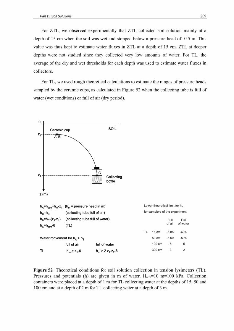
Part D: Soil Solutions 209
For ZTL, we observed experimentally that ZTL collected soil solution mainly at a
depth of 15 cm when the soil was wet and stopped below a pressure head of -0.5 m. This
value was thus kept to estimate water fluxes in ZTL at a depth of 15 cm. ZTL at deeper
depths were not studied since they collected very low amounts of water. For TL, the
average of the dry and wet thresholds for each depth was used to estimate water fluxes in
collectors.
For TL, we used rough theoretical calculations to estimate the ranges of pressure heads
sampled by the ceramic cups, as calculated in Figure 52 when the collecting tube is full of
water (wet conditions) or full of air (dry period).
SOIL
z (m)
0
z1
z2
Ceramic cup
Collectingbottle
A B
C
hA=hatm+hm-z1 (hm = pressure head in m)
hB=hC (collecting tube full of air)
hB=hC-(z2-z1) (collecting tube full of water)
hC=hatm-6 (TL)
Water movement for hA > hB
full of air full of water
TL hm > z1-6 hm > 2 z1-z2-6
SOIL
z (m)
0
z1
z2
Ceramic cup
Collectingbottle
A B
C
hA=hatm+hm-z1 (hm = pressure head in m)
hB=hC (collecting tube full of air)
hB=hC-(z2-z1) (collecting tube full of water)
hC=hatm-6 (TL)
Water movement for hA > hB
full of air full of water
TL hm > z1-6 hm > 2 z1-z2-6
Lower theoretical limit for hm
for samplers of the experiment
Full of air
Full of water
TL 15 cm -5.85 -6.30
50 cm -5.50 -5.50
100 cm -5 -5
300 cm -3 -2
Figure 52 Theoretical conditions for soil solution collection in tension lysimeters (TL). Pressures and potentials (h) are given in m of water. Hatm=10 m=100 kPa. Collection containers were placed at a depth of 1 m for TL collecting water at the depths of 15, 50 and 100 cm and at a depth of 2 m for TL collecting water at a depth of 3 m.

Part D: Soil Solutions 210
The ceramic cups were considered as ideal and punctual samplers. Actually, the
samplers are not ideals (porosity and wettability of ceramic cups, dimension of the
collecting pipe…) and the collection tubes are neither full of air nor full water but
generally constituted of a succession of complex biphasic water / gaz bubble systems. The
calculated ranges of pressure for ZTL used for further calculations are thus theoretical and
may differ from the ranges of pressure truly collected in the field.
Only drainage fluxes were taken into account since it was impossible to differentiate
soil solution due to upward fluxes from soil solution due to downward fluxes in the
solutions collected by the lysimeters.
D.1.2.2.2 Calculation of nutrient fluxes
Nutrient fluxes were obtained by multiplying the nutrient concentration measured in the
soil solution by the water flux estimated from the above paragraph for the collecting
lysimeter.
As already mentioned in the water fluxes section, the water flux was considered
invariant in the horizontal plane. For a given observation date and depth, the differences
between two nutrient fluxes in two different treatments, blocks, or collectors, were thus the
result of differences in the nutrient concentrations.
D.1.2.3 Missing data and aberrant data tracking
Missing data occurred when (i) no water was collected by the collecting device because the
pressure head was below the pressure head threshold of the device, or for TL in case of
vacuum drop, (ii) the collected volume was insufficient to perform chemical analyses, (iii)
the analysis was missing (hardly ever).
Missing data are classically estimated from other collectors and sampling times. This
was not performed here since the fertilization events resulted in localized (time and space)
very high peaks of concentration, and since there were few records left uninfluenced by
these events (management practices). Missing data were thus considered as “not a number”
(NaN) for concentrations and nutrient fluxes (integrated as spatial heterogeneity). Average
fluxes were always calculated from an average concentration multiplied by the water flux
so that an average flux was null only when all fluxes composing the average were null.

Part D: Soil Solutions 211
For the same reasons than for missing analysis, no efficient aberrant data tracking
could be reliably performed. For a given sample, it was impossible to differentiate sample
pollution during the analytical process from a fertilization peak. Ionic balances were
checked but pollution often occurs as a cation-anion pair. Moreover, organic charges (DOC
and DON) contributed quite largely to the ionic balance for some samples but their charge
could not be determined. The analytical process was carefully checked. Data were kept un-
modified and the analytical risk of pollution was integrated as spatial variability.
D.1.2.4 Analysis of the concentrations and cumulative fluxes signals
D.1.2.4.1 General strategy
The time-course of concentrations and cumulative fluxes can be analyzed as spectra (same
as a chromatogram spectrum for concentrations and same as a pH-titration for cumulative
fluxes). In this study, an equivalent chromatogram was considered constituted of three
parts: the baseline, the background signal, and the exceptional events:
• the baseline contains the analysis uncertainty and the average minimum signal,
• the background signal (above the baseline) reflects the mean specific signal of the
ecosystem without exceptional perturbations, spatial variability among collectors
and analysis uncertainty,
• and the exceptional events (major peaks) represent flushes of nutrients in solutions
due to specific processes (high atmospheric deposits, fertilization, microbial
activity …).
Baseline and background signals depend on collector type, collection depth and mineral
element analyzed. Exceptional events depend mainly on changes in the entry signal
(rainfall) and on silvicultural practices. The main difficulty in such an analysis is to define
the baseline, the ecosystem background signal and the threshold above which a peak is
regarded exceptional.
D.1.2.4.2 Baseline, background signal and thresholds
Our main goal was to study the exceptional events, that is, the clear felling and the
fertilization effects. Usually, the baseline and background signals are estimated from a
time-period poor in exceptional event and long enough to include seasonal variations.

Part D: Soil Solutions 212
Consequently, the exceptional events are those concentration peaks greater than the
average variations around the background signal. Our study period was too short to do so,
particularly for tension lysimeters for which almost no data were available before clear
felling.
The baseline was thus estimated from concentration spectra for each mineral element,
as the first quartile of all measured data (3 blocks x 3 treatments x 37 months) for each
collector type and depth. The first quartile was chosen since it favors the lower values and
minimizes the effect of exceptional events on the result. This baseline was subtracted to
cumulative fluxes to better analyze the effect of exceptional events on the nutrient flux
dynamics.
Background signal was defined only for aboveground collectors (for which few
exceptional events occurred) as the median of the population for each collector type and
mineral element analyzed.
The threshold for exceptional events was not calculated from the background signal
but from the maximum signal resulting from exceptional events (CFmax). This maximum
was calculated as the maximum of all final (Nmonth=37) cumulative fluxes after baseline
subtraction (average per treatment, collector type and collection depth). The average
cumulative flux was chosen for minimizing the influence of localized (time and space)
large concentration peaks and for integrating the whole period of the experiment. CFmax
was taken as the maximum for all collector types, collecting depths, treatments and mineral
elements (expressed in mmol) in order to have a common reference for all collectors, that
is, (i) to identify the maximum response of the ecosystem to a given perturbation, (ii) to
observe its attenuation with depth and its dispersion in time and space, and (iii) to compare
its intensity according to the mineral element observed. For DOC which could not be
expressed in mmol, CFmax was taken as the greatest cumulative flux recorded.
The threshold above which a final cumulative flux is considered to have experienced
an exceptional event (CFt) was then taken as CFt=CFmax/50, which is approximately one
tenth of the CFmax transmitted at a depth of 3 m given the attenuation of the water flux at
this depth. The threshold for nutrient fluxes CF’t was taken as CF’t=CFt/12, where CFt/12
represents the average monthly ionic flux of CFt spread over 12 months (actually observed
for the present study). The threshold for concentrations (Ct) was then CF’t divided by the
average monthly water flux.

Part D: Soil Solutions 213
D.1.2.4.3 Spectra analysis
0 5 10 15 20 25 30 35 40
0
0.5
1
Co
nce
ntr
atio
n (
mm
ol)
0 370
0.51
Nmonth
C
0 1 2 3 4 5 6 7 8 9 100
0.51
1.5BaselineBackground ecosystem signalBaseline + threshold for exceptional events
Average dataSplineSpline 1st derivative
Figure 53 Example of spectrum analysis for concentrations.
0 5 10 15 20 25 30 35 40
0
250
500
∨
∧
32%
∨
∧
52%
max=100%
Cu
mu
lati
ve f
lux
- B
asel
ine
(mm
ol)
0 370
0.51
32 52
Nmonth
C
0 1 2 3 4 5 6 7 8 9 100
0.51
1.5Average dataThreshold
Spline modelizing the averageSpline: 1st derivativeSpline: 2nd derivative
Figure 54 Example of spectrum analysis for cumulative flux.

Part D: Soil Solutions 214
Spectra analysis had to be performed on a continuous function whereas experimental
data were discontinuous at a monthly time step. The concentration spectra were thus
simulated continuously thanks to a slightly smoothed spline using Matlab software
(www.mathworks.fr). The peaks of the spectra were then calculated as the zeros of the
spline 1st derivative for which the concentration was above baseline+Ct ( Figure 53).
For cumulative fluxes, only the spectra for which the final cumulative flux was above
CFt were analyzed. The data were also simulated thanks to a slightly smoothed spline. The
equivalences between two plateaus (time and intensity) were given by the zero of the
second derivative of the spline ( Figure 54).
The concentration spectra were mainly used qualitatively to localize exceptional events
and to compare the dynamics of one nutrient in respect to the others. Cumulative fluxes
were used for all quantitative studies.
D.1.2.5 Ionic strength
The ionic strength (IS) in mol was calculated as:
212 i i
iIS z C= ∑ (58)
where i are the mineral elements in solution, zi is the charge of each element and Ci its
concentration in mol L-1. The charge attributed to each element was +1 for K, Na and NH4,
+2 for Ca and Mg, +3 for Al and Fe, -1 for Cl, NO2, NO3 and H2PO4, and -2 for SO4.
Ionic strength was calculated as an indicator of the status of the sampled solution but
since no speciation study was performed (especially for Al), it must be handled cautiously.
The pKe of the first acidity of Al is 5 (Stumm and Morgan, 1996) and soil solution pH
were mainly < 5 so that Al was considered as 3+ in the ionic strength calculation. It is
obviously a rough approximation since organic ligands and locally basic pH may reduce
the positive charge of Al (Driscoll and Schecher, 1990).
D.1.2.6 Statistical analyses
The effect of treatment on cumulative fluxes (from the clear felling until the end of the
experimental period) was tested for each collector type and depth, and for each element
thanks to one-way ANOVA analyses and t-tests using proc GLM of SAS Software.
Differences among treatments were considered significant at P < 0.05.

Part D: Soil Solutions 215
D.1.2.7 Sequence of data analysis adopted
Finally the data analysis was performed in the following way:
• All mass data were converted to moles to enable direct comparisons among
elements.
• Baselines and thresholds were first calculated on concentration spectra and
cumulative flux spectra respectively.
• Aboveground fluxes were studied mainly on the basis of their concentration
spectra. Baseline and background signal (median) were quantified and exceptional
events localized to identify whether atmospheric events may interfere with clear
felling and fertilization events in soil solution signals.
• Soil solutions were then studied considering ZTL only at a depth of 15 cm (since
deeper ZTL collected almost no water), and TL only after February 2004 (since
vacuum difficulties did not allow continuous sampling before). Cumulative fluxes
were studied, once their baseline subtracted, for the whole period continuously so
that, unless mentioned, an offset must be considered between ZTL and TL. It was
done so in order to better visualize the ecosystem background signal from
exceptional events when those signals were both available (ZTL).
• Nitrate and sulphate were analyzed in detail as case studies. For these two
elements, the average concentration and the average cumulative flux spectra were
first studied for each collector type, collection depth and treatment. The spatial
variability of the signal among the three blocks was studied qualitatively reporting
the data of each block on the studied average spectra. The spatial variability
among individual collectors was also studied on cumulative fluxes by qualitatively
comparing the spectrum analysis of each individual collector (available for TL at
depths 50 cm, 100 cm and 300 cm in treatments 3 and 5). Concentrations in
solutions collected by ZTL and TL were qualitatively compared at a depth of 15
cm.
• Differences in nutrient dynamics were finally studied by comparing the average
spectra analysis for each nutrient (concentrations and cumulative fluxes). Total
cumulative fluxes (including baseline) from the clear felling to the end of the

Part D: Soil Solutions 216
experiment (no more offset between ZTL and TL) were finally given with their
standard errors (variability among blocks and collectors).
To better visualize the differences among collectors or elements, the projections of the
concentration and cumulative spectras on the time axis were generally preferred to their
corresponding 2D-plots which are space consuming ( Figure 53 & Figure 54).

Part D: Soil Solutions 217
D.2 RESULTS AND DISCUSSION
D.2.1 Water fluxes collected by the lysimeters calculated from the
MIN3P simulations
0
1000
2000
3000
4000
7 8 9 10 11 12 12.
12.
2 3 4 5 6 7 8 9 10 11 12 12.
12.
2 3 4 5 6 7 8 9 10 11 12 12.
12.
2 3 4
2003 2004 2005 2006
Wat
er c
umul
ativ
e flu
x (m
m)
Rainfall
ZTL 15 cmTL 15 cmTL 50 cm
TL 100 cmTL 300 cmTotal 300 cm
Figure 55 Estimated cumulative water fluxes (mm) drained in the soil profile (total) and collected by the lysimeters (ZTL=zero-tension lysimeter, TL= tension lysimeter) at a given depth (estimation from the water flux model of part C and from the pressure head ranges of D.1.2.2). The cumulative flux measured for rainfall is also represented.
0
50
100
150
200
250
300
7 8 9 10 11 12 1 2.1 2.2 3 4 5 6 7 8 9 10 11 12 1 2.1 2.2 3 4 5 6 7 8 9 10 11 12 1 2.1 2.2 3 4
2003 2004 2005 2006
Wat
er fl
ux (m
m)
Rainfall TL - 15 cm TL - 300 cm
t=2-3
t=15-16 t=28-29
t=34-37
t=21
t=5-8
Figure 56 Water fluxes (mm) measured for rainfall (Pi) and calculated from the soil water flux model for tension lysimeters (TL) at the depths of 15 cm and 300 cm, over the studied period. The most pronounced wet and drought events are indicated in total months elapsed since the beginning of the study (t=Nmonth).

Part D: Soil Solutions 218
At the depths of 15 cm, 50 cm and 150 cm, the calculations show that tension lysimeters
may collect the whole soil water flux simulated by the water drainage module of MIN3P
(part C). Indeed, the pressure head theoretically collected by TL at these depths ranged
from less than -5 m to 0 m ( Table 37) which corresponded to the whole retention curve of
Figure 39, that is, to the entire water flux simulated at these depths. As the lower boundary
-5 m is located on a plateau of the retention curve, a slight change in this lower boundary
will not influence much the water flux collected. These calculations were confirmed by
field observations: TL always collected water at these depths during the periods of
drainage indicated by the model. TL water fluxes thus calculated are likely to approximate
the water fluxes effectively collected at these depths as far as (i) the water flux model is
accurate, (ii) TL do not deviate too much from their ideal behavior, and (iii) a constant
vacuum is guaranteed.
At a depth of 300 cm, calculations show that TL may collect the whole soil water flux
when the soil is wet but barely any flux during the very dry period of February 2006.
Indeed, the pressure head theoretically collected by TL at a depth of 3 m ranged from
about -2.5 m to 0 m. The lower boundary -2.5 m is located on the far end of the steep
decreasing part of the retention curve which meant that (i) the collected water flux
represents almost the whole water flux except a residual part moving very slowly in the
soil profile, and (ii) a small change or error of determination in the lower boundary may
influence greatly the water flux fraction collected. These calculations were confirmed on
field: TL at a depth of 300 cm showed a greater heterogeneity in their ability to collect
water during the dry periods and were very sensitive to slight drops of the vacuum applied.
The model used to compute the water flux collected in TL at a depth of 300 cm is thus
submitted to the same restrictions as mentioned for TL at depths of 15, 50 and 150 cm, and
is likely to overestimate the water flux effectively collected during the dry periods. As a
direct consequence, TL at a depth of 300 cm may not sample the whole soil water flux
during the dry periods.
The model estimated that the proportion of the whole drainage sampled by ZTL was in
average 80% at a depth of 15 cm ( Figure 55 & Figure 56) which, once more, corresponded
to the steep part of the retention curves of Figure 39. This means that ZTL are expected to
collect the major part of the water collected by TL at a depth of 15 cm especially in periods
of large drainage (high pressure heads). On the other hand, the solutions collected by TL
and ZTL are expected to differ when drainage occurs at lower pressure heads. Moreover,

Part D: Soil Solutions 219
as TL collect water down to lower pressure heads, TL may collect chemical species in a
lower state of potential than does ZTL, that is, species moving in soil solution closer to the
soil surface than does ZTL (due to specific adsorption or in smaller pores for example).
The fact that almost no water was collected in ZTL at the depths of 50 cm and 100 cm
confirms that no major preferential flow occurred in the studied soils. As mentioned in
section 5 (water flux model), intensive water drainage occurred down to a depth of 3 m
from November 2003 to February 1 2004 (Nmonth=5 to 8), in February 1 2005 (Nmonth=21),
and from February 1 to March 2006 (Nmonth=34 to 37). Periods of drought occurred in
August and September of each year (Nmonth=2-3, 15-16, and 28-29). At a depth of 300 cm,
the 2005-2006 drought lasted from 07/2005 until 02-2/2006.

Part D: Soil Solutions 220
D.2.2 Median and quartile, aboveground solutions
D.2.2.1 Baselines
Table 38 Concentration baselines (μmol L-1 and mg L-1 for DOC) calculated for each element and collector type as the 1st quartile of all blocks and treatments data for the studied period and background ecosystem signal calculated for aboveground collector as the medians of all blocks and treatments data.
Element concentration H Cl NO2 SO4 NO3 H2PO4 Na NH4 K Mg Ca Fe Al Si DOC
Collector type
Depth (cm)
μmol L-1 mg L-1
1st quartile = baseline
Aboveground and stream collectors S 1 9 0 0 17 0 3 11 10 1 170 1Pi 2 9 3 7 4 4 3 2 6 1 1Th 3 13 3 7 6 5 10 4 7 0 2St 7 32
0
3 5
0
23 2 26 10 14 0
0
0 15
Soil and forest floor solution collectors ZTL 0 2 33 5 7 17 3 30 23 29 2 6 7 19
15 43 30 7 9 15 1 8 16 10 1 11 33 8TL 15 25 37 6 7 18 0 8 15 15 19 121 4
50 28 34 1 16 14 1 6 8 13 23 129 2 100 28 35 0 44 13 0 3 6 8 17 99 1 300 4 10
0
0 26
0
10 0 3 4 9
0
0 80 1
Median = ecosystem background
Aboveground and stream collectors S 2 15 0 0 0 19 0 5 15 15 2 1 190 2Pi 4 11 1 5 12 6 16 6 4 9 0 1 1Th 5 20 1 6 14 10 10 14 7 13 0 1 4St 16 48 0 4 9
0
42 9 43 21 28 0
1 1 26
S=Stream, Pi=rainfall, Th=Throughfall, St=Stemflow, ZTL=zero tension lysimeter, TL=tension lysimeter
All baselines except Si (< 170 μmol L-1) and DOC (DOC < 19 mg L-1) were < 50 μmol L-1
( Table 38). For NO2, PO4 and Fe the baselines and medians were very low (< 2 μmol L-1)
whatever the collector. The analytical “noise” was thus generally < 0.5 ppm whatever the
element analyzed so that the concentrations above this threshold can be reliably attributed
to the ecosystem. It also indicates that no major continuous pollution occurred for all the
collecting devices.
Al and Si baselines were respectively 2 and 4 times as much in TL as in ZTL at a
depth of 15 cm. This behavior could be explained by the influence of the high
concentration peaks occurring after clear felling and fertilizing on the baseline calculation
for TL (contrary to ZTL, no before-clear-felling data were used to calculate TL baseline),

Part D: Soil Solutions 221
or to a slight contamination of the soil extracts by the porous cup material as classically
observed (Titus and Mahendrappa, 1996). In contrast, H and DOC baselines were two
times as much in ZTL as in TL. The filtration of large organic molecules through the poral
network of the ceramic cups (TL) is also classically observed (Corwin, 2002; Titus and
Mahendrappa, 1996).
Stream baselines (but Si) were < 20 μmol L-1 and equaled 1 mg L-1 for DOC. The
ecosystem background was less than two times its corresponding baseline. This average
signal is far less than the legislation of drinkable water of the European Union for all
elements (UE, 1998) and indicates high quality water regarding the measured elements.
Aboveground solutions contained very small amounts of NO2, H2PO4, Fe, Al and Si
(baselines and medians < 2 μmol L-1). The stemflow ecosystem background was about
twice the throughfall one, and four times the rainfall one for Cl, K, Mg and Ca (rainfall
medians of 5 μmol L-1 for Mg, 6 μmol L-1 for Na and K, 9 μmol L-1 for Ca and of 11 μmol
L-1 for Cl). SO4 ecosystem background was more or less the same for all collectors (median
of about 6 μmol L-1). H and DOC ecosystem backgrounds were low in rainfall and
throughfall (medians < 5 μmol L-1 and mg L-1) but increased in stemflow (medians of 16
μmol L-1 for H and 26 mg L-1 for DOC). The opposite behaviour was observed for NO3
(medians of about 13 μmol L-1 in rainfall and throughfall, and of 9 μmol L-1 in stemflow)
and NH4 (medians of 16, 10 and 9 μmol L-1 in rainfall, throughfall and stemflow
respectively). The baseline pH decreased in the following order: stream (5.7) > Rainfall
(5.4) > Throughfall (5.3) > Stemflow (4.8). The ecosystem backgrounds ranged between
once to twice their corresponding baselines.
The overall pattern for above ground solutions is thus that an increase in H, Cl, K, Mg,
Ca and DOC occurs while passing through the Eucalyptus crown (throughfall) or when
running off the Eucalyptus stem. On the contrary, uptake of nitrogen through its nitrate or
ammoniacal form occurred during the transfer of the solution from the canopy to the soil.
This pattern is classically observed in tropical forests (Xu et al., 2005) and plantations
(Laclau et al., 2003a) as well as in temperate forests on N deficient soils (Gonzalez-Arias
et al., 2006; Klopatek et al., 2006). Stemflow do not represent much of the water flux
entering the soil, but as its input is localized at the stem basis and its solutions are
particularly concentrated, they may induce a heterogeneous pattern in soil solutions along
main roots (Beier, 1998; Cattan et al., 2007; Levia and Frost, 2003).

Part D: Soil Solutions 222
The corresponding baselines in term of cumulative fluxes are given in Table 39.
D.2.2.2 Thresholds
Table 39 Baseline cumulative flux (mmol L-1 and mg L-1 for DOC) for each element, collector type and collection depth (all blocks and treatments taken altogether for the studied period), and cumulative flux minus baseline cumulative flux for each element, collector type, collection depth and treatment (all blocks taken altogether for the studied period). The maximum cumulative flux is given in bold.
Element cumulative flux over the 37 months of the studied period H Cl NO2 SO4 NO3 PO4 Na NH4 K Mg Ca Fe Al Si DOCCollector
type Depth (cm) Tr
mmol g
Baseline cumulative flux Pi 8 36 1 12 28 0 17 17 14 9 26 0 0 2 4
ZTL 0 7 129 0 19 27 0 66 12 115 90 113 9 24 25 72 15 112 78 0 18 24 0 38 2 21 40 27 3 29 87 21
TL 15 55 80 0 13 16 0 39 0 18 32 33 0 42 264 9 50 54 66 0 2 31 0 28 1 11 17 26 0 45 254 5 100 48 61 0 0 76 0 22 0 6 10 15 0 29 172 2 300
Ave
rage
4 10 0 0 26 0 10 0 3 4 9 0 0 80 1
Cumulative flux – Baseline cumulative flux Pi 22 36 3 6 20 1 12 41 8 6 9 0 0 6 2
ZTL 0 1 58 149 15 9 37 2 39 43 97 168 88 1 2 10 25 3 91 249 13 196 36 7 78 376 156 159 98 8 11 13 37 5 118 257 17 218 84 10 103 346 155 18 53 24 18 22 25 15 1 104 70 2 4 181 1 32 25 32 24 17 1 43 27 8 3 193 151 6 303 254 19 71 187 86 65 75 1 79 54 15 5 244 227 7 276 588 1 40 364 83 29 80 2 240 94 6
TL 15 1 30 275 4 29 325 1 120 20 90 49 34 0 69 53 6 3 63 80 3 320 456 96 119 131 63 94 235 0 108 66 9 5 78 323 5 75 572 3 54 28 191 19 37 0 189 12 2 50 1 35 335 1 11 328 0 139 104 101 23 8 0 109 9 3 3 23 99 2 83 428 2 109 94 46 39 45 0 102 11 4 5 46 300 2 6 624 0 54 8 200 17 10 0 203 65 1 100 1 32 592 1 2 211 0 78 97 211 17 15 0 130 54 3 3 1 70 1 3 316 0 146 53 21 21 17 0 51 0 3 5 32 105 5 1 355 0 51 5 35 16 15 0 130 0 2 300 1 5 8 0 0 16 0 12 5 2 6 12 0 15 15 3 3 2 2 1 0 3 0 4 4 1 1 1 0 1 0 1 5 11 6 0 0 22 0 34 4 1 3 7 0 3 0 1
Maxima 244 592 17 320 624 96 146 376 211 168 235 24 240 94 37
As mentioned in the material and methods sections, the thresholds were calculated from
the cumulative flux for each element, treatment, collector type and collection depth, once
the baseline subtracted ( Table 39). The greatest cumulative flux (624 mmol) was obtained

Part D: Soil Solutions 223
for nitrate, in TL of treatment 3 at a depth of 50 cm. The threshold for cumulative fluxes
was then of SCt=12.5 mmol (734 mg for DOC), which was of the same order of magnitude
than Pi cumulative fluxes. The threshold for ion flux was then SC’t=1.04 mmol month-1 (61
mg month-1 for DOC). The average water flux for TL at 50 cm was of 66 mm month-1,
which gave a threshold for concentrations of Ct=16 μmol L-1 (1 mg L-1 for DOC).
ANOVA analysis were not performed for the data of Table 39 since such an analysis
will be finally performed on cumulative fluxes from the clear felling until the end of the
experimental period to conclude the soil solution chapter in § D.2.5.4.
D.2.2.3 Exceptional events for aboveground solutions
0 10 20 30 400
0.1
0.2
0.3
NO
3 co
nce
ntr
atio
n (
mm
ol L
-1)
Pi
↓t=3
↓t=15-16
↓t=28
Date (month)0 10 20 30 40
0
0.1
0.2
0.3
↓t=3
St
Date (month)0 10 20 30 40
0
0.1
0.2
0.3
↓t=3 ↓
t=28
Th
Date (month)
measured concentration median quartile threshold spline
Figure 57 Time-course (t=Nmonth) of nitrate concentrations (mmol L-1) in aboveground collectors (Pi=Rainfall, Th=Throughfall, St=Stemflow). The first quartile (baseline) and the medians (ecosystem background) of the populations are given, together with the concentration threshold (Ct=16 μmol L-1) and the spline modelizing the average.
Aboveground solution concentrations were homogeneously dispersed around the median
concentration ( Figure 57 for nitrates). Baselines and medians were below Ct except for Cl,
Na, K, Mg and Ca in stemflow collectors which were in the range [threshold, threshold*3].
Once more, it is suggested that even if stemflows represent a small part of the total inflow
at the upper boundary of the soil profile it can induce patterns of spatial heterogeneities in
nutrients fluxes (Beier, 1998; Cattan et al., 2007; Levia and Frost, 2003).

Part D: Soil Solutions 224
Table 40 Time (t=Nmonth) and intensity (mmol L-1) of exceptional events in aboveground solutions collectors (Pi=Rainfall, Th=Throughfall, St=Stemflow).
H Cl NO2 SO4 NO3 PO4 Na NH4 K Mg Ca Fe Al Si DOC Nmonth
Collector type mmol L-1 mg L-1
3 Pi - - - - 0.03 - - 0.05 - - 0.04 - - - 2.94 St - - - - 0.05 - 0.55 0.07 0.26 0.19 0.22 - - - - Th - - - 0.03 0.04 - 0.03 0.05 0.04 0.02 0.05 - - - 6.21
15-16 Pi - 0.19 - 0.08 0.29 - 0.07 0.19 0.09 0.09 0.15 - - - 22.11
28 Pi - 0.04 - - 0.05 - - 0.07 0.02 - 0.03 - - - 3.93 Th - 0.12 - 0.02 0.05 - 0.03 0.05 0.06 0.04 0.06 - - - 12.21
The concentration spectra analysis for aboveground collectors outlined three events
above Ct for Nmonth=3, 15-16, and 28 ( Table 40 and Figure 57) for all elements but Fe, Al,
Si, H, NO2 and PO4 which were always very low for aboveground collectors. The main
peak occurred at Nmonth=15-16 for which rainfall concentrations reached 0.29 mmol L-1 for
NO3, 0.19 mmol L-1 for Cl and NH4, 0.15 mmol L-1 for Ca and 22.11 mg L-1 for DOC.
Exceptional events could not be seen in stemflow at Nmonth=15-16 and Nmonth=28, and in
throughfall at Nmonth=15-16, since these collectors were disabled at these dates. These three
concentration peaks corresponded to the dryer months of years 2003, 2004 and 2005
during which rainfall was < 30 mm month-1. They may be attributed to the leaching by
small amounts of water of dry depositions accumulated during the droughts, as classically
observed (Laclau et al., 2003a).
As a conclusion, the large concentrations which may be observed in the forest floor
and soil solutions may not result from the average input of throughfall. Concentration
peaks up to 0.05 mmol L-1 may locally (at the stem basis) result from the average stemflow
input. Concentration peaks up to 0.3 mmol L-1 may result from exceptionally concentrated
stemflow and throughfall inputs during the dry periods. Figure 58 summaries the
chronology of events related to high concentrations in aboveground collectors or to the
ecosystem management.

Part D: Soil Solutions 225
0 10 20 30 40
0 37Nmonth→
Drought
AGpeak
↓
2-3
Drought
AGpeak
↓
15-16
Drought
AGpeak
↓
28-29
Wet
↓ ↓
5-8
Wet
↓
21
Wet
↓ ↓
34-37
Clear Felling
↑
9
Planting
Fertilisations
[1]
↑
11
[2]
↑
19-20
[3]
↑
25
[4]
↑
31
7 8 9 10 11 12 12.
12.
2 3 4 5 6 7 8 9 10 11 12 12.
12.
2 3 4 5 6 7 8 9 10 11 12 12.
12.
2 3 4
2003 2004 2005 2006
↓↓↓↓ ↓ ↓ ↓↓↓ ↓↓ ↓ ↓
Figure 58 Chronology of events related to high concentrations in aboveground collectors (AGpeak), to the weather (wet or drought) or to the ecosystem management (mainly silviculture) in the experiment.
D.2.3 Soil solutions, case study 1: nitrate
D.2.3.1 Concentrations

Part D: Soil Solutions 226
Figure 59 Time course of the concentration in nitrate (mmol L-1) measured in each treatment and soil solution collector (ZTL=zero tension lysimeter, TL=Tension lysimeter) over the 37 months of monitoring. The quartile and median of the populations (all treatments taken altogether) are represented. The main peaks localized above the threshold of § D.2.2.2 are indicated together with the spline modelizing the average concentration.

Part D: Soil Solutions 227
Forest floor solutions showed a nitrate concentration peak in T3 and T5 at Nmonth=15-16
(Clear Felling (CF) + 6 months), which corresponded to a drought period and consequently
to a nitrate concentration peak in solutions collected above ground ( Figure 59).
0 10 20 30 400
1
2
[NO
3] (m
mo
l L-1
)
Date (month)
T1
0 10 20 30 400
1
2
Date (month)
T3
0 10 20 30 400
1
2
T5
Date (month)
0 1 2 3 4 5 6 7 8 9 10-1
0
1
Measured data ZTL Measured data TL Spline ZTL Spline TL
Figure 60 Nitrate concentrations in mmol L-1 measured in zero tension lysimeter (ZTL) and tension lysimeter (TL) at a depth of 15 cm. The spline modelizing the average concentration is also represented.
At a depth of 15 cm, the dynamics of nitrate concentrations were equivalent in ZTL
and TL ( Figure 60) as was suggested by the water fluxes study (§ D.2.1). Three major
concentration peaks occurred in T1 at Nmonth=12 (CF+2), Nmonth=15-16 (CF+5, drought and
AG peak), and Nmonth=19 (CF+10, Fertilisation 2 with KCl (F2)). Concentrations peaks
were greater in T3 and T5 than in T1 so that one single peak at Nmonth=13-14 (CF+4) could
be distinguished.
The concentration peaks were transmitted at a depth of 50 cm at Nmonth=14-15 (CF+5),
18-19 (CF+9) and 27 (CF+18, F2+8). The delay between concentration peaks at 15 cm and
at 50 cm ranged from 3-4 months to 8 months in case of drought periods.
At a depth of 100 cm, the concentration peaks appeared at Nmonth=15 (CF+6), 21-23
(CF+12, large drainage period after drought) and Nmonth=30 (CF+21, F2+11, large drainage
period after drought). The delay between concentration peaks at 50 cm and at 100 cm was
thus of about 3 months.
At a depth of 300 cm, no significantly large nitrate peak was observed.

Part D: Soil Solutions 228
NO3 concentrations reached up to 3, 1.5, 1 and < 0.2 mmol L-1 at the depths of 15, 50,
150 and 300 cm respectively, which corresponded to 217, 93, 62, and 12 mg L-1
respectively.
The projection of each plot of Figure 60 on the time axis informs more in detail on the
onset and ends of the peaks ( Figure 61).
0 10 20 30 40
Clear Felling
ZTL0 cm T1T3 0.2
T5 0.2
15 cm T1 0.8 0.3
T3 1.2
T5 2.3
TL 15 cm T1 0.6 0.6 0.5
T3 1.3
T5 1.3
50 cm T1 0.8 0.5
T3 0.8 1 0.2 0.3
T5 0.5 0.8 1.2 0.3
100 cmT1 0.5
T3 0.8 0.2 0.2
T5 0.7 0.8
300 cmT1T3T5
NO3
Date (month)
0 15
0
0.5
[NO
3- ]
max
Date (month)
Legend
0 10 200
5
10
~
max
max
if max < 0.16 mmol L-1
if max < 0.32 mmol L-1
if max > 0.32 mmol L-1
↑ ↑
Figure 61 Projection of the average concentration in nitrate (mmol L-1) measured in each treatment (T1, T3 and T5) and soil solution collector (ZTL=zero tension lysimeter, TL=Tension lysimeter) on the time axis (month). Only concentration peaks above the threshold Ct are represented. The value of 0.16 mmol L-1 was chosen as ten times the threshold defined for concentrations (§ D.1.2.4.2).
Figure 61 confirms that all peaks were weak in the forest floor solutions. They
occurred after droughts (Nmonth=3, 16-19, 30-31), high rainy events (Nmonth=22) and after N
fertilizer was spread on soil (Nmonth=12 (F1) in T5 and 19-22 (F2) in T3 and T5). The main
peak started at Nmonth=14 (CF+5) in all treatments and lasted 3 months in T1, 4 months in
T3 and 5 months in T5.
The main concentration peak started at clear felling (Nmonth=9) at a depth of 15 cm (TL
and ZTL) and at 50 cm. At a depth of 100 cm, it started weakly at Nmonth=11 (CF+2) then

Part D: Soil Solutions 229
markedly at Nmonth=17 (CF+8, first large drainage period after drought). At a depth of 300
cm, concentration peaks appeared very weakly (max<0.16 mmol L-1).
Main peaks lasted longer in T5 (16 months at 15 cm, 21 months at 50 cm and 17
months at 100 cm) than in T3 (13 months at 15 cm, 19 months at 50 cm and 16 months at
100 cm) and in T1 (13 months at 15 cm, 14 months at 50 cm and 11 months at 100 cm).
Greatest peak intensities were always observed in T3 or T5.

Part D: Soil Solutions 230
D.2.3.2 Cumulative fluxes
Figure 62 Cumulative fluxes (minus baseline) of nitrates (mmol) calculated for each soil solution collector (ZTL=zero-tension lysimeter, TL=tension lysimeter) in each treatment (T1, T3 & T5) over the 37 months of the studied period. The threshold for cumulative fluxes SCt is represented, together with the spline modelizing the average cumulative flux for all blocks (n=3). The main steps are indicated.

Part D: Soil Solutions 231
Events appear far more homogeneously for cumulative nitrate fluxes than for
concentrations. Four nitrate flushes occurred at Nmonth=4 (after 1st drought) in ZTL at 15
cm, Nmonth=10-11 (CFP period) and Nmonth=17-21 (F2, intensive drainage period after
drought) for all collectors and depths, and Nmonth=30-32 (F4, intensive drainage period
after drought) in the forest floor.
0 10 20 30 40
Clear Felling
ZTL 0 cm T1 370.59 41 29
T3 360.337 38
T5 840.515 48 14
15 cm T1 181NaN1 42 36
T3 2540.61 43 36
T5 5882.50 31 46
TL 15 cm T1 325-0.225 58
T3 4560.132 52
T5 5721.919 57
50 cm T1 328-0.618 62
T3 4282.116 63
T5 6242.37 70
100 cm T1 2110.55 72
T3 3161.31 75
T5 3552.70 77
300 cm T1 160.124 50
T3 30.2
T5 22NaN27 53
NO3
Date (month)
tan(α) max(mmol)
0 15
0
1
↑
↓
Δ
_ _ _αC
Cum
. Flu
x (m
mol
)
max
Date (month)
Legend
0 10 200
5
10
~
h(%) = 100 Δ/max
h(%)
h(%)
h(%) if h(%) < 10
if h(%) < 30
if h(%) > 30
↑ ↑
Figure 63 Projection of the average cumulative nitrate fluxes (mmol) (minus baseline) calculated for each soil solution collector (ZTL=zero-tension lysimeter, TL=tension lysimeter) in each treatment (T1, T3 & T5) on the time axis (month). The cumulative flux (max) and the slope of the curve tangent (tan α) at the end of the experimental period are indicated. The contribution of each step to the final cumulative flux is also given (h(%)). Steps were calculated only when max > SCt (§ D.2.2.2). NaN stands for non calculable (tangent close to zero or step still running at the end of the studied period).
The projection of the average cumulative nitrate fluxes on the time axis ( Figure 63)
shows that the flushes last in average four months. At a depth of 15 cm, two concentration
flushes contribute to final cumulative fluxes in equal proportion for ZTL (40 % each). In
TL, whilst the contribution of the 1st flush decreases with depth (30% at 15 cm, 20% at 50
cm and less than 5% at 100 cm), the contribution of the second flush increases (55% at 15
cm, 65% at 50 cm and 75 % at 100 cm).

Part D: Soil Solutions 232
Final cumulative fluxes were very small at a depth of 300 cm (< 21 mmol). They were
always in the following order: T5 > T3 > T1. Quasi no attenuation of the total nitrate flux
was observed between TL at 15 cm and TL at 50 cm (max≈325 mmol in T1, max≈440
mmol in T3, max≈500 mmol in T5). About 2/3 of the 15 and 50 cm fluxes reached a depth
of 100 cm (max=211 mmol in T1, max=316 mmol in T3, max=355 mmol in T5). In the
forest floor, cumulated fluxes over the whole period were about 10 % of the fluxes
estimated from TL collectors (max=37 mmol in T1 and T3, max=84 mmol in T5).
The slope of the curve tangent at the end of the experiment (tanα) showed that a
plateau was reached in T1 and T3 at the depths of 0 cm and 15 cm (tanα close to zero), but
that nitrates fluxes are still increasing for T5 at a depth of 15 cm and in T3 and T5 at the
depths of 50 and 100 cm (tanα between 1.3 and 2.7).
D.2.3.3 Spatial variability
Qualitatively, Figure 60 and Figure 62 showed that the dynamics of nitrate concentrations
and fluxes did not differ among the three blocks measured, but that the final cumulative
flux of nitrates varied up to 50 % around its average among the three blocks.

Part D: Soil Solutions 233
0 10 20 30 40
Clear Felling
T3 50 cm 1234
362-0.813 35 38
358-0.225 48 7
347-0.127 55
281-0.823 56
T5 50 cm 1234
4580.412 62
11103.94 70
6003.513 64
5581.36 72
100 cm 1234
4661.11 77
242-0.33 73
5091.21 77
2891.83 71
567
8
2210.51 74 6
188-0.41 78
124-0.72 73
244-0.11 76
9101112
9293.20 76
24-1.118 63
2620.22 74
91NaN5 35 48
NO3 - TL
Date (month)
tan(α) max(mmol)
0 15
0
1
↑
↓
Δ
_ _ _αC
Cum
. Flu
x (m
mol
)
max
Date (month)
Legend
0 10 200
5
10
~
h(%) = 100 Δ/max
h(%)
h(%)
h(%) if h(%) < 10
if h(%) < 30
if h(%) > 30
↑ ↑
Figure 64 Projection of the nitrate cumulative flux (minus baseline) on the time axis (month) for each tension lysimeter (TL) collected independently at 50 cm in block 1 treatments 3 and 5 (collectors 1 to 4), and at 100 cm in block 1, 2 and 3 of treatment 3 (collectors 1 to 12). The cumulative flux (max) and the slope of the curve tangent (tan α) at the end of the experiment are indicated. The contribution of each step to the final cumulative flux is also given (h(%)). Steps were calculated when max > SCt of § D.2.2.2.
The main differences among individual TL were in the final cumulative flux (at a
depth of 50 cm, max=682 ± 292 mmol (average ± standard deviation) in T5 and max=337
± 38 mmol in T3, and at a depth of 100 cm, max=299 ± 242 mmol in T3). In T5, the
largest cumulative flux measured by TL 2 can be explained by its location below the
fertilization line of the sewage sludge. In T3, the different TL were located at different
distances from the planting row: TL 1, 5, 9 under the stem basis (M1 of Figure 14), TL 2,
6, 10 (M3) and TL 4, 8, 12 (M7) in the inter-rows, and TL 3, 7, 11 in-between (M6). No
clear spatial trend could be observed in Figure 64. This may be explained by (i) the

Part D: Soil Solutions 234
homogeneization of the water flux between the depths of 15 cm and 100 cm observed in
part C, (ii) the 1-D horizontally invariant simulated water flux which may underestimate,
for example, the flux at the stem basis, or plainly by (iii) the spatial homogeneity of nitrate
production and leaching.
D.2.3.4 Conclusions and discussion
Nitrates were mainly released in soil solutions in the upper 15 cm of the soil profile after
clear felling (main peak) and after N fertilizing and may be explained by (i) the
mineralization and nitrification of the harvest residues and of the soil organic matter after
clear felling which released large quantities of nitrates in soil solution which were no more
taken up by the vegetation, and (ii) the mineralization of the sewage sludge in T5 and the
dissolution+nitrification of the ammonium sulphate in T3. These patterns were classically
observed in temperate as well as in tropical eco-systems (Gundersen, 1998; Harmand et al.,
2007; Neill et al., 2006; Smethurst et al., 2001; Vitousek and Melillo, 1979) As the use of
glyphosate prevented the vegetation re-growth and thus the nitrate uptake, the
concentration peaks were particularly high. This pattern was classically observed in
plantations using chemical weedings after logging (Duwig et al., 1998; Weston and
Attiwill, 1996).
Nitrogen fertilizations enhanced nitrate production and its subsequent release in soil
solutions which lasted from 13 to 16 months at a depth of 15 cm. In particular in T5, the
continuous mineralization of the sewage sludge led to a greater leaching of nitrate which
lasted more than in T1 and T3. The high solubility of ammonium sulphate led to shorter
times of nitrate release in T3 than in T5.
Nitrate production was enhanced during the periods of large drainage just following
droughts which is not surprising since the most favorable conditions for nitrifying
populations are reported to occur during the wet periods of moderate temperatures
(Bustamante et al., 2006; Lilienfein et al., 2000; Moldan and Wright, 1998; O'Connell and
Rance, 1999; Stuanes et al., 1995; Zech et al., 1997). As the clear felling and the first N-
fertilization occurred during a well drained period with warm temperature (end of
summer), almost no-delay occurred between the clear felling and the beginning of the
nitrate production and its subsequent leaching.

Part D: Soil Solutions 235
Nitrates were leached to deeper soil layers in periods of large drainage quasi
instantaneously down to a depth of 1 m whereas the concentration peaks were delayed
between 3 to 8 months from a 15 to 50 cm and from 50 to 100 cm. This suggests two
different behaviors for nitrates in soil solutions: (i) a rapid leaching in periods of large
drainage, and (ii) a slow diffusion in drier periods. The first large nitrate leaching occurred
after the clear felling and the 1st fertilization. Its intensity decreased slightly between the
depths of 15 cm and 50 cm, and then nitrates disappeared from the soil solution between
the depths of 50 and 100 cm. The second large nitrate leaching occurred 6 months later,
and its intensity only began to decrease below a depth of 50 cm. This behavior suggests a
progressive saturation of the soil adsorption capacity from the soil surface down to a depth
of 1 m. Both flushes did not reach the depth of 300 cm, which suggests that the main soil
adsorption capacity for nitrates lies between the depths of 100 and 300 cm, as was
measured in part B. However, this pattern might also reflect N uptake by trees which
increased greatly from age 6 months onwards. Even if very large nitrate concentrations
were reached at the depths of 15, 50 and 100 cm (> 100 mg L-1), nitrate concentrations at a
depth of 300 cm was always < 50 mg L-1 ( Figure 60) which is the legal threshold in Brazil
and in Europe for drinkable sub-surface waters.
Since the simulated water flux was horizontally invariant, it was quite difficult to
assess the spatial heterogeneity of the nitrate flux. Still, nitrate concentrations were quite
homogeneous among treatments. At the tree scale, T5 showed a well defined pattern of
increasing nitrate concentration below the sewage sludge fertilization line at a depth of 50
cm.
D.2.4 Soil solutions, case study 2: sulphate
D.2.4.1 Concentrations
Part D: Soil Solutions 236
Figure 65 Time course of sulphate concentrations (mmol L-1) measured in each treatment and soil solution collector (ZTL=zero tension lysimeter, TL=Tension lysimeter) over the 37 months of monitoring. The quartile and median of the populations (average for all treatments) together with the spline modelizing the average concentration in each treatment are represented. The main peaks above Ct (threshold for concentrations) are given.

Part D: Soil Solutions 237
Concentration peaks above Ct for sulphate occurred almost only in treatments 3 and 5
( Figure 65), down to a depth of 50 cm in T3, and down to a depth of 15 cm in T5.
In T3, concentration peaks occurred in TL and ZTL down to a depth of 15 cm when
fertilizers were applied on soils, that is, at Nmonth=19-21 (F2), 26-27 (F3) and 30-31 (F4).
The first fertilization (buried at a depth of 5 cm) was detected only at a depth of 15 cm.
The related peak started at Nmonth=11 (F1) in TL and ZTL, but reached its maxima later in
TL than in ZTL (Nmonth=12 (F1+1) in ZTL, Nmonth=16 (F1+4, large drainage after drought)
in TL) ( Figure 65). At a depth of 50 cm, concentration peaks occurred at Nmonth=16 (F1+4,
intensive drainage after drought) and Nmonth=23 (F2+4, wet period).
In T5, concentration peaks occurred in TL at Nmonth=17 (F1+6, intensive drainage after
drought), and in ZTL from Nmonth=12 to 16 (F1-F1+5), then from Nmonth=22 (F2+2, wet
period) to Nmonth=30 quite continuously.
Except for solutions collected in the forest floor in T3, the first peak was always the
main peak in terms of maximum concentration ( Figure 66).
0 10 20 30 40
Clear Felling
ZTL0 cm T1T3 0.7
T5 0.50.60.3
15 cm T1T3 2.3 0.2 0.2 0.2
T5 0.5 0.2 0.2 0.2 0.2
TL 15 cm T1T3 2.6 0.2
T5 0.2
50 cm T1T3 0.4 0.2
T5
100 cmT1T3T5
300 cmT1T3T5
SO4
Date (month)
0 15
0
0.5
[SO
42-]
max
Date (month)
Legend
0 10 200
5
10
~
max
max
if max < 0.16 mmol L-1
if max < 0.32 mmol L-1
if max > 0.32 mmol L-1
↑ ↑
Figure 66 Projection on the time axis (month) of the average concentration in sulphate (mmol L-1) measured in each treatment (T1, T3 and T5) by each collector type (ZTL=zero tension lysimeter, TL=Tension lysimeter). Only concentration peaks above the threshold are represented. The value of 0.16 mmol L-1 was chosen as ten times the threshold defined for concentrations.

Part D: Soil Solutions 238
0 10 20 30 400
1
[SO
4] (m
mo
l L-1
)
Date (month)
T1
0 10 20 30 400
2
4
6
8
Date (month)
T3
0 10 20 30 400
1
T5
Date (month)
0 1 2 3 4 5 6 7 8 9 10-1
0
1
Measured data ZTL Measured data TL Spline ZTL Spline TL
Figure 67 Sulphate concentrations in mmol L-1 measured in zero tension lysimeter (ZTL) and in tension lysimeter (TL) at a depth of 15 cm. The spline modelizing the average concentration is also represented.
More differences were observed between TL and ZTL at a depth of 15 cm for sulphate
than for nitrate ( Figure 67). The dynamics of sulphate were comparable in both sampler
types but TL seems to register the sulphate concentration peaks later than does ZTL. In T5,
ZTL collected more sulphate than TL.

Part D: Soil Solutions 239
D.2.4.2 Cumulative fluxes
Figure 68 Cumulative fluxes (minus baseline) of sulphate (mmol) calculated for each soil solution collector (ZTL=zero-tension lysimeter, TL=tension lysimeter) in each treatment (T1, T3 & T5) for the 37 months of the experiment. The CFt threshold of § D.2.2.2 is represented, together with the spline modelizing the average cumulative flux. The main steps of the curve are indicated.

Part D: Soil Solutions 240
In T3, a step in the cumulative flux curve occurred at each date of ammonium sulphate
application for ZTL (Nmonth=11-12 (F1) only at a depth of 15 cm, Nmonth=19 (F2),
Nmonth=25 (F3) and Nmonth=30 (F4)) ( Figure 68). The first step was always the main step
( Figure 69). Three steps were observed for TL at a depth of 15 cm at Nmonth=13 (F1+2),
Nmonth=17 (F1+6, intensive drainage after drought) and Nmonth=21 (F2+2, large drainage).
All steps were equivalent in intensity (about 25% each of the final cumulative flux). The
four events of fertilization observed at a depth of 15 cm in ZTL appeared at a depth of 50
cm with a 4 to 7 months delay in periods of large drainage (Nmonth=18 (F1+7), 23 (F2+4),
30 (F3+5) and 36 (F4+5).
0 10 20 30 40
Clear Felling
ZTL 0 cm T1 90.3
T3 1960.11 64 7 11
T5 2180.949 17 15
15 cm T1 40.1
T3 3033.449 15 4 10
T5 276NaN6 12 45 23
TL 15 cm T1 290.461
T3 3203.826 21 24
T5 75NaN39 23 17
50 cm T1 110.3
T3 83NaN19 43 4 14
T5 60.1
100 cm T1 20.1
T3 30.1
T5 1NaN
300 cm T1 0NaN
T3 0NaN
T5 0NaN
SO4
Date (month)
tan(α) max(mmol)
0 15
0
1
↑
↓
Δ
_ _ _αC
Cum
. Flu
x (m
mol
)
max
Date (month)
Legend
0 10 200
5
10
~
h(%) = 100 Δ/max
h(%)
h(%)
h(%) if h(%) < 10
if h(%) < 30
if h(%) > 30
↑ ↑
Figure 69 Projection on the time axis (month) of the average cumulative sulphate fluxes (mmol) (minus baseline) calculated for each soil solution collector (ZTL=zero-tension lysimeter, TL=tension lysimeter) in each treatment (T1, T3 & T5). The cumulative flux (max) and the slope of the curve tangent (tan α) at the end of the experiment are indicated. The contribution of each step to the final cumulative flux is also given (h(%)). Steps were calculated when max > CFt (threshold for cumulative fluxes).
In T5, a step in the cumulative flux curve appeared within two months after each
application of sewage sludge (Nmonth=12-13 (F1+1) and Nmonth=21-22 (F2+1 to F2+2)).
Both fertilizations occurred in periods of large water drainage. A supplementary step

Part D: Soil Solutions 241
appeared at Nmonth=17 (F1+6) intensive drainage after drought) in TL and ZTL solutions,
as was observed in T3 for TL at a depth of 15 cm. Another step occurred at a depth of 15
cm for TL and ZTL at Nmonth=32-34 (F4+1 to F4+3, intensive drainage). Main steps came
always later in T5 than in T3, except for ZTL in the forest floor since the first fertilization
(F1) was buried in T3 and not in T5.
The tangent to the curve at the end of the experiment indicated an increasing function
for T3 at the depths of 15 cm (tanα≈3.5) and 50 cm, and for T5 at a depth of 15 cm in ZTL
and TL (tanα=NaN since a step in the curve was still occurring at the end of the
experiment) ( Figure 69).
The final cumulative flux was maxima in T3 at a depth of 15 cm (max≈310 mmol in
TL and ZTL) and was attenuated to about 1/4 of this value at a depth of 50 cm (max=83
mmol). The final cumulative flux in the forest floor was in-between (max≈200 mmol). In
T5, the maximum cumulative flux occurred in ZTL (max≈250 mmol in the forest floor and
at 15 cm), and was attenuated to about 1/3 of this value in TL at a depth of 15 cm (max=75
mmol).
D.2.4.3 Spatial variability
Figure 65, Figure 68 showed a great heterogeneity among blocks and collectors for
sulphate concentrations and cumulative fluxes which was more pronounced in treatment 3
than in treatment 5. Concentration peaks and cumulative fluxes steps were localized in
time and space. The heterogeneity among the different collectors could only be observed in
treatment 3 at a depth of 50 cm since no sulphate peaks were recorded in T5 at a depth of
50 cm and in T3 at a depth of 100 cm. At a depth of 50 cm in block 1 treatment 3, only the
collector located at the stem basis detected the fertilization event ( Figure 70).

Part D: Soil Solutions 242
0 10 20 30 40
Clear Felling
T3 50 cm 1234
337NaN72 4 7
60.1
2NaN
40.1
T5 50 cm 1234
90.3
-1NaN
0NaN
-1NaN
100 cm 1234
1NaN
1NaN
0NaN
0NaN
567
8
40.1
30.1
1NaN
21NaN80
9101112
1NaN
1NaN
1NaN
0NaN
SO4 - TL
Date (month)
tan(α) max(mmol)
0 15
0
1
↑
↓
Δ
_ _ _αC
Cum
. Flu
x (m
mol
)
max
Date (month)
Legend
0 10 200
5
10
~
h(%) = 100 Δ/max
h(%)
h(%)
h(%) if h(%) < 10
if h(%) < 30
if h(%) > 30
↑ ↑
Figure 70 Projection of the sulphate cumulative flux (minus baseline) on the time axis (month) for each tension lysimeter (TL) collected independently at a depth of 50 cm in block 1, treatments 3 and 5 (collectors 1 to 4), and at a depth of 100 cm in block 1, 2 and 3 of treatment 3 (collectors 1 to 12). The cumulative flux (max) and the slope of the curve tangent (tan α) at the end of the experiment are indicated. The contribution of each step to the final cumulative flux is also given (h(%)). Steps were calculated when max > CFt.

Part D: Soil Solutions 243
D.2.4.4 Conclusion
In treatment 3, the sulphate concentration peaks occurred at the same time as the periods of
sulphate leaching: just following fertilizations in ZTL and at the first wet period following
the fertilization for TL. These peaks were spatially heterogeneous and localized in time
(one month) and resulted, in wet periods, from local dissolution of the ammonium sulphate
applied, in particular under the pocket of fertilizers buried at the stem basis. The peaks
appeared sooner in ZTL than in TL which may be explained by two different collection
modes: (i) particles of fertilizers may be transported by the water flux and collected by
ZTL whereas filtered by the TL ceramic cups and (ii) sulphate may be present in soil
solution in a plane closer to the soil surface than the nitrate was. Since TL collects soil
solution at lower pressure heads than ZTL, they may collect this sulphate whereas ZTL do
not.
In T5, the sulphate peaks appeared more continuously than in T3. They occurred
within the first large drainage periods after both applications of sewage sludge and were
still running at the end of the experimental period. Here again, ZTL peaks appeared sooner
than TL peaks just after the fertilizations. This pattern suggests (i) a particulate transport of
SO4 in TL just after the fertilizations, (ii) a slow release of SO4 as the sewage sludge is
mineralized, and (iii) a remaining stock of sewage sludge still un-mineralized at the end of
the experimental period.
In both T3 and T5, the main peaks were the first peaks, which suggest better rates of
sulphate dissolution or solvatation after the first fertilizer application. The hypothesis are
that (i) the external conditions were more favorable to sulphate dissolution during the first
fertilization (drainage, temperature, microbial activity…), (ii) less sulphate uptake occurred
after the first fertilization since the trees were small at this time, (iii) other chemical species
dissolved at the same time as ammonium sulphate (ionic strength was greatest after the
first fertilization since other fertilizers were concentrated at the stem basis together with
ammonium sulphate and KCl in T3) may have competed for adsorption sites, and (iv) the
water flux was larger after the first fertilizer application (young Eucalyptus trees) than after
the next fertilizer applications (high transpiration rates of the fast growing Eucalyptus
trees) and more sulphate may have been dissolved and leached during this early growth
period.

Part D: Soil Solutions 244
No sulphate peak was ever observed at depths > 50 cm which suggests that sulphate
was strongly adsorbed on soil surface below this depth. This tends to confirm the potential
specific adsorption measured for sulphate in part B. In T5, sulphate never appeared at a
depth of 50 cm which may result from (i) less SO4 released in soil solutions by the sewage
sludge mineralization than by the dissolution of ammonium sulphate, (ii) a reduced
mobility of SO4 in soil solution due to fewer preferred pair-cations available in soil
solutions or to higher competition of other anions for adsorption sites.

Part D: Soil Solutions 245
D.2.5 Joint dynamics of the measured mineral elements
D.2.5.1 Preamble
Case studies 1 and 2 showed that two different behaviors were observed for nitrates and
sulphates. Nitrates were produced in upper soil layers by the mineralization of the harvest
residues and of the soil organic matter after clear felling when no vegetation uptake
occurred, and by the nitrification of the fertilizers applied (ammonium sulphate in T3 and
sewage sludge in T5). This production was particularly high during the wet periods
following droughts. During these periods, nitrates were leached down to deep soil layers.
Nitrate dynamics were spatially homogeneous but differed in intensity. The nitrate release
was more continuous and lasted more in T5 than in T3 and T1.
Sulphates were mainly transported just after the fertilizer applications or dissolved in
periods of intensive drainage just following the fertilizations in T3 and T5. These flushes
were localized in upper soil layers (down to a depth of 50 cm in T3, 15 cm in T5). Their
dynamics were highly heterogeneous and flushes were localized temporally and spatially.
Sulphate release was more continuous in T5 than in T3. It was still running in T5 at the end
of the experimental period.
For both anions, adsorption on soil surface is thought to happen in the upper soil layer
for sulphate and down to a depth of 300 cm for nitrate. Competition with other anions for
adsorption sites and association with mobile cations is suggested for sulphate in treatment
3.
Two behaviors can thus be expected for cations and anions others than nitrate and
sulphate: (i) release in soil solutions of mineral elements due to the mineralization of
organic matter (in particular harvest residues and forest floor after clear felling), or due to
the mineralization of the sewage sludge in T5: direct release is expected for NH4 and H and
for Na, K, Ca, Mg just below the forest floor, and direct and/or indirect release for Al and
Si; (ii) transport or release in soil solutions of partially dissolved or solvated fertilizers after
the fertilizer applications and/or the periods of large drainage: K, Cl, Ca, Mg and Si in all
treatments, and NH4, SO4 in T3. The analysis of the joint dynamics of these elements in
soil solution will inform on the accuracy of this scheme and on the interactions occurring
among mineral elements, as well as on the roles of the soil matrix and of the fast growing
Eucalyptus tree in these dynamics.

Part D: Soil Solutions 246
D.2.5.2 pH and ionic strength
pH was in average 4.4 for all soil solution collectors. Soil solutions were more acidic when
collected by ZTL at a depth of 15 cm (average pH of 4) and more basic when collected by
ZTL in the forest floor or by TL at a depth of 300 cm (average pH of 4.7). Very acidic pH
values (minimum of 2.9) were recorded in the forest floor and in soil solutions, especially
in T3. They probably correspond to local reorganizations of the dissolved fertilizers or of
the nitrates leached with the available protons (H2SO4 or HNO3 for example). The range of
pH variations for a given collector type, collection depth and treatment was < 3.5. The pH
dynamics will be more thoroughly studied together with the other mineral elements
through H+ concentrations and fluxes.
0 10 20 30 40
Clear Felling
ZTL0 cm T1T3 3.3
T5 2 2.5
15 cm T1T3 8.9 1.7
T5 6.2 2
TL 15 cm T1 1.9
T3 10
T5 3.3 3.4
50 cm T1 2.3
T3 3.2 2.9
T5 8.5
100 cmT1 3
T3 1.9
T5 1.9 2.2
300 cmT1T3T5
Ionic strength (mmol L-1)
Date (month)
0 15
0
0.5 max
Date (month)
Legend
0 10 200
5
10
~
max
max
if max < 1.6 mmol L-1
if max < 3.2 mmol L-1
if max > 3.2 mmol L-1
↑ ↑
Figure 71 Projection of the average ionic strength (mmol L-1) estimated in each treatment (T1, T3 and T5) and soil solution collector (ZTL=zero tension lysimeter, TL=Tension lysimeter) on the time axis (month). Only ionic strength peaks above 10*Ct=0.16 mmol L-1 are represented.
The average ionic strength estimated for all TL and ZTL was 0.80 mmol L-1. A
minimum of 0.02 mmol L-1 was recorded in TL at a depth of 300 cm and a maximum of
29.60 mmol L-1 in ZTL at a depth of 15 cm in T3. Ionic strength was in average about 0.4

Part D: Soil Solutions 247
mmol L-1 in ZTL in the forest floor and at a depth of 15 cm. In TL, the average ionic
strength decreased with depth in T3 and T5 from about 1.78 mmol L-1 at a depth of 50 cm,
to 0.59 mmol L-1 at a depth of 1 m. At a depth of 300 cm, ionic strength was <0.13 mmol
L-1 in all treatments.
Ionic strength peaks ( Figure 71) occurred in TL (except at a depth of 300 cm) and ZTL
(except in the forest floor) with a higher intensity in T3 and T5 than in T1. Peaks started
after clear felling at the depths of 15 cm and 50 cm, and at Nmonth=15 at a depth of 100 cm.
Ionic strength dynamics showed the features of both nitrate and sulphate dynamics: large
ionic strength resulted from the mineralization of the forest floor or fertilizers after clear
felling and during the drainage periods following droughts, as well as from the transport
and dissolution of fertilizers following their applications.
D.2.5.3 Concentrations

248
Figure 72 Projection on the time axis (Nmonth) of the average concentration in cations and anions (mmol L-1, DOC in mg L-1) measured in soil solutions collected by zero tension lysimeters (ZTL) in treatment 1, 3 and 5 at the depths of 15, 50 and 100 cm. Only peaks above the threshold for concentrations Ct=0.016 mmol L-1 (1 mg L-1 for DOC) are represented.
05
1015
20
ANIONS CATIONS ANIONS CATIONS
HCl
NO
2
SO
4
NO
3
PO
4
Na
NH
4K M
gC
a
Al
Si
DO
C
0 cm
HCl
NO
2
SO
4
NO
3
PO
4
Na
NH
4K M
gC
a
Al
Si
DO
C
15 c
m
010
2030
40
Cle
ar F
ellin
g
0.2
0.20
.3
0.2
0.8
0.3
0.2
0.20
.2
0.2
0.2
0.2
0.2
0.2
21.7
87.4
41.9
65.1
34.6
20.7
28.3
13.1
15.6
ZT
L -
T1
Dat
e (m
on
th)
010
2030
40
Cle
ar F
ellin
g
0.3
0.2
0.2
0.30.
30.
60.4
0.3
0.7
0.6
0.7
2.3
0.2
0.2
0.2
0.2
1.2
0.4
1.5
0.2
1.5
0.3
0.2
0.3
0.20
.2
0.3
0.2
0.2
0.2
0.2
0.2
0.2 0.
20.2
0.2
22.1
105.
549
.285
.732
.3
73.1
43.6
1716
.914
.415
.9
ZT
L -
T3
Dat
e (m
on
th)
010
2030
40
Cle
ar F
ellin
g 0.2
0.2
0.3
0.2
0.5
0.3
0.3
0.2
0.4
0.50
.60.
3
0.5
0.2
0.2
0.2
0.2
0.2
2.3
0.2
0.8
0.4
2.3
0.2
0.3
0.3
0.2
0.2
0.5
0.2
22.1
40.2
44.4
22.1
5352
.338
.620
.8
36.9
12.9
1210
10.2
ZT
L -
T5
Dat
e (m
on
th)
015
0
0.5
concentration
max D
ate
(mon
th)
Lege
nd
010
200510
~ max
max
if m
ax <
0.1
6 m
mol
L-1
if m
ax <
0.3
2 m
mol
L-1
if m
ax >
0.3
2 m
mol
L-1
Thr
esho
lds
of 1
0 an
d 20
mg
L-1 fo
r D
OC
↑↑

Part D : Soil solutions 249
D.2.5.3.1 Chemical composition below the forest floor
Results
Beneath the forest floor, the time course of Cl concentrations exhibited concentration
peaks in all treatments at each drought period (Nmonth=15-16 and Nmonth=28-29), and at
each KCl fertilizer application (Nmonth=19, 25 & 31 + Nmonth=11 in T5) ( Figure 72). The
concentration peaks were more continuous in T5. K presented the same behaviour as Cl.
Ammonium followed the same dynamics as sulphate. Mg and Ca concentrations peaks
were spread over the whole period; their main peaks were centred on exceptional events
(AG peak, droughts, fertilizations and intensive drainage periods). Na concentrations
remained low over the whole experimental period. H peaks occurred only after clear felling
in T1 and T3, but over the whole experimental period after clear felling in T5. DOC
concentration peaks were spread over the whole period. Its main peaks occurred just after
droughts (Nmonth=17 and 29-30). The solutions were poor in Al.
Discussion
The major concentration peaks thus resulted from:
• the fertilizer dissolution: the cation-anion pair of the fertilizer was kept in the
forest floor solutions and K appeared together with Cl after fertilizations 1, 2, 3
and 4 in T5 and after fertilizations 2, 3 and 4 in T1 and T3 (the 1st fertilization was
buried), and ammonium appeared together with sulphate after fertilizations 2, 3
and 4 in T3,
• the organic matter mineralization (harvest residues, forest floor and soil organic
matter) and the nitrification of ammonium in nitrates: it occurred more strongly
after clear felling and after drought periods and released directly or indirectly H,
NH4, NO3, DOC, Ca, Mg, K and Cl in the forest floor solution.
Some secondary concentration peaks could be encountered especially for K and Cl as a
result of large dry depositions during the dry periods.
D.2.5.3.2 Soil solutions at a depth of 15 cm
Results
ZTL solutions at a depth of 15 cm presented less Ca, Mg and DOC peaks but more Al
and Si peaks compared to the forest floor solutions. The first fertilization, which was

Part D : Soil solutions 250
buried in T1 and T3, led to high concentrations of Cl, NO3, Na, NH4, K, H and Al at
Nmonth=11-12 (F1) in all treatments. This peak was more intense in T3 and T5 than in T1.
Concentration peaks were also observed after the first fertilizer application for SO4, Ca and
Mg in T3 and T5, and for H2PO4 in T3.
Two zones of concentration peaks could be distinguished on the whole spectra for all
elements. The first one occurred from Nmonth=10 to Nmonth=20 for all treatments and all
elements but SO4 in T1, and PO4 in T1 and T5. The 2nd occurred from Nmonth=23 to 31 with
a weaker intensity and was not seen in T1. Both zones were contiguous in T5. Each one of
these periods experienced fertilization during its first months followed by a period of
moderate drainage, and then, by a period of drought followed by drainage again. Both
periods ended with large drainage episodes.
In general, (i) K behaved as Cl, (ii) NH4, Mg, Ca and to a lesser extent Si behaved as
SO4, and (iii) H and Al behaved as nitrate. DOC concentration peaks at a depth of 15 cm
were lower than in the forest floor and were delayed of about 2 months
(Nmonth=11=F1=CF+2).
TL solutions at a depth of 15 cm showed the same general dynamics than ZTL
solutions ( Figure 73). Both zones of concentration peaks appeared in the same way for
solutions collected by TL as for solutions collected by ZTL, except that the 2nd zone
became visible in T1 for all cations plus Cl. More SO4 (all treatments), Ca and H2PO4 (in
T3) were observed in TL than in ZTL. These peaks corresponded to a change in the
drainage regime or to fertilization events. Except at Nmonth=12, NH4 and Si peaks were not
observed anymore in T5. DOC peaks were weaker and centred at Nmonth=15-18, 21 and 32
(droughts and intensive drainage following droughts).
Discussion
Soil solutions at a depth of 15 cm are greatly influenced by the first buried fertilizers in
T1 and T3. As observed in the forest floor, mineral elements are found in soil solution in
their original pairs within the fertilizers: K and Cl, NH4 and SO4 (only in T3), Ca and
H2PO4. Such dissolutions of buried fertilizers are likely to have occurred all over the
studied period until complete dissolution of the fertilizers and made it difficult to observe
specifically the transfer of the elements leached below the forest floor.
NO3 peaks are associated to H and Al peaks, as classically observed after clear felling
in acidic soils: harvest residues are first mineralized in ammonium which is then nitrified

Part D : Soil solutions 251
(if not immobilized or taken up) releasing protons in soil solutions (Julien et al., 2005;
Lilienfein et al., 2000; Prosser et al., 1993; Reuss and Johnson, 1986; Rhoades and
Binkley, 1996). The pH decreases and consequently the CEC (variable charge soil). Since
Al is present at > 90 % on the CEC and is labile at such pH, Al is released in soil solutions.
Silica peaks are also observed concomitantly in soil solutions which suggests that the
proton release may also have induced dissolution of soil constituants (especially organic
matter and amorphous), and/or dissolution of the dolomitic limestone and/or of the
superphosphate fertilizer in T1 and T3.
More NO3 is observed in T3 and T5 than in T1 which suggests that part of the nitrate
released in soil solution comes from the nitrification of the fertilizers (ammonium sulphate
and sewage sludge). An increasing release of protons in soil solution may thus be expected
in T3 and T5 compared to T1. On the other hand, the adsorption in the upper soil layer of
phosphate issued from the fertilizers may decrease the point of zero charge, thus increasing
CEC and impeding Al release (Uehara and Gillman, 1981). Specific adsorption of sulphate
release by the fertilizers may act in the same way, but the high affinity of sulphate for H
may also induce H2SO4 leaching, in particular if the sulphate paired cation (ammonium in
T3) in the fertilizers is nitrified (Ponette et al., 1997). As a conclusion, even if nitrification
is higher in T3 and T5, this may not necessarily result in a decrease of soil pH and in an
increase of Al leaching in soil solution. On the contrary, it may induce a higher mobility of
sulphate through the soil profile. Cumulative fluxes will help ruling on these hypotheses.
The leaching of Ca and Mg is only observed at a depth of 15 cm when associated to
sulphate or phosphate. This pattern is consistent with the nitrification of the ammonium
(paired cation of sulphate in the fertilizer) and the reorganization of sulphate with the
available cations, with a preference for divalent cations Ca and Mg as classically observed
(Adams et al., 1997; Carnol et al., 1997; Ponette et al., 1997). This observation also works
successfully with a preferential co-adsorption (and desorption) of calcium and sulphate (or
phosphate) on the soil surface as already observed in the literature (Bolan et al., 1999) and
suggested in part B.
Differences observed between TL and ZTL suggest that TL succeeds in collecting
chemical species of lower potential status (either because they are solvated in a plane
closer to the soil surface -for example sulphates or phosphates- or because they are located
in a smaller porosity) than does ZTL.

Part D : Soil solutions 252
05
1015
20
ANIONS CATIONS ANIONS CATIONS ANIONS CATIONS
HCl
NO
2
SO
4
NO
3
PO
4
Na
NH
4K M
gC
a
Al
Si
DO
C
15 c
m
HCl
NO
2
SO
4
NO
3
PO
4
Na
NH
4K M
gC
a
Al
Si
DO
C
50 c
m
HCl
NO
2
SO
4
NO
3
PO
4
Na
NH
4K M
gC
a
Al
Si
DO
C
100
cm
010
2030
40
Cle
ar F
ellin
g
0.3
0.3
0.3
0.6
0.5
0.3
0.2
0.3
0.4
0.2
1.1
0.6
0.6
0.9
0.7
0.6
0.6
0.5
0.8
0.5
0.5
0.4
0.2
0.5
0.2
0.8
0.7
0.2
0.5
0.3
0.3
0.4
0.2
0.2
0.2
0.2
0.2
0.2
0.2
0.2
0.3
0.2
10.3
17.5
TL
- T
1
Dat
e (m
on
th)
010
2030
40
Cle
ar F
ellin
g
0.2
0.2
0.4
0.3
0.3
0.4
0.2
2.6
0.2
0.4
0.2
1.3 0.
81
0.2
0.3
0.8
0.2
0.2
0.3 0.
50.
6
0.3
0.4 0.
5
2.7
0.7
0.3
0.20
.2
0.2
0.2
0.2
0.70
.6
0.3
0.3
0.3
0.3
0.2
0.2
0.3
0.2
0.2
0.3
0.2
0.2
0.2
0.2
0.2
23.6
1910
.1
13.4
14.2
TL
- T
3
Dat
e (m
on
th)
010
2030
40
Cle
ar F
ellin
g
0.2
1.4
0.7
0.6
0.3
0.6
3.7
0.3
0.3
0.3
0.2
0.4
0.2
0.2
1.3
0.5
0.8
1.2
0.3
0.7
0.8
0.2 0.2
0.5
0.2
10.
50.
2
0.2
3
0.2
0.4
0.7
0.20
.20.
3
0.2
0.2
0.2
0.2
0.7
1510
.5
10.9T
L -
T5
Dat
e (m
on
th)
015
0
0.5
concentration
max D
ate
(mon
th)
Lege
nd
010
200510
~ max
max
if m
ax <
0.1
6 m
mol
L-1
if m
ax <
0.3
2 m
mol
L-1
if m
ax >
0.3
2 m
mol
L-1
Thr
esho
lds
of 1
0 an
d 20
mg
L-1 fo
r D
OC
↑↑
Figure 73 Projection on the time axis (Nmonth) of the average concentration in cations and anions (mmol L-1, DOC in mg L-1) measured in soil solutions for tension lysimeters (TL) in treatment 1, 3 and 5 at the depths of 15, 50 and 100 cm. Only peaks above the threshold for concentrations Ct=0.016 mmol L-1 (1 mg L-1 for DOC) are represented.

Part D : Soil solutions 253
D.2.5.3.3 Soil solutions in deep soil layers
Results
Concentration peaks observed at a depth of 15 cm appeared in soil solutions collected
by TL at a depth of 50 cm with almost no delay. The dynamics of mineral elements were
the same as at a depth of 15 cm but occurred with less intensity. Phosphate was no more
detected in T3. Sulphate was no more visible in T5 and only 3 peaks remained in T3 at
Nmonth=17, 22 and 30 (intensive drainage periods following droughts). At the same time,
concentration peaks were weaker for Ca and Mg in all treatments, for K and Na in T3, and
for NH4 in T1 and T5. Only the first peak of DOC at Nmonth=15 in T1 and T5 was above 10
mg L-1.
At a depth of 100 cm, the 1st period of peaks was translated of about 6 months and
occurred from Nmonth=16 to 25, except a first weak peak of Na (and NH4 in T1) and NO3
beginning rapidly after clear felling at Nmonth=11. The second period of concentration
peaks was almost not visible. Peaks of SO4 and PO4 did not occur anymore, and Ca and Mg
peaks were seen weakly only during the first peak period. Peaks of Na did not occur
anymore in T1 and T5, the same for NH4 in T5. K and Cl peaks were more intense in T1
than in T3 and T5.
At a depth of 300 cm, almost all peaks were below the thresholds for concentrations
(Ct), so that they were not represented in Figure 73 and Figure 74.
Discussion
As a conclusion, the influence of the fertilizers observed at a depth of 15 cm is less in
deeper soil layers. In particular, S and P disappear of the soil solution between the depths
of 15 and 100 cm. The dynamics of the soil solution chemistry suggest a strong adsorption
of (i) P from the soil surface down to a depth of 15 cm in T5 and down to a depth of 50 cm
in T3, and (ii) S from the soil surface down to a depth of 50 cm in T5 and down to a depth
of 100 cm in T3. These anions (especially S) brought by the fertilizers are vectors for Ca
and Mg in soil solutions as already explained.
The influence of clear felling and of the nitrification is observed down to a depth of 1
m: H, Al, NO3 and DOC are leached together as already observed at a depth of 15 cm.
Concentration peaks associated to nitrification do not seem to increase during their transfer
in soils which may indicate that nitrification mainly occurs in the upper 15 cm of the soil
profile. On the contrary, peak intensities are slightly less at a depth of 100 cm than at a

Part D : Soil solutions 254
depth of 50 cm which suggests that nitrate adsorption, aluminium adsorption or
precipitation and pH buffering occur below a depth of 50 cm. The analysis of cumulative
fluxes may help ruling on this point.
Fertilizers in their original pairs (anions/cations) are observed down to a depth of 1 m,
in particular K/Cl, and SO4/NH4. More generally, NH4 is only observed in T3 in
association with SO4 and in T5 below the forest floor and at a depth of 15 cm, that is,
occurs in soil solution during the periods of large and rapid dissolution (or mineralization)
and leaching of the fertilizers applied. This would suggest that ammonium is either
immobilized by the soil microbial populations, or quickly transformed in nitrates and
organic forms (DON or SOM), or taken up preferentially by the trees.
Concentration peaks are delayed of about six months between the depths of 50 cm and
300 cm. This suggests that absorption by trees and slow transformations and
reorganizations (adsorption, occlusion, diffusion, immobilization…) of the elements
dissolved in the soil solution have time to occur during their transfer throughout the soil
profile.
D.2.5.4 Cumulative fluxes
D.2.5.4.1 Dynamics
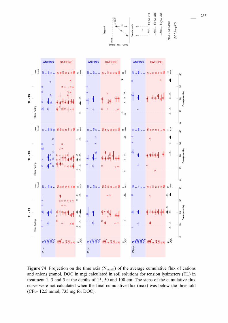
Part D : Soil solutions 255
Figure 74 Projection on the time axis (Nmonth) of the average cumulative flux of cations and anions (mmol, DOC in mg) calculated in soil solutions for tension lysimeters (TL) in treatment 1, 3 and 5 at the depths of 15, 50 and 100 cm. The steps of the cumulative flux curve were not calculated when the final cumulative flux (max) was below the threshold (CFt= 12.5 mmol, 735 mg for DOC).
05
1015
20
ANIONS CATIONS ANIONS CATIONS ANIONS CATIONS
HCl
NO
2
SO
4
NO
3
PO
4
Na
NH
4K M
gC
a
Al
Si
DO
C
15 c
m
HCl
NO
2
SO
4
NO
3
PO
4
Na
NH
4K M
gC
a
Al
Si
DO
C
50 c
m
HCl
NO
2
SO
4
NO
3
PO
4
Na
NH
4K M
gC
a
Al
Si
DO
C
100
cm
HCl
NO
2
SO
4
NO
3
PO
4
Na
NH
4K M
gC
a
Al
Si
DO
C
100
cm
010
2030
40max
(mm
ol)
Cle
ar F
ellin
g
3019
73-1
357
66
3267
275
37
4017
131
335
160
19
592
161
25
4 1 12961
11 2325
2558
328
1862
211
572
1 0 0120
2317
41
139
1357
7869
2029
1134
104
729
9767
125
907
556
10
101
2944
6
211
80
4947
1719
2368
13
1755
3472
6
8 1558
6929
532
109
480
130
71
535
4110
27
9 5448
1518
5704
63
1633
24
2913
1269
2940
94
1651
TL
- T
1
Dat
e (m
on
th)
010
2030
40max
(mm
ol)
Cle
ar F
ellin
g
6318
60
23-1
84
18016
1438
20
992
5712
7071
58
3 2 1320
2621
24
8319
434
14
3456
3252
428
1663
316
175
9629
2313
710
2 0119
3129
20
109
1363
146
375
131
5414
75
9447
33
5374
6
6319
524
11
4676
2177
949
60
3935
2315
2112
62
235
945
22
4574
1766
108
3054
102
278
5185
667
4921
4
11 -39225
49
2523
19
4291
116
2739
3001
193
61
TL
- T
3
Dat
e (m
on
th)
010
2030
40max
(mm
ol)
Cle
ar F
ellin
g
788
518
49
46-1
87
3265
13
323
3122
1315
300
372
34
105
6718
5 2 57539
2317
6 1572
1957
624
770
355
077
3 0 05431
45
5419
68
5179
2824
4011
8 5191
3530
14
200
071
0
3575
1912
689
1766
1676
3711
4220
131
10 1588
189
1551
8
203
075
130
76
12 655
78
-12
2319
1247
25
1487
3016
1414
2194
78
1612
42
TL
- T
5
Dat
e (m
on
th)
015
01
↑ ↓Δ_ _
_αC
Cum. Flux (mmol)
max
Dat
e (m
onth
)
Lege
nd
010
200510
~
h(%
) =
100 Δ
/max
h(%
)
h(%
)
h(%
)if
h(%
) <
10
if h(
%)
< 30
if h(
%)
> 30
(DO
C in
mg
L-1)
↑↑
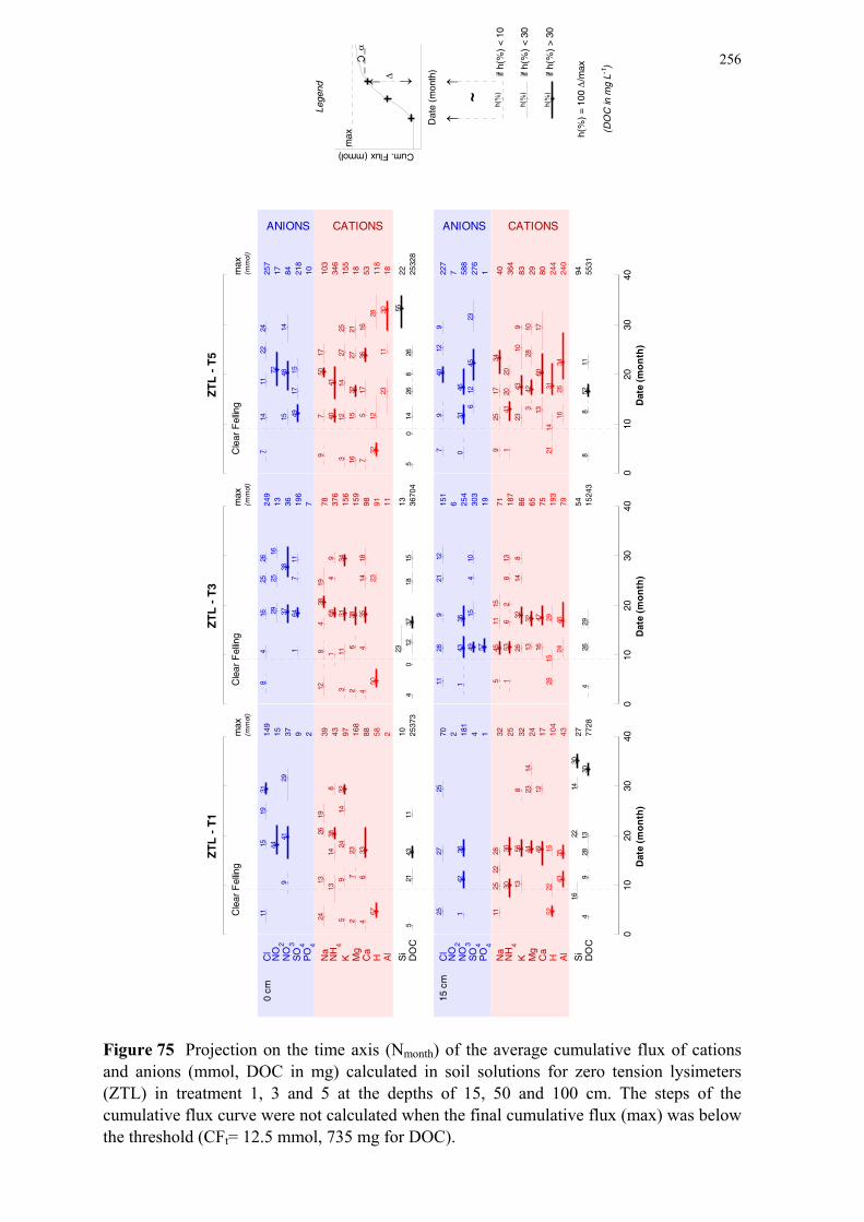
256
Figure 75 Projection on the time axis (Nmonth) of the average cumulative flux of cations and anions (mmol, DOC in mg) calculated in soil solutions for zero tension lysimeters (ZTL) in treatment 1, 3 and 5 at the depths of 15, 50 and 100 cm. The steps of the cumulative flux curve were not calculated when the final cumulative flux (max) was below the threshold (CFt= 12.5 mmol, 735 mg for DOC).
05
1015
20
ANIONS CATIONS ANIONS CATIONS
HCl
NO
2
SO
4
NO
3
PO
4
Na
NH
4K M
gC
a
Al
Si
DO
C
0 cm
HCl
NO
2
SO
4
NO
3
PO
4
Na
NH
4K M
gC
a
Al
Si
DO
C
15 c
m
010
2030
40max
(mm
ol)
Cle
ar F
ellin
g
5867
104
5222
15
149
1115
1931
7025
2725
1544
29 4379
4129
181
142
36
2 13924
1326
19
3211
2522
28
4313
1438
8
2530
30
975
924
1432
3213
568
168
27
23
2444
2314
884
633
1749
12
2 4343
35
10 2716
2214
30
2537
35
2143
11
7728
49
2813
30
ZT
L -
T1
Dat
e (m
on
th)
010
2030
40max
(mm
ol)
Cle
ar F
ellin
g
9150
23
193
2815
29
249
84
1625
26
151
1128
921
12
1329
2516
6196
164
711
303
4915
410
3637
38
254
143
36
7 1957
7812
84
3819
715
4511
15
376
168
49
187
153
62
813
156
311
3134
8626
3214
8
159
26
38
6513
32
984
435
1418
7516
47
11 7924
46
1323
543670
44
012
3718
15
1524
34
2629ZT
L -
T3
Dat
e (m
on
th)
010
2030
40max
(mm
ol)
Cle
ar F
ellin
g
118
3212
28
244
2114
31
257
714
1122
24
227
79
4012
9
1772
7218
4917
15
276
612
4523
8415
4814
588
031
46
10 1103
97
5017
409
2517
34
346
4041
364
141
2020
155
312
1427
25
8323
4310
9
1816
1532
2721
293
4228
10
537
517
3616
8013
6017
1823
1130
240
1626
34
2255
942532
85
014
268
26
5531
88
5211
ZT
L -
T5
Dat
e (m
on
th)
015
01
↑ ↓Δ_ _
_αC
Cum. Flux (mmol)
max
Dat
e (m
onth
)
Lege
nd
010
200510
~
h(%
) =
100 Δ
/max
h(%
)
h(%
)
h(%
)if
h(%
) <
10
if h(
%)
< 30
if h(
%)
> 30
(DO
C in
mg
L-1)
↑↑

Part D : Soil solutions 257
The curves of cumulative fluxes are composed of five main steps ( Figure 74 & Figure 75),
which occurrences depend on the element analyzed, the collector type, the collection
depth, and the treatment:
• The 1st step occurs before CF just after the 1st drought at Nmonth=4 and can be
observed in all treatments, but only in ZTL since no data were available for TL
before CF.
• The second step occurs for solutions collected by TL and ZTL at planting at
Nmonth=11 (fertilization 1, CF+2) and corresponds to the end of the rainy season.
Leaching of all elements occurs down to a depth of 50 cm.
• The third step occurs from Nmonth=17 to Nmonth=20 and corresponds to a period of
intensive drainage after the winter drought, followed by the second fertilization.
Leaching of all elements occurs down to a depth of 1 m within 1 to 2 months.
• The last two steps occur at Nmonths=25 and 30-31. They correspond to the end of
the 2005 summer and to the end of the winter (intensive drainage after drought)
respectively, and to the 3rd and 4th fertilization respectively. Leaching occurs for
only small contents of mobile anions and cations down to a depth of 15 cm.
The first step of nutrient fluxes corresponds to the mineralization of the forest floor in
the old E. saligna stand before it was clear felled and is interesting to observe since it is not
polluted by nutrients released by the fertilizers. Although it can only be studied in ZTL, it
suggests a strong recycling of Ca, Mg and K in the upper soil layers by the Eucalyptus
trees. NO3 appears in soil solutions at a depth of 15 cm. Since no NH4 is observed in the
solutions, we can assume that NH4 is preferentially taken up by plants, immobilized by
micro-organisms or very quickly nitrified. Eucalyptus trees are known to take up NH4 or
NO3 or both chemical forms depending on the species and the geographical site
(Smethurst, 2000) so that this result is not surprising. A preferential uptake of NH4 over
NO3 has already been observed for Eucalyptus in Brazil (Vale et al., 1984).
The nutrients released by the mineralization of the organic matter (harvest residues,
forest floor and soil organic matter) and of the sewage sludge, and by the dissolution of the
first fertilization are firstly leached just after planting down to a depth of 15-50 cm (2nd
step), but the main leaching occurs with the first heavy rainfall after the winter drought and
reaches a depth of 1 m within two months (3rd step). This suggests that, after planting,
either the drainage is not large enough to transport the solutes in deeper soil layers, or the
dissolved nutrients are adsorbed and/or immobilized and/or taken up in the upper soil

Part D : Soil solutions 258
layers. The limited rainfall of the winter period together with the transpiration of the
Eucalyptus trees allow a slow transfer of the concentration front to deeper soil layers which
may explain that it takes six months for the concentrations to reach a depth of 100 cm
whereas the nutrient fluxes are not delayed. The first heavy rainfall washes the soil profile
and pushes the elements down to deeper soil layers where free exchanger surfaces are
available. This nutrient leaching is increased by the dissolution and mineralization of the
2nd fertilization and the activation of the mineralization of the forest floor. Ionic strengths
are greater and so is the competition of anions and cations for exchange sites, which
participates in leaching nutrients deeper in the soil profile.
The last two periods of leaching (3rd and 4th steps) correspond to the mineralization of
the forest floor and/or to the dissolution of the next two fertilizations (KCl in all treatments
and ammonium sulphate in T3) and remain localized in the upper 15 cm of the soil profile.
The chemical associations observed for concentrations were confirmed by the
observation of the nutrient fluxes.

Part D : Soil solutions 259
D.2.5.4.2 Total cumulative fluxes from the clear felling until two years after planting
0 1 2 3
PiThStZTL 0 cm
15 cmTL 15 cm
50 cm100 cm300 cm
0 1 2 3
PiThStZTL 0 cm
15 cmTL 15 cm
50 cm100 cm300 cm
0 1 2 3
PiThStZTL 0 cm
15 cmTL 15 cm
50 cm100 cm300 cm
0 1 2 3
PiThStZTL 0 cm
15 cmTL 15 cm
50 cm100 cm300 cm
0 1 2 3
PiThStZTL 0 cm
15 cmTL 15 cm
50 cm100 cm300 cm
0 500 1000
(T1,T3)<T5
T1<T5
Cl: Total flux (mmol)0 500 1000
(T1,T3)<T5
T1<T5
NO3: Total flux (mmol)
0 200 400 600
T1<T5
(T1,T3)<T5
NO2: Total flux (mmol)
0 200 400 600
(T1,T5)<T3(T1,T5)<T3
SO4: Total flux (mmol)
0 200 400 600H
2PO
4: Total flux (mmol)
0 200 400 600DOC: Total flux (g)
0 200 400 600
T3<(T1,T5)
T5<T1T5<T3
Na: Total flux (mmol)0 200 400 600
(T1,T3)<T5
T1<T3
K: Total flux (mmol)0 200 400 600
T1<T5
T1<T5
NH4: Total flux (mmol)
0 200 400 600
T5<(T1,T3)
(T1,T5)<T3T5<T3
(T1,T5)<T3
Mg: Total flux (mmol)0 200 400 600
(T1,T3)<T5
(T1,T5)<T3
Ca: Total flux (mmol)0 200 400 600
Fe: Total flux (mmol)
0 200 400 600Al: Total flux (mmol)
0 200 400 600
(T1,T3)<T5
T1<T5T1<T3<T5
T1<T5
T3<T5
H: Total flux (mmol)0 200 400 600
Si: Total flux (mmol)
0 2 4 6 8 10 12 14 16 18 20
Average Treatment 1
Average Treatment 3Average Treatment 5
Standard error Treatment 1
Standard error Treatment 3Standard error Treatment 5
Figure 76 Mean cumulative fluxes and standard errors (when n=3) calculated from the clear felling (Nmonth=9) to the end of the experimental period (Nmonth=37) for cations and anions measured in soil solutions for each collector type (Pi=Rainfall, Th=Throughfall, St=Stemflow, ZTL=zero tension lysimeter, TL=tension lysimeter), collection depth and treatment. Differences among treatments are indicated when significant at P<0.05.
Part D : Soil solutions 260
The greatest total cumulative fluxes (from the clear felling until the end of the
experimental period) were found for NO3 (about 500 mmol from a depth of 15 cm down to
a depth of 100 cm in all treatments), then for Cl (about 300 mmol from the forest floor
down to a depth of 100 cm), SO4 and NH4 in T3 and T5 (about 300 mmol from the forest
floor down to a depth of 15 cm, except in TL for NH4). Total cumulative fluxes for H, Al,
K, Mg and Ca came next with greatest total fluxes from 100 and 200 mmol ( Figure 76).
Standard errors were large in particular for Cl, SO4, H2PO4, NH4, Ca and K, so that
few significant differences could be observed. Qualitatively, the order of decreasing total
flux for NO3, H and Al was T5 > T3 > T1 whatever the depth. SO4 fluxes were large only
in T3 and T5 and found deeper in T3 (down to a depth of 50 cm) than in T5 (down to a
depth of 15 cm). Mg total fluxes were less in T5 (where dolomitic lime was not applied)
than in T1 and T3 and reached deeper soil layers in T3 (down to a depth of 50 cm) than in
T1 and T5. In general, the largest values were reached in the forest floor or at a depth of 15
cm then total fluxes decreased with depth. More NH4 was leached in the forest floor and at
a depth of 15 cm in T3 and T5 than in T1. The main significant differences showed:
• larger cumulative fluxes of nitrates, H and NH4 in T5 than in other treatments at
the depths of 15 and 50 cm for nitrates, and in the forest floor and at a depth of 15
cm for H and NH4
• smaller cumulative fluxes of Na and Mg in T5 than in other treatments at depths of
50 cm (T1) and 100 cm (T3) for Na, and in the forest floor for Mg,
• larger cumulative fluxes of sulphates, Ca and Mg in T3 than in other treatments at
the depths of 15 (sulphate and Mg only) and 50 cm,
Differences among treatments could not be studied for Al, Fe, Si and DOC since one
single composite sample per treatment was analyzed.
This quantitative analysis confirms that ammonium and nitrates are released together
with H and Al in the upper soil 15 cm of the soil profile (no increase of total flux below
this depth). The ammonium cumulative flux is large only in the forest floor and in the
upper soil layers (15 cm) which suggests that an excess of NH4 is quickly released in soil
solution before nitrification occurs or that NH4 is only partly nitrified. It also confirms that
ammonium, nitrate and aluminium releases are in the following order: T5 > T3 > T1. The
same quantitave trends among treatments are observed for H but only in the upper soil
layer (15 cm) which would confirm an increase in the system buffering capacity when

Part D : Soil solutions 261
fertilizers are applied as already suggested in § D.2.5.3. On the contrary, aluminium began
to decrease only below a depth of 50 cm together with nitrate.
The depths of presumed adsorptions for anions are also confirmed: NO3 mainly from
100 cm down to 300 cm, SO4 from a depth of 15 cm down to a depth of 50-100 cm in T3
and of 50 cm in T5, and H2PO4 from the soil surface down to a depth of 50 cm in T3 and
of 15 cm in T5. Immobilization in the organic matter and/or microbial biomass and uptake
by the fast growing Eucalyptus trees may also have occurred at the same depths, especially
for NO3. In T5, smaller cumulative fluxes of Mg confirm the results of the vegetation
dynamics which showed smaller Mg contents in the Eucalyptus of T5 than of T1 and T3.
D.2.5.4.3 Dynamics at the end of the experimental period
Table 41 Slope (mmol L-1 or g L-1 for DOC) of the tangent to the cumulative flux curve at the end of the experimental period for each collector type (ZTL=zero tension lysimeter, TL=tension lysimeter), collection depth and treatment (T). The slopes are given in bold when there value was above the threshold for nutrient flux SC’t=1 mmol month-1 (0.06 g month-1 for DOC).
H Cl NO2 NO3 SO4 PO4 Na NH4 K Mg Ca Fe Al Si DOC T mmol g
ZTL 0 cm 1 2.0 <0.5 5.8 3.2 0.1 3 <0.5 <0.5 <0.5 0.9 5.2 1.0 <0.5 <0.5 <0.03 5 5.3 2.4 0.9 1.0 <0.5 1.1 4.0 0.2
15 cm 1 <0.5 <0.5
<0.5
1.6<0.5
<0.5 3.2 1.2 3 1.6 <0.5 3.4 0.6 <0.5 1.7 1.0 1.1 1.7 0.3 5 3.8 0.6 11.0 2.5 0.6 4.4 2.7 <0.03
TL 15 cm 1 1.2 <0.5 3.6<0.5 <0.5
5.9 0.5 3 <0.5 <0.5 3.8 <0.5 1.1 1.7 <0.5 0.7 5 2.8 1.1 4.8 1.9
<0.5
<0.5 0.6 <0.03
50 cm 1 <0.5 <0.5 2.4 1.1 0.9 3 4.9 2.1
<0.5
<0.5 0.8 5
<0.5 2.3
<0.5
<0.5 0.8 47.0 <0.03
100 cm 1 11.0 0.5 2.4 0.9 1.5 3.6 0.7 3
<0.5
4.1 1.3 1.1 <0.5 0.8 5 1.9 6.1 2.7 1.8 0.4
300 cm 1 0.9 3 <0.03 5
<0.5 <0.5
<0.5
<0.5
<0.5
<0.5 <0.5
<0.5 <0.5
<0.5<0.5
<0.5
<0.5 <0.5
0.1

Part D : Soil solutions 262
The increasing trends for H, Cl, Al, NO3 and SO4 observed at the end of the experimental
period in T5 in the forest floor and at a depth of 15 cm ( Table 41) suggest that the sewage
sludge is not completely mineralized in T5, as confirmed on field by visual observations of
remaining sludge.
The increasing trends observed at the depth of 1 m for H, NH4, Al, Cl and SO4 suggest
that the dynamics of downward transfer of the mineral elements issued from the clear
felling and the fertilizer applications are still running at a depth of 1 m. At a depth of 300
cm, no increasing trend above the thresholds is recorded, which means that this downward
transfer did not reach a depth of 3 m yet. The increasing trends of Mg and Ca beneath the
forest floor, and of NO3, NH4, H and Al in the upper soil layers may be explained by the
mineralization of the forest floor which occurs continuously all over the stand rotation, first
from the harvest residues left on floor after clear felling, then from the litterfall of the new
stand which started after about one year of growth.

Part D : Soil solutions 263
D.3 CONCLUSIONS
D.3.1 On the dynamics of nutrients in soils
Concentration and fluxes of nutrients in the soil solution were thus driven by two main
processes:
• The mineralization of the harvest residues, of the forest floor and of the soil
organic matter followed by the nitrification of the ammonium, released H, Al and
NO3 in the upper layers of the soil profile (0-15 cm). This release was enhanced by
the nitrification of the fertilizers in particular in T5 (sewage sludge). Dissolution of
other fertilizers together with specific adsorption of S and P probably buffered the
protons release in all treatments and more particularly in T3,
• The dissolution of the fertilizers released nutrients in soil solutions in their original
chemical association (K/Cl and NH4/SO4 in T3), but SO4 was quickly
reorganized with Mg and Ca, enhancing Mg and Ca mobility. Mg and Ca came
from the mineralization of the forest floor, the dissolution of the dolomitic
limestone in T1 and T3, and the mineralization of the sewage sludge in T5 (mainly
Ca since the sewage sludge was Mg-poor). These dissolutions were highly
heterogeneous in time and space (localized under the fertilizer pocket buried at the
tree stem in T1 and T3, and below the sewage sludge line in T5). Mineralization of
the sewage sludge and dissolution of the mineral fertilizers were still running at the
end of the experimental period but with a weak intensity.
Nutrients released in soil solution were quickly transported to deeper soil layers first
after clear felling and planting, and mainly with the first heavy rainfall following the dry
period after planting. Between the periods of large drainage, slower diffusion processes
and chemical reorganizations occurred within the soil profile. The nutrient front reached
the depth of 1 m but was never observed at a depth of 3 m so that even if very large
concentrations of all elements were observed in upper soil layers the concentrations at the
outlet of the studied soil profile always remained below the thresholds of groundwater
quality. The doubt remained whether the nutrient flux was stopped because nutrients were
adsorbed, immobilized or taken up between the depths of 1 to 3 m or simply because there

Part D : Soil solutions 264
was no water enough to transport them due to the high transpiration of the Eucalyptus
trees.
The soil solution study suggested that, once released in soil solutions, NO3 was
adsorbed on soil surface (or immobilized or taken up) between the depths of 1 to 3 m
together with Al, SO4 was adsorbed from a depth of 15 to 100 cm in T3 and to 50 cm in
T5, and H2PO4 from a depth of 15 to 50 cm in T3. These hypotheses are in good agreement
with the potential adsorptions capacity measured in part B but are to be checked.
As ammonium was never observed in soil solutions except when quickly dissolved
from the fertilizer together with sulphate, it is suggested that Eucalyptus trees preferred
ammonium to nitrate, but ammonium may also have been quickly nitrified.
D.3.2 On the methods used
In part C, it was shown that the water drainage model systematically overestimated the
water fluxes in the plantation especially at a depth of 50 cm, but that the flux at the outlet
of the soil profile was accurate since it was fixed as the lower boundary of the soil profile.
The same trends are thus to be expected for nutrient fluxes. Moreover, the spatial
heterogeneity at the tree scale was not accounted for in the water drainage model but
spatial patterns of nutrient concentrations were observed in soil solutions in particular near
the tree stem where the water drainage is thought to be heterogeneous (stemflow input and
higher fine root density than in the inter-row). Spatial heterogeneity of the water flux
should be integrated in the model to compute more accurately nutrient fluxes. The spatial
heterogeneity of the nutrient input by stemflow and by localized application of fertilizers is
also essential in case of geochemical modelling, together with the knowledge of the rates
of dissolution and/or mineralization of the fertilizers.
The type of data analysis enabled to study the nutrient dynamics in its continuity with
simple analytical tools. Compared to discontinuous analysis, this method allows an easier
comparison of the concentration events from one treatment or collector to another (onset,
intensity, delay of maximum intensity, end). This first approach may be completed by the
use of more powerful softwares of spectra analysis which would enable more sensitive
calculations of the peaks characteristics and quantitative calculations of the peak areas.
Statistical analysis may then be performed on these characteristics to study more precisely
the effect of spatial heterogeneities or treatments on the soil solution chemistry and the

Part D : Soil solutions 265
correlations among mineral elements. This method would be quite useful since statistical
analysis usually performed on soil solution concentrations do not respect independency
hypotheses.
The thresholds used in the present study were defined as to observe the appearance and
attenuation of the main concentration peaks issued from the clear felling and from the
fertilizer applications. As the influence of these ecosystem perturbations will decrease with
time, lower thresholds will have to be defined, for example using the major concentration
peaks observed in aboveground solution collectors.


267
PART E
NUTRIENT BUDGETS


Part E: Nutrient budgets 269
INTRODUCTION
Over the studied period, the soil solution chemistry experienced changes under the
influence of the silviculture (clear felling and fertilizing) and of the stand development.
Large contents of mineral elements were leached down to the depth of 1 m, but the
question remains about what happened of these elements between the depths of 1 to 3 m,
and which part of the fertilizers (in particular K, Ca, Mg and P) has been dissolved or
mineralized and subsequently taken up by the fast growing Eucalyptus trees since they did
not appear in large quantities in soil solution. The system D of Figure 2 shows that the
interactions of the soil solution with i) the vegetation, (ii) the soil surface and the soil
matrix, and (iii) the soil organic matter and microbial biomass, account for the differences
between the amounts of mineral elements released in the soil solution (from the
mineralization of the forest floor and of the sewage sludge in T5 and from the dissolution
of the fertilizers in T1 and T3) and the mineral elements leaving the soil solution system by
leaching at a depth of 3 m.
The vegetation monitoring showed, as reminded in part A, a strong recycling of
mineral elements in the forest floor and in the upper soil layers as already observed in
others Eucalyptus plantations (Laclau et al., 2003c). This pattern suggests that a great part
of the fertilizers were directly taken up by the trees without being observed in the soil
solutions experimentally collected.
The soil study of part B showed that the soil mineral constituents could mainly
released Fe, Al, Si and H in the soil solution. The potential for adsorption of cations on the
soil surface was < 1 cmolc kg-1 but was highly pH dependant. The CEC was mainly
saturated with Al so that basic cations may be adsorbed on the CEC provided the fact that
either the CEC increases or Al is released in soil solution. The anion exchange capacity
may lead to an adsorbption of anions especially below a depth of 1 m. Specific adsorptions
may result in large retention of S and P in soils from the upper soil boundary down to a
depth of 3 m. This seems in good agreement with the observations of the soil solution
chemistry but mineral elements actually adsorbed on the soil surface remain to be checked.
Water drainage is essential in the computation of mineral element fluxes. Part C
showed that (i) even if the water flux is probably overestimated at the depths of 15, 50 and
100 cm, the water flux at a depth of 3 m is likely to be accurate since it was fixed as the

Part E: Nutrient budgets 270
lower boundary of the studied profile (provided the fact that the hypothesis of a single
porosity is accurate), and (ii) a large water uptake of the fast growing Eucalyptus stand
which limited the water drainage at a depth of 3 m to less than 5% of the incoming rainfall
(in average) from six months after planting onwards. Drainage occurs at this depth during
the wet season at a small constant rate (1 mm day-1) or after large rainfall events
(Nmonth=21 & 36) and upward flow (about 1 mm day-1) occurs during the dry periods. In
part D, it was shown that nutrients realeased in soil solutions after clear felling and
fertilizing were mainly transported in deep soil layers with the first heavy rainfall
following the dry period after planting at Nmonth=17-18. The nutrient flux reached a depth
of 1 m within 2 months so that we can assume that it would have reached a depth of 3 m
within, at least, 2 to 4 more months, that is, at Nmonth=22-24. Since water drainage at a
depth of 3 m decreased sharply after Nmonth=21 ( Figure 50), a doubt remains whether the
mineral elements transported in the soil solution at a depth of 1 m did not leave the soil
profile because they had been taken up, adsorbed or immobilized in the soil organic matter
and microbial biomass, or simply because there was no water enough to transport them.
Quantitative study of the global budget of the system may help rule on the hypotheses
formulated. As already mentioned in the general introduction of this thesis, system D (soil
solution) will not serve to compute nutrient mass budgets because two many fluxes are
impossible to measure and to compute. System A (tree+soil+soil solution) will thus be
preferred to compute mass budgets as all major fluxes of this system were experimentally
measured. The main goal of this part is to check by simple mass budget wether the
hypotheses formulated in parts A, B, C and D are consistant with the mass transfers among
storage compartments occurring during the experimental period. The computed budgets are
not fertility budgets of the plantation.
The nutrient budgets are established for K, Ca, Mg, P and N in priority since these
elements were quantified in the trees. The organic part of the soil system was not studied in
this thesis but its influence on the mass budget is discussed.

Part E: Nutrient budgets 271
E.1 MATERIAL AND METHODS
E.1.1.1 Studied system and times of observations
The studied system was the system A of Figure 2 already presented in the general
introduction of this thesis, that is, the whole stand plus the soil and the soil solution down
to a depth of 3 m. The system was observed from the clear felling until 24 months after
planting.
We already mentioned that the Eucalyptus root system reaches soil depths > 3 m
within 1 year of growth. As the studied systems stops at a depth of 3 m, a supplementary
flux should be added on Figure 2-A: the root uptake and exudates occurring below a depth
of 3 m. Here, we suppose that all nutrients are taken up in the 0-3 m soil layer and that
these fluxes, although substantial for water uptake, are insignificant for nutrient uptake.
The very low contents of available nutrients measured in soils below a depth of 3 m in part
A would confirm this hypothesis but it remains to be checked.
It has to be reminded that the water uptake (evapotranspiration) estimated in part C
was optimized by comparing the simulated water contents to the measured soil moistures
down to a depth of 3 m, with the lower boundary of the soil profile fixed as the measured
soil moisture at a depth of 3 m. The evapotranspiration thus estimated corresponded to the
effective uptake within the upper 3 m of the soil profile and did not account for the
Eucalyptus uptake from deeper soil layers, so that the water budget performed in part C
was accurate.
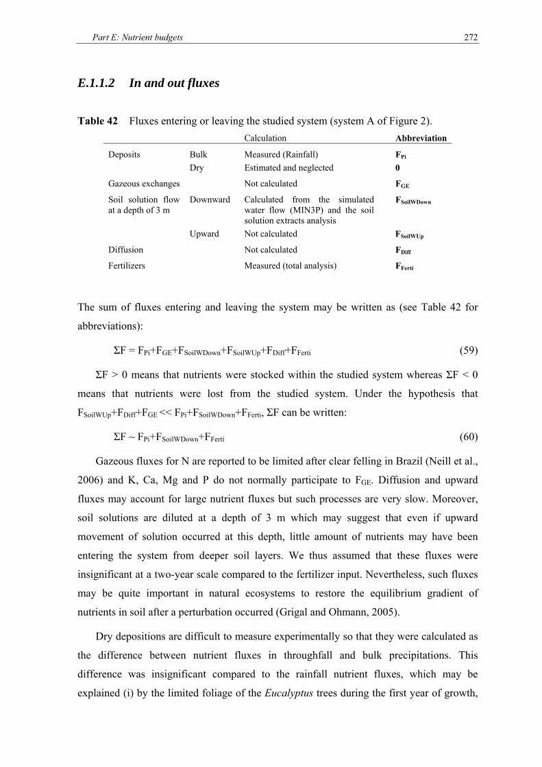
Part E: Nutrient budgets 272
E.1.1.2 In and out fluxes
Table 42 Fluxes entering or leaving the studied system (system A of Figure 2). Calculation Abbreviation
Deposits Bulk Measured (Rainfall) FPi Dry Estimated and neglected 0
Gazeous exchanges Not calculated FGE
Soil solution flow at a depth of 3 m
Downward Calculated from the simulated water flow (MIN3P) and the soil solution extracts analysis
FSoilWDown
Upward Not calculated FSoilWUp
Diffusion Not calculated FDiff
Fertilizers Measured (total analysis) FFerti
The sum of fluxes entering and leaving the system may be written as (see Table 42 for
abbreviations):
ΣF = FPi+FGE+FSoilWDown+FSoilWUp+FDiff+FFerti (59)
ΣF > 0 means that nutrients were stocked within the studied system whereas ΣF < 0
means that nutrients were lost from the studied system. Under the hypothesis that
FSoilWUp+FDiff+FGE << FPi+FSoilWDown+FFerti, ΣF can be written:
ΣF ~ FPi+FSoilWDown+FFerti (60)
Gazeous fluxes for N are reported to be limited after clear felling in Brazil (Neill et al.,
2006) and K, Ca, Mg and P do not normally participate to FGE. Diffusion and upward
fluxes may account for large nutrient fluxes but such processes are very slow. Moreover,
soil solutions are diluted at a depth of 3 m which may suggest that even if upward
movement of solution occurred at this depth, little amount of nutrients may have been
entering the system from deeper soil layers. We thus assumed that these fluxes were
insignificant at a two-year scale compared to the fertilizer input. Nevertheless, such fluxes
may be quite important in natural ecosystems to restore the equilibrium gradient of
nutrients in soil after a perturbation occurred (Grigal and Ohmann, 2005).
Dry depositions are difficult to measure experimentally so that they were calculated as
the difference between nutrient fluxes in throughfall and bulk precipitations. This
difference was insignificant compared to the rainfall nutrient fluxes, which may be
explained (i) by the limited foliage of the Eucalyptus trees during the first year of growth,

Part E: Nutrient budgets 273
and/or (ii) by the fact that bulk deposition collectors already collected a great part of the
dry depositions. It was further neglected in ΣF.
The fluxes were calculated from the results of part D which means that losses of
organic N were not accounted for in the nitrogen budget since DON was not measured in
soil solutions.
E.1.1.3 Changes in nutrient stocks
E.1.1.3.1 Stocks of the studied system
The main compartments of the studied system are detailed in Table 43.
Differences in stocks from clear felling to two years after planting can be written as
(see Table 43 for abbreviations):
ΔS = ΔSSt1 + ΔSAB2 + ΔSFF1 + ΔSRem + ΔSFF2 + ΔSR1 + ΔSR2 + ΔSFerti + ΔSSoilS +
ΔSSoilM + ΔSSoilW + ΔSSoilMB (61)
ΔS > 0 means that nutrients were stocked within the system whereas ΔS < 0 means
that nutrients were lost from the system. Only the terms in bold were measured and
calculated in the present budget:
ΔSmeasured = ΔSAB1 + ΔSAB2 + ΔSFF1 + ΔSRem + ΔSFF2 + ΔSR1 + ΔSR2 + ΔSSoilS (62)
The mass conservation implies that:
ΔS = ΣF (63)
or equally:
ΣF – ΔSmeasured = ΔSFerti + ΔSSoilM + ΔSSoilW + ΔSSoilMB (64)
Equation (64) shows that the differences between the measured fluxes and the
measured changes in stocks may be explained by changes in stocks of fertilizers (ΔSFerti),
soil solution (ΔSSoilW), soil mineral matrix and soil organic matter (ΔSSoilM), or soil
microbial biomass (ΔSSoilMB).
The stocks in the soil mineral matrix may be considered invariants for Ca, Mg and K
(ΔSSoilM=0) since no mineral which may release such elements were found in the
mineralogical study of part B, but differences in soil mineral stocks of S, P and Al may
have occurred.

Part E: Nutrient budgets 274
Soil organic stocks (soil and microbial biomass) were neither measured nor calculated
but they may account for a great part of the observed differences in ΣF in particular for N.
In this thesis, we focused on mineral elements but specific studies of the organic part of the
system are currently being carried out in the experiment.
The fraction of the fertilizers (ΔSFerti) which remained at the end of the experiment
may be large for low solubility fertilizers such as dolomitic limestone, as well as for the
sewage sludge which may last to mineralize. On the contrary, KCl and (NH4)2SO4 may
dissolve quickly and ΔSFerti may be insignificant for these minerals.

Part E: Nutrient budgets 275
Table 43 Stocks of the studied system at clear felling (T0) and two years after planting (Tf). T0 (Nmonth=9) Tf (Nmonth=37) Calculation Abbreviation
Aboveground biomass
From the previous rotation Stump Remaining unmineralized Considered invariant ΔSSt1
From the new planted stand 0 Bark, leaves, branches stem, stump
Direct measurement at Tf ΔSAB2
Forest floor and remnants
From the previous rotation Left on floor Remaining unmineralized Direct measurement on site at T0, and from an adjacent plot kept free from remnants and vegetation at Tf
ΔSFF1
Bark, leaves, branches Left on site as remnants
Remaining unmineralized Direct measurement at T0 and estimated from decomposition rates measured in litter bags
ΔSRem
From the new planted stand 0 Fallen minus mineralized during the period
Direct measurement at Tf ΔSFF2
Belowground (roots)
From the previous rotation Remaining at the end of the rotation
Remaining unmineralized Direct measurement at T0 and estimated from decomposition rates measured in litter bags
ΔSR1
From the new planted stand 0 2 years-old Direct measurement at Tf ΔSR2
Fertilizers Forest floor + soil (T1, T3)
0 Remaining undissolved or unmineralized
Not calculated ΔSFerti
Soil Surface of soil constituents Estimated from soil specific extractions ΔSSoilS
Matrix (minerals + soil organic matter)
Not calculated ΔSSoilM
Solution Not calculated ΔSSoilW
Microbial biomass Not calculated ΔSSoilMB

Part E: Nutrient budgets 276
E.1.1.3.2 Measurements and calculations
The main terms of eq (61) represent (i) the changes in stocks of nutrients in the Eucalyptus
trees and (ii) the changes in stocks of nutrients adsorbed (more or less specifically) on the
soil constituents surface. The vegetation stocks were taken from Laclau et al (2004b;
2005b; 2007) as presented in part A. Specific extractions were performed on soils to
quantify the elements effectively adsorbed and are described thereafter.
For the quantification of adsorbed elements, a new soil sampling was performed 2
years after planting (AP24). In May 2006, soil samples were collected for one pit per block
and treatment, in treatments 1, 3 and 5, blocks 1, 2 and 3, and from three pits excavated in
part of the former stand kept uncut (named reference – R). In each pit, soils were sampled
at the depths of 0-5 cm, 5-15 cm, 15-30 cm, 30-50 cm, and 50-100 cm. In block 1 and all
blocks of treatment 3 and reference, supplementary samples were collected at the depths of
50-100 cm, 100-200 cm, and 200-300 cm. Samples were taken continuously from the tree
stem to the inter-row to integrate the soil spatial heterogeneity at the tree scale.
The soils of the reference plot were considered to be equivalent to the soils of the
experiment at clear felling. In fact, the soils thus sampled had experienced more two years
of growth of the E. saligna stand, but as this stand was more than 6 years-old, it may be
considered at a steady-state compared to the major perturbations occurring at clear felling,
fertilizing, and re-planting. The soil status after two years of growth was compared to this
reference preferentially than to the soils sampled before clear-felling (data set SOILBCF of
part B) because (i) extractions on fresh soils for nitrates and ammonium were needed but
had not been performed on the SOILBCF sampling, and (ii) the concentrations measured in
the soil extracts are generally very small for such soil type (CEC & AEC < 1 cmolc kg-1,
saturations in basic cations < 0.1 cmolc kg-1) and analytical series are very sensitive to the
experimental conditions at the time of the extraction (deionized water, ambient conditions,
equipment calibration, …). We preferred comparing samples from the same experimental
series than risking an analytical bias when using data of the SOILBCF analytical series.
Once collected, fresh soils were immediately extracted with (i) distilled water, and (ii)
KCl 2 mol L-1 using a soil-solution ratio of 1/10 (Mulvaney, 1996). After a 1-hour shaking,
the soil suspensions were filtered and kept at 4°C. In the water extracts, Ca, Mg, Na, NH4,
NO3, SO4 and H2PO4 concentrations were measured by ion chromatography (CENA,
Laboratorio de Ecologia Isotopica) and Al by ICP (CENA, Laboratorio de Química

Part E: Nutrient budgets 277
Analítica). K and Cl were also measured in the water extracts but the results were
discarded since contamination of KCl occurred during the extractions performed in the
field. In the KCl extracts, NH4 and NO3 concentrations were measured by colourimetry
(CENA, Laboratorio de Biogeoquímica Ambiental).
The soils were subsequently air-dried. The CEC was measured following the same
protocol than in the soil section (§ B.1.1.2). Sulphates were extracted by H2PO4 (ratio 2/5)
and measured by turbidimetry (Cantarella and Prochnow, 2001). Phosphates were
extracted by the Mehlich 1 protocol (ratio 1/10) and measured by colourimetry (da Silva et
al., 1999). The extractions were performed at ESALQ, Departamento de Ciências do Solo,
Laboratorio de Analises Químicas-Pesquisa.
Classically, successive extractions are recommended to extract the whole pool of
adsorbed sulphate (Delfosse, 2005; Prietzel et al., 2001) but the available
photocolourimeter was not sensitive enough to small concentrations. KH2PO4 is also
reported to extract about 50 % of the S pool in acidic forest soils that received much S
from the atmosphere or from gypsum or ammonium sulphate fertilizations (Prietzel and
Hirsch, 2000). In the same way, the Mehlich method is reported to extract available P
(Kuo, 1996), which means that a great part of the adsorbed P may not have been extracted
by this method. These extractions give a good idea of the relative distribution of the S and
P adsorbed at clear felling and two years after planting according to the soil layer sampled.
Nevertheless, their absolute values must be handled cautiously since they are likely to
underestimate the whole pool of adsorbed S and P.
Computing differences in stocks in the soil is highly problematic: little changes in the
studied variable may be confounded with spatial heterogeneity or analytical variations and
when integrated over the entire soil mass these tiny values may represent very large
amounts. To preclude summing non significant differences over the whole soil profile, two
thresholds were defined
• a threshold of analytical determination estimated by diluting standards until the
measured data differed > 10 % from the theoretical one,
• a threshold of analytical repeatability: 3 replicate analysis were performed for one
sample per depth, and differences between two samples for a given depth were
considered significant when larger than twice the standard error of the 3 replicate
analyses.

Part E: Nutrient budgets 278
Differences in stocks of adsorbed nutrients were computed for all cations (except NH4)
from the CEC measurements, for NO3 and NH4 from the KCl extractions performed on
soils at field moisture, and for S and P from extractions by KH2PO4 and by the Mehlich
protocol, respectively.

Part E: Nutrient budgets 279
E.2 RESULTS AND DISCUSSION
E.2.1 Nutrient fluxes entering and leaving the studied system
0
100
200
300
400
Cl N S P Na K Mg Ca Al
Flux
(kg/
ha)
Influx
ZTL15
TL15
TL50
TL100
TL300
T5
0
100
200
300
400
Cl N S P Na K Mg Ca Al
Flux
(kg/
ha)
Influx
ZTL15
TL15
TL50
TL100
TL300
T3
0
100
200
300
400
Cl N S P Na K Mg Ca Al
Flux
(kg/
ha)
Influx
ZTL15
TL15
TL50
TL100
TL300
T1
Figure 77 Total nutrient influx (fertilizer + total atmospheric deposits) and amounts of nutrients leached in soil solutions (estimated from part D) at the depths of 15, 50, 150 and 300 cm from the clear felling until age two years in the fertilization experiment for treatments 1 (T1), 3 (T3) and 5 (T5). Vertical bars stand for standard errors (in T3 at 50 cm and in T5 at 100 cm and 300 cm, n=6; in T3 at 100 cm and 300 cm n=12; n=3 elsewhere). TL=Tension lysimeter, ZTL= Zero tension lysimeter.
Part E: Nutrient budgets 280
As already mentioned in part D, almost no nutrient was leached at a depth of 3 m. To help
understanding the nutrient dynamics within the studied system, nutrients fluxes at depths <
300 cm will be compared to nutrient inputs, but total budgets should not be performed at
these depths since other fluxes such as tree uptake in deeper soil layers should be
accounted for.
About 50 to 100 % of the chloride entering the system was leached down to a depth of
100 cm ( Figure 77). This flux was poorly attenuated between the depths of 15 to 100 cm.
In T1, a release of chloride in soil solution seemed to occur between the depths of 50 to
100 cm but the spatial heterogeneity associated to this flux was high.
The sulphate fluxes confirmed the observations made in part D. In T1 almost no S
entered or left the studied system. Almost all the S applied was leached at a depth of 15 cm
in T3 and in ZTL of T5. S fluxes were rapidly attenuated in deeper soil layers. The
amounts of S leached were of the same order of magnitude as measured in European soils
which received 75 kg N ha-1 year-1 through (NH4)2SO4 fertilizers (Carnol et al., 1997).
Almost none of the P applied was leached at a depth of 15 cm in T1 and T5. In T3, the
P fluxes at a depth of 15 cm equaled the P influx. The spatial heterogeneity associated to
this flux was very high so that it may correspond to localized dissolutions of P.
When no N was applied (T1), N leaching was greater than the N influx down to a
depth of 50 cm which confirmed that nitrate and ammonium were released in the soil
solution in the upper layers of the soil profile (about 65 kg ha-1). Larger amounts of N were
leached in T3 and T5 than in T1 as already mentioned in part D, but these amounts were
far less than the N brought by the fertilizers. If we attribute 65 kg N ha-1 of these amounts
to the mineralization of the harvest residues and of the organic matter as in T1 (part A),
then about 10 % of the N from the fertilizers were leached in T3 (25 kg N ha-1) and in T5
(35 kg N ha-1) at the depth of 50 cm. Comparatively in the forests of England, 77 and 113
kg ha-1 of N-NO3 where leached after clear felling and clear felling + fertilizing with 75 kg
N ha-1 of (NH4)2SO4, respectively (Carnol et al., 1997). In the US forests, 60-90 kg N-NO3
ha-1 year-1 were leached down to a depth of 1 m after bole-only harvesting (Strahm et al.,
2005). This pattern would confirm, as reviewed by Zech et al. (1997), that the dynamics of
soil organic matter share common features in temperate and tropical soils.
In T1 and T3, no significant amount of aluminium entered the system but Al was
released in soil solution between the depths of 0 to 15 cm (about 25-50 kg ha-1). It was
Part E: Nutrient budgets 281
subsequently transported down to a depth of 1 m with almost no attenuation. This Al
release occurred simultaneously to the NO3 release and was the direct consequence of soil
organic matter and harvest residues mineralizations as already explained. The amount of
Al leached in T5 was about 25 kg ha-1 larger than in T1 and T3, which represents about 10
% of the amount of Al in the sewage sludge. Once more, these values are very close from
the 29 kg ha-1 of Al leaching measured by Carnol et al. (1997) after clear felling and 54 kg
ha-1 after clear felling plus fertilizing.
All the sodium entering the system was leached down to a depth of 100 cm without
attenuation which suggests that Na was little taken up by the Eucalyptus trees in these plots
where large amounts of K was applied. However, an adjacent trial showed that Eucalyptus
trees take up large amounts of Na when K is highly deficient. A slight release of Na in the
soil solutions in the upper soil layers (0-15 cm) in T1 and T3 suggests that Ca and Mg
(from the dolomitic limestone) may have replaced Na on the soil exchange capacity.
In T1 and T3, about 40 % of the K entering the system was leached at a depth of 15
cm. This flux was gradually attenuated as the depth increased. In T1, K was released
together with Cl below a depth of 50 cm which may correspond to KCl from the fertilizer
locally leached in deep soil layers. Fluxes of dissolved K in deep soil layers in T1 may also
result from a lower K demand of the Eucalyptus trees in T1 compared to T3 and T5 (where
the stand early development was greatest).
Even though Mg and Ca fluxes in soil solutions were slightly larger in T3 (dolomitic
limestone dissolution and sulphate as vector anion) than in T1 and T5, they represented
less than 10-25 % of the influx in all treatments. Other studies showed that most Ca
cycling and vegetation uptake occurs in the upper soil layers (Dambrine et al., 1997;
Poszwa et al., 2002). This may explain why very little Ca and Mg were observed in soil
solutions at a depth of 15 cm even if it had been dissolved from the fertilizers.
In conclusion, questions remain about the fate of the mineral elements which were
observed in soil solutions but were not leached at a depth of 3 m. Are concerned:
• 25-65 kg ha-1 of Al and 50-75 kg ha-1 of N-NO3 below a depth of 1 m,
• 100 kg S ha-1 between the depths of 15 to 100 cm in T3 and T5,
• 35 kg P ha-1 in T3 between the depths of 15 to 50 cm,
• 20-40 kg ha-1 of Ca and Mg and about 70-90 kg ha-1 of K below a depth of 15 cm.

Part E: Nutrient budgets 282
These elements may have either been adsorbed on the soil surface, immobilized in the
soil organic matter or soil microbial biomass, taken up by the Eucalyptus trees, or may be
still present in the soil solution.
A large part of the nutrients which entered the system never appeared in soil solutions:
• 60 to 90 % of the K, Ca and Mg influx,
• 90 % of the N fertilizer in T3 and T5,
• 100 % of the P influx in T1 and T5.
These nutrients may have either been adsorbed or immobilized in the soil organic
matter and soil microbial biomass in the upper 15 cm of the soil profile, may have been
taken up by the Eucalyptus trees, or may be still undissolved or unmineralized (N in T5,
Ca, Mg, and P in all treatments).
Paragraphs E.2.2 and E.2.3 present the results of the extractions performed on the soils
two years after planting. Their purpose is to check qualitatively the hypotheses regarding
the nutrients adsorbed on the soil surface or still present in soil solutions, and in particular
the depth limits presented in the conclusions of this paragraph. Quantitative study for the
whole system (whole soil profile integrated) are presented in § E.2.4. The values in kg ha-1
corresponding to the charts of § E.2.2 and E.2.3 are given in ANNEX 1.

Part E: Nutrient budgets 283
E.2.2 Soil water extracts composition at 2 years after planting
To help understanding whether nutrients were stopped in soil solutions between the depths
of 1 to 3 m, water extractions were performed on fresh soils at the end of the experimental
period. Water extractions extract (i) soil solution, (ii) soluble salts or hydrophilic OM of
bulk soil and (iii) weakly adsorbed species.
0 0.5 1-8
-7
-6
-5
-4
-3
-2
-1
0
200-300 cm
100-200 cm
50-100 cm
30-50 cm
15-30 cm
5-15 cm
0-5 cm
0 0.5 1-8
-7
-6
-5
-4
-3
-2
-1
0
200-300 cm
100-200 cm
50-100 cm
30-50 cm
15-30 cm
5-15 cm
0-5 cm
0 0.1 0.2 0.3 0.4
0 0.1 0.2 0.3 0.4
Mg (mg/100g)
00.5
1R T1 T3 T5
0 0.1 0.2 0.3 0.4
0 0.1 0.2 0.3 0.4
N/NH4 (mg/100g)
00.5
1R T1 T3 T5
0 0.5 1 1.5
0 0.5 1 1.5
S/SO4 (mg/100g)
00.5
1R T1 T3 T5
0 1 2 3 4
0 1 2 3 4
Al (mg/100g)
00.5
1R T1 T3 T5
0 0.1 0.2 0.3 0.4
0 0.1 0.2 0.3 0.4
N/NO3 (mg/100g)
00.5
1R T1 T3 T5
bb
ab
bca
bc
abbb
abbab
bbb
a
ba
bcc
aba
bb
aa
bb
ab
0 0.5 1-8
-7
-6
-5
-4
-3
-2
-1
0
200-300 cm
100-200 cm
50-100 cm
30-50 cm
15-30 cm
5-15 cm
0-5 cm
0 0.5 1-8
-7
-6
-5
-4
-3
-2
-1
0
200-300 cm
100-200 cm
50-100 cm
30-50 cm
15-30 cm
5-15 cm
0-5 cm
0 0.1 0.2 0.3 0.4
0 0.1 0.2 0.3 0.4
Mg (mg/100g)
00.5
1R T1 T3 T5
0 0.1 0.2 0.3 0.4
0 0.1 0.2 0.3 0.4
N/NH4 (mg/100g)
00.5
1R T1 T3 T5
0 0.5 1 1.5
0 0.5 1 1.5
S/SO4 (mg/100g)
00.5
1R T1 T3 T5
0 1 2 3 4
0 1 2 3 4
Al (mg/100g)
00.5
1R T1 T3 T5
0 0.1 0.2 0.3 0.4
0 0.1 0.2 0.3 0.4
N/NO3 (mg/100g)
00.5
1R T1 T3 T5
bb
ab
bca
bc
abbb
abbab
bbb
a
ba
bcc
aba
bb
aa
bb
ab
Figure 78 Composition in Mg, Al, N-NH4, N-NO3, and S-SO4 of soil water extracts at age two years (AP24) (mg/100g) in treatments 1 (T1), 3 (T3) and 5 (T5) compared to the reference treatment R (part of the previous stand (BCF) kept uncut). Horizontal bars stand for standard errors (n=3 for all treatments down to a depth of 50 cm, n=3 for R and T3 and n=1 for T1 and T5 from a depth of 50 cm down to a depth of 3 m). Different letters indicate differences when significant at P<0.05. Soils were extracted just after sampling, at field moisture.
The pH of the water extracts were in average 4.4 which is close to the soil pH (4.5)
measured in CaCl2 0.002 mol L-1 (part B). We may thus assume that the extraction by

Part E: Nutrient budgets 284
deionized water did not influence much the soil equilibrium (surface charge, adsorbed
species, speciations, …) prior to the extraction.
Mg concentrations in water extracts were greater in T3 than in the reference (R), in T1
and in T5 down to a depth of 50 cm ( Figure 78). This pattern suggests that (i) there is still
soluble Mg in the upper soil horizons either weekly adsorbed on the soil surface or coming
from the dolomitic limestone still not dissolved (ii) Mg is leached more deeply in the soil
profile in a soluble way when associated to sulphate (T3).
The amount of SO4 extracted by water was greater in T3 and T5 than in the reference
and in T1. Greatest concentrations were reached between the depths of 15 to 30 cm in T5
and deeper between the depths of 30 to 50 cm in T3. Greater concentrations of sulphates in
T3 and T5 compared to the reference were still found below these concentration peaks. It is
suggested that (i) most of the SO4 release already occurred (concentrations in surface less
than in deeper soil layers) (ii) a great part of the sulphate observed in the soil solution
monitoring is under a soluble form (iii) SO4 leaching may still occur 2 years after planting
since high concentrations seem to be transmitted to deeper soil layers.
Most of the Al in water extracts was located above a depth of 30 cm in the reference as
well as in all treatments. It thus seems to be linked to the mineralization of the forest floor
still running at the date of the sampling. Al concentrations in water extracts were higher in
T1 than in the other treatments, which suggest that the protons released by nitrification
were mainly buffered by the Al release in this treatment compared to the N-fertilized ones.
As 25-65 kg ha-1 of Al were leached down to a depth of 1 m, greatest concentrations in soil
extracts were expected below a depth of 1 m in all treatments compared to the reference
but this was not the case. It can be supposed that in these oxidic soils, Al was quickly
immobilized and/or precipitated when reaching less acidic soil layers.
NO3 was effectively found in soil water extracts between the depths of 1 to 3 m in the
expected order T1 < T3 < T5. The surprising observation was that the same nitrate
dynamics were observed in the reference treatment which was neither clear felled nor
fertilized in 2004. Nitrate concentrations were not significantly less in the reference
compared to all treatments two years after planting, which suggests that nitrate had already
been leached in these deep soil layers before the clear felling and the fertilization
experiment occurred. This nitrate probably came from the previous harvests of the stand
managed in short rotation coppice since 1945 and may have been adsorbed on the anion

Part E: Nutrient budgets 285
exchange capacity increasing below a depth of 1 m (part B). Since below a depth of 50 cm
only one soil pit in T1 and T5 was extracted, it is difficult to status upon the significance of
the larger nitrate concentrations observed in T5 below a depth of 1m, and in T3 between
the depths of 1 to 2 m, compared to R and T1.
Table 44 Pearson coefficients of correlation calculated for fresh soil water extracts at age two years (AP24) in treatments 1 (T1), 3 (T3) and 5 (T5) compared to the reference treatment R (part of the previous stand (BCF) kept uncut). Only the coefficients corresponding to P<0.05 are given.
Reference Treatment 1
Mg Ca Al Na N-
NO3 S-
SO4
N-NH4 H Mg Ca Al Na
N- NO3
S-SO4
N-NH4 H
Mg 1 Mg 1 Ca 1 Ca 0.85 1 Al 1 Al 0.64 0.58 1 Na 0.52 1 Na 1
N-NO3 0.64 1 N-NO3 1 S-SO4 1 S-SO4 1
N-NH4 1 N-NH4 0.70 0.60 1 H 0.48 0.47 0.59 0.62 0.46 1 H 1
Treatment 3 Treatment 5
Mg Ca Al Na N-
NO3 S-
SO4
N-NH4 H Mg Ca Al Na
N- NO3
S-SO4
N-NH4 H
Mg 1 Mg 1 Ca 0.81 1 Ca 0.54 1 Al 0.65 0.45 1 Al 1 Na 0.66 0.78 0.43 1 Na 0.72 1
N-NO3 1 N-NO3 1 S-SO4 0.45 0.59 -0.44 1 S-SO4 0.71 -0.55 1
N-NH4 0.48 1 N-NH4 -0.68 -0.58 1 H 0.67 1 H 0.82 0.65 0.67 1
The main chemical associations occurring in the soil water extracts are given by the
correlations of Table 44. In the reference plot, protons were associated to all other cations
and NO3 in the water extracts. In T1, Ca, Mg, Al and NH4 were positively correlated. In
T3, SO4 was positively correlated with Mg, Ca and H and negatively correlated with NO3,
and NH4 was positively correlated with Mg. T5 followed more or less the same scheme
than T3 except that NH4 was negatively correlated with Ca and Na.
These results suggest that in the reference plot and in T1, the mineralization of the
forest floor and of the organic matter is the main process driving the composition of the
water extracts: the mineralization of the forest floor releases NH4 and nutrients in soil
solution, then the nitrification releases NO3 and H which is next buffered by the release of

Part E: Nutrient budgets 286
Al from the cation exchange capacity and the dissolution of minerals (in particular the
dolomitic limestone in T1).
In T3 and T5, sulphate seems to be the main driver to the soil solution composition. It
is solvated in the water extracts with Ca and Mg as observed in part D. Its positive
correlation with H may result from desorption of weekly adsorbed sulphate. The negative
correlation between sulphate and nitrate confirms that sulphates are preferentially retained
on the soil surface over nitrates.
As already explained, K and Cl could not be analyzed in the water extracts.

Part E: Nutrient budgets 287
E.2.3 Changes in adsorbed nutrients from the clear-felling until two
years after planting
E.2.3.1 Cations
CEC Al Ca Mg K0
1
2
3
4
5
Ext
ract
able
cat
ion
(cm
olc
/kg
)
0-5 cm
00.5
1R T1 T3 T5
b a a b
CEC Al Ca Mg K0
1
2
3
4
5
Ext
ract
able
cat
ion
(cm
olc
/kg
)
0-5 cm
00.5
1R T1 T3 T5
b a a b
Figure 79 Effective cation exchange capacity and exchangeable Al, Ca and Mg contents (cmolc kg-1) in the 0-5 cm soil layer at age two years (AP24) in treatments 1 (T1), 3 (T3) and 5 (T5) and in the reference treatment R (part of the previous stand (BCF) kept uncut). Horizontal bars stand for standard errors (n=3). Different letters indicate significant differences at P<0.05.
The main differences in the amounts of cations adsorbed were observed for the upper soil
layer (0-5 cm) ( Figure 79). It confirms that more Ca and Mg were adsorbed on the soil
surface in T1 and T3 (where dolomitic limestone was applied) compared to the reference
plot and T5, but this trend was only significant for Mg. No significant difference was
observed for the effective cation exchange capacity and Al.
It seems that cations were neither leached nor retained in great quantities on the soil
surface. The main hypothesis is that they were mainly taken up by trees, or immobilized in
the soil biomass, or still not dissolved (T1 and T3) or mineralized (T5).

Part E: Nutrient budgets 288
E.2.3.2 N/NO3, N/NH4
0 0.5 1-8
-7
-6
-5
-4
-3
-2
-1
0
200-300 cm
100-200 cm
50-100 cm
30-50 cm
15-30 cm
5-15 cm
0-5 cm
0 0.05 0.1 0.15 0.2 0.25 0.3 0.35
0 0.1 0.2 0.3
Extractable N/NO3 (mg/100g)
00.5
1R T1 T3 T5
0 0.05 0.1 0.15 0.2 0.25 0.3 0.35
0 0.1 0.2 0.3
Extractable N/NH4 (mg/100g)
00.5
1R T1 T3 T5
abbb
abbb
aba
abb
Figure 80 Composition in N-NO3 and N-NH4 of fresh soil KCl (1 mol L-1) extracts at age two years (AP24) (mg/100g) in treatments 1 (T1), 3 (T3) and 5 (T5) compared to the reference treatment R (part of the previous stand (BCF) kept uncut). Horizontal bars stand for standard errors (n=3 for all treatments down to a depth of 50 cm, n=3 for R and T3 and n=1 for T1 and T5 from a depth of 50 cm down to a depth of 3 m). Different letters indicate significant differences at P<0.05.
KCl extractions performed on fresh soils classically extract the same fraction of nutrients
as water plus chemical species adsorbed non-specifically on the soil surface. NO3 and NH4
concentrations are thus usually greater in KCl extracts than in water extracts. However,
water extracts were dosed by ion chromatography and KCl extracts by photo-colourimetry.
As the concentrations in the extracts (about 0.1 mol L-1) were close to the detection limits
of the analysers, biases between both methods of measurement may exist and it is thus
difficult to compare absolute values of KCl extracts to those of the water ones.
Nevertheless, small difference between both extractions indicates that non-specific
adsorption is limited in the studied soils, which was the case here ( Figure 78 & Figure 80).

Part E: Nutrient budgets 289
KCl extracts showed the same dynamics as water extracts ( Figure 80). Nitrate
concentrations were highest in T5 in the 100-200 cm soil layer (> 0.2 mg N-NO3 / 100 g).
The anion exchange capacity (AEC) measured in part B corresponded to about 1.2, 2, 4.2
and 7.4 mg N-NO3 / 100 g for the 0-30 cm, 30-100 cm, 100-200 cm, and 200-300 cm
layers, respectively. The amount of nitrates extracted by KCl thus corresponded to less
than 10 % of the AEC. In comparison, about 0.5 mg/100 g of N-NH4 and 4 mg/100 g of N-
NO3 were adsorbed on the soil surface below a depth of 60 cm in Costa Rica under coffee
trees (Harmand et al., 2007). Such adsorption explained the difference between the 90 kg
N ha-1 year-1 leached at a depth of 60 cm and the 16-27 kg N ha-1 year-1 leached at a depth
of 2 m. In contrary to the soil of the present study, the soil pH in Costa Rica was more
basic in KCl than in water indicating a large anion exchange capacity. Our soils exhibit
lower AEC and thus fewer nitrates were desorbed from the soil surface.
More nitrates were extracted in the upper soil layer (0-5 cm) in the reference plot
compared to all treatments. When soil sampling occurred, N requirements in the old
Eucalyptus stand were much lower than in the young fast growing plantation and less
nitrate and/or ammonium are likely to be taken up from the soil solutions.

Part E: Nutrient budgets 290
E.2.3.3 Sulphate and phosphate
0 0.5 1-8
-7
-6
-5
-4
-3
-2
-1
0
200-300 cm
100-200 cm
50-100 cm
30-50 cm
15-30 cm
5-15 cm
0-5 cm
0 0.5 1 1.5 2 2.5 3 3.5
0 1 2 3
Extractable S/SO4 (mg/100g)
00.5
1R T1 T3 T5
0 0.5 1 1.5 2 2.5 3 3.5
0 1 2 3
Extractable P/PO4 (mg/100g)
00.5
1R T1 T3 T5
bcc
aba
bb
aab
b
a
0 0.5 1-8
-7
-6
-5
-4
-3
-2
-1
0
200-300 cm
100-200 cm
50-100 cm
30-50 cm
15-30 cm
5-15 cm
0-5 cm
0 0.5 1 1.5 2 2.5 3 3.5
0 1 2 3
Extractable S/SO4 (mg/100g)
00.5
1R T1 T3 T5
0 0.5 1 1.5 2 2.5 3 3.5
0 1 2 3
Extractable P/PO4 (mg/100g)
00.5
1R T1 T3 T5
bcc
aba
bb
aab
b
a
Figure 81 S-SO4 extracted by KH2PO4 and P-PO4 extracted by the Mehlich protocol at age two years (AP24) (mg/100g) in treatments 1 (T1), 3 (T3) and 5 (T5) compared to the reference treatment R (part of the previous stand (BCF) kept uncut). Horizontal bars stand for standard errors (n=3 for all treatments down to a depth of 50 cm, n=3 for R and T3 and n=1 for T1 and T5 from a depth of 50 cm down to a depth of 3 m). Different letters indicate significant differences at P<0.05.
The specific extractions of P and S confirmed their depths of adsorption. P was mainly
adsorbed in the 0-5 cm layer in T1 and T5 and in the 0-15 cm upper soil layer in T3, which
confirms a higher mobility of P in T3 than in T1 and T5. This is probably the result of the
competition with sulphate for sorption sites. Sulphate extracted by H2PO4 showed the same
dynamics as when extracted by water but the quantities desorbed were three times greater.
The specific adsorption measured for S in part B was null in the upper soil layer (0-5
cm) and of about 20 mg/100g at a depth of 3 m. Assuming that this specific adsorption was
proportional to the AEC, then, it would be of about 3 and 5 mg/100g in the 5-30 cm and
30-50 cm soil layers, respectively. S desorbed by H2PO4 accounted for about one third of
these specific adsorption capacities. However, the soil pH at field conditions may be more
basic than pH=4 at which the isotherms were performed, so that the specific adsorption at
field conditions may be slightly less than the measured one. Furthermore, we may not have

Part E: Nutrient budgets 291
extracted the whole fraction of adsorbed S as already mentioned in the material and
methods section. The amount of sulphate extracted was more or less constant from the
upper boundary of the soil profile down to a depth of 30 cm which may suggest that the
adsorption capacities of the upper soil layers are saturated.
The specific adsorption capacity for P was measured in part B at 37 mg/100 g in the 0-
5 cm layer. The amount of P extracted accounted for about 2.5 % of this value.
For the same soil type without fertilizer applications, adsorptions of 0.2 to 0.4 mg/100g
were recorded for S and P under Eucalyptus (Neufeldt et al., 1999) or other vegetation
types (Alves and Lavorenti, 2004). This suggests that the larger values measured in the
present study resulted from the fertilizer applications. The amount of S extracted was
within the range of 0.3 to 30 mmol kg-1 of S extracted in andosols which received dry
inputs of about 2-800 mg S m-3 day-1 (Delmelle et al., 2003).
E.2.3.4 Conclusions
Qualitatively, § E.2.3 showed that the hypotheses formulated about the adsorption and
desorption processes on the soil surfaces were correct. It was shown that nitrate was
effectively present between the depths of 1 to 3 m and was weekly adsorbed on the soil
surfaces, that S was adsorbed weakly (1/3) and more specifically (2/3) between the depths
of 5 to 100 cm, and that P was specifically adsorbed in the upper soil layers (0-50 cm). Ca
and Mg were adsorbed on the CEC in the upper soil layers (0-15 cm). Non specific and
specific adsorptions are likely to have been underestimated since successive extractions
would have been necessary but could not be performed.

Part E: Nutrient budgets 292
E.2.4 Global budgets
Table 45 Input and output budgets calculated from the clear felling (CF) until age two year (AP24) for N, P, K, Mg and Ca, and partially for Al and S in treatments 1, 3 and 5. Total inflow entering the system (by fertilization and bulk deposits) and total outflow leaving the system by drainage at a depth of 3 m are given, together with changes in stocks measured after clear felling and at age two years. The stem is the biomass fraction which may be exported at clear felling. Abbreviations are detailed in Table 43.
N P K Mg Ca Al S kg ha-1
Inflow Fertilizer 0 35 107 224 398 12 2 Dry & wet deposits 12 0 7 3 9 0 5 Total Inflow 12 36 113 226 407 12 7Outflow TL at a depth of 3m 6 0 2 2 5 4 0Fl
uxes
Inflow-Outflow (ΣF) 6 36 112 224 401 8 7
Adsorbed on soil constituents 1 23 51 46 66 -509 -10Forest floor and harvest residues -175 -7 -20 -7 -48 Aboveground and belowground biomass 116 9 77 24 62
stem 30 3 23 9 3
StockCF-StockAP24 total (ΔSmeasured) -59 24 107 63 80
Tre
atm
ent 1
Cha
nges
in st
ocks
ΔSFerti+ΔSSoilM+ΔSSoilW+ΔSSoilMB (ΣF–ΔSmeasured) 65 12 5 161 321
Inflow Fertilizer 121 36 107 224 399 12 141 Dry & wet deposits 12 0 7 3 9 0 5 Total Inflow 133 36 114 227 407 12 145Outflow TL at a depth of 3m 4 0 1 1 3 0 0Fl
uxes
Inflow-Outflow (ΣF) 129 36 113 226 404 12 145
Adsorbed on soil constituents 11 28 105 64 64 -156 121Forest floor and harvest residues -156 -7 -20 -6 -47 Aboveground and belowground biomass 154 10 88 30 78
stem 46 3 31 10 4
StockCF-StockAP24 total (ΔSmeasured) 9 30 172 89 94
Tre
atm
ent 3
Cha
nges
in st
ocks
ΔSFerti+ΔSSoilM+ΔSSoilW+ΔSSoilMB (ΣF–ΔSmeasured) 120 6 -59 137 310
Inflow Fertilizer 360 138 107 36 191 171 77 Dry & wet deposits 12 0 7 3 9 0 5 Total Inflow 373 138 114 39 200 171 82Outflow TL at a depth of 3m 9 0 2 1 7 1 0Fl
uxes
Inflow-Outflow (ΣF) 364 138 100 38 193 170 82
Adsorbed on soil constituents 28 24 -27 3 58 -213 34Forest floor and harvest residues -174 -7 -21 -13 -54 Aboveground and belowground biomass 148 13 82 13 71
stem 43 5 31 10 2
StockCF-StockAP24 total (ΔSmeasured) 1 30 34 3 75
Tre
atm
ent 5
Cha
nges
in st
ocks
ΔSFerti+ΔSSoilM+ΔSSoilW+ΔSSoilMB (ΣF–ΔSmeasured) 363 108 66 35 118

Part E: Nutrient budgets 293
The difference between input and output fluxes gives the amounts of nutrients which were
stocked or released in/from the ecosystem. We already said that almost no nutrient left the
system by deep drainage so that the general feature here was that the whole input (major
part made of fertilizers) was stocked within the system. The study of changes in stocks will
help understanding which ecosystem compartments experienced mass changes and may
thus hold these inputs. Table 45 gives the global budget of the system.
E.2.4.1 Nitrogen
In T1, the nitrogen input was very low. Over the first two years of growth of the
Eucalyptus stand, the forest floor lost part of its mass whereas the tree biomass stocked
nutrients ( Table 45). The pool of adsorbed N did not experience large mass changes. For
the budget to be balanced, 65 kg ha-1 must have been stocked within the soil organic matter
and/or soil microbial biomass. This amount of N equals (i) the amount of nitrates which
were leached in soil solutions down to a depth of 1 m, and (ii) the absolute difference
between the mass loss of the forest floor and the mass increase of the vegetation. If we
suppose that all the mass increase of the vegetation came from the mass loss of the forest
floor, then 65 kg ha-1 of the mass loss of the forest floor must have been transferred to
other stocking compartments, and we may suppose that this mass was leached in soil
solutions and accumulated in deep soil layers. Of course this hypothesis is not accurate
since part of the mass gain of the vegetation may have come from the mobilization of the
soil organic matter and microbial biomass. Only mass changes over the whole
experimental period are studied here but absolute N cumulative fluxes among the system
compartments may have been far greater.
In T3 and T5, large inputs of nitrogen came from the fertilizer applications and we
may wonder in which compartments this nitrogen was stocked. If we suppose that the mass
balances observed in T1 equally occurred in T3 and T5, then the mass of fertilizer entering
the system must be split, in T3 and T5 respectively, in: (i) 38 and 32 kg N ha-1 allocated to
a mass increase in the tree biomass, (ii) 19 and 1 kg N ha-1 allocated to a mass increase in
the forest floor, (iii) 10 and 27 kg N ha-1 allocated to a mass increase in the pool of
adsorbed species and (iv) 55 and 298 kg N ha-1 allocated to a mass increase in the soil
organic matter and microbial biomass and/or to the pool of fertilizers still unmineralized in
T5. The mass increase of the pool of adsorbed N is of the same order of magnitude as the
amounts of nitrates attributed to fertilizer leaching in § E.2.1 (about 25-35 kg ha-1).

Part E: Nutrient budgets 294
Soil organic matter and microbial biomass pools seem to be essential in the N budget
of the ecosystem and their mass changes would be needed to check the validity of the
present budget. Fluxes of N leaving the studied system may also have been underestimated
since dissolved organic nitrogen (DON) was not quantified in the soil solutions collected
on-field. DON is considered the most active and mobile SOM pool (Zech et al., 1997) and
may contribute largely to total N leaching (Lehmann et al., 2004; Qualls et al., 2000;
Vestgarden et al., 2001). N-containing organic molecules of light molecular weight
(amines I, II and III) were observed while analyzing cations by ion chromatography in the
soil solutions of the experiment. Tentative were made to quantify the DON fraction of
these solutions but they failed due to experimental problems. Total dissolved organic
carbon (DOC) fluxes over the studied period were about 50 kg ha-1 at the depths of 50 and
100 cm, and of about 30 kg ha-1 at a depth of 3 m. If we assume that the C/N of the
dissolved organic matter was about the same as the vegetation present aboveground (about
20 for Eucalyptus according to the results of part B), then DON fluxes would be < 3 kg ha-
1 below a depth of 50 cm and may not influence much the N budget. If the C/N of the soil
solutions were lower then DON may represent a significant part of the N budget.
Under the hypothesis that (i) SOM was not mobilized in T1, and (ii) that the mass
transfer which occurred in T1 equally occurred in T3 and T5, the nitrogen issued from the
fertilizers served to increase the N stocks of more or less all compartments of the studied
system (tree, soil and solution). The use of N fertilizers would thus serve to maintain high
levels of all types of N sources, thus furnishing N supply for (i) microbial and fungal
biomasses (mineralization of soil organic matter and forest floor), (ii) soil organic matter,
and (iii) tree uptake. In this way, Zeller et al. (2000) measured by 15N labelling that the
soluble N (DON) was the main source for soil microbial biomass, whereas the N
accumulated in tree storage compounds was the main source of nitrogen in leaves, and soil
organic nitrogen (SON) the main source of mycorrhizal N. Even if this study was
conducted for European beech, the rough budget established here would tend to confirm
that the system is more efficient (at least regarding tree growth) when high levels of all N
pools in the ecosystem are maintained, which may be completed by fertilizer applications.
The analysis of N fluxes in soil solutions showed that a nitrogen transfer of about 100
kg ha-1 occurred from the forest floor down to a depth of 1 m. This pattern suggests that the
mass transfers observed among the system compartments certainly not occurred
homogeneously within the 3 m of the soil profile. For example, the pool of adsorbed N and

Part E: Nutrient budgets 295
the soil organic matter are likely to have gained part of their mass deeper than 1 m. The
validity of the hypothesis that SOM was not mobilized in T1 is also highly dependant of
the distribution of mass losses and gains all along the soil profile: SOM mobilization may
have occurred in upper soil layers but may have been compensated by mass increases in
deeper soil layers. 15N labelling studies would be needed to rule on (i) the origin of the
mass transfers observed, (ii) the reorganization of the N pools along the soil profile, (iii)
the fate of the nitrate leached, and (iv) the nature of N sources for tree uptake and the real
N requirements in fertilizers of the stand.
E.2.4.2 P, K, Ca and Mg
Regarding phosphorus, 24 and 30 kg ha-1 out of the 36 kg P ha-1 which entered the system
were recovered in the measured stock changes (tree biomass, forest floor, and P adsorbed
pool) in T1 and T3 respectively. In all treatments, the pool of adsorbed P increased of
about 25 kg ha-1. This pool was greatest in T3, which confirms an enhanced availability of
phosphate in T3 when competing anions such as sulphates are present. In T5, 108 kg P ha-1
were attributed either to changes in the organic P pools or in the mineral phases (or
strongly adsorbed P which was not experimentally extracted), or to a pool of P still
unmineralized in the sewage sludge.
Almost all the K which entered the system was recovered in the measured stock
changes. The pool of adsorbed K increased between 50 to 100 kg ha-1 in T1 and T3 but
decreased in T5. This result was rather surprising since almost all the K from the fertilizers
was leached at a depth of 15 cm and an increase in the pool of adsorbed K may thus have
been expected below this depth.
The pool of adsorbed Ca and Mg also increased during the first 2 years of growth (50-
60 kg ha-1 except for Mg in T5). Still, about two thirds of the Ca and Mg which entered the
system were not recovered in the measured stock changes. The dolomitic limestone may
not have completely dissolved and the mineral sludge mineralized. Ca and Mg may also
participate in precipitation or adsorption of S and P chemical species.
In all treatments, if we assume that, at the very most, all the mass of nutrients lost by
the forest floor was transferred to the tree biomass, then about ¼ (P and Ca) and ¾ (K and
Mg – except in T5) of the tree biomass increases would still have to be explained by mass
transfers among the other system compartments (OM, pools of adsorbed nutrients) or from

Part E: Nutrient budgets 296
the influx (fertilizer). This pattern highlights the role of the fertilizers K, Ca, Mg and P in
the tree nutrient supply. Of course all the mass loss of the forest floor was not necessarily
transferred to the tree biomass increase. Even if a strong re-cycling occurs in the upper soil
layers, Eucalyptus requirements may punctually be higher than the nutrient supply.
Fertilizers are then useful buffers to maintain high nutrient concentrations in soil solution,
higher saturations in basic cations on the soil surface and better conditions for the
microbial biomass activity.
E.2.4.3 S and Al
Only part of the budgets was performed for S and Al.
More than 100 kg ha-1 of Al was desorbed from the soil surface (> 500 kg ha-1 in T1),
of which only 25 to 75 kg ha-1 were leached in soil solution. This suggests that the major
part of the aluminium desorbed was quickly re-adsorbed or precipitated in deeper soil
layers. In treatment 1, the greater amount of Al desorbed from the soil surface may suggest
that the soil buffering capacity mainly occurs in T1 through Al desorption whereas in T3
and T5 other processes such as the release and adsorption of specifically adsorbed anions
(SO4 and H2PO4) may contribute to H buffering. However, the differences among
treatments were not significant in the KCl extracts and the large amounts of Al present in
the mineral phases of these soils may contribute to systematic large values of Al in soil
solutions and in soil extracts.
The sulphate extracted from the soil surface confirmed that almost all the S from the
fertilizers was dissolved (or mineralized), leached and adsorbed in the upper 1 m of the soil
profile, without being taken up by the Eucalyptus trees. Still, we already mentioned that
the amounts of S extracted may have been underestimated and successive soil extractions
would be needed to check the accurary of the calculated budget. Moreover, organic S and
mineral phases may also participate largely to S cycling (Edwards, 1998).

Part E: Nutrient budgets 297
E.3 CONCLUSIONS
E.3.1 On the use of fertilizers
As part of the system budget, fertilizers held different roles:
• once dissolved in soil solution, S was mainly retained on the soil surface. It
participated in pH buffering and enhanced P, Ca and Mg solubilities and
availabilities,
• K, Ca, Mg, and P are likely to have participated in tree nutrition. They may also
have contributed to maintain a pool of adsorbed nutrients on the soil surface and
favourable conditions for microbial populations, and may have participated in pH
buffering,
• under the hypotheses that (i) SOM was not mobilized in T1, (ii) mass transfer
occurred in the same way in T1 as in T3 and T5, N fertilizations may have
participated in tree nutrition and in maintaining high levels of N in all
compartments of the studied system (pool of adsorbed nitrate, forest floor, SOM,
SON and microbial biomass).
Smethurst (2000) reviewed that the Eucalyptus trees responded to fertilizers when the
concentrations of N in soil solutions were < 50 µmol N L-1, and when the available P
extracted by the Mehlich protocol was < 0.5 mg P/100g. Fertilizer applications helped
maintaining concentrations in soil solution above these thresholds throughout the early
growth of the stand. The response to the N fertilizers observed during the first year of
growth may thus result from positive effects of (i) the NH4 brought by the fertilizers
compared to the NO3 available in soils, (ii) the fertilizer concentration at the stem basis of
the tree which leaded to high nutrient concentrations in soil solution, next to the root tips.
Nitrate leaching is likely to have been enhanced by the fertilizer applications by about
35 kg N ha-1. This nitrate leaching may suggest that about one (38 kg ha-1) out of the four
mineral fertilizations in ammonium sulfate may have been in excess during the first year of
growth, when most of the nitrate leaching occurred. Still, this amount of nitrogen in excess
should be reduced in case the Eucalyptus stand took up part of the nitrates leached in
deeper soil layers. On the other hand, the vegetation monitoring showed that the trees
responsed to N fertilizers during the first year of growth but that the biomasses were of the

Part E: Nutrient budgets 298
same order of magnitude in all treatments during the second year of growth. This pattern
may suggest that the last two N-fertilizer applications were unnecessary in T3 during the
second year of growth (2*38 kg ha-1). The system N budget also indicated a mass increase
in the vegetation biomass larger of about 38 kg N ha-1 in T3 and T5 than in T1 over the
first two years of growth. This pattern may suggest that up to three mineral fertilizer
applications may have been in excess in T3 compared to T1 (3*38 kg ha-1). However, it is
difficult to rule on the amount of N fertilization which may have been brought in excess
since: (i) nitrogen may be needed in other compartments of the ecosystem to maintain high
tree uptake, in particular in the soil organic matter and microbial pools, (ii) changes in
stocks do not represent total tree requirements (fluxes) over the whole period, (iii) the
synchronism between tree requirements, lack of available N, and N supply by the
fertilizers is important but was not assessed here. In conclusion, it may be suggested that
38-76 kg ha-1 are likely to have been in excess in the studied system. The synthesis of the
different studies conducted in the experiment will help ruling on this point.
E.3.2 On the sustainability of the plantation regarding soils and
waters
Leaching of nutrients is important regarding the sustainability of the studied system
because nutrients may be lost from the ecosystem by deep drainage, and may eventually
lead to groundwater pollution (by nitrates for example). Upper soil layers may also be
impoverished by nutrient leaching and their transfer to deep soil layers. The first period of
nutrient leaching occurred just after planting and fertilizing (parts C and D): 159 mm (46
% of the incoming rainfall) of water was drained at a depth of 3 m, but the nutrient front
stopped at a depth of 50 cm at the beginning of the dry winter 4 months after planting.
During the following six months, 383 mm (41% of the incoming rainfall) of water was
drained at a depth of 3 m mainly during the 11th month after planting (Nmonth=21). This
drainage period corresponded to the most intense nutrient leaching period, but this nutrient
leaching stopped at a depth of 1m. During the second year of growth, the high transpiration
of the fast growing Eucalyptus trees reduced greatly water drainage and nutrient leaching
at a depth of 3 m: 53 and 185 mm (10 and 21% of the incoming rainfall) were drained at a
depth of 3 m during the 12-18 and 18-24 months of growth, respectively. Drainage
occurred at this depth during the wet season at a small constant rate (1 mm day-1) or after
Part E: Nutrient budgets 299
large rainfall events (Nmonth=36), and upward flow (about 1 mm day-1) occurred during the
dry periods.
It is thus difficult to assess whether the mineral elements leached in soil solution at a
depth of 1 m did not leave the soil profile because they had been taken up, adsorbed or
immobilized in the soil organic matter and microbial biomass, or because there was no
water enough to transport them. If this was the case, then a risk would exist that they
should leave the soil profile as the Eucalyptus uptake decreases and more intense drainage
is restablished. It was shown that part of the nitrate leached at a depth of 1 m was
effectively present between the depths of 1 to 3 m and was weekly adsorbed on the soil
surfaces but about 65 kg ha-1 of the nitrate leached may have been uptaken or immobilized
in the soil organic matter or microbial biomass (if KCl extractions did not underestimate
the pool of adsorbed N). However, even if these nitrates were still present between the
depths of 1 to 3 m, the large volume of soil available down to a depth of 10 m together
with the increasing anion exchange capacity below a depth of 1 m, suggest that they are
not a great threat to groundwater quality.
Among the other nutrients which were leached in soil solutions, S was adsorbed
weakly (1/3) and more specifically (2/3) between the depths of 5 to 100 cm, and P was
specifically adsorbed in the upper soil layers (0-50 cm). Ca and Mg were adsorbed on the
CEC in the upper soil layers (0-15 cm). We may thus conclude that S, P, Ca and Mg are
not likely to leave the studied soil profile even if quantitative water drainage at a depth of 3
m is re-established.
Nutrient leaching may be problematic mainly during the first two years of growth
when (i) stand requirements are high and losses of nutrients by drainage may decrease the
nutrients amounts available for the trees, (ii) large amounts of nutrients are present in soils
under a soluble form and may be leached in deeper soil layers and subsequently threaten
water quality. Other studies showed that, after this period of early growth, the nutrient
concentrations in soil solution return to low levels (Laclau et al., 2003b). During this
period of early growth, it thus seems that nutrient leaching results from an equilibrium (or
disequilibrium) between (i) the quantity of water drained and the succession of periods of
high and low drainage, (ii) the amounts of nutrients concentrated in soils in a soluble form,
(iii) the capacity of the soil to retain these nutrients by adsorption or immobilization in soil
organic matter and microbial biomass, and (iv) the tree uptake. Nutrient leaching is highly
dependant on the kinetics of each process, but fluxes of nutrients in soil solution are likely

Part E: Nutrient budgets 300
to be largest when large quantities of nutrients are present in soils under a soluble form
during periods of large water drainage. In our soil type, the water and nutrient fluxes were
greatly homogeneized below a depth of 1 m as the clay content increased (part C) which
contributed to slow down the nutrient front below a depth of 1 m. The nutrient leaching
following the clear felling and the fertilizer applications would have reached deeper soil
layers in less homogeneous soils.
We already mentionned that large amounts of sulfate from the ammonium sulfate
fertilizers had been stocked on the soil surface in a more or less strongly adsorbed way
down to a depth of 1 m and that the adsorption capacity of sulphate was probably saturated
above this depth. Further fertilizations with ammonium sulphate may thus participate in
deeper leaching of Ca and Mg, unless this S is reorganized or transformed before the next
Eucalyptus rotation (for example within the mineral phase or immobilized in the soil
organic matter). This pool of adsorbed sulphate may be slowly desorbed as the
concentrations in soil solutions decrease, and a joint release of protons may then be
expected which may participate to soil acidification. Such pattern was already observed in
Europe during ecosystem recovery once enhanced sulphate depositions had stopped
(Folster et al., 2003).
After clear felling and planting, the large amounts of nitrates leached in soil solutions
down to a depth of 1 m were accompanied by Al and proton leaching from the upper soil
layers down to deep soil layers. Such pattern of enhanced acidification was already
observed in Brazil under Pinus compared to cerrado (Lilienfein et al., 2000) and in
Australia under Eucalyptus compared to pastures (Prosser et al., 1993). In Hawaii, a
decline in soil pH from 5.9 to 5 was observed under Eucalyptus plantations in 8 years
(Rhoades and Binkley, 1996). However, high concentrations of aluminium in soil solutions
may not influence Eucalyptus growth since Eucalytpus are not greatly sensitive to Al
toxicity (IPEF, 2004). High reserves of aluminium in these oxidic soils may suggest that
the pH-buffering by Al release may still exist for long, and that Al may be quickly
reprecipitated in these soils.

Part E: Nutrient budgets 301
E.3.3 On the method used
Nutrient fluxes within the vegetation were not studied here, but a more thorough synthesis
of the different studies conducted in the experiment may help understanding nutrient
dynamics in the Eucalyptus stand. In particular, nutrient budgets calculated for shorter
periods are needed to understand the synchronism between stand requirements and nutrient
supply. Nutrient budgets calculated for different sub-systems (in particular at intermediary
depths in soils and in the forest floor), are also needed to localize the different zones where
nutrients are lost or gained. However, such budgets may be difficult to establish accurately
since (i) the dynamics of fertilizer dissolution and/or sewage sludge mineralization in the
forest floor and in the upper soil layers are unknown, and (ii) the nutrient uptake by the
Eucalyptus root system is difficult to split over the soil profile.
We already mentioned that soil extractions were likely to have underestimated the
amounts of nutrients adsorbed on soil surface. Moreover, very low concentrations in the
soil extracts make the results highly dependant on the experimental conditions during the
extractions (water quality, ambient conditions, etc…) and on the analytical equipment used
to measure these concentrations. Successive extractions measured independently would be
needed to (i) measure accurately the first extract (most concentrated), (ii) check that the
whole pool of adsorbed nutrients was extracted.
Nutrient budgets showed that the organic part of the system was essential to explain N
dynamics within the ecosystem. Organic pools may be important also for S, P and Al
budgets. The pools of adsorbed nutrients were important in the system budgets for S, P and
all cations. The pool of fertilizers still not dissolved or not mineralized was supposed to
participate largely in nutrient budgets for Ca and Mg in T1 and T3, and for all nutrients in
T5. Sulphur, P and Al may also have interacted with more or less crystallized soil fractions
but this hypothesis needs further investigation. Regarding reactive transport modeling, it
thus seems important to further investigate (i) the interactions between the soil solution and
the soil organic pools, (ii) the adsorption and desorption processes, and (iii) the dynamics
of fertilizer dissolution and sewage sludge mineralization. If using MIN3P, the adsorption
module is already coded for cations but needs to be implemented for anions. The nutrients
release by mineral fertilizer dissolution may be simulated from theoretical constants, but
the case of sewage sludge mineralization needs to be investigated.

302

Conclusions and perspectives 303
GENERAL CONCLUSIONS AND PERSPECTIVES
Over the studied period, the soil solution chemistry (part D) experienced changes under the
influence of the silviculture (clear felling and fertilizing): (i) large contents of mineral
elements were released in the upper soil layers and leached down to the depth of 1 m, in
particular NO3 and Al following clear felling and fertilizing, but never appeared at a depth
of 3 m, (ii) part of the fertilizers (in particular K, Ca, Mg and P) was dissolved or
mineralized and taken up by the fast growing Eucalyptus trees without appearing in soil
solution, (iii) S present in the nitrogen fertilizers increased Ca, Mg and P mobilities, and
decreased the H and Al release in soil solution.
Water drainage is essential in the computation of mineral element fluxes. Part C
showed that (i) even if the water flux is probably overestimated at the depths of 15, 50 and
100 cm, the water flux at a depth of 3 m is likely to be accurate since it was fixed as the
lower boundary of the studied profile (provided the fact that the hypothesis of a single
porosity is accurate), (ii) a large uptake of water by the Eucalyptus trees occurred as soon
as six months after planting; it reduced largely the water drainage at a depth of 3 m and
resulted in periods of upward flow from one year after planting until the end of the
experimental period, (iii) the water flux was slowed down and homogeneized below a
depth of 1m.
The soil study of part B showed that the soil mineral constituents could mainly release
Fe, Al, Si and H in the soil solution. The potential for adsorption of cations on the soil
surface was < 1 cmolc kg-1 but was highly pH-dependant. The CEC was mainly saturated
with Al so that basic cations may be adsorbed on the CEC provided the fact that either the
CEC increases or Al is released in soil solution. The anion exchange capacity may adsorb
anions in particular below a depth of 1 m. Specific adsorptions may result in large retention
of S and P in soils down to a depth of 3 m. This was in good agreement with the
observations of the soil solution chemistry. Analysis of the soil surface at the end of the
experimental period showed: (i) an increase in Mg on the CEC in the upper soil layers (0-
15 cm) in particular in T3, (ii) a trend to Al desorption from the CEC in the upper soil
layers, (iii) adsorption of sulphate in T3 and T5 down to a depth of 50-100 cm, the soil
adsorption capacity seems to be saturated down to a depth of 50-100 cm and signs of
leaching down to deeper soil layers were observed, however the major part of the

Conclusions and perspectives 304
fertilizers seems to have been already dissolved and leached, (iv) adsorption of phosphate
in the upper soil layers (0-15 cm) with increased P availability in T3, and (v) weak
adsorption of nitrates between the depths of 1 to 3 m. A great part of the adsorbed NO3 and
S were extractable by water and may be remobilized in soil solution as large drainage
periods should occur.
Nutrient budgets together with the conclusions from the vegetation monitoring realized
independently of this thesis helped understanding the role of the vegetation in the chemical
composition of the soil solution. A strong recycling of mineral elements in the forest floor
and in the upper soil layers occurred. The major part of the nutrients supporting the initial
growth of the stand was issued from the mineralization of the harvest residues and of the
forest floor, and by the dissolution (or mineralization) of the fertilizers (sewage sludge in
T5) which were taken up before being leached to deeper soil layers. About 65 kg ha-1 of
nitrate was realeased in soil solutions from the mineralization of the soil organic matter,
forest floor and harvest residues, this leaching may have been increased of about 35 kg ha-1
by the fertilizer applications. As differences of growth among treatments were observed
during the first year after planting but as these differences disappeared during the second
year of growth, it is suggested that the starter fertilization is important to maintain the
global equilibrium of the soil nutritional status. Fertilizations may guaranty better
conditions for microbial activity, better nutrient availability and may constitute a buffer
pool of available nutrients when the requirements of the Eucalyptus stand exceed the
releases by mineralization. It thus seems that the N fertilizations made after one year of
growth may be reduced without altering the stand productivity, but the study of the organic
part of the system is needed to check that this will not be to the detriment of the SON
storage.
In terms of ecosystem sustainability, it is shown that (i) the high water uptake of the
fast growing Eucalyptus trees reduced the water drainage at a depth of 3 m during the
second year of growth, (ii) almost no nutrient left the studied system at a depth of 3 m by
leaching in deep soil layers. Even if the nitrates leached down to a depth of 1 m (65-100 kg
ha-1) were to be leached below a depth of 3 m, they may not threaten ground water quality
since a large volume of soil is available down a depth of 15 m, anion exchange capacity
increases below a depth of 1m and tree roots constitute a safety net in deep soil layers (fine
roots were found down to a depth of 10 m in T3 after 3.5 years of growth), (iii) large
amounts of S were adsorbed on the soil surface in the treatments where sewage sludge or

Conclusions and perspectives 305
ammonium sulphate were applied. This adsorption buffered the acidification in soil
surface, but if this sulphate happens to be desorbed, greater soil acidification is to be
expected, (iv) acidification occurred in the upper soil layers after clear felling: Al and H
were displaced together with nitrates down to deeper soil layers. However, in these
ferralsols containing large amounts of oxides and kaolinite, the soil Al reserve and
buffering capacity are still large, and (v) the sewage sludge seemed to be efficient as a
fertilizer but it enhanced the acidification process since its mineralization leaded to a
nitrate production higher than tree requirements. Adverse effects of heavy metal toxicity
on trees and on microbial communities were not studied in this thesis.
In terms of scientific perspectives, it seems that the study of the spatial heterogeneity
at the tree scale is of great importance in the accurate calculation of nutrients and water
fluxes. This heterogeneity may come from heterogeneous patterns in soil solution entering
the soil profile by stemflow or throughfall, as well as from differences in infiltration due to
the microtopography, the spatial heterogeneity of the soil hydraulic properties and the soil
surface wettability, or from spatial heterogeneity of fine root densities. These patterns are
especially important when the soil is dry (soil moisture < 16 %). The hypothesis of a
second type of porosity was not excluded, in particular at the outlet of the soil profile
(depth of 3m) where the measured water contents did not allow an accurate determination
of the water retention curve at low pressure heads. This should be checked since water may
have left the soil profile by drainage or by diffusion at lower pressure heads. Regarding the
overall functioning of the ecosystem, a large part of the dynamics of the ecosystem could
only be hypothesized since it was impossible to differentiate nutrient fluxes from the
fertilizers and nutrient fluxes from the organic matter mineralization. Isotopic labeling such
as 15N coupled to reactive transport geochemical modelling may be powerful tools to go
further in the understanding of nutrient fluxes in tropical soils. Regarding reactive transport
modeling, it seems important to further investigate (i) the interactions between soil
solutions and the soil organic pool in particular for N, S, P and Al, (ii) adsorption processes
and desorption processes (if using MIN3P, the model needs implementing for the anionic
part) (iii) the dynamics of fertilizer dissolution and sewage sludge mineralization, (iv) the
interactions with the more or less cristallized phases for S, P and Al.
Long-term monitoring of the ecosystem is needed to assess changes in nutrient
dynamics throughout the stand rotation.


307
ANNEXES


Annex 309
ANNEX 1 TOTAL ANALYSIS OF THE FERTILIZERS APPLIED
Table A-1 Total analysis of the sewage sludge applied in the experiment (ND = Not Detected).
1st
application 2nd
application
pH (5% in water) 8.79 8.57Water content
(mass %) 80.5 81.6
Content (110°C dry basis) (mg kg-1) Al 12535 21624As ND < 0.5B 10 16
Organic C 302227 302600Ca 16376 21804Cd 11 7Cu 621 1476Cr 497 1009Fe 17289 27840Hg ND ND
K 1193 913Mg 3294 3982Mn 119 369
N/NH4 3980 504N/NO2 136 4N total 35195 36900
Na 602 1108Ni 175 389P 13700 13900
Pb 68 220S 8929 6500
Zn 1895 3626

Annex 310
Table A-2 Total analyses of the mineral fertilizers (na= not analyzed)
A) analyzed in the CIRAD laboratory
Trace elements Borogran (NH4)2SO4 KCl g/100g
Fe 22.53 2.28 0.03 0.00 Cu 1.004 0.04 0.00 Zn 12.83 0.48 0.00 0.00
Mn 3.59 1.46 0.00 0.00 B 1.77 na na na
B2O3 na 33.07 na na Ca 3.84 14.12 0.12 0.08
Mg 2.38 1.32 0.06 0.03 K 1.35 0.55 0.10 na
K2O na na na 62.04 Na 0.93 0.78 0.01 1.03 Al 1.68 1.09 0.01 0.01 S 1.72 2.98 na 0.07
SO3 na na 60.50 na P 0.19 0.04 0.03 0.04
Pb 1.32 0 na na Cr 0.11 na na na
Mo 0.08 na na na Ni 0.02 na na na As na 0.03 na na Sr na 1.05 na na
N total na na 21.11 na Cl na na na 47.64
Total 55 59 82 111
B) analyzed at the CRPG (Nancy)
Dolomitic Limestone
Triple Superphosphate
g/100g SiO2 11.92 0.74
Al2O3 1.01 0.30Fe2O3 0.54 2.18MnO 0.13 0.07MgO 18.33 0.73CaO 25.61 19.85
Na2O 0.15 0.13K2O 0.16 0.10TiO2 0.05 0.62P2O5 0.06 47.60
Loss on ignition(110°C-1000°C) 40.81 27.66
Total 98.74 99.97

Annex 311
ANNEX 2 COMPLEMENTS TO STAND GROWTH DATA AND DECOMPOSITION RATES OVER THE EXPERIMENTAL PERIOD
Table A-3 Time course of the nutrient accumulation in aboveground biomass at the end of the rotation of the E. saligna stand.
Average St Dev Jan-2003 Dec-2003 Annual
increment kg tree-1 kg ha-1
Dry matter Wood 15.81 12.90 24302 35566 12288 Bark 2.25 2.47 3459 5297 2005 Leaves 1.54 1.63 2365 3331 1053 Coarse branches 2.60 1.10 4003 4010 8 Twigs 0.73 0.95 1122 1685 615 Dead branches 0.36 0.00 548 548 0 Total (aboveground) 23.29 18.55 35800 50438 15969
N content Wood 0.0150 0.0144 23 33 11 Bark 0.0059 0.0093 9 16 8 Leaves 0.0235 0.0270 36 52 17 Coarse branches 0.0070 0.0034 11 11 1 Twigs 0.0023 0.0032 4 5 2 Dead branches 0.0007 0.0000 1 1 0 Total (aboveground) 0.0543 0.0557 84 119 39
P content Wood 0.0053 0.0051 8 12 4 Bark 0.0009 0.0010 1 2 1 Leaves 0.0011 0.0012 2 2 1 Coarse branches 0.0004 0.0002 1 1 0 Twigs 0.0002 0.0002 0 0 0 Dead branches 0.0001 0.0000 0 0 0 Total (aboveground) 0.0080 0.0077 12 18 6
K content Wood 0.0040 0.0098 6 13 8 Bark 0.0052 0.0032 8 11 3 Leaves 0.0042 0.0042 7 9 3 Coarse branches 0.0010 0.0006 2 2 0 Twigs 0.0004 0.0006 1 1 0 Dead branches 0.0001 0.0000 0 0 0 Total (aboveground) 0.0150 0.0182 23 37 15
Ca content Wood 0.0049 0.0043 8 11 4 Bark 0.0067 0.0100 10 16 6 Leaves 0.0052 0.0108 8 12 4 Coarse branches 0.0034 0.0012 5 6 1 Twigs 0.0012 0.0014 2 3 1 Dead branches 0.0003 0.0000 1 1 0 Total (aboveground) 0.0217 0.0275 33 48 16
Mg content Wood 0.0016 0.0013 2 4 1 Bark 0.0020 0.0028 3 5 2 Leaves 0.0024 0.0027 4 5 2 Coarse branches 0.0010 0.0006 2 2 0 Twigs 0.0003 0.0004 1 1 0 Dead branches 0.0001 0.0000 0 0 0 Total (aboveground) 0.0075 0.0077 11 16 5

Annex 312
Table A-4 Biomass and nutrients accumulation in E. grandis trees in T1, T3 and T5 from age 6 months to age 2 years. T1 T3 T5 N P K Ca Mg N P K Ca Mg N P K Ca Mg kg ha-1
Age 6 months Leaves 5.2 0.3 0.9 1.0 0.5 10.8 0.5 2.7 2.0 0.9 6.0 0.3 2.6 1.3 0.5 Branches + stem 1.7 0.1 0.9 0.8 0.2 1.7 0.1 1.5 1.6 0.4 1.1 0.1 0.7 0.7 0.2
Stump + coarse roots 0.2 0.0 0.2 0.1 0.0 0.4 0.0 0.3 0.2 0.1 0.1 0.0 0.1 0.1 0.0 Medium-size roots 0.1 0.0 0.1 0.1 0.0 0.2 0.0 0.2 0.1 0.1 0.1 0.0 0.1 0.1 0.0
Total (aboveground) 6.9 0.4 1.8 1.8 0.7 12.5 0.6 4.2 3.6 1.3 7.1 0.4 3.3 2.0 0.7
Age 12 months Wood 2.8 0.3 2.8 0.8 0.3 5.1 0.6 3.5 1.2 0.5 4.2 0.5 2.8 1.0 0.3 Bark 0.9 0.1 1.1 2.0 0.5 2.0 0.2 1.9 2.4 0.8 2.1 0.2 1.4 1.9 0.7
Leaves 27.8 1.2 9.3 10.0 4.0 51.0 2.1 13.6 14.3 5.5 42.0 3.9 11.7 12.3 4.8 Branches 8.0 0.4 4.5 5.1 1.1 12.0 0.5 6.6 10.9 1.6 10.2 0.8 5.6 8.8 1.3
Stump + Coarse roots 3.9 0.2 2.2 2.8 0.4 5.6 0.3 3.4 4.0 0.6 4.8 0.3 2.9 3.5 0.5 Medium-size roots 5.1 0.2 3.3 2.7 1.2 2.6 0.1 1.3 1.4 0.7 3.9 0.2 1.4 1.7 0.4
Fine roots 18.3 0.7 5.3 6.1 3.6 16.4 1.1 3.7 5.2 3.4 20.3 1.3 3.2 5.6 1.7
Total (aboveground) 39.5 2.0 17.7 17.9 5.9 70.1 3.4 25.6 28.8 8.4 58.5 5.4 21.5 24.0 7.1 Total (roots) 27.3 1.1 10.8 11.6 5.2 24.6 1.5 8.4 10.6 4.7 29 1.8 7.5 10.8 2.6
Total 66.8 3.1 28.5 29.5 11.1 94.7 4.9 34.0 39.4 13.1 87.5 7.2 29 34.8 9.7
Age 24 months Wood 29.6 2.5 22.7 8.8 3.5 45.8 3.0 30.5 10.4 4.1 43.5 4.8 30.8 9.9 2.3 Bark 9.1 0.6 7.6 16.1 6.2 10.9 0.9 8.9 28.0 7.4 10.3 1.0 8.5 18.1 3.3
Leaves 83.0 4.9 27.5 26.6 13.0 94.6 4.9 26.1 24.6 15.4 90.4 5.1 22.1 23.8 8.2 Branches 19.7 0.8 7.9 17.4 5.3 23.1 0.9 9.1 21.3 6.2 24.4 1.5 8.7 23.2 3.3
Stump + Coarse roots 12.9 2.1 9.8 9.3 1.9 15.2 2.5 11.6 10.9 2.2 14.5 2.4 11.0 10.4 2.1 Medium-size roots 3.1 0.1 1.8 1.9 0.9 3.7 0.3 1.6 2.1 0.8 5.9 0.3 2.5 4.1 1.0
Fine roots 15.6 0.5 5.8 3.8 3.5 17.4 0.7 6.2 2.4 3.8 16.0 0.7 5.1 3.8 2.7
Total (aboveground) 141.4 8.8 65.7 68.9 28 174.4 9.7 74.6 84.3 33.1 168.6 12.4 70.1 75.0 17.1 Total (roots) 31.6 2.7 17.4 15 6.3 36.3 3.5 19.4 15.4 6.8 36.4 3.4 18.6 18.3 5.8
Total 173.0 11.5 83.1 83.9 34.3 210.7 13.2 94 99.7 39.9 205.0 15.8 88.7 93.3 22.9

Annex 313
Figure A-1. Harvest residues decomposition over the first 2 years following the clear felling of the E. saligna stand: dry matter of harvest residues (leaves, coarse and medium-size branches) (A), N content (B), P content (C), K content (D), Ca content (E) and Mg content (F).
0
20
40
60
80
100
120
0 3 6 9 12 15 18 21 24
Tempo de decomposição (meses)
% M
atér
ia s
eca
inic
ial
Folhas Galhos finos Galhos grossos
0
20
40
60
80
100
120
140
0 3 6 9 12 15 18 21 24
Tempo de decomposição (meses)
% M
iner
alom
assa
de
N in
icia
l
0
20
40
60
80
100
0 3 6 9 12 15 18 21 24
Tempo de decomposição (meses)
% M
iner
alom
assa
de
P in
icia
l
0
20
40
60
80
100
120
0 3 6 9 12 15 18 21 24
Tempo de decomposição (meses)
% M
iner
alom
assa
de
K in
icia
l
0
20
40
60
80
100
120
0 3 6 9 12 15 18 21 24
Tempo de decomposição (meses)
% M
iner
alom
assa
de
Ca
inic
ial
0
20
40
60
80
100
120
0 3 6 9 12 15 18 21 24
Tempo de decomposição (meses)
% M
iner
alom
assa
de
Mg
inic
ial
A B
C D
E F

Annex 314
Figure A-2. Root decomposition over the first 2 years following the clear felling of the E. saligna stand: dry matter of residues (A), N content (B), P content (C), K content (D), Ca content (E) and Mg content (F).
0
20
40
60
80
100
120
0 3 6 9 12 15 18 21 24
Tempo de decomposição (meses)
% M
atér
ia s
eca
inic
ial
Raizes finas Raizes Medias Raizes Grossas
0
20
40
60
80
100
120
140
160
0 3 6 9 12 15 18 21 24
Tempo de decomposição (meses)
% M
iner
alom
assa
de
N in
icia
l
0
20
40
60
80
100
120
0 3 6 9 12 15 18 21 24
Tempo de decomposição (meses)
% M
iner
alom
assa
de
P in
icia
l
0
20
40
60
80
100
120
0 3 6 9 12 15 18 21 24
Tempo de decomposição (meses)
% M
iner
alom
assa
de
K in
icia
l
0
20
40
60
80
100
120
0 3 6 9 12 15 18 21 24
Tempo de decomposição (meses)
% M
iner
alom
assa
de
Ca in
icia
l
0
20
40
60
80
100
120
0 3 6 9 12 15 18 21 24
Tempo de decomposição (meses)
% M
iner
alom
assa
de
Mg
inic
ial
A B
C D
E F

Annex 315
ANNEX 3 DATA SETS SOILBCF AND SOILAP11: SOIL CHEMICAL AND PHYSICAL CARACTERISTICS
Table A-5 Chemical and physical characteristics of data set SOILBCF Depth (cm) 0-5 5-15 15-50 50-100 100-200 200-300 300-400 400-500 500-600
pH and CEC pH H2O - 4.2 5.1 5.2 5.4 5.6 5.7 5.3 5.7 5.8 pH KCl - 3.6 4.3 4.6 4.6 5.0 5.2 5.1 5.4 5.6 K 0.02 (0.001) Ca 0.05 (0.006)
<0.01
Mg 0.06 (0.004) 0.01 (0.001) Na 0.02 (0.002) <0.01
<0.01 <0.01 <0.01
H 0.73 (0.055) 0.22 (0.007) 0.19 (0.003) 0.16 (0.006) 0.12 (0.003)
<0.01 <0.01 <0.01 <0.01
Al 1.95 (0.103) 0.94 (0.044) 0.69 (0.019) 0.48 (0.019) 0.27 (0.013) 0.08 (0.012) 0.03 (0.004) 0.00 (0.002) 0.01 (0.004) CEC
cmol
c/kg
2.95 (0.173) 1.20 (0.052) 0.89 (0.017) 0.65 (0.021) 0.41 (0.014) 0.09 (0.013) 0.04 (0.004) 0.02 (0.003) 0.02 (0.006)
SatCEC
% 9 2 1 1 3 18 36 79 56
n - 36 9 9 9 9 9 9 9 9
Particle-size distribution Clay 14 (0.3) 16 (0.8) 15 (0.3) 20 (0.6) 22 (0.5) 23 (0.5) Silt 8 (1.1) 5 (0.4) 7 (0.5) 5 (0.5) 7 (0.5) 7 (0.4) Sand
%
78 (1.1) 79 (0.5) 78 (0.6) 74 (0.6) 71 (0.6) 70 (0.7) n - 36 9 9 9 9 9
Bulk density 1.12 (0.027) 1.38 (0.009) 1.38 (0.011) 1.35 (0.010) 1.37 (0.010) 1.40 (0.008) n - 27 27 27 27 27 27
Organic C and N content N 0.19 (0.016) 0.06 (0.003) 0.04 (0.005) 0.03 (0.001) 0.02 (0.005) 0.02 (0.000) 0.01 (0.005) 0.01 (0.004) 0.01 (0.003) C
% 3.57 (0.318) 0.80 (0.035) 0.59 (0.012) 0.45 (0.010) 0.31 (0.010) 0.21 (0.002) 0.18 (0.020) 0.13 (0.008) 0.12 (0.012)
n - 36 9 9 9 3 2 3 3 3

Annex 316
Table A-6 Chemical and physical characteristics of data set SOILAP11: C & N contents, pH and CEC, and particle-size distribution Depth (cm)
0-5 5-15 15-30 30-50 50-100 100-200 200-300 500 700 900 1300 1500
Organic C and N content N 0.18 (0.051) 0.06 (0.002) 0.05 (0.003) 0.04 (0.001) 0.03 (0.001) 0.02 (0.001) 0.02 (0.001) 0.01 0.02 0.01 0.01 0.00C
%
3.15 (1.001) 0.78 (0.011) 0.67 (0.038) 0.55 (0.015) 0.47 (0.011) 0.34 (0.015) 0.22 (0.009) 0.17 0.27 0.12 0.07 0.04n - 4 4 4 4 4 4 4 1 1 1 1 1
pH and CEC pH H2O - 4.5 5.7 5.6 5.4 5.7 5.7 6.0 5.9 6.0 5.7 5.1 4.8pH KCl - 3.8 4.6 4.7 4.8 4.8 5.1 5.6 5.6 5.5 4.7 4.3 4.2K 0.01 (0.002) Ca 0.25 (0.108)
<0.01 <0.01
Mg 0.40 (0.110) 0.06 (0.009) 0.02 (0.003) Na <0.01 <0.01 <0.01
<0.01 <0.01 <0.01 <0.01 <0.01
H 0.61 (0.205) 0.21 (0.002) 0.19 (0.003) 0.14 (0.027) 0.16 (0.002) 0.14 (0.010) 0.02 (0.024) <0.01 0.12 0.12 0.15 0.13Al 1.53 (0.413) 0.90 (0.034) 0.75 (0.017) 0.69 (0.026) 0.53 (0.022) 0.30 (0.017) 0.08 (0.028) 0.06 0.13 0.14 1.39 0.92CEC
cmol
c kg
-1
2.87 (0.654) 1.19 (0.026) 0.96 (0.020) 0.84 (0.016) 0.70 (0.024) 0.44 (0.021) 0.11 (0.004) 0.06 0.26 0.26 1.55 1.06Sat/CEC %
28 7 3 2 1 2 2 9 1 1 1 0n - 4 4 4 4 4 4 4 1 1 1 1 1
Particle-size distribution Clay 17 (1.0) 18 (1.0) 19 (0.5) 19 (0.6) 23 (0.6) 25 (0.5) 26 (0.1) 26 26 24 24 16Silt 7 (1.4) 4 (0.6) 3 (0.6) 4 (0.6) 4 (0.4) 5 (0.4) 4 (0.8) 6 5 8 8 6Sand
%
76 (1.1) 79 (0.6) 78 (0.4) 77 (0.7) 73 (0.7) 70 (0.2) 69 (0.8) 68 69 67 68 78n - 4 4 4 4 4 4 4 1 1 1 1 1

Annex 317
Table A-7 Chemical and physical characteristics of data set SOILAP11: Al an Fe extractions and total analysis Depth (cm)
0-5 5-15 15-30 30-50 50-100 100-200 200-300 500 700 900 1300 1500
Fe, Si and Al specific extractions Fe Oxa 0.08 (0.006) 0.07 (0.002) 0.07 (0.003) 0.06 (0.002) 0.06 (0.001) 0.04 (0.001) 0.04 0.04 0.04 0.05 0.05Si Oxa 0.01 (0.003) 0.00 (0.000) 0.00 (0.000) 0.00 (0.000) 0.00 (0.000) 0.01 (0.000) 0.01 0.01 0.01 0.01 0.00Al Oxa 0.11 (0.017) 0.08 (0.002) 0.08 (0.003) 0.08 (0.002) 0.09 (0.001) 0.07 (0.001) 0.06 0.06 0.04 0.04 0.02Fe DCBb 1.84 (0.058) 1.79 (0.017) 1.82 (0.015) 2.07 (0.156) 2.49 (0.051) 2.41 (0.118) 2.47 2.56 2.71 4.76 2.51Si DCBb 0.05 (0.011) 0.02 (0.001) 0.02 (0.000) 0.02 (0.001) 0.01 (0.001) 0.01 (0.001) 0.02 0.02 0.03 0.10 0.05Al DCBb
mg/
100g
0.46 (0.005) 0.41 (0.006) 0.41 (0.008) 0.45 (0.037) 0.55 (0.010) 0.45 (0.022) 0.30 0.25 0.16 0.14 0.06n - 4 4 4 4 4 0 4 1 1 1 1 1
Total analyse SiO2 81.62 (1.433) 84.35 (0.046) 83.81 (0.709) 83.07 (0.429) 81.71 (0.657) 79.04 (1.049) 79.33 79.80 81.13 80.15 82.41Al2O3 5.16 (0.313) 6.02 (0.309) 6.08 (0.336) 6.41 (0.174) 7.79 (0.190) 8.62 (0.398) 9.13 8.70 8.28 7.15 5.15Fe2O3 3.29 (0.106) 3.70 (0.124) 3.72 (0.117) 3.87 (0.065) 4.49 (0.098) 4.95 (0.195) 5.16 4.93 4.70 6.43 5.89MnO 0.02 (0.001) 0.02 (0.001) 0.03 (0.001) 0.03 (0.001) 0.03 (0.001) 0.04 (0.002) 0.04 0.04 0.04 0.06 0.10MgO 0.04 (0.003) 0.03 (0.002) 0.03 (0.003) 0.03 (0.003) 0.03 (0.002) 0.04 (0.003) 0.04 0.03 0.04 0.09 0.10CaO <0.2 <0.2 <0.2 <0.2 <0.2 < 0.2 < 0.2Na2O <0.07 <0.07 <0.07 <0.07 <0.07 < 0.07 < 0.07K2O <0.05 <0.05 <0.05 <0.05 <0.05 < 0.05 < 0.05TiO2 0.80 (0.021) 0.94 (0.047) 0.93 (0.018) 1.00 (0.005) 1.16 (0.034) 1.32 (0.056) 1.37 1.27 1.24 1.72 2.17P2O5 0.04 (0.005) 0.04 (0.002) 0.04 (0.002) 0.03 (0.002) 0.04 (0.002) 0.04 (0.002) 0.03 0.04 0.03 0.04 0.06LI c
%
8.69 (1.985) 4.69 (0.089) 4.55 (0.181) 4.58 (0.088) 4.95 (0.121) 4.84 (0.163) 4.73 4.84 3.99 3.87 2.70n - 3 3 3 3 3 0 3 1 1 1 1 1 a Tamm, 1922 ; b Mehra & Jackson, 1960; c LI = Loss on Ignition 110-1000°C.

Annex 318
Table A-8 Al an Fe extractions and total analysis of soil fractions of data set SOILAP11 Clay fraction, Mg saturated Silt fraction Sand fraction 0-5 cm 5-15 cm 15-30 cm 50-100 cm 200-300 cm 0-5 5-15 15-30 50-100 200-300 0-5 5-15 15-30 50-100 200-300
Fe, Si and Al specific extractions Fe Oxa 202 (20.5) 230 (6.4) 236 (5.8) 231 (6.2) 138 (4.3) 57 (12.4) 67 101 100 99 18 17 18 18 9 Si Oxa 103 (20.4) 176 (34.2) 209 (9.0) 211 (11.5) 204 (12.7) 18 (7.2) 35 61 67 83 0 1 1 1 1 Al Oxa 313 (48.7) 417 (18.6) 429 (23.1) 417 (18.3) 383 (20.4) 33 (8.8) 51 85 93 145 1 2 3 4 3 Fe DCBb 6036 (601.7) 7128 (224.0) 7338 (153.1) 7066 (97.4) 7250 (130.5) 2535 (329.1) 3118 3604 3960 5427 537 605 585 587 520 Si DCBb 325 (16.4) 400 (33.5) 442 (12.9) 445 (7.4) 452 (10.8) 220 (20.9) 189 212 211 226 4 6 5 8 7 Al DCBb 1109 (167.9) 1536 (42.8) 1579 (39.1) 1519 (24.8) 1399 (17.9) 247 (72.4) 393 543 585 803 25 33 34 40 32 Fe TCc 197 (19.6) 230 (11.8) 256 (8.4) 267 (12.5) 253 (67.8) 71 (23.2) 109 171 166 127 4 7 6 9 6 Si TCc 392 (34.9) 412 (29.9) 438 (19.8) 457 (20.0) 465 (6.8) 878 (120.1) 627 478 365 334 15 16 16 23 32 Al TCc 758 (69.5) 840 (44.5) 865 (3.6) 925 (15.0) 935 (23.4) 139 (53.6) 273 443 520 758 3 8 9 16 12 Al DCB+TC
mg/
100g
2252 (109.8) 2596 (58.5) 2685 (106.8) 2676 (4.3) 2498 (22.6) 521 (115.3) 981 623 1065 1313 n - 4 4 2 1
Total analysis Sr mg/100g 355 (45.8) 270 249 241 284 3 1 1 1 1 SiO2 29 (0.4) 28 28 28 27 98 97 98 97 98 Al2O3 34 (0.4) 36 35 35 35 0 0 0 0 0 Fe2O3 14 (0.0) 14 14 14 15 1 1 1 1 1 MnO 0 (0.0) 0 0 0 0 0 0 0 0 0 MgO 1 (0.2) 1 1 1 1 0 0 0 0 0 CaO 0 (0.2) 0 0 0 1 <0.01 Na2O 0 (0.0) 0 0 0 0 0 0 0 0 0 K2O 0 (0.0) 0 0 0 0 <0.01 TiO2 3 (0.0) 3 3 3 3 0 0 0 0 0 P2O5 0 (0.0) 0 0 0 0 <0.015 LI d 18 (0.3) 18 18 18 19 0 0 0 0 0 Total
%
100 (0.1) 100 100 100 100 100 99 100 99 100 n - 4 1 0 1 a Tamm, 1922 ; b Mehra & Jackson, 1960; d LI = Loss on Ignition 110-1000°C.

Annex 319
ANNEX 4 ABOVEGROUND SOLUTIONS MONITORING
1 Rainfall
1.1 Experimental design
Rainfall (Pi) was measured weekly in a 1 ha opened area next to the experimental plots
(Pi[mm]) and daily in the experimental station located at 2 km used as a reference rainfall
(Piref[mm]).
1.2 Estimation of daily data from weekly measurements
As the water flux model operates at a daily time step, weekly data needed to be estimated
at a daily time step too. Daily rainfall (Pidaily) in the experimental site was simulated from
the measured rainfall in the experimental station (Piref) thanks to the regression:
[ ] 0 if 0daily refPi mm Pi= = (A-1)
[ ] [ ] 0,daily Pl ref PlPi mm a Pi mm Pi= ⋅ + (A-2)
Pi0,Pl ≠ 0 means that there can be a systematic offset between both sites and/or rain
gauges. aPl and Pl0,Pl parameters were fitted on weekly measured rainfall using proc GLM
of SAS Software (www.sas.com).
y = 0.991x + 1.967R2 = 0.9453
0
50
100
150
200
250
300
0 50 100 150 200 250 300
Plref [mm]
Pl [m
m]
Figure A-3. Correlation between weekly rainfall measured on-site (Pi) and at 2 km in Itatinga experimental station (Piref)
On-site weekly rainfall (Pi[mm]) was linearly correlated to weekly rainfall measured at
Itatinga experimental station. The regression was good with a R2 of 0.95. On-site rainfall
differed very little from Itatinga rainfall with a fitted slope close to 1 (0.99) and a small

Annex 320
intercept of 1.97 mm ( Figure A-3). The root mean square error of the regression (RMSE)
was of 7.36 mm and in average, the simulated Pi differed of about 42 % from the measured
one. This deviation was reduced at about 25% when considering only Pi>2 mm.
The regression was used to estimate daily rainfall from the Itatinga daily
measurements.
2 Throughfall
2.1 Experimental design
Throughfall solutions (Th) were measured weekly in collecting devices made of 12 funnels
(Th[mL]) systematically distributed beneath the trees to integrate the heterogeneity at the
tree scale. Nine repetitions of collecting devices were monitored before clear-felling to
check the inter plot spatial heterogeneity. Then, one collecting device per experimental plot
in treatment 1, 3 and 5 and blocks 1, 2 and 3 was monitored (total of 9 devices) after trees
had reached a sufficient height (10 months after planting in block 1 and 14 months after
planting in blocks 2 and 3). The same sampling device was also installed in the same
opened area next to the experimental plot (Th0[mL]) and was used as a reference for
throughfall sampling (rainfall collection = throughfall when no tree is present).
2.2 Calculation of weekly throughfall in mm
Throughfall in mm were obtained thanks to:
[ ] [ ]1Th mm Th mLS
= ⋅ (A-3)
where S is the total collecting surface of one collecting device made of 12 funnels. 1S
was
experimentally fitted thanks to the regression:
[ ] [ ]01Pi mm Th mLS
= ⋅ (A-4)
as Th0 collected rainfall from the same sampling device as used for throughfall collection (Th). The
fitted surface was preferred to the theoretically calculated one to check the homogeneity of
sampling device installation and to integrate the non horizontality of the installation.

Annex 321
Before clear felling
Pi = 0.0047 Thref
R2 = 0.9888
0
20
40
60
80
100
120
0 5000 10000 15000 20000 25000
Thref [mL]
Pi [m
m]
After planting
Pi = 0.0029 Thref
R2 = 0.9901
0
20
40
60
80
100
120
140
0 10000 20000 30000 40000 50000
Thref [mL]
Pi [m
m]
Figure A-4. Regressions of on-site rainfall (Pi) as a function of total depositions (Psref) before clear felling and after planting. The slope of the linear regressions gives the total surface of throughfall collecting devices.
Linear regressions of on site rainfall (Pi) as a function of total depositions (Thref) are
given in Figure A-4. The total surface of throughfall collecting devices was given by the
slope of these regressions and was of 0.21 cm2 before clear felling and 0.34 m2 after
planting (replacement of the collecting devices). Throughfall in mm were then calculated
from eq (A-3) and the corresponding fitted S.
2.3 Estimation of daily throughfall from weekly measurements
Pl0,Th
A0,Th
A1,Th
BTh
Figure A-5. Non linear function used for relating throughfall to rainfall: parameters explanation.

Annex 322
Daily throughfall (Thdaily) were obtained thanks to the non linear regression:
[ ][ ]
[ ]( )[ ]( )
daily 0,Thdaily
daily daily 0,Th
0,Th
Pi PiTh=
Pi Pi Pi
Pi 0
Th
Th
b
0,Thb
1,Th
A mmmmmm A mm
⋅ −
+ −
=
(A-5)
The Pi0,Th threshold for which Th is non null was not used here, since preliminary
studies showed that it did not differ significantly from zero. 0,ThA is the maximum ratio
( [ ][ ][ ]daily
dailyTh
daily
Thlim
Pimm
mmmm→∞
⎛ ⎞⎜ ⎟⎜ ⎟⎝ ⎠
), Thb and 1,ThA are curvature parameters ( Figure A-5).
After planting
0 20 40 60 80 100 120 140
Pi [mm]
Measured Simulated
A0,Ps=0.9127 ; A1,Ps=29.2415 ; bPs=3.118 SSE=14.2 ; RMSE=0.161
Before clear felling
0.0
0.2
0.4
0.6
0.8
1.0
1.2
1.4
1.6
0 20 40 60 80 100
Pi [mm]
Th/P
i
Measured Simulated
A0,Ps=0.9904 ; A1,Ps=1.0426 ; bPs=1.557 SSE=9.3 ; RMSE=0.167
Figure A-6. Non linear regressions relating the rate of weekly throughfall (Th) to on-site weekly rainfall (Pi) before clear felling and after planting. The weekly experimental data and the simulated ones (eq A-5) are represented. The parameters, the sum of squares errors (SSE) and the root mean square errors (RMSE) of the fitted functions are given.
The relationship between throughfall and on site rainfall was not obvious. The fitted
curve and the estimated parameters are given in Figure A-6. The limit parameter
( [ ][ ][ ]Pi
Thlim
Pimm
mmmm→∞
⎛ ⎞⎜ ⎟⎜ ⎟⎝ ⎠
) was less after planting (A0,Th=0.91) than before clear felling
(A0,Th=0.99), which corresponds to the smallest interception recorded. The overall curves
showed a quasi constant interception above a threshold rainfall of 10 mm, and a steep slope
below 10 mm. Around the threshold of 10 mm, a few data > 1 (up to 1.2-1.4 mm) might be

Annex 323
a result of the spatial variability between rainfall in the experiment and the adjacent open
area where Pi was recorded (located about 300 m apart) and/or a concentration of rainfall
by tree foliage above the collectors. The root mean square errors (RMSE) were about 0.16.
These fits were used to estimate daily Th from the daily simulated rainfall Pidaily.
2.4 Temporal and spatial heterogeneity of weekly measured throughfall
Temporal and spatial heterogeneity was studied thanks to function A-5. Function A-5 was
fitted for each collector individually or grouped by block or treatment, and for all
collectors altogether using PROC NLIN of SAS software (www.sas.com). The effect of
clear felling was also tested by fitting the models independently before and after clear
felling.
Differences among the models were evaluated from F tests calculated on the residual.
This test is based on the sums of squares of errors (SSE) and the total number of
parameters involved in the models. It compares Fobs and Ftab calculated as:
( ) ( )( )
2 1 1 2obs
1 1
- / -/ -
SSE SSE p pF
SSE n p= (A-6)
where p1 is the number of parameters for the more complete model (for example the sum
of the collector specific models), p2 is the number of parameters for the global model
(p2<p1) (for example, all collectors fitted altogether), SSE1 is the sum of square errors for
the complete model, SSE2 is the sum of square errors for the global model, and n is the
number of observations. Ftab is the theoretical value given in the Fischer’s table Ftab=F(p1-
p2,n-p1). If Fobs>Ftab then the local model describes the data set better than the global model
and there is a significant effect of the studied variable on the fitted function (ref Brown &
Rothery, 1993). All differences were considered significant at a 5% threshold. The effects
tested are given in Table A-9.

Annex 324
Table A-9 Effects tested on model A-5 and results of the F-tests. p1 and p2 are the number of parameters of the models, n the number of observations. Fobs calculation is given in eq. A-6 and Ftab is the theoretical value given in the Fischer’s table.
Data set Effect tested p1 p2 n Fobs Fcalc
BCF Collector 3 27 335 1.47 1.55
AP Collector 3 27 540 0.97 1.54 Treatment 3 9 540 0.78 2.12
BCF+AP Clear felling 3 6 875 58.06 2.62
The analysis of throughfall data (expressed in [mm]) showed that there was no
significant effect of the treatment or block before and after planting, but that there was a
significant effect of the clear felling ( Table A-9). Indeed, the interception was greater after
planting (average throughfall = 87 % of rainfall) than at the end of the previous rotation
(average throughfall = 98 % of rainfall). This greater interception corresponded to greater
leaf area index (LAI) after planting than at the end of the previous rotation. Since the
canopy closure occurred after 12 months of stand growth and since the throughfall
collecting devices were installed 10 months after planting, no time differentiation was
made during the AP period.
This study validates the use of two single models (before and after clear felling) to
simulate daily throughfall from daily rainfall.
3 Stemflow
3.1 Experimental design
Stem flows (St) were collected from helical collars installed on trees and measured weekly
in the collection bucket (St[mL]). Before clear felling, eight of these collars were installed
on trees representative of the stand according to four basal area classes (January 2003
inventory) ( Table A-10).

Annex 325
Table A-10 Repartition of the stand and stem flow sampling devices into basal area classes before clear felling.
Stem flow : basal area classes Class number 1 2 3 4 Basal area (cm2) 0-20 20-30 30-40 40-60 Number of trees 144 342 370 154 Number of trees sampled for St 1 3 3 1
After clear felling, stem flow collecting devices were installed in January 2006 (20
months after planting). In each experimental plot of treatment 1, 3 and 5 and blocks 1, 2
and 3, three trees (small, medium, and big according to age 18.5 months inventory) were
equipped with helical collars. As it was impossible to measure girth breast height (CBH)
for these monitoring trees once equipped, CBH was estimated thanks to the growth
equations:
( ) ( ) 218.5 CBH CBH CBHCBH t CBH a t b t c= + ⋅ + ⋅ + (A-7)
where CBH(18.5) is the girth breast height in meter measured for the considered
monitoring tree at age 18.5 months, t is the time in months,, aCBH, bCBH, and cCBH are the
parameters fitted for each treatment thanks to stand inventories available at ages 9.5, 11.5,
18.5, 23.5, 30, and 36 months ( Table A-11).
Table A-11 Growth parameters (eq. A-7) used to estimate the girth breast height (CBH) of the trees equipped with stemflow monitoring devices after clear felling.
Treatment aCBH bCBH cCBH r2 Tr1 -0.0114 0.8488 -11.751 0.81 Tr3 -0.0113 0.8141 -11.152 0.76 Tr5 -0.0106 0.7587 -10.388 0.71
3.2 Calculation of weekly stemflow in mm (stand scale)
Before clear felling, stem flow in mm (St[mm]) was obtained thanks to:
[ ] ,1 4
11000 i t iis
St mm St nS ≤ ≤
= ∑ (A-8)
where Sti,t is the average stem flow within class i measured at week t, ni is the number of trees of
class i, and Ss is the total area of the stand (6480 m2). This simple equation was used since the stand

Annex 326
before clear felling was considered at a steady-state (growth very slow so that the inventory of
Table A-10 can be regarded as constant).
After clear felling, stemflows were installed at age 20 months and the tree growth was
not achieved. As the relationship between St and rainfall had to be studied to estimate daily
data from weekly data, we tried to study more thoroughly the relationships between the
stemflow collected volumes, the amount of rainfall and the diameter of the tree. All data
from age 20 months after planting to age 27 months were used, under the hypothesis that
the relationship was independent of the stand age (no interactions between adjacent trees).
After preliminary study of the surface representing stemflow in mL as a function of
rainfall and girst breast height, a mathematical function describing the stemflow volume
Stk,t[mL] (measured for each collecting tree k at time t) as a function of the rainfall
intensity and the girth breast height was tested:
[ ]( )
i,j
i,j i,j
i,j
k ,tt
k ,t t k ,t
k ,tt
GBHPi120 11.4
St mL Pi ,GBH = ________________________
GBHPi120 11.4
StSt
StSt
bc
0,St
bc
1,St
A
A
⎡ ⎤⎛ ⎞⎢ ⎥⋅⎜ ⎟⎜ ⎟⎢ ⎥⎝ ⎠⎣ ⎦
⋅
⎡ ⎤⎛ ⎞⎢ ⎥+ ⋅⎜ ⎟⎜ ⎟⎢ ⎥⎝ ⎠⎣ ⎦
(A-9)
where [ ]i,jk ,tSt mL is the stem flow volume measured for tree ki,j at time t in mL, [ ]tPi mm
is the rainfall intensity in mm measured at time t, i,jk ,tGBH is the girth breast height
estimated for collecting tree k at time t, 0,StA , 1,StA , Stc and Stb are parameters fitted from
the pool of all available data (times t and trees k). 0,StA is the maximum stemflow
( ( )i,jt k ,ti,jk ,tPi ,GBHlim St→∞ ), 1,StA and Stb are curvature parameters, Stc is a weight between
[ ]tPi mm and i,jk ,tGBH , 120 and 11.4 are constants used to help the model converge.
This function was inspired from the stemflow one (eq. A-5) given the facts that: (i) it
mathematically describes the type of surface experimentally measured, (ii) it corresponds
to a joint increase of stemflow, Pi and CBH (cEC weights this increase between rainfall and
CBH), (iii) the function reaches a limit when the rainfall increases which means that the
stemflow process is limited by the surface of stem available for the stemflow to drain. It is
reminded that this model was tested for our experimental site conditions and studied stand

Annex 327
ages. Its validity was not checked for other ages, locations, and tree species. Parameters
were fitted thanks to the NLIN procedure of SAS Software.
Pi [mm] Pi[mm]
St[mL]/30000 St[mL]/30000
Measured Estimated
A0,St = 36.873 L ; bSt = 2.0029 ; A1,St = 0.0846 ; cSt = 1.2812
RMSE=3.084 L ; SSE=3746 ; n=398
0
2
0
2
120
0
11
4.75120
0
11
4.75
GBH [cm]
GBH [cm]
Pi [mm] Pi[mm]
St[mL]/30000 St[mL]/30000
Measured Estimated
A0,St = 36.873 L ; bSt = 2.0029 ; A1,St = 0.0846 ; cSt = 1.2812
RMSE=3.084 L ; SSE=3746 ; n=398
0
2
0
2
120
0
11
4.75120
0
11
4.75
GBH [cm]
GBH [cm]
Figure A-7. Volumes of stemflow (St) in mL as a function of girth breast height (CBH) and rainfall (Pi): data measured after planting in treatments 1, 3 and 5, blocks 1, 2 and 3, and simulated using eq. A-9.
Two plateaus can be observed ( Figure A-9): for small trees and low rainfall intensity
the stemflow was quasi null; above a threshold of 8 cm of CBH and of 50 mm of rainfall
intensity, the stemflow was maximum and quasi constant (A0,EC=36.873 L). In-between,
the stemflow increased together with CBH and rainfall intensity. The function of eq A-9
simulated the surface with a root mean square error of 3.084 L. The simulated volume
differed in average of 84% from the measured one, but this value decreases down to 30 %
if considering only the collected volumes > 10 L (average collected volume for all
collectors during the studied period). This means that the model was more efficient to
simulate the stemflows when the volume of water collected weekly was > 10 L. If all trees
in the stand collected the same volume of water, this would correspond to a threshold of
1.7 mm of water collected and to a RMSE of 0.514 mm.
This relationship can give for each weekly volume of rainfall recorded and tree k of
CBH the volume of stemflow corresponding. Stemflow in mm are the sum of each volume
collected for each tree of the plot divided by the surface of the plot so that stemflow
Sti,j,t[mm] of treatment i and block j can be obtained thanks to:
[ ] [ ],,
i,j,t ,1 36
1St mm = St mL1000 S i ji j
k tk≤ ≤⋅
⋅ ∑ (A-10)

Annex 328
where [ ]i,j,tSt mm is the stemflow in treatment i and block j at time t, S is the area of the
experimental plot in m2 (216 m2) and ki,j one of the 36 trees of treatment i and block j,
[ ], ,St
i jk t mL is the steamflow estimated from equation 8 with i,jk ,tCBH measured for tree ki,j
at the latest inventory and [ ]tPi mm measured at time t.
3.3 Estimation of daily stemflow from weekly data
After clear felling
0
1
2
3
4
5
6
0 20 40 60 80 100 120 140
Pi [mm]
Est
imat
ed s
tem
flow
[mm
]
measured T1 estimated T1measured T3 estimated T3measured T5 estimated T5
Before clear felling
EC = 0.0504 Pl - 0.2026SSE=3.385 ; RMSE=0.336
0
1
2
3
4
5
0 20 40 60 80
Pi [mm]
Estim
ated
ste
mflo
w [m
m]
Figure A-8. Weekly stemflow (in mm) estimated at the stand scale from eq. A-8 before clear felling and at the plot scale from eq. A-9 and eq A-10 after planting as a function of weekly rainfall (Pi) recorded on site.
Before clear felling, daily stemflow (Stdaily) can be estimated from daily rainfall thanks
to a linear regression:
[ ] [ ]daily daily 0,St 0 if St Pi ECmm mm= <
[ ] [ ]daily dailySt Pi otherwiseSt Stmm a mm b= ⋅ + (A-11)
A simple linear regression was used since there were two little data to fit a more
complicate function (for example of the type of the throughfall one). The root mean square
error of the regression was of 0.336 mm.
After clear felling, daily stemflow (Stdaily(i,j)) may be calculated directly from
Pidaily[mm] and i,jk ,tCBH measured at the latest inventory for all trees ki,j of ploti,j, using

Annex 329
equations A-9 and A-10, provided that daily rainfall follow the same relationship as
weekly rainfall in eq. A-9.
Figure A-8 represents the weekly measured stemflow (once estimated at the plot scale)
as a function of the weekly measured rainfall for treatments 1, 3 and 5. For each rainfall
recorded, a data on Figure A-8 is the average projection of Figure A-7 on the rainfall axis
for each CBH of the corresponding plot. This projection differed very little among the
fertilization treatments, which indicates that the plots followed more or less the same
growth between age 20 months and age 28 months in the 3 treatments. The spatial
heterogeneity between treatments can be analyzed in the same way as the throughfall
spatial heterogeneity by fitting equation A-5 on the data of Figure A-8 for each treatment
and for all treatments altogether and by performing F tests calculated on the residual.
Ideally, this type of study would better be done directly on the parameters of the fitted
surface of equation A-9 but two little data were available to do so. The F-tests showed a
slight effect of the treatment on the fitted function (Fobs=7.70 > Fcalc=2.13). This effect is a
consequence of differences of growth among treatments. The stemflows estimated by these
functions differed less than 0.24 mm among treatments which was less than the RMSE
calculated for function 8 (0.514 mm) which shows that the effect of treatment is weak.
The stemflow (in mm) was greater before clear felling (about 3.37 % of rainfall) than
after planting between age 20 and 27 months (about 2.62% of rainfall).
4 Surface runoff
4.1 Experimental design
Surface runoff (Ru) was measured and collected weekly in one block for each treatment
from one 3x2 m collector (Thomas et al., 2000).
4.2 Weekly run-off in mm
The volume of surface run-off collected was converted to mm by dividing it by its surface:
Ru[mm]=Ru[mL]/6000 (A-12)
Surface runoff was in average 0.16 % of rainfall and in maximum of 1.39 % of rainfall.
These very small values are the direct consequence of the flat slopes of the experiment (<
6°).
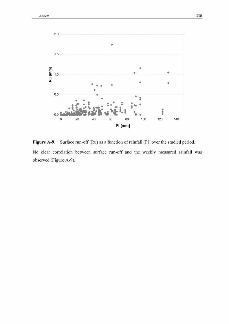
Annex 330
0.0
0.5
1.0
1.5
2.0
0 20 40 60 80 100 120 140
Pi [mm]
Ru [m
m]
Figure A-9. Surface run-off (Ru) as a function of rainfall (Pi) over the studied period.
No clear correlation between surface run-off and the weekly measured rainfall was
observed ( Figure A-9).

Annex 331
ANNEX 5 LINEAR REGRESSIONS AMONG THE MEASURED SOIL MOISTURES
Table A-12 Intercepts, slopes and R-square of the linear regressions relating the water contents measured for a given TDR probe to the average water content for all probes of the experiment.
Treatment Repetition Intercept (%) Slope R-square BCF1 BCF2 CFP AP
1 -1.98 -1.74 -1.58 -1.51 1.05 0.96
2 -0.22 -1.07 -1.26 -0.33 1.09 0.96
3 -0.83 -1.19 -0.93 -1.63 0.91 0.90 1
All -1.01 -1.33 -1.26 -1.16 1.02 0.99
1 -0.83 -0.34 -0.23 -0.92 1.00 0.93
2 4.78 4.68 4.15 4.12 0.90 0.90
3 2.11 2.93 2.62 1.21 0.88 0.80 3
All 2.02 2.42 2.18 1.47 0.92 0.97
1 -4.81 -4.95 -4.44 -3.40 1.06 0.93
2 -1.54 -1.20 -1.56 -1.40 1.10 0.97
3 3.34 2.89 3.23 3.87 1.01 0.89
15 c
m
5
All -1.01 -1.09 -0.92 -0.31 1.06 0.98
1 -1.20 -0.74 -0.75 -0.59 1.04 0.98
2 0.62 -1.27 -0.98 -0.05 1.07 0.96
3 -0.35 -0.45 -0.55 -0.24 0.96 0.98 1
All -0.31 -0.82 -0.76 -0.29 1.02 0.99
1 1.97 2.67 2.56 1.73 0.93 0.98
2 2.06 1.53 1.37 0.62 1.02 0.97
3 1.00 1.68 1.60 1.35 0.90 0.91 3
All 1.68 1.96 1.84 1.23 0.95 0.98
1 -2.33 -1.39 -1.37 -1.25 0.98 0.97
2 -1.21 -0.98 -0.88 -0.52 1.02 0.98
3 -0.57 -1.05 -1.00 -1.05 1.08 0.92
50 c
m
5
All -1.37 -1.14 -1.08 -0.94 1.03 0.99
1 -2.07 -2.16 -2.49 -2.88 1.13 0.97
2 2.40 1.83 1.75 0.10 0.88 0.98
3 -0.45 -1.10 -1.12 -1.74 1.04 0.94 1
All -1.03 -1.68 -1.87 -2.13 1.08 0.98
1 1.17 1.13 1.13 1.58 0.95 0.95
2 -0.76 -1.09 -0.85 -1.18 1.08 0.99
3 1.06 1.73 1.82 0.51 0.89 0.87 3
All 0.49 0.59 0.70 0.30 0.97 0.99
1 -0.63 0.05 -0.05 0.19 0.97 0.98
2 -0.94 -0.59 -0.33 -0.09 0.98 0.99
3 1.71 2.02 2.02 3.06 0.98 0.96
150
cm
5
All 0.04 0.49 0.55 1.06 0.98 0.99
1 -0.55 -1.00 -1.25 -1.74 1.07 0.93
2 1.45 0.68 0.67 0.46 0.99 0.98
3 -0.51 -1.02 -0.88 -1.10 1.04 0.98 1
All 0.13 -0.45 -0.49 -0.79 1.03 0.98
1 5.28 5.75 5.91 5.99 0.77 0.97
2 -3.47 -3.69 -3.62 -3.71 1.10 0.99
3 -3.67 -3.66 -3.49 0.10 1.10 0.97 3
All -0.13 0.01 0.16 0.30 0.97 0.99
1 2.59 3.24 3.17 3.19 0.87 0.98
2 3.91 4.33 4.19 4.27 0.87 0.99
3 -6.12 -5.83 -5.95 -6.03 1.24 0.97
300
cm
5
All 0.13 0.58 0.47 0.48 0.99 0.99

Annex 332

Annex 333
ANNEX 6 SIMULATED AGAINST MEASURED WATER CONTENTS FOR THE BCF AND CFP PERIODS
15 cm
y = 1.1354x - 2.0736R2 = 0.9148
17
19
21
23
25
17 19 21 23 25
Measured water content (%)
Sim
ulat
ed w
ater
con
tent
(%)
50 cm
y = 0.7454x + 6.4053R2 = 0.896
17
19
21
23
25
17 19 21 23 25
Measured water content (%)
150 cm
y = 0.5927x + 8.8734R2 = 0.549
17
19
21
23
25
17 19 21 23 25
Measured water content (%)
Figure A-10. Simulated against measured volumetric water contents for the CFP period in treatment 3. The intercept, slopes and R-square of the regressions are indicated.
y = 0.89x + 3.72R2 = 0.75
10
15
20
25
30
10 15 20 25 30
Sim
ulat
ed w
ater
con
tent
(%)
y = 0.87x + 4.49R2 = 0.79
10
15
20
25
30
10 15 20 25 30
Measured water content (%)
Sim
ulat
ed w
ater
con
tent
(%)
y = 0.72x + 5.88R2 = 0.76
10
15
20
25
30
10 15 20 25 30
y = 0.69x + 8.21R2 = 0.83
10
15
20
25
30
10 15 20 25 30
Measured water content (%)
y = 0.75x + 4.29R2 = 0.91
10
15
20
25
30
10 15 20 25 30
y = 0.66x + 8.02R2 = 0.74
10
15
20
25
30
10 15 20 25 30
Measured water content (%)
BCF2
BCF1
15 cm 50 cm 150 cm
Figure A-11. Simulated against measured volumetric water contents for the BCF period in treatment 3. The intercept, slopes and R-square of the regressions are indicated.

Annex 334

Annex 335
ANNEX 7 CUMULATIVE FLUXES FROM CLEAR FELLING UNTIL THE END OF THE EXPERIMENTAL PERIOD
Table A-13 Average cumulative fluxes and standard deviations (when n≥3) calculated from the clear felling (Nmonth=9) to the end of the experimental period (Nmonth=37) for cations and anions measured in soil solutions for each collector type, collection depth and treatment.
Treatment Cl NO3 NO2 NH4 SO4 PO4 H Na K Mg Ca nobs Fe Al Si DOC mmol m-2 mmol m-2 g m-2
Rainfall 57 39 3 45 14 1 18 23 17 11 22 1 0 0 8 4 Throughfall 1 29 (4) 21 (0) 2 (0) 20 (2) 7 (0) 0 (0) 7 (0) 13 (1) 19 (2) 9 (1) 15 (2) 3 0 1 2 7 3 24 (2) 21 (1) 2 (0) 22 (1) 7 (1) 1 (0) 7 (0) 10 (1) 15 (1) 9 (0) 15 (1) 3 0 1 2 7 5 40 (6) 20 (0) 2 (0) 23 (1) 8 (0) 1 (0) 9 (1) 13 (1) 26 (6) 9 (0) 18 (1) 3 0 1 3 8 Stemflow 1 3 (1) 0 (0) 0 (0) 0 (0) 0 (0) 0 (0) 0 (0) 1 (0) 1 (1) 1 (0) 0 (0) 3 0 0 0 0
3 2 (1) 0 (0) 0 (0) 0 (0) 0 (0) 0 (0) 0 (0) 1 (0) 1 (0) 0 (0) 0 (0) 3 0 0 0 0 5 3 (1) 0 (0) 0 (0) 0 (0) 0 (0) 0 (0) 0 (0) 1 (0) 1 (1) 0 (0) 0 (0) 3 0 0 0 0
Zero-tension lysimeter
0 cm 1 227 (50) 56 (15) 14 (3) 49 (34) 23 (3) 2 (1) 11 (10) 78 (16) 177 (56) 235 (75) 174 (52) 3 7 18 30 79 3 321 (130) 55 (14) 13 (6) 382 (182) 210 (69) 7 (6) 40 (42) 114 (21) 235 (113) 225 (52) 182 (35) 3 14 27 33 91 5 334 (91) 103 (77) 16 (9) 352 (224) 231 (169) 10 (6) 72 (22) 140 (115) 235 (59) 84 (22) 136 (42) 3 29 34 43 76
15 cm 1 111 (30) 197 (46) 2 (0) 23 (9) 16 (4) 1 (0) 117 (28) 57 (25) 47 (8) 59 (7) 36 (18) 3 3 67 90 24 3 191 (97) 267 (70) 6 (3) 184 (187) 315 (335) 19 (31) 204 (14) 96 (61) 101 (33) 100 (26) 93 (73) 3 3 103 117 31
5 268 (55) 604 (181) 7 (2) 362 (178) 288 (62) 1 (0) 255 (8) 65 (8) 98 (32) 64 (9) 98 (17) 3 4 264 157 21 Tension lysimeter
15 cm 1 343 (214) 334 (84) 4 (3) 19 (16) 41 (34) 1 (1) 83 (16) 150 (66) 106 (61) 81 (55) 66 (45) 3 0 109 311 15 3 155 (64) 468 (166) 3 (2) 131 (187) 331 (162) 96 (164) 118 (5) 156 (59) 79 (26) 125 (22) 265 (290) 3 0 147 313 18 5 393 (191) 550 (165) 5 (2) 24 (25) 79 (67) 2 (2) 128 (25) 87 (11) 203 (145) 48 (13) 66 (30) 3 0 229 267 11
50 cm 1 387 (190) 355 (105) 1 (1) 104 (147) 13 (10) 0 (0) 85 (23) 164 (35) 109 (50) 37 (3) 30 (1) 3 0 153 240 7 3 142 (100) 410 (84) 2 (1) 101 (159) 87 (134) 1 (2) 69 (13) 117 (82) 45 (31) 51 (26) 67 (49) 6 0 136 220 8 5 221 (195) 679 (236) 2 (1) 8 (6) 6 (6) 0 (0) 108 (37) 60 (31) 111 (180) 30 (7) 38 (12) 6 0 238 294 5
100 cm 1 645 (528) 281 (104) 1 (0) 97 (136) 2 (1) 0 (0) 74 (19) 98 (24) 216 (257) 25 (3) 28 (4) 3 0 157 208 5 3 126 (213) 368 (242) 1 (1) 45 (74) 3 (6) 0 (0) 46 (13) 154 (164) 26 (27) 28 (13) 30 (10) 12 0 79 158 5 5 156 (91) 416 (124) 5 (2) 5 (3) 1 (0) 0 (0) 80 (24) 71 (17) 39 (33) 26 (8) 28 (8) 3 0 159 160 4
300 cm 1 17 (7) 38 (21) 0 (0) 4 (3) 0 (0) 0 (0) 8 (4) 21 (4) 5 (1) 7 (2) 13 (7) 3 0 15 83 3 3 10 (4) 24 (12) 1 (0) 4 (8) 0 (0) 0 (0) 5 (2) 12 (6) 3 (1) 4 (2) 8 (3) 12 0 1 66 1 5 13 (5) 56 (23) 1 (0) 6 (4) 0 (0) 0 (0) 15 (3) 56 (85) 4 (1) 6 (1) 17 (9) 6 0 4 84 2


Annex 337
ANNEX 8 SPECIFIC EXTRACTIONS PERFORMED ON SOILS AT AGE 2 YEARS AFTER PLANTING
Table A-14 Specific extractions performed on soils at age 2 years after planting: reference stand kept uncut. Mean and standard errors (when n≥3) are given. Reference 0-5 cm 5-15 cm 15-30 cm 30-50 cm 50-100 cm 100-200 cm 200-300 cm
Water extraction on fresh soil Ca 1 0.2 1 0.0 1 0.1 2 0.2 5 1.3 9 1.1 11 0.4
Mg 0 0.0 0 0.0 1 0.0 1 0.2 1 0.1 3 0.6 4 0.4 Na 1 0.0 2 0.3 3 0.2 3 0.2 11 0.8 17 3.9 25 0.8 H 0 0.0 1 0.0 1 0.0 1 0.1 2 0.2 5 0.7 6 0.3
Al 5 2.3 13 3.4 12 6.5 5 2.5 9 7.4 1 0.4 1 0.7 N/NH4 1 0.1 1 0.2 1 0.4 1 0.4 4 0.3 6 0.8 9 1.3 N/NO3 1 0.2 1 0.3 1 0.3 1 0.1 4 1.7 9 2.4 28 3.8 S/SO4
kg ha-1
0 0.1 2 0.3 3 0.6 5 0.7 4 0.7 4 0.3 5 0.6
KCl extraction on fresh soil N/NO3 1 0.1 1 0.1 0 0.0 0 0.0 2 0.1 4 1.0 12 2.6 N/NH4
kg ha-1 1 0.0 1 0.1 2 0.3 2 0.3 4 0.2 6 1.0 8 1.1
KCl extractions (except for K, NH4Cl extraction) (air-dry soil) K 15 1.5 15 1.1 13 0.8 13 3.0 22 4.5 32 3.3 34 4.0
Ca 7 2.0 14 2.3 17 7.5 9 8.8 44 12.6 144 41.2 145 49.2 Mg 2 0.5 3 0.3 2 0.5 0 0.5 5 4.9 15 8.8 8 4.6 Na 0 0.0 0 0.0 0 0.0 0 0.0 93 93.1 328 167.7 74 74.3 H 4 1.1 1 0.0 2 0.1 1 0.7 2 0.9 6 0.1 0 0.0
Al
kg ha-1
159 23.5 167 6.7 226 7.7 229 5.7 420 21.8 628 23.8 169 7.4 Saturation cmolc/kg 0.3 0.05 0.1 0.01 0.1 0.02 0.1 0.02 0.1 0.01 0.1 0.02 0.1 0.02
CEC cmolc/kg 2.7 0.37 1.2 0.01 1.0 0.01 0.5 0.22 0.4 0.18 0.5 0.02 0.1 0.01 N/NO3 2 0.6 3 1.6 3 0.2 4 0.9 15 3.7 30 11.8 87 28.1
S (total) 49 10.1 88 4.3 170 13.0 210 8.0 349 77.1 786 101.8 451 99.4 P (total)
kg ha-1 5 0.5 10 1.5 17 3.0 17 0.1 45 8.3 99 7.2 90 0.3
Specific extractions S/SO4 4 0.9 9 1.4 22 9.1 12 1.2 15 5.5 24 5.0 24 9.0 P/PO4
kg ha-1 2 0.3 1 0.0 1 0.1 2 0.1 1 0.3 3 1.0 3 0.0

Annex 338
Table A-15 Specific extractions performed on soils at age 2 years after planting: Treatment 1. Mean and standard errors (when n≥3) are given. Treatment 1 0-5 cm 5-15 cm 15-30 cm 30-50 cm 50-100 cm 100-200 cm 200-300 cm
Water extraction on fresh soil Ca 1 0.3 2 0.3 2 0.1 3 0.7 5 12 10 1
Mg 0 0.2 1 0.1 1 0.0 1 0.0 2 4 3 0Na 2 0.1 4 0.5 5 0.9 6 0.5 17 32 34 2H 0 0.0 0 0.1 1 0.2 1 0.1 1 4 2 0
Al 14 3.4 37 5.2 26 6.9 10 4.4 2 2 1 14N/NH4 1 0.1 0 0.2 0 0.2 1 0.1 2 7 6 1N/NO3 0 0.1 0 0.2 1 0.1 1 0.5 1 2 10 0S/SO4
kg ha-1
1 0.1 2 0.2 4 0.7 6 1.2 3 3 3 1
KCl extraction on fresh soil N/NO3 0 0.1 0 0.0 0 0.1 0 0.0 1 2 4 0N/NH4
kg ha-1 2 0.3 1 0.2 2 0.5 1 0.1 6 13 6 2
KCl extractions (except for K, NH4Cl extraction) (air-dry soil) K 14 1.2 13 0.8 13 1.5 11 1.2 15 114 15 14
Ca 73 29.9 13 8.3 4 4.3 9 8.6 0 0 65 73Mg 42 15.7 9 2.6 5 2.3 5 2.4 9 20 31 42Na 0 0.0 0 0.0 0 0.0 10 9.9 0 0 86 0H 2 0.9 2 0.4 2 0.3 2 0.1 2 4 0 2
Al
kg ha-1
92 25.6 127 9.6 174 10.4 206 9.8 321 400 81 92Saturation cmolc/kg 1.3 0.45 0.2 0.06 0.1 0.03 0.1 0.02 0.0 0.0 0.1
CEC cmolc/kg 3.0 0.24 1.2 0.15 1.0 0.08 0.9 0.02 0.6 0.4 0.2 N/NO3 2 0.3 2 0.7 2 1.6 4 0.8 12 3 47 2
S (total) 23 4.4 41 6.2 68 10.1 122 4.3 122 163 209 23P (total)
kg ha-1 2 0.6 5 1.5 8 2.7 12 4.8 8 19 20 2
Specific extractions S/SO4 3 1.2 4 0.5 12 5.9 14 1.4 0 0 0 3P/PO4
kg ha-1 2 0.3 24 9.7 3 0.8 2 0.4 2 4 13 2

Annex 339
Table A-16 Specific extractions performed on soils at age 2 years after planting: Treatment 3. Mean and standard errors (when n≥3) are given. Treatment 3 0-5 cm 5-15 cm 15-30 cm 30-50 cm 50-100 cm 100-200 cm 200-300 cm
Water extraction on fresh soil Ca 1 0.2 2 0.3 3 0.7 3 0.8 7 2.1 13 2.4 10 1.4
Mg 1 0.4 2 0.5 2 0.5 2 0.5 4 2.2 7 3.2 4 0.6 Na 2 0.2 4 0.5 5 0.8 6 1.3 14 1.2 29 3.8 24 2.6 H 0 0.0 1 0.1 1 0.1 2 0.2 3 0.3 7 0.6 4 1.0
Al 13 7.2 17 3.7 11 3.1 3 1.0 5 2.9 5 2.1 2 0.3 N/NH4 0 0.2 1 0.4 1 0.0 1 0.1 6 2.8 9 2.9 7 0.6 N/NO3 0 0.1 0 0.2 0 0.2 1 0.4 3 1.9 29 11.4 18 5.1 S/SO4
kg ha-1
2 0.6 6 1.9 13 2.3 26 7.6 20 0.7 5 0.7 5 0.6
KCl extraction on fresh soil N/NO3 0 0.0 0 0.0 0 0.0 0 0.0 3 1.0 15 7.5 9 2.9 N/NH4
kg ha-1 1 0.1 1 0.1 1 0.3 1 0.5 7 3.7 7 2.1 7 1.7
KCl extractions (except for K, NH4Cl extraction) (air-dry soil) K 19 4.9 77 63.5 12 2.2 12 1.9 60 39.8 35 28.7 10 6.3
Ca 71 19.0 8 1.9 19 18.3 3 2.3 4 4.4 16 16.4 55 32.0 Mg 55 12.3 14 1.7 8 1.6 6 1.5 10 10.2 12 12.2 4 4.3 Na 1 1.0 0 0.0 2 2.2 0 0.0 0 0.0 0 0.0 12 12.2 H 4 1.9 2 0.2 3 0.2 2 0.1 3 0.1 5 0.8 0 0.0
Al
kg ha-1
121 45.4 143 20.1 207 15.9 251 12.1 423 27.1 531 54.8 148 36.3 Saturation cmolc/kg 1.5 0.31 0.3 0.12 0.1 0.04 0.1 0.01 0.1 0.01 0.0 0.01 0.0 0.01
CEC cmolc/kg 3.8 0.90 1.4 0.15 1.1 0.10 0.9 0.07 0.7 0.02 0.4 0.03 0.0 0.01 N/NO3 1 0.3 1 0.1 1 0.3 3 1.0 11 3.5 81 32.4 62 18.2
S (total) 37 3.0 77 14.2 195 12.6 402 84.4 546 14.3 298 57.9 262 65.8 P (total)
kg ha-1 4 1.4 7 2.4 7 2.8 9 3.5 23 10.8 44 22.0 47 27.7
Specific extractions S/SO4 7 0.8 14 4.4 27 7.1 64 22.5 71 15.9 6 5.6 0 0.0 P/PO4
kg ha-1 4 1.2 11 9.1 17 15.6 1 0.1 2 0.6 20 14.3 19 15.4

Annex 340
Table A-17 Specific extractions performed on soils at age 2 years after planting: Treatment 5. Mean and standard errors (when n≥3) are given. Treatment 5 0-5 cm 5-15 cm 15-30 cm 30-50 cm 50-100 cm 100-200 cm 200-300 cm
Water extraction on fresh soil Ca 1 0.1 2 0.2 3 0.6 3 0.1 5 14 12
Mg 0 0.0 1 0.0 1 0.1 1 0.1 2 6 5 Na 2 0.2 3 0.4 6 2.1 5 1.1 15 24 29 H 0 0.1 1 0.0 2 0.4 1 0.1 2 8 6
Al 12 4.3 4 2.5 14 8.0 6 2.1 11 5 5 N/NH4 0 0.2 1 0.3 2 0.7 3 0.7 9 19 17 N/NO3 0 0.2 1 0.1 1 0.1 1 0.1 1 46 43 S/SO4
kg ha-1
1 0.2 7 0.8 13 3.8 12 1.0 13 7 6
KCl extraction on fresh soil N/NO3 0 0.0 0 0.0 0 0.1 0 0.1 1 31 0 0N/NH4
kg ha-1 1 0.2 1 0.1 2 0.4 2 0.3 4 8 10 1
KCl extractions (except for K, NH4Cl extraction) (air-dry soil) K 15 1.9 13 0.5 11 0.6 8 1.4 17 21 8 15
Ca 23 3.6 1 0.6 3 3.1 4 2.1 86 0 3 23Mg 5 1.0 1 0.1 3 2.0 2 1.7 36 9 19 5Na 0 0.0 0 0.0 0 0.0 0 0.0 448 0 0 0H 3 0.7 2 0.2 8 5.3 2 0.8 5 6 0 3
Al
kg ha-1
118 31.0 167 1.0 227 3.9 226 5.4 377 500 137 118Saturation cmolc/kg 0.4 0.03 0.1 0.01 0.1 0.02 0.2 0.13 0.1 0.0 0.0
CEC cmolc/kg 2.4 0.41 1.2 0.02 1.1 0.06 1.0 0.20 0.8 0.5 0.0 N/NO3 2 0.3 2 0.2 3 1.0 4 1.3 24 66 92 2
S (total) 42 9.7 141 26.7 238 71.3 221 38.9 281 21 0 42P (total)
kg ha-1 3 1.5 8 2.9 9 3.9 11 6.7 11 23 40 3
Specific extractions S/SO4 5 0.4 17 1.8 30 9.0 28 3.9 22 0 0 5P/PO4
kg ha-1 7 2.9 1 0.1 2 0.0 1 0.1 20 6 9 7

341
ARTICLE


Article 343
Influence of land use (savanna, pasture,Eucalyptus plantations) on soil carbon andnitrogen stocks in Brazil
V. MAQUEREa,b , J. P. LACLAU
b,d , M. BERNOUXc , L. SAINT-ANDRE
b , J. L. M. GONCxALVESd ,
C. C. CERRIe , M. C. PICCOLO
e & J. RANGERf
aENGREF, 19 av. du Maine, 75732 Paris Cedex 15, France, bCIRAD, UPR80, TA 10/D, 34398 Montpellier Cedex 5, France,cIRD, UR SeqBio, SupAgro – Batiment 12, 2 place Viala, 34060 Montpellier Cedex 1, France, dDepartment of Forest Sciences, ESALQ/
USP, Piracicaba, SP, Brazil, eLaboratorio de Biogeoquımica Ambiental, CENA/USP, Piracicaba, SP, Brazil, and fINRA Centre de Nancy,
Biogeochimie des Ecosystemes Forestiers, 54280 Champenoux, France
Summary
In Brazil, most Eucalyptus stands have been planted on Cerrado (shrubby savanna) or on Cerrado con-
verted into pasture. Case studies are needed to assess the effect of such land use changes on soil fertility
and C sequestration. In this study, the influence of Cerrado land development (pasture and Eucalyptus
plantations) on soil organic carbon (SOC) and nitrogen (SON) stocks were quantified in southern Bra-
zil. Two contrasted silvicultural practices were also compared: 60 years of short-rotation silviculture
(EUCSR) versus 60 years of continuous growth (EUCHF). C and N soil concentrations and bulk densi-
ties were measured and modelled for each vegetation type, and SOC and SON stocks were calculated
down to a depth of 1 m by a continuous function.
Changes in SOC and SON stocks mainly occurred in the forest floor (no litter in pasture and up to 0.87 kg
C m�2 and 0.01 kg N m�2 in EUCSR) and upper soil horizons. C and N stocks and their confidence
intervals were greatly influenced by the methodology used to compute these layers. C/N ratio and 13C
analysis showed that down to a depth of 30 cm, the Cerrado organic matter was replaced by organic mat-
ter from newly introduced vegetation by as much as 75–100% for pasture and about 50% for EUCHF,
poorer in N for Eucalyptus stands (C/N larger than 18 for Eucalyptus stands). Under pasture, 0–30 cm
SON stocks (0.25 kg N m�2) were between 10 and 20% greater than those of the Cerrado (0.21 kg N
m�2), partly due to soil compaction (limit bulk density at soil surface from 1.23 for the Cerrado to 1.34
for pasture). Land development on the Cerrado increased SOC stocks in the 0–30 cm layer by between 15
and 25% (from 2.99 (Cerrado) to 3.86 (EUCSR) kg C m�2). When including litter layers, total 0–30 cm
carbon stocks increased by 35% for EUCHF (4.50 kg C m�2) and 53% for EUCSR (5.08 kg C m�2),
compared with the Cerrado (3.28 kg C m�2), independently of soil compaction.
Introduction
Organic matter (OM) is an essential component for soil fertility:
it is a direct source of nutrients and contributes to cation reten-
tion, soil structure and biological activity. Soil organic nitrogen
(SON) is essential because nitrogen is involved in numerous
physiological functions and is themost abundantly accumulated
nutrient in plant biomass (Marschner, 1995). As for soil organic
carbon (SOC), the present debate on climate change has high-
lighted the importance of high soil C storage capacity that is still
poorly quantified at this time (Intergovernmental Panel on
Climate Change, 2001). Organic matter is essential in tropical soils
where primary minerals have generally been totally depleted
(Feller & Beare, 1997). To exemplify this, wood production in
tropical Eucalyptus plantations planted on poor soils has been
shown to be dependent on the amount of organic matter left on-
site when the former stand was harvested (Nambiar et al., 2004).
In Brazil, Eucalyptus plantations have been introduced since
the beginning of the 20th century on more than three million
hectares and obtain high yields (typically, 40–50 m3 ha�1
year�1). Their management can greatly modify soil chemical
and physical properties (Goncxalves et al., 2004). It was observed
in the Congo that long-term silviculture of Eucalyptus led toCorrespondence: V. Maquere. E-mail: [email protected]
Received 4 May 2007; revised version accepted 29 May 2008
European Journal of Soil Science, October 2008, 59, 863–877 doi: 10.1111/j.1365-2389.2008.01059.x
# 2008 The Authors
Journal compilation # 2008 British Society of Soil Science 863

Article 344
imbalanced N budgets (Laclau et al., 2005), which can result in
SON impoverishment. The quantification of SOC and SON
changes is thus essential to assess the long-term impact of Euca-
lyptus plantations on soil fertility compared with more tradi-
tional land uses (Cerrado and pasture in Brazil).
In theAmazon, SOC stocks were estimated in primitive forest
on the regional scale (Moraes et al., 1995; Bernoux et al., 1998a,
2002). Other studies were conducted in Brazil on the plot scale
when native vegetation (Cerrado or primitive forest) was con-
verted to pasture or crops (Moraes et al., 1996; Bernoux et al.,
1998c; De Freitas, 2000; Cerri et al., 2004; Corbeels et al.,
2006). However, little information is available concerning the
impact of pine (Smith et al., 2002; Lilienfein & Wilcke, 2003)
and Eucalyptus plantations (Lepsch, 1980; Zinn et al., 2002;
Lima et al., 2006) on SOC and SON stocks. Moreover, one
possible option for increasing carbon sequestration in tropical
forest plantations (clean development mechanisms) discussed
in post-Kyoto meetings would be to lengthen rotation time.
The influence of this silvicultural scenario on SOC and SON
stocks has not yet been studied in Brazilian Eucalyptus
plantations.
This study aimed at: (i) quantifying, on a hectare basis, the
influence of different Cerrado land developments (pasture ver-
sus Eucalyptus plantations) on SOC and SON stocks, 20 and
60 years after land use change; (ii) assessing the influence of
contrasted silvicultural practices (60 years of continuous
growth versus short-rotation silviculture over 60 years) on
SOC and SON storage; (iii) quantifying the effect of soil com-
paction on SOC and SON stocks; and (iv) modelling SOC and
SON stocks down to a depth of 1 m using a continuous func-
tion for each land use.
Material and methods
Experimental area
The study was conducted at the experimental station of Sao
Paulo University, Itatinga, Brazil (23°02¢S, 48°38¢W). The cli-
mate is Cfa according to the Koppen classification. The aver-
age annual precipitation was 1370 mm and the average annual
temperature was 19.2°C from 1990 to 2004.
The relief is typical of the Sao Paulo Western Plateau, with
topography varying from flat to hilly (FAO, 1977). The maxi-
mum altitude is 860 m. The lithology is a Cretaceous sandstone
belonging to the Marılia formation and the Bauru group.
Soil spatial distribution is organized according to altitude and
slope. Sampled plant communities are located on ‘latosolos ver-
melhos amarelos distroficos typicos A’, according to the Brazil-
ian classification (EMBRAPA, Centro Nacional de Pesquisa de
Solos, 1999), and Ferralsols, according to the FAO classifica-
tion. Preliminary geomorphological studies showed that their
occurrence at the Itatinga Experimental Station corresponded
to altitudes > 800 m and slopes < 10%.
Sampled vegetation types (VT)
Soils were sampled under five plant communities: a prevailing
shrub and tree savanna known as Cerrado (CER) in Brazil,
a pasture established on this Cerrado 20 years ago (PAS20),
a pasture established on this Cerrado 80 years ago (PAS80),
a 60-year-old Eucalyptus saligna Smith stand managed in short
rotations of 6–10 years (EUCSR), and a 60-year-old Eucalyptus
saligna high forest (EUCHF). The dominant species of both
pastures is Brachiaria. The dominant species of the plant com-
munities sampled are given in Maquere, 2004. Both Eucalyptus
stands were planted between 1941 and 1944 on 20-year-old
pastures, previously established on the same Cerrado. For all
vegetation types (VT), the slope was less than 10% (Table 1).
Emphasis was placed on choosing sites whose historywaswell
known (from 60 years ago to today), that presented homoge-
nous ecological conditions (soil, geology, topography). Such
sites were scarce because 60-year-old Eucalyptus high forests
are quite exceptional in Brazil. One site for each vegetation
type was found within a 2-km-radius area (Figure 1). The soil
spatial heterogeneity within and between vegetation types was
then carefully studied (see below) to make sure that SOC and
SON stock variations resulted from land use change and not
from differences in ecological conditions.
Table 1 Characteristics of the five studied vegetation types
Vegetation type (VT) Abbreviation Vegetation Slope/° Management
Cerrado CER Shrubs and Graminaceae 4 Casual extensive pasture
20-year-old pasture PAS20 Brachiaria 7 Extensive pasture
80-year-old pasture PAS80 Brachiaria 6 Extensive pasture
Eucalyptus short-rotation
management since 1944
EUCSR Eucalyptus saligna 1 Coppice management from 1944 to 1997: 6–10 year-long
rotations, no fertiliser input
Site replanted in 1998 with 1667 trees ha�1 density.
Fertilisation at planting: 300 kg ha�1 NPK 10:20:10
Chemical weeding (glyphosate) the first year after planting
Eucalyptus high forest planted in 1944 EUCHF Eucalyptus saligna 1 Casual local thinning
864 V. Maquere et al.
# 2008 The Authors
Journal compilation # 2008 British Society of Soil Science, European Journal of Soil Science, 59, 863–877

Article 345
Sampling
In each VT, three plots were positioned along a 100-m long
transect going down the slope. Each plot was composed of five
40-cm deep pits, plus one 100-cm deep soil pit. All in all, 18 pits
were sampled in each vegetation type (Figure 1). Soils were sam-
pled with a 10-cm diameter corer at depths of 0–5 cm, 5–10 cm,
10–20 cm, 20–30 cm and 30–40 cm, plus 40–60 cm, 60–80 cm
and 80–100 cm for the 100–cm deep soil pits. Sampling was
performed at a fixed depth since no clear limit between soil hori-
zons could be observed.
Soils were oven dried at 40°C, passed through a 2-mm mesh,
and an aliquot was ground to 150 mm for carbon and nitrogen
determination (LECO analyser). Individual analyses were per-
formed for each sample collected. A soil aliquot was dried at
105°C for residual humidity and bulk density determinations.
Individual bulk density was measured for each sample in order
to avoid any systematic error due to the use of an average bulk
density (Arrouays et al., 2003).
Litter (L1) was sampled in each vegetation type with a 30-cm
diameter metal ring at 1 m from each pit. For EUCHF, the litter
sampling scheme needed to be adapted: a supplementary layer
(L2) made of charcoal, sand and a dense root material that
adhered to decomposed OM was observed between the fresh
litter layer and the mineral soil. Such a litter structure had
already been observed in Congolese Eucalyptus plantations
(Laclau et al., 2004). This layer was sampled for each pit,
whenever present, using a 225-cm2 frame, and its thickness
was measured. Litter and roots were dried at 65°C. L1 litter
was divided into four fractions (bark, branch, leaf and mis-
cellaneous), each fraction was weighed, and one composite
sample per fraction and per plot was ground for C and N
determination. L2 litter was divided into three fractions: char-
coal, roots and pieces of vegetal matter > 2mm, and mineral
and organic particles < 2 mm. Each fraction was weighed and
then ground for C and N determination.
Soil parent material homogeneity between and within
vegetation types
Preliminary studies showed that the soils of the sampled region
were spatially distributed according to topography and differed
by their particle size distribution and mineralogy (EMBRAPA,
Centro Nacional de Pesquisa de Solos, 1999). These character-
istics, little affected by land use in deep soil horizons, were
chosen to check the homogeneity of the soil parent material.
A particle-size analysis and a pedological description were
performed in each vegetation type for a whole profile down to
a depth of 1 m. For particle size distribution, differences among
VT were expected to occur in the accumulation horizon, i.e.
beyond a depth of 40 cm (EMBRAPA, Centro Nacional de
Pesquisa de Solos, 1999). Soil layers deeper than 40 cm were
thus considered as a unique layer, and their corresponding
particle size distribution values were taken as a unique data set
for each VT.
For three pits per vegetation type, a mineralogical analysis
was performed by X-ray diffraction on soil samples collected
in the 80–100 cm layer. The X-ray diffractometer was a Siemens
D5000 (Siemens AG, Munich, Germany) equipped with a Cu
anticathode and a graphite monochromator (30 mA and
40 KeV). The rotation speed was 0.02° s�1 (absolute). The dif-
fractograms were performed on powder made from the whole
soil.
13C measurements
In each vegetation type, d13C was measured down to a depth of
1 m for one soil profile and its corresponding L1 and/or L2 lit-
ter samples. One composite sample consisting of ground roots
dried at 65°C was also analysed for each VT. The isotopic
composition of soil organic matter closely resembles the iso-
topic composition of the vegetation from which it is derived
because the fractionation during decomposition is small rela-
tive to the original fractionation during C fixation (Peterson &
Fry, 1987; Nadelhoffer & Fry, 1988; Bernoux et al., 1998c).
When one type of vegetation is replaced by another, d13C val-
ues can be used to identify soil OM derived from the original
vegetation residues (Cerrado) or from the new vegetation resi-
dues. The C content of each component is given by Cerri et al.
(1985), Bernoux et al. (1998c) and Wilcke & Lilienfein (2004):
CVTðxÞ ¼ COriginalðxÞ þ CVegðxÞ; ð1Þ
CVegðxÞ ¼ QVegðxÞ � CVTðxÞ; ð2Þ
COriginalðxÞ ¼ QOriginalðxÞ � CVTðxÞ¼ ð1 � QVegðxÞÞ � CVTðxÞ;
ð3Þ
Figure 1 Localization of each sampled vegetation type (a) and sampling
design used in each one of them (b) CER ¼ Cerrado; EUCSR ¼60-year-old Eucalyptus saligna Smith stand managed in short rotations;
EUCHF ¼ 60-year-old Eucalyptus saligna high forest; PAS20 ¼ pasture
installed on the Cerrado 20 years ago; PAS80 ¼ pasture installed on the
Cerrado 80 years ago.
Land use influence on soil C&N stocks in Brazil 865
# 2008 The Authors
Journal compilation # 2008 British Society of Soil Science, European Journal of Soil Science, 59, 863–877

Article 346
QVegðxÞ ¼d13CVTðxÞ � d13CCER
d13CVegðxÞ � d13CCER
; ð4Þ
where CVT(x) is the C concentration function in % measured
at depth x in vegetation type VT. QOriginal(x) and COriginal(x)
are the C fraction and the C concentration in % taken from
the C pool before the land use change, and QVeg(x) and CVeg(x)
are the C fraction and the C concentration in % taken from
the present vegetation type at depth x. d13CVT(x) is the d13C
measured at depth x in the vegetation type VT, d13CCER(x) is
the d13C measured in the Cerrado at the same depth x, and
d13CVeg is the d13C signature of the fresh organic matter input
of the present vegetation and was taken as the average litter
and root d13C values for each vegetation type (Bernoux et al.,
1998c). Differences in the d13C signature were considered sig-
nificant if greater than 1&.
Calculations
Carbon and nitrogen concentration profiles. A preliminary
analysis showed that C and N concentrations were quite sim-
ilar for all VT beyond a depth of 40 cm. An adaptation of the
classical exponential decay type equation was thus chosen to
model C and N vertical distribution, inspired from the model
used by Arrouays and Pelissier (1994) and Bernoux et al.
(1998b).
Model 1 fVTðxÞ ¼ a þ bVT exp ð�cVTxÞ; ð5Þ
bVT ¼ a � fVTðx < 5Þexp ð �ðx < 5ÞcVTÞ
ð6Þ
where f is the C or N concentration function in %, and x is the
depth in cm. VT is a label for the vegetation type. The
a parameter is the asymptotic depth limit concentration
(x/N) fitted in common to all vegetation types, in other
words, it is constant within a given ecological region (global),
a þ bVT is the concentration on the surface (x ¼ 0), bVT is an
input variable obtained from solving Equation 2 for the limit
condition on the surface x 2 fx< 5g, ðx< 5Þ is the average
x 2 fx< 5g, and fVTðx< 5Þ is the average fVTðxÞ 2 ffVTðx< 5Þg(for each VT), bVT is vegetation type-dependent within a given
ecological region (local) and can be easily obtained from soil
measurements, and cVT is the exponential decrease rate for
each VT and is the only parameter dependent of vegetation
type to be fitted.
Bulk density profiles. Preliminary studies showed that bulk
densities were quite similar for all VT beyond a depth of
40 cm. Bulk density profiles were thus modelled using a qua-
dratic polynomial equation whose depth limit value was the
same for all vegetation types:
Model 2 dVTðxÞ ¼ aVT þ bVT x � g2VTx2; if x < 40 cm
ð7Þ
dVTðxÞ ¼ d; if x � 40 cm ð8Þ
bVT ¼ d � aVT40
þ 40 g2VT; ð9Þ
where dVT is the bulk density, x the depth in cm, bVT is derived
from dVT(40) to complete the model continuity for x ¼ 40 cm
(dVT(40) ¼ d), and aVT and gVT are the parameters to be fitted,
aVT is the bulk density on the surface (x/0). The maximum
bulk density is dmax and is reached for a depth xmax, aVT and
gVT are local parameters, whereas d is a global parameter.
Comparison between local and global fits
After building and simplifying, Models 1 and 2 were fitted for
each vegetation type (local models) and for the whole set of data
(global models) using PROC MODEL of SAS software
(www.sas.com). Differences among local and global models
were evaluated from F-tests calculated on the residual. This
test is based on the sums of squares of errors (SSE) and the
total number of parameters involved in the models. It com-
pares Fobs and Ftab calculated as:
Fobs ¼ðSSE2 � SSE1Þ=ðp1 � p2Þ
SSE1=ðn � p1Þ; ð10Þ
where p1 is the number of parameters for the local model, p2 is
the number of parameters for the global model (p2 < p1), SSE1
is the sum of square errors for the local model, SSE2 is the sum
of square errors for the global model, and n is the number of
observations. Ftab is the theoretical value given in the Fischer’s
table Ftab ¼ F(p1�p2,n�p1). If Fobs > Ftab then the local
model described the data set better than the global model and
there was a significant effect of the vegetation type on the
studied function (Brown & Rothery, 1993). All differences
were considered significant at a 5% threshold.
Soil C and N stocks as a function of depth
SOC and SON stocks were calculated by multiplying the C or N
model by the bulk density model and integrating it from 0 to
a fixed depth.
Model 3 SVTðxÞ ¼ðx
0
fVTðmÞdVTðmÞdm; ð11Þ
where SVT is the C or N stock function in kg m�2, x the depth
in m, fVT the C or N concentration function in % obtained
from Model 1 (Equations 5 and 6), and dVT the bulk density
function obtained from Model 2 (Equations 7–9).
866 V. Maquere et al.
# 2008 The Authors
Journal compilation # 2008 British Society of Soil Science, European Journal of Soil Science, 59, 863–877

Article 347
C and N stocks were then computed continuously from the
soil mineral surface down to a depth of 1 m. Confidence inter-
vals (CI) were calculated for these stocks from the following
equation (Parresol, 1999):
S � tð a2 Þ
ffiffiffiffiffiffiffiffiffiffiffiffiffiffiffiffiffiffiffiffiffiffiffiffiffiffiVar2
Sþ s2xk
18
s; ð12Þ
where S is the estimated C or N stock, x is the depth in cm, and
Var2S¼
�@S
@b
�¢
Sb
�@S
@b
�: ð13Þ
Var2Sis the variance of S with @S=@b the derivative matrix of S
with respect to the matrix set of parameters b, ð@S=@bÞ¢ thetranspose matrix of @S=@b, and Sb the covariance matrix of
the model parameter (delta method; Serfling, 1980), s2 is the
estimated variance of the model and xk the estimated weighted
function with k being the optimal exponent for correcting the
data heteroscedasticity. The second term under the square
root s2 Xk=18 stands for the residual variability of the model
spread over the 18 pits considered independently. It contains
the fVTðx< 5Þ surface parameter contribution to the model
variability.
In order to minimize the influence of localized, large C or
N surface concentrations in the 0–5 cm bulk soil layer or
the L2 litter layer for EUCHF (due to charcoal, OM frag-
ments, etc.) on the model parameters, Model 3 was fitted
without these localized C or N concentration points. A
stock profile was then considered to be the sum of two
components (Figure 2): (i) a main component computed
from Model 3 and the fVTðx< 5Þ value of the profile stud-
ied as an input parameter; and (ii) a second component
computed as the measured stock minus its estimated main
component resulting from (i). The average stock for each
VT was obtained by taking the main component from
Model 3 with fVTðx< 5Þ as an input parameter, and the sec-
ond component as the average of the second component
for all 18 pits. For EUCHF, because there was no clear
limit between the L2 litter layer and the mineral soil itself,
the L2 layer (root fraction excluded) was included in the
soil profile and was computed, whenever present, as the
particular points mentioned above (Figure 2).
SOC and SON stocks as a function of soil mass
SOC and SON stock changes can also be assessed independently
of soil compaction. The common stock calculation (Inter-
governmental Panel on Climate Change, 1997) integrates soil
stocks down to a fixed depth, that is, it calculates the stocks
contained in a fixed volume. Changes in stocks may then result
from a soil mass increase (or decrease) in this fixed volume, as
well as from an absolute C or N enrichment (or depletion) of the
volume solid phase itself. This effect can be avoided by integrat-
ing the stocks down to a fixed soil mass instead of to a fixed soil
depth (Ellert et al., 2002).
Figure 2 Organization of litter layers and soil profile whenever litter L2 is present (EUCHF) (A1) or not (A2). Conceptual distribution of total C
and N stock between L1 litter, particular points (L2 litter included), and the bulk soil component of the model (Model 3) for a sampled pit (B)
Note that ðx< 5Þ ¼ 2:5 whenever L2 is not present (soil layers are sampled at fixed depths). In EUCHF, ðx< 5Þ 6¼ 2:5 because L2 is considered part
of the soil profile and its thickness is not necessarily 5.
Land use influence on soil C&N stocks in Brazil 867
# 2008 The Authors
Journal compilation # 2008 British Society of Soil Science, European Journal of Soil Science, 59, 863–877

Article 348
For all vegetation types, the depth intervals were converted to
soil mass based on the bulk density measurements per soil sam-
ple. C and N profiles were modelled as a function of soil mass
using the same exponential decay-type function as in Model 1.
Soil C and N profiles were then:
Model 4 fVTðmÞ ¼ a þ bVT expð �cVTmÞ; ð14Þ
bVT ¼ a � fVTðm< 62Þexp ð �ðm< 62ÞcVTÞ
; ð15Þ
where fVT is the C or N concentration function in %, m is the
soil mass in kg m�2, and a and cVT are the parameters to be
fitted. The average soil mass per unit area of the Cerrado 0–
5 cm bulk soil layer is 62 kg m�2.
The resulting stocks were then calculated as:
Model 5 SVTðmÞ ¼ðm
0
ða þ bVT exp ð �cVTmÞÞdm: ð16Þ
This model is simple to integrate and to fit, and avoids the use of
a complex bulk density model. The confidence intervals were
obtained using the method described above.
Results
Soil parent material homogeneity between and within
vegetation types
For particle-size analysis, differences in clay contents among
vegetation types were less than 5% (Figure 3). They were not
significant at a 5% threshold except for PAS20 and EUCSR,
for which the average clay contents differed by 4%. These dif-
ferences were close to the measurement accuracy.
All vegetation types presented a quasi-identical mineralogical
X-ray signature in their 80–100-cm layer. X-ray spectra showed
the presence of quartz, kaolinite, hematite, goethite and gibbsite.
A non-attributed silicate layer (probably vermiculite) was sug-
gested by a peak that occurred between 2 and 6 degrees 2 h. Itsidentification would have required further analysis. As this sili-
cate was rather scarce, it was not considered within the scope of
this study. It was thus concluded that all vegetation types shared
the same parent material, and that selected sites met the require-
ments for the study.
Litter layers and particular points
Some surface samples (0–5 cm bulk soil layer and the L2 litter
layer) had large C and N concentrations and low bulk densities,
which corresponded to local specificities such as litter remains,
charcoal, pieces of termite mound or ant-hill, and localized OM
accumulation. Such samples were considered as outliers and
were found in EUCSR (seven pits), EUCHF (L2 litter present
for 13 pits), and PAS20 (six pits). For EUCHF, the thickness of
the L2 layer ranged from one to 10 cm, with an average of
3.6 cm. Approximately 90% of its biomass consisted of finely
divided OM (� 1 mm). The C stocks of the second component
of particular points were 0.36 kg C m�2 for EUCHF, 0.35 kg
C m�2 for EUCSR, and 0.03 kg C m�2 for PAS20. These
points accounted for N stocks less than 0.05 kg N m�2
(Table 2).
L1 biomass was greatest for EUCSR and negligible for both
pastures. C litter stocks were greatest for EUCSR (0.87 kg C
m�2), followed by EUCHF (0.46 kg C m�2) and CER (0.29 kg
C m�2). Nitrogen amounts within the forest floor were less
than 0.01 kg N m�2 for all vegetation types (Table 2).
Bulk density
Bulk densities ranged from an average of 1.28 kg dm�3 for the
0–5 cm layer, to an average of 1.38 kg dm�3 for the 80–
100 cm layer. Their depth profiles presented a bump between
a depth of 0 and 40 cm, and remained constant below 40 cm
(Figure 4). F tests showed that Model 2 could be simplified by
fixing the a parameter common to all arboreal formations
(aCER ¼ aEUCHF ¼ aEUCSR) and to both pastures (aPAS20 ¼aPAS80), as well as by fixing the g parameter common to all sit-
uations except for EUCHF (Table 3). As a result, the CER and
EUCSR situations shared common bulk density profiles, as did
both pastures. EUCHF presented a single bulk density profile
(Figure 4). The bulk density at the surface (a parameter) was
greater under pastures (a ¼ 1.34 kg dm�3) than under arbo-
real vegetation types (a ¼ 1.23 kg dm�3). The maximum bulk
density, dmax, was greater under pastures (dmax ¼ 1.49) than
under CER and EUCSR (dmax ¼ 1.45 kg dm�3), and least for
EUCHF (dmax ¼ 1.39 kg dm�3). This maximum bulk density
Figure 3 Homogeneity of soil parent material of the five studied veg-
etation types checked by particle size analysis of the 40–100 cm soil
layer. Vertical bars represent the standard error (n ¼ 5); CER, EUCSR,
EUCHF, PAS20, PAS80: see Table 1.
868 V. Maquere et al.
# 2008 The Authors
Journal compilation # 2008 British Society of Soil Science, European Journal of Soil Science, 59, 863–877

Article 349
was reached closer to the surface for pastures (xmax ¼ 22.14 cm)
than for CER and EUCSR (xmax ¼ 26.43 cm) and corresponded
to a bump in the bulk density profile. Under EUCHF, this bump
disappeared so that dmax was confounded with d (depth limit
parameter) and was thus reached for xmax ¼ 40 cm.
All root mean square errors (RMSE) obtained usingModel 2
were less than 0.1 (Table 4), that is, of the same order of mag-
nitude as the estimated accuracy of the measurement. Hetero-
geneitywas greatest under arborealVTand least under pastures.
F-tests showed that the effect of vegetation type on Model 2
was significant (Table 4).
Carbon and nitrogen contents
C and N contents decreased with soil depth from an average of
1.25% C and 0.07% N for the 0–5 cm layer, to an average of
0.42% C and 0.03%N for the 80–100 cm layer (Figure 5). Sur-
face C and N contents for x ¼ 0 (a þ b calculated variable in
model 1, Equations 5 and 6) were greatest for both Eucalyptus
stands (Table 3). For C profiles, F tests showed that the decay
rate (cVT parameter of model 1, Equations 5 and 6) could be
established at the same value for CER and EUCHF (cCER ¼
cEUCHF) and for both pastures (cPAS20 ¼ cPAS80). This decay
rate was slowest for pastures and fastest for EUCSR. For N
profiles, F-tests showed that the cVT parameter could be estab-
lished at the same value for both Eucalyptus stands (cEUCSR ¼cEUCHF), and for Cerrado and both pastures (cPAS20 ¼ cPAS80 ¼cCER). It was fastest for Eucalyptus stands.
Carbon and nitrogen model RMSEs were less than 0.220%
C and 0.013% N, respectively (Table 4). The largest RMSEs
were found under both Eucalyptus stands as a result of the
greatest variability in C and N contents. F-tests performed
on the local models and the global one (common to all vege-
tation types) showed a significant effect of the vegetation
type on Model 1.
SOC and SON origin
C/N ratios ranged from 23.6 (EUCSR and EUCHF) to 15.1
(PAS20). They decreased with depth down to 25 cm, where
they reached their smallest values (13 to 15). On the surface,
C/N ratios were greatest under Eucalyptus stands (Figure 6).
The d13C values ranged from �16& to �29&. For all vege-
tation types except EUCHF, d13C presented a common,
Table 2 Biomass of litter layers and distribution of C and N stocks between the different components of the model. Confidence intervals at 95% are
indicated, and the contribution of the surface parameter (fVTðx< 5Þ) to stock CI is given between parenthesis
CERa EUCSRa EUCHF
a PAS20a PAS80
a
Carbon stocks/kg C m�2
Litter L1 0.29 � 0.048 0.87 � 0.142 0.46 � 0.106 0.00 � 0.000 0.00 � 0.000
Particular pointsb 0.00 � 0.000 0.35 � 0.270 0.36 � 0.333 0.03 � 0.028 0.00 � 0.000
Bulk soilc
0–30 cm 2.99 � 0.207 (50%) 3.86 � 0.243 (50%) 3.68 � 0.284 (53%) 3.46 � 0.181 (64%) 3.72 � 0.179 (59%)
0–100 cm 7.27 � 0.524 (27%) 8.08 � 0.489 (18%) 8.11 � 0.606 (42%) 8.19 � 0.534 (23%) 8.56 � 0.630 (28%)
Total
0–30 cm 3.28 � 0.212 5.08 � 0.390 4.50 � 0.450 3.50 � 0.183 3.72 � 0.179
0–100 cm 7.56 � 0.526 9.31 � 0.580 8.93 � 0.699 8.22 � 0.535 8.56 � 0.630
Nitrogen stocks/kg N m�2
Litter L1 0.09 � 0.001 0.01 � 0.002 0.01 � 0.001 0.00 � 0.000 0.00 � 0.000
Particular pointsb 0.00 � 0.000 0.01 � 0.009 0.00 � 0.021 0.00 � 0.002 0.00 � 0.000
Bulk soilc
0–30 cm 0.21 � 0.010 (91%) 0.22 � 0.007 (65%) 0.20 � 0.016 (84%) 0.25 � 0.009 (54%) 0.24 � 0.009 (54%)
0–100 cm 0.51 � 0.029 (29%) 0.48 � 0.032 (50%) 0.45 � 0.055 (9%) 0.56 � 0.033 (18%) 0.55 � 0.031 (17%)
Total
0–30 cm 0.22 � 0.010 0.24 � 0.011 0.20 � 0.022 0.25 � 0.009 0.24 � 0.009
0–100 cm 0.52 � 0.029 0.50 � 0.033 0.46 � 0.057 0.56 � 0.033 0.55 � 0.031
Biomass/kg m�2
Litter L1 0.86 � 0.136 1.92 � 0.313 1.04 � 0.237 0.00 � 0.000 0.00 � 0.000
Litter L2 11.86 � 4.809
Particular point
frequencyd
0 7 13 6 0
aCER, EUCSR, EUCHF, PAS20, PAS80: see Table 1.bOutliers of the 0–5 cm bulk soil layer and L2 litter.cFirst component of the model (Model 3).dNumber of pits out of 18 pits per vegetation type presenting particular points in its 0–5 cm bulk soil layer or L2 litter layer, whenever present (EUCHF).
Land use influence on soil C&N stocks in Brazil 869
# 2008 The Authors
Journal compilation # 2008 British Society of Soil Science, European Journal of Soil Science, 59, 863–877

Article 350
constant value of �17& beyond a depth of 30 cm (Table 5).
Both pasture profiles were similar. The d13C signature of pas-
ture litter and roots was �16&. The C fraction from the pas-
ture (Qveg in Table 5; see Equation 4) was 100% in the 0–5 cm
layer, and decreased with depth down to 30 cm, where it
reached a value close to zero. The C fraction originating from
Eucalyptus in EUCHF decreased from 50% on the surface to
about 20% at a depth of 1 m. Eucalyptus and Cerrado litter
and roots presented an identical d13C signature of �29&,
which made it impossible to distinguish OM origin in the
0�5 cm layer of these vegetation types.
Stocks
Soil C and N stocks were first calculated for bulk soil, excluding
litter layers and outliers in order to later assess the impact of
these components on stock calculation.
The smallest soil organic carbon (SOC) stock values were
found in the Cerrado and the largest values in EUCSR
(Table 2, Figure 7). Integrating C stocks as a function of soil
mass mainly led to smaller differences between vegetation
types and distinctly wider confidence intervals in EUCHF. For
the 0�30 cm layer, EUCSR and PAS80 presented significant
increases in SOC stocks of about 25% compared with the Cer-
rado, regardless of the type of integration. SOC stock under
PAS20 and EUCHF increased by 15% in relation to the Cer-
rado, but this result was significant only when integration took
place according to depth. Introducing litter layers and outliers
in the stock calculations led to increasing stocks for all arbo-
real VT. Eucalyptus stands presented an increase of about 35%
for EUCHF and 53% for EUCSR of their total C stocks in rela-
tion to the Cerrado, regardless of the type of integration. For
pastures, only the PAS80 total C stock was significantly greater
than that of the Cerrado (þ 14%). This result was significant
only when integrating depth-wise, that is, it was partly the
result of soil compaction. At a depth of 1 m, increasing CI ten-
ded to decrease these differences so that only the PAS80 for
SOC stocks (þ 18%) and EUCSR for total stocks (about
þ 20%) were significantly greater than the Cerrado stocks
(Table 2).
The smallest soil organic nitrogen (SON) stock values were
found for EUCHF, and the largest values for pastures. Inte-
grating SON stocks as a function of soil mass mainly led to
switching the order between the pastures, making the PAS80stock consistently greater than the PAS20 stock and strongly
increasing EUCHF confidence intervals. For 0–30 cm SON
stocks, both pastures presented stocks that were 20% greater
than all arboreal VT stocks. This increase was reduced to 10%
when integrating on the basis of mass. Introduction of litter
layers and outliers led to a decrease in these differences (about
10% increase in relation to the Cerrado, regardless of the type
of integration) and to increasing total N stock in EUCSR up to
the level of total N stocks of both pastures. At a depth of 1 m,
differences almost disappeared so that only PAS80 SON and
total stocks were greater than those of the Cerrado when in-
tegrating according to mass (Table 2).
CI were minimal for both pastures and maximal for EUCHF.
For 0–30 cm SOC stocks, the residual variability (second term
under the root square of Equation 12, containing the
fVTðx< 5Þ surface parameter contribution to the model vari-
ability) accounted for between 50% of total CI for all arboreal
VT and about 60% for both pastures. For 0–30 cm SON
stocks, the residual variability accounted for 54% of total CI
Figure 4 Measured and predicted (Model 2) bulk density as a func-
tion of depth and vegetation type. CER, EUCSR, EUCHF, PAS20,
PAS80: see Table 1.
870 V. Maquere et al.
# 2008 The Authors
Journal compilation # 2008 British Society of Soil Science, European Journal of Soil Science, 59, 863–877

Article 351
for pastures and between 65 and 91% for arboreal vegetation
types. When simulating soil C and N stocks for each pit by
means of their corresponding measured f(x < 5) values as an
input variable, the regressions of predicted against measured
stocks led to R2 values greater than 0.95, regardless of the vege-
tation type.
Changes inCandNstockvalueswhen integrated according to
mass and not to depth, were less than 6%.
Discussion
Litter layers (Table 2)
Litter layermass was negligible under both pastures as generally
observed. Under Cerrado, C and N litter stock values were
greater than the values measured by Lilienfein et al. (2001) and
less than those measured by Zinn et al. (2002), as the result of
the great heterogeneity of Brazilian Cerrados (more or less
arboreal according to the site).
Forest floor mass in EUCHF was of the same order of mag-
nitude as those measured by Zinn et al. (2002) in 7-year old
Brazilian Eucalyptus grandis plantations. Carbon and nitrogen
stocks in L1 were greater in EUCSR than in EUCHF. This pat-
tern might result from smaller litter falls in the old stand where
tree density was less. L2 litter in the old stand may also
account for a part of these differences. Both Eucalyptus stands
experienced wildfires some 30 years ago.
Bulk density, C and N profiles (Figures 4, 5, Table 3)
Bulk densities matched those already observed under pasture
(Szakacs, 2003), Eucalyptus plantations and Cerrado (Zinn
et al., 2002) of the region in this type of soil. The bulk den-
sity curve analysis suggested soil compaction under pasture
as a result of cattle trampling, as already observed by Feigl
et al. (1995) and Moraes et al. (1995). Soil decompaction was
also observed for the old Eucalyptus stand (EUCHF), where
the whole profile down to a depth of 40 cm was affected.
This may be attributed to root development and macrobiotic
activity that homogenized the densities throughout the pro-
file. The short-rotation Eucalyptus stand (EUCSR) seemed less
affected by these phenomena because its bulk density profile
was not significantly different from that of the Cerrado.
The C and N contents were characteristic of tropical sandy
Ferralsols which are generally poor in organic matter, and cor-
responded to those measured for Brazilian Ferralsols by Kanda
et al. (2002) under pastures, by Zinn et al. (2002) and Lima et al.
(2006) under Eucalyptus and Cerrado, and by Lilienfein et al.
(2001) under Pinus and Cerrado. The C and N profiles were
influenced by the vegetation in the upper 10 cm soil layer,
under root and litter influence. Greater heterogeneity ob-
served in C and N contents for all arboreal VT was mainly
the result of these influences.
Changes due to land use may not yet have influenced the
deeper layers of the profile, as suggested by themodel depth limit
Table 3 C, N, and bulk density model parameters
CERa EUCSRa EUCHF
a PAS20a PAS80
a
C/% as a function of depth/cm
Model 1bFitted parameters aVT 0.4150
cVT 0.0666 0.0850 0.0666 0.0467 0.0467
Input variables fVTðx< 5Þ 1.0952 1.7361 1.4492 1.0501 1.1471
ðx< 5Þ 2.5 2.5 3 2.5 2.5
Calculated variable aþb 1.2185 2.0488 1.6781 1.1288 1.2379
N% as a function of depth/cm
Model 1bFitted parameters aVT 0.0227
cVT 0.0330 0.0511 0.0511 0.0330 0.0330
Input variables fVTðx< 5Þ 0.0643 0.0796 0.0740 0.0705 0.0686
ðx< 5Þ 2.5 2.5 3 2.5 2.5
Calculated variable aþb 0.0679 0.0873 0.0825 0.0746 0.0726
Bulk density /kg dm�3 as a function
of depth/cm Model 2cFitted parameters aVT 1.2313 1.2313 1.3378
gVT 0.0176 0.0088 0.0176
dVT 1.3909
Calculated parameter bVT 0.0164 0.0071 0.0137
Calculated variable xmaxd 26.43 40.00 22.14
dmaxe 1.45 1.39 1.49
dmax�d0f 0.22 0.16 0.15
aCER, EUCSR, EUCHF, PAS20, PAS80: see Table 1.bModel 1, Equations 5 and 6 in text.cModel 2, Equations 7–9 in text.dxmax ¼ depth of maximum bulk density.edmax ¼ maximum bulk density.fdmax�d0 ¼ bump amplitude.
Land use influence on soil C&N stocks in Brazil 871
# 2008 The Authors
Journal compilation # 2008 British Society of Soil Science, European Journal of Soil Science, 59, 863–877

Article 352
parameters, which could be established at the same value for all
vegetation types without significant loss of information. The C/
N ratios tend to confirm this hypothesis, showing no differenti-
ation in OMbeyond a depth of 30 cm (Figure 6). Still, the small
number of data perVTand their great variability beyondadepth
of 40 cm led to wide confidence intervals for the depth limit
parameters, aVT. When fitting the same value of a to all VT, 45
data items were then available instead of nine for each aVT,
and the confidence interval for a was thus narrower. This gain
in CI overlapped differences between vegetation types in terms
of depth.
SOC and SON stocks (Figure 7, Table 2)
SOC and SON stocks were of the same order of magnitude as
those reported in the same vegetation types by other Brazilian
studies (Bernoux et al., 1998a; Lilienfein et al., 2001; Bernoux
et al., 2002; Szakacs, 2003). The great variability observed for
all arboreal vegetation types was mainly due to the surface
input variable of Model 1 (Table 2). Intensive surface sam-
pling is thus essential to detect accurately the effect of land use
changes on SOC and SON stocks, even for the more arboreal
vegetation types.
Table 4 Sums of squares errors (SSE), root mean square errors (RMSE) and F-tests at P ¼ 0.05 of the different bulk densities, C and N models
Local models Global model
CERa EUCSRa EUCHF
a PAS20a PAS80
a All vegetation types
C content/% Model 1b RMSE 0.1631 0.2182 0.2110 0.1170 0.1200 0.2085
SSE 2.606 4.382 4.361 1.259 1.396 20.564
Global versus local Fobsd 55.17
Ftabe 2.39
N content/% Model 1b RMSE 0.0087 0.0101 0.0122 0.0076 0.0071 0.0098
SSE 0.007 0.009 0.015 0.005 0.005 0.046
Global versus local Fobsd 11.89
Ftabe 2.39
Bulk density/g m�3 Model 2c RMSE 0.0766 0.0805 0.0742 0.0631 0.0693 0.0876
SSE 0.574 0.596 0.540 0.387 0.442 3.622
Global versus local Fobsd 24.71
Ftabe 1.96
aCER, EUCSR, EUCHF, PAS20, PAS80: see Table 1.bModel 1, Equations 5 and 6 in text.cModel 2, Equations 7–9 in text.
dFobs ¼ðSSE2 � SSE1Þ=ðp1 � p2Þ
SSE1=ðn � p1Þ(Equation 10 in text) with p1 ¼ number of parameters for the local model, p2 ¼ number of parameters for the
global model (p2 < p1), SSE1 ¼ SSE for the local model, SSE2 ¼ SSE for the global model, and n ¼ number of observations.eFtab is the theoretical value F(p1�p2,n�p1) given in the Fisher’s table.
Figure 5 Models of C concentrations (Model 1) (a) and C stocks (Model 3) (b) the Cerrado example.
872 V. Maquere et al.
# 2008 The Authors
Journal compilation # 2008 British Society of Soil Science, European Journal of Soil Science, 59, 863–877

Article 353
Transformation of a native arboreal vegetation to pasture or
short-rotation forest plantation is often reported to decrease
SOC and SON stocks (Desjardins et al., 1994; Jolivet, 2000;
Paul et al., 2002; Zinn et al., 2002). This decrease can be offset
by a return to the initial stocks 20 or 30 years after land-use
change (Bashkin & Binkley, 1998; Binkley & Resh, 1999;
Turner & Lambert, 2000; Paul et al., 2002).
For Brazilian pastures more specifically, an increase in SOC
and SON stocks was observed 20 years after conversion of pri-
mary forest to pasture byMoraes et al. (1996) and by Feigl et al.
(1995). These results corroborate the meta-analysis made from
74 publications by Guo & Gifford (2002), who reported an
average increase of 8% in SOC stocks when switching from
native forest to pasture. However, this general increase was
not significant in sites where annual precipitation was < 2000
mm year�1 (present experimental site conditions). Our study
actually showed that, compared with the native arboreal vege-
tation (Cerrado), the longer the pasture had existed, the more
SOC and SON stocks increased. This phenomenon was ampli-
fied by soil compaction due to cattle trampling when not cal-
culating stocks according to the equivalent mass method
(Figure 7). Changes observed in SOC and SON storage among
vegetation types were accompanied by changes in the C and N
origin, as shown by C/N ratios and d13C profiles (Figure 6,
Table 5), which can be explained by a progressive replacement
of SOC and SON at the surface under litter and root influences
(Trouve, 1992; Moraes et al., 1996; Bashkin & Binkley, 1998;
Bernoux et al., 1998c; Binkley & Resh, 1999; Lima et al., 2006).
In the old Eucalyptus stand, the observed trend was of
greater SOC stocks and smaller SON stocks compared with
those of the Cerrado, which would confirm data found in the
literature supporting unchanged SOC stocks when broad leaf
tree plantations replace native forests (Guo & Gifford, 2002)
or native herbaceous savannah (Landais, 2003). However,
greater spatial variability (common to all high forests) made
part of the results non-significant. The progressive replace-
ment of SOC and SON at the surface already observed under
pastures was confirmed by the large C/N ratios characteristic
of soils planted with Eucalyptus (Bernhard-Reversat, 1993,
1999; Chapuis-Lardy et al., 2002). Even if 13C determinations
were only performed in one profile per situation, d13C profiles
suggest that SOC and SON changes in EUCHF did not only
occur down to a depth of 30 cm, as observed for all other
vegetation types, but down to a depth of 1 m (Table 5). This
pattern might be the result of a greater and deeper soil bio-
turbation and macrofaunal activity observed from the pedo-
logical descriptions (great worm and termite activities in
particular). However, 13C determinations were only performed
in one pit per VT, and a spatial variability of d13C profiles
within the study area might account for some of the differ-
ences observed among VT.
The old Eucalyptus stand (EUCHF) can be seen as a second-
ary forest close to equilibrium, and thus be taken as a refer-
ence for the vegetation dynamics in the short-rotation
Eucalyptus stand (EUCSR) if the clear cuts had not occurred.
In comparison with EUCHF, the short-rotation Eucalyptus
stand also showed the large C/N values typical of Eucalyptus
stands. However, in contrast to EUCHF, the 13C profile of
EUCSR was similar to that of the Cerrado. This would suggest
that the short-rotation process limited deep input of Eucalyp-
tus C and N into the soil. Because Eucalyptus organic matter
Figure 6 Soil C/N profiles of the studied vegetation types grouped
as: Cerrado (native vegetation type – CER); pastures (PAS20 and
PAS80); Eucalyptus stands (EUCSR and EUCHF). Horizontal bars rep-
resent the standard errors (18 < n < 41). CER, EUCSR, EUCHF,
PAS20, PAS80: see Table 1.
Table 5 13C signatures of the soil carbon of each vegetation type (VT)
and fraction of C taken from the vegetation present aboveground
down to a depth of 1 m
d13CVTb/& QVeg
c
CERa,
EUCSRa EUCHF
a
PAS20a,
PAS80a EUCSR
a EUCHFa
PAS20a,
PAS80a
Inputd �29 �29 �16
0–5 cm �27 �27 �16 NSe NS 1.00
5–10 cm �24 �26 �17 NS 0.40 0.88
10–20 cm �20 �25 �17 NS 0.56 0.75
20–30 cm �18 �23 �17 NS 0.48 NS
30–40 cm �17 �22 �17 NS 0.42 NS
40–60 cm �17 �21 �17 NS 0.36 NS
60–80 cm �17 �19 �17 NS 0.20 NS
80–100 cm �17 �20 �17 NS 0.28 NS
aCER, EUCSR, EUCHF, PAS20, PAS80: see Table 1.bd13CVT is the d13C value measured at a given depth in the vegetation
type VT.cQVeg is the C fraction taken from the present vegetation. The Cerrado
profile is taken as a reference.dInput ¼ average litter and root d13C values.en.s. ¼ The difference between d13CVT and d13CCER is < 1&, which
makes QVeg calculation irrelevant.
Land use influence on soil C&N stocks in Brazil 873
# 2008 The Authors
Journal compilation # 2008 British Society of Soil Science, European Journal of Soil Science, 59, 863–877

Article 354
input is poorer in N than that of the Cerrado, this could partly
account for the greater N stocks observed for EUCSR com-
pared with EUCHF. As C stocks are reported to increase with
lengthened rotation (Guo & Gifford, 2002; Paul et al., 2002),
smaller C stocks for EUCSR compared with EUCHF could
have been expected, but no significant difference between both
Eucalyptus stands was observed.
Comparedwith theCerrado,N stocks under EUCSRwere not
significantly modified in relation to those of the Cerrado.
These results were unexpected because the lack of N fertiliza-
tion together with biomass export (short-rotation manage-
ment) might have led to negative budgets and, therefore, to
a decrease in soil N stocks. Considerable atmospheric inputs
in the area (sugar cane burning) might help to limit the N defi-
cit in this system, as well as the small amounts of biomass
removed during the 1940–1998 period from these relatively
unproductive, non-fertilized coppices. Input-output budgets
based on biogeochemical cycle studies are usually more sensi-
tive than soil analysis for detecting long-term changes in soil
nutrient availability (Ranger & Turpault, 1999). A com-
prehensive study of nutrient cycling is in progress in the
EUCSR stand.
Figure 7 Changes in carbon (a) and nitrogen (b) 0–30 cm stocks of each vegetation type (VT) according to integration type (depth or soil mass).
Bulk soil stocks and total stocks (bulk soil þ particular points þ litter layers) are represented. Horizontal bars represent confidence intervals at
95%. CER, EUCSR, EUCHF, PAS20, PAS80: see Table 1.
874 V. Maquere et al.
# 2008 The Authors
Journal compilation # 2008 British Society of Soil Science, European Journal of Soil Science, 59, 863–877

Article 355
Soil organic C and N storage in the 0–30 cm layer accounted
for 40–50% of the 0–100 cm storage, and for 13–18% of the 0–
600 cm stocks estimated byMaquere (2004). In these deep trop-
ical soils, even if land use influenced SOC and SON stocks in the
upper soil layers, such surface layers only contain a tiny part of
total SOC and SON stocks. The major part of the deep C andN
is often stable and very old (Trouve, 1992; Nepstad et al., 1994;
Poirier et al., 2002).
Influence of litter and localized specificities (Tables 2, 6)
As reported by Guo & Gifford (2002), carbon and nitrogen
stocks are greatly influenced by the methodology used for
stock computation, which makes it more difficult to compare
the results of various studies. In the present study, stock cal-
culation for EUCHF was greatly dependent on the L2 layer
computation methodology (Table 6). The L2 layer was
a mixed soil/litter layer, which could be seen as an indepen-
dent litter layer added to bulk soil, or as a part of the bulk
soil profile. Our model assumed that the L2 layer was part of
the soil profile because it was the most coherent in terms of
data set homogeneity. Computing this layer as an indepen-
dent litter layer resulted in increasing C and N stocks for
EUCHF, which, in our view, overestimated the C and N
stocks.
Litter layers and charcoal influence greatly C and N storage,
especially in afforested sites. In such poor tropical soils, the den-
sity of fine roots, charcoal and decomposing organic material in
upper soil layers is high and is recognized as being responsible for
mostSOCandSONchangeson the surface (Guo&Gifford, 2002;
Hopmans et al., 2005). In the present study, it was shown that
Eucalyptus plantations stored large amounts of carbon at the
soil/atmosphere interface in these intermediary layers (L1 þL2 þ 0–5 cm bulk soil layer). The influence of the forest floors
on 0–30 cm N stocks was less because the concentration of N in
Eucalyptus litter layers is small (Judd, 1996).
Consequences of afforestation with Eucalyptus on C
sequestration
Brazilian soils roughly correspond to 5% of the world’s C stock,
estimated to be 684 Pg C in the upper 30-cm soil layer (Batjes,
1996). Total Brazilian CO2 emissions, as reported by the first
National Communication, amounted to 1030 Tg for the year
1994. Seventy-five per cent of these emissions were attributed to
the agriculture and forestry sector, and 23% to the energy sector.
C emissions associated with changes in soil C stocks following
soil management and land use changes indicated a net annual
atmospheric emission of CO2 of 46.4 Tg CO2 (or 12.65 Tg C) for
the period 1975–1995 (Bernoux et al., 2001). As most Eucalyptus
plantations in Brazil have been established on degraded pastures
and cover about 3 million hectares, this land use change may
contribute noticeably to Brazilian CO2 emission changes. A chro-
nosequence approach in two Brazilian regions of contrasted pro-
ductivity confirmed a substantial accretion in SOC storage after
afforestation of former degraded pasturelands (Lima et al., 2006).
However, other studies showed that pasture afforestation with
Eucalyptus can lead to different SOC changes according to man-
agement practices, climate and soil types (Turner & Lambert,
2000; Mendham et al., 2002; Sicardi et al., 2004). Great caution
should then be taken before generalizing locally drawn con-
clusions to large tropical areas. The overall trend in the increase
in SOC storage after afforestation with Eucalyptus in a wide-
spread soil type under the tropics may nevertheless be of impor-
tance, considering the recent worldwide development of forest
plantations, whose area increased from about 100 million hec-
tares in 1990 to 140 million hectares in 2005 (FAO, 2006).
Conclusions
In this study, C and N stocks were computed for five different
vegetation types from the soil surface down to a depth of 1 m on
a continuous basis. Emphasis was placed on evaluating the influ-
ence of soil surface layers (litter layers and the first 0–5 cm of the
bulk soil layer) and soil compaction on these computations. For
pastures, the observed trend was of increasing C and N stocks
and soil compaction with increasing pasture time. As there was
no litter layer, there was no major influence of surface layer
computation on C and N stock results. Both Eucalyptus stands
significantly increased C storage in comparison with the Cer-
rado and both pastures. Short-rotation forestry has not signifi-
cantly impoverished SON stocks yet, but is actually slowly
replacing the Cerrado organic matter by Eucalyptus organic
matter that is poorer in N. These changes occurred mainly in
soil/litter interface layers and were not greatly affected by soil
compaction or decompaction. C and N stocks and their confi-
dence intervals were greatly influenced by the methodology
used to compute litter/soil interface layers. No significant dif-
ference could be observed between the C and N stocks of both
Eucalyptus stands, which was partly due to large CI for C and
N stocks in the high forest stand down to a depth of 40 cm.
Table 6 Influence of the computation method on C and N stocks for
the 60-year-old Eucalyptus saligna high forest (EUCHF). Confidence
intervals (CI) at 95% are indicated
Computation type
C N
Stock/
kg C m�2 CI 95%
Stock/
kg N m�2 CI 95%
Bulk soil þ L2 as an
additional litter layer
4.32 � 0.334 0.24 � 0.016
Bulk soil including L2 as
first soil layer
3.99 � 0.337 0.28 � 0.034
Model used in the present study
(first component ¼ bulk soil
and L2 computed as
particular points)
4.04 � 0.437 0.20 � 0.022
Land use influence on soil C&N stocks in Brazil 875
# 2008 The Authors
Journal compilation # 2008 British Society of Soil Science, European Journal of Soil Science, 59, 863–877

Article 356
Using modelling tools helped us to understand whether stock
differences betweenVTwere the result of bulk density effects orof
C and N concentration changes, and to localize these changes
along the soil profile. It also made it possible to carry out contin-
uousC andN stock simulations from 0 to 100 cm in depth, which
is particularly useful when comparing data from various studies.
It greatly reduced stock confidence intervals beyond a depth of
40 cm and allowed more sensitive stock changes to be detected.
Acknowledgements
We would like to thank the entire staff of the Itatinga Experi-
mental Station for field assistance, EstevaoAraujo (ESALQ) for
sample collection, Dr SandraMaria Oliveira Sa and PrMarcelo
Zacharias Moreira (CENA) for chemical and isotopic analysis.
This study was funded by FAPESP (No. 2002/11827-9), USP/
COFECUB (No. 2003.1.10895.1.3.), the French Ministry of
ForeignAffairs, theEuropeanUltraLowCO2Steelmakingpro-
ject (ULCOS - Contract n°515960) and the French Ministry of
Agriculture and Fishing (GREF).
References
Arrouays, D. & Pelissier, P. 1994. Modeling carbon storage profiles in tem-
perate forest humic loamy soils of France. Soil Science, 157, 185–192.
Arrouays, D., Feller, C., Jolivet, C., Saby, N., Andreux, F., Bernoux,
M. et al. 2003. Estimation de stocks de carbone organique des sols
a differentes echelles d’espace et de temps. Etude et Gestion des
Sols, 10, 347–354.
Bashkin, M.A. & Binkley, D. 1998. Changes in soil carbon following
afforestation in Hawaı. Ecology, 79, 828–833.
Batjes, N.H. 1996. Total carbon and nitrogen in the soils of the
world. European Journal of Soil Science, 47, 151–163.
Bernhard-Reversat, F. 1993. Dynamics of litter and organic matter at
the soil-litter interface in fast-growing tree plantations on sandy
ferrallitic soils (Congo). Acta Oecologica, 14, 179–195.
Bernhard-Reversat, F. 1999. The leaching of Eucalyptus hybrids and
Acacia auriculiformis leaf litter: laboratory experiments on early
decomposition and ecological implications in congolese tree plan-
tations. Applied Soil Ecology, 12, 251–261.
Bernoux, M., Arrouays, D., Cerri, C.C., de Alencastro Gracxa, P.M.,
Volkoff, B. & Trichet, J. 1998a. Estimation des stocks de carbone
des sols du Rondonia (Amazonie bresilienne). Etude et Gestion des
Sols, 5, 1–38.
Bernoux, M., Arrouays, D., Cerri, C.C. & Bourennane, H. 1998b.
Modeling vertical distribution of carbon in oxisols of the western
Brazilian Amazon (Rondonia). Soil Science, 163, 941–951.
Bernoux, M., Cerri, C.C., Neill, C. & de Moraes, J.F.L. 1998c. The
use of stable carbon isotopes for estimating soil organic matter
turnover rates. Geoderma, 82, 43–58.
Bernoux, M., Carvalho, M.D.S., Volkoff, B. & Cerri, C.C. 2001. CO2
emission from mineral soils following land-cover change in Brazil.
Global Change Biology, 7, 779–787.
Bernoux, M., Carvalho, M.D.S., Volkoff, B. & Cerri, C.C. 2002. Brazil’s
soil carbon stocks. Soil Science Society of America Journal, 66, 888–896.
Binkley, D. & Resh, S.C. 1999. Rapid changes in soils following
Eucalyptus afforestation in Hawaii. Soil Science Society of America
Journal, 63, 222–225.
Brown, D. & Rothery, P. 1993. Models in Biology: Mathematics, Statis-
tics and Computing. John Wiley & Sons, Chichester.
Cerri, C., Feller, C., Balesdent, J., Victoria, R. & Plenecassagne, A.
1985. Application du tracxage isotopique naturel en 13C a l’etude de
la dynamique de la matiere organique dans les sols. Comptes-rendus
de l’Academie des Sciences, Paris, 300, 423–428.
Cerri, C.E.P., Paustian, K., Bernoux, M., Victoria, R.L., Melillo,
J.M. & Cerri, C.C. 2004. Modeling changes in soil organic matter
in Amazon forest to pasture conversion with the Century model.
Global Change Biology, 10, 815–832.
Chapuis-Lardy, L., Contour-Ansel, D. & Bernhard-Reversat, F.
2002. High-performance liquid chromatography of water-soluble
phenolics in leaf litter of three Eucalyptus hybrids (Congo). Plant
Science, 163, 217–222.
Corbeels, M., Scopel, E., Cardoso, A., Bernoux, M., Douzet, J.M. &
Neto, M.S. 2006. Soil carbon storage potential of direct seeding
mulch-based cropping systems in the Cerrados of Brazil. Global
Change Biology, 12, 1773–1787.
De Freitas, P.L., Blancaneaux, P., Gavinelli, E., Larre-Larrouy, M.C.
& Feller, C. 2000. Nıvel e natureza do estoque organico de latosso-
los sob diferentes sistemas de uso e manejo. Pesquisa Agropecuaria
Brasileira, 35, 157–170.
Desjardins, T., Andreux, F., Volkoff, B. & Cerri, C.C. 1994. Organic
carbon and 13C contents in soils and soil size-fractions, and their
changes due to deforestation and pasture installation in eastern
Amazonia. Geoderma, 61, 103–118.
Ellert, B.H., Janzen, H.H. & Entz, T. 2002. Assessment of a method
to measure temporal change in soil carbon storage. Soil Science
Society of America Journal, 66, 1687–1695.
EMBRAPA, Centro Nacional de Pesquisa de Solos 1999. Sistema
brasileiro de classificacxao de solos. Embrapa Solos, Rio de Janeiro.
FAO 1977. Directives pour la description des sols, 2nd edn. FAO,
Rome.
FAO 2006. Global Forest Resources Assessment 2005, Main Report.
Progress Towards Sustainable Forest Management. FAO Forestry
Paper 147. FAO, Rome.
Feigl, B.J., Melillo, J. & Cerri, C.C. 1995. Changes in the origin and
quality of soil organic matter after pasture introduction in Rondo-
nia (Brazil). Plant and Soil, 175, 21–29.
Feller, C. & Beare, M.H. 1997. Physical control of soil organic mat-
ter dynamics in the tropics. Geoderma, 79, 69–116.
Goncxalves, J.L.M., Stape, J.L., Laclau, J.P., Smethurst, P. & Gava,
J.L. 2004. Silvicultural effects on the productivity and wood quality of
eucalypt plantations. Forest Ecology and Management, 193, 45–61.
Guo, L.B. & Gifford, R.M. 2002. Soil carbon stocks and land use
change: a meta analysis. Global Change Biology, 8, 345–360.
Hopmans, P., Bauhus, J., Khanna, P.K. & Weston, C. 2005. Carbon
and nitrogen in forest soils: potential indicators for sustainable
management of eucalypt forests in south-eastern Australia. Forest
Ecology and Management, 220, 75–87.
Intergovernmental Panel on Climate Change (IPCC) 1997. Revised
1996 IPCC Guidelines for National Greenhouse Gas Inventories.
IPCC, Bracknell, UK.
Intergovernmental Panel on Climate Change 2001. Climate Change
2001: The Scientific Basis. Contribution of Working Group I to the
876 V. Maquere et al.
# 2008 The Authors
Journal compilation # 2008 British Society of Soil Science, European Journal of Soil Science, 59, 863–877

Article 357
Third Assessment Report of the Intergovernmental Panel on Climate
Change. Cambridge University Press, Cambridge.
Jolivet, C. 2000. Le carbone organique des sols des Landes de Gascogne.
Variabilite spatiale et effets des pratiques sylvicoles et agricoles. Doc-
toral dissertation, Universite de Bourgogne, Dijon, France.
Judd, T.S. 1996. Simulated nutrient losses due to timber harvesting in
highly productive Eucalypt forests and plantations. In: Nutrition of
Eucalypts (eds P.M. Attiwill & M.A. Adams), pp. 249–258. CSIRO
Publishing, Collingwood, Victoria, Australia.
Kanda, K., Miranda, C.H.B. & Macedo, M.C.M. 2002. Carbon and
nitrogen mineralization in soils under agro-pastoral systems in sub-
tropical Central Brazil. Soil Science and Plant Nutrition, 48, 179–184.
Laclau, J.P., Toutain, F., M’Bou, A.T., Arnaud, M., Joffre, R. &
Ranger, J. 2004. The function of the superficial root mat in the
biogeochemical cycles of nutrients in Congolese Eucalyptus planta-
tions. Annals of Botany, 93, 249–261.
Laclau, J.P., Ranger, J., Deleporte, P., Nouvellon, Y., Saint-Andre,
L., Marlet, S. et al. 2005. Nutrient cycling in a clonal stand of
Eucalyptus and an adjacent savanna ecosystem in Congo 3. Input–
output budgets and consequences for the sustainability of the plan-
tations. Forest Ecology and Management, 210, 375–391.
Landais, D. 2003. Etude quantitative et qualitative du carbone sequestre
dans le sol apres afforestation au Congo Brazzaville. DESS disserta-
tion, Universite Louis Pasteur, Strasbourg, France.
Lepsch, I.F. 1980. Influencia do cultivo de Eucalyptus e Pinus nas
propriedades quimicas de solos sob Cerrado. Revista Brasileira de
Ciencia do Solo, 4, 103–107.
Lilienfein, J. & Wilcke, W. 2003. Element storage in native, agri-, and
silvicultural ecosystems of the Brazilian savanna. Plant and Soil,
254, 425–442.
Lilienfein, J., Wilcke, W., Thomas, R., Vilela, L., Lima, S.D. & Zech,
W. 2001. Effects of Pinus caribaea forests on the C, N, P, and S
status of Brazilian savanna Oxisols. Forest Ecology and Manage-
ment, 147, 171–182.
Lima, A.M.N., Silva, I.R., Neves, J.C.L., Novais, R.F., Barros, N.F.,
Mendoncxa, E.S. et al. 2006. Soil organic carbon dynamics follow-
ing afforestation of degraded pastures with eucalyptus in south-
eastern Brazil. Forest Ecology and Management, 235, 219–231.
Maquere, V. 2004. Utilisation des terres (Cerrado, paturages, eucalyp-
tus) et stockage de matiere organique dans les sols du Bresil. MSc
dissertation, Universite Henri Poincare, Nancy, France.
Marschner, H. 1995. Mineral Nutrition of Higher Plants, 2nd edn. Aca-
demic Press, London.
Mendham, D.S., O’ Connell, A.M. & Grove, T.S. 2002. Organic mat-
ter characteristics under native forest, long-term pasture, and
recent conversion to Eucalyptus plantations in Western Australia:
microbial biomass, soil respiration, and permanganate oxidation.
Australian Journal of Soil Research, 40, 859–872.
Moraes, J.L., Cerri, C.C., Melillo, J.M., Kicklighter, D., Neill, C.,
Skole, D.L. et al. 1995. Soil carbon stocks of the Brazilian Ama-
zon Basin. Soil Science Society of America Journal, 59, 244–247.
Moraes, J.L., Volkoff, B., Cerri, C.C. & Bernoux, M. 1996. Soil
properties under Amazon forest and changes due to pasture instal-
lation in Rondonia, Brazil. Geoderma, 70, 63–81.
Nadelhoffer, K.J. & Fry, B. 1988. Controls on natural nitrogen-15
and carbon-13 abundances in forest soil organic matter. Soil Sci-
ence Society of America Journal, 52, 1633–1640.
Nambiar, E.K.S., Ranger, J., Tiarks, A. & Toma, T. 2004. Site Man-
agement and Productivity in Tropical Plantation Forests: Proceedings
of Workshops in Congo, July 2001 and China, February 2003.
CIFOR, Jakarta.
Nepstad, D.C., De Carvalho, C.R., Davidson, E.A., Jipp, P.H.,
Lefebvre, P.A. Negreiros, G.H. et al. 1994. The role of deep roots
in the hydrological and carbon cycles of Amazonian forests and
pastures. Nature, 372, 666–669.
Parresol, B.R. 1999. Assessing tree and stand biomass: a review with
examples and critical comparisons. Forest Science, 45, 573–593.
Paul, K.I., Polglase, P.J., Nyakuengama, J.G. & Khanna, P.K. 2002.
Change in soil carbon following afforestation. Forest Ecology and
Management, 168, 241–257.
Peterson, B.J. & Fry, B. 1987. Stable isotopes in ecosystem studies.
Annual Review of Ecology and Systematics, 18, 293–320.
Poirier, N., Derenne, S., Balesdent, J., Rouzaud, J.N., Mariotti, A. &
Largeau, C. 2002. Abundance and composition of the refractory
organic fraction of an ancient, tropical soil (Pointe Noire, Congo).
Organic Geochemistry, 33, 383–391.
Ranger, J. & Turpault, M.-P. 1999. Input-output nutrient budgets as
a diagnostic tool for sustainable forest management. Forest Ecol-
ogy and Management, 122, 139–154.
Serfling, R.J. 1980. Approximation Theorems of Mathematical Statistics.
Wiley Series in Probability and Mathematical Statistics. John Wiley &
Sons, New York.
Sicardi, M., Garcia-Prechac, F. & Frioni, L. 2004. Soil microbial
indicators sensitive to land use conversion from pastures to com-
mercial Eucalyptus grandis (Hill ex Maiden) plantations in Uru-
guay. Applied Soil Ecology, 27, 125–133.
Smith, C.K., De Assis Oliveira, F., Gholz, H.L. & Baima, A. 2002.
Soil carbon stocks after forest conversion to tree plantations in
lowland Amazonia, Brazil. Forest Ecology and Management, 164,
257–263.
Szakacs, G.G.J. 2003. Sequestro de carbono nos solos. Avaliacxao das
potencialidades dos solos arenosos sob pastagens, Anhembi – Piraci-
caba/SP. MSc dissertation, CENA/USP, Piracicaba, Brazil.
Trouve, C. 1992. Apport de la geochimie isotopique (d13C) a l’etude
du renouvellement des matieres organiques et des sucres neutres dans
les sols tropicaux soumis a des changements d’ecosystemes. Cas des
amenagements forestiers sur les savanes de Pointe-Noire au Congo.
Doctoral dissertation, Universite d’Orleans, France.
Turner, J. & Lambert, M. 2000. Change in organic carbon in forest
plantation soil in eastern Australia. Forest Ecology & Management,
133, 231–247.
Wilcke, W. & Lilienfein, J. 2004. Soil carbon-13 natural abundance
under native and managed vegetation in Brazil. Soil Science Society
of America Journal, 68, 827–832.
Zinn, Y.L., Resck, D.V.S. & Da Silva, J.E. 2002. Soil organic carbon
as affected by afforestation with Eucalyptus and Pinus in the
Cerrado region of Brazil. Forest Ecology and Management, 166,
285–294.
Land use influence on soil C&N stocks in Brazil 877
# 2008 The Authors
Journal compilation # 2008 British Society of Soil Science, European Journal of Soil Science, 59, 863–877

Article 358

359
BIBLIOGRAPHICAL REFERENCES


Bibliographical references 361
Abbadie, L., J.C. Lata, and V. Tavernier. 2000. Impact des graminées pérennes sur une ressource rare: l'azote, p. 189-193, In C. Floret and R. Pontanier, eds. La jachère en Afrique Tropicale. John Libbey Eurotext, Paris.
Aber, J.D., K.J. Nadelhoffer, P. Steudler, and J.M. Melillo. 1989. Nitrogen saturation in northern forest ecosystems. BioScience 39.
Aber, J.D., J.M. Melillo, K.J. Nadelhoffer, J. Pastor, and R.D. Boone. 1991. Factors controlling nitrogen cycling and nitrogen saturation in northern temperate forest ecosystems. Ecological Applications 1.
Adams, M.B., T.R. Angradi, and J.N. Kochenderfer. 1997. Stream water and soil solution responses to 5 years of nitrogen and sulfur additions at the Frenow Experimental Forest, West Virginia. Forest Ecology and Management 95:79-91.
Agbenin, J.O., and H. Tiessen. 1994. The Effects of Soil Properties on the Differential Phosphate Sorption by Semiarid Soils from Northeast Brazil. Soil Science 157:36-45.
Allen, R.G., L.S. Pereira, D. Raes, and M. Smith. 1998. Crop evapotranspiration - Guidelines for computing crop water requirements. FAO, Rome.
Almeida, A.C., J.V. Soares, J.J. Landsberg, and G.D. Rezende. 2007. Growth and water balance of Eucalyptus grandis hybrid plantations in Brazil during a rotation for pulp production. Forest Ecology and Management 251:10-21.
Alves, M.E., and A. Lavorenti. 2004. Sulfate adsorption and its relationships with properties of representative soils of the Sao Paulo State, Brazil. Geoderma 118:89-99.
Anand, R.R., and R.J. Gilkes. 1987. Iron oxides in lateritic soils from Western Australia. Journal of Soil Science, UK 38:607-622.
Axe, L., and P.R. Anderson. 1999. Adsorption onto Oxides: The Role of Diffusion, p. 199-210, In J. A. Schwarz and C. I. Contescu, eds. Surfaces of Nanoparticles and Porous Materials. Marcel Dekker, New York.
Baeumler, R., and W. Zech. 1998. Soil solution chemistry and impact of forest thinning in mountain forests in the Bavarian Alps. Forest Ecology and Management 108:231-238.
Balbino, L.C., A. Bruand, M. Brossard, M. Grimaldi, M. Hajnos, and M.F. Guimaraes. 2002. Changes in porosity and microaggregation in clayey Ferralsols of the Brazilian Cerrado on clearing for pasture. European Journal of Soil Science 53:219-230.
Balbino, L.C., A. Bruand, I. Cousin, M. Brossard, P. Quetin, and M. Grimaldi. 2004. Change in the hydraulic properties of a Brazilian clay Ferralsol on clearing for pasture. Geoderma 120:297-307.
Balwant, S., and R.J. Gilkes. 1991. Concentration of iron oxides from soil clays by 5M NaOH treatment: the complete removal of sodalite and kaolin. Clay Minerals 26:463-472.
Barnhisel, R.I., and P.M. Bertsch. 1989. Chlorites and Hydroxy-Interlayared Vermiculites and Smectites, p. 729-788 SSSA Book Serie, Minerals in soil environments (2nd Edition).
Barrow, N.J. 1983. A mechanistic model for describing the sorption and desorption of phosphate by soil. Journal of Soil Science 34.
Bartoli, F., G. Burtin, and A.J. Herbillon. 1991. Disaggregation and clay dispersion of Oxisols: Na resin, a recommended methodology. Geoderma 49:301-317.
Bartoli, F., R. Philippy, and G. Burtin. 1992a. Influence of Organic-Matter on Aggregation in Oxisols Rich in Gibbsite or in Goethite .1. Structures - the Fractal Approach. Geoderma 54:231-257.
Bartoli, F., G. Burtin, and J. Guerif. 1992b. Influence of Organic-Matter on Aggregation in Oxisols Rich in Gibbsite or in Goethite .2. Clay Dispersion, Aggregate Strength and Water-Stability. Geoderma 54:259-274.
Battaglia, M., and P. Sands. 1997. Modelling site productivity of Eucalyptus globulus in response to climatic and site factors. Australian Journal of Plant Physiology 24:831-850.

Bibliographical references 362
Beier, C. 1998. Water and element fluxes calculated in a sandy forest soil taking spatial variability into account. Forest Ecology and Management 101:269-280.
Benyon, R. 1999. Nighttime water use in an irrigated Eucalyptus grandis plantation. Tree Physiol 19:853-859.
Bertolo, R., R. Hirata, and O. Sracek. 2006. Geochemistry and geochemical modeling of unsaturated zone in a tropical region in Urania, Sao Paulo state, Brazil. Journal of Hydrology 329:49-62.
Beven, K., and P. Germann. 1982. Macropores and water flows in soil. Water Resources Research 18:1311-1325.
Bevilacqua, E., T.J. Blake, and W.S. Filho. 1997. Modelling growth and ecophysiological responses of Eucalyptus grandis clones in Minas Gerais, Brazil. Journal of Tropical Forest Science 9:505-513.
Bish, D.L., and C.J. Duffy. 1990. Thermal Analysis in Clay Science CMS Workshop, Vol. 3. The Clay Minerals Society, Boulder, Colorado.
Bolan, N.S., R. Naidu, J.K. Syers, and R.W. Tillman. 1999. Surface charge and solute interactions in soils, p. 87-140 Advances in Agronomy, Vol 67, Vol. 67. ACADEMIC PRESS INC, San Diego.
Bosch, J.M., and R.E. Smith. 1989. The effect of afforestation of indigenous scrub forest with Eucalyptus on streamflow from a small catchment in the Transvaal, South Africa. Afrikaanse Bosboutydskrif 150:7-17.
Boudot, J.P., O. Maitat, D. Merlet, and J. Rouiller. 2000. Soil solutions and surface water analysis in two contrasted watersheds impacted by acid deposition, Vosges mountains, NE France: interpretation in terms of Al impact and nutrient imbalance. Chemosphere 41:1419-1429.
Bramley, H., J. Hutson, and S.D. Tyerman. 2003. Floodwater infiltration through root channels on a sodic clay floodplain and the influence on a local tree species Eucalyptus largiflorens. Plant and Soil 253:275-286.
Bryant, R.B., and J. Macedo. 1990. Differential chemoreductive dissolution of iron oxides in a Brazilian Oxisol. Soil Science Society of America Journal 54:819-821.
Bustamante, M.M.C., E. Medina, G.P. Asner, G.B. Nardoto, and D.C. Garcia-Montiel. 2006. Nitrogen cycling in tropical and temperate savannas. Biogeochemistry 79:209-237.
Camara, C.D., and W.P. Lima. 1999. Clearcutting of a 50 years old growth Eucalyptus saligna plantation: impacts on water balance and water quality in an experimental catchment. Scientia Florestalis 56.
Cambier, P., and R. Prost. 1981. Study of clay oxide associations: fabric of a ferrallitic material. Agronomie 1:713-722.
Cantarella, H., and L.I. Prochnow. 2001. Determinação de sulfato em solos., p. 285 Analise Quimica para Avaliação da Fertilidade de Solos Tropicais. Instituto Agronômico, Campinas, Brazil.
Carnol, M., P. Ineson, and A.L. Dickinson. 1997. Soil solution nitrogen and cations influenced by (NH4)(2)SO4 deposition in a coniferous forest. Environmental Pollution 97:1-10.
Cattan, P., M. Voltz, Y.M. Cabidoche, J.G. Lacas, and J. Sansoulet. 2007. Spatial and temporal variations in percolation fluxes in a tropical Andosol influenced by banana cropping patterns. Journal of Hydrology 335:157-169.
Chang, S.C., and E. Matzner. 2000. The effect of beech stemflow on spatial patterns of soil solution chemistry and seepage fluxes in a mixed beech-oak stand. Hydrological processes 14:135-144.
Chorover, J., and G. Sposito. 1995. Surface-Charge Characteristics of Kaolinitic Tropical Soils. Geochimica Et Cosmochimica Acta 59:875-884.
Churchman, G.J. 1997. Comparison of methods for the size fractionation of soils. 11th International Clay Conference. ICC97 Organizing committee, Ottawa, Canada.

Bibliographical references 363
Cichota, R., A.L.B. Hurtado, and Q.D. van Lier. 2006. Spatio-temporal variability of soil water tension in a tropical soil in Brazil. Geoderma 133:231-243.
Cichota, R., A.L.B. Hurtado, and Q.D. van Lier. 2008. Performance of a multi-level TDR system exposed to tropical field conditions - A time-space comparison with tensiometry. Journal of Hydrology 352:181-190.
Clothier, B.E., S.R. Green, and M. Deurer. 2008. Preferential flow and transport in soil: progress and prognosis. European Journal of Soil Science 59:2-13.
Corbeels, M., R.E. McMurtrie, D.A. Pepper, D.S. Mendham, T.S. Grovet, and A.M. O'Connell. 2005. Long-term changes in productivity of eucalypt plantations under different harvest residue and nitrogen management practices: a modelling analysis. For. Ecol. Manage. 217:1-18.
Cornell, R.M., and U. Schwertmann. 2003. The iron oxides: structure, properties, reactions, occurrences and uses The iron oxides: structure, properties, reactions, occurrences and uses. WILEY-VCH Verlag GMBH & Co. KGaA, Weinheim Germany.
Corwin, D.L. 2002. Suction Cups, p. 1261-1265, In J. H. Dane and G. C. Topp, eds. Methods of Soil Analysis. Part 4 - Physical Methods. Soil Science Society of America, Inc., Madison, Wisconsin, USA.
Cossalter, C., and C. Pye-Smith. 2003. Fast-Wood Forestry. Myths and Realities. CIFOR, Jakarta, Indonesia.
Costa, A.C.S., J.M. Bigham, C.A. Tormena, and J.C. Pintro. 2004. Clay mineralogy and cation exchange capacity of Brazilian soils from water contents determined by thermal analysis. Thermochimica Acta 413:73-79.
Couto, W., D.J. Lathwell, and D.R. Bouldin. 1979. Sulfate sorption by two oxisols and an alfisol of the Tropics. Soil Science 127.
Crockford, R.H., and P.K. Khanna. 1997. Chemistry of throughfall, stemflow and litterfall in fertilized and irrigated Pinus radiata. Hydrological Processes 11:1493-1507.
Curtin, D., and J.K. Syers. 1990a. Extractability and adsorption of sulphate in soils. Journal of Soil Science 41.
Curtin, D., and J.K. Syers. 1990b. Mechanism of sulphate adsorption by two tropical soils. Journal of Soil Science 41.
da Silva, F.C., P.A. da Eira, B. van Raij, C.A. Silva, C.A. de Abreu, C. Gianello, D.V. Perez, J.A. Quaggio, M.J. Tedesco, M.F. de Abreu, and W.d.O. Barreto. 1999. Analises quimicas para avaliação da fertilidade do solo. Embrapa Solos, Rio de Janeiro.
Dambrine, E., M. Loubet, J.A. Vega, and A. Lissarague. 1997. Localisation of mineral uptake by roots using Sr isotopes. Plant and Soil 192:129-132.
Damman, G. 2001. Etude et modélisation du fonctionnement hydrique de plantations d'eucalyptus au Congo. DAA Dissertation, Ecole Nationale Supérieure Agronomique, Montpellier, France.
David, T.S., M.I. Ferreira, J.S. David, and J.S. Pereira. 1997a. Transpiration from a mature Eucalyptus globulus plantation in Portugal during a spring-summer period of progressively higher water deficit. Oecologia 110:153-159.
David, T.S., M.I. Ferreira, J.S. David, and J.S. Pereira. 1997b. Transpiration from a mature Eucalyptus globulus plantation in Portugal during a spring-summer period of progressively higher water deficit. Oecologia 110:153-159.
de Vries, W., G.J. Reinds, and E. Vel. 2003. Intensive monitoring of forest ecosystems in Europe 2: Atmospheric deposition and its impacts on soil solution chemistry. Forest Ecology and Management 174:97-115.
Dejou, J., J. Guyot, M. Robert, and J. Pedro. 1977. Evolution superficielle des roches cristallines et cristallophyliennes dans les régions tempérées INRA.

Bibliographical references 364
Deleporte, P., J.P. Laclau, J.D. Nzila, G. Kazotti, J.N. Marien, J.P. Bouillet, M. Szwarc, R. D'Annunzio, and R. Ranger. 2004-2006. Effect of Slash and Litter Management Practises on Soil Chemical Properties and Growth of Second Rotation Eucalypts in the Congo, p. 5-22, In E. K. S. Nambiar, ed. Site Management and Productivity in Tropical Plantation Forests. CIFOR, Piracicaba, Brasil - Bogor, Indonesia.
Delfosse, T. 2005. Acid Neutralisation And Sulphur Retention in S-Impacted Andosols. Ph.D. Thesis, Université Catholique de Louvain, Louvain-la-Neuve, Belgium.
Delfosse, T., P. Delmelle, C. Givron, and B. Delvaux. 2005. Inorganic sulphate extraction from SO2-impacted andosols. European Journal of Soil Science 56:127-133.
Delmelle, P., T. Delfosse, and B. Delvaux. 2003. Sulfate, chloride and fluoride retention in Andosols exposed to volcanic acid emissions. Environmental Pollution 126:445-457.
Delphis, F., J. Levia, and E. Frost. 2006. Variability of throughfall volume and solute inputs in wooded ecosystems. Progress in Physical Geography 30:605-632.
Dixon, J.B., and S.B. Weed. 1989. Minerals in soil environments Minerals in soil environments. Soil Science Society of America Inc. (SSSA). Madison USA.
ESALQ, University of São Paulo. 2001. Soil Water Retention Curve. Release 3. ESALQ, University of São Paulo, Piracicaba, Brazil.
Driscoll, C.T., and W.D. Schecher. 1990. The chemistry of aluminum in the environment. Environmental Geochemistry and Health 12.
Duwig, C., T. Becquer, B.E. Clothier, and M. Vauclin. 1998. Nitrate leaching through oxisols of the Loyalty Islands (New Caledonia) under intensified agricultural practices. Geoderma 84:29-43.
Dye, P.J. 1996. Climate, forest and streamflow relationships in South African afforested catchments. Commonwealth Forestry Review 75:31-38.
Edwards, P.J. 1998. Sulfur cycling, retention, and mobility in soils: a review General Technical Report - Northeastern Research Station, USDA Forest Service. USDA Forest Service, Newtown Square USA.
Elsenbeer, H., B.E. Newton, T. Dunne, and J.M. de Moraes. 1999. Soil hydraulic conductivities of latosols under pasture, forest and teak in Rondonia, Brazil. Hydrological Processes 13:1417-1422.
EMBRAPA, C.N.d.P.d.S. 1999. Sistema brasileiro de classificação de solos. Embrapa Solos, Rio de Janeiro.
Emmett, B.A., S.A. Brittain, S. Hughes, J. Gorres, V. Kennedy, D. Norris, R. Rafarel, B. Reynolds, and P.A. Stevens. 1995. Nitrogen Additions (Nano3 and Nh4no3) at Aber Forest, Wales .1. Response of Throughfall and Soil-Water Chemistry. Forest Ecology and Management 71:45-59.
Ezzaim, A. 1997. Interêt de la mesure du flux d'éléments issu de l'altération des minéraux des sols dans le calcul des bilans miénraux d'un écosystème forestier. Thèse, Nancy I, Nancy.
FAO. 1998. World reference base for soil resources FAO, ISRIC and ISSS, Rome. FAO. 2006. Global Forest Resources Assessment 2005, Main Report. Progress Reports Sustainable
Forest Management. FAO, Rome. Feller, C. 1991. Utilisation des résines sodiques et des ultrasons dans le fractionnement
granulométrique de la matière organique des sols. Intérêt et limites. Science du sol 29:77-93.
Feyen, J., D. Jacques, A. Timmermann, and J. Vanderborght. 1998. Modelling water flow and solute transport in heterogeneous soils: a review of recent approaches. Journal of Agricultural Engineering Research 70:231-256.
Fichter, J. 1997. Minéralogie quantitative et flux d'éléments minéraux libéré par altération des minéraux des sols dans deux écosystèmes sur granite (bassin du Strengbach, Vosges). Thèse, Nancy I, Nancy.

Bibliographical references 365
Folster, J., L. Bringmark, and L. Lundin. 2003. Temporal and spatial variations in soilwater chemistry at three acid forest sites. Water Air and Soil Pollution 146:171-195.
Fontes, M.P.F., and S.B. Weed. 1991. Iron oxides in selected Brazilian Oxisols: I Mineralogy. Soil Science Society of America Journal 55:1143-1149.
Fournier, R.E., I.K. Morrison, and A.A. Hopkin. 1994. Short range variability of soil chemistry in three acid soils in Ontario, Canada. Communications in Soil Science and Plant Analysis 25:3069-3082.
Fuller, R.D., M.B. David, and C.T. Driscoll. 1985. Sulfate adsorption relationships in forested spodosols of the northeastern USA. Soil Science Society of America Journal 49.
Furian, S., L. Barbiero, R. Boulet, P. Curmi, M. Grimaldi, and C. Grimaldi. 2002. Distribution and dynamics of gibbsite and kaolinite in an oxisol of Serra do Mar, southeastern Brazil. Geoderma 106:83-100.
Gee, G.W., and J.W. Bauder. 1986. Particle-size analysis Methods of soil analysis. Part 1. Physical and mineralogical methods. American Society of Agronomy Inc., Madison, Wisconsin USA.
Geelhoed, J.S., T. Hiemstra, and W.H. VanRiemsdijk. 1997. Phosphate and sulfate adsorption on goethite: Single anion and competitive adsorption. Geochimica Et Cosmochimica Acta 61:2389-2396.
Gerard, F., M. Tinsley, and K.U. Mayer. 2004. Preferential flow revealed by hydrologic modeling based on predicted hydraulic properties. Soil Science Society of America Journal 68:1526-1538.
Gerke, H.H., and M.T. van Genuchten. 1993. A dual-porosity model for simulating preferential movement of water and solutes in structured porous media. Water Resources Research 29:305-319.
Gillman, G.P. 1984. Using variable charge characteristics to understand the exchangeable cation status of oxic soils. Australian Journal of Soil Research 22.
Gillman, G.P., and M.E. Sumner. 1987. Surface charge characterization and soil solution composition of four soils from the Southern Piedmont in Georgia. Soil Science Society of America Journal 51.
Goncalves, J.F.D., J.L. Stape, J.P. Laclau, P. Smethurst, and J.L. Gava. 2004. Silvicultural effects on the productivity and wood quality of eucalipts plantations. Forest Ecology and Management 193:45-61.
Goncalves, J.L.M., N.F. Barros, E.K.S. Nambiar, and R.F. Novais. 1997. Soil and stand management for short-rotation plantations Management of soil, nutrients and water in tropical plantation forests. Australian Centre for International Agricultural Research (ACIAR), Canberra Australia.
Gonçalves, T.D. 2003. Mapeamento de solos e de produtividade em plantações de Eucalyptus grandis na Estação Experimental de Itatinga, ESALQ, com uso de geoprocessamento. Master dissertation. ESALQ, Piracicaba.
Gonzalez-Arias, A., I.M. de Arano, M.J. Barcena-Ruiz, G. Besga, and M. Onaindia. 2006. Origin of atmospheric deposition and canopy buffering capacity in stands of radiata pine and pedunculate oak in the Basque Country. Forest Ecology and Management 229:268-284.
Granier, A. 1987. Mesure du flux de sève brute dans le tronc du Douglas par une nouvelle méthode thermique. Annals of Forest Science 44:1-14.
Granier, A., N. Breda, P. Biron, and S. Villette. 1999a. A lumped water balance model to evaluate duration and intensity of drought constraints in forest stands. Ecological Modelling 116:269-283.
Granier, A., N. Breda, P. Biron, and S. Villette. 1999b. A lumped water balance model to evaluate duration and intensity of drought constraints in forest stands. Ecological Modelling 116:269-283.
Bibliographical references 366
Granier, A., M. Reichstein, N. Breda, I.A. Janssens, E. Falge, P. Ciais, T. Grunwald, M. Aubinet, P. Berbigier, C. Bernhofer, N. Buchmann, O. Facini, G. Grassi, B. Heinesch, H. Ilvesniemi, P. Keronen, A. Knohl, B. Kostner, F. Lagergren, A. Lindroth, B. Longdoz, D. Loustau, J. Mateus, L. Montagnani, C. Nys, E. Moors, D. Papale, M. Peiffer, K. Pilegaard, G. Pita, J. Pumpanen, S. Rambal, C. Rebmann, A. Rodrigues, G. Seufert, J. Tenhunen, I. Vesala, and Q. Wang. 2007. Evidence for soil water control on carbon and water dynamics in European forests during the extremely dry year: 2003. Agricultural and Forest Meteorology 143:123-145.
Greiffenhagen, A., G. Wessolek, M. Facklam, M. Renger, and H. Stoffregen. 2006. Hydraulic functions and water repellency of forest floor horizons on sandy soils. Geoderma 132:182-195.
Grigal, D.F., and P.R. Ohmann. 2005. Calcium ans forest systems : diffusion from deep sources. Soil Science 170:129-136.
Gundersen, P. 1998. Effects of enhanced nitrogen deposition in a spruce forest at Klosterhede, Denmark, examined by moderate NH4NO3 addition. Forest Ecology and Management 101:251-268.
Harmand, J.M., H. Avila, E. Dambrine, U. Skiba, S. de Miguel, R.V. Renderos, R. Oliver, F. Jimenez, and J. Beer. 2007. Nitrogen dynamics and soil nitrate retention in a Coffea arabica-Eucalyptus deglupta agroforestry system in Southern Costa Rica. Biogeochemistry 85:125-139.
Hiemstra, T., and W.H. Van Riemsdijk. 2006. On the relationship between charge distribution, surface hydration, and the structure of the interface of metal hydroxides. Journal of Colloid and Interface Science 301:1-18.
Hill, M.C. 1998. Methods and guidelines for effective model calibration 98-4005. U.S. Geological Survey, Denver, Colorado.
Hingston, F.J., R.J. Atkinson, A.M. Posner, and J.P. Quirk. 1967. Specific Adsorption of Anions. Nature 215:1459-1461.
Hopmans, J.W., J. Simunek, N. Romano, and W. Durner. 2002. Inverse Methods, p. 963-1008, In J. H. Dane and G. C. Topp, eds. Methods of Soil Analysis. Part 4 - Physical Methods. Soil Science Society of America, Inc, Madison, Wisconsin, USA.
Hornbeck, J.W., S.W. Bailey, D.C. Buso, and J.B. Shanley. 1997. Streamwater chemistry and nutrient budgets for forested watersheds in New England: variability and manadgment implications. Forest Ecology and Management 93:73-89.
Igwe, C.A., F.O.R. Akamigbo, and J.S.C. Mbagwu. 1999. Chemical and mineralogical properties of soils in southeastern Nigeria in relation to aggregate stability. Geoderma 92:111-123.
IPEF. 2004. Forest Nutrition and Fertilization IPEF, Piracicaba. IPT. 1981. Mapa Geomorfològico do Estado de São Paulo Instituto de Pesquisas Tecnologicas do
Estado de São Paulo, São Paulo. Iseman, T.M., D.R. Zak, W.E. Holmes, and A.G. Merrill. 1999. Revegetation and nitrate leaching
from Lake States northern hardwood forests following harvest. Soil Science Society of America Journal 63:1424-1429.
Jaffrain, J. 2006. Effet des essences forestières sur le fonctionnement organo-minéral d'un sol acide: observations et modélisations. PhD Thesis, Université Henri Poincaré, Nancy, France.
Jeanroy, E. 1983. Diagnostics des formes du fer dans les pédogénèses tempérées. Evaluation par des réactifs chimiques d'extraction et apport de la spectrométrie Mossbauer., Université de Nancy 1, Nancy.
Johnson, M.S., and J. Lehmann. 2006. Double-funneling of trees: Stemflow and root-induced preferential flow. Ecoscience 13:324-333.
Bibliographical references 367
Jourdan, C., E.V. Silva, J.L.M. Gonçalves, J. Ranger, R.M. Moreira, and J.P. Laclau. 2008. Annual fine root production and turnover in Brazilian Eucalyptus plantations under contrasting nitrogen fertilization regimes.
Julien, J.L., L. Charlet, E. Dambrine, B. Delvaux, J.E. Dufey, J.C. Fardeau, E. Le Cadre, and D. Tessier. 2005. L'acidification des sols, p. 516-537 Sols et environnement. Dunod, Paris.
Kaiser, K., and W. Zech. 1996. Nitrate, sulfate, and biphosphate retention in acid forest soils affected by natural dissolved organic carbon. Journal of Environmental Quality 25:1325-1331.
Kallarackal, J., and C.K. Somen. 1997. An ecophysiological evaluation of the sustainability of Eucalyptus grandis for planting in the tropics. Forest Ecology and Management 95.
Kampf, N., and U. Schwertmann. 1983. Relations between iron oxides and soil colour in kaolinitic soils of southern Brazil. Revista Brasileira de Ciencia do Solo 7:27-31.
Kirschbaum, M.U.F., H. Keith, R. Leuning, H.A. Cleugh, K.L. Jacobsen, E. van Gorsel, and R.J. Raison. 2007. Modelling net ecosystem carbon and water exchange of a temperate Eucalyptus delegatensis forest using multiple constraints. Agricultural and Forest Meteorology 145:48-68.
Klinge, R., J. Schmidt, and H. Folster. 2001. Simulation of water drainage of a rain forest and forest conversion plots using a soil water model. Journal of Hydrology 246:82-95.
Klopatek, J.M., M.J. Barry, and D.W. Johnson. 2006. Potential canopy interception of nitrogen in the Pacific Northwest, USA. Forest Ecology and Management 234:344-354.
Knight, J. 1999. Root Distribution and Water Uptake Patterns in Eucalypts and Other Species, p. 55-78, In J. Landsberg, ed. The Ways Trees Use Water. Rural Industries Research and Development Corporation, Kingston.
Konishi, S., M. Tani, Y. Kosugi, S. Takanashi, M.M. Sahat, A.R. Nik, K. Niiyama, and T. Okuda. 2006. Characteristics of spatial distribution of throughfall in a lowland tropical rainforest, Peninsular Malaysia. Forest Ecology and Management 224:19-25.
Kung, K.J.S. 1990. Preferential flow in a sandy vadose zone: 1. Field observation. Geoderma 46:51-58.
Kuo, S. 1996. Phosphorus Methods of soil analysis. Part 3 - chemical methods. Soil Science Society of America Inc., Madison USA.
Laclau, J.P. 2001. Dynamique du fonctionnement minéral d'une plantation d'eucalyptus. Effets du reboisement sur un sol de savane du littoral congolais; conséquences pour la gestion des plantations industrielles., Institut National Agronomique, Paris-Grignon, France.
Laclau, J.P., M. Arnaud, J.P. Bouillet, and J. Ranger. 2001. Spatial distribution of Eucalyptus roots in a deep sandy soil in the Congo: relationships with the ability of the stand to take up water and nutrients (vol 21, pg 129, 2001). Tree Physiology 21:631-632.
Laclau, J.P., J. Ranger, J.P. Bouillet, J.D. Nzila, and P. Deleporte. 2003a. Nutrient cycling in a clonal stand of Eucalyptus and an adjacent savanna ecosystem in Congo - 1. Chemical composition of rainfall, throughfall and stemflow solutions. Forest Ecology and Management 176:105-119.
Laclau, J.P., J. Ranger, J.D. Nzila, J.P. Bouillet, and P. Deleporte. 2003b. Nutrient cycling in a clonal stand of Eucalyptus and an adjacent savanna ecosystem in Congo 2. Chemical composition of soil solutions. Forest Ecology and Management 180:527-544.
Laclau, J.P., P. Deleporte, J. Ranger, J.P. Bouilleti, and G. Kazotti. 2003c. Nutrient dynamics throughout the rotation of Eucalyptus clonal stands in Congo. Annals of Botany 91:879-892.
Laclau, J.P., F. Toutain, A.T. M'Bou, M. Arnaud, R. Joffre, and J. Ranger. 2004a. The function of the superficial root mat in the biogeochemical cycles of nutrients in Congolese Eucalyptus plantations. Annals of Botany 93:249-261.
Laclau, J.P., J. Ranger, P. Deleporte, Y. Nouvellon, L. Saint-Andre, S. Marlet, and J.P. Bouillet. 2005a. Nutrient cycling in a clonal stand of Eucalyptus and an adjacent savanna ecosystem
Bibliographical references 368
in Congo 3. Input-output budgets and consequences for the sustainability of the plantations. Forest Ecology and Management 210:375-391.
Laclau, J.P., J.C.R. Almeida, J.L.M. Gonçalves, L. Saint-André, M. Ventura, J. Ranger, R.M. Moreira, and Y. Nouvellon. 2008. Influence of nitrogen and potassium fertilizations on leaf lifespan and allocation of above-ground growth in Eucalyptus plantations. Tree Physiol:In press.
Laclau, J.P., J.L.M. Gonçalves, A.V. Krusche, F. Poggiani, J.L. Stape, M.C. Piccolo, R.M. Moreira, V. Maquere, W.P. Lima, and J. Ranger. 2004b. Processos de transfêrencia e balanço de agua e de nutrientes em povoamentos de Eucalyptus que receberam aplicações de nitrogênio e de biossolido: reflexos sobre a sustentabilidade. Relatorio Cientifico 1. FAPESP, São Paulo.
Laclau, J.P., J.L.M. Gonçalves, A.V. Krusche, F. Poggiani, J.L. Stape, M.C. Piccolo, R.M. Moreira, V. Maquere, W.P. Lima, and J. Ranger. 2005b. Processos de transfêrencia e balanço de agua e de nutrientes em povoamentos de Eucalyptus que receberam aplicações de nitrogênio e de biossolido: reflexos sobre a sustentabilidade. Relatorio Cientifico 2. FAPESP, São Paulo.
Laclau, J.P., J.L.M. Gonçalves, A.V. Krusche, F. Poggiani, J.L. Stape, M.C. Piccolo, R.M. Moreira, V. Maquere, W.P. Lima, and J. Ranger. 2007. Processos de transfêrencia e balanço de agua e de nutrientes em povoamentos de Eucalyptus que receberam aplicações de nitrogênio e de biossolido: reflexos sobre a sustentabilidade. 3. FAPESP, São Paulo.
Landsberg, J. 1999. Relationships between water use efficiency and tree production, p. 45-54, In J. Landsberg, ed. The Ways Trees Use Water. Rural Industries Research and Development Corporation, Kingston.
Langensiepen, M., S. Burgess, H. Lambers, P. Mitchell, and E. Veneklaas. 2006. A model for simulating transpiration of Eucalyptus salmonophloia trees. Physiologia Plantarum 127:465-477.
Legout, A., C. Walter, and C. Nys. 2008. Spatial variability of nutrient stocks in the humus and soils of a forest massif (Fougères, France). Annals of Forest Science 65:108-118.
Lehmann, J., J. Lilienfein, K. Rebel, S.D. Lima, and W. Wilcke. 2004. Subsoil retention of organic and inorganic nitrogen in a Brazilian savanna Oxisol. Soil Use and Management 20:163-172.
LeMaitre, D.C., and D.B. Versfeld. 1997. Forest evaporation models: Relationships between stand growth and evaporation. Journal of Hydrology 193:240-257.
Levia, D.F., and E.E. Frost. 2003. A review and evaluation of stemflow literature in the hydrologic and biogeochemical cycles of forested and agricultural ecosystems. Journal of Hydrology 274:1-29.
Levia, D.F., and E.E. Frost. 2006. Variability of throughfall volume and solute inputs in wooded ecosystems. Progress in Physical Geography 30:605-632.
Libardi, P.L. 2005. Dinâmica da Agua no Solo Editora da Universidade de São Paulo, São Paulo. Likens, G.E., F.H. Bormann, R.S. Pierce, and W.A. Reiners. 1978. Recovery of a deforested
ecosystem replacing biomass and nutrients lost in harvesting northern hardwoods may take 60 to 80 years. Science 199:492-496.
Lilienfein, J., W. Wilcke, M.A. Ayarza, L. Vilela, S.D. Lima, and W. Zech. 2000. Soil acidification in Pinus caribaea forests on Brazilian savanna Oxisols. Forest Ecology and Management 128:145-157.
Lima, W.P. 1996. Impacto ambiental do eucalipto. Universidade de São Paulo, São Paulo. Lima, W.P., R.M. Moreira, F.P. Scardua, and A.V. Masetto. 1996. The hydrology of a small
catchment covered with 50-year-old eucaliptus plantation in the Itatinga forest experimental station, State of São Paulo. Scientia Florestalis 50:11-19.
Loeppert, R.H., and W.P. Inskeep. 1996. Iron Methods of soil analysis. Part 3 - chemical methods. Soil Science Society of America Inc., Madison USA.

Bibliographical references 369
Madsen, H. 2000. Automatic calibration of a conceptual rainfall-runoff model using multiple objectives. Journal of Hydrology 235:276-288.
Magill, A.H., J.D. Aber, G.M. Berntson, W.H. McDowell, K.J. Nadelhoffer, J.M. Melillo, and P. Steudler. 2000. Long-term nitrogen additions and nitrogen saturation in two temperate forests. Ecosystems 3.
Mahfouf, J.F., and J. Noilhan. 1991. Comparative study of various formulations of evaporation from bare soil using in situ data. Journal of Applied Meteorology 30.
Maquere, V. 2004. Utilisation des terres (Cerrado, pâturages, Eucalyptus) et stockage de matière organique dans les sols du Brésil. MSc Dissertation, Université Henri Poincaré, Nancy, France.
Maquere, V., J.P. Laclau, M. Bernoux, L. Saint-André, J.L.M. Gonçalves, C.C. Cerri, M.C. Piccolo, and J. Ranger. 2008. Influence of land use (savanna, pastures, Eucalyptus plantations) on soil carbon and nitrogen stocks in Brazil. European Journal of Soil Science 59:863-878.
Marcano-Martinez, E., and M.B. McBride. 1989. Comparison of the titration and ion adsorption methods for surface charge measurement in Oxisols. Soil Science Society of America Journal 53.
Mare, P.H.l., and L.A. Leon. 1989. The effects of lime on adsorption and desorption of phosphate in five Colombian soils. Journal of Soil Science, UK 40.
Mareschal, L. 2008. Effet des substitutions d'essences forestières sur l'évolution des sols et de leur minéralogie: bilan après 28 ans dans le site expérimental de Breuil (Morvan). PhD Thesis, Université Henri Poincaré, Nancy, France.
Marques, J.J., D.G. Schulze, N. Curi, and S.A. Mertzman. 2004. Major element geochemistry and geomorphic relationships in Brazilian Cerrado soils. Geoderma 119:179-195.
Marques, R. 1996. Dynamique du fonctionnement minérale d'une plantation de Daouglas (Pseudotsuga menziesii (Mirb.) Franco) dans les monts du Beaujolais (France). Thèse, Nancy 1, Nancy.
Marques, R., J. Ranger, D. Gelhaye, B. Pollier, Q. Ponette, and O. Gobert. 1996. Comparison of chemical composition of soil solutions collected by zero-tension plate lysimeters with those from ceramic cup lysimeters in a forest soil. European Journal of Soil Science 47:407-417.
Mayer, K.U. 1999. A numerical model for multicomponent reactive transport in variably saturated porous media, University of Waterloo, Waterloo.
Mayer, K.U., E.O. Frind, and D.W. Blowes. 2002. Multicomponent reactive transport modeling in variably saturated porous media using a generalized formulation for kinetically controlled reactions. Water Resources Research 38.
McBratney, A.B., M.L. Mendonça Santos, and B. Minasny. 2003. On digital soil mapping. Geoderma 117:3-52.
McDowell, W.H., A.H. Magill, J.A. Aitkenhead-Peterson, J.D. Aber, J.L. Merriam, and S.S. Kaushal. 2004. Effects of chronic nitrogen amendment on dissolved organic matter and inorganic nitrogen in soil solution. Forest Ecology and Management 196:29-41.
Mehra, O.P., and M.L. Jackson. 1960. Iron oxide removal from soils and clays by a dithionite-citrate system buffered with sodium bicarbonate. Clays and Clay Minerals 7:317-327.
Meunier, A. 2003. Argiles GB Science, Paris. Mielke, M.S., M.A. Oliva, N.F. de Barros, R.M. Penchel, C.A. Martinez, and A.C. de Almeida.
1999. Stomatal control of transpiration in the canopy of a clonal Eucalyptus grandis plantation. Trees-Structure and Function 13:152-160.
Moldan, F., and R.F. Wright. 1998. Changes in runoff chemistry after five years of N addition to a forested catchment at Gardsjon, Sweden. Forest Ecology and Management 101:187-197.
Monteith, J.L. 1981. Evaporation and surface temperature. Quart. J. Roy. Meteorol. Soc. 107.

Bibliographical references 370
Mualem, Y. 1976. A new model predicting the hydraulic conductivity of unsaturated porous media. Water Resour. Res. 25:513-522.
Mulvaney, R.L. 1996. Nitrogen - inorganic forms Methods of soil analysis. Part 3 - chemical methods. Soil Science Society of America Inc., Madison USA.
Nambiar, E.K.S. 1996. Sustained productivity of forests is a continuing challenge to soil science. Soil Science Society of America Journal 60:1629-1642.
Nambiar, E.K.S., J. Ranger, A. Tiarks, and T. Tomas. 2004. Site management and productivity in tropical plantation forests. CIFOR, Congo July 2001, China February 2003.
Neill, C., M.C. Piccolo, C.C. Cerri, P.A. Steudler, and J.M. Melillo. 2006. Soil solution nitrogen losses during clearing of lowland Amazon forest for pasture. Plant and Soil 281:233-245.
Nelson, D.W., and L.E. Sommers. 1996. Total carbon, organic carbon, and organic matter Methods of soil analysis. Part 3 - chemical methods. Soil Science Society of America Inc., Madison USA.
Neufeldt, H., M.A. Ayarza, D.V.S. Resck, and W. Zech. 1999. Distribution of water-stable aggregates and aggregating agents in Cerrado Oxisols. Geoderma 93:85-99.
Neuman, S.P. 1973. Saturated-unsaturated seepage by finite elements. ASCE, Journal of the Hydraulics Division 99:2233-2250.
Nimmo, J.R., and K.S. Perkins. 2002. Aggregate Stability and Size Distribution Methods of soil analysis. Part 4. Physical Methods. Soil Science Society of America, Inc, Madison, Wisconsin USA.
Noborio, K. 2001. Measurement of soil water content and electrical conductivity by time domain reflectometry: a review. Computers and Electronics in Agriculture 31:213-237.
Nzila, J.D. 2001. Caractérisation minéralogique des sols ferrallitiques sableux sous plantations d'Eucalyptus et sous savane naturelle de la région de Pointe-Noire (Congo). CIFOR, INRA, CIRAD, UR2PI.
O'Connell, A.M., and S.J. Rance. 1999. Predicting nitrogen supply in plantation eucalypt forests. Soil Biology and Biochemistry 31:1943-1951.
Olmos I. L, J., F.C.S. Amaral, and N.C. Sousa Neto. 1993. Relationship between content of dithionite-extractable free iron and sulfuric acid extractable Fe2O3-TiO2 in soils with Ki lower than 2.2. Revista Brasileira de Ciencia do Solo 17:315-317.
Paiva, A.D., L.D. Souza, A.C. Ribeiro, and L.M. Da Costa. 2000. Soil physical and hydraulic properties of a toposequence tableland in Bahia State, Brazil. Pesquisa Agropecuaria Brasileira 35:2295-2302.
Panday, S., P.S. Huyacorn, R. Therrien, and R.L. Nichols. 1993. Improved three-dimensional finite-element techniques for field simulation of variably saturated flow and transport. Journal of Contaminant Hydrology 12:3-33.
Paniconi, C., and M. Putti. 1994. A comparison of Picard and Newton iteration in the numerical solution of multidimensional variably saturated flow problems. Water Resources Research 30:3357-3374.
Parsons, D.F., M. Hayashi, and G.v.d. Kamp. 2004. Infiltration and solute transport under a seasonal wetland: bromide tracer experiments in Saskatoon, Canada. Hydrological Processes 18.
Pinheiro-Dick, D., and U. Schwertmann. 1996. Microaggregates from Oxisols and Inceptisols: dispersion through selective dissolutions and physicochemical treatments. Geoderma 74:49-63.
Ploeg, R.R.V.d., and F. Beese. 1977. Model calculations for the extraction of soil water by ceramic cups and plates. Soil Science Society of America Journal 41.
Pochet, G., M. Van der Velde, M. Vanclooster, and B. Delvaux. 2007. Hydric properties of high charge, halloysitic clay soils from the tropical South Pacific region. Geoderma 138:96-109.

Bibliographical references 371
Ponette, Q., S. Belkacem, and C. Nys. 1996. Ion dynamics in acid forest soils as affected by addition of Ca fertilizers. Geoderma 71:53-76.
Ponette, Q., J.E. Dufey, and F. Weissen. 1997. Downward movement of dolomite, kieserite or a mixture of CaCO3 and kieserite through the upper layers of an acid forest soil. Water Air and Soil Pollution 95:353-379.
Poszwa, A., E. Dambrine, B. Ferry, B. Pollier, and M. Loubet. 2002. Do deep tree roots provide nutrients to the tropical rainforest ? Biogeochemistry 60:97-118.
Prietzel, J., and C. Hirsch. 2000. Ammonium fluoride extraction for determining inorganic sulphur in acid forest soils. European Journal of Soil Science 51:323-333.
Prietzel, J., C. Weick, J. Korintenberg, G. Seybold, T. Thumerer, and B. Treml. 2001. Effects of repeated (NH4)(2)SO4 application on sulfur pools in soil, soil microbial biomass, and ground vegetation of two watersheds in the Black Forest/Germany. Plant and Soil 230:287-305.
Prinsloo, F.W., and D.F. Scott. 1999. Streamflow responses to the clearing of alien invasive trees from riparian zones at three sites in the Western Cape Province. Southern African Forestry Journal 185:1-7.
Prosser, I.P., K.J. Hailes, M.D. Melville, R.P. Avery, and C.J. Slade. 1993. A Comparison of Soil Acidification and Aluminum under Eucalyptus Forest and Unimproved Pasture. Australian Journal of Soil Research 31:245-254.
Ptak, T., M. Piepenbrink, and E. Martac. 2004. Tracer tests for the investigation of heterogeneous porous media and stochastic modelling of flow and transport - a review of some recent developments. Journal of Hydrology 294:122-163.
Qualls, R.G., B.L. Haines, W.T. Swank, and S.W. Tyler. 2000. Soluble organic and inorganic nutrient fluxes in clearcut and mature deciduous forests. Soil Science Society of America Journal 64:1068-1077.
Rahnemaie, R., T. Hiemstra, and W.H. van Riemsdijk. 2007a. Carbonate adsorption on goethite in competition with phosphate. Journal of Colloid and Interface Science 315:415-425.
Rahnemaie, R., T. Hiemstra, and W.H. van Riemsdijk. 2007b. Geometry, charge distribution, and surface speciation of phosphate on goethite. Langmuir 23:3680-3689.
Ranger, J., and M.P. Turpault. 1999. Input-output nutrient budgets as a diagnostic-tool for the sustainability of forest management. Forest Ecology and Management 122:7-16.
Ranger, J., S. Loyer, D. Gelhaye, B. Pollier, and P. Bonnaud. 2007. Effects of the clear-cutting of a Douglas-fir plantation (Pseudotsuga menziesii F.) on the chemical composition of soil solutions and on the leaching of DOC and ions in drainage waters. Annals of Forest Science 64:183-200.
Ranger, J., S. Allie, D. Gelhaye, B. Pollier, M.-P. Turpault, and A. Granier. 2002. Nutrient budgets for a rotation of a Douglas-fir plantation in the Beaujolais (France) based on a chronosequence study. Forest Ecology and Management 171:3-16.
Ranger, J., D. Discours, D. Mohamed Ahamed, C. Moares, E. Dambrine, D. Merlet, and J. Rouiller. 1993. Comparaison des eaux liées et des eaux libres des sols de trois peuplements d'épicéa (Picea abies Karst) des Vosges. Application à l'étude du fonctionnement actuel des sols et conséquences pour l'état sanitaire des peuplements. Annales des Sciences Forestiéres 50:425-444.
Rasiah, V., J.D. Armour, N.W. Menzies, D.H. Heiner, and M.J. Donn. 2004. Impact of pre-existing sulphate on retention of imported chloride and nitrate in variable charge soil profiles. Geoderma 123:205-218.
Reis, M.G.F., J.P. Kimmins, G.C. Rezende, and N.F. Barros. 1985. Acumulo de biomass em uma sequéncia de idade de Eucalyptus grandis plantado no cerrado em duas areas com diferentes produtividades. Revista Arvore 9:149-162.
Reuss, J.O., and D.W. Johnson. 1986. Acid deposition and the acidification of soils and waters. Springer-Verlag, New York.

Bibliographical references 372
Reynolds, W.D., D.E. Elrick, E.G. Youngs, A. Amoozegar, H.W.G. Booltink, and J. Bouma. 2002. Saturated and Field-Saturated Water Flow Parameters, p. 797-878, In J. H. Dane and G. C. Topp, eds. Methods of Soil Analysis. Part 4 - Physical Methods. Soil Science Society of America, Inc., Madison, Wisconsin, USA.
Rhoades, C., and D. Binkley. 1996. Factors influencing decline in soil pH in Hawaiian Eucalyptus and Albizia plantations. Forest Ecology and Management 80:47-56.
Rietra, R., T. Hiemstra, and W.H. van Riemsdijk. 1999. Sulfate adsorption on goethite. Journal of Colloid and Interface Science 218:511-521.
Rietra, R., T. Hiemstra, and W.H. Van Riemsdijk. 2001. Interaction between calcium and phosphate adsorption on goethite. Environmental Science & Technology 35:3369-3374.
Riha, S.J., B.R. James, G.P. Senesac, and E. Pallant. 1986. Spatial variability of soil pH and organic matter in forest plantations. Soil Science Society of America Journal 50:1347-1352.
Robinson, N., R.J. Harper, and K.R.J. Smettem. 2006. Soil water depletion by Eucalyptus spp. integrated into dryland agricultural systems. Plant and Soil 286:141-151.
Rouiller, J., B. Guillet, and S. Bruckert. 1980. Cations acides échangeables et acidité de surface. Approche analytique et incidences pédogénétiques. Science du Sol. Bulletin de l'Association Française de l'Etude des Sols 2:161-175.
Sabre, R. 2007. Plans d'expériences. Méthode de Taguchi Techniques de l'ingénieur. Base agroalimentaire, Vol. F-1006. Editions T.I. Techniques de l'Ingénieur, Paris, France.
Saint-Andre, L., A.T. M'Bou, A. Mabiala, W. Mouvondy, C. Jourdan, O. Roupsard, P. Deleporte, O. Hamel, and Y. Nouvellon. 2005. Age-related equations for above- and below-ground biomass of a Eucalyptus hybrid in Congo. Forest Ecology and Management 205:199-214.
Samouëlian, A., S. Cornu, A. Bruand, and G. Richard. 2007. Modélisation de l'évolution des sols liée à des processus hydrologiques et géochimiques. Etude et gestion des sols 14:195-204.
SBS. 2007. Fatos e Numeros do Brasil Florestal. Sociedade Brasileira de Silvicultura, São Paulo. Schaefer, C.E.G.R., R.J. Gilkes, and R.B.A. Fernandes. 2004. EDS/SEM study on microaggregates
of Brazilian Latosols, in relation to P adsorption and clay fraction attributes. Geoderma 123:69-81.
Scott, D., and Smith. 1997. Preliminary empirical models to predict reductions in total and low flows resulting from afforestation. Water SA 23:135-140.
Segalen, P. 1995. Ferrallitic soils and their geographical distribution. Volume 2. Ferrallitic soils: factors governing their formation, and ferrallitic soils in America Les sols ferrallitiques et leur repartition geographique. Tome 2: les sols ferrallitiques: les facteurs de formation et les sols ferrallitiques en Amerique. Office de la Recherche Scientifique et Technique Outre-Mer (ORSTOM), Paris France.
Simunek, J., C. He, L. Pang, and S.A. Bradford. 2006. Colloid-Facilitated Solute Tranporte in Variably Saturated Porous Media: Numerical Model and Experimental Verification. Vadose Zone J. 5:1035-1047.
Smethurst, P.J. 2000. Soil solution and other soil analyses as indicators of nutrient supply: a review. Forest Ecology and Management 138:397-411.
Smethurst, P.J., A.M. Herbert, and L.M. Ballard. 2001. Fertilization effects on soil solution chemistry in three eucalypt plantations. Soil Science Society of America Journal 65:795-804.
Soares, J.V., and A.C. Almeida. 2001. Modeling the water balance and soil water fluxes in a fast growing Eucalyptus plantation in Brazil. Journal of Hydrology 253:130-147.
Soares, M.R., L.R.F. Alleoni, P. Vidal-Torrado, and M. Cooper. 2005. Mineralogy and ion exchange properties of the particle size fractions of some Brazilian soils in tropical humid areas. Geoderma 125:355-367.

Bibliographical references 373
Soon, Y.K. 1993. Fractionation of Extractable Aluminum in Acid Soils - a Review and a Proposed Procedure. Communications in Soil Science and Plant Analysis 24:1683-1708.
Stape, J.L., D. Binkley, and M.G. Ryan. 2004. Eucalyptus production and the supply, use and efficiency of use of water, light and nitrogen across a geographic gradient in Brazil. Forest Ecology and Management 193:17-31.
Stape, J.L., D. Binkley, and M.G. Ryan. 2008. Production and carbon allocation in a clonal Eucalyptus plantation with water and nutrient manipulations. Forest Ecology and Management 255:920-930.
Stoop, W.A. 1980. Ion adsorption mechanisms in oxidic soils; implications for point of zero charge determinations. Geoderma 23.
Strahm, B.D., R.B. Harrison, T.A. Terry, B.L. Flaming, C.W. Licata, and K.S. Petersen. 2005. Soil solution nitrogen concentrations and leaching rates as influenced by organic matter retention on a highly productive Douglas-fir site. Forest Ecology and Management 218:74-88.
Stuanes, A.O., and O.J. Kjonaas. 1998. Soil solution chemistry during four years of NH4NO3 addition to a forested catchment at Gardsjon, Sweden. Forest Ecology and Management 101:215-226.
Stuanes, A.O., O.J. Kjonaas, and H. Vanmiegroet. 1995. Soil Solution Response to Experimental Addition of Nitrogen to a Forested Catchment at Gardsjon, Sweden. Forest Ecology and Management 71:99-110.
Stumm, W., and J.J. Morgan. 1996. Aquatic Chemistry. Chemical Equilibria and Rates in Natural Waters. 3 ed. Wiley-Interscience, New York.
Taguchi, G. 1986. Introduction to quality engineering. Designing quality into products and processes. Kraus International Publication, White Plains, New-York.
Tamm, O. 1922. Um best ämning ow de oorganiska komponenterna i markens gelcomplex. Medd. Statens Skogsförsökanst 19:385-404.
Tamura, T. 1958. Identification of clay minerals from acid soils. Journal of Soil Science 9:141-147. Tiktak, A., and W. Bouten. 1992. Modeling Soil-Water Dynamics in a Forested Ecosystem .3.
Model Description and Evaluation of Discretization. Hydrological Processes 6:455-465. Tiktak, A., and W. Bouten. 1994. Soil-Water Dynamics and Long-Term Water Balances of a
Douglas-Fir Stand in the Netherlands. Journal of Hydrology 156:265-283. Titus, B.D., and M.K. Mahendrappa. 1996. Lysimeter system designs used in soils research: a
review. Information Report - Newfoundland and Labrador Region, Canadian Forest Service.
Titus, B.D., B.A. Roberts, and K.W. Deering. 1997. Soil solution concentrations on three white birch sites in central Newfoundland following different harvesting intensities. Biomass & Bioenergy 13:313-330.
Tommaselli, J.T.G., and O.O.S. Bacchi. 2001. Calibration of a TDR equipment to moisture measurement in soils. Pesquisa Agropecuaria Brasileira 36:1145-1154.
Torrent, J., U. Schwertmann, H. Fechter, and F. Alferez. 1983. Quantitative relationships between soil color and hematite content. Soil Science 136:354-358.
Tsutsumi, T. 1969. Accumulation and circumation of nutrient elements in forest ecosystems, p. 543-552 Proc. Brussels Symp. Ecology and Conservation, 4, 1971.
Turpault, M.P., J. Ranger, R. Marques, and A. Ezzaïm. 1999. Les bilans entrées-sorties, indicateurs de gestion durable des écosystèmes forestiers : cas des plantations de douglas des monts du Beaujolais. Revue Forestière Française 2:184-196.
UE. 1998. Council Directive 98/83/EC of 3 November 1998 on the quality of water intended for human consumption.
Uehara, G., and G. Gillman. 1981. The mineralogy, chemistry, and physics of tropical soils with variable charge clays. Westview Press Inc., Boulder, Colorado USA.

Bibliographical references 374
USDA. 1999. Soil Taxonomy. A Basic System of Soil Classification for Making and Interpreting Soil Surveys. 2nd ed. USDA, Washington.
Vachaud, G., and J.H. Dane. 2002. Instantaneous Profile, p. 937-944, In J. H. Dane and G. C. Topp, eds. Methods of Soil Analysis. Part 4 - Physical Methods. Soil Science Sociey of America, Inc., Madison, Wisconsin, USA.
Vale, F.R., R.F. Novais, N.F. Barros, and R. Sant'ana. 1984. Efeito do aluminio sobre a cinética de absorção de amônio e nitrato em raizes intactas de Eucalyptus alba. Revista Arvore 8:123-132.
van Genuchten, M.T. 1980. A closed-form equation for predicting the hydraulic properties of unsaturated soils. Soil Science Society of America Journal 44:892-898.
Van Miegroet, H., and D.W. Johnson. 1993. Nitrate dynamics in forest soils., p. 75-97, In T. P. Burt, et al., eds. Nitrate: Processes, Patterns and Management. John Wiley & Sons, Chichester, England.
Van Raij, B., and M.V. Peech. 1972. Electrochemical properties of some oxisols and alfisols of the tropics. Soil Science Society of America Journal 36:587-593.
Van Ranst, E., J. Shamshuddin, G. Baert, and P.K. Dzwowa. 1998. Charge characteristics in relation to free iron and organic matter of soils from Bambouto mountains, western Cameroon. European Journal of Soil Science 49:243-252.
Vanderkwaak, J.E., P.A. Forsyth, K.T.B. MacQuarrie, and E.A. Sudicky. 1997. WatSolv sparse matrix iterative solver, user's guide for version 2.16. University of Waterloo, Waterloo, Canada.
Vestgarden, L.S., G. Abrahamsen, and A.O. Stuanes. 2001. Soil solution response to nitrogen and magnesium application in a Scots pine forest. Soil Science Society of America Journal 65:1812-1823.
Vitousek, P.M., and J.M. Melillo. 1979. Nitrate losses from disturbed forests: patterns and mechanisms. Forest Science 25.
Volland-Tuduri, N., M. Brossard, A. Bruand, and H. Garreau. 2004. Direct analysis of microaggregates shrinkage for drying: Application to microaggregates from a Brasilian clayey Ferralsol. C.R. Geoscience 336:1017-1024.
Volland-Tuduri, N., A. Bruand, M. Brossard, L.C. Balbino, M.I.L.d. Oliveira, and E.d.S. Martins. 2005. Mass proportion of microaggregates and bulk density in a Brazilian clayey oxisol. Soil Science Society of America Journal 69:1559-1564.
Wada, K., and Y. Kakuto. 1983. Intergradient vermiculite-kaolin mineral in a Korean Ultisol. Clays and Clay Minerals 31.
Westerhof, R., P. Buurman, C.v. Griethuysen, M. Ayarza, L. Vilela, and W. Zech. 1999. Aggregation studied by laser diffraction in relation to plowing and liming in the Cerrado region in Brazil. Geoderma 90:277-290.
Weston, C.J., and P.M. Attiwill. 1996. Clearfelling and burning effects on nitrogen mineralization and leaching in soils of old-age Eucalyptus regnans forests. Forest Ecology and Management 89:13-24.
White, D.A., C.L. Beadle, and D. Worledge. 2000. Control of transpiration in an irrigated Eucalyptus globulus Labill. plantation. Plant Cell and Environment 23:123-134.
Whitehead, D., and C.L. Beadle. 2004. Physiological regulation of productivity and water use in Eucalyptus: a review. Forest Ecology and Management 193:113-140.
Williams, G.R. 1987. The coupling of biogeochemical cycles of nutrients. Biogeochemistry 4:61-75.
Wohlenberg, E.V., J.M. Reichert, D.J. Reinert, and E. Blume. 2004. Aggregation dynamics of a sandy soil under five cropping systems in rotation and in succession. Revista Brasileira de Ciencia do Solo 28:891-900.

Bibliographical references 375
Wu, J.Q., R.D. Zhang, and S.X. Gui. 1999. Modeling soil water movement with water uptake by roots. Plant and Soil 215:7-17.
Xu, X.N., Q. Wang, and E. Hirata. 2005. Precipitation partitioning and related nutrient fluxes in a subtropical forest in Okinawa, Japan. Annals of Forest Science 62:245-252.
Zech, W., N. Senesi, G. Guggenberger, K. Kaiser, J. Lehmann, T.M. Miano, A. Miltner, and G. Schroth. 1997. Factors controlling humification and mineralization of soil organic matter in the tropics. Geoderma 79:117-161.
Zelazny, L.W., L. He, and A. Vanwormhoudt. 1996. Charge analysis of soils and anion exchange Methods of soil analysis. Part 3 - chemical methods. Soil Science Society of America Inc., Madison USA.
Zeller, B., M. Colin-Belgrand, E. Dambrine, F. Martin, and P. Bottner. 2000. Decomposition of N-15-labelled beech litter and fate of nitrogen derived from litter in a beech forest. Oecologia 123:550-559.
Zhang, Q., and C.O. Justice. 2001. Carbon emissions and sequestration potential of central african ecosystems. Ambio 30:351-355.
Zurmühl, T., and W. Durner. 1996. Modeling transient water and solute transport in biporous soil. Water Resources Research 32:819-829.


../.. Des gerçures crues l’ont balafrée de part en part, une étiquette fanée rappelle son premier départ.”
La Rumeur, L’ombre sur la mesure, 2002
