effects of traffic emission reduction on urban air quality

Int. J. Environment and Pollution, Vol. 64, Nos. 1/2/3, 2018 265

Copyright © 2018 Inderscience Enterprises Ltd.

Effects of traffic emission reduction on urban air quality episode using WRF/Chem

Roberto San José*, Juan Luis Pérez and Libia Pérez Environmental Software and Modelling Group, Computer Science School, Technical University of Madrid (UPM), Madrid, Spain Email: [email protected] Email: [email protected] Email: [email protected] *Corresponding author

Rosa M. González Department of Physics and Meteorology, Complutense University of Madrid (UCM), Madrid, Spain Email: [email protected]

Abstract: Traffic emission control strategies have been tested in order to reduce the effects of traffic on pollution concentrations in Madrid (Spain) during an air quality episode with very large NOx concentrations. The meteorology-chemistry model WRF/Chem allows forecasting these effects with high spatial resolution (1 km). It was necessary to develop very detailed emission inventories with a bottom-up methodology. For traffic emissions, the traffic flow simulation model SUMO has been applied, using the real time traffic counters data, Madrid vehicle fleet distribution, and emission factors from EMEP-CORINAIR Tier 3 methodology. The base or control simulation has been compared with data from the Madrid air quality monitoring network. The control simulation reproduces satisfactorily the high NO2 concentration values. The traffic reduction strategies which were taken on 28 and 29 December 2016, did not contribute substantially to improve the air quality in Madrid.

Keywords: WRF/Chem; traffic; emissions; pollution and urban.

Reference to this paper should be made as follows: San José, R., Pérez, J.L., Pérez, L. and González, R.M. (2018) ‘Effects of traffic emission reduction on urban air quality episode using WRF/Chem’, Int. J. Environment and Pollution, Vol. 64, Nos. 1/2/3, pp.265–282.

Biographical notes: Roberto San José completed his PhD in 1982 related to the unstable surface turbulent boundary layer parameterisation. He has been involved in air pollution modelling mainly using three-dimensional mesoscale models, such as MM5 and CMAQ. He created the Environmental Software and Modelling Group at Computer Science School of the Technical University of Madrid (UPM) in 1992. He spent one year at the Max-Planck Institute for

266 R. San José et al.

Meteorology and two years at IBM-Bergen Environmental Sciences and Solution Centre. He has more than 150 publications in different national and international scientific journals. He has been a Full Professor since 2001.

Juan Luis Pérez graduated in Computer Sciences at Computer Science School of the Technical University of Madrid in 2000, and in 2005 he defended his PhD thesis related to operational modelling of the MM5-CMAQ system over the internet. He has been an Associate Professor since 2005 and permanent Professor since 2011. He is involved in some international and national research projects about atmospheric simulations and has published many papers in journals and conference proceedings.

Libia Pérez a Telecommunication Engineer. She earned her PhD in 1982 on relation to a new method for character recognition using geometric and topological structures. She has been involved in different EU projects during the last decade joining the Environmental Software and Modelling Group in the Computer Science School of the Technical University of Madrid.

Rosa M. González holds a PhD in Physics. She is an Associate Professor of Physics and Numerical Analysis in the Department of Geophysics and Meteorology of the Faculty of Physics of the Complutense University (UCM). She has participates several EU projects on relation to Ai quality and climate modelling. She is an expert on MATLAB and FORTRAN programming.

This paper is a revised and expanded version of a paper entitled ‘Effects of traffic emission reduction on urban air quality episode using WRF/Chem’ presented at HARMO18, Bologna, Italy, 9–12 October 2017.

1 Introduction

Several studies have shown that exposure to atmospheric pollutants can cause serious health problems such as eye irritation, respiratory distress, and cardiovascular problems (Zhang et al., 2012). Nitrogen dioxide (NO2) has received special attention due to its adverse respiratory effects (WHO, 2013). The reduction of nitrogen oxides (NOx = NO + NO2) emissions has historically been one of the main objectives to try to improve air quality in European cities. Nitrogen dioxide is a problem for many cities, such as Madrid, due to its toxicity and the key role it plays in the formation of tropospheric ozone in summer (Seinfeld and Pandis, 1998).

Air pollution in urban areas is closely linked to the intensive use of motorised transport, such as private cars and freight vehicles. This is a priority issue for transport planners and public authorities, given the harmful effects of pollution on human health and the environment (Bergantino et al., 2013). Motor vehicles emit nitrogen oxides. Since motor vehicles are the main contributor to urban air pollution, it is necessary to develop control strategies that minimise environmental impacts but maximise the efficiency of motorised transport. In order to provide a viable method for quantifying the contribution of traffic emissions to urban air quality, it is necessary to simulate the dispersion of pollutants from traffic emissions and to quantify the amount of emissions at every moment and place in the city in the best reliable way. This process is essential to understand the effects of traffic on air quality.

One of the ways to assess air quality impacts in complex environments such as cities and the effectiveness of emission reduction strategies is to use an air quality

Effects of traffic emission reduction on urban air quality episode 267

modelling system that includes several models: traffic model, emission model and dispersion-chemical model at different scales. Modelling air pollution from vehicles is essential to find optimal strategies for reducing traffic emissions. Pollutant concentrations are fundamentally dependent on traffic and weather conditions. Traffic models can predict the position and speed of vehicles and emission models can estimate the amount of air pollutants emitted by vehicles. The dispersion of pollutants in the atmosphere can then be modelled using atmospheric dispersion models that require input information from meteorological models. The accuracy of the results will depend, at a large extent, on the reliability of traffic data (traffic volume and speed, its temporal and spatial variations, the composition of vehicle fleet, etc.) and the chosen emission factors for each type of vehicle. Traffic data can be obtained from in situ observations, but usually, measurements are only taken on a limited number of streets or roads. The amount of observed data is –very often –, insufficient to quantify the traffic accurately on a complete city network. In order to be able to estimate the intensity of traffic in all the city streets and then calculate the emissions associated with this traffic, an approximate solution is found by carrying out a spatial extrapolation of the measured data in specific streets. Although this approximation is based on a series of assumptions with a high degree of uncertainty that produces not very precise results (Jensen et al., 2001). Another methodology is to distribute traffic emissions over grid cells of the model rather than along the actual mobile source, resulting in an average emission rate based on inadequate grid-based emissions (Cohen et al., 2004). Both indirect methods inevitably lead to inaccuracies in the modelling of emissions. To try to reduce the results uncertainty obtained by the previous methods, a traffic model can be used to estimate, with higher accuracy, the detailed city traffic information (number and type of car in every time step and location). This is the solution adopted in the present research.

Directive 2008/50/EC on ambient air quality and cleaner air for Europe provides for an hourly nitrogen dioxide (NO2) limit value of 200 μg/m3, not to be exceeded more than 18 times a calendar year and an annual limit value of 40 μg/m3. Most NO2 exceedances occur in urban centres (EEA, 2013), mainly caused by NOx emissions from traffic related vehicles. The aim of this paper is to show how the proposed air quality modelling system can be applied to reproduce pollution episodes in cities and how the system can predict potential new emission reduction strategies to improve air quality in cities.

Madrid is a city of about 3.5 million inhabitants with 5,208 inhabitants/km2. The city is surrounded by four ring roads, the M30 being the limit of the Central District. The road network in the city centre is very dense with very high traffic volumes. In 2016, the city of Madrid approved a new protocol with different actions when high levels of nitrogen dioxide are observed in the monitoring stations distributed over the city. Four scenarios are considered, depending on the pollution concentrations of the different monitoring stations within the city. The higher the alert level the higher the traffic reduction scenario. Traffic reduction strategies or scenarios are ranged from a speed limit reduction on the M30 (a road ring in Madrid city centred in Madrid downtown centre area) and road access to the city to a complete traffic ban in the city centre (highest scenario level). Intermediate scenarios also consider a downtown parking restriction and a partial traffic ban depending on the licence plate (odds and even registration numbers).

In December 2016, the levels of NO2 in Madrid were so high that authorities restricted access to the city centre for half of the cars based on whether the number plate was even or odd. The episode occurred from 26 to 30 December 2016, where NO2 hourly concentrations reached 200 μg/m3 in several monitoring stations. The air quality


monitoring stations, where the maximum hourly levels of NO2 were reached, were located at: the E. Aguirre station, located to the east of the city; the C. Caminos station, located to the north of the city centre and the F. Ladreda station located outside the city centre and in the south of the city. Then the three stations (East, North and South) cover an area that corresponds to most of the city of Madrid, so we can assume that in the whole city high concentrations of NO2 pollutants for those days were found. Figure 1 shows the temporal evolution of the NO2 concentrations on the three mentioned monitoring stations. E. Aguirre station measured 286 μg/m3 on 27 December 2016, 20:00 hours. The NO2 measured concentrations show very weak morning peaks and highest concentrations recorded in the evening or at night. This behaviour is parallel to the city traffic flow.

Figure 1 Hourly values of NO2 concentrations at the three worst measurement stations on Madrid during 25–31 December 2016 (see online version for colours)

During the NO2 episode, several traffic restrictions were adopted by the Madrid municipality according the Madrid Air Quality Plan 2011–2015. Table 1 summarise the actions for each day. Table 1 Madrid scenarios and traffic restrictions during the NO2 episode

Day Scenario Traffic restriction Monday, 26 Scenario 1 Speed limit 70 km/h M30 motorway Tuesday, 27 Scenario 1 Speed limit 70 km/h M30 motorway Wednesday, 28 Scenario 2 Non-residents were banned from parking from

9:00 am to 9:00 pm Thursday, 29 Scenario 3 Only odd license plate could go inside of M30 (city centre)

area from 6:30 am to 9:00 pm Friday, 30 Scenario 2 Non-residents were banned from parking from

9:00 am to 9:00 pm

On Wednesday, 28 December 2016, the city temporarily banned parking in the city centre by non-resident car owners and restricted speed limits on the main ring highway


(M30) to 70 km/h instead of 90 km/h. Non-residents were forbidden from parking from 9:00 a.m. local time until 9:00 p.m. within the regulated parking areas located in the downtown locations. The restriction of access to the city centre for private vehicles was applied on Thursday, 29 December 2016 when only the odd number plates were allowed to access the inner area delimited by the M30 road (city centre). This scenario was activated between 6:30 a.m. and 9:00 p.m. There were several exceptions to the ban, such as motorcycles, hybrid cars, those carrying three people or more or disabled people vehicles. Buses, taxis and emergency vehicles are also exempt. The measure was activated when nitrogen dioxide levels in the atmosphere, the day before, exceeded 180 μg/m3 and the forecasted weather conditions for the next few days are not favourable for an air quality improvement (atmospheric stability continued).

2 Numerical experiments

We have designed two simulations. The first simulation is based on the real traffic situation on the days of the episode and is called REAL. This simulation has taken into account the traffic restrictions of Wednesday 28 (parking), Thursday 29 (ban on access depending on number plate) and Friday 30 (parking). In the second simulation, the restrictions on Wednesday, Thursday and Friday were deactivated. It is assumed that on those days traffic would have followed a similar pattern to that of Wednesday, Thursday and Friday of the previous week when there were no restrictions of any type. To try to represent most accurately the traffic of the BAU scenario (Business As Usual scenario without restrictions), the previous week was taken into account. In particular, measured traffic data for Wednesday (21), Thursday (22) and Friday (23) were used because the 21st and 22nd were holidays in the schools of Madrid as the 28th and 29th of the REAL scenario. The speed restriction to 70 km/h on the M30 motorway has been explicitly simulated by restricting the maximum speed of vehicles travelling on that road. Then the only difference between the REAL and BAU simulation is that there are no traffic restrictions applied in the BAU. The BAU simulation represents what would have happened if no traffic restriction scenarios had been applied on Wednesday, Thursday and Friday.

The experiment was designed to achieve two objectives: the first objective is to show how reliable is the air quality modelling simulation system in this NO2 episode. The second objective is to evaluate the effectiveness of the traffic restriction strategies. The difference between the two simulations (BAU-REAL) gives us the contribution of traffic restriction scenarios to reduce the pollutant air concentrations in the city of Madrid. This contribution may be either positive (traffic restrictions have reduced concentrations) or negative (traffic restrictions have not improved air quality, but have increased the pollution relative to the BAU simulation). We simulate the concentrations of atmospheric pollutants for the episode from 25 to 30 December 2016. The simulation is started for two days before the episode for spin-up purposes.

3 Air quality and traffic modelling system

In order to predict and analyse air pollution problems in cities, it is not enough to know the flow of vehicular traffic and emissions produced by vehicles; in addition, an air pollution dispersion model is needed to predict temporal and spatial variation in air


quality. A realistic modelling behaviour for atmospheric pollutants requires accurate traffic, emissions and air quality models. The main input data required by the air quality model are the 1 km × 1 km spatially distributed emissions and temporarily resolved (1 hour) provided by the emission model (which in turn requires accurate traffic data), and the meteorological inputs. For Eulerian air quality models, emissions (from all sources) must be defined for the 3D mesh and for each modelled pollutant. Figure 2 shows a schematic representation of the modelling chain (purple rectangles: SUMO, EMIMO and WRF/Chem), inputs (green data cylinders) and output databases (blue data cylinder and air pollution concentrations maps).

Figure 2 Schematic representation of the air quality and traffic modelling system (see online version for colours)

Numerical simulations of air quality are an effective method of quantifying the contribution of vehicle emissions to air pollution. In order to obtain this information, you must have a detailed emission model that takes into account emission factors, traffic activity and vehicle fleet composition, among other aspects, so it is necessary to integrate several models to create a full air quality system. The presented air quality modelling system integrates a microscopic model of traffic flow, a model for calculating anthropogenic emissions (traffic emissions are calculated using SUMO traffic data as input) and an air quality model for the dispersion and chemistry of air pollutants (WRF/Chem).

We have used three nested domains with a horizontal resolution of 25 km, 5 km and 1 km respectively. The air quality model uses a Lambert Conformal Conic (LCC) projection. The computational domains have been centred on the geographical coordinates of Madrid: 3.704ºW, 40.478ºN. All horizontal domains have 45 (width) by 50 (height) grid cells. The mother domain covers the whole of Spain and the most inner and final one covers all of Madrid city area, with a 1 km × 1 km spatial resolution. There are 33 vertical levels from surface to 50 mb, with finer resolution near the surface in all domains. With this domain configuration, we take into account both the large-scale


transport of pollution at national and regional level, as well as the dispersion of pollution at urban scale.

3.1 Air quality model

We have run air quality simulations using the Weather Research and Forecasting and Chem model with version 3.8.1 (WRF-Chem) (Grell et al., 2005) to study the NO2 episode in Madrid. The Carbon Bond Mechanism version Z (CMBZ) is the atmospheric chemical mechanism (Zaveri and Peters, 1999) used for gas phase chemistry. Aerosol chemistry is represented by the model for simulating interactions and aerosol chemistry (MOSAIC) (Zaveri et al., 2008). Dry aerosol deposition is simulated following the approach of Binkowski and Shankar (1995) and the wet deposition approach follows Easter et al. (2004) and Chapman et al. (2009). Photolysis rates are obtained from the photolysis scheme in Fast-J (Wild et al., 2000). We include aerosol-radiant feedback in our simulation. The rapid radiative transfer model (RRTM) scheme (Mlawer et al., 1997) is used to represent both short-wave and long-wave radiation. The Lin cloud microphysics scheme (Lin et al., 1983) is setup and Grell 3D ensemble cumulus parameterisation scheme (Grell and Dévényi, 2002) is used.

This configuration was tested in phase 2 of the International Air Quality Model Assessment Initiative (AQMEII) (San José et al., 2015). The initial and lateral boundary conditions of the meteorological variables, every six hours, were taken from the 0.5º grid analysis data of the Global Forecasting System (GFS) operated by the National Meteorological Service of the United States (NWS). The chemical conditions of the lateral boundaries for mother domain were taken from prescribed profiles. The profile is based upon northern hemispheric, mid-latitude, clean environment conditions. The idealised profile is obtained from climatology with data based upon results from a NOAA-Aeronomy Laboratory Regional Oxidation Model (NALROM) (Liu et al. 1996).

3.2 Emission model

Regional and urban non-transport-related anthropogenic emissions are taken from the TNO-MACC-II inventory (Kuenen et al., 2014). This inventory provides annual emissions data for Europe with a spatial resolution of 7 km. These data have been processed by the EMIMO emission model (San José et al., 2007), to adapt them to the air quality model grids, according to the available data on population, road density and land use. The temporal disaggregation is based on monthly, daily and hourly profiles of Spain. Finally, the speciation of NMVOCs is carried out following the factors defined on Tuccella et al. (2012). Biogenic emissions were calculated from the Guenther online scheme (Guenther et al., 1993, 1994). For the 1 km inner domain, traffic emissions were calculated using the Tier 3 methodology described in the EMEP/EEA 2016 Atmospheric Pollutant Emissions Inventory Guide by using the December 2016 update (Passenger cars, light commercial trucks, heavy duty vehicles including buses and motorcycles). Vehicles are classified into different categories according to fuel type, vehicle weight, vehicle age and engine capacity. For each category, specific emission factors are defined, which are dependent on the speed of the vehicles.

For vehicle category i, the emission rate of pollutant j is calculated by the equation (1):


, ( ) (g/km) ( ) (km/ )i j ij i iE g EF T veh M veh= (1)

where EFij is the emission factor of pollutant j emitted by vehicles type i, Ti is the number of vehicles type i and Mi is the milage per vehicle of type i. The emission factors (EF) are estimated by COPERT. Traffic emissions include emissions of hot exhaust (these are the emissions from vehicles after they have warmed up to their normal operating temperature) and cold exhaust gases (these are the emissions from vehicles while they are warming up). Traffic activity is one of the main input data for estimating road traffic emissions. The number of vehicle entries, vehicle mileage and speeds are obtained by means of the SUMO model traffic simulations with hourly temporal resolution.

The composition of the fleet was collected from vehicle registration datasets in Madrid for December 2016. In addition to the vehicle and fuel type, classification also takes into account the vehicle’s engine type, vehicle technology (age of vehicles). More than 600 vehicle categories have been considered in the emissions model. Table 2, summarised the main types of vehicles that can be found in Madrid. Table 2 Madrid vehicles fleet composition (December 2016)

Vehicle type Percentage Passenger cars 78% Motorcycles 10% Light duty vehicles 7% Heavy duty vehicles 5% Diesel vehicles 58% Gasoline vehicles 42% Age more than 15 years 27% Age 11 to 15 years 24% Age 6 to 10 years 22% Age 1 to 5 years 27%

In December 2016, Madrid had 4,397,972 registered vehicles. The majority of vehicles are passenger cars (78.34%) with 10% motorcycles. More than half of the vehicles (57.74%) that circulate in Madrid use diesel fuel. 27.06% of all vehicles in Madrid are over 15 years old. The large number of diesel vehicles and their age are two important factors to take into account when analysing air pollution problems in a city.

3.3 Traffic model

The microscopic traffic simulation model SUMO (Krajzewicz et al., 2012) has been applied to determine the large-scale effects of traffic management scenarios. Simulation of urban mobility (SUMO) is an open source tool, space-continuous and time-discrete (1 s.) traffic flow simulation platform. It is mainly developed by employees of the Institute of Transportation Systems at the German Aerospace Center. It is a microscopic traffic model, which means that each vehicle is given explicitly, defined at least by a unique identifier, the departure time and the vehicle’s route through the network. The SUMO tool is composed by three main sub-models:


a car-following model, which determines the speed of a vehicle in relation to the vehicle ahead. SUMO uses an extension of the stochastic car-following model developed by Stefan Krauss

b intersection sub-model, which determines the behaviour of vehicles at different types of intersections in regard to right-of-way rules, gap acceptance and avoiding junction blockage

c lane-changing sub-model which determines lane choice on multi-lane roads and speed adjustments related to lane changing.

The first entry to SUMO is the road network, which describes the part of a map related to traffic, roads and intersections that simulates vehicles travel. The road network has been obtained from OpenStreetMap. The road network consists of more than 100,000 streets and road segments. After you have generated a network, the next step is to put the vehicles in the network. SUMO allows you to use traffic detector data to generate traffic demand. First, random traffic is generated for the Madrid network and then the road detectors have been used as calibrators, which have been used to adapt traffic demand to a certain set of strategies. Traffic conditions are extracted from the more than 3,000 road detectors located in Madrid’s streets and highways and two/thirds of them have been used to calibrate traffic simulations as explained below. 186 simulations have been performed using different route configurations. An optimisation approach has been used to obtain an excellent correlation coefficient (R2) for the best route.

4 Results

The modelling results of traffic flow in Madrid network are compared with the traffic data obtained at a third of the counting stations to evaluate the simulation results with the observed traffic volumes. Figure 3 shows the performance of the traffic simulation for the selected days. It shows the average of the validation traffic counters hourly traffic flow (intensity mean hourly - IMH) on simulated days.

Figure 3 Simulated and observed traffic flow count data for validation detectors (see online version for colours)


Traffic simulation underestimated traffic flow (vehicles/hour) by 7.8%. The adjustment obtained in the model calibration process shows a good convergence between the actual traffic flow data and the results obtained with the corresponding R2 of 0.97, so the simulated data can describe the real traffic situation in excellent manner.

Figure 4 REAL and BAU traffic flow simulations (see online version for colours)

Figure 4 compares the traffic flow for the REAL simulation (traffic restrictions) and BAU simulation (no traffic restrictions).

According to SUMO REAL and BAU traffic simulations, on day 28 (parking restrictions), traffic was reduced by 10.24%, on day 29 (access restrictions) traffic was reduced by 16.75% and on day 30 (parking restrictions) traffic was reduced by 6.06%. In the city centre (inside M30 ring road), on day 28, the traffic reduction only reached 4% but on the day 29, this traffic reduction reached 20%. It seems clear that access restriction scenarios were more effective in reducing traffic in the city centre, while parking restrictions for non-residents affected more vehicles coming from areas outside of Madrid centre area. The main reason for this behaviour was that since these cars were not able to park in the area, they used other transportation means to go to their final destination in the city. The main differences between REAL and BAU simulations can be observed on the day 29, specially during the first hours of the day, when the people is going to work. On day 30, which was Friday, the parking restrictions do not reduce the traffic flow on the afternoon but on day 28 (Wednesday) the reduction is maintained during the afternoon. If now we compare the Madrid emissions for these days, we can see than on day 28 the parking restrictions reduce de NOx emission until –8.27%, on day 29 –10.28% and on day 30 the reduction is only of –1.77%.

Madrid air quality stations were used to evaluate the modelling system outputs for near-surface NO2. Figure 5 shows a map of the city of Madrid with the locations of the measurement stations. For evaluation purposes, we have compared the hourly model outputs for REAL simulation with the hourly observations. The monitoring stations have been identified with their name and a number. Station AVG (0) means the average of the values where stations are located. The following statistical metrics have been used in this study to verify the performance of the modelling system when compared with the air quality observations of the Madrid monitoring network. Normalised mean bias (NMB) is defined as the mean of the differences between the simulated outputs and observations


and them it is normalised over the mean value of observations. Root Mean Square Error (RMSE) is a frequently used measure of the difference between values predicted by a model and the values actually observed. It measures the average magnitude of the error and it is defined as the measure of the combined systematic error (bias) and random error (standard deviation). Therefore, the RMSE will only be small when both the variance and the bias of an estimator are small. Pearson correlation coefficient (R2) is defined as the measure of the linear dependence between the simulated results and the observational data, giving a value between 0 and 1 inclusive. It indicates the strength and direction of a linear relationship between these two variables. A value of 1 implies that a linear equation describes the relationship between models and the observations perfectly, with all data points lying on a line for which the model values increase as the data values increase. The correlation is 0 in case of a decreasing linear relationship and the values in between indicates the degree of linear relationship between the model and the observations. The performance of the simulation can be observed in Table 3.

Figure 5 City of Madrid with the locations of the measurement stations (see online version for colours)

Note: Orange circles identify stations which registered values of NO2 higher than 200 μg/m3.


Table 3 Evaluation of the results of the modelling system for the REAL simulation

Station (ID) Type NMB (%) RMSE (μg/m3) R2 AVG (0) Spatial average 25.42 27.95 0.8 P. Carmen (1) Background-urban 30.67 35.17 0.6 P.España (2) Traffic 26.23 43.8 0.57 B. Pilar (3) Traffic –4.1 50.01 0.62 E. Aguirre (4) Traffic 2.95 34.22 0.71 C. Caminos (5) Traffic –1.38 39.45 0.67 RamónYCajal (6) Traffic 12.43 41.54 0.68 Vallecas (7) Background-urban 25.27 32.26 0.66 A. Soria (8) Background-urban –18.84 25.27 0.74 Villaverde (9) Background-urban –5.36 40.82 0.63 Farollillo (10) Background-urban 30.72 37.86 0.66 Moratalaz (11) Traffic 23.41 32.26 0.72 C. Campo (12) Suburban –1.87 18.14 0.65 Barajas (13) Background-urban 35.21 36.26 0.73 M. Alvaro (14) Background-urban 29.73 42.32 0.56 Castellana (15) Traffic 40.37 39 0.72 P. Retiro (16) Background-urban –14.89 24.92 0.47 P. Castilla (17) Traffic 17.14 32.71 0.67 E. Vallecas (18) Background-urban –1.29 38.31 0.73 U. Embajada (19) Background-urban 33.96 36.63 0.68 F. Ladreda (20) Traffic 29.29 46.42 0.53 Sanchinarro (21) Background-urban 3.23 42.67 0.71 Pardo (22) Suburban 8.38 16.44 0.67 J. Carlos (23) Suburban 48.87 20.99 0.72 T. Olivos (24) Background-urban –5.77 25.65 0.76

Note: NO2 hourly mean concentrations.

Observed and modelled data are compared and the results show that the simulated concentrations are within the ranges of measured data. In general we can observe that there is an overestimation of the simulated NO2 concentrations (25.42%). This overestimation occurs in the hours when the stations register the minimum values (night time 23:00–05:00 approx.). Most probably, there is an overestimation of the traffic flow in low traffic intensity hours (non-rush hours). In the hours of maximum measured concentrations, the model is not able to reach these peaks because NO2 has a very strong spatial gradient over urban environments and resolution of 1 km is not enough. Higher spatial resolution is required with different models and this is part of further works. The pattern described can be seen in Figure 6, which corresponds to the spatial average of the 24 stations (AVG 0) and the 24 cells of 1 km where the stations are located.


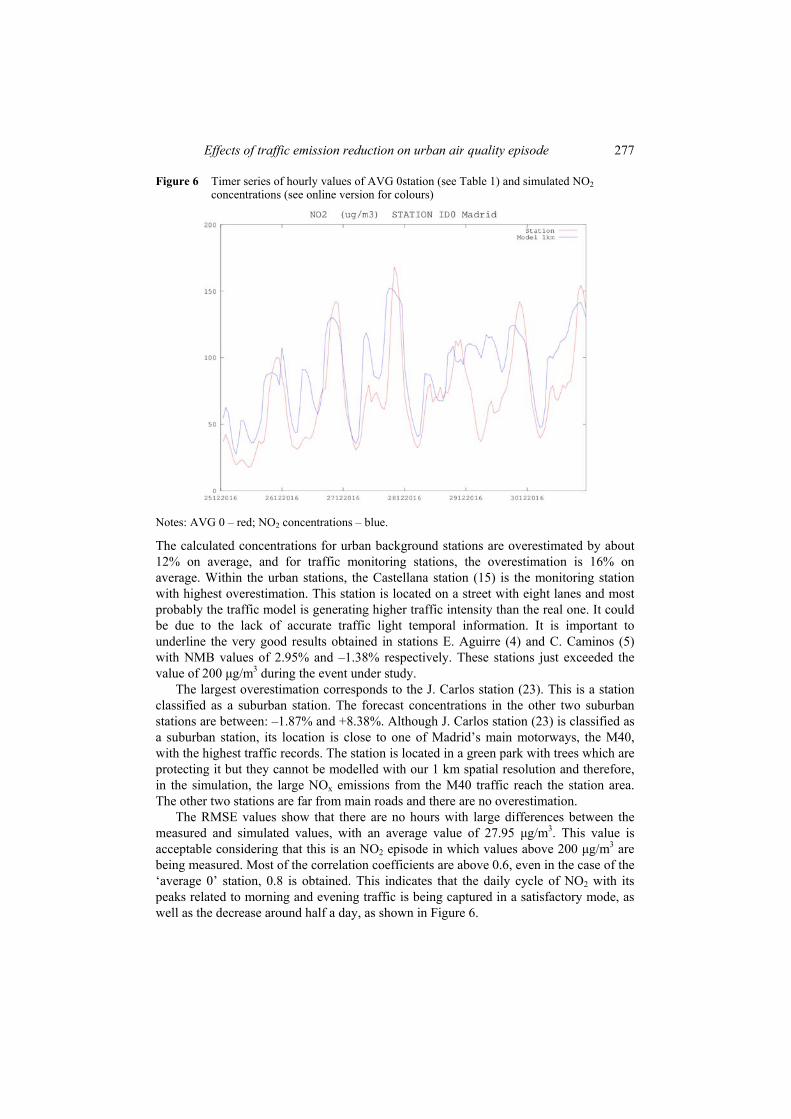
Figure 6 Timer series of hourly values of AVG 0station (see Table 1) and simulated NO2 concentrations (see online version for colours)

Notes: AVG 0 – red; NO2 concentrations – blue.

The calculated concentrations for urban background stations are overestimated by about 12% on average, and for traffic monitoring stations, the overestimation is 16% on average. Within the urban stations, the Castellana station (15) is the monitoring station with highest overestimation. This station is located on a street with eight lanes and most probably the traffic model is generating higher traffic intensity than the real one. It could be due to the lack of accurate traffic light temporal information. It is important to underline the very good results obtained in stations E. Aguirre (4) and C. Caminos (5) with NMB values of 2.95% and –1.38% respectively. These stations just exceeded the value of 200 μg/m3 during the event under study.

The largest overestimation corresponds to the J. Carlos station (23). This is a station classified as a suburban station. The forecast concentrations in the other two suburban stations are between: –1.87% and +8.38%. Although J. Carlos station (23) is classified as a suburban station, its location is close to one of Madrid’s main motorways, the M40, with the highest traffic records. The station is located in a green park with trees which are protecting it but they cannot be modelled with our 1 km spatial resolution and therefore, in the simulation, the large NOx emissions from the M40 traffic reach the station area. The other two stations are far from main roads and there are no overestimation.

The RMSE values show that there are no hours with large differences between the measured and simulated values, with an average value of 27.95 μg/m3. This value is acceptable considering that this is an NO2 episode in which values above 200 μg/m3 are being measured. Most of the correlation coefficients are above 0.6, even in the case of the ‘average 0’ station, 0.8 is obtained. This indicates that the daily cycle of NO2 with its peaks related to morning and evening traffic is being captured in a satisfactory mode, as well as the decrease around half a day, as shown in Figure 6.


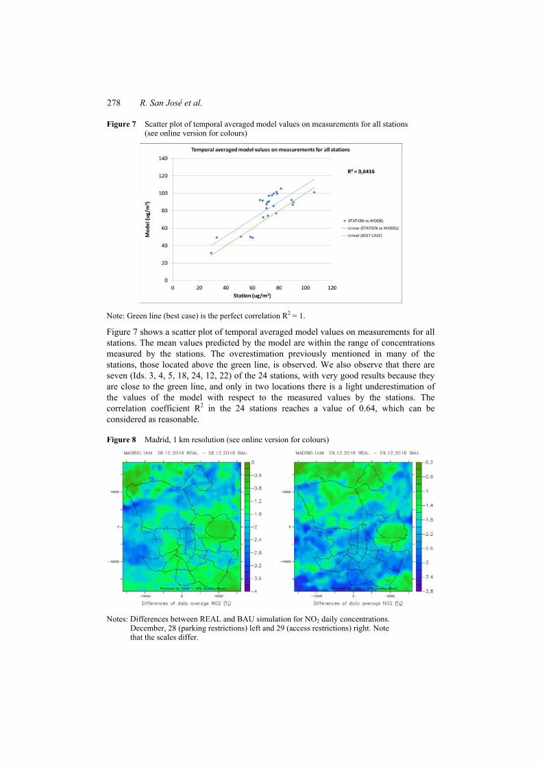
Figure 7 Scatter plot of temporal averaged model values on measurements for all stations (see online version for colours)

Note: Green line (best case) is the perfect correlation R2 = 1.

Figure 7 shows a scatter plot of temporal averaged model values on measurements for all stations. The mean values predicted by the model are within the range of concentrations measured by the stations. The overestimation previously mentioned in many of the stations, those located above the green line, is observed. We also observe that there are seven (Ids. 3, 4, 5, 18, 24, 12, 22) of the 24 stations, with very good results because they are close to the green line, and only in two locations there is a light underestimation of the values of the model with respect to the measured values by the stations. The correlation coefficient R2 in the 24 stations reaches a value of 0.64, which can be considered as reasonable.

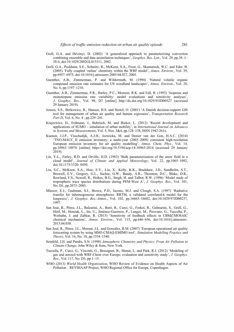
Figure 8 Madrid, 1 km resolution (see online version for colours)

Notes: Differences between REAL and BAU simulation for NO2 daily concentrations. December, 28 (parking restrictions) left and 29 (access restrictions) right. Note that the scales differ.


In a previous section, the modelling methodology was described and evaluated. Here, we present some results and discuss the impacts of the traffic restrictions on Madridair pollution. Figure 8 shows the spatial distributions of NO2 daily average relative differences (%) for REAL and BAU traffic conditions in the inner domain.

Figure 8 shows small differences between REAL and BAU NO2 concentrations (less than 4%, on average close to 2%) for days, 28 and 29 of December. The differences are more important on day 29than on day 28, so access restrictions have more impacts on NO2 concentrations than parking limitations. The reduction of the NO2 on day 29 reached more areas (blue areas) of the Madrid city than on day 28. The North of the city is the part where the traffic has less impact (green areas) on the air quality, so the lowest difference occurs in the North and small area in the East of the city for both days. In the South and centre of the city, reduction of NO2 concentrations by traffic restrictions occurs only on day 29.

Figure 9 Hourly variation of NO2 concentration at site E, Aguirre and for REAL and BAU simulation (see online version for colours)

Figure 9 shows time series of hourly surface NO2 concentrations modelled at E. Aguirre monitoring site for REAL and BAU simulations.

If we focus on the location where the highest NO2 concentrations were reached (E. Aguirre station), the traffic restrictions had soft effects, on day 28 –1.62%, on day 29 –2.04% and on day 30 –0.36%. Both simulations (REAL and BAU) are quite similar, so the traffic restrictions were not effective to avoid the NO2 episode.

5 Conclusions

An air quality modelling system has been implemented in the present exercise. The model includes an emission model (EMIMO), the SUMO traffic model and a pollutant transport and chemistry model (WRF/Chem). The complete modelling system has been applied to simulate an episode of high NO2 concentrations in the city of Madrid during December 2016 with high spatial resolution (1 km). The evaluation of the performance has been satisfactory, with good values in the correlation coefficients, although at some local points the system has not been able to reach the maximum (hourly average values)


peaks of NO2 concentrations measured by monitoring stations. Resolution of 1 km has not been enough to capture some very local concentration peaks. The modelling system correctly reproduces the day-night cycle and we believe that future system improvements should focus on simulating strong spatial NO2 gradients. Also, the a CFD model has to be used to simulate local effects with much higher spatial resolution using as boundary conditions the results produced in the present paper. This CFD model should use urban boundary layer effects to take into account the buildings and the complexity of urban environment to capture the complexity of local effects and reproduce the important local effects we have detected in the present work. We are working on integrating a CFD model (50 metres resolution) into the system to reproduce more accurately the observed air concentrations.

The SUMO traffic model results – as obtained in this experiment –, are fully applicable in the future CFD simulations (future work) because the SUMO model produces vector data which are adapted to any spatial gridded resolution. The modelling system has been used to evaluate the effectiveness of the traffic restriction scenarios (parking limitations on day 28 and day 30; access limitations on day 29) that were taken by the Madrid City Council to fight against the high NO2 concentrations. The evaluation was performed by comparing the REAL simulation (with traffic restrictions) with a BAU simulation (without traffic restrictions or business as usual scenario). Although traffic decreased by 10% on day 28, 16% on day 29 and 6% on day 30, NO2 daily concentrations decreased by only 1.5% on day 28, 2% on day 29 and 0.5% on day 30. These results show that the adopted scenarios were not effective enough when comparing with the effort to reduce the traffic. Other scenarios should be evaluated with less impact on citizens and with greater capacity to reduce the air pollution (transformation of diesel into electric vehicles, ban of driving to vehicles older than 15 years old, traffic speed reductions, focus only on the areas where higher impact is expected in the pollution concentrations using process and sensitive analysis in the model, etc.).

References Bergantino, A.S., Bierlaire, M., Catalano, M., Migliore, M. and Amoroso, S. (2013) ‘Taste

heterogeneity and latent preferences in the choice behaviour of freight transport operators’, Transp. Policy, Vol. 30, No. C, pp.77–91.

Binkowski, F.S. and Shankar, U. (1995) ‘The regional particulate matter model: 1. Model description and preliminary results’, J. Geophys. Res.-Atmos., Vol. 100, pp.26191–26209, doi:10.1029/95JD02093, 1995.

Chapman, E.G., Gustafson Jr., W.I., Easter, R.C., Barnard, J.C., Ghan, S.J., Pekour, M.S. and Fast, J.D. (2009) ‘Coupling aerosolcloud-radiative processes in the WRF-Chem model: investigating the radiative impact of elevated point sources’, Atmos. Chem. Phys., Vol. 9, pp.945–964, doi:10.5194/acp-9-945-2009, 2009.

Cohen, J., Cook, R., Bailey, C.R. and Carr, E. (2004) ‘Relationship between motor vehicle emissions of hazardous pollutants, roadway proximity, and ambient concentrations in Portland, Oregon’, Environmental Modelling & Software, doi: 10.1016/j.envsoft. 2004.04.002.

Easter, R.C., Ghan, S.J., Zhang, Y., Saylor, R.D., Chapman, E.G., Laulainen, N.S., Abdul-Razzak, H., Leung, L.R., Bian, X. and Zaveri, R.A. (2004) ‘MIRAGE: model description and evaluation of aerosols and trace gases’, J. Geophys. Res.-Atmos., Vol. 109, D20210, doi:10.1029/2004JD004571, 2004.

EEA (2013) European Environmental Agency (EEA) Air Quality in Europe – 2013 Report.


Grell, G.A. and Dévényi, D. (2002) ‘A generalized approach to parameterizing convection combining ensemble and data assimilation techniques’, Geophys. Res. Lett., Vol. 29, pp.38–1–38-4, doi:10.1029/2002GL015311, 2002.

Grell, G.A., Peckham, S.E., Schmitz, R., McKeen, S.A., Frost, G., Skamarock, W.C. and Eder, B. (2005) ‘Fully coupled ‘online’ chemistry within the WRF model’, Atmos. Environ., Vol. 39, pp.6957–6975, doi:10.1016/j.atmosenv.2005.04.027, 2005.

Guenther, A.B., Zimmerman, P. and Wildermuth, M. (1994) ‘Natural volatile organic compound emission rate estimates for US woodland landscapes’, Atmos. Environ., Vol. 28, No. 6, pp.1197–1210.

Guenther, A.B., Zimmerman, P.R., Harley, P.C., Monson, R.K. and Fall, R. (1993) ‘Isoprene and monoterpene emission rate variability: model evaluations and sensitivity analyses’, J. Geophys. Res., Vol. 98, D7 [online] http://dx.doi.org/10.1029/93JD00527 (accessed 29 January 2019).

Jensen, S.S., Berkowicz, R., Hansen, H.S. and Hertel, O. (2001) ‘A Danish decision-support GIS tool for management of urban air quality and human exposures’, Transportation Research Part D, Vol. 6, No. 4 , pp.229–241.

Krajzewicz, D., Erdmann, J., Behrisch, M. and Bieker, L. (2012) ‘Recent development and applications of SUMO – simulation of urban mobility’, in International Journal on Advances in Systems and Measurements, Vol. 5, Nos. 3&4, pp.128–138, ISSN 1942-261x.

Kuenen, J.J.P., Visschedijk, A.J.H., Jozwicka, M. and Denier van der Gon, H.A.C. (2014) ‘TNO-MACC_II emission inventory; a multi-year (2003–2009) consistent high-resolution European emission inventory for air quality modelling’, Atmos. Chem. Phys., Vol. 14, pp.10963–10976 [online] https://doi.org/10.5194/acp-14-10963-2014 (accessed 29 January 2019).

Lin, Y-L., Farley, R.D. and Orville, H.D. (1983) ‘Bulk parameterization of the snow field in a cloud model’, Journal of Climate and Applied Meteorology, Vol. 22, pp.1065–1092, doi:10.1175/1520- 0450.

Liu, S.C., McKeen, S.A., Hsie, E.Y., Lin, X., Kelly, K.K., Bradshaw, J.D., Sandholm, S.T., Browell, E.V., Gregory, G.L., Sachse, G.W., Bandy, A.R., Thornton, D.C., Blake, D.R., Rowland, F.S., Newell, R., Heikes, B.G., Singh, H. and Talbot, R.W. (1996) ‘Model study of tropospheric trace species distributions during PEM-West A’, J. Geophys. Res., Vol. 101, No. D1, pp.2073–2085.

Mlawer, E.J., Taubman, S.J., Brown, P.D., Iacono, M.J. and Clough, S.A. (1997) ‘Radiative transfer for inhomogeneous atmospheres: RRTM, a validated correlated-k model for the longwave’, J. Geophys. Res.-Atmos., Vol. 102, pp.16663–16682, doi:10.1029/97JD00237, 1997.

San Josè, R., Pèrez, J.L., Balzarini, A., Barò, R., Curci, G., Forkel, R., Galmarini, S., Grell, G., Hirtl, M., Honzak, L., Im, U., Jimènez-Guerrero, P., Langer, M., Pirovano, G., Tuccella, P., Werhahn, J. and Zabkar, R. (2015) ‘Sensitivity of feedback effects in CBMZ/MOSAIC chemical mechanism’, Atmos. Environ., Vol. 115, pp.646–656, doi:10.1016/j.atmosenv. 2015.04.030.

San José, R., Pérez, J.L., Morant, J.L. and González, R.M. (2007) ‘European operational air quality forecasting system by using MM5-CMAQ-EMIMO tool’, Simulation Modelling Practice and Theory, Vol. 16, No. 10, pp.1534–1540.

Seinfeld, J.H. and Pandis, S.N. (1998) Atmospheric Chemistry and Physics: From Air Pollution to Climate Change, John Wiley & Sons, New York.

Tuccella, P., Curci, G., Visconti, G., Bessagnet, B., Menut, L. and Park, R.J. (2012) ‘Modeling of gas and aerosol with WRF-Chem over Europe: evaluation and sensitivity study’, J. Geophys. Res., Vol. 117, No. D3, pp.1–15.

WHO (2013) World Health Organisation, WHO Review of Evidence on Health Aspects of Air Pollution – REVIHAAP Project, WHO Regional Office for Europe, Copenhagen.


Wild, O., Zhu, X. and Prather, M. (2000) ‘Fast-J: accurate simulation of in- and below-cloud photolysis in tropospheric chemical models’, J. Atmos. Chem., Vol. 37, pp.245–282, doi:10.1023/A:1006415919030.

Zaveri, R.A. and Peters, L.K. (1999) ‘A new lumped structure photochemical mechanism for largescale applications’, J. Geophys. Res., Vol. 104, No. D23, pp.30387–30415.

Zaveri, R.A., Easter, R.C., Fast, J.D. and Peters, L.K. (2008) ‘Model for simulating aerosol interactions and chemistry (MOSAIC)’, J. Geophys. Res., Vol. 113, D13204, doi:10.1029/ 2007JD008782.

Zhang, Y., Bocquet, M., Mallet, V., Seigneur, C. and Baklanov, A. (2012) ‘Real-time air quality forecasting, part I: history, techniques, and current status’, Atmos. Environ., Vol. 60, No. 1, pp.632–655.

effects of traffic emission reduction on urban air quality

Documents