[ . 9 EiEI}'- FAD

REPORT NO. 1311

THE METHOD OF LINES FOR NUMER ICAL SOLUTION OF

PAR TI AL D I FFER ENTI AL EQUATI ONS

by

Tadeusz LeserJohn T. Harrison

March 1966

CL E AR I NG H OD&J Luloz of this doc'~ment isunimimted.FOR DERAL SCIRNTIFIC AND

TECH iNICAL INFORMATION

'••°( 'f~~r~ttch°'•l ... '" • ppI'

U. S. ARMY MATERIEL COMMAND UG 17 1966BALLISTIC RESEARCH LABORATORIESABERDEEN PROVING GROUND, MARYLAND . L 6j

C

Destroy this report when it in no longer needed.Do not return it to the originator.

The findings in this report are not to be construed asan official Department of the Army position, unlessso designated by other authorized documents.

16

BALLISTIC RESEAiRCH LABORATORIES

REPORT NO. 1311 ZCESTIO -foI

CFSTI W;1ITE S!CIONPACD OC O UiF SECTION lJ

MALRCH 1966 AUNE

DISTi BU8ION/AVAILABILITY CODES

MIT•1. •AVAIL. and cr S,,GCIAL

Distribution of this document is unlimited.

THE METHOD OF LINES FOR NUMERICAL SOLUTION OFPARTIAL DIFFERTIAL EQUATIONS

Tadeusz LeserJohn T. Harrison

Computing Laboratory

RDITE Project No. 1PO14501A14B

ABERD)EEN PROVING GROUND, MARYLAND

BALLISTIC RESEARCH LABORATORIES

REPORT NO. 1311

TLeeser/JTHarrison/blwAberdeen Proving Ground, Md.March 1966

THE METHOD OF LINES FOR NUMRICAL SOLUTION OFPARTIAL DIFFERENTIAL EQUATIONS

ABSTRACT

In the method of lines for solving certain kinds of boundary value

problems in rectangular or trapezoidal regions one of the variables, say

y, is discretized while the other variable x is left continuous. When

suitable finite difference approximations are substituted for the partial

derivatives with respect to y the differential equation is changed into

a simultaneous system of ordinary differential equations in the variable

x. The method used very little in the USA is used e)oniiveLy in the

Soviet Union and nearly all the literature on this subject is in Russian.

The method has been tried in BRL and it seems to be a very useful one.

This report does not pretend to be a monograph on the subject. It

intends to be a practical guide to computations.

TABLE OF CONTENTS

Page

ABSTRACT. a . . . a . . . . a . . . . . . . a a * a . . * . a . 3

THE PRICPLE G••M T ETHOD OFLINES.. ..... . . . ... 7

THE LAPLACE EQUATION.... .. .. . . . . . . . . o 9A HIGCR ORDER OF APPROXIMATION FOR THE LAPLACE (OR POISSON)EQUATION. o . . . . . . . . . . . . . . . . . . . . . . . o . 0 9

THE CLOSED SOLUTION . . . . . . . ... s * 0 a * 0 * 9 0 0 0 * * 0 10

NI24ERICAL EXAMPLE 1 o .0. . . . . . . . . f ..0. . . . . . . .e. 14

THE PARTICULAR INTEGRALS . . . . . . . . . o .o . . . . o . . 15

THE GENERAL SOLUTIONS . o o . . ..o. . . .o o . . . . . . . . . 15

NU1MERICAL EXAMPLE 2 . . . .*. . . . . . . .. .. . . . . . . . . 16

EXcAMPLE 3 o . o * .0. . . . . . . . . . . .0 . . . . . . . . . 20

MACHINE COMPUTATION s * 9. .. . . . . . . . . . . . . . . . . . 22

CONCLUSIONS .. . . .o . .o s .o • o . . • • . . . * .0 .0 . . . 22

REFERENCES. .. . . . • s o . s . . . . . . . . • . . .a. . . . 30

DISTRIBUTION LIST . a o a • • .o. . .& * o o • o o o o • • • 31

ME PRINCIPLE OF THE NETHOD OF LInEf

We shall explain the method of lines for the following differential

equation of the second order in two variables which is to be integrated

in the rectangular region.

R; a xS ; y o y yo +L

with boundary C.

Our boundary value problem is

au + bu +cu + du + eu +fu a gxy yy x ynR 1

u(x, yo) - q(x); u(x, yo + L) . ql(x) (2)onC

u(a, y) = p0(y); u(P, y) - pl(y) (3)

where a, b, c, d, e, f, g are functions of x and y, and qi and p are

prescribed functions of x and y and all of these functions are continuous.

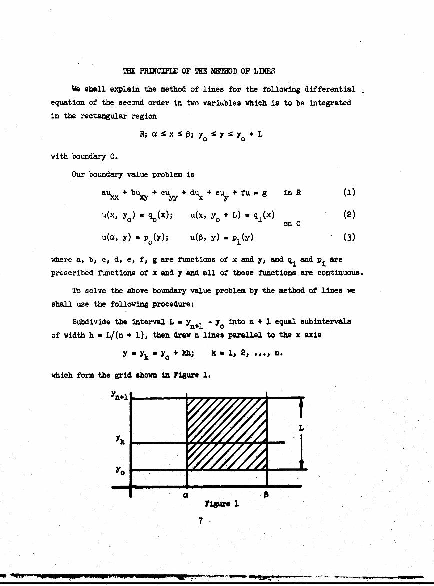
To solve the above boundary value problem by the method of lines we

shall use the following procedure:

Subdivide the interval L - Yn+l - Y. into n + 1 equal subintervals

of width h a L/(n + i), then draw n lines parallel to the x axis

y = Yk a yo + kh; k , 1, 2, *,., n.

which form the grid shown in Figure 1.

Yn+l

Yo

a 1

7

We asstume that both the first and the second order partial derivatives

are continuous in x and y. Then we substitute in Equation (1)Y" Myk; (k- 1, 2, .,.., n)

and replace the partial derivatives with respect to y by the central

differences

Uy(X, yk)- (2h)"i [Ukl(x) - Uk-l(X)]

uyy(x, Yk)" (h)2 [Uk+l(x) - 2Uk(x) + Uk-l(x)]

U, (x, k) (2h) 1 [Ui.(x) - qk.l(x)1

where

uk(x) ,U(x, Yk); U(x) = (d/dx)(U(xyk)), and Uk(x) is an

approximation of u(x, yk) on the line y w Yk"

When we perform these substitutions we obtain a system of n simul-

taneous differential equations of the second order which approximates

the system Equations l) and (2):

au, + (2h))bk(Ui1 - _.,) + h'ck(Ul - 2Uk k Uki) + dU• (d)

+ (2h) ek(Ukl - Uk-1) + fkuk a ; k a 1, 2, .,., n.

The boundary conditions become

Uo(x) . (x); Un1 (x) -= (x) (•)

uk(a) a ro(yk); Uk(A) a P(k). (6)

Nov Equations (5) are no longer considered to be boundary conditions.

They determine certain terms in the equation for k a 1 and for k a nbelonging to system (4). Ohe Equations (6) are the 2n boundary conditionsfor the n second order differential Squations ().

8

The simultaneous system of ordinary differential Equations (4) and

(5) together with the 2n boundary conditions equation (6) approximate the

boundary value problem Equations (I), (2), and (3). The general solution

of Equations (4) and (5) depends linearly on the 2n arbitrary constants

of integration which are determined from the 2n boundary conditions

Equation (6).

The convergence of the approximating system Equations (4), (5), (6)

to the original system Equations (1), (2) and (3) when h approaches zero

under certain restrictions on the coefficients and on the boundary1*

conditons has been proven by various Soviet mathematicians

THE LAPLACE EQUATION

Consider the boundary value problem Equations (i), (2) and (3) when

the left member of Equation (1) is the Laplacian

U u +u - g(x) . (lA)xx yy

In this case the approximating system of Equation (4) takes the form

U'f + h 2(Uk+1 - 2Uk + Uk.1) a gk; k l, 2, ., n. (4A)

The Equations (5A) and (6A) would be the same as Equations (5) and (6).

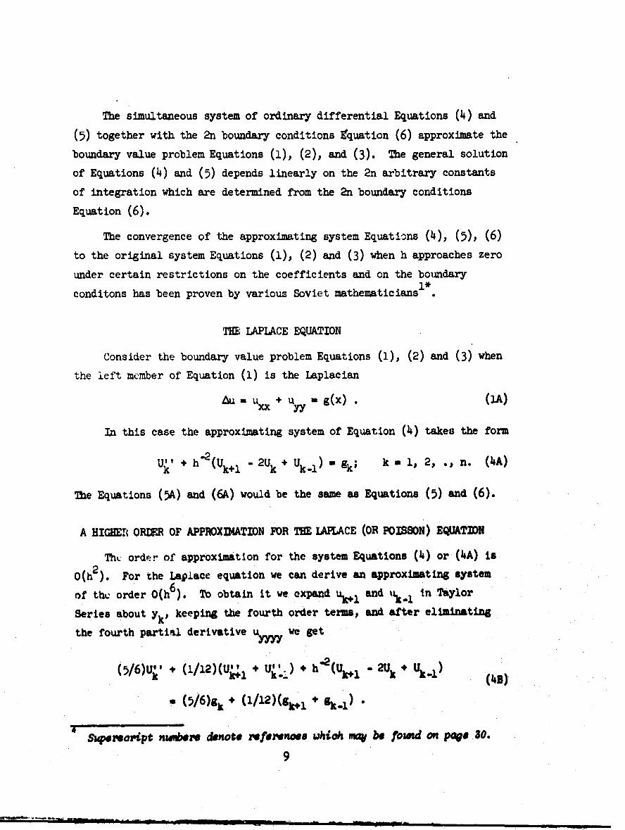
A HIGHER OREER OF APPROXDIATION FOR THE LAPLACE (OR POISSON) EQUATION

Thc order of approximation for the system Equations (4) or (4A) is

O(h2). For the Laplace equation we can derive an approximating system

of the order O(h 6). To obtain it we expand uk•1 and ik., in Taylor

Series about Yk' keeping the fourth order terms, and after eliminating

the fourth partial derivative u we get

(5/)Uj + (1/12)(U;;, + ujI..) + h -2 (Uk1 -2Uk + Uk.1)O(B)

(5/6)gk + (1/12)(gk, 1 + 9k.1)

iAperseript nw~eve denote refewnioe uhioh mV be found opt ptV* SO.

ME CLOSED SOLUTION

For the Laplace equation and when the prescribed values of u on the

lines y = yo and y - yn- 1 are zero, we can obtain a simple closed solution

for each line.

Consider the boundary value problem Equations (1), (2), and (3),

when q . O, which is approximated by

U11 + h-(Ukl - 2 Uk +Uk.l) - 0; k - 1, 2, .,, (4A)

Uo(x).= Un.l¢•) - o, (A)

U(a, yk) - po(yk); U(, yk) - pl(y.); k = 1, 2, .,., n. (6A)

Applying the separation of variables we assume the following form

Uk(x) - q(k)v(x)

and substitute it into the above homogeneous equation. Ibis yields the

following equation:

q(k)v"(x) + h-2v(x)[q(k + 1) - 2q(k) + q(k - . 0

q(O) a q(n + 1) - 0

or

V"(x)/v(x) a + 1) - 2q(k) + q(k - - h2q(k) a 52 constant.

To find q we must solve the homogeneous difference equation

q(k -1) - [2 -h282]q(k) + q(k - 1) *0

vith the boundary conditions

q(0) - q(n + 1) 0-.

lbe general solution of this difference equation has the form

k kq(k)m C1?1 +' C2X2

10

where C1 and C are arbitrary constants and X and X are the roots of1 2 1 2

the characteristic equation

x2, [2-h28]%+ 1- 0.

From the boundary conditions we have

q(O) - C1 + C2 - O, hence C2 - - C1

q(k + 1) - C( 1 Xi1 - x2 ) - O, hence (X1/X2)nl+ -1

and

(x,/X2) exp (2ff is/(n + 1))

From the characteristic equation we have that

?IX - 11 x2

consequently

. "exp(W is/(n + l)) ;

'2" exp( - W is/(n + M))

. (y - yo)/h *, ,2 .. n

From the characteristic equation we have also that

Xz X 2 h 2 5 h281h 2

consequently

S•022 exp(, ±s/(n + 1)) + exp(- I is/(n + 1))= 2 coe(is/(n + 1))

2 2.2 2 -aos(m/(,{ + 1)) - $i. -(-(y -yo)/2L

q.(k) - c[Cxp(,ft isk/(, •)) - exp(- it isk/(n. +))] C Sit(,. - yo)/L).

11

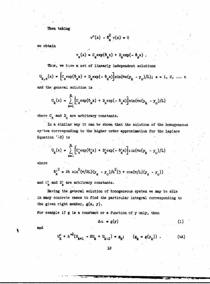
Then taking

v"(x) - 82 V(X) 0 0

we obtain

vs(x) - Csexp(8 sz) + Dsexp(- 8sX)

Thus, we have a set of linearly independent solutions

Uk.,S(x) - ICSexp(b sx) + D 8exp(- 5 sx)] sin(1Ts(yk -yo)/L); s = 1 2, ... n.

and the general solution is

Uk(x) [C s [exp(B Sx) + D sexp(_- B a x)lsin (Trs (Yk.- yo)/L)S=I.

where C5 and D are arbitrary constants.

In a similar way it can be shown that the solution of the homogeneous

syrtem corresponding to the higher order approximation for the Laplace

Equation '1B) isn

Uk(X) = Z [Csexp(bsx) + Dsexp(- sX)]•zn(ns(Yk - Yo)/L)s-l

where

5s2 24 sin2 (T/2L)(ys - yo)/h 2(5 + cos(Tr/L)(y. - yO))

and C' and D' are arbitrary constants.

S s

Raving the general solution of homogeneous system we may be able

in many concrete cases to find the particular integral corresponding to

the given right member, g(x, y).

For example if g is a constant or a function of y only, then

Au - g(y) (1)

and(f"+* h'(uk~i " Uk ÷U U -1 g- g g( . (4A)

12

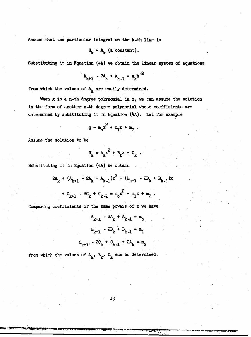
Assume that the particular integral on the k-th line is

Uk a Ak (a constant).

Substituting it in Equation (4A) we obtain the linear system of equations

A k+l -2+A A - h -2

from which the values of Ak are easily determined.

When g is a n-th degree polynomial in x, we can assume the solution

in the form of another n-th degree polynomial whose coefficients are

d,ttermined by substituting it in Equation (4A). Let for example

2gmo0 X + mx+m 2 •

Assume the solution to be

Uk •A 2+ kx+ Ck

Substituting it in Equation (4A) we obtain

22A k+ (A +l ~2A k +A k-l)x 2+ (B k+l -2B k+,B kl)x

k+- 2 Ck Ck. =mx + mlx + m2

Comparing coefficients of the same powers-of x we have

A k+l -2A k + Ak -i m 0

Bk+l-2Bk + Bk, m

Ck~l : 2 Ck + Cki + 2Ak =-m2

from which the values of Ak, B k Ck can be determined.

13

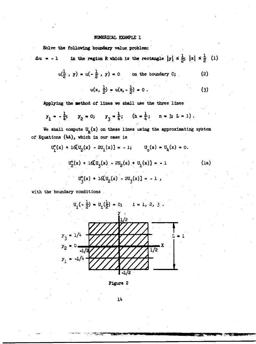
NU!EUCAL EXAMPLE 1

Solve the following bowndary value, problem:• .-- 1 1ntheregion •,whichis the rectangley l - ICI (€)

u )l 1 yA- 0 on the boundary C; (2)

u(x, U) u(x,- ).o. (3)

Applying the method of lines we shall-use the three lines1 11. 3L=)

y 2 o; Y3 = T; (h v; = 3; L -)

We shall compute Uk(x) on these lines using the approximating syistem

of Equations (4A), which in our case is

Tf'(x) + 16•U 2 (x) - 2U(x)] = - 1; Uo(x) U4 (x) = 0.

Uf(x) + 6Cu 3 (x)- 2U2 (x)+ U1(x)] . - j (1a)

UIf(x) + 16[U2 (x) -2u3(x)] = - ,

with the boundary conditions

ui(- L)" U (1) 0 0; i = 1, 2, 3

3y1/2

Y2

-1/ 1

Figure 2

14

n1E PARTICULAR INTEGRALS

We shall assume that the particular integrals of our system are

the constants

Ui=Ai,

Substituting the above in the system Equation (la) we obtain

A, A 3 3/32; A2 1/8

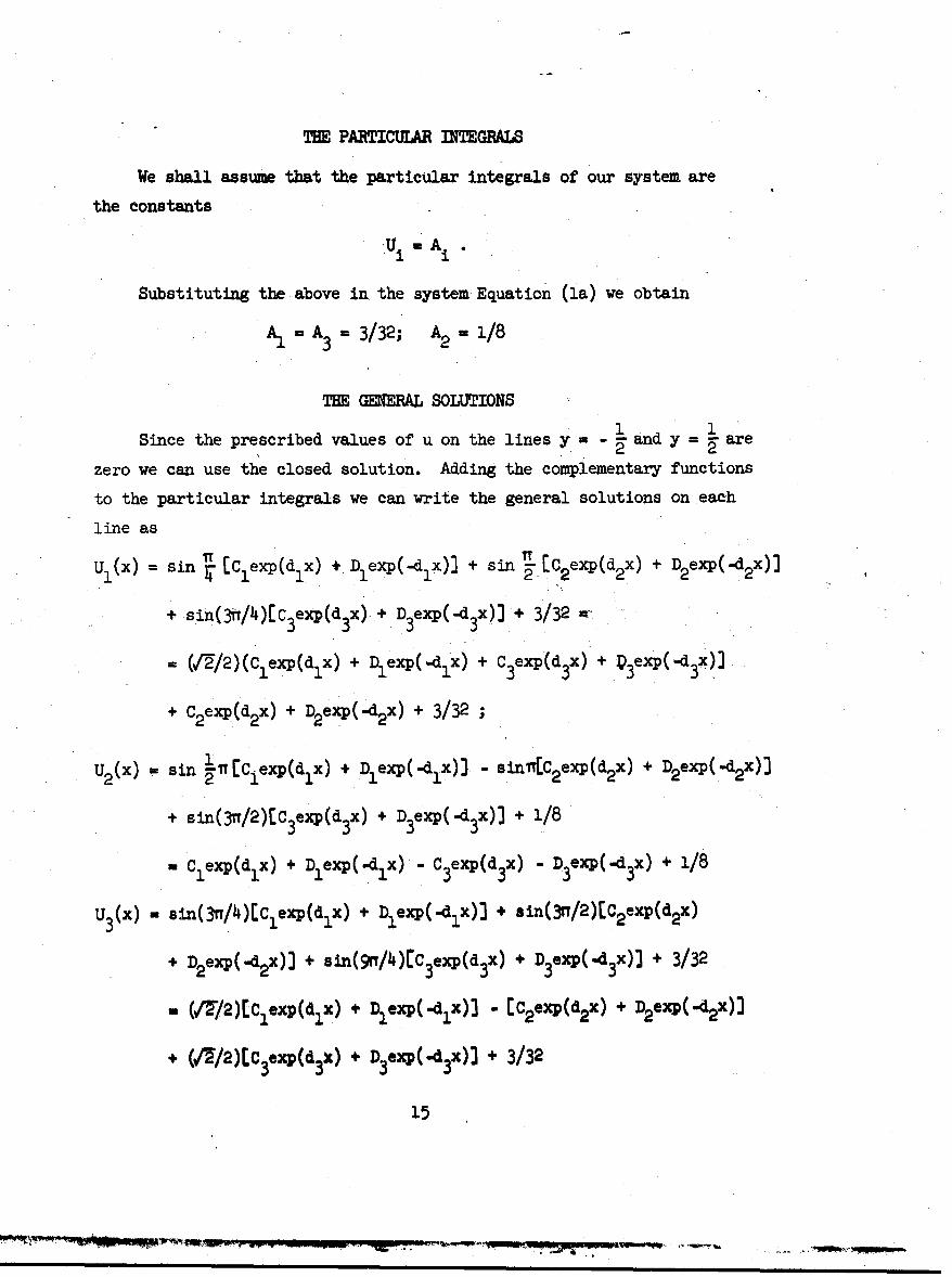
THE GENERAL SOLUTIONS1 1

Since the prescribed values of u on the lines y = - and y = 2are

zero we can use the closed solution. Adding the complementary functions

to the particular integrals we can write the general solutions on each

line as

Ul (x) sin • [Clexp(dlx) + Dlexp(-dlx)] + sin '_[C 2 exp(d 2x) + D2exp(-d 2x)

+ sin(3fr/4)[c 3exp(d 3x)- + D3exp(-d 3x)] + 3/32

(/F/2)(C exp(dix) + Dlexp(-dlx) + C exp(d 3X) + p3exp(-d 3 4c))

+ C2 exp(d 2 x) + D2 exp(-d 2 x) + 3/32 ;

U2 (x) - sin 1Tr[C1 exp(d 1x) + D1exp(-dlx)] - sinTnC 2 exp(d 2 x) + D2 exp(-d 2 x)]

+ sin(3ff/2)[eC3exp(d 3x) + D3e xp(-d 3 x)4 + 1/8

-C1 exp(d1x) + D1 eexp(.dlx) - C3 exp(d 3 x) - D3 exp(-d 3x) + 1/8

U3 (x) - sin(3rT/4)EC 1exp(djx) + Dlexp(-d 1x)3 + sin(3fr/2)IC2 exp(d 2x)

+ D2 exp(-d 2x)] + sin(9rr/4)[C3exp(d 3x) + D3exp(.d 3x)l + 3/32

- (f7/2)[C 1exp(d1x) + Dexp(mdlx)) - [C2exp(d2x) + D2exp(-d 2x)]

+ (1'/2)[.C3exp(dB3 X) + D3exp(-d 3x)] + 3/32

15

'T

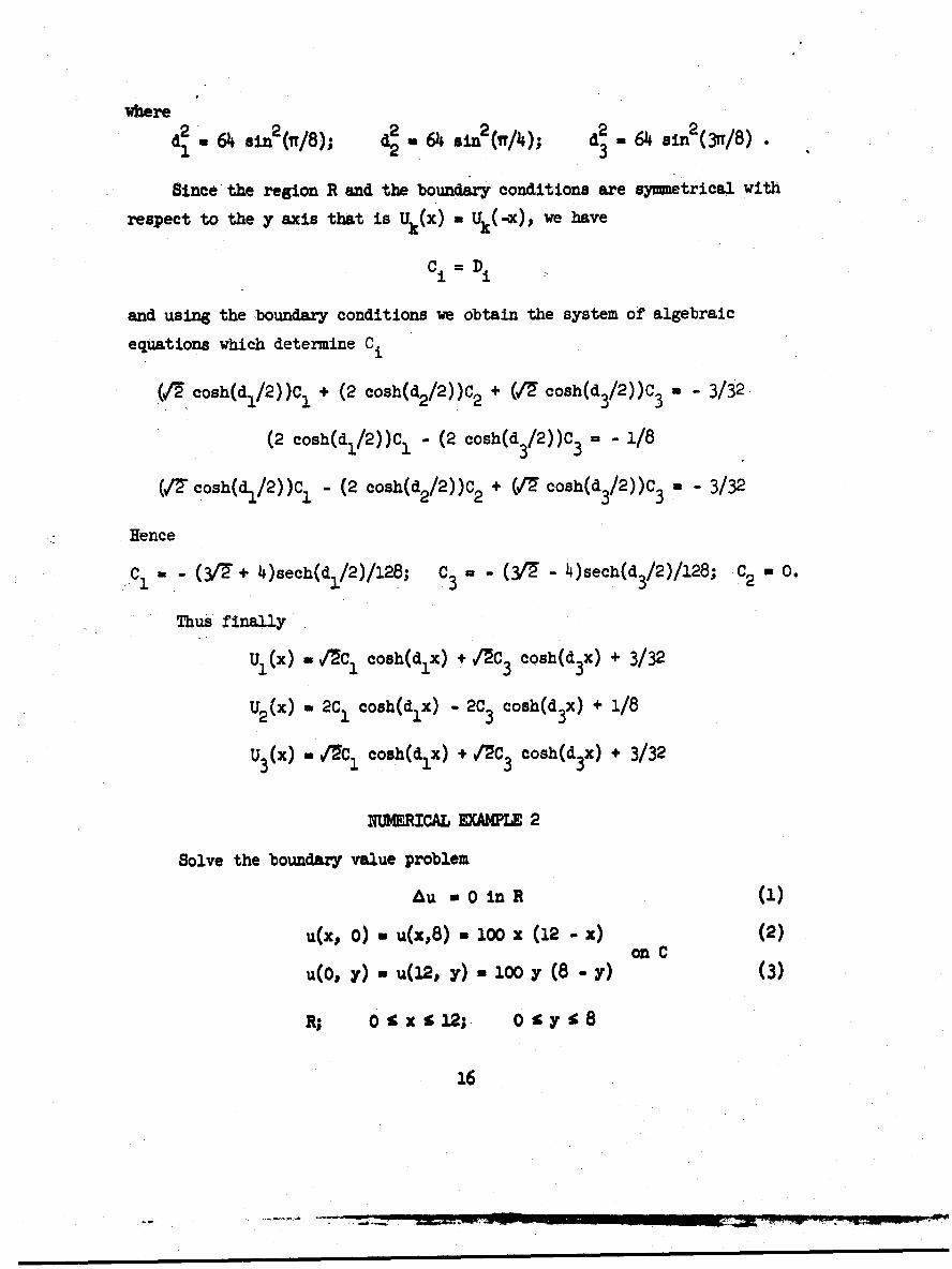
where2 2 2 2 2 2,

d 64sn*T/) 64 sin (-R/4.); d3 64 sin(3n,/8)

Sinceethe region R and the boundary conditions are sytmetrical with

respect to the y axis that is Uk(x) Uk(-x), we have

C1 =D,

and using the boundary conditions we obtain the system of algebraic

equations which determine Ci

(/Y cosh(dl/2))C1 + (2 cosh(d 2/2))C 2 + (/ý cosh(d 3/2))C 3 - - 3/32

(2 cosh(d 1/2))CI - (2 cosh(d 3/2))C -3 1/8

(VT ',osh(dl/2))C 1 - (2 cosh(d 2/2))C 2 + (/7 cosh(d 3/2))C 3 - 3/32

Hence

C1 = - ( +'2 4)sech(dl/2)/128; C3 = - - 4)sech(d3/2)/128; C2 - 0.

Thus finally

Ul (x) a /vC 1 cosh(dlx) + /2C3 cosh(d 3x) + 3/32

U2(x) = 2C1 cosh(dlx) - 2C3 cosh(d 3 x) + 1/8

U3 (x) - /TC1 cosh(dlx) + /2C3 cosh(d 3x) + 3/32

NUNERICAL EXAMPLE 2

Solve the boundary value problem

Au oin0 (1)

u(x, 0) a u(xs8) a 100 x (12 - x) (2)on C

u(O, y) = u(12$, y) OO y (8 - y) (3)

R; 0 A x 12;, Oiy 8

16

y

y2=--I - 2-

S, X

Figure 3

Applying the method of lines we shall use the three lines

Yl= 2, y2 = 4, y3 = 6; (h = 2, n u 3, L - 8).

We shall compute Uk(x) on these lines using the approximating

system Equation (4B) which in our case is

(5/6)uj + (1/12)(uf1 + uj.1) + h'2(Uk+l - 2Uk + Uk.1) . 0 (4B)

U0(x) U4(x) - 100 x (12 - x) (5B)

Uk(o) - Uk(12). 100 yk(8 - yk); k a 1, 2, 3. (6B)

We shall rewrite the system combining Equations (4B) and (5B)

(5/6)' + (1/12)(u - 200) + (1/4)(U2 - 2U + loo x (12•- x)) . o(5/6) , + (1/12)( , u+') i (1/4)(u3 -2U2 + 5) o (4B)

(5/6)U't + (1/12)(-200 + Ui#) + (1/4)(1oo x (12 - x) - 2U3 + U2 ) "0

a 2; 13(0) a 1920; U1(12) a 1200

Y . 4; U2(0) 1600; (12) 1600 (6B)

•3 -6; U3(0) 2oo; U3(12) - 12oo.

17

For digital computations the second order system must be reduced to

an initial value first order system. To achieve this let us set

U' .V (I)

2 l V 2 , (II)

Ut V3 ; (iii)

Substituting Equation (I), (II), .(III) in Equation (4B) we obtain

(5/6)v{ + (ll/2)(VL - 200) + (l/4)(u2 - 2U, + 100 x (12. x)) l 0 (Iv)

(516)vL + (¢ll2)(vi + vj) + (l/4)(u3 - 2U2 + U1) 0 Mv)

(5/6)Vj + (1/12)(-200 + VL) + (l/4)(lO0 x (12 - x) - 2U3 + U2 ) 0o (VI)

or

Vj + (1/1/o)v2 + (3/1o)U 2 - (6/10)11 a 20 - 30 x (12 - x) (Iv)

V+ + (l/lo)(vi + V{) + (3/1o)(u 3 - 2U2 + U1) 0 (v)

vi + (1/lo)v• - (6/10)u3 + (3/1031J 2 - 20 - 30 x (12 - x) (VM)

The Equations (I) through (VI) form the system of six first order

equations, two of them nonhomogeneous. The conditions Equation (6B),

however, are not all initial and we have to arrange for that. The

solution on any line k will be the linear combination of independent

solutions of the homogeneous sytem q plus the particular integral Ul

Uk(X) * c,€q(x) . UP(x) k . 1, 2, 3, (vII)

where C are constants to be determined from the boundary conditions.

The independent solutions of the homogeneous system Equations (I)

through (VI), where the right members in the Equations (IV) and (VI) are

replaced by zeros, are obtained frcs the folloving set of initial condi-

tions at x :O18

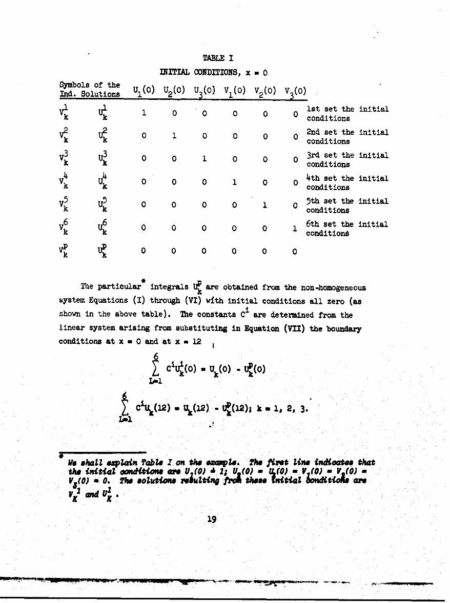
TABLE I

INITIAL CONDITIONS, x = 0

Slymbols of themnd. Solutions UI(O) U2 (O) U3(0) VI(o) V2 (O) V (O)

V 1i000 0 st set the initialki 0 0 0 0 0 conditions

V2k e 2nd set the initial0 1 0 0 0 0 cniink k conditions

V3 U3 3rd set the initial0k k conditions

44 4th set the initialVk Uk 0 0 0 0 conditions

V5 U5 0 0 0 0 1 0 5th set the initialk k conditions

V6 6 6th set the initial0ki conditiont

VP T? 0 0 0 0 0 0k k

"*The particular integrals Up are obtained from the non-homogeneous

ksystem Equations (I) through (VI) with initial conditions all zero (as

shown in the above table). The constants Ci are determined from thelinear system arising from substituting in Equation (VII) the boundary

conditions at x 0 and at x n 12

6SCoU(o) U (o)- t(o)

L-1

CiUk (12) -U(12) * J(12); k lp1 2P,3

ho We ehaZ ein Tabte Z1 on mhe eiirZ. The fiet; tine at"0eehth init eanditio awe U,(O) A1.' V (0) - r,(0) -a V(0) - VI(o) -

V (0) a . TVe ot utio.w •r nf fa tes nitat £ tioL a'V1 and U1

19

cuRviLzEAR BOUNPARIES

If the region of integration R is of a shape of a curvilinear

trapezoid shown in Figure 2 which is bounded by the lines

y a yo; and y -Yn+i

and by the curves

xac9(y) and x 0(y); yo0 y!Yni

then the procedure of the method of lines remains essentially the same

as for a rectangular region. The proof of convergence, however, requires

that the third partial derivative with respect to y be continuous. The

curvilinear boundaries will be explained in the following example.

EXAMPLE 3

Solve the boundary value problem

Au- 0 in R (1)

u(x0 o) = u(x, 4) a o (2)

on the curve a u ayl(x, y) n x + y (3)

on the curve f u a y2(x, y) a x -y

where R is c(y) % x . 0(y); 0% y 4

y 4 - 'Yk

a1 2

y1 - I....----yo = 1 2 3 5 6 7 8

2O

A w

3m • • • ••• • • . i

Applying the method of lines we shall use the three lines

yl - 1; Y2 = 2; y 3 " 3(h =- , n 3, L- 4)

We shall compute Uk(x) on these lines using the approximating

system of Equations (4A) which in our case is

U"U• U - 2U +U 0 0; U = oa0;

3 2

On the curve a; 1 2

Uk1 (ce)x +yk= yk Yk +y l

On the curve 0; Uk(0L) e- y -y e3k

where xkl is the abscissa of the point of intersection of the l1ne y Yk

and the curve x - az(y), and xk is the abscissa of the poinr of inter-

section of the line Yk and the curve x - 0(y).

Like in the previous examples we obtain six independent solutions

from the assumed initial values shown in Table I and form the general

solutionc6

U (x) UZc'u'(x)

Lai1

We determine the constants C from the linear system &rising from

•ulstltutine th.ý boundary conditions

UkX). C' i(X•); k 1p 2P 3.

21

MACHNE= COMPUTATION

In order to compare the method of lines with the conventional grid

method, Numerical Example 2 has been programmed using the two methods.

The programumling, with notation included, for the method of lines is

given. Figure 5 is a flow chart showing computer operations.

CONCLUSIONS

The method of lines and the conventional grid methods have been

compared on two high-speed digital computers at Ballistic Research

Laboratories, Computing Laboratory, Aberdeen Proving Ground, Maryland,

with respect to run time, computer limitations, and one known solution,

u(4, 4) = 2428. Let "H" be the step size and "N" be the number of points.

The comparisons follow:

First Method - Conventional Grid Method

A. H 2 N 15 15 x 15 Matrix

ORDVAC - Run Time 5 min.No Limitations

BRLESC -R Time 1 min.No Limitations

U(4, 4) - 2419.53919

B. Hl N 77 T7 x 77 Matrix

ORDVAC -Memory too small

BR1ESC -Run Time 1 minNo Limitations

u(4, 4) a 2420.694W

C. H .5 N a308 308 X30 Matri.x

Memory too small on both computers

22

* *;'. - -- - = -

lo LN 0

I9Jt

Al

.0

9' Io Joe

.hi~a~23

M- ' -

Sec.ond Method - Method of Lines

A. H 2 N 3 X = .1 6 x 6 Matrix

ORINAC - Run Time 5 min.Limitations, smaller LaX' s consume too much

run time

BRJESC - Run Time 1 min.No Limitations

u(4, 4) 2420.4529

B. H =1 N =7 AX = . 14 x 14 Matrix

ORDVAC - Run Time 10 min.Limitations, same as A.

BRLESC - Run Time 1 min.No Limitations

u(4, 4) 2420.7435

The method of lines needs approximately ten times less storage than

Lhe conventional finite difference methods. In some cases it may be

faster and more accurate. Another advantage of this method is its

applicability to analog computers.

TA'USZ LESER JOHN T. BARRISON

24

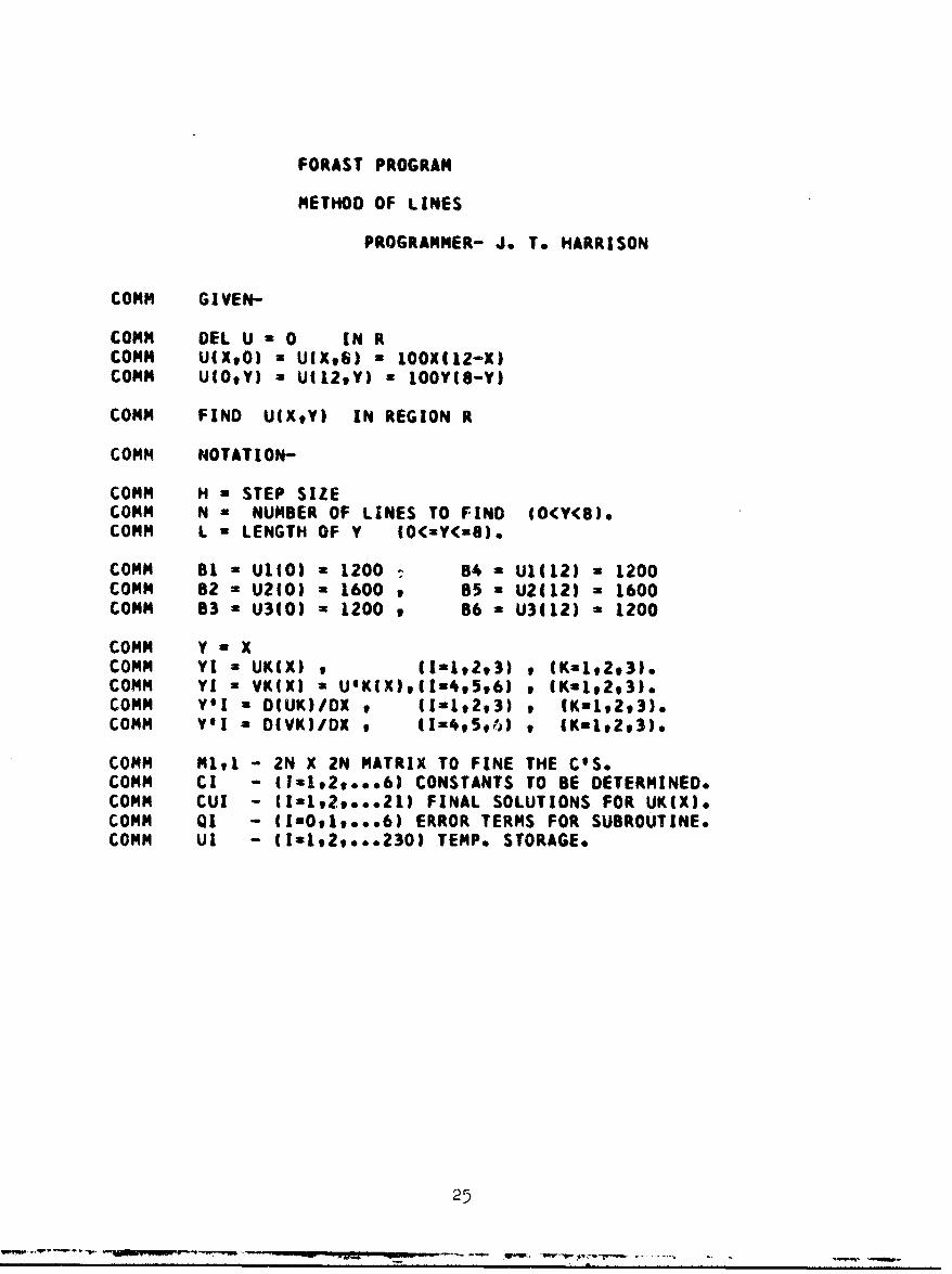
FORAST PROGRAM

METHOD OF LINES

PROGRAMMER- J. T. HARRISON

COMM GIVEN-

COMM DEL U 0 IN RCOMM U(XO) = UIX,6) = iOOXI12-X)COMM U(OY) - UiI29Y) 8 lOOY(8-Y)

COMM FIND U(XtY) IN REGION R

COMm NOTATION-

COMM H = STEP SIZECOMM N 8 NUMBER OF LINES TO FIND (O<Y<8).COMM L a LENGTH OF Y WO(-Y<-8).

COMM BI a UI1O) a 1200 0 84 a U1(12) a 1200COMM 82 z U2O0 a 1600 9 85 a U2(12) a 1600COMM B3 a U340) a 1200 9 B6 a U3412) a 1200

COMM y a XCOMM Yl a UKIX) , (1=19293) 9 (K01,293).COMm YI a VK(X) a UIKiX),(I=4,5,6) , (K=192,3).COMM YlI = D(UK)/OX , (1=012,3) , (K=B12,3).COMM Y'I = D(VK)/DX 9 (1=495,•41 IK9l,293).

COMM M1,1 - 2N X 2N MATRIX TO FINE THE COS.COMM CI - (l-lt2t...6) CONSTANTS TO BE DETERMINED.COMM CUI - (Is1l2,...21) FINAL SOLUTIONS FOR UKIX).COMm QI - (1=0,1,...6) ERROR TERMS FOR SUBROUTINE.COMM UI - (i=t2t..230) TEMP. STORAGE.

25

BLOC(Y-Y6) Iy'-Y'6)1Q0-06) ISI-S6)2BLOC(Ul-U230)1CUl-CU4S)(MLtl-M6,7)XBLOC1CI-C6)ZSYN (KaYIS

DELI DEC (.111START INTIH=Z21 INT1Nm3) INT1L=S)t

PRINT-FORMATIF3)-< H a >(H)< N a>(N)CONT< L a >(1)2

ENTER(PRINTS)l ENTER(PRINTB)l

Comm BOUNDARY CONDITIONS

81=12002 B2=160OX 83=1200284=12002 85=16002 86m1200l

Comm INTERGRATE (0<=X<=12)v BY MEANS OFComm A SUBROUTINE. RUNGE-KUTTA GILL TO APPROXIMATEComm ORDINARY DIFF. EQS. FROM ? INITIAL CONDITIONS

EPS=DEIX*.Sg5SET(TC=0)(1.0)2

1.0 READ-FORMATI Fl)-(?)NOS.AT(YO)2 INC(TC=TC*1 32SET(C=O)XUII.Y1X U29IaY2% U39l=Y3XINCI 1=1#3)XENTER(ReK.G.)(DELX)(?)1EYAL'YIY) YIYI) Q32COUNT120 IINIC)GOTO(R*K.G1)2 G0T014*0)X

Comm EVALUATE THE YIS.

EVALBY Y01sY42 Y12*Y5% Y*3nY6XIF-INT1TC=?IGOTO12.0)3HON = 0X GOTO( 3.0)2

2.0 HON a 20-30*XI12-X)23.0 AA=*6*Y1-o3oY2*HONS BBa-*3*(Y3-2*Y2#Y1)X

CCno6.Y3-. 30Y2*HONSV. 1a199*AA-10*BB.CC)/982Vl2.1100*BBIOO*CC-1O.AA)/98%V0 3.1AA-1O.8B499*CCI/982Y*4=Vllt Y*5aV922 Y'6nV'3XGOTO(RoK*GO)2

26

Comm STORE DATA.

4.0 UIIuYlt U2tl=Y2X U3,IaY3XINC(Isl*I3)XIF(X=12)WITHIN(EPSIGOTO(6.O)XSET(C=.0 GOTO(R.K.GI)X

6.0 IF-INT(TC=7IGOTOEFINDC)X GOTO(1.O)X

Comm DETERMINE THE CIS FROM UK(O) AND UK(12).COMM FORM A 2N X ZN MATRIX.

FINDC SET(IluO)(JJ=O)(TuO)(JsO)(KK=O):7.0 Ml,1tIlzUl#JJX INC(JJ=JJ+21)( 1111.1)X

COUNTE63 INIT)GOTO(7.O)2Mlt1,IlsBlKK-U1,JJX INC(KKuKK*1)IIluaII.)XSETIT=OIXCOUNT(3)INIJ3GOTOIS.O3X GOTO(9*O)X

8.0 IF-INT(KK<=2)GOTO(8.k)X GOTO(8.2)X8.1 SET(JJaO)X GOTO(8*3)X8.2 SETIJJuI8)Z8.3 INT(JJaJJ+J)X GOTO(7.O)X9.0 IF-INT(KK=6)GOTO(10.O)X SETIJ=O)X GOTO48*0OI10.0 ENTER(SoN.E.)IMl,1)I6)lCl)X

Comm FIND UK(X) -(K=192931 IN THE REGION R.

SET(K-O3( II-O)IJJ=OI( IuO)IP-126)CLEAR(45)NOS.ATICUII3 SET(KKOII(CTaO)XPRINT<>11>(YuZ>9>(Ym4>9>CY=6>%ENTER(PRINTBIX

11.0 INTIKI=K4I3Z SETIII=0OZ12.0 CUIPKIOC19II.UIJJ+CU19KIX

I NC IJJ*JJ4211COUNT16IINE £I)GOTO(12.O)XCU1,KInCU19KI+UltP% INC(P=P+1IZINTl JJal*KK)tCOUNT(3) IN(I KGOTOE zi.O~:PRINT-FORMATIF2)-(Xn>ECT II3)NOS.ATICUtIKJSETI1=0O2 INCIKOK+3)lCT*CT.2)IKK*KK*312IF-INTIK=21)GOTOIN*PROS)t ENTER(PRINTS)t GOTO1III.O)GOTOI 11.01X

Fl FORNIIO-10)(I1-?)F2 FORMI4-3)(3-2)(1-1)l12-4-10313-2)EI-33XF3 FORMI4-3)(1-312

END GOTOISTARTIS

27

METHOD OF LINES

INPUT

Y-X vi Y2 Y3 Y4 Y5 Y6

0. 1. 0. 0. 0. 0. 0.0. 0. 1. 0. 0. 0. 0.0. 0. 0. 1. 0. 0. 0.0. 0. 0. 0. 1. 0. 0.0. 0. 0. 0. 0. 1. 0.0. 0. 0. 0. 0. 0. 1.0. 0. 0. 0. 0. 0. 0.

28

NZ w-.-.

METHOD OF LINES

OUTPUT

H- 2 N- 3 L- 8

Ya2 Y=4 Ya6

Xz 1200.0000 1600.0000 1200.0000

Xm 2 1907.5268 1944.4311 1907.5268

XK 4 2581.9081 2420.4529 2581.9081

X= 6 2839.0200 2620.3148 2839.0200

XK a 2581.9081 242004529 2581e9081

Xv 10 1907.5268 1944.4311 1907.5268

XK 12 1200.0000 1600.0000 1200.0000

29

REFERICES

1. Mikhlin, S. G. and Smolitskii, K. L. Approximate Methods for SolvingDifferential and Integral Equations. Moscow 1965, pp 329-335.

2. Lebedev, V. I. The Equations and Convergence of a Differential-Difference Method (The Method of Lines), Amer. Math. Sec. Transl.(2)29(1963), pp 255-270.

3. Mikhlin, S. G. Variational Methods in Mathematical Physics. Moscow1957, pp 402-422.

4. Vlasova, Z. A. A Numerical Realization of the Method of Reduction toOrdinary Differential Equations. Sibirsk. Math. Za. 4(1963), 475-479.

30

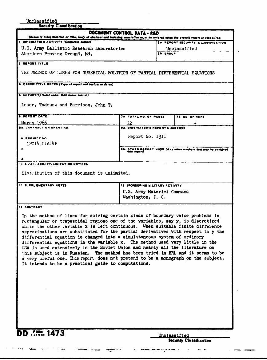
UnclassifiedSecurity Claification

DOCUMENT CONTROL DATA - R&D(Ieaguwty Claesiflatln elf tile. 411040 o e*W10 an d f nindeahg anntatin must he enteresd 0 0em os overell report is Cwealfied)

RI.ONI1NiTIN 0 ACTIVITY (Coomet samllr) 20-l REPOPRT SECURI TY C LASIFIICATION

U.S. Army Ballistic Research Laboratories• Unclassified

Aberdeen Proving Ground) Md. 2e GOUP

3. REPORT TITLE

THE METHOD OF LINES FOR NUMERICAL SOLUTION OF PARTIAL DIFFERENTIAL EQUATIONS

'4. DESCRIPTIvE NOTES (Type of rsepot and Incluelve date*)

I. AUTHOR(S) (Lost name. tint name, Initial)

Leser, Tadeusz and Harrison, John T.

6. •ElPORT DATE TOTAL NO. OF PAGES 7b. MC. or REFS

March 1.66 321 4Ga. CONTRA4.T OR GRANT IO. Ga. ORIGINATOR'S RIPORT Numsej"S)

. PROJECT NO Report No. 1311IPOi45OIA L4B _____________________

C Sb. &[TW.=PO NO(S) (Any o.9,r mas.es flat my be aee.G.ed

d.

'0. A VA IL. ADILITYV'LIITATIO4 NOTICES

Distribution of this document is unlimited.

I! SUPPL. EMENTANY NOTES 12 PONSORING MILITARY ACTIVITY

U.S. Army Materiel CommandWashington, D. C.

12 ABSTRACT

In the method of lines for solving certain kinds of boundary value problems inrL.ctangular or trapezoidal regions one of the variables, say y, is discretizedwhii. the other variable x is left continuous. When suitable finite differenceapproximations are substituted for the partial derivatives with respect to y thed ifferential equation is changed into a simulataneous system of ordinaryditferential equations in the variable x. The method used very little in theUSA is used extensively in the Soviet Union and nearly all the literature ont-his subject is in Russian. The method has been tried in BRL and it seems to bea very uzeful one. This report does nnt pretend to be a monograph on the subject.It intends to be a practical guide to computations.

DD 'i* 1473 UnclassfiedSecurty Claamfceadon

Uncl~assifiedSecurity Classification

KE WRD LINK A LINK 9 L11 K C

R____________ OLE *WY 4OLE 9 W ROL.E ft '

Partial Differential. EquationsNumerical Methods

INSErCTIONS

1. ORIGINATING ACTIVITY: Enter th. name an adrs 10. AVAILABILITY/LIMITATION NOTICES: Enter any Urn-of the contractor. subcontractor, grantee, Departmen of Do- itations on further dissemination of the report. other than thoselense activity or other organization (corporale author) issuingimoebyecryclsfctinusgsadadtamntthe report, much byscrt lsifcto.uigStnadsaeet

2a. REPI)RT SECUNTY CLASSIFICATION: Enter the over. (1) "Quaified requesters noay obtain copies of thisall security clissification of the report. Indicate whetherreotPriDC

"~ R.str&Ated Dsta" is includeL. Marking is to be in accpotrd- DC..arct withi aorpriate secrwity regulations. (2) "Foreign announcement and dissemination of this2h. G1it(UP: Aulumatic downgrading is specified in DOD Di report by DDC is not authtorized.'rvc t iv 520)O. 10 and Armed Forces Industrial Manual. Enter (23) 11U. S. Goverrnment agencies may obtain copies ofthti group number. Also, when applicable. show that optional this report directly from DDC. Other qualified DDCmarkints. have been used for Group 3 and Group 4 as author- users shall request throughired.

V 3 REPORT TITLE. Enter the complete report title in all (4) 1U. S. military agencies may obtain copies of thiscaopitat 'etters. Titles in all cases should be unclassified. report directly (mee DDC. Other qualified usersIf a meaningful title cannot be selected without classifiescwarqet hogtio n sh.:w titll classification in all capitals in parenthesissalreuttwohI m mediately following the title._____________________

4.DESCRIPTIVE NOTE&: If appopriate, enter the toor at (S) "All distribution of this report is controlled. Qual-report. e~g.. interim. progress. summary, annual. or final, diled DDC users soal request throughGave the inclusive dates when a Specific reporting period is a.4co'vered.ItterprhabenfrihdtthOfieoTenclS. AlIT NORS) Enter the roame(s) of &watho(*) aso showni on If the rDepeartmhsbento omre f ori"id to the Offbceco Teindi-a'r in the report. Enter last nmest. first name. midde intitiaL. cae tis, facttadenteoromec.fr aet the priclic nil-owIt. military. slow Taft and branch of servce. The same of a.tsfetaieerhepceifno.Ithe princspal author is an absiolute ainimum requirement. I L PPPLKMNTARY MOTEL Use for additional etiplerow6. REPORT DiATE: Ener toke date of the reo"t as day. t017 OHMm'-nth. year. or month. year. If oe than one dtew metso 1,2. UPOl @011WO MILITARY ACTIVIlTY: "ntr the nwame ofan the report. use date of publication. Ithe department project *Mie* er lrabtaory sponsoring (pey7U. TUTAL NtJM61E Of PAQIC The Itotl pag" count ins lot) the research sad development. Incluide sib.* Ill.should follow nramal pagination procedures. La.. enter the 13L AUSTNACT ante on abstract giving a brief and factualnumtoer of pages coroainttill i'smetioti, summary of the documtent 1ndaC01teve Of the repot. even th"%g

at "ay also appear elsewhere in the boady 0f the ltehnical roe76. NUMBER Of REFERKNCIM Enter the total WA6 Of Iport. If additional *paer is requred. a continuittleo Shootreferences cited in the report. shell be attached.Il.. CONTRACT ON CARANT NWERM If approptriae,. ente It is hilthly desirable that the abstract Of clas4ifie4 tothe applicable RUmber of the coaftecrt or great under which ports be unirlassified. Each pwaragrah Of the Abstract shaltthe report was mitten i end with an indlicationo of the military socuwity cla4msficetion1$6. or. b 3d. PROJECT 10I'tIsaM Enter the aftropriate, of the intonnsat inn in the paragraph. represented as (1S). (3).military dsporlIIeI idon.:6tc sties. Such aso projec~t wmbelr. (C). or (t))surbpootect modoor. sysbem numboer. tosk nuimbero. etc. There is no limitation one the length of the abstract. How-

9.. RIGNATO'S EPOR Nula(S Ener te *%obr. the suggested lenglth is from ISO to 225 "ordsctal torpet number by which the dwuouen will be identified 14. KEy 9011106 Key wnords ato technically metoalingul termssad cor"olled by the originmatin activity. Twos alero woat of short praews** that characteize a report alid maye be used nbe utiie to this report. des% entries for catalegtrig the reorot. Key waeds amust be96 yTI otherT NUepor 11.t tuha eubry ~hifte boos Selected so tha no security classkifce4"toe is rquird. 141e411assigned an te ae smee(01trb h 01~ fkiers Such as equipment mdodel de"gnatou. trade name. -silk,

A0 W000f. 600 @ar 111116 111114100166isry project rode name. geographic locaticia. way beo u~e as~V words but wilt be followed bv an indeaication .4gctmnical

conies The assignmoent of lninks. tiglet. OVA Weights to

Septionalifcaio