faculdade de engenharia da universidade do porto · 2017-08-28 · faculdade de engenharia da...
TRANSCRIPT
Faculdade de Engenharia da Universidade do Porto
Traction Control for Hybrid Electric Vehicles
José Ricardo Sousa Soares
Master Dissertation conducted within the Program of Integrated Master in Electrical and Computers Engineering
Branch: Automation
Supervisor: Adriano da Silva Carvalho
July, 2012

© José Ricardo Sousa Soares, 2012

To my mother, my brother and in memory of my father


i
Resumo
O objetivo da Dissertação é o desenvolvimento de um sistema de tração elétrico com
travagem regenerativa para a adaptação de uma moto quatro com motor de combustão para
um veículo híbrido série.
O documento apresenta o estado de arte da tecnologia em termos de veículos híbridos
com base na revisão bibliográfica realizada, com especial atenção nos seus subsistemas
diretamente relacionados com controlo de tração.
Neste documento são ainda especificados os problemas a tratar e as soluções
desenvolvidas para controlo e implementação em hardware são apresentadas.
A máquina a ser controlada é um motor síncrono de ímanes permanentes e assim sendo
são apresentados aspetos sobre o princípio de funcionamento da máquina assim como uma
análise sobre a definição de angulo de binário.
Vários métodos de controlo são discutidos e comparados com o objetivo de justificar a
melhor solução para o controlador de tração. O algoritmo de alto nível assim como a solução
para a plataforma de controlo para o sistema de controlo são também aspetos discutidos
neste documento.

ii

iii
Abstract
The scope of the Dissertation is the development of an electric traction system with
regenerative braking for the adaptation of a four-wheeled motorbike with an internal
combustion engine into a series hybrid electric vehicle.
The document presents the Technology State of the Art in the field of hybrid vehicles
based on a bibliographic review executed with special focus at subsystems directly related
with traction control.
In this document are also specified the issues to be analyzed and the developed solutions
for the control and hardware implementation.
The machine to be controlled is a PMSM and thus an overview of the PMSM working
principle is carried out as well as an analysis of the torque angle definition is discussed.
Several control methods are discussed and compared in order to justify the best solution
for the traction controller. The high level algorithm as well as the control platform for the
electric traction system are also subject of discussion in this document.

iv

v
Acknowledgements
I would like to thank my supervisor, Professor Adriano da Silva Carvalho, for all the
support and guidance during the development of the Dissertation, always promoting my self-
development giving not always the answers but always raising the right questions.
I must thank my teammate and friend Tiago Sá, for the many issues we discussed together
and the many exchanged viewpoints and information that helped the improvement of this
Dissertation.
I would like to acknowledge my friends, specially my fellow students, for all the
friendship, smiles and good disposition.
I would like to thank my family, particularly my brother and of course my mother whom I
am deeply grateful for all the sacrifices, the liberal and robust education, which I am proud
of, and for the important advices that pointed me in the right direction and made me a man.
At the end, but not less important I want to thank Daniela, for all the love, the support,
the words and patience and for being always there for me.

vi

vii
Contents
Resumo .............................................................................................. i
Abstract ............................................................................................ iii
Acknowledgements ............................................................................... v
Contents ........................................................................................... vii
List of Figures .................................................................................... xi
List of Tables ..................................................................................... xv
List of Acronyms ............................................................................... xvii
Chapter 1 ........................................................................................... 1
Introduction ....................................................................................................... 1
1.1. Scope of the Dissertation ............................................................................. 2
1.2. Concept .................................................................................................. 3
1.3. Requirements Analysis ................................................................................ 3
1.4. Dissertation Structure ................................................................................. 4
1.5. Conclusion ............................................................................................... 5
Chapter 2 ........................................................................................... 7
State of the Art .................................................................................................. 7
2.1. Hybrid Electric Vehicle Power Train Architecture ............................................... 7
2.1.1. Series Hybrid Electric Drive Train .............................................................. 8
2.2. Electric Machine ..................................................................................... 10
2.2.1. Induction Motor ................................................................................. 11
2.2.2. Permanent Magnet Motors .................................................................... 12
2.2.3. Switched Reluctance Motor ................................................................... 13
2.3. Power Converter ..................................................................................... 13
2.4. Control Approach .................................................................................... 14
2.5. Control Platform ..................................................................................... 15
2.5.1. DSP ................................................................................................ 15

viii
2.5.2. FPGA .............................................................................................. 16
2.5.3. Microcontroller .................................................................................. 17
2.6. Conclusion............................................................................................. 17
Chapter 3 .......................................................................................... 19
System Modeling ............................................................................................... 19
3.1. Permanent Magnet Synchronous Machines ...................................................... 19
3.1.1. Working Principle ............................................................................... 19
3.1.2. Dynamic modeling of a PMSM ................................................................. 21
3.1.3. Torque Angle .................................................................................... 25
3.2. Mechanical System .................................................................................. 30
3.3. PSIM Dynamic Model Simulation ................................................................... 30
3.4. Conclusion............................................................................................. 33
Chapter 4 .......................................................................................... 35
System Controller Design ..................................................................................... 35
4.1. Principles of Vector Control ....................................................................... 35
4.2. Traction Control Loop ............................................................................... 36
4.3. Traction Control Methods .......................................................................... 37
4.3.1. Current Angle Based Torque Control ........................................................ 37
4.3.2. Air Gap Flux Angle Based Torque Control .................................................. 39
4.3.3. Direct Torque Angle control .................................................................. 41
4.3.4. Maximum Torque Per Ampere Control ...................................................... 44
4.3.5. Regenerative Braking .......................................................................... 46
4.3.6. Start-Up .......................................................................................... 48
4.4. PI Controllers ......................................................................................... 48
4.5. Space Vector PWM ................................................................................... 49
4.6. Rotor position and Speed Computation .......................................................... 55
4.6.1. Sensorless Estimation .......................................................................... 55
4.6.2. Sensor Acquisition .............................................................................. 56
4.7. PSIM Torque Control System Simulation ......................................................... 58
4.8. High Level Control Algorithm ...................................................................... 61
4.8.1. Motoring action ................................................................................. 63
4.8.2. Energy Recovery ................................................................................ 63
4.9. Conclusion............................................................................................. 64
Chapter 5 .......................................................................................... 65
System Hardware Architecture and Description ......................................................... 65
5.1. Hardware Platform Overview ...................................................................... 65
5.2. Hardware Specification ............................................................................. 67
5.3. Hardware Architecture ............................................................................. 69
5.4. Conclusion............................................................................................. 70
Chapter 6 .......................................................................................... 71
Global Results .................................................................................................. 71

ix
6.1. Computational Simulation Results ................................................................ 71
6.2. Hardware Implementation Achievements ....................................................... 76
6.3. Conclusion ............................................................................................. 78
Chapter 7 .......................................................................................... 79
Conclusion ....................................................................................................... 79
7.1. Dissertation Conclusion ............................................................................. 79
7.2. Further Developments .............................................................................. 81
References ........................................................................................ 83

x
xi
List of Figures
Figure 1.1 - High level functional architecture of the system ......................................... 2
Figure 1.2 - Electric propulsion system architecture for the hybrid electric vehicle .............. 3
Figure 2.1 - Classification of HEVs: Series architecture in the left; Parallel architecture in the right [3] .............................................................................................. 7
Figure 2.2 - Configuration of a series hybrid electric drive train [6] ................................. 8
Figure 2.3 - Suitable characteristic for HEV [5] ........................................................ 10
Figure 2.4 - Different characteristics of induction motor [4] ........................................ 11
Figure 2.5 - Torque-Speed characteristic of a PM machine .......................................... 12
Figure 2.6 - Characteristic of a SRM [4] .................................................................. 13
Figure 2.7 - Basic circuit configuration of an inverter, adapted from [2] ......................... 14
Figure 2.8 - FPGA architecture [1] ........................................................................ 16
Figure 3.1 – Four-pole internal magnet motor with tangentially magnetized PMs in the left and radially magnetized PMs in the right [21] ................................................... 20
Figure 3.2 - Simplified equivalent circuit of the PMSM in the dq reference frame .............. 23
Figure 3.3 - Steady-state vector diagram of the PMSM in dq reference frame for a given working point, adapted from [21] .................................................................. 24
Figure 3.4 - Steady-state vector diagram of a PMSM in dq reference frame for a given working point of motor operation .................................................................. 26
Figure 3.5 - PSIM Block Schematic for Dynamic Modeling of a PMSM; Mechanical Load and Inverter ................................................................................................. 31
Figure 3.6 - Speed and Torque for both model and PSIM block ...................................... 32
Figure 3.7 - Torque and Torque Angle for a PMSM without control ................................. 32
Figure 4.1 - PMSM Control System Architecture ........................................................ 36
Figure 4.2 - Torque response; Stator phase currents and current angle for the Current Based Angle Torque Control ......................................................................... 38

xii
Figure 4.3 - Torque response; Stator phase currents and current angle for the Air Gap Flux Based Angle Torque Control ......................................................................... 40
Figure 4.4 - Torque response; Stator phase currents and current angle for the Air Gap Flux Based Angle Torque Control with an id ramp reference ....................................... 41
Figure 4.5 - Torque response; Stator phase currents and current angle for the Direct Torque Angle Control ................................................................................. 43
Figure 4.6 - Torque response; Stator phase currents and current angle for the Maximum Torque per Ampere Control ......................................................................... 45
Figure 4.7 - Steady-state vector diagram of a PMSM in dq reference frame for a given working point of generator operation ............................................................. 46
Figure 4.8 - Regenerative Braking operation ........................................................... 47
Figure 4.9 - Stator current phase, air gap flux phase and stator voltage phase for motoring and regenerative operation ......................................................................... 47
Figure 4.10 - Space vectors of a three-phase bridge inverter (adapted from [26]).............. 51
Figure 4.11 - Sequence timing generation stages ...................................................... 53
Figure 4.12 - PSIM block schematic for the Space Vector PWM algorithm ......................... 54
Figure 4.13 - Phase voltages of phase a, b and c ...................................................... 54
Figure 4.14 - Position and Speed Computation Block implemented in PSIM (left) and the respective speed and position signals for motoring operation (right) ....................... 58
Figure 4.15 - Control and power system implemented in PSIM ...................................... 59
Figure 4.16 - PERM 156 Air Gap Flux Angle Based Torque Control .................................. 60
Figure 4.17 - PERM 156 Direct Torque Angle Control .................................................. 60
Figure 4.18 - PERM 156 Current Angle Based Torque Control ........................................ 61
Figure 4.19 - High level algorithm ........................................................................ 62
Figure 5.1 - FPGA based platform with the soft processor MicroBlaze ............................. 66
Figure 5.2 - Block diagram of Hybrid Kit for HybridPACK™1[31] .................................... 66
Figure 5.3 - Infineon Hybrid Pack 1....................................................................... 68
Figure 5.4 - Software into hardware mapping .......................................................... 69
Figure 6.1 - PERM 156 relevant quantities for constant torque reference and variant torque load ............................................................................................. 72
Figure 6.2 - PERM 156 relevant quantities for variant torque reference and constant torque load ............................................................................................. 73
Figure 6.3 - PERM 156 relevant quantities for variant torque reference and variant torque load ...................................................................................................... 73

xiii
Figure 6.4 - PERM 156 relevant quantities for variant torque reference and constant load torque in reverse direction .......................................................................... 74
Figure 6.5 - PERM 156 relevant quantities for regenerative braking operation .................. 75
Figure 6.6 - PERM 156 relevant quantities for motor operation and regenerative braking operation ............................................................................................... 75
Figure 6.7 - Traction control algorithm developed in Matlab Simulink ............................ 76
Figure 6.8 - Space Vector computation subsystem implemented in Matlab Simulink ........... 77

xiv

xv
List of Tables
Table 1.1 - Main characteristics of the vehicle, adapted from [7] ................................... 2
Table 1.2 - Document structure ............................................................................. 4
Table 2.1 - Operative modes of a series electric hybrid vehicle, adapted from [3] ............... 9
Table 4.1 – Three Phase Inverter Switching Vector States ........................................... 50
Table 4.2 - Lookup Tables for the three top inverter switches ...................................... 54
Table 4.3 - Relevant parameters for the control simulation of the PERM 156 PM motor ....... 58
Table 5.1 – Motor parameters from PERM 156 datasheet ............................................. 67

xvi

xvii
List of Acronyms
AC Alternated Current
BLDC Brushless Direct Current
CPU Central Processing Unit
DC Direct Current
DSP Digital Signal Processor
ECU Engine Control Unit
EMF Electromotive Force
FOC Filed Orientation Control
FPGA Field Programmable Gate Array
HDL Hardware Description Language
HEV Hybrid Electric Vehicle
ICE Internal Combustion Engine
IGBT Insulated Gate Bipolar Transistor
IM Induction Motor
ISE Integrated Software Environment
OTP One Time Programmable
PI Proportional-Integral Controller
PLL Phase-locked Loop
PM Permanent Magnet
PMSM Permanent Magnet Synchronous Machine
SRAM Static Random Access Memory
SRM Switched Reluctance Motor
VHDL VHSIC Hardware Description Language
VHSIC Very High Speed Integrated Circuits
XPS Xilinx Platform Studio
A/D Analog to Digital Converter

xviii
List of symbols
Friction coefficient
Direct axis back EMF component
Quadrature axis back EMF component
EMF created by the permanent magnets
(t) Input error of the PI controller
Current of phase a
Current of phase b
Current of phase c
Direct axis current component
Quadrature axis current component
Stator current vector
Stator current amplitude
Moment of inertia
Proportional gain of the PI controller
Ratio between motor poles and resolver poles
Direct axis inductance
Quadrature axis inductance
Stator phase inductance
p Machine pole pairs
P Active Power
Stator phase resistance
Electromagnetic Torque
Load Torque
Shaft time constant
Integral time
Space Vector Modulation carrier wave period
Voltage of phase a
Voltage of phase b
Voltage of phase c
Direct axis stator voltage component
Quadrature axis stator voltage component
Alpha axis stator voltage component
Beta axis stator voltage component
Stator voltage amplitude
Stator voltage amplitude for Space Vector Modulation computation
Stator voltage phase for Space Vector Modulation computation

xix
Electric position with respect to d-axis
Stator voltage phase angle
Stator current phase angle
Air gap flux linkages phase angle
Phase angle between stator voltage vector and EMF
Torque angle from definition
Flux linkage of phase a
Flux linkage of phase b
Flux linkage of phase c
Direct axis air gap flux vector component
Quadrature axis air gap flux vector component
Flux linkages proper of the rotor permanent magnets
Air gap flux linkages vector
Air gap flux linkages amplitude
Electrical system angular speed
Mechanical angular speed

xx

Chapter 1
Introduction
Millions of vehicles circulate in the roads every day. They satisfy most of society mobility
needs because they are comfortable, flexible and convenient. The internal combustion engine
was a remarkable discovery and the fast development of automotive industry made the
internal combustion engine vehicle an amazing piece of technology in the present days.
However, internal combustion engines produce toxic gases as a result of their operation.
These toxic gases have caused and continue to cause serious problems for environment and
human life.
With the fast increase of car ownership, environmental concerns as air pollution, global
warming, and the rapid depletion of the Earth petroleum resources have become a matter of
attention all over the world. In order to ensure the quality of environment and human living
life the automobile industry has started many researches in the area of vehicles based on
electric propulsion. Electric propulsion vehicles have such promising advantages as high
efficiency and zero emissions. However, a major disadvantage of pure electric vehicles
compared to vehicles ran by fuel is their low autonomy range.
High density power battery energy storage systems are a great achievement of today’s
technology and their improvement is increasing quickly, although it is very difficult to reach
the autonomy range of an internal combustion engine vehicle. Hence, the market trend is
evolving in the direction of the hybrid electric vehicles where a second source of energy
provides power for an extended autonomy range.
Being the electric mobility emerging in the market many researches are going on aiming
to improve the electric and hybrid electric technologies. Hence, the scope of the Master
Dissertation conducted on behalf of the Program of Integrated Master of Electrical and
Computers Engineering is the development of an electric traction system unit to integrate a
hybrid electric vehicle.
This document presents the discussion about the problem that the Dissertation pretends
to solve as well as its development and results. In this very first chapter, it is more detailed
explained the context and the scope of the Dissertation as well as the structure of the

2 Introduction
present document. In the second chapter is exposed the State of the Art of hybrid electric
vehicles.
The third chapter presents the system modeling as well the working principle of
permanent magnet synchronous machines and in the fourth chapter is presented the system
controller design to control the motor.
The fifth chapter presents the system architecture and finally the sixth chapter presents
the overall results from the computational simulations till the hardware implementation
achievements.
Finally, in the seventh chapter the conclusions and future work to develop are presented
and discussed.
1.1. Scope of the Dissertation
This Dissertation presents the outcomes from one stage of a larger project that consists in
the adaptation of a regular four-wheeled motorcycle with an internal combustion engine in a
series hybrid electric vehicle. The vehicle in question is a Honda Fourtrax propelled by a 12
kW four stroke internal combustion engine. The main characteristics of the vehicle are
summarized in the next table:
Table 1.1 - Main characteristics of the vehicle, adapted from [7]
Model: HONDA trx 250tmb
Engine: 229cc four-stroke, air cooling
Dimensions: 1,9m x 1,035m x 1,17m
Weight: 196 Kg
There are mainly three sub-systems to have in account for the adaptation of this vehicle:
the traction control unit; the energy management control unit; and the IEC-generator control
unit. A functional architecture diagram for the system is represented in the next figure:
The scope of the Dissertation relies on the development of the electric traction control
unit for the hybrid electric vehicle.
During its development, the system has to be modeled and simulated, in terms of dynamic
response in appropriated simulation software. After simulation, the sub-systems as in the
inverter and the control platform have to be coupled to the motor.
Figure 1.1 - High level functional architecture of the system

Concept 3
3
1.2. Concept
In this section is presented the concept and architecture of the proposed problem. The
traction control unit has three main components: the electric machine; the power inverter
and the controller.
The control platform for the system implementation is also an issue of the Dissertation
scope that is going to be discussed throughout this document. The next figure shows a
schematic of the concept architecture for the electric propulsion system of the hybrid
electric vehicle:
The controller receives the reference signal from both the throttle and the brake and
processes it in order to obtain an error signal that results from the difference of what is
expected and what is being produced. The error signal is computed with a vector control
algorithm that also measures the phase currents of the motor to close the current control
loop. Then the PWM signals to drive the gates of the inverter switches are generated.
There is also a communication link with the energy system management control so that
the control system can be aware of the energy and power available for traction or to be
aware of whether is possible to recover energy or not.
1.3. Requirements Analysis
When a vehicle is developed it has to meet not just the performance and comfort
requirements but more importantly there are security requirements to be ensured.
As a matter of performance, the control must be complete enough to respond to an input
signal from the throttle and satisfy the expected acceleration and speed required by the
driver.
Concerning the efficiency of the vehicle the system must be capable of recovering energy
to the DC bus in case of braking or deceleration. During deceleration the energy recovery
process must be slow and smooth being imperceptible for the driver. During braking the level
Figure 1.2 - Electric propulsion system architecture for the hybrid electric vehicle

4 Introduction
of energy recovered has to be progressive and proportional to the position of the brake
actuator.
Regarding of security the electric brake must be reliable to ensure that the vehicle is
going to stop within a short distance. Furthermore, the electric brake must be completed
with a mechanical brake operating within an embedded approach to ensure that if the
regenerative control fails the mechanical brake will do its job and decelerate the vehicle
safely. Another security aspect that needs to be ensured is related with the level of energy
that can be recovered. If the energy management control unit gives the information that
there is no possibility to recover the energy from breaking, then the system has to decide to
damp the energy in a power resistor otherwise the amount of energy could be cause hazard to
the system.
1.4. Dissertation Structure
The present document integrates all of the work developed, as well as the results and the
conclusions obtained.
It is presented in table 1.2 the structure of this document:
Table 1.2 - Document structure
Chapter Description
Chapter 1. Introduction Description of the Dissertation scope and
context.
Chapter 2. State of the Art Bibliographic review and State of the Art
for HEV technology.
Chapter 3. System Modeling
Description of the working principle of
permanents magnet synchronous machines
and dynamic modeling of the system
regarding its mathematical equations as
well as its simulations developed with
simulation tools.
Chapter 4. System Controller Design
Presentation and description of developed
control methods and computational results
comparison regarding of the controller
design
Chapter 5. Hardware Architecture
. and description
Description of the technical aspects
concerning the implementation of the
control algorithm in the control platform.
Chapter 6. Overall Results
Discussion of the global results for
computational simulations and hardware
implementation achievements.
Chapter 7. Conclusions Conclusion and discussion about further
developments

Conclusion 5
1.5. Conclusion
This chapter introduces the context and the scope of the Dissertation. It is presented and
described the concept of the system as well as its requirement analysis. Finally the structure
of the document is stated.
This chapter aims to expose the proposed problem of the Dissertation and how is the
solution be treated and developed. The following chapter presents a bibliographic review and
state of the art for HEV technologies.

6 Introduction

Chapter 2
State of the Art
This chapter presents the State of the Art of hybrid electric vehicle technologies
presenting an overview about its architecture and its subsystems based on a bibliographic
review.
2.1. Hybrid Electric Vehicle Power Train Architecture
Considering that a hybrid vehicle has more than one source of energy it is very important
to analyze the structure of the connections between the components that define the energy
flow routes in order to give power to wheels. In a hybrid electric vehicle one of the energy
sources is naturally electric energy, stored in a high density power battery and the second
source is, in this case, based on the energy density of fuel that operates an ICE to generate
electric power.
There are two main architectures of HEV power train: series and parallel one. The
classification depends on how the energy coupling is done. To understand the differences
between these two main architectures it is presented in figure 2.1 the architecture of both
serial and parallel architectures.
Figure 2.1 - Classification of HEVs: Series architecture in the left; Parallel architecture in the right [3]

8 State of the Art
In the series hybrid drive train the ICE is fed with fuel and is mechanically coupled to a
generator that produces electric energy from the fuel and delivers electric power to a power
converter which adapts power waveform to DC power connecting it to the DC bus. In this
architecture the energy coupling is done at the power converter level so it is called electric
coupling. The two electrical powers (from the battery and from de generator) are added
together and the power flow is controlled and delivered to the electric motor, or also in the
reverse direction in case of regenerative breaking, from the electric motor to the battery.
On the other hand, in the parallel architecture the mechanical power from the ICE and
the mechanical power from the electric motor, fed by the battery through the power
converter, are added together at the mechanical coupler. In this case, the power flow can be
controlled only by the engine and the electric motor connected to the mechanical coupling.
2.1.1. Series Hybrid Electric Drive Train
The architecture proposed for the target vehicle of this Dissertation is the series hybrid
electric architecture which will be discussed here with more detail.
The series hybrid architecture drive train has two electric power sources, one of them is
the battery which is bidirectional and the other one, which is unidirectional, is a fuel tank
that feeds an ICE coupled to an electric generator. Both sources of energy feed a single
electrical machine that propels the vehicle [6].
The power coupling of the two sources is done at the DC link level, and so it is called
electrical coupler as is said above. In order to easily understand this architecture it is
represented in figure 2.2 a schematic representation of the main components that integrate
the series hybrid electric drive train.
As is represented, the voltage from the generator is rectified and delivered to the DC link
through a unidirectional rectifier. On the other hand, the battery pack is connected to the
same DC link through a bidirectional DC/DC converter which makes the voltage level interface
between the DC link voltage and the battery pack voltage.
Figure 2.2 - Configuration of a series hybrid electric drive train [6]

Hybrid Electric Vehicle Power Train Architecture 9
Hence, the power from both energy sources is delivered to the electrical motor by means
of this DC link which feeds the controlled power inverter that drives the electric motor.
Naturally, in case of regenerative breaking the controlled power inverter is also responsible
to rectify the current produced by the motor and deliver it to the DC link bus. The problem
respecting the energy recovery is that if a large amount of energy is produced in a relatively
small period of time it produces peaks of current that may cause hazard to the battery’s
health. A good solution to avoid this problem is the utilization of an ultra-capacitor storage
system in parallel with the battery pack. Ultra-capacitors can handle transient operations
efficiently and thus absorb the current peaks due to hard breaking situations [8]. On the other
hand, the energy stored in the ultra-capacitors may then be used for a fast acceleration
which requires an instantaneous large amount of power.
The utilization of this ultra-capacitor storage system may provide not just a solution to
the transient aspects of the regenerative energy recovery but also increases the vehicle
performance as well as the battery life time.
However, the power flow at the DC link level must be precisely controlled to ensure the
vehicle performance and security. The control of the DC link power flow is addressed to the
energy management system unit which must inform the traction control of the power
available for traction as well as whenever the energy recovery if possible or not.
This type of architecture is normally associated to seven operative modes. The next table
describes these seven modes of operation:
Table 2.1 - Operative modes of a series electric hybrid vehicle, adapted from [3]
Operative Mode Description
Pure electric mode The energy comes from the batteries and the
engine is turned off
Pure engine mode
The energy comes from the engine-generator
and the battery neither supply nor accept
energy
Hybrid traction mode The energy comes from both engine-
generator and batteries
Engine traction with battery charging mode
The power supplied by the engine-generator
propels the vehicle and charge the batteries
at the same time
Regenerative breaking mode
The power from the motor during braking is
used to charge the batteries and the engine is
turned off
Battery charging mode
The electric traction motor does not receive
any energy and the engine-generator only
charges the battery
Hybrid battery charging mode During braking situations both traction motor
and engine-generator charge the battery

10 State of the Art
In this architecture the traction control is similar to the traction control of a pure electric
vehicle, being simpler than the control in the parallel architecture, because the electric
machine is the main propulsion motor and there is no mechanical connection between the
engine and the transmission. Furthermore, since there is no mechanical connection between
the engine and the transmission, the engine can be operated always within its maximum
efficiency. Hence, low fuel consumption and low emission level can be achieved.
However, there is a disadvantage addressed to this architecture, since the energy from
the engine has to change its form twice, mechanical to electrical in the generator and
electrical to mechanical in the electric motor, the inefficiencies of the generator and the
traction motor as well as the power converters may cause significant losses. Thus, it is crucial
to have a very efficient control of the power flow at the DC link level.
2.2. Electric Machine
In this section is presented the typical electric motor topologies most used for electrical
traction in hybrid electric vehicles.
Regarding the HEVs operation and differing from industrial applications, the electric
motors will be exposed to continuous start and stop conditions, high rates of acceleration or
deceleration and a very large speed range of operation [9]. Thus, there are a certain number
of requirements for the electric motor regarding electric propulsion.
First of all, the electric machine must have a high instant power and high power density
together with high torque at low speeds for starting and climbing as well as high power at
high speed cruising. A very wide speed range and instant torque response are another to
important requirements. Then, it is also important that the electric drive has a high
efficiency over wide speed and torque ranges, high efficiency regenerative braking and, of
course, high reliability and robustness for many different operating conditions [10].
To illustrate the suitable characteristic of an electric motor in the field of HEVs it is
represented in figure 2.3 the expected torque-speed and power-speed characteristic for this
specific application.
There are two types of motor drives, the commutator motors and the commutatorless
motors. The commutator motors are the traditional DC motors, they have a very simple
Figure 2.3 - Suitable characteristic for HEV [5]

Electric Machine 11
control but they have a low specific power density and the need of brushes makes them
maintenance dependent and thus less reliable. These drawbacks of DC motors are making
them less attractive for HEVs applications.
On the other hand, the so called commutatorless motor drives like the induction motor,
the permanent magnet brushless motors and the switched reluctance motors are the most
used electric machines in hybrid vehicles because of their advantages as in higher efficiency,
higher power density, lower operating cost, maintenance-free and reliability when compared
with DC machines. Hence, the commutatorless machines have become really attractive
concerning the electric propulsion in HEV[3].
It will be explained further the main characteristics of this motor drives in order to find
the proper solution for the concern of this project.
2.2.1. Induction Motor
The induction motor is well known because of its simple construction, high power density,
reliability, ruggedness, low maintenance, low cost and ability to operate in hostile
environments.
When an advanced control method is used, it is possible to decouple the induction motor
torque from field control. Furthermore, speed range may be extended beyond base speed
using flux weakening in the constant power region [5]. In figure 2.4 is presented a diagram
with the characteristics of the induction motor.
However, there are some shortcomings of induction motors in comparison to PM motors
and SR motors. The existence of break-down torque in the constant power region, the
reduction of efficiency and increment of losses at high speeds, together with the low power
factor are the most critical [4].
In the perspective of HEVs, the shortcomings of the induction motor may have a
considerable impact on the vehicle’s performance but on the other hand it still has important
advantages for this application.
Figure 2.4 - Different characteristics of induction motor [4]

12 State of the Art
2.2.2. Permanent Magnet Motors
The PM machine is the result of replacing the field winding of conventional synchronous
motors with permanent magnets. This way the conventional brushes, slip-rings and thus field
losses are eliminated.
These machines are generally classified on the basis of the shape of their induced EMF
which can be sinusoidal or trapezoidal. The sinusoidal type is known as permanent magnet
synchronous machine or PMSM for short and the trapezoidal type is known as permanent
magnet brushless DC machine or simply BLDC [2]. In BLDC drives, the phase current
waveforms are rectangular, while in PMSMs the phase current waveforms are rather sinusoidal
ones.
To control brushless machines, rotor position information is needed. In the case of BLDC
the phase currents just have to be turned on and off, thus a low-cost hall sensor is enough. In
the case of PMSM drives, the phase currents waveforms need to be precisely controlled which
requires a high-cost position sensor. However, there are a few sensorless control techniques
based on position estimation that have been developed for both BLDC and PMSM drives [6].
The main advantages of PM machines are naturally related with the usage of permanent
magnets, since the magnetic field is excited by high-energy PMs, the overall weight and
volume can be significantly reduced for a given output torque, resulting in higher torque
density, and as mentioned above, with the absence of rotor winding there are no rotor copper
losses and thus an inherently higher efficiency than that of induction motor is achieved.
The torque-speed characteristic of a PM machine is represented in the following figure:
A drawback of the PM motor is its short constant power range due to its limited capability
for field weakening, resulting from the presence of the field created by the PM which can be
only weakened through production of a stator field component that is going to oppose the
magnetic field of the rotor [11].
Figure 2.5 - Torque-Speed characteristic of a PM machine

Electric Machine 13
2.2.3. Switched Reluctance Motor
Switched reluctance motors are becoming attractive in HEV systems every day mostly
because their torque-speed characteristic is very close to the suitable characteristic for
vehicle traction. Furthermore, their simple and robust construction, fault tolerance, simple
control and ability of extremely high speed operation are other important advantages of SR
machines regarding HEV applications [4].
The most advantageous characteristic of these machines is their ability to operate with an
extremely long constant power range, which is what makes this kind of machines very
suitable for hybrid electric vehicles applications [12]. To demonstrate this fact, it is
represented in the next figure the Torque-Speed characteristic of a SRM, and as it is possible
to show, the characteristic is very close to the expected one, presented above:
The main disadvantages of SRM are related with the high torque ripple of these machines
and also the acoustic noise produced by them. Although, there are many researches going on
regarding the reduction of the torque ripple and acoustic noise to an acceptable level for
vehicle application [11].
Another concern to have in account especially in this kind of machine is the shape of the
rotor. It should be optimally designed in order to reduce the high aerodynamic drag at high
speeds.
2.3. Power Converter
A DC/AC converter is a power converter that converts direct current into alternating
current. The converted AC current can have a voltage level that depends on the voltage at
the DC side and the frequency depends on the frequency imposed by the controller.
These DC/AC power converters are also known as inverters and they are of two main
types, depending on the type of the input. If the input is of constant voltage it is called
voltage-source inverter, in the case the input is of constant current then it is called current-
Figure 2.6 - Characteristic of a SRM [4]

14 State of the Art
source inverter. The power switches that integrate the inverter may be of many kinds
depending on the power level required [13].
According to its topology the inverter may have several voltage levels. They may be single
or multiphase and allow for bi-directional power flow. The energy retrieved from the motor
has to be either returned to the source, which in this case will be the batteries, or damped in
a power resistor when the battery and the ultra-capacitors are full. The fact that the energy
has to be dissipated in the resistor does not necessarily mean that this energy will be wasted
since the thermal energy produced in the resistor may be used for comfort purposes.
Figure 2.7 represents the basic configuration of a power inverter with the integration of
the regenerative circuit:
This basic power inverter has one leg connected to each phase of the electric machine, in
figure above is represented the circuit of a three phase inverter. The regenerative circuit has
also a switch that allows the current flow to the resistor when it is needed for the purposes
described above. The DC link filter provides a DC voltage level as constant as possible in the
DC link.
2.4. Control Approach
There are two main approaches for electric motor control, the scalar control strategies
and the vector control strategies. The scalar control strategies utilize the stator phase
current magnitude and frequency but they do not use their phases. This results in a deviation
of the phase and magnitudes of the air gap flux linkages from their set values. The
consequence of this deviation is that electromagnetic torque and speed oscillations will occur
and thus poor dynamic response will be achieved.
In the matter of HEVs applications a very good dynamic response is required and this
means that the variations in the flux linkages have to be controlled by the magnitude and
frequency of the stator and rotor phase currents and their instantaneous phases. This control
can be achieved by means of vector control [2]. The principle of vector control is described in
the chapter 4.
Figure 2.7 - Basic circuit configuration of an inverter, adapted from [2]

Control Platform 15
2.5. Control Platform
The control platform constitutes another concern of this Dissertation because high
performance control of the electric drive is complex and requires high processing capability,
multitask processing and high speed. Parallel processing or some high level algorithm task
scheduling is expected since the powertrain control involves the control of many different
modules regarding both performance and security at the same time.
There are a few platforms used nowadays for the powertrain control of an electric
propulsion system regarding of HEVs. Among the many solutions available, the most common
are based in DSPs (Digital Signal Processor), FPGAs (Field-Programmable Gate Array) and
microcontrollers already very used in automobile engine control systems. It will be stated in
this section the characteristics of these control platforms and discussed what they have to
offer concerning electric propulsion systems control.
2.5.1. DSP
A DSP (Digital Signal Processor) is a processor specially developed with the concern of
signal processing applications, like signal convolution, discrete Fourier transform, finite
impulse filter and so on. The DSP is developed to be small, to have low power consumption
and to be a low cost device. So, the key issues in DSP system design are power consumption,
processing power, reliability and efficiency.
The preferred programing language to code algorithms in a DSP nowadays is the C
language where fixed- and floating-point processing is used [14]. The utilization of DSP in the
field of automotive control is growing up very quickly and is replacing the regular micro-
processors because it exhibits high-speed performance, and combines peripheral circuits,
memory, and an optimized CPU structure on a single chip [15] which means that all the
hardware is available and the programmer just need to focus in the software development.
This fact makes DSP based systems less complex when compared with FPGA based systems,
the reason for that will be discussed later.
In the motor drive viewpoint, DSP has allowed the implementation of complex control
algorithms making possible for electrical machines to deliver their maximum performance
possible concerning torque-speed characteristics as well as dynamic behavior [16].
A particular and crucial drawback of DSP based systems is their difficulty to respond to
functional and timing specifications that vehicular applications require, concerning
performance and mainly security aspects. This problem is directly related with the sequential
processing approach of DSP architecture, this architecture decreases the controller bandwidth
when the solution needs to incorporate complex and time critical and so making DSP based
system non-deterministic which may compromise the timing specifications. The solution to
deal with this problem relies in the development of complex high level scheduling algorithms
to handle security time-critical aspects or, on the other hand with utilization of multi-core
DSPs, however the last one comes with a higher cost and integration complexity effort [17].

16 State of the Art
2.5.2. FPGA
An FPGA, in opposition to a DSP, is a regular structure of logic cells and interconnections
under complete control. This means that it is possible to interconnect these cells and design a
hardware circuit to implement the control algorithm. It is possible to program the interaction
between the cells and configure the FPGA using a hardware description language like Verilog
or VHDL.
The internal architecture of an FPGA is represented in figure 2.8:
There are two basic kinds of FPGAs: SRAM-based reprogrammable and OTP (One Time
Programmable). The SRAM FPGA is the most common one and can be reprogramed as many
times as it is needed. This kind of FPGA needs a system memory to store the data so it can be
reprogrammed each time it is powered up.
The OTP FPGA uses anti-fuses to make permanent connections in the chip, it does not
require a system memory to download the program, however if a change to the program is
needed after programming it, the chip has to be substituted [1].
Compared with a DSP, in a FPGA it is programed not just the software but mainly the
hardware, and that’s the reason FPGA have one level of complexity higher than DSP. This fact
can be a drawback because the solution for the same problem will probably take more time,
but on the other hand it comes with many advantages as in performance scaling, together
with the design integration and flexibility, since it is possible to design many blocks or multi
processors capable of running in parallel and integrate them in the same chip for high
performance and scalability. This functionality also provides deterministic latency which is a
crucial advantage when there are security concerns in a system [18].
The main disadvantage of programing hardware is the fixed point architecture. Vector
control requires floating point mathematical computation which can be difficult to implement
in the fixed point architecture of the FPGA. The fixed point architecture requires divisions
and products by multiples of 2 and this is a problem when math functions as square roots and
trigonometric functions are needed. In order to solve this problem an additional attention has
to be paid to implement a solution able to deal with floating point operations.
Figure 2.8 - FPGA architecture [1]

Control Platform 17
On the other hand, the mathematical space vector control algorithms are quite complex
and running them at high speed requires significant processing capabilities which can be
provided by the FPGA architecture and despites that it is also possible to design security
algorithms to run in parallel without affecting the main loop control algorithm which is not
possible to do with the serial processing architecture of a DSP.
Another relevant aspect directly related with this application is the constant need of
measuring analogic signals like the stator phase currents of the electrical machine, the FPGA
based hardware provides a significant increment in the sampling frequency of the current
control loop compared to the DSP based control system [19].
From the point of view of performance and computational capability, the FPGA platform
is preferred for the implementation of the electric powertrain control algorithm concerning
the aim of this Dissertation, although with the present concern of implementing a solution for
the fixed point math operations needed.
2.5.3. Microcontroller
Another solution is the microcontroller. Nowadays, microcontrollers are widely used for
many applications. As matter of fact, a microcontroller is already very used in ECUs or engine
control units in internal combustion engines.
Microcontrollers are small computers that integrate in a simple circuit a processor core, a
memory and also inputs and outputs and like the DSP, the microcontroller is normally
programed in C language.
In the present days there are microcontrollers designed with a high computing capability
running at hundreds of megahertz that allows complex mathematical calculations like the
ones required for vector control. Microcontrollers are normally developed specifically for
determined embedded systems which mean that the market offers microcontroller based
solutions already designed for motor control purposes. This fact facilitates and accelerates
the implementation of a system comparing for example with an FPGA where it is needed to
write the system code from the scratch.
Microcontrollers are normally a cheap solution and consume a low amount of power which
is also an advantage considering the nature of electric or hybrid electric applications. Hence,
a microcontroller based platform is also a good solution for the implementation of the system
controller.
2.6. Conclusion
This chapter presented the Stated of the Art technologies for electric and hybrid electric
vehicles and its architectures and subsystems based on a bibliographic review. The analysis
focused on the different types of electric machines, the inverter and the several solutions for
the controller platform in order to introduce the recent technology used in the field of
electric and hybrid electric vehicles.
The following chapter describes the dynamic modeling of the system considering the
working principle of the permanent magnet synchronous machine.

18 State of the Art

Chapter 3
System Modeling
The permanent magnet synchronous machine or PMSM for short is the type of electrical
machine chosen for this project. Their many advantages introduced in the State of the Art
chapter make these electrical machines very suitable for HEV applications.
In this chapter, it is explained the dynamic modeling for this type of machines as well as
its working principle. The understanding of the working principle and the dynamic model of
the machine are crucial aspects from the control point of view.
3.1. Permanent Magnet Synchronous Machines
3.1.1. Working Principle
The permanent magnet synchronous machine is a particular type of synchronous
machines. Synchronous machines are called this way because their speed is proportional to
the frequency of the source that feeds them. Hence, the speed of the machine is function of
the source speed as follows:
(3.1)
In other words, a machine connected to a source will run in synchronism with that source
and its speed will depend on its number of pole pairs.
The stator winding is the input winding when the machine is working as a motor, when
three-phase currents flow in the windings, magnetic poles are created on the surface of the
stator. These created pole pairs are moving along the stator surface, producing a rotating
magnetic field as the phase currents alternate in time sequence with a displacement of 120º
between them [20]. The rotor poles are created by permanent magnets in this kind of
synchronous machines in opposite to regular synchronous machines that use DC currents

20 System Modeling
flowing in the rotor field coils, this way there are no copper losses in the rotor and the overall
efficiency is improved.
The magnetic field produced by the rotor follows the rotating magnetic field created by
the stator and the shaft rotates in synchronism with the electrical system. The interaction
between the rotor flux and the stator current creates torque that varies as function of its
angular displacement.
The rotor of PMSMs may have different configurations which will lead to different
parameters in the characteristic equations as it will be discussed further. The different
topologies of these machines are classified according to the displacement of the PMs in the
rotor. The motors can have surface-mounted PM, inset PM or interior PM. In the case of
surface-mounted PMs, the PM are mounted on the surface of the rotor with alternating
polarity, in the case of the inset mounted the situation is similar to the surfaced-mounted
apart of an iron tooth between each permanent magnet. The permeability of the PMs is
closed to the air so the surface-mounted motors have an isotropic rotor which means that the
flux is uniform in all orientations. On the other side, the inset PM rotors have a moderated
anisotropy created by the iron teeth.
Anisotropy of the rotor leads to two components of torque: the PM excitation torque and
the reluctance torque. An interior PM motor have a high rotor anisotropy, the two
components are high, hence the interior PM rotor have a high torque. [21].
The interior PM motors can be classified in radially magnetized PMs or tangentially
magnetized PMs according to the direction of the magnetization of the PMs inside the rotor.
In the next figure it is possible to analyze and distinguish the two types of magnetization:
Figure 3.1 – Four-pole internal magnet motor with tangentially magnetized PMs in the left and radially magnetized PMs in the right [21]
With PMs having tangential magnetization and the polarity alternated, the flux in the air
gap is the sum of the flux of two PMs. Motors with rotors of this type are normally build with
higher number of poles in order to produce a higher concentration of flux in the air gap
because with more poles the sum of the surface of two PMs is higher than the pole surface.
[21]

Permanent Magnet Synchronous Machines 21
In the case of the figure 3.1 in the right, the PMs have alternating polarity as well, but
this time the PMs have radial magnetization. With this type of configuration, the flux density
in the air gap is lower because the PM surface is also lower than the pole surface.
Either tangential magnetized or radial magnetized PMs will lead to high rotor anisotropy.
All of the rotors have magnetic paths with different permeance which gives them the
possibility of developing a reluctance torque component.
In figure 3.1, it is shown that a two axes system is used, the d-axis is called the direct axis
and the q-axis is called the quadrature axis. The two axes are 90º electrical degrees shifted
which corresponds to 45º mechanical degrees as it is shown in the figure due to the number of
machine poles. The use of this axes system will be explained further, but it is important to
notice here that d-axis inductance results to be lower than the q-axis inductance for the case
of internal permanent magnet rotors because they present paths with different permeance, in
opposition to the surface mounted rotors that have equal permeance in both axis since the
permeability of the permanent magnet is close to the permeability of the air. Hence, the
anisotropy or saliency ratio is defined as the following ratio: [21]. This relation
between the inductances is an important variable to have in account from the point of view
of control because it affects the torque production of the motor as it will be shown further.
3.1.2. Dynamic modeling of a PMSM
In order to develop an efficient control for the electric drive an analysis of the machine
from a dynamic point of view is necessary. The dynamic model of an electrical machine is
derived by using a two-phase motor which provides simplicity when treating an n-phase
machine by representing it in its two phase equivalent. This approach results in the
representation of all of the motor electrical quantities in a system of two axes [2].
The two axes system can be stationary, which is called the αβ reference frame, or
rotating which is called dq reference frame. Both reference frames can be used to
dynamically model the machine being the rotating reference frame the most used from the
control point of view since the frame is rotating synchronously with the rotor and the electric
quantities are constant in steady state contrarily to the stationary reference frame where the
quantities are sinusoidal in time.
The PMSM can be modeled in the orthogonal stationary reference frame αβ by projecting
the three phase quantities in the two axes which results in the following transformation:
[
]
[ ⁄ ⁄
√ ⁄ √ ⁄] [
] (3.2)
Where the variable can represent voltage, current or flux quantities in the stator
winding [22].
To model the PMSM in the orthogonal rotating reference frame dq and to obtain its
quantities expressions in this axis system the principle is the same as for the stationary
reference frame, but in this case, the electrical angular position of the electric system is
needed. Considering that position, the rotor electrical position, the d and q quantities can
be obtained from the three phase system by means of the following transformation:
22 System Modeling
[
]
[
⁄ ⁄
⁄ ⁄
⁄ ⁄ ⁄
] [
]
(3.3)
Again, the variable may represent voltage, current or flux quantities in the stator
winding [22].
It is also possible to represent the quantities in the stationary reference frame directly
into the rotating reference frame according to the following transformation:
[
] [
] [
] (3.4)
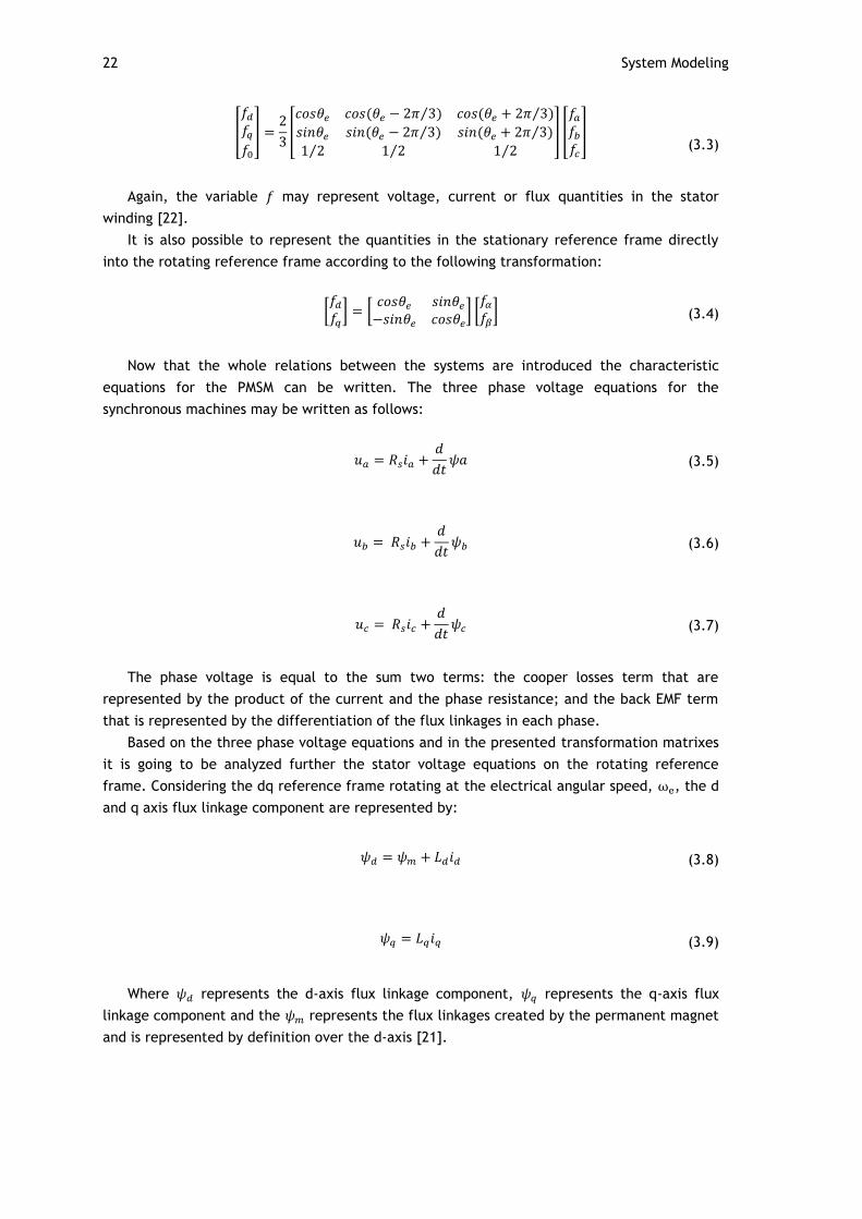
Now that the whole relations between the systems are introduced the characteristic
equations for the PMSM can be written. The three phase voltage equations for the
synchronous machines may be written as follows:
(3.5)
(3.6)
(3.7)
The phase voltage is equal to the sum two terms: the cooper losses term that are
represented by the product of the current and the phase resistance; and the back EMF term
that is represented by the differentiation of the flux linkages in each phase.
Based on the three phase voltage equations and in the presented transformation matrixes
it is going to be analyzed further the stator voltage equations on the rotating reference
frame. Considering the dq reference frame rotating at the electrical angular speed, , the d
and q axis flux linkage component are represented by:
(3.8)
(3.9)
Where represents the d-axis flux linkage component, represents the q-axis flux
linkage component and the represents the flux linkages created by the permanent magnet
and is represented by definition over the d-axis [21].

Permanent Magnet Synchronous Machines 23
The previous figure represents the simplified equivalent circuit of the PMSM in the dq
reference frame.
Where represents the resistance of the stator per phase, and represent the
inductances in the d and q axis respectively, and and represent the back EMF in the d
and q axis respectively which are produced by the d and q component of the air-gap flux
linkages. The back EMF quantities are function of speed, , of the system.
From the analysis of the equivalent circuit it is possible to write a couple of equations
according to the Kirchhoff's loop rule that represent the stator voltage equations in the dq
frame:
(3.10)
(3.11)
The previous equations result naturally in:
(3.12)
(3.13)
Replacing the flux linkages components from the equations 3.8 and 3.9 it is possible to
write a couple of equations for the stator voltages as functions of the current components in
the d and q axis [21]:
(3.14)
Figure 3.2 - Simplified equivalent circuit of the PMSM in the dq reference frame

24 System Modeling
⇒
(3.15)
For a better understanding of the behavior of the electrical quantities of the motor as in
the stator voltage and currents as well as the flux linkages, it is presented next a steady-state
vector diagram of the PMSM in dq reference frame for a given working point:
Figure 3.3 - Steady-state vector diagram of the PMSM in dq reference frame for a given working point, adapted from [21]
The vector diagram shows the amplitude and phase relations between fundamental
electrical quantities of the electric machine. The understanding of these relations is crucial
from the point of view of control, in order to find the best way to control the produced
torque.
The electromagnetic torque is by definition the cross vector product between the air-gap
flux and stator current vector apart from a gain that is proportional to the number of pole
pairs. Hence, the electromagnetic torque can be written as follows [21]:
(3.16)
The electromagnetic torque can also be calculated from the current and flux linkages in
the rotating reference frame. Thus, the electromagnetic torque can be written as [22]:
( ) (3.17)

Permanent Magnet Synchronous Machines 25
Which results in:
(3.18)
And finally the electromagnetic torque is the result of the sum of different components as
follows:
(3.19)
The first component is called excitation torque, which exists due to the influence of the
rotor flux linkage and constitutes the main component of the produced torque. The second
component is called the reluctance torque that is introduced before in this chapter. It exists
due to the rotor configuration and so it naturally depends on the saliency ratio ( ⁄ ) [22].
This component may be zero if which is the case of surface mounted PM rotors.
As matter of fact, the electromagnetic torque has another component beyond the two
specified before. This third component represents the ripple torque that appears because of
the interaction between the flux of the PM and the stator teeth. This component is difficult
to reduce and the reduction is only achieved by adopting different construction strategies.
However, the mechanical shaft coupled to the power train appears to reduce its effect.
The torque is also related with the active power of the system by means of the following
relation:
(3.20)
Where P is the active power per phase. This way for a constant torque value the power is
directly proportional to the speed.
3.1.3. Torque Angle
There are several definitions for torque angle used in the literature. For example in [2]
the torque angle is defined as the angle between the rotor flux linkage vector, which is over
the d axis, and the stator current vector. In [23] the torque angle is defined as the angle
between the terminal phase voltage and the EMF produced by the rotor permanent magnet
which is phase shifted 90º from the rotor flux linkage. In [24] the angle between the rotor flux
linkage vector and the air-gap flux linkage vector is also referred as torque angle. In this
section is going to be analyzed and clarified the use of these different angles as the torque
angle. The dependability of the produced torque as function of these angles is going to be
discussed in order to clarify the reasons of using the notion of torque angle for different
angles between different pairs of motor quantities.
The best way to understand the quantities involved in the motor operation is representing
its vectors and phases in the synchronous reference frame and analyze the relations between
them.

26 System Modeling
Hence, figure 3.4 presents a steady-state vector diagram of the PMSM in dq reference
frame for a given working point, integrating all of the relevant quantities to have in account
for the analysis.
Figure 3.4 - Steady-state vector diagram of a PMSM in dq reference frame for a given working point of motor operation
Attempting at figure 3.4, the first quantity to be analyzed is the stator current vector. Its
amplitude can be obtained from its components as follows:
√
(3.21)
The inverse of the tangent of the current components division gives the its phase angle,
:
(
) (3.22)
The current phase angle is also the angle between the rotor flux linkage and the stator
current vector and it is referred as torque angle in many scientific papers and books. As
matter of fact, it is possible to write the expression 3.18 by means of stator current
amplitude and phase just by replacing the stator current components by its trigonometric
relations:
( ) (3.23)

Permanent Magnet Synchronous Machines 27
(3.24)
Which results in:
(
)
(3.25)
From the analysis of the expression it is clear that the excitation torque component is
function of the product between rotor flux linkage, stator current and the sine of the angle
between them, which corresponds like is said before, to the phase angle, The reluctance
torque component depends just on the current amplitude and the sine of , and in case of
, this component is equal to zero. The result of this fact is the torque being directly
proportional to the sine of the current angle. From this point of view the current angle shows
a direct interference in the produced torque. Due to this reason and considering that this
angle can be directly controlled it is adopted and used as the torque angle towards the
literature.
On the other hand, the angle between the air gap flux, , which results from the
interaction between the rotor flux, , and the stator flux that is created by the stator
current, , is also referred as the torque angle. To understand its effect in the torque the
first step is writing the expression of its amplitude:
√ (3.26)
Like in the case of the stator current vector, the phase of the air gap flux, the angle that
it has with the d axis and consequently with the rotor flux linkage can be obtained from its
components as follows:
(
) (3.27)
Introducing the same analogy assumed for the stator current angle, in this case it is also
possible to write the torque expression 3.18 as function of the air gap flux amplitude and
angle, . Note that the air gap flux amplitude is function of the current components iq and
id and hence the opposite is true, it is possible to write the current components as function
of the air gap flux amplitude and phase:
(3.28)
(
)
(3.29)

28 System Modeling
Now, making the substitution of the current components as presented above in the
equation 3.18, the following expression is obtained:
( )
(
)
(3.30)
Similarly to the stator current situation, in this case the excitation torque component is
directly proportional to the product of rotor flux, air gap flux and the sine of the angle
between them. The reluctance torque component is just function of the air gap flux
amplitude and the double of the angle, being this component equal to zero in case of equal
direct and quadrature inductances. Again, the torque may be written as function of two
different quantities and the sine of the angle between them, so from this fact comes the
reason of the assumption of as the torque angle by some authors.
The last quantities missing to be analyzed are the phase, , and the EMF force, . The
stator voltage vector can also be obtained from its components in the synchronous reference
frame:
√
(3.31)
Then the stator voltage vector phase is obtained as follows:
(
) (3.32)
The EMF is the result of the rotor flux proper of the permanent magnets in the stator and
it is 90º phase shifted from the rotor flux linkage vector. Hence, the angle between stator
voltage and the EMF force is:
(3.33)
Based on this angle it is presented in [23] an expression for the electromagnetic torque as
function of the phase voltage, EMF and the angle between them. The expression is the
following:
(
)
[
( )
] (3.34)
Where is the speed of the rotor in rpm. Note that this equation depends on the speed
because the EMF is proportional to the speed. The same analogy of the angles presented
before is applied here and the excitation torque component is proportional to the sine of
and the reluctance torque component proportional to the double of like the situation for
the other presented angles, being this reluctance torque component null for the case of unity
saliency ratio. This is other approach for the notion of torque angle since an expression of

Permanent Magnet Synchronous Machines 29
torque as function of that angle is valid. From the point of view of control, this angle can be
difficult to control compared to the others.
To close this analysis the author of the present Dissertation introduces another approach
in the matter of the torque angle. Having into account that the torque vector is by definition
the cross product between two quantities as it is discussed above. The amplitude of a cross
product result corresponds to the product of the amplitude of the two quantities and the sine
of the angle between them. In other words, according to the definition of electromagnetic
torque, which depends on the cross vector product between the air-gap flux and stator
current vector, the torque angle would be defined as the angle between these two quantities.
This will lead to the following expression for the electromagnetic toque as function of the
torque angle:
(3.35)
The expression is obtained from the equation 3.16 and gives the amplitude value of the
torque being produced in a given working condition.
Hence, considering the torque angle, , from the definition of electromagnetic torque as
the angle between the stator current vector and the air gap flux linkage vector and it can be
obtained from the difference between these two vectors, hence:
(
) (
) (3.36)
It is simple to conclude that the phase of will depend directly on the phase of the
stator current vector as well as its amplitude, so for a constant value of amplitude, the air
gap flux angle will change as function of the stator current vector angle.
Considering the figure 3.4 that shows a diagram representing the quantities of a given
working point of motoring action of the machine, it is possible to conclude that the stator
current vector is leading the air gap flux vector by , in the case of generator action, the
stator current vector would be lagging the air gap flux linkage vector by which would
result in a negative value of torque. The negative sign means that the torque produced is
against the movement. In other words, the torque and torque angle have positive signs when
the torque is produced in favor of the movement which is the case of motoring action, and
negative sign in case of opposition to the movement which is the case of generator mode in
the case of regenerative braking.
It is important to understand that the different angles analyzed here that come across the
literature are not the same angle but just called the same way as consequence of the
possibility of writing a torque expression that depends on them.
All of the different approaches to the torque angle notion are thus, in the opinion of the
Author of this Dissertation, valid from the point of view of control. Hence, from the
possibility of writing an expression for the torque as function of the angular displacement
between two direct or indirect torque producing quantities, comes the notion of torque
corresponding to the angle between two vectors that have highly effect on the produced
torque. As matter of fact all of the approaches considered are used in such a way that allows
the control of the produced torque as function of direct controlled variables like the stator
current and its phase angle.

30 System Modeling
In this Dissertation, the reference to torque angle pretends to refer to the angle between
the stator current vector and the air-gap flux linkage vector according to the definition of
electromagnetic torque and it will be represented by . Although, such assumption does not
mean that the control algorithm developed will be based on the direct control of this
variable, but it will be measured and controlled by means of other quantities.
3.2. Mechanical System
The analysis of the vehicle dynamics is a complex problem and it is a relevant concern in
the domain of mechanical and fluid dynamics engineering when projecting a vehicle
propulsion system.
To simplify this analysis it is assumed that the vehicle dynamics are translated by a load
torque in the rotor shaft of the electrical motor, this way a simple expression describes the
mechanical behavior of the system in the shaft of the motor. The equation that describes the
mechanical system is represented as follows:
(3.37)
Where is the load torque, is the friction coefficient, is the moment of inertia in
and is the mechanical speed in .
The moment of inertia is related with the moment of inertia and the shaft time
constant, , by means of:
(3.38)
The shaft time constant reflects the effect of the friction and windage of the system. The
mechanical equation described in 3.37 reflects the mechanical behavior of the overall
system, and it is really important to have it into account in order to ensure the machine
synchronism.
The electromagnetic torque is the first quantity needed to be controlled so it is very
important to understand how it is produced and which variable have direct effect on the
produced torque.
3.3. PSIM Dynamic Model Simulation
In order to validate the modeling equations presented in the previous section it is
implemented in PSIM the dynamic equations of the system and then compared to the PMSM
block available in the PSIM software.
The system equations are implemented by means of a cascade of blocks connected in
order to follow the mathematical relations of the equation. The implemented sequence of
blocs is connected to an inverter driven by a regular sinusoidal PWM. In figure 3.5 is showed
the block sequence for the implementation of the motor dynamic model.

PSIM Dynamic Model Simulation 31
Figure 3.5 - PSIM Block Schematic for Dynamic Modeling of a PMSM; Mechanical Load and Inverter
As is represented in the figure, the PMSM block is connected to the same inverter of the
model in order to compare both.
It is important to notice that any control is implemented so the system is working in open
loop with no torque load. The obtained results are shown in figure 3.6.
As is shown in figure 3.6, both speed and torque are very close for both PSIM PMSM block
and implemented model which proves that the model is correctly implemented since the
results are the same for two different approaches.
Analyzing the quantities of the model, it is possible to calculate the torque angle
presented by the motor for these conditions, this way it is possible to analyze its value when
there is no presence of any kind of control.

32 System Modeling
Figure 3.6 - Speed and Torque for both model and PSIM block
Figure 3.7 - Torque and Torque Angle for a PMSM without control
Figure 3.7 shows the torque and torque angle for the motor represented by the model.
As is represented, the torque angle reaches high values in the transition state but in
steady state this value is very small for a given torque value, which means that the developed
torque may be increased by controlling the torque angle. Here enters the importance of
controlling the motor by means of torque angle in order to produce the expected torque
without consuming a high amount of current when it is possible to do it with a less amount.

Conclusion 33
3.4. Conclusion
This chapter describes the working principle of the PMSM and presents the several types
of PMSMs. It is analyzed and clarified the notion of torque angle and its relevance in the
control point of view.
The equations that model the system dynamically are presented and then a system
computational simulation based on its equations is performed.
The control methodology and how it keeps track and controls the torque angle is going to
be discussed and presented in the following chapter.

34 System Modeling

Chapter 4
System Controller Design
This chapter presents the control architecture of the developed system controller as well
as the control strategies proposed for the resolution of the proposed problem of this
Dissertation.
From the low level algorithms and strategies that control the inverter to the high level
traction control algorithm, solutions are presented, simulated and justified in order to
implement robust control architecture for the problem.
4.1. Principles of Vector Control
In scalar control, system response is low due to the coupling effect in the machine
quantities. On the other side, vector control allows the control of an AC machine as
separately excited dc motor drives.
The stator current phasor produces flux and torque. The current component producing
flux is the one in phase with the rotor flux created by the permanent magnets, oppositely the
current component producing torque is the one that is perpendicular to the rotor flux linkage
vector created by the PM [25].
The principle of vector control is decoupling the stator current into these two flux and
torque producing components and control them separately. The rotor flux linkage is, like it is
mentioned before, constant for PMSM and it constitutes the d-axis position of the dq
reference frame. Hence, the position of the rotor flux linkages at every instant is required in
vector control strategies.
Vector control strategies are classified according to how the rotor position is acquired. In
case the angle is calculated by using terminal voltages and currents, it is called as direct
vector control. In the case the angle is obtained by using rotor position measurement and
partial estimation, it is called indirect vector control [2].
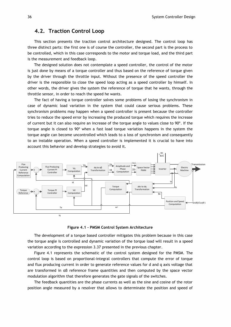
36 System Controller Design
4.2. Traction Control Loop
This section presents the traction control architecture designed. The control loop has
three distinct parts: the first one is of course the controller, the second part is the process to
be controlled, which in this case corresponds to the motor and torque load, and the third part
is the measurement and feedback loop.
The designed solution does not contemplate a speed controller, the control of the motor
is just done by means of a torque controller and thus based on the reference of torque given
by the driver through the throttle input. Without the presence of the speed controller the
driver is the responsible to close the speed loop acting as a speed controller by himself. In
other words, the driver gives the system the reference of torque that he wants, through the
throttle sensor, in order to reach the speed he wants.
The fact of having a torque controller solves some problems of losing the synchronism in
case of dynamic load variation in the system that could cause serious problems. These
synchronism problems may happen when a speed controller is present because the controller
tries to reduce the speed error by increasing the produced torque which requires the increase
of current but it can also require an increase of the torque angle to values close to 90º. If the
torque angle is closed to 90º when a fast load torque variation happens in the system the
torque angle can become uncontrolled which leads to a loss of synchronism and consequently
to an instable operation. When a speed controller is implemented it is crucial to have into
account this behavior and develop strategies to avoid it.
Electric Machine
Transmission
-+
Inverter
DCBUS
Space VectorPWM
Position and Speed Computation
Sin(θ)/Cos(θ )
abc to dqTransformation
Torque Computation
dq to αβ Transformation
Amplitude and Phase
Computation
Ia
Ib
θe
Torque PIController
Flux Producing Current PIController
VqComputation
VdComputation
Flux Producing
Current Reference
Computation
ωr
Vq
Vd
Vα
Torque Reference
Te
Iq
Vβ
|Vs|
|Vs
+-
+-
Id
Figure 4.1 - PMSM Control System Architecture
The development of a torque based controller mitigates this problem because in this case
the torque angle is controlled and dynamic variation of the torque load will result in a speed
variation according to the expression 3.37 presented in the previous chapter.
Figure 4.1 represents the schematic of the control system designed for the PMSM. The
control loop is based on proportional-integral controllers that compute the error of torque
and flux producing current in order to generate reference values for d and q axis voltage that
are transformed in αβ reference frame quantities and then computed by the space vector
modulation algorithm that therefore generates the gate signals of the switches.
The feedback quantities are the phase currents as well as the sine and cosine of the rotor
position angle measured by a resolver that allows to determinate the position and speed of

Traction Control Loop 37
the rotor as it will be explained further. Only two of the three phase currents are needed to
be measured and the third one can be obtained from the other two.
The transformation blocks represented in the schematic are explained in the previous
chapter. The Torque Computation block uses the equation 3.18 to calculate the torque from
the values of iq and id. The Space Vector PWM block generates the gate signals from the
values of amplitude and phase of the phase voltage and it will be explained further in this
chapter as well as the Position and Speed Computation block. The Flux Producing Current
Reference Computation block is the block responsible to implement the method of control.
The content of this block may change in order to implement different control strategies. The
next section introduces and explains the main strategies developed for the control
architecture from the torque producing current generation till the flux producing current
reference generation.
4.3. Traction Control Methods
This section explains the control algorithms developed for the generation of the control
references for iq and id. The generation of the q axis current is inherent to the torque
reference which is an input of the system, coming from the throttle and brake pedal. On the
other hand the reference of the id will depend on the control method implemented in order
to control different variables in different ways to find the best control method for torque
production in each situation.
It is presented next different algorithms for generation of the d axis current allowing the
implementation of different control strategies.
4.3.1. Current Angle Based Torque Control
This control method for id reference generation directly controls the value of id and it
depends naturally on the effect of each component of the stator current in the torque
produced.
Analyzing the torque equation 3.18 presented in the chapter before:
(4.1)
From what is discussed in the previous chapter, the expression of the torque as function
of the amplitude may be obtained by replacing id and iq in the previous expression,
resulting in the expression 4.2:
( ( )
( )
) (4.2)
A simplification of the expression is obtained if its second component is eliminated by
giving an id reference equal to zero which results in a reluctance torque component equal to
zero as it is introduced in the previous chapter. The objective of this method is to give a

38 System Controller Design
reference of d axis current equal to zero, which will lead to a torque expression only
dependable on the iq value and consequently directly proportional to the amplitude of the
phase current.
To clarify this control method it is important to start analyzing the current vector, the
value of the d axis current being equal to zero has the following implications:
⇒ (
) ⇒ (4.3)
Now, replacing the conditions in the previous equations it is obtained:
(4.4)
Or as function of :
(
) ⇒
(4.5)
Hence, the torque can be directly controlled proportionally to the value of the amplitude
of the phase current and in these conditions the torque has its maximum value because
and the sine function has its maximum value for this angle.
Figure 4.2 shows the computational simulation for this control considering a torque
reference of 10 Nm. The stator phase currents as well as the current angle response and
torque response are represented.
Figure 4.2 - Torque response; Stator phase currents and current angle for the Current Based Angle Torque Control
As is represented, the start-up is really smooth since the id component is kept at zero the
stator current amplitude is equal to iq which increases proportional to the torque. Note that
there is no overshoot of the torque response for the tuned PI controller gains. As matter of
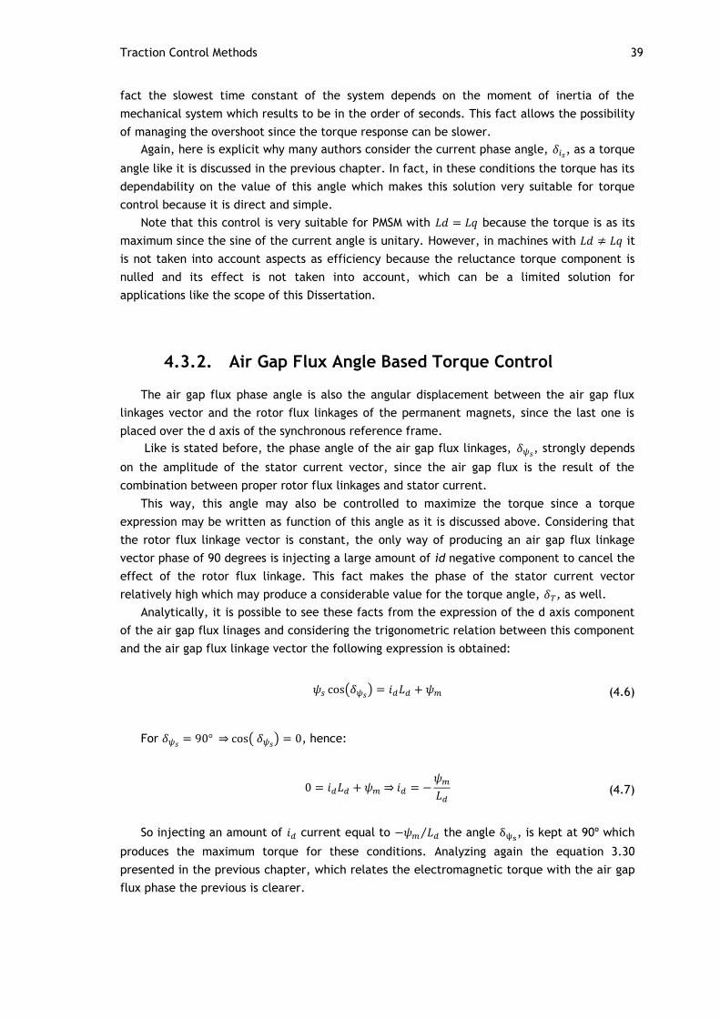
Traction Control Methods 39
fact the slowest time constant of the system depends on the moment of inertia of the
mechanical system which results to be in the order of seconds. This fact allows the possibility
of managing the overshoot since the torque response can be slower.
Again, here is explicit why many authors consider the current phase angle, , as a torque
angle like it is discussed in the previous chapter. In fact, in these conditions the torque has its
dependability on the value of this angle which makes this solution very suitable for torque
control because it is direct and simple.
Note that this control is very suitable for PMSM with because the torque is as its
maximum since the sine of the current angle is unitary. However, in machines with it
is not taken into account aspects as efficiency because the reluctance torque component is
nulled and its effect is not taken into account, which can be a limited solution for
applications like the scope of this Dissertation.
4.3.2. Air Gap Flux Angle Based Torque Control
The air gap flux phase angle is also the angular displacement between the air gap flux
linkages vector and the rotor flux linkages of the permanent magnets, since the last one is
placed over the d axis of the synchronous reference frame.
Like is stated before, the phase angle of the air gap flux linkages, , strongly depends
on the amplitude of the stator current vector, since the air gap flux is the result of the
combination between proper rotor flux linkages and stator current.
This way, this angle may also be controlled to maximize the torque since a torque
expression may be written as function of this angle as it is discussed above. Considering that
the rotor flux linkage vector is constant, the only way of producing an air gap flux linkage
vector phase of 90 degrees is injecting a large amount of id negative component to cancel the
effect of the rotor flux linkage. This fact makes the phase of the stator current vector
relatively high which may produce a considerable value for the torque angle, , as well.
Analytically, it is possible to see these facts from the expression of the d axis component
of the air gap flux linages and considering the trigonometric relation between this component
and the air gap flux linkage vector the following expression is obtained:
( ) (4.6)
For ⇒ (
) , hence:
⇒
(4.7)
So injecting an amount of current equal to ⁄ the angle , is kept at 90º which
produces the maximum torque for these conditions. Analyzing again the equation 3.30
presented in the previous chapter, which relates the electromagnetic torque with the air gap
flux phase the previous is clearer.

40 System Controller Design
Figure 4.3 shows the computational simulation results for this control in the exact
conditions of the other cases. Again, the torque and air gap flux phase response are
represented as well as the three phase stator currents.
Figure 4.3 - Torque response; Stator phase currents and current angle for the Air Gap Flux Based Angle Torque Control
Although the simulation is carried out under the same conditions of the Current Angle
Based Torque Control note that here a small overshoot is present in the torque response. This
happens because the start-up current is also much higher than in the case of the Current
Angle Based Torque Control which is a consequence of the constant reference of id that is
needed to null the effect of the rotor flux linkages right from the beginning.
Comparing with the Current Angle Based Torque Control this one has in fact a higher
start-up current but on the other hand it results to absolve slightly less current in steady state
in the same conditions. Actually the amplitude of the phase currents in steady state appears
to be 12% to 15% less than when the current angle is controlled to 90 degrees.
As matter of fact, the problem of the high start-up current may be overcome by
generating an internal ramp reference for the id current. To illustrate this solution it is
presented in figure 4.4 the simulating results for the same previous conditions but with an
internal ramp reference for the id component.

Traction Control Methods 41
Figure 4.4 - Torque response; Stator phase currents and current angle for the Air Gap Flux Based Angle Torque Control with an id ramp reference
As is represented, introducing an id component ramp reference in the beginning the
absorbed current is considerably reduced. Note that the overshoot is higher than with the
constant id reference although it is possible to reduce it by changing resynchronize the PI
gains. With this improvement this control method shows a very interesting response,
producing the same value of torque as the Current Angle Based Torque Control but requiring
less current.
Regarding of its effect on the produced torque it is reasonable that some authors consider
this angle the torque angle like it is said before, this way the produced torque is maximized
as function of the angle between the rotor flux and the air gap flux linkages for each working
condition. This approach is simple because the value of id is constant for all working points
since the value of the rotor flux linkages is constant, the drawback of this control is the start-
up, a large amount of d axis component of current is needed since the reference is generated
right from the start-up which results in a high current step at the start-up.
In the case of unitary saliency ration PMSM this control may not be so interesting because
the torque expression does not depend directly on the stator current. This fact means that
the torque is not controlled as function of the current vector and thus controlling the angle
to be 90 degrees may require an incredible high value of stator current.
4.3.3. Direct Torque Angle control
Another approach to generate an id reference is developed based on the direct control of
the torque angle, , analyzing the equation presented in the previous chapter:
(4.8)
It is simple to conclude that in the matter of the torque angle value, the torque has its
maximum value for torque angle of 90º which is the positive angle of which the sine is
unitary. So the aim of the developed control is to generate a reference value of id that
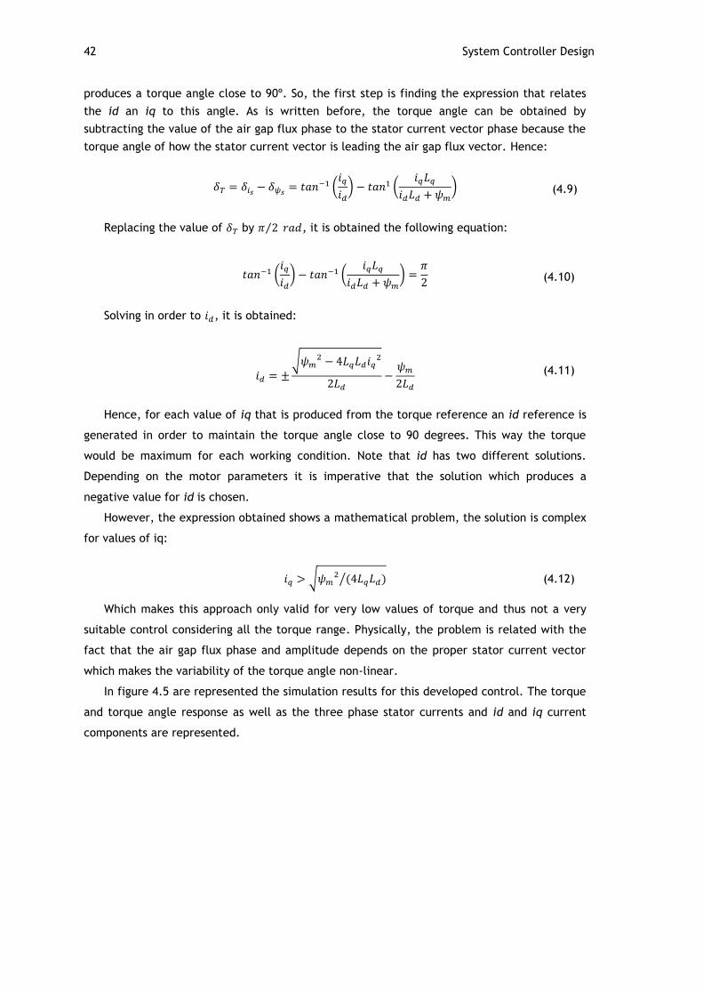
42 System Controller Design
produces a torque angle close to 90º. So, the first step is finding the expression that relates
the id an iq to this angle. As is written before, the torque angle can be obtained by
subtracting the value of the air gap flux phase to the stator current vector phase because the
torque angle of how the stator current vector is leading the air gap flux vector. Hence:
(
) (
) (4.9)
Replacing the value of by ⁄ , it is obtained the following equation:
(
) (
)
(4.10)
Solving in order to , it is obtained:
√
(4.11)
Hence, for each value of iq that is produced from the torque reference an id reference is
generated in order to maintain the torque angle close to 90 degrees. This way the torque
would be maximum for each working condition. Note that id has two different solutions.
Depending on the motor parameters it is imperative that the solution which produces a
negative value for id is chosen.
However, the expression obtained shows a mathematical problem, the solution is complex
for values of iq:
√ ⁄ (4.12)
Which makes this approach only valid for very low values of torque and thus not a very
suitable control considering all the torque range. Physically, the problem is related with the
fact that the air gap flux phase and amplitude depends on the proper stator current vector
which makes the variability of the torque angle non-linear.
In figure 4.5 are represented the simulation results for this developed control. The torque
and torque angle response as well as the three phase stator currents and id and iq current
components are represented.

Traction Control Methods 43
Figure 4.5 - Torque response; Stator phase currents and current angle for the Direct Torque Angle Control
Note in first place that this time the torque reference is not 10 Nm but just 4 Nm. This is
because as is introduced above this control is just applicable for a given range of iq
component value. In this case, for the motor model used in this simulation the maximum
value that this control allows is around 4 Nm and thus the reference is established in that
value.
Analyzing the current components it is possible to conclude that the id component have a
really high negative value which means that the field is weakened. The start-up current is
very high in comparison to the Current Angle Based Torque Control and really close to the
case of the Air Gap Flux Angle Based Torque Control. Actually the value of the air gap flux
results to be over 80 degrees which means it is almost 90 degrees so the effect is almost the
same considering the current phase is also very high resulting in an id component almost as
high as the rotor flux linkages produced by the permanent magnets. Hence, regarding of the
current absorption this control is not very interesting, not just because it is only applicable
for a low value of torque but also because it requires almost as much current as the previous
control to produce less than half of the torque being produced in the conditions of the
previous control simulation. So this control is not very suitable for controlling PMSM with
.
On the other hand, note that in case of PMSM with this control results to be very
close the Current Angle Based Torque Control since both of the torque expressions results to
be function of the stator current.

44 System Controller Design
4.3.4. Maximum Torque Per Ampere Control
Considering that for applications like electric or hybrid electric vehicles the efficiency and
performance is a relevant matter to have in account. As is discussed previously depending on
the control method implemented, the same torque value may be obtained for different
amplitudes of phase currents. Hence, it is reasonable and expectable to have a control
method that takes that into account.
Taking this consideration, it is developed a control algorithm that generates a d axis
current component which produces minimum current absorption for a given torque. There is a
torque/current ratio that when maximized allows a maximum torque per ampere control.
Note that in case of equal d and q axis inductance motors the previous is achieved in a very
direct way since the torque expression only has a component. However, in the case of motors
with saliency ratio different than one a deeper analysis is needed since the torque results to
be a sum of different components.
Hence, an expression for the torque/current ratio is obtained starting from the equation
3.18 presented in the previous chapter.
Replacing the current d and q components it is obtained a torque expression as a function
of the stator current and the current phase, , which results to be the equation number
3.25 of the previous chapter:
Then the torque/current ratio is obtained:
( )
(4.13)
Now, differentiating in order to the torque/current ratio the following expression is
obtained:
(
)
( ) (4.14)
The last step is to replace the current angle functions by d and q current components and
find the values of id where the differentiation of the function is zero which corresponds to
the maximum or minimum of the equation of the ratio.
Hence, solving the following equation:
( ( ) ( ) ( )) ⇔
⇔ ( )(
) (4.15)
It is obtained an expression for id as function as iq that produces an optimum working
point with a minimum current for a given torque. The expression is presented above:
( ) √
(4.16)

Traction Control Methods 45
The implementation of the previous equation generates the d axis component current as
function of the q axis component value that is produced as function of the torque reference.
Note that the equation 4.16 has more than one solution, but the solution chosen is the one
that keeps the id with a negative value in order to generate a flux in opposition to the one
created by the magnet.
In figure 4.6 is represented the computational simulation results for the developed
control. The torque response as well as stator current angle and air gap flux angle are
represented. Again the three phase stator currents and the id and iq current components are
also represented for further analysis.
Figure 4.6 - Torque response; Stator phase currents and current angle for the Maximum Torque per Ampere Control
As expected this control is far way the best regarding the amount of current needed for
the developed torque. As matter of fact, for the same conditions of the other simulations this
control allows an achievement of 36% reduction in the stator amplitude current needed.
Analyzing the air gap flux phase is it shown that this control keeps it with a high value
over 70 degrees and note that the start-up is really smooth because the air gap flux phase is
slowly increased. This fact is the result of the control generating a id reference that reduces
the instantaneous amount of current per torque unit.
On the other hand the phase current is kept high, over 90º which results in a negative id
component suggesting a field weakening operation. As matter of fact it is weakening the field
that it is possible to obtain low values of stator current per unit of torque.
This control approach for id reference generation is the one with the best results in what
matters to produced torque as function of phase current absorption in PMSM with .
This fact makes this control method very suitable for this kind of application when PMSM with
saliency ratio different then the unity.

46 System Controller Design
4.3.5. Regenerative Braking
Like it is introduced before, the regenerative braking is the action of braking the vehicle
electrically and use the produced energy to charge the batteries or the super capacitors.
Basically, it transforms the kinetic energy into electrical energy using the motor as electrical
generator and sends the energy back to the system. This action of producing the electric
energy from the mechanical energy creates a torque in opposition to the movement that
slows down the speed braking the vehicle.
This operation is very similar to the motor operation the only difference here is that the
stator current vector is lagging the air gap flux vector contrarily to what happens in the motor
operation. Hence, the torque angle is negative for generator operation.
In figure 4.7, it is represented a steady-state vector diagram of a given working point in
generator operation. As it is shown the stator current vector is now in the third quadrant
lagging the air gap flux vector by .
Figure 4.7 - Steady-state vector diagram of a PMSM in dq reference frame for a given working point of generator operation
From the controller point of view the generator operation can be obtained making the
torque angle negative which can be obtained introducing a negative reference of torque that
will produce a negative reference of torque producing current and consequently a current
vector that will lag the air gap flux vector.
Figure 4.8 represents the computational simulation for regenerative braking operation.
The torque response as well as phase currents, speed and instantaneous power are displaced
in figure 4.8 for further analysis.

Traction Control Methods 47
Figure 4.8 - Regenerative Braking operation
In first place a positive torque of 10 Nm reference is given to the controller and the motor
stars up and accelerates increasing the speed. At t=0.3s the reference is changed to -5 Nm
simulating a braking request. When the torque starts to have a negative value the speed does
not decrease immediately due to the system inertia but after a small amount of time the
speed starts decreasing and the average power measured at the source terminals changes its
signal signalizing the change in the direction of the power flow. The motor is working as a
generator and producing energy to the energy storage system.
Figure 4.9 - Stator current phase, air gap flux phase and stator voltage phase for motoring and regenerative operation
To illustrate the operation of the motor as generator it is presented in figure 4.9 the
stator current phase, air gap flux phase and stator voltage phase for the conditions of figure
4.8.

48 System Controller Design
Note that until t=0.36s the electric machine is working as a motor and thus the quantities
respective phases are in agreement with the conditions presented in figure 3.4. On the hand,
after t=3.6s the electric machine starts working as a generator, and now the stator current
vector is lagging the air gap flux vector and the stator voltage vector is in phase opposition to
the stator current vector agreeing with the diagram of figure 4.7.
The regenerative braking is a good resource to improve the overall energetic balance of
the vehicle system. Although it has some implications at the hardware level, the inverter and
the switches drivers must be perfectly adapted for energy recovery. Furthermore it is also
imperative the availability of a mechanical brake in the vehicle to ensure the security of the
vehicle.
4.3.6. Start-Up
Using an inductive sensor like a resolver has the problem of starting up the motor because
the resolver does not generate the output signal while the speed does not reach a minimum
value. Hence, at the start-up point the controller is not able to know the position of the rotor
and so it is impossible to synchronize the rotating reference frame with the rotor. This way a
solution is needed to put the motor running in open loop and then close the loop when the
position signal from the resolver is available.
The developed solution for the electric motor start-up intends to feed gradually the motor
with an increasing current producing an increasing torque which will make the rotor move and
once the signal of the position is available this information is fed back into the controller and
the synchronization is done after a small transitory amount of time. This is done by reading
the reference of torque from the throttle sensor and giving it to the controller an incremental
reference to guaranty a smooth star up as possible. While there is no signal from the resolver
the rotor position is considered to be zero and the controller will continue to increase the
current injected until the resolver gives a measurable signal. Therefore, the controller is fed
back with actual absolute rotor position and instantaneous speed and the synchronization is
done.
4.4. PI Controllers
PI controllers may not provide optimal control in some applications but they are linear
and simple to implement and widely used in similar applications. Hence, the PI controller is
considered for the development of this system.
There are two PI controllers in the control loop, one is responsible of computing the
torque error and the other one is responsible of computing the error of id current component.
Considering the PI standard form it is described as follows:
(
∫
) (4.17)
Where is the error, is the proportional gain, and is the integral time. The
integrative gain results to be ⁄ .

PI Controllers 49
The standard form is also used in the PSIM PI block. This form facilitates the manual gain
tuning because there is just one gain to tune which is the proportional gain and afterwards it
is finally adjusted the integration time.
The PI output is used to calculate the stator voltages components d and q. The torque PI
output is summed to the speed and id dependent components to generate Vq. On the other
side, the Vd component is calculated summing the id PI output to the iq and speed dependent
terms.
The Vq and Vd components are highly coupled and this fact does not make the PI tuning a
simple task. The PI tuning is done with help in the PSIM computational simulations. In first
place the proportional gain is adjusted observing the system output having into account the
rise time as well as the overshoot and mainly the stability of the system, keeping the
proportional gain as small as possible. Therefore it is adjusted the integral time in order to
eliminate the steady state error having into account the stability of the system.
4.5. Space Vector PWM
The space vector pulse with modulation is a technique used to generate the gate signals
for the 6 switches of the inverter. This section explains the functionality of the Space Vector
PWM block as well as the Amplitude and Phase Computation block.
Basically, the Amplitude and Phase Computation block calculates the phase, , and
amplitude, , of the phase voltage from its components in the stationary reference frame
as follows:
√
(4.18)
(
) (4.19)
Considering the implementation of a sinusoidal PWM technique the amplitude and phase
of the stator voltage in the stationary reference frame are then transformed again in three
phase quantities that are then compared with a triangular carrier wave to generate the gate
signals. The sinusoidal PWM is a very simple technique although it has some drawbacks like
the need of high switching frequency that result in switching losses and mainly the relatively
small line range which results in a reduction of the available voltage. Over modulation may
also occur which generates more sideband harmonics.
To overcome the sinusoidal PWM issues, a space vector PWM technique is implemented.
Contrarily to the sinusoidal PWM technique, the Space Vector PWM block computes the stator
voltage amplitude and phase quantities in order to produce the stator voltage vector by
combination of the inverter state vectors. Each vector is referred to an on/off combination of
the three top inverter switches. Table 4.1 shows the inverter on/off combinations of each
state vector.

50 System Controller Design
Table 4.1 – Three Phase Inverter Switching Vector States
Vector Value
0 0 0 0
1 0 0
1 1 0
0 1 0
0 1 1
0 0 1
1 0 1
1 1 1 0
Hence, the Space Vector technique synthetizes the voltage reference obtained from the
αβ reference frame components, using a combination of two adjacent switching vectors and
the zero vector. There are 8 switching vectors of which 2 are zero vectors and the other 6
correspond to the combinations of on/off states that are possible to happen amongst the
three top transistors as is represented in table 4.1.
The first step is to determinate the sector where the stator voltage is located and the
angle that the voltage vector have inside of that sector. This can be done by analyzing the
value of the voltage phase. First finding the sector, and afterwards, the angle that the vector
have inside of the sector that is going to be called can be obtained as follows:
(4.20)
Where corresponds to the number of the sector. Since there are 6 sectors each one
occupies 60º of the reference frame as it is represented in figure 4.10. Hence, computing the
difference between and 60 times the number of sectors minus the one where the vector is
located, the value of is obtained.

Space Vector PWM 51
Figure 4.10 - Space vectors of a three-phase bridge inverter (adapted from [26])
The next step is computing the times for the application of each boundary vector. It is
needed to compute the time for the lower boundary vector of the sector, , the time of the
higher boundary vector of the sector, , and finally the time for the application of the
vector zero, . Naturally, these times have to be generated over a modulation signal of
frequency equal to ⁄ in order to produce a time average equal to the sampled value of
the reference vector. Hence, the reference stator voltage vector may be obtained as function
the modulation times as follows:
(4.21)
Where:
(4.22)
The duty cycles for each vector are equal to ⁄ , ⁄ and ⁄ respectively. Using
trigonometric relations between the angles and the sector limit vectors it is found the
expression for the vectors and :
| |
| | [
√ ] (4.23)
| |
| | [
√ ] (4.24)

52 System Controller Design
Now it is finally possible to compute the times as:
| | [
√ ] (4.25)
| | [
√ ] (4.26)
(4.27)
The time , is obtained by subtracting the nonzero vector times to the period , and
this equations are valid for all sectors by replacing the indents by the respective number of
the sector [27]. Note that the times here are being calculated considering a star connection.
In case of delta connection a factor of √ has to be considered in the voltage value of the DC
link.
The next stage of the algorithm is to generate a switching sequence with the expected
duty cycles for each vector in a center-weighted PWM sequence over the period . To
achieve this, it is developed a solution based on a triangular wave with period , amplitude
and duty cycle of 0.5. The idea is to compare the time values with the amplitude of the
triangular wave in order to generate a pulse with the width necessary to implement the
expected sequence.
The sequence implemented requires 3 vectors in 5 transitions where the beginning and
the end of the sequence correspond to half of the time of the vector zero. Then, between the
vector zero and the vector in the center it is half of the time of the vector for an even
sector. In the case of an odd sector, the sequence has half of the time of the vector before
and after the time of the vector that is now in the center. Note that this technique only
requires three different vectors in 5 transitions because only one of the zero vectors is used
this way the number of commutations is reduced and consequently there are less switching
losses. The only vector with zero voltage value used is the vector presented in table 4.1,
this vector corresponds to the switching combination where the three top transistors are not
conducting. The use of the zero voltage vector where the three top transistors are in
conduction is not a healthy solution when using permanent magnet synchronous machines.
Finally, the final sequence will have different intermediate times which depend on
whether the sector is odd or even and thus the sequence times will be called hereafter:
, for the vector located in the center of the sequence and , for the vector around
it. These times are obtained from and as follows:
{
} (4.28)

Space Vector PWM 53
{
} (4.29)
The difference between even and odd vectors is just a swop in which boundary vector is
generated first, this fact is just to keep the center waited pulse sequence.
The sequence is generated comparing the reference time values with the triangular wave,
resulting in true when the wave is higher than the reference values and false when it is not.
To better understand the process described above it is represented in figure 4.11 an
illustration of all the steps of the technique that generates the pulses.
Figure 4.11 - Sequence timing generation stages
The result from the comparisons when summed result in a signal with three step values.
Each step has the expected width for the vector. The three step values 1, 2 and 3 correspond
to the vectors , and respectively. This technique facilitates the process because this
signal together with the number of the sector are then used as inputs of a lookup table that
does the selection of the respective switching vectors and converts it in the gating signal with
pulses with the width equal to the width of the correspondent step.
Each switch has to have a lookup table with the correspondent states of the respective
switch in order to turn it on or off as function of the sector number and the boundary vector
selector signal. The lookup tables of the bottom switches are the inverse of the respective
top leg switch.
To illustrate the functionality of the lookup tables it is represented in the table 4.2 the
lookup tables content for the three top switches of the inverter as function of the inputs
sector and boundary vector selector signal.

54 System Controller Design
Table 4.2 - Lookup Tables for the three top inverter switches
(1)
(2)
(3)
(1)
(2)
(3)
(1)
(2)
(3)
Sector 1 0 1 1 Sector 1 0 0 1 Sector 1 0 0 0
Sector 2 0 0 1 Sector 2 0 1 1 Sector 2 0 0 0
Sector 3 0 0 0 Sector 3 0 1 1 Sector 3 0 0 1
Sector 4 0 0 0 Sector 4 0 0 1 Sector 4 0 1 1
Sector 5 0 0 1 Sector 5 0 0 0 Sector 5 0 1 1
Sector 6 0 1 1 Sector 6 0 0 0 Sector 6 0 0 1
The Space Vector PWM algorithm described above is implemented in the PSIM software
with a carrier frequency of with result in a of 100 . The figure 4.12 shows the
developed block sequence for the implementation of the SVPWM algorithm.
Figure 4.12 - PSIM block schematic for the Space Vector PWM algorithm
The Space Vector modulation technique together with the developed control allows the
generation of the phase voltages with a modulated sinusoidal shape as is visible in figure 4.13.
Figure 4.13 - Phase voltages of phase a, b and c

Space Vector PWM 55
The Space Vector modulation technique is very suited for three phase electric machine
control because the space vectors describe the machine in both steady and transient state
operation and besides this technique generates low THD, the unexpected low order harmonics
are reduced.
4.6. Rotor position and Speed Computation
This section states an important part of the control loop. Like it is previously said in this
report the vectorial control strategies for electrical machines require that the controller has
the information about the position of the rotor. Thus it is needed to measure or to
determinate the position of the rotor. It will be presented next the two ways of obtaining this
information, the first one is the sensorless solution and the second one requires physical
sensors to measure the rotor position. Basically, it is going to be presented here the
functionality of the Position and Speed Computation block represented in figure 4.1.
4.6.1. Sensorless Estimation
Control methods based on sensorless estimation techniques are normally called direct
methods of obtaining the position because it does not use any kind of sensors beyond the ones
that are necessary to measure the stator phase currents and stator phase voltages. These
methods are based on software computation based on the motor parameters and can be
implemented according to different techniques.
The most used techniques are: Back-EMF estimators; State observers; Sliding-mode
observers; High-frequency signal injection and PLL-based estimators.
The Back-EMF estimators require the measurement of phase currents and voltages in
order to obtain the air-gap flux vector module and phase in the stationary reference frame.
The rotor position is considered to be given by the angle of stator flux. This technique has
some accuracy issues because it is considered that speed variations are null and besides at
low frequencies the accusation of stator phase voltages is difficult.
The second technique is the state observer technique which is a closed-loop estimator.
This technique estimates the rotor position by means of motor parameters variations as in
inductance variations due to saturation of the magnetic circuits. There are several kinds of
state observers sensorless controls but all of them always reveal inaccuracies because a very
detailed dynamic model of the PMSM is needed and most of the times dynamic models do not
consider parameter variations due to temperature effect.
The sliding-mode observer is another sensorless technique for rotor position estimation.
This technique is based on the motor state variables. Basically, a limited surface is defined
like a hysteresis window. The control signal forces the system to slide along the surface
within its limits. Again, this technique requires the measurement of the phase stator currents
which means that high filter properties are needed. The sliding-mode observer is considered
one of the most robust and less sensible to parameter variations among the presented
techniques.

56 System Controller Design
The high-frequency signal injection is, like the name suggests, a technique where a high
frequency voltage signal is injected in one of the three phases. Afterwards, the current is
measured in order to detect the position of the d-axis. The current measured will be
dependent on the inductance, in other words the current will have its highest value for the
lowest value of inductance which corresponds to the position of the d-axis. Note that this
technique is only valid for motors where the saliency ration is not unitary. The main problem
of this approach is the necessity of high speed measurements as well as high precision and
high processing ability. The occurrence of torque ripple, vibrations and audible noises can be
also a consequence of this technique.
The last technique is the PLL-based estimator. In this case the rotor position and speed
are estimated by estimating a dq reference frame and then synchronize it with the real rotor
dq reference frame. The objective is to estimate the back-EMF produced by the permanent
magnet and then null its d-axis component in the estimated reference frame. When the d-axis
component of the back-EMF is zero in the estimated reference frame the back-EMF
component is over the q-axis which is its natural position since the back-EMF is 90º phase
shifted from the rotor flux linkages vector that is placed over the d-axis.
The PLL technique uses PI controllers to eliminate the error between the estimated frame
and the real one synchronizing them. This technique is very robust however it has some
inaccuracies at low speed because the back-EMF is proportional to the speed and hence it
requires a minimum value of speed in order to have a measurable value.
A more detailed description about sensorless control strategies can be found in [28]. The
sensorless control may be a good solution but although its advantages, like the non-necessity
of using physical sensors this technique is quite complex from the point of view of
implementation and also from the point of view of computing capability due to the amount of
complex real time calculations it requires. Because of these reasons it is common the
measurement of the rotor position by means of physical sensors attached to the rotor of the
motor.
4.6.2. Sensor Acquisition
Contrarily to sensorless based controls, control methods that measure the rotor position
angle are normally called indirect methods. The information about position and consequently
speed are acquired by means of physical sensors like an encoder or a resolver.
An encoder is an electromagnetic device that counts or reproduces electric pulses from a
rotational movement of its axis. On the other side, a resolver is a device similar to a small
motor: it has a stator and a rotor. The rotor is mechanically coupled to the rotor of the motor
and it has a coil, which is the secondary winding of the turning transformer, and a separate
primary winding in a lamination, it excites two phase windings that are placed in the stator
and configured 90º from each other, one of the windings produces a sine output and the other
one a cosine output that correspond to the sine and cosine of the angle that corresponds to
the position of its rotor.
Note that the number of poles of the motor and the number of poles of the resolver have
to be considered. If the motor and the resolver have the same number of poles then the
position information given by the resolver corresponds to the position of the motor’s rotor.
However, if the resolver does not have the same number of poles of the motor then a
multiplicative factor has to be taken into account.

Rotor Position and Speed Computation 57
Hence, dividing the resolver’s sine signal by the cosine signal, the tangent of the
resolver’s position is obtained. Therefore, the absolute rotor position may be obtained as
follows:
⇒ (
) (4.30)
Where is the multiplicative factor that depends on the number of poles of the
resolver and the motor. is then given by the ratio between the number of the motor
poles and resolver poles as follows:
(4.31)
Where is the number of motor poles and is the number of resolver poles. As it is
introduced above, results to be one in case the number of poles are equal.
The control system developed in this Dissertation is based on position acquisition by
means of a resolver and thus the resolver PSIM block is used to measure and feeds back the
information of the position of the rotor to the control system.
The output of the resolver is a sine and a cosine signal that is computed and the angle is
obtained by means of the equation 4.30.
Afterwards, based on the information of the position, the speed has to be calculated it is
thus implemented a discrete derivative of the position. Hence, the speed is calculated as
follows:
(4.32)
Where the is the derivative time constant and is the last value of the rotor
position stored seconds before.
For computational simulation purposes the position and speed computation described
above is implemented in C language using a PSIM C Block. Figure 4.14 shows the schematic of
this implementation in PSIM.

58 System Controller Design
Figure 4.14 - Position and Speed Computation Block implemented in PSIM (left) and the respective speed and position signals for motoring operation (right)
The rotor electrical position, , and the rotor electrical speed, , information are then
fed back into the control.
The calculations done in this case are far way less complex than when a sensorless
computation is implemented and so the controller design is simpler.
4.7. PSIM Torque Control System Simulation
This section pretends to state and discuss the computational results obtained for the
overall torque control algorithm developed and implemented in the PSIM software. Here the
simulation is already carried out considering the parameters of the motor that would be used
in the prototype in order to obtain results as close as possible to the real ones.
The motor considered for the implementation is the PERM 156. The first particularity to
attempt to is the topology of the motor. This motor is a pancake type of PMSM which is a
recent technology in this field which allows it to be a very compact motor with a surface
mounted PM rotor and consequently for the reasons explained previously in this
Dissertation.
This motor will be more detailed described in the following chapter. Here is only needed
to specify the electrical characteristics described in table 4.3 which presents the needed
characteristics for the computational simulation:
Table 4.3 - Relevant parameters for the control simulation of the PERM 156 PM motor
Motor Parameters
Rs: 1.7 mΩ
Ls=Ld=Lq: 15.8 μH
Moment of Inertia: 0.00586
Vk/krpm: 8.87
Pole Pairs: 4

PSIM Torque Control System Simulation 59
Figure 4.15 shows the overall simulating system developed in PSIM.
Figure 4.15 - Control and power system implemented in PSIM
The power system is implemented as well and then the inverter and the electric motor
are connected to a mechanical load and then the several parts of the control loop described
before are integrated to close the loop and control the system.
Considering the type of the motor, three of the developed controls described previously in
this chapter are implemented and simulated for this motor. The MTPA control it is not
applicable in this case since the motor has saliency ratio equal to one. Hence, just the
Current Angle Based Torque Control; the Air Gap Flux Angle Based Torque Control and the
Direct Torque Angle Control are implemented and simulated.
Figure 4.16 shows the computational simulation results for Air Gap Flux Angle Based
Torque Control.

60 System Controller Design
Figure 4.16 - PERM 156 Air Gap Flux Angle Based Torque Control
For a torque reference of 20 Nm is it represented in figure 4.16 the relevant quantities for
this control method. The torque response is really fast. As is shown, the id component has a
really high value due to the low value of the stator inductance. This fact results in a high
value of stator current amplitude required to make the delta_phi angle equal to 90 degrees.
This control when applied to motors with equal direct and quadrature inductances is not
interesting from a point of view of current consumption which means that regarding of
motoring action this method is not a solution if less current consumption for the same value
of torque is achieved by means of other strategies.
Figure 4.17 presents the computational simulation results for Direct Torque Angle Control.
Figure 4.17 - PERM 156 Direct Torque Angle Control
From the analysis of the figure is possible to conclude that in comparison to the Air Gap
Flux Angle Based Torque Control this one is much better regarding of the current

PSIM Torque Control System Simulation 61
consumption for the same value of torque. It is achieved a current reduction of around 64 %
comparing to the previous control method.
This control is a good solution concerning the torque/current ratio but it has the problem
described in section 4.3.3 and thus the control is just applicable for id component values up
to 386 A as described in equation 4.12.
Figure 4.18 computational simulation results for the Current Angle Based Torque Control.
Figure 4.18 - PERM 156 Current Angle Based Torque Control
As is discussed before the Current Angle Based Control results to be very similar to the
Direct Torque Angle Control. As matter of fact regarding the torque/current ration, this
control presents very good results. Comparing to the Direct Torque Angle Control, this
method presents around 8 % less of current amplitude for the same developed torque. Besides
that, this control may also be used for the entire range of iq component values which makes
this control very suitable for the control of the PERM 156 for this application.
4.8. High Level Control Algorithm
In this section is presented the high level control algorithm of the electric traction system
unit for the vehicle. It is at this level that the communication between the other control
system units happen mainly the important information from the Energy Management Control
Unit about the state of charge. Based on this information the control algorithm decides
whether is possible or not to do regenerative braking, and if it is possible to run at full power
or if is necessary to limit it in order to extend the battery charge to finish a programed trip.
Figure 4.19 shows a schematic of the state machine developed for the high level control
algorithm developed.

62 System Controller Design
((Brake > Security Boundary)or
(SOC = Full))
Power Up(Rest)
Key Key
Start-Up Forward(Open Loop)
((Throttle and Forward) and (not Brake)) Start-Up Reverse(Open Loop)
((Throttle and Reverse) and (not brake))
Forward(Closed Loop)
Resolver Signal
Reverse(Closed Loop)
Resolver Signal
Smooth Energy Recovery
not Throttle
Throttle
Progressive Regenerative
Braking
Brake
(Throttle and (not Brake))
Brake
Idle(Position Stored)
Speed = 0
Speed = 0
Brake
((Throttle and Forward) and (not Brake))
Mechanical Brake
Brake
Speed = 0
((Throttle and Reverse) and (not brake))
Brake
Error
Power off
not Key
not Key
((Throttle and Reverse) And
(not brake))
((Throttle and Forward) and
(not Brake))
Figure 4.19 - High level algorithm
It is during the Reverse; Forward; Smooth Energy Recovery and the Progressive
Regenerative Braking that the developed motor control is actually running.
There are two states where the system is power on but with no movement, the first one is
the Power-Up, this is the first state when the key signal is on, the vehicle is ready to start
running. The difference between this state and the idle state is that in the Power-Up state
the rest position of the rotor is not known because the resolver just gives the position once it
is in movement, in the case of the Idle state that position is known because the last position
of the rotor before it stops is stored in memory and the used to start the motor up. So the
system goes to idle during small stops along the way and to Power-Up when the power is
turned on or whenever an error occurs in the stored value of the position.
In the Mechanical Brake state just the mechanical brake is used, there is no energy
recovery contrarily to the Progressive Regenerative Braking where there is energy recovery
that is proportional to the signal from the brake sensor. The Light Regenerative Braking state
is the state activated when there is movement but the throttle is not being pressed which
suggest that the driver doesn’t want more speed and hence a slight and constant recovery of
energy is initiated.
There are two kinds of motoring states the open and the closed loop that depends on the
availability of the resolver signal. The particularities of the motoring and generating states
are going to be explained more carefully next.

High Level Control Algorithm 63
4.8.1. Motoring action
Like it is introduced above there are two kinds of motoring action that depends on
whether the control loop is closed or not. The difference comes from the fact that the
resolver only produces the sinusoidal signal once running at a minimum speed since it works
as an inductive sensor. Hence during open loop states the motor is fed and controlled like it is
described in the Start-up section and once the resolver signal is available to calculate the
position and speed the stage changes to closed loop operation and the traction control runs as
normal operation with a torque reference proportional to the throttle sensor signal.
Both of motoring states can be for forward or reverse movement. The control algorithm is
the same, the difference relies just in the signal of the torque reference. If the rotor is
stopped and the reference signal of torque is positive thus the speed is going to start
increasing with the same signal of the torque and so the vehicle is going to start a forward
movement considering that the positive signal of speed refers to the forward movement. On
the other hand, in case the vehicle is stopped and a reference of torque is given with a
negative signal, the speed will start increasing with a negative signal which means the rotor
will start running the other way and so the vehicle will move in the reverse direction
considering that the negative signal in the speed corresponds to the reverse movement
direction.
Finally, the motoring states in the forward direction include conduction modes that may
be defined by the driver and they intend to adjust the sensibility of the throttle reference as
well as the limitation of the power.
4.8.2. Energy Recovery
There are also two different states for energy recovery. One of them is the Smooth
Energy Recovery state that becomes active when the throttle is zero in a forward motoring
action which means the driver doesn’t want to increase the speed and this way a part of
kinetic energy can be used to produce energy. When the driver is not pressing the throttle
sensor, the torque reference is zero so the idea is to use a non-zero reference of torque,
against the movement, defined by the controller in function of the actual speed in order to
recover a part of the energy. Naturally the speed may start decreasing gradually but in this
case, the driver may take the action of pressing the throttle again. This state is particularly
interesting when the vehicle is going down the hill, the speed would increase due to
gravitational force and the motor would be able to regenerate a part of energy even with no
signal from the brake, resulting in an acceleration reduction.
It is pretended to present a configuration tool that allows the driver to configure the
intensity of the energy recovery and adapt it to his own way of driving. It is in this state that
the drive can set up a speed for cruise control, allowing energy regeneration when is needed
to brake the vehicle to maintain the speed. As matter of fact the internal combustion engine
vehicles equipped with cruise control are not able of maintaining the wanted speed if the
gravitational force starts to accelerate the vehicle due to road inclination because there is no
way of introducing torque against the movement without using the brake. With regenerative
braking in electric or hybrid electric vehicle this may be achieved, producing torque in favor
of the movement to increase the speed or producing torque against the movement to reduce
the speed and recover the resultant energy.

64 System Controller Design
In the case of the Progressive Regenerative Braking state the purpose is really to brake
and slow down the vehicle movement and recover the energy produced back to the system.
So here the reference of braking torque is given by the brake sensor and so the torque
reference has a signal in opposition to the movement. Note that in case the brake signal is
higher than the established boundary limit, which means the brake is being hardly pressed.
This means that the driver needs to slow down and stop the vehicle very fast, only the
mechanical brake is used to ensure the security of the vehicle and the driver.
It is also important to note that there is no energy recovery for reverse movement, the
reverse movement is just to maneuver the vehicle occasionally thus energy recovery is not
justified.
The mechanical brake is always available and there is a state where just the mechanical
brake is used to slow down the movement, in this state the dissipative regenerative circuit is
connected to dissipate any energy that may be generated by the motor when the mechanical
brake is actuated.
4.9. Conclusion
In this chapter, they are described all the particularities of the controller system designed
within the scope of this Dissertation. The working principle of the motor is studied in order to
find the best way to control it and design robust control software. The validation of the
developed algorithms and control strategies are performed by computational simulation
supported on accurate modeling of the system.
The computational results are presented and analyzed in order to find the best method
for the control of the motor and also to illustrate regenerative braking operation. In the case
of PMSMs with saliency ratio different than one, the control that reveals best results is the
Maximum Torque Per Ampere Control. Although, in the case of the PERM 156, which is of
surface-mounted PMs type, and thus it has unitary saliency ratio, the control revealing the
best results is the Current Angle Based Torque Control.
The next stage is to adapt the developed and computationally simulated algorithm to be
implemented in a hardware platform.
The next chapter describes the adaptation of the algorithm as well as the hardware
platform used and also an overview on rest of the hardware necessary for measurements and
inverter control will be done.
Chapter 5
System Hardware Architecture and Description
This chapter presents the discussion about the hardware architecture as well as the
discussion about the control platform options and specific hardware considered for the
implementation.
The inverter, IGBT drivers and the motor considered are analyzed and described in this
chapter in order to introduce the hardware specifications for the solution to be developed.
5.1. Hardware Platform Overview
The first step for the physical implementation of the system is the choice of the platform
where the developed control algorithm will be running. The first consideration for the
platform in this Dissertation is a FPGA based one. Its characteristics are really suitable for this
kind of applications and the only problem of the FPGA architecture is its fixed point
architecture which difficults the implementation of the vector control algorithm.
To solve the problem of the fixed point architecture two options are assumed. The first
one is the development of VHDL code able to treat the floating point operating by means of
approximations. The second solution to treat the float point operations of the vector control
is implementing a processor core in the FPGA that could be programmable by means of C
language. This way all of the partial processing like the A/D reading is implemented in
hardware and the vector control computation is done at the implemented processor core
level.
The FPGA platform is a Xilinx Sparten-3E Starter Kit board that together with the Xilinx
ISE Design Suit allows the development of VHDL code for programing. More information about
the Xilinx Sparten-3E Starter Kit board may be found in [29].
The processor core can be developed using the Xilinx Platform Studio that allows the
developer to create a soft processor core in the FPGA that can be further programed in C
language. The soft core possible to implement in the Xilinx platform is called MicroBlaze.

66 System Hardware Architecture and Description
Microblaze is a virtual microprocessor that is built by a combination of code called cores
inside the FPGA.
The architecture of this solution is really simple to understand. The Figure 5.1 represents
a layer schematic of the platform architecture.
InputsOutputs
Hardware
MicroBlaze
Figure 5.1 - FPGA based platform with the soft processor MicroBlaze
This FPGA based architecture with the soft processor core is a good solution considering
the overall system of the vehicle. Since the FPGA allows the implementation of MicroBlaze
multicores it is possible to integrate in the same platform the processing units of the Energy
Management Control and the ICE-Generator Control running in parallel. More information
about the MicroBlaze soft processor may be found in [30].
During the development of the Dissertation it is also considered the use of a market
solution microcontroller based developed specifically for the purposed in order to gain some
time in what concerns the hardware configuration and integration as in the switches drivers
interface as well as the setup of all the hardware related with the acquisition of motor
quantities and throttle and brake sensors. This setup process is a time consuming step that is
avoided by using the available Infineon solution. This solution is based on the TC1767
microcontroller that can be programed in C language making the code developed portable
from one platform to the other.
The solution is the Hybrid Kit for HybridPACK™1 from Infineon which is made up of two
PCBs (Driver Board and Logic Board) mechanical and electrically suitable to be used with an
IGBT Module, a DC-link capacitor and a cooler. Making a complete main inverter for electric
and hybrid electric vehicle applications up to 20kW [31].
In figure 5.2 is represented a block diagram of Hybrid Kit for HybridPACK™1.
Figure 5.2 - Block diagram of Hybrid Kit for HybridPACK™1[31]
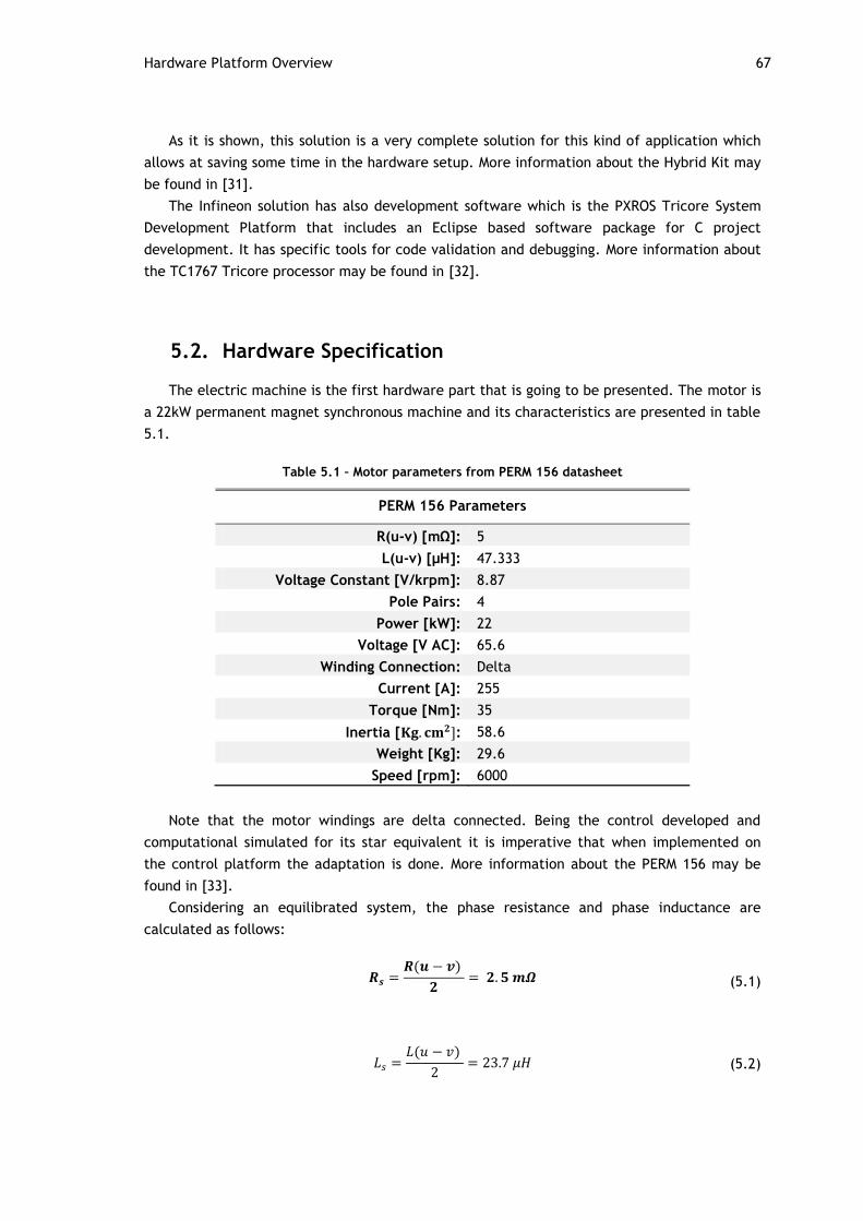
Hardware Platform Overview 67
As it is shown, this solution is a very complete solution for this kind of application which
allows at saving some time in the hardware setup. More information about the Hybrid Kit may
be found in [31].
The Infineon solution has also development software which is the PXROS Tricore System
Development Platform that includes an Eclipse based software package for C project
development. It has specific tools for code validation and debugging. More information about
the TC1767 Tricore processor may be found in [32].
5.2. Hardware Specification
The electric machine is the first hardware part that is going to be presented. The motor is
a 22kW permanent magnet synchronous machine and its characteristics are presented in table
5.1.
Table 5.1 – Motor parameters from PERM 156 datasheet
PERM 156 Parameters
R(u-v) [mΩ]: 5
L(u-v) [μH]: 47.333
Voltage Constant [V/krpm]: 8.87
Pole Pairs: 4
Power [kW]: 22
Voltage [V AC]: 65.6
Winding Connection: Delta
Current [A]: 255
Torque [Nm]: 35
Inertia [ : 58.6
Weight [Kg]: 29.6
Speed [rpm]: 6000
Note that the motor windings are delta connected. Being the control developed and
computational simulated for its star equivalent it is imperative that when implemented on
the control platform the adaptation is done. More information about the PERM 156 may be
found in [33].
Considering an equilibrated system, the phase resistance and phase inductance are
calculated as follows:
(5.1)
(5.2)
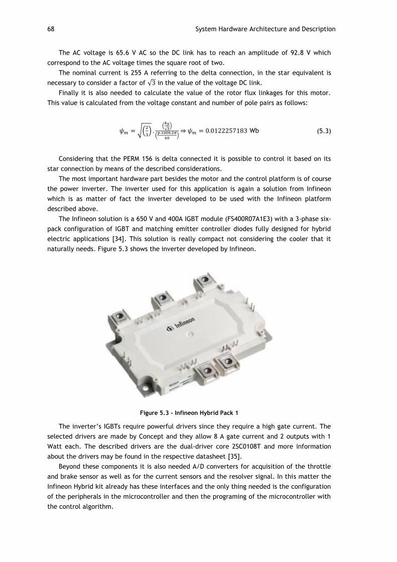
68 System Hardware Architecture and Description
The AC voltage is 65.6 V AC so the DC link has to reach an amplitude of 92.8 V which
correspond to the AC voltage times the square root of two.
The nominal current is 255 A referring to the delta connection, in the star equivalent is
necessary to consider a factor of √ in the value of the voltage DC link.
Finally it is also needed to calculate the value of the rotor flux linkages for this motor.
This value is calculated from the voltage constant and number of pole pairs as follows:
√(
)
(
√ )
(
)⇒ Wb (5.3)
Considering that the PERM 156 is delta connected it is possible to control it based on its
star connection by means of the described considerations.
The most important hardware part besides the motor and the control platform is of course
the power inverter. The inverter used for this application is again a solution from Infineon
which is as matter of fact the inverter developed to be used with the Infineon platform
described above.
The Infineon solution is a 650 V and 400A IGBT module (FS400R07A1E3) with a 3-phase six-
pack configuration of IGBT and matching emitter controller diodes fully designed for hybrid
electric applications [34]. This solution is really compact not considering the cooler that it
naturally needs. Figure 5.3 shows the inverter developed by Infineon.
Figure 5.3 - Infineon Hybrid Pack 1
The inverter’s IGBTs require powerful drivers since they require a high gate current. The
selected drivers are made by Concept and they allow 8 A gate current and 2 outputs with 1
Watt each. The described drivers are the dual-driver core 2SC0108T and more information
about the drivers may be found in the respective datasheet [35].
Beyond these components it is also needed A/D converters for acquisition of the throttle
and brake sensor as well as for the current sensors and the resolver signal. In this matter the
Infineon Hybrid kit already has these interfaces and the only thing needed is the configuration
of the peripherals in the microcontroller and then the programing of the microcontroller with
the control algorithm.

Hardware Architecture 69
5.3. Hardware Architecture
The developed algorithm discussed in the previous chapter is implemented in PSIM
simulation software in order to be computationally simulated and validated. However it is not
possible to compile the PSIM algorithm to the control platform, the algorithm has to be
adapted.
Hence, the first step for the adaptation of the developed control algorithm is to
implement the algorithm developed in the PSIM simulation software writing the
correspondent code in C language. As matter of fact, the PSIM software has also the
possibility of integrating a C block in the simulation environment which means that is possible
to replace the entire block cascade implemented for the algorithm by a C block implementing
the same control. This way it is possible to validate by computational simulating the
developed C code.
The first approach to the C code design is considering the clock period the step of the
PSIM simulation in order to obtain results on the same conditions as the ones obtained for the
PSIM block cascade implemented before. In these conditions the entire algorithm is written in
C language including the PI controllers and the Space Vector computation. Therefore the
written code is integrated in the Tricore development platform and then compiled to be
implemented on the microcontroller.
In figure 5.4 is presented a schematic where it is presented the mapping of the software
into the hardware, actually is the mapping of the computational simulation in the hardware
to be developed.
Figure 5.4 - Software into hardware mapping

70 System Hardware Architecture and Description
As is shown, the C block is mapped in the platform that can be either FPGA or the
Infineon microcontroller where the written C code will be running. Therefore the inverter
used for simulation is mapped on the Infineon inverter and the PSIM gate blocks are mapped
in the drivers for the IGBT inverter.
The resolver and the current probes represent the physical resolver and the current
sensors respectively. And finally the torque reference and the signal from the resolver have to
be acquired by A/D converters.
5.4. Conclusion
The present chapter presents a discussion about the hardware architecture as well as the
control platform considerations and specific hardware considered for the implementation.
An overview of the hardware architecture is described and the mapping of the software
into the hardware is explained in order to perform the linkage between the computational
simulation and the hardware implementation.
The following chapter presents the global results obtained after performing several
computational simulations for the developed controller written in C language. The hardware
implementation achievements are also presented and described.

Chapter 6
Global Results
This chapter pretends to discuss the overall results obtained from the computational
simulation till the system hardware validation concerning the hardware considerations
already described in the previous chapter.
In first place, it is presented several computational tests in order to analyze the behavior
and the dynamic response of the system.
Afterwards, it is presented the hardware implementation achievements carried out during
the development of the Dissertation.
6.1. Computational Simulation Results
In this section is analyzed the dynamic response of the developed algorithm implemented
in C language. The algorithm is tested for several conditions and the computational results
are presented and discussed here.
Due to the computational complexity of the system it is just presented the results for one
second of simulations. The time step defined in the PSIM simulation is seconds which
corresponds also to the clock of the C block. The program implemented in the C block runs at
each step of the PSIM simulation.
The motor parameters used are the ones presented previously in this document for its star
connection equivalent. The moment of inertia of the load is fixed in 0.3 .
The resolver sensor used has 2 pole pairs which correspond to the number of pole pair of
the real resolver that is integrated in the PERM 156. Since the PERM 156 has 8 poles, it is
necessary to introduce a multiplicative factor of 4 to obtain the real electric position of the
motor from the position signal given by the resolver.
The switching frequency is defined to 10 Khz which is a perfectly acceptable frequency
for the step time used.
The first simulation is carried out for a constant torque reference considering a time
variant load.
The computational simulation is presented in figure 6.1.
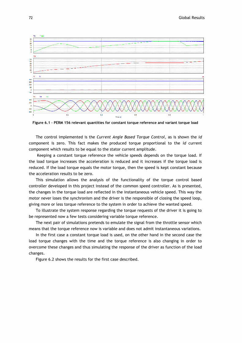
72 Global Results
Figure 6.1 - PERM 156 relevant quantities for constant torque reference and variant torque load
The control implemented is the Current Angle Based Torque Control, as is shown the id
component is zero. This fact makes the produced torque proportional to the id current
component which results to be equal to the stator current amplitude.
Keeping a constant torque reference the vehicle speeds depends on the torque load. If
the load torque increases the acceleration is reduced and it increases if the torque load is
reduced. If the load torque equals the motor torque, then the speed is kept constant because
the acceleration results to be zero.
This simulation allows the analysis of the functionality of the torque control based
controller developed in this project instead of the common speed controller. As is presented,
the changes in the torque load are reflected in the instantaneous vehicle speed. This way the
motor never loses the synchronism and the driver is the responsible of closing the speed loop,
giving more or less torque reference to the system in order to achieve the wanted speed.
To illustrate the system response regarding the torque requests of the driver it is going to
be represented now a few tests considering variable torque reference.
The next pair of simulations pretends to emulate the signal from the throttle sensor which
means that the torque reference now is variable and does not admit instantaneous variations.
In the first case a constant torque load is used, on the other hand in the second case the
load torque changes with the time and the torque reference is also changing in order to
overcome these changes and thus simulating the response of the driver as function of the load
changes.
Figure 6.2 shows the results for the first case described.

Computational Simulation Results 73
Figure 6.2 - PERM 156 relevant quantities for variant torque reference and constant torque load
In this case the torque reference does not change instantaneously for the purpose that in
the real system the torque reference is introduced by the driver and it is not instantaneous.
Here it is possible to analyze concretely the effect of the inertia of the system, note that
the produced torque starts to be smaller than the load torque and so the speed does not rise.
When the produced torque become higher than the load torque the speed continue to be zero
and it is just a few amount of time after this point that the system inertia is overcome and
the speed starts to increase.
With the Current Angle Based Torque Control the produced torque is directly proportional
to the phase current amplitude. This fact may be confirmed here since it is shown that the
phase current amplitude changes with the value of the produced torque.
The second case described above is represented in figure 6.3.
Figure 6.3 - PERM 156 relevant quantities for variant torque reference and variant torque load

74 Global Results
In this case the load torque is changing in time and the produced torque follows the
reference that here pretends to simulate the reaction of the driver to overcome the
movement opposition and maintain an approximately constant acceleration.
The torque response is really fast which allows the produced torque to follow the
reference practically instantaneously. This fact allows the driver to have a torque response as
fast as he presses or relaxes the torque sensor and this way he can give the reference he
wants to overcome the load torque and maintain the acceleration. The results of figure 6.3
illustrate what is explained before.
Note also that the ramp reference in the initial instants allows a smooth start up making
the current very small at the start up.
The previous tests are always performed for motoring operation in the forward direction.
To analyze the functionality of the motor working in reverse direction it is presented in figure
6.4 the simulating results for this operation. Note that the negative sign in the speed
indicates the reverse direction.
Figure 6.4 - PERM 156 relevant quantities for variant torque reference and constant load torque in reverse direction
The results obtained are similar to the results in figure 6.2 but this time the torque
reference is negative and the speed starts increasing in the reverse direction. The negative
sign in the speed indicates the opposite direction. Note that the torque has also a negative
signal which means that it is produced in the direction of the movement.
From the working principle point of view, the difference between these results and the
ones in figure 6.2 is just that two of the three phases are changed. In this case the phase b is
changed with the phase c.
After analyzing the PERM 156 working as a motor it is now going to be analyzed the motor
working as a generator. The regenerative braking operation is going to be computationally
tested.

Computational Simulation Results 75
Figure 6.5 represent the results for the regenerative braking operation.
Figure 6.5 - PERM 156 relevant quantities for regenerative braking operation
In first place the motor is accelerating introducing a positive reference of torque and the
speed increases. Therefore, a torque reference with opposite signal to the movement is given
to the controller. Note that this reference is given by means of a ramp in order to smooth the
transition.
When the produced torque has signal in opposition to the movement the average power
changes its signal indicating the change in direction of the power flow. From this point
forward the motor is working as generator feeding the system with current to charge the
storage system. The speed starts decreasing and hence is proved the functionality of the
regenerative braking.
In figure 6.6 is represented the results for a simulation where the motor is accelerated
then braked and accelerated again.
Figure 6.6 - PERM 156 relevant quantities for motor operation and regenerative braking operation

76 Global Results
Analyzing the obtained results it is confirmed that the power flow changes signal every
time the torque is against the movement. The speed increases when the produced torque is in
favor of the movement and decreases when the torque is against the movement.
Note then when the motor is working as a generator the stator current vector is lagging
the air gap flux vector contrarily to what happens during motor operation where the stator
current vector is leading the air gap flux vector.
6.2. Hardware Implementation Achievements
This section describes the hardware implementation achievements concerning the
implementation of the C algorithm created in the analyzed control platforms.
Concerning the FPGA platform the first approach is to adapt the developed algorithm and
adapt it to VHDL language. This process would take much time and it is decided to create the
VHDL code by means of automatic generation code. Matlab Simulink software presents a tool
named HDL coder that allows the generation of VHDL code from the generic Simulink blocks.
The developed control algorithm is presented in figure 6.7.
Figure 6.7 - Traction control algorithm developed in Matlab Simulink
The control loop is adapted from the PSIM control loop including the space vector
computation that is implemented inside of the subsystem block and it is represented in figure
6.8.

Hardware Implementation Achievements 77
Figure 6.8 - Space Vector computation subsystem implemented in Matlab Simulink
Note that the algorithm has already some adaptations concerning the requirements of the
HDL coder. The selected simulation solver is defined to discrete with fixed-step and some
functions and blocks are changed like the case of the arctangent block that had to be
substituted by a look up table due to incompatibilities of the block with the HDL coder tool.
The other trigonometric functions as the sine and cosine functions are defined to its CORDIC
approximations.
Although all the adaptations carried out to work with the HDL coder some crucial blocks
are not compatible with the tool even defining the blocks to work with fixed-point and some
errors occurred making the implementation based on this tool very difficult.
It is so decided that the best solution concerning the implementation of the algorithm in
the FPGA regarding of the scope of this Dissertation is the implementation of the soft
processor core based architecture as described in the previous chapter. This way the C based
control algorithm can be used to program the soft-processor core. Besides that, the algorithm
is portable considering also its implementation on the microcontroller based Infineon
platform.
The first approach for the adaptation of the algorithm is simply the compilation of the
created C code in the development tools of each platform. After a small code adaptation the
code is successfully compiled which validates the created control program.
In the case of the Infineon solution the code is adapted and compiled in the Code::Blocks
platform IDE which is the compiler for the Infineon Tricore microcontrollers.
Regarding of the FPGA implementation, the first step is the implementation of the
MicroBlaze soft processor. Xilinx Platform Studio or XPS for short is the software tool where
the MicroBlaze hardware and software is developed. It has an editor and project manager
interface for source code creation and edition. Furthermore the Xilinx Embedded
Development Kit tools have a built in C compiler that allow the generation of the necessary
machine code for the processor. Using the Base System Builder tool of the XPS a project is
created and information about the Xilinx board to use has to be discriminated. Therefore, the

78 Global Results
tool allows the setup of the number of processing units and then a processor configuration
dialog box is presented for further configurations.
The processor clock frequency and bus clock frequency are setup to 50 Mhz which is the
frequency of the Xilinx Sparten-3E crystal. The local data and instruction memory are
defined to 16 KB. Finally the internal peripherals are added to the processor.
After the configuration is done a C source file is created and the developed C code is
integrated here concerning the changes related with inputs and outputs. The necessary
peripherals have to be also added to the project and finally the project may be compiled and
the machine code generated.
6.3. Conclusion
The overall results are presented and analyzed in this chapter. It is demonstrated that the
best control for the considered motor is the Current Angle Based Torque Control that
pretends to control the produced torque based on the amplitude of the stator current
amplitude since the torque is directly proportional to it. The results performed for
regenerative braking operation are also presented and described.
Finally, the chapter describes the first approaches to the hardware implementation based
on two different platform solutions.
The following chapter presents the overall conclusions and introduces further
developments to perform giving continuity to this project.

Chapter 7
Conclusion
The present chapter is the final chapter of this document and it pretends to summarize
and discuss the final conclusions about the developed work.
Furthermore, it is discussed the future work to be developed in order to give continuity to
the work already developed within the master Dissertation.
7.1. Dissertation Conclusion
Researches and projects developed during the past years present different solutions and
approaches to the electric and hybrid electric technologies. Treating all of the aspects and
subsystems of a hybrid electric vehicle carefully is a complex and time consuming task to be
developed on behalf of a Master Dissertation. Considering this fact, the proposed problem of
this Dissertation is focused just on the electric traction system unit of a HEV. Allowing a
focused and complete analysis of the question in a scientific and practical point of view.
The State of the Art chapter presents an overview of the current technology in the matter
of HEVs, allowing the introduction and familiarization with the subject, focusing in aspects as
the overall architecture of the system, the different kinds of electric machines, the inverter
configuration and finally the control platform solution.
The System Modeling chapter aims to discuss the dynamic modeling of the system in order
to understand how it works and how it can be potentially controlled. The working principle of
the PMSMs is explained and the equations that model the motor dynamically are presented as
well as the mechanical equation that models the mechanical part of the system. It is also in
this chapter that a scientific analysis about the notion of the torque is conducted discussing
the several approaches presented among the literature. Although, the different approaches
are never considering the same angle it is justified why each approach can be used as the
torque angle from a control point of view.
Starting from what is learned from the analysis carried out regarding of the subject of the
System Modeling chapter it is presented in the System Controller Design the architecture of
the controller designed and the developed methods in order to create the most suitable
control for the purposes of the Dissertation problem. Several methods for the electric

80 Conclusion
traction control loop are presented and discussed regarding of its application in the control
not just for a particular type of motor but including different kinds of PMSMs attempting to
present a wide analysis of the question. It is demonstrated that the best control regarding of
the maximization of the Torque/Current ratio is the developed Maximum Torque per Ampere
Control for the case of PMSM with . On the other hand, for the case of PMSMs with
the control method showing the best results is the Current Angle Based Torque
Control. Considering the PERM 156 as the solution for the hardware implementation, it is
possible to successfully implement a PSIM simulation schematic modeling the system
integrating the PERM 156 allowing the comparison of the several control methods developed.
Finally, the chapter presents the developed software architecture for the high level algorithm
of the electric traction system unit.
In the System Hardware Architecture and Description chapter is discussed the considered
solutions for the hardware architecture and its implementation. The solutions for the
inverter, drivers and motor are presented and discussed. Finally, two solutions for the
controller are considered and discussed one of them is a microcontroller based solution
specially designed for the purpose where just the software is needed to be developed. On the
other hand, the other one is a FPGA based solution which the architecture has to be defined
and implement from the root.
Finally, the Overall Results chapter presents the validation of the system based on the
computational simulation results and hardware implementation achievements. The developed
C algorithm is simulated in the PSIM software and its results are presented and analyzed. The
control method implemented is the Current Angle Based Torque Control since it is the one
showing the best results. The simulation results are very consistent proving the robustness of
the controller regarding of the stability of the system maintaining the synchronism of the
machine and a very fast torque response. The regenerative braking is also object of
simulation. The results are presented and analyzed. It is demonstrated the power flow
changes its signal when the motor is braking the system. Hence, it is validated by means of
computational simulating the functioning of the control system for the motor working as
motor and generator.
In the Overall Results chapter is also presented the achievements in what respects the
hardware implementation. They are presented the first approaches of the implementation of
the algorithm by compiling the code in the respective development platforms. For the FPGA
based controller it is also explained the implementation of the MicroBlaze soft processor
core. Unfortunately it is not possible to attain further developments regarding of the
hardware implementation and prototype testing in time. The hardware assembly and the
familiarization with the control platforms like a FPGA require a considerable amount of time
dedicated to its study which is difficult to achieve within the development of the master
Dissertation.
Although the prototype construction stage is not possible to attain, the dedication to the
study and design of the controller based on the deep analysis of the working principles of the
permanent magnet synchronous machines made possible the development of a robust control
algorithm that is validated by means of computational simulation. This fact together with the
conducted study regarding the solutions for hardware constitutes a solid basis for further
implementation of the system.

Further Developments 81
7.2. Further Developments
The present Dissertation constitutes a solid starting point for the implementation of the
electric traction system unit for an electric or hybrid electric vehicle. The control algorithm
is ready to be implemented and the source code is validated for the considered platforms.
The work to be developed henceforward is in first place the implementation of the
further FPGA configuration related with the software and hardware for signal acquisition. In
the case of the Infineon solution it is just missing the software configuration of the
acquisition hardware since the hardware part is already configured in this solution.
The next stage is thus the signal conditioning and hardware assembly in order to setup a
prototype to be tested in a laboratory environment. The space vector algorithm has to be
adopted as is mentioned in chapter 5 considering the delta connection of the motor. If the
system is validated in the laboratory, it is ready to be integrated in the hybrid electric vehicle
together with the other units. Note that the interface of the motor shaft with the
transmission is also a subject of analysis. It has to be developed a solution for the mechanical
coupling that may include direct coupling or fixed gear relation and also transmission with
electronic clutch. This fact will have impact on the speed range of the motor and so further
configurations and adaptations of the algorithm may have to be done.
Furthermore the interaction between the electrical brake and mechanical brake is also a
subject of study and further development. It is really important that the brake security is
ensured.
There are also some software alterations to be done in the traction control algorithm
concerning the communication with the Energy Management Control Unit. It is necessary to
define how the communication is going to happen and implement conditional structures that
manage the functioning of the electric traction system in concordance with the current state
of charge. In other words, whether the system can or cannot regenerate energy from braking
or if it has to limit the power in order to extend the range of the trip.
Finally, there are several improvements that may be added to the system regarding the
energy balance of the system. One of the improvements born from the complications of
calculating the range of the vehicle considering the electric energy needed for traction and
the energy recovered. Hence, a GPS based solution may help predicting the amount of energy
going to be spent and the amount of energy that is going to be possible to regenerate
allowing a more accurate energy balance calculation that will reflect a more precise
predicted range.


References 83
References
[1] I. Xilinx, "Programmable Logic Design," 2008.
[2] R. Krishnan, Electric motor drives: modeling, analysis, and control: Prentice Hall,
2001.
[3] M. Ehsani, Y. Gao, and A. Emadi, Modern electric, hybrid electric, and fuel cell
vehicles: fundamentals, theory, and design: CRC Press, 2009.
[4] N. Hashemnia and B. Asaei, "Comparative study of using different electric motors in
the electric vehicles," in Electrical Machines, 2008. ICEM 2008. 18th International
Conference on, 2008, pp. 1-5.
[5] X. D. Xue, K. Cheng, and N. C. Cheung, "Selection of eLECTRIC mOTOR dRIVES for
electric vehicles," in Power Engineering Conference, 2008. AUPEC '08. Australasian
Universities, 2008, pp. 1-6.
[6] Z. Q. Zhu and D. Howe, "Electrical Machines and Drives for Electric, Hybrid, and Fuel
Cell Vehicles," Proceedings of the IEEE, vol. 95, pp. 746-765, 2007.
[7] L. V. Cardoso, "Desenvolvimento de'Range Extender'para veículo eléctrico," Porto,
FEUP, 2011. Dissertation.
[8] S. M. N. Hasan and I. Husain, "Power electronic interface with ultracapacitors and
motor control for a fuel cell electric vehicle," in Vehicle Power and Propulsion, 2005
IEEE Conference, 2005, pp. 815-822.
[9] M. Ehsani, G. Yimin, and S. Gay, "Characterization of electric motor drives for
traction applications," in Industrial Electronics Society, 2003. IECON '03. The 29th
Annual Conference of the IEEE, 2003, pp. 891-896 vol.1.
[10] C. C. Chan, "The state of the art of electric and hybrid vehicles," Proceedings of the
IEEE, vol. 90, pp. 247-275, 2002.
[11] M. Ehsani, G. Yimin, and J. M. Miller, "Hybrid Electric Vehicles: Architecture and
Motor Drives," Proceedings of the IEEE, vol. 95, pp. 719-728, 2007.
[12] H. C. Lovatt, D. Elton, L. Cahill, H. Duc Hau, A. Stumpf, A. Kulkarni, A. Kapoor, M.
Ektesabi, H. Mazumder, T. Dittmar, and G. White, "Design procedure for low cost, low
mass, direct drive, in-wheel motor drivetrains for electric and hybrid vehicles," in
IECON 2011 - 37th Annual Conference on IEEE Industrial Electronics Society, 2011, pp.
4558-4562.
[13] I. Boldea and S. A. Nasar, Electric drives: CRC/Taylor & Francis, 2006.
[14] B. P. Kumar, "DSP Hardware Design I," in Digital Signal Processing Laboratory, ed: CRC
Press, 2005, pp. 103-143.
[15] K. Ying-Shieh, "Design and Implementation of a High-Performance PMLSM Drives Using
DSP Chip," Industrial Electronics, IEEE Transactions on, vol. 55, pp. 1341-1351, 2008.
[16] S. Hasan, "Hybrid electric vehicle powertrain: On-line parameter estimation of an
induction motor drive and torque control of a PM BLDC starter-generator," The
University of Akron Ph.D., The University of Akron, United States -- Ohio, 2008.
[17] R. de Castro, R. E. Araújo, and D. Freitas, "FPGA Based Powertrain Control for
Electric Vehicles," Electric Vehicles-Modelling and Simulations, 2011.
[18] A. Corporation. 2011, Optimize Motor Control Designs with an Integrated FPGA Design
Flow. [Tecnical Document].
84 References
[19] L. Hak-Jun, S. Hojoon, S. Seung-Ki, K. Sang-Min, and P. Yongho, "System configuration
and control strategy using FPGA for Hybrid vehicle power Control Unit," in Power
Electronics and ECCE Asia (ICPE & ECCE), 2011 IEEE 8th International Conference on,
2011, pp. 1696-1702.
[20] G. McPherson, An introduction to electrical machines and transformers: Wiley, 1981.
[21] B. Nicola, "Permanent Magnet Synchronous Motors," in Power Electronics and Motor
Drives, ed: CRC Press, 2011, pp. 1-46.
[22] Z. Yan, "Control and Observation of Electric Machines by Sliding Mode," Ohio, Ohio
State University, 2002. Dissertation.
[23] A. Emadi, Handbook Of Automotive Power Electronics And Motor Drives: Taylor &
Francis, 2005.
[24] M. Kazmierkowski, "Control of Converter-Fed Induction Motor Drives," in Power
Electronics and Motor Drives, ed: CRC Press, 2011, pp. 1-39.
[25] B. K. Bose, Power Electronics And Motor Drives: Advances And Trends:
Elsevier/Academic Press, 2006.
[26] V. Blasko, "A hybrid PWM strategy combining modified space vector and triangle
comparison methods," in Power Electronics Specialists Conference, 1996. PESC '96
Record., 27th Annual IEEE, 1996, pp. 1872-1878 vol.2.
[27] S. Kouro, J. Léon, L. Franquelo, J. Rodríguez, and B. Wu, "DC?AC Converters," in
Power Electronics and Motor Drives, ed: CRC Press, 2011, pp. 1-50.
[28] T. Sá, "Traction Control in Electric Vehicles,", Porto, FEUP, 2012. Dissertation. To be
Published.
[29] I. Xilinx, "Spartan-3E FPGA Starter Kit Board User Guide," vol. UG230 (v1.2), January
20, 2011 2011.
[30] I. Xilinx, "MicroBlaze Processor Reference Guide " vol. UG081 (v11.2), 2010 2010.
[31] I. T. AG, "Hybrid Kit for HybridPACK™1 Evaluation Kit for Applications with
HybridPACK™1 Module," vol. V2.5, 2012-03-30 2012.
[32] I. T. AG, "TC1767 32-Bit Single-Chip Microcontroller," vol. V1.1 2009-05, 2009.
[33] H. G. C. KG, "Heinzmann Product Catalogue Disc Motors," 2012.
[34] I. T. AG, "HybridPACK™ 1 - Power Module for Hybrid- and Electric Vehicles," 03 / 2012
2012.
[35] C. T. AG, "2SC0108T2Ax - 17 Preliminary Data Sheet," 2009.
