529

SOME CURRENT APPROACHES TO EDITING IN THE ABS

Keith Farwell and Mike RaineAustralian Bureau of Statistics, GPO Box 66A, Hobart, Tasmania, 7001

email: keith.farwell@abs.gov.au, mike.raine@abs.gov.au

The views expressed in this paper are those of the authors and do not necessarily reflect those of the AustralianBureau of Statistics (ABS).

ABSTRACT

A number of ABS collections have implemented editing strategies based on ‘significance’ criteria. This editing approachattempts to rationalise resource usage through prioritising editing activity based on measures of its impact on estimates. Morerecently, considerable attention has been given to the management of ‘respondent load’. Taken together, a logical model forprocessing built around managing respondent contact has evolved.

The Agriculture Program is currently designing a system which will embed these concepts into an integrated processingsystem. If successful, the system will form a prototype for more general ABS use. This paper will present some results ofinvestigations and experience developing a practical implementation of these concepts.

Key Words: Quality, Significance, Score, Benefit, Respondent burden, Quality monitor, Collection model

ACKNOWLEDGEMENTS: The authors wish to acknowledge the valuable comments and suggestions provided byRobert Poole during the development of this paper.

1. INTRODUCTION

There has been a consistent thrust at the ABS to reduce survey costs, deliver more timely statistics, and minimiserespondent burden. Gains in these areas can often be found through refining the editing process.

In the past, output editing systems within the ABS have often struggled to identify quickly the unit responsesresponsible for questionable output. The statistical aspects of output editing are concerned not only with detectingany remaining influential erroneous data, but also with identification of outliers and analysis and explanation ofsurvey trends. A desirable statistical output editing system would be one which could quickly detect influential dataand prioritise those which, when investigated, result in acceptable output which can be explained.

Studies within the ABS and other statistical agencies have shown that ‘classical’ input editing systems have tended togenerate too many edit failures. Too much time and effort was spent querying unit records. Often, resolution of onlya limited number of edit failures resulted in any meaningful change to estimates. These editing strategies did noteffectively target those responses most worth pursuing. A desirable input editing system would be one which couldaccurately detect erroneous data and prioritise those which, when resolved, result in meaningful changes to estimates.

This paper traces the development of significance-based editing within the ABS. References are made to someprojects that have helped shape our view of significance-based editing. In Section 7, the paper takes a step awayfrom the methodological viewpoint and illustrates some of the practical issues involved with implementing thestrategy for the Agriculture Program.

2. GENERAL USE OF SIGNIFICANCE CRITERIA IN EDITING

Editing activity can be maximised with respect to cost by confining our attention to the most significant units. Thisapproach can be used at both the input and output stages. The streamlining of these activities will assist with thetimeliness of data quality operations and can be used to control and minimise respondent re-contact.

Relating impacts on estimates to the targetting of survey processing activity can have a beneficial effect on subjectmatter areas. It can be a catalyst for a better understanding of the statistical and sampling processes. The fundamentalstatistical concepts of estimation, estimation weights, and representation are used and drawn into day-to-day

530

activities. The concepts can underpin input editing, output editing, output analysis, outliering, and other processessuch as intensive follow-up procedures.

A measure of significance can be used to derive a ‘score’ to rank item responses or respondents and those withhigher ranks should be those we target for closer scrutiny (Latouche and Berthelot 1990). We need to address twokinds of editing significance depending on whether the focus is on input editing or output editing (Farwell 1991). Foroutput editing, we are primarily interested in a unit’s actual contribution to an estimate and significant units are thosewith high contributions to estimates. For input editing, we are most interested in erroneous data which, whencorrected, induce important changes in estimates and significant units are those we expect to have a high impact onthe change in an estimate due to editing activity. In this paper, input editing based on significance criteria will becalled ‘significance editing’ while output editing based on significance criteria will be called ‘statistical outputediting’. Significance criteria can also be used as a basis for reviewing and assessing an existing editing system. Forexample, editing bounds can be modified in an objective manner and edit performance can be quantified.

It would be advantageous if significance measures use only a minimal amount of auxiliary information. For example,information on the current unit (including historical if available) and a small store of common information (such asthe current and previous estimates). The measures should be based on simple statistical techniques that are quick andinexpensive (so as not to unduly slow the editing process). The measures should have a similar form regardless of thecomplexities of the estimation system and should be consistent with the type of estimates being produced.

2.1 Local and Global Ranks

Scores and ranks relating to item responses (or particular estimates) can be considered as ‘local’ measures. Thoserelating to the complete return can be considered as ‘global’ measures. If we have a number of items of interest, ascore can be calculated separately for each of these items (for each unit). We would like to have just one score foreach unit rather than a separate score for each item of interest. Each type of ranking approach has certain advantagesand it would be expected that both would be used.

A local ranking will be based on a set of specific data items within a unit record and will tend to target a specificestimate. The disadvantage with a local rank is that a unit record can have different rankings for different estimates.A unit record may be considered worthy of scrutiny for one type of estimate but not for another.

A global ranking attributes significance at the unit level rather than the item level. Use of a global ranking will assistto control the number of respondent records requiring examination. Using both types of ranking would give somecontrol over the conflicting constraints of minimising respondent recontact while maximising the editing benefit.

There are many ways one might develop global scores. Local scores usually need to be standardised prior toassimilation. If we wish to give some items more influence than others we could give each local score a weightreflecting our assessment of each local score’s relative importance before combining them into a global score.

3. USE OF SIGNIFICANCE CRITERIA IN OUTPUT EDITING

Output editing is performed when we want to finalise estimates — when it is considered that the response rate issufficiently large, that basic errors have been fixed, and dissemination deadlines approach. Any remaining largeerrors need to be found. Outliers are detected and estimates are analysed in terms of trend and quality.

Output cells that require further investigation are usually detected by a combination of methods. Some methods aresubjective, such as ‘eye-balling’ the estimates for unexpected behaviour or comparing the estimates with informationfrom other sources. Some methods can be automated, such as choosing cells with large movements or with largerelative standard errors. Once the cells requiring interrogation have been found, we investigate those respondents thatwe consider to be highly influential to the estimate (which can include aspects such as the change from the previousestimate, or the relative standard error of the estimate).

Local scores based on unit contributions to estimates can be used in output editing. For an estimate of level of theform X = Σ wi xi, the unit contribution to level is simply wi xi (where wi is the estimation weight and xi, the item

531

response for respondent i). If the estimate of movement is the difference between estimates at two time points, theunit contribution to movement is the difference between the two unit contributions to level. Non-linear estimatessuch as estimates of ratio (X/Y, where Y = Σ wi yi) can be linearised by methods such as Taylor Series Expansionapproximation or the ‘drop-out’ method (where the impact is the difference between the estimate with, and without,the contribution included). For example, the drop-out method approximates the unit contribution to the ratio X/Y withwi (xi Y - yi X)/[Y (Y - wi yi)] and results in the unit contribution to a difference of ratios is the difference between theindividual unit contributions to the ratios. Unit contribution to the variance of an estimate can also be calculated.

Even at the item level, several scores can be calculated. For example, we could use unit contribution to level,movement, and variance for a single item. Unit contribution to level can be biased as an editing tool because it willnot highlight units with response values that are too small. However, it is useful for highlighting large contributorsand outliers, problem strata, and incorrect weights. The contribution to movement score is useful for discoveringerratic responding behaviour and is the starting point for analysis of movements. The contribution to variance scorecan highlight inconsistent behaviour and tie in the effect of benchmarks, sampling frames, and poor response rates.

Editors are often interested in the local scores when expressed relative to the estimates they target. For example, therelative unit contributions for level and movement are:

OL,i = wi xi / | X |, andOM,i = (wt,i xt,i - wt-1,i xt-1,i) / | Xt - Xt-1 |, where t and t-1 refer to time periods.OV,i can also be derived for variance.

The above scores need to be combined into an item score and then different item scores should be combined into aglobal score to prioritise respondent level activity. The relative scores might require further modification. The‘variance’ score should be restricted to only those respondents that participate in the activity of interest for editingpurposes. For example, some items can be both positive and negative and this can lead to problems later.

We define ‘benefit’ as the absolute value of a score. Relative benefit for level and movement are:

BL,i = | wi xi | / Σ | wi xi |, andBM,i = | wt,i xt,i - wt-1,i xt-1,i | / Σ | wt,i xt,i - wt-1,i xt-1,i |.BV,i can also be derived for variance.

Careful consideration is required to develop global scores and the methodology is dependent on the main surveyobjectives. There are a variety of ways that a group of local relative benefits may be combined. Some starting pointsare to use the score for the most important variable or use the largest of the item scores as a proxy for the globalscore; use item weights in conjunction with the scores; use a ‘distance’ measure; use a combination of ranking andscoring; etc. For example, an item level benefit for a unit might be BI,i = square root (BL,i

2 + BM,i2 + BV,i

2).

The local or global significance measures can be used to identify and rank highly influential responses. Some of thehighlighted responses might contain errors which require correction while others might contain correct data. Thosewith correct data usually become contenders for outliering activity. Scrutiny of the unit impacts can help in theanalysis and explanation of the survey results.

3.1 Statistical Output Editing in the Agricultural Finance Survey (AFS)

The annual AFS is a random sample of 2,500 farm businesses designed to collect a fixed set of financial data.Rotation of units into and out of the sample is controlled so that about one third of the sample is new units. Estimatesof magnitudes are produced using within stratum ratio estimation with the estimated value of agricultural operationsas benchmark while estimates of population sizes are produced using number raised estimation. Statistical outputediting has been used as the main editing method since 1992. Very little input editing is done — only various logicaland consistency edits are used.

532

Survey respondents are separately ranked according to the absolute values of their contributions to the estimate oflevel, the movement between consecutive estimates of level, and the variance of the estimate. The movement score iscalculated for continuing units only. Contributions to level lists are useful for dealing with new units in AFS and forquick identification of outliers.

The main editing run produces separate rankings for four ‘indicator’ items — turnover, purchases and expenses,value of assets, and net indebtedness. It is considered that many problems with other items will often be detectedthrough investigating the indicator items. Indicator items were used to keep the number of lists to a manageable size.Specific runs can be done for user-defined items. For example, any estimates that have movements or RSEs greaterthan 10% at the Australian level are investigated.

The top fifteen contributors are listed at Australian, State, and Industry levels. A final list of outlier contenders isproduced by manually inspecting the lists of local rankings. It was considered that the lists could be combinedmanually because the volume of material to look through was manageable and there was not a strong need to attemptto combine local ranks or to produce global ranks.

AFS found this output editing approach very effective and less time was needed for editing activity. Staff developeda better working knowledge of the statistical process (such as a better understanding of estimation weights, outliers,and movements). Various aspects of the analysis of survey results could be commenced as part of the editingprocess. For example, documentation of the results of editing investigations (such as recording why a highlyinfluential response was left untouched) could feed into the analysis of survey results. AFS were able to bring theirpublication deadline forward by a month as a result (so that estimates were finalised within 13 months of thereference period).

3.2 Statistical Output Editing in the Agricultural Commodity Survey (ACS)

The basic statistical output editing approach used in AFS is being extended in the current 1998/99 ACS. The annualACS is a random sample designed to collect agricultural commodity data from farms and uses number raisedestimation. Editing in ACS has different problems to those in AFS.

The inaugural 1997/98 ACS (it was a census of 140,000 farms previously) was a sample of 63,000 farms but the1998/99 sample was cut to 35,000. The change in sample size caused problems with the contribution to movementscore. The sample size change generated large increases in sampling weights. It was possible for a continuing unit tohave a large movement score even when its responses are identical for both years. To identify questionableresponses, we needed to exclude the impact of changes in weights. This was done by noting that wt,ixt,i - wt-1,ixt-1,i canbe expressed as wt,i(xt,i - xt-1,i) + (wt,i - wt-1,i)xt-1,i and, using the first term on the right as an alternative measure for themovement score, OM,i = wt,i (xt,i - xt-1,i) / | Xt - Xt-1 |.

ACS does not collect a fixed group of data items from any one respondent. It is common for an ACS respondent toreport more than 20 commodities and the mixture of commodities varies between respondents. There are over 900commodities Australia-wide. Therefore, the use of indicator items does not help to reduce the number of listsgenerated for ACS. Statistical output editing is augmented by other editing processes which identify output cells thatrequire further attention. There are various methods that can be applied for identifying these cells.

ACS has a larger proportion of new units than AFS. Rotation of units into and out of ACS is not controlled and theproportion of new units is expected to be up to three in four in future years (whereas it is about one in three for AFS).Therefore, new units and contributions to movement are more of a problem than for AFS.

A commodity benefit is currently used in conjunction with the relative local scores for level, movement and variance(where units are ranked for each). Currently, the commodity score is adjusted to account for the problem with themovement score for new units by doubling the impact of the variance contribution:

BI,i = square root (BL,i2 + BM,i

2 + BV,i2 ) for continuing units, and

= square root (BL,i2 + 2 BV,i

2) for new units.

533

This early version of the ACS statistical output editing system is being improved and extended within the newAgriculture system being developed by the Agriculture Re-engineering Team. For example, the current system doesnot use a unit level score. This is a key element of the new system and work is underway to develop this score.

4. USE OF SIGNIFICANCE CRITERIA IN INPUT EDITING

This section deals with the notion of targetting only those responses worth pursuing within an input editing context.A significant unit to edit is one which, if treated by amendment, would lead to an important change to an estimate.Obtaining a corrected value through clerical action is expensive (particularly if respondent recontact is involved) andthe effort is wasted if the resulting actions have only a minor effect on estimates. Conversely, if there were a largechange in the estimates, clerical attention would have been worthwhile. The targetting of only the significant editfailures for clerical attention is called ‘significance editing’ (Lawrence and McDavitt 1994) within the ABS. Ratherthan attempting to correct all reporting errors, significance editing attempts to target editing resources towardsresponses which are likely to provide the largest reduction in reporting bias in estimates.

A theoretical framework for significance editing is being developed which uses a super-population approach tomodel the effect of editing. For the case of a single estimate, the work has looked at the problems of minimisingreporting bias for a fixed cost and minimising cost to achieve a fixed level of reporting bias. Preliminary resultsshow that, in the case of uniform cost per unit, both problems have analytical solutions and that only numericalsolutions are possible if the cost per unit is not uniform. The following score for an estimate of level was shown to bean appropriate choice for a local significance score under the postulated model (Poole 2000; Carlton 1999).

For an estimate of level of the form X = Σ wi xi, the expected unit contribution to change can be approximated bywi qx,i Dxi, where Dxi = xi* - xi; xi* is our expected or imputed value for the response (xi); and qx,i is the probabilitythat the response is erroneous for item x. Non-linear estimates such as estimates of ratio need to be linearised beforethey can be expressed as sums of unit contributions. For example, the unit contribution to X/Y can be approximatedby wi (qx,i Dxi Y - qy,i Dyi X) / [Y(Y + wi qy,i Dyi)] using the drop-out method.

Local scores based on contributions can be expressed relative to the estimates that they target. This has the advantageof indicating the likely impact on an estimate. Scores expressed relative to standard errors may be more appropriatewhen reported values can be both positive or negative. Local relative scores for estimates of level and rate are:

SL,i = 100 (wi qx,i Dxi) / | X |, andSR,i = 100 wi (qx,i Dxi Y - qy,i Dyi X) / [ | X |(Y + wi qy,i Dyi)] if Y > 0

= -100 wi (qx,i Dxi Y - qy,i Dyi X ) / [ | X |(Y + wi qy,i Dyi)] if Y < 0.

The major difficulty with this approach is that we need to form an expectation of the likely impact due to editing inisolation of other responses. At the stage of processing when input editing is usually done, many of the responsesfrom the final sample will not be known and information such as the final estimation weights, the values of finalestimates, and attributes such as sample means would not be known — approximations are needed. For example,design weights and previous estimates (with an adjustment accounting for expected growth) can be substituted forestimation weights and expected current estimates.

The second difficulty involves estimating appropriate ‘qi’ values. This might be done at unit by item level or higher.For example, new units in the survey or units in a particular sector of the population might tend to be more likely tomisreport. Alternatively, we might assume that all responses are erroneous and assign qi = 1 (to date, ABS has usedqi = 1 for simplicity). It is not yet clear whether the qi term introduces any practical improvement to the eventualrankings but, technically, it is needed to generate a more accurate estimate the expected benefit due to editing.

Item responses can be ranked through a benefit measure based on the local scores. A system is required to impute thelikely response value for each responding unit which must be independent of response rate. If a useful estimate oflikely change is not achievable, we might be able to find a measure which is associated with the likely change. Forexample, the benchmark size, the sampling weight, or the severity of an edit failure might be useful.

534

This significance-based strategy can be used as a stand-alone editing system or, if we do not wish to discard anexisting input editing system, we can apply significance criteria to the edit failures produced by the system. Since anedit (or group of edits) will often target a specific estimate, a local ranking will usually coincide with the recordfailures from a specific edit (or group of edits). Otherwise, the local scores might need to be combined for thispurpose. Either way, scores can be developed for the failures from specific edits. We can prioritise the input editfailures using the significance scores. A ‘cut-off’ can be used where data with a benefit value above the cut-off areexamined — other data is ignored or imputed.

Cut-off values could be determined through empirical investigation for repeating surveys or they might be modelledfor infrequent surveys. In setting cut-offs we need to balance the bias due to not editing some units with the gains ofediting others. Note that the effectiveness of significance editing relies on there being a reasonable number of unitshaving an insignificant collective impact due to editing. Modelled cutoffs can be derived by assuming that the meanscore of unedited units is zero (i.e. E(Si) = 0 ) and that response errors are independent. Say that a cut-off value awas chosen and that na units will not be edited. It can be shown that, for an estimate X, E[Bias2(X)] = na E[Si

2]. Ifthe Si are uniformly distributed on [-a, a], E[Si

2] = a2/3, and we can set E[Bias2(X)] = k Var(X) or k X2 for some k<1(Lawrence and McKenzie 1999). These might be reasonable initial cut-offs which can be modified if necessary.

In order to control the number of re-contacts necessary to achieve the desired quality in the estimates, global scoresand rankings are needed. Various global scores have been suggested but no clear guidelines exist for these. Someconsiderations include the survey objectives, the relative importance of estimates and the volatility of the data.

4.1 Use of Significance Editing in the Survey of Average Weekly Earnings (AWE)

Significance editing has been used in AWE since 1992. AWE is a quarterly survey of approximately 5,000businesses from a population of about 600,000. There is a high proportion of continuing units (about 90% perquarter). The significance editing approach is superimposed on the existing input editing system and is applied tocontinuing units but not new units. Historical information is used for imputation purposes. New units are handleddifferently, not only because of the lack of historical information (other imputation methods are possible), butbecause it was believed that there are benefits in separately editing new units since it is expected that they wouldhave a higher error rate. New units are only a small proportion of both the sample and the editing workload.

The items of interest are a number of wage to employment ratios for various categories of units. The score for ratios,SR,i (as defined in Section 4), is used with qi = 1 for all variables. Local scores are calculated for five of the ninevariables collected. A unit score is defined as the maximum of the local scores and cut-offs are defined separately foreach State (Lawrence and McDavitt 1994). Ranking units at State level was preferred to Australian level because itgave better results at State by industry level. The last quarter’s return is used to estimate an expected value. It wasfound that the previous return did not require adjusting by a growth rate. A simulation study found that the rankingswere reasonably insensitive to variations in growth rate.

Empirical investigations indicated that cut-offs should be chosen in order to target the top 40% of the input editfailures from the existing system. It was found that input editing (using significance editing) could be done withabout 80% of the staff that had previously been required. There was no noticeable change in the estimates.

4.2 Use of Significance Editing in the Survey of Employment and Earnings (SEE)

SEE is a quarterly survey of approximately 12,000 businesses (from about 600,000 businesses). Employment andearnings information is collected. A similar significance editing approach to AWE is being planned. Significanceediting cutoffs were specified using the model-based approach outlined in Section 4 where a value of k =0.1 wasused in conjunction with variance.

It is intended that significance editing will be applied only to continuing units that fail input query edits. Units thatare permanently nil or defunct, new to the survey, did not fail an edit, or failed fatal edits will be excluded. New unitswill be separately examined and dealt with. All fatal edit failures will be examined. Query edit failures for units withscores less than the cutoff will be forced clean.

535

Investigations indicate that the amount of input edit failures requiring investigation can be reduced by 40% to 50%while having no noticeable effect on the survey results. Resources saved (expected to be 20% to 25%, or 2 to 3 staffyears) during input editing can be better spent analysing and understanding the survey results (Lawrence 1999).

5. APPLICATION OF SIGNIFICANCE EDITING WITH A COMPLETE RESPONDENT FILE

If timetables permit and a survey team prefer to wait until later in the collection cycle before initiating any editingaction, it is possible to make more effective use of (input) significance editing. For example, preliminary results areoften required before the end of a cycle and these estimates will be based on the available respondent data (that is,most of the units that we wish to input edit are present). Generally, there will be a need to quickly correct influentialerroneous data prior to intensive output editing (since output editing should be more concerned with importantcontributors to an estimate rather than those likely to induce important changes in the estimates). It is possible to usesignificance scores not only as a means of editing, but also as a means of managing editing resources because we cancalculate the total expected benefit of the input editing activity.

For estimates of level and ratio, relative benefits are:

BL,i = | wi qx,i Dxi | / Σ | wi qx,i Dxi |, andBR,i = | wi (qx,i Dxi Y - qy,i Dyi X) | / | Y + wi qy,i Dyi | / Σ {| wi (qx,i Dxi Y - qy,i Dyi X) | / | Y + wi qy,i Dyi |}, where wesum over all available respondents.

After ranking the data, we can determine the cumulative benefit expected from only editing those data above acertain point in the list. That is, a cumulative relative benefit can be used to get an idea of how many records to editto achieve a certain percentage of the total expected benefit.

The relative benefit score can be used to allocate editing resources towards specific items. For example, allstandardised item benefits could be ordered (irrespective of the item) and the occurrence of items examined todetermine the targetting of workloads and editing strategies. This could be very useful for collections with manyitems to examine or for collections where the list of response items is not pre-determined.

6. USE OF SIGNIFICANCE CRITERIA TO ASSESS AND REVIEW EDITING SYSTEMS

Significance criteria can be used to assess the performance of an existing editing system or to develop a moreefficient system. Important considerations include the effect of editing, the cost of editing, the distributionalbehaviour of the data, and redundancy in the edit specifications. It is useful to gain as much information as possibleon the spread of the data. The following measures are useful when examining an editing system:

wi (xF,i - xI,i) / � wi (xF,i - xI,i) and wi |xF,i - xI,i| / � wi |xF,i - xI,i|,,where xF,i is the final editied value and xI,i is the initial unedited response value for unit i.

To compare the effects of using different values for edit tolerances (including different significance cut-offs) weorder the edit failures and use relative measures. For example, the relative estimate change associated with a cut-offchoice resulting in k failures from an original m failures is given by:

k mEk = � wi (xF,i - xI,i) / � wi (xF,i - xI,i)

i=1 i=1

and relative benefit is given by: k mBk = � wi | xF,i - xI,i | / � wi | xF,i - xI,i |.

i=1 i=1

536

Graphs displaying the relationship between cost and benefit and between the cut-off choice and benefit can beproduced and used for decision making.

6.1 Results of an Investigation Using the Above Methodology

A review of the Major Labour Costs Survey input editing system was performed in 1989. The primary aim was tostreamline the input edits through re-specification of edit tolerances so that editing costs and time could be reducedwithout impacting on the quality of estimates. Some work was done to eradicate redundancy in edit specificationsthrough modification of the edit domains.

Of the 105 edits examined, 100 were re-specified. 9130 edit failures were generated by the edits analysed and theanalysis indicated that a reduction of the order of 50% in the number of edit failures could be conservativelyexpected. Most estimates (including those for smaller regions), and all those considered important, showed aninsignificant expected loss in quality (Farwell 1989).

7. AGRICULTURE RE-ENGINEERING PROJECT AND THE QUALITY MONITOR

Having discussed methodological issues of significance-based editing in the preceding sections, we turn our attentionto how such an editing strategy might be implemented in practice. This section will outline the implementationplanned by the Agriculture Program which requires changes to business processes and supporting systems.

The Agriculture Program has seen many changes over the last decade. The most important, from the perspective ofediting, have been cuts in funds to the program and the move away from a census-based data collection strategy to asampling approach. These changes have resulted in the need to do “more with less”. This, coupled with a changingtechnological environment, required the development and implementation of a new processing system. TheAgriculture Re-engineering Project was formed to do this.

In the course of examining current agriculture processes, the project team identified a number of areas where distinctimprovements could be made to the operations of the Agriculture Program. These suggested a number of designprinciples for the Agriculture Program which were to:

1 believe what the respondents report;2 bother the respondent as little as possible;3 minimise clerical handling of forms;4 focus attention on output; and5 know what has been done.

The first three principles centre on the Agriculture Program’s desire to minimise the amount of intervention that staffperform on forms and the dangers inherent in that intervention (such as introduction of non-sampling error, highresource costs, and the escalation of respondent re-contact). The fourth principle embodies how Agriculture intend tomanage quality while minimising clerical effort. The fifth is concerned with the need to monitor and manage itsactivities and quantify the effect on output.

From the principles above, the project team evolved four main design concepts:

1 Client management, in which dealings with customers are controlled;2 Respondent management, in which dealings with providers are controlled;3 the Quality Monitor, in which activities in relation to editing and data quality are managed; and4 the Collection Model, in which the workflow is managed and the elements above are integrated.

The project team’s vision was to encourage Agriculture staff to approach collection activities holistically, rather thantreating them in the more traditional, sequential ways of running collections (in particular, censuses).

537

7.1 The Collection Model

The Collection Model is the primary computer interface through which Agriculture Program staff access and runvarious system modules (including the Quality Monitor). It is designed to incorporate collection metadata in astructured way within the system and to provide a workflow management system. It is through the Collection Modelthat staff will assemble the information required to run a collection: details of the population, the collectioninstrument, the data items and so on. The Collection Model also provides a means of monitoring collection activitiesand accessing collection and operational documentation.

7.2 Integrating Editing and Respondent Re-contact

The Quality Monitor is the module that deals with data quality. It invokes the various system components associatedwith the editing strategy. It draws together the information that can assist in the resolution of queries and records theactions performed. It will implement the significance-based editing strategy outlined in this paper, and provides themeans of tracking contact with respondents - bringing together quality control and respondent relations.

Editing has always been a substantial body of work in ABS’s Agricultural collections. The effectiveness andefficiency of these editing practices have been questioned in the past. Too much time was spent on input editing,adhoc data corrections on the forms, and poorly organised respondent re-contact. The previous sequential approachto collection activities resulted in frequent contact with respondents. They are approached in the first instance whenforms are sent to them. From that point on they are contacted to resolve name and address queries, and then toresolve data queries at each subsequent editing stage; clerical scanning, input editing and output editing. Whenoutput editing is performed on a commodity by commodity basis, respondents may have been contacted separatelyfor each commodity reported. This can increase respondent burden substantially.

To create an output focus and minimise respondent burden, the program would have wanted to minimise traditionalinput editing and maximise output editing. In practice, this would concentrate a significant workload towards the endof a collection cycle - a time when output deadlines become very urgent and staffing resources are stretched verythinly. Significance-based input editing is output focussed, and an editing strategy based on this allows resources tobe spread more evenly throughout the cycle. As a consequence, the project team devised two main components to theediting program. Firstly there is significance editing, which replaces the traditional input editing approach. Secondly,there is statistical output editing (note that some ‘conventional’ output editing will still occur, such as comparingestimates with alternative sources).

Each record that enters the system is assessed against a set of edits, the ‘edit rules’. While some edit rules specifyconventional input edits such as logical and fatal edits, most are concerned with the specification of the significance-based editing approach. For significance editing, each reported value is given a score to be tested against a pre-specified cut-off value. The setting of the cut-off point is a compromise between the Agriculture Program’s desire foraccuracy and its capacity to undertake the editing actions. The system must be able to provide the expected responsevalues needed to produce scores. For output statistical editing, unit contributions to level, movement and varianceform the basis of a score.

All data items that fail the significance edit test are stored in a database. The contents of this database can be viewedin various ways, the most important being a view by respondent rank. Agriculture staff can then resolve all thequeries for a particular respondent at the one time, when it is operationally convenient, rather than contacting themseparately many times throughout the cycle. The system records any action taken with respect to these data itemqueries. The system embodies the concept of a “respondent contact list”, a datastore that firstly records the fact thecontact with a respondent is desired, then the history of that contact.

It is intended that significance editing commence as soon as the first form is received. A stage is reached during acycle when there are sufficient responses to either improve the significance edits or switch to statistical outputediting. Significance edits can be improved by moving from using the initial expected values to more accurate valuesbased on the current cycle. There are situations where both significance editing and output editing are performed. Forexample, the Agriculture Program produces preliminary estimates midway through a cycle. Output editing is

538

required for the commodities used for preliminary estimates while significance editing may continue as new recordsare received and processed. Hence, both kinds of editing may be performed concurrently for the same item.

Conventional output editing is performed in a number of ways. Whether Agriculture uses graphical packages,physical scanning tables or other computing packages to do this, the result is the same - the identification ofparticular cells that require further examination. The new system analyses cells that have been identified forinvestigation, determines the units contributing to them, and stores the results in the same database that was used tostore the results of earlier significance editing.

Because the same database is used, staff will be able to find out whether the queries have arisen before and whatactions took place at that time. They will be able to tell whether the respondent has been approached and what theresults of that contact were. While the project team would like to minimise respondent contact, there will beoccasions when multiple contacts are required and inevitable. This system provides a means of knowing the contacthistory and places staff in a better position to deal with the respondents. Similarly the use of a common database forstoring queries allows the Agriculture Program to monitor editing activity on both the input and output side. Andbecause the whole editing program is based on significance scores, it is possible to make statements about the levelof editing activity with respect to quality of estimates and the cost involved in achieving that level of quality.

8. SUMMARY

Our experiences with Agriculture indicate that we need to move away from the sequential way of thinking aboutprocessing systems in order to fully address respondent burden. The addition of the respondent monitoringdimension is likely to increase the technological complexity of processing systems. Also, the initial set-up cost couldbe high and there is likely to be an ongoing maintenance need (to ensure that the editing system and estimationmethodology remain consistent).

A significance-based editing strategy appears to offer many advantages. In environments of diminishing resources, ithelps to direct those resources to areas of greatest impact. It helps to improve timeliness and allows collection coststo be redirected from operational to analytical areas. It reduces the amount of bias introduced by clerical interventionon forms. It allows collection areas to predetermine the amount of editing work they will do and to have a betterunderstanding of that work’s impact. As envisioned in Agriculture’s system, it provides a means to integrate andregulate respondent contact.

REFERENCES

Carlton, S. (1999), “Significance Editing,” unpublished technical report, Australian Bureau of Statistics.

Farwell, K. (1989), “Cost/Benefit Analysis for the MLC Input Editing System — The Private Sector,” internalreport, Australian Bureau of Statistics.

Farwell, K. (1991), “Fundamentals and Suggestions for Ranking and Scoring Edited Unit Responses,” unpublishedtechnical report, Australian Bureau of Statistics.

Latouche, M. and Berthelot, J.-M. (1990), “Use of a Score Function For Error Correction in Business Surveys atStatistics Canada,” presented at the International Conference on Measurement Errors in Surveys, November 1990.

Lawrence, D., & McDavitt, C. (1994), “Significance Editing in the Australian Survey of Average Weekly Earnings,”Journal of Official Statistics, 10:4, pp. 437-447.

Lawrence, D., & McKenzie, R (1999), “The General Application of Significance Editing,” Journal of OfficialStatistics, (submitted).

Lawrence, G. (1999), “Significance Editing in the Survey of Employment and Earnings,” internal report, AustralianBureau of Statistics.

Poole, R. (2000), “A Theoretical Framework For Significance Editing,” unpublished technical report, AustralianBureau of Statistics.

539

STATISTICS SWEDEN’S EDITING PROCESS DATA PROJECT1

Svein NordbottenP.O. Box 309 Paradis5856 Bergen, Norway

svein@nordbotten.com

ABSTRACT

Statistics Sweden has continuously been working to improve the total quality of official statistics. One of the processes inwhich considerable work has been invested is in editing and imputation of statistical data. Recently a project fordeveloping, evaluating and introducing methods for preserving process data has been established. The process data will beanother dimension in the already formalized and implemented metadata system. One component will be the editing processdata. This paper discusses some of the aspects of collecting, saving and using editing process data and outlines somepossible approaches to the solution of this task.

Keywords: Statistical editing, Process description, Process data, Metadata

1. Introduction

Statistics Sweden (SCB) has been working to improve its methods for the preparation of official statistics for mostof its 250 years existence. In more recent years, an objective for the statistical research and development of SCB hasbeen to identify those methods in different parts of the statistical production which contribute most to theimprovement of the total quality of statistics (Granquist 1997a).

Considerable research and development efforts in SCB have been invested in editing and imputation of statisticaldata. A project headed by Mr. Leopold Granquist has been established to explore and define which process data areneeded for deciding how to design the best suited editing process for a new survey. Editing process data represent anobvious component in the metadata system already formalized and established in SCB. One purpose of the Swedishmetadata system is to support users with better understanding of the statistics disseminated by the office (Sundgren1991; Sundgren 1994). Another equally important aim is to provide a database for survey designers in SCB to makethe best decisions for new statistical surveys, or improvement of existing surveys. The establishment andmaintenance of the current metadata system is based on a report system that should be used by all groups in SCBparticipating in the statistical production.

This presentation includes an outline of the editing process data project and some reflections on how the results fromthe project may be used in future work.

2. Research Framework

Editing is a process aimed at improving the quality of the statistical products from statistical surveys (Nordbotten1963). International research indicates that in a typical statistical survey, editing may consume up to 40% of allcosts. It has been questioned if the use of these resources spent on editing is justified, and if they can be used moreefficiently in other statistical processes (Granquist 1997b).

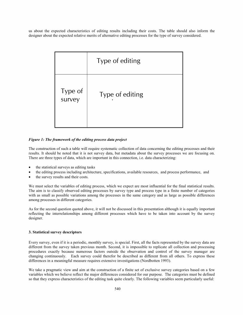
The answer to the first question can in principle be imagined retrieved from a table as illustrated in Figure 1 andrepresenting the framework of the editing process data project. When designing a new survey, or redesigning an oldone, we want to identify first the row of the table corresponding to which type the survey belongs, and second thecolumn corresponding to the editing process considered. The cell of the row and column intersection should inform

1 Preparation of this paper was supported by Statistics Sweden. The author is grateful to Mr. Leopold Granquist fora number of constructive comments. The views expressed are not, however, necessarily those of Statistics Sweden.

540

us about the expected characteristics of editing results including their costs. The table should also inform thedesigner about the expected relative merits of alternative editing processes for the type of survey considered.

Figure 1: The framework of the editing process data project

The construction of such a table will require systematic collection of data concerning the editing processes and theirresults. It should be noted that it is not survey data, but metadata about the survey processes we are focusing on.There are three types of data, which are important in this connection, i.e. data characterizing:

• the statistical surveys as editing tasks• the editing process including architecture, specifications, available resources, and process performance, and• the survey results and their costs.

We must select the variables of editing process, which we expect are most influential for the final statistical results.The aim is to classify observed editing processes by survey type and process type in a finite number of categorieswith as small as possible variations among the processes in the same category and as large as possible differencesamong processes in different categories.

As for the second question quoted above, it will not be discussed in this presentation although it is equally importantreflecting the interrelationships among different processes which have to be taken into account by the surveydesigner.

3. Statistical survey descriptors

Every survey, even if it is a periodic, monthly survey, is special. First, all the facts represented by the survey data aredifferent from the survey taken previous month. Second, it is impossible to replicate all collection and processingprocedures exactly because numerous factors outside the observation and control of the survey manager arechanging continuously. Each survey could therefor be described as different from all others. To express thesedifferences in a meaningful measure requires extensive investigations (Nordbotten 1993).

We take a pragmatic view and aim at the construction of a finite set of exclusive survey categories based on a fewvariables which we believe reflect the major differences considered for our purpose. The categories must be definedso that they express characteristics of the editing task quite clearly. The following variables seem particularly useful:

Type of editing

Type ofsurvey

Type of editingl

541

• The domain to which the survey belong• The periodicity of the survey• The number of records to be edited• The number of fields contained in each record.• The primary source from which the data is collected.• The data collection method.• The number of fields in other sources, which can be used as auxiliary data for editing.• The number of statistical estimates required from the survey.

In the SCB, most of this information is already recorded in its metadata system for the majority of surveys, and caneasily be retrieved for creation of survey categories and use as background variables in analysis of the editingprocess.

4. Editing processes descriptors

As already pointed out the aim of the editing activities is to detect and adjust for errors in the data in order toimprove the results of the survey. Assume ideal operational definitions for all survey variables exist. If these wereimplemented truthfully, no errors would exist in the data collected and processed, or in the statistics prepared. Thesehypothetical data are referred to as the target data of the survey.

In practical applications, the target data cannot usually be achieved because the ideal processes required would becost and time prohibitive for all units in the survey. Instead more convenient and practical procedures are establishedand executed. The result of these procedures is the raw data records.

Description of an editing process can be considered as divided into three parts, the editing architecture describingprinciples for the process, the editing specifications describing the numerical details of the architecture andresources available/used, and finally, the editing performance describing the execution of the editing process.

In the next paragraphs we shall explain the three main components of the editing metadata.

4.1 Architecture

If we could compare the target records with the raw records for each unit in a survey, the micro errors would beidentified. Similarly, if statistical aggregates based on the raw data could be compared with the correspondingaggregates of the target data, the macro errors would be discovered.

Obviously, the problem is that we do not know the target data records. The first component to be considered in anediting architecture is therefore a method to detect the raw data records that contain the most influential errors. Anumber of principles have been proposed and methods developed for this purpose. Most of the methods exploitsome kind of background knowledge about the units to define classes or ranges of erroneous or suspicious recordpatterns (UN/ECE 1997).

If a set of raw records has been identified as erroneous or suspicious, the next component of the architecture will beto find or develop a method for adjusting the records. Also for this task a repository of methods exists. The methodsrange from a complete re-collection and -processing of records for the units which were associated with the originalsuspicious raw records to using background information about the unit with a suspicious record, or similar units, toimpute new more probable values to replace suspicious values.

Combining existing and/or new methods produces a number of possible editing architectures. The architecture datawill therefore consist of descriptions of or references to individual methods applied and how they are combined inthe editing process.

542

4.2 Specification

To adapt an architecture to a specific application, numerical specification of a number of parameters, such as lowerand upper bounds for ratios of variables, determination of acceptable and suspicious combinations of categories fordiscrete variables, etc., are required.

The specification of the editing methods also implies available or allocated resources of different kinds, such ashuman inspectors, computer capacity and time. Data on specifications of the type indicated will play a central role inevaluation of editing processes because they in large will reflect the resources used in the application. A large part ofthe specifications has never been systematically recorded.

4.3 Performance

The part of the editing process, which has received most attention, is description of the process performance(Engström 1996; Engström 1997; Engström and Granquist 1999). Some typical variables, which can usually berecorded during the process, are shown in List 1. These basic variables give us important facts about the editingprocess.

N: Total number of observationsNC: Number of observations rejected as suspiciousNI: Number of imputed observationsX: Raw value sum for all observationsXC: Raw value sum for rejected observationsYI: Imputed value sum of rejected observationsY: Edited value sum of all observationsKC: Cost of editing controlsKI: Cost of imputations

List 1: Typical operational and cost variables

If the number of observations classified as suspicious in a periodic survey increased from one period to another, itcan, for example, be interpreted as an indication that the raw data have decreasing quality, or that the edit parametershave become out of date since they were established. On the other hand, if the editing procedure has a satisfactoryquality, it can also be regarded as indication of increased quality of the results, because more units are rejected forcareful inspection. A correct conclusion may require that several of the variables be studied simultaneously. As afirst step toward a better understanding of the editing process, the basic variables can be combined in different ways.List 2 gives examples of a few composite variables being used for monitoring and evaluating the editing process.

The reject frequency, FC, indicates the relative extent of the control work performed. This variable gives a measureof the workload a certain control method implies, and is used to tune the control criteria according to availableresources. In an experimental design stage, the reject frequency is used to compare and choose between alternativemethods.

The imputation effects on the rejected set of NC observations are the second group of variables. The imputefrequency, FI, indicate the relative number of observations which have their values changed during the process. FIshould obviously not be larger than FC. If the difference Fc - FI is significant, it may be an indication that therejection criteria are to narrow, or perhaps that more resources should be allocated to make the inspection andimputation of rejected observations more effective.

543

List 2: Some typical operational and cost ratios

The rejected value ratio, RC, measures the impact of the rejected values relative to the total value of all raw values.A small rejected value ratio may indicate that the suspicious values are an insignificant part of the total of values.Alternatively, the total of rejected values could be compared with the edited value sum of all observations. In bothcases, the indicator may hide large changes in opposite directions.

If the rejected value ratio is combined with a high FC, a review of the process may conclude that the resources spenton inspection of rejected values cannot be justified and are in fact better used for some other process. RC may showthat even though the FC is large, the RC may be small which may be another indication that the current editingprocedure is not well balanced.

The impute ratio, RI, indicates the overall effect of the editing and imputation on the raw observations. If RI is small,we may suspect that resources may be wasted on editing.

Costs per rejected unit, KC, and cost per imputed unit, KI, add up to the total editing cost per unit. The costs perproduct (item) have to be computed indicators based on a cost distribution scheme since only totals will be availablefrom the accounting system.

The process data are computed from both raw and edited micro data. The importance of preserving also the originalraw data has now become obvious and it should become usual practice that the files of raw and edited micro data arecarefully stored.

The process variables computed are often used independently of each other. The editing process can easily beevaluated differently depending on which variables are used. The purpose of the next section is to investigate howthe process can be described by a set of interrelated variables, which may give further knowledge about the nature ofthe editing process and a basis for improved future designs.

5. Statistical quality descriptors

Editing itself has no meaning in itself. It is the impact it may have on future statistical results, which counts. Wewill use the quality concept as a summary descriptor for a statistical product, and discuss this descriptor in moredetail in the next paragraphs.

Frequencies:FC =NC/N (Reject frequency)FI =NI/N (Impute frequency)

Ratios:RC =XC/X (Reject ratio) RI =YI/X (Impute ratio)

Per unit values:KC = KC/ N (Cost per rejected unit) KI = KI /N (Cost per imputed unit)

544

5.1 Quality and errors

The quality of a statistical product, is determined by a number of factors including product relevance(correspondence between the target concept and the concept required by a typical application), timeliness (the periodbetween the time of the observed events and the time at which the product was used), and accuracy (the deviationbetween the target size and the product size) (Depoutot 1998). Wider quality concepts, as used for example byStatistics Canada, include also accessibility, interpretability and coherence (Statistics Canada 1998). It should benoted that the quality as experienced by two or more users might be different because their needs may have differentrequirements. In this presentation, we consider mainly the accuracy dimension of quality.

The users want quality descriptors to decide if the supplied statistics are suitable for their needs, while the producersneed data on quality to select among alternative production strategies and to allocate resources for improving overallproduction performance. Quality can never be precisely described. One obvious reason is that the precise quality ofa statistical product presumes knowledge of the target size, and if we knew the target size there would be no need formeasuring the fact. Another reason is, as mentioned above, that the desired target concept may vary among theusers. The descriptor reflects the quality of some kind of average user. While a quality statement expressesuncertainty about a statistical product, uncertainty will also be a part of the quality measurement itself.

5.2 Measuring quality

So far, the statistical product quality has been discussed from an abstract perspective. To be useful, the abstractnotion of quality must be replaced by an operational variable, which can be measured and processed.

As already discussed, quality cannot be observed exactly, but it can, subject to a specified risk, be indicated by anupper bound for the deviation of the product size from the target size.

Consider the expression:

Pr (|Y’-Y|>D)=1-p

which implies that the risk that the product size Y’ deviates from its target size Y with more than D is (1-p). D is aquality metric even though it decreases by increasing quality and in fact is an error metric. Because Y is unknown,we must substitute D by an estimate D’ (Nordbotten 1998). Subject to certain assumptions, it can be demonstratedthat D’ = k (p)* var (Y') where the value of k is determined by the probability distribution of Y’ and a specified valueof p. Assuming that Y' has a normal distribution, k is easily available in statistical tables.

In order to compute the estimate D’, we need a small sample of individual records with edited as well as raw data toestimate the variance of Y'. If the raw records for these units can be re-submitted for an approximately ideal editingto obtain a third set of records containing individual target data, we can compute Y as well as D' for differentconfidence levels p. It can be shown that a smaller risk (1-p) is related to a larger D’ for the same product andsample.

Because D’ is itself subject to errors, the estimator may or may not provide satisfactory credibility. It is thereforeimportant to test the estimator empirically. In experiments with individual data for which both edited and target dataversions exist, statistical tests comparing estimate D’, and the target D, can be carried out (Nordbotten 1998;Nordbotten 2000; Weir 1997).

Manzari and Della Rocca distinguish between output oriented and input oriented approaches to evaluation of editingand imputation procedures (Manzari and Della Rocca 1999). In an output oriented approach they focus on the effectof the editing on resulting products, while in an input oriented approach they concentrate on the effect of the editingon the individual data items. The quality indicator D’ presented in here is a typical example of an output orientedapproach while the performance variables discussed in section 4, are examples of an input oriented approach toevaluating the editing procedures.

545

6. Analyzing editing data

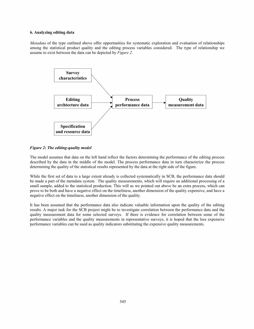
Metadata of the type outlined above offer opportunities for systematic exploration and evaluation of relationshipsamong the statistical product quality and the editing process variables considered. The type of relationship weassume to exist between the data can be depicted by Figure 2.

Figure 2: The editing-quality model

The model assumes that data on the left hand reflect the factors determining the performance of the editing processdescribed by the data in the middle of the model. The process performance data in turn characterize the processdetermining the quality of the statistical results represented by the data at the right side of the figure.

While the first set of data to a large extent already is collected systematically in SCB, the performance data shouldbe made a part of the metadata system. The quality measurements, which will require an additional processing of asmall sample, added to the statistical production. This will as we pointed out above be an extra process, which canprove to be both and have a negative effect on the timeliness, another dimension of the quality expensive, and have anegative effect on the timeliness, another dimension of the quality.

It has been assumed that the performance data also indicate valuable information upon the quality of the editingresults. A major task for the SCB project might be to investigate correlation between the performance data and thequality measurement data for some selected surveys. If there is evidence for correlation between some of theperformance variables and the quality measurements in representative surveys, it is hoped that the less expensiveperformance variables can be used as quality indicators substituting the expensive quality measurements.

Editingarchtecture data

Specificationand resource data

Processperformance data

Qualitymeasurement data

Surveycharacteristics

546

7. References

Depoutot, R. (1998), "Quality of International Statistics: Comparability and Coherence," Presented at theConference on Methodological Issues in Official Statistics, Stockholm.

Engström, P. (1996), "Monitoring the Editing Process," Presented at the UN/ECE Works Session on Statistical DataEditing, Voorburg.

Engström, P. (1997), "A Small Study on Using Editing Process Data for Evaluation of the European Structure ofEarnings Survey," Paper presented at the UN/ECE Work Session on Statistical Data Editing, Prague.

Engström, P. and Granquist, L. (1999), “Improving Quality by Modern Editing”, Presented at the UN/ECE WorkSession on Statistical Data Editing, Rome.

Granquist, L. (1996), “The New View on Editing," Presented at the UN/ECE Work Session on Statistical DataEditing, Voorburg.

Granquist, L. (1997a), “On the CBM-document: Edit Efficiently”, Presented at the UN/ECE Work Session onStatistical Data Editing, Prague.

Granquist, L (1997b), "An Overview of Methods of Evaluating Data Editing Procedures," Statistical Data Editing,Vol. 2, Methods and Techniques. Statistical Standards and Studies No 48. UN/ECE. pp. 112 122.

Jong, W.A.M. de (1996), "Designing a Complete Edit Strategy - Combining Techniques,” Presented at the UN/ECEWork Session on Statistical Data Editing, Voorburg.

Nordbotten, S. (1963), "Automatic Editing of Individual Statistical Observations," Statistical Standards and Studies.Handbook No. 2. United Nations, N.Y.

Nordbotten, S. (1993): "Statistical Meta-Knowledge and –Data," Presented at the Workshop on Statistical MetaData Systems, EEC Eurostat, Luxembourg, and published in Journal of Statistics, UN/ECE, Vol. 10, No.2, Geneva,pp. 101-112.

Nordbotten, S. (1998), "Estimating Population Proportions from Imputed Data," Computational Statistics & DataAnalysis, Vol. 27, pp. 291-309.

Nordbotten, S. (2000), "Evaluating Efficiency of Statistical Data Editing: General Framework," UN/ECE, Geneva.

Sundgren, B. (1991): “What Metainformation should Accompany Statistical Macrodata?” R&D Report, StatisticsSweden, Stockholm.

Sundgren, B. (1994): “Statistical Metadata and Metainformation Systems,” Statistics Sweden, Stockholm.

UN/ECE (1997), "Methods and Techniques," Statistical Standards and Studies No. 48. UN/ECE, Geneva.

Weir, P. (1997), "Data Editing and Performance Measures," Presented at the UN/ECE Works Session on StatisticalData Editing, Prague.

547

DESIGN OF INLIER AND OUTLIER EDITS FOR BUSINESS SURVEYS

David DesJardins and William E. WinklerWilliam E. Winkler, Rm. 3000-4, U.S. Bureau of the Census, Washington, DC 20233-9100 USA

david.l.desjardins@ccmail.census.gov, william.e.winkler@ccmail.census.gov

ABSTRACT

Establishment surveys can be challenging to edit. Some of the conventional editing methods have involved review of printoutsand subsequent correction of fields in records that are thought to be erroneous. A limitation of these conventional methods --even when well-designed -- is that they channel the reviewers in a manner that may not allow a number of the errors to be found. New software packages make it very straightforward to apply graphical based methods. The graphical methods can be appliedin an exploratory manner to discover nuances that conventional methods are likely to miss. Further, the graphical methods allowconfirmatory review of data to assure that corrections due to the editing process have worked well.

Keywords: Exploratory Data Analysis, graphics, industry profile and leverage plots, mixture

1. INTRODUCTION

This paper shows how a series of well-designed graphical methods can be developed and used to explore and findanomalies in the data. Most graphical methods allow detection of outliers in distributions that may be in error. Furthermore, these graphical methods can yield insight into situations in which more subtle distributional errors occur. New graphical packages are often very easy to use to locate and correct errors outliers in data. Cleveland (1993) hasprovided a variety of graphical methods. Granquist (1997) and Hogan (1995) have shown how to apply some of themethods to files of businesses.

An outlier is a data value that lies in the tail of the statistical distribution of a set of data values. The intuition is thatoutliers in the distribution of uncorrected (raw) data are more likely to be incorrect. Examples are data values that liein the tails of the distributions of ratios of two fields (ratio edits), weighted sums of fields (linear inequality edits), andMahalanobis distributions (multivariate normal) or outlying points to point clouds of graphs. An inlier is a data valuethat lies in the interior of a statistical distribution and is in error. Because inliers are difficult to distinguish from gooddata values they are sometimes difficult to find and correct. A simple example of an inlier might be a value in a recordreported in the wrong units, say degrees Fahrenheit instead of degrees Celsius.

Isolated inliers may not be a problem and may be almost impossible to distinguish from correct data. Sets of inliers ofmoderate size may seriously affect uses of microdata. In some situations, we can use graphical methods to discover thesesets of inliers. In other situations, we may use conventional methods for finding mixture distributions to locate and,possibly, correct the data. In more advanced situations, sets of inliers may arise when two or more administrative listsare linked and some of the identifying information is in error. If corrections are done, then we can use the graphicalmethods to confirm the plausibility of the changes.

In this paper, we provide an overview of the graphical methods. We show how they can be used to clean up data ordetermine that there are errors in data for which clean up methods need to be created. The outline of this paper is asfollows. In the second section, we cover how exploratory data analysis (EDA) methods can be used to detect errors andcorrect data. Although the methods are often quite straightforward to learn and apply, they often yield information aboutserious errors that have previously gone undetected. In the third section, we show how EDA methods can indicate theexistence of a large number of inliers. The inliers might arise as a mixture of two distributions. They might also arisewhen quantitative data from two administrative lists are linked (Scheuren and Winkler 1997). In some situations,conventional methods as described in the second section can be used for corrections. In other situations, new methodsare needed for creating data suitable for use in analyses. The graphical methods provide a check on the efficacy ofapplications and corrections. The final section consists of concluding remarks.

548

2. EDA GRAPHICS AND OUTLIER DETECTION

Conventional edit methods have often involved the development of if-then-else rules in computer software that delineaterecords that may need editing. These methods have typically been used in computer environments in which printoutswere created for analyst review. Review and correction of these data can be time-consuming. Errors may not be locatedbecause edit rules are inflexible or are not designed to detect certain classes of mistakes. Methods that are developedfor one survey may not be exactly appropriate on other surveys. Errors in data may vary as industries change. Updatedsets of questions may be asked.

Use of modern, graphical data software in an exploratory manner allows analysts to detect errors that cannot be detectedby inflexible editing rules. The software packages provide easy methods for updating databases as errors are corrected.Statistical agencies often do not know how easily the methods can be applied. They may not be aware of trainingcourses.

EDA methods allow analysts to discover errors in data. The fixed computer algorithms of conventional edit methodshave often missed unanticipated errors in the data. The fixed algorithms are blind in the sense that they cannot adaptto new situations. For instance, comparing variables and using ratios requires a very good understanding of the oftenunique/unpredictable relationships between each of the variables. These relationships can vary markedly for differentpoint cloud clusters associated/corresponding to companies in different industrial codes. The variation can be substantialbetween companies in different size ranges or when survey forms are re-designed. Time series variances such as businesscycles and periodic anomalies can affect the relationships. Basic relationships for data sets can also vary substantiallyover time as well. By using powerful graphics tools in combination with an individual trained in EDA methodology,these problems can be quickly identified and dealt with. In addition to producing outliers, these factors often hide inliers.

In this section, we show how EDA methods provide a Arevolution@ in data analysis in statistical agencies that have notsystematically used the methods. The section highlights key examples of where EDA has shown itself to be significantlybetter at data editing, in the analysis of data, and for identifying outliers and inliers. It is also often much better atdiscovering undetected flaws in traditional data analysis methodologies in data at statistical agencies.

Four key factors contribute to this Arevolution@ in data analysis and make the introduction of these EDA methods at thistime a momentous opportunity. First, these graphics software packages provide most analysts with the ability to generatehundreds of graphs in a matter of mere minutes. Generating such a large number of graphs would have taken weeks justa few years ago. Second, these interactive software packages often allow sophisticated graphical methods of lookingat the data and reviewing subcomponents of it. If the analysts believe the data are in error, then they can easilydiscover/correct it in an interactive manner using these point-and-click tools. Third, some versions of the software areinexpensive. Student versions of these PC software packages are often available for less than $100. Fourth, and mostimportant, individuals using these multi-purpose EDA techniques are not locked into custom designed software packagesand fixed ways of looking at the data. By using the above hardware and software tools, we (see particularly DesJardins1998) have developed new general-purpose graphical forms and special techniques that greatly enhance the speed andefficiency of data editing/analysis tasks. Analysts no longer spend time editing their data with fixed methods andcumbersome, boring, tabular printouts.

Graphs communicate across a wide area of expertise. A properly chosen graph can make some sophisticated statisticalconcepts clear to laymen. Statisticians can now more quickly/effectively explain to subject matter specialists thefundamental concepts behind these new graphical data analysis techniques. In this section, the graphs are cut and pastedfrom the outputs of graphics software such as SAS Insight and SAS JMP. SAS Insight is available as an addition to thebasic SAS package. SAS JMP is available for Macintosh and Windows PCs. A comprehensive SAS JMP-IN versionis available for only about $60 for students (with a 500+ page statistical data analysis manual). NOTE: Forconfidentiality reasons, all the examples used in this paper contain anonymized data or artificial data that are similar toreal data.

549

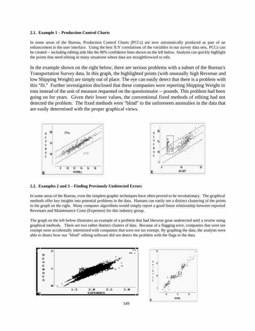
2.1. Example 1 – Production Control Charts

In some areas of the Bureau, Production Control Charts (PCCs) are now automatically produced as part of anenhancement to the user interface. Using the best X/Y correlations of the variables in our survey data sets, PCCs canbe created -- including editing aids like the 80% confidence lines shown on the left below. Analysts can quickly highlightthe points that need editing in many situations where data are straightforward to edit.

In the example shown on the right below, there are serious problems with a subset of the Bureau'sTransportation Survey data. In this graph, the highlighted points (with unusually high Revenue andlow Shipping Weight) are simply out of place. The eye can easily detect that there is a problem withthis Afit.@ Further investigation disclosed that these companies were reporting Shipping Weight intons instead of the unit of measure requested on the questionnaire -- pounds. This problem had beengoing on for years. Given their lower values, the conventional fixed methods of editing had notdetected the problem. The fixed methods were "blind" to the unforeseen anomalies in the data thatare easily determined with the proper graphical views.

2.2. Examples 2 and 3 – Finding Previously Undetected Errors

In some areas of the Bureau, even the simplest graphic techniques have often proved to be revolutionary. The graphicalmethods offer key insights into potential problems in the data. Humans can easily see a distinct clustering of the pointsin the graph on the right. Many computer algorithms would simply report a good linear relationship between reportedRevenues and Maintenance Costs (Expenses) for this industry group.

The graph on the left below illustrates an example of a problem that had likewise gone undetected until a review usinggraphical methods. There are two rather distinct clusters of data. Because of a flagging error, companies that were taxexempt were accidentally intermixed with companies that were not tax exempt. By graphing the data, the analysts wereable to detect how our "blind" editing software did not detect the problem with the flags in the data.

550

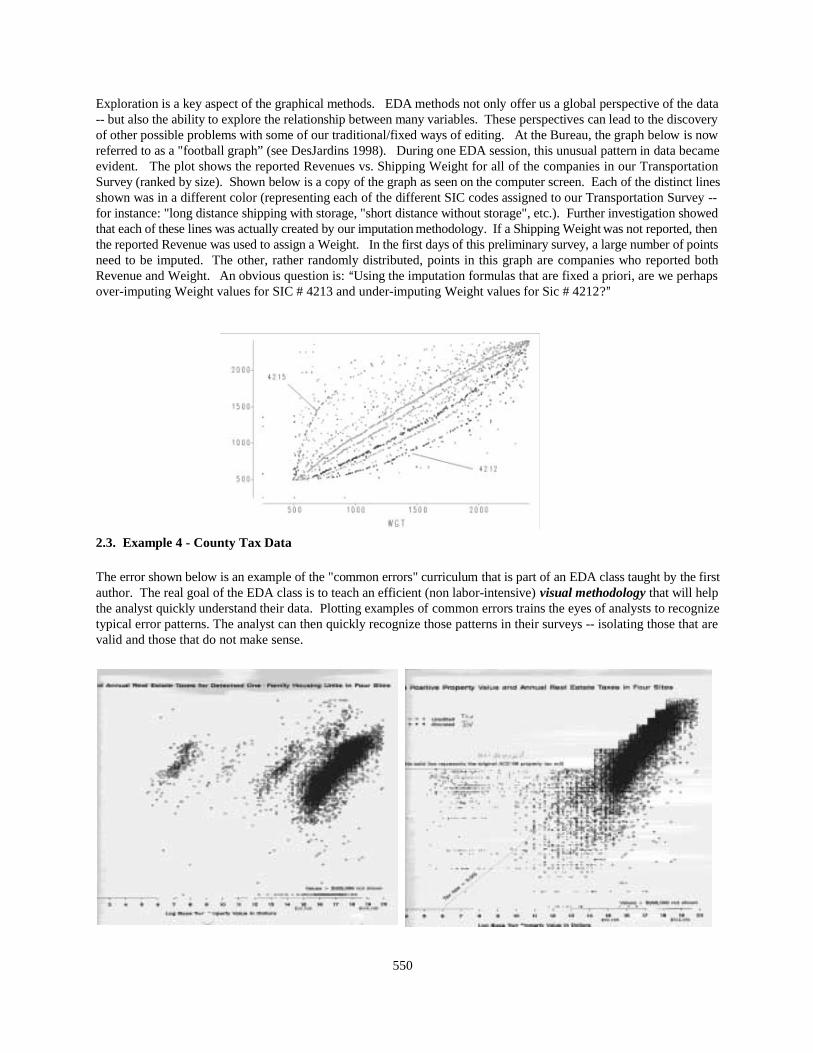
Exploration is a key aspect of the graphical methods. EDA methods not only offer us a global perspective of the data-- but also the ability to explore the relationship between many variables. These perspectives can lead to the discoveryof other possible problems with some of our traditional/fixed ways of editing. At the Bureau, the graph below is nowreferred to as a "football graph” (see DesJardins 1998). During one EDA session, this unusual pattern in data becameevident. The plot shows the reported Revenues vs. Shipping Weight for all of the companies in our TransportationSurvey (ranked by size). Shown below is a copy of the graph as seen on the computer screen. Each of the distinct linesshown was in a different color (representing each of the different SIC codes assigned to our Transportation Survey --for instance: "long distance shipping with storage, "short distance without storage", etc.). Further investigation showedthat each of these lines was actually created by our imputation methodology. If a Shipping Weight was not reported, thenthe reported Revenue was used to assign a Weight. In the first days of this preliminary survey, a large number of pointsneed to be imputed. The other, rather randomly distributed, points in this graph are companies who reported bothRevenue and Weight. An obvious question is: AUsing the imputation formulas that are fixed a priori, are we perhapsover-imputing Weight values for SIC # 4213 and under-imputing Weight values for Sic # 4212?@

2.3. Example 4 - County Tax Data

The error shown below is an example of the "common errors" curriculum that is part of an EDA class taught by the firstauthor. The real goal of the EDA class is to teach an efficient (non labor-intensive) visual methodology that will helpthe analyst quickly understand their data. Plotting examples of common errors trains the eyes of analysts to recognizetypical error patterns. The analyst can then quickly recognize those patterns in their surveys -- isolating those that arevalid and those that do not make sense.

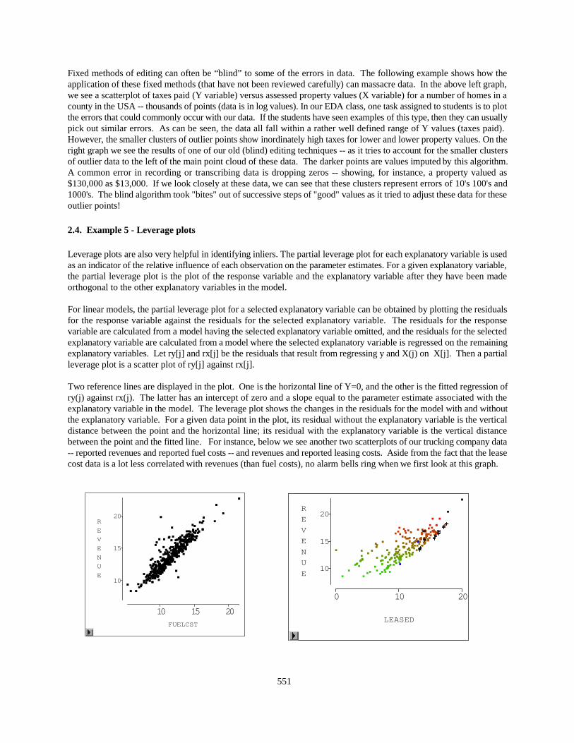
551

Fixed methods of editing can often be “blind” to some of the errors in data. The following example shows how theapplication of these fixed methods (that have not been reviewed carefully) can massacre data. In the above left graph,we see a scatterplot of taxes paid (Y variable) versus assessed property values (X variable) for a number of homes in acounty in the USA -- thousands of points (data is in log values). In our EDA class, one task assigned to students is to plotthe errors that could commonly occur with our data. If the students have seen examples of this type, then they can usuallypick out similar errors. As can be seen, the data all fall within a rather well defined range of Y values (taxes paid). However, the smaller clusters of outlier points show inordinately high taxes for lower and lower property values. On theright graph we see the results of one of our old (blind) editing techniques -- as it tries to account for the smaller clustersof outlier data to the left of the main point cloud of these data. The darker points are values imputed by this algorithm.A common error in recording or transcribing data is dropping zeros -- showing, for instance, a property valued as$130,000 as $13,000. If we look closely at these data, we can see that these clusters represent errors of 10's 100's and1000's. The blind algorithm took "bites" out of successive steps of "good" values as it tried to adjust these data for theseoutlier points!

2.4. Example 5 - Leverage plots

Leverage plots are also very helpful in identifying inliers. The partial leverage plot for each explanatory variable is usedas an indicator of the relative influence of each observation on the parameter estimates. For a given explanatory variable,the partial leverage plot is the plot of the response variable and the explanatory variable after they have been madeorthogonal to the other explanatory variables in the model.

For linear models, the partial leverage plot for a selected explanatory variable can be obtained by plotting the residualsfor the response variable against the residuals for the selected explanatory variable. The residuals for the responsevariable are calculated from a model having the selected explanatory variable omitted, and the residuals for the selectedexplanatory variable are calculated from a model where the selected explanatory variable is regressed on the remainingexplanatory variables. Let ry[j] and rx[j] be the residuals that result from regressing y and X(j) on X[j]. Then a partialleverage plot is a scatter plot of ry[j] against rx[j].

Two reference lines are displayed in the plot. One is the horizontal line of Y=0, and the other is the fitted regression ofry(j) against rx(j). The latter has an intercept of zero and a slope equal to the parameter estimate associated with theexplanatory variable in the model. The leverage plot shows the changes in the residuals for the model with and withoutthe explanatory variable. For a given data point in the plot, its residual without the explanatory variable is the verticaldistance between the point and the horizontal line; its residual with the explanatory variable is the vertical distancebetween the point and the fitted line. For instance, below we see another two scatterplots of our trucking company data-- reported revenues and reported fuel costs -- and revenues and reported leasing costs. Aside from the fact that the leasecost data is a lot less correlated with revenues (than fuel costs), no alarm bells ring when we first look at this graph.

0 10 20

LEASED

10

15

20R

E

V

E

N

U

E

10 15 20FUELCST

10

15

20R

E

V

E

N

U

E

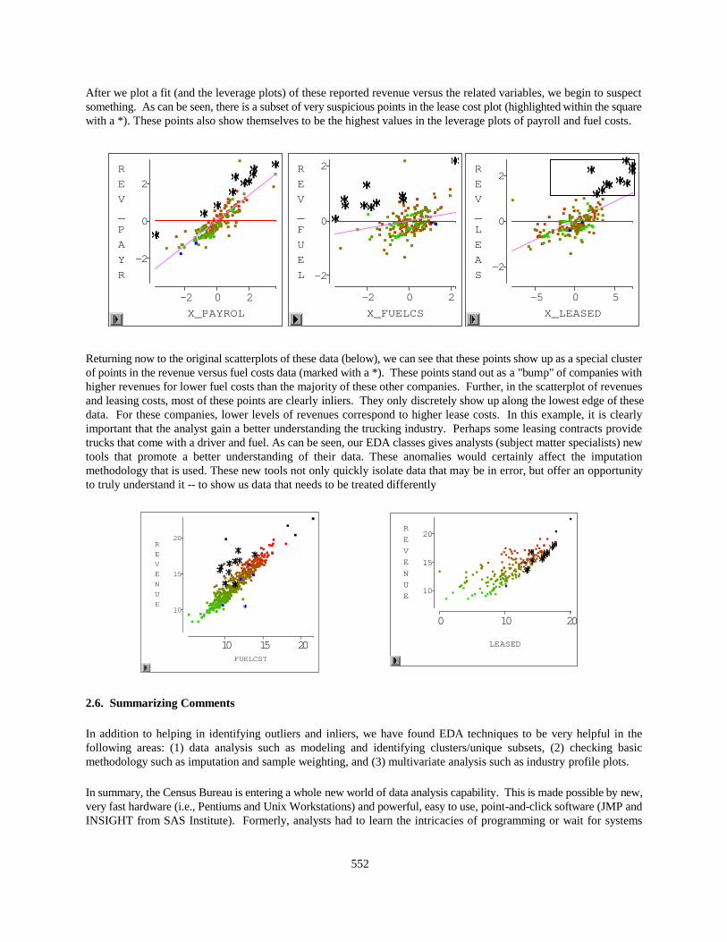
552

After we plot a fit (and the leverage plots) of these reported revenue versus the related variables, we begin to suspectsomething. As can be seen, there is a subset of very suspicious points in the lease cost plot (highlighted within the squarewith a *). These points also show themselves to be the highest values in the leverage plots of payroll and fuel costs.

Returning now to the original scatterplots of these data (below), we can see that these points show up as a special clusterof points in the revenue versus fuel costs data (marked with a *). These points stand out as a "bump" of companies withhigher revenues for lower fuel costs than the majority of these other companies. Further, in the scatterplot of revenuesand leasing costs, most of these points are clearly inliers. They only discretely show up along the lowest edge of thesedata. For these companies, lower levels of revenues correspond to higher lease costs. In this example, it is clearlyimportant that the analyst gain a better understanding the trucking industry. Perhaps some leasing contracts providetrucks that come with a driver and fuel. As can be seen, our EDA classes gives analysts (subject matter specialists) newtools that promote a better understanding of their data. These anomalies would certainly affect the imputationmethodology that is used. These new tools not only quickly isolate data that may be in error, but offer an opportunityto truly understand it -- to show us data that needs to be treated differently

2.6. Summarizing Comments

In addition to helping in identifying outliers and inliers, we have found EDA techniques to be very helpful in thefollowing areas: (1) data analysis such as modeling and identifying clusters/unique subsets, (2) checking basicmethodology such as imputation and sample weighting, and (3) multivariate analysis such as industry profile plots.

In summary, the Census Bureau is entering a whole new world of data analysis capability. This is made possible by new,very fast hardware (i.e., Pentiums and Unix Workstations) and powerful, easy to use, point-and-click software (JMP andINSIGHT from SAS Institute). Formerly, analysts had to learn the intricacies of programming or wait for systems

-2 0 2X_PAYROL

-2

0

2

R

E

V

_

P

A

Y

R

-2 0 2

X_FUELCS

-2

0

2R

E

V

_

F

U

E

L-2

0

2R

E

V

_

L

E

A

S

-5 0 5

X_LEASED

10 15 20FUELCST

10

15

20R

E

V

E

N

U

E

0 10 20

LEASED

10

15

20R

E

V

E

N

U

E

553

development efforts to produce custom software that they needed for their data analysis tasks. Instead, in conjunctionwith a quick, 40 hour, EDA course taught by the first author, analysts are being taught a variety of powerful EDAtechniques using an easy to learn (basically point-and-click) software. The design of this courseware is revolutionary intwo other ways as well. First, it stresses a multivariate analysis -- or all of the variables on the survey form -- allowingfor comparisons between variables in these data sets that, until now, had not been compared. The result is that we gaina real understanding of these data. Second, it is designed for subject matter specialists who have only a moderatestatistical background -- to give them key insights into their data.

3. INLIER DETECTION AND RESOLUTION

The previous section covered powerful EDA methods that can be easily applied by subject matter specialists who areanalyzing and correcting survey data. This section covers methods that use graphical methods and that may requireadditional analysis tools to be incorporated in software. Use of the methods in this section typically necessitates a deeperunderstanding of statistical models than the understanding of the previous section.

Users of statistical information are no longer content to use aggregate statistical data published in tables. They preferto use microdata because it allows them to perform policy and other statistical analyses that cannot be attempted whenonly aggregated data are available. By learning to run statistical packages or write elementary code to modify basicoutputs or inputs, these users have developed both simple and sophisticated models that give much greater insight thanthe insights obtained from using aggregate data. The direct analysis of databases has placed increased demands on dataproviders to eliminate outliers. It has sometimes yielded other improvements in the data or the systems providing thedata.

The first subsection describes how inliers and other errors can arise when groups of files are merged and the identifiersused for merging contain many errors. Such situations occur when groups of national and local health files and hospitalrecords are merged. The second subsection provides summarizing comments.

3.1. Using Edit/Imputation Modeling to Reduce Linkage Error

Multiple microdata files contain information that supports analyses that single files do not. For, instance, we might wantto use files of businesses that only have difficult-to-use name and address information in common. One file might containthe energy products consumed by the companies. The other file might contain the types and amounts of goods theyproduce. Another situation could arise with files on data that can be connected with appropriate edit/imputation models. For files of individuals, one file might have income data, another file might have information about health-relatedproducts, and a third file might have information about receipts of supplemental payments.

Appropriate microdata can support valid statistical analyses. Use of aggregate data does not allow evaluation ofcorrelations of data across files and accurate analyses on subdomains. We are interested in an edit/imputationmethodology for use on a file that is the merger of two or more files. The edit/imputation methodology can be used forcleaning data in the files and producing predicted quantitative values that can be used to improve matching. We assumethat the common data fields used for matching are not uniquely identifying and are subject to significant error. Thismakes linking (computer matching) of the correct corresponding microdata records very difficult. In a subset of thesesituations, each source file may contain noncommon quantitative that must be associated with an appropriate regressionmodel. If we have an appropriate methodology, then we may be able to edit/impute the microdata.

For simplicity, we consider the situation where records in a file are formed by merging (matching) two files (see alsoScheuren and Winkler 1997, Winkler 1997). The files are matched using very low quality name and address information. For each record, we assume that a matching score is available that summarizes the quality of the matching process. Forevaluation purposes, an indicator function tells whether each pair of records is a correct match or not. We do not makeuse of the (unobserved) indicator in developing methods. We do use it to confirm that the methods have workedreasonably well. Note that a similar scenario could also arise when records contain certain types of systematic error andan unobserved indicator function tells which records contain the systematic error. In the following example, name andaddress information is used in creating a file representing the merger of two other files. One file contains the y-variable

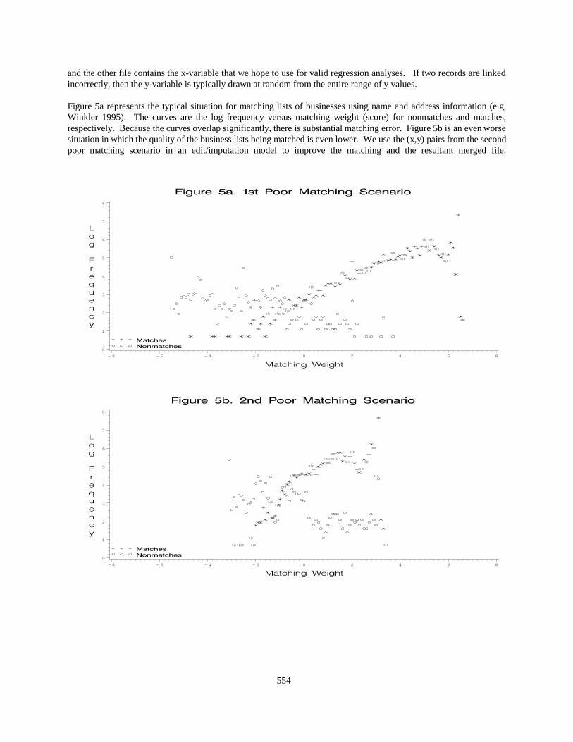
554

and the other file contains the x-variable that we hope to use for valid regression analyses. If two records are linkedincorrectly, then the y-variable is typically drawn at random from the entire range of y values.

Figure 5a represents the typical situation for matching lists of businesses using name and address information (e.g,Winkler 1995). The curves are the log frequency versus matching weight (score) for nonmatches and matches,respectively. Because the curves overlap significantly, there is substantial matching error. Figure 5b is an even worsesituation in which the quality of the business lists being matched is even lower. We use the (x,y) pairs from the secondpoor matching scenario in an edit/imputation model to improve the matching and the resultant merged file.

0

1

2

3

4

5

6

7

8

- 8 - 6 - 4 - 2 0 2 4 6 8

0

1

2

3

4

5

6

7

8

- 8 - 6 - 4 - 2 0 2 4 6 8

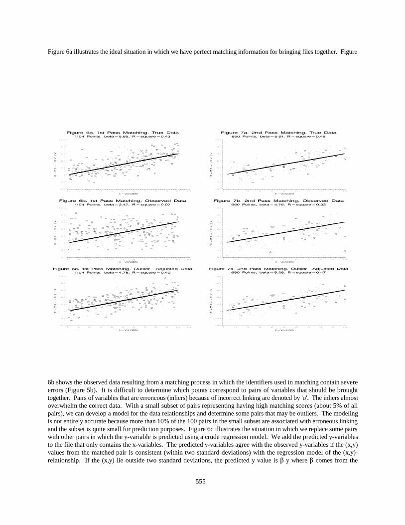
555

Figure 6a illustrates the ideal situation in which we have perfect matching information for bringing files together. Figure

6b shows the observed data resulting from a matching process in which the identifiers used in matching contain severeerrors (Figure 5b). It is difficult to determine which points correspond to pairs of variables that should be broughttogether. Pairs of variables that are erroneous (inliers) because of incorrect linking are denoted by 'o'. The inliers almostoverwhelm the correct data. With a small subset of pairs representing having high matching scores (about 5% of allpairs), we can develop a model for the data relationships and determine some pairs that may be outliers. The modelingis not entirely accurate because more than 10% of the 100 pairs in the small subset are associated with erroneous linkingand the subset is quite small for prediction purposes. Figure 6c illustrates the situation in which we replace some pairswith other pairs in which the y-variable is predicted using a crude regression model. We add the predicted y-variablesto the file that only contains the x-variables. The predicted y-variables agree with the observed y-variables if the (x,y)values from the matched pair is consistent (within two standard deviations) with the regression model of the (x,y)-relationship. If the (x,y) lie outside two standard deviations, the predicted y value is $ y where $ comes from the

- 4 0 0

- 2 0 0

0

2 0 0

4 0 0

6 0 0

8 0 0

1 0 0 0

0 1 0 2 0 3 0 4 0 5 0 6 0 7 0 8 0 9 0 1 0 0 1 1 0

T

T

TT

T

T

TT

T

T

T

T

T

TT

T

TT

T

T

T

T

T

T

T

T

T

T

TT

T

T

TT

T

T

T

T

T

T

T

T

T

T

T

T

T

T

T

T

T

T

T

T

T

T

T

T

TT

T

T T

TT

T

T

T

T

T

T

T

T

T

T

T

T

T

T

T

T

T

T

T

TT

T

T

T

T

T

TT

T

T

TT

T

T

T

T

T

TT

- 4 0 0

- 2 0 0

0

2 0 0

4 0 0

6 0 0

8 0 0

1 0 0 0

0 1 0 2 0 3 0 4 0 5 0 6 0 7 0 8 0 9 0 1 0 0

T

T

T

TT

T

T

T

T

T

T

T

T

T

T

T

T

T

T

T

T

T

T

T

T

T

T

T

T

T

T

T

T

T

T

T

T

T

T

T

T

T

T

T

T

T

T

T

T

T

T

T

T T

T

T

TT

T

T

T

T

T

T

T

T

T T

T

T

T

T

T

T

T

T

T

T

T

TT

T

TT

T

T

T

T

T

T

T

T

T

T

T

T

T

T

T

TT

TT

T

T

T

T

T

T

- 4 0 0

- 2 0 0

0

2 0 0

4 0 0

6 0 0

8 0 0

1 0 0 0

0 1 0 2 0 3 0 4 0 5 0 6 0 7 0 8 0 9 0 1 0 0 1 1 0

T

T

TT

T

T

TT

T

T

T

T

T

TT

T

TT

T

T

T

T

T

T

T

T

T

T

TT

T

T

TT

T

T

T

T

T

T

T

T

T

T

T

T

T

T

T

T

T

T

T

T

T

T

T

T

TT

T

T T

TT

T

T

T

T

T

T

T

T

T

T

T

T

T

T

T

T

T

T

T

TT

T

T

T

T

T

TT

T

T

TT

T

T

T

T

T

TT

- 4 0 0

- 2 0 0

0

2 0 0

4 0 0

6 0 0

8 0 0

1 0 0 0

0 1 0 2 0 3 0 4 0 5 0 6 0 7 0 8 0 9 0 1 0 0

T

T

T

TT

T

T

T

T

T

T

T

T

T

T

T

T

T

T

T

T

T

T

T

T

T

T

T

T

T

T

T

T

T

T

T

T

T

T

T

T

T

T

T

T

T

T

T

T

T

T

T

T T

T

T

TT

T

T

T

T

T

T

T

T

T T

T

T

T

T

T

T

T

T

T

T

T

TT

T

TT

T

T

T

T

T

T

T

T

T

T

T

T

T

T

T

TT

TT

T

T

T

T

T

T

- 4 0 0

- 2 0 0

0

2 0 0

4 0 0

6 0 0

8 0 0

1 0 0 0

0 1 0 2 0 3 0 4 0 5 0 6 0 7 0 8 0 9 0 1 0 0 1 1 0

T

T

TT

T

T

TT

T

T

T

T

T

TT

T

TT

T

TT

T

T

T

T

T

T

T

TT

T

T

TT

T

T

T

T

T

T

T

T

T

TT

T

T

T

T

T

T

T

T

T

T

T

T

T

TT

T

T T

TT

T

T

T

T

T

T

T

T

T

T

T

T

T

T

T

T

T

T

T

TT

T

T

T

T

T

T

TT

T

T

TT

T

T

T

T

T

T

T

- 4 0 0

- 2 0 0

0

2 0 0

4 0 0

6 0 0

8 0 0

1 0 0 0

0 1 0 2 0 3 0 4 0 5 0 6 0 7 0 8 0 9 0 1 0 0

T

T

T

TT

T

T

T

T

T

T

T

T

T

T

T

T

T

T

T

T

T

T

T

T

T

T

T

T

T

TT

T

T

T

T

T

T

T

T

T

T

T

T

T

T

T

T

T

T

T

T

T T

T

T

TT

T

T

T

T

T

T

T

T

T T

T

T

T

T

T

T

T

T

T

T

T

TT

T

TT

T

T

T

T

T

T

T

T

T

T

T

T

T

T

T

TT

TT

T

T

T

T

T

T

556

conjectured regression relationship. This yields an additional matching variable that we use to improve matching duringa second matching pass.

Figure 7a illustrates the true situation among the pairs if we had perfect matching information. Figure 7b shows that thevariables brought together during the second matching pass are more closely related. The reason that the plot in the right-hand column (Figure 7b) contains fewer points is that the predicted y-variables improve linking sufficiently tosubstantially reduce erroneous links (inliers). Finally, Figure 7c shows the result of some final modeling in whichoutliers in the merged file from the second matching pass are removed.

3.3. Summarizing Comments

To deal with inliers in most situations, we convert them to outliers using additional information that may be availablein the files being edited (see e.g., Winkler 1997). Only in the example of this section, administrative lists-analyticlinking, do we need to perform more work to create additional information that allows us to improve the data review anderror correction process. The analysis affects the updating of the edit/imputation process that produces the microdatafor general use.

4. CONCLUDING REMARKS

The ability of the eye-mind combination to discern subtle and complicated relationships during review of graphs has longbeen known (see e.g., Cleveland 1993). This paper has demonstrated that is it possible to use new, powerful, user-friendly graphical software to explore and correct data. Through his EDA/Graphics course, the first author has beenparticularly effective in moving the ideas in to day-to-day practice. The use of these EDA/Graphics techniques is alsonow a part of mainstream statistical methods for exploring and reviewing complicated statistical models.

1/ This paper reports the results of research and analysis undertaken by Census Bureau staff. It has undergone a Census Bureaureview more limited in scope than that given to official Census Bureau publications. This report is released to inform interestedparties of research and to encourage discussion.

5. REFERENCES

Cleveland, William (1993), Visualizing Data, Hobart Press: Summit, NJDesJardins, David (1998), “A New Graphical Techniques for the Analysis of Census Data”, Statistics Canada

Conference Proceedings.Granquist, L. (1997), “Macro-Editing - The Aggregate Method,” Statistical Data Editing, UN Conference of

European Statisticians Statistical Standards and Studies, Geneva (Switzerland).Hogan, Howard (1995), “How Exploratory Data Analysis is Improving the Way We Collect Business Statistics,”

American Statistical Association, Proceedings of the Section on Survey Research Methods, pp. 102-107.Scheuren, F. and Winkler, W. E. (1997), “Regression Analysis of Data Files that are Computer Matched, II,”

Survey Methodology, 23, pp. 157-165.Winkler, W. E. (1995), “Matching and Record Linkage,” in B. G. Cox et al. (ed.) Business Survey Methods, New

York: J. Wiley, pp. 355-384.Winkler, W. E. (1997), “Problems with Inliers,” paper presented at the European Conference of Statisticians,

October 14-17, 1997, Prague, Czech Republic.

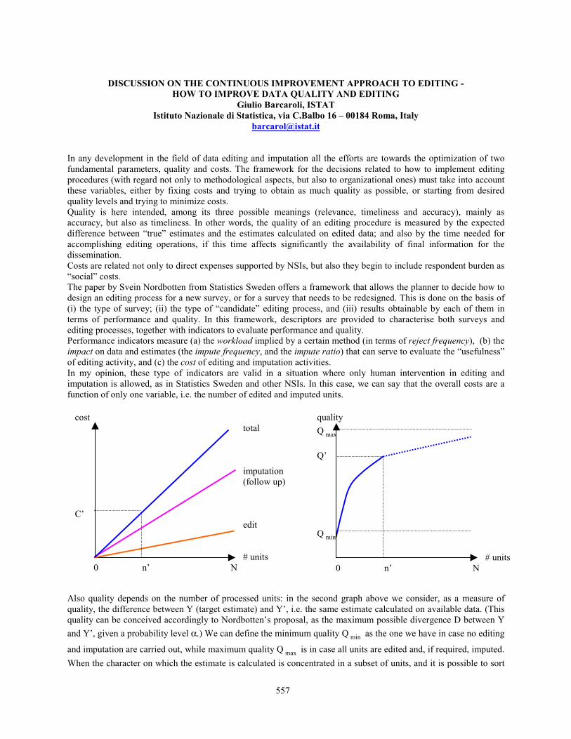
557

DISCUSSION ON THE CONTINUOUS IMPROVEMENT APPROACH TO EDITING -HOW TO IMPROVE DATA QUALITY AND EDITING

Giulio Barcaroli, ISTATIstituto Nazionale di Statistica, via C.Balbo 16 – 00184 Roma, Italy

barcarol@istat.it

In any development in the field of data editing and imputation all the efforts are towards the optimization of twofundamental parameters, quality and costs. The framework for the decisions related to how to implement editingprocedures (with regard not only to methodological aspects, but also to organizational ones) must take into accountthese variables, either by fixing costs and trying to obtain as much quality as possible, or starting from desiredquality levels and trying to minimize costs.Quality is here intended, among its three possible meanings (relevance, timeliness and accuracy), mainly asaccuracy, but also as timeliness. In other words, the quality of an editing procedure is measured by the expecteddifference between “true” estimates and the estimates calculated on edited data; and also by the time needed foraccomplishing editing operations, if this time affects significantly the availability of final information for thedissemination.Costs are related not only to direct expenses supported by NSIs, but also they begin to include respondent burden as“social” costs.The paper by Svein Nordbotten from Statistics Sweden offers a framework that allows the planner to decide how todesign an editing process for a new survey, or for a survey that needs to be redesigned. This is done on the basis of(i) the type of survey; (ii) the type of “candidate” editing process, and (iii) results obtainable by each of them interms of performance and quality. In this framework, descriptors are provided to characterise both surveys andediting processes, together with indicators to evaluate performance and quality.Performance indicators measure (a) the workload implied by a certain method (in terms of reject frequency), (b) theimpact on data and estimates (the impute frequency, and the impute ratio) that can serve to evaluate the “usefulness”of editing activity, and (c) the cost of editing and imputation activities.In my opinion, these type of indicators are valid in a situation where only human intervention in editing andimputation is allowed, as in Statistics Sweden and other NSIs. In this case, we can say that the overall costs are afunction of only one variable, i.e. the number of edited and imputed units.

Also quality depends on the number of processed units: in the second graph above we consider, as a measure ofquality, the difference between Y (target estimate) and Y’, i.e. the same estimate calculated on available data. (Thisquality can be conceived accordingly to Nordbotten’s proposal, as the maximum possible divergence D between Yand Y’, given a probability level α.) We can define the minimum quality Q min as the one we have in case no editing

and imputation are carried out, while maximum quality Q max is in case all units are edited and, if required, imputed.When the character on which the estimate is calculated is concentrated in a subset of units, and it is possible to sort

costtotal

imputation(follow up)

C’edit

# units 0 n’ N

qualityQ max

Q’

Q min

# units 0 n’ N

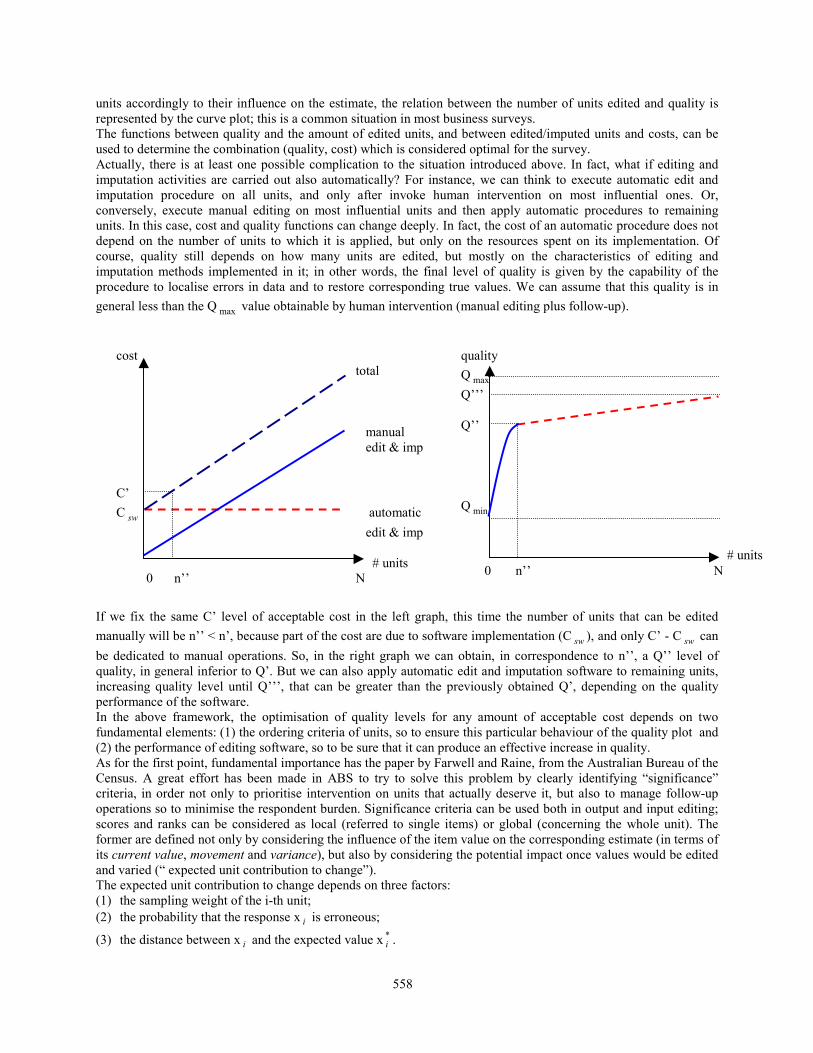
558

units accordingly to their influence on the estimate, the relation between the number of units edited and quality isrepresented by the curve plot; this is a common situation in most business surveys.The functions between quality and the amount of edited units, and between edited/imputed units and costs, can beused to determine the combination (quality, cost) which is considered optimal for the survey.Actually, there is at least one possible complication to the situation introduced above. In fact, what if editing andimputation activities are carried out also automatically? For instance, we can think to execute automatic edit andimputation procedure on all units, and only after invoke human intervention on most influential ones. Or,conversely, execute manual editing on most influential units and then apply automatic procedures to remainingunits. In this case, cost and quality functions can change deeply. In fact, the cost of an automatic procedure does notdepend on the number of units to which it is applied, but only on the resources spent on its implementation. Ofcourse, quality still depends on how many units are edited, but mostly on the characteristics of editing andimputation methods implemented in it; in other words, the final level of quality is given by the capability of theprocedure to localise errors in data and to restore corresponding true values. We can assume that this quality is ingeneral less than the Q max value obtainable by human intervention (manual editing plus follow-up).

If we fix the same C’ level of acceptable cost in the left graph, this time the number of units that can be editedmanually will be n’’ < n’, because part of the cost are due to software implementation (C sw ), and only C’ - C sw canbe dedicated to manual operations. So, in the right graph we can obtain, in correspondence to n’’, a Q’’ level ofquality, in general inferior to Q’. But we can also apply automatic edit and imputation software to remaining units,increasing quality level until Q’’’, that can be greater than the previously obtained Q’, depending on the qualityperformance of the software.In the above framework, the optimisation of quality levels for any amount of acceptable cost depends on twofundamental elements: (1) the ordering criteria of units, so to ensure this particular behaviour of the quality plot and(2) the performance of editing software, so to be sure that it can produce an effective increase in quality.As for the first point, fundamental importance has the paper by Farwell and Raine, from the Australian Bureau of theCensus. A great effort has been made in ABS to try to solve this problem by clearly identifying “significance”criteria, in order not only to prioritise intervention on units that actually deserve it, but also to manage follow-upoperations so to minimise the respondent burden. Significance criteria can be used both in output and input editing;scores and ranks can be considered as local (referred to single items) or global (concerning the whole unit). Theformer are defined not only by considering the influence of the item value on the corresponding estimate (in terms ofits current value, movement and variance), but also by considering the potential impact once values would be editedand varied (“ expected unit contribution to change”).The expected unit contribution to change depends on three factors:(1) the sampling weight of the i-th unit;(2) the probability that the response x i is erroneous;

(3) the distance between x i and the expected value x *i .

qualityQ max

Q’’’

Q’’

Q min

# units 0 n’’ N

costtotal

manual edit & imp

C’C sw automatic

edit & imp

# units 0 n’’ N

559

On the basis of the scores, it is possible:� to minimise costs on the basis of a desired limit to the bias, or� the inverse: to minimise bias on the basis of a fixed level of costs.Two main questions could be raised:A. how to measure the probability of error for each item x i ?

B. how to find the expected value x *i ?

The authors suggest to define error probabilities at unit level (higher for new units), or to set them always equal to 1.Moreover, they propose to use a system to impute likely responses, independent of response rates.My suggestion is: for both tasks, the most advanced methods for error localisation and data imputation, embedded ingeneralised software, could be used. In particular, Fellegi-Holt algorithms for error localisation ensure that theestimation of error probabilities for each item, given a set of edit rules, is optimised.Scores and ranks can be considered as local (referred to single items) or global (concerning the whole unit).The way the latter is defined is fundamental, as there can be conflicts between call-back priorities depending ondifferent local scores (a unit might be followed up for its influence on a particular estimate, but not for another).ABS’s proposal is to standardise local scores and then to combine them by assigning weights reflecting expertsassessment of their relative importance. The authors warn that no clear guidelines do exist to this regard. Actually,whenever you assign weights in computing a total score from single ones, on subjective basis, you risk to privilegere-contact of units that deserve it less than others do.In any case, an important and positive element that is taken into account in ABS is the consideration of therespondent burden as a social cost to be minimised, by integrating editing and respondents re-contact: a globalrespondent rank is computed by combining item scores, and on the basis of this rank any respondent is followed uponly once, rather than many times depending on the sequence of cyclic processing that characterises a traditionalediting system.Another problem in selective editing is that we privilege outliers detection. In doing so, we tend to introducedistortions in data, as in general data imputations produce a decrease in the total sum of a given character. To besymmetric, we should also detect inliers, i.e. units whose values lie inside an acceptance region, but nevertheless areerrors. The paper by David DesJardins and William Winkler, from the U.S. Bureau of the Census, containsproposals for detecting both outliers and inliers.As for inliers, the basic idea is to convert them into outliers by using additional information contained in files beingedited, by considering historical data, and by linking auxiliary information from other files. Exploratory DataAnalysis and graphical tools that enable human experts to detect and correct errors in distribution are proposed.Actually, the recent availability of powerful and not expensive software makes possible to analyse data, in a non-structured way, directly by subject matter experts, with no need of programming. The basic assumption is that inanalysing graph distributions, humans can recognise patterns (in particular clusters of units whose behaviour isdifferent from the others), that are not easily detectable by computer programs.This is true, but some objections to this approach can be raised. In principle, it is certain that human intelligence is(still) superior to the artificial one in pattern recognition; but to carry out all editing and imputation activities in a“creative” way as illustrated in the paper, could make it difficult to ensure some of the basic requirements such astransparency and reproducibility of the process. Human experts may react differently to similar situations (and thesame expert can behave differently in different occurrences of the survey). Perhaps if detection of outliers (andinliers) is left each time to the intuition of the individuals, too much undesired variability is introduced in theprocess.My opinion is that the use of such techniques can be very useful in a phase of design and implementation of editingand imputation rules. Let us suppose that we need to implement an automatic procedure, based for instance onSPEER software; the process of definition of ratio edits can exploit EDA and graphic tools in order to determinepairs of variables and lower and upper limits, but also the subpopulations for which the defined sets of edits arevalid. Furthermore, these techniques can be extremely valid to test and tune edits, and to find any particular new edituseful e.g. for inliers detection. In other words, it is proper to use creative tools in phases where creativity plays afundamental role, while in current editing operations it would be better to have a stable set of rules well defined andprecisely documented.

560