hybrid hydrologic modeling - pdfs.semanticscholar.org · hybrid hydrologic modeling 333 exhibit...

331

AuTHORS

Pierre Y. Julien is a professor of civil and environmental engineering at Colorado State University. He formerly served as an associate dean for International Research and Development. His research interest includes river mechanics, sediment transport, hydraulics, and hydrologic modeling. Dr. Julien has pub-lished extensively in water resources literature including two books and 20 lecture manuals and book chapters. He was an editor of the ASCE Journal of Hydraulic Engineering and received several awards including the H. A. Einstein Award for his contributions to sediment transport.

James S. Halgren is a water resources engineer with Riverside Technology, inc., consulting in areas of engineering modeling and programming. Dr. Halgren earned BS and MS degrees in civil engineering from Brigham Young University and received a PhD in civil engineering from Colorado State University in 2012. Dr. Halgren has presented lectures, conferences talks, and webinars on a number of his research and consulting projects, and he is an expert in geographic information systems (GIS), data analysis, and visualization.

17Hybrid Hydrologic

Modeling

17.1 Introduction to Hybrid Modeling ..................................................332Lumped vs. Distributed • Empirical, Conceptual, or Physical • Hybrid Modeling Concept

17.2 Modeling with TREX and SMA .....................................................333TREX • SAC-SMA

17.3 TREX-SMA: Model Processes and Algorithms ...........................334Rainfall and Interception • Soil Infiltration • Depression Storage • Overland and Channel Flow Routing • Soil Moisture Accounting in the Upper Zone • Soil Moisture Accounting in the Lower Zone

17.4 Hybrid Modeling Application at California Gulch .....................341Location and Site Description • Elevation and Topography • Land Use • Soil Type • Temperature • Evapotranspiration • Precipitation • Stream Flow • Hybrid Model Parameters

17.5 TREX-SMA Results and Discussion ............................................. 344Multi-Event Simulation Hydrographs • Overall Statistical Performance • Sources of Uncertainty • Advances in Model Visualization • Results Displayed with KML

17.6 Summary and Conclusions .............................................................350References ......................................................................................................350

Pierre Y. JulienColorado State University

James S. HalgrenRiverside Technology Inc.

© 2014 by Taylor & Francis Group, LLC

332 Handbook of Engineering Hydrology

17.1 Introduction to Hybrid Modeling

Systems of classification for different watershed models arise from differences in the way the hydrologic processes are represented [22].

17.1.1 Lumped vs. Distributed

One of the most common systems of hydrologic model classification is lumped vs. distributed. According to Abbot and Refsgaard [1], a lumped model is a model where the watershed is regarded as one unit and variables and parameters in the model represent average or effective values for the entire drainage area. On the other hand, a distributed model takes into account the spatial differences in all variables and parameters.

17.1.2 empirical, conceptual, or Physical

Physically based models represent flow using equations derived from the equations of conservation of mass, momentum, and energy. They internally use variables and parameters that directly represent physically measurable quantities in the field [11,12,23,45,47].

Conceptual models, by comparison, operate on parameters that represent a conceptualization of hydrologic processes. Aral and Gunduz [5] suggest that all lumped models are conceptual and non-physical, asserting that they contain no connection to physical processes except through a black-box empirical function.

17.1.3 Hybrid Modeling concept

Hybrid models can overcome the problems caused by dissimilarities in temporal and spatial scales of flow processes in the channel, overland plane, and subsurface. Aral and Gunduz [4] introduced the idea of a “hybrid modeling concept” in order to “resolve some of the problems associated with the fully phys-ics-based representation of all subsystem processes of a watershed while providing a much better and sophisticated interpretation that can be provided by an empirically based lumped parameter model.” For watershed modeling, “the small-scale requirements of overland and unsaturated zone flow domains

Preface

This chapter explores a new hybrid approach to hydrologic modeling. Hybrid modeling combines distributed surface runoff modeling with a lumped-parameter rendering of infiltration and sub-surface flow. The hybrid model TREX-SMA combines the Sacramento Soil Moisture Accounting (SAC-SMA) model with the TREX surface hydrology model. The capabilities of hybrid modeling are demonstrated with an application to the 30 km2 California Gulch watershed, near Leadville, Colorado. The results of a 50-day simulation are presented for comparisons with and without the hybrid model component SMA. Surface runoff parameters were obtained from a prior calibration of TREX, and the SMA soil moisture parameters were determined from a priori estimates used by the Arkansas Basin River Forecast Center (ABRFC) of the National Weather Service (NWS). The hybrid simulation results from TREX-SMA show improvement relative to results from the unmodified TREX model. Model results such as surface and channel water depth are processed with Geographic Resources Analysis Support System (GRASS) GIS and Keyhole Markup Language (KML) scripts to create 2.5-D, browsable animations overlaid on a Google Earth™ terrain.


Dow

nloa

ded

by [

Col

orad

o St

ate

Uni

vers

ity L

ibra

ries

], [

Pier

re J

ulie

n] a

t 08:

46 1

3 Ju

ne 2

014

Hybrid Hydrologic Modeling 333

exhibit severe limitations on efforts of fully integrating the system. Consequently, a hybrid modeling approach is more suitable in which distributed- and lumped-parameter models are essentially linked and blended to obtain a semi-distributed watershed model” [5].

“Semi-distributed” as used here indicates that a portion of the spatial or temporal domain is distrib-uted while the rest is lumped, hence “semi-distributed.” Kirchner [24] uses a similar line of reasoning to propose hybrid “gray box” models to allow some latitude for unexpected physical processes.

TREX and SAC-SMA differ in nearly all of the systems of classification: one is lumped and the other distributed; one is empirical and conceptual and the other is physically based. With these differences, the combination of these models can create a powerful hybrid.

This chapter illustrates the capabilities of hybrid hydrologic models. The example of TREX-SMA applications at California Gulch, Colorado, demonstrates the hybrid modeling capabilities.

17.2 Modeling with TreX and SMa

The main concept of hybrid modeling stems from the possible combination of the distributed surface-water modeling capabilities of TREX with the SAC-SMA techniques for soil moisture volumes and return flow from the subsurface.

The TREX surface runoff model was developed at Colorado State University, and the Sacramento Soil Moisture Accounting (SAC-SMA) model is well known from the National Weather Service (NWS). Each model has strengths that contribute to the hybrid, and each also has limitations, some of which are overcome with the hybrid approach.

17.2.1 TreX

The TREX model is based on the distributed surface hydrology model CASC2D developed at CSU [21,42]. Johnson [18] and Rojas-Sánchez [39] added a sediment transport algorithm, and the code was renamed CASC2D-SED [19,40,41]. Velleux [49] developed a contaminant transport algorithm with capability to model multiphase transport and fate of metals. The new code, now called TREX, was fully tested for the transport of Zn, Cu, and Cd from mining areas at California Gulch, Colorado [50,51]. The current TREX code is available on the web at www.engr.colostate.edu/trex.

17.2.2 Sac-SMa

The SAC-SMA model is part of the National Weather Service River Forecast System (NWSRFS), which is considered the standard in flood forecasting models for the United States [6,45]. SAC-SMA, together with simple routing models, provides a primary method for channel flow forecasting in the NWSRFS. The SAC-SMA model conceptualizes the watershed as an abstracted soil column divided vertically into two storage zones that are filled and emptied to simulate infiltration, percolation, baseflow, and inter-flow through the watershed. The upper and lower zones represent the infiltration capacity of shallow soils and the underlying aquifer, respectively.

Runoff is computed as the net excess volume remaining from precipitation after interception, and infiltration have been satisfied. Rates of infiltration and water holding capacities of the zones are rep-resented with conceptual parameters that, while not directly physical, correspond closely to physical values such as void space ratio and saturated hydraulic conductivities [6].

The conceptualization of finite volumes filling, draining, and spilling like a collection of intercon-nected buckets gives rise to the SAC-SMA model’s designation as a “bucket” model. Although not physi-cally based, the Sacramento model parameters can be estimated a priori using the assumption that plant extractable soil moisture is related to tension water and that free water storages relate to gravitational soil water [27]. Using soil properties defined in the Soil Survey Geographic (SSURGO) database and


Dow

nloa

ded

by [

Col

orad

o St

ate

Uni

vers

ity L

ibra

ries

], [

Pier

re J

ulie

n] a

t 08:

46 1

3 Ju

ne 2

014

http://www.engr.colostate.edu/trex


based on calibration experience, Anderson et al. [3] developed a range of acceptable values for 11 of the SAC-SMA parameters. Research by the NWS during recent years has focused on producing estimates of the SAC-SMA parameter values from known soil properties and remotely sensed data. These a priori estimates of the model parameters allow for uncalibrated simulation of watershed scale rainfall–runoff response with distributed versions of the SAC-SMA model [3,25,26,46].

17.3 TreX-SMa: Model Processes and algorithms

The TREX-SMA hybrid model has three primary layers: the TREX surface, the SAC-SMA upper zone, and the SAC-SMA lower zone. The hybrid model essentially preserves the raster-based distributed nature of the TREX model for the simulation of surface processes as well as the lumped and conceptual nature of soil moisture accounting with SMA. The links between the two models are provided from the following: (1) the infiltration from TREX is input to the SMA upper zone and (2) the SMA returns subsurface flow as point sources to the TREX surface flow algorithm.

More specifically, precipitation excess is calculated at each pixel and routed as 2-D surface runoff across the surface until it is conveyed as 1-D channel flow. The infiltration rates are removed from the surface domain and collectively lumped as input to the soil moisture accounting procedure of the SMA upper zone. Within the soil moisture accounting procedure, the volume (or depth) of water in the soil column is divided into two components: bound water and free-flowing water in both the upper zone and the lower zone. The free-flowing water replenishes the bound water zones when the latter is depleted. Evapotranspiration (ET) is extracted from both the upper zone and the deep bound water to be returned to the atmosphere. The free-flowing water in the upper zone flows into the lower zone according to a percolation function. The capabilities of TREX-SMA are summarized in Table 17.1.

The detailed algorithms for surface hydrology and flow-routing processes of the TREX-SMA hybrid are described in this section.

17.3.1 rainfall and Interception

Rainfall precipitation starts the hydrologic simulation. TREX-SMA creates a linearly interpolated pre-cipitation function for each gage by reading a user-entered table of intensity-time pairs. If multiple gages are available, an inverse distance-weighted function is applied to compute rainfall intensities at points

TABLE 17.1 Algorithms for Hydrologic Processes in TREX-SMA

Process/Model Component TREX

Precipitation distribution Thiessen, inverse distance square weighted, stochastic storms, gridded radarSnowfall accumulation and melting Degree-day methodPrecipitation interception User-definedOverland water retention IdemInfiltration Green and AmptOverland flow routing 2-D diffusive wave: Saint Venant equationsChannel routing 1-D diffusive wave: upstream explicit

New components In TREX-SMAET User-entered PETSoil moisture in vadose zone BucketLateral groundwater flow ConceptualStream/groundwater interaction 1-way return from SMA zonesExfiltration N/A


Dow

nloa

ded

by [

Col

orad

o St

ate

Uni

vers

ity L

ibra

ries

], [

Pier

re J

ulie

n] a

t 08:

46 1

3 Ju

ne 2

014


between the gages. Capabilities to use gridded radar rainfall precipitation from the NEXRAD/WSR88D were also developed by Jorgeson and Julien [20]. Uniform rainfall intensity is used when only one gage is present.

Interception depending on the land use and vegetation type is removed from the rainfall precipita-tion. In TREX-SMA, the net precipitation volume is expressed as a unit flow rate by multiplying by cell area and dividing by the time step length.

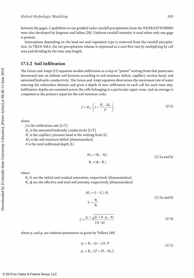
17.3.2 Soil Infiltration

The Green and Ampt [15] equation models infiltration as a step or “piston” wetting front that penetrates downward into an infinite soil horizon according to soil moisture deficit, capillary suction head, and saturated hydraulic conductivity. The Green and Ampt equation determines the maximum rate of water entering the subsurface domain and gives a depth of new infiltration in each cell for each time step. Infiltration depths are summed across the cells belonging to a particular upper zone, and an average is computed as the primary input for the soil moisture code:

f K

H M

Fh

c d= ⋅ + ⋅

1 (17.1)

wheref is the infiltration rate [L/T]Kh is the saturated hydraulic conductivity [L/T]Hc is the capillary pressure head at the wetting front [L]Md is the soil moisture deficit [dimensionless]F is the total infiltrated depth [L]

Md e i

e r

=

=

−

−

( )

( )

θ θ

θ θφ (17.2a and b)

whereθi, θr are the initial and residual saturation, respectively [dimensionless]θe, ϕ are the effective and total soil porosity, respectively [dimensionless]

M S

S

d e e

ei

e

=

=

− ⋅( )1 θ

θθ

(17.3a and b)

f

p p p t

t=

+ + ⋅ ⋅⋅

1 12

28

2 0

∆∆.

(17.4)

where p1 and p2 are solution parameters as given by Velleux [49]

p K t F

p K F H M

h

h c d

1

2

2 0=

=

⋅ − ⋅

⋅ + ⋅( )

∆ . (17.5)


Dow

nloa

ded

by [

Col

orad

o St

ate

Uni

vers

ity L

ibra

ries

], [

Pier

re J

ulie

n] a

t 08:

46 1

3 Ju

ne 2

014


with F, Kh, ∆t, Md, and Hc defined from the previous equations:

t K

H H M

Tl h

w c d= ⋅ + + ⋅

1 (17.6)

wheretl is the transmission loss rate [L/T]Hw is the hydrostatic pressure head of water [L]T is the total depth of transmission losses [L]

17.3.3 Depression Storage

As runoff begins to occur, some of the precipitation excess will be retained in small discontinuous depressions in the land surface. The retained water volume is referred to as depression storage on the land surface and dead storage when it occurs in channels. Dead and depression storage are always subject to infiltration and evaporation. Depression storage acts functionally as a simple abstraction from the volume of water running off of the land surface. For multiple events, dead and depres-sion storage remaining from previous events will contribute to more rapid runoff response in the watershed.

17.3.4 Overland and channel flow routing

TREX-SMA describes conservation of mass and momentum. The diffusive wave approximation of the Saint Venant equation is formulated to estimate the energy grade line or friction slope Sf for both over-land and channel flow. The diffusive wave approximation considers flow generated by differences in head due to depth, as well as bed slope. This allows for flow calculations on horizontal and adverse slopes. Manning roughness derived from land cover and soil type defines flow resistance in energy slope calculations.

The diffusive wave approximation neglects the local and convective acceleration terms of the Saint Venant equations. Richardson and Julien [38] investigated the relative magnitude of all the terms of the Saint Venant equation for overland flow. Their analysis confirms that the neglected terms of the Saint Venant equation are insignificant and that the diffusive approximation is appropriate for most cases of overland flow. In channel flows, Lettenmaier and Wood [28] also showed that the neglected terms of the diffusive wave approximation can become significant when the slope is very small. At California Gulch, with the average slope of 12.5%, the diffusive wave approximation is sufficiently accurate.

Ogden and Julien [32] and Molnár and Julien [30] pointed out that spatial and temporal distributions of rainfall and grid scale may be expected to affect the hydrograph calculations far more than the diffu-sive wave approximation. However, based on their conclusions, the 30 m grid spacing used at California Gulch is adequate to prevent grid-scale effects from influencing the results from this research.

The solution scheme for overland and channel water depth in TREX is the second-order modified Euler scheme (equivalent to the midpoint method of Cheney and Kincaid [8, p. 407]) which uses the cur-rent depth plus an approximate first derivative of the state derived from the prior time step to predict the next time step state. The method uses the unit flow computed from the Manning formulation to predict the depth of water in a model cell in the next time step as detailed in Julien et al. [21] and is known to be unconditionally stable as long as the forward step size satisfies the Courant–Friedrichs–Lewy (CFL) condition [2,9].

In TREX-SMA, surface runoff is calculated with a 2-D formulation of the Saint Venant equation with friction slope in each of x- and y-directions defined using the Manning formulation. Channel flow is computed using 1-D formulations for both continuity and momentum with the diffusive wave


Dow

nloa

ded

by [

Col

orad

o St

ate

Uni

vers

ity L

ibra

ries

], [

Pier

re J

ulie

n] a

t 08:

46 1

3 Ju

ne 2

014


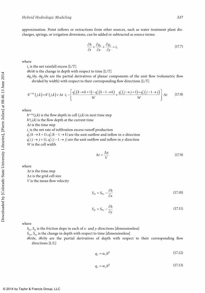
approximation. Point inflows or extractions from other sources, such as water treatment plant dis-charges, springs, or irrigation diversions, can be added or subtracted as source terms:

∂∂

+ ∂∂

+∂∂

=h

t

q

x

q

yix ye (17.7)

whereie is the net rainfall excess [L/T]∂h/∂t is the change in depth with respect to time [L/T]∂qy/∂y, ∂qx/∂x are the partial derivatives of planar components of the unit flow (volumetric flow

divided by width) with respect to their corresponding flow directions [L/T]

h j k h j k t i

q k k q k k

W

q j jt t te

xt

xt

yt

+ ( )= ( )+ −→ +( )− − →( )

+→ +( )∆ ∆, , ⋅

1 1 1 −− − →( )

q j j

Wt

yt 1

⋅∆ (17.8)

whereht+∆t(j,k) is the flow depth in cell (j,k) in next time stepht( j,k) is the flow depth at the current time∆t is the time stepie is the net rate of infiltration excess runoff productionq k kx

t ( );→ +1 q k kxt ( )− →1 are the unit outflow and inflow in x-direction

q j jyt ( );→ +1 q j jy

t ( )− →1 are the unit outflow and inflow in y-directionW is the cell width

∆ ∆

tx

V< (17.9)

where∆t is the time step∆x is the grid cell sizeV is the mean flow velocity

S S

h

xfx x= − ∂

∂0 (17.10)

S S

h

yfy y= − ∂

∂0 (17.11)

whereSfx, Sfy is the friction slope in each of x- and y-directions [dimensionless]S0x, S0y is the change in depth with respect to time [dimensionless]∂h/∂x, ∂h/∂y are the partial derivatives of depth with respect to their corresponding flow

directions [L/L]

q hx x= α β (17.12)

q hy y= α β (17.13)


Dow

nloa

ded

by [

Col

orad

o St

ate

Uni

vers

ity L

ibra

ries

], [

Pier

re J

ulie

n] a

t 08:

46 1

3 Ju

ne 2

014


αx

fxS

n=

1 2/

(17.14)

αy

fyS

n=

1 2/

(17.15)

whereαx, αy is the resistance coefficient in the x- or y-direction [L1/3/T]β is the resistance exponent = 5/3 [dimensionless]n is the Manning roughness coefficient [T/L1/3]

∂∂

+ ∂∂

=A

t

Q

xqc

l (17.16)

whereAc is the cross-sectional area of flow [L2]Q is the total discharge [L3/T]ql is the unit lateral inflow [L2/T]

17.3.5 Soil Moisture accounting in the Upper Zone

In TREX-SMA, the infiltrated water enters the subsurface domain via the upper soil moisture zone. Water is distributed between two portions in the upper zone: the bound water portion (tension water) and the free-flowing portion (free water). Abstractions from the upper zone include evaporation and transpiration, percolation losses to the lower zone, water redistribution, and return flow releases to the surface as interflow.

17.3.5.1 evaporation and Transpiration

Evaporation and transpiration are central to the mass balance in the inter-storm periods. The ET abstraction is removed first from the bound pore water volumes in the model. TREX-SMA currently uses a single constant ET demand for the entire simulation and uniform across the model domain. Any distribution of ET computed from any model could theoretically be used as input since the model aggre-gates the demand from all cells to compute a total ET for each upper zone. ET is first removed from the upper zone tension water based on the ET demand computed from the user-entered potential ET scaled by the available water in the upper zone. If the scaled demand is greater than the amount available in the upper zone tension water storage volume, the additional demand is subtracted from the lower zone ten-sion water storage and the upper zone free water storage. In the present formulation, a simple constant potential ET rate is applied across the model. The free water from the lower zone is not consumed by ET:

ET ET

Fw

Fwactual uz demand

c uz

m uz,

,

,

= ⋅ (17.17)

whereETdemand is the accumulated ET demand for the upper zone for the time step [L]ETactual,uz is the amount of demand removed from the upper zone [L]Fwc,uz is the upper zone free water current storage [L]Fwm,uz is the upper zone free water capacity [L]

In addition to gravity-driven percolation, water in the physical soil column is influenced by capillary forces that drive water movement toward dry soils with a high capillary potential. The tension water


Dow

nloa

ded

by [

Col

orad

o St

ate

Uni

vers

ity L

ibra

ries

], [

Pier

re J

ulie

n] a

t 08:

46 1

3 Ju

ne 2

014


zone represents this capillary soil storage. Following the subtraction of ET losses, a balancing equation transfers excess free water to the tension volume. The transfer occurs when the storage ratio of the ten-sion water is less than the storage ratio of free water. Redistribution exchanges water between the free water and tension water storage until the free and tension water ratios (the current volume divided by maximum storage) are equal.

A similar computation balances the water in the lower zone when the evaporation demand is suf-ficiently high. For the lower zone, the redistribution occurs if the tension water storage ratio is less that the total lower zone storage ratio:

Tw

Tw

Fw

Fwc uz

m uz

c uz

m uz

,

,

,

,

< (17.18)

Tw

Tw

Fw Tw

Fw Twc lz

m lz

c lz c lz

m lz m lz

,

,

, ,

, ,

< ++

(17.19)

The assumption is that if for any reason, the free water storage contains significantly more volume than the tension water than the free water will resupply the tension water. This could happen if the tension water capacity is small relative to the free water capacity and the evaporation is high. This assumption is consistent with the overarching assumption in the Sacramento model that tension water volumes are always satisfied first before any other volumes.

17.3.5.2 Interflow

At each time step, the upper zone free water storage releases water to the surface as interflow. Interflow is computed based on a simple rate equation. An effective depletion coefficient is obtained by multiplying the standard depletion coefficient by the time step.

The upper zone storage depletion coefficient defines the flow released per volume of stored water in the zone, normalized by the area of the model contributing to the given zone. The internal units of the soil moisture accounting procedure are 1-D length (e.g., millimeters) so the outgoing flow is scaled by the upper zone area. As used in the Sacramento model implemented in NWSRFS, the standard upper zone depletion coefficient is calibrated in units of millimeters released per millime-ters stored per day. More specifically, the TREX-SMA model uses a conversion factor to account for different time steps:

V k Fwf uz eff c uzint = ⋅, , (17.20)

whereVintf is the baseflow unit volume for the time step [L]Fwc,uz is the current unit volume of upper zone free water [L]kuz,eff is the effective upper zone free water storage depletion coefficient [dimensionless]

k k tuz eff uz, = ⋅∆ (17.21)

wherekuz is the standard upper zone free water storage depletion coefficient [L/(L · T)]∆t is the current model time step [T]

V k t Fwf uz c uzint = ⋅ ⋅ ⋅ ⋅∆ , Area Conversion factors (17.22)


Dow

nloa

ded

by [

Col

orad

o St

ate

Uni

vers

ity L

ibra

ries

], [

Pier

re J

ulie

n] a

t 08:

46 1

3 Ju

ne 2

014


or written to emphasize the units as

V k t Fwf uz eff c uzint = ⋅ ⋅ ⋅ ⋅

=

, ,∆ Area Conversion factors

mmm

mm3

⋅⋅days mm m

meter

mm

day

s

⋅[ ] ⋅[ ] ⋅ ⋅ ⋅

2

1 000

1

86 400, , (17.23)

Similar scaling is required to obtain an effective storage depletion coefficient for the lower zone free water storage depletion coefficients, taking into consideration the time step and also scaling from the NWSRFS parameter range that is used in TREX-SMA.

17.3.6 Soil Moisture accounting in the Lower Zone

Water drains into the lower zone via percolation. Losses from the lower zone include ET and baseflow.

17.3.6.1 Percolation

Water is transferred from the upper zones to the lower zones via the percolation computation. The percolation demand is computed as a demand in millimeters per day. A conversion is applied to determine the effec-tive demand for the relatively small time steps occurring in the TREX-SMA model. The lower zone percola-tion demand (demand for water from the upper zone to fill lower zone free water storages) is computed from a base percolation rate parameter and a two-parameter percolation curve that multiplies the percolation rate based on the current free water state. The actual percolation is reduced from the percolation demand based on the availability of upper zone free water. The total volume removed is limited by the amount in the upper zone free water current storage volume, to prevent mass balance errors. More specifically,

Perc Perc zperc

a

bdemand base

r

= ⋅ + ⋅

1

exp

(17.24)

wherePercdemand is the percolation demand [L/T]Percbase is the base percolation rate [L/T]zperc is the percolation multiplierrexp is the wet vs. dry percolation differentiation exponentfactors a and b define the aggregate lower zone deficiency ratio:

a

b

Tw Fw Tw Fw

Tw Fwm lz m lz c lz c lz

m lz m lz

= + − ++

, , , ,

, ,

Σ ΣΣ

(17.25)

Perc Perc

Fw

FwFwactual demand eff

c uz

m uzc uz= ⋅ ≤,

,

,, (17.26)

17.3.6.2 Baseflow

In TREX-SMA, the baseflow is returned to surface runoff as a point source as calculated from

V k Fwbasf lz eff c lz= ⋅, , (17.27)

whereVbasf is the baseflow volume [L]klz,eff = klz[L/(L · T)] · ∆t[T] is the effective lower zone free water storage depletion coefficient

[dimensionless]


Dow

nloa

ded

by [

Col

orad

o St

ate

Uni

vers

ity L

ibra

ries

], [

Pier

re J

ulie

n] a

t 08:

46 1

3 Ju

ne 2

014


In order to allow multi-event simulation with TREX-SMA, the saturation condition of the soil moisture is used to re-initialize the parameters of the Green and Ampt infiltration equation:

SMA summary state = ∑∑

Tw Fw Tw

Tw Fw Tw

c uz c uz c lz

m uz m uz m l

, , ,

, , ,

, ,

, , zz

(17.28)

Infiltration parameters remain fixed for the duration of each storm and are allowed to recover soil moisture deficit between storms due to ET and drainage. In SMA, a storm ends at cessation of rainfall, when the precipitated water falls below a user-entered threshold value. The model does not change the infiltration parameters immediately upon cessation of rainfall, but continues to allow infiltration to occur using the Green and Ampt parameters set at the beginning of each storm.

17.4 Hybrid Modeling application at california Gulch

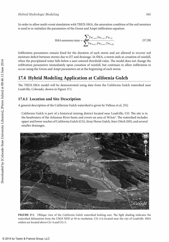
The TREX-SMA model will be demonstrated using data from the California Gulch watershed near Leadville, Colorado, shown in Figure 17.1.

17.4.1 Location and Site Description

A general description of the California Gulch watershed is given by Velleux et al. [51]:

California Gulch is part of a historical mining district located near Leadville, CO. The site is in the headwaters of the Arkansas River basin and covers an area of 30 km2. The watershed includes upper and lower reaches of California Gulch (CG), Stray Horse Gulch, Starr Ditch (SD), and several smaller drainages.

FIGuRE 17.1 Oblique view of the California Gulch watershed looking east. The light shading indicates the watershed delineation from the USGS NED at 30 m resolution. CG-4 is located near the city of Leadville. SMA outlets are located above CG-4 and CG-5.


Dow

nloa

ded

by [

Col

orad

o St

ate

Uni

vers

ity L

ibra

ries

], [

Pier

re J

ulie

n] a

t 08:

46 1

3 Ju

ne 2

014


Due to the history of surface mine waste accumulation, the area of California Gulch was added to the US EPA National Priority List in 1983 [16,48]. The national priority list sites are designated as part of the Comprehensive Environmental Response, Compensation, and Liability Act (CERCLA) commonly known as Superfund [48].

17.4.2 elevation and Topography

Elevations in the watershed range from 2,900 m (9,600 ft) at the Arkansas River to 3,650 m (12,000 ft) on top of Ball Mountain at the eastern boundary of the watershed. The average slope is 12.6% [51]. The city of Leadville, roughly in the center of the watershed, contains a small watershed divide between California Gulch and Malta Gulch with the majority of runoff from the city draining into California Gulch. The deep channel of California Gulch dominates the general topography of the valley as it runs from the bedrock formations of the upper watershed down through the alluvium and glacial deposits in the lower watershed.

The USGS 1/3rd arc second digital elevation model (DEM) from the National Elevation Dataset (NED) provides the basis for all topographic computations in the model. The site was simulated on a 30 m × 30 m grid based on the nominal dimensions of the NED, and the watershed area was delineated with 34,002 cells for the overland plane. All other distributed inputs were converted to the same spac-ing for purposes of calculation. The model setup from Velleux et al. [51] was replicated for use with the TREX-SMA simulations.

17.4.3 Land Use

In the TREX-SMA model, land use classification is used to determine overland flow roughness and interception depth. The NLCD 2001 land use dataset from NASA and USGS distinguishes 13 differ-ent land use classes in the California Gulch watershed. Evergreen forest dominates the majority of the watershed except for the urban area of Leadville, and mining or otherwise industrially impacted lands that are classified as either “commercial” or “bare rock.”

17.4.4 Soil Type

Within the watershed, the USDA identifies 14 different soil associations. These were used along with a separate class for soils within the city of Leadville urbanized (subdivided by land use) to create a total of 17 soil classes for the model.

The characteristics (Kh, Hc, K, porosity, grain size distribution, etc.) of each soil class were defined based on values reported in the NRCS SSURGO database as well as texture.

The method of Rawls et al. [34,35] was used to generate initial values for the Green and Ampt param-eters (saturated hydraulic conductivity and capillary suction head) for use in the model. Kh values were calibrated by Velleux et al. [51] to achieve agreement between measured and simulated runoff.

17.4.5 Temperature

Hourly air temperature data were obtained for the modeling period from the Western Regional Climate Center (WRCC) for the weather station at the Leadville airport 5 km (3.2 mile) south of Leadville. The Leadville airport gage is at 9,938 ft above mean sea level. A normal adiabatic lapse rate of 3.6°F per 1,000 ft would predict temperatures approximately 8°F cooler at the top of Ball Mountain (elevation 12,300 ft) and 1°F warmer at the watershed outlet (elevation 9,530 ft) into the Arkansas River. The climate record shows that daily extremes stayed well above freezing for nearly all the simulated period eliminating concern about frozen ground effects.


Dow

nloa

ded

by [

Col

orad

o St

ate

Uni

vers

ity L

ibra

ries

], [

Pier

re J

ulie

n] a

t 08:

46 1

3 Ju

ne 2

014


17.4.6 evapotranspiration

The inter-event recovery of infiltration capacity in the soil moisture zones of TREX-SMA is driven by the release of water to the channel and by ET [43]. Pan evaporation has been measured at the Sugarloaf Reservoir weather station operated by the Bureau of Reclamation since 1948. The pan is located south-east of the dam at 39°15′ north and 106°22′ west at an elevation of 2968 m (9738 ft), approximately 7 km (4.4 mile) west of the City of Leadville and 125 m (410 ft) lower in elevation. During summer months, when snow cover is largely absent, the values from the Sugarloaf Pan should be indicative of conditions in California Gulch [17].

Monthly evaporation values from the WRCC data show that for the months of July and August 2006, evaporation was less than the corresponding cumulative monthly averages for 1948 through 2005 [31]. The reduced evaporation is related to the occurrence of more precipitation that usual, one reason why this summer period was chosen for simulation.

Daily records from the pan show fluctuations between nearly 0 and 0.32 in. per day for July and August 2006. For purposes of simulation, the 2006 monthly averages from the WRCC were used to compute an average potential ET rate of 5.6 in. per month. This value was applied as a constant demand during all simulations.

17.4.7 Precipitation

As part of the CERCLA/Superfund efforts in California Gulch, a program to monitor the impact of mine waste transport on Arkansas River ecology, a network of automated pluviographic and fluvial gaging stations was established by the EPA. Automated sampling stations were installed each summer from 2003 through 2008 approximately from June through September. The automated sampling program 2009 and 2010 only included the peak runoff season. Gage locations and descriptions are given in Table 17.2. Precipitation and channel flow are recorded at 10 min intervals for stations labeled as CG-1, SHG-09, CG-4, and CG-6, and measurements are also made at locations CG-5, SD-3A, OG-1, AR-1, and AR-3A.

The summer of 2006 included at least eight significant convective storms with measurable precipita-tion recorded at all four automated pluvial gaging stations. A series of nine storms from summer 2006 were used as input to test the multi-event simulation capabilities of the TREX-SMA model. The first and most intense storm in the series occurred on July 19 (the same used for the baseflow modeling simula-tion). The subsequent storms occurred on a roughly weekly basis following the first storm on July 25/26, July 30/31, August 5/6, and August 10/11. All of these storms occurred when snowmelt influences on streamflow in California Gulch had largely subsided for the summer.

TABLE 17.2 Automated Gage Locations and Available Data

Gage Description Available Data

SHG-09 300 ft below Emmett retention pond 1, 2, 3, 4, 5, 6SD-3A Flume in Starr Ditch downstream of Monroe St. and upstream of drop structure 1, 2, 3, 4, 5CG-1 California Gulch immediately upstream of the Yak Tunnel portal 1, 2, 3, 4, 5, 6OG-1 Oregon Gulch immediately upstream of confluence with California Gulch 1, 2, 3, 4, 5CG-4 California Gulch downstream of confluence with Oregon Gulch 1, 2, 3, 4, 5, 6CG-5 California Gulch upstream of the Leadville Wastewater Treatment Plant 1, 2, 3, 4, 5CG-6 California Gulch immediately upstream of confluence with Arkansas River 1, 2, 3, 4, 5, 6AR-1 Arkansas River upstream of confluence with California Gulch, approximately 0.25 miles

downstream of the confluence with Tennessee Creek1, 2, 3, 4, 5

AR-3A Arkansas River approximately 0.5 mile downstream of confluence with California Gulch 1, 2, 3, 4, 5

1, Stage; 2, discharge; 3, temperature; 4, conductivity; 5, pH; 6, precipitation.


Dow

nloa

ded

by [

Col

orad

o St

ate

Uni

vers

ity L

ibra

ries

], [

Pier

re J

ulie

n] a

t 08:

46 1

3 Ju

ne 2

014


During the July 19th storm, the most intense precipitation was measured in SHG at the SHG-09A gage, registering 0.4 in. in 10 min, equivalent to an intensity of 2.4 in./h. For comparison, a 100-year, 2 h storm for the watershed would reach 0.87 in./h, distributed over the watershed [44].

The observations at the four different precipitation gages show that the storms vary in geographic dis-tribution. Throughout the summer, storms were recorded in which not all gages received precipitation. Many of these were biased toward the upper watershed (near CG-1 and SHG-09A). For instance, the August 6th storm was an upper watershed storm that generated significant flow at CG-1 but at no other gage. A simple weighting scheme placing the centroid of the total precipitation along the East–West axis of the watershed classified each storm as primarily upper or lower watershed.

17.4.8 Stream flow

Data from 2003 through 2007 were evaluated to find a suitable modeling period. The precipitation and streamflow hydrographs from the automatic gaging stations during a nonsnowmelt period at the end of the summer of 2006 were selected for testing TREX-SMA. Several large precipitation peaks and cor-respondingly significant runoff signatures allow examining simulation quality during both high and low flows.

17.4.9 Hybrid Model Parameters

All surface model parameters for the multi-event simulation were drawn from the model calibration and validation by Velleux [49]. These calibrated parameters have been used for several event-based sim-ulations of contaminant transport as seen in two papers by Velleux et al. [50–52] and further discussed by Caruso et al. [7]. Related work in the same basin has also been published by Rojas-Sánchez et al. [41] and for the simulation of extreme events including the PMP–PMF by England et al. [14].

For the multi-event simulation reported in this chapter, parameters for the SMA zones were drawn from the a priori dataset described by Koren et al. [26]. The parameter values are determined a priori using soils and land use data and are used by scientists at the NWS Arkansas Basin River Forecast Center (ABRFC) for regional hydrologic forecasting using the NWS distributed hydrologic model (DHM) [25]. For this research, the parameters from the three 4 km × 4 km grid cells aligned east and west nearest to Leadville (those most nearly corresponding to the California Gulch watershed area) were averaged to provide values for use in modeling, which are shown in Table 17.3.

17.5 TreX-SMa results and Discussion

17.5.1 Multi-event Simulation Hydrographs

We applied the TREX-SMA model to a real case at California Gulch in which 50 days of precipitation inputs were used to drive a model simulation. The multi-event simulation was carried out twice: once with the SMA submodel active, resetting the infiltration parameters at appropriate times, and once again with no infiltration resetting. The simulations and their respective results are distinguished in this discussion as “SMA” for the hybrid TREX-SMA simulations and “no-SMA” for TREX simulations without SMA.

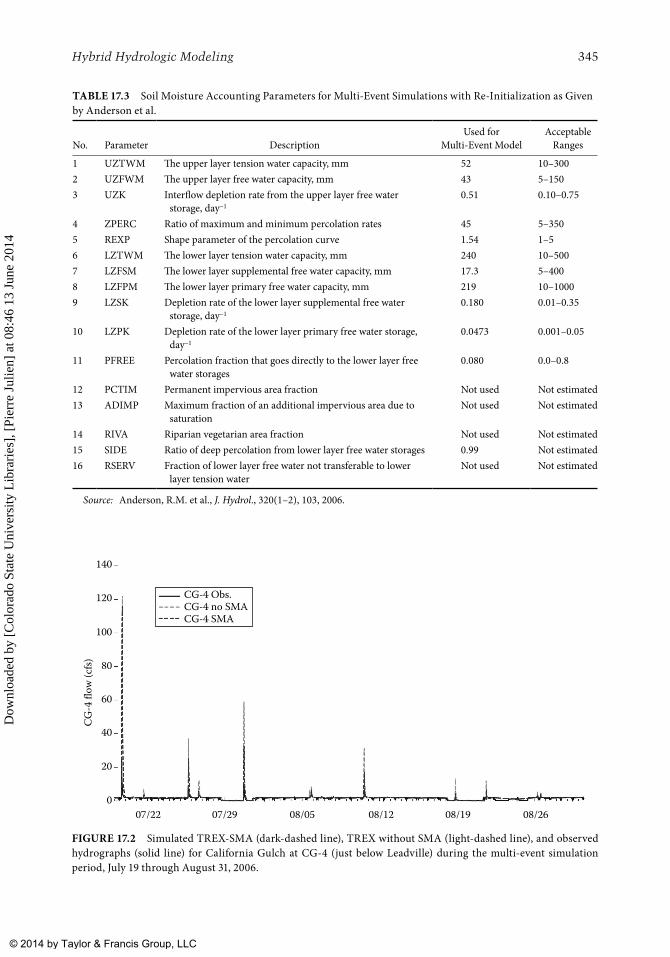
The basin hydrologic response is captured most succinctly in the hydrographs showing the flow as a function of time through the simulated period. As expected, the TREX-SMA simulation reduces the simulated hydrograph peaks, especially for storms later in the series as the SMA zones dry out toward the end of summer. Figure 17.2 shows the aggregate basin response at CG-4 near Leadville for simula-tions with and without the SMA submodel. Observed flows are also shown on the plot, for comparison to the simulated flow. The graphical evidence of the reduced peaks shown in these figures is the most


Dow

nloa

ded

by [

Col

orad

o St

ate

Uni

vers

ity L

ibra

ries

], [

Pier

re J

ulie

n] a

t 08:

46 1

3 Ju

ne 2

014


TABLE 17.3 Soil Moisture Accounting Parameters for Multi-Event Simulations with Re-Initialization as Given by Anderson et al.

No. Parameter DescriptionUsed for

Multi-Event ModelAcceptable

Ranges

1 UZTWM The upper layer tension water capacity, mm 52 10–3002 UZFWM The upper layer free water capacity, mm 43 5–1503 UZK Interflow depletion rate from the upper layer free water

storage, day−10.51 0.10–0.75

4 ZPERC Ratio of maximum and minimum percolation rates 45 5–3505 REXP Shape parameter of the percolation curve 1.54 1–56 LZTWM The lower layer tension water capacity, mm 240 10–5007 LZFSM The lower layer supplemental free water capacity, mm 17.3 5–4008 LZFPM The lower layer primary free water capacity, mm 219 10–10009 LZSK Depletion rate of the lower layer supplemental free water

storage, day−10.180 0.01–0.35

10 LZPK Depletion rate of the lower layer primary free water storage, day−1

0.0473 0.001–0.05

11 PFREE Percolation fraction that goes directly to the lower layer free water storages

0.080 0.0–0.8

12 PCTIM Permanent impervious area fraction Not used Not estimated13 ADIMP Maximum fraction of an additional impervious area due to

saturationNot used Not estimated

14 RIVA Riparian vegetarian area fraction Not used Not estimated15 SIDE Ratio of deep percolation from lower layer free water storages 0.99 Not estimated16 RSERV Fraction of lower layer free water not transferable to lower

layer tension waterNot used Not estimated

Source: Anderson, R.M. et al., J. Hydrol., 320(1–2), 103, 2006.

140

CG-4

flow

(cfs)

120

100

80

60

40

20

0

CG-4 Obs.CG-4 no SMACG-4 SMA

07/22 07/29 08/05 08/12 08/19 08/26

FIGuRE 17.2 Simulated TREX-SMA (dark-dashed line), TREX without SMA (light-dashed line), and observed hydrographs (solid line) for California Gulch at CG-4 (just below Leadville) during the multi-event simulation period, July 19 through August 31, 2006.


Dow

nloa

ded

by [

Col

orad

o St

ate

Uni

vers

ity L

ibra

ries

], [

Pier

re J

ulie

n] a

t 08:

46 1

3 Ju

ne 2

014


convincing measure of the improvement brought with the SMA re-initialization procedure. For most storms, the no-SMA case overpredicts the basin response, while the reduced SMA peak corresponds more closely to the observed flow.

Generally speaking, the hydrographs show that the TREX-SMA model has reduced the overpredic-tion of peaks. Only the SHG-09A hydrograph seems unmodified—the soil types in that portion of the watershed have such low infiltration rates that the differences in soil moisture do little to increase or decrease the infiltration. The inter-event periods show apparently very good fit to observed data for both SMA and no-SMA cases.

17.5.2 Overall Statistical Performance

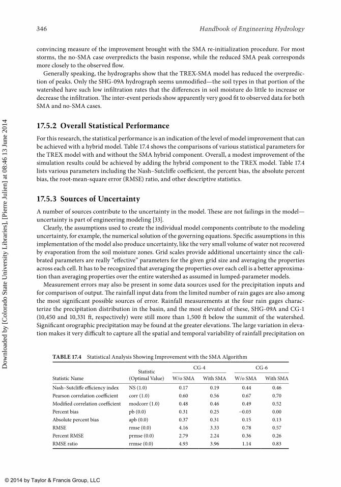
For this research, the statistical performance is an indication of the level of model improvement that can be achieved with a hybrid model. Table 17.4 shows the comparisons of various statistical parameters for the TREX model with and without the SMA hybrid component. Overall, a modest improvement of the simulation results could be achieved by adding the hybrid component to the TREX model. Table 17.4 lists various parameters including the Nash–Sutcliffe coefficient, the percent bias, the absolute percent bias, the root-mean-square error (RMSE) ratio, and other descriptive statistics.

17.5.3 Sources of Uncertainty

A number of sources contribute to the uncertainty in the model. These are not failings in the model—uncertainty is part of engineering modeling [33].

Clearly, the assumptions used to create the individual model components contribute to the modeling uncertainty, for example, the numerical solution of the governing equations. Specific assumptions in this implementation of the model also produce uncertainty, like the very small volume of water not recovered by evaporation from the soil moisture zones. Grid scales provide additional uncertainty since the cali-brated parameters are really “effective” parameters for the given grid size and averaging the properties across each cell. It has to be recognized that averaging the properties over each cell is a better approxima-tion than averaging properties over the entire watershed as assumed in lumped-parameter models.

Measurement errors may also be present in some data sources used for the precipitation inputs and for comparison of output. The rainfall input data from the limited number of rain gages are also among the most significant possible sources of error. Rainfall measurements at the four rain gages charac-terize the precipitation distribution in the basin, and the most elevated of these, SHG-09A and CG-1 (10,450 and 10,331 ft, respectively) were still more than 1,500 ft below the summit of the watershed. Significant orographic precipitation may be found at the greater elevations. The large variation in eleva-tion makes it very difficult to capture all the spatial and temporal variability of rainfall precipitation on

TABLE 17.4 Statistical Analysis Showing Improvement with the SMA Algorithm

Statistic NameStatistic

(Optimal Value)

CG-4 CG-6

W/o SMA With SMA W/o SMA With SMA

Nash–Sutcliffe efficiency index NS (1.0) 0.17 0.19 0.44 0.46Pearson correlation coefficient corr (1.0) 0.60 0.56 0.67 0.70Modified correlation coefficient modcorr (1.0) 0.48 0.46 0.49 0.52Percent bias pb (0.0) 0.31 0.25 −0.03 0.00Absolute percent bias apb (0.0) 0.37 0.31 0.15 0.13RMSE rmse (0.0) 4.16 3.33 0.78 0.57Percent RMSE prmse (0.0) 2.79 2.24 0.36 0.26RMSE ratio rrmse (0.0) 4.93 3.96 1.14 0.83


Dow

nloa

ded

by [

Col

orad

o St

ate

Uni

vers

ity L

ibra

ries

], [

Pier

re J

ulie

n] a

t 08:

46 1

3 Ju

ne 2

014


this watershed. This is especially critical because about 95% of the water infiltrates in these simulations, so infiltration location will play a large role in the timing of flood peak arrival.

17.5.4 advances in Model Visualization

A hydrologic model consists of a hydrologic core and a separate technological shell that is “the pro-gramming, user interface, pre- and postprocessing facilities, etc.” [37]. GIS in modeling serves to assist where “the hydrologist needs to cooperate intensively with experts in the field of ecology, agriculture, urban planning, and economics” [13]. This is because “the pure numerical results of a simulation are no longer the final products delivered by the hydrologist. The results have to be translated systematically into hydrological effects and subsequently into socially relevant quantities … [so that] the hydrologist can no longer depend on tabular representations of his data … [and] graphical tools [are] a necessity” [10]. Johnson et al. [19] state that the spatial capabilities of the model combined with GIS data for input parameters are the raison d’être for CASC2D-SED: “The strength of the model CASC2D-SED lies in its tremendous potential and visual output….”

Viewing the model output in the context of the geography and other imagery is useful for at least two reasons. First, the visual comparison of topography and other geographic and spatial features allows for a rapid evaluation of the success of the simulation. Model output is visually compared to expectation similar to the visual comparison on observed and simulated hydrographs on a plot. Second, the primary consumers of the information from a hydrologic model will have questions with specific respect to loca-tion of effects such as overbank flow, points of maximum velocity, and scour problem areas. All of these effects may be evaluated with the TREX-SMA model.

The Google Earth™ viewer allows browsing of the series of overlays in both time and space. Any area may be highlighted for close viewing and the entire series may be animated or a particular time chosen using a time selector in the Google Earth™ interface. Other data such as gage locations may be inserted for additional context.

17.5.5 results Displayed with KML

In order to further evaluate the simulation results, a 3-D interactive results display was implemented using Google Earth™ and the Keyhole Markup Language (KML). Google Earth™ is a web-based “vir-tual globe” that shows a 3-D view of the earth’s surface in varying resolutions based on various sources of aerial imagery and digital terrain models. The KML is an xml-based scripting language designed to allow display of text and graphics on a virtual globe such as Google Earth™ [36,53].

To use Google Earth™ to display TREX-SMA results, grid cell values of the land surface and chan-nel water depth were exported from the model simulation at given time intervals as raster images, and these images were ingested into a GRASS GIS database [29]. The maps were colorized according to the data values for each cell and then exported as a flat graphic that is referenced as a ground overlay in a simple KML file. The KML file specifies the spatial and temporal extent of the overlay (e.g., an overlay may represent the average model states from 12:00 am to 12:10 am of July 30, 2006, and have a north, south, east, and west maximum extent). The KML time points were specified along with an offset from GMT and positions using latitude and longitude. The appropriate KML tags were inserted to specify the transparency of each overlay to allow partial viewing of the standard Google Earth™ aerial image underneath the overlay showing the modeled value. The ground overlays were produced to show depth of flow (on the land surface and in channels) but could show any other distributed variable from the TREX-SMA output. The Google Earth™ interface also allows for the series of individual frames to be animated showing evolution of model processes over time.

A demonstration of these graphical methods was performed using an application of TREX by Velleux [49] at California Gulch near Leadville, Colorado. The 100-year storm was simulated as 1.73 in. of uniformly distributed rain falling in 2 h over the entire watershed. The 100-year analysis was used to


Dow

nloa

ded

by [

Col

orad

o St

ate

Uni

vers

ity L

ibra

ries

], [

Pier

re J

ulie

n] a

t 08:

46 1

3 Ju

ne 2

014


demonstrate the effect of applying the improved graphical techniques. To produce the animation, the same process described previously was used to create flat frames showing the depth of water on the land surface at various times through the simulation. The color maps were produced according to the data values for each cell and then draped on a DEM, also contained in the GIS.

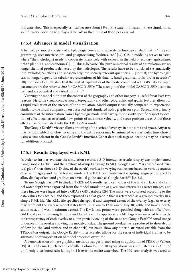
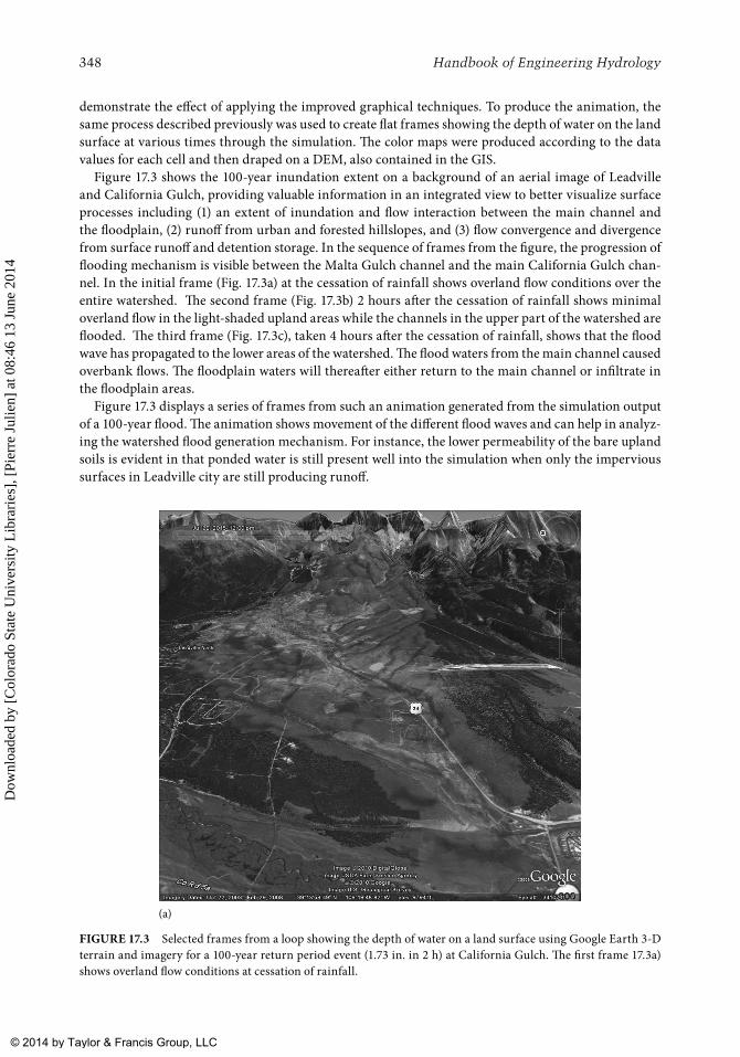
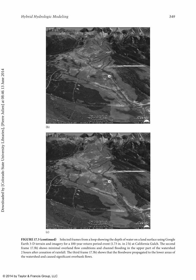
Figure 17.3 shows the 100-year inundation extent on a background of an aerial image of Leadville and California Gulch, providing valuable information in an integrated view to better visualize surface processes including (1) an extent of inundation and flow interaction between the main channel and the floodplain, (2) runoff from urban and forested hillslopes, and (3) flow convergence and divergence from surface runoff and detention storage. In the sequence of frames from the figure, the progression of flooding mechanism is visible between the Malta Gulch channel and the main California Gulch chan-nel. In the initial frame (Fig. 17.3a) at the cessation of rainfall shows overland flow conditions over the entire watershed. The second frame (Fig. 17.3b) 2 hours after the cessation of rainfall shows minimal overland flow in the light-shaded upland areas while the channels in the upper part of the watershed are flooded. The third frame (Fig. 17.3c), taken 4 hours after the cessation of rainfall, shows that the flood wave has propagated to the lower areas of the watershed. The flood waters from the main channel caused overbank flows. The floodplain waters will thereafter either return to the main channel or infiltrate in the floodplain areas.

Figure 17.3 displays a series of frames from such an animation generated from the simulation output of a 100-year flood. The animation shows movement of the different flood waves and can help in analyz-ing the watershed flood generation mechanism. For instance, the lower permeability of the bare upland soils is evident in that ponded water is still present well into the simulation when only the impervious surfaces in Leadville city are still producing runoff.

(a)

FIGuRE 17.3 Selected frames from a loop showing the depth of water on a land surface using Google Earth 3-D terrain and imagery for a 100-year return period event (1.73 in. in 2 h) at California Gulch. The first frame 17.3a) shows overland flow conditions at cessation of rainfall.


Dow

nloa

ded

by [

Col

orad

o St

ate

Uni

vers

ity L

ibra

ries

], [

Pier

re J

ulie

n] a

t 08:

46 1

3 Ju

ne 2

014


(b)

(c)

FIGuRE 17.3 (continued) Selected frames from a loop showing the depth of water on a land surface using Google Earth 3-D terrain and imagery for a 100-year return period event (1.73 in. in 2 h) at California Gulch. The second frame 17.3b) shows minimal overland flow conditions and channel flooding in the upper part of the watershed 2 hours after cessation of rainfall. The third frame 17.3b) shows that the floodwave propagated to the lower areas of the watershed and caused significant overbank flows.


Dow

nloa

ded

by [

Col

orad

o St

ate

Uni

vers

ity L

ibra

ries

], [

Pier

re J

ulie

n] a

t 08:

46 1

3 Ju

ne 2

014


17.6 Summary and conclusions

A new hybrid approach to hydrologic modeling combines distributed surface runoff modeling with a lumped-parameter rendering of infiltration and subsurface flow. The hybrid model TREX-SMA com-bines the SAC-SMA model with the TREX surface hydrology model. The capabilities of hybrid model-ing are demonstrated with an application to the 30 km2 California Gulch watershed, near Leadville, Colorado. The results of a 50-day simulation are presented for comparisons with and without the hybrid model component SMA. Surface runoff parameters were obtained from a prior calibration of TREX, and the SMA soil moisture parameters were determined from a priori estimates used by the ABRFC of the NWS. The hybrid simulation results with TREX-SMA improved relative to results from the unmodi-fied TREX model. Model results such as surface and channel water depth are processed with GRASS GIS and KML scripts to create 2.5-D, browsable animations overlaid on a Google Earth™ terrain.

references

1. Abbott, M.B. and Refsgaard, J.C. 1996. Distributed Hydrological Modelling. Springer, Heidelberg, Germany.

2. Alexiades, V., Amiez, G., and Gremaud, P.A. 1996. Super-time-stepping acceleration of explicit schemes for parabolic problems. Communications in Numerical Methods in Engineering, 12(1), 31–42.

3. Anderson, R.M., Koren, V.I., and Reed, S.M. 2006. Using SSURGO data to improve Sacramento Model a priori parameter estimates. Journal of Hydrology, 320(1–2), 103–116.

4. Aral, M.M. and Gunduz, O. 2003. Scale effects in large scale watershed modeling. In Advances in Hydrology, V.P. Singh and R.N. Yadava, eds., Allied Publishers, New Delhi, India, pp. 37–51.

5. Aral, M.M. and Gunduz, O. 2006. Large-scale hybrid watershed modeling. In Watershed Models, V.P. Singh and D.K. Frevert, eds., CRC/Taylor & Francis Group, Boca Raton, FL, pp. 75–95.

6. Burnash, R. and Ferral, L. 2002. Conceptualization of the Sacramento soil moisture accounting model. NWSRFS User Manual Documentation, National Weather Service, NOAA, Silver Spring, MD.

7. Caruso, B.S., Cox, T.J., Runkel, R.L., Velleux, M.L., Bencala, K.E., Nordstrom, D.K., Julien, P.Y., Butler, B.A., Alpers, C.N., Marion, A., and Smith, K.S. 2008. Metals fate and transport modelling in streams and watersheds: State of the science and USEPA workshop review. Hydrological Processes, 22(19), 4011–4021.

8. Cheney, W. and Kincaid, D. 1999. Numerical Mathematics and Computing. Brooks/Cole Pub Co., Pacific Grove, CA.

9. Courant, R., Friedrichs, K., and Lewy, H. 1928. Über die partiellen Differenzengleichungen der mathematischen Physik. Mathematische Annalen, 100(1), 32–74.

10. Deckers, F. and Te Stroet, C.B.M. 1996. Use of GIS and database with distributed modelling. In Distributed Hydrological Modelling, M.B. Abbott and J.C. Refsgaard, eds., Springer, Heidelberg, Germany pp. 215–216.

11. Dunne, T. and Black, R.D. 1970. An experimental investigation of runoff production in permeable soils. Water Resources Research, 6(2), 478–490.

12. Dunne, T. and Black, R.D. 1970. Partial area contributions to storm runoff in a small New England watershed. Water Resources Research, 6(5), 1296–1311.

13. Engelen, G.B. and Kloosterman, F.H. 1996. Hydrological Systems Analysis: Methods and Applications. Water Science and Technology Library, Kluwer, Dordrecht, the Netherlands.

14. England, J.F., Velleux, M.L., and Julien, P.Y. 2007. Two-dimensional simulations of extreme floods on a large watershed. Journal of Hydrology, 347(1–2), 229–241.

15. Green, W.H. and Ampt, G.A. 1911. Studies on soil physics. Part I—The flow of air and water through soils. Journal of Agricultural Science, 4, 1–24.


Dow

nloa

ded

by [

Col

orad

o St

ate

Uni

vers

ity L

ibra

ries

], [

Pier

re J

ulie

n] a

t 08:

46 1

3 Ju

ne 2

014


16. HDR. 2002. Final focused feasibility study for operable unit 6, California Gulch NPL Site, Leadville Colorado, HDR Engineering, Omaha, NE.

17. Henning, I. and Henning, D. 1981. Potential evapotranspiration in mountain geoecosystems of dif-ferent altitudes and latitudes. Mountain Research and Development, 1(3/4), 267–274.

18. Johnson, B.E. 1997. Development of a storm event based two-dimensional upland erosion model. PhD dissertation, Department of Civil Engineering, Colorado State University, Fort Collins, CA.

19. Johnson, B.E., Julien, P.Y., Molnár, D.K., and Watson, C.C. 2000. The two-dimensional upland ero-sion model CASC2D-SED. Journal of the American Water Resources Association, 36(1), 31–42.

20. Jorgeson, J. and Julien, P.Y. 2005. Peak flow forecasting with CASC2D and radar data. Special Issue, Water International, International Water Resources Association, IWRA, 30(1), 40–49.

21. Julien, P.Y., Saghafian, B., and Ogden, F.L. 1995. Raster-based hydrologic modeling of spatially-varied surface runoff. Water Resources Bulletin, 31(3), 523–536.

22. Kampf, S.K. and Burges, S.J. 2007. A framework for classifying and comparing distributed hillslope and catchment hydrologic models. Water Resources Research, 43, 24.

23. Kavvas, M.L., Chen, Z.Q., Dogrul, C., Yoon, J.Y., Ohara, N., Liang, L., Aksoy, H., Anderson, M.L., Yoshitani, J., Fukami, K., and Matsuura, T. 2004. Watershed Environmental Hydrology (WEHY) model based on upscaled conservation equations: Hydrologic module. Journal of Hydrologic Engineering, 9(6), 450–464.

24. Kirchner, J.W. 2003. A double paradox in catchment hydrology and geochemistry. Hydrological Processes, 17(4), 871–874.

25. Koren, V.I., Reed, S.M., Smith, M.B., Zhang, Z., and Seo, D.-J. 2004. Hydrology laboratory research modeling system (HL-RMS) of the US national weather service. Journal of Hydrology, 291(3–4), 297–318.

26. Koren, V.I., Smith, M.B., and Duan, Q. 2003. Use of a priori parameter estimates in the deriva-tion of spatially consistent parameter sets of rainfall–runoff models. In Calibration of Watershed Models (Water Science and Application), Q. Duan, H.V. Gupta, S. Sorooshian, A.N. Rousseau, and R. Turcotte, eds., American Geophysical Union, Washington, DC, pp. 239–254.

27. Koren, V.I., Smith, M.B., Wang, D., and Zhang, Z. 2000. Use of soil property data in the deriva-tion of conceptual rainfall–runoff model parameters. 15th Conference on Hydrology, American Meteorological Society, Long Beach, CA, 403pp.

28. Lettenmaier, D.P. and Wood, E.F. 1993. Hydrologic forecasting. In Handbook of Hydrology, D.R. Maidment, ed., McGraw-Hill, New York, pp. 26.1–26.30.

29. Neteler, M. and Mitrasova, H. 2008. Open Source GIS: A Grass GIS Approach. Springer Verlag, New York.

30. Molnár, D.K. and Julien, P.Y. 2000. Grid-size effects on surface runoff modeling. Journal of Hydrologic Engineering, 5(1), 8–16.

31. National Climatic Data Center. 2010. NCDC: Weather station. http://www4.ncdc.noaa.gov/cgi-win/wwcgi.dll?wwDI%7EStnSrch%7EStnID%7E20003674 (June 4, 2010).

32. Ogden, F.L. and Julien, P.Y. 1993. Runoff sensitivity to temporal and spatial rainfall variability at runoff plane and small basin scales. Water Resources Research, 29(8), 2589–2597.

33. Pappenberger, F., Beven, K.J., Hunter, N.M., Bates, P.D., Gouweleeuw, B.T., Thielen, J., and De Roo, A.P.J. 2005. Cascading model uncertainty from medium range weather forecasts (10 days) through a rainfall–runoff model to flood inundation predictions within the European Flood Forecasting System (EFFS). Hydrology and Earth System Sciences, 9(4), 381–393.

34. Rawls, W.J., Brakensiek, D.L., and Saxton, K.E. 1982. Estimation of soil water properties. Transactions of the ASAE, 25(5), 1328–1320.

35. Rawls, W.J., Brakensiek, D.L., and Miller, N. 1983. Green-Ampt infiltration parameters from soils data. Journal of Hydraulic Engineering, 109(1), 62–70.

36. Reed, S.M. and Halgren, J.S. 2011. Validation of a new GIS tool to rapidly develop simplified dam break models. Dam Safety 2011, Association of State Dam Safety Officials, Washington, DC.


Dow

nloa

ded

by [

Col

orad

o St

ate

Uni

vers

ity L

ibra

ries

], [

Pier

re J

ulie

n] a

t 08:

46 1

3 Ju

ne 2

014

http://www4.ncdc.noaa.gov


37. Refsgaard, J.C. 1996. The role of distributed hydrological modelling in water resources management. In Distributed Hydrological Modelling, M.B. Abbott and J.C. Refsgaard, eds., Springer, Heidelberg, Germany p. 17.

38. Richardson, J.R. and Julien, P.Y. 1994. Suitability of simplified overland flow equations. Water Resources Research, 30(3), 665–672.

39. Rojas-Sánchez, R. 2002. GIS-based upland erosion modeling, geovisualization and grid size effects on erosion simulations with CASC2D-SED. PhD dissertation, Department of Civil Engineering, Colorado State University, Fort Collins, CO.

40. Rojas-Sánchez, R., Julien, P.Y. and Johnson, B.E. 2003. CASC2D-SED v 1.0 Reference Manual: A 2-Dimensional Rainfall-Runoff and Sediment Model. Colorado State University, Fort Collins, CO.

41. Rojas-Sánchez, R., Velleux, M.L., Julien, P.Y., and Johnson, B.E. 2008. Grid scale effects on watershed soil erosion models. Journal of Hydrologic Engineering, 13(9), 793–802.

42. Saghafian, B. and Julien, P.Y. 1991. CASC2D User’s Manual: A Two-Dimensional Watershed Rainfall–Runoff Model. Center for Geosciences, Hydrologic Modeling Group, Colorado State University, Fort Collins, CO.

43. Senarath, S.U.S., Ogden, F.L., Downer, C.W., and Sharif, H.O. 2000. On the calibration and verifica-tion of two-dimensional, distributed, Hortonian, continuous watershed models. Water Resources Research, 36(6), 1495–1510.

44. Simons and Associates, Inc. 1997. Hydrologic Analysis of the California Gulch Watershed. Simons and Assoc., Fort Collins, CO.

45. Singh, V.P. and Woolhiser, D.A. 2002. Mathematical modeling of watershed hydrology. Journal of Hydrologic Engineering, 7(4), 270–292.

46. Smith, M.B., Seo, D.-J., Koren, V.I., Reed, S.M., Zhang, Z., Duan, Q., Moreda, F., and Cong, S. 2004. The distributed model intercomparison project (DMIP): Motivation and experiment design. Journal of Hydrology, 298(1–4), 4–26.

47. Smith, R.E. and Hebbert, R.H.B. 1983. Mathematical simulation of interdependent surface and sub-surface hydrologic processes. Water Resources Research, 19(4), 987–1001.

48. US EPA Region 8. 2010. US EPA Region 8 Superfund Colorado Cleanup Sites. California Gulch, Leadville., CO. http://www.epa.gov/region8/superfund/co/calgulch/#2 (September 21, 2010).

49. Velleux, M.L. 2005. Spatially distributed model to assess watershed contaminant transport and fate. PhD dissertation, Colorado State University, Fort Collins, CO.

50. Velleux, M.L., Julien, P.Y., Rojas-Sánchez, R., Clements, W.H., and England, J.F. 2006. Simulation of metals transport and toxicity at a mine-impacted watershed:? California Gulch, Colorado. Environmental Science & Technology, 40(22), 6996–7004.

51. Velleux, M.L., England, J.F., and Julien, P.Y. 2008. TREX: Spatially distributed model to assess water-shed contaminant transport and fate. Science of the Total Environment, 404(1), 113–128.

52. Velleux, M.L., Julien, P.Y., and England, J.F. 2008. TREX Watershed Modeling Framework User’s Manual: Model Theory and Description. Department of Civil Engineering, Colorado State University, Fort Collins, CO.

53. Whitmeyer, S., Nicoletti, J., and De Paor, D. 2010. The digital revolution in geologic mapping. GSA Today, 20, 4–10.


Dow

nloa

ded

by [

Col

orad

o St

ate

Uni

vers

ity L

ibra

ries

], [

Pier

re J

ulie

n] a

t 08:

46 1

3 Ju

ne 2

014

http://www.epa.gov

hybrid hydrologic modeling - pdfs.semanticscholar.org · hybrid hydrologic modeling 333 exhibit...

Documents