inspect final report - vlaanderen
TRANSCRIPT
INSPECT (final report) 2012/04/27 1
SNOWMAN NETWORK
Knowledge for sustainable soils
Project No. SN-02/08
INSPECT
INtegration of SPatially Explicit risks of ConTamin ants in Spatial Planning and Land Management
Final Research Report
Renaud Scheifler, Clémentine Fritsch, Lieven Bervoe ts, Nico van den Brink
Start date of project: 17.12.2009
Project duration: 30 months (2010 – 2011 – 2012)
End date of project: 01.05.2012
Date of report: 27.04.2012
Project coordinator: R. Scheifler
Name of coordinator organisation: Chrono-Environnem ent, university of Franche-Comté / CNRS, France
Abstract The overall objective of this programme is to better integrate environmental risk assessment of
contaminants into land management and spatial planning processes in order to mitigate possible risks as efficiently as possible. To reach this goal, the operational objectives of this project are to validate and extend the use of a spatially explicit decision support system (DSS) named BERISP (www.berisp.org) and to spread it within the scientific community and stakeholders involved in the study and management of contaminated sites. The first objective of the programme was to develop BERISP-DSS for a wider range of application than its initial capabilities (one case-study: the “Afferdensche en Deetsche Waarden” floodplain, one metal: Cd, one food web: the little owl Athene noctua). To fulfil this aim, data from previous scientific programmes and new data were collected on two different polluted sites: the Hageven-Plateaux reserve and the Metaleurop Nord area that have been contaminated by zinc and lead smelters. Three new metals (Cu, Pb, Zn) have been added in the DSS using transfer equations from data from previous and the current INSPECT programmes. Similarly, based on data from the literature and from INSPECT, two new target species (the European blackbird Turdus merula, large grazers) have been added in the DSS. Moreover, the food web of the little owl has been specified (the group of vole species undifferentiated in the first version has been divided into the common -Microtus arvalis- and the bank -Myodes glareolus- voles in the new version) and extended to take into account more species (the wood mouse Apodemus sylvaticus, undifferentiated group of beetles) that are included in the little owl diet. Data have also been collected on the common kestrel (Falco tinnunculus) to be implemented further in the DSS. Both the manual for users and the website have been updated. According to the communication plan of the programme, two presentations of the DSS were done in stakeholders meetings (one in Mechelen, Belgium, one in Gouda, The Netherlands) and eight talks were presented in scientific congresses. Four articles presenting some parts of the programme were published in international scientific journals, and the DSS was presented in an article in Environnement Magazine, a French journal for professionals of the environment (industry, national agencies, administrations…).
INSPECT (final report) 2012/04/27 2
Short project summary The overall objective of this programme is to better integrate environmental risk assessment of
contaminants into land management and spatial planning processes in order to mitigate possible risks as efficiently as possible. The operational objectives of this project are to validate and extend the use of a spatially explicit decision support system (DSS) named BERISP (www.berisp.org) and to spread it within the scientific community and stakeholders involved in the study and management of contaminated sites. The BERISP-DSS has been developed recently to assess risk of contaminants to wildlife species, large grazers and small children in a spatially explicit way. The DSS can be applied at different spatial scales, ranging from detailed site specific assessments to larger areas. It is focused on diffusely occurring soil pollutants, and integrates information on pollutants, soil properties, habitat, and (ecological) characteristics of the receptors (target species) involved with the spatial habitat configuration and land management of the area of interest.
The first objective of the programme was to develop BERISP-DSS for a wider range of application than its initial capabilities (one case-study: the “Afferdensche en Deetsche Waarden” floodplain, one metal: Cd, one food web: the little owl Athene noctua). Data from previous scientific programmes and new data were collected on two different polluted sites: the Metaleurop Nord area and the Hageven-Plateaux reserve that have been contaminated by zinc and lead smelters. The insertion of Metaleurop Nord maps and data was successfully achieved. The habitat map was updated after field sessions realized within the INSPECT programme, and additional soil sampling points belonging to the database of the Laboratoire Génie Civil et géo-Environnement (LGCgE, Lille, France) were added with the authorization of Francis Douay (in charge of the LGCgE soil database). Similarly, habitat, soil properties, and contamination maps from the Hageven-Plateaux reserve were uploaded in the software.
On the Metaleurop Nord site, Cd concentrations predicted by BERISP-DSS in small mammals were compared with concentrations measured in animals trapped on the area (data from the present research programme and from others, namely STARTT and PHYTENER). Results showed that Cd body burdens are over-estimated for shrews and under-estimated for herbivorous voles. For shrews, predicted and measured concentrations showed a significant correlation, and median percentage of recovery showed that values were in the same order of magnitude but higher for predicted concentrations. Given the high biological variability of Cd bioaccumulation and the fact that our dataset gather several species (this was decided in order to improve statistics by studying large sample sizes) and individuals of different age (age is an important factor conditioning Cd residues in mammals), prediction appeared to be globally reliable for shrews although they significantly differed. For voles, the correlation between predicted and measured concentrations was strong, but modelled and measured concentrations statistically differed. Predicted concentrations were more than five folds under-estimated. To investigate further the causes of over/under-estimation of predicted Cd body burdens in small mammals, we compared data measured in some grass species from Metaleurop Nord with Cd concentrations predicted using the equations currently integrated in BERISP-DSS for vegetation. Predicted and measured concentrations showed a strong correlation, and recovery percentages were good. Modelled and measured concentrations did not statistically differ. Then, Cd concentrations measured in the stomach contents of small mammals from Metaleurop Nord area was compared to predicted Cd in vegetation. A strong correlation was observed between predicted concentrations in vegetation and measured Cd concentrations in stomach contents. However, modelled and measured concentrations statistically differed, and predicted concentrations in vegetation were lower than measured concentrations in stomach contents by a factor of five. We performed a similar checking for shrews: we predicted Cd in earthworms at the locations where shrews were trapped, using the equations currently integrated for earthworms in BERISP-DSS, and compared these predicted concentrations with Cd concentrations in the stomach contents of the shrews. Results showed that predictions well matched the measured concentrations. Modelled and measured concentrations did not differ, and we observed a significant correlation and relevant percentages of recovery. On the basis of those analyses, it was decided to modify the data used in BERISP-DSS concerning the diet of small mammals. A literature review was performed to (i) improve the definition of the diet of Microtus species and shrew species eaten by the little owl and the common kestrel; and to (ii) determine the diet of two new small mammal species, namely the wood mouse Apodemus sylvaticus and the bank vole Myodes glareolus (two granivorous/omnivorous species), in order to add these new species in BERISP-DSS. Base on those data, the food web of the little owl has been specified (the group of vole species undifferentiated in the first version has been divided into the common -Microtus arvalis- and the bank -Myodes glareolus- voles in the new version) and extended to take into account more species (the wood mouse Apodemus sylvaticus, undifferentiated group of beetles) that are included in the little owl diet.
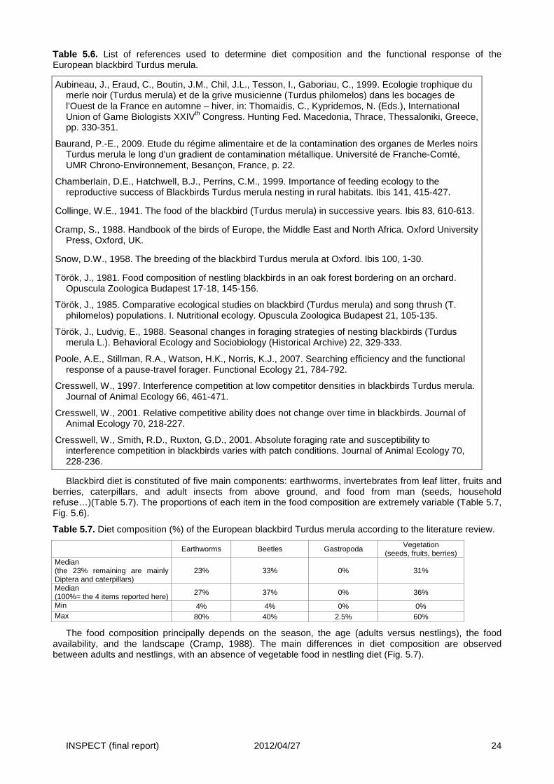
Data from a literature review and from INSPECT have been collected on the diet and habitat of two new target species (the European blackbird Turdus merula, the common kestrel Falco tinnunculus). From the literature, it has been shown that blackbird diet is constituted of five main components: earthworms, invertebrates from leaf litter, fruits and berries, caterpillars, and adult insects from above ground, and food from man (seeds, household refuse…). The proportions of each item in the food composition are extremely variable. The food composition principally depends on the season, the age (adults versus nestlings), the food availability, and the landscape. The diet of suburban blackbirds (as in the Metaleurop Nord smelter area) is
INSPECT (final report) 2012/04/27 3
dominated by earthworms. Therefore, we conclude that earthworms (which represent 4 to 80% of the food) and invertebrates from leaf litter (which represent 30 to 40% of the food) are the main diet items of the blackbird and must be included as diet items in BERISP-DSS. Data from the STARTT programme were in agreement with the literature review, and showed that blackbirds mainly fed on earthworms (56 %) and insects (26 %), while vegetation and other items such as spiders, myriapods, or slugs represented 4 and 14 %, respectively, of the total diet weights. The diet was influenced by habitat. Globally, we obtained a gradient from diet composed mostly by earthworms versus diet composed mainly by insects or other items. Vegetation amount poorly varied among individuals and were not related to a particular habitat. Earthworms in the diet increased notably with woodland with understory and short grass, while consumption of insects and other items seemed to be dependent on the presence of woodland without understory, urban areas, hedgerows/copses and water. The influence of tall grass and shrubs is not clear, both earthworm and other items being associated with the presence of these habitats. These data were used to determine values introduced in the tables of BERISP-DSS that concern habitat-related diet preferences. From the literature, a diameter of home-range of 56 m was retained for the blackbird, which corresponds to the diameter of a 2455 m2 circular home-range. The diet of the common kestrel is mainly composed of herbivorous voles of Microtus species (about 50 to 96% of the diet reported in cited references). Other small mammals (shrews of genus Crocidura and Sorex, wild mice of genus Apodemus, Micromys and Mus, and bank voles Myodes glareolus) constitute additional preys, notably in case of low densities of Microtus voles. Beetles are eaten in extremely low proportion in comparison to small mammals (0 to 10%). Passerine birds can be predated during certain seasons (winter principally), and in some particular cases (big cities and certain sites in western Scandinavia) constitute a large part of the food (0 to 41%). Small mammals are consumed all over the year contrarily to birds and beetles. Based on literature data, we propose to use a diameter of home-range of 1596 m in BERISP-DSS, which corresponds to the diameter of a 2 km2 circular home-range. Rejection pellets were sampled during the STARTT programme nearby common kestrel nests in the surroundings of the ancient Metaleurop smelter. Rests were searched in 12 pellets, and could be identified in only 6 pellets. Small mammals were found, with among them only voles of Microtus species (M. arvalis and M. agrestis). Rests of insects were also found in 2 pellets. Data on prey availability for the common kestrel and toxicological reference values for passerine and raptor birds were also implemented in BERISP-DSS.
In order to implement large grazers into the DSS, it is necessary to collect data and it is essential to establish scientific founded relationships between soil contamination and different types of vegetation, taking into account soil characteristics such as pH, organic content and clay content. To make the DSS generic, it is essential that those relationships are established for different types of soil and different plant species. In a first phase, we searched in literature to find studies on the relationships between metals in soils and in vegetation that take into account the soil characteristics. In a second phase, we sampled soil, grasses and nettles at different sites in Flanders to establish these relationships and to provide multiple linear models that take into account soil characteristics. Besides measuring total metal levels in the soil we also measured exchangeable metal fractions. Metal accumulation appeared to be similar in grasses and Urtica dioica except for Pb. Urtica dioica accumulated more than grasses. No significant difference between forest and grassland sites in metal content was observed. However, at Fort 8, one of the more polluted sites, the forest sites showed a significantly higher metal concentration than the grassland sites. Even though Pb generally occurs in organic complexes and is thus not available for uptake by vegetation, significant models could be constructed. Other metals that showed significant modeling potential were As in nettle and Cd, Cu, and Zn in grass. These models were used to optimize the grazers module in BERISP-DSS.
The possible effects of spatial metal distribution, soil characteristics, vegetation type, seasonal variation, habitat, and vegetation use in the Hageven-Plateaux reserve, were investigated on the metal exposure of grazers. Metal concentrations in soil, vegetation and blood, hair and feces of free ranging Galloway cows (Bos taurus) were measured. The metal exposure was measured by observing the habitat use, vegetation selection, and foraging behavior of the cows and measuring the metal concentrations in their food. Positive linear relations were found between metal concentrations in soil and vegetation, for Cd, As and Co. Bioaccumulation of metals in vegetation was mostly affected by pH, followed by organic matter content, and less by clay fraction. Vegetation use of the Galloways differed between seasons, the habitat and vegetation use was different between herds. There was also a significant difference in metal concentrations between the different vegetation types. The differences in vegetation use and spatial variation on metal concentrations resulted in a different metal exposure pattern among the two herds. For some metals these differences in metal exposure resulted in differences in metal concentrations in blood, hair, and feces of the Galloways. Some results of this study were used to implement the grazers module in BERISP-DSS.
Both the manual for users and the website have been updated. Three new metals (Cu, Pb, Zn) have also been added in the DSS using transfer equations from data from previous and the current INSPECT programmes. According to the communication plan of the programme, two presentations of the DSS were done in stakeholders meetings (one in Mechelen, Belgium, one in Gouda, The Netherlands) and eight talks were presented in scientific congresses. Four articles presenting some parts of the programme were published in international scientific journals, and the DSS was presented in an article in Environnement Magazine, a French journal for professionals of the environment (industry, national agencies, administrations…).
INSPECT (final report) 2012/04/27 4
Samenvatting
De centrale doelstelling van dit programma is het beter integreren van risico’s van bodemverontreiniging in landinrichting en in ruimtelijke planningsprocessen om maatregelen te nemen die de risico’s voor mens en natuur zo efficiënt mogelijk beperken. Om dit doel te bereiken werd binnen dit project een bestaand beslissingssysteem (Decison Support System of DSS), BERISP genaamd (www.berisp.org), gevalideerd en uitgebreid en was het de bedoeling om dit te verspreiden binnen de wetenschappelijke gemeenschap en de stakeholders die betrokken zijn bij het beheer van gecontamineerde bodems. De BERISP-DSS werd recent ontwikkeld om het risico van contaminanten voor wilde dieren, grote grazers en kinderen in te schatten op een ruimtelijk expliciete wijze. De DSS kan op verschillende schalen worden gebruikt, gaande van zeer gedetailleerde plaats-specifieke evaluaties tot grote gebieden. De DSS is voornamelijk bedoeld om de risico’s van duffuse bodemverontreiniging in te schatten en integreert de informatie van de concentraties aan stoffen met de bodemkarakteristieken, het habitattype en de ecologische kenmerken van de studiesoort die in het habitat voorkomt. De eerste deeldoelstelling is de initiële BERISP-DSS verder te ontwikkelen tot een breder toepasbaar instrument. Oorspronkelijk was de BERISP-DSS ontwikkeld voor één case-study; het overstromingsgebied ‘de Afferdensche en Deetsche Waarden’ voor slechts één metaal, met name cadmium en één soort de steenuil (Athene noctua). Om de DSS te kunnen uitbreiden werden bestaande en nieuwe data verzameld van twee verschillende metaal-verontreinigde gebieden: Het grensoverschrijdend (België-Nederland) ‘Hageven-Plateaux’ natuurreservaat en ‘Metal-Europe Nord’ in noord Frankrijk. Beide gebieden zijn verontreinigd door Zn/Pb metaalverwerkende bedrijven. Drie nieuwe metalen (Cu, Pb en Zn) werden toegevoeds aan de DSS evenals twee nieuwe doelsoorten, de merel en grote grazers (Galloway koeien).
Het Metal-Europe gebied werd succesvol ingebracht in de DSS. De habitatkaart werd geactualiseerd na veldstudies uitgevoerd binnen het INSPECT-programma en additionele bodemmonsterpunten, behorende tot de databank van het Laboratoire Génie Civil et géo-Environnement (LGCgE, Lille, France), werden toegevoegd met de toestemming van Francis Douay (verantwoordelijke voor de LGCgE bodemdatabank). Voor het Hageven-Plateaux werden op dezelfde manier de habitat-, de bodemkarakteristieken- en de verontreinigingskaarten ingevoegd in de software.Voor de Metal-Europe site werden de Cd-concentraties in kleine zoogdieren, voorspeld door BERISP, vergeleken met geaccumuleerde gehaltes gemeten in het kader van andere onderzoeksprogramma’s uitgevoerd in Metal-Europe, namelijk STARTT en PHYTENER. Uit deze vergelijking bleek dat de cadmiumgehaltes door BERISP werden overschat voor spitsmuizen en onderschat voor herbivore woelmuizen. Voor spitsmuizen werden significante correlaties gevonden tussen voorspelde en effectief gemeten concentraties en ondanks hogere voorspelde waarden waren de gehaltes in dezelfde grootte-orde. Doordat er een grote variatie in bioaccumualtie van Cd was en doordat verschillende soorten spitsmuizen van verschillende leeftijden (leeftijd is een belangrijke factor die Cd opname beïnvloedt) werden bemonsterd, bleek de voorspelling van Cd-accumulatie globaal genomen betrouwbaar voor spitsmuizen. Voor woelmuizen bleek de correlatie tussen voorspelde en gemeten waarden eveneens sterk maar waren de voorspelde waarden 4 tot 5 maal lager. Om deze inconsistentie verder te onderzoeken werden de cadmiumgehaltes gemeten in grassoorten van Metal-Europe vergeleken met voorspelde gehaltes gebruikmakend van de regressievergelijkingen tussen bodem en vegetatie uit BERISP. Dit bleek goed overeen te stemmen; een sterke correlatie werd gevonden en gemodelleerde en gemeten gehaltes waren niet significant verschillend.Vervolgens werden de cadmiumgehaltes in de maaginhoud van kleine zoogdieren uit Metaluerope gemeten en vergeleken met de voorspelde vegetatiewaardes. Opnieuw werd een sterke correlatie gevonden maar de voorspelde waardes waren significant lager dan de gemeten maaginhouden (tot vijfmaal lager). Een gelijkaardige vergelijking werd uitgevoerd voor spitsmuizen; hier werden de met BERISP voorspelde waarden in regenwormen vergeleken met gehaltes in maaginhoud van spitsmuizen, waaruit bleek dat de gehaltes zeer goed overeenkwamen. Op basis van deze studie werd besloten om de data rond dieet van kleine zoogdieren, gebruikt in het BERISP-programma aan te passen. Een literatuuronderzoek werd uitgevoerd om (1) de definitie van het dieet van Microtus-soorten en spitsmuissoorten gegeten door steenuil en torenvalk verbeteren en (2) het bepalen van het dieet van twee nieuwe kleine zoogdiersoorten, namelijk de bosmuis (Apodemus sylvaticus) en de rosse woelmuis (Myodes glareolus) zodat deze kunnen worden toegevoegd als nieuwe soorten in BERISP.
Gebruikmakend van een literatuuronderzoek en van metingen binnen INSPECT werden twee nieuwe doelsoorten aan de DSS toegevoegd, de merel (Turdus merula) en de torenvalk (Falco tinunculus). Uit de literatuur bleek dat het dieet van de merel bestaat uit verschillende componenten; regenwormen, bodeminvertebraten, bessen, rupsen, adulte insecten en menselijk voedsel (etensresten en zaden). Het relatief aandeel van elk van deze voedselitems is zeer variabel en hangt af van het seizoen, de leeftijd van de vogels en het landschap. Het dieet van sub-urbane merels (zoals in Metal-Europe) wordt gedomineerd door regenwormen. We konden besluiten dat regenwormen en bodeminvertebraten de belangrijkste dieet items waren en toegevoegd moeten worden aan de BERISP. Ook de data van het STARTT programma kwamen overeen met de literatuur en toonden dat merels zich voornamelijk voeden met regenwormen (56 %) en insecten (26%) terwijl andere voedselitems zoals veelpotigen, spinnen en slakken slechts maximaal 14 % van het dieet uitmaken. Het dieet bleek beïnvloed te zijn door het habitat en er werd een gradiënt waargenomen van bijna uitsluitend regenwormen tot voornamelijk insecten of andere items. Plantaardig
INSPECT (final report) 2012/04/27 5
voedsel varieerde slechts weinig en was niet gerelateerd aan habitat. Het aandeel aan regenwormen nam vooral toe in bos met ondergroei en kort gras terwijl in bos zonder ondergroei en in urbane gebieden voornamelijk insecten en andere items werden gegeten. De invloed van lang gras en struiken was niet duidelijk.
Het dieet van de torenvalk bestaat voornamelijk uit herbivore woelmuizen (50-96 %). Andere kleine zoogdieren die worden gegeten zijn spitsmuizen, bosmuizen en huismuizen. Kevers werden in zeer kleine hoeveelheden gegeten (0-10 %). In sommige seizoenen worden zangvogels gegeten en kunnen in bepaalde gevallen (bvb steden) een belangrijk deel uitmaken van het dieet van torenvalken (tot 41%). Voor zowel merel als torenvalk werden home-ranges vastgesteld die opgenomen werden in BERISP.
Om grazers op te nemen in de DSS, is het nodig data te collecteren die essientieel zijn om relaties te leggen tussen de metaalgehaltes in de bodem met die in verschillende vegetatietypes, waarbij rekening dient te worden gehouden met bodemkarakteristieken zoals pH, kleigehalte en organisch materiaal. Om de DSS generiek te kunnen maken was het belangrijk om deze relaties te ontwikkelen voor een brede waaier aan bodemtypes. In een eerste fase werd een grondige literatuurstudie uitgevoerd naar dergelijke bodem-plant relaties die ook met bodemkarakteristieken rekening houden. Vermits er slechts een beperkt aantal studies werden gevonden in de literauur, werden additioneel op een groot aantal plaatsen in Vlaanderen en Frankrijk metalen gemeten in bodemstalen en in zowel grassen als netels. Simultaan werden van elke bodem de bodemkarakteristieken gemeten en multipele regressie-modellen opgesteld die de relatie tussen bodemverontreiniging en geaccumuleerde gehaltes moeten kunnen beschrijven. Voor alle metalen behalve lood bleken de gehaltes in grassen en netels sterk overeen te komen. Netels (Urtica dioica) accumuleerden significant meer Pb dan grassen. Er werd geen verschil gevonden in relaties tussen verschillende habitats (bos en grasland). Op één plaats echter, Fort 8 in Hoboken, vlak bij een metaalverwerkend bedrijf waren de gehaltes in grasland significant hoger dan in het bos. Hoewel lood meestal in organische complexen voorkomt en weinig biobeschikbaar is voor planten konden toch modellen ontwikkeld worden die een significante relatie aantoonden. Andere metalen waarvoor relatief goede modellen konden worden opgesteld waren As voor netels en Cd, Cu en Zn voor grassen. Deze modellen werden gebruikt om de ‘grazers module’ in BERISP te optimaliseren. De mogelijke effecten van spatiale variatie in metaaldistributie, bodemkarakteristieken, vegetatietype, seizoen, habitat en vegetatiegebruik op de metaalblootstelling van grazers werd onderzocht in het Hageven-Plateaux reservaat. Metaalgehaltes werden gemeten in bodem, vegetatie, bloed, haar en uitwerpselen van vrij rondlopende Galloway koeien. De blootstelling werd bovendien bepaald door het graasgedrag van de koeien te volgen waarbij gelet werd op het type vegetatie dat gegeten werd. Het vegetatiegebruik van de Galloways verschilde sterk per seizoen en er werden verschillen gevonden tussen verschillende kuddes. De gegevens over graasgedrag, concentraties in bodem en vegetatietype werden ingebracht in BERISP om de grazers module te optimaliseren.
Gebaseerd op al de nieuwe ingevoegde data werden de handleiding en de website (www.berisp.be) geactualiseerd. Er werden, zoals opgenomen in het communicatieplan, twee presentaties ivm de DSS gegeven voor stakeholders; één in Mechelen (België) en één in Goude (Nederland) en 8 voordrachten werden gehouden op internationale symposia. In totaal werden er vier wetenschappelijke artikels gepubliceerd in internationale tijdschriften and werd de DSS voorgesteld in Environement Magazine een Frans tijdschrift voor professionele beheerders (zowel overheid als industrie).
INSPECT (final report) 2012/04/27 6
Acknowledgement The authors thank ADEME, OVAM, and SKB for funding the INSPECT research programme in the
framework of the 2nd SNOWMAN Network call for research proposals. Hanny Verbakel is gratefully acknowledged for her help. Cécile Grand and Nadine Dueso (ADEME), Simon Molenaar (SKB), Sofie van den Bulck and Filip Collet (OVAM), are also gratefully acknowledged for fruitful scientific discussions.
INSPECT (final report) 2012/04/27 7
Table of content 1 Background ........................................ .................................................................................... 9
2 Aims of the project ............................... ............................................................................... 10
3 Results WP1 ....................................... .................................................................................. 12
3.1 Report on kick-off meeting, annual progress report (midterm) and final project report to Snowman secretariat ................................................................................................................. 12
3.2 Synthesis on WP1 ....................................................................................................... 12
4 Results WP2 ....................................... .................................................................................. 13
4.1 Species and contaminants to be included in the DSS .................................................. 13
4.1.1 Species ....................................................................................................................... 13
4.1.2 Case studies ............................................................................................................... 13
4.1.3 Pollutants .................................................................................................................... 13
4.2 Communication plan .................................................................................................... 13
4.3 Synthesis on WP2 ....................................................................................................... 15
5 Results WP3 Case study “Metaleurop” ............... ............................................................... 16
5.1 Delivery of data essential for the validation or the optimisation of the modelling of small mammal contaminant burdens .................................................................................................. 16
5.1.1 Prediction of Cd body burdens in small mammals using BERISP-DSS and comparison with measured concentrations over Metaleurop area ........................................................... 16
5.1.2 Prediction of Cd body burdens in small mammals: analyses of metal concentrations in the food of small mammals .................................................................................................. 19
5.1.3 Prediction of Cd body burdens in small mammals: proposal for improvements ........... 21
5.2 Delivery of data essential for the development of a possible “blackbird” module in BERISP-DSS (WP5).................................................................................................................. 23
5.2.1 Literature review on blackbird and common kestrel foraging and spatial behaviour .... 23
5.2.2 Analyses of the diet of blackbirds and common kestrels from the Metaleurop area ..... 27
5.2.3 Data on prey availability .............................................................................................. 29
5.2.4 Toxic thresholds for passerine birds and raptors ......................................................... 33
5.3 Presentation of the results to possible end users in combination with workpackages 2 and 4 .................................................................................................................................... 34
5.4 Publication of the results in peer reviewed journals in combination with workpackages 2 and 4 .................................................................................................................................... 34
5.5 Risk assessment for the little owl with the current version of the DSS ......................... 35
5.6 Validation of prediction of Cd small mammal body burdens by the new BERISP-DSS version and risk assessment for the little owl ............................................................................. 36
5.7 Risk assessment for the blackbird and the common kestrel using the new version of BERISP-DSS, and validation of prediction for the blackbird....................................................... 39
5.8 Synthesis on WP3 ....................................................................................................... 39
6 Results WP4 Case Study “Campine region and Valley o f the River Dommel” ................ 40
6.1 Delivery of data essential for the optimization of the grazer module in the DSS .......... 40
6.1.1 Introduction ................................................................................................................. 40
6.1.2 Materials and Methods ................................................................................................ 40
6.1.3 Results and discussion ............................................................................................... 41
6.1.4 Conclusion .................................................................................................................. 42
6.2 Report on the risks of the soil contamination in the study area .................................... 42
6.2.1 Introduction ................................................................................................................. 42
6.2.2 Materials and methods ................................................................................................ 43
6.2.3 Results and discussion ............................................................................................... 46
6.3 Presentation of the results to possible end users in combination with workpackages 2 and 3 .................................................................................................................................... 71
6.4 Publication of the results in peer reviewed journals in combination with workpackages 2 and 3 .................................................................................................................................... 71
6.5 Synthesis on WP4 ....................................................................................................... 71
INSPECT (final report) 2012/04/27 8
7 Progress in WP5 DSS development ................... ................................................................ 72
7.1 Development of the BERISP-DSS ............................................................................... 72
7.2 Case studies incorporated in the DSS ......................................................................... 73
7.3 Updated manual for the new developed DSS .............................................................. 75
7.4 Synthesis on WP5 ....................................................................................................... 75
8 Application of results, conclusion and perspectives ........................................................ 76
9 References ........................................ ................................................................................... 76
INSPECT (final report) 2012/04/27 9
1 Background
Europe is densely populated, with increasing demands on land use. Often, development of areas is restricted by (local) contamination of the soils in the area of concern, which are a legacy of the past. A major service of soils is to provide suitable substratum for the development of (semi-)natural ecosystems, and for recreational use. This service is of great importance in both economic values, as well as in intrinsic values in case of natural development. Different policy fields at both the EU and the national level regarding soil contaminants are related to these soil services. Since space is scarce in Europe, it is of importance that contaminated, derelict areas can be redeveloped and upgraded into areas with soils that can sustain people to live, recreate or where natural values can be improved. Although scientifically state of the art tools and methods have been developed to assess environmental risks of contaminants, stakeholders cannot easily participate in such assessments. Furthermore results of current methods lack spatial information, which limits their use in spatial planning processes. In a recent project a spatially explicit decision support system (BERISP-DSS) has been developed in order to overcome this (see www.berisp.org). This DSS incorporates information on soil contamination, habitat configuration and other case/site specific information to assess risks of soil contaminants to wildlife, grazers and small children in a spatially explicit way. The user-interface of the DSS has been designed with stakeholders so they can use the DSS after an only short introduction. Results are presented in maps for easy integration in decision making process in spatial planning.
However, for a wider application of the BERISP-DSS, it is needed to: � Further develop the DSS so it can target more contaminants and animal species of concern. � Communicate the DSS to a wider audience of stakeholders, making use of case studies that can be
conducted.
In the former project, the framework of the DSS has been developed, in combination with a user friendly interface. It includes heavy metals, and the receptors included are the little owl, large grazers and small children. For a wider applicability it is needed to address other types of soil contaminants like organic contaminants and to include other receptor species. Furthermore, case studies are needed, which can be used to validate the DSS, and to illustrate the applicability to a wider audience. Both actions will increase the range of applicability of the DSS considerably, and this will offer opportunities to truly integrate environmental risk assessment of contaminants into spatial planning processes. In addition to this it should be noted that the DSS is focused on solutions of problems and not so much on just defining them. This will more likely enable the development of nature areas and recreational areas in the vicinity of urban regions on more or less contaminated area.
Work plan
The project comprises 5 work packages: management and coordination (WP1); communication and dissemination (WP2); two case studies (WP3 and 4); development of the DSS (WP5). For detailed description of the WPs see later, here we will present a brief overview of the main activities of the proposal on communication, case studies and DSS development and the interactions.
Communication The final aim of the project is to provide a DSS that can be implemented by various stakeholders.
Therefore, communication is essential. In different ways different stakeholders in spatial planning or people otherwise interested will be contacted through reports, presentations, and a final work-shop. The website on the DSS will be actualized. The web-site includes a demo DSS based on pre-set scenario calculations, with which people can play to get familiar with. Specific scientific meeting and workshop presentations will be delivered of the concepts and feasibility of the approach. This will ensure the quality assurance of the scientific part of the project. All partners are involved. The knowledge and applicability of the final DSS will be spread to the scientific community, through scientific papers and presentations.
DSS-development The framework of the BERISP-DSS has been developed technically by Alterra, and all sources are
available for this project. Based upon this framework new models can be integrated relatively easily. The choice of additional contaminants and ecological receptors will be defined in cooperation with stakeholders at the kick-off meeting. This ensures a further development with high relevance for application. The innovative part of the further development is to integrate ecological traits and properties of additional species with food web dynamics, habitat specifics and soil properties. The specific modelling will be quite challenging, including (foraging) ecology, spatial exploitation models, and bioaccumulation dynamics. Currently, several manuscripts on these issues resulting from the former project are being submitted, but demanding information gaps still exists. Issues that need to be resolved are on physiokinetic based modelling of uptake of other contaminants by organisms, spatially explicit exploitation modelling of selected species and the assessment of functional responses and other ecological relationships. Furthermore, the interaction with the case studies allows validating the modelling, which is generally not performed in case of
INSPECT (final report) 2012/04/27 10
spatially explicit modelling.
Case studies The first case study (WP 3) site corresponds to the surroundings of the former “Metaleurop Nord” smelter
in France. Data are available on contaminant levels and characteristics of soil samples, in combination with concentrations in small mammals and blackbirds and samples. Additional samples of their respective food webs are ready to be analyzed within this SNOWMAN project.
A second case study (WP4) site is a trans boundary region between the Netherlands and Flanders. This region in the Campine is historically contaminated due to the presence of a zinc smelter. Soil data and data on grazers are present.
In order to validate and refine the DSS, additional data on those 2 sites (contaminants in items of the diet of species of concern for both sites (e.g. vegetation for cows in site 2), data on grazing behaviour of the cows…) have to be collected.
The data from both case studies will allow an extension of the DSS with several new wildlife species and grazers. Thanks to the established relationships in both case studies between soil contamination and biota (vegetation, invertebrates, mammals, birds and grazers) input is given to the DSS, making it more applicable in new areas.
2 Aims of the project
The overall objective of this programme is to better integrate environmental risk assessment of contaminants into land management and spatial planning processes in order to mitigate possible risks as efficiently as possible. To reach this goal, the operational objectives of this project are to validate and extend the use of a spatially explicit decision support system (DSS) named BERISP (www.berisp.org) and to spread it within the scientific community and stakeholders involved in the study and management of contaminated sites.
The detailed objectives are:
Objective 1: develop BERISP-DSS for a wider range of application in spatial planning processes,
Objective 2: perform case studies for validation and extension of the BERISP-DSS and for communication (objective 3),
Objective 3: communicate the BERISP-DSS to lay audience, stakeholders and the scientific community.
The programme comprises 5 work packages (including 2 case studies, Table 1): management and coordination (WP1); communication and dissemination (WP2); two case studies (WP3 and 4); development of the DSS (WP5).
The first case study (WP3) site corresponds to the surroundings of the former “Metaleurop Nord” smelter in France. Data are available on contaminant levels and characteristics of soil samples, in combination with concentrations in small mammals and blackbirds. Additional samples of their respective food webs were already available for analysis but complementary field sessions were planned within INSPECT.
A second case study (WP4) site is a trans-boundary region between the Netherlands and Flanders. This region in the Campine is historically contaminated due to the presence of a zinc smelter. Soil data and data on grazers were partly available at the beginning of the programme and, as for WP3, additional analyses of collected samples and more field samplings were planned.
Even if most of work packages are carried out by all partners in cooperation and are obviously not independent, it has been thought clearer and simpler to follow the same structure for the present report, which thus will be constituted by 5 parts, dedicated to the WP1, WP2, WP3, WP4 and WP5, respectively.
INSPECT (final report) 2012/04/27 11
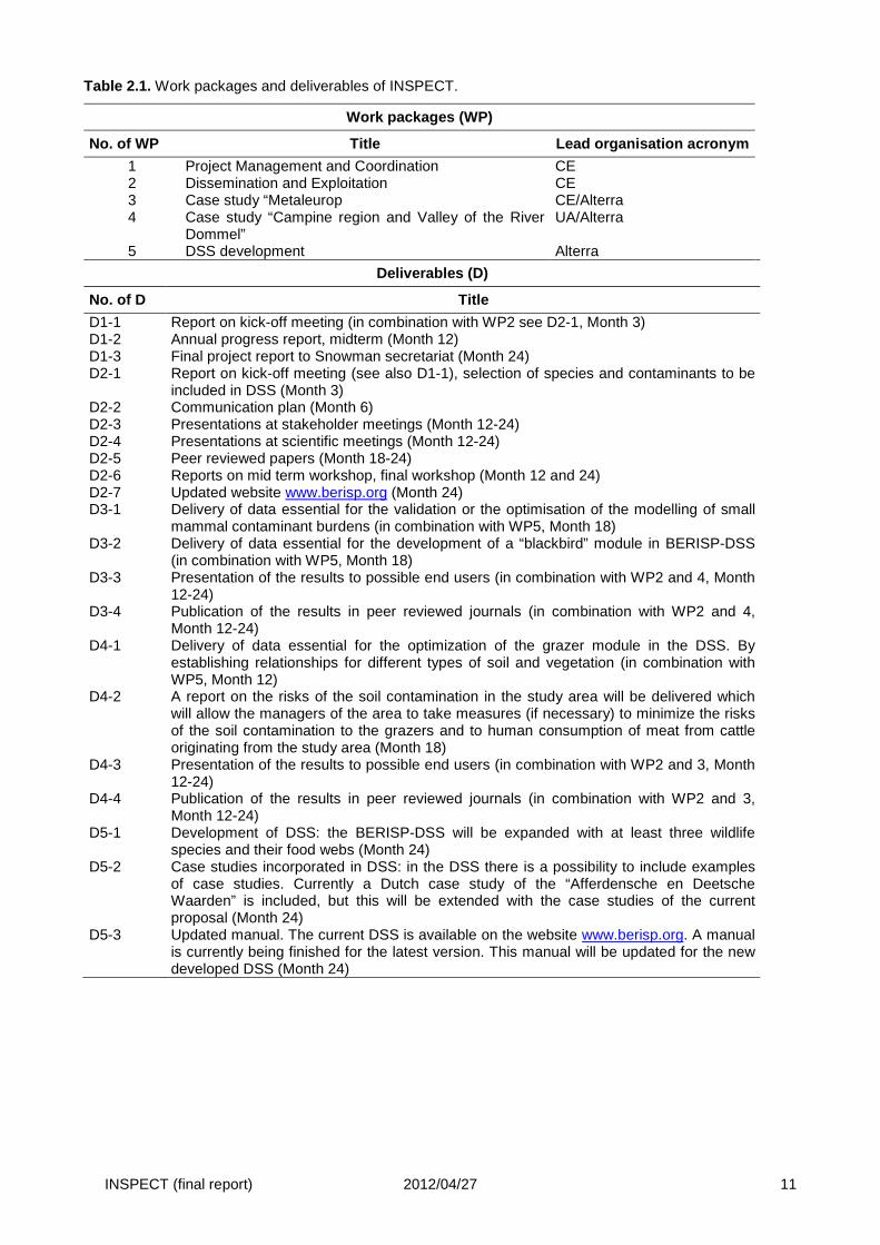
Table 2.1. Work packages and deliverables of INSPECT.
Work packages (WP)
No. of WP Title Lead organisation acronym
1 Project Management and Coordination CE 2 Dissemination and Exploitation CE 3 Case study “Metaleurop CE/Alterra 4 Case study “Campine region and Valley of the River
Dommel” UA/Alterra
5 DSS development Alterra
Deliverables (D)
No. of D Title
D1-1 Report on kick-off meeting (in combination with WP2 see D2-1, Month 3) D1-2 Annual progress report, midterm (Month 12) D1-3 Final project report to Snowman secretariat (Month 24) D2-1 Report on kick-off meeting (see also D1-1), selection of species and contaminants to be
included in DSS (Month 3) D2-2 Communication plan (Month 6) D2-3 Presentations at stakeholder meetings (Month 12-24) D2-4 Presentations at scientific meetings (Month 12-24) D2-5 Peer reviewed papers (Month 18-24) D2-6 Reports on mid term workshop, final workshop (Month 12 and 24) D2-7 Updated website www.berisp.org (Month 24) D3-1 Delivery of data essential for the validation or the optimisation of the modelling of small
mammal contaminant burdens (in combination with WP5, Month 18) D3-2 Delivery of data essential for the development of a “blackbird” module in BERISP-DSS
(in combination with WP5, Month 18) D3-3 Presentation of the results to possible end users (in combination with WP2 and 4, Month
12-24) D3-4 Publication of the results in peer reviewed journals (in combination with WP2 and 4,
Month 12-24) D4-1 Delivery of data essential for the optimization of the grazer module in the DSS. By
establishing relationships for different types of soil and vegetation (in combination with WP5, Month 12)
D4-2 A report on the risks of the soil contamination in the study area will be delivered which will allow the managers of the area to take measures (if necessary) to minimize the risks of the soil contamination to the grazers and to human consumption of meat from cattle originating from the study area (Month 18)
D4-3 Presentation of the results to possible end users (in combination with WP2 and 3, Month 12-24)
D4-4 Publication of the results in peer reviewed journals (in combination with WP2 and 3, Month 12-24)
D5-1 Development of DSS: the BERISP-DSS will be expanded with at least three wildlife species and their food webs (Month 24)
D5-2 Case studies incorporated in DSS: in the DSS there is a possibility to include examples of case studies. Currently a Dutch case study of the “Afferdensche en Deetsche Waarden” is included, but this will be extended with the case studies of the current proposal (Month 24)
D5-3 Updated manual. The current DSS is available on the website www.berisp.org. A manual is currently being finished for the latest version. This manual will be updated for the new developed DSS (Month 24)
INSPECT (final report) 2012/04/27 12
3 Results WP1
Following the actual beginning of the project in January 2010, constant communication between partners since this date has been going on and several meetings were organized in Vienna (official SNOWMAN kick-off meeting, February, 9th and 10th 2010), Antwerp (March, 2nd 2010), Sevilla (SETAC Europe meeting, May, 23rd to 27th 2010), Noyelles-Godault (where the Metaleurop Nord study site is located, June, 22nd 2010), Milan (SETAC Europe meeting, May, 15th to 19th 2011).
The INSPECT kick-off meeting was held on October, the 28th 2010 at Alterra, Wageningen, The Netherlands. Clémentine Fritsch was welcomed at Alterra during 3 months (September 5th to December 2nd), allowing daily exchanges and communications between the partners CE and Alterra.
Main results of the programme were presented at the mid-term SNOWMAN Call 2 meeting, held on November, the 8th and 9th at Paris, France.
A meeting was held in Besançon during December 2011 (14th to 16th December), allowing a last evaluation of the INSPECT programme results and perspectives.
3.1 Report on kick-off meeting, annual progress rep ort (midterm) and final project report to Snowman secretariat
The report on kick-off meeting (D1-1) and the annual progress report (midterm, D1-2) were provided to SNOWMAN secretariat.
The present report constitutes the contribution to the last deliverable D1-3 of WP1.
3.2 Synthesis on WP1
Deliverables (D)
No. of D Title Progress
D1-1 Report on kick-off meeting (in combination with WP2 see D2-1, Month 3) Done D1-2 Annual progress report, midterm (Month 12) Done D1-3 Final project report to Snowman secretariat (Month 24) Present
document
INSPECT (final report) 2012/04/27 13
4 Results WP2
4.1 Species and contaminants to be included in the DSS
4.1.1 Species At the beginning of the programme, small mammals (as major preys in the diet of the target species of the
BERISP-DSS, i.e. the little owl Athene noctua), large grazers (cows), and the common blackbird (Turdus merula) were the models to be studied within the framework of the INSPECT programme. Another species, the common kestrel (Falco tinnunculus), has been added because (i) this raptor, common and abundant in the Palearctic, may constitute a good model for many contaminated sites, and (ii) the species is present of the site of Metaleurop Nord while the absence of the little owl is suspected.
4.1.2 Case studies BERISP currently provides, for demonstration use only, a pre-installed example called “Afferdsche en
Deestsche Waarden”. This is a real floodplain in the Netherlands along the river Rhine, with contamination problems. The Metaleurop case study has been added in BERISP-DSS. This new case study illustrates a larger site than the floodplain of Afferdsche en Deestsche Waarden. The source and the range of contamination level (in the soils) are also different: while the plain is mainly contaminated by flooding of the Rhine river, Metaleurop surroundings were mainly contaminated by aerial deposits of pollutants coming from the chimneys of the former lead smelter of Metaleurop Nord (Douay et al., 2009)(Fritsch et al., 2010). A third case study included in BERISP-DSS is the “Hageven-Plateaux” or valley of the River Dommel situated in the North of Flanders and South of the Netherlands. It is a 555 ha large reserve existing of heath land, ponds and forests, which is situated at 1.5 km north of a zinc smelter which caused metal pollution in the region during the second half of last century. Finally, target species will be different (little owl and grazers in the plains, blackbirds and kestrels in Metaleurop), even if the DSS could run on every included species in every case study sites.
4.1.3 Pollutants Data allowing the inclusion of Cu, Zn, Pb, and PCBs have been collected during INSPECT. All metals
have been implemented in the new version of BERISP-DSS. For the latter contaminant, two new adequate transfer equations have been developed but work is still needed to implement this pollutant in the DSS.
4.2 Communication plan • Stakeholder meetings
o 2012. Stakeholder workshop at OVAM, Mechelen, 12 March 2012. At this workshop, the DSS was presented to stakeholders. The workshop was attended by 18 persons. The stakeholders could also “play” with the DSS in order to familiarise themselves with the program. One participant took along a new case study, which was used in the workshop.
o 2012. Stakeholder workshop 2012 SKB, Gouda, 14 March 2012. This was a workshop similar to the workshop at 12 March in Mechelen. This workshop attracted 21 participants, from consultancies to policy makers and environmental managers. In the morning the participants were introduced to the DSS, in the afternoon computers with the DSS were available for people to get to know the DSS.
• Scientific meetings
o 2010. van den Brink N., Bervoets L., Scheifler R. A tool for spatially explicit assessment of ecological risks of contaminants to wildlife (BERISP-DSS). Sustainable approaches to remediation of contaminated land in Europe, 8-10 June, Gent, Belgium.
o 2011. Fritsch C. Quels outils pour l’évaluation des risques pour les écosystèmes terrestres liés à des terrains contaminés? (“What tools to assess environmental risk on contaminated lands in terrestrial ecosystems?”). “Groupe ERE” meeting, 27-28 September, Paris, France. The main aim of this seminar was to promote the transfer of knowledge, tools and methods developed through several scientific research programmes to French end-users (French administrations (DREAL for instance), national public agencies (ADEME for instance), stakeholders, industrial and consultancy companies).
INSPECT (final report) 2012/04/27 14
o 2010. Roggeman S., Van Praet N., Bervoets L. Accumulation and effects of metals in a
metal polluted nature reserve with grazing cattle. 20th SETAC Europe meeting, 23-27 May, Seville, Spain.
o 2011. Scheifler R., Fritsch C., Raoul F., Cœurdassier M., Giraudoux P. Landscape ecotoxicology: state of the art and perspectives. IALE 8th World Congress, 18-23 August, Beijing, China.
o 2011. Fritsch C., Giraudoux P., Cœurdassier M., Raoul F., Scheifler R. Landscape modulates transfer and effects of metallic trace elements in small mammals. IALE 8th World Congress, 18-23 August, Beijing, China.
o 2011. van den Brink N., Bervoets L., Baveco H., Fritsch C., Scheifler R. Circumnavigating risks of environmental contamination in spatial planning by the use of spatially explicit risk assessment procedures. IALE 8th World Congress, 18-23 August, Beijing, China.
o 2011. Fritsch C., Giraudoux P., Coeurdassier M., Raoul F., Vaniscotte A., Scheifler R. Le paysage module le transfert et les effets de polluants métalliques chez les micromammifères. 4ème Séminaire d’Ecotoxicologie de l’INRA, 7-9 November, Saint-Lager, France.
o A session entitled “Landscape ecotoxicology and spatially explicit risk assessment: from field data to modeling and regulatory implementation” was proposed to the organizing committee of the SETAC Europe 22nd Annual Meeting / 6th SETAC World Congress to be held in Berlin (Germany), 20-24 May 2012. The session was proposed by Andreas Focks (Alterra, Wageningen, The Netherlands), Mira Kattwinkel (UFZ, Leipzig, Germany) and Clémentine Fritsch (Chrono-environnement, Besançon, France). The session has been accepted but merged with two other session proposals dealing with similar topics. The final title of the session is “Landscape ecotoxicology and spatially explicit risk assessment”, with Andreas Focks (Alterra, Wageningen, The Netherlands), Ben Kefford (UTS, Sydney, Australia) and Ralf Schaefer (University Koblenz Landau, Landau, Germany) as co-chairs. The presentation cited hereafter has been presented in this session.
o 2012. van den Brink N.W., Fritsch C., Roggeman S., de Winter W., Baveco H., Scheifler R., Bervoets L. Accumulation of trace metals in a complex world, validation of a spatially explicit model: BERISP. 6th SETAC World Congress / SETAC Europe 22nd Annual Meeting, 20-24 May, Berlin, Germany.
• Website
The website (www.berisp.org) has been updated.
• Scientific articles (except the first one, see below, all these articles explicitly mention the INSPECT programme and SNOWMAN Call 2 funding)
o van den Brink, N., Lammertsma, D., Dimmers, W., Boerwinkel, M.-C., van der Hout, A., 2010. Effects of soil properties on food web accumulation of heavy metals to the wood mouse (Apodemus sylvaticus). Environmental Pollution, 158: 245-251. This article is based on work and data funded by INTERREG III and supports the development of the BERISP-DSS.
o van den Brink, N., Lammertsma, D., Dimmers, W., Boerwinkel, M.-C. 2011. Cadmium accumulation in small mammals: species traits, soil properties, and spatial habitat use. Environmental Science & Technology, 45: 7497-7502.
o Cœurdassier M., Fritsch C., Faivre B., Crini N., Scheifler R. 2012. Partitioning of Cd and Pb in the blood of European blackbirds (Turdus merula) from a smelter contaminated site and use for biomonitoring. Chemosphere, 87: 1368-1373.
o Fritsch C., Cœurdassier M., Faivre B., Giraudoux P., van den Brink N.W., Scheifler R. 2012. Influence of landscape composition and diversity on contaminant flux in terrestrial food webs: a case study of trace metal transfer to European blackbirds Turdus merula. The Science of the Total Environment, 432: 275-287.
o Roggeman S., van den Brink N., Van Praet N., Blust R., Bervoets L. 2013. Metal exposure and accumulation patterns in free-range cows (Bos Taurus) in a contaminated natural area: Influence of spatial and social behavior. Environmental Pollution, 172: 186-199.
INSPECT (final report) 2012/04/27 15
o van den Brink N., Fritsch C., Roggeman S., de Winter W., Baveco H., Bervoets L., Scheifler R. Accumulation of heavy metals in a complex world, validation of a spatially explicit model: BERISP. In preparation.
o Boshoff M., Blust R., Bervoets L. Effect of soil characteristics on the transfer of metals from soil to two plant species. In preparation.
o Boshoff M. Blust R., Bervoets L. Metal accumulation in a simplified terrestrial food chain along a metal pollution gradient. In preparation.
• Articles in stakeholder journals
o Article published (copy provided in attached file) in the January / February 2012 issue of Environnement Magazine. Environnement Magazine is the most spread journal dealing with the environment in France, and is intended for professionals from this economic sector.
4.3 Synthesis on WP2
Deliverables (D)
No. of D Title Progress
D2-1 Report on kick off meeting (see also D1-1), selection of species and contaminants to be included in DSS (Month 3)
Done
D2-2 Communication plan (Month 6) Done D2-3 Presentations at stakeholder meetings (Month 12-24) Done D2-4 Presentations at scientific meetings (Month 12-24) Done D2-5 Peer reviewed papers (Month 18-24) Done D2-6 Reports on mid-term workshop, final workshop (Month 12 and 24) Done D2-7 Updated website www.berisp.org (Month 24) Done
INSPECT (final report) 2012/04/27 16
5 Results WP3 Case study “Metaleurop”
5.1 Delivery of data essential for the validation o r the optimisation of the modelling of small mammal conta minant burdens
5.1.1 Prediction of Cd body burdens in small mammal s using BERISP-DSS and comparison with measured concentrations ove r Metaleurop area
It was decided at the INSPECT kick-off meeting to include the “Metaleurop” case study as an example in BERISP-DSS. The insertion of Metaleurop maps and data was successfully achieved and risk can now be calculated on the little owl in this area. Including the Metaleurop case in BERISP-DSS moreover constitutes a first essential step to validate, and to optimize if relevant, the modelling of small mammal contaminant burdens.
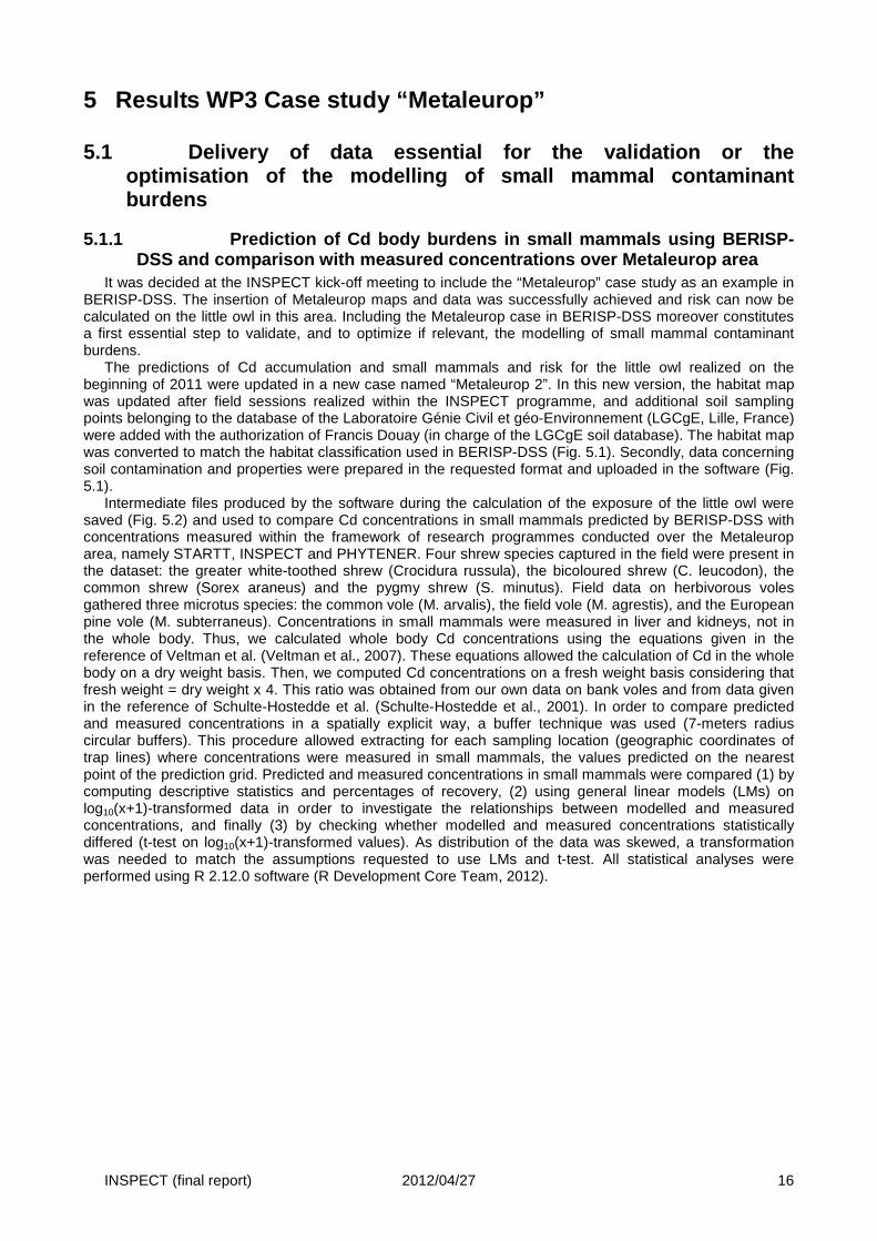
The predictions of Cd accumulation and small mammals and risk for the little owl realized on the beginning of 2011 were updated in a new case named “Metaleurop 2”. In this new version, the habitat map was updated after field sessions realized within the INSPECT programme, and additional soil sampling points belonging to the database of the Laboratoire Génie Civil et géo-Environnement (LGCgE, Lille, France) were added with the authorization of Francis Douay (in charge of the LGCgE soil database). The habitat map was converted to match the habitat classification used in BERISP-DSS (Fig. 5.1). Secondly, data concerning soil contamination and properties were prepared in the requested format and uploaded in the software (Fig. 5.1).
Intermediate files produced by the software during the calculation of the exposure of the little owl were saved (Fig. 5.2) and used to compare Cd concentrations in small mammals predicted by BERISP-DSS with concentrations measured within the framework of research programmes conducted over the Metaleurop area, namely STARTT, INSPECT and PHYTENER. Four shrew species captured in the field were present in the dataset: the greater white-toothed shrew (Crocidura russula), the bicoloured shrew (C. leucodon), the common shrew (Sorex araneus) and the pygmy shrew (S. minutus). Field data on herbivorous voles gathered three microtus species: the common vole (M. arvalis), the field vole (M. agrestis), and the European pine vole (M. subterraneus). Concentrations in small mammals were measured in liver and kidneys, not in the whole body. Thus, we calculated whole body Cd concentrations using the equations given in the reference of Veltman et al. (Veltman et al., 2007). These equations allowed the calculation of Cd in the whole body on a dry weight basis. Then, we computed Cd concentrations on a fresh weight basis considering that fresh weight = dry weight x 4. This ratio was obtained from our own data on bank voles and from data given in the reference of Schulte-Hostedde et al. (Schulte-Hostedde et al., 2001). In order to compare predicted and measured concentrations in a spatially explicit way, a buffer technique was used (7-meters radius circular buffers). This procedure allowed extracting for each sampling location (geographic coordinates of trap lines) where concentrations were measured in small mammals, the values predicted on the nearest point of the prediction grid. Predicted and measured concentrations in small mammals were compared (1) by computing descriptive statistics and percentages of recovery, (2) using general linear models (LMs) on log10(x+1)-transformed data in order to investigate the relationships between modelled and measured concentrations, and finally (3) by checking whether modelled and measured concentrations statistically differed (t-test on log10(x+1)-transformed values). As distribution of the data was skewed, a transformation was needed to match the assumptions requested to use LMs and t-test. All statistical analyses were performed using R 2.12.0 software (R Development Core Team, 2012).
INSPECT (final report) 2012/04/27 17
Figure 5.1. Input of data of “Metaleurop study case” in BERISP-DSS. Creation of base scenario uploading habitat map, contaminant maps and maps of soil properties.
Clay(%)
OM(%)
Habitat map
Cadmium(ppm DW)
Contaminants
pH
Soil properties
Lead(ppm DW)
Zinc(ppm DW)
INSPECT (final report) 2012/04/27 18
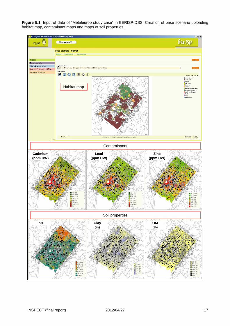
Figure 5.2. Maps of Cd concentrations predicted by BERISP-DSS in shrews (left panel) and in voles (right panel). Maps were built using data from intermediate ASCII files produced by the software.
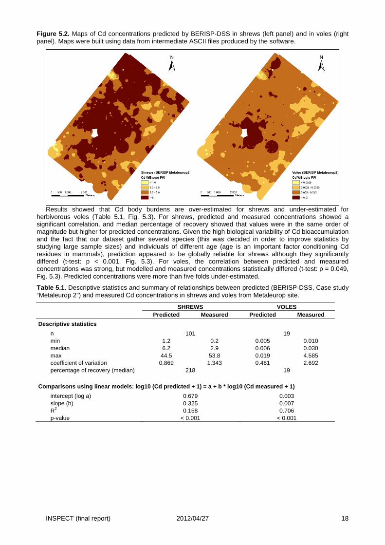
Results showed that Cd body burdens are over-estimated for shrews and under-estimated for herbivorous voles (Table 5.1, Fig. 5.3). For shrews, predicted and measured concentrations showed a significant correlation, and median percentage of recovery showed that values were in the same order of magnitude but higher for predicted concentrations. Given the high biological variability of Cd bioaccumulation and the fact that our dataset gather several species (this was decided in order to improve statistics by studying large sample sizes) and individuals of different age (age is an important factor conditioning Cd residues in mammals), prediction appeared to be globally reliable for shrews although they significantly differed (t-test: p < 0.001, Fig. 5.3). For voles, the correlation between predicted and measured concentrations was strong, but modelled and measured concentrations statistically differed (t-test: p = 0.049, Fig. 5.3). Predicted concentrations were more than five folds under-estimated.
Table 5.1. Descriptive statistics and summary of relationships between predicted (BERISP-DSS, Case study “Metaleurop 2”) and measured Cd concentrations in shrews and voles from Metaleurop site.
SHREWS VOLES Predicted Measured Predicted Measured
Descriptive statistics
n 101 19 min 1.2 0.2 0.005 0.010 median 6.2 2.9 0.006 0.030 max 44.5 53.8 0.019 4.585 coefficient of variation 0.869 1.343 0.461 2.692 percentage of recovery (median) 218 19
Comparisons using linear models: log10 (Cd predicte d + 1) = a + b * log10 (Cd measured + 1)
intercept (log a) 0.679 0.003 slope (b) 0.325 0.007 R2 0.158 0.706 p-value < 0.001 < 0.001
INSPECT (final report) 2012/04/27 19
Figure 5.3. Modeled and measured cadmium concentrations in small mammals from Metaleurop.
5.1.2 Prediction of Cd body burdens in small mammal s: analyses of metal concentrations in the food of small mammals
To investigate further the causes of over/under-estimation of predicted Cd body burdens in small mammals and to prepare the introduction of other small mammal species in BERISP-DSS, several analyses dealing with metal concentrations in the food of small mammals were performed.
Firstly, we compared data measured in some grass species from Metaleurop with Cd concentrations predicted using the equations currently integrated in BERISP-DSS for vegetation. This, in order to check whether under-estimation of Cd body burdens of Microtus voles could be related to under-estimation in their food, e.g. the vegetation. Analyses on the relationships between predicted and measured concentrations were realized as for small mammals (descriptive statistics, general linear models, and t-test). Data measured in grass species (Arrhenatherum elatius, Poa trivialis, Dactylis glomerata and Lolium perenne, n=9 samples) were obtained from sites situated along a soil pollution gradient over Metaleurop area within the framework of the STARTT programme. Predicted (median = 0.20 µg.g-1 DW) and measured concentrations (median = 0.26 µg.g-1 DW) showed a strong correlation (R2 = 0.92, p-value < 0.001), and recovery percentages (median = 82%) were good. Modelled and measured concentrations did not statistically differ (t-test: p = 0.41).
Secondly, a database gathering Cd concentrations measured in the stomach contents of small mammals from Metaleurop area was created, using data obtained during STARTT programme. For each individual, Cd concentrations in stomach content expressed as µg.g-1 dry weight and fresh weight, geographic coordinates of capture location, Cd concentration in soil and soil properties (pH, OM, clay) at capture location were gathered in the database. The database was constituted of data on 343 wood mice Apodemus sylvaticus, 106 individuals of Crocidura species (C. russula and C. leucodon), 23 individuals of Microtus species (M. arvalis, M. agrestis and M. subterraneus), 275 bank voles Myodes glareolus, and 28 individuals of Sorex species (S. araneus and S. minutus).
Similarly than in the first step, we predicted Cd in vegetation at the locations where Microtus individuals were trapped, using the equations currently integrated for vegetation in BERISP-DSS, and compared these predicted concentrations with Cd concentrations in the stomach contents of Microtus individuals. A strong correlation was observed between predicted concentrations in vegetation and measured Cd concentrations in stomach contents (R2 = 0.76, p-value<0.001). However, modelled and measured concentrations statistically differed (t-test: p = 0.009), and predicted concentrations in vegetation were lower than measured concentrations in stomach contents (log-log relationships: slope = 0.09, median percentage of recovery = 22%) by a factor of five. Thus, the under-estimate showed here was of the same order of magnitude than the under-estimate observed between predicted and measured Cd body burdens of Microtus voles observed before. We performed a similar checking for shrews: we predicted Cd in earthworms at the locations where shrews were trapped, using the equations currently integrated for earthworms in BERISP-DSS, and compared these predicted concentrations with Cd concentrations in the stomach contents of the shrews. Results showed that predictions well matched the measured concentrations. Modelled and measured concentrations did not differ (t-test: p = 0.33), and we observed a significant correlation (log-log relationships: slope=0.17, R2 = 0.08, p-value=0.002) and relevant percentages of recovery (median=111%).
Then, inter-genus differences of Cd levels measured in stomach contents were investigated (Fig. 5.4 and 5.5). Analyses were performed using LMs on log-transformed data. The significance of independent
0,000
0,500
1,000
1,500
Microtus voles Shrews
log
10
([C
d]s
ma
ll m
am
ma
l + 1
)
Modelled
Measured

INSPECT (final report) 2012/04/27 20
variables (i.e. Cd in soils and genus) was checked using permutation test (Monte-Carlo, 1000 iterations), and pairwise differences between genus were analyzed using the post-hoc multiple comparison test of Tukey. Differences in both levels and pattern of increase along the soil pollution gradient of Cd concentrations in stomach contents were found between genus (Table 5.2). The variations of Cd concentrations in the present dataset were mainly explained by the genus, and then by soil contamination. Levels of Cd varied according to the genus (see partial R2 in Table 4.2), more than did the increase of Cd concentrations along the pollution gradient. Levels of Cd in stomach contents ranked as follows: Sorex > Crocidura > Myodes = Microtus ≥ Apodemus (Fig. 5.4 and 5.5).
Figure 5.4. Cd concentrations in stomach contents (DW on left panel, FW on right panel) as a function of Cd concentrations in soils for the different genus.
INSPECT (final report) 2012/04/27 21
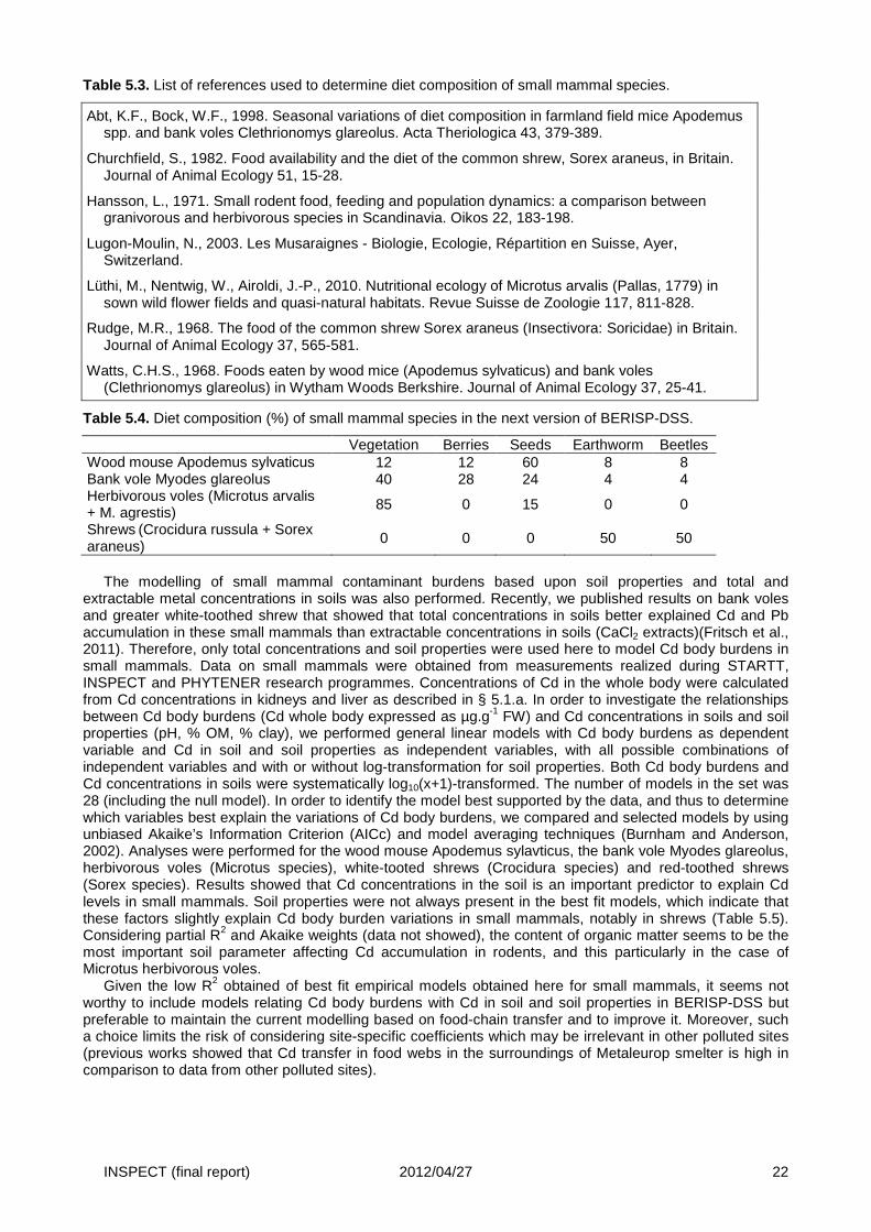
Table 5.2. Summary of analyses on Cd concentrations in stomach contents (general linear models).
Dependent variable Independent variables
p-value model
R2 model
p-value independent
variable
Partial R 2 independent
variable Cd stomach content dry weight (µg.g) < 0.001 0.58
[Cd]soil < 0.001 0.02 Genus < 0.001 0.54 Interaction [Cd]soil:genus < 0.001 0.02
Cd stomach content fresh weight (µg.g) < 0.001 0.61
[Cd]soil < 0.001 0.03 Genus < 0.001 0.55 Interaction [Cd]soil:genus < 0.001 0.02
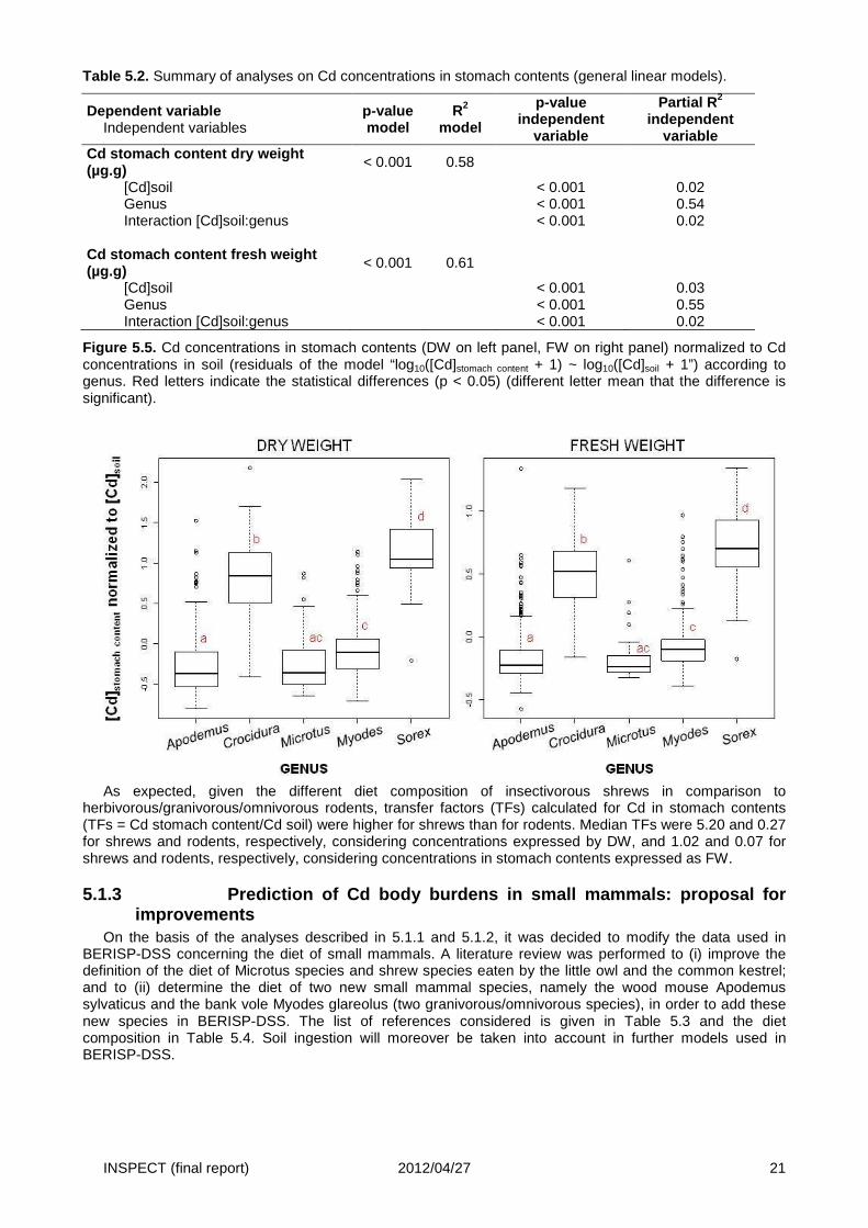
Figure 5.5. Cd concentrations in stomach contents (DW on left panel, FW on right panel) normalized to Cd concentrations in soil (residuals of the model “log10([Cd]stomach content + 1) ~ log10([Cd]soil + 1”) according to genus. Red letters indicate the statistical differences (p < 0.05) (different letter mean that the difference is significant).
As expected, given the different diet composition of insectivorous shrews in comparison to herbivorous/granivorous/omnivorous rodents, transfer factors (TFs) calculated for Cd in stomach contents (TFs = Cd stomach content/Cd soil) were higher for shrews than for rodents. Median TFs were 5.20 and 0.27 for shrews and rodents, respectively, considering concentrations expressed by DW, and 1.02 and 0.07 for shrews and rodents, respectively, considering concentrations in stomach contents expressed as FW.
5.1.3 Prediction of Cd body burdens in small mammal s: proposal for improvements
On the basis of the analyses described in 5.1.1 and 5.1.2, it was decided to modify the data used in BERISP-DSS concerning the diet of small mammals. A literature review was performed to (i) improve the definition of the diet of Microtus species and shrew species eaten by the little owl and the common kestrel; and to (ii) determine the diet of two new small mammal species, namely the wood mouse Apodemus sylvaticus and the bank vole Myodes glareolus (two granivorous/omnivorous species), in order to add these new species in BERISP-DSS. The list of references considered is given in Table 5.3 and the diet composition in Table 5.4. Soil ingestion will moreover be taken into account in further models used in BERISP-DSS.
INSPECT (final report) 2012/04/27 22
Table 5.3. List of references used to determine diet composition of small mammal species.
Abt, K.F., Bock, W.F., 1998. Seasonal variations of diet composition in farmland field mice Apodemus spp. and bank voles Clethrionomys glareolus. Acta Theriologica 43, 379-389.
Churchfield, S., 1982. Food availability and the diet of the common shrew, Sorex araneus, in Britain. Journal of Animal Ecology 51, 15-28.
Hansson, L., 1971. Small rodent food, feeding and population dynamics: a comparison between granivorous and herbivorous species in Scandinavia. Oikos 22, 183-198.
Lugon-Moulin, N., 2003. Les Musaraignes - Biologie, Ecologie, Répartition en Suisse, Ayer, Switzerland.
Lüthi, M., Nentwig, W., Airoldi, J.-P., 2010. Nutritional ecology of Microtus arvalis (Pallas, 1779) in sown wild flower fields and quasi-natural habitats. Revue Suisse de Zoologie 117, 811-828.
Rudge, M.R., 1968. The food of the common shrew Sorex araneus (Insectivora: Soricidae) in Britain. Journal of Animal Ecology 37, 565-581.
Watts, C.H.S., 1968. Foods eaten by wood mice (Apodemus sylvaticus) and bank voles (Clethrionomys glareolus) in Wytham Woods Berkshire. Journal of Animal Ecology 37, 25-41.
Table 5.4. Diet composition (%) of small mammal species in the next version of BERISP-DSS.
Vegetation Berries Seeds Earthworm Beetles Wood mouse Apodemus sylvaticus 12 12 60 8 8 Bank vole Myodes glareolus 40 28 24 4 4 Herbivorous voles (Microtus arvalis + M. agrestis) 85 0 15 0 0
Shrews (Crocidura russula + Sorex araneus) 0 0 0 50 50
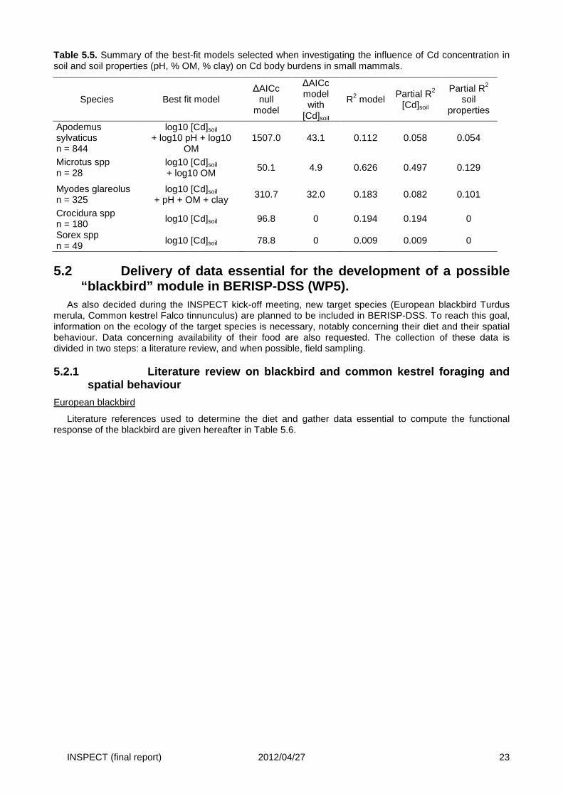
The modelling of small mammal contaminant burdens based upon soil properties and total and extractable metal concentrations in soils was also performed. Recently, we published results on bank voles and greater white-toothed shrew that showed that total concentrations in soils better explained Cd and Pb accumulation in these small mammals than extractable concentrations in soils (CaCl2 extracts)(Fritsch et al., 2011). Therefore, only total concentrations and soil properties were used here to model Cd body burdens in small mammals. Data on small mammals were obtained from measurements realized during STARTT, INSPECT and PHYTENER research programmes. Concentrations of Cd in the whole body were calculated from Cd concentrations in kidneys and liver as described in § 5.1.a. In order to investigate the relationships between Cd body burdens (Cd whole body expressed as µg.g-1 FW) and Cd concentrations in soils and soil properties (pH, % OM, % clay), we performed general linear models with Cd body burdens as dependent variable and Cd in soil and soil properties as independent variables, with all possible combinations of independent variables and with or without log-transformation for soil properties. Both Cd body burdens and Cd concentrations in soils were systematically log10(x+1)-transformed. The number of models in the set was 28 (including the null model). In order to identify the model best supported by the data, and thus to determine which variables best explain the variations of Cd body burdens, we compared and selected models by using unbiased Akaike’s Information Criterion (AICc) and model averaging techniques (Burnham and Anderson, 2002). Analyses were performed for the wood mouse Apodemus sylavticus, the bank vole Myodes glareolus, herbivorous voles (Microtus species), white-tooted shrews (Crocidura species) and red-toothed shrews (Sorex species). Results showed that Cd concentrations in the soil is an important predictor to explain Cd levels in small mammals. Soil properties were not always present in the best fit models, which indicate that these factors slightly explain Cd body burden variations in small mammals, notably in shrews (Table 5.5). Considering partial R2 and Akaike weights (data not showed), the content of organic matter seems to be the most important soil parameter affecting Cd accumulation in rodents, and this particularly in the case of Microtus herbivorous voles.
Given the low R2 obtained of best fit empirical models obtained here for small mammals, it seems not worthy to include models relating Cd body burdens with Cd in soil and soil properties in BERISP-DSS but preferable to maintain the current modelling based on food-chain transfer and to improve it. Moreover, such a choice limits the risk of considering site-specific coefficients which may be irrelevant in other polluted sites (previous works showed that Cd transfer in food webs in the surroundings of Metaleurop smelter is high in comparison to data from other polluted sites).
INSPECT (final report) 2012/04/27 23
Table 5.5. Summary of the best-fit models selected when investigating the influence of Cd concentration in soil and soil properties (pH, % OM, % clay) on Cd body burdens in small mammals.
Species Best fit model ∆AICc
null model
∆AICc model with
[Cd]soil
R2 model Partial R2
[Cd]soil
Partial R2 soil
properties
Apodemus sylvaticus n = 844
log10 [Cd]soil + log10 pH + log10
OM 1507.0 43.1 0.112 0.058 0.054
Microtus spp n = 28
log10 [Cd]soil + log10 OM
50.1 4.9 0.626 0.497 0.129
Myodes glareolus n = 325
log10 [Cd]soil + pH + OM + clay
310.7 32.0 0.183 0.082 0.101
Crocidura spp n = 180 log10 [Cd]soil 96.8 0 0.194 0.194 0
Sorex spp n = 49 log10 [Cd]soil 78.8 0 0.009 0.009 0
5.2 Delivery of data essential for the development of a possible “blackbird” module in BERISP-DSS (WP5).
As also decided during the INSPECT kick-off meeting, new target species (European blackbird Turdus merula, Common kestrel Falco tinnunculus) are planned to be included in BERISP-DSS. To reach this goal, information on the ecology of the target species is necessary, notably concerning their diet and their spatial behaviour. Data concerning availability of their food are also requested. The collection of these data is divided in two steps: a literature review, and when possible, field sampling.
5.2.1 Literature review on blackbird and common kes trel foraging and spatial behaviour
European blackbird
Literature references used to determine the diet and gather data essential to compute the functional response of the blackbird are given hereafter in Table 5.6.
INSPECT (final report) 2012/04/27 24
Table 5.6. List of references used to determine diet composition and the functional response of the European blackbird Turdus merula.
Aubineau, J., Eraud, C., Boutin, J.M., Chil, J.L., Tesson, I., Gaboriau, C., 1999. Ecologie trophique du merle noir (Turdus merula) et de la grive musicienne (Turdus philomelos) dans les bocages de l’Ouest de la France en automne – hiver, in: Thomaidis, C., Kypridemos, N. (Eds.), International Union of Game Biologists XXIVth Congress. Hunting Fed. Macedonia, Thrace, Thessaloniki, Greece, pp. 330-351.
Baurand, P.-E., 2009. Etude du régime alimentaire et de la contamination des organes de Merles noirs Turdus merula le long d'un gradient de contamination métallique. Université de Franche-Comté, UMR Chrono-Environnement, Besançon, France, p. 22.
Chamberlain, D.E., Hatchwell, B.J., Perrins, C.M., 1999. Importance of feeding ecology to the reproductive success of Blackbirds Turdus merula nesting in rural habitats. Ibis 141, 415-427.
Collinge, W.E., 1941. The food of the blackbird (Turdus merula) in successive years. Ibis 83, 610-613.
Cramp, S., 1988. Handbook of the birds of Europe, the Middle East and North Africa. Oxford University Press, Oxford, UK.
Snow, D.W., 1958. The breeding of the blackbird Turdus merula at Oxford. Ibis 100, 1-30.
Török, J., 1981. Food composition of nestling blackbirds in an oak forest bordering on an orchard. Opuscula Zoologica Budapest 17-18, 145-156.
Török, J., 1985. Comparative ecological studies on blackbird (Turdus merula) and song thrush (T. philomelos) populations. I. Nutritional ecology. Opuscula Zoologica Budapest 21, 105-135.
Török, J., Ludvig, E., 1988. Seasonal changes in foraging strategies of nesting blackbirds (Turdus merula L.). Behavioral Ecology and Sociobiology (Historical Archive) 22, 329-333.
Poole, A.E., Stillman, R.A., Watson, H.K., Norris, K.J., 2007. Searching efficiency and the functional response of a pause-travel forager. Functional Ecology 21, 784-792.
Cresswell, W., 1997. Interference competition at low competitor densities in blackbirds Turdus merula. Journal of Animal Ecology 66, 461-471.
Cresswell, W., 2001. Relative competitive ability does not change over time in blackbirds. Journal of Animal Ecology 70, 218-227.
Cresswell, W., Smith, R.D., Ruxton, G.D., 2001. Absolute foraging rate and susceptibility to interference competition in blackbirds varies with patch conditions. Journal of Animal Ecology 70, 228-236.
Blackbird diet is constituted of five main components: earthworms, invertebrates from leaf litter, fruits and berries, caterpillars, and adult insects from above ground, and food from man (seeds, household refuse…)(Table 5.7). The proportions of each item in the food composition are extremely variable (Table 5.7, Fig. 5.6).
Table 5.7. Diet composition (%) of the European blackbird Turdus merula according to the literature review.
Earthworms Beetles Gastropoda Vegetation (seeds, fruits, berries)
Median (the 23% remaining are mainly Diptera and caterpillars)
23% 33% 0% 31%
Median (100%= the 4 items reported here) 27% 37% 0% 36%
Min 4% 4% 0% 0% Max 80% 40% 2.5% 60%
The food composition principally depends on the season, the age (adults versus nestlings), the food availability, and the landscape (Cramp, 1988). The main differences in diet composition are observed between adults and nestlings, with an absence of vegetable food in nestling diet (Fig. 5.7).
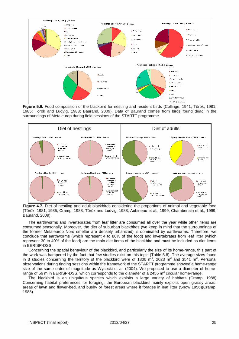
INSPECT (final report) 2012/04/27 25
Figure 5.6. Food composition of the blackbird for nestling and resident birds (Collinge, 1941; Török, 1981; 1985; Török and Ludvig, 1988; Baurand, 2009). Data of Baurand comes from birds found dead in the surroundings of Metaleurop during field sessions of the STARTT programme.
Figure 4.7. Diet of nestling and adult blackbirds considering the proportions of animal and vegetable food (Török, 1981; 1985; Cramp, 1988; Török and Ludvig, 1988; Aubineau et al., 1999; Chamberlain et al., 1999; Baurand, 2009).
The earthworms and invertebrates from leaf litter are consumed all over the year while other items are consumed seasonally. Moreover, the diet of suburban blackbirds (we keep in mind that the surroundings of the former Metaleurop Nord smelter are densely urbanized) is dominated by earthworms. Therefore, we conclude that earthworms (which represent 4 to 80% of the food) and invertebrates from leaf litter (which represent 30 to 40% of the food) are the main diet items of the blackbird and must be included as diet items in BERISP-DSS.
Concerning the spatial behaviour of the blackbird, and particularly the size of its home-range, this part of the work was hampered by the fact that few studies exist on this topic (Table 5.8). The average sizes found in 3 studies concerning the territory of the blackbird were of 1800 m2, 2023 m2 and 3541 m2. Personal observations during ringing sessions within the framework of the STARTT programme showed a home-range size of the same order of magnitude as Wysocki et al. (2004). We proposed to use a diameter of home-range of 56 m in BERISP-DSS, which corresponds to the diameter of a 2455 m2 circular home-range.
The blackbird is an ubiquitous species which exploits a large variety of habitats (Cramp, 1988) Concerning habitat preferences for foraging, the European blackbird mainly exploits open grassy areas, areas of lawn and flower-bed, and bushy or forest areas where it forages in leaf litter (Snow 1956)(Cramp, 1988).
Diet of nestlings Diet of adults
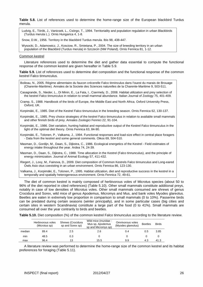
INSPECT (final report) 2012/04/27 26
Table 5.8. List of references used to determine the home-range size of the European blackbird Turdus merula.
Ludvig, E., Török, J., Vanicsek, L., Csörgo, T., 1994. Territoriality and population regulation in urban Blackbirds (Turdus merula L.). Ornis Hungarica 4, 1-8.
Snow, D.W., 1956. Territory in the blackbird Turdus merula. Ibis 98, 438-447.
Wysocki, D., Adamowicz, J., Kosciow, R., Smietana, P., 2004. The size of breeding territory in an urban population of the Blackbird (Turdus merula) in Szczecin (NW Poland). Ornis Fennica 81, 1-12.
Common kestrel
Literature references used to determine the diet and gather data essential to compute the functional response of the common kestrel are given hereafter in Table 5.9.
Table 5.9. List of references used to determine diet composition and the functional response of the common kestrel Falco tinnunculus.
Boileau, N., 2005. Régime alimentaire du faucon crécerelle Falco tinninculus dans l'ouest du marais de Brouage (Charente-Maritime). Annales de la Societe des Sciences naturelles de la Charente-Maritime 9, 503-511.
Casagrande, S., Nieder, L., Di Minin, E., La Fata, I., Csermely, D., 2008. Habitat utilization and prey selection of the kestrel Falco tinnunculus in relation to small mammal abundance. Italian Journal of Zoology 75, 401-409.
Cramp, S., 1988. Handbook of the birds of Europe, the Middle East and North Africa. Oxford University Press, Oxford, UK.
Korpimäki, E., 1985. Diet of the Kestrel Falco tinnunculus in the breeding season. Ornis Fennica 62, 130-137.
Korpimäki, E., 1985. Prey choice strategies of the kestrel Falco tinnunculus in relation to available small mammals and other finnish birds of prey. Annales Zoologici Fennici 22, 91-104.
Korpimäki, E., 1986. Diet variation, hunting habitat and reproductive output of the Kestrel Falco tinnunculus in the light of the optimal diet theory. Ornis Fennica 63, 84-90.
Korpimäki, E., Tolonen, P., Valkama, J., 1994. Functional responses and load-size effect in central place foragers - Data from the kestrel and some general comments. Oikos 69, 504-510.
Masman, D., Gordijn, M., Daan, S., Dijkstra, C., 1986. Ecological energetics of the Kestrel - Field estimates of energy intake throughout the year. Ardea 74, 24-39.
Masman, D., Daan, S., Dijkstra, C., 1988. Time allocation in the Kestrel (Falco tinnunculus), and the principle of energy minimization. Journal of Animal Ecology 57, 411-432.
Riegert, J., Lovy, M., Fainova, D., 2009. Diet composition of Common Kestrels Falco tinnunculus and Long-eared Owls Asio otus coexisting in an urban environment. Ornis Fennica 86, 123-130.
Valkama, J., Korpimäki, E., Tolonen, P., 1995. Habitat utilization, diet and reproductive success in the kestrel in a temporally and spatially heterogeneous environment. Ornis Fennica 72, 49-61.
The diet of common kestrel is mainly composed of herbivorous voles of Microtus species (about 50 to 96% of the diet reported in cited references) (Table 5.10). Other small mammals constitute additional preys, notably in case of low densities of Microtus voles. Other small mammals consumed are shrews of genus Crocidura and Sorex, wild mice of genus Apodemus, Micromys and Mus, and bank voles Myodes glareolus. Beetles are eaten in extremely low proportion in comparison to small mammals (0 to 10%). Passerine birds can be predated during certain seasons (winter principally), and in some particular cases (big cities and certain sites in western Scandinavia) constitute a large part of the food (0 to 41%). Small mammals are consumed all over the year contrarily to birds and beetles.
Table 5.10. Diet composition (%) of the common kestrel Falco tinnunculus according to the literature review.
Herbivorous voles (Microtus sp)
Shrews (Crocidura sp and Sorex sp)
Wild mice (muridae : Mus sp, Apodemus
sp and Micromys sp)
Omnivorous voles (Myodes glareolus) Beetles Birds
median 89.4 2.5 2.6 0.4 0.5 3.85
min 48.5 0.3 0 0 0 0
max 96.4 13 15.5 9.9 4.3 41.3
A literature review was performed to determine the home-range size of the common kestrel and its habitat preferences for foraging (Table 5.11).
INSPECT (final report) 2012/04/27 27
Table 5.11. List of references used to determine the home-range size of the common kestrel Falco tinnunculus.
Boileau, N., Delelis, N., Hoede, C., 2006. Use of territory and habitat selection of breeding kestrel Falco tinnunculus. Alauda 74, 251-264.
Casagrande, S., Nieder, L., Di Minin, E., La Fata, I., Csermely, D., 2008. Habitat utilization and prey selection of the kestrel Falco tinnunculus in relation to small mammal abundance. Italian Journal of Zoology 75, 401-409.
Korpimäki, E., 1986. Diet variation, hunting habitat and reproductive output of the Kestrel Falco tinnunculus in the light of the optimal diet theory. Ornis Fennica 63, 84-90.
Valkama, J., Korpimäki, E., Tolonen, P., 1995. Habitat utilization, diet and reproductive success in the kestrel in a temporally and spatially heterogeneous environment. Ornis Fennica 72, 49-61.
Village, A., 1982. Home range and density of kestrels in relation to vole abundance. Journal of Animal Ecology 51, 413-428.
The home-range size of kestrels varies notably with the availability of food and the suitability of habitats present within the area. Values from 0.74 km2 (Casagrande et al., 2008) to 13 km2 are reported (Boileau et al., 2006). However, values found in the literature are generally concordant and about 2 km2. In a recent study dealing with the modelling of the influence of environmental heterogeneity on trace metal exposure concentrations for terrestrial vertebrates, authors used a value of 2.05 km2 according to the literature review they performed (Schipper et al., 2008). We proposed to use a diameter of home-range of 1596 m in BERISP-DSS, which corresponds to the diameter of a 2 km2 circular home-range.
The common kestrel is present in a large variety of inhabited, cultivated and natural landscapes. For foraging, this raptor mainly exploits grasslands, cultivated fields, inhabited areas, marshlands, open grassy or bushy areas such as dikes, road verges, brown fields, riverbanks, abandoned fields, whereas it avoids forest areas (Korpimäki, 1986; Cramp, 1988; Boileau et al., 2006; Casagrande et al., 2008).
5.2.2 Analyses of the diet of blackbirds and common kestrels from the Metaleurop area
Analyses of the diet were performed on samples obtained over the Metaleurop area during the STARTT research programme. These analyses were performed in order (i) to check that data from the literature were concordant with the diet actually observed over the study area, and (ii) to investigate further the influence of habitat type on the diet of blackbirds (data essential for the addition of the species in BERISP-DSS because this kind of information lacks in the literature).
European blackbird
During the STARTT programme, diet items were sampled using neck collar technique on nestlings in 10 nests. Moreover, during STARTT field sessions, carcasses of blackbirds found dead over the study area were sampled, allowing the study of the diet in the stomach content of 8 birds. Diet items were identified, weighed, and classified among the four following classes: earthworm, insect (larva or adult), vegetation, and other (all other rests). To study landscape composition on the diet of blackbirds, the surface (number of pixels) of each habitat type present in a 56-m diameter buffer around dead bird location/nest location was computed. The eight habitat types were: urban and industrial facilities, arable fields, short grass (grasslands and pastures), woodland with understory (generally natural or managed forests), woodland without understory (principally tree plantations), hedgerows and copses, tall grass (tall grass, reed beds, brownfields) and shrubs, and finally watercourses and ponds. A canonical correspondence analysis was used to examine the relationships between habitat and diet.
Blackbirds mainly fed on earthworms (56 %) and insects (26 %), while vegetation and other items such as spiders, myriapods or slugs represented 4 and 14 %, respectively, of the total diet weights. Landscape composition influenced the diet composition (R2-adj = 0.125). The first and second canonical axes accounted for 25% and 18% of the total inertia, respectively, 48% and 33% of the constrained inertia, respectively, and explained 10.1% of the variance (Fig. 5.8). Globally, we obtained a gradient from diet composed mostly by earthworms versus diet composed mainly by insects or other items. Vegetation amount poorly varied among individuals and were not related to a particular habitat. Earthworms in the diet increased notably with woodland with understory and short grass, while consumption of insects and other items seemed to be dependent on the presence of woodland without understory, urban areas, hedgerows/copses and water. The influence of tall grass and shrubs is not clear, both earthworm and other items being associated with the presence of these habitats. These data were used to determine values introduced in the tables of BERISP-DSS that concern habitat-related diet preferences.
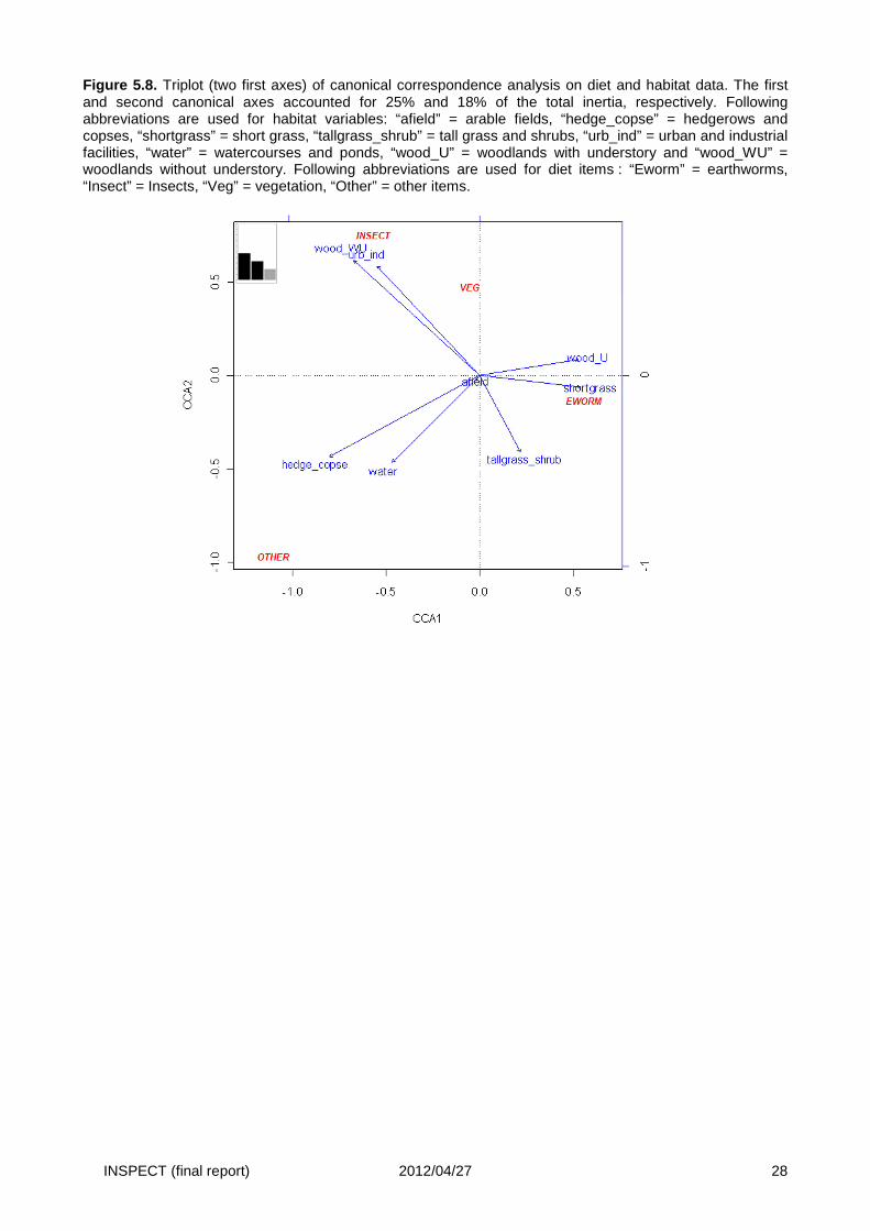
INSPECT (final report) 2012/04/27 28
Figure 5.8. Triplot (two first axes) of canonical correspondence analysis on diet and habitat data. The first and second canonical axes accounted for 25% and 18% of the total inertia, respectively. Following abbreviations are used for habitat variables: “afield” = arable fields, “hedge_copse” = hedgerows and copses, “shortgrass” = short grass, “tallgrass_shrub” = tall grass and shrubs, “urb_ind” = urban and industrial facilities, “water” = watercourses and ponds, “wood_U” = woodlands with understory and “wood_WU” = woodlands without understory. Following abbreviations are used for diet items : “Eworm” = earthworms, “Insect” = Insects, “Veg” = vegetation, “Other” = other items.
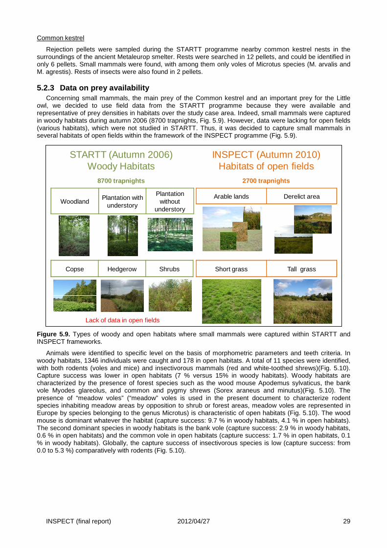
INSPECT (final report) 2012/04/27 29
Common kestrel
Rejection pellets were sampled during the STARTT programme nearby common kestrel nests in the surroundings of the ancient Metaleurop smelter. Rests were searched in 12 pellets, and could be identified in only 6 pellets. Small mammals were found, with among them only voles of Microtus species (M. arvalis and M. agrestis). Rests of insects were also found in 2 pellets.
5.2.3 Data on prey availability Concerning small mammals, the main prey of the Common kestrel and an important prey for the Little
owl, we decided to use field data from the STARTT programme because they were available and representative of prey densities in habitats over the study case area. Indeed, small mammals were captured in woody habitats during autumn 2006 (8700 trapnights, Fig. 5.9). However, data were lacking for open fields (various habitats), which were not studied in STARTT. Thus, it was decided to capture small mammals in several habitats of open fields within the framework of the INSPECT programme (Fig. 5.9).
Figure 5.9. Types of woody and open habitats where small mammals were captured within STARTT and INSPECT frameworks.
Animals were identified to specific level on the basis of morphometric parameters and teeth criteria. In woody habitats, 1346 individuals were caught and 178 in open habitats. A total of 11 species were identified, with both rodents (voles and mice) and insectivorous mammals (red and white-toothed shrews)(Fig. 5.10). Capture success was lower in open habitats (7 % versus 15% in woody habitats). Woody habitats are characterized by the presence of forest species such as the wood mouse Apodemus sylvaticus, the bank vole Myodes glareolus, and common and pygmy shrews (Sorex araneus and minutus)(Fig. 5.10). The presence of “meadow voles” (“meadow” voles is used in the present document to characterize rodent species inhabiting meadow areas by opposition to shrub or forest areas, meadow voles are represented in Europe by species belonging to the genus Microtus) is characteristic of open habitats (Fig. 5.10). The wood mouse is dominant whatever the habitat (capture success: 9.7 % in woody habitats, 4.1 % in open habitats). The second dominant species in woody habitats is the bank vole (capture success: 2.9 % in woody habitats, 0.6 % in open habitats) and the common vole in open habitats (capture success: 1.7 % in open habitats, 0.1 % in woody habitats). Globally, the capture success of insectivorous species is low (capture success: from 0.0 to 5.3 %) comparatively with rodents (Fig. 5.10).
Short grass Tall grass
STARTT (Autumn 2006)Woody Habitats
8700 trapnights
Copse Hedgerow Shrubs
WoodlandPlantation with
understory
Plantation without
understory
Arable lands Derelict area
INSPECT (Autumn 2010)Habitats of open fields
2700 trapnights
Lack of data in open fields
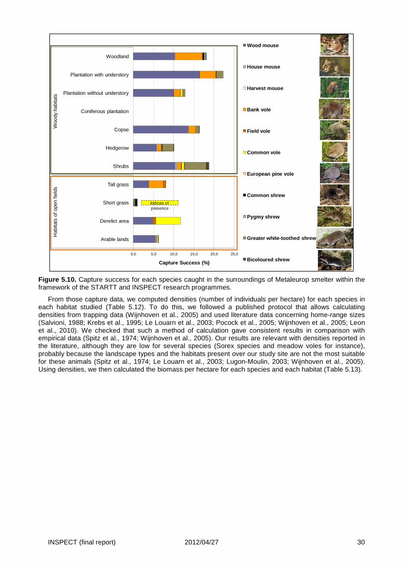
INSPECT (final report) 2012/04/27 30
Figure 5.10. Capture success for each species caught in the surroundings of Metaleurop smelter within the framework of the STARTT and INSPECT research programmes.
From those capture data, we computed densities (number of individuals per hectare) for each species in each habitat studied (Table 5.12). To do this, we followed a published protocol that allows calculating densities from trapping data (Wijnhoven et al., 2005) and used literature data concerning home-range sizes (Salvioni, 1988; Krebs et al., 1995; Le Louarn et al., 2003; Pocock et al., 2005; Wijnhoven et al., 2005; Leon et al., 2010). We checked that such a method of calculation gave consistent results in comparison with empirical data (Spitz et al., 1974; Wijnhoven et al., 2005). Our results are relevant with densities reported in the literature, although they are low for several species (Sorex species and meadow voles for instance), probably because the landscape types and the habitats present over our study site are not the most suitable for these animals (Spitz et al., 1974; Le Louarn et al., 2003; Lugon-Moulin, 2003; Wijnhoven et al., 2005). Using densities, we then calculated the biomass per hectare for each species and each habitat (Table 5.13).
Indices of presence
0,0 5,0 10,0 15,0 20,0 25,0
Arable lands
Derelict area
Short grass
Tall grass
Shrubs
Hedgerow
Copse
Coniferous plantation
Plantation without understory
Plantation with understory
WoodlandH
abita
ts o
f ope
n fie
lds
Woo
dy h
abita
ts
Capture Success (%)
Wood mouse
House mouse
Harvest mouse
Bank vole
Field vole
Common vole
European pine vole
Common shrew
Pygmy shrew
Greater white-toothed shrew
Bicoloured shrew
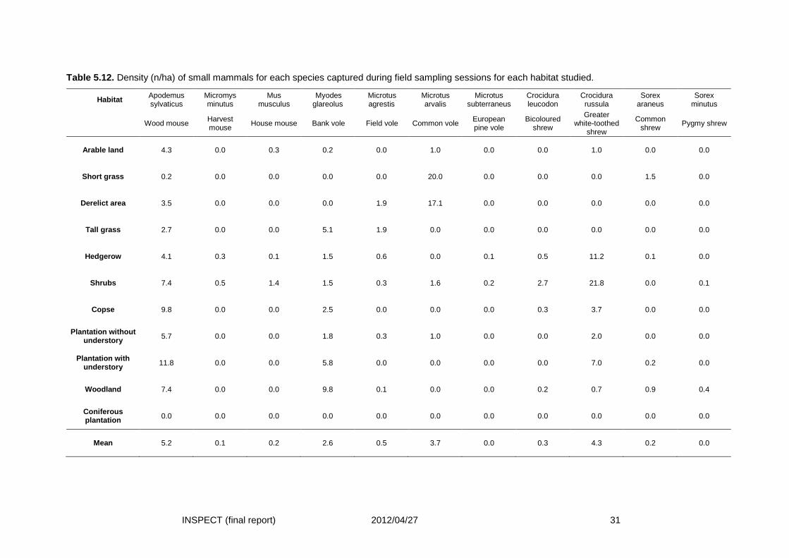
INSPECT (final report) 2012/04/27 31
Table 5.12. Density (n/ha) of small mammals for each species captured during field sampling sessions for each habitat studied.
Habitat Apodemus sylvaticus
Micromys minutus
Mus musculus
Myodes glareolus
Microtus agrestis
Microtus arvalis
Microtus subterraneus
Crocidura leucodon
Crocidura russula
Sorex araneus
Sorex minutus
Wood mouse Harvest mouse
House mouse Bank vole Field vole Common vole European pine vole
Bicoloured shrew
Greater white-toothed
shrew
Common shrew
Pygmy shrew
Arable land 4.3 0.0 0.3 0.2 0.0 1.0 0.0 0.0 1.0 0.0 0.0
Short grass 0.2 0.0 0.0 0.0 0.0 20.0 0.0 0.0 0.0 1.5 0.0
Derelict area 3.5 0.0 0.0 0.0 1.9 17.1 0.0 0.0 0.0 0.0 0.0
Tall grass 2.7 0.0 0.0 5.1 1.9 0.0 0.0 0.0 0.0 0.0 0.0
Hedgerow 4.1 0.3 0.1 1.5 0.6 0.0 0.1 0.5 11.2 0.1 0.0
Shrubs 7.4 0.5 1.4 1.5 0.3 1.6 0.2 2.7 21.8 0.0 0.1
Copse 9.8 0.0 0.0 2.5 0.0 0.0 0.0 0.3 3.7 0.0 0.0
Plantation without understory 5.7 0.0 0.0 1.8 0.3 1.0 0.0 0.0 2.0 0.0 0.0
Plantation with understory 11.8 0.0 0.0 5.8 0.0 0.0 0.0 0.0 7.0 0.2 0.0
Woodland 7.4 0.0 0.0 9.8 0.1 0.0 0.0 0.2 0.7 0.9 0.4
Coniferous plantation 0.0 0.0 0.0 0.0 0.0 0.0 0.0 0.0 0.0 0.0 0.0
Mean 5.2 0.1 0.2 2.6 0.5 3.7 0.0 0.3 4.3 0.2 0.0
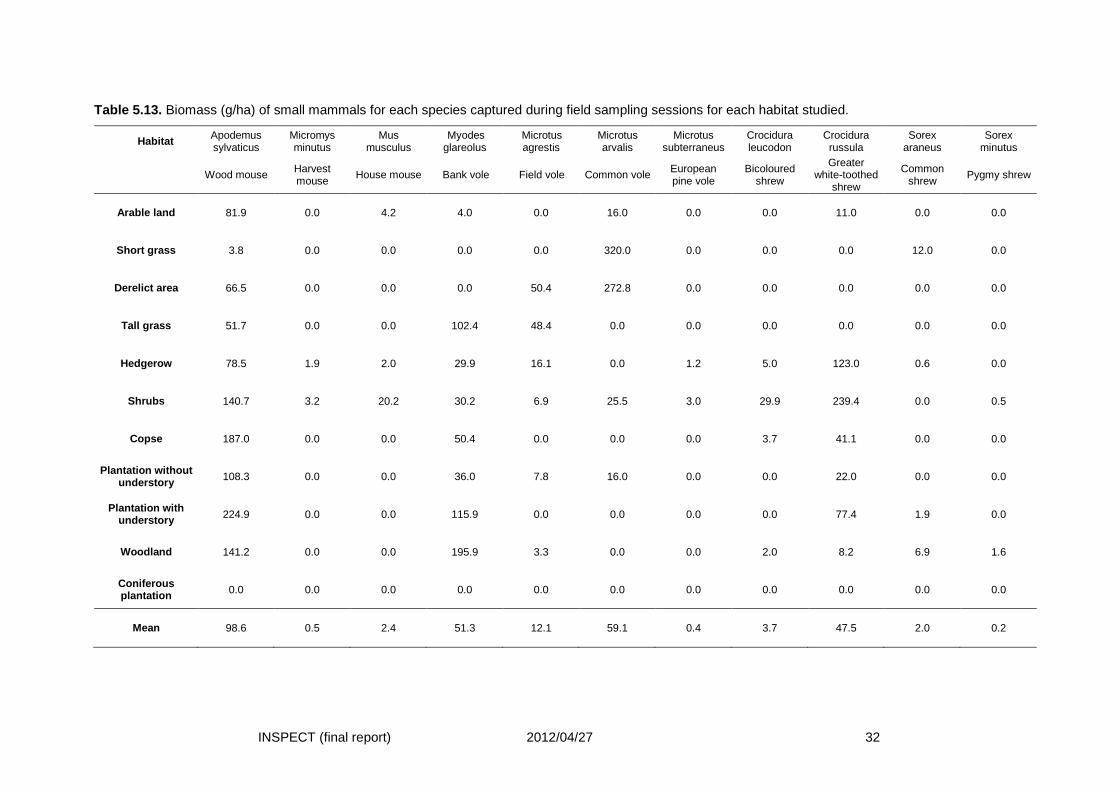
INSPECT (final report) 2012/04/27 32
Table 5.13. Biomass (g/ha) of small mammals for each species captured during field sampling sessions for each habitat studied.
Habitat Apodemus sylvaticus
Micromys minutus
Mus musculus
Myodes glareolus
Microtus agrestis
Microtus arvalis
Microtus subterraneus
Crocidura leucodon
Crocidura russula
Sorex araneus
Sorex minutus
Wood mouse Harvest mouse
House mouse Bank vole Field vole Common vole European pine vole
Bicoloured shrew
Greater white-toothed
shrew
Common shrew
Pygmy shrew
Arable land 81.9 0.0 4.2 4.0 0.0 16.0 0.0 0.0 11.0 0.0 0.0
Short grass 3.8 0.0 0.0 0.0 0.0 320.0 0.0 0.0 0.0 12.0 0.0
Derelict area 66.5 0.0 0.0 0.0 50.4 272.8 0.0 0.0 0.0 0.0 0.0
Tall grass 51.7 0.0 0.0 102.4 48.4 0.0 0.0 0.0 0.0 0.0 0.0
Hedgerow 78.5 1.9 2.0 29.9 16.1 0.0 1.2 5.0 123.0 0.6 0.0
Shrubs 140.7 3.2 20.2 30.2 6.9 25.5 3.0 29.9 239.4 0.0 0.5
Copse 187.0 0.0 0.0 50.4 0.0 0.0 0.0 3.7 41.1 0.0 0.0
Plantation without understory 108.3 0.0 0.0 36.0 7.8 16.0 0.0 0.0 22.0 0.0 0.0
Plantation with understory 224.9 0.0 0.0 115.9 0.0 0.0 0.0 0.0 77.4 1.9 0.0
Woodland 141.2 0.0 0.0 195.9 3.3 0.0 0.0 2.0 8.2 6.9 1.6
Coniferous plantation 0.0 0.0 0.0 0.0 0.0 0.0 0.0 0.0 0.0 0.0 0.0
Mean 98.6 0.5 2.4 51.3 12.1 59.1 0.4 3.7 47.5 2.0 0.2
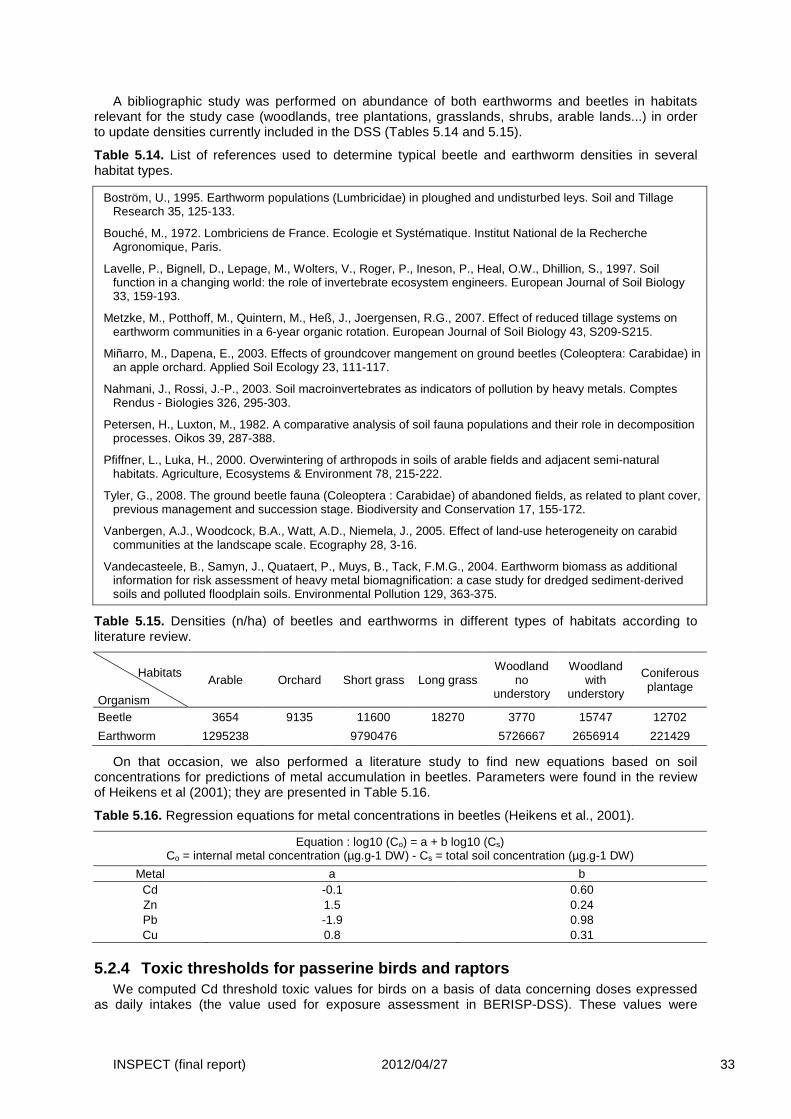
INSPECT (final report) 2012/04/27 33
A bibliographic study was performed on abundance of both earthworms and beetles in habitats relevant for the study case (woodlands, tree plantations, grasslands, shrubs, arable lands...) in order to update densities currently included in the DSS (Tables 5.14 and 5.15).
Table 5.14. List of references used to determine typical beetle and earthworm densities in several habitat types.
Boström, U., 1995. Earthworm populations (Lumbricidae) in ploughed and undisturbed leys. Soil and Tillage Research 35, 125-133.
Bouché, M., 1972. Lombriciens de France. Ecologie et Systématique. Institut National de la Recherche Agronomique, Paris.
Lavelle, P., Bignell, D., Lepage, M., Wolters, V., Roger, P., Ineson, P., Heal, O.W., Dhillion, S., 1997. Soil function in a changing world: the role of invertebrate ecosystem engineers. European Journal of Soil Biology 33, 159-193.
Metzke, M., Potthoff, M., Quintern, M., Heß, J., Joergensen, R.G., 2007. Effect of reduced tillage systems on earthworm communities in a 6-year organic rotation. European Journal of Soil Biology 43, S209-S215.
Miñarro, M., Dapena, E., 2003. Effects of groundcover mangement on ground beetles (Coleoptera: Carabidae) in an apple orchard. Applied Soil Ecology 23, 111-117.
Nahmani, J., Rossi, J.-P., 2003. Soil macroinvertebrates as indicators of pollution by heavy metals. Comptes Rendus - Biologies 326, 295-303.
Petersen, H., Luxton, M., 1982. A comparative analysis of soil fauna populations and their role in decomposition processes. Oikos 39, 287-388.
Pfiffner, L., Luka, H., 2000. Overwintering of arthropods in soils of arable fields and adjacent semi-natural habitats. Agriculture, Ecosystems & Environment 78, 215-222.
Tyler, G., 2008. The ground beetle fauna (Coleoptera : Carabidae) of abandoned fields, as related to plant cover, previous management and succession stage. Biodiversity and Conservation 17, 155-172.
Vanbergen, A.J., Woodcock, B.A., Watt, A.D., Niemela, J., 2005. Effect of land-use heterogeneity on carabid communities at the landscape scale. Ecography 28, 3-16.
Vandecasteele, B., Samyn, J., Quataert, P., Muys, B., Tack, F.M.G., 2004. Earthworm biomass as additional information for risk assessment of heavy metal biomagnification: a case study for dredged sediment-derived soils and polluted floodplain soils. Environmental Pollution 129, 363-375.
Table 5.15. Densities (n/ha) of beetles and earthworms in different types of habitats according to literature review.
Habitats Organism
Arable Orchard Short grass Long grass Woodland
no understory
Woodland with
understory
Coniferous plantage
Beetle 3654 9135 11600 18270 3770 15747 12702
Earthworm 1295238 9790476 5726667 2656914 221429
On that occasion, we also performed a literature study to find new equations based on soil concentrations for predictions of metal accumulation in beetles. Parameters were found in the review of Heikens et al (2001); they are presented in Table 5.16.
Table 5.16. Regression equations for metal concentrations in beetles (Heikens et al., 2001).
Equation : log10 (Co) = a + b log10 (Cs) Co = internal metal concentration (µg.g-1 DW) - Cs = total soil concentration (µg.g-1 DW)
Metal a b Cd -0.1 0.60 Zn 1.5 0.24 Pb -1.9 0.98 Cu 0.8 0.31
5.2.4 Toxic thresholds for passerine birds and rapt ors We computed Cd threshold toxic values for birds on a basis of data concerning doses expressed
as daily intakes (the value used for exposure assessment in BERISP-DSS). These values were
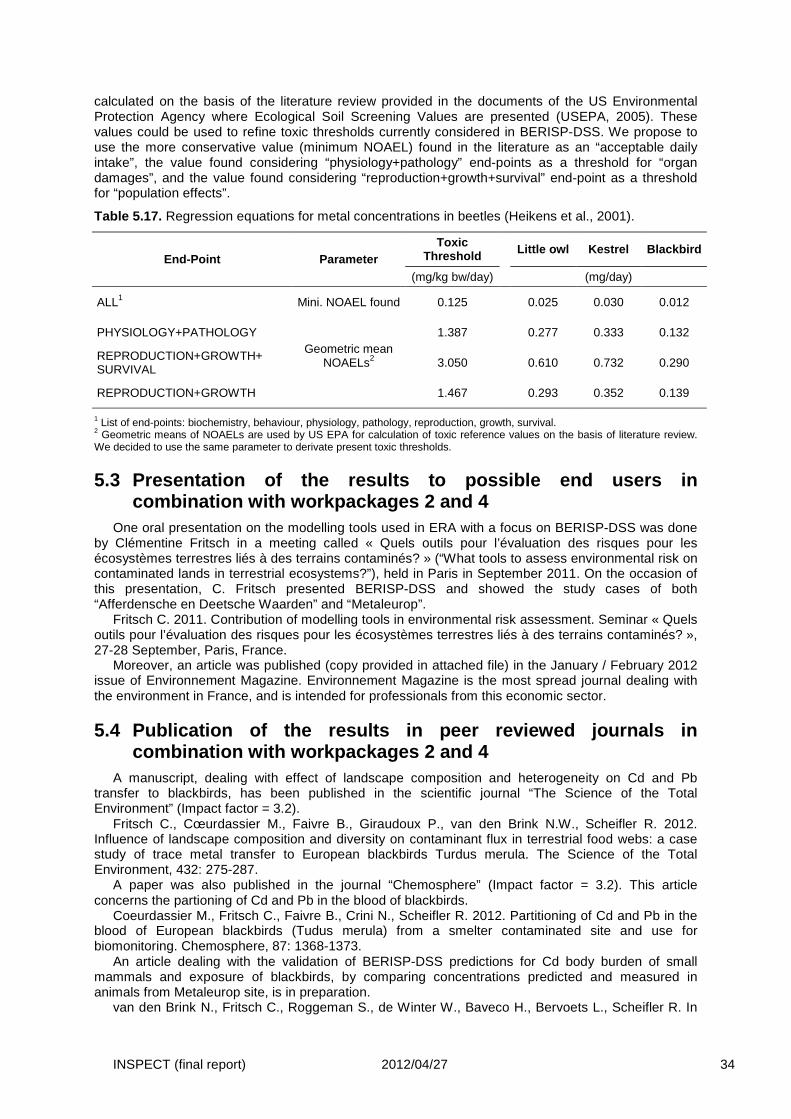
INSPECT (final report) 2012/04/27 34
calculated on the basis of the literature review provided in the documents of the US Environmental Protection Agency where Ecological Soil Screening Values are presented (USEPA, 2005). These values could be used to refine toxic thresholds currently considered in BERISP-DSS. We propose to use the more conservative value (minimum NOAEL) found in the literature as an “acceptable daily intake”, the value found considering “physiology+pathology” end-points as a threshold for “organ damages”, and the value found considering “reproduction+growth+survival” end-point as a threshold for “population effects”.
Table 5.17. Regression equations for metal concentrations in beetles (Heikens et al., 2001).
End-Point Parameter Toxic
Threshold Little owl Kestrel Blackbird
(mg/kg bw/day) (mg/day)
ALL1 Mini. NOAEL found 0.125 0.025 0.030 0.012
PHYSIOLOGY+PATHOLOGY Geometric mean
NOAELs2
1.387 0.277 0.333 0.132
REPRODUCTION+GROWTH+ SURVIVAL 3.050 0.610 0.732 0.290
REPRODUCTION+GROWTH 1.467 0.293 0.352 0.139
1 List of end-points: biochemistry, behaviour, physiology, pathology, reproduction, growth, survival. 2 Geometric means of NOAELs are used by US EPA for calculation of toxic reference values on the basis of literature review. We decided to use the same parameter to derivate present toxic thresholds.
5.3 Presentation of the results to possible end use rs in combination with workpackages 2 and 4
One oral presentation on the modelling tools used in ERA with a focus on BERISP-DSS was done by Clémentine Fritsch in a meeting called « Quels outils pour l’évaluation des risques pour les écosystèmes terrestres liés à des terrains contaminés? » (“What tools to assess environmental risk on contaminated lands in terrestrial ecosystems?”), held in Paris in September 2011. On the occasion of this presentation, C. Fritsch presented BERISP-DSS and showed the study cases of both “Afferdensche en Deetsche Waarden” and “Metaleurop”.
Fritsch C. 2011. Contribution of modelling tools in environmental risk assessment. Seminar « Quels outils pour l’évaluation des risques pour les écosystèmes terrestres liés à des terrains contaminés? », 27-28 September, Paris, France.
Moreover, an article was published (copy provided in attached file) in the January / February 2012 issue of Environnement Magazine. Environnement Magazine is the most spread journal dealing with the environment in France, and is intended for professionals from this economic sector.
5.4 Publication of the results in peer reviewed jou rnals in combination with workpackages 2 and 4
A manuscript, dealing with effect of landscape composition and heterogeneity on Cd and Pb transfer to blackbirds, has been published in the scientific journal “The Science of the Total Environment” (Impact factor = 3.2).
Fritsch C., Cœurdassier M., Faivre B., Giraudoux P., van den Brink N.W., Scheifler R. 2012. Influence of landscape composition and diversity on contaminant flux in terrestrial food webs: a case study of trace metal transfer to European blackbirds Turdus merula. The Science of the Total Environment, 432: 275-287.
A paper was also published in the journal “Chemosphere” (Impact factor = 3.2). This article concerns the partioning of Cd and Pb in the blood of blackbirds.
Coeurdassier M., Fritsch C., Faivre B., Crini N., Scheifler R. 2012. Partitioning of Cd and Pb in the blood of European blackbirds (Tudus merula) from a smelter contaminated site and use for biomonitoring. Chemosphere, 87: 1368-1373.
An article dealing with the validation of BERISP-DSS predictions for Cd body burden of small mammals and exposure of blackbirds, by comparing concentrations predicted and measured in animals from Metaleurop site, is in preparation.
van den Brink N., Fritsch C., Roggeman S., de Winter W., Baveco H., Bervoets L., Scheifler R. In
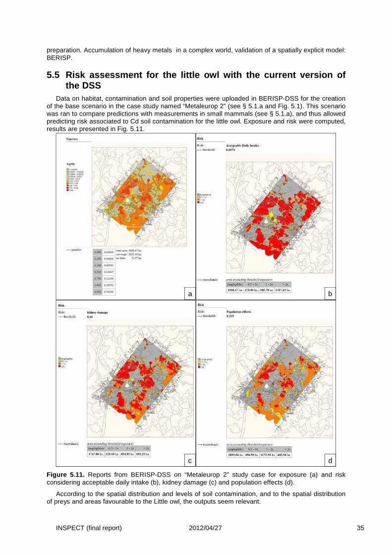
INSPECT (final report) 2012/04/27 35
preparation. Accumulation of heavy metals in a complex world, validation of a spatially explicit model: BERISP.
5.5 Risk assessment for the little owl with the cur rent version of the DSS
Data on habitat, contamination and soil properties were uploaded in BERISP-DSS for the creation of the base scenario in the case study named “Metaleurop 2” (see § 5.1.a and Fig. 5.1). This scenario was ran to compare predictions with measurements in small mammals (see § 5.1.a), and thus allowed predicting risk associated to Cd soil contamination for the little owl. Exposure and risk were computed, results are presented in Fig. 5.11.
Figure 5.11. Reports from BERISP-DSS on “Metaleurop 2” study case for exposure (a) and risk considering acceptable daily intake (b), kidney damage (c) and population effects (d).
According to the spatial distribution and levels of soil contamination, and to the spatial distribution of preys and areas favourable to the Little owl, the outputs seem relevant.
a b
c d
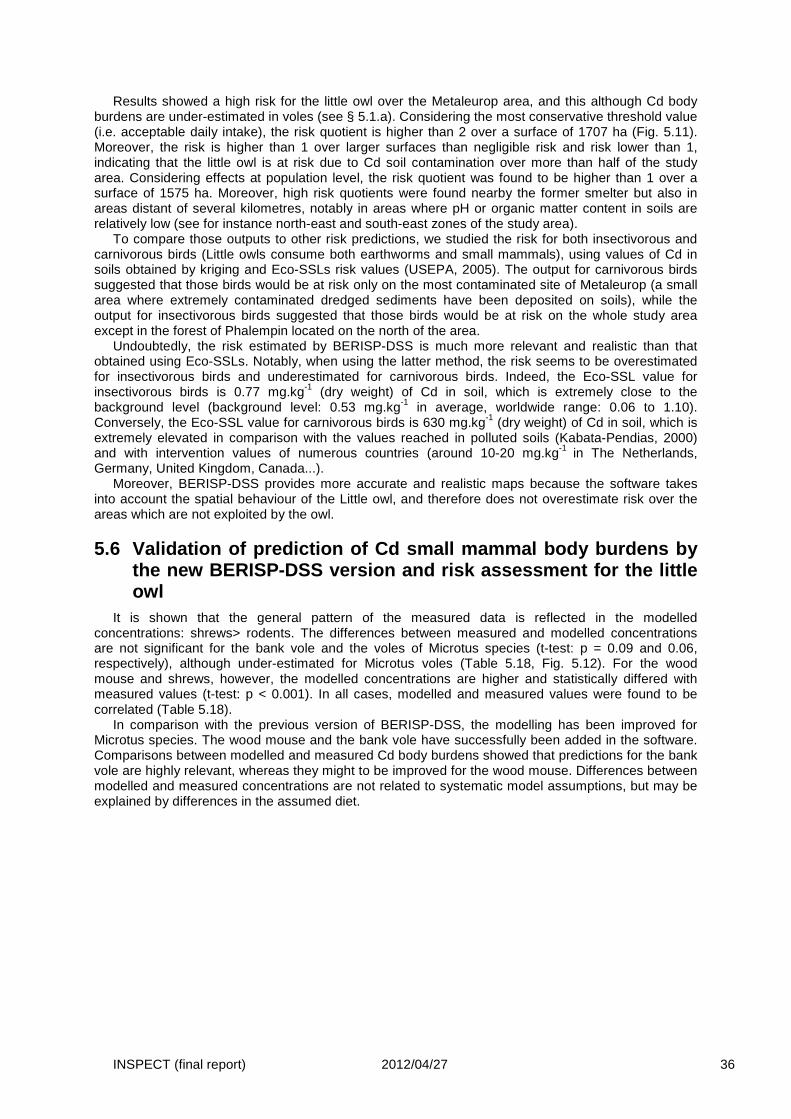
INSPECT (final report) 2012/04/27 36
Results showed a high risk for the little owl over the Metaleurop area, and this although Cd body burdens are under-estimated in voles (see § 5.1.a). Considering the most conservative threshold value (i.e. acceptable daily intake), the risk quotient is higher than 2 over a surface of 1707 ha (Fig. 5.11). Moreover, the risk is higher than 1 over larger surfaces than negligible risk and risk lower than 1, indicating that the little owl is at risk due to Cd soil contamination over more than half of the study area. Considering effects at population level, the risk quotient was found to be higher than 1 over a surface of 1575 ha. Moreover, high risk quotients were found nearby the former smelter but also in areas distant of several kilometres, notably in areas where pH or organic matter content in soils are relatively low (see for instance north-east and south-east zones of the study area).
To compare those outputs to other risk predictions, we studied the risk for both insectivorous and carnivorous birds (Little owls consume both earthworms and small mammals), using values of Cd in soils obtained by kriging and Eco-SSLs risk values (USEPA, 2005). The output for carnivorous birds suggested that those birds would be at risk only on the most contaminated site of Metaleurop (a small area where extremely contaminated dredged sediments have been deposited on soils), while the output for insectivorous birds suggested that those birds would be at risk on the whole study area except in the forest of Phalempin located on the north of the area.
Undoubtedly, the risk estimated by BERISP-DSS is much more relevant and realistic than that obtained using Eco-SSLs. Notably, when using the latter method, the risk seems to be overestimated for insectivorous birds and underestimated for carnivorous birds. Indeed, the Eco-SSL value for insectivorous birds is 0.77 mg.kg-1 (dry weight) of Cd in soil, which is extremely close to the background level (background level: 0.53 mg.kg-1 in average, worldwide range: 0.06 to 1.10). Conversely, the Eco-SSL value for carnivorous birds is 630 mg.kg-1 (dry weight) of Cd in soil, which is extremely elevated in comparison with the values reached in polluted soils (Kabata-Pendias, 2000) and with intervention values of numerous countries (around 10-20 mg.kg-1 in The Netherlands, Germany, United Kingdom, Canada...).
Moreover, BERISP-DSS provides more accurate and realistic maps because the software takes into account the spatial behaviour of the Little owl, and therefore does not overestimate risk over the areas which are not exploited by the owl.
5.6 Validation of prediction of Cd small mammal bod y burdens by the new BERISP-DSS version and risk assessment for the little owl
It is shown that the general pattern of the measured data is reflected in the modelled concentrations: shrews> rodents. The differences between measured and modelled concentrations are not significant for the bank vole and the voles of Microtus species (t-test: p = 0.09 and 0.06, respectively), although under-estimated for Microtus voles (Table 5.18, Fig. 5.12). For the wood mouse and shrews, however, the modelled concentrations are higher and statistically differed with measured values (t-test: p < 0.001). In all cases, modelled and measured values were found to be correlated (Table 5.18).
In comparison with the previous version of BERISP-DSS, the modelling has been improved for Microtus species. The wood mouse and the bank vole have successfully been added in the software. Comparisons between modelled and measured Cd body burdens showed that predictions for the bank vole are highly relevant, whereas they might to be improved for the wood mouse. Differences between modelled and measured concentrations are not related to systematic model assumptions, but may be explained by differences in the assumed diet.
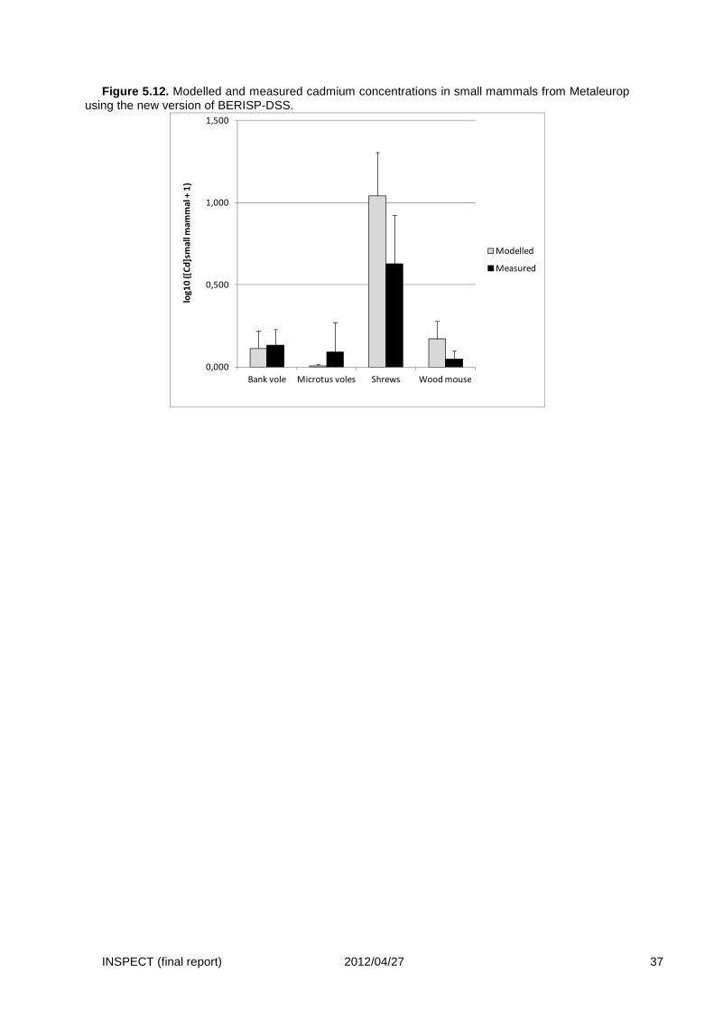
INSPECT (final report) 2012/04/27 37
Figure 5.12. Modelled and measured cadmium concentrations in small mammals from Metaleurop using the new version of BERISP-DSS.
0,000
0,500
1,000
1,500
Bank vole Microtus voles Shrews Wood mouse
log
10
([C
d]s
ma
ll m
am
ma
l + 1
)
Modelled
Measured
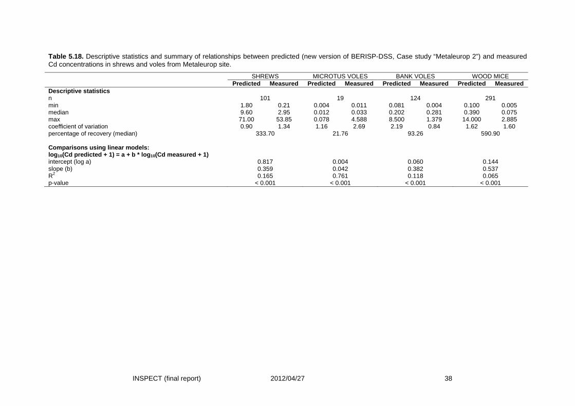
INSPECT (final report) 2012/04/27 38
Table 5.18. Descriptive statistics and summary of relationships between predicted (new version of BERISP-DSS, Case study “Metaleurop 2”) and measured Cd concentrations in shrews and voles from Metaleurop site.
SHREWS MICROTUS VOLES BANK VOLES WOOD MICE Predicted Measured Predicted Measured Predicted Measured Predicted Measured Descriptive statistics n 101 19 124 291 min 1.80 0.21 0.004 0.011 0.081 0.004 0.100 0.005 median 9.60 2.95 0.012 0.033 0.202 0.281 0.390 0.075 max 71.00 53.85 0.078 4.588 8.500 1.379 14.000 2.885 coefficient of variation 0.90 1.34 1.16 2.69 2.19 0.84 1.62 1.60 percentage of recovery (median) 333.70 21.76 93.26 590.90 Comparisons using linear models: log 10(Cd predicted + 1) = a + b * log 10(Cd measured + 1)
intercept (log a) 0.817 0.004 0.060 0.144 slope (b) 0.359 0.042 0.382 0.537 R2 0.165 0.761 0.118 0.065 p-value < 0.001 < 0.001 < 0.001 < 0.001
39
5.7 Risk assessment for the blackbird and the commo n kestrel using the new version of BERISP-DSS, and validation of prediction for the blackbird
Concentrations of Cd in some tissues of blackbirds living over Metaleurop surroundings have been measured during STARTT programme. Thus, measured data are available for comparison with exposure modelling by BERISP-DSS. Two dataset are available. The first one gathers Cd concentrations in blood and feathers from 107 birds sampled in 7 sites around the former smelter. The second one is constituted of Cd concentrations in different organs, notably liver and kidneys, from 14 birds found dead over the surroundings of the smelter during field experiment. The comparisons between modelled and measured data could not have been performed within the time allotted for INSPECT programme but will be done as soon as possible.
5.8 Synthesis on WP3
Deliverables (D)
No. of D
Title Progress
D3-1 Delivery of data essential for the validation or the optimisation of the modelling of small mammal contaminant burdens (in combination with WP5, Month 18)
Done
D3-2 Delivery of data essential for the development of a “blackbird” module in BERISP-DSS (in combination with WP5, Month 18)
Done
D3-3 Presentation of the results to possible end users (in combination with WP2 and 4, Month 12-24)
Done
D3-4 Publication of the results in peer reviewed journals (in combination with WP2 and 4, Month 12-24)
Done / in progress
40
6 Results WP4 Case Study “Campine region and Valley of the River Dommel”
The aim of WP4 is to develop a methodology for risk evaluation for grazers and spatial explicit planning of contaminated nature reserves. As a case study, a contaminated region in the North of Flanders and South of the Netherlands is chosen. The region contains nature reserves and the contaminated valley of the River Dommel (Hageven-Plateaux).
In order to be able to implement large grazers into the DSS (WP5), it is necessary to collect data and it is essential to establish scientific founded relationships between soil contamination and different types of vegetation, taking into account soil characteristics such as pH, organic content and clay content. To make the DSS generic, it is essential that those relationships are established for different types of soil and different plant species. This will ensure that end-users can assess risks of contaminated soils towards grazers in a wide variety of soil types and vegetation types.
Existing data on the metal levels in soil and vegetation from the Hageven are collected and brought together with data from literature. However, since it is very important to construct a dataset on the relationships between metals in soil and vegetation that can be applied for different soil characteristics, we collected additional samples from different contaminated soils in Flanders. Besides metals, from all soils, pH, particle size distribution and organic content will be measured (D4.1).
The grazing behaviour of the cattle within the selected area was assessed in two different seasons by following the different herds. At each site were the herds grazed vegetation samples were taken for metal analysis. Form an earlier study (BERISP project), from each individual cow, data are available on metal level in blood and hair. Both data sets will be combined.
This approach makes it possible to refine the DSS by relating the soil and vegetation contamination of the effectively visited areas by the herds to the metal levels in blood and hair of the individual cows.
Within the former projects and continued in the present project, we collected tissue samples. Literature data is currently collected on the grazing behaviour of sheep and horses in order to
construct different scenarios in the same area for other species that are not present at the moment.
6.1 Delivery of data essential for the optimization of the grazer module in the DSS
6.1.1 Introduction In order to be able to implement large grazers into the DSS (WP5), it is necessary to collect data
and it is essential to establish scientific founded relationships between soil contamination and different types of vegetation, taking into account soil characteristics such as pH, organic content and clay content. To make the DSS generic, it is essential that those relationships are established for different types of soil and different plant species. This will ensure that end-users can assess risks of contaminated soils towards grazers in a wide variety of soil types and vegetation types. Data on the transfer of metals from soil to vegetation, taking into account soil characteristics existed for the Hageven (BERISP project). However, those data did not differentiate between different plant species (or even types of vegetation). Moreover, only one type of soil (sandy soil in the Hageven-Plateaux) was considered. Therefore it was necessary to collect data on different types of (contaminated) soils and making the difference between grasses and herbs.
In a first phase, we searched in literature to find studies on the relationships between metals in soils and in vegetation that take into account the soil characteristics. Although many studies measure metals in grasses or herbs and soils, very few studies effectively investigate the relationship taking into account the soil characteristics. Moreover, in most studies accumulation modeling in food webs are based on total metal concentrations and not so much on the bioavailable or exchangeable fraction.
Therefore, in a second phase, we sampled soil, grasses and nettles at different sites in Flanders to establish these relationships and to provide multiple linear models that take into account soil characteristics. Besides measuring total metal levels in the soil we also measured exchangeable metal fractions.These models can be used to optimize the grazers module in the BERISP-DSS.
6.1.2 Materials and Methods From the mid 1950ties-70ties, zinc and lead were refined in the northern regions of Flanders.
During extraction, volatile metals were condensed on dust particles and were subsequently expelled
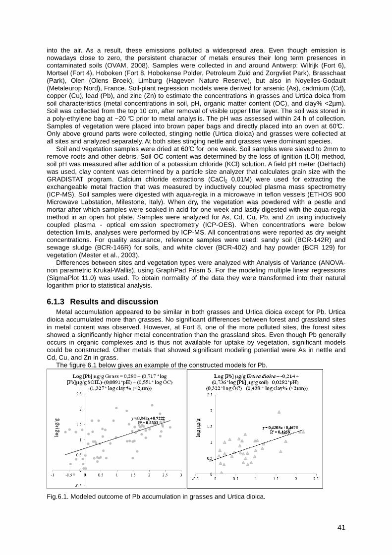
41
into the air. As a result, these emissions polluted a widespread area. Even though emission is nowadays close to zero, the persistent character of metals ensures their long term presences in contaminated soils (OVAM, 2008). Samples were collected in and around Antwerp: Wilrijk (Fort 6), Mortsel (Fort 4), Hoboken (Fort 8, Hobokense Polder, Petroleum Zuid and Zorgvliet Park), Brasschaat (Park), Olen (Olens Broek), Limburg (Hageven Nature Reserve), but also in Noyelles-Godault (Metaleurop Nord), France. Soil-plant regression models were derived for arsenic (As), cadmium (Cd), copper (Cu), lead (Pb), and zinc (Zn) to estimate the concentrations in grasses and Urtica doica from soil characteristics (metal concentrations in soil, pH, organic matter content (OC), and clay% <2µm). Soil was collected from the top 10 cm, after removal of visible upper litter layer. The soil was stored in a poly-ethylene bag at −20 °C prior to metal analys is. The pH was assessed within 24 h of collection. Samples of vegetation were placed into brown paper bags and directly placed into an oven at 60°C. Only above ground parts were collected, stinging nettle (Urtica dioica) and grasses were collected at all sites and analyzed separately. At both sites stinging nettle and grasses were dominant species.
Soil and vegetation samples were dried at 60°C for one week. Soil samples were sieved to 2mm to remove roots and other debris. Soil OC content was determined by the loss of ignition (LOI) method, soil pH was measured after addition of a potassium chloride (KCl) solution. A field pH meter (DeHach) was used, clay content was determined by a particle size analyzer that calculates grain size with the GRADISTAT program. Calcium chloride extractions (CaCl2 0,01M) were used for extracting the exchangeable metal fraction that was measured by inductively coupled plasma mass spectrometry (ICP-MS). Soil samples were digested with aqua-regia in a microwave in teflon vessels (ETHOS 900 Microwave Labstation, Milestone, Italy). When dry, the vegetation was powdered with a pestle and mortar after which samples were soaked in acid for one week and lastly digested with the aqua-regia method in an open hot plate. Samples were analyzed for As, Cd, Cu, Pb, and Zn using inductively coupled plasma - optical emission spectrometry (ICP-OES). When concentrations were below detection limits, analyses were performed by ICP-MS. All concentrations were reported as dry weight concentrations. For quality assurance, reference samples were used: sandy soil (BCR-142R) and sewage sludge (BCR-146R) for soils, and white clover (BCR-402) and hay powder (BCR 129) for vegetation (Mester et al., 2003).
Differences between sites and vegetation types were analyzed with Analysis of Variance (ANOVA-non parametric Krukal-Wallis), using GraphPad Prism 5. For the modeling multiple linear regressions (SigmaPlot 11.0) was used. To obtain normality of the data they were transformed into their natural logarithm prior to statistical analysis.
6.1.3 Results and discussion Metal accumulation appeared to be similar in both grasses and Urtica dioica except for Pb. Urtica
dioica accumulated more than grasses. No significant differences between forest and grassland sites in metal content was observed. However, at Fort 8, one of the more polluted sites, the forest sites showed a significantly higher metal concentration than the grassland sites. Even though Pb generally occurs in organic complexes and is thus not available for uptake by vegetation, significant models could be constructed. Other metals that showed significant modeling potential were As in nettle and Cd, Cu, and Zn in grass.
The figure 6.1 below gives an example of the constructed models for Pb.
Fig.6.1. Modeled outcome of Pb accumulation in grasses and Urtica dioica.
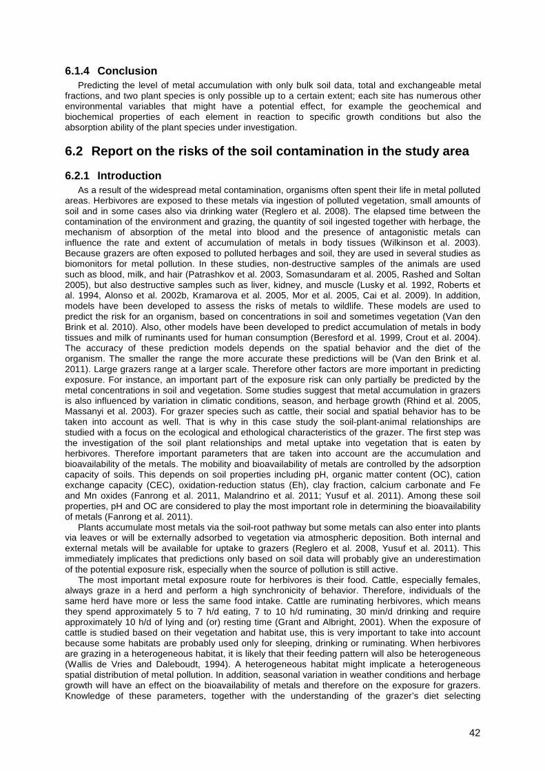
42
6.1.4 Conclusion Predicting the level of metal accumulation with only bulk soil data, total and exchangeable metal
fractions, and two plant species is only possible up to a certain extent; each site has numerous other environmental variables that might have a potential effect, for example the geochemical and biochemical properties of each element in reaction to specific growth conditions but also the absorption ability of the plant species under investigation.
6.2 Report on the risks of the soil contamination i n the study area
6.2.1 Introduction As a result of the widespread metal contamination, organisms often spent their life in metal polluted
areas. Herbivores are exposed to these metals via ingestion of polluted vegetation, small amounts of soil and in some cases also via drinking water (Reglero et al. 2008). The elapsed time between the contamination of the environment and grazing, the quantity of soil ingested together with herbage, the mechanism of absorption of the metal into blood and the presence of antagonistic metals can influence the rate and extent of accumulation of metals in body tissues (Wilkinson et al. 2003). Because grazers are often exposed to polluted herbages and soil, they are used in several studies as biomonitors for metal pollution. In these studies, non-destructive samples of the animals are used such as blood, milk, and hair (Patrashkov et al. 2003, Somasundaram et al. 2005, Rashed and Soltan 2005), but also destructive samples such as liver, kidney, and muscle (Lusky et al. 1992, Roberts et al. 1994, Alonso et al. 2002b, Kramarova et al. 2005, Mor et al. 2005, Cai et al. 2009). In addition, models have been developed to assess the risks of metals to wildlife. These models are used to predict the risk for an organism, based on concentrations in soil and sometimes vegetation (Van den Brink et al. 2010). Also, other models have been developed to predict accumulation of metals in body tissues and milk of ruminants used for human consumption (Beresford et al. 1999, Crout et al. 2004). The accuracy of these prediction models depends on the spatial behavior and the diet of the organism. The smaller the range the more accurate these predictions will be (Van den Brink et al. 2011). Large grazers range at a larger scale. Therefore other factors are more important in predicting exposure. For instance, an important part of the exposure risk can only partially be predicted by the metal concentrations in soil and vegetation. Some studies suggest that metal accumulation in grazers is also influenced by variation in climatic conditions, season, and herbage growth (Rhind et al. 2005, Massanyi et al. 2003). For grazer species such as cattle, their social and spatial behavior has to be taken into account as well. That is why in this case study the soil-plant-animal relationships are studied with a focus on the ecological and ethological characteristics of the grazer. The first step was the investigation of the soil plant relationships and metal uptake into vegetation that is eaten by herbivores. Therefore important parameters that are taken into account are the accumulation and bioavailability of the metals. The mobility and bioavailability of metals are controlled by the adsorption capacity of soils. This depends on soil properties including pH, organic matter content (OC), cation exchange capacity (CEC), oxidation-reduction status (Eh), clay fraction, calcium carbonate and Fe and Mn oxides (Fanrong et al. 2011, Malandrino et al. 2011; Yusuf et al. 2011). Among these soil properties, pH and OC are considered to play the most important role in determining the bioavailability of metals (Fanrong et al. 2011).
Plants accumulate most metals via the soil-root pathway but some metals can also enter into plants via leaves or will be externally adsorbed to vegetation via atmospheric deposition. Both internal and external metals will be available for uptake to grazers (Reglero et al. 2008, Yusuf et al. 2011). This immediately implicates that predictions only based on soil data will probably give an underestimation of the potential exposure risk, especially when the source of pollution is still active.
The most important metal exposure route for herbivores is their food. Cattle, especially females, always graze in a herd and perform a high synchronicity of behavior. Therefore, individuals of the same herd have more or less the same food intake. Cattle are ruminating herbivores, which means they spend approximately 5 to 7 h/d eating, 7 to 10 h/d ruminating, 30 min/d drinking and require approximately 10 h/d of lying and (or) resting time (Grant and Albright, 2001). When the exposure of cattle is studied based on their vegetation and habitat use, this is very important to take into account because some habitats are probably used only for sleeping, drinking or ruminating. When herbivores are grazing in a heterogeneous habitat, it is likely that their feeding pattern will also be heterogeneous (Wallis de Vries and Daleboudt, 1994). A heterogeneous habitat might implicate a heterogeneous spatial distribution of metal pollution. In addition, seasonal variation in weather conditions and herbage growth will have an effect on the bioavailability of metals and therefore on the exposure for grazers. Knowledge of these parameters, together with the understanding of the grazer’s diet selecting
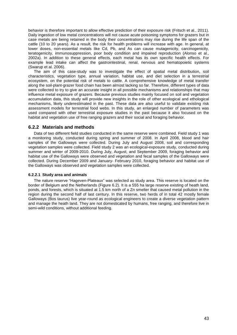
43
behavior is therefore important to allow effective prediction of their exposure risk (Fritsch et al., 2011). Daily ingestion of low metal concentrations will not cause acute poisoning symptoms for grazers but in case metals are being retained in the body their concentrations may rise during the life span of the cattle (10 to 20 years). As a result, the risk for health problems will increase with age. In general, at lower doses, non-essential metals like Cd, Pb, and As can cause mutagenicity, carcinogenicity, teratogenicity, immunosuppression, poor body condition and impaired reproduction (Alonso et al., 2002a). In addition to these general effects, each metal has its own specific health effects. For example lead intake can affect the gastrointestinal, renal, nervous and hematopoietic systems (Swarup et al. 2006).
The aim of this case-study was to investigate the effect of spatial metal distribution, soil characteristics, vegetation type, annual variation, habitat use, and diet selection in a terrestrial ecosystem, on the potential risk of metals to cattle. A comprehensive knowledge of metal transfer along the soil-plant-grazer food chain has been almost lacking so far. Therefore, different types of data were collected to try to give an accurate insight in all possible mechanisms and relationships that may influence metal exposure of grazers. Because previous studies mainly focused on soil and vegetation accumulation data, this study will provide new insights in the role of other ecological and ethological mechanisms, likely underestimated in the past. These data are also useful to validate existing risk assessment models for terrestrial food webs. In this study, an enlarged number of parameters was used compared with other terrestrial exposure studies in the past because it also focused on the habitat and vegetation use of free ranging grazers and their social and foraging behavior.
6.2.2 Materials and methods Data of two different field studies conducted in the same reserve were combined. Field study 1 was
a monitoring study, conducted during spring and summer of 2008. In April 2008, blood and hair samples of the Galloways were collected. During July and August 2008, soil and corresponding vegetation samples were collected. Field study 2 was an ecological-exposure study, conducted during summer and winter of 2009-2010. During July, August, and September 2009, foraging behavior and habitat use of the Galloways were observed and vegetation and fecal samples of the Galloways were collected. During December 2009 and January- February 2010, foraging behavior and habitat use of the Galloways was observed and vegetation samples were collected.
6.2.2.1 Study area and animals The nature reserve “Hageven-Plateaux” was selected as study area. This reserve is located on the
border of Belgium and the Netherlands (Figure 6.2). It is a 555 ha large reserve existing of heath land, ponds, and forests, which is situated at 1.5 km north of a Zn smelter that caused metal pollution in the region during the second half of last century. In this reserve, two herds of in total 42 mostly female Galloways (Bos taurus) live year-round as ecological engineers to create a diverse vegetation pattern and manage the heath land. They are not domesticated by humans, free ranging, and therefore live in semi-wild conditions, without additional feeding.
44
Fig 6.2. Map of the location of the Hageven-Plateaux reserve and the Zn smelter.
6.2.2.2 Field study 1
Soil and corresponding vegetation
During field study 1 in total 155 sampling spots were selected based on an objective grid (stratified random sampling), using ArcGis software (Figures 6.4 and 6.5). In each square of the grid, with a surface area of 40000 m2, a soil and vegetation sample was taken randomly. To locate the sampling spots in the field a ‘Garmin foretrex 201 personal navigator’ GPS was used. This allowed obtaining a non-biased insight in the spatial differences in metal pollution of the whole reserve. This grid method is often used by governments for monitoring purposes (Theocharopoulos et al. 2001).
Vegetation was collected by cutting with a stainless steel scissor from 1cm above the soil. No classification of the different vegetation types was made. One liter of soil was collected over 10 cm of depth after removal of the upper organic layer and stored in a plastic bucket using a stainless shovel. Soil samples were sieved over a 2 mm sieve, divided in 4 subsamples and stored in 50ml Falcon tubes. These subsamples were used for the analysis of metals, pH, clay fraction, and OC. The soil samples for metal analysis were dried at room temperature for 96 h. Vegetation samples were oven dried at 60° for 96h. Both soil and vegetation samp les were stored at room temperature in closed polypropylene tubes until metal analysis.
Hair and blood samples
To collect blood and hair samples during field study1, all Galloways were captured together (using hay to lure them) with the help of the nature managers from the reserve. Each blood sample was taken at the tail, by a veterinarian. Before the blood sample started clotting, 1ml blood was immediately pipetted in a preweighed 14ml Falcon tube. Back at the laboratory the 1ml samples were weighed and stored in a freezer at -20°C until anal ysis. All blood samples were freeze dried in the lab and reweighed followed by digestion for metal analysis.
Immediately after the collection of the blood sample, a hair sample was taken from the side of the neck. Hair was cut to the skin with a stainless steel scissor. The samples were put in plastic bags and stored in a freezer (-20°C) until analysis. All hai r samples were washed with acetone during 5 min. to remove external contamination. Subsequently the samples were rinsed 3 times with Milli-Q water
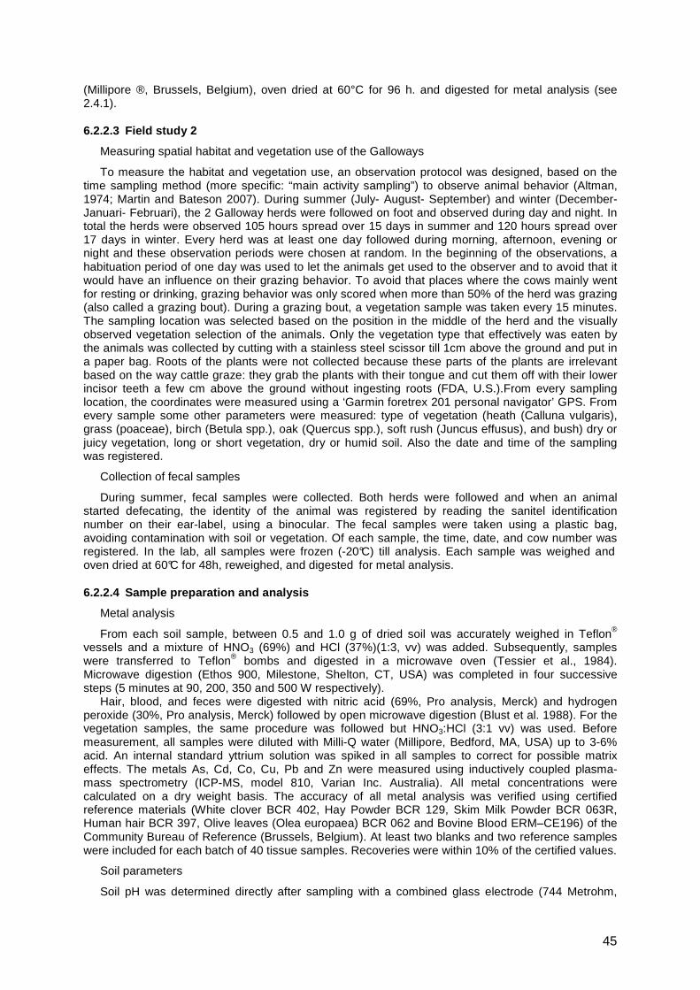
45
(Millipore ®, Brussels, Belgium), oven dried at 60°C for 96 h. and digested for metal analysis (see 2.4.1).
6.2.2.3 Field study 2
Measuring spatial habitat and vegetation use of the Galloways
To measure the habitat and vegetation use, an observation protocol was designed, based on the time sampling method (more specific: “main activity sampling”) to observe animal behavior (Altman, 1974; Martin and Bateson 2007). During summer (July- August- September) and winter (December- Januari- Februari), the 2 Galloway herds were followed on foot and observed during day and night. In total the herds were observed 105 hours spread over 15 days in summer and 120 hours spread over 17 days in winter. Every herd was at least one day followed during morning, afternoon, evening or night and these observation periods were chosen at random. In the beginning of the observations, a habituation period of one day was used to let the animals get used to the observer and to avoid that it would have an influence on their grazing behavior. To avoid that places where the cows mainly went for resting or drinking, grazing behavior was only scored when more than 50% of the herd was grazing (also called a grazing bout). During a grazing bout, a vegetation sample was taken every 15 minutes. The sampling location was selected based on the position in the middle of the herd and the visually observed vegetation selection of the animals. Only the vegetation type that effectively was eaten by the animals was collected by cutting with a stainless steel scissor till 1cm above the ground and put in a paper bag. Roots of the plants were not collected because these parts of the plants are irrelevant based on the way cattle graze: they grab the plants with their tongue and cut them off with their lower incisor teeth a few cm above the ground without ingesting roots (FDA, U.S.).From every sampling location, the coordinates were measured using a ‘Garmin foretrex 201 personal navigator’ GPS. From every sample some other parameters were measured: type of vegetation (heath (Calluna vulgaris), grass (poaceae), birch (Betula spp.), oak (Quercus spp.), soft rush (Juncus effusus), and bush) dry or juicy vegetation, long or short vegetation, dry or humid soil. Also the date and time of the sampling was registered.
Collection of fecal samples
During summer, fecal samples were collected. Both herds were followed and when an animal started defecating, the identity of the animal was registered by reading the sanitel identification number on their ear-label, using a binocular. The fecal samples were taken using a plastic bag, avoiding contamination with soil or vegetation. Of each sample, the time, date, and cow number was registered. In the lab, all samples were frozen (-20°C) till analysis. Each sample was weighed and oven dried at 60°C for 48h, reweighed, and digested for metal analysis.
6.2.2.4 Sample preparation and analysis
Metal analysis
From each soil sample, between 0.5 and 1.0 g of dried soil was accurately weighed in Teflon® vessels and a mixture of HNO3 (69%) and HCl (37%)(1:3, vv) was added. Subsequently, samples were transferred to Teflon® bombs and digested in a microwave oven (Tessier et al., 1984). Microwave digestion (Ethos 900, Milestone, Shelton, CT, USA) was completed in four successive steps (5 minutes at 90, 200, 350 and 500 W respectively).
Hair, blood, and feces were digested with nitric acid (69%, Pro analysis, Merck) and hydrogen peroxide (30%, Pro analysis, Merck) followed by open microwave digestion (Blust et al. 1988). For the vegetation samples, the same procedure was followed but HNO3:HCl (3:1 vv) was used. Before measurement, all samples were diluted with Milli-Q water (Millipore, Bedford, MA, USA) up to 3-6% acid. An internal standard yttrium solution was spiked in all samples to correct for possible matrix effects. The metals As, Cd, Co, Cu, Pb and Zn were measured using inductively coupled plasma-mass spectrometry (ICP-MS, model 810, Varian Inc. Australia). All metal concentrations were calculated on a dry weight basis. The accuracy of all metal analysis was verified using certified reference materials (White clover BCR 402, Hay Powder BCR 129, Skim Milk Powder BCR 063R, Human hair BCR 397, Olive leaves (Olea europaea) BCR 062 and Bovine Blood ERM–CE196) of the Community Bureau of Reference (Brussels, Belgium). At least two blanks and two reference samples were included for each batch of 40 tissue samples. Recoveries were within 10% of the certified values.
Soil parameters
Soil pH was determined directly after sampling with a combined glass electrode (744 Metrohm,
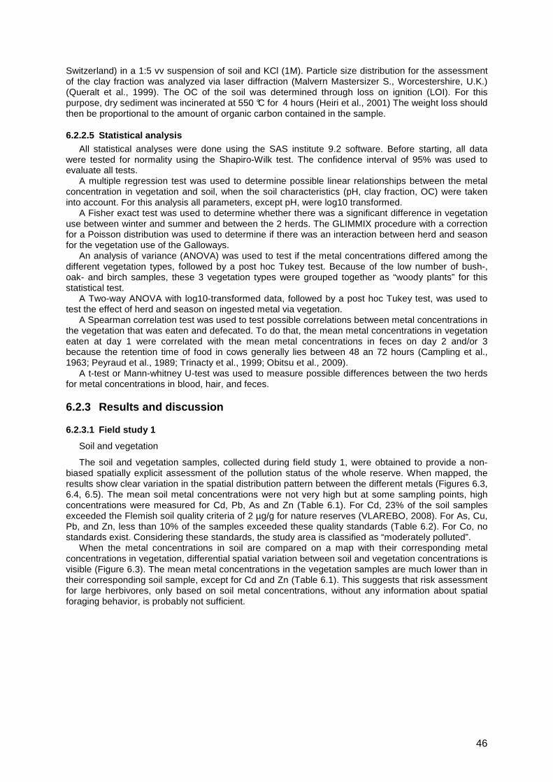
46
Switzerland) in a 1:5 vv suspension of soil and KCl (1M). Particle size distribution for the assessment of the clay fraction was analyzed via laser diffraction (Malvern Mastersizer S., Worcestershire, U.K.) (Queralt et al., 1999). The OC of the soil was determined through loss on ignition (LOI). For this purpose, dry sediment was incinerated at 550 °C for 4 hours (Heiri et al., 2001) The weight loss should then be proportional to the amount of organic carbon contained in the sample.
6.2.2.5 Statistical analysis All statistical analyses were done using the SAS institute 9.2 software. Before starting, all data
were tested for normality using the Shapiro-Wilk test. The confidence interval of 95% was used to evaluate all tests.
A multiple regression test was used to determine possible linear relationships between the metal concentration in vegetation and soil, when the soil characteristics (pH, clay fraction, OC) were taken into account. For this analysis all parameters, except pH, were log10 transformed.
A Fisher exact test was used to determine whether there was a significant difference in vegetation use between winter and summer and between the 2 herds. The GLIMMIX procedure with a correction for a Poisson distribution was used to determine if there was an interaction between herd and season for the vegetation use of the Galloways.
An analysis of variance (ANOVA) was used to test if the metal concentrations differed among the different vegetation types, followed by a post hoc Tukey test. Because of the low number of bush-, oak- and birch samples, these 3 vegetation types were grouped together as “woody plants” for this statistical test.
A Two-way ANOVA with log10-transformed data, followed by a post hoc Tukey test, was used to test the effect of herd and season on ingested metal via vegetation.
A Spearman correlation test was used to test possible correlations between metal concentrations in the vegetation that was eaten and defecated. To do that, the mean metal concentrations in vegetation eaten at day 1 were correlated with the mean metal concentrations in feces on day 2 and/or 3 because the retention time of food in cows generally lies between 48 an 72 hours (Campling et al., 1963; Peyraud et al., 1989; Trinacty et al., 1999; Obitsu et al., 2009).
A t-test or Mann-whitney U-test was used to measure possible differences between the two herds for metal concentrations in blood, hair, and feces.
6.2.3 Results and discussion
6.2.3.1 Field study 1
Soil and vegetation
The soil and vegetation samples, collected during field study 1, were obtained to provide a non-biased spatially explicit assessment of the pollution status of the whole reserve. When mapped, the results show clear variation in the spatial distribution pattern between the different metals (Figures 6.3, 6.4, 6.5). The mean soil metal concentrations were not very high but at some sampling points, high concentrations were measured for Cd, Pb, As and Zn (Table 6.1). For Cd, 23% of the soil samples exceeded the Flemish soil quality criteria of 2 µg/g for nature reserves (VLAREBO, 2008). For As, Cu, Pb, and Zn, less than 10% of the samples exceeded these quality standards (Table 6.2). For Co, no standards exist. Considering these standards, the study area is classified as “moderately polluted”.
When the metal concentrations in soil are compared on a map with their corresponding metal concentrations in vegetation, differential spatial variation between soil and vegetation concentrations is visible (Figure 6.3). The mean metal concentrations in the vegetation samples are much lower than in their corresponding soil sample, except for Cd and Zn (Table 6.1). This suggests that risk assessment for large herbivores, only based on soil metal concentrations, without any information about spatial foraging behavior, is probably not sufficient.
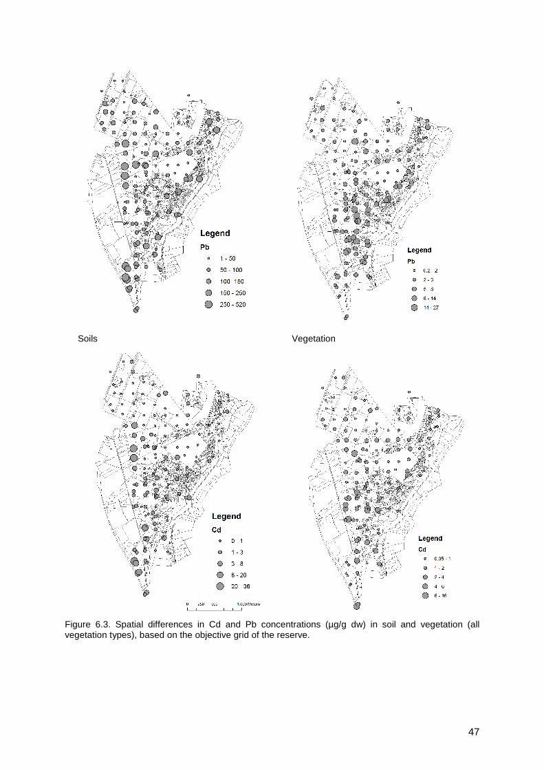
47
Soils Vegetation
Figure 6.3. Spatial differences in Cd and Pb concentrations (µg/g dw) in soil and vegetation (all vegetation types), based on the objective grid of the reserve.
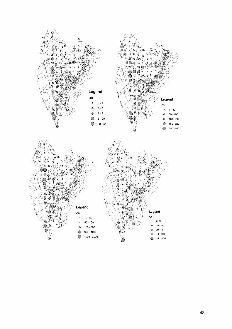
48
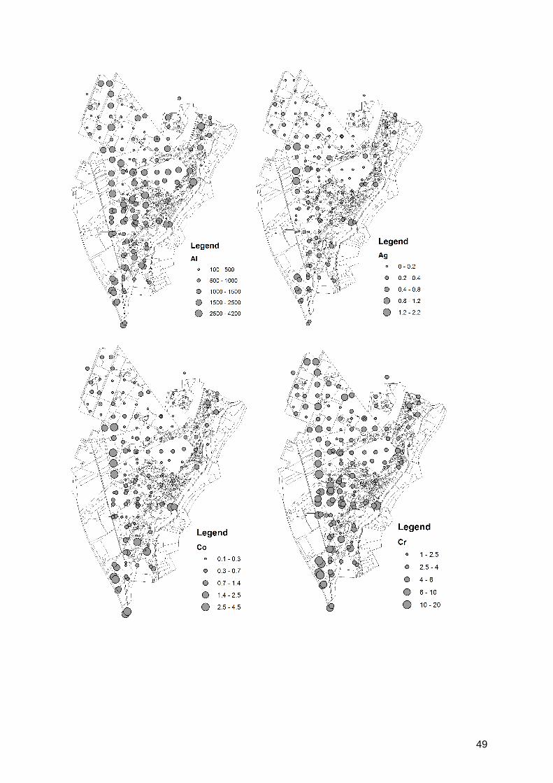
49
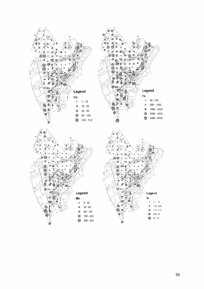
50
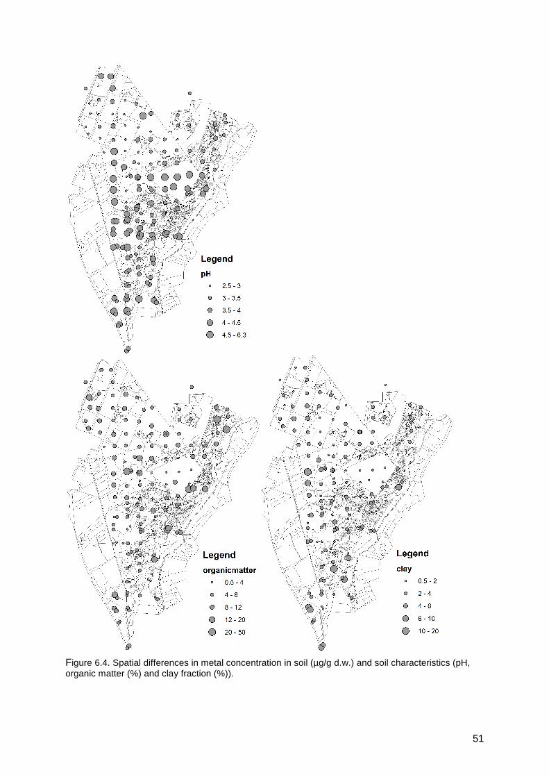
51
Figure 6.4. Spatial differences in metal concentration in soil (µg/g d.w.) and soil characteristics (pH, organic matter (%) and clay fraction (%)).
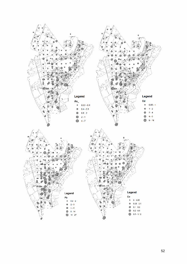
52
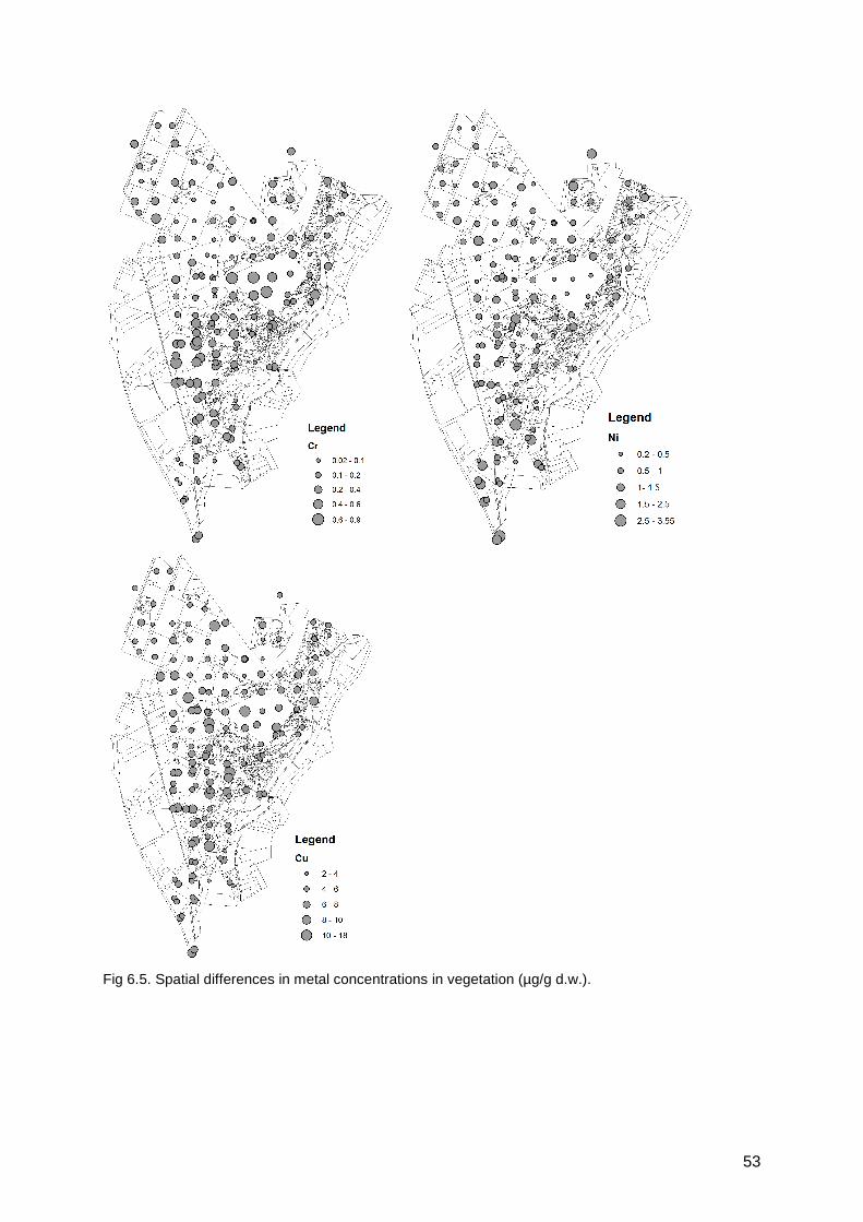
53
Fig 6.5. Spatial differences in metal concentrations in vegetation (µg/g d.w.).
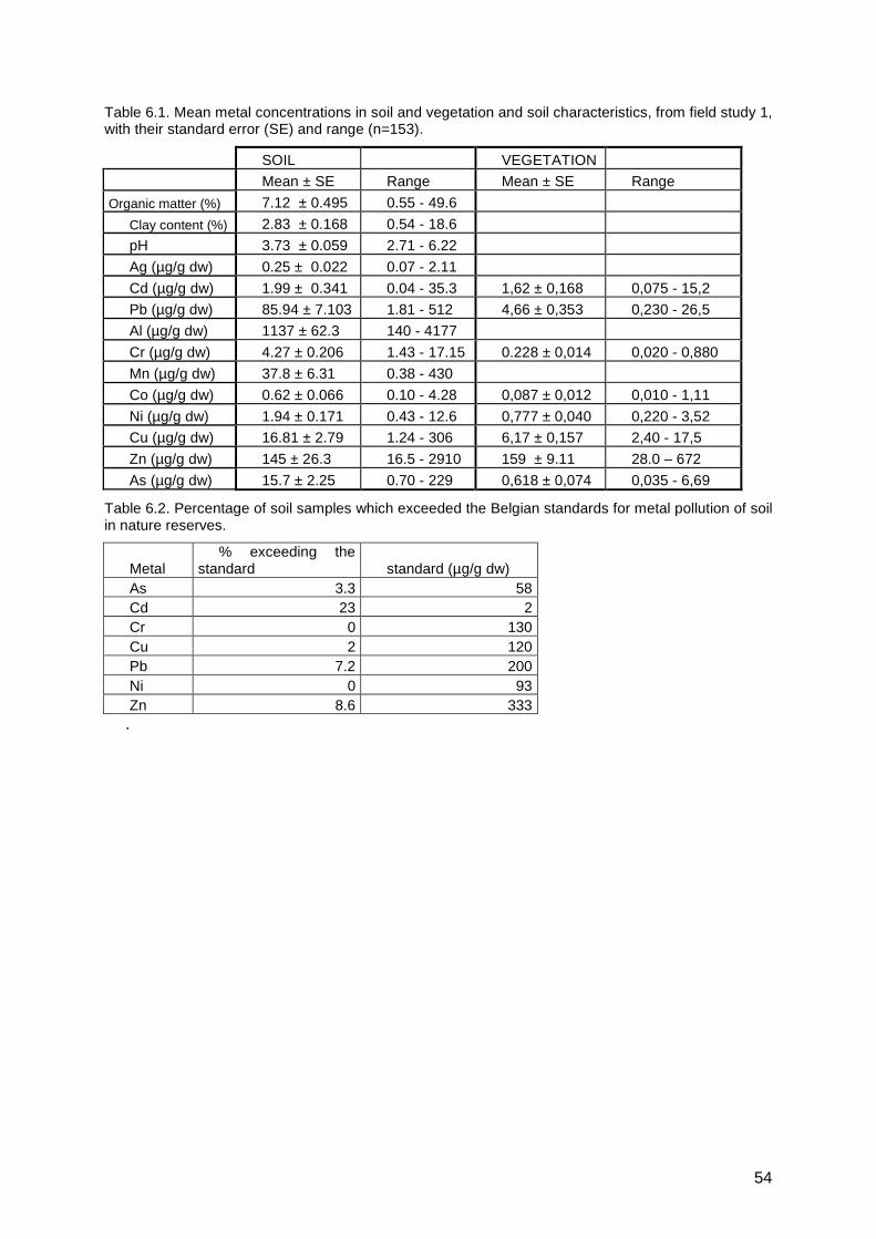
54
Table 6.1. Mean metal concentrations in soil and vegetation and soil characteristics, from field study 1, with their standard error (SE) and range (n=153).
SOIL VEGETATION
Mean ± SE Range Mean ± SE Range
Organic matter (%) 7.12 ± 0.495 0.55 - 49.6
Clay content (%) 2.83 ± 0.168 0.54 - 18.6
pH 3.73 ± 0.059 2.71 - 6.22
Ag (µg/g dw) 0.25 ± 0.022 0.07 - 2.11
Cd (µg/g dw) 1.99 ± 0.341 0.04 - 35.3 1,62 ± 0,168 0,075 - 15,2
Pb (µg/g dw) 85.94 ± 7.103 1.81 - 512 4,66 ± 0,353 0,230 - 26,5
Al (µg/g dw) 1137 ± 62.3 140 - 4177
Cr (µg/g dw) 4.27 ± 0.206 1.43 - 17.15 0.228 ± 0,014 0,020 - 0,880
Mn (µg/g dw) 37.8 ± 6.31 0.38 - 430
Co (µg/g dw) 0.62 ± 0.066 0.10 - 4.28 0,087 ± 0,012 0,010 - 1,11
Ni (µg/g dw) 1.94 ± 0.171 0.43 - 12.6 0,777 ± 0,040 0,220 - 3,52
Cu (µg/g dw) 16.81 ± 2.79 1.24 - 306 6,17 ± 0,157 2,40 - 17,5
Zn (µg/g dw) 145 ± 26.3 16.5 - 2910 159 ± 9.11 28.0 – 672
As (µg/g dw) 15.7 ± 2.25 0.70 - 229 0,618 ± 0,074 0,035 - 6,69
Table 6.2. Percentage of soil samples which exceeded the Belgian standards for metal pollution of soil in nature reserves.
Metal % exceeding the
standard standard (µg/g dw) As 3.3 58 Cd 23 2 Cr 0 130 Cu 2 120 Pb 7.2 200 Ni 0 93 Zn 8.6 333 .
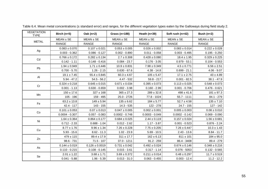
55
Table 6.4. Mean metal concentrations (± standard error) and ranges, for the different vegetation types eaten by the Galloways during field study 2.
VEGETATION TYPE
Birch ( n=5) Oak (n=2) Grass ( n=188) Heath (n=39) Soft rush ( n=42) Bush ( n=2)
METAL MEAN ± SE MEAN ± SE MEAN ± SE MEAN ± SE MEAN ± SE M EAN ± SE
RANGE RANGE RANGE RANGE RANGE RANGE
Ag 0.083 ± 0.070 0.107 ± 0.021 0.053 ± 0.005 0.026 ± 0.002 0.083 ± 0.014 0.222 ± 0.028
0.003 - 0.362 0.086 - 0.127 0.002 - 0.890 0.011 - 0.058 0.003 - 0.495 0.195 - 0.250
Cd 0.766 ± 0.172 0.282 ± 0.134 2.7 ± 0.308 0.428 ± 0.080 18.4 ± 1.95 0.329 ± 0.225
0.142 - 1.11 0.148 - 0.416 0.084 - 23.7 0.176 - 3.05 0.979 - 53.1 0.104 - 0.553
Pb 1.94 ± 0.949 1.71 ± 0.446 10.9 ± 0.831 7.98 ± 0.349 4.5 ± 0.771 6.56 ± 2.51
0.700 - 5.70 1.26 - 2.15 0.630 - 67.6 4.38 - 14.8 0.699 - 21.1 4.06 - 9.07
Al 19.1 ± 7.45 55.4 ± 0.845 60.3 ± 4.67 105 ± 5.47 17.1 ± 2.75 43 ± 4.89
5.94 - 47.2 54.5 - 56.2 4.47 - 532 59.8 - 217 0.001 - 82.5 38.1 - 47.9
Cr 0.324 ± 0.218 0.645 ± 0.015 0.671 ± 0.034 0.395 ± 0.073 0.113 ± 0.025 0.548 ± 0.073
0.001 - 1.13 0.630 - 0.659 0.002 - 3.98 0.160 - 2.99 0.001 - 0.706 0.476 - 0.621
Mn 150 ± 17.6 327 ± 168 365 ± 27.3 289 ± 32.8 498 ± 41.6 181 ± 97.3
105 - 196 159 - 495 25.0 - 2726 77.8 - 1024 55.7 - 1111 84.1 - 279
Fe 63.2 ± 13.8 149 ± 5.94 135 ± 6.62 184 ± 5.77 52.7 ± 4.58 135 ± 7.10
42.4 - 117 143 - 155 14.3 - 535 122 - 278 24.7 - 155 127 - 142
Co 0.101 ± 0.053 0.07 ± 0.013 0.047 ± 0.005 0.002 ± 0.001 0.005 ± 0.003 0.08 ± 0.010
0.0004 - 0.307 0.057 - 0.083 0.0002 - 0.748 0.0003 - 0.049 0.0002 - 0.142 0.069 - 0.090
Ni 1.64 ± 0.364 0.864 ± 0.177 0.684 ± 0.025 2.44 ± 0.119 0.157 ± 0.024 1.56 ± 0.681
0.712 - 2.33 0.688 - 1.04 0.012 - 2.62 1.17 - 3.87 0.001 - 0.523 0.876 - 2.24
Cu 8.77 ± 1.76 9.96 ± 1.34 7.26 ± 0.228 7.75 ± 0.205 7.26 ± 0.447 10.3 ± 1.43
5.93 - 15.6 8.62 - 11.3 1.02 - 23.9 5.69 - 10.5 2.43 - 13.6 8.84 - 11.7
Zn 479 ± 115 89.4 ± 17.9 311 ± 17.7 162 ± 6.13 811 ± 101 184 ± 95.0
98.6 - 731 71.5 - 107 37.0 - 1211 91.2 - 259 86.4 - 3408 89.4 - 279
As 0.144 ± 0.019 0.126 ± 0.0019 0.731 ± 0.042 0.492 ± 0.024 0.674 ± 0.146 0.348 ± 0.216
0.110 - 0.215 0.108 - 0.145 0.015 - 3.61 0.317 - 1.14 0.076 - 5053 0.132 - 0.565
Se 2.01 ± 1.22 3.68 ± 1.71 3.69 ± 0.372 0.211 ± 0.014 0.48 ± 0.297 11.7 ± 0.519
0.041 - 5.88 1.96 - 5.39 0.013 - 31.0 0.063 - 0.455 0.003 - 12.4 11.2 - 12.2
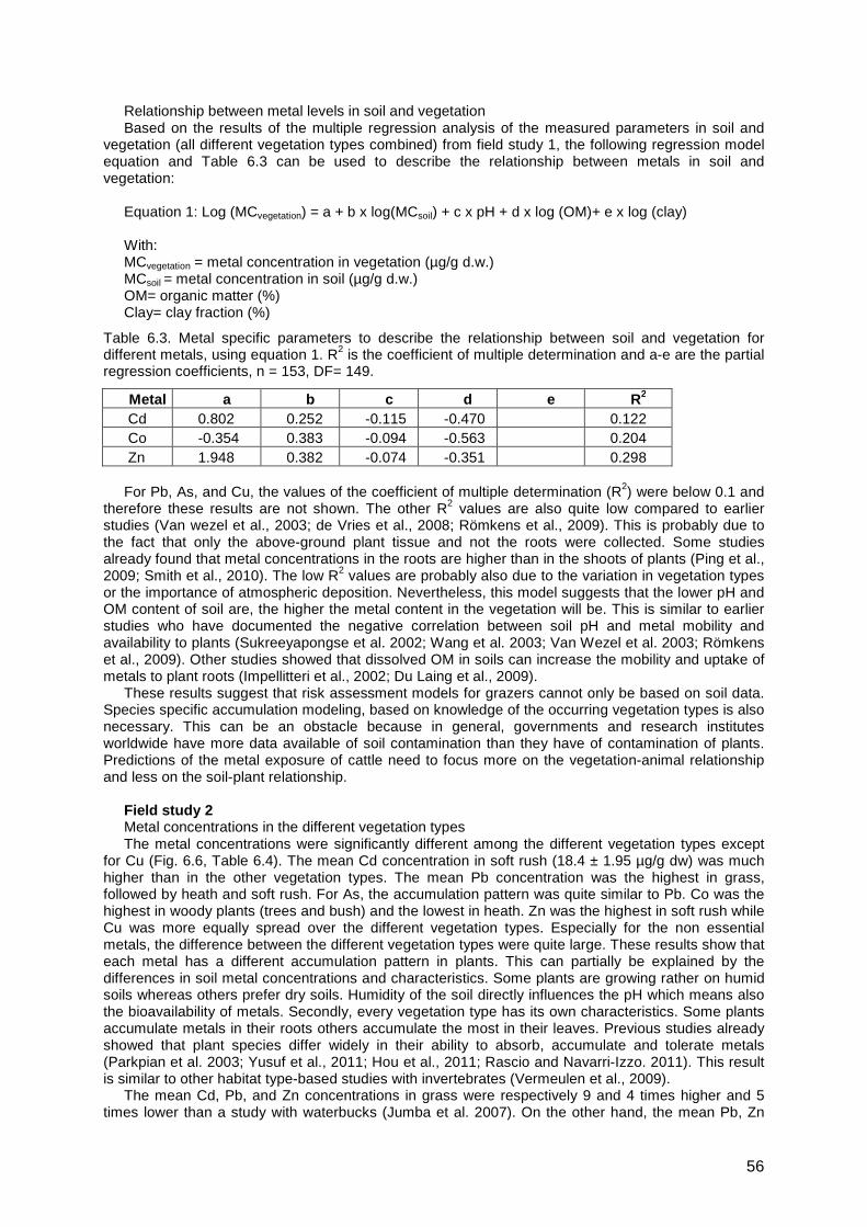
56
Relationship between metal levels in soil and vegetation Based on the results of the multiple regression analysis of the measured parameters in soil and
vegetation (all different vegetation types combined) from field study 1, the following regression model equation and Table 6.3 can be used to describe the relationship between metals in soil and vegetation:
Equation 1: Log (MCvegetation) = a + b x log(MCsoil) + c x pH + d x log (OM)+ e x log (clay)
With: MCvegetation = metal concentration in vegetation (µg/g d.w.) MCsoil = metal concentration in soil (µg/g d.w.) OM= organic matter (%) Clay= clay fraction (%)
Table 6.3. Metal specific parameters to describe the relationship between soil and vegetation for different metals, using equation 1. R2 is the coefficient of multiple determination and a-e are the partial regression coefficients, n = 153, DF= 149.
Metal a b c d e R 2
Cd 0.802 0.252 -0.115 -0.470 0.122 Co -0.354 0.383 -0.094 -0.563 0.204 Zn 1.948 0.382 -0.074 -0.351 0.298
For Pb, As, and Cu, the values of the coefficient of multiple determination (R2) were below 0.1 and
therefore these results are not shown. The other R2 values are also quite low compared to earlier studies (Van wezel et al., 2003; de Vries et al., 2008; Römkens et al., 2009). This is probably due to the fact that only the above-ground plant tissue and not the roots were collected. Some studies already found that metal concentrations in the roots are higher than in the shoots of plants (Ping et al., 2009; Smith et al., 2010). The low R2 values are probably also due to the variation in vegetation types or the importance of atmospheric deposition. Nevertheless, this model suggests that the lower pH and OM content of soil are, the higher the metal content in the vegetation will be. This is similar to earlier studies who have documented the negative correlation between soil pH and metal mobility and availability to plants (Sukreeyapongse et al. 2002; Wang et al. 2003; Van Wezel et al. 2003; Römkens et al., 2009). Other studies showed that dissolved OM in soils can increase the mobility and uptake of metals to plant roots (Impellitteri et al., 2002; Du Laing et al., 2009).
These results suggest that risk assessment models for grazers cannot only be based on soil data. Species specific accumulation modeling, based on knowledge of the occurring vegetation types is also necessary. This can be an obstacle because in general, governments and research institutes worldwide have more data available of soil contamination than they have of contamination of plants. Predictions of the metal exposure of cattle need to focus more on the vegetation-animal relationship and less on the soil-plant relationship.
Field study 2 Metal concentrations in the different vegetation types The metal concentrations were significantly different among the different vegetation types except
for Cu (Fig. 6.6, Table 6.4). The mean Cd concentration in soft rush (18.4 ± 1.95 µg/g dw) was much higher than in the other vegetation types. The mean Pb concentration was the highest in grass, followed by heath and soft rush. For As, the accumulation pattern was quite similar to Pb. Co was the highest in woody plants (trees and bush) and the lowest in heath. Zn was the highest in soft rush while Cu was more equally spread over the different vegetation types. Especially for the non essential metals, the difference between the different vegetation types were quite large. These results show that each metal has a different accumulation pattern in plants. This can partially be explained by the differences in soil metal concentrations and characteristics. Some plants are growing rather on humid soils whereas others prefer dry soils. Humidity of the soil directly influences the pH which means also the bioavailability of metals. Secondly, every vegetation type has its own characteristics. Some plants accumulate metals in their roots others accumulate the most in their leaves. Previous studies already showed that plant species differ widely in their ability to absorb, accumulate and tolerate metals (Parkpian et al. 2003; Yusuf et al., 2011; Hou et al., 2011; Rascio and Navarri-Izzo. 2011). This result is similar to other habitat type-based studies with invertebrates (Vermeulen et al., 2009).
The mean Cd, Pb, and Zn concentrations in grass were respectively 9 and 4 times higher and 5 times lower than a study with waterbucks (Jumba et al. 2007). On the other hand, the mean Pb, Zn
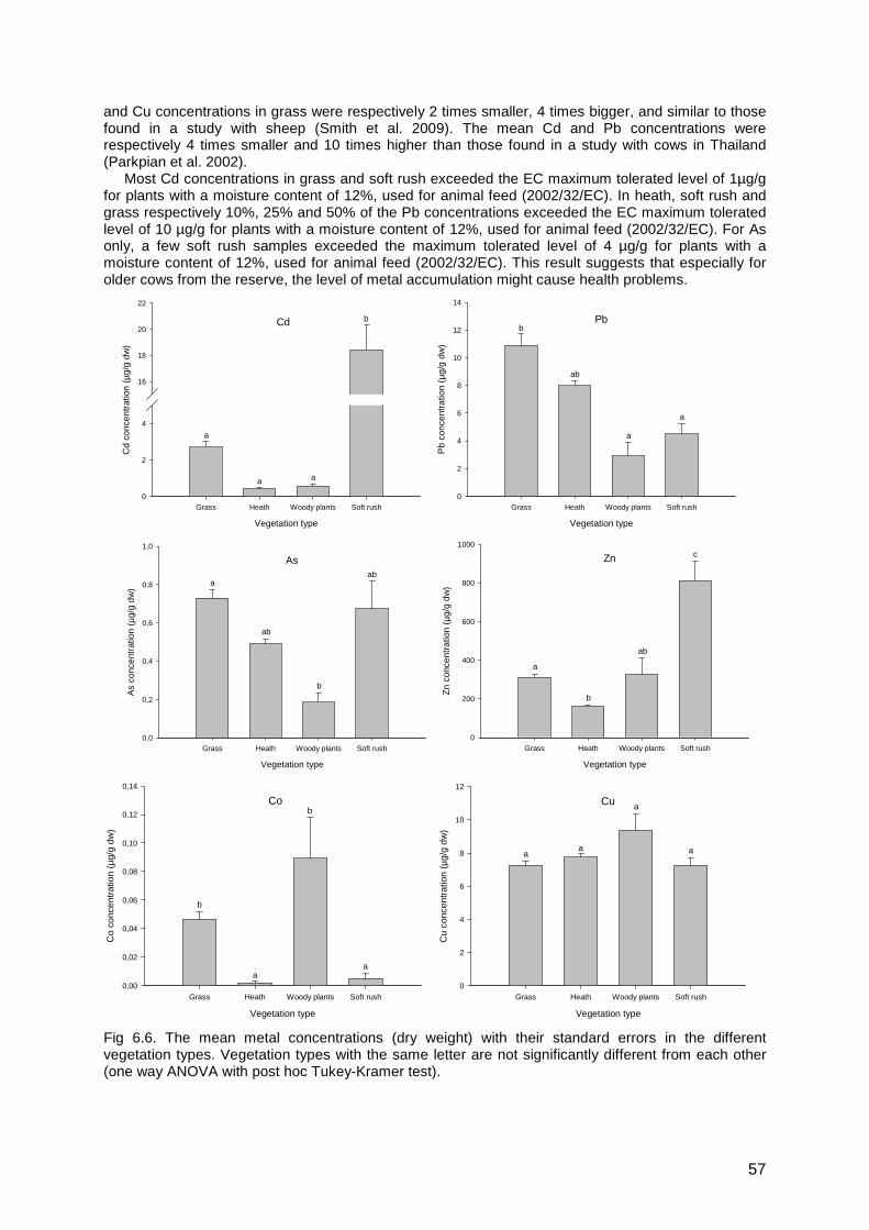
57
and Cu concentrations in grass were respectively 2 times smaller, 4 times bigger, and similar to those found in a study with sheep (Smith et al. 2009). The mean Cd and Pb concentrations were respectively 4 times smaller and 10 times higher than those found in a study with cows in Thailand (Parkpian et al. 2002).
Most Cd concentrations in grass and soft rush exceeded the EC maximum tolerated level of 1µg/g for plants with a moisture content of 12%, used for animal feed (2002/32/EC). In heath, soft rush and grass respectively 10%, 25% and 50% of the Pb concentrations exceeded the EC maximum tolerated level of 10 µg/g for plants with a moisture content of 12%, used for animal feed (2002/32/EC). For As only, a few soft rush samples exceeded the maximum tolerated level of 4 µg/g for plants with a moisture content of 12%, used for animal feed (2002/32/EC). This result suggests that especially for older cows from the reserve, the level of metal accumulation might cause health problems.
Cd
Vegetation type
Grass Heath Woody plants Soft rush
Cd
conc
entr
atio
n (µ
g/g
dw)
0
2
4
16
18
20
22
b
a
aa
Pb
Vegetation type
Grass Heath Woody plants Soft rush
Pb
conc
entr
atio
n (µ
g/g
dw)
0
2
4
6
8
10
12
14
b
a
a
ab
As
Vegetation type
Grass Heath Woody plants Soft rush
As
conc
entr
atio
n (µ
g/g
dw)
0,0
0,2
0,4
0,6
0,8
1,0
a
b
ab
ab
Zn
Vegetation type
Grass Heath Woody plants Soft rush
Zn
conc
entr
atio
n (µ
g/g
dw)
0
200
400
600
800
1000
a
b
c
ab
Co
Vegetation type
Grass Heath Woody plants Soft rush
Co
conc
entr
atio
n (µ
g/g
dw)
0,00
0,02
0,04
0,06
0,08
0,10
0,12
0,14
b
a
b
a
Cu
Vegetation type
Grass Heath Woody plants Soft rush
Cu
conc
entr
atio
n (µ
g/g
dw)
0
2
4
6
8
10
12
aa
a
a
Fig 6.6. The mean metal concentrations (dry weight) with their standard errors in the different vegetation types. Vegetation types with the same letter are not significantly different from each other (one way ANOVA with post hoc Tukey-Kramer test).
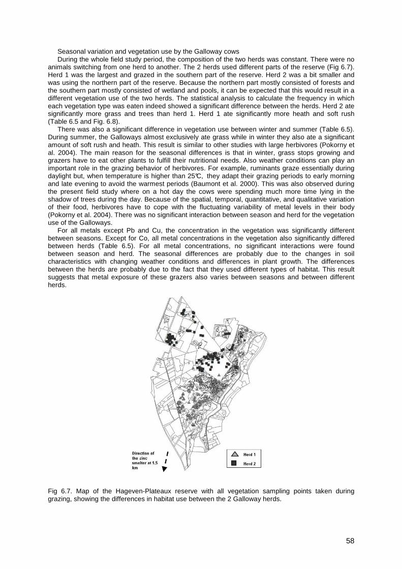
58
Seasonal variation and vegetation use by the Galloway cows During the whole field study period, the composition of the two herds was constant. There were no
animals switching from one herd to another. The 2 herds used different parts of the reserve (Fig 6.7). Herd 1 was the largest and grazed in the southern part of the reserve. Herd 2 was a bit smaller and was using the northern part of the reserve. Because the northern part mostly consisted of forests and the southern part mostly consisted of wetland and pools, it can be expected that this would result in a different vegetation use of the two herds. The statistical analysis to calculate the frequency in which each vegetation type was eaten indeed showed a significant difference between the herds. Herd 2 ate significantly more grass and trees than herd 1. Herd 1 ate significantly more heath and soft rush (Table 6.5 and Fig. 6.8).
There was also a significant difference in vegetation use between winter and summer (Table 6.5). During summer, the Galloways almost exclusively ate grass while in winter they also ate a significant amount of soft rush and heath. This result is similar to other studies with large herbivores (Pokorny et al. 2004). The main reason for the seasonal differences is that in winter, grass stops growing and grazers have to eat other plants to fulfill their nutritional needs. Also weather conditions can play an important role in the grazing behavior of herbivores. For example, ruminants graze essentially during daylight but, when temperature is higher than 25°C, they adapt their grazing periods to early morning and late evening to avoid the warmest periods (Baumont et al. 2000). This was also observed during the present field study where on a hot day the cows were spending much more time lying in the shadow of trees during the day. Because of the spatial, temporal, quantitative, and qualitative variation of their food, herbivores have to cope with the fluctuating variability of metal levels in their body (Pokorny et al. 2004). There was no significant interaction between season and herd for the vegetation use of the Galloways.
For all metals except Pb and Cu, the concentration in the vegetation was significantly different between seasons. Except for Co, all metal concentrations in the vegetation also significantly differed between herds (Table 6.5). For all metal concentrations, no significant interactions were found between season and herd. The seasonal differences are probably due to the changes in soil characteristics with changing weather conditions and differences in plant growth. The differences between the herds are probably due to the fact that they used different types of habitat. This result suggests that metal exposure of these grazers also varies between seasons and between different herds.
Fig 6.7. Map of the Hageven-Plateaux reserve with all vegetation sampling points taken during grazing, showing the differences in habitat use between the 2 Galloway herds.
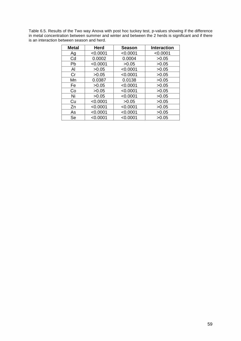
59
Table 6.5. Results of the Two way Anova with post hoc tuckey test, p-values showing if the difference in metal concentration between summer and winter and between the 2 herds is significant and if there is an interaction between season and herd.
Metal Herd Season Interaction Ag <0.0001 <0.0001 <0.0001 Cd 0.0002 0.0004 >0.05 Pb <0.0001 >0.05 >0.05 Al >0.05 <0.0001 >0.05 Cr >0.05 <0.0001 >0.05 Mn 0.0387 0.0138 >0.05 Fe >0.05 <0.0001 >0.05 Co >0.05 <0.0001 >0.05 Ni >0.05 <0.0001 >0.05 Cu <0.0001 >0.05 >0.05 Zn <0.0001 <0.0001 >0.05 As <0.0001 <0.0001 >0.05 Se <0.0001 <0.0001 >0.05
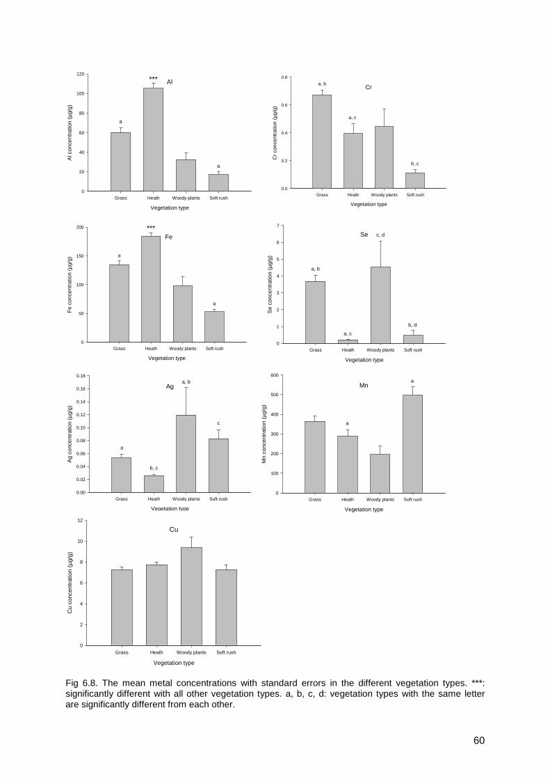
60
Fig 6.8. The mean metal concentrations with standard errors in the different vegetation types. ***: significantly different with all other vegetation types. a, b, c, d: vegetation types with the same letter are significantly different from each other.
Cr
Vegetation type
Grass Heath Woody plants Soft rush
Cr
conc
entr
atio
n (µ
g/g)
0.0
0.2
0.4
0.6
0.8
a, b
a, c
b, c
Al
Vegetation type
Grass Heath Woody plants Soft rush
Al c
once
ntra
tion
(µg/
g)
0
20
40
60
80
100
120
a
***
a
Fe
Vegetation type
Grass Heath Woody plants Soft rush
Fe
conc
entr
atio
n (µ
g/g)
0
50
100
150
200
a
a
***Se
Vegetation type
Grass Heath Woody plants Soft rush
Se
conc
entr
atio
n (µ
g/g)
0
1
2
3
4
5
6
7
a, b
a, c
c, d
b, d
Ag
Vegetation type
Grass Heath Woody plants Soft rush
Ag
conc
entr
atio
n (µ
g/g)
0.00
0.02
0.04
0.06
0.08
0.10
0.12
0.14
0.16
0.18
a
b, c
a, b
c
Mn
Vegetation type
Grass Heath Woody plants Soft rush
Mn
conc
entr
atio
n (µ
g/g)
0
100
200
300
400
500
600
a
a
Cu
Vegetation type
Grass Heath Woody plants Soft rush
Cu
conc
entr
atio
n (µ
g/g)
0
2
4
6
8
10
12
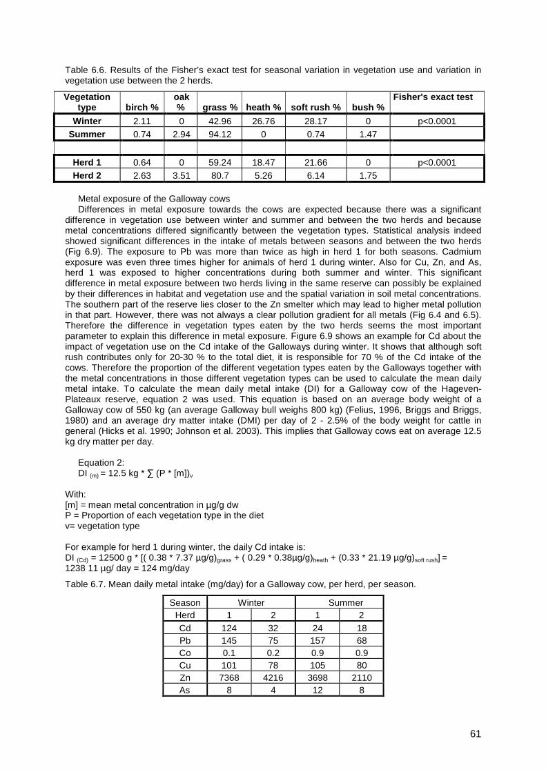
61
Table 6.6. Results of the Fisher’s exact test for seasonal variation in vegetation use and variation in vegetation use between the 2 herds.
Vegetation type birch %
oak % grass % heath % soft rush % bush %
Fisher's exact test
Winter 2.11 0 42.96 26.76 28.17 0 p<0.0001 Summer 0.74 2.94 94.12 0 0.74 1.47
Herd 1 0.64 0 59.24 18.47 21.66 0 p<0.0001 Herd 2 2.63 3.51 80.7 5.26 6.14 1.75
Metal exposure of the Galloway cows Differences in metal exposure towards the cows are expected because there was a significant
difference in vegetation use between winter and summer and between the two herds and because metal concentrations differed significantly between the vegetation types. Statistical analysis indeed showed significant differences in the intake of metals between seasons and between the two herds (Fig 6.9). The exposure to Pb was more than twice as high in herd 1 for both seasons. Cadmium exposure was even three times higher for animals of herd 1 during winter. Also for Cu, Zn, and As, herd 1 was exposed to higher concentrations during both summer and winter. This significant difference in metal exposure between two herds living in the same reserve can possibly be explained by their differences in habitat and vegetation use and the spatial variation in soil metal concentrations. The southern part of the reserve lies closer to the Zn smelter which may lead to higher metal pollution in that part. However, there was not always a clear pollution gradient for all metals (Fig 6.4 and 6.5). Therefore the difference in vegetation types eaten by the two herds seems the most important parameter to explain this difference in metal exposure. Figure 6.9 shows an example for Cd about the impact of vegetation use on the Cd intake of the Galloways during winter. It shows that although soft rush contributes only for 20-30 % to the total diet, it is responsible for 70 % of the Cd intake of the cows. Therefore the proportion of the different vegetation types eaten by the Galloways together with the metal concentrations in those different vegetation types can be used to calculate the mean daily metal intake. To calculate the mean daily metal intake (DI) for a Galloway cow of the Hageven-Plateaux reserve, equation 2 was used. This equation is based on an average body weight of a Galloway cow of 550 kg (an average Galloway bull weighs 800 kg) (Felius, 1996, Briggs and Briggs, 1980) and an average dry matter intake (DMI) per day of 2 - 2.5% of the body weight for cattle in general (Hicks et al. 1990; Johnson et al. 2003). This implies that Galloway cows eat on average 12.5 kg dry matter per day.
Equation 2: DI (m) = 12.5 kg * ∑ (P * [m])v
With: [m] = mean metal concentration in µg/g dw P = Proportion of each vegetation type in the diet v= vegetation type For example for herd 1 during winter, the daily Cd intake is: DI (Cd) = 12500 g * [( 0.38 * 7.37 µg/g)grass + ( 0.29 * 0.38µg/g)heath + (0.33 * 21.19 µg/g)soft rush] = 1238 11 µg/ day = 124 mg/day
Table 6.7. Mean daily metal intake (mg/day) for a Galloway cow, per herd, per season.
Season Winter Summer Herd 1 2 1 2 Cd 124 32 24 18 Pb 145 75 157 68 Co 0.1 0.2 0.9 0.9 Cu 101 78 105 80 Zn 7368 4216 3698 2110 As 8 4 12 8
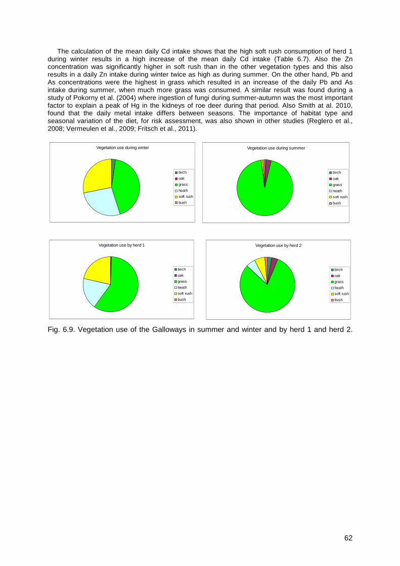
62
The calculation of the mean daily Cd intake shows that the high soft rush consumption of herd 1 during winter results in a high increase of the mean daily Cd intake (Table 6.7). Also the Zn concentration was significantly higher in soft rush than in the other vegetation types and this also results in a daily Zn intake during winter twice as high as during summer. On the other hand, Pb and As concentrations were the highest in grass which resulted in an increase of the daily Pb and As intake during summer, when much more grass was consumed. A similar result was found during a study of Pokorny et al. (2004) where ingestion of fungi during summer-autumn was the most important factor to explain a peak of Hg in the kidneys of roe deer during that period. Also Smith at al. 2010, found that the daily metal intake differs between seasons. The importance of habitat type and seasonal variation of the diet, for risk assessment, was also shown in other studies (Reglero et al., 2008; Vermeulen et al., 2009; Fritsch et al., 2011).
Fig. 6.9. Vegetation use of the Galloways in summer and winter and by herd 1 and herd 2.
Vegetation use during winter
birch
oak
grass
heath
soft rush
bush
Vegetation use during summer
birch
oak
grass
heath
soft rush
bush
Vegetation use by herd 1
birch
oak
grass
heath
soft rush
bush
Vegetation use by herd 2
birch
oak
grass
heath
soft rush
bush
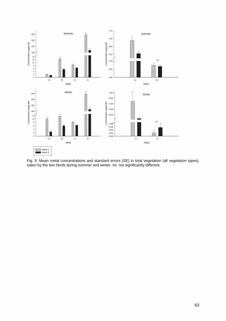
63
Summer
Metal
Cd Pb Cu Zn
Con
cent
ratio
n (µ
g/g
dw)
0
2
4
6
8
10
12
14
150
200
250
300 Summer
Metal
As Co
Con
cent
ratio
n (µ
g/g
dw)
0,00
0,05
0,10
0,60
0,80
1,00
1,20
ns
Winter
Metal
Cd Pb Cu Zn
Con
cent
ratio
n (µ
g/g
dw)
0
2
4
6
8
10
12
300
400
500
600 Winter
Metal
As Co
Con
cent
ratio
n (µ
g/g
dw)
0,000
0,002
0,004
0,006
0,008
0,200
0,400
0,600
0,800
1,000
ns
Herd 1 Herd 2
Fig. 5. Mean metal concentrations and standard errors (SE) in total vegetation (all vegetation types), eaten by the two herds during summer and winter. ns: not significantly different.
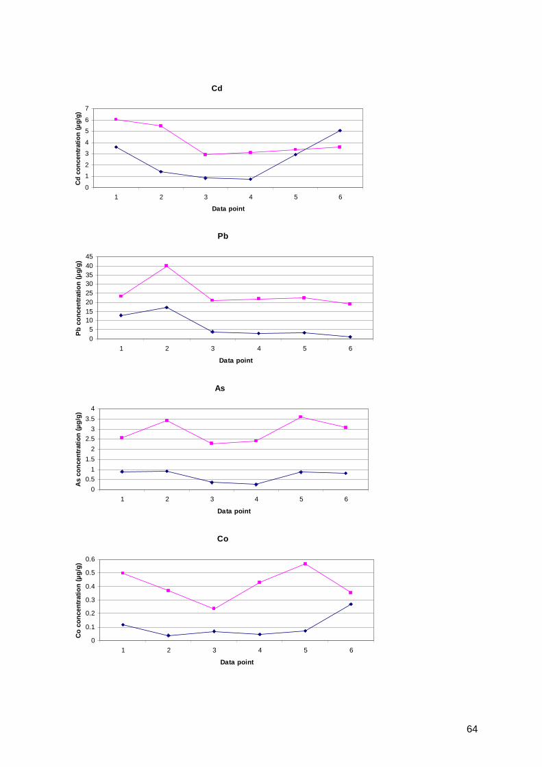
64
Cd
0
1
2
3
4
5
6
7
1 2 3 4 5 6
Data point
Cd
conc
entra
tion
(µg/
g)
Pb
05
1015202530354045
1 2 3 4 5 6
Data point
Pb
conc
entra
tion
(µg/
g)
As
0
0.5
1
1.5
2
2.5
3
3.5
4
1 2 3 4 5 6
Data point
As
conc
entr
atio
n (µ
g/g)
Co
0
0.1
0.2
0.3
0.4
0.5
0.6
1 2 3 4 5 6
Data point
Co
conc
entra
tion
(µg/
g)
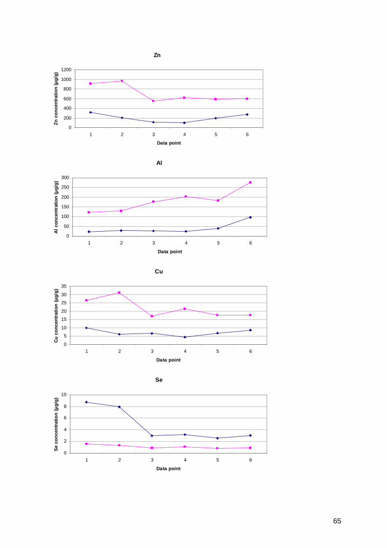
65
Zn
0
200
400
600
800
1000
1200
1 2 3 4 5 6
Data point
Zn
conc
entra
tion
(µg/
g)
Al
0
50
100
150
200
250
300
1 2 3 4 5 6
Data point
Al c
once
ntra
tion
(µg/
g)
Cu
0
5
10
15
20
25
30
35
1 2 3 4 5 6
Data point
Cu
conc
entra
tion
(µg/
g)
Se
0
2
4
6
8
10
1 2 3 4 5 6
Data point
Se
conc
entra
tion
(µg/
g)
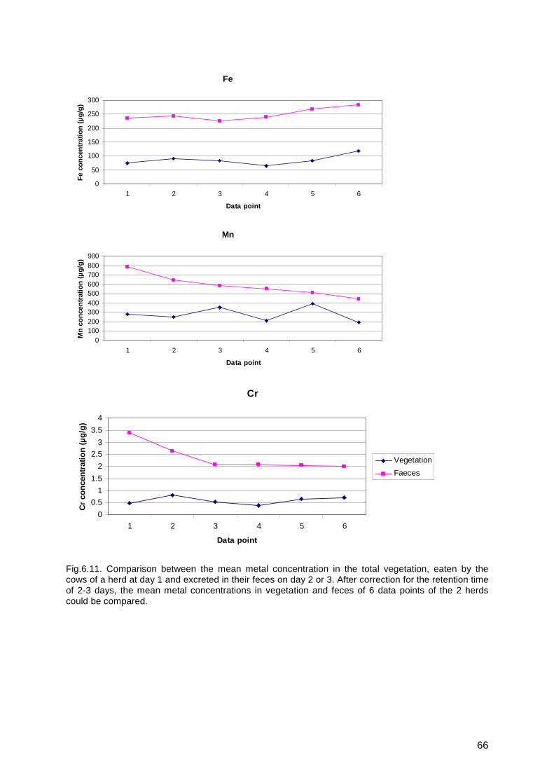
66
Fe
0
50
100
150
200
250
300
1 2 3 4 5 6
Data point
Fe
conc
entra
tion
(µg/
g)
Mn
0100200300400500600700800900
1 2 3 4 5 6
Data point
Mn
conc
entra
tion
(µg/
g)
Cr
0
0.5
1
1.5
2
2.5
3
3.5
4
1 2 3 4 5 6
Data point
Cr
conc
entra
tion
(µg/
g)
Vegetation
Faeces
Fig.6.11. Comparison between the mean metal concentration in the total vegetation, eaten by the cows of a herd at day 1 and excreted in their feces on day 2 or 3. After correction for the retention time of 2-3 days, the mean metal concentrations in vegetation and feces of 6 data points of the 2 herds could be compared.
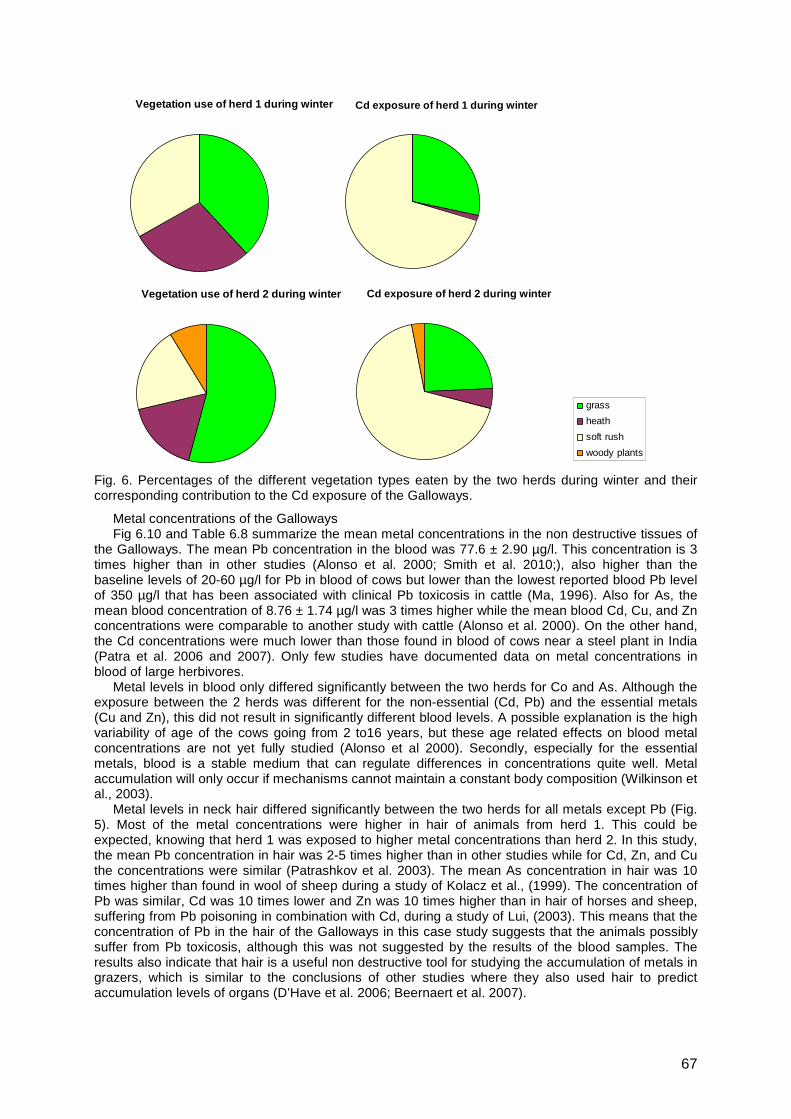
67
Vegetation use of herd 1 during winter Cd exposure of herd 1 during winter
Vegetation use of herd 2 during winter Cd exposure of herd 2 during winter
grass
heath
soft rush
woody plants
Fig. 6. Percentages of the different vegetation types eaten by the two herds during winter and their corresponding contribution to the Cd exposure of the Galloways.
Metal concentrations of the Galloways Fig 6.10 and Table 6.8 summarize the mean metal concentrations in the non destructive tissues of
the Galloways. The mean Pb concentration in the blood was 77.6 ± 2.90 µg/l. This concentration is 3 times higher than in other studies (Alonso et al. 2000; Smith et al. 2010;), also higher than the baseline levels of 20-60 µg/l for Pb in blood of cows but lower than the lowest reported blood Pb level of 350 µg/l that has been associated with clinical Pb toxicosis in cattle (Ma, 1996). Also for As, the mean blood concentration of 8.76 ± 1.74 µg/l was 3 times higher while the mean blood Cd, Cu, and Zn concentrations were comparable to another study with cattle (Alonso et al. 2000). On the other hand, the Cd concentrations were much lower than those found in blood of cows near a steel plant in India (Patra et al. 2006 and 2007). Only few studies have documented data on metal concentrations in blood of large herbivores.
Metal levels in blood only differed significantly between the two herds for Co and As. Although the exposure between the 2 herds was different for the non-essential (Cd, Pb) and the essential metals (Cu and Zn), this did not result in significantly different blood levels. A possible explanation is the high variability of age of the cows going from 2 to16 years, but these age related effects on blood metal concentrations are not yet fully studied (Alonso et al 2000). Secondly, especially for the essential metals, blood is a stable medium that can regulate differences in concentrations quite well. Metal accumulation will only occur if mechanisms cannot maintain a constant body composition (Wilkinson et al., 2003).
Metal levels in neck hair differed significantly between the two herds for all metals except Pb (Fig. 5). Most of the metal concentrations were higher in hair of animals from herd 1. This could be expected, knowing that herd 1 was exposed to higher metal concentrations than herd 2. In this study, the mean Pb concentration in hair was 2-5 times higher than in other studies while for Cd, Zn, and Cu the concentrations were similar (Patrashkov et al. 2003). The mean As concentration in hair was 10 times higher than found in wool of sheep during a study of Kolacz et al., (1999). The concentration of Pb was similar, Cd was 10 times lower and Zn was 10 times higher than in hair of horses and sheep, suffering from Pb poisoning in combination with Cd, during a study of Lui, (2003). This means that the concentration of Pb in the hair of the Galloways in this case study suggests that the animals possibly suffer from Pb toxicosis, although this was not suggested by the results of the blood samples. The results also indicate that hair is a useful non destructive tool for studying the accumulation of metals in grazers, which is similar to the conclusions of other studies where they also used hair to predict accumulation levels of organs (D’Have et al. 2006; Beernaert et al. 2007).
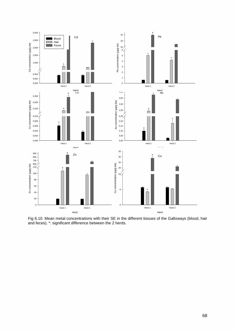
68
Fig 6.10. Mean metal concentrations with their SE in the different tissues of the Galloways (blood, hair and feces). *: significant difference between the 2 herds.
Co
Herd
Herd 1 Herd 2
Co
conc
enta
tion
(µg/
g dw
)
0,000
0,002
0,004
0,006
0,008
0,010
0,100
0,200
0,300
0,400
*
*
* As
Herd
Herd 1 Herd 2
As
conc
entr
atio
n (µ
g/g
dw)
0,00
0,05
0,10
0,15
0,20
0,25
1,00
2,00
3,00
4,00
*
*
*
Zn
Herd
Herd 1 Herd 2
Zn
conc
entr
atio
n (µ
g/g
dw)
0
20
40
60
80
100
120600
700
800
900
*
*Cu
Herd
Herd 1 Herd 2
Cu
conc
entr
atio
n (µ
g/g
dw)
0
5
10
20
25
30
35
*
*
Cd
Herd
Herd 1 Herd 2
Cd
conc
entr
atio
n (µ
g/g
dw)
0,000
0,002
0,004
1,000
2,000
3,000
4,000
5,000
*
*Pb
Herd
Herd 1 Herd 2
Pb
conc
entr
atio
n (µ
g/g
dw)
0
1
2
3
4
5
620
30
40*
Blood Hair Feces

69
Table 6.8. Mean metal concentrations with standard errors (SE) in the different tissues of the Galloways. Blood (µg/l or 10-3µg/g d.w.), hair and faeces (µg/g d.w.).
Tissue Blood (n=42) Hair (n=42) Faeces (n=131)
Metal
Mean ± SE Mean ± SE Mean ± SE Range Range Range
Ag
2.91 ± 0.521 0.017 ± 0.001 0.068 ± 0.050
0.012 - 11.8 0.007 - 0.045 6.05 x 10⁻⁵ - 6.49
Cd
3.43 ± 0.166 0.417 ± 0.031 4.11 ± 0.208 1.46 - 6.69 0.152 - 1.00 0.131 - 14.7
Pb
586 ± 22.3 4.49 ± 0.287 31.7 ± 1.07
304 - 1017 1.83 - 9.86 15.0 - 69.2
Al
166 ± 13.3 61.3 ± 3.89 160 ± 5.32
14.6 - 427 28.7 - 145 52.1 - 388
Cr
9800 ± 226 3.15 ± 0.028 2.75 ± 0.116
4697 - 13653 2.85 - 3.72 1.50 - 13.3
Mn
87.7 ± 9.94 8.13 ± 0.861 599 ± 13.1
26.9 - 419 1.29 - 25.9 301 - 1208
Fe
2674 ± 3 6.1 (mg/l) 67.8 ± 3.69 251 ± 4.04
1727 - 3111 (mg/l) 37.0 - 134 148 - 369
Co
5.76 ± 0.760 0.056 ± 0.004 0.380 ± 0.042
0.492 - 31.6 0.024 - 0.156 8.49 x 10⁻⁴ - 3.94
Ni
67.3 ± 45.4 0.149 ± 0.010 2.77 ± 0.085
4.19 - 1925 0.059 - 0.345 1.24 - 10.5
Cu
5664 ±141 4.63 ± 0.130 24.9 ± 0.873
2847 - 7388 3.09 - 6.48 11.1 - 61.9
Zn
19.2 – 0.431 (mg/l) 101 ± 2.66 759 ± 17.3
13.1 – 25.1 (mg/l) 63.1 - 154 442 - 1259
As
82.7 ± 14.8 0.561 ± 0.089 3.13 ± 0.161
9.40 - 470 0.003 - 1.98 1.76 - 20.7
In feces, the mean concentrations of Cd and Pb were respectively 10 and 3 times higher than those found in another study with steers (Gustafson & Olsson, 2004) and with horses although horses have another digestive system (Madejón et al. 2009). For As and Zn, the mean concentrations were comparable with those in the study with steers (Gustafson & Olsson, 2004). On the other hand, the Pb concentration was 3 times lower, Zn concentration 2 times higher and Cu concentration was similar than those in sheep feces (Smith et al. 2010). All metal concentrations in feces differed significantly between the two herds (Fig. 6.10). The differences in metal concentration can again be explained by the differences in metal exposure between the 2 herds. Animals of herd 1 were exposed to higher metal concentrations and this resulted in a higher metal excretion via feces. This suggests that a higher metal exposure not necessarily leads to an increase of the actual assimilation via the intestines. That is similar to earlier studies where they found that for example for Cd or Pb only 1-18% of the ingested metal concentration was assimilated (Miller et al. 1967; Lauwerys 1978, Tsuchiya K., 1979). In contrast, the absorption of essential metals such as Zn is much higher and can reach up to 50% of the total ingested concentration. There is no effective homeostatic protection against Pb absorption (Wilkinson et al., 2003). Lead is absorbed in the small intestine and transported in the erythrocytes where it replaces Fe in several enzymes concerned with hemoglobin production. When Cd is absorbed into the mucosal cells of the intestines, but not transferred to the bloodstream, it is bound to cell membranes and returns to the gastrointestinal tract. The absorption of many essential metals is controlled by homeostatic or homeorhetic mechanisms. Non-essential metals may use the absorption
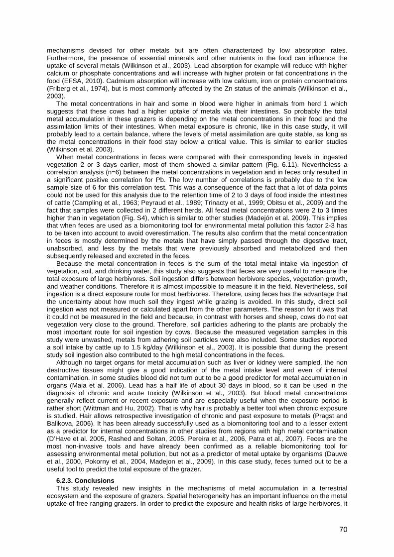
70
mechanisms devised for other metals but are often characterized by low absorption rates. Furthermore, the presence of essential minerals and other nutrients in the food can influence the uptake of several metals (Wilkinson et al., 2003). Lead absorption for example will reduce with higher calcium or phosphate concentrations and will increase with higher protein or fat concentrations in the food (EFSA, 2010). Cadmium absorption will increase with low calcium, iron or protein concentrations (Friberg et al., 1974), but is most commonly affected by the Zn status of the animals (Wilkinson et al., 2003).
The metal concentrations in hair and some in blood were higher in animals from herd 1 which suggests that these cows had a higher uptake of metals via their intestines. So probably the total metal accumulation in these grazers is depending on the metal concentrations in their food and the assimilation limits of their intestines. When metal exposure is chronic, like in this case study, it will probably lead to a certain balance, where the levels of metal assimilation are quite stable, as long as the metal concentrations in their food stay below a critical value. This is similar to earlier studies (Wilkinson et al. 2003).
When metal concentrations in feces were compared with their corresponding levels in ingested vegetation 2 or 3 days earlier, most of them showed a similar pattern (Fig. 6.11). Nevertheless a correlation analysis (n=6) between the metal concentrations in vegetation and in feces only resulted in a significant positive correlation for Pb. The low number of correlations is probably due to the low sample size of 6 for this correlation test. This was a consequence of the fact that a lot of data points could not be used for this analysis due to the retention time of 2 to 3 days of food inside the intestines of cattle (Campling et al., 1963; Peyraud et al., 1989; Trinacty et al., 1999; Obitsu et al., 2009) and the fact that samples were collected in 2 different herds. All fecal metal concentrations were 2 to 3 times higher than in vegetation (Fig. S4), which is similar to other studies (Madejón et al. 2009). This implies that when feces are used as a biomonitoring tool for environmental metal pollution this factor 2-3 has to be taken into account to avoid overestimation. The results also confirm that the metal concentration in feces is mostly determined by the metals that have simply passed through the digestive tract, unabsorbed, and less by the metals that were previously absorbed and metabolized and then subsequently released and excreted in the feces.
Because the metal concentration in feces is the sum of the total metal intake via ingestion of vegetation, soil, and drinking water, this study also suggests that feces are very useful to measure the total exposure of large herbivores. Soil ingestion differs between herbivore species, vegetation growth, and weather conditions. Therefore it is almost impossible to measure it in the field. Nevertheless, soil ingestion is a direct exposure route for most herbivores. Therefore, using feces has the advantage that the uncertainty about how much soil they ingest while grazing is avoided. In this study, direct soil ingestion was not measured or calculated apart from the other parameters. The reason for it was that it could not be measured in the field and because, in contrast with horses and sheep, cows do not eat vegetation very close to the ground. Therefore, soil particles adhering to the plants are probably the most important route for soil ingestion by cows. Because the measured vegetation samples in this study were unwashed, metals from adhering soil particles were also included. Some studies reported a soil intake by cattle up to 1.5 kg/day (Wilkinson et al., 2003). It is possible that during the present study soil ingestion also contributed to the high metal concentrations in the feces.
Although no target organs for metal accumulation such as liver or kidney were sampled, the non destructive tissues might give a good indication of the metal intake level and even of internal contamination. In some studies blood did not turn out to be a good predictor for metal accumulation in organs (Maia et al. 2006). Lead has a half life of about 30 days in blood, so it can be used in the diagnosis of chronic and acute toxicity (Wilkinson et al., 2003). But blood metal concentrations generally reflect current or recent exposure and are especially useful when the exposure period is rather short (Wittman and Hu, 2002). That is why hair is probably a better tool when chronic exposure is studied. Hair allows retrospective investigation of chronic and past exposure to metals (Pragst and Balikova, 2006). It has been already successfully used as a biomonitoring tool and to a lesser extent as a predictor for internal concentrations in other studies from regions with high metal contamination (D’Have et al. 2005, Rashed and Soltan, 2005, Pereira et al., 2006, Patra et al., 2007). Feces are the most non-invasive tools and have already been confirmed as a reliable biomonitoring tool for assessing environmental metal pollution, but not as a predictor of metal uptake by organisms (Dauwe et al., 2000, Pokorny et al., 2004, Madejon et al., 2009). In this case study, feces turned out to be a useful tool to predict the total exposure of the grazer.
6.2.3. Conclusions This study revealed new insights in the mechanisms of metal accumulation in a terrestrial
ecosystem and the exposure of grazers. Spatial heterogeneity has an important influence on the metal uptake of free ranging grazers. In order to predict the exposure and health risks of large herbivores, it
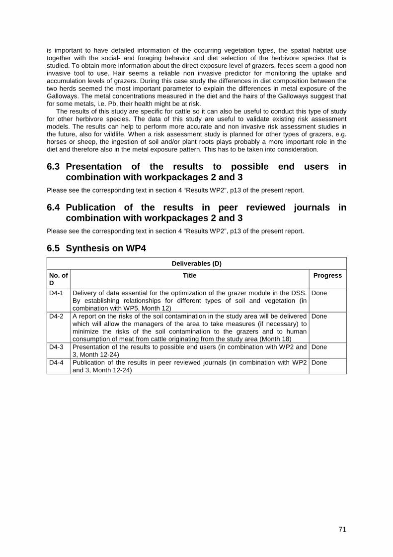
71
is important to have detailed information of the occurring vegetation types, the spatial habitat use together with the social- and foraging behavior and diet selection of the herbivore species that is studied. To obtain more information about the direct exposure level of grazers, feces seem a good non invasive tool to use. Hair seems a reliable non invasive predictor for monitoring the uptake and accumulation levels of grazers. During this case study the differences in diet composition between the two herds seemed the most important parameter to explain the differences in metal exposure of the Galloways. The metal concentrations measured in the diet and the hairs of the Galloways suggest that for some metals, i.e. Pb, their health might be at risk.
The results of this study are specific for cattle so it can also be useful to conduct this type of study for other herbivore species. The data of this study are useful to validate existing risk assessment models. The results can help to perform more accurate and non invasive risk assessment studies in the future, also for wildlife. When a risk assessment study is planned for other types of grazers, e.g. horses or sheep, the ingestion of soil and/or plant roots plays probably a more important role in the diet and therefore also in the metal exposure pattern. This has to be taken into consideration.
6.3 Presentation of the results to possible end use rs in combination with workpackages 2 and 3
Please see the corresponding text in section 4 “Results WP2”, p13 of the present report.
6.4 Publication of the results in peer reviewed jou rnals in combination with workpackages 2 and 3
Please see the corresponding text in section 4 “Results WP2”, p13 of the present report.
6.5 Synthesis on WP4
Deliverables (D)
No. of D
Title Progress
D4-1 Delivery of data essential for the optimization of the grazer module in the DSS. By establishing relationships for different types of soil and vegetation (in combination with WP5, Month 12)
Done
D4-2 A report on the risks of the soil contamination in the study area will be delivered which will allow the managers of the area to take measures (if necessary) to minimize the risks of the soil contamination to the grazers and to human consumption of meat from cattle originating from the study area (Month 18)
Done
D4-3 Presentation of the results to possible end users (in combination with WP2 and 3, Month 12-24)
Done
D4-4 Publication of the results in peer reviewed journals (in combination with WP2 and 3, Month 12-24)
Done
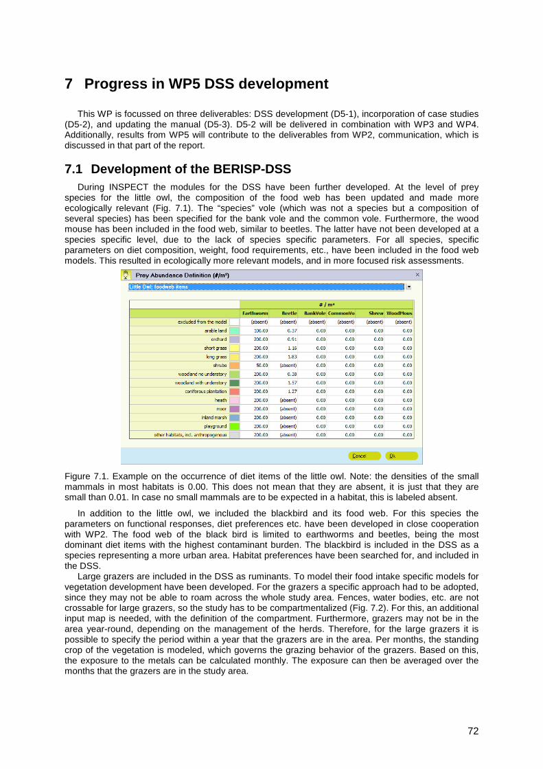
72
7 Progress in WP5 DSS development
This WP is focussed on three deliverables: DSS development (D5-1), incorporation of case studies (D5-2), and updating the manual (D5-3). D5-2 will be delivered in combination with WP3 and WP4. Additionally, results from WP5 will contribute to the deliverables from WP2, communication, which is discussed in that part of the report.
7.1 Development of the BERISP-DSS During INSPECT the modules for the DSS have been further developed. At the level of prey
species for the little owl, the composition of the food web has been updated and made more ecologically relevant (Fig. 7.1). The “species” vole (which was not a species but a composition of several species) has been specified for the bank vole and the common vole. Furthermore, the wood mouse has been included in the food web, similar to beetles. The latter have not been developed at a species specific level, due to the lack of species specific parameters. For all species, specific parameters on diet composition, weight, food requirements, etc., have been included in the food web models. This resulted in ecologically more relevant models, and in more focused risk assessments.
Figure 7.1. Example on the occurrence of diet items of the little owl. Note: the densities of the small mammals in most habitats is 0.00. This does not mean that they are absent, it is just that they are small than 0.01. In case no small mammals are to be expected in a habitat, this is labeled absent.
In addition to the little owl, we included the blackbird and its food web. For this species the parameters on functional responses, diet preferences etc. have been developed in close cooperation with WP2. The food web of the black bird is limited to earthworms and beetles, being the most dominant diet items with the highest contaminant burden. The blackbird is included in the DSS as a species representing a more urban area. Habitat preferences have been searched for, and included in the DSS.
Large grazers are included in the DSS as ruminants. To model their food intake specific models for vegetation development have been developed. For the grazers a specific approach had to be adopted, since they may not be able to roam across the whole study area. Fences, water bodies, etc. are not crossable for large grazers, so the study has to be compartmentalized (Fig. 7.2). For this, an additional input map is needed, with the definition of the compartment. Furthermore, grazers may not be in the area year-round, depending on the management of the herds. Therefore, for the large grazers it is possible to specify the period within a year that the grazers are in the area. Per months, the standing crop of the vegetation is modeled, which governs the grazing behavior of the grazers. Based on this, the exposure to the metals can be calculated monthly. The exposure can then be averaged over the months that the grazers are in the study area.
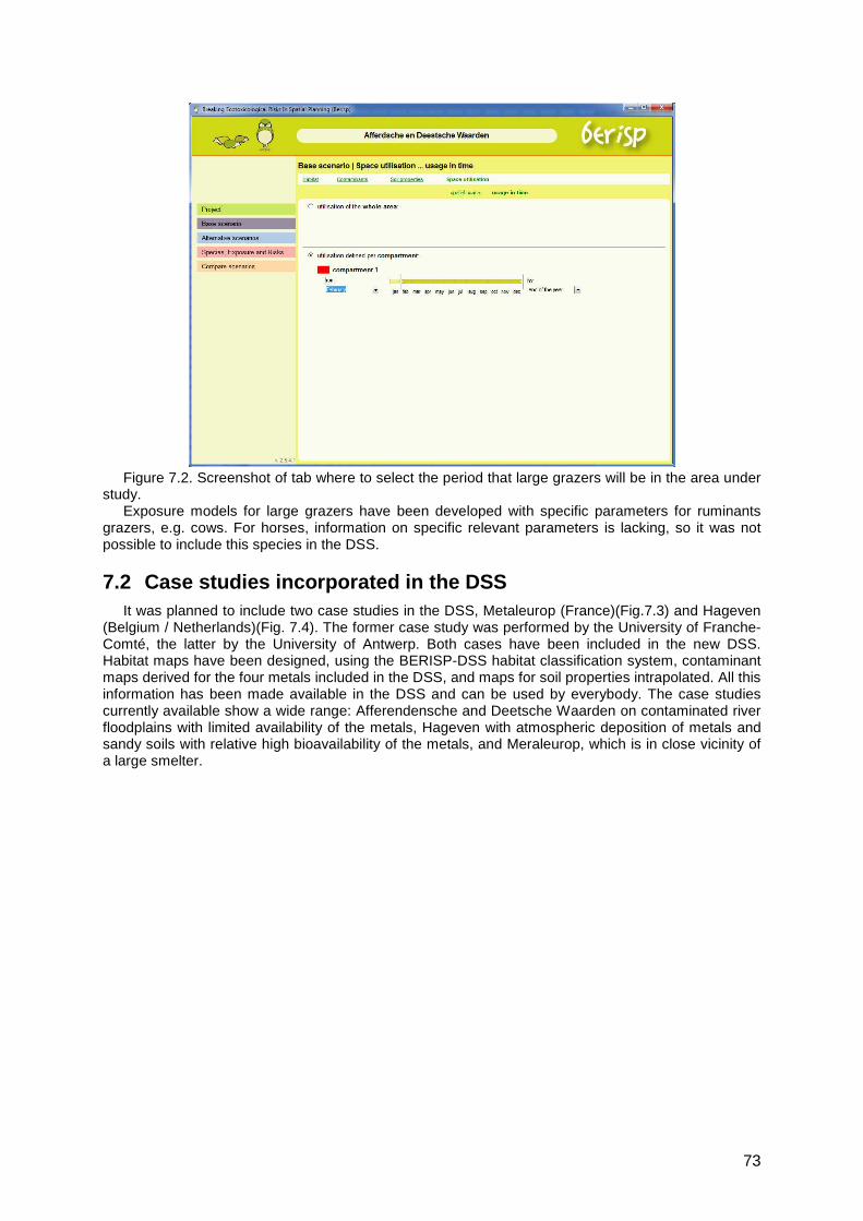
73
Figure 7.2. Screenshot of tab where to select the period that large grazers will be in the area under
study. Exposure models for large grazers have been developed with specific parameters for ruminants
grazers, e.g. cows. For horses, information on specific relevant parameters is lacking, so it was not possible to include this species in the DSS.
7.2 Case studies incorporated in the DSS It was planned to include two case studies in the DSS, Metaleurop (France)(Fig.7.3) and Hageven
(Belgium / Netherlands)(Fig. 7.4). The former case study was performed by the University of Franche-Comté, the latter by the University of Antwerp. Both cases have been included in the new DSS. Habitat maps have been designed, using the BERISP-DSS habitat classification system, contaminant maps derived for the four metals included in the DSS, and maps for soil properties intrapolated. All this information has been made available in the DSS and can be used by everybody. The case studies currently available show a wide range: Afferendensche and Deetsche Waarden on contaminated river floodplains with limited availability of the metals, Hageven with atmospheric deposition of metals and sandy soils with relative high bioavailability of the metals, and Meraleurop, which is in close vicinity of a large smelter.
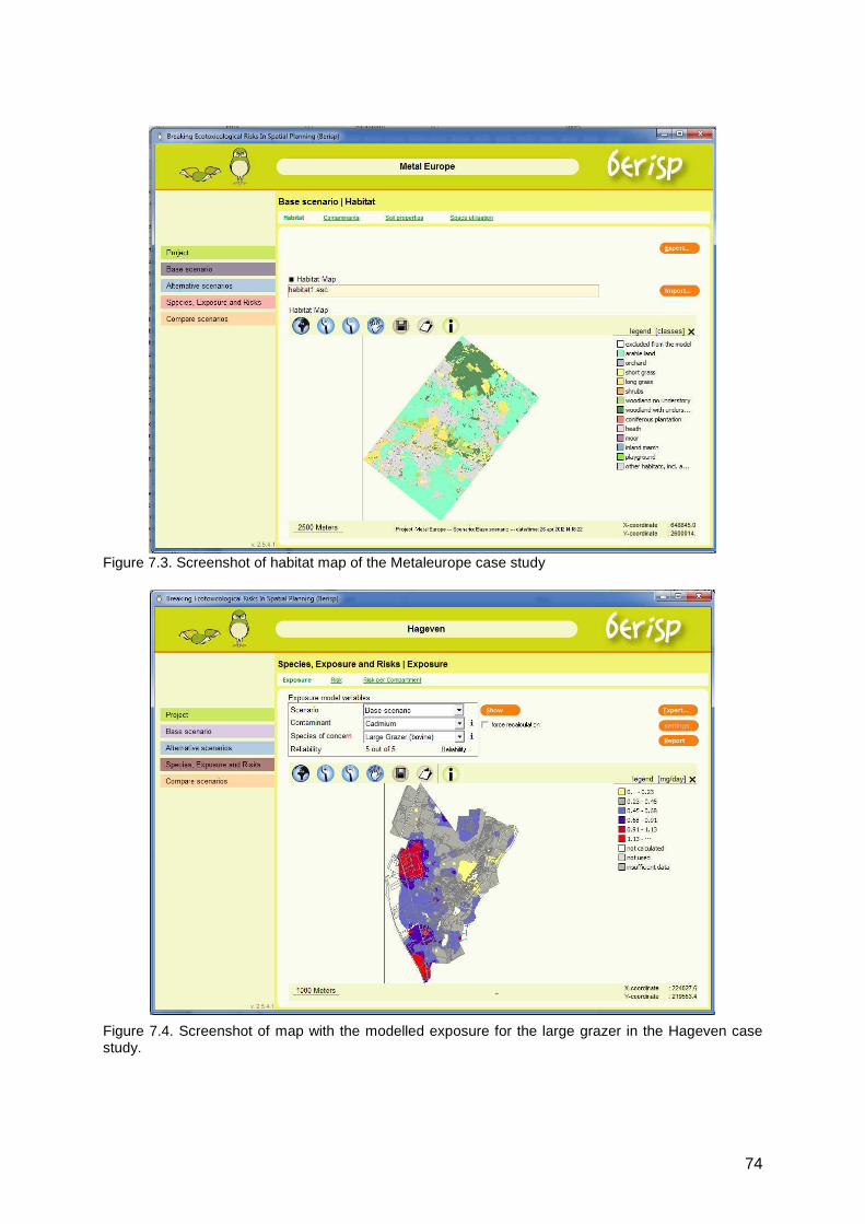
74
Figure 7.3. Screenshot of habitat map of the Metaleurope case study Figure 7.4. Screenshot of map with the modelled exposure for the large grazer in the Hageven case study.
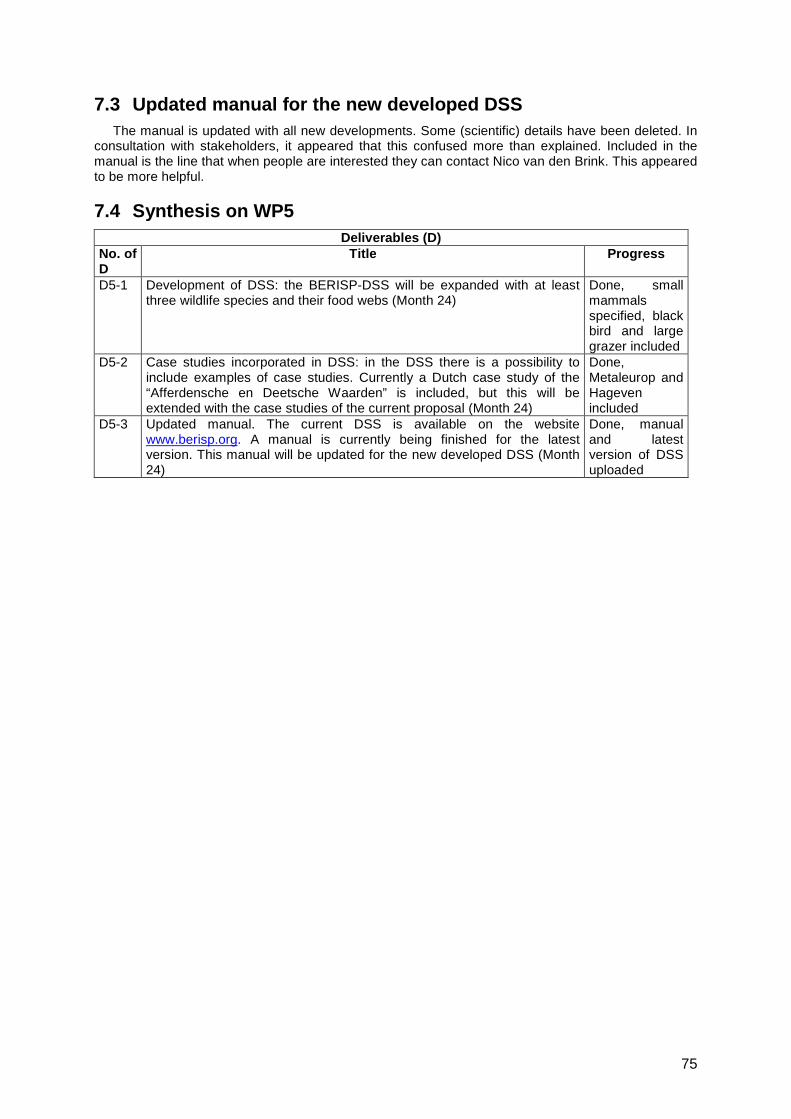
75
7.3 Updated manual for the new developed DSS The manual is updated with all new developments. Some (scientific) details have been deleted. In
consultation with stakeholders, it appeared that this confused more than explained. Included in the manual is the line that when people are interested they can contact Nico van den Brink. This appeared to be more helpful.
7.4 Synthesis on WP5 Deliverables (D)
No. of D
Title Progress
D5-1 Development of DSS: the BERISP-DSS will be expanded with at least three wildlife species and their food webs (Month 24)
Done, small mammals specified, black bird and large grazer included
D5-2 Case studies incorporated in DSS: in the DSS there is a possibility to include examples of case studies. Currently a Dutch case study of the “Afferdensche en Deetsche Waarden” is included, but this will be extended with the case studies of the current proposal (Month 24)
Done, Metaleurop and Hageven included
D5-3 Updated manual. The current DSS is available on the website www.berisp.org. A manual is currently being finished for the latest version. This manual will be updated for the new developed DSS (Month 24)
Done, manual and latest version of DSS uploaded
76
8 Application of results, conclusion and perspectiv es
The present programme allowed improving the BERISP-DSS that can now assess spatially the risk for the little owl, the European blackbird, and large grazers (cows), for Cd, Cu, Pb, and Zn, with three study cases (Afferdensche en Deetsche Waarden floodplain, Metaleurop Nord, Hageven-Plateaux reserve) dedicated to learn how to use the device. The device is of course usable for every site for which the environmental data (habitat, contamination, soil properties (optional)) needed to assess the risk are available. Data have been collected to add a new target species, the common kestrel.
As indicated by the different persons invited to BERISP-DSS presentation meetings, improvements could be made to enlarge the capabilities of the DSS and made it more spread and used. The following developments have been suggested by meeting participants: modules dedicated to human risk assessment, inclusion of indirect ecological effects (for instance, some pollutants may affect populations of preys that can have indirect effects on target health due to increasing competition for food, even if the pollutants do not affect them directly), integrated maps of risk for different target species in addition to the species-specific maps of the current version, development of aquatic modules, integration of bioavailability data based on laboratory bioassays or chemical extraction procedures, addition of measured data or maps of contamination in diet items (vegetation, earthworms, beetles, small mammals) if available on the study sites. Of course, implementing more pollutants and target species in the device has been encouraged. Moreover, some participants have also suggested developing BERISP-DSS as a collaborative project like the statistical software R (http://www.r-project.org), with possible contributions for all over the world. Some of those developments are currently in progress but most of them would need new funding to be achieved.
Efforts will be continued by the different scientific teams involved in INSPECT to improve the DSS and spread it within scientific and stakeholders communities.
9 References
Alonso M.L., Benedito J.L., Miranda M., Castillo C., Hernández J., Shore R.F. (2002a). Interactions between toxic and essential trace metals in cattle from a region with low levels of pollution. Archives of Environmental Contamination and Toxicology. 42: 165-172.
Alonso M.L., Benedito J.L. Miranda M., Castillo C., Hernández J., Shore R.F. (2002b). Cattle as biomonitors of soil Arsenic, copper, and zinc concentrations in Galicia (NW Spain). Archives of Environmental Contamination and Toxicology. 43: 103-108.
Alonso M.L., Benedito J.L., Miranda M., Castillo C., Hernández J., Shore R.F. (2000). Arsenic, cadmium, lead, copper and zinc in cattle from Galicia, NW Spain. The Science of the Total Environment. 246: 237-248.
Altmann J. (1974). Observational study of behaviour: sampling methods. Behaviour. 49: 227-267. Baumont R., Prache S., Meuret M., Morhand F.P. (2000). How forage characteristics influence
behaviour and intake in small ruminants: a review. Livestock Production Science. 61(1): 15-28. Beernaert J., Scheirs J., Leirs H., Blust R., Verhagen R. (2007). Non-destructive pollution exposure
assessment by means of wood mice hair. Environmental Pollution. 145: 443-451. Beresford N.A., Mayes R.W., Crout N.M.J., Maceachern P.K., Dodd B.A., Barnett C.L., Lamb C.S.
(1999). Transfer of cadmium and mercury to sheep tissues. Environmental Science & Technology. 33(14): 2395-2402.
Blust R., Van der Linden A., Verheyen E., Decleir W. (1988). Evaluation of microwave heating digestion and graphite furnace atomic absorption spectrometry with continuum source background correction for the determination of iron, copper and cadmium in brine shrimp. Journal of Analytical and Atomic Spectrometry. 3: 387–393.
Briggs H.M., Briggs D.M. (1980). Modern Breeds of Livestock. Fourth Edition, Macmillan Publishing Co.
Burnham, K., Anderson, D. (2002). Model Selection and Multi-model Inference. Springer-Verlag, New York, NY, USA.
Cai Q., Long M.L., Zhu M., Zhou Q.Z., Zhang L., Liu J. (2009). Food transfer of cadmium and lead to cattle in a lead-zinc smelter in Guizhou, China. Environmental Pollution. 157(11): 3078-3082.
Campling R.C., Freer M., Balch C.C. (1963). Factors affecting the voluntary intake of food by cows. 6: A Preliminary experiment with ground, pellet hay. British Journal of Nutrition. 17: 263-227.
Celechovska O., Malota S., Zima S. (2008). Entry of metals into food chains: a 20 year comparison
77
stydy in northern Maravia (Czech Republic), Acta Veterinaria Brno. 77: 654-652. Cramp, S. (1988). The Birds of the Western Palearctic. Volume 5: Tyrant Flycatchers to Thrushes.
Cramp, S. (ed). Oxford University Press, New York, USA. Crout N.M.J., Beresford N.A., Dawson J.M., Soar J., Mayes R.W. (2004). The transfer of As-73, Cd-
109 and Hg-203 to milk and tissues of dairy cattle. Journal of Agricultural Science. 142: 203-212. D’Havé H., Scheirs J., Mubiana V.K., Verhagen R., Blust R., De Coen W. (2005). Non-destructive
pollution exposure assessment in the European hedgehog (Erinaceus europaeus): I. Relationships between concentrations of metals and As in hair, spines and soil. Environmental Toxicology and Chemistry. 24: 2356-2364.
D’Havé H., Scheirs J., Mubiana V.K., Verhagen R., Blust R., De Coen W. (2006). Non-destructive pollution exposure assessment in the European hedgehog (Erinaceus europaeus): II. Hair and spines as indicators of endogenous metal and As concentrations. Environmental Pollution. 142: 438-448.
Dauwe T., Bervoets L., Blust R., Pinxten R., Eens M. (2000). Can excrements and feathers of nestling songbirds be used as biomonitors for heavy metal pollution? Archives of Environmental Contamination and Toxicology. 39: 541-546.
de Vries W., Römkens P.F.A.M, Bonten L.T.C. (2008). Spatially explicit integrated risk assessment of present soil concentrations of cadmium, lead, copper and zinc in The Netherlands. Water Air Soil Pollution. 191: 199-215.
Du Laing G., Rinklebe J., Vandecasteele B., Meers E., Tack F. M. G. (2009). Heavy metal mobility and availability in estuarine and riverine floodplain soils and sediments: a review. The Science of the Total Environment. 407: 3972-3985.
EFSA (European Food Safety Authority) (2010). Selected trace and ultratrace elements: Biological role, content in feed and requirements in animal nutrition – Elements for risk assessment. Technical report submitted to EFSA.
European Commission (2002). Directive 2002/32/EC of the European parliament and the council of 7 may 2002 on undesirable substances in animal feed. Official Journal of the European Community. L140: 10-21.
Fanrong Z., Shafaqat A., Haitao Z., Younan O., Boyin Q., Feibo W., Guoping Z. (2011). The influence of pH and organic matter content in paddy soil on heavy metal availability and their uptake by rice plants. Environmental Pollution. 159: 84-91.
Felius M. (1996). Rundvee, Rassen van de wereld. Misset Uitgeverij, Doetinchem, NL. 35: 48-51. Franz E., Romkens P., van Raamsdonk L., Van Der Fels-Klerx I. (2008). A chain modeling approach to
estimate the impact of soil cadmium pollution on human dietary exposure. Journal of Food Protection. 71(12): 2504-2513.
Friberg L., Piscator M., Nordberg G.F., Kjellström T. (1974). Cadmium in the environment. CRC Press, Cleveland.
Fritsch C., Cœurdassier M., Giraudoux P., Raoul F., Douay F., Rieffel D., de Vaufleury A., Scheifler R., (2011). Spatially Explicit Analysis of Metal Transfer to Biota: Influence of Soil Contamination and Landscape. PLoS ONE. 6(5): e20682.
Fritsch, C., Giraudoux, P., Coeurdassier, M., Douay, F., Raoul, F., Pruvot, C., Waterlot, C., de Vaufleury, A., Scheifler, R. (2010). Spatial distribution of metals in smelter-impacted soils of woody habitats: influence of landscape and soil properties, and risk for wildlife. Chemosphere. 81: 141-155.
Grant R.J., Albright J.L. (2001). Effect of Animal grouping on feeding behavior and intake of dairy cattle. Journal of Dairy Science. 84(E. Suppl.): E156-E163.
Gustafson G.M., Olsson I. (2004). Partitioning of nutrient and trace elements in feed between body retention, faeces and urine by growing dairy-breed steers. Acta Agric. Scand., Sect. A, Animal Science. 54: 10-19.
Heikens, A., Peijnenburg, W., Hendriks, A. (2001). Bioaccumulation of heavy metals in terrestrial invertebrates. Environmental Pollution. 113: 385-393.
Heiri O, Lotter AF, Lemcke G. (2001). Loss on ignition as a method for estimating organic and carbonate content in sediments: reproducibility and comparability of results. Journal of Paleolimnology. 25: 101-110.
Hicks R.B., Owens F.N., Gill D.R., Oltjen J.W., Lake R.P. (1990). Daily dry matter intake by feedlot cattle: influence of breed and gender. Journal of Animal Science. 68: 245-253.
Hou L.Y., Shi W.M., Wei W.H., Shen H. (2011). Cadmium uptake, translocation, and tolerance in AHA1OX Arabidopsis thaliana. Biological Trace Element Research. 139: 228-240.
Impellitteri C.A., Lu Y. F., Saxe J.K., Allen H. E., Peijnenburg W. J. G. M., (2002). Correlation of the partitioning of dissolved organic matter fractions with the desorption of Cd, Cu, Ni, Pb and Zn from
78
18 Dutch soils. Environment International. 28: 401-410. Johnson C.R., Lalman D.L., Brown M.A., Appeddu L.A., Buchanan D.S., Wettermann R.P. (2003).
Influence of milk production potential on forage dry matter intake by multiparous and primiparous Brangus females. Journal of Animal Science. 81: 1837-1846.
Jumba I.O., Kisia S.M., Kock R. (2007). Animal health problems attributed to environmental contamination in lake Nakuru National Park, Kenya: A case study on heavy metal poisoning in the waterbuck Kobus ellipsiprymnus defassa (Ruppel 1835). Archives of Environmental Contamination and Toxicology. 52: 270-281.
Kabata-Pendias, A. (2000). Trace elements in soils and plants. CRC Press, Boca Raton, FL, USA. Kolacz R., Bodak E., Dobrzanski Z., Patkowska-Sokola B. (1999). Trace elements in the wool of
Polish merino sheep grazed in polluted and unpolluted environment. Czech Journal of Animal Science. 44(11): 509-514.
Kramarova M., Massanyi P., Slamecka J., Tataruch F., Jancova A., Gasparik J., Fabis M. Kovacik J., Toman R., Galova J., Jurcik R. (2005). Distribution of cadmium and lead in liver and kidney, of some wild animals in Slovakia. Journal of Environmental Science and Health Part A-Toxic/Hazardous Substances & Environmental Engineering. 40(3): 593-600.
Lauwerys R.R. (1978). Criteria (dose/effect relationships) for Cadmium. Report of a working group of experts prepared for the commission of the European Communities, Directorate-General for Social Affairs, Health and Safety Directorate. Pergamon, Oxford, pp.126.
Liu Z.P. (2003). Lead poisoning combined with cadmium in sheep and horses in the vicinity of non-ferrous metal smelters. The Science of the Total Environment. 309: 117-126.
Lusky K., Bohm D., Stoyke M., Hecht H., Luthardt M., Lippert A. (1992). Studies in environmental contaminants in wild boars, red deer, roe deer, moufflon and fallow deer from the biosphere reservation Schorfheide-Chorin. Archives Fur Lebensmittelhygiene. 43(6): 131-136.
Ma W.C. (1996). Chapter 12: Lead in Mammals, in: Beyer W.N., Heinz G.H., Redmon-Norwood A.W. (Eds), Environmental Contaminants in Wildlife, Interpreting Tissue Concentrations. Lewis Publishers, CRC Press LLC, pp. 281-296.
Madejón P., Dominguez M.T., Murillo J.M., (2009). Evaluation of pastures for horses grazing on soils polluted by trace elements. Ecotoxicology. 18: 417-428.
Maia L., De Souza M.V., Fernandes R.B.A., Fontes M.P.F., Vianna M.W., Luz W.V. (2006). Heavy metals in Horse blood, serum and feed in Minas Gerais, Brazil. Journal of Equine veterinary Science. 26(12): 578-583.
Malandrino M., Abollino O. Buoso S. Giacomino A., La Gioia C., Mentasti E. (2011). Accumulation of heavy metals from contaminated soil to plants and evaluation of soil remediation by vermiculite. Chemosphere. 82: 169-178.
Martin P. and Bateson P. (2007). Measuring Behaviour: An Introductory Guide. 3rd edition. Cambridge: Cambridge University Press.
Massanyi P., Tataruch F., Slameka J., Toman R., Juric R., (2003). Accumulation of lead, cadmium and mercury in liver and kidney of the brown hare (Lepus europaeus) in relation to the season, age and sex in the west Slovakian lowland. Journal of Environmental Science and Health Part A-Toxic/Hazardous Substances & Environmental Engineering. 38(7): 1299-1309.
Mester Z., Sturgeon R. (2003). Sample preparation for trace metal analysis. 41: 943-944. Miller W.J., Lampp B., Powell G.W., Salotti C.A., Blackmon D.M. (1967). Influence of a high level of
dietary cadmium on cadmium content in milk, excretion and cow performance. Journal of Dairy Science. 50: 1404-1408.
Mor F., Sonal S., Cerit H. (2005). Lead and cadmium levels in tissues of horses in Bursa, Turkey. Fresenius Environmental Bulletin. 14(9): 773-776.
Obitsu T., Goto M., Sugino T., Taniguchi K., Yukizane K., Imoto S., Yanagawa M., El-Sabagh M. (2009). The effect of dietary ratios of corn silage and alfalfa hay on carbohydrate digestion and retention time of feed particles in the gastrointestinal tract of steers. Animal Science Journal. 80: 546-555.
OVAM (2008). Scenario's voor het beheer en sanering van de grensoverschrijdende bodemverontreiniging in de Kempen. Samenvatting van het symposium BeNeKempen van 23 juni 2008.
Parkpian P., Leong S.T., Laortanakul P., Thunthaisong N., (2002). Regional monitoring of lead and cadmium contamination in a tropical grazing land site, Thailand. Environmental Monitoring and Assessment. 85: 157-173.
Patra R.C., Swarup D., Naresh R., Kumar P., Nandi D., Shekhar P., Roy S. Ali S.L. (2007). Tail hair as an indicator of environmental exposure of cows to lead and cadmium in different industrial areas. Ecotoxicology and Environmental Safety. 66: 127-131.
79
Patra R.C., Swarup D., Sharma M.C., Naresh R. (2006). Trace mineral profile in blood and hair from cattle exposed to lead and cadmium around different industrial units. Journal of Veterinary Medicine. 53: 511-517.
Patrashkov S.A., Petukhov V.L., Korotkevich O.S., Petukhov I.V. (2003). Content of heavy metals in the hair. Journal De Physique IV. 107: 1025-1027.
Pereira R., Pereira M., Ribeiro R., Goncalves F. (2006). Tissues and hair residues and histopathology in wild rats (Rattus rattus L.) and Algerian mice (Mus spretus Lataste) from an abandoned mine area (southeast Portugal). Ecotoxicology and Environmental Safety. 43(2): 561-575.
Peyraud J.L., Mambrini M., Rulquin H. (1989). Transit time measured by rare earth elements in dairy cows fed with three diets offered at two levels of feed intake. Asian-Australian Journal of Animal Sciences. 2(3): 366-367.
Ping Z., Huiling Z., Wensheng S. (2009). Biotransfer of heavy metals along a soil-plant-insect-chicken food chain: Field study. Journal of Environmental Sciences. 21: 849-853.
Pokorny B., Al Sayegh-Petkovsek S., Ribaric-Lasnik C., Vrtacnik J., Doganoc D.Z., Adamic M. (2004). Fungi ingestion as an important factor influencing heavy metal intake in roe deer: evidence from faeces. The Science of the Total Environment. 324: 223-234.
Pragst F., Balikova M. (2006). State of the art in hair analysis for detection of drug and alcohol abuse. Clinica Chimica Acta. 370(1-2): 17-49.
Queralt I., Barreiros M.A., Carvalho M.L., Costa M.M. (1999). Application of different techniques to assess sediment quality and point source pollution in low-level contaminated estuarine recent sediments (Lisboa coast, Portugal). The Science of the Total Environment. 241: 39-51.
R Development Core Team 2012. (2012). R: a language and environment for statistical computing. Vienna, Austria.
Rascio N., Navari-Izzo F. (2011). Heavy metal hyperaccumulating plants: How and why do they do it? And what makes them so interesting? Plant Science. 180: 169-181.
Rashed M., Soltan M. (2005). Animal hair as biological indicator for heavy metal pollution in urban and rural areas. Environmental Monitoring and Assessment. 110(1-3): 41-53.
Reglero M.M., Monsalve-González L., Taggart M.A., Mateo R. (2008). Transfer of metals to plants and red deer in an old lead mining area in Spain. The Science of the Total Environment. 406: 287-297.
Rhind S.M., Kyle C.E., Owen J. (2005). Accumulation of potentially toxic metals in the liver tissues of sheep grazed on sewage sludge-treated pastures. Animal Science. 81: 107-113.
Roberts A.H.C., Longhrst R.D., Brown M.W. (1994). Cadmium status of soil, plants, and grazing animals in New-Zealand. New Zealand Journal of Agricultural Research. 37(1): 119-129.
Römkens P.F.A.M., Guo H.Y, Chu C.L., Liu T.S., Chiang C.F., Koopmans G.F. (2009). Prediction of cadmium uptake by brown rice and derivation of soil-plant transfer to improve soil protection guidelines. Environmental Pollution. 157: 2435-2444.
Schulte-Hostedde, A., Millar, J., Hickling, G. (2001). Evaluating body condition in small mammals. Canadian Journal of Zoology. 79: 1021-1029.
Smith K.M., Abrahams P.W., Dagleish M.P., Steigmajer J. (2009). The intake of lead and associated metals by sheep grazing mining contaminated floodplain pastures in mid-Wales, UK: I. soil ingestion, soil-metal partitioning and potential availability to pasture herbage and livestock. The Science of the Total Environment. 407: 3731-3739.
Smith K.M., Dagleish M.P., Abrahams P.W. (2010). The intake of lead and associated metals by sheep grazing mining contaminated floodplain pastures in mid-Wales, UK: II. Metal concentrations in blood and wool. The Science of the Total Environment. 408: 1013-1042.
Somasundaram J, Krishnasamy R., Savithri P. (2005). Biotransfer of heavy metals in jersey cows. Indian Journal of Animal Sciences. 75(11): 1257-1260.
Sukreeyapongse O., Holm P.E., Strobel B.W., Panichsakpatana S., Magid J., Hansen H.C.B. (2002). pH-dependent release of cadmium, copper, and lead from natural and sludge-amended soils. Journal of Environmental Quality. 31: 1901-1909.
Swarup D., Patra RC., Naresh R., Kumar P., Shekkar P., Balagangatharathilagar M. (2006). Lowered blood copper and cobalt contents in goats reared around lead-zinc smelter. Small Ruminant Research. 63(3), 309-313.
Tack F.M., Verloo M.G. (1996). Metal concentrations in stinging nettle (Urtica dioica L.) as affected by soil characteristics. The Science of the Total Environment. 192: 31-39.
Tessier A., Campbell P.G.C., Auclair J.C., Bisson M. (1984). Relationships between the partitioning of trace metals in sediments and their accumulation in the tissues of the freshwater mollusc Elliptio complanata in a mining area. Canadian Journal of Fishery and Aquatic Sciences. 41: 1463-1472.
Theocharopoulos SP, Wagner G, Sprengart J, Mohr ME, Desaules A, Muntau H, Christou M, Quevauviller P. (2001). European soil sampling guidelines for soil pollution studies. The Science of
80
the Total Environment. 264: 51-62. Trinacty J., Simek M., Zeman L., Harazim J. (1999). Passage of large plastic particles trough the
digestive tract of lactating and dry cows. Journal of Animal and Feed Sciences. 8(2): 263-272. Tsuchiya K. (1979). Lead. In: Friberg L. Nordberg G.F., Vouk V.B. (eds) Handbook on the toxicology of
metals. Elsevier/North Holland Biomedical Press, Amsterdam, 451-482. USEPA. (2005). Guidance for developing ecological soil screening levels. 85. Van den Brink N., Lammertsma D., Dimmers W., Boerwinkel M., van der Hout A. (2010). Effects of soil
properties on food web accumulation of heavy metals to the wood mouse (Apodemus sylvaticus). Environmental Pollution. 158: 245-251.
Van den Brink N., Lammertsma D., Dimmers W., Boerwinkel M.C. (2011). Cadmium accumulation in small mammals: species traits, soil properties, and spatial habitat use. Environmental Science and Technology. 45: 7497-7502.
van Wezel A.P., de Vries W., Beek M., Otte P.F.M., Lijzen J.P.A., Mesman P.L.A., van Vlaardeingen A., Tuinstra J., van Elswijk M., Römkens P.F.A.M., Bonten L.T.C. (2003). Bodemgebruikswaarden voor landbouw, natuur en waterbodem. Technisch wetenschappelijke afleiding van getalwaarden, RIVM Rapport 711701031, pp. 33-35.
Van Wezel A.P., de Vries W., Beek M., Otte P.F.M., Lijzen J.P.A., Mesman M., van Vlaardingen P.L.A., Tuinstra J., van Elswijk M., Römkens P.F.A.M., Bonten L. (2003). Bodemgebruikswaarden voor landbouw, natuur en waterbodem. Technisch wetenschappelijke afleidingen van getalswaarden. RIVM rapport.
Veltman, K., Huijbregts, M.A.J., Hamers, T., Wijnhoven, S., Hendriks, A. J. (2007). Cadmium accumulation in herbivorous and carnivorous small mammals: Meta-analysis of field data and validation of the bioaccumulation model optimal modeling for ecotoxicological applications. Environmental Toxicology and Chemistry. 26: 1488-1496.
Vermeulen F., Van den Brink N., D’ Havé H., Mubiana V.K., Blust R., Bervoets L., De Coen W., (2009). Habitat type-based bioaccumulation and risk assessment of metal and As contamination in earthworms, beetles and woodlice. Environmental Pollution. 157: 3098-3105.
VLAREBO (2008). Besluit van de Vlaamse Regering houdende vaststelling van het Vlaams reglement betreffende de bodemsanering en de bodembescherming. Bijlage IV: Bodemsaneringnormen.
Wallis de Vries M.F., Daleboudt C. (1994). Foraging strategy of cattle in patchy grassland. Oecologia. 100: 98-106.
Wang S.P., Wang Y.F., Hu Z.Y., Chen Z.Z., Fleckenstein J., Schnug E. (2003). Status of iron, manganese, copper and zinc of soils and plants, and their requirement for ruminants in Inner Mongolia steppes of China. Communications in Soil Science and Plant Analysis. 34(5-6): 655-670.
Wilkinson J.M., Hill J., Phillips C.J.C. (2003). The accumulation of potentially-toxic metals by grazing ruminants. Proceedings of the Nutrition Society. 62(2): 267-277.
Wittman R., Hu H. (2002). Cadmium exposure and nephropathy in a 28-year old female metals worker. Environmental Health Perspectives. 10(12): 1261-1266.
Yusuf M., Fariduddin Q., Hayat S., Ahmad A. (2011). Nickel: an overview of uptake, Essentiality and toxicity in plants. Bulletin of Environmental Contamination and Toxicology. 86: 1-17.