INSTITUTO DE CIBERNETICA MATEMATICA Y FISICA

AN APPROXIMATE INNOVATION METHOD FOR THE ESTIMATION OF DIFFUSION PROCESSES

FROM DISCRETE DATA

J.C. Jimenez and T. Ozaki

October 2002 ICIMAF 2002-184

Centro de Matemática y Física Teórica Calle E #309 esq. a 15, Vedado, Ciudad de La Habana, C.P. 10400, Telef: 331-3354, 31-3432, Fax: (537) 33 3373, Telex: 51 2230 ICIMAF CU

AN APPROXIMATE INNOVATION METHOD FOR THEESTIMATION OF DIFFUSION PROCESSES FROM

DISCRETE DATA

J.C. Jimenez and T. OzakiInstituto de Cibernética, Matemática y Física,

Apartado Postal 6020, Zona Postal 6, La Habana, CubaThe Institute of Statistical Mathematics,

4-6-7 Minami-Azabu, Minato-ku, Tokyo 106-8569, Japan

Abstract

In this paper an approximate innovation method is introduced for the estimation ofdiffusion processes given a set of discrete and noisy observations of some of their components.The method is based on a recent extension of Local Linearization filters to the general caseof continuous-discrete state space models with multiplicative noise. This filtering methodprovides adequate approximations for the prediction and filter estimates that are requiredby the innovation method in the estimation of the unknown parameters and the unobservedcomponent of the diffusion process. The performance of approximate innovation estimatorsis illustrated by means of numerical simulations.

1 Introduction

Diffusion processes form a large class of continuous time processes that have been widely used forthe stochastic modeling of dynamical phenomena in physical, engineering, social and life sciences.Statistical inference for diffusion processes is thus of great importance from the theoretical aswell as from the applied point of view in model building and model selection. During the last 20years, much progress has been made in the study of parameter estimation for diffusion processeswhen the processes have been continuously or discretely observed over a period of time. Anupdated and detailed review of these inference techniques is given in Prakasa Rao (1999).

Typically it is assumed in theoretical studies that all the components of the diffusion processesare (continuously or discretely) observed. However, this is generally not the case in practicalapplications. For instance, the α rhythm of a human electroencephalogram recorded at a pointon the scalp is described by multidimensional neural mass models (Valdes et al., 1999) and, infinance, the stock price dynamics may be described by multidimensional stochastic volatilitymodels (Ghysels et al., 1996). Moreover, in practical applications as mentioned above, an addi-tional difficulty usually appears: the observations are contaminated with measurement noise.

This paper is concerned with the class of inference problems in which the parameters of adiffusion process must be estimated from discrete and noisy observations of some of its com-ponents. In this case, the inference problem for diffusion processes could be reformulated in anatural way using the framework of continuous-discrete state space models (see, e.g., models(1)-(2)). In Schweppe (1965) the maximum likelihood estimator for linear models with additivenoise has been considered and two forms for evaluating the likelihood function were also proposed(see also Singer (1993) and references therein for alternatives ways of evaluating the likelihood

1

function in that model). Recently, in Jensen & Petersen (1999), the asymptotic normality of themaximum likelihood estimators for state space models has been studied. A second inferentialmethod, based on an innovation approach, has been proposed in Ozaki (1994). In this method,the innovation estimators are obtained by minimizing a certain function of the prediction errors,where the predictions are obtained from the solution of the filtering problem associated withthe continuous-discrete state space model. Because the exact computation of the predictionsin a filtering problem is only possible in a few non-trivial cases (see, e.g., Brigo & Hanzon,1998; Geyer & Pichler, 1996), some approximations must be made. In Ozaki (1994), Jimenez(1996) and Shoji (1998) the predictions are approximated by using different kinds of Local Lin-earization (LL) filters. The satisfactory performance of this approximate innovation methodhas been demonstrated through various simulation studies (Ozaki, 1994; Shoji, 1998; Ozaki etal., 2000) and, also, through its successful application to the simultaneous estimation of theunknown parameters and the unobserved components of a neurophysiological model from actualEEG data (Valdes et al., 1999) and a HIV-AIDS epidemic model from actual data (Pedroso etal., 2003). However, the method is restricted to state space models with additive noise becausethe limitations of the LL filter itself. For models with multiplicative noise, the predictions ofthe innovation estimators have been approximated by using the extended Kalman filter (Nielsenet al., 2000a) and second order filters (Nielsen et al., 1998, 2000c). In Nielsen et al. (2000c),these approximate innovation methods have been applied for the simultaneous estimation of theunknown parameters and the unobserved components of several stochastic volatility models. Inthat study unbiased estimates for the parameters were reported, but also large biased estimatesfor some unobserved components of the process. However, the main drawback of these approxi-mate estimators is that the filters used by them are computational unstable for diverse types ofnonlinear problems. This instability often becomes visible as a numerical explosion in the com-putation of the prediction or filtering estimates at an instant of time (Ozaki, 1993). Recentlyin Nolsoe et al. (2000), an alternative inferential method has been considered. In that paper,the prediction-based estimating functions method introduced in Soerensen (2000) is analyzed indetail for the case of observations corrupted with additive noise. In contrast to the innovationmethod, this estimating function method involves unconditional moments, does not explicitlytreat the estimation of unobserved components of the process and, often, needs the computationof the unconditional moments and their derivatives by Monte Carlo simulations, which might betime-consuming (Nolsoe et al. 2000).

In this paper, the approximate innovation method based on the LL filters is reconsidered.Specifically, the method is extended to diffusion processes with multiplicative noise and nonlin-ear observations. This has been made possible because of: 1) the recent extension of LL filters tothe general case of continuous-discrete state space models with multiplicative noise (Jimenez &Ozaki, 2003), which is a stable and efficient alternative to the other filter approximations men-tioned above; and 2) the extension of the innovation method to the case of nonlinear observationsintroduced in this paper.

The paper is organized as follows. In section 2, a precise formulation of the innovationapproach is presented, which includes the original method for models with linear observationsand its extension to models with nonlinear observations. In section 3, the approximate innovationmethod based on the LL filter is introduced and, in the last section, the performance of thatapproximate estimator is illustrated by mean of simulations.

2

2 The innovation approach

2.1 Models with linear observations

Let the state space model be defined by the continuous state equation

dx(t) = f(t,x(t);α)dt+mXi=1

gi(t,x(t);α)dwi(t), for t ≥ t0 ∈ R, (1)

and the discrete observation equation

ztk = Cx(tk) + etk , for k = 0, 1, .., N ∈ N, (2)

where x(t) ∈ Rd is the state vector at the instant of time t, ztk ∈ Rr is the observation vector atthe instant of time tk, α is a set of parameters, w is an m-dimensional standard Wiener process,{etk : etk ∼ N (0,Σ), k = 0, ..,N} is a sequence of i.i.d. random vectors independent of w, Cis a r × d constant matrix, and f , gi : R × Rd → Rd are nonlinear vector functions. Here, thetime discretization (t)N = {tk : k = 0, 1, · · · , N} is assumed to be increasing, i.e., tk−1 < tk forall k = 1, .., N .

Let xt/tk = E(x(t)/Ztk ;α) and Pt/tk = E((x(t) − xt/tk)(x(t) − xt/tk)|/Ztk ;α) for all t ≥ tk,where E(./.) denotes conditional expectation and Ztk = {ztj : tj ≤ tk and tj ∈ (t)N} is asequence of observations. In the case that t > tk, xt/tk and Pt/tk are called prediction andprediction variance, respectively. If t = tk, xtk/tk and Ptk/tk are called filter and filter variance.Let ϑ = {xt0/t0 ,Pt0/t0 , α}.

In a model like (1)-(2) with ϑ given, the problem of estimating the state x(tk) from theobservations Ztk is known as the continuous-discrete filtering problem. The major contributionto the solution of this problem is due to Kalman (1960) and Kalman & Bucy (1961), who provideda sequential and efficient method of computing xt/tk for the case where f and gi are linear andconstant functions, respectively. In the general case, the solution is also well known, althoughit usually does not have explicit form and good approximations are required (Jazwinski, 1970).In this framework, the discrete-time innovation process {νtk : k = 1, .., N} defined as

νtk = ztk −Cxtk/tk−1

has played an important theoretical role (see Kailath, 1974 & 1991 for details).More recently, this innovation process has also been useful for the estimation of ϑ in model

(1)-(2). The inference method, introduced in Ozaki (1994), is based on the following threeobservations related with that process:

1. In continuous filtering problems with observations dz(t) = κ(t)dt + d$(t) and initial

condition z(0) = 0, progressively measurable process κ such that E(tR0

|κ(s)| ds) < ∞, and

Wiener process $, the continuous-time innovation process {υ(t) : t ≥ 0} defined by

υ(t) = z(t)−tZ0

κ(s)ds, with κ(t) =E(κ(t)/{z(s) : s ≤ t})

is a Wiener process. (Kailath 1971, Theorem 2; Kallianpur 1980, Corollary 8.1.1).2. νtk → dυ(tk) as ∆→ 0, where ∆ = max{tk−tk−1}k=1,..,N (Kailath 1981, p. 99). This and

observation 1) imply that the distribution of the random vector νtk is approximately Gaussian,for ∆ sufficiently small.

3

3. Assuming Gaussianity for νtk , the likelihood function expressed as the product of condi-tional densities by

L(ϑ;ZtN ) =NYi=1

p(νtk/Ztk−1 , ϑ)

is completely characterized by the conditional first and second order moments

νtk/tk−1 = E(νtk/Ztk−1 ;ϑ) = 0,

andΣνtk/tk−1 = E((νtk − νtk/tk−1)(νtk − νtk/tk−1)

|/Ztk ;ϑ) = CPtk/tk−1C| +Σ,

respectively. Here, p(νtk/Ztk−1 , ϑ) denotes the multivariate Gaussian pdf with zero mean andvariance Σνtk/tk−1 .The innovation estimator of ϑ is defined by maximizing the likelihood L(ϑ;ZtN ) of the discreteinnovations. More precisely:

Definition 1 Given the observations {z0, .., zN} of the continuous-discrete state space model(1)-(2) with unknown parameter ϑ, the expression

bϑN = arg{minϑ{−2 ln(L(ϑ;ZtN ))}

= arg{minϑ{N ln(2π)+

NXk=1

ln(det(Σνtk/tk−1)) + ν>tk(Σνtk/tk−1

)−1νtk}} (3)

defines the innovation estimator of ϑ.

Definition 2 The values xtk/tk−1 and xtk/tk obtained for the model (1)-(2) with ϑ = bϑN arecalled fitting-prediction and fitting-filter, respectively. The innovation derived from the fitting-prediction is called fitting-innovation.

Remark 3 Observation 1) is actually the well known Meyer-Doob decomposition for semi-martingales with respect to the sigma field of the observation processes (see Kailath, 1974;Kailath, 1991; and references therein). Therefore, the innovation approach could be also ap-plied to the parameter estimation of any continuous semimartingale.

Remark 4 For linear state equations with additive noise, the innovation estimator (3) coincideswith the maximum likelihood estimator in general, and in particular, with the state space approachintroduced in Schweppe (1965) for the evaluation of the likelihood function. Otherwise, theinnovation estimator is an approximation to the maximum likelihood estimator. In this sense,the innovation estimator is a quasi maximum likelihood estimator. In addition, the innovationmethod is a particular instance of the prediction error method according to the definition givenin Ljung (1999). Therefore, the asymptotic results obtained in Ljung & Caines (1979) for thatgeneral class of estimators are valid for the innovation estimators (Ozaki 1994, Nolsoe et al.2000).

2.2 Models with nonlinear observations

Let the state space model defined by the continuous state equation (1) and the discrete obser-vation equation

4

ztk = h(tk,x(tk)) +nXi=1

pi(tk,x(tk))ξitk+ etk , for k = 0, 1, ..,N (4)

where ztk and etk are defined as in (2), h, pi : R×Rd → Rr are nonlinear vector functions, and{ξitk : ξ

itk∼ N (0, λi), k = 0, ..,N} is a sequence of i.i.d. random variable, for each fixed i. Here,

it is assumed that the random vectors x, ξitk and etk are independent of each other, for all iand k. This observation equation is a nonlinear extension of that than regularly rise in controlproblems for discrete linear state space models with multiplicative noise (see Jimenez & Ozaki(2002, 2003), and references therein).

For the state space model (1)+(4), the discrete-time innovation process defined by

νtk = ztk − E(h(tk,x(tk))/Ztk−1 ;ϑ) (5)

has conditional mean νtk/tk−1 = 0 and conditional variance

Σνtk/tk−1 = var(h(tk,x(tk))/Ztk ;ϑ) + var(nXi=1

pi(tk,x(tk))ξitk/Ztk ;ϑ) + Σ (6)

where var denotes the variance operator. Then, taking into consideration the three observationsof the previous subsection, the innovation estimator bϑN could be defined by the same expression(3) but, with νtk and Σ

νtk/tk−1

given by expressions (5) and (6), respectively.In the case that the functions h and pi are twice differentiable, an alternative (but equivalent)

definition for the innovation estimator bϑN could be given.Using the Ito formula

dhj = {∂hj

∂t+

dXk=1

fk∂hj

∂xk+1

2

mXs=1

dXk,l=1

glsgks

∂2hj

∂xl∂xk}dt+

mXs=1

dXl=1

gls∂hj

∂xldws

= ρjdt+mXs=1

σjsdw

s

and

dpji = {∂pji

∂t+

dXk=1

fk∂pji∂xk

+1

2

mXs=1

dXk,l=1

glsgks

∂2pji∂xl∂xk

}dt+mXs=1

dXl=1

gls∂pji∂xl

dws

= γjidt+mXs=1

τ ji,sdws,

with i = 1, .., n and j = 1, .., r.Then, the state space model (1)+(4) may be transformed to the following higher-dimensional

state space model with linear observation

dv(t) = a(t,v(t);α)dt+mXi=1

bi(t,v(t);α)dwi(t), for t ≥ t0, (7)

ztk = Cv(tk) +nXi=1

Div(tk)ξitk+ etk , for k = 0, 1, .., N (8)

5

where

v =

⎡⎢⎢⎢⎢⎣xhp1:pn

⎤⎥⎥⎥⎥⎦ , a =⎡⎢⎢⎢⎢⎣fργ1:γn

⎤⎥⎥⎥⎥⎦ , bi =⎡⎢⎢⎢⎢⎣giσi

τ 1,i:τn,i

⎤⎥⎥⎥⎥⎦and the matrices C and Di are such that h(tk,x(tk)) = Cv(tk) and pi(tk,x(tk)) = Div(tk).

In this way, the state space model (1)+(4) is transformed to the state space model (7)-(8),and so we can apply the innovation approach introduced in the previous subsection. In this case,the discrete-time innovation process defined by

νtk = ztk −Cvtk/tk−1 (9)

has zero conditional mean and conditional variance

Σνtk/tk−1 = CRtk/tk−1C| +

nXi=1

λiDi(Rtk/tk−1 + vtk/tk−1v|tk/tk−1

)D|i +Σ, (10)

where vt/tk = E(v(t)/Ztk ;ϑ) andRt/tk = E((v(t)−vt/tk)(v(t)−vt/tk)|/Ztk ;ϑ) are the conditional

mean and variance of v(t) given Ztk , for all t ≥ tk. Then, the innovation estimator bϑN is definedby the same expression (3) but, with νtk and Σ

νtk/tk−1

given by expressions (9) and (10).

3 Approximate innovation estimators

As it was mentioned above, the exact computation of the predictions xtk/tk−1 for the model(1)+(4) is only possible for a few non-trivial cases. Therefore, in general, some approximationto them should be made in order to compute the innovation estimators (3). In this section, twokinds of approximate innovation estimators based on LL filters are introduced.

3.1 The Local Linearization filter

In this subsection the parameters α are assumed to be given and, for simplicity, were removedfrom the expressions.

The LL filter for the state space model (1)+(4) is the approximate filter that is obtained fromthe following two steps (Jimenez & Ozaki, 2003): 1) the piecewise approximation of (1)+(4) bymeans of the linear state space model

dy(t) = (Jf (tk,ytk/tk)y(t) + a(t; tk,ytk/tk))dt+mXi=1

(Jgi(tk,ytk/tk)y(t) + bi(t; tk,ytk/tk))dwi(t)

(11)

utk+1 = Jh(tk+1,ytk+1/tk)ytk+1 +nXi=1

Jpi(tk+1,ytk+1/tk)ytk+1ξitk+1

+ ηtk+1 , (12)

for all t ∈ [tk, tk+1], and 2) the straightforward application of the optimal linear filter introducedin Jimenez & Ozaki (2002) to this new model, given the sequence observations Utk = {utj =ztj − h(tj ,ytj/tj−1) + Jh(tj ,ytj/tj−1)ytj/tj−1 : tj ≤ tk; with ztj ∈ Ztk and tj ∈ (t)N}. In theapproximation above, yt/s = E(y(t)/Us) is the conditional mean of y(t) given Us,

a(t; s,u) = f(s,u)− Jf (s,u)u+∂f(s,u)

∂s(t− s), (13)

6

bi(t; s,u) = gi(s,u)− Jgi(s,u)u+∂gi(s,u)

∂s(t− s), (14)

with (s,u) ∈ R × Rd; and {ηtk+1 : ηtk+1 ∼ N (0,Π(tk+1))} is sequence of i.i.d. random vectorswith

Π(tk+1) = Σ+nXi=1

1

λiφi(tk+1)(φ

i(tk+1))|,

φi(tk+1) = λi(pi(tk+1,ytk+1/tk)− Jpi(tk+1,ytk+1/tk)ytk+1/tk),

and E(ξitkηtk) = φi(tk). Jv indicates the Jacobian matrix of the vector function v. In addition,Qt/s = E((y(t)− yt/s)(y(t)− yt/s)|/Us) shall denote the conditional variance of y(t) given Us.

Definition 5 (Jimenez & Ozaki, 2003) For the nonlinear state space model (1)+(4) with yt0/t9 =xt0/t0 and Qt0/t0 = Pt0/t0 , the Local Linearization filter yt/t and its variance Qt/t are defined,between observations, by

dyt/t = (Jf (tk,ytk/tk)yt/t + a(t; tk,ytk/tk))dt (15)

dQt/t = {Jf (tk,ytk/tk)Qt/t +Qt/tJ|f (tk,ytk/tk)

+mXi=1

Jgi(tk,ytk/tk)(Qt/t + yt/t(yt/t)|)J|gi(tk,ytk/tk)

+mXi=1

Jgi(tk,ytk/tk)yt/t(bi(t; tk,ytk/tk))| + bi(t; tk,ytk/tk)(yt/t)

|J|gi(tk,ytk/tk)

+mXi=1

bi(t; tk,ytk/tk)(bi(t; tk,ytk/tk))|)}dt, (16)

for all t ∈ [tk, tk+1), and by

ytk+1/tk+1 = ytk+1/tk +Ktk+1eνtk+1 , (17)

Qtk+1/tk+1 = Qtk+1/tk −Ktk+1Jh(tk+1,ytk+1/tk)Qtk+1/tk . (18)

at each observation tk. Here eνtk+1 = ztk+1−h(tk+1,ytk+1/tk), (19)

Ktk+1 = Qtk+1/tkJ|h(tk+1,ytk+1/tk)(

eΣυtk+1)−1andeΣυtk+1/tk = Jh(tk+1,ytk+1/tk)Qtk+1/tkJ

|h(tk+1,ytk+1/tk) +Π(tk+1)

+nXi=1

λiJpi(tk+1,ytk+1/tk)(Qtk+1/tk + ytk+1/tk(ytk+1/tk)|)J|pi(tk+1,ytk+1/tk)

+nXi=1

Jpi(tk+1,ytk+1/tk)ytk+1/tk(φi(tk+1))

|

+nXi=1

φi(tk+1)(ytk+1/tk)|J|pi(tk+1,ytk+1/tk). (20)

The predictions yt/tk and Qt/tk also satisfy the equations (15) and (16), respectively, for allt ∈ (tk, tk+1] and initial conditions ytk/tk and Ptk/tk .

7

In the above definition, eνtk+1 and eΣυtk+1/tk are, respectively, the innovation and the innovationvariance associated with the state space model (11)-(12).

Remark 6 The LL prediction and the LL filter estimates (15)-(18) could be improved if twoterms that involve, respectively, the second derivatives of f and gi are added to expressions (13)and (14), respectively. See Shoji (1998) and Jimenez & Ozaki (2003) for details.

3.2 Direct approximation

A first approximation to the innovation estimator bϑN could be obtained by the direct applicationof the LL filter to the state space model (1)+(4). In this case, eνtk and eΣνtk/tk−1 , defined byexpressions (19) and (20), are approximations for the innovations (5) and the innovation variance(6), respectively. Therefore, the innovation estimator bϑN can be approximated by the estimator

eϑN = arg{minϑ{N log(2π)+

NXk=1

ln(det(eΣνtk/tk−1)) + eν>tk(eΣνtk/tk−1)−1eνtk}}. (21)

In the case of autonomous state space models with additive noise and linear observations, theestimator (21) reduces to those proposed in Ozaki (1994) and Shoji (1998). For these models,the bias of the estimator (21) is smaller when the LL filter mentioned in Remark 6 is used (Shoji,1998).

3.3 Indirect approximation

A second approximation to the innovation estimator of the state space model (1)+(4) could beobtained by the application of the LL filter to the equivalent model (7)-(8). In this case, fromexpressions (19) and (20) it follows that

eνtk = ztk−Cytk/tk−1and eΣνtk = CQtk/tk−1C

| +nXi=1

λiDi(Qtk/tk−1 + ytk/tk−1y|tk/tk−1

)D|i +Σ,

where ytk/tk−1 and Qtk/tk−1 are, respectively, the LL prediction and its variance. Obviously,ytk/tk−1 and Qtk/tk−1 are approximations for vtk/tk−1 and Rtk/tk−1 respectively, and so, eνtk andeΣνtk/tk−1 are approximations for the innovations (9) and the innovation variance (10). Therefore,the innovation estimator bϑN can be approximated by the estimator

eϑN = arg{minϑ{N log(2π)+

NXk=1

log(det(eΣνtk/tk−1)) + eν>tk(eΣνtk/tk−1)−1eνtk}}. (22)

This approximation is superior to the one introduced in the above subsection because theinnovation process is better approximated when h and p are highly nonlinear functions, but ithas the disadvantage that h and p must be twice differentiable and the filtering problem to besolved becomes larger than that in the case of the first approximation.

Definition 7 The values ytk/tk−1 and ytk/tk obtained for the model (11)-(12) with ϑ = eϑN arecalled approximate fitting-prediction and approximate fitting-filter, respectively. The innovationderived from the approximate fitting-prediction is called approximate fitting-innovation.

8

Remark 8 An aspect of high relevance for the optimal application of the approximate innovationmethods is the adequate selection of ∆ and N . It is obvious that for smaller ∆ and larger N theapproximate prediction and filter estimates are better, however it doesn’t necessary mean thatapproximate estimates (21) and (22) are also better (Shoji, 1998). The reason is that for toosmall ∆ the innovation estimator (3) could be very close to the maximum likelihood estimatorof the diffusion process from continuous observations. It is particularly important when thereare unknown parameters in the diffusion coefficient because, in this case, the likelihood functionis not well defined (Basawa & Prakasa Rao, 1980; Prakasa Rao, 1999). In Astrom (1969) andHu (2000) some methods for choosing the optimal sampling in simple models have been proposedbut, in general, few advances in this direction have been achieved. Nevertheless, from a practicalpoint of view, a convenient selection of ∆ and N for the simultaneous estimation of the unknownmodel parameters and the unobserved components of the state vector is always possible throughsimulations (Valdes et al., 1999; Ozaki et al., 2000).

4 Numerical Simulations

Let us consider the following nonlinear state space model with multiplicative noise

du = (α1 + α2u)dt+ α3√udw1, (23)

dv = α4v2dt+ α5u

2dw2, (24)

ztk = v(tk)− 0.001v3(tk) + (v(tk)− 0.01v2(tk))ξtk + etk , (25)

where α1 = 1, α2 = −1.5, α3 = 0.1, α4 = −1, α5 = 0.01, (u(0), v(0)) = (0.5, 0.5), {ξtk : ξtk ∼N (0, 0.01)} and {etk : etk ∼ N (0, 0.01)} are sequences of i.i.d. random vectors with E(ξtketk) = 0for all k. Equation (23) has been well studied in the framework of financial modeling by Coxet al. (1985). The exact first two conditional moments of the solution of this equation are alsowell known (see, e.g., Bibby & Sorensen, 1995).

Figure 1) shows a realization {x(τ j) ≡ (u(τ j), v(τ j)) : j = 0, .., T} of the solution of thestate equations (23)-(24) computed by the explicit Euler-Maruyama scheme (Kloeden & Platen,1999) at the time instants τ j = jh, with h = 0.005 and T = 104. In addition, Figure 1) showsa realization {ztk : k = 0, .., N} of the observed equation (25) at tk = k∆, with ∆ = 0.5 andN = 100.

A set of 2 000 realizations of ztk like the above was computed and, for each one of them,the parameters ϑ = (α1, α2, α3, α4, α5 ,x1t0/t0) were estimated using the method introducedin section 3.2. Here, the minimization in (21) was carried out by using the heuristic suggestedin Ozaki et al. (2000) and, the solution of the equations (15)-(16) were computed by means ofthe algorithms proposed in Jimenez & Ozaki (2002, 2003). Pt0/t0 is assumed to be known with

value Pt0/t0 =

∙0.001 00 0.001

¸.

Table I presents the mean value of eϑN and the 95% confidence interval. Figure 2) showsthe histogram of these estimated values. Note that the histograms are unimodal and, with theexception of α4, there is no large bias in the estimates. However, the histograms are asymmetricin general.

Figures 3 top) and 3 bottom) show, respectively, the first and second exact conditionalmoments of the variable x1 together with the approximate fitting estimates y1tk/tk and Q

11tk/tk

obtained by the LL filter for the realization of Figure 1. The approximate fitting-innovationprocess and its histogram are displayed in Figure 4), which reveals the non-Gaussianity in the

9

distribution of that processes. A similar result is obtained for the remaining 2 000 realiza-

tions of ztk . Figure 5) displays the histograms of the squared errors maxtk

¯̄̄x1tk/tk − y

1tk/tk

¯̄̄2and

maxtk

¯̄̄P11tk/tk −Q

11tk/tk

¯̄̄2computed for the realizations of ztk . Observe that, these histograms are

also far from the expected chi-square pdf. This last result is a direct consequence of the bias inthe estimation of the parameter α4.

In what follows, the above numerical experiment is reconsidered, but using a larger number ofobservations N for the computation of the innovation estimators. Figure 6) shows a realization{x(τ j) ≡ (u(τ j), v(τ j)) : j = 0, .., T} of the solution of the state equations (23)-(24) computedby the explicit Euler-Maruyama scheme at the instant of times τ j = jh with the same h = 0.005,but with T = 5× 104. The Figure 6) also shows a realization {ztk : k = 0, .., N} of the observedequation (25) at tk = k∆, with the same ∆ = 0.5, but with N = 500.

A set of 2 000 realizations of ztk like the previous one was computed and, for each one ofthem, the parameters ϑ were estimated by using the same methods as before.

Table II presents the mean value of eϑN and the 95% confidence interval. Figure 7) displaysthe histogram of these estimated values. Note that, in this case, the bias is smaller than thosethat appear in Table I, and the histograms are closer to that of a Gaussian pdf.

Figures 8 top) and 8 bottom) show, respectively, the first and second exact conditionalmoments of the variable x1 together with the approximate fitting estimates y1tk/tk and Q

11tk/tk

obtained by the LL filter for the realization of Figure 6. The approximate fitting-innovationprocess and its histogram are displayed in Figure 9). In this case, the approximate fitting-filter is closer to the exact one, whereas the histogram of the approximate fitting-innovationis more similar to the histogram of a Gaussian pdf. This result is analogous for the remaining

realizations of ztk . Figure 10) displays the histograms of the squared errorsmaxtk

¯̄̄x1tk/tk − y

1tk/tk

¯̄̄2and max

tk

¯̄̄P11tk/tk −Q

11tk/tk

¯̄̄2obtained for each one of the 2 000 realizations of ztk , which fit better

to the expected chi-square pdf.The results of this section illustrate the usefulness of the approximate innovation method

for the simultaneous estimation of the unknown parameters and the unobserved components ofdiffusion processes. Moreover, for this example, they also show that the asymptotic propertiesof the approximate innovation estimators are similar to those of the exact ones. As it wasexpected, the estimations are better whenever the distribution of approximate fitting-innovationis closer to be Gaussian, therefore, this can be used in practical problems (with actual data)as an index of goodness of the innovation estimators. It agrees with similar results obtained inOzaki (1994), Ozaki et al. (2000), and Valdes et al. (1999) for models with additive noise andlinear observations.

5 Conclusions

In this paper, the approximate innovation method based on the LL filters was extended todiffusion processes with multiplicative noise and nonlinear observations. An intensive computersimulation was presented in order to illustrate the performance of the method as well as someasymptotic properties of the estimators which will be the subject of further theoretical paper.It was shown that, for a Gaussian approximate fitting innovation, the method provides not onlyunbiased estimates for the unknown parameters, but also unbiased estimates of the unobservedstate variables. This contrasts with the biased estimates for some state variables reported inNielsen et al. (2000b) and (2000c) with other kind of approximate filters. In this way, the

10

advantage of the LL filters in the approximation of the innovation estimators is shown.At this point, it is opportune to point out that, the inference method proposed here has

been already applied in Ozaki & Jimenez (2002) for the estimation of the unobserved states andthe unknown parameters of continuous-time stochastic volatility models given a time series offinancial data, which has allowed satisfactory monitoring and control of currencies in exchangemarkets (Ozaki et al., 2001). Recently, the method has been also successful applied for theestimation of a non-autonomous hemodynamic model from nonlinear observations with missingdata (Riera et al., 2004). See besides (Riera et al., 2005) and (Chiarella et al., 2005) for furtherapplications of the innovation method to the estimation of larger number of parameters in highdimensional stiff models.

Acknowledgement

We thank Prof. M. Soerensen (University of Copenhagen) for a fruitful discussion about thesubject of this paper and for providing us with current information related with its content, andalso to Prof. L. Ljung (Linkoping University) for his useful comments related with the asymp-totic properties of the innovation estimators. We appreciate the very useful reviews of Prof. R.Biscay (Havana University) and an anonymous referee, which helped to improve the paper. Theauthors are also grateful to the Ministry of Education, Science and Culture of Japan and theMizuho Trust & Banking Co., Ltd for the partial support of this paper.

11

References

Astrom, K.J. (1969) On the choice of sampling rates in parametric identification of time series.Information Sciences, 1, 273-278.

Chiarella, C., Hung, H. and To, T.D. (2005) The volatility structure of the fixedincome market under the HJM framework: a nonlinear filtering approach. Quantitative FinanceResearch Center, Working paper 151, Sydney.

Cox, J.C., Ingersoll, J.E., and Ross, S.A. (1985) A theory of the term structure ofinterest rates. Econometrica, 53, 285-408.

Basawa I,V. and Prakasa Rao B.L.S. (1980) Statistical inference for stochastic processes.Academic Press.

Bibby, B.M., and Sorensen, M. (1995) Martingale estimation function for discrete ob-served diffusion processes. Bertnoulli, 1, 17-39.

Brigo D. and Hanzon B. (1998) On some filtering problems arising in mathematicalfinance. Insurance: mathematics and Economics, 22, 53-64.

Geyer A.L.J. and Pichler S. (1996) A state-space approach to estimate and test multi-factor Cox-Ingersoll-Ross models of term structure. J. Financial Research, 22, 107-130.

Ghysels E., Harvey A.C. and Renault E. (1996) Stochastic volatility. In Maddala G.S.and Rao C.R. (eds.), Handbook of Statistics, Vol. 14, 119-191.

Hu Y. (2000) Optimal times to observe in Kalman-Bucy models. Stoch. Stoch. Reports,69, 123-140.

Jazwinski A.H. (1970) Stochastic Processes and Filtering Theory. Academic Press.Jensen J.L. and Petersen N.V. (1999) Asymptotic normality of the maximin likelihood

estimator in state space models. Annals Statist., 27, 514-535.Jimenez, J.C. (1996) Local linearization method for the numerical solution of stochastic

differential equations and nonlinear Kalman filters. In Proceeding of the Symposium: Studieson data analysis by statistical software, Fuji Kenshu-Jyo, Japan, Nov. 1995, 291-292.

Jimenez J.C. and Ozaki T. (2002) Linear estimation of continuous-discrete linear statespace models with multiplicative noise, Syst. Control Letters, 47, 91-101. Erratum appears inV49, page 161, 2003.

Jimenez J.C. and Ozaki T. (2003) Local Linearization filters for nonlinear continuous-discrete state space models with multiplicative noise. Int. J. Control, 76, 1159—1170.

Kailath T. (1971) Some extensions of the innovations theorem. Bell Syst. Tech. J., 50,1487-1494.

Kailath T. (1974) A view of three decades of linear filtering theory. IEEE Trans. Inf.Theory, 20, 146-181.

Kailath T. (1981) Lectures on Wiener and Kalman filtering. Spriner-Verlag.Kailath T. (1991) From Kalman filtering to innovations, martingales, scattering and other

nice things. In Mathematical System Theory, A.C. Antoulas (Ed.), Springer-Verlag, 55-88.Kalman, R.E. (1960) A New approach to linear filtering and prediction problems, Trans.

ASME, Ser. D: J. Basic Eng., 82, 35-45.Kalman, R.E., and Bucy, R.S. (1961) A New results in linear filtering and prediction

problems, J. Basic Eng., 83, 95-108.Kallianpur, G. (1980) Stochastic Filtering Theory, Springer-Verlag.Kloeden P.E. and Platen E. (1995) Numerical Solution of Stochastic Differential Equa-

tions, Springer-Verlag, Berlin, Second Edition.Ljung L. (1999) System identification, theory for the user. Prentice Hall, 2nd edition.

12

Ljung L. and Caines P.E. (1979) Asymptotic normality of prediction error estimators forapproximate system models, Stochastics, 3, 29-46.

Nielsen J.N., Madsen H., Melgaard H. and Baadsgaard M. (1998) Estimation of em-bedded parameters in stochastic differential equations using discrete-time measurements. Tech-nical Reports 1998, Informatics and Mathematical Modelling, Technical University of Denmark.

Nielsen J.N., Madsen H. and Melgaard H. (2000a) Estimating parameters in discretely,partially observed stochastic differential equations. Technical Reports 2000, No.7, Informaticsand Mathematical Modelling, Technical University of Denmark.

Nielsen J.N., Madsen H. and Young P.C. (2000b) Parameter estimation in stochasticdifferential equations: an overview. Annual Rev. Control, 24, 83-94.

Nielsen J.N., Vestergaard M. and Madsen H. (2000c) Estimation in continuous-timestochastic volatility models using nonlinear filters, Int. J. Theor. Appl. Finance, 3, 1-30.

Nolsoe K., Nielsen J.N. and Madsen H. (2000) Prediction-based estimating functionfor diffusion processes with measurement noise. Technical Reports 2000, No.10, Informatics andMathematical Modelling, Technical University of Denmark.

Ozaki, T. (1993) A local linearization approach to nonlinear filtering, Int. J. Control, 57,75-96.

Ozaki T. (1994) The local linearization filter with application to nonlinear system identifi-cation. In Bozdogan, H. (ed.) Proceedings of the first US/Japan Conference on the Frontiers ofStatistical Modeling: An Informational Approach, 217-240. Kluwer Academic Publishers.

Ozaki, T., Jimenez, J.C. (2002) An innovation approach for the estimation, selection andprediction of discretely observed continuous-time stochastic volatility models. Research Memo.No. 855, The Institute of Statistical Mathematics, Tokyo.

Ozaki, T., Jimenez, J.C., and Haggan-Ozaki, V. (2000) Role of the likelihood functionin the estimation of chaos models, J. of Time Series Anal., 21, 363-387.

Ozaki, T., Jimenez, J.C., Iino M., Shi Z. and Sugawara S. (2001) Use of stochasticDifferential Equation Models in Financial Time Series Analysis: Monitoring and Control ofCurrencies in Exchange Market. In Proc. of Japan-US joint seminar on statistical time seriesanalysis, Kyoto, Japan, June 2001, 17-24.

Pedroso, L., Marrero, A., de Arazoza, H. (2003) Nonlinear parametric model identifi-cation using genetic algorithms. In Lecture Notes in Computer Science 2687: Artificial NeuralNets Problem Solving Methods, 473— 480.

Prakasa-Rao B.L.S. (1999) Statistical inference for diffusion type processes. Oxford Uni-versity Press.

Riera, J.J., Watanabe J., Iwata K., Miura N., Aubert E., Ozaki T. and KawashimaR. (2004) A state-space model of the hemodynamic approach: nonlinear filtering of BOLD sig-nals. Neuroimage. Vol 21. No 2, 547-567.

Riera JJ, Wan X, Jimenez JC and Kawashima R. (2005) Nonlinear local electro-vascular coupling: from neuronal masses to data, Technical Report 2005-223, Instituto de Ciber-netica, Matematica y Fisica, La Habana.

Schweppe F. (1965) Evaluation of likelihood function for Gaussian signals. IEEE Trans.Inf. Theory, 11, 61-70.

Shoji I. (1998) A comparative study of maximum likelihood estimators for nonlinear dy-namical systems. Int. J. Control, 71, 391-404.

Singer H. (1993) Continuous-time dynamical systems with sampled data, error of measure-ment and unobserved components. J. Time Series Anal., 14, 527-545.

Soerensen M. (2000) Prediction-based estimating functions. Econometrics Journal, 3, 123-147.

13

Valdes P.A., Jimenez J.C., Riera J., Biscay R. and Ozaki T. (1999) Nonlinear EEGanalysis based on a neural mass model, Biol. Cybern., 81, 415-424.

14

Table I: True and estimated values of the parameters ϑ computed from 2 000 realizations ofthe model (23)-(24), with N = 100 and ∆ = 0.5.

parameter true values estimated values (95% confidence interval)α1α2α3α4α5u(to)

1-1.50.1-10.010.5

0.98944± 0.02078-1.51591± 0.031320.09998± 0.00002-1.06103± 0.036650.00994± 0.000100.49507± 0.00554

Table II: True and estimated values of the parameters ϑ computed from 2 000 realizationsof the model (23)-(24), with N = 500 and ∆ = 0.5.

parameter true values estimated values (95% confidence interval)α1α2α3α4α5u(to)

1-1.50.1-10.010.5

0.99487± 0.01709-1.50771± 0.025770.09999± 0.00002-0.99159± 0.009660.00997± 0.000080.49741± 0.00532

15

Legends of Figures:

Figure 1: Realization of the solution of the state equations (23)-(24) computed by the explicitEuler-Maruyama scheme. Top: {u(tk) : k = 0, ..,N}; Center: {v(tk) : k = 0, .., N}; Bottom:{ztk : k = 0, .., N}. Here tk = k∆, where ∆ = 0.5, and N = 100.

Figure 2: Histogram of the estimated values for the unknown parameters ϑ in 2 000 simula-tions like displayed in Fig. 1.

Figure 3: First (top) and second (bottom) exact conditional moments of the variable x1

together with their approximate fitting estimates y1tk/tk(top) and Q11tk/tk

(bottom), respectively,given the observations {ztk : k = 1, .., 20} of the Fig. 1.

Figure 4: Left: approximate fitting-innovations obtained for the observations ztk of Fig. 1.Right: Histograms of these innovations.

Figure 5: Histograms of the errors: Left)maxtk

¯̄̄x1tk/tk − y

1tk/tk

¯̄̄2, and Right)max

tk

¯̄̄P11tk/tk −Q

11tk/tk

¯̄̄2obtained for each one of the 2 000 realizations as displayed in Fig. 1).

Figure 6: Realization of the solution of the state equations (23)-(24) computed by the explicitEuler-Maruyama scheme. Top: {u(tk) : k = 0, ..,N}; Center: {v(tk) : k = 0, .., N}; Bottom:{ztk : k = 0, .., N}. Here tk = k∆, with the same ∆ than in Fig. 1, but N = 500.

Figure 7: Histogram of the estimated values for the unknown parameters ϑ in 2 000 simula-tions like displayed in Fig. 6.

Figure 8: First (top) and second (bottom) exact conditional moments of the variable x1

together with their approximate fitting estimates y1tk/tk(top) and Q11tk/tk

(bottom), respectively,given the observations {ztk : k = 1, .., 20} of the Fig. 6.

Figure 9: Left: approximate fitting-innovations obtained for the observations ztk of Fig. 6.Right: Histograms of these innovations.

Figure 10: Histograms of the errors: Left)maxtk

¯̄̄x1tk/tk − y

1tk/tk

¯̄̄2, and Right)max

tk

¯̄̄P11tk/tk −Q

11tk/tk

¯̄̄2obtained for each one of the 2 000 realizations as displayed in Fig. 6).

16

Figure 1:

17

Figure 2:

18

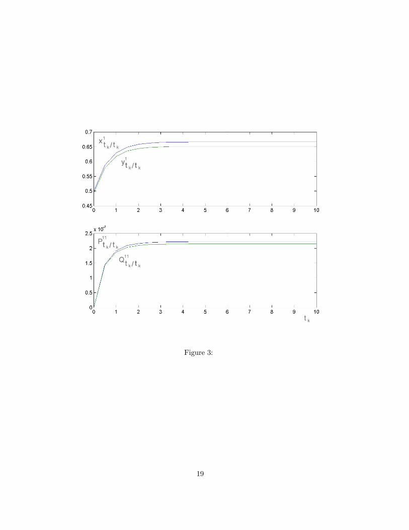
Figure 3:

19

Figure 4:

20

Figure 5:

21

Figure 6:

22

Figure 7:

23

Figure 8:

24

Figure 9:

25

Figure 10:

26