isa-sil

Safety InstrumentedFunctions (SIF) -- SafetyIntegrity Level (SIL)Evaluation TechniquesPart 1: Introduction

Approved 17 June 2002

ISA-TR84.00.02-2002 - Part 1

T E C H N I C A L R E P O R T

ISA The Instrumentation,Systems, and

Automation Society

–TM

ISA-TR84.00.02-2002 – Part 1Safety Instrumented Functions (SIF) Safety Integrity Level (SIL) Evaluation Techniques Part 1:Introduction

ISBN: 1-55617-802-6

Copyright © 2002 by ISA —The Instrumentation, Systems, and Automation Society. All rights reserved.Not for resale. Printed in the United States of America. No part of this publication may be reproduced,stored in a retrieval system, or transmitted in any form or by any means (electronic mechanical,photocopying, recording, or otherwise), without the prior written permission of the Publisher.

ISA67 Alexander DriveP.O. Box 12277Research Triangle Park, North Carolina 27709

− 3 − ISA-TR84.00.02-2002 - Part 1

Preface

This preface, as well as all footnotes and annexes, is included for information purposes and is not part ofISA-TR84.00.02-2002 – Part 1.

This document has been prepared as part of the service of ISAthe Instrumentation, Systems, andAutomation Societytoward a goal of uniformity in the field of instrumentation. To be of real value, thisdocument should not be static but should be subject to periodic review. Toward this end, the Societywelcomes all comments and criticisms and asks that they be addressed to the Secretary, Standards andPractices Board; ISA; 67 Alexander Drive; P. O. Box 12277; Research Triangle Park, NC 27709;Telephone (919) 549-8411; Fax (919) 549-8288; E-mail: [email protected].

The ISA Standards and Practices Department is aware of the growing need for attention to the metricsystem of units in general, and the International System of Units (SI) in particular, in the preparation ofinstrumentation standards. The Department is further aware of the benefits to USA users of ISAstandards of incorporating suitable references to the SI (and the metric system) in their business andprofessional dealings with other countries. Toward this end, this Department will endeavor to introduceSI-acceptable metric units in all new and revised standards, recommended practices, and technicalreports to the greatest extent possible. Standard for Use of the International System of Units (SI): TheModern Metric System, published by the American Society for Testing & Materials as IEEE/ASTM SI 10-97, and future revisions, will be the reference guide for definitions, symbols, abbreviations, andconversion factors.

It is the policy of ISA to encourage and welcome the participation of all concerned individuals andinterests in the development of ISA standards, recommended practices, and technical reports.Participation in the ISA standards-making process by an individual in no way constitutes endorsement bythe employer of that individual, of ISA, or of any of the standards, recommended practices, and technicalreports that ISA develops.

CAUTION — ISA ADHERES TO THE POLICY OF THE AMERICAN NATIONAL STANDARDSINSTITUTE WITH REGARD TO PATENTS. IF ISA IS INFORMED OF AN EXISTING PATENT THAT ISREQUIRED FOR USE OF THE STANDARD, IT WILL REQUIRE THE OWNER OF THE PATENT TOEITHER GRANT A ROYALTY-FREE LICENSE FOR USE OF THE PATENT BY USERS COMPLYINGWITH THE STANDARD OR A LICENSE ON REASONABLE TERMS AND CONDITIONS THAT AREFREE FROM UNFAIR DISCRIMINATION.

EVEN IF ISA IS UNAWARE OF ANY PATENT COVERING THIS STANDARD, THE USER ISCAUTIONED THAT IMPLEMENTATION OF THE STANDARD MAY REQUIRE USE OF TECHNIQUES,PROCESSES, OR MATERIALS COVERED BY PATENT RIGHTS. ISA TAKES NO POSITION ON THEEXISTENCE OR VALIDITY OF ANY PATENT RIGHTS THAT MAY BE INVOLVED IN IMPLEMENTINGTHE STANDARD. ISA IS NOT RESPONSIBLE FOR IDENTIFYING ALL PATENTS THAT MAYREQUIRE A LICENSE BEFORE IMPLEMENTATION OF THE STANDARD OR FOR INVESTIGATINGTHE VALIDITY OR SCOPE OF ANY PATENTS BROUGHT TO ITS ATTENTION. THE USER SHOULDCAREFULLY INVESTIGATE RELEVANT PATENTS BEFORE USING THE STANDARD FOR THEUSER’S INTENDED APPLICATION.

HOWEVER, ISA ASKS THAT ANYONE REVIEWING THIS STANDARD WHO IS AWARE OF ANYPATENTS THAT MAY IMPACT IMPLEMENTATION OF THE STANDARD NOTIFY THE ISASTANDARDS AND PRACTICES DEPARTMENT OF THE PATENT AND ITS OWNER.

ADDITIONALLY, THE USE OF THIS STANDARD MAY INVOLVE HAZARDOUS MATERIALS,OPERATIONS OR EQUIPMENT. THE STANDARD CANNOT ANTICIPATE ALL POSSIBLEAPPLICATIONS OR ADDRESS ALL POSSIBLE SAFETY ISSUES ASSOCIATED WITH USE INHAZARDOUS CONDITIONS. THE USER OF THIS STANDARD MUST EXERCISE SOUND

ISA-TR84.00.02-2002 - Part 1 − 4 −

PROFESSIONAL JUDGMENT CONCERNING ITS USE AND APPLICABILITY UNDER THE USER’SPARTICULAR CIRCUMSTANCES. THE USER MUST ALSO CONSIDER THE APPLICABILITY OFANY GOVERNMENTAL REGULATORY LIMITATIONS AND ESTABLISHED SAFETY AND HEALTHPRACTICES BEFORE IMPLEMENTING THIS STANDARD.

THE USER OF THIS DOCUMENT SHOULD BE AWARE THAT THIS DOCUMENT MAY BE IMPACTEDBY ELECTRONIC SECURITY ISSUES. THE COMMITTEE HAS NOT YET ADDRESSED THEPOTENTIAL ISSUES IN THIS VERSION.

The following people served as members of ISA Committee SP84:

NAME COMPANY

V. Maggioli, Chair Feltronics CorporationR. Webb, Managing Director POWER EngineersC. Ackerman Air Products & Chemicals Inc.R. Adamski InvensysC. Adler Moore Industries International Inc.R. Bailliet Syscon International Inc.N. Battikha Bergo Tech Inc.L. Beckman HIMA Americas Inc.S. Bender S K Bender & AssociatesK. Bond Shell Global SolutionsA. Brombacher Eindhoven University of TechnologyS. Brown* DuPont CompanyJ. Carew ConsultantK. Dejmek Baker Engineering & Lisk ConsultingA. Dowell* Rohm & Haas CompanyR. Dunn* DuPont EngineeringP. Early ABB Industrial Systems Inc.T. Fisher DeceasedJ. Flynt ConsultantA. Frederickson Triconex CorporationR. Freeman ABS ConsultingD. Fritsch Fritsch Consulting ServiceK. Gandhi Kellogg Brown & RootR. Gardner* DupontJ. Gilman ConsultantW. Goble exida.com LLCD. Green* Rohm & Haas CompanyP. Gruhn SiemensC. Hardin CDH Consulting Inc.J. Harris UOP LLCD. Haysley Albert Garaody & AssociatesM. Houtermans TUV Product Service Inc.J. Jamison Bantrel Inc.W. Johnson* E I du PontD. Karydas* Factory Mutual Research CorporationL. Laskowski Solutia Inc.T. Layer Emerson Process ManagementD. Leonard D J Leonard ConsultantsE. Lewis ConsultantE. Marszal Exida.comN. McLeod AtofinaW. Mostia WLM Engineering CompanyD. Ogwude Creative Systems International

− 5 − ISA-TR84.00.02-2002 - Part 1

G. Ramachandran Cytec Industries Inc.K. Schilowsky Marathon Ashland Petroleum Company LLCD. Sniezek Lockheed Martin Federal ServicesC. Sossman WG-W Safety Management SolutionsR. Spiker Yokogawa Industrial Safety Systems BVP. Stavrianidis* Factory Mutual Research CorporationH. Storey Equilon Enterprises LLCA. Summers SIS-TECH Solutions LLCL. Suttinger Westinghouse Savannah River CompanyR. Szanyi ExxonMobil Research EngineeringR. Taubert BASF CorporationH. Tausch Honeywell Inc.T. Walczak GE FANUC AutomationM. Weber System Safety Inc.D. Zetterberg Chevron Texaco ERTC______ * One vote per company.

This standard was approved for publication by the ISA Standards and Practices Board on 17 June 2002.

NAME COMPANY

M. Zielinski Emerson Process ManagementD. Bishop David N Bishop, ConsultantD. Bouchard PapricanM. Cohen ConsultantM. Coppler Ametek, Inc.B. Dumortier Schneider ElectricW. Holland Southern CompanyE. Icayan ACES IncA. Iverson Ivy OptiksR. Jones Dow Chemical CompanyV. Maggioli Feltronics CorporationT. McAvinew ForeRunner CorporationA. McCauley, Jr. Chagrin Valley Controls, Inc.G. McFarland Westinghouse Process Control Inc.R. Reimer Rockwell AutomationJ. Rennie Factory Mutual Research CorporationH. Sasajima Yamatake CorporationI. Verhappen Syncrude Canada Ltd.R. Webb POWER EngineersW. Weidman Parsons Energy & Chemicals GroupJ. Weiss KEMA ConsultingM. Widmeyer Stanford Linear Accelerator CenterC. Williams Eastman Kodak CompanyG. Wood Graeme Wood Consulting

This page intentionally left blank.

− 7 − ISA-TR84.00.02-2002 - Part 1

Contents

Foreword ....................................................................................................................................................... 9

Introduction ................................................................................................................................................. 11

1 Scope................................................................................................................................................... 17

2 References .......................................................................................................................................... 17

3 Definitions of terms and symbols......................................................................................................... 19

3.1 Definition of terms......................................................................................................................... 19

3.2 Definition of symbols .................................................................................................................... 33

4 Probability of failure on demand (PFD) ............................................................................................... 43

5 Modeling of SIF element failures ......................................................................................................... 44

5.1 Physical failures............................................................................................................................ 44

5.2 Hardware common cause failures................................................................................................ 44

5.3 Systematic failures ....................................................................................................................... 44

5.4 Partitioning of SIF element failures .............................................................................................. 46

5.5 Modeling of field devices .............................................................................................................. 49

5.6 Modeling of elements in PES arithmetic/logic solvers.................................................................. 50

5.7 System modeling .......................................................................................................................... 54

5.8 Failure rate data for commonly used field instrumentation .......................................................... 54

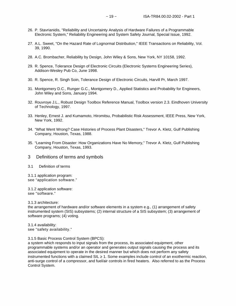
5.9 Statistical data analysis methods ................................................................................................. 57

6 Comparison of system analysis techniques ........................................................................................ 62

Annex A (informative) Methodology for quantifying the effect of hardware-related common causefailures in Safety Instrumented Functions................................................................................................... 67

Annex B (informative) Fault simulation test procedure .......................................................................... 79

Annex C (informative) SIL quantification of SIS – Advisory software packages.................................... 83

Annex D (informative) Failure mode effect, hazard and criticality analysis ........................................... 85

Annex E (informative) Common cause failures and systematic failure checklist................................... 91

Annex F — Index ........................................................................................................................................ 93

− 9 − ISA-TR84.00.02-2002 - Part 1

Safety Instrumented Systems (SIS)

Safety Integrity Level (SIL) Evaluation Techniques

Part 1: Introduction

Foreword

The information contained in ISA-TR84.00.02-2002 is provided for information only and is not part of theANSI/ISA-84.01-1996 Standard (1) requirements.

The purpose of ISA-TR84.00.02-2002 (2) is to provide the process industry with a description of variousmethodologies that can be used to evaluate the Safety Integrity Level (SIL) of Safety InstrumentedFunctions (SIF).

ANSI/ISA-84.01-1996 provides the minimum requirements for implementing a SIS given that a set offunctional requirements have been defined and a SIL requirement has been established for each safetyinstrumented function. Additional information of an informative nature is provided in the Annexes toANSI/ISA-84.01-1996 to assist the designer in applying the concepts necessary to achieve an acceptabledesign. However, Standards Project 84 (SP84) determined that it was appropriate to providesupplemental information that would assist the user in evaluating the capability of any given SIF design toachieve its required SIL. A secondary purpose of this document is to reinforce the concept of theperformance based evaluation of SIF. The performance parameters that satisfactorily service the processindustry are derived from the SIL and reliability evaluation of SIF, namely the probability of the SIF to failto respond to a demand and the probability that the SIF creates a nuisance trip. Such evaluationaddresses the design elements (hardware, software, redundancy, etc.) and the operational attributes(inspection/maintenance policy, frequency and quality of testing, etc.) of the SIF. The basis for theperformance evaluation of the SIF is safety targets determined through hazard analysis and riskassessment (6) of the process. This document demonstrates methodologies for the SIL and reliabilityevaluation of SIF.

The document focuses on methodologies that can be used without promoting a single methodology. Itprovides information on the benefits of various methodologies as well as some of the drawbacks they mayhave.

THE METHODOLOGIES ARE DEMONSTRATED THROUGH EXAMPLES (SISARCHITECTURES) THAT REPRESENT POSSIBLE SYSTEM CONFIGURATIONSAND SHOULD NOT BE INTERPRETED AS RECOMMENDATIONS FOR SIS. THEUSER IS CAUTIONED TO CLEARLY UNDERSTAND THE ASSUMPTIONS AND DATAASSOCIATED WITH THE METHODOLOGIES IN THIS DOCUMENT BEFOREATTEMPTING TO UTILIZE THE METHODS PRESENTED HEREIN.

The users of ISA-TR84.00.02-2002 include:

• Process Hazards Analysis teams that wish to develop understanding of different methodologies indetermining SIL

• SIS designers who want a better understanding of how redundancy, diagnostic coverage, diversity,etc., fit into the development of a proper SIS architecture

• Logic solver and field device suppliers

ISA-TR84.00.02-2002 - Part 1 − 10 −

• National and International standard bodies providing guidance in the use of reliability techniques forSIS architectures

• Reliability engineers (or any engineer performing this function) can use this information to developbetter methods for determining SIL in the rapidly changing SIS field

• Parties who do not have a large installed base of operating equipment sufficient to establishappropriate statistical analysis for PFDavg and MTTFspurious for SIS components

• Operations and maintenance personnel

ISA-TR84.00.02-2002 consists of the following parts, under the general title “Safety InstrumentedFunctions (SIF) Safety Integrity Level (SIL) Evaluation Techniques."

Part 1: Introduction

Part 2: Determining the SIL of a SIF via Simplified Equations

Part 3: Determining the SIL of a SIF via Fault Tree Analysis

Part 4: Determining the SIL of a SIF via Markov Analysis

Part 5: Determining the PFD of Logic Solvers via Markov Analysis

− 11 − ISA-TR84.00.02-2002 - Part 1

Introduction

ANSI/ISA-84.01-1996 describes a safety lifecycle model for the implementation of risk reductionmeasures for the process industry (Clause 4). The standard then proceeds to provide specific guidance inthe application of SIS, which may be one of the risk reduction methods used. The standard defines threelevels of safety integrity (Safety Integrity Levels, SIL) that may be used to specify the capability that asafety instrumented function must achieve to accomplish the required risk reduction. ISA-TR84.00.02-2002 provides methodologies for evaluating SIF to determine if they achieve the specific SIL. This may bereferred to as a probability of failure on demand (PFD) evaluation of the SIF.

ISA-TR84.00.02-2002 only addresses SIF operating in demand mode.

The evaluation approaches outlined in this document are performance-based approaches and do notprovide specific results that can be used to select a specific architectural configuration for a given SIL.

THE READER IS CAUTIONED TO CLEARLY UNDERSTAND THE ASSUMPTIONS ASSOCIATEDWITH THE METHODOLOGY AND EXAMPLES IN THIS DOCUMENT BEFORE DERIVING ANYCONCLUSIONS REGARDING THE EVALUATION OF ANY SPECIFIC SIF.

The evaluation processes described in this document take place before the SIS detailed design phase ofthe life cycle (see Figure I.1, Safety Lifecycle Model).

This document assumes that a SIS is required. It does not provide guidance in the determination of theneed for a SIS. The user is referred to ANSI/ISA-84.01-1996 Annex A for methodologies that might beused in making this determination.

This document involves the evaluation of the whole SIF from the sensors through the logic solverto the final elements. Process industry experience shows that sensors and final elements aremajor contributors to loss of SIS integrity (high PFD). When evaluating the performance ofsensors and final elements, issues such as component technology, installation, and maintenanceshould be considered.

Frequently multiple safety instrumented functions are included in a single logic solver. The logic solvershould be carefully evaluated since a problem in the logic solver may adversely impact the performanceof all of the safety instrumented functions (i.e., the logic solver could be the common cause failure thatdisables all of the SIFs.).

This principle (i.e., common cause) applies to any

• element of a SIS that is common to more than one safety instrumented function; and

• redundant element with one or more safety instrumented function.

Each element should be evaluated with respect to all the safety instrumented functions with which it isassociated

• to ensure that it meets the integrity level required for each safety instrumented function;

• to understand the interactions of all the safety instrumented functions; and

• to understand the impact of failure of each component.

This document does not provide guidance in the determination of the specific SIL required (e.g., SIL 1, 2,and 3) for the SIS. The user is again referred to ANSI/ISA-84.01-1996 or to other references.

ISA-TR84.00.02-2002 - Part 1 − 12 −

The primary focus of this document is on evaluation methodologies for assessing the capability of theSIS. The SIS lifecycle model is defined in ANSI/ISA-84.01-1996. Figure I.2 shows the boundaries of theSIS and how it relates to other systems.

Start

ConceptualProcessDesign

PerformProcess HazardAnalysis & Risk

Assessment

Apply non-SISprotection layers

to preventidentified hazards

or reduce risk

SIS required?

Define Target SILfor each SafetyInstrumented

Function

Develop *Safety

RequirementsSpecification

Perform SIS *Conceptual

Design, & verifyit meets the SRS

Perform SISDetail Design

SIS Installation,Commissioningand Pre-StartupAcceptence Test

EstablishOperation &MaintenanceProcedures

Pre-StartupSafety Review(Assessment)

SIS startup,operation,

maintenance,periodic

functional testing

Modify orDecommission

SIS?

SISDecommissioning

Safety Life Cyclesteps not covered

by 84.01

Safety Life Cyclesteps covered

by 84.01

Safety Life Cycle *steps whereTR84.00.02is applicable

Legend:

No

Yes

Modify

Decommision

Figure I.1 Safety lifecycle model

− 13 − ISA-TR84.00.02-2002 - Part 1

SIS User Interface

Basic Process Control System

SensorsFinalElements

Logic

LogicSolver

Figure I.2 Definition of Safety Instrumented System (SIS)

The safety requirements specification addresses the design elements (hardware, software, redundancy,etc.) and the operational attributes (inspection/maintenance policy, frequency and quality of testing, etc.)of the SIS. These elements affect the PFD of each safety instrumented function.

The PFD of these systems can be determined using historical system performance data (e.g., statisticalanalysis). Where systems, subsystems, components, etc. have not been in use for a sufficiently long timeand in large enough numbers to have a statistically significant population available for the evaluation oftheir performance solely based on actuarial data, a systematic evaluation of the performance of a systemmay be obtained through the use of PFD analysis techniques.

PFD analysis techniques employ systematic methodologies that decompose a complex system to itsbasic components. The performance and interactions of these basic components are merged intoreliability models (such as simplified equations, fault trees, Markov models) to determine the overallsystem safety availability.

This document provides users with a number of PFD evaluation techniques that allow a user to determineif a SIF meets the required safety integrity level.

Safety integrity is defined as “The probability of a Safety Instrumented Function satisfactorily performingthe required safety functions under all stated conditions within a stated period of time.” Safety integrityconsists of two elements: 1) hardware safety integrity and 2) systematic safety integrity. Hardware safetyintegrity which is based upon random hardware failures can normally be estimated to a reasonable levelof accuracy. ANSI/ISA-84.01-1996 addresses the hardware safety integrity by specifying target failuremeasures for each SIL. For SIF operating in the demand mode the target failure measure is PFDavg

(average probability of failure to perform its design function on demand). PFDavg is also commonlyreferred to as the average probability of failure on demand. Systematic integrity is difficult to quantify dueto the diversity of causes of failures; systematic failures may be introduced during the specification,design, implementation, operational and modification phase and may affect hardware as well as software.ANSI/ISA-84.01-1996 addresses systematic safety integrity by specifying procedures, techniques,measures, etc. that reduce systematic failures.

SIS Boundary

ISA-TR84.00.02-2002 - Part 1 − 14 −

An acceptable safe failure rate is also normally specified for a SIF. The safe failure rate is commonlyreferred to as the false trip, nuisance trip, or spurious trip rate. The spurious trip rate is included in theevaluation of a SIF, since process start up and shutdown are frequently periods where chances of ahazardous event are high. Hence in many cases, the reduction of spurious trips will increase the safety ofthe process. The acceptable safe failure rate is typically expressed as the mean time to a spurious trip(MTTFspurious).

NOTE In addition to the safety issue(s) associated with spurious trips the user of the SIS may also want the acceptableMTTFspurious to be increased to reduce the effect of spurious trips on the productivity of the process under control. This increase inthe acceptable MTTFspurious can usually be justified because of the high cost associated with a spurious trip.

The objective of this technical report is to provide users with techniques for the evaluation of the hardwaresafety integrity of SIF (PFDavg) and the determination of MTTFspurious. Methods of modeling systematicfailures are also presented so a quantitative analysis can be performed if the systematic failure rates areknown.

ISA-TR84.00.02-2002 shows how to model complete SIF, which includes the sensors, the logic solverand final elements. To the extent possible the system analysis techniques allow these elements to beindependently analyzed. This allows the safety system designer to select the proper system configurationto achieve the required safety integrity level.

ISA-TR84.00.02-2002 - Part 1 provides

• a detailed listing of the definition of all terms used in this document. These are consistent with theANSI/ISA-84.01-1996, IEC 61508 and IEC 61511 standards.

• the background information on how to model all the elements or components of a SIF. It focuses onthe hardware components, provides some component failure rate data that are used in the examplescalculations and discusses other important parameters such as common cause failures and functionalfailures.

• a brief introduction to the methodologies that will be used in the examples shown in this document.They are Simplified equations (3), Fault Tree Analysis (4), and Markov Analysis (5).

ISA-TR84.00.02-2002 - Part 2 provides simplified equations for calculating the SIL values for DemandMode Safety Instrumented Functions (SIF) installed in accordance with ANSI/ISA-84.01-1996,“Applications of Safety Instrumented Systems for the Process Industries." Part 2 should not beinterpreted as the only evaluation technique that might be used. It does, however, provide theengineer(s) performing design for a SIS with an overall technique for assessing the capability of thedesigned SIF.

ISA-TR84.00.02-2002 - Part 3 provides fault tree analysis techniques for calculating the SIL for DemandMode Safety Instrumented Functions (SIF) installed in accordance with ANSI/ISA-84.01-1996,“Applications of Safety Instrumented Systems for the Process Industries." Part 3 should not beinterpreted as the only evaluation technique that might be used. It does, however, provide theengineer(s) performing design for a SIS with an overall technique for assessing the capability of thedesigned SIF.

ISA-TR84.00.02-2002 - Part 4 provides Markov analysis techniques for calculating the SIL values forDemand Mode Safety Instrumented Functions (SIF) installed in accordance with ANSI/ISA-84.01-1996,“Applications of Safety Instrumented Systems for the Process Industries." Part 4 should not beinterpreted as the only evaluation technique that might be used. It does, however, provide theengineer(s) performing design for a SIS with an overall technique for assessing the capability of thedesigned SIF.

− 15 − ISA-TR84.00.02-2002 - Part 1

ISA-TR84.00.02-2002 - Part 5 addresses the logic solver only, using Markov Models for calculating thePFD of E/E/PE logic solvers because it allows the modeling of maintenance and repairs as a function oftime, treats time as a model parameter, explicitly allows the treatment of diagnostic coverage, and modelsthe systematic failures (i.e., operator failures, software failures, etc.) and common cause failures.

Figure I.3 illustrates the relationship of each part to all other parts.

ISA-TR84.00.02-2002 - Part 1 − 16 −

Figure I.3 ISA-TR84.00.02-2002 Overall Framework

Part 1

Part 2

Part 3

Part 4

Part 5

Development of the overall terms, symbols, explanation of

SIS element failures, comparison of system analysis

techniques, and uncertainty analysis examples.

Development of SIL for SIF using

Simplified Equation Methodology.


Fault Tree Analysis Methodology.


Markov Analysis Methodology.

Guidance in

determining

the PFD of

E/E/PE logic

solver(s) via

Markov

Analysis.

− 17 − ISA-TR84.00.02-2002 - Part 1

1 Scope

1.1 ISA-TR84.00.02-2002 - Part 1 is informative and does not contain any mandatory clauses. ISA-TR84.00.02-2002 is intended to be used only with a thorough understanding of ANSI/ISA-84.01-1996(see Figure I.1). Prior to proceeding with use of ISA-TR84.00.02-2002 in a safety application, theHazards and Risk Analysis must have been completed and the following information provided

a) It is determined that a SIS is required.

b) Each safety instrumented function to be carried out by the SIS(s) is defined.

c) The SIL for each safety instrumented function is defined.

1.2 ISA-TR84.00.02-2002 - Part 1 provides

a) guidance in Safety Integrity Level analysis;

b) methods to implement Safety Instrumented Functions (SIF) to achieve a specified SIL;

c) discussion of failure rates and failure modes (Annex D) of SIS and their components;

d) discussion of diagnostic coverage, covert faults, common cause, systematic failures, redundancy ofSIF;

e) tool(s) for verification of SIL; and

f) discussion of the effect of functional test interval.

1.3 The objective of ISA-TR84.00.02-2002 - Part 1 is to introduce the reader to the performance basedapproach for evaluating the reliability of SIF and to present system reliability methodologies that can beused to evaluate the system performance parameters, namely, the probability that the SIF fails to respondto a demand and the probability that the SIF creates a nuisance trip. ISA-TR84.00.02-2002 - Part 1serves as an introduction for all other parts.

2 References

1. ANSI/ISA-84.01-1996 “Application of Safety Instrumented Systems for the Process Industries," ISA,Research Triangle Park, NC, 27709, February 1996.

2. ISA-TR84.00.02-2002, "Safety Instrumented Functions (SIF) – Safety Integrity Level EvaluationTechniques, Part 1: Introduction; Part 2: Determining the SIL of a SIF via Simplified Equations; Part 3:Determining the SIL of a SIF via Fault Tree Analysis; Part 4: Determining the SIL of a SIF via MarkovAnalysis; Part 5: Determining the PFDavg of SIS Logic Solvers via Markov Analysis,"Instrumentation, Systems and Automation Society, Technical Report, Research Triangle Park, NC,27709, 2002.

3. Reliability, Maintainability and Risk (Practical Methods for Engineers), 4th Edition, D.J. Smith,Butterworth-Heinemann, 1993, ISBN 0-7506-0854-4.

4. “Guidelines for Safe Automation of Chemical Processes," Center for Chemical Process Safety,American Institute of Chemical Engineers, New York, NY 10017, 1993

5. “Evaluating Control Systems Reliability”, W. M. Goble, Instrument Society of America, ResearchTriangle Park, NC, 27709, 1992.

ISA-TR84.00.02-2002 - Part 1 − 18 −

6. “Introduction to Reliability Engineering," E.E. Lewis, John Wiley & Sons, New York, NY 10158, 1987.

7. “Assurance Technologies - Principles and Practices," D.G. Raheja, McGraw and Hill Inc., New York,NY, 1991.

8. “Safeware - System Safety and Computers," N.G. Levenson, Addison-Wesley Publishing Co.,Reading, MA, 1995.

9. “Reliability by Design," A.C. Brombacher, John Wiley & Sons, New York, NY 10158, 1992.

10. “Software Reliability Handbook," P. Rook, Elsevier Science Press, New York, NY 10010, 1990.

11. “Guidelines for Chemical Process Quantitative Risk Analysis, Center for Chemical Process Safety,New York, NY, American Institute of Chemical Engineers, 1989.

12. “The 'Why’s' of Grounding Isolated Ground Planes and Power Supplies, ISBN 0-941247-00-7,Licensing Division, Bell Communications Research, Inc., 290 W. Mt. Pleasant Ave., Livingston, NJ07039-2729, 1989.

13. “Reliability Evaluation of Engineering Systems," R. Billinton, R.N. Allan, Pitman Advanced PublishingProgram, Marshfield, MA 02050, 1983.

14. OREDA-92 (Offshore Reliability Data) DNV Industry, 1992, ISBN 82-515-0188-1.

15. Guidelines For Process Equipment Reliability Data With Data Tables, American Institute of ChemicalEngineers, Center for Chemical Process Safety, 1989, ISBN 8169-0422-7.

16. IEEE Std 500-1984, Equipment Reliability Data for Nuclear Power Generating Stations, IEEE andJohn Wiley & Sons, 1974, ISBN 471-80785-0.

17. RAC, Reliability Analysis Centre-1991, NSN7540-01-280-5500.

18. MIL-Handbook-217, Reliability Prediction of Electronic Equipment.

19. Programmable electronic systems in safety-related applications, Part 2: General technical guidelines,Health and Safety Executive, HMSO, ISBN 0 11 883906 3, 1987.

20. Assigning a numerical value to the beta factor common cause evaluation, Humphreys, R. A.,Reliability '87.

21. UPM3.1: A pragmatic approach to dependent failures assessment for standard systems, AEATechnology, ISBN 085 356 4337.

22. G. Apostolakis, S. Kaplan, "Methodology for Probabilistic Risk Assessment of Nuclear Power Plants,"Technical Report, Pickard, Lowe and Garrick Inc., 1981.

23. G. Apostolakis, J.S. Wu and D. OKrent, "Uncertainties in System Reliability: Probabilistic versusNonprobabilistic Theories," Reliability Engineering and System Safety, Vol. 30, 1991.

24. M. Evans, N. Hastings and B. Peacock, “Statistical Distributions," 2nd edition, John Wiley & Sons, NY,1993.

25. G. Fishman, "Concepts and Methods in Discrete Event Simulation," John Wiley & Sons, NY, 1983.

− 19 − ISA-TR84.00.02-2002 - Part 1

26. P. Stavrianidis, "Reliability and Uncertainty Analysis of Hardware Failures of a ProgrammableElectronic System," Reliability Engineering and System Safety Journal, Special Issue, 1992.

27. A.L. Sweet, "On the Hazard Rate of Lognormal Distribution," IEEE Transactions on Reliability, Vol.39, 1990.

28. A.C. Brombacher, Reliability by Design, John Wiley & Sons, New York, NY 10158, 1992.

29. R. Spence, Tolerance Design of Electronic Circuits (Electronic Systems Engineering Series),Addison-Wesley Pub Co, June 1998.

30. R. Spence, R. Singh Soin, Tolerance Design of Electronic Circuits, Harvill Pr, March 1997.

31. Montgomery D.C., Runger G.C., Montgomery D., Applied Statistics and Probability for Engineers,John Wiley and Sons, January 1994.

32. Rouvroye J.L., Robust Design Toolbox Reference Manual, Toolbox version 2.3. Eindhoven Universityof Technology, 1997.

33. Henley, Ernest J. and Kumamoto, Hiromitsu, Probabilistic Risk Assessment, IEEE Press, New York,New York, 1992.

34. “What Went Wrong? Case Histories of Process Plant Disasters," Trevor A. Kletz, Gulf PublishingCompany, Houston, Texas, 1988.

35. “Learning From Disaster: How Organizations Have No Memory," Trevor A. Kletz, Gulf PublishingCompany, Houston, Texas, 1993.

3 Definitions of terms and symbols

3.1 Definition of terms

3.1.1 application program:see “application software.”

3.1.2 application software:see “software.”

3.1.3 architecture:the arrangement of hardware and/or software elements in a system e.g., (1) arrangement of safetyinstrumented system (SIS) subsystems; (2) internal structure of a SIS subsystem; (3) arrangement ofsoftware programs; (4) voting.

3.1.4 availability:see “safety availability.”

3.1.5 Basic Process Control System (BPCS):a system which responds to input signals from the process, its associated equipment, otherprogrammable systems and/or an operator and generates output signals causing the process and itsassociated equipment to operate in the desired manner but which does not perform any safetyinstrumented functions with a claimed SIL ≥ 1. Some examples include control of an exothermic reaction,anti-surge control of a compressor, and fuel/air controls in fired heaters. Also referred to as the ProcessControl System.

ISA-TR84.00.02-2002 - Part 1 − 20 −

3.1.6 channel:a channel is an element or a group of elements that independently perform(s) a function. The elementswithin a channel could include input/output(I/O) modules, logic system, sensors, and final elements. Theterm can be used to describe a complete system, or a portion of a system (for example, sensors or finalelements).

NOTE A dual channel (i.e., a two channel) configuration is one with two channels that independently perform the same function.

3.1.7 common cause:

3.1.7.1. common cause fault:a single fault that will cause failure in two or more channels of a multiple channel system. The singlesource may be either internal or external to the system.

3.1.7.2 common cause failure: a failure, which is the result of one or more events causing coincident failures of two or more separatechannels in a multiple channel system, leading to a system failure.

3.1.8 communication:

3.1.8.1 external communication:data exchange between the SIS and a variety of systems or devices that are outside the SIS.These include shared operator interfaces, maintenance/engineering interfaces, data acquisitionsystems, host computers, etc.

3.1.8.2 internal communication:data exchange between the various devices within a given SIS. These include bus backplaneconnections, the local or remote I/O bus, etc.

3.1.9 coverage:see “diagnostic coverage.”

3.1.10 overt:see "undetected."

3.1.11 Cumulative Distribution Function (CDF):the integral, from zero to infinity, of the failure rate distribution and takes values between zero and one.

3.1.12 dangerous failure:a failure which has the potential to put the safety instrumented function in a hazardous or fail-to-functionstate.

NOTE Whether or not the potential is realised may depend on the channel architecture of the system; in systems with multiplechannels to improve safety, a dangerous hardware failure is less likely to lead to the overall hazardous or fail-to-function state.

3.1.13 decommissioning:the permanent removal of a complete SIS from active service.

3.1.14 de-energize to trip:SIS circuits where the outputs and devices are energized under normal operation. Removal of the sourceof power (e.g., electricity, air) causes a trip action.

− 21 − ISA-TR84.00.02-2002 - Part 1

3.1.15 demand:a condition or event that requires the SIS to take appropriate action to prevent a hazardous event fromoccurring or to mitigate the consequence of a hazardous event.

3.1.16 detected:in relation to hardware and software, detected by the diagnostic tests, or through normal operation.

NOTE 1 For example, physical inspection and manual tests, or through normal operation.

NOTE 2 These adjectives are used in detected fault and detected failure.

NOTE 3 Synonyms include: revealed and overt.

3.1.17 diagnostic coverage: the diagnostic coverage of a component or subsystem is the ratio of the detected failure rates to the totalfailure rates of the component or subsystem as detected by automatic diagnostic tests.

NOTE 1 Diagnostic coverage factor is synonymous with diagnostic coverage.

NOTE 2 The diagnostic coverage is used to compute the detected (λD) and undetected failure rates (λU) from the total failure rate(λT) as follows: λD = DC x λT and λU = (1-DC) x λT

NOTE 3 Diagnostic coverage is applied to components or subsystems of a safety instrumented system. For example thediagnostic coverage is typically determined for a sensor, final element, or a logic solver.

NOTE 4 For safety applications the diagnostic coverage is typically applied to the safe and dangerous failures of a component orsubsystem. For example the diagnostic coverage for the dangerous failures of a component or subsystem is DC = λDD/λDT , whereλDD is the dangerous detected failure rates and λDT is the total dangerous failure rate.

3.1.18 diverse:use of different technologies, equipment or design methods to perform a common function with the intentto minimize common cause faults.

3.1.19 Electrical (E)/ Electronic (E)/ Programmable Electronic Systems (PES) [E/E/PES]:when used in this context, electrical refers to logic functions performed by electromechanical techniques,(e.g., electromechanical relay, motor driven timers, etc.), electronic refers to logic functions performed byelectronic techniques, (e.g., solid state logic, solid state relay, etc.), and programmable electronic systemrefers to logic performed by programmable or configurable devices [e.g., Programmable Logic Controller(PLC), Single Loop Digital Controller (SLDC), etc.]. Field devices are not included in E/E/PES.

3.1.20 Electronic (/E):see “E/E/PES.”

3.1.21 embedded software:see “software.”

3.1.22 energize to trip:SIS circuits where the outputs and devices are de-energized under normal operation. Application ofpower (e.g., electricity, air) causes a trip action.

3.1.23 Equipment Under Control (EUC):equipment, machinery, operations or plant used for manufacturing, process, transportation, medical orother activities. In IEC 61511, the term “process” is used instead of Equipment Under Control to reflectprocess sector usage.

ISA-TR84.00.02-2002 - Part 1 − 22 −

3.1.24 fail-to-danger:the state of a SIF in which the SIF cannot respond to a demand. Fail-to-function is used in this document(see fail-to-function).

3.1.25 fail-to-function:the state of a SIF during which the SIF cannot respond to a demand.

3.1.26 fail-safe:the capability to go to a predetermined safe state in the event of a specific malfunction.

3.1.27 failure:the termination of the ability of a functional unit to perform a required function.

NOTE 1 Performance of required functions necessarily excludes certain behaviour, and some functions may be specified in termsof behaviour to be avoided. The occurrence of such behaviour is a failure.

NOTE 2 Failures are either random or systematic.

3.1.28 failure rate:the average rate at which a component could be expected to fail.

3.1.29 fault:an abnormal condition that may cause a reduction in, or loss of, the capability of a functional unit toperform a required function.

3.1.30 fault tolerance:built-in capability of a system to provide continued correct execution of its assigned function in thepresence of a limited number of hardware and software faults.

3.1.31 field devices:equipment connected to the field side of the SIS logic solver I/O terminals. Such equipment includes fieldwiring, sensors, final control elements and those operator interface devices hard-wired to SIS logic solverI/O terminals.

3.1.32 final element:the part of a safety instrumented system which implements the physical action necessary to achieve asafe state.

NOTE 1 Examples are valves, switch gear, motors including their auxiliary elements e.g., a solenoid valve and actuator if involvedin the safety instrumented function.

NOTE 2 This definition is process sector specific only.

3.1.33 firmware:special purpose memory units containing embedded software in protected memory required for theoperation of programmable electronics.

3.1.34 functional safety:the ability of a safety instrumented system or other means of risk reduction to carry out the actionsnecessary to achieve or to maintain a safe state for the process and its associated equipment.

NOTE 1 This term is not used in ANSI/ISA-84.01-1996. It is used in the IEC 61508 and IEC 61511 standards.

NOTE 2 This definition is from IEC 61511 and it deviates from the definition in IEC 61508-4 to reflect differences in the processsector.

− 23 − ISA-TR84.00.02-2002 - Part 1

3.1.35 functional safety assessment:an investigation, based on evidence, to judge the functional safety achieved by one or more protectionlayers.

NOTE 1 This term is not used in ANSI/ISA-84.01-1996. It is used in the IEC 61508 and IEC 61511 standards.

NOTE 2 This definition is from IEC 61511 and it deviates from the definition in IEC 61508-4 to reflect differences in the processsector.

3.1.36 functional safety audit: a systematic and independent examination to determine whether the procedures specific to the functionalsafety requirements comply with the planned arrangements, are implemented effectively and are suitableto achieve the specified objectives.

NOTE A functional safety audit may be carried out as part of a functional safety assessment.

3.1.37 functional testing:periodic activity to verify that the devices associated with the SIS are operating per the SafetyRequirements Specification. May also be called the proof testing or full function testing.

3.1.38 hardware configuration:see “architecture.”

3.1.39 harm:physical injury or damage to the health of people either directly, or indirectly as a result of damage toproperty or to the environment.

3.1.40 hazard:potential source of harm.

NOTE The term includes danger to persons arising within a short time scale (for example, fire and explosion) and also those thathave a long term effect on a person’s health (for example, release of a toxic substance).

3.1.41 Hazard and Operability Study (HAZOP):a systematic qualitative technique to identify process hazards and potential operating problems using aseries of guide words to study process deviation. A HAZOP is used to examine every part of the processto discover that deviations from the intention of the design can occur and what their causes andconsequences may be. This is done systematically by applying suitable guidewords. This is a systematicdetailed review technique for both batch or continuous plants which can be applied to new or existingprocess to identify hazards.

3.1.42 input function:a function which monitors the process and its associated equipment in order to provide input informationfor the logic solver

NOTE 1 An input function could be a manual function.


3.1.43 input/output modules:

3.1.43.1 input module:E/E/PES or subsystem that acts as the interface to external devices and converts input signals intosignals that the E/E/PES can utilize.

ISA-TR84.00.02-2002 - Part 1 − 24 −

3.1.43.2 output module:E/E/PES or subsystem that acts as the interface to external devices and converts output signals intosignals that can actuate field devices.

3.1.44 logic function:a function which performs the transformations between input information (provided by one or more inputfunctions) and output information (used by one or more output functions). Logic functions provide thetransformation from one or more input functions to one or more output functions.

3.1.45 logic solver:that portion of either a BPCS or SIS that performs one or more logic function(s).

NOTE 1 In ANS/ISA-84.01-1996 and IEC 61511 the following logic systems are used:

� electrical logic systems for electro-mechanical technology;

� electronic logic systems for electronic technology;

� PE logic systems for programmable electronic systems.

NOTE 2 Examples are: electrical systems, electronic systems, programmable electronic systems, pneumatic systems, hydraulicsystems, etc. Sensors and final elements are not part of the logic solver.

NOTE 3 This term deviates from the definition in IEC 61508-4 to reflect differences in the process sector.

3.1.46 mean time to fail - spurious (MTTFspurious):the mean time to a failure of the SIS which results in a spurious or false trip of the process or equipmentunder control (EUC).

3.1.47 mean time to repair (MTTR):the mean time to repair a module or element of the SIS. This mean time is measured from the time thefailure occurs to the time the repair is completed and device returned to service (see MTTROT).

3.1.48 off-line:process, to which the SIS is connected, is shutdown.

3.1.49 on-line:process, to which the SIS is connected, is operating.

3.1.50 output function:function which controls the process and its associated equipment according to final actuator informationfrom the logic function.

NOTE This definition is process sector specific only.

3.1.51 overt:see "detected."

3.1.52 preventive maintenance:maintenance practice in which equipment is maintained on the basis of a fixed schedule, dictated bymanufacturer’s recommendation or by accumulated data from operating experience.

− 25 − ISA-TR84.00.02-2002 - Part 1

3.1.53 Probability of Failure on Demand (PFD):a value that indicates the probability of a system failing to respond to a demand. The average probabilityof a system failing to respond to a demand in a specified time interval is referred to as PFDavg. PFDequals 1 minus Safety Availability. It is also referred to as safety unavailability or fractional dead time.

3.1.54 Probability to Fail Safe (PFS):a value that looks at all failures and indicates the probability of those failures that are in a safe mode.

3.1.55 process Industries:refers to those industries with processes involved in, but not limited to, the production, generation,manufacture, and/or treatment of oil, gas, wood, metals, food, plastics petrochemicals, chemical, steam,electric power, pharmaceuticals and waste material(s). The various process industries together make upthe process sector – a term used in IEC standards.

3.1.56 programmable electronics (PE):electronic component or device forming part of a PES and based on computer technology. The termencompasses both hardware and software and input and output units.

NOTE 1 This term covers micro-electronic devices based on one or more central processing units (CPUs) together withassociated memories, etc. Examples of process sector programmable electronics include:

� smart sensors;

� programmable electronic logic solvers including:

� programmable controllers;

� programmable logic controllers (PLC) (see figure 3.1);

� distributed control system (DCS);

� loop controllers; and

� smart final elements.

NOTE 2 This term differs from the definition in IEC 61508-4 to reflect differences in the process sector.

ISA-TR84.00.02-2002 - Part 1 − 26 −

Figure 3.1 – Structure and function of PLC system (copied from IEC 61131)

Mainssupply

INTERFACE functions tosensors and actuators

DATAstoragefunctions

APPLICATIONPROGRAMstorage functions

OPERATINGSYSTEMfunctions

APPLICATIONPROGRAMExecution

Communicationfunctions

Programming,debugging andtesting functions

MAN –MACHINEINTERFACEfunctions

Other Systems

Machine/Process

Powersupplyfunction

Signalprocessingfunctions

− 27 − ISA-TR84.00.02-2002 - Part 1

3.1.57 programmable electronic system (PES):a system for control, protection or monitoring based on one or more programmable electronic devices,including all elements of the system such as power supplies, sensors and other input devices, datahighways and other communication paths, actuators and other output devices (see Figure 3.2).

NOTE The structure of a PES is shown in Figure 3.2 (A). (B) illustrates the way in which a PES is represented with theprogrammable electronics shown as a unit distinct from sensors and actuators on the process and their interfaces but theprogrammable electronics could exist at several places in the PES. (C) illustrates a PES with two discrete units of programmableelectronics. (D) illustrates a PES with dual programmable electronics (i.e., two channels) but with a single sensor and a singleactuator. (E) illustrates a system based on non-programmable hardware.

(A) Basic PES structure

(B) Single PES with singlePE (i.e., one PES comprisedof a single channel of PE)

(C) Single PES with dualPE linked in a serialmanner (e.g., intelligentsensor and programmablecontroller)

(D) Single PES with dual PEbut with shared sensors andfinal elements (i.e., one PEScomprised of two channelsof PE)

(E) Single non-programmablesystem (e.g., electrical/electronic/pneumatic/hydraulic)

PE PE1 PE2 PE1

PE2

NP

Programmableelectronics (PE)

(see note)

communicationsinput interfacesA-D converters

output interfacesD-A converters

extent ofPES

NOTE: The programmable electronics are shown centrally located but could exist at several places in the PES

input devices(e.g., sensors)

output devices/final elements(e.g., actuators)

Figure 3.2 – Programmable e lectronic system (PES): structure and terminology

3.1.58 proof testing:see “functional testing.”

3.1.59 protection layer:any independent mechanism that reduces risk by control, prevention or mitigation.

NOTE 1 It could be a process engineering mechanism, such as the size of vessels containing hazardous chemicals; a mechanicalengineering mechanism, such as a relief valve; a safety instrumented system; or an administrative procedure, such as anemergency plan against an imminent hazard. These responses may be automated or initiated by human actions.


3.1.60 qualitative methods:methods of design and evaluation developed through experience or the application of good engineeringjudgement.

3.1.61 quantitative methods:methods of design and evaluation based on numerical data and mathematical analysis.

ISA-TR84.00.02-2002 - Part 1 − 28 −

3.1.62 random hardware failure:failure occurring at random time, which results from one or more of the possible degradation mechanismsin the hardware.

NOTE 1 There are many degradation mechanisms occurring at different rates in different components and since manufacturingtolerances cause components to fail due to these mechanisms after different times in operation, failures of a total equipmentcomprising many components occur at predictable rates but at unpredictable (i.e., random) times.

NOTE 2 A major distinguishing feature between random hardware failures and systematic failures (see definition below), is thatsystem failure rates (or other appropriate measures), arising from random hardware failures, can be predicted with reasonable accuracy but systematic failures, by their very nature, cannot be accurately predicted. That is, system failure rates arising fromrandom hardware failures can be quantified with reasonable accuracy but those arising from systematic failures cannot be accurately statistically quantified because the events leading to them cannot easily be predicted.

3.1.63 redundancy:use of multiple elements or systems to perform the same function. Redundancy can be implemented byidentical elements (identical redundancy) or by diverse elements (diverse redundancy).

NOTE 1 Examples are the use of duplicate functional components and the addition of parity bits.

NOTE 2 Redundancy is used primarily to improve reliability or availability.

3.1.64 reliability:probability that a system can perform a defined function under stated conditions for a given period of time.

3.1.65 reliability block diagram:the reliability block diagram can be thought of as a flow diagram from the input of the system to the outputof the system. Each element of the system is a block in the reliability block diagram and, the blocks areplaced in relation to the SIS architecture to indicate that a path from the input to the output is broken ifone (or more) of the elements fail.

3.1.66 risk:the combination of the probability of occurrence of harm and the severity of that harm.

3.1.67 risk assessment:process of making risk estimates and using the results to make decisions.

3.1.68 safe failure:a failure which does not have the potential to put the safety instrumented function in a dangerous or fail-to-function state.

NOTE Other used names for safe failures are: nuisance failure, spurious failure, false trip failure or fail to safe failure.

3.1.69 safe failure fraction (SFF):the fraction of the overall failure rate of a device that results in either a safe failure or a detected unsafefailure.

3.1.70 safety:freedom from unacceptable risk.

3.1.71 safe state:state of the process when safety is achieved.

NOTE 1 In going from a potentially hazardous condition to the final safe state the process may have to go through a number ofintermediate safe-states. For some situations a safe state exists only so long as the process is continuously controlled. Suchcontinuous control may be for a short or an indefinite period of time.

− 29 − ISA-TR84.00.02-2002 - Part 1


3.1.72 safety availability:probability that a SIS is able to perform its designated safety service when the process is operating. Theaverage Probability of Failure on Demand (PFDavg) is the preferred term. (PFD equals 1 minus SafetyAvailability).

3.1.73 safety function:a function to be implemented by a SIS, other technology safety-related system or external risk reductionfacilities, which is intended to achieve or maintain a safe state for the process, in respect of a specifichazardous event.

NOTE This term deviates from the definition in IEC 61508-4 to reflect differences in the process sector.

3.1.74 safety instrumented function (SIF):an E/E/PE safety function with a specified safety integrity level which is necessary to achieve functionalsafety.


3.1.75 safety instrumented system (SIS):implementation of one or more safety instrumented functions. A SIS is composed of any combination ofsensor(s), logic solver(s), and final elements(s) (e.g., see Figure 3.3) Other terms commonly used includeEmergency Shutdown System (ESD, ESS), Safety Shutdown System (SSD), and Safety InterlockSystem.

NOTE SIS may or may not include software.

Figure 3.3 – Example SIS architecture

3.1.76 safety integrity:the probability of a SIF satisfactorily performing the required safety functions under all stated conditionswithin a stated period of time.

NOTE 1 The higher the level of safety integrity of the safety instrumented function (SIF), the lower the probability that the SIFshould fail to carry out the required safety instrumented functions.

NOTE 2 ANSI/ISA-84.01-1996 recognizes three levels of safety integrity for safety instrumented functions. IEC 61508 and IEC61511 recognize four levels of safety integrity.

NOTE 3 In determining safety integrity, all causes of failures (both random hardware failures and systematic failures) which lead toan unsafe state should be included; for example, hardware failures, software induced failures and failures due to electricalinterference. Some of these types of failure, in particular random hardware failures, may be quantified using such measures as thefailure rate in the dangerous mode of failure or the probability of a safety instrumented function failing to operate on demand.

Sensors Logic solver Final elements

PEPE

NP

S/WH/W

SIS architecture andsafety instrumentedfunction example withdifferent devices shown.

PENP

H/W S/W

PENP

H/W S/W

ISA-TR84.00.02-2002 - Part 1 − 30 −

However, the safety integrity of a SIF also depends on many factors, which cannot be accurately quantified but can only beconsidered qualitatively.

NOTE Safety integrity comprises hardware safety integrity and systematic safety integrity.

3.1.77 safety integrity level (SIL):discrete level (one out of four) for specifying the safety integrity requirements of the safety instrumentedfunctions to be allocated to the safety instrumented systems. Safety integrity level 4 has the highest levelof safety integrity; safety integrity level 1 has the lowest.

NOTE 1 ANSI/ISA-84.01-1996 recognizes only three Safety Integrity Levels. The above definition is used in this document toprovide compatibility with IEC 61508 and IEC 61511.

NOTE 2 The target failure measures for the safety integrity levels are specified in Table 3.1.

NOTE 3 It is possible to use several lower safety integrity level systems to satisfy the need for a higher level function (e.g., using aSIL 2 and a SIL 1 system together to satisfy the need for a SIL 3 function). See IEC 61511-2 for guidance on how to apply thisprinciple.

NOTE 4 This term differs from the definition in IEC 61508-4 to reflect differences in the process sector.

Table 3.1 Safety integrity level (SIL) target ranges

Safety Integrity Level

(SIL)

Target Range

Probability of Failure on

Demand Average

(PFDavg)

1 10-1 to 10-2

2 10-2 to 10-3

3 10-3 to 10-4

4 10-4 to 10-5

3.1.78 safety lifecycle:the necessary activities involved in the implementation of safety instrumented function(s), occurringduring a period of time that starts at the concept phase of a project and finishes when all of the safetyinstrumented functions are no longer available for use.

NOTE The term “functional safety lifecycle “ is strictly more accurate, but the adjective “functional” is not considered necessary inthis case within the context of this technical report.

3.1.79 safety requirements specification:the specification that contains all the requirements of the safety instrumented functions that have to beperformed by the safety instrumented systems.

3.1.80 sensor:a device or combination of devices, which measure the process condition (e.g., transmitters, transducers,process switches, position switches, etc.).


− 31 − ISA-TR84.00.02-2002 - Part 1

3.1.81 separation:the use of multiple devices or systems to segregate control from safety instrumented functions.Separation can be implemented by identical elements (identical separation) or by diverse elements(diverse separation).

3.1.82 SIS components:a constituent part of a SIS. Examples of SIS components are field devices, input modules, and logicsolvers.

3.1.83 software:an intellectual creation comprising the programs, procedures, data, rules and any associateddocumentation pertaining to the operation of a data processing system.

NOTE Software is independent of the medium on which it is recorded.

3.1.84 software languages in SIS subsystems:

3.1.84.1 fixed program language (FPL):this type of language is represented by the many proprietary, dedicated-function systems which areavailable as standard process industry products.

The functional specification of the FPL should be documented either in the suppliers’ data sheets, usermanual or the like.

The user should be unable to alter the function of the product, but limited to adjust a few parameters (e.g.,range of the pressure transmitter).

NOTE Typical example of systems with FPL: smart sensor (e.g., pressure transmitter), sequence of events controller, dedicatedsmart alarm box, small data logging systems.

3.1.84.2 limited variability language (LVL):this type of language is a more flexible language which provides the user with some capability foradjusting it to his own specific requirements. The safety instrumented functions are configured by the useof an application-related language and the specialist skills of a computer programmer are not required.

The documentation of the LVL should consist of a comprehensive specification which defines the basicfunctional components and the method of configuring them into an application program. In addition anengineering tool and a library of application specific functions should be given together with a usermanual.

The user should be able to configure/program the required application functions according to thefunctional requirement specification.

NOTE 1 Typical examples of LVL are ladder logic, function block diagram and sequential function chart.

NOTE 2 Typical example of a system using LVL is a standard programmable logic controller (PLC) performing burnermanagement.

3.1.84.3 full variability language (FVL):this type of language is general-purpose computer-based, equipped with an operating system whichusually provides system resource allocation and a real-time multi-programming environment. Thelanguage is tailored for a specific application by computer specialists, using high level languages.

The FVL application will often be unique for a specific application. As a result most of the specification willbe special-to-project.

ISA-TR84.00.02-2002 - Part 1 − 32 −

NOTE 1 Typical example of a system using FVL is a personal computer which performs supervisory control or process modeling.

NOTE 2 In the process sector FVL is found in embedded software and rarely in application software.

NOTE 3 FVL examples include: ADA, C, Pascal.


3.1.85 software program types:

3.1.85.1 application software:software specific to the user application in that it is the SIS functional description programmed in the PESto meet the overall Safety Requirement Specifications. In general, it contains logic sequences,permissives, limits, expressions, etc., that control the appropriate input, output, calculations, decisionsnecessary to meet the safety instrumented functional requirements. See fixed and limited variabilitysoftware language.

3.1.85.2 system software:software that is part of the system supplied by the manufacturer and is not accessible for modification bythe end user. Embedded software is also referred to as firmware or system software.

3.1.85.3 utility software:software tools for the creation, modification, and documentation of application programs. These softwaretools are not required for the operation of the SIS.


3.1.86 software lifecycle:the activities occurring during a period of time that starts when software is conceived and ends when thesoftware is permanently disused.

NOTE 1 A software lifecycle typically includes a requirements phase, development phase, test phase, integration phase,installation phase and modification phase.

NOTE 2 Software cannot be maintained; rather, it is modified.

3.1.87 spurious trip:refers to the shutdown of the process for reasons not associated with a problem in the process that theSIF is designed to protect (e.g., the trip resulted due to a hardware fault, software fault, transient, groundplane interference, etc.). Other terms used include nuisance trip and false shutdown.

3.1.88 Spurious Trip Rate (STR):the expected rate (number of trips per unit time) at which a trip of the SIF can occur for reasons notassociated with a problem in the process that the SIF is designed to protect (e.g., the trip resulted due toa hardware fault, software fault, electrical fault, transient, ground plane interference(12), etc.). Other termsused include nuisance trip rate and false shutdown rate.

3.1.89 systematic failure:failure related in a deterministic way to a certain cause, which can only be eliminated by a modification ofthe design or of the manufacturing process, operational procedures, documentation or other relevantfactors.

NOTE 1 Corrective maintenance without modification should usually not eliminate the failure cause.

NOTE 2 A systematic failure can be induced by simulating the failure cause.

NOTE 3 Example causes of systematic failures include human error in:

− 33 − ISA-TR84.00.02-2002 - Part 1

� the safety requirements specification;

� the design, manufacture, installation and operation of the hardware;

� the design, implementation, etc. of the software.

3.1.90 Test Interval (TI):time between functional tests. Test interval is the amount of time that lapses between functional testsperformed on the SIS or a component of the SIS to validate its operation.

3.1.91 undetected:in relation to hardware and software, not found by the diagnostic tests or during normal operation.

NOTE 1 For example, physical inspection and manual tests, or through normal operation.

NOTE 2 These adjectives are used in undetected fault and undetected failure.

NOTE 3 Synonyms include: unrevealed and covert.


3.1.92 utility software:see “software.”

3.1.93 verification:process of confirming for certain steps of the Safety Life Cycle that the objectives are met.

3.1.94 voting system:redundant system (e.g., m out of n, one out of two [1oo2] to trip, two out of three [2oo3] to trip, etc.) whichrequires at least m of n channels to be in agreement before the SIS can take action.

3.1.95 watchdog:a combination of diagnostics and an output device (typically a switch) for monitoring the correct operationof the programmable electronic (PE) device and taking action upon detection of an incorrect operation.

NOTE 1 The watchdog confirms that the software system is operating correctly by the regular resetting of an external device (e.g.,hardware electronic watchdog timer) by an output device controlled by the software.

NOTE 2 The watchdog can be used to de-energize a group of safety outputs when dangerous failures are detected in order to putthe process into a safe state. The watchdog is used to increase the on-line diagnostic coverage of the PE logic solver.


3.2 Definition of symbols

NOTE Symbols specific to the analysis of the logic solver portion are included in ISA-TR84.00.02-2002 - Part 5.

β is the fraction of single module or circuit failures that result in the failure of an additionalmodule or circuit. Hence two modules or circuits performing the same function fail. Thisparameter is used to model common cause failures that are related to hardware failures.

βD is the fraction of a single module or circuit failures that result in the failure of an additionalmodule or circuit taking diagnostic coverage into account.

ISA-TR84.00.02-2002 - Part 1 − 34 −

C is the diagnostic coverage factor. It is the fraction of failures that are detected by on-linediagnostics.

CD is the fraction of dangerous failures that are detected by on-line diagnostics.

CS is the fraction of safe failures that are detected by on-line diagnostics.

CDA is the fraction of dangerous final element failures that are detected by on-line diagnostics.

CDS is the fraction of dangerous sensor failures that are detected by on-line diagnostics.

CS

A is the fraction of safe final element failures that are detected by on-line diagnostics.

CS

S is the fraction of safe sensor failures that are detected by on-line diagnostics.

CD

IC is the fraction of dangerous input circuit failures that are detected by on-line diagnostics.

CD

IP is the fraction of dangerous input processor failures that are detected by on-line diagnostics.

CD

MP is the fraction of dangerous main processor failures that are detected by on-line diagnostics.

CD

OC is the fraction of dangerous output circuit failures that are detected by on-line diagnostics.

CD

OP is the fraction of dangerous output processor failures that are detected by on-line diagnostics.

CD

PS is the fraction of dangerous power supply failures that are detected by on-line diagnostics.

CS

IC is the fraction of safe input circuit failures that are detected by on-line diagnostics.

CS

IP is the fraction of safe input processor failures that are detected by on-line diagnostics.

CS

MP is the fraction of safe main processor failures that are detected by on-line diagnostics.

CS

OC is the fraction of safe output circuit failures that are detected by on-line diagnostics.

− 35 − ISA-TR84.00.02-2002 - Part 1

CS

OP is the fraction of safe output processor failures that are detected by on-line diagnostics.

CS

PS is the fraction of safe power supply failures that are detected by on-line diagnostics.

fICO is the average number of output modules affected by the failure of an input circuit on an inputmodule (typically fICO = fIPO/nIC).

fIPO is the average number of output modules affected by the failure of the input processor on aninput module (typically fIPO = m/n).

fOCI is the average number of output circuits on output modules affected by the failure of an inputmodule (typically fOCI = fOPI/nOC).

fOPI is the average number of output processors on output modules affected by the failure of aninput module (typically fOPI = 1/fIPO).

k is the number of watchdog circuit devices in one channel or leg of a PES.

l is the number of power supplies in one channel or leg of an E/E/PES.

m is the number of output modules in one channel or leg of an E/E/PES.

MTTFD is the mean time to the occurrence of a dangerous event. Dimension (Time)

MTTFspurious is the mean time to the occurrence of a spurious trip. This is also referred to as the meantime to the occurrence of a safe system failure. Dimension (Time)

MTTROT is the mean time to repair failures that are detected through on-line tests. Dimension (Time)

MTTRPT is the mean time to repair failures that are detected through periodic testing off-line. Thistime is essentially equal to one half the time between the periodic off-line tests (TI/2) (seeMTTROT). Dimension (Time)

n is the number of input modules in one channel or leg of an E/E/PES.

nIC is the number of input circuits on an input module.

ISA-TR84.00.02-2002 - Part 1 − 36 −

nOC is the number of output circuits on an output module.

P is probability vector.

PFD is the probability of failure on demand (See definition in Clause 3.1). Dimensionless

PFDA is the average probability of the final elements failing to respond to a process demand.(PFDAi is used to indicate PFDA for a final element configuration).

PFDL is the average probability of the logic solver failing to respond to a process demand.

PFDS is the average probability of the sensor failing to respond to a process demand.

PFDPS is the average probability of the power supply failing to respond to a process demand.

PFDavg is the average probability of the SIF failing to respond to a process demand. It is commonlyreferred to as the average probability of failure on demand. It is also referred to as averagesafety unavailability or average fractional dead time. Dimensionless

PFDSIS See PFDavg.

PFS Probability to Fail Safe.

pn is conditional probability.

Pxm is the probability density function of input parameter Xm.

Py is the probability density function of output y.

q is the number of time steps.

S is the value of β (for undetected failures).

SD is the value of βD (for detected failures).

SFF is the safe failure fraction.

− 37 − ISA-TR84.00.02-2002 - Part 1

STRA is the safe failure rate for all final elements. (STRAi is used to indicate STRA for a finalelement configuration).

STRL is the safe failure rate for all logic solvers.

STRS is the safe failure rate for all sensors.

STRPS is the safe failure rate for all power supplies.

STRSIS is the safe failure rate for the SIS.

Sy is the statistical sensitivity of output y.

T is the Transition Matrix.

TI is the time interval between periodic off-line testing of the system or an element of thesystem. Dimension (Time)

X is the number of successful fault simulation tests.

Xm is an input parameter used in the Monte Carlo Process.

XPE is the scoring factor for programmable electronics from Table A.1 that provides credit forautomatic diagnostics that are in operation.

XSA is the scoring factor for sensors and actuators from Table A.1 that provides credit forautomatic diagnostics that are in operation.

YPE is the scoring factor for sensors and actuators from Table A.1 that provides credit forautomatic diagnostics that are in operation.

YSA is the scoring factor for sensors and actuators from Table A.1 that corresponds to thosemeasures whose contribution will not be improved by the use of automatic diagnostics.

ν is the rate of external system shocks.

λ is used to denote the failure rate of a module or a portion of a module [normally expressed infailures per million (10-6) hours].

ISA-TR84.00.02-2002 - Part 1 − 38 −

λC is used to denote the common cause failure rate for a module or portion of a module.

λD is used to denote the dangerous failure rate for a module or portion of a module. These

failures can result in a dangerous condition.

λN is the normal mode failure rate.

λS

is used to denote the safe or false trip failure rate for a module or portion of a module. Thesefailures typically result in a safe shutdown or false trip.

λDD is the dangerous (e.g., fail in a direction that would defeat the purpose of the SIS) detected

failure rate for a module or portion of a module. Detected dangerous failures are failures thatcan be detected by on-line tests. λ

DD is computed by multiplying the dangerous failure rate for

a module (λD) by the diagnostic coverage for dangerous failures (C

D).

λDU

is used to denote the dangerous undetected (covert) failure rate for a module or portion of amodule. Dangerous undetected failures are failures that cannot be detected by on-line tests.λ

DU is computed by multiplying the dangerous failure rate for a module (λD) by one minus the

diagnostic coverage for dangerous failures (1-CD).

λSD

is the safe detected failure rate for a module or portion of a module. λSD

is equal to λS • C

S.

λSU

is the safe undetected failure rate for a module or portion of a module. λSU

is equal to λS • (1-

CS).

λDDC

is the dangerous detected common cause failure rate.

λDDN

is the dangerous detected normal mode failure rate.

λDUC

is the dangerous undetected common cause failure rate.

λDUN

is the dangerous undetected normal mode failure rate.

λSDC

is the safe detected common cause failure rate.

λSDN

is the safe detected normal mode failure rate.

− 39 − ISA-TR84.00.02-2002 - Part 1

λSUC

is the safe undetected common cause failure rate.

λSUN

is the safe undetected normal mode failure rate.

λA is the failure rate for a final element or other output field device.

λI is the failure rate for an input module (λI = λIP + nIC λIC).

λD is the failure rate of a device (λD= λD

+ λS).

λI is the failure rate for an input module (λI = λIP + nIC λIC).

λL is the failure rate for the logic solver.

λO is the failure rate for an output module (λO = λOP + nOC λOC).

λP is the failure rate for physical failures.

λS is the failure rate for a sensor or other input field device.

λIC is the failure rate for each individual input circuit on the input module.

λIP is the failure rate for the input processor and associated circuitry (portion of input module thatis common to all inputs).

λIV is the failure rate for the input voter.

λMP is the failure rate for the main processor.

λOC is the failure rate for each individual output circuit on the output module.

λOP is the failure rate for the output processor and associated circuitry (portion of the outputmodule that is common to all output points).

ISA-TR84.00.02-2002 - Part 1 − 40 −

λPS is the failure rate for a power supply.

λDA is the dangerous failure rate for a final element or other output field device.

λD

F is the systematic failure rate that results in a dangerous state of the system. This is used tomodel systematic failures that affect the operation of all legs of a SIS configuration.Examples include SIS design errors, software implementation errors, wiring errors, humaninteraction errors, etc.

λD

I is the dangerous failure rate for an input module.

λD

L is the dangerous failure rate for the logic solver.

λD

O is the dangerous failure rate for an output module.

λDS is the dangerous failure rate for a sensor or other input field device.

λSA is the safe failure rate for a final element or other output field device.

λS

F is the systematic failure rate that results in a safe state of the system. This is used to modelsystematic failures that affect the operation of all legs of a SIS configuration, where the causecannot be related directly to hardware failures. Examples include SIS design errors, softwareimplementation errors, wiring errors, human interaction errors, etc.

λS

I is the safe failure rate for an input module.

λS

L is the safe failure rate for the logic solver.

λS

O is the safe failure rate for an output module.

λSS is the safe failure rate for a sensor or other input field device.

λD

FA is the systematic failure rate that results in a dangerous state of a final element.

λD

FS is the systematic failure rate that results in a dangerous state of a sensor.

− 41 − ISA-TR84.00.02-2002 - Part 1

λD

IC is the dangerous failure rate for each individual input circuit.

λD

IP is the dangerous failure rate for the input processor and associated circuitry.

λD

IV is the dangerous failure rate for the input voter.

λD

MP is the dangerous failure rate for the main processor.

λD

OC is the dangerous failure rate for each individual output circuit.

λD

OP is the dangerous failure rate for the output processor and associated circuitry.

λDPS is the dangerous failure rate for a power supply.

λS

FA is the systematic failure rate that results in a safe state of a final element.

λS

FS is the systematic failure rate that results in a safe state of a sensor.

λS

IC is the safe failure rate for each individual input circuit.

λS

IP is the safe failure rate for the input processor and associated circuitry.

λS

IV is the safe failure rate for the input voter.

λS

MP is the safe failure rate for the main processor.

λS

OC is the safe failure rate for each individual output circuit.

λS

OP is the safe failure rate for the output processor and associated circuitry.

λSPS is the safe failure rate for a power supply.

λD

LEG is the dangerous failure rate for each individual leg or channel.

ISA-TR84.00.02-2002 - Part 1 − 42 −

λDTOTAL is the total dangerous failure rate of the system.

λSTOTAL is the total safe failure rate of the system.

λDD

LEG is the dangerous detected failure rate for each individual leg or channel.

λDU

LEG is the dangerous undetected failure rate for each individual leg or channel.

µDA is the effective repair rate for the dangerous failures of the final element.

µDS is the effective repair rate for the dangerous failures of the sensor.

µSA is the effective repair rate for the safe failures of the final element.

µSS is the effective repair rate for the safe failures of the sensor.

µDIC is the effective repair rate for the dangerous failures of an individual input circuit.

µDIP is the effective repair rate for the dangerous failures of the input processor and associated

circuitry.

µDMP is the effective repair rate for the dangerous failures of the main processor.

µDOC is the effective repair rate for the dangerous failures of an individual output circuit.

µDOP is the effective repair rate for the dangerous failures of the output processor and associated

circuitry.

µDPS is the effective repair rate for the dangerous failures of the power supply.

µOT is used to denote the repair rate for failures that are detected through on-line tests(µOT=1/MTTROT).

µSIC is the effective repair rate for the safe failures of an individual input circuit.

− 43 − ISA-TR84.00.02-2002 - Part 1

µS

IP is the effective repair rate for the safe failures of the input processor and associated circuitry.

µSMP is the effective repair rate for the safe failures of the main processor.

µSOC is the effective repair rate for the safe failures of an individual output circuit.

µSOP is the effective repair rate for the safe failures of the output processor and associated

circuitry.

µSPS is the effective repair rate for the safe failures of the power supply.

4 Probability of failure on demand (PFD)

The Probability of Failure on Demand is the measure of safety integrity for the SIF. It is the probability thatthe safety instrumented function will fail in a manner which will render it incapable of performing itsintended safety function. As such, the SIF will be unable to respond to a demand and no safety action(e.g. shutdown) will be initiated. PFD is usually expressed as PFDavg, which is the average value over thefunctional test interval and is used to define the limits of the three Safety Integrity Levels (SILs), as givenin ANSI/ISA-ISA-84.01-1996 (Table 4.1), or four SILs, as given in IEC 61508 and IEC 61511.

To satisfy the requirements of a given SIL, the PFDavg should be less than the upper limit as provided inANSI/ISA-84.01-1996.

Given the above, we can state that in general:

PFD = f (failure rate, repair rate, test interval, common cause, etc.)

The specific functionality (f) is an attribute of the system architecture selected for the SIS (E/E/PES andfield devices).

The functional test interval is that period of time over which the SIF must operate within the PFD limits ofthe specified SIL. It could be equal to a “mission time” and should be as long as possible to reduce thepossibility of human error associated with frequent functional testing of the SIS.

The dangerous undetected failure rate is strongly impacted by the diagnostic coverage factor of thesystem (for random hardware failures). Comprehensive internal diagnostics dramatically improves thediagnostic coverage factor; thereby, reducing the possibility of a dangerous undetected failure, andconsequently minimizing the PFD.

It is important to recognize that the SIF configuration, including the number and quality of fielddevices, has a major impact on the PFD for the SIF. If one assumes a single input with a MTTFDU

of 30 years, a single output with a MTTFDU of 50 years, and a logic solver with a MTTFDU of 100years, about 85% of the SIF PFD will fall in the field devices and about 15% in the logic solver. Onthe other hand, using redundant inputs and outputs with similar MTTFDU, configured for highsafety availability and with the same logic solver, the PFD for the field devices may account foronly 30% and the logic solver may account for 70% of the SIF PFD. The distribution of SIF PFDwill change as the number and type of system elements and the configuration vary. Therefore,enhancing the PFD of the logic solver (E/E/PES) of the SIF without corresponding enhancement ofthe field devices may not be effective in improving the SIF SIL. Making a change to improve one

ISA-TR84.00.02-2002 - Part 1 − 44 −

portion of the system (e.g., adding a redundant PES) may not have significant impact on theoverall SIF. Thus, the overall SIF must be evaluated.

5 Modeling of SIF element failures

The objective of this section is to define the terminology and symbols for the different types of SIFelement failures to be used by the safety integrity evaluation techniques that are discussed in thefollowing sections. The SIF elements include input field devices (e.g., sensors), logic solvers, and outputfield devices (e.g., valves). Electrical (E), electronic (E), and programmable electronic (PE) technologyelements are modeled for the logic solver functions.

The modeling of the system includes all possible types of failures. Failures can be grouped into 2 majorcategories:

a) Physical Failures (6)

1) Independent failures

2) Common cause failures

b) Systematic Failures (11,15)

NOTE Systematic failures may be separated into independent and common cause failures. Systematic failures may impact singleand/or multiple system elements, simultaneously.

Since systematic failures are in addition to the physical failures, they are shown in the models of theoverall system architecture, as an additional failure rate.

5.1 Physical failures

A failure is classified as physical when some physical stress (or combination of stressors) exceeds thecapability of the installed components (e.g. associated susceptibility).

5.2 Hardware common cause failures

Hardware common cause failures must be modeled differently since multiple failures occursimultaneously. Common cause failures are the direct result of a shared root cause. An example is radiofrequency interference that causes simultaneous failure of multiple modules.

Common cause susceptibility is an important characteristic in the safety rating of a SIF. The Beta model(Annex A) partitions the failure rate into those failures due to stress events high enough to fail multipleunits if they are exposed to the same stress. Annex A discusses a technique to evaluate the β factor andproposes a methodology to apply it to the reliability models.

5.3 Systematic failures

Systematic failures occur when the physical hardware is operating but unable to perform the specifiedfunction due to errors of omission or errors of commission.

In the models, the systematic failures are separated into safe failures and dangerous failures. It isassumed that a systematic safe failure, λS

F, will have the potential to result in a spurious trip. In a similarmanner, a systematic dangerous failure, λD

F will have the potential to result in a fail-to-function state of theSIF. The estimation of the systematic failure rate must consider many possible causes. A partial list ofcauses is as follows:

− 45 − ISA-TR84.00.02-2002 - Part 1

a) SIF design errors

These errors include errors in the safety logic specification, incorrect selections of sensors and finalelements, and errors in the design of the interface between the E/E/PES and sensors and actuators.Failure due to errors of this type will likely fail an entire redundant architecture.

b) Hardware implementation errors

These errors include errors in the installation, setup (calibration, initialization, set-point settings), andstart-up of SIS components which are not detected and resolved during functional testing of SIS.Examples of such errors are

1) wiring/tubing errors;

2) inadequate electrical/pneumatic power supply;

3) improper or blocked-in connections to the process (impulse lines); and

4) installation of wrong sensor or final control component.

c) Software errors

These errors include errors in vendor written and user written embedded, application, and utilitysoftware. The vendor software typically includes the operating system, I/O routines, diagnostics,application oriented functions and programming languages. User written software errors includeerrors in the application program, diagnostics, and user interface routines (display systems, etc.).

d) Human interaction errors

These errors include errors in the operation of the man machine interface to the SIF, errors duringperiodic testing of the SIF and during the repair of failed modules in the SIF.

e) Hardware design errors

These errors include errors in the manufacturer’s design or construction of selected SIF componentswhich prevent proper functionality and failure of component to meet specified conditions. Examplesof such errors are failure of a component to

1) meet specified process conditions (pressure, temperature, etc.);

2) function properly in the installed environment (atmospheric temperature/humidity, vibration, etc.);and

3) the wrong selection of type or rating for components.

f) Modification errors

These errors occur when altering any or all of the five categories mentioned in this clause (i.e., SIFdesign, hardware implementation, software, human interaction, hardware design). These errors havethree common characteristics:

1) They may occur during maintenance activities.

2) They may be subtle.

ISA-TR84.00.02-2002 - Part 1 − 46 −

3) They may impact an adjacent area.

Examples of such errors are:

1) Inability to replace a component with an identical component (e.g. due to discontinued support)and the replacement component does not fully function with adjacent components.

2) Modification reduces the load on the power source, thus raising the voltage level and causingproblems with other existing non-modified components.

5.4 Partitioning of SIF element failures

Since the object of safety integrity evaluation techniques is to calculate the PFDavg and MTTFspurious, allSIF element failures are partitioned into “Safe” failures and “Dangerous” failures. All failures that have thepotential to cause the SIF to shut down the process without a process demand present are categorizedas “Safe." All failures that have the potential to cause the SIF to fail to respond to a process demand arecategorized as “Dangerous."

Dangerous failure rates are denoted by a superscript “D.” Safe (spurious trip) failure rates are denoted bya superscript “S." Hence for a device, the dangerous and safe failure rates are λ

D and λ

S.

All failures detected on-line while the SIS is operating are classified as detected (overt) failures. Thosefailures not detected on-line are classified as undetected (covert) failures. As a result of this additionalpartitioning, every element failure rate can be split into four mutually exclusive failure rates:

a) Safe/ Detected - SD

b) Safe/ Undetected - SU

c) Dangerous/ Detected - DD

d) Dangerous/ Undetected - DU

These four categories are shown in Figure 5.1 below.

− 47 − ISA-TR84.00.02-2002 - Part 1

Figure 5.1 Safe and dangerous-detected and undetected failure rate diagram

The superscript SD, SU, DD, and DU are used on the element failure rate to denote the category offailure. The four failure rates are denoted as follows:

1) λSD

- safe detected failure rate.

2) λSU

- safe undetected failure rate.

3) λDD

- dangerous detected failure rate.

4) λDU

- dangerous undetected failure rate.

The detected and undetected failure rates are computed by determining the diagnostic coverage factorfor each element of the system. Normally the diagnostic coverage for dangerous failures is lower than thediagnostic coverage for safe failures since dangerous failures cause the state of the element to remainunchanged. Safe failures result in a change of state of the element and hence are easier to diagnose.Hence, a different diagnostic coverage factor for safe and dangerous failures is assumed. As in the caseof failure rates, a superscript “D” is used on the diagnostic coverage factor “C” to denote the diagnosticcoverage for dangerous failures. In a similar manner, a superscript “S” is used on the diagnosticcoverage factor “C” to denote the diagnostic coverage for safe failures. The diagnostic coverage factorsfor dangerous and safe failures are C

D and C

S. Refer to Annex E for guidance in determining the split

ratio. The four failure rates for an element are computed as follows:

λSD

= λS • CS

λSU

= λS • (1 - CS)

λDD

= λD • CD

λDU

= λD • (1 - CD)

In the Beta model, the Beta factor (see ISA-TR84.00.02-2002 - Part 1, Annex A) is used to partition thefailure rates into independent (i.e., random) versus common cause.

ISA-TR84.00.02-2002 - Part 1 − 48 −

NOTE There are other common cause models available. The Beta model was chosen because it is simple and sufficient to modelconfigurations covered by this document.

Figure 5.2 shows the four primary failure rate categories.

Divide each failure rate into “dependent(common cause) and independent failure rates.”

Figure 5.2 Failure rate categories

The four primary failure rates categories are divided into eight, as follows:

SDCSDNSD λ+λ=λ where SDSDC βλ=λ and

SDSDN )1( λβ−=λ

SUCSUNSU λ+λ=λ where SUSUC βλ=λ and

SUSUN )1( λβ−=λ

DDCDDNDD λ+λ=λ where DDDDC βλ=λ and

DDDDN )1( λβ−=λ

− 49 − ISA-TR84.00.02-2002 - Part 1

DUCDUNDU λ+λ=λ where DUDUC βλ=λ and

DUDUN )1( λβ−=λ

5.5 Modeling of field devices

5.5.1 Modeling of sensors (input field devices)

A large variety of input devices are available for use in safety applications, however, most of thesedevices interface to the SIF logic solver through analog input boards, digital input boards and serialcommunication links.

The overall failure rate of a sensor is given by λS, where the S subscript indicates a sensor.

The sensor failure rate must be split into four mutually exclusive failure rates:

a) Safe/Detected - λSD

S

b) Safe/Undetected - λSU

S

c) Dangerous/Detected - λDD

S

d) Dangerous/Undetected - λDU

S

These failure rates are computed using the safe and dangerous failure rates (λS

S and λD

S) and the sensor

diagnostic coverage factors (CS

S and CD

S).

The equations used to compute the four failure rates are as follows:

λSD

S = λS

S • CS

S

λSUS= λS

S• (1 - CSS)

λDD

S = λD

S• CD

S

λDU

S = λD

S • (1 - CD

S )

In many cases, the sensor diagnostic coverage factors are low, and hence the undetected failure ratesare large. This requires off-line functional testing of the sensors at frequent intervals, and/or redundantsensors to achieve the desired safety integrity level.

5.5.2 Modeling of final elements (output field devices)

A large variety of output devices are available for use in safety applications, however, most of thesedevices interface to the SIF logic solver through analog output boards, digital output boards and serialcommunication links.

The overall failure rate of a final element or output device is given by λA. The A subscript indicates a finalelement.

ISA-TR84.00.02-2002 - Part 1 − 50 −

As with the sensors, the final element failure rate must be split into four mutually exclusive failure rates:

a) Safe/Detected - λSDA

b) Safe/Undetected - λSUA

c) Dangerous/Detected - λDDA

d) Dangerous/Undetected - λDUA

These failure rates are computed using the following equations:

λSDA = λS

A • CS

A

λSUA = λS

A • (1 - CSA)

λDDA = λD

A • CD

A

λDUA = λD

A • (1 - CDA)

In many cases, the final element diagnostic coverage factor is typically low, and hence, the undetectedfailure rates are large. This requires functional testing of the final elements at frequent intervals, and/orredundant final elements to achieve the desired safety integrity level.

5.6 Modeling of elements in PES arithmetic/logic solvers

Programmable electronic systems (PESs) can vary significantly in architecture. Three typicalarchitectures for a single PES are:

a) Small single board PES with integral I/O (Figure 5.3)

b) Multiboard PES with main processor module and processor based I/O modules (Figure 5.4)

c) Multiboard PES with main processor module, and I/O chassis with I/O processor module and nonintelligent I/O modules (Figure 5.5)

Since there are many different kinds of I/O modules (i.e., digital inputs, digital outputs, analog inputs, etc.)and different ways of connecting them to the main processor, the PES is broken into blocks. The blocksused in the basic architectural model must be carefully chosen so that interactions between modules inthe PES can be described. For example, the failure of a main processor affects the operation of all I/Omodules, while the failure of an I/O processor may only affect those I/O circuits attached to it.

An examination of the PES architecture in Figure 5.2 shows that the I/O modules can be modeled usingindividual input and output circuits that connect field devices to the main processor. However, Figures 5.3and 5.4 contain PES architectures with I/O processors that process the data from the input and outputcircuits which are connected to the field devices. As a result of these differences the I/O is modeled usinginput processors, individual input circuits, output processors and individual output circuits. Hence theoverall failure rate of an input module, λI, is as follows:

λI = λIP + nIC λIC

where λIP is the failure rate of the input processor, nIC is the number of input circuits per input processor,and λIC is the failure rate of the individual input circuits.

− 51 − ISA-TR84.00.02-2002 - Part 1

In a similar manner the failure rate of an output module, λO, is as follows:

λO= λOP + nOCλΟC

where λOP is the failure rate of the output processor, noc is the number of output circuits per outputprocessor, and λOC is the failure rate of the individual output circuits.

ISA-TR84.00.02-2002 - Part 1 − 52 −

Figure 5.3 Single board PES architecture

Figure 5.4 PES architecture with processor-based I/O modules

INPUT CHANNEL

INPUT CHANNEL

INPUT CHANNEL

INPUT CHANNEL

INPUT CHANNEL

INPUT CHANNEL

INPUT CHANNEL

INPUT CHANNEL

INPUT CHANNEL

INPUT CHANNEL

OUTPUT CHANNEL

OUTPUT CHANNEL

OUTPUT CHANNEL

OUTPUT CHANNEL

OUTPUT CHANNEL

OUTPUT CHANNEL

OUTPUT CHANNEL

OUTPUT CHANNEL

OUTPUT CHANNEL

OUTPUT CHANNEL

INPUT CHANNEL

INPUT CHANNEL

OUTPUT CHANNEL

OUTPUT CHANNEL

MAIN

PROCESSOR

INPUTPROCESSOR

INPUTPROCESSOR

OUTPUTPROCESSOR

OUTPUTPROCESSOR

INPUT MODULE

INPUT MODULE

OUTPUT MODULE

OUTPUT MODULE

INPUT CHANNEL OUTPUT CHANNEL

MAIN

PROCESSOR

INPUT CHANNEL

INPUT CHANNEL

INPUT CHANNEL

INPUT CHANNEL

INPUT CHANNEL

OUTPUT CHANNEL

OUTPUT CHANNEL

OUTPUT CHANNEL

OUTPUT CHANNEL

OUTPUT CHANNEL

− 53 − ISA-TR84.00.02-2002 - Part 1

MAIN

PROCESSOR

I/O

PROCESSORBOARD

I/O

PROCESSOR

BOARD

Figure 5.5 PES architecture with I/O processor boards & I/O boards

ISA-TR84.00.02-2002 - Part 1 − 54 −

If the PES is a single board with integral I/O, λIP and λOP are set to zero, and nIC and nOC are the totalnumber of input and output circuits on the single board. If the PES is like the system illustrated in Figure5.5, nIC and nOC are the total number of input and output circuits serviced by a single I/O processor.

The rest of the modules that make up the PES are not split into sections like the I/O modules. Hence, theelements used in the models and their respective failure rates are as follows:

a) Main Processor - λMP

b) Input Processor - λIP

c) Individual Input Circuit - λIC

d) Output Processor - λOP

e) Individual Output Circuit - λOC

f) Power Supplies - λPS

These PES element failure rates can be partitioned into “Safe/ Detected” failures, “Safe/ Undetected”failures, “Dangerous/ Detected” failures, and “Dangerous/ Undetected” failures. Using the same notationas in Section 4.4, the failure rates for the main processor are as follows:

a) λSD

MP - main processor safe detected failure rate.

b) λSU

MP - main processor safe undetected failure rate.

c) λDD

MP - main processor dangerous detected failure rate.

d) λDU

MP - main processor dangerous undetected failure rate.

5.7 System modeling

System modeling of any fault tolerant E/E/PES architecture can be done using simplified equations, faulttree analysis, Markov analysis or other technique using the failure rate categories described above. Thisfailure rate classification depends on an accurate and detailed Failure Modes, Effects and DiagnosticAnalysis (FMEA). When it is impractical to do this level of analysis, simplifying assumptions can bemade, however, it is important that these assumptions be conservative. If failure modes are not known, itmust be assumed that all failures are dangerous. If diagnostic coverage capability is not known, it mustbe assumed that no failures are detected. If beta factors (common cause) are not known, a value of 10%is conservative (see Annex A).

5.8 Failure rate data for commonly used field instrumentation

In order to predict the MTTFspurious and PFDavg of a SIS, one must have failure rate data of the differentcomponents, such as the sensor, logic solver, and final elements. Failure rate data may come from avariety of different sources, such as public databases, user compiled maintenance records, vendorcompiled field returns, reliability

(13-18) calculations or operating experience.

THE NUMBERS IN TABLE 5.1 WERE COMPILED FROM USER DATA AND ARE IN NO WAYENDORSED BY ISA. THEY DO NOT REFLECT THE VARIABILITY OF FAILURE RATES DUE TOTHE SEVERITY OF DIFFERENT PROCESSES, THE DIFFERENT FAILURE MODES OF THE ACTUAL

− 55 − ISA-TR84.00.02-2002 - Part 1

DEVICES, NOR HOW THE DATA WAS ACTUALLY COLLECTED BY EACH COMPANY. THE USERIS CAUTIONED IN THEIR USE AND SHOULD TRY TO COMPILE THEIR OWN DATA.

Reliability practitioners usually work with failure rates expressed as failures per million hours. Failurerates may be inverted and expressed as mean time to failure (MTTF) and may be expressed in years.Note that MTTF and component life are not the same.

ISA-TR84.00.02-2002 - Part 1 − 56 −

Table 5.1 MTTFD and MTTFspurious values (expressed in years) for common fieldinstrumentation

Company A Company B Company C Company D Company E

MTTFD MTTFspur MTTFD MTTFspur MTTFD MTTFspur MTTFD MTTFspur MTTFD MTTFspur

Sensors

Flow Switch 20-30 10-15 10 5 7 8 25

PressureSwitch

20-30 10-15 35 15 16 20 35 20

Level Switch 20-30 10-15 25 5-10 80 60 30 60

Temp. Switch 20-30 10-15 15 5 10 20 10 12

PressureTransmitter(service <1500 psig)

100 100 40-60 20-30 50 25 60 60 55 55

PressureTransmitter(service ≥1500 psig)

100 100 40-60 20-30 60 60 55 55

LevelTransmitter

50 50 40-60 20-30 30 15 25 25 35 15

FlowTransmitter

Orifice Meter 75 75 30-50 15-25 40 20 20 2 35 15

Mag Meter 40-50 20-25 100 25 150 150

CoriolisMeter

40-60 20-30 40 15 76.1

VortexShedding

40-60 20-30 50 10

Temp.Transmitter

75 75 40-60 20-30 40 20 160 100 65 50

FlameDetector

10,000 1 15-30 5-15

Thermo

couple

60-80 30-40 40 20 20 10 100 20

RTD(ResistanceTemp.Detect.)

60-80 30-40 30 15

VibrationProximitor

20 20 40-60 20-30 10 5

CombustibleGas Detector

2.8

FinalElements

(See Next Page)

− 57 − ISA-TR84.00.02-2002 - Part 1

Table 5.1 MTTFD and MTTFspurious values (expressed in years) for common fieldinstrumentation

Company A Company B Company C Company D Company E

MTTFD MTTFspur MTTFD MTTFspur MTTFD MTTFspur MTTFD MTTFspur MTTFD MTTFspur

Final Elements

Air Operate GateValve

50 50 30-50 15-25 50 25 40 40 40 40

Air OperateGlobe Valve

50 50 40-60 20-30 60 25 40 40 40 40

Air Operate BallValve

50 50 40-60 20-30 50 25 40 120 40 40

Solenoid (DTT) 100 10 25-35 12-15 50 25 100 15 125

Solenoid (ETT) 30 100

Motor Starter 1000-1500

HydraulicOperated BallValve

25 80

Motor OperatedBall Valve

15 135 30

Electro-Mechanical Relay

1500-2500

70 40

Annunciator 4 10

Current Switch 25-35

Sensors (See Previous Page)

5.9 Statistical data analysis methods

This clause outlines three statistical analysis methods that are useful in analyzing the performance of aSIF, i.e., the PFD and PFS, taking into account the uncertainties associated with the model and the data.The methods are statistical Uncertainty (clause 5.9.1), Sensitivity (clause 5.9.2), and Correlation Analysis(clause 5.9.3).

For any reliability technique, the PFD and the PFS are based on a reliability model of the SIF applicationand reliability data for parameters like the failure rates and the repair rates of the different elements.

Any model is just an approximation of the real world. It is impossible to model every single aspect of reallife; therefore, assumptions need to be made to simplify the modeling effort whenever a model is created.There is uncertainty associated with each model that is created. The failure and repair rate data used inreliability models are uncertain, for many reasons. The background of the data may be unclear; gooddata might be unavailable; no data may be available because equipment might be new. In such cases,using a single or point value for the failure and repair rates might give very misleading results. Of course,how good (or how bad) the model is, and how good (or how bad) the failure and repair rate data used inthat model is, affects the usefulness of the PFD and PFS values calculated by the model.

ISA-TR84.00.02-2002 - Part 1 − 58 −

The theory behind the methods is not explained. In order to understand the theory and implement thedifferent methods, the reader is referred to the references as presented in the different sections. Thesetechniques are based on statistics, which means that the results are based on simulating a significantnumber of SIF (24, 25, 27). These simulations are usually done by specialized software (Annex C)applications. ISA-TR84.00.02-2002 - Part 2 and ISA-TR84.00.02-2002 – Part 3 do not use thesetechniques, although in principle, it is possible to do so. ISA-TR84.00.02-2002 - Part 4 uses uncertaintyand sensitivity analysis. ISA-TR84.00.02-2002 - Part 5 uses all three methods.

5.9.1 Uncertainty analysis

Uncertainty analysis is a method that a) takes the uncertainty associated with the input parameters (i.e.,failure rates, repair rates) to a reliability model, b) propagates this uncertainty through the model, and c)creates a range of values for the outputs (22, 23). A range of values (e.g., minimum through maximum likelyvalues), instead of a single value, is used for failure and repair rates. This range can be based, forexample, on such factors as: the manufacturing quality, the specific application, the environment of thecomponent, the size of the sample used to determine the failure rate, or other factors. Using a range ofvalues as input means that a range of values is created for the output, i.e., the PFD or PFS. Whenuncertainty analysis is applied the results are often presented as in Figure 5.6.

The result of the uncertainty analysis is a number of values for the PFD and PFS. The plots representthree levels of confidence in the results: the so-called 10th, 50th and 90th percentiles (26). In practice it ispossible to represent any level of confidence (e.g. 5th, 95th and so on). The reader should interpret thegraphs as follows: Given this input data and reliability model,

10% of the cases the PFD value would be below the 10th percentile line;

50% of the cases the PFD value would be below the 50th percentile line; and,

90% of the cases the PFD value would be below the 90th percentile line.

The use of these uncertainty graphs is based on good engineering judgment. In the case of Figure 5.6, itwould be worth investigating the cause of the wide range of PFD values (it covers all three SIL levels) asseen in the graph on the right. The following two statistical techniques provide the tools to do thisinvestigation. They are very useful during the architecture design of SIF. The reader is cautionedhowever that the following discussions are only brief overviews of these tools. Before attempting to applythese tools, the reader should refer to the references cited in each section.

− 59 − ISA-TR84.00.02-2002 - Part 1

0.1

0.01

0.001

0.0001

SIL 3

SIL 2

SIL 1

90%50%

10%

PFD and Uncertainty Analysis

0 TestInterval

TestInterval

0.1

0.01

0.001

0.0001

SIL 3

SIL 2

SIL 190%

50%

10%

PFD and Uncertainty Analysis

0

Figure 5.6 Two examples o f uncertainty plots

5.9.2 Statistical sensitivity analysis

Statistical sensitivity analysis is a method which quantifies the effect of the uncertainty associated with aninput parameter (e.g., the failure and repair rates) to the uncertainty associated with the output parameter(e.g., the PFD or PFS) (28). In other words, for example, if there is a range of input values for the failurerate of a valve, then the statistical sensitivity analysis would show how this range propagates through thereliability model and how much influence it has on the range of PFD, as presented in Figure 5.6.

The results of a statistical sensitivity analysis are presented in a Pareto plot as in Figure 5.7. The readershould interpret the graph as follows. The horizontal axis gives a range for the statistical sensitivity, whichcan vary between zero and two (29, 30). Zero means that the output is not sensitive to the input while twomeans that the output is very sensitive to the input. On the vertical axis the input parameters are listed inorder of their statistical sensitivity (most sensitive highest, and least sensitive lowest). In this case thePFD value is most sensitive to the failure rate of the valve. That is, the variation in the specified values ofvalve failure rate cause more variation in the PFD value than variation in any other input parameter.

ISA-TR84.00.02-2002 - Part 1 − 60 −

1.00.5 2.01.5

Low HighMedium

0.0

Failure Rate Input Module

Failure Rate Power Supply

Failure Rate Flow Sensor

Failure Rate Valve

Failure Rate Main Processor

Statistical Sensitivity PFD

Figure 5.7 Example plot statistical sensitivity results

How can the reader use this kind of information while examining a SIF architecture? Suppose thatreliability data is collected for all the input parameters of the reliability model. It turns out that there is notenough data available for the valve and input module failure rates. A conservative approach is to apply awide range of data based on experience and carry out the uncertainty and sensitivity analysis. Theresults of the Uncertainty Analysis are presented in the right graph of Figure 5.6. From the sensitivity plotthe conclusion can be drawn that the PFD of the SIF is robust against failures of the input module. Eventhough a wide range of failure data is used, the range of the PFD values is not influenced much by theinput module. On the other hand, the output is much influenced by the failure data of the valve. The PFDis very sensitive to valve failures. The next step can be a) to get better failure data for the valve and seehow that affects the PFD values or b) to change the SIF architecture and make the design more robustagainst valve failures.

5.9.3 Statistical correlation analysis

When a certain input parameter has a high sensitivity factor and the cause for this high factor is unknown,then there are two possibilities:

a) The architecture design or set-up (represented by the reliability model) is the cause of this highsensitivity of the input parameter.

b) The spread between the Minimum and Maximum failure rate is very wide and caused the highsensitivity of the input parameter.

A statistical correlation analysis helps to answer the question: Is it the architecture design or the range ofdata for a particular input parameter that causes the variation in output?

A typical correlation result is presented in Figure 5.8. The correlation coefficient can vary between -1 and+1; it indicates the degree or strength of the linear relation between the input parameter, e.g., a failurerate, and the output, e.g., the PFD (31). A value of +1 indicates a strong positive correlation meaning thatthe output (PFD) increases as the input parameter (failure rate) increases. A value of -1 indicates astrong negative correlation meaning that the output decreases as the input parameter increases. A valueof zero means that the input parameter has no linear effect on the output. Thus if the correlation is strong(negative or positive) then it is more likely that the architecture design is the dominant factor. If thecorrelation is zero the range in input parameters is more likely to be the dominant factor.

− 61 − ISA-TR84.00.02-2002 - Part 1

The particular advantage in applying the sensitivity and correlation analysis will be the ability to use lessaccurate input data. Experienced technicians know that accurate single value failure and repair rate dataare seldom available for all the elements in a SIF. If this is the case, then it is necessary to generate thebest guess of the expected minimum and maximum range of values. When, after the sensitivity andcorrelation analysis, this estimation proves to be important in the results (PFD or PFS), then either thefailure rate estimation range has to be very closely examined, adjusted, and justified, or else the SIFconfiguration has to be examined.

Three remedies can be considered (stand-alone or in combination):

a) Change the SIF architecture to meet the objectives.

b) Attempt to acquire more accurate and justifiable input data.

c) Choose alternative sensor, logic solver or final element types (with different failure and repair ratedata).

0.0-0.5 +1.0+0.5

StrongNegative

StrongPositive

Correlation Coefficient

-1.0

Failure Rate Input Module

Failure Rate Power Supply

Failure Rate Flow Sensor

Failure Rate Valve

Failure Rate Main Processor

Statistical Correlation PFD

Figure 5.8 Example statist ical correlation results

ISA-TR84.00.02-2002 - Part 1 − 62 −

6 Comparison of system analysis techniques

The modeling techniques discussed in ISA-TR84.00.02-2002 to evaluate the PFDavg and the MTTFspurious

for Safety Instrumented Functions are simplified equations (Part 2), fault tree analysis (Part 3), MarkovAnalysis (Part 4), and for logic solvers only, Markov Analysis (Part 5). To use any of these techniquesrequires a thorough understanding of the modeling technique being used. The presentation of thetechniques provided in ISA-TR84.00.02-2002 does not illustrate their full capability. Table 6.1 is includedto help guide users as to which method may be most appropriate for their particular application.

Table 6.1 Comparison of system analysis techniques presented in ISA-TR84.00.02-2002 - Parts 2, 3, 4 and 5

Simplified Equations Fault Tree Analysis Markov Analysis

Typical Systems Modeled Simple SIF SIF with complexrelationships

SIF with complexrelationships, time

dependent requirements, orPE logic solvers

Handles different repairtimes for redundant

elements

Not shown Yes Yes

Handles diversetechnology for redundant

elements

Not shown Yes Yes

Handles sequencedependent failures

No Difficult Yes

Quantification technique Simple math Simple math or BooleanAlgebra

Matrix algebra

Attr

ibut

es o

f Ana

lysi

s T

echn

ique

s

Provides graphics thatallow easy visualization

of failure paths

Practical for simple SIF Yes More difficult

NOTE A more detailed discussion on the three techniques is provided in Reference 11.

− 63 − ISA-TR84.00.02-2002 - Part 1

Table 6.2 summarizes the calculation results for PFDavg and MTTFspurious for the SIF Base Case exampleproblems presented in Parts 2, 3, and 4.

For the Base Case PFDavg, all three methods give essentially the same value (Figure 6.1).

For the Base Case MTTFspurious, all three methods give similar values (Figure 6.2).

Table 6.2 Summary of SIF base case example problems presented in ISA-TR84.00.02-2002 - Parts 2, 3, and 4

Case PFDavg MTTFspurious

Part 2

Simplified Equations

Clause 6

Base Case

8.3 E-3 1.0 yr

Clause 7

Base Case

Average Before Logic (ABL)

7.4 E-03 1.5 yrPart 3

Fault Tree Analysis

Clause 7

Base Case

Average After Logic (AAL)

8.3 E-3 1.5 yr

Part 4

Markov Model

Clause 14 and 15

Base Case

8.3 E-3 1.7 yr

ISA-TR84.00.02-2002 - Part 1 − 64 −

Figure 6.1 PFDavg for SIS base case example problems presented in ISA-TR84.00.02-2002 - Parts 2, 3, and 4

1.00E-03

2.00E-03

3.00E-03

4.00E-03

5.00E-03

6.00E-03

7.00E-03

8.00E-03

9.00E-03

1.00E-02

Part 2 SimplifiedEquations

Part 3 Fault TreeAnalysis ABL

Part 3 Fault TreeAnalysis AAL

Part 4 Markov Model

Method

Pro

bab

ility

PVDavg

− 65 − ISA-TR84.00.02-2002 - Part 1

Figure 6.2 MTTFspurious for SIS base case example problems presented in ISA-TR84.00.02-2002 - Parts 2, 3, and 4

All three methods give similar results for this SIF Base Case example based on the configuration andassumptions used in the Base Case. For a different SIF configuration with different assumptions, themethods may give different values and one method may be more appropriate as suggested in Table 6.1.

Additional examples are given in ISA-TR84.00.02-2002 - Parts 3 and 4 to illustrate features of thecalculation methods.

0.5

1

1.5

2

2.5

3

Part 2 Simplified Equations Part 3 Fault Tree Analysis Part 4 Markov Model

Method

MT

TF

, yr

MTTFspurious

− 67 − ISA-TR84.00.02-2002 - Part 1

Annex A (informative) Metho dology for quantifying the effect of hardware-related common cause failures in Safety Instrumented Functions

NOTE The source of this document is IEC 61508, Part 6, Annex A. It has been modified to harmonize with ISA-TR84.00.02-2002.

A.1 Introduction

Technical Report 84.00.02 incorporates a number of measures that deal with systematic failures.However, no matter how well these measures are applied, there will be a residual probability ofsystematic failures occurring. Although this will not have a significant effect on the reliability calculationsfor single-channel systems, the potential for failures which may affect more than one channel in a multi-channel system, i.e., common cause failures, will result in substantial errors when reliability calculationsare applied to multi-channel systems.

This informative annex describes a methodology which will allow common cause failures to be taken intoaccount in the safety assessment of a multi-channel SIS. The use of the methodology will give a moreaccurate estimation of the integrity of such a system than if the potential for common cause failures wereignored. Alternative methodologies may be preferred in some cases, for example, where a more accurateβ-factor can be proven as a result of the availability of data on Common cause failures.

A.2 Brief overview

The failures of a system are considered to arise from two causes:

a) Random hardware failures, and

b) Systematic failures

The former are assumed to occur randomly in time for any component and will result in a failure of one ormore channels within a system of which the component forms part. There is a finite probability thatindependent Random Hardware Failures could occur in all channels of a multi-channel system such thatall of the channels were simultaneously in a failed state.

Common cause failures may result from a systematic fault (e.g., a design or specification error) or anexternal stress leading to an early random hardware failure (e.g., an excessive temperature, whichaccelerates the life of the components or takes them outside their specified environment) or, possibly, acombination of both. Because common cause failures affect more than one channel in a multi-channelsystem, the probability of common cause failures is likely to be the dominant factor in determining theoverall probability of a failure of a multi-channel system and this must be taken into account if a realisticestimate of the SIL of the combined system is to obtained.

Programmable electronic systems may provide the ability to carry out diagnostic functions during their on-line operation. These can be employed in a number of ways, for example:

a) a single channel PES can continuously be checking its internal operation together with thefunctionality of the input and output devices. A diagnostic coverage in the region of 99% is oftenachievable (19). If 99% of internal faults are revealed before they can result in a failure, the rate ofsingle-channel faults which can ultimately contribute to common cause failures will be significantlyreduced.

b) In addition to self-testing, each channel in a PES can monitor the outputs of other channels in multi-channel PES (or each PES can monitor another PES in a multi-PES). Therefore, if a failure occurs in

ISA-TR84.00.02-2002 - Part 1 − 68 −

one channel, this can be detected and an appropriate action initiated by the non-failed channel(s)which is executing the cross-monitoring test.

As a result of the above:

a) PE-based systems may have the potential to incorporate defenses against common cause failures.

b) A different β-factor may be applicable to PES-based systems when compared to other technologies.Therefore, β-factor estimates based on historical data may be invalid. (None of the identified modelsused for estimating the rate of common cause failures allow for the effect of automatic cross-monitoring and none of the identified models have the ability to house so many safety instrumentedfunctions in one logic solver.)

c) Common cause failures that are distributed in time may be revealed by the automatic diagnosticsbefore they affect all channels, such failures may not be recognized/reported as being common causefailures.

Following are three avenues that can be taken to reduce the rate at which common cause failures arelikely to manifest themselves:

a) 1) Reduce the number of overall systematic failures. (This will reduce the areas of the ellipses inFigure A.1 leading to a reduction in the area of overlap.)

b) 2) Maximize the independence and diversity of the channels. (This will reduce the amount ofoverlap between the ellipses in Figure A.1 while maintaining their area.)

c) Reveal the initial failure before a second channel has been affected, i.e., use automatic diagnostics.

− 69 − ISA-TR84.00.02-2002 - Part 1

Figure A.1 Relationship of CCF to the systematic failures of individualchannels

Systematicfailures forChannel 1

Systematicfailures forchannel 2

CommonCauseFailuresaffectingboth

ISA-TR84.00.02-2002 - Part 1 − 70 −

The methodology to be described is based on these avenues and has a three-pronged approach:

a) Apply the techniques described in ANSI/ISA-84.01-1996 to reduce the overall rate of systematicfailures to a level commensurate with the random hardware failure rate.

b) Quantify those factors that can be quantified, i.e., take into account the rate of random hardwarefailures.

c) Derive, by what is considered at the present time to be the best practicable means, a factor relatingthe rate of common cause failures of the hardware to the rate of random hardware failures. Themethodology described in this annex relates to the derivation of this factor.

Most methodologies for estimating the probability of common cause failures attempt to make theirpredictions from the probability of random hardware failure. Clearly, the justification for any directrelationship between these probabilities is tenuous, nevertheless, such a correlation has been found inpractice and probably results from second-order effects. For example, the higher the random hardwarefailure rate of a system:

a) the higher will be the amount of maintenance required of the system. The probability of a systematicfault being introduced during maintenance will depend on the number of times maintenance is carriedout and, subsequently, so will the rate of common cause failures. This will lead to a relationshipbetween the probability of random hardware failures and the probability of common cause failures.For example:

1) A repair, followed by testing and, possibly, recalibration will be required each time a randomhardware failure occurs.

2) For a given SIL, a system with a higher probability of random hardware failure will require prooftests to be carried out more frequently, leading to additional human interference.

b) the more complex will be the system. The probability of random hardware failure will depend on thenumber of components, and, hence, the complexity of a system. A complex system will be less easilyunderstood, so will be more prone to the introduction of systematic faults. In addition, the complexitywill make it difficult to identify the faults, by either analysis or test, and could lead to parts of the logicof a system not being exercised except in infrequent circumstances. Again, this will lead to arelationship between the probability of random hardware failures and the probability of commoncause failures.

Despite the limitations of the current models, it is believed that they represent the best way forward at thepresent time for providing an estimate of the probability of common cause failure of a multi-channelsystem. The methodology described in this annex uses an approach similar to the well-established β-factor model as the third part of the three-pronged approach already described.

There are two difficulties faced when using the β-factor model on a PES:

a) What value should be chosen for β? Many sources (e.g., Reference 19) suggest ranges within whichthe value of β is likely to occur, however, no actual value is given, the user being left to make asubjective choice. To overcome this problem, the methodology is based on the system originallydescribed in Reference 20 and recently refined in Reference 21.

b) The β-factor model does not take into account the sophisticated diagnostic capabilities of modernPES, which can be used to identify a non-simultaneous common cause failure before it has hadsufficient time to manifest itself fully. To overcome this deficiency, the approach described inReferences 20 and 21 have been modified to reflect the effect of diagnostics in the estimation of thelikely value of β.

− 71 − ISA-TR84.00.02-2002 - Part 1

The diagnostic testing functions running within a PES are continuously comparing the operation of thePES with predefined states. These states can be predefined in software or in hardware (e.g., by awatchdog circuit).

A.3 Scope of the methodology

The scope of the methodology is limited to common cause failures within the hardware. The reasons forthis include:

a) the β-factor model relates the probability of common cause failure to the random hardware failurerate. The probability of common cause failures which involve the system as a whole will depend onthe complexity of the system (possibly dominated by the user software) and not on the hardwarealone. Clearly, any calculations based on the rate of random hardware failures cannot take intoaccount the complexity of the software.

b) reporting of common cause failures will generally be limited to hardware failures - the area of mostconcern to the manufacturers of the hardware.

c) it is not considered practicable to model common cause failures (for example, software failures).

d) the measures described in the SRS and software design in ANSI/ISA-84.01-1996 are intended toreduce the rate of software-related common cause failures to an acceptable level for the target SIL.

Therefore, the estimate of the probability of common cause failures derived by this methodology relates toonly those failures associated with the hardware. It should NOT be assumed that the methodology canbe used to obtain an overall failure rate which takes the probability of software-related failures intoaccount.

A.4 Points taken into account in the methodology

Because the sensors, (programmable) electronics and actuators will be subject to, for example, differentenvironmental conditions and diagnostics with varying levels of capability, the methodology must beapplied to each of these subsystems separately. For example, the logic systems are more likely to be ina controlled environment, whereas the sensors may be mounted outside on pipework that is exposed tothe elements.

Programmable electronics channels have the potential for carrying out sophisticated diagnostic functions.These can

a) have a high fault coverage within the channels;

b) monitor additional redundancy channels;

c) have a high repetition rate; and

d) in an increasing number of cases, also monitor sensors and/or actuators.

A large fraction of common cause failures do not occur concurrently in all of the affected channels.Therefore, if the repetition frequency of the diagnostic checks is sufficiently high, a large fraction ofcommon cause failures can be revealed and, hence, avoided before they affect all available channels.

Not all features of a multi-channel system, that will have a bearing on its immunity to common causefailures, will be affected by diagnostics. However, those features relating to diversity or independence willbe made more effective. Any feature which is likely to increase the time between channel failures in anon-simultaneous common cause failure (or reduce the fraction of simultaneous common cause failures)

ISA-TR84.00.02-2002 - Part 1 − 72 −

will increase the probability of the automatic diagnostics identifying the failure and putting the plant into asafe state. Therefore, the features relating to immunity to common cause failures have been divided intothose whose effect is thought would be increased by the use of automatic diagnostics and those whoseeffect would not. This leads to the two columns X and Y, respectively in Table A.1.

Although the probability of common cause failures for “N” channels which will affect all “N” channels islikely to be slightly lower than the probability of affecting “N-1” channels, in order to simplify themethodology, it is assumed that the rate is independent of the number of affected channels, i.e., it isassumed that, if a common cause failure occurs, it will affect all channels.

There is no known data on hardware-related common cause failures available for the calibration of themethodology. Therefore, the tables associated with this β methodology have been based on engineeringjudgement.

Diagnostic routines are sometimes not regarded as having a direct safety role so may not receive thesame level of quality assurance as the routines providing the main control functions. The methodologywas developed on the presumption that the diagnostics have an integrity commensurate with the targetSIL. Therefore, any software-based diagnostic routines should be developed using techniquesappropriate to the target SIL.

A.5 Using β to calculate the failure rate of a system

Consider the effect of common cause failures on a multi-channel system with automatic diagnosticsrunning within each of its channels.

Using the β-factor model, the rate of dangerous common cause failures is

(Eq. A.1) λDLEG (β)

Here, λDLEG is the rate of dangerous random hardware failures for each individual leg or channel and β is

the β-factor in the absence of diagnostics, i.e., the fraction of single-channel failures that will affect bothchannels.

We shall assume that Common cause failures affect all channels, and, such that the span of timebetween the first and all channels being affected is small compared to the time interval between Commoncause failures.

Suppose that there are diagnostics running in each channel, a fraction C of the failures will be detectedand revealed by the diagnostics. Therefore, we can divide the failures into two: those that lie outside thecoverage of the diagnostics (and so can never be detected) and those that lie within the coverage (sowould eventually be detected by the diagnostics).

The overall failure rate due to Common Cause dangerous failures is then given by

λDULEG (β) + λ

DDLEG (βD).

λDULEG

is the covert failure rate of a single channel, i.e., the rate of failures which lie outside the coverageof the diagnostics. Clearly, any reduction in the β-factor resulting from the repetition rate of thediagnostics cannot affect this fraction of the failures.

λDDLEG is the overt failure rate of a single channel, i.e., the rate of failures of a single channel that lie

within the coverage of the diagnostics. Here, if the repetition rate of the diagnostics is high, a fraction ofthe failures will be revealed leading to a reduction in the value of β, i.e., βD.

− 73 − ISA-TR84.00.02-2002 - Part 1

β is obtained from Table A.4, using a score, S = X + Y (see Section A.6).

βD is obtained from Table A.4, using a score, SD = X(Z + 1) + Y.

A.6 Using the tables to estimate β

β should be calculated for the sensors, the programmable electronics and the actuators separately.

In order to minimize the probability of occurrence of common cause failures, one must first establishwhich measures will lead to an efficient defense against their occurrence. The implementation of theappropriate measures in the system will lead to a reduction in the value of β used in estimating the failurerate due to common cause failures.

In order to take the contribution of each of these measures into account, the methodology uses tableswhich list the measures and contain an associated value representing the contribution of each. Becausesensors and actuators must be treated differently to the programmable electronics, separate columns areused in Table A.1 for scoring the programmable electronics and the sensors or actuators.

Extensive diagnostics may be incorporated into programmable electronic systems which allow thedetection of non-simultaneous common cause failures. To allow for these to be taken into account in theestimation of β, two sets of values are incorporated into the tables. One of these sets of values, in thecolumn labeled Y, corresponds to those measures whose contribution will not be improved by the use ofautomatic diagnostics. The other, in the column labeled X, is thought to lead to an improvement whenautomatic diagnostics are in operation.

The user of Table A.1 must ascertain which measures apply to the system in question and sum thecorresponding values shown in each of columns XPE & YPE, for the programmable electronics, or XSA andYSA, for the sensors or actuators, the sums being referred to as X and Y, respectively.

Tables A.1 and A.2 may be used to determine a factor from the frequency and coverage of thediagnostics, Z, taking into account the important note below Table A.2. The score S is then calculatedusing the following equations, as appropriate (see previous section):

S = X + Y to obtain the value of β (for undetected failures), and

SD = X(1 + Z) + Y to obtain the value of βD (for detected failures).

Here S or SD is a score which is used in Table A.4 to determine the appropriate β-factor.

ISA-TR84.00.02-2002 - Part 1 − 74 −

Table A.1 Scoring programmable electronics or sensors/actuators

Item XPE YPE XSA YSA

Separation/segregation:

Are all signal cables for the channels routed separately at all positions? 1.5 1.5 1.0 2.0

Are the PE channels on separate printed-circuit boards? 3.0 1.0

Are the PE channels in separate cabinets? 2.5 0.5

If the sensors/actuators have dedicated control electronics, is the electronics for eachchannel on separate printed-circuit boards?

2.5 1.5

If the sensors/actuators have dedicated control electronics, is the electronics for eachchannel indoors and in separate cabinets?

2.5 0.5

Diversity/Redundancy:

Do the channels employ different electrical technologies?

e.g., one electronic or PE and the other relay

7.0

Do the channels employ different electronic technologies?

e.g., one electronic, the other PE

5.0

Do the devices employ different physical principles for the sensing elements

e.g., pressure and temperature, vane anemometer and Doppler transducer, etc.

7.5

Do the devices employ different electrical principles/designs

e.g., digital and analogue, different manufacturer (not rebadged) or different technology

5.5

Do the channels employ enhanced redundancy:

e.g., MooN N>M+2

2.0 0.5 2.0 0.5

Do the channels employ enhanced redundancy:

e.g., MooN N=M+2

1.0 0.5 1.0 0.5

Is partial diversity used, e.g. hardware watchdog same technology 2.0 1.0

Is partial diversity used, e.g. hardware watchdog other technology 3.0 1.5

Were the channels designed by different designers with no communication between themduring the design process?

1.0 1.0

Are separate test methods and people used for each channel during commissioning? 1.0 0.5 1.0 1.0

Is maintenance on each channel carried out by different people at different times? 2.5 2.5

Complexity/design/application/maturity/experience:

Does cross-connection between channels preclude the exchange of any information otherthan that used for diagnostic or voting purposes?

0.5 0.5 0.5 0.5

Is the design based on techniques used in equipment that has been used successfully in thefield for > 5 years?

0.5 1.0 1.0 1.0

Is there more than 5 years experience with the same hardware used in similarenvironments?

1.0 1.5 1.5 1.5

Is the system simple, e.g. no more than 10 inputs or outputs per channel? 1.0

Are inputs and outputs protected from potential levels of over-voltage and over-current? 1.5 0.5 1.5 0.5

Are all devices/components conservatively rated? (e.g., by a factor of 2 or more) 2.0 2.0

Table A.1 continued on next page

− 75 − ISA-TR84.00.02-2002 - Part 1

Continued from Table A.1 on previous page

Assessment/analysis and feedback of data:

Have the results of the FMEA or FTA been examined to establish sources of CCF and haveidentified sources of CCF been eliminated by design?

3.0 3.0

Were CCFs addressed in design reviews with the results fed back into the design?(Documentary evidence of the design review process is required.)

3.0 3.0

Are all field failures fully analyzed with feedback into the design? (Documentary evidence ofthe procedure is required.)

0.5 3.5 0.5 3.5

Procedures/ human interface: XPE YPE XSA YSA

Is there a written system of work which will ensure that all component failures (ordegradations) are identified, the root causes established and other similar items areinspected for similar potential causes of failure?

1.5 0.5 1.5

Are procedures in place to ensure that: maintenance (including adjustment or calibration) ofany part of the independent channels is staggered, and, in addition to the manual checkscarried out following maintenance, the automatic diagnostic checks are allowed to runsatisfactorily between the completion of maintenance on one channel and the start ofmaintenance on another?

1.5 0.5 2.0 1.0

Do the documented maintenance procedures specify that all parts of redundant systems(e.g., cables, etc.), intended to be independent of each other, must not be relocated?

0.5 0.5 0.5 0.50

Is all maintenance of printed-circuit boards, etc. carried out off-site at a qualified repair centerand have all the repaired items gone through a full pre-installation testing?

0.5 1.0 0.5 1.5

Do the system have low diagnostics coverage (60% to 90%) and report failures to the levelof a field-replaceable module?

0.5

Do the system have medium diagnostics coverage (90% to 99%) and report failures to thelevel of a field-replaceable module?

1.5 1.0

Do the system have high diagnostics coverage (>99%) and report failures to the level of afield-replaceable module?

2.5 1.5

Do the system diagnostics report failures to the level of a field-replaceable module? 1.0 1.0

Competence/ training/ safety culture:

Have designers been trained (with training record) to understand the causes andconsequences of Common cause failures

2.0 3.0 2.0 3.0

Have maintainers been trained (with training record) to understand the causes andconsequences of Common cause failures

0.5 4.5 0.5 4.5

Environmental control:

Is personnel access limited (e.g. locked cabinets, inaccessible position)? 0.5 2.5 0.5 2.5

Will the system be operating within the range of temperature, humidity, corrosion, dust,vibration, etc., over which it has been tested, without the use of external environmentalcontrol?

3.0 1.0 3.0 1.0

Are all signal and power cables separate at all positions? 2.0 1.0 2.0 1.0

Environmental testing:

Has a system been tested for immunity to all relevant environmental influences (e.g. EMC,temperature, vibration, shock, humidity) to an appropriate level as defined in recognizedstandards?

10.0 10.0 10.0 10.0

NOTE See applicable notes after Table A.3.

ISA-TR84.00.02-2002 - Part 1 − 76 −

Table A.2 Level of diagnostics: Programmable electronics

Level of coverage of theautomatic diagnostics

Value of Z to be used when the automatic diagnostic tests are repeated at intervals of:

Less than 1 minute Between 1 and 5 mins Greater than 5 minutes

> 99% 2.0 1.0 0

> 90% 1.5 0.5 0

> 60% 1.0 0 0

NOTE Diagnostic tests are effective against common cause failures only if an automatic shut-down, initiated by the diagnostics onthe detection of a fault, can be assured before a non-simultaneous common cause failure would prevent a safe shut-down beingimplemented. If a safe shut-down is not initiated after a first fault then the following requirements will apply:

• The diagnostics shall determine the locality of the fault and be capable of localizing the fault.

• The diagnostic tests shall continue to be capable of placing the process in the safe state after the detection of any subsequentfaults.

Only if the above criteria apply, can a non-zero value be used for Z.

See applicable notes after Table A.3.

Table A.3 Level of diagnostics: Sensors or actuators

Level of coverage of theautomatic diagnostics

Value of Z to be used when the automatic diagnostic tests are repeated at intervals of:

Less than 2 hours Between 2 hours & 2days

Between 2 days & 1week

Greater than 1 week

> 99% 2.0 1.5 1.0 0

> 90% 1.5 1.0 0.5 0

> 60% 1.0 0.5 0 0

Notes to Tables A.1, A.2 & A.3

NOTE 1 If sensors or actuators are PE-based, they should be treated as PE if they are enclosed within the same building (orvehicle) as the PE that is used as the logic solver, and as sensors/actuators, if they are not.

NOTE 2 When using Table A.1, take account of the scores for all items that apply - the scoring has been designed to allow foritems which are not mutually exclusive. For example, a system with PE channels in separate racks is entitled to both the score for"Are the PE channels in separate cabinets" and that for "Are the PE channels on separate printed-circuit boards."

NOTE 3 For a non-zero value of Z to be used, it must be ensured that the equipment under control is put into a safe state before anon-simultaneous Common cause failure can affect the all channels. The time taken to assure this safe state must be less than theclaimed repetition time of the automatic diagnostics. A non-zero value for Z can be used only if:

• the system initiates an automatic shut-down on the identification of a fault, or,

− 77 − ISA-TR84.00.02-2002 - Part 1

• the system continues to run on a reduced number of channels and, following a fault, automatic shut-down will be assuredimmediately that the number of operating channels, that are capable of ensuring a safe shut-down, reduces to one, or,

• a formal system of work is in place to ensure that the cause of any revealed fault will be fully investigated within the claimedperiod between the automatic diagnostic tests and:

• if the fault has the potential for leading to a common cause failure, the plant will be immediately shut-down, or,

• the faulty channel will be repaired within the claimed period between the automatic diagnostic tests.

NOTE 4 The operation of the system on the identification of a fault must be taken into account. For example, a simple 2oo3system must be shutdown (or be repaired) within the times quoted in Tables A.2 or A.3, following the identification of a single failure.If this is not done, a failure of a second channel could result in the two failed channels outvoting the remaining (good) channel. Asystem which automatically reconfigures itself to 1oo2 voting when one channel fails, and which will automatically shutdown on theoccurrence of a second failure, has an increased probability of revealing the fault in the second channel and so a non-zero value forZ may be claimed.

NOTE 5 In the process industries, it is unlikely to be feasible to shutdown the EUC when a fault is detected within the repetitionperiod for the automatic diagnostics as specified in Table A.2. This methodology should not be interpreted as a requirement forprocess plants to be shutdown when such faults are detected. However, if a shutdown is not implemented, no reduction in the β-factor can be gained by the use of automatic diagnostics for the programmable electronics. In some industries, a shutdown may befeasible within the specified time. In these cases, a non-zero value of Z may be used.

NOTE 6 Where diagnostics are carried out in a modular way, the repetition time used in Tables A.2 or A.3 is the time between thesuccessive completions of the full set of diagnostic modules. The diagnostic coverage is the total coverage provided by all of themodules.

Table A.4 Calculation of β or βD

Corresponding value of β or βD for the:

Score (S or SD) PES Sensors or actuators

120 or above 0.5% 1%

70 to 120 1% 2%

45 to 70 2% 5%

Less than 45 5% 10%

NOTE The maximum levels of βD shown in this table are lower than would

normally be used, reflecting the use of the techniques described elsewhere inthis technical report for the reduction in the probability of systematic failures asa whole, and of Common cause failures as a result of this.

Values of βD lower than 0.5% for the PES and 1% for the sensors would be

difficult to justify.

A.7 Examples of the use of the methodology

In order to demonstrate the effect of using the methodology, some simple examples (Table A.5) havebeen worked through for the Programmable Electronics. These are:

Example 1: A diverse system with good diagnostics

Example 2: A diverse system with poor diagnostics

ISA-TR84.00.02-2002 - Part 1 − 78 −

Example 3: A redundancy system with good diagnostics

Example 4: A redundancy system with poor diagnostics

For categories not relating to diagnostics nor diversity, half the maximum score for a category was used;this being the same for each of the examples. It should be noted that when Table A.1 is used in practice,no such subdivision of scores is allowed.

Table A.5 Examples

Category Example 1 Example 2 Example 3 Example 4

Separation/segregation X 3.50 3.50 3.50 3.50

Y 1.50 1.50 1.50 1.50

Diversity/redundancy X 14.50 14.50 2.00 2.00

Y 3.00 3.00 1.00 1.00

Complexity/design/..... X 2.75 2.75 2.75 2.75

Y 2.25 2.25 2.25 2.25

Assessment/analysis.... X 0.25 0.25 0.25 0.25

Y 4.75 4.75 4.75 4.75

Procedures/human interface X 3.50 3.50 3.50 3.50

Y 3.00 3.00 3.00 3.00

Competence/training/... X 1.25 1.25 1.25 1.25

Y 3.75 3.75 3.75 3.75

Environmental control X 2.75 2.75 2.75 2.75

Y 2.25 2.25 2.25 2.25

Environmental test X 7.50 7.50 7.50 7.50

Y 7.50 7.50 7.50 7.50

Level of diagnostics Z 2.00 0.00 2.00 0.00

Total X 32.25 32.25 19.75 19.75

Total Y 24.25 24.25 22.25 22.25

Score S 56.5 56.5 42 42

β 2% 2% 5% 5%

Score SD 121 56.5 81.5 42

βD 0.5% 2% 1% 5%

− 79 − ISA-TR84.00.02-2002 - Part 1

Annex B (informative) Fault simulation test procedure

B.1 Objective

Fault simulation testing is a verification method to determine the safety integrity and diagnostic coverageof the SIS by purposely introducing faults that simulate those that could occur in an on-line SIS, underspecified environmental conditions.

B.2 Scope

This test procedure applies to SIS elements in the process industries.

Simulate only single faults unless this fault is covert, in which case a second fault may be simulated.

Perform fault simulation testing of the SIS elements by independent third parties.

Determine the fault simulation test success/failure criteria based on the failure mode of the SIS, and theability of the SIS to correctly detect, diagnose and annunciate the fault.

Estimate the diagnostic coverage of the SIS from the test results.

B.3 Qualification of test personnel

“Qualified personnel” performing the fault simulation test are those persons who have previouslyperformed a fault simulation test program, or have served as an apprentice to a qualified person for twoprevious fault simulation test programs.

B.4 Fault models

Each fault included in the test should simulate a potential real-world fault in an on-line SIS. A fault modelis to be developed for each type of component used in the SIS. The fault model is determined byidentifying the failure modes and mechanisms for each type of component. Some examples of faultmodels are found in Table B.1.

ISA-TR84.00.02-2002 - Part 1 − 80 −

Table B.1 Fault model examples

Component Failure Mode Fault Mechanism

Resistor Open

Short

Drift

Capacitor Open

Short

Leakage

Relay Open Contact

Shorted Contact

High Contact Resistance

Open Coil

Closed Coil

Connectors Open Corrosion

Short Misalignment

Integrated Circuits Open of pins

Short of pins

Stuck at “0” of all pins

Stuck at “1” of all pins

Directed shorts between pins

Functional failures

B.5 Fault simulation tests

B.5.1 Required faults

The following fault simulations are required to be performed in each fault simulation test program:

a) Data lines

Fault several data lines of each and every data bus in the SIS.

b) Address lines

Several address lines of each and every address bus in the SIS shall be faulted. Every address lineused for memory-mapped input/output, or to decode external logic, shall be faulted.

c) Control lines

Fault every control line of each and every control bus. Fault each CPU interrupt.

− 81 − ISA-TR84.00.02-2002 - Part 1

d) Error detection circuitry (e.g. parity)

Fault each error detection circuit in such a way as to attempt to disable error detection. If thiscondition is not covered, then introduce a second fault simulating an error.

e) Watchdog circuit

Fault each watchdog circuit (internal or external to the SIS) in such a way as to attempt to disable thetime-out function.

f) Selection logic

Fault any logic which selects or decodes among a number of channels in such a way as to attempt toselect the wrong channel.

g) Memory

Simulate several single bit memory errors for each memory device type. Utilize a photographic flashfor SIS which use EPROM’s to simulate a temporary change in memory contents.

e) Power fail Detection

Vary the input and output of power supplies to ensure that the SIS operates properly both inside andoutside the specified voltage limits.

f) Bus arbitration logic

Fault the bus arbitration logic in such a way as to attempt to allow simultaneous access to the bus,and to allow no access to the bus.

g) Communications misaddressing

Fault serial or parallel type communications in such a way as to attempt to select more than onesubsystem.

h) Input/output voting logic

Fault each and every independent channel of a typical voting scheme for each type of input andoutput.

B.5.2 Randomly selected faults

Select additional faults at random so that the total number of tests allows a statistically significantdetermination of the diagnostic coverage.

− 83 − ISA-TR84.00.02-2002 - Part 1

Annex C (informative) SIL qu antification of SIS – Advisory software packages

C.1 Advisory software

Advisory software packages may be used to assist in the types of calculation presented in this technicalreport. Some of the advantages, disadvantages, and cautions associated with these packages arepresented below.

C.2 Advantages

C.2.1 Advisory software packages generally speed the quantification and presentation of specific casesof interest. This capability allows comparison of a number of test cases to illustrate the relative effect ofvarying individual input parameters (functional test interval, redundancy, etc).

C.2.2 These packages make the more complex calculations less prone to random calculation errorsthan hand calculations. In addition, the most complex techniques are not very practical without some typeof computer assistance.

C.2.3 The packages are often easy to use.

C.3 Disadvantages

C.3.1 The user must make some effort to understand the modeling technique, assumptions, andlimitations used in the package. The relevant information may not be readily apparent to the user or welldocumented by the supplier. Without this understanding, the user may be confused by the resultsobtained.

C.3.2 These packages may not have been verified for accuracy by the supplier or by a third party.

C.4 Cautions

C.4.1 Some of the advisory software packages are so easy to use and contain enough hiddenassumptions that a user with insufficient skill may calculate an incorrect SIL for a SIS. The user must beaware that the ease of use does not dictate the skill required to perform these calculations.

C.4.2 The user must be aware of and assume the responsibility for the sufficiency and applicability ofthe modeling technique, the assumptions, the limitations, and the supplier validation activities beforeusing one of these software packages for calculation of the SIL of a SIS.

− 85 − ISA-TR84.00.02-2002 - Part 1

Annex D (informative) Failur e mode effect, hazard and criticality analysis

D.1 Introduction

The Failure Mode Effect, Hazard and Criticality Analysis (FMEHCrA) is a widely used and effective safetyanalysis technique. The standard reference for this method is US MIL-STD-1629 [MIL1629] whichdescribes the Failure Mode and Effect Analysis (FMEA).

Engineers have always performed a FMEA type of analysis on their design and manufacturing processes,but the first formal applications of the FMEHCrA can be found in the mid-1960 in the American aerospaceindustry. The FMEHCrA consists of three different analysis techniques.

1) Failure Mode and Effect Analysis

2) Fault Hazard Analysis

3) Criticality analysis

FMEHCrA is a bottom up technique that is used qualitative, quantitative or as a combination of both andis very effective in identifying critical failures of the system in consideration. Very often the FMEHCrAtechnique is adjusted to the company strategy or ideas about this technique.

A FMEHCrA can be described as a systematic way

• to identify and evaluate the different failure modes and effects of the system in consideration.

• to determine the actions to be taken which could eliminate or reduce the chance of the differentfailure modes occurring.

• to document the system in consideration.

As part of the safety analysis process, the FMEA technique is used for two purposes. At the system levela FMEA is used to document system behavior under failure conditions. A variation of the FMEAtechnique is recommended at the electronic module level to establish diagnostic capability and failurerates for each failure mode.

A FMEDA (Failure Mode Effect and Diagnostic Analysis) is a FMEA variation. It combines standardFMEA techniques with extensions to identify on-line diagnostic techniques. It is a techniquerecommended to generate failure rates for each important category (safe detected, safe undetected,dangerous detected, dangerous undetected) in the safety models.

D.2 Failure mode and effect analysis

The information needed for a FMEA is typically stored in a worksheet, see Table D.1. The first ninecolumns of the worksheet represent the Failure Mode and Effect Analysis. The following will explain thedifferent columns of the worksheet.

Column 1 Name

This column describes the name of the component in consideration (definition of module/component).

ISA-TR84.00.02-2002 - Part 1 − 86 −

Column 2 Code

This column describes the code number or reference of the component.

Column 3 Function

This column describes the function of the component. This is important for anybody who writes or readsthe document to understand the way in which the system works. It is an easy way to get a goodunderstanding of how the different components work and how eventually the system works.

Column 4 Failure mode

This column describes the failure modes of the component. For example, leakage, fail open or close forvalves, fracture, wear out, etc.

Column 5 Cause

This column describes the cause of the failure mode of column four. For example, aging, overload,misuse, etc.

Column 6 Failure effect on function level

This column describes the effect of the failure on function level of the component.

Column 7 Failure effect on next sub level; Criticality

This column describes the effect of the failure one level higher than in column six. Depending on thecomplexity of the system it is possible to consider more levels. This gives a good insight in how thesystem works.

Column 8 Failure rate λ

In this column the failure rate of the current failure mode is given, usually in failures per unit time. If nofailure rates are available it is possible to use the information of standards or databases.

Column 9 Remarks / action

This column is reserved for any comment that is of importance. For example the action to be taken toprevent a failure mode like this, change the design, condition monitoring, better education of employees,etc.

D.3 Failure mode effect and diagnostic analysis

The following additional columns are added to a FMEA to analyze the diagnostic capability of theequipment.

Column 10 Detectability

This column is an extension to the standard for the purpose of identifying that this component failure isdetectable by on-line diagnostics. The number must be in the range of 0 to 1. A number between 0 and 1may be entered to indicate the probability of detection.

NOTE Whenever a component failure mode is claimed detectable, this may be verified with a fault simulation test in some cases(see Annex B). The component failure mode is simulated on actual E/E/PES equipment and the diagnostic capability of theE/E/PES is verified.

− 87 − ISA-TR84.00.02-2002 - Part 1

Column 11 Diagnostic

This column is an extension to the standard used to identify the diagnostic used to detect the failure.

Column 12 Failure Mode Number

This column is used to numerically identify failure mode. A "1" is entered for safe failure modes. A "0" isentered for dangerous failure modes. The number is used in spreadsheets to calculate the various failurecategories.

Column 13 Safe Detected Failure Rate

This column contains the calculated failure rate of safe detected failures. It is obtained by multiplying thefailure rate (Column 8) by the failure mode number (Column 12) and the detectability (Column 10).

Column 14 Safe Undetected Failure Rate

This column contains the calculated failure rate of safe undetected failures. It is obtained by multiplyingthe failure rate (Column 8) by the failure mode number (Column 12) and one minus the detectability(Column 10).

Column 15 Dangerous Detected Failure Rate

This column contains the calculated failure rate of dangerous detected failures. It is obtained bymultiplying the failure rate (Column 8) by one minus the failure mode number (Column 12) and thedetectability (Column 10).

Column 16 Dangerous Undetected Failure Rate

This column contains the calculated failure rate of dangerous undetected failures. It is obtained bymultiplying the failure rate (Column 8) by one minus the failure mode number (Column 12) and one minusthe detectability (Column 10).

FMEDA Example

Table D.1 is an example of a FMEDA applied to an input circuit for a PES.

ISA-TR84.00.02-2002 - Part 1 − 88 −

Table D.1 Example FMEDA table

Failure Modes and Effects Analysis Failures/billion hours = 10-9 failures / hour1 2 3 4 5 6 7 8 9 10 11 12 13 14 15 16

Name Code Function Mode Cause Effect Criticallity λ Remarks Det. Diagnostics Mod SD SU DD DUR1-10K 4555-10 Input short Threshold shift Safe 0.125 0 1 0 0.125 0 0

Threshold open open circuit Safe 0.5 0.95 loose input pulse 1 0.475 0.025 0 0R2-100K 4555-100 Min. I short short circuit Safe 0.125 0.95 loose input pulse 1 0.11875 0.00625 0 0

open Threshold shift Safe 0.5 0 1 0 0.5 0 0D1 4200-7 Drop volts short surge overvoltage Safe 2 0.95 loose input pulse 1 1.9 0.1 0 0

open open circuit Safe 5 0.95 loose input pulse 1 4.75 0.25 0 0D2 4200-7 Drop volts short surge overvoltage Safe 2 0.95 loose input pulse 1 1.9 0.1 0 0

open open circuit Safe 5 0.95 loose input pulse 1 4.75 0.25 0 0OC1 4805-25 Isolate led dim wear no light Safe 28 0.95 comp. mismatch 1 26.6 1.4 0 0

tran. short ss read logic 1 Dangerous 10 0.95 comp. mismatch 0 0 0 9.5 0.5tran. open read logic 0 Safe 6 0.95 comp. mismatch 1 5.7 0.3 0 0

OC2 4805-25 Isolate led dim wear no light Safe 28 0.95 comp. mismatch 1 26.6 1.4 0 0short ss read logic 1 Dangerous 10 0.95 comp. mismatch 0 0 0 9.5 0.5open read logic 0 Safe 6 0.95 comp. mismatch 1 5.7 0.3 0 0

R3-100K 4555-100 Filter short loose filter Safe 0.125 0 1 0 0.125 0 0open input float high Dangerous 0.5 0.95 comp. mismatch 0 0 0 0.475 0.025

R4-10K 4555-10 short read logic 0 Safe 0.125 0.95 comp. mismatch 1 0.11875 0.00625 0 0open read logic 1 Dangerous 0.5 0.95 comp. mismatch 0 0 0 0.475 0.025

R5-100K 4555-100 Filter short loose filter Safe 0.125 0 1 0 0.125 0 0open input float high Dangerous 0.5 0.95 comp. mismatch 0 0 0 0.475 0.025

R6-10K 4555-10 short read logic 0 Safe 0.125 0.95 comp. mismatch 1 0.11875 0.00625 0 0open read logic 1 Dangerous 0.5 0.95 comp. mismatch 0 0 0 0.475 0.025

C1 4350-32 Filter short cd read logic 0 Safe 2 0.95 comp. mismatch 1 1.9 0.1 0 0open loose filter Safe 0.5 0 1 0 0.5 0 0

C2 4350-32 Filter short cd read logic 0 Safe 2 0.95 comp. mismatch 1 1.9 0.1 0 0open loose filter Safe 0.5 0 1 0 0.5 0 0

IC1 4017BT Buffer short cross talk Dangerous 5 0.95 0 0 4.75 0.25open read logic 0 Safe 5 0.95 0 0 4.75 0.25

Total 120.8 82.5 6.2 30.4 1.6

Total Failure Rate 121 Safe Coverage 93.0%Total Safe Failure Rate 88.8 Dangerous Coverage 95.0%Total Dangerous Failure Rate 32.0Safe Detected Failure Rate 82.5Safe Undetected Failure Rate 6.2Dangerous Detected Failure Rate 30.4Dangerous Undetected Failure Rate 1.6

D.4 Conclusions FMEHCrA analysis

The FMEHCrA is a bottom-up procedure, starting from failures at component or subsystem level andevaluating their consequences on system level. The primary objectives of the analysis are to documentsystem operation at the system level and to determine failure modes and coverage factors at the modulelevel. Some remarks on the FMEHCrA analysis:

• Omission of important failure modes is always possible (for example omission of possible humanfailure causes) and leads to a totally unreliable FMEHCrA.

• The FMEHCrA approach is recommended primarily as a qualitative method at the system level. TheFMEHCrA cannot give an accurate quantification of the safety of a system, but only a comparison ofthe effects of different failure modes within one system or a comparison between systems. Moreimportant it can lead to misleading results due to the human selection and interpretation of failuremodes and their consequences.

• The FMEHCrA technique is poor at identifying combinations of failures that cause critical problems.Each component is reviewed individually, combinations are not addressed.

• Common cause failures are not taken into account, Operational and maintenance failures are likely tobe missed unless the team of reviewers is skilled in human reliability analysis

• The technique can best be used to find that small failures that may not seem important at first but thateventually, can lead to critical system failures.

− 89 − ISA-TR84.00.02-2002 - Part 1

• The outputs of the FMEHCrA and FMEDA can be very well used as input values for extendedtechniques like Markov, FTA and RBD to make an accurate qualitative analysis on system level.

− 91 − ISA-TR84.00.02-2002 - Part 1

Annex E (informative) Comm on cause failures and systematic failure checklist

This includes a checklist of common cause failure and systematic failure events that may be modeledduring SIS evaluation using the techniques described in ISA-TR84.00.02-2002 - Parts 2, 3, 4, and 5.

Note that common cause failures and systematic failures can be due to a single failure event or to acombination of systematic failure, common cause failure, poor design practices, and/or poor operation/maintenance practices.

These common cause failures and systematic failures can include, but are not limited to, the following:

• Component

• Specification

• Manufacture

• Calibration

• Wear-out susceptibility

• Test degradation

• Maintenance degradation

• Aging

• Data sharing

• Application software error

• Embedded software error

• Plant Personnel

• Installation

• Operation, e.g., incorrect procedures or procedures not followed

• Maintenance, e.g., incorrect procedures or procedures not followed

• Management of change

• Improper bypassing

• Environmental Stress

• Vibration

• Uninhibited monomer

• Solids, e.g., plugging and erosion

ISA-TR84.00.02-2002 - Part 1 − 92 −

• RFI/ESD

• Temperature

• Freezing, icing, failed heat tracing

• Humidity

• Corrosion

• Flood susceptibility

• Seismic susceptibility

This list is not an exhaustive catalogue of the potential common cause failures and systematic failures.Rather, it is a partial list of common cause failures and systematic failures that have been observed byindustry and that have played a critical part in the PFD or real systems (11, 34, 35).

Some specific examples of common cause failures and systematic failures are as follows:

• Process chemistry disables safety function of final element (valve plugs or valve corroded);

• Valve leaks due to corrosion AND this leak is not detected by mechanical integrity inspection;

• Solenoid valve fails due to incorrect installation AND this is not detected by testing;

• Solenoid vent port is plugged by dirt daubers or plugged by insulation AND is not detected by testing;

• User application logic errors;

• Poor communication of the safety requirements specification (SRS) to SIS designer and installer;

• Transmitter calibrated incorrectly (wrong specification, bad calibration standard, technician makes amistake);

• Wrong specification device (transmitter, solenoid valve, shutdown valve, etc.) installed.

NOTE Dirt daubers – other common names: mud dauber or mud wasp; there are three types (scientific names):

Organ pipe mud dauber (Trypoxylon politum),

Blue mud dauber (Chalybion californicum), and

Black and white mud dauber (Sceliphron caementarium).

− 93 − ISA-TR84.00.02-2002 - Part 1

Annex F — Index

access 88, 95

accuracy 15, 97

actuator(s) 46, 55, 82, 83, 84, 85, 86, 89, 90

actuator(s)s 46, 55, 82, 83, 84, 85, 86, 89, 90

advisory software package(s) 97

air 21, 23, 25

alarm 38

analog(s) 59, 60, 61

anti-surge control 21

application program(s) 20, 55

application software 20, 105

architecture 22, 36

architecture(s) 9, 10, 34, 53, 54, 55, 61, 65, 69, 71, 72

assessment 9, 19, 34, 78

automatic 46, 79, 83, 85, 87, 89, 90

availability 11, 14, 20, 35, 54, 78

Basic Process Control System(s) (BPCS) 21

boundary(ies) 12

BPCS 29

bypassing 105

cabinet(s) 86, 88, 90

calculation(s) 15, 66, 73, 76, 78, 82, 97

calibration(s) 55, 83, 87, 106

channel 22

channel(s) 22, 40, 43, 44, 51, 78, 79, 80, 83, 84, 86, 87, 90, 95

checklist 105

ISA-TR84.00.02-2002 - Part 1 − 94 −

code(s) 100

commissioning 86

common cause11, 15, 16, 18, 19, 22, 24, 41, 46, 47, 54, 58, 66, 78, 79, 81, 82, 83, 84, 85, 89, 90, 105,106

common cause failure(s) 15, 16, 41, 46, 47, 54, 78, 79, 81, 82, 83, 84, 85, 89, 90, 105, 106

common cause fault(s) 22, 24

common field instrumentation 67, 68

communication 33

communication(s) 22, 59, 60, 86, 95, 106

complex 14, 73, 81, 97

component 24, 31

compressor(s) 21

configuration 22

configuration(s) 9, 11, 15, 16, 27, 44, 45, 49, 53, 58, 72, 76

configuring 38

consequence(s) 24, 27, 87, 102

conservative 66, 71

continuous 27

control system 31

corrosion 88, 106

cost 15

coverage 10, 16, 18, 22, 24, 41, 46, 47, 53, 58, 60, 61, 66, 79, 83, 84, 85, 87, 89, 90, 93, 95, 102

coverage factor 41, 53, 58, 60, 61, 102

covert 18, 24, 40, 57, 84, 93

covert failure(s) 84

covert fault(s) 18

criteria 89, 93

critical 99, 102, 103, 106

− 95 − ISA-TR84.00.02-2002 - Part 1

current 81, 100

dangerous detected failure rate 46, 51, 58, 65

dangerous failure 22, 24, 41

dangerous undetected failure rate 51, 53, 58, 65

dangerous undetected failure(s) 51, 53, 58, 65, 101

de-energized 25

definitions 15, 100

degradation 34, 105

demand 9, 11, 15, 18, 26, 31, 44, 53, 56

demand mode 11, 15

designer 9, 15, 106

detectability 101

detectable 101

detected 24, 35, 41

detection 85, 89, 95, 101

devices 31, 33, 37

diagnostic coverage 10, 16, 18, 24, 41, 46, 47, 58, 60, 66, 90, 93, 95

diagnostic testing 82

diagnostic(s)10, 16, 18, 41, 42, 46, 47, 53, 55, 58, 60, 61, 66, 78, 79, 82, 83, 84, 85, 86, 87, 89, 90, 91,92, 93, 95, 99, 100, 101

diagram 14, 34

differences 61

digital 59, 60, 61, 86

dirt 106

display(s) 55

diverse 34, 38, 73, 91

diverse redundancy 34

diverse separation 38

ISA-TR84.00.02-2002 - Part 1 − 96 −

diversity 10, 15, 83, 86, 91

document(s) 9, 11, 12, 14, 15, 26, 58, 99, 100, 102

documentation 38, 39, 40

documents 11, 12, 14, 15, 26, 58, 78, 99, 100, 102

E/E/PE 35

electrical fault 39

electromechanical 24

electromechanical relay 24

Electronic (/E) 24

embedded software 26, 39

Emergency Shutdown System 35

environment 27, 38

equipment under control 29, 90

error 40

errors 49, 55, 56, 78, 95, 97, 106

external risk reduction facilities 35

fail-to-function 26, 55

Failure Mode and Effect Analysis (FMEA) 99

Failure Mode Effect, Hazard and Criticality Analysis (FMEHCrA) 99

failure mode(s) 18, 66, 93, 99, 100, 101, 102

failure rate 24, 34, 35, 36

failure rate data 15, 66

failure rate(s)15, 18, 22, 45, 46, 47, 48, 49, 50, 51, 53, 54, 55, 57, 58, 59, 60, 61, 62, 65, 66, 68, 69, 70,71, 72, 81, 82, 84, 99, 100, 101

false 15, 29, 39, 40, 46, 47

false shutdown 39, 40

fault 24, 26, 40

fault hazard analysis 99

− 97 − ISA-TR84.00.02-2002 - Part 1

fault simulation test 45, 93, 94, 101

fault tree analysis 65, 73

fault tree(s) 14, 65, 73

feedback 87

field device(s) 10, 29, 38, 47, 48, 49, 50, 53, 54, 61

field wiring 26

figure 5 31

figure 6 33

figure 7 35, 36

final control element(s) [See field device(s)] 26

final element 22, 24, 26, 29, 31, 35

final element(s) [See field device(s)] 11, 15, 22, 41, 44, 45, 47, 49, 50, 51, 52, 55, 60, 61, 66, 72, 106

fixed program language 38

flow 34

FPL 38

frequency 9, 14, 54, 83, 85

fuel/air controls 21

full variability language 38

function 11, 12, 14, 16, 18, 22, 24, 26, 34, 36, 38, 41, 44, 45, 53, 54, 55, 56, 78, 82, 83, 95, 100, 106

function(s)9, 10, 11, 12, 14, 16, 18, 22, 24, 26, 34, 36, 38, 41, 44, 45, 53, 54, 55, 56, 78, 79, 82, 83, 95,100, 106

functional safety 26, 27, 37

functional safety assessment 27

functional safety audit 27

functional test interval 18, 53, 97

functional test(s) 18, 33, 40, 53, 55, 60, 61, 97

functional testing 33, 53, 55, 60, 61

functional unit 26

ISA-TR84.00.02-2002 - Part 1 − 98 −

FVL 38, 39

ground plane(s) 39

ground(s) 39

guide words 27

guideline(s) 19

hardware 9, 14, 15, 26, 34, 39, 41, 49, 55, 56, 78, 81, 82, 84, 86, 87

hardware fault(s) 39

hardware safety integrity 36

hard-wired 26

harm 27, 34

hazard 27, 33

hazard(s) 9, 27

hazardous 15, 24

hazardous event(s) 15, 24

HAZOP 27

heaters 21

historical data 79

host 22

human interaction errors 49

humidity 56, 88

identical 34, 38, 79

identical redundancy 34

identical separation 38

IEC 15, 78

independent 27, 33, 38

industry 9, 10, 11, 90, 93, 99, 106

input 21, 22, 27, 28, 29, 31, 33, 39

input function 27, 28

− 99 − ISA-TR84.00.02-2002 - Part 1

input module(s) 38, 43, 44, 47, 48, 49, 61, 71

inspection(s) 9, 14, 106

inspections 14, 106

installation 11, 55, 106

insulation 106

interface(s) 22, 26, 28, 29, 55, 56, 59, 60, 87, 91

interfaces 22, 26, 28, 29, 55, 56, 59, 60, 87, 91

internal 20, 22, 53, 78, 79, 95

leakage 100

life cycle 11

lifecycle 37

limited variability language 38

logic function 29

logic function(s) 24

logic solver(s) 11, 15, 16, 24, 26, 38, 41, 44, 45, 48, 49, 53, 54, 66, 72, 73, 79, 89

logic system 22, 29

LVL 38

maintenance 9, 10, 11, 14, 16, 22, 29, 40, 66, 81, 86, 87, 103, 105

maintenance procedures 87

maintenance/engineering interface(s) 22

manufacture 31

manufacturer 30, 56, 82, 86

Markov analysis 10, 15, 73

Markov modeling 73

material(s) 31

mathematical analysis 34

measure 37

measure(s) 11, 15, 46, 53, 78, 82, 84, 85

ISA-TR84.00.02-2002 - Part 1 − 100 −

medium 87

memory 26, 95

mitigate 24

mitigation 33

mode(s) 11, 15, 18, 31, 46, 47, 53, 66, 93, 99, 100, 101, 102

modeling 15, 16, 54, 65, 68, 73, 97

modification errors 56

modification(s) 15, 56

monitoring 100

motor driven timer(s) 24

motor(s) 24

MTTFspurious 10

name(s) 100, 106

normal operation 23, 25

nuisance trip 9, 15, 18, 39, 40

numerical data 34

objective(s) 15, 18, 40, 54, 72, 102

off-line 43, 45, 60

on-line 41, 42, 43, 46, 47, 52, 57, 78, 93, 99, 101

open 100

operating experience 30, 66

operating system(s) 55

operator interface(s) 22, 26

operator(s) 16, 22, 26

output function 29

output(s) [See input/output devices and input/output modules]22, 23, 25, 28, 29, 34, 42, 43, 44, 45, 47,48, 49, 50, 51, 52, 53, 54, 60, 61, 62, 65, 69, 70, 71, 79, 87, 94, 95, 103

overload 100

− 101 − ISA-TR84.00.02-2002 - Part 1

overt 24, 57, 84

panel(s) 9

parameter(s) 9, 15, 16, 18, 41, 44, 45, 68, 69, 70, 71, 97

period(s) 14, 15, 34, 36, 53, 90

PES 31, 33, 39

PFDavg 10

pharmaceutical(s) 31

physical 54, 55, 86

physical failures 54

plant 25, 83, 90

PLC 31, 32

plugging 106

pneumatic(s) 55

possible cause(s) 55

power 23, 25, 31, 42, 43, 44, 45, 48, 50, 51, 52, 53, 55, 56, 88, 95

power source(s) 56

power supply (supplies) 42, 43, 44, 45, 48, 50, 51, 52, 53, 55, 95

pressure 38, 56, 86

pressure transmitter 38

prevention 33

Probability of Failure on Demand (PFD) 31, 53

Process Control System 21

process deviation(s) 27

process industry(ies) 9, 10, 11, 90, 93

program(s) 20, 55, 93, 94

programmable electronic system 29, 33

Programmable Electronic System(s) (PES)10, 15, 24, 28, 29, 43, 44, 53, 54, 55, 56, 61, 63, 65, 78, 79,81, 82, 85, 90, 91, 101

ISA-TR84.00.02-2002 - Part 1 − 102 −

programmable electronics 31, 33

programmable logic controller 31

Programmable Logic Controller (PLC) 24

programming 55

programming language(s) 55

protection 27, 33

protection layer 27, 33

purpose(s) 9, 26, 86, 99, 101

qualitative 99, 102, 103

qualitative method 102

quality 9, 14, 53, 69, 83

quantified 81

quantitative 15, 99

random hardware failure 34, 36

redundancy 9, 10, 14, 18, 34, 83, 86, 91, 97

redundant 12, 54, 55, 60, 61, 73, 87

redundant sensors 60

reference(s) 12, 69, 99, 100

relay(s) 24, 86

reliability 9, 10, 14, 18, 34, 55, 66, 68, 69, 70, 71, 78, 103

remote I/O 22

repair(s) 16, 29, 43, 51, 52, 53, 56, 68, 69, 70, 72, 73, 81, 87

reporting 82

revealed 24

risk 27, 33, 35

risk assessment 9

risk estimates 34

risk reduction 11, 27

− 103 − ISA-TR84.00.02-2002 - Part 1

risk(s) 9, 11, 34

safe 15, 26, 31, 41, 42, 43, 45, 46, 47, 49, 50, 51, 52, 53, 55, 57, 58, 60, 65, 79, 83, 89, 90, 99, 101

safe detected failure rate 47, 57, 65

safe failure 34, 35

safe state 26, 27, 35, 41

safe state(s) 26, 49, 50, 83, 89, 90

safe undetected failure rate 47, 57, 65

safety availability 11, 14, 54

safety function 35

safety function(s) 9, 11, 12, 14, 18, 36, 38, 53, 79, 106

safety instrumented control function 35

safety instrumented function 21, 26, 35, 36, 37, 38, 39

safety instrumented system 20, 22, 24, 26, 27, 33, 34, 35, 36, 37

Safety Instrumented System(s) (SIS)9, 10, 11, 12, 14, 15, 16, 18, 22, 23, 24, 25, 26, 27, 29, 34, 35, 36,38, 39, 40, 44, 45, 49, 53, 54, 55, 56, 57, 59, 60, 66, 68, 69, 71, 72, 73, 74, 75, 76, 78, 93, 94, 95, 97,105, 106

safety integrity 11, 14, 15, 53, 54, 56, 60, 61, 93

safety integrity level 35, 36

Safety Integrity Level (SIL) 9, 10, 11, 18, 36, 53

Safety Integrity Level (SIL) Evaluation Techniques 9, 10, 18

Safety Interlock System 35

Safety Life Cycle 40

safety logic 55

Safety Requirement Specifications 27

Safety Shutdown System (SSD) 35

safety system design error 49

scope 82, 83

sensor(s) [See field device(s)]11, 15, 22, 26, 41, 44, 45, 46, 48, 49, 50, 51, 52, 54, 55, 59, 60, 66, 72,82, 83, 84, 85, 86, 89, 91

ISA-TR84.00.02-2002 - Part 1 − 104 −

separate 22

separate(s) 84, 86, 88, 90

separated 54, 55

separation 38

SEVERITY 66

shock 88

shutdown 15, 39, 40, 46, 53, 56, 79, 106

SIF 35, 36

SIL 21, 36

SIL 1 12

simple 58, 73, 87, 90, 91

SIS application(s) 68

SIS applications 68

SIS architecture 10, 34, 71, 72

SIS components 10, 38, 55, 56

smart sensors 31

software 9, 14, 15, 16, 20, 24, 26, 39, 40, 49, 55, 56, 69, 82, 97, 105

software design 82

software error(s) 55, 105

software fault(s) 26, 39

software languages in SIS subsystems 38

software lifecycle 39

software program type 39

solenoid valve 26

solenoid valve(s) 106

solid state 24

solid state logic 24

solid state relay(s) 24

− 105 − ISA-TR84.00.02-2002 - Part 1

spurious trip(s) 15, 43, 50, 51, 55, 57

subsystem 20, 24

supplier(s) 10, 97

surge(s) 21

system analysis techniques 15

systematic failure 34, 36, 40

systematic failure(s) 15, 16, 18, 49, 50, 54, 55, 78, 79, 80, 81, 91, 105, 106

systematic fault(s) 78, 79, 81

systematic safety integrity 36

target failure measure 36

target SIL 82, 83

team 10, 103

temperature 56, 78, 79, 86, 88

terminology 54

test 39

Test Interval (TI) 18, 40, 53, 97

test(s) 18, 40, 43, 45, 46, 47, 52, 53, 79, 81, 86, 89, 90, 91, 93, 94, 95, 97, 101

testing 9, 14, 27, 33, 43, 45, 53, 55, 56, 60, 61, 79, 81, 82, 87, 88, 93, 106

third party(ies) 93, 97

time(s) 14, 15, 16, 29, 31, 34, 35, 36, 39, 40, 43, 44, 45, 53, 66, 73, 78, 79, 81, 82, 83, 84, 86, 90, 100

timer(s) 24, 82, 95

TR84.00.02 9, 10, 11, 15, 16, 17, 18, 73

training 87, 91

transient(s) 39

trip(s) 9, 15, 18, 23, 25, 29, 39, 40, 43, 46, 47, 50, 51, 55, 57

uncertainty analysis 69

undetected 24, 40

unreliable 102

ISA-TR84.00.02-2002 - Part 1 − 106 −

unrevealed 24, 40

user interface(s) 55

utility software 39, 55

validate(s) 40

validation 97

valve 33

valve(s) 70, 71, 100, 106

vendor(s) 55, 56, 66

vent(s) 106

verification 18, 93

verify 27

vibration 56, 88

voltage(s) 56, 95

voting 20, 86, 90, 95

watchdog 40, 41, 43, 82, 86, 95

watchdog circuit 43, 82, 95

wiring 26, 49, 55

write(s) 100

Developing and promulgating sound consensus standards, recommended practices, and technical reportsis one of ISA’s primary goals. To achieve this goal the Standards and Practices Department relies on thetechnical expertise and efforts of volunteer committee members, chairmen and reviewers.

ISA is an American National Standards Institute (ANSI) accredited organization. ISA administers UnitedStates Technical Advisory Groups (USTAGs) and provides secretariat support for InternationalElectrotechnical Commission (IEC) and International Organization for Standardization (ISO) committeesthat develop process measurement and control standards. To obtain additional information on theSociety’s standards program, please write:

ISAAttn: Standards Department67 Alexander DriveP.O. Box 12277Research Triangle Park, NC 27709

ISBN: 1-55617-802-6

isa-sil

Documents

policy of isa

development of isa standards

caution isa

service of isa

revised standards

recommended practices

practices department

themodern metric system