ishikawa takahiro 2004 2

8/14/2019 ishikawa takahiro 2004 2

http://slidepdf.com/reader/full/ishikawa-takahiro-2004-2 1/12

PASSIVE DRIVER GAZE TRACKING

WITH ACTIVE APPEARANCE MODELS

Takahiro Ishikawa

Research Laboratories, DENSO CORPORATION

Nisshin, Aichi, Japan

Tel: +81 (561) 75-1616, Fax: +81 (561) 75-1193

Email: [email protected]

and

The Robotics Institute, Carnegie Mellon University

5000 Forbes Avenue, Pittsburgh, PA 15232, USA

Simon Baker, Iain Matthews, and Takeo Kanade

The Robotics Institute, Carnegie Mellon University

5000 Forbes Avenue, Pittsburgh, PA 15232, USATel: +1 (412) 268-5746, Fax: +1 (412) 268-5571

Email: {simonb, iainm, tk }@cs.cmu.edu

ABSTRACT

Monocular gaze estimation is usually performed by locating the pupils, and the inner and

outer eye corners in the image of the driver’s head. Of these feature points, the eye cor-

ners are just as important, and perhaps harder to detect, than the pupils. The eye corners

are usually found using local feature detectors and trackers. In this paper, we describe a

monocular driver gaze tracking system which uses a global head model, specifically an Ac-

tive Appearance Model (AAM), to track the whole head. From the AAM, the eye corners,

eye region, and head pose are robustly extracted and then used to estimate the gaze.

INTRODUCTION

An intelligent car that monitors the behavior of the driver can be made far safer. Many of the

most important components of the driver’s behavior are related to their eye gaze. Whether

the driver is drowsy or not is related to both their blink rate and their temporal gaze variation.

Whether they are distracted or not can often be determined from detecting whether they are

looking outside into the road scene, or instead at other passengers, the car radio, etc. Bycombining eye gaze with an understanding of the objects in the road-scene, it is even possible

for an intelligent car to determine whether the driver has noticed potential dangers in the scene.

Most passive approaches to gaze estimation are in essence very similar. See, for example,

[3–5, 7, 9, 10]. The location of the pupil (or equivalently the iris), together with the inner and

outer corners of the eye, are detected in the input image(s). The eye gaze can then be computed

using a simple geometric head model. If an estimate of the head pose is available, a more

refined geometric model can be used and a more accurate gaze estimate made.

1



Of these four quantities (iris/pupil location, inner eye corner location, outer eye corner

location, and head pose), the most difficult to estimate reliably are the eye corners (and to a

lesser extent the head pose.) Once the eye corners have been located, locating the iris/pupil,

both robustly and accurately, is relatively straightforward. Perhaps somewhat ironically, the

main difficulty in gaze estimation is not finding the iris/pupil.

The usual approach to locating the inner and outer eye corners is feature point detection

and tracking [4, 5]. The head pose is normally computed in a similar manner; i.e. first detect

and track a collection of anatomical feature points (eye corners, nose, etc) and then use a

simple geometric model to compute the head pose. The problem with all of these feature-

based methods is that they are very local; they only use information in the immediate vicinity

of the feature point. If the face was tracked as a single object, a lot more visual information

could be used to detect and track the eye corners and estimate the head pose, both more robustly

and more accurately.

In recent years, a number of face models have been proposed to model the face as a sin-

gle object, most notably Active Appearance Models (AAMs) [2] and 3D Morphable Models

(3DMMs) [1]. Unfortunately, AAMs are only 2D models and so estimating the 3D head pose is

difficult. On the other hand, fitting or tracking with 3D models is relatively slow. In particular,

the fastest algorithm [8] to track with a 3DMM operates at around 30 seconds per frame (i.e.

almost 1000 times slower than real-time, by which we mean 30 frames per second).

Recently, we have developed real-time algorithms for fitting both 2D AAMs [6] and a 3Dvariant of them [11]. Both of these algorithms operate at well over 200 frames per second,

leaving plenty of time for the other computational tasks, such as iris/pupil detection, and the

estimation of the gaze direction itself. In this paper, we describe how we have used these

algorithms to build a gaze estimation system that derives its robustness and high accuracy from

the fact that the eye corners and head pose are estimated using the entire appearance of the

face, rather than by just tracking a few isolated feature points.

GAZE ESTIMATION GEOMETRIC MODEL

We begin by describing the geometric head model we use to estimate the gaze direction. Thereis nothing particularly novel about this model. Similar models have been used by other authors

[4, 5]. The essence of our model is contained in Figure 1. We assume that the eyeball is

spherical and that the inner and outer eye corners have been estimated, in our case using an

AAM as described in the following section. Our algorithm can be split into two steps:

1. Estimate (1) the center and (2) the radius of the eyeball in the image from the eye corners

and the head pose.

2. Estimate the gaze direction from the pupil location, the center and radius of the eyeball.

The first of these steps requires the following anatomical constants, also shown in Figure 1(b):

• R0: The radius of the eyeball in the image when the “scale” of the face is 1 (see below

for a definition of scale).

• (T x, T y): The offset in the image (when the face is frontal and the “scale” is 1) between

the mid-point of the two eye corners and the center of the eyeball.

• L: The depth of the center of the eyeball relative to the plane containing the eye corners.

We now describe these two steps in turn and then how to estimate the anatomical constants.

2



head pose gaze direction

e1e2 o

p

spherical eyeball

center of eyeball

inner corner of eye

outer corner of eye

center of iris/pupil

head pose

e1e2

o

m L

(T x, T y)

R0

plane of eye corners

mid-point of two corners

radius of eyeball

n

(a) Definition of Terms (b) Anatomical Constants (R,L,T x, T y)

head pose

φ x

i m a g e p l a n e

e1e2

m

m xo x n x

n

o

SLST x

i m a g e p l a n e

o x

p x

o

p

θ x

gaze direction

(SR0) - (o x - p x)2 2

(c) Top down view for computing the offsets (d) Top down view of the eyeball used

to the eye center using the head pose φx for computing the gaze direction θx

Figure 1: Gaze Estimation Geometric Model (a) In the image we detect the pupil and the eye corners

(using the AAM.) From these quantities we first estimate the eyeball center and radius, and then the

gaze. (b) The anatomical constants (R0,L,T x, T y) when the scale of face is 1. (c) Top down view used

to compute the offsets to the eye center from the head pose φx when the scale of face is S . (d) Top

down view used to compute the gaze direction θx when the scale of face is S .

ESTIMATING THE CENTER AND RADIUS OF THE EYEBALL

The center and radius of the eyeball are computed using the following three steps:

1. The mid-point (mx, my) between the inner corner (e1x, e1y) and outer corner (e2x, e2y)is computed:

mx

my

=

e1x+e2x

2e1y+e2y

2

. (1)

2. The scale of the face S is computed. The most obvious way to estimate the scale is to

use the foreshorten-corrected distance between the eye corners:

S = (e1x

−e2x)2 + (e1y

−e2y)2

cos φx(2)

The disadvantage of this approach is that it is very noise sensitive because it is the dif-

ference between two points that are very close together in the image. Instead, we used

the scale that is estimated by the AAM. This estimate is more reliable because the scale

is computed by effectively averaging over the entire face region.

3



3. The center of the eyeball (ox, oy) is then computed as the mid-point (mx, my) plus two

corrections: oxoy

=

mx

my

+ S

T x cos φx

T y cos φy

+ SL

sin φx

sin φy

. (3)

The first correction is a foreshortened offset that compensates for the fact that the mid-

point of the eye corners is not necessarily the eye center even for a frontal image. The

second correction compensates for the fact that the eyeball center does not, in general,

lie in the plane of the eye corners. In Equation (3), (φx, φy) is the head pose.

4. The radius of the eyeball in the image is computed R = SR0.

ESTIMATING THE GAZE DIRECTION

The gaze direction (θx, θy) can then be computed as follows (see Figure 1(d)):

sin θxsin θy

=

px−ox√R2−( py−oy)2

py−oy√R2−( px−ox)2

(4)

TRAINING THE ANATOMICAL CONSTANTS

The anatomical constants R0, (T x, T y), and L are pre-computed in an offline training phase as

follows. Substituting Equation (3) into Equation (4) gives:

sin θxsin θy

=

px−mx−ST x cosφx−SL sinφx√(SR0)2−( py−oy)2

py−my−ST y cosφy−SL sinφy√(SR0)2−( px−ox)2

(5)

We collect a set of training samples where the gaze direction and head pose of a person takes

one of the two following special forms:

(θx, θy, φx, φy) = (αix, 0, β ix, 0)

and:

(θx, θy, φx, φy) = (0, α jy, 0, β jy).

Suppose we have N x images of the first form and N y of the second, we combine the equations

for these training samples and create the following matrix equation:

p1x−m1x

S 1 p2x−m

2x

S 2...

p

N x

x−

m

N x

xS N x

p1y−m1y

S 1 p2y−m

2y

S 2...

pN yy −m

N yy

S N y

=

sin α1x sin β 1x cos β 1x 0

sin α2x sin β 2x cos β 2x 0

......

......

sin αN xx sin β N xx cos β N xx 0

sin α1y sin β 1y 0 cos β 1y

sin α2y sin β 2y 0 cos β 2y

......

......

sin αN yy sin β N yy 0 cos β N yy

R0

L

T xT y

. (6)

The least squares solution of this equation gives (R0, L , T x, T y).

4



DRIVER GAZE ESTIMATION WITH AN ACTIVE

APPEARANCE MODEL

The usual approach to locating the inner and outer eye corners is feature point detection and

tracking [4, 5]. The problem with these feature-based methods is that they are very local; they

only use information in the immediate vicinity of the feature. Hence, feature point tracking is

neither as robust nor as accurate as it could be. We now describe an approach that tracks the

head as a single object and show how it can be used to: (1) estimate the head pose, (2) estimate

the eye corner locations, and (4) extract the eye region for pupil localization.

ACTIVE APPEARANCE MODELS

Active Appearance Models (AAMs) [2] are generative face models. An AAM consists of two

components, the shape and the appearance. The 2D shape of an AAM is defined by a 2D

triangulated mesh and in particular the vertex locations of the mesh:

s =

u1 u2 . . . un

v1 v2 . . . vn

. (7)

AAMs allow linear shape variation. This means that the shape matrix s can be expressed as a

base shape s0 plus a linear combination of m shape matrices si:

s = s0 +mi=1

pi si (8)

where the coefficients pi are the shape parameters. AAMs are normally computed from training

data consisting of a set of images with the shape mesh (usually hand) marked on them [2]. The

Iterative Procrustes Algorithm and Principal Component Analysis are then applied to compute

the the base shape s0 and the shape variation si. An example of the base shape s0 and the first

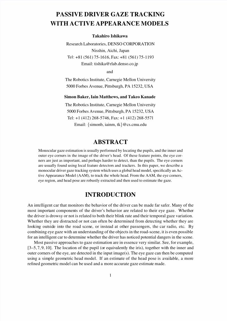
two shape modes (s1 and s2) of an AAM are shown in Figure 2(a)–(c).

The appearance of the AAM is defined within the base mesh s0. Let s0 also denote the set

of pixels u = (u, v)T that lie inside the base mesh s0, a convenient abuse of terminology. The

appearance of the AAM is then an image A(u) defined over the pixels u ∈ s0. AAMs allow

linear appearance variation. This means that the appearance A(u) can be expressed as a base

appearance A0(u) plus a linear combination of l appearance images Ai(u):

A(u) = A0(u) +l

i=1

λi Ai(u) (9)

where λi are the appearance parameters. As with the shape, the appearance images Ai are

usually computed by applying PCA to the (shape normalized) training images [2]. An example

of the base λ0 and first two appearance modes (λ1 and λ2) are shown in Figures 2(d)–(f).

Although Equations (8) and (9) describe the AAM shape and appearance variation, they do

not describe how to generate a model instance. The AAM model instance with shape param-

eters p and appearance parameters λi is created by warping the appearance A from the base

mesh s0 to the model shape mesh s. In particular, the pair of meshes s0 and s define a piece-

wise affine warp from s0 to s which we denote W(u;p). Three example model instances are

included in Figures 2(g)–(i). This figure demonstrate the generative power of an AAM. The

AAM can generate face images with different poses (Figures 2(g) and (h)), different identities

(Figures 2(g) and (i)), and different expressions, (Figures 2(h) and (i)).

5



(a) Base Shape s0 (b) 2D Shape Mode s1 (c) 2D Shape Mode s2

(d) Base Appearance λ0 (e) Appearance Mode λ1 (f) Appearance Mode λs2

(g) Example Model Instance (h) Example Model Instance (i) Example Instance

(j) 3D Base Shape s0 (k) 3D Shape Mode s1 (l) 3D Shape Mode s2

Figure 2: An example Active Appearance Model [2]. (a–c) The AAM base shape s0 and the first two

shape modes s1 and s2. (d–f) The AAM base appearance λ0 and the first two shape modes λ1 and λ2.

(g–i) Three model instances. (j–l) The base 3D shape s0 and the first two 3D shape modes s1 and s2.

Figure 3: Example driver head tracking results with an AAM. View in color for the best clarity.

REAL-TIME DRIVER HEAD TRACKING WITH AN AAM

Driver head tracking is performed by “fitting” the AAM sequentially to each frame in the input

video. Three frames from an example movie of a driver’s head being tracked with an AAM are

included in Figure 3. Given an input image I , the goal of AAM fitting is to minimize:

u∈s0

A0(u) +

li=1

λiAi(u) − I (W(u;p))

2=

A0(u) +l

i=1


2

(10)

simultaneously with respect to the 2D AAM shape pi and appearance λi parameters. In [6] we

proposed an algorithm to minimize the expression in Equation (10) that operates at around 230

frames per second. For lack of space, the reader is referred to [6] for the details.

6



Figure 4: Pose estimation results. The computed roll, pitch, and yaw are displayed in the top left.

ESTIMATING DRIVER HEAD POSE WITH AN AAM

The shape component of an AAM is 2D which makes driver head pose estimation difficult. In

order to extract the head pose, we also build a 3D linear shape model:

s = s0 +mi=1

pi si (11)

where the coefficients pi are the 3D shape parameters and s, etc, are the 3D shape coordinates:

s =

x1 x2 . . . xn

y1 y2 . . . ynz1 z2 . . . zn

. (12)

In [11] we showed how the equivalent 3D shape variation si can be computed from the corre-

sponding 2D shape variation si using our non-rigid structure-from-motion algorithm [12]. An

example of the 3D base shape s0 and the first two 3D shape modes (s1 and s2) of the AAM in

Figure 2 are shown in Figure 2(j)–(l). In order to combine this 3D model with the 2D model

we need an image formation model. We use the weak perspective imaging model defined by:

u = Px =

ix iy iz jx jy jz

x +

a

b

. (13)

where (a, b) is an offset to the origin and the projection axes i = (ix, iy, iz) and j = ( jx, jy, jz)are equal length and orthogonal: i · i = j · j; i · j = 0. To extract the driver head pose and AAM

scale we perform the AAM fitting by minimizing:

A0(u) +l

i=1


2

+ K ·s0 +

mi=1

pi si −P

s0 +

mi=1

pi si

2

(14)

simultaneously with respect to pi, λi, P, and pi, rather than using Equation (10). In Equa-tion (14), K is a large constant weight. In [11] we extended our 2D AAM fitting algorithm [6]

to minimize the expression in Equation (14). The algorithm operates at around 286Hz [11].

The second term enforces the (heavily weighted soft) constraints that the 2D shape s equals the

projection of the 3D shape s with projection matrix P. Once the expression in Equation (14)

has been minimized, the driver head pose and AAM scale can be extracted from the projection

matrix P. Two examples of pose estimation are shown in Figure 4.

7



(a) Eye Region Extraction (b) Initial Iris Estimate (c) Refined Iris Estimate

Figure 5: Example iris detection result: (a) Example eye corner tracking and eye region extraction re-

sults computed from an AAM fit. (b) The initial iris location and radius computed by template matching.

(c) The refined iris location and radius after edge-based ellipse fitting.

EYE CORNER TRACKING AND EYE REGION EXTRACTION

Once the AAM has been fit to an input video frame, it is easy to locate the eye corners and

extract the eye regions. The AAM has mesh vertices that correspond to each of the inner and

outer eye corners. The eye corner locations in the image can therefore be just read out of

W(s;p), the location of the AAM mesh in the images. See Figure 5(a) for an example.

In the AAM, each eye is modeled by six mesh vertices. It is therefore also easy to extract

the eye region as a box slightly larger than the bounding box of the six eye mesh vertices. If

(xi, yi) denotes the six mesh vertices for i = 1, . . . , 6, the eye region is the rectangle with

bottom-left coordinate (BLx, BLy) and top-right coordinate (T Rx, T Ry), where:

BLx

T Rx

BLy

T Ry

=

min xi

max xi

min yimax yi

+

−cxcx−dy

dy

. (15)

and (cx, dy) is an offset to expand the rectangle. Again, see Figure 5(a) for an example.

IRIS DETECTION

Once the eye region has been extracted from the AAM, we detect the iris to locate the center

of the iris. Our iris detector is fairly conventional and consists of two parts. Initially template

matching with a disk shaped template is used to approximately locate the iris. The iris location

is then refined using an ellipse fitting algorithm similar to the ones in [7, 10].

Template Matching

We apply template matching twice to each of the eye regions using two different templates.

The first template is a black disk template which is matched against the intensity image. The

second template is a ring (annulus) template that is matched against the vertical edge image.

The radius of both templates are determined from the scale of the AAM fit. The two sets of

matching scores are summed to give a combined template matching confidence. The position

of the pixel with the best confidence becomes the initial estimate of the center of the iris. In

Figure 5(b) we overlay the eye image with this initial estimate of the iris location and radius.

8



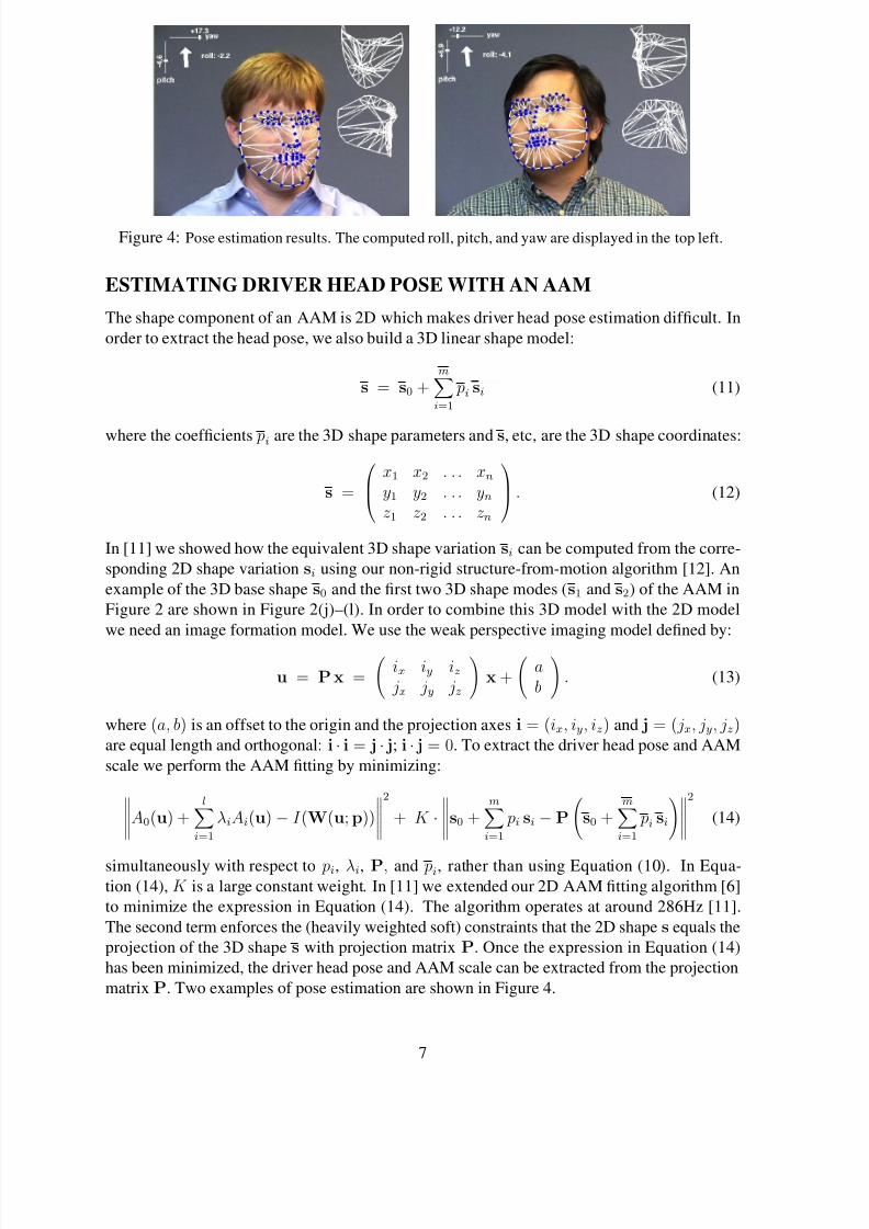
Figure 6: An example of head tracking with an AAM.

(a) Ground truth (20, 0, 0) (b) Ground truth (10, 0, 0) (c) Ground truth (0, 0, 0)

Result value (20,−1.8,−3.6) Result value (10, 2.0,−4.3) Result value (0.8,−1.8,−0.8)

Figure 7: Example pose (yaw, pitch, roll) estimation with the AAM.

Edge-Based Iris Refinement

The initial iris estimate is then refined as follows. First, edges are detected by scanning radially

from the initial center of the pupil outward. Next, an ellipse is fit to the detected edges to refine

the estimate of the iris center. Edges a long way away from the initial estimate of the radius

are filtering out for robustness. The ellipse is parameterized:

a1x2

+ a2xy + a3y2

+ a4x + a5y = 1 (16)

and the parameters a1, . . . , a5 are fit using least squares. This refinement procedure is repeated

iteratively until the estimate of the center of the iris converges (typically only 2-3 iterations are

required.) Example results are shown in Figure 5(c).

QUANTITATIVE EVALUATION IN THE LABORATORY

EYE CORNER TRACKING, POSE AND SCALE ESTIMATION

In Figure 6 we include three frames of a head being tracked using an AAM. Notice how thefacial features are tracked accurately across wide variations in the head pose. In Figure 7

we include three example pose estimates using the 3D AAM. Note that the yaw is estimated

particularly accurately. Besides the eye corner locations and the head pose, the other quantity

we extract from the AAM fit is the head scale S . We evaluate the scale estimate using the fact

that the scale is inversely proportional to the distance to the head (the depth.) In Figure 8 we

compute the distance to the head using the scale as the driver slides the seat back.

9



(a) depth:64.7cm (b) depth:67.4cm (c) depth:71.3cm (d) depth:74.0cm

(e) depth:75.7cm (f) depth:77.5cm (g) depth:78.7cm (h) depth:80.1cm

Figure 8: Verification of the scale estimated by the AAM. Since the scale is inversely proportional to

depth, we can use the scale to estimate the distance to the driver’s head. (a-h) The distance estimated

from the AAM scale increases smoothly as the seat is moved backward.

GAZE ESTIMATION

We collected a ground-truthed dataset by asking each subject to look in turn at a collection of markers on the wall. The 3D position of these markers was then measured relative to the head

position and the ground-truth gaze angles computed. We took multiple sequences with different

head poses. All variation was in the yaw direction and ranged from approximately -20 degrees

to +20 degrees relative to frontal. In Figure 9(a–c) we include an example frontal images for

each of 3 subjects. We overlay the image with the AAM fit and a line denoting the estimated

gaze direction. We also include close ups of the extracted eye regions and the detected iris. In

Figure 9(d–e) we plot the estimated azimuth gaze angle against the ground truth. The average

error is 3.2 degrees. The green line in the figure denotes the “correct answer.”

QUALITATIVE EVALUATION IN A REAL CAR

If there are two cameras in the car, one imaging the driver, the other imaging the outside world,

it is possible to calibrate the relative orientations of the camera by asking a person to look at

a collection of points in the world and then marking the corresponding points in the outside-

view image. The relative orientation can then be solved using least-squares. We performed

this experiment and then asked the subject to track a person walking outside the car with their

gaze. Three frames from a video of the results are shown in Figure 10. In Figures 10(a–c)

we display the exterior view. We overlay the estimated gaze direction with a yellow circle

than corresponds to a 5.0 degree gaze radius. In Figures 10(d–e) we include the corresponding

interior view of the driver overlaid with the AAM, the extracted eye regions, the detected iris,and the estimated gaze plotted as a line. As can be seen, the person always lies well inside the

circle, demonstrating the high accuracy of our algorithm.

Conclusion

We have presented a driver gaze estimation algorithm that uses an Active Appearance Model

[2] to: (1) track the eye corners, (2) extract the eye region, (3) estimate the scale of the face,

10



(a) Gaze of Subject 1 (b) Gaze of Subject 2 (c) Gaze of Subject 3

(d) Azimuth of subject 1 (e) Azimuth of subject 2 (f) Azimuth of subject 3

Figure 9:Gaze estimation. (a-c) Gaze estimates overlaid on the input image. We also include the

AAM, the extracted eye region, and the detected iris. (d-f) A comparison between the ground-truth

azimuth gaze angle and the angle estimated by our algorithm. The average error is 3.2 degrees.

and (4) estimate the head pose. The irises are detected in the eye region using fairly standard

techniques and the gaze estimated from the above information using a fairly standard geometric

model. The robustness and accuracy of our passive, monocular system are derived from the

AAM tracking of the whole head, rather than using a local feature based technique. Once the

eye corners have been located, finding the irises and computing the gaze are straightforward.

ACKNOWLEDGMENTS

The research described in this paper was supported by DENSO CORPORATION, Japan.

REFERENCES

[1] V. Blanz and T. Vetter. A morphable model for the synthesis of 3D faces. In Proceedings

of Computer Graphics, Annual Conference Series (SIGGRAPH), pages 187–194, 1999.

[2] T. Cootes, G. Edwards, and C. Taylor. Active appearance models. IEEE Transactions on

Pattern Analysis and Machine Intelligence, 23(6):681–685, June 2001.

[3] A. Gee and R. Cipolla. Determining the gaze of faces in images. Image and Vision

Computing, 30:63–647, 1994.

[4] J. Heinzmann and A. Zelinsky. 3-D facial pose and gaze point estimation using a robust

real-time tracking paradigm. In Proceedings of the IEEE International Conference on

Automatic Face and Gesture Recognition, pages 142–147, 1998.

11



(a) Exterior View Frame 78 (b) Exterior View Frame 634 (c) Exterior View Frame 687

(d) Interior View Frame 78 (e) Interior View Frame 634 (f) Interior View Frame 687

Figure 10: Mapping the driver’s gaze into the external scene. The driver was told to follow the person

walking outside in the parking lot. We overlay the external view with a yellow circle with radius cor-

responding to a 5.0 error in the gaze estimated. As can be seen, the person always lies well within the

circle demonstrating the accuracy of our algorithm.

[5] Y. Matsumoto and A. Zelinsky. An algorithm for real-time stereo vision implementation

of head pose and gaze direction measurement. In Proceedings of the IEEE International

Conference on Automatic Face and Gesture Recognition, pages 499–505, 2000.

[6] I. Matthews and S. Baker. Active Appearance Models revisited. International Journal of

Computer Vision, 60(2):135–164, 2004.

[7] T. Ohno, N. Mukawa, and A. Yoshikawa. FreeGaze: A gaze tracking system for everyday

gaze interaction. In Proceedings of the Symposium on ETRA, pages 125–132, 2002.

[8] S. Romdhani and T. Vetter. Efficient, robust and accurate fitting of a 3D morphable model.

In Proceedings of the International Conference on Computer Vision, 2003.

[9] P. Smith, M. Shah, and N. da Vitoria Lobo. Monitoring head/eye motion for driver alert-

ness with one camera. In Proceedings of the IEEE International Conference on Pattern

Recognition, pages 636–642, 2000.

[10] K. Talmi and J. Liu. Eye and gaze tracking for visually controlled interactive stereoscopic

displays. In Signal Processing: Image Communication 14, pages 799–810, 1999.

[11] J. Xiao, S. Baker, I. Matthews, and T. Kanade. Real-time combined 2D+3D active ap-

pearance models. In IEEE Conference on Computer Vision and Pattern Recognition,

2004.

[12] J. Xiao, J. Chai, and T. Kanade. A closed-form solution to non-rigid shape and motion

recovery. In Proceedings of the European Conference on Computer Vision, 2004.

12

ishikawa takahiro 2004 2

Documents