isogeometric boundary element methods for three ... · isogeometric boundary element methods for...
TRANSCRIPT

Available online at www.sciencedirect.com
ScienceDirect
Comput. Methods Appl. Mech. Engrg. ( ) –www.elsevier.com/locate/cma
Isogeometric boundary element methods for three dimensional staticfracture and fatigue crack growth
X. Penga, E. Atroshchenkob,∗, P. Kerfridena, S.P.A. Bordasc,d,a,e
a Institute of Mechanics Materials and Advanced Manufacturing, Cardiff University, CF24 3AA, UKb Department of Mechanical Engineering, University of Chile, Santiago, 8370448, Chile
c Universite du Luxembourg, Faculte des Sciences, de la Technologie et de la Communication, 6 rue Richard Coudenhove-Kalergi, L-1359,Luxembourg
d Research Unit in Engineering Science Campus Kirchberg, G 007, Luxembourge University of Western Australia, 35 Stirling Hwy, Crawley, WA 6009, Australia
Highlights
• We implement an isogeometric BEM routine for fracture by use of dual boundary integral equations.• We propose a singular integration scheme to improve the quadrature accuracy for elements with high aspect ratios.• We investigate the approaches to compute stress intensity factors based on a NURBS representation of the crack surfaces.• We outline a geometric algorithm to propagate the crack based on the fatigue Paris law.
Abstract
We present a novel numerical method to simulate crack growth in 3D, directly from the Computer-Aided Design (CAD)geometry of the component, without any mesh generation. The method is an isogeometric boundary element method (IGABEM)based on non-uniform rational B-splines (NURBS). NURBS basis functions are used for the domain and crack representation aswell as to approximate the physical quantities involved in the simulations. A stable quadrature scheme for singular integrationis proposed to enhance the robustness of the method in dealing with highly distorted elements. Convergence studies in the crackopening displacement is performed for a penny-shaped crack and an elliptical crack. Two approaches to extract stress intensityfactors (SIFs): the contour M integral and the virtual crack closure integral are compared using dual integral equations. The resultsshow remarkable accuracy in the computed SIFs, leading to smooth crack paths and reliable fatigue lives, without requiring thegeneration of any mesh from the CAD model of the component under consideration.c⃝ 2016 Elsevier B.V. All rights reserved.
Keywords: Isogeometric analysis; NURBS; Linear elastic fracture; Boundary element method; Crack growth; Fracture simulations directly fromCAD
∗ Corresponding author. Fax: +56 2 6896057.E-mail address: [email protected] (E. Atroshchenko).
http://dx.doi.org/10.1016/j.cma.2016.05.0380045-7825/ c⃝ 2016 Elsevier B.V. All rights reserved.

2 X. Peng et al. / Comput. Methods Appl. Mech. Engrg. ( ) –
1. Introduction
1.1. Damage tolerance assessment
The simulation of crack propagation is crucial in most areas of engineering and science. Predicting fracture iscentral to devising more durable and safer products and to understand natural phenomena.
We focus in this paper on one particular type of failure simulation known as ‘fatigue crack growth’ and whichoccurs in a variety of fields. When subjected to low amplitude cyclic loading, much below those causing significantunrecoverable plastic deformations, materials gradually damage which leads to crack initiation, propagation, and, inturn, to the subsequent global failure of the component.
In fatigue crack growth simulations, the goal is to estimate the number of cycles that a component can undergobefore it is unfit for purpose. Evaluating this ‘residual life’ requires the ability, to both compute the number of cyclesto initiation and to estimate the growth of a given crack given a number of loading cycles. We do not discuss the crackinitiation phase in this paper, but focus on the problem of simulating the growth of a crack whose initial geometry isknown. One of the widely used approaches to predict fatigue crack propagation consists in assuming that the materialaround the crack behaves in a linear elastic manner, compute the energy release rate, through the evaluation of stressintensity factors, and based on those, to estimate the amount of crack advance using empirical laws such as the Parislaw.
1.2. Simulating fatigue crack growth
Simulating (fatigue) crack growth leads to a number of requirements for the associated numerical methods1:
1. Computing the displacement and stress fields within the component during crack growth;2. Representing the crack surface as it grows;3. Estimating the energy release rate along the crack;4. Computing the crack propagation angle and crack propagation increment along the crack front.
Point 1. is complicated by the singularity of the stress field along the crack front, which requires dense meshes to begenerated and regenerated as the crack grows. Point 2. requires the numerical method to deal with the propagatingdisplacement discontinuity across the crack faces, as those evolve. Point 3. assumes the ability of the method toaccurately evaluate stress intensity factors (SIFs). In this paper, we consider two approaches to do so, which aredetailed later in the manuscript. The crack growth direction and increment (Point 4.) is provided by the crack growthlaw. We assume in the following that the crack grows in the direction which maximizes the tangential stress (hoopstress). We use Paris’ law to compute the increment in crack growth along the crack front. We focus in the rest of thisintroduction on points 1. and 2. only, for which a number of methods have been proposed over the years. Points 1. and2. above represent the major challenge for numerical fracture modeling, i.e. the combined requirement of simulatingevolving discontinuities and singularities. This requires meshes used in the finite element method to be generated andregenerated as the crack grows and to use special elements relying, e.g. on Barsoum elements [2] to represent thesingularity. This difficulty is compounded by the fact that the cracks are typically two or more orders of magnitudesmaller than the component itself which exacerbates the meshing difficulty by leading to large gradients in elementsize.
In spite of these challenges, the finite element method (FEM) has been used rather widely to simulate the crackpropagation directly with certain adaptive re-meshing operation [3–5]. Some commercial software packages such asADAPCRACK, ZENCRACK and FRANC3D have been developed based on this idea [6–8] and two recent reviewpapers can be consulted for details [1,9]. The complexity of remeshing, in spite of tremendous recent progress inDelaunay triangulation [10] and other meshing procedures [11], re-meshing remains a difficult problem when multiplecracks are interacting or for geometrically complex components where the presence of cracks as internal boundariessignificantly constrain the mesh generation and regeneration process.
1 Note that because realistic industrial problems are three dimensional, we will not consider methods which have been developed only fortwo-dimensional crack propagation. We refer the reader to a recent review on 3D crack growth for some details which are not included in theforthcoming literature review [1].

X. Peng et al. / Comput. Methods Appl. Mech. Engrg. ( ) – 3
Partition of unity enrichment volume-based methods. Another approach is to introduce cracks through enrichmentfunctions using the partition of unity method [12]. This was first done in a method called the ‘extended finite elementmethod’ [13] and the ‘generalized finite element method’ [14,15] which are both relying on the idea of multiplying thestandard shape functions by enrichment functions which ‘know’ about the nature of the solution. Whilst enrichmentitself is an idea dating back to the 1970’s [16], and is also found in the meshfree literature since the early 1990’s [17]2
partition of unity enrichment enables a local enrichment of the basis, leading to banded matrices and enabling toflexibly combine different enrichments within a single computational domain. This final point is particularly importantas enrichment locality is required to enable the simulation of multiple crack fronts.
In practice, partition of unity (PU) enrichment is an effective approach to somewhat alleviate the meshingand remeshing burden in fracture modeling [13–15]. Additional enrichment functions are used to both introducedisplacement discontinuities and stress singularities into the model. This enables to introduce the cracks quasi-independently of the background mesh. This flexibility simplifies local adaptive processes, as the regenerated meshneed not conform to the crack faces [19–21] does not come for free, as (1) numerical integration requires specialattention [22–24]; (2) optimal convergence requires enriching a volume independent of the mesh size, therebydeteriorating the condition number [25–27]; (3) since the mesh does not conform to the crack, the latter must berepresented geometrically through another approach. Usually, enrichment is coupled with level set methods [28] usedto represent the crack surfaces implicitly. This has been used for 3D crack growth problems [29–31,27] as well asfor industrial applications [32,21,33]. A special case of partition of unity methods, meshfree methods have also beenproposed with the aim of further reducing the mesh burden, for example, the element-free Galerkin (EFG) [34], theextended EFG [35,36], the cracking-particle method [37] etc. For more details, the readers could refer the reviewpaper on meshfree methods and their implementation, by Nguyen et al. [18] and the review paper on partition of unitymethods for fracture in [1].
Boundary-based methods. Another approach is to model cracks by boundary-based methods such as the boundaryelement method (BEM) or the scaled boundary finite element method (SBFEM).
Boundary element methods can be collocation or Galerkin-based. For problems without body forces or internalvariables, the discretization of the boundary is sufficient to approximate the field variables. When cracks evolve, onlythe boundary surfaces are updated which does not require the regeneration of a volume mesh. Several additionaldifficulties come with the flexibility brought by boundary-based methods.
1. The fundamental solution to the problem at hand must be known, which limits the applicability to the methodrather severely. However, for many industrial damage tolerance problems, linear elastic fracture is used, whichmakes boundary-based methods generally applicable.
2. Particular care is required to deal with the fact that the cracks are zero-thickness surfaces, which leads tooverlapping collocation points and thus identical equations. To avoid the resulting singularity in the systemmatrix, Hong and Chen [38] proposed the dual boundary integral representations by introducing the hyper-singularequation derived from the secondary field [39].
3. Numerical integration is complicated, due to the emergence of hyper-singular terms in the integrals. However, anumber of methods have been proposed to deal with these singularities. The most common ones are singularitysubtraction techniques (used in this paper) and regularization of the boundary integral equations[40,41].
4. The resulting system matrices are full. This makes the solution of the system of equations slow. However, this isnot specific to fracture mechanics and approaches have been proposed to accelerate the solution process [42].
The use of dual boundary integral equations makes the crack propagation simulation more effective through a singledomain. And the corresponding dual BEM was subsequently implemented for 2D and 3D fracture [43–45] and wasextended to material-nonlinear fracture [46,47] and dynamic crack propagation [48]. Commercial packages based onBEM are BEASY [49] and FRANC3D [8]. Apart from the dual BEM based on the collocation method, the GalerkinBEM, in particular the symmetric Galerkin BEM (SGBEM) has also drawn attention for fracture analysis [50–52].The symmetric matrix system of SGBEM also facilitates the coupling with FEM [53,54].
An interesting hybrid approach was proposed named scaled boundary finite element method (SBFEM) by Song andWolf [55]. Only the boundary of the domain is needed for discretization in analysis without fundamental solution. Thus
2 [18] provides a review of enrichment methods, comparing intrinsic and extrinsic partition of unity enrichment. Another review is providedin [1], which focuses on fracture simulations using partition of unity methods.
4 X. Peng et al. / Comput. Methods Appl. Mech. Engrg. ( ) –
the computational efficiency is improved by reducing the spatial dimension by one while the integration is efficientas well since no singular integration is introduced as in BEM. Natarajan et al. enhanced isogeometric analysis by theSBFEM, providing a method which inherits advantages of both FEM and IGABEM. Nevertheless, the approach doesrequire a certain subdivision of the domain for complex geometries in order to obtain the scaling center [56].
1.3. Dealing with component complexity
Design cycle. Practical damage-tolerant engineering design requires typically a large number of iterations betweendesigners on the one hand and stress and fatigue analysts on the other. The former group of engineers provide aninitial design, which is refined iteratively through successive stress analyses and fracture propagation simulationsunder fatigue. The usual approach is to generate a mesh for stress analysis, compute the most highly stressed regionsin the component and introduce a crack of dimensions defined by design codes at the location of maximum principletensile stress in the component (this requires generating a new mesh, where the elements are typically several ordersof magnitude smaller in size than the original stress analysis mesh). The crack is grown from this initial flaw and thenumber of cycles to fatigue is estimated. If the component’s fatigue life happens to be unsatisfactory, the design ismodified, and the whole process is repeated. It is clear that this approach is inefficient in terms of human intervention,slow, expensive and non-robust, since a typical design iteration can take as much as a few months for a relativelysimple component.
Isogeometric analysis. Isogeometric analysis (IGA), first introduced by Hughes et al. [57] aims at enabling theengineer to use the same approximation functions to describe both the geometry of the component (provided byComputer Aided Design tools) and the solution of the problem (the displacement and stress fields in the present case).In its original, finite element based form, IGA does not completely suppress the need to create a mesh, as the CADdata provides only a ‘shell’ for the component, but gives no information about the parametrization of the interior ofthe volume which it encloses. Although the finite element version of IGA was used for fracture analysis [58–61]. Thismotivated the inception of a boundary element version of IGA for elasticity problems in [62–64].
Isogeometric boundary element methods: stress analysis directly from CAD. The conjoint use of IGA and BEM(IGABEM) permits the direct use of the CAD model, without any mesh generation and was developed for stressanalysis [63,62,64], shape optimization [65–67]. This approach provides a tight and seamless transition between CADand stress analysis. IGABEM has thus been subsequently extended to many fields [68–71]. PU enriched IGABEMwas later proposed in [72,73] and trimmed NURBS approaches were presented in [74,75]. Accelerated solutionswere proposed in [42] and Galerkin version of IGABEM in [76,77] etc. The benefit of smoothness to boundaryintegrals (BIEs) brought by IGA was recently investigated in [78]. Recently the isogeometric SGBEM has beenapplied for 2D fracture mechanics [79]. However, most work known to us primarily focuses on 2D problems, whichare inconsequential for practical engineering applications. Indeed, the generation of analysis-suitable 3D volumeparametrization for complex geometries is still an open question [80–82].
Based on the above discussion, the goal of our contribution is to investigate the advantages and drawbacks ofisogeometric collocation boundary element methods for linear elastic fracture. In particular, we investigate:
1. How the higher-order continuity of the spline basis improves the accuracy of the stress field near the crack tip,crucial in fracture analysis and how this impacts the required number of degrees of freedom compared to a C0 ordiscontinuous Lagrange basis;
2. The preservation and continuity of the curvature, tangential and normal vectors along the crack front during crackgrowth and evolved thanks to the exact representation of curved cracks;
3. The advantages of constructing a local crack front system directly based on the spline-based curve or surface-represented cracks and the impact of this direct construction on the accuracy of the fracture parameters;
4. The lack of volume parametrization/reparametrization for crack initiation and propagation. The cracks are modeledby spline surfaces directly as external boundaries of the geometry.
In short, we explore the qualities of IGABEM for 3D fracture analysis and fatigue crack growth. We use dual integralequations to model cracks, a local singularity removing technique proposed by Guiggiani [83] is applied on the variousorders of singular integrals (up to hyper-singular O(1/r3)), and its improved version is tailored to handle distortedelements (or elements with high aspect ratio) which commonly arise in isogeometric based methods. The crack is

X. Peng et al. / Comput. Methods Appl. Mech. Engrg. ( ) – 5
Fig. 1. Crack model.
explicitly represented by a NURBS surface as an internal boundary and an algorithm is outlined to describe the crackpropagation such that the smoothness in geometry brought by IGA and in the solution brought by BEM is fullyleveraged for extracting the stress intensity factors and simulating crack growth.
Outline of the paper. The rest of the paper is organized as follows. Section 2 briefs the boundary integral equations(BIEs) that applied in fracture modeling. Section 3 illustrates the NURBS basis functions on 2D surfaces and thecollocation scheme. Section 4 outlines the improved singular integration based on the singularity subtraction technique[83]. The crack growth related work is detailed in Section 5, including updating the crack surface geometrically,computing the stress intensity factors and the fatigue fracture rule: the Paris law. Numerical examples for both staticfracture analysis and crack growth are given in Section 6. We conclude our work and propose the future research ofinterest in the last section.
2. Boundary integral equations for crack modeling
Consider an arbitrary domain Ω which contains a crack as in Fig. 1. The boundary of the domain Γ = Sr ∪Sc+∪Sc− ,where the non-crack boundary Sr is composed of Su where Dirichlet boundary conditions are prescribed (knowndisplacements u), St where Neumann boundary conditions are prescribed (known tractions t). The displacement BIEis given by finding u and t such that
ci j (s)u j (s) =
Γ
Ui j (s, x)t j (x)dS(x)− −
Γ
Ti j (s, x)u j (x)dS(x), (1)
where the Ui j , Ti j are called fundamental solutions and, for linear elasticity,
Ui j (s, x) =1
16πµ(1 − ν)r
(3 − 4ν)δi j + r,ir, j
, (2)
Ti j (s, x) = −1
8π(1 − ν)r2
∂r
∂n[(1 − 2ν)δi j + 3r,ir, j ] − (1 − 2ν)(r,i n j − r, j ni )
, (3)
where µ = E/[2(1+ν)], E is Young’s Modulus and ν Poisson’s ratio. s is the source point (or collocation point. Thistwo terms will be used interchangeably in the remainder part of this paper). −
denotes the integral is interpreted in the
Cauchy Principal Value sense. The traction BIE is obtained by differentiation of the displacement BIE with respect tos and multiplication by the elastic tensor Ei jkl :
ci j (s)t j (s) = −
Γ
Ki j (s, x)t j (x)dS(x)− =
Γ
Hi j (s, x)u j (x)dS(x), (4)
Hi j (s, x) = Eikpq∂Tpj (s, x)∂sq
nk(s), Ki j (s, x) = Eikpq∂Upj (s, x)
∂sqnk(s), (5)
where =
denotes the Hadamard Finite Part integral. ci j is called a jump term and on a smooth boundary ci j = 0.5δi j .

6 X. Peng et al. / Comput. Methods Appl. Mech. Engrg. ( ) –
The idea of the boundary element method is to discretize the boundary geometry and the physical fields using setsof basis functions. Subsequently, the source point is placed at the collocation points and the displacement BIE in Eq.(1) or traction BIE (4) is transformed into a system of linear algebraic equations. However, when the domain containsa crack, the collocation points on the overlapping surfaces Sc+ and Sc− could coincide (refer to Fig. 1(b)). The systemmatrix becomes then singular. Two ways to deal with this problem are given in the following sections.
2.1. Dual equations
The difficulty caused by the collapsed crack surfaces is circumvented through the use of dual equations, byprescribing different BIEs on either face of the crack. The displacement BIE (Eq. (1)) is used on one face (Sc+ )and on the non-crack boundary Sr . The traction BIE (Eq. (4)) is used on the other crack face (Sc− ). For the collocationpoint s+ on the crack surface Sc+ , Eq. (1) can be rewritten as,
ci j (s+)u j (s+)+ ci j (s−m)u j (s−
m) =
Sr
Ui j (s+, x)t j (x)dS(x)−
Sr
Ti j (s+, x)u j (x)dS(x)
− −
Sc+
Ti j (s+, x+)u j (x+)dS(x)− −
Sc−
Ti j (s−m, x−)u j (x−)dS(x)
+
Sc+
Ui j (s+, x+)t j (x+)dS(x)+
Sc−
Ui j (s−m, x−)t j (x−)dS(x). (6)
Analogously, the traction BIE (Eq. (4)) on the other crack surface (Sc− in Fig. 1(b)) becomes,
ci j (s−)t j (s−)+ ci j (s+m)t j (s+
m) =
Sr
Ki j (s−, x)t j (x)dS(x)−
Sr
Hi j (s−, x)u j (x)dS(x)
− =
Sc−
Hi j (s−, x−)u j (x−)dS(x)− =
Sc+
Hi j (s+m, x+)u j (x+)dS(x)
+ −
Sc−
Ki j (s−, x−)t j (x−)dS(x)+ −
Sc+
Ki j (s+m, x+)t j (x+)dS(x). (7)
s−m denotes the mirror point of s+ on Sc− , which means s−
m and s− share the same physical and parametric coordinatesbut their normal vectors are opposite. The last two terms of both equations and left hand side of Eq. (7) are omitteddue to the traction-free crack.
Remark. Due to the collapsed boundary, two jump terms arise in each BIE and each operator not only exhibitssingularity on the crack surface where the collocation points are located, but also on the one where the mirror pointsof the collocation points are located.
2.2. Crack opening displacement (COD) equation
The boundary integral equation for crack problem can also be reformulated by setting the boundary quantity ascrack opening displacement over a couple of crack surfaces. Let the source point approach one crack surface, forexample Sc = Sc+ , and note that n = n+
= −n−, we have:
ci j (s+)u j (s+)+ ci j (s−m)u j (s−
m) =
Sr
Ui j (s+, x)t j (x)dS(x)− −
Sr
Ti j (s+, x)u j (x)dS(x)
+
Sc
Ui j (s+, x+)(t j (x+)+ t j (x−))dS(x)
− −
Sc
Ti j (s+, x+)(u j (x+)− u j (x−))dS(x). (8)

X. Peng et al. / Comput. Methods Appl. Mech. Engrg. ( ) – 7
The corresponding traction BIE is:
ci j (s+)t j (s+)+ ci j (s−m)t j (s−
m) = −
Sr
Ki j (s+, x)t j (x)dS(x)− =
Sr
Hi j (s+, x)u j (x)dS(x)
+ −
Sc
Ki j (s+, x+)(t j (x+)+ t j (x−))dS(x)
− =
Sc
Hi j (s+, x+)(u j (x+)− u j (x−))dS(x). (9)
Eq. (9) can be used alone if the COD alone will be used as the unknown for the fatigue crack growth problem. Howeverif the displacement field needs to be known on the crack surfaces, Eq. (8) should also be solved. For a infinite domain(Sr → ∞), assuming that traction-free crack faces are assumed, we arrive at:
0 = t∞j (s)− =
Sc
Hi j (s, x)[[u j (x)]]dS(x). (10)
[[u j (x)]] = u j (x+) − u j (x−) is the crack opening displacement. All the subscripts ‘+’ are omitted since the integralis only over a single crack surface. t∞ is interpreted as the solution in the ‘no crack’ space.
3. NURBS discretization and collocation
NURBS basis functions are a generalization of B-spline functions that allows a ‘projection’ from square and cubicdomains to form general geometries. B-spline basis functions are defined over a knot vector, which is a non-decreasingsequence of real numbers given in the parameter space. A knot vector is denoted as Ξ = ξ1, ξ2, . . . , ξn+p+1, whereξi ∈ R is the i th parameter coordinate (knot), p is the order of the polynomial, n is the number of the basis functions.For a given order p, the B-spline basis functions Ni,p with 1 6 a 6 n are defined by the Cox–de Boor recursion:
Ni,0(ξ) =
1 ξi 6 ξ < ξi+10 otherwise,
(11)
then, for p > 0,
Ni,p(ξ) =ξ − ξi
ξi+p − ξiNi,p−1(ξ)+
ξi+p+1 − ξ
ξi+p+1 − ξi+1Ni+1,p−1(ξ). (12)
The continuity of B-spline basis functions at ξi can be decreased by repeating the knot several times. If ξi hasmultiplicity k (ξi = ξi+1 = · · · = ξi+k−1), then the basis functions are C p−k continuous at ξi . Particularly, whenk = p, the basis is C0 and k = p + 1 leads to a discontinuity at ξi . If the first and last knot have k = p + 1, the knotvector is called an open knot vector. More details can be found in [84,60].
Given the knot vectors Ξ = ξ1, ξ2, . . . , ξn+p+1 and H = η1, η2, . . . , ηm+q+1, and the control points net Pi, j .The B-spline surface S(ξ, η) is given by the tensor-product of B-spline basis functions defined in the 2D parametricdomain [ξ1, ξn+p+1] × [η1, ηm+q+1],
S(ξ, η) =
ni=1
mj=1
Ni,p(ξ)M j,q(η)Pi, j , (13)
where Ni,p(ξ)M j,q(η) are the 2D B-spline basis functions. The NURBS basis functions can be constructed byrationalizing the tensor-product B-spline basis functions as
Ri, j (ξ, η) =Ni,p(ξ)M j,q(η)wi, j
nk=1
ml=1
Nk,p(ξ)Ml,q(η)wk,l
, (14)
where the scalar variable wi, j is the weight associated with the control point Pi, j . For the sake of integration,the 2D NURBS basis functions are usually calculated in the element defined by the non-zero knot intervals[ξi , ξi+1] × [η j , η j+1] where the Gaussian rule can be applied [57].

8 X. Peng et al. / Comput. Methods Appl. Mech. Engrg. ( ) –
In the NURBS based isogeometric concept, the physical field is approximated by the same NURBS basis functionsas those used to describe the geometry Γ = Sr (ξ, η) ∪ Sc+(ξ, η) ∪ Sc−(ξ, η) = ∪
Nee=1 Se(ξ, η), Ne is the number of
NURBS elements. The displacement and traction fields can be approximated as follows:
ui (ξ, η) =
nA=1
RA(ξ, η)dAi , (15)
ti (ξ, η) =
nA=1
RA(ξ, η)qAi , (16)
where n = (p + 1)(q + 1) is the number of NURBS basis functions for an element and the construction of themap between the global index A and the local index (i, j) can be found in [57]. And di , qi are displacement andtraction control variables respectively. The parameter domain of an element [ξi , ξi+1] × [η j , η j+1] is converted into[−1, 1]×[−1, 1], which is called the parent space. We define ξ(ξi = ξ, η) as the parameter coordinate and ξ(ξi = ξ , η)
as the parent coordinate of the field point x, and J = J (ξ , η) is the Jacobian transformation from physical to parentspace. The transformation for a NURBS element from parameter to parent space is
ξ =(ξi+1 − ξi )ξ + (ξi+1 + ξi )
2,
η =(ηi+1 − ηi )η + (ηi+1 + ηi )
2,
J =dS
dξ(ξi+1 − ξi )
2+
dS
dη(ηi+1 − ηi )
2,
(17)
where dSdξ and dS
dη are calculated from Eq. (13). Substituting the discretized displacements and tractions into the BIEs(6) and (7) will give,
nI=1
C Ii j (s
+)d+,Ij +
nI=1
C Ii j (s
−m)d
−,Ij =
Se⊂Sr
nI=1
U Ii j q
Ij −
Se⊂Sr
nI=1
T Ii j d
Ij
−
Se⊂Sc+
nI=1
T Ii j d
+,Ij −
Se⊂Sc−
nI=1
T Ii j d
−,Ij
+
Se⊂Sc+
nI=1
U Ii j q
+,Ij +
Se⊂Sc−
nI=1
U Ii j q
−,Ij (18)
nI=1
C Ii j (s
−)q−,Ij +
nI=1
C Ii j (s
+m)q
+,Ij =
Se⊂Sr
nI=1
K Ii j q
Ij −
Se⊂Sr
nI=1
H Ii j d
Ij
−
Se⊂Sc−
nI=1
H Ii j d
−,Ij −
Se⊂Sc+
nI=1
H Ii j d
+,Ij
+
Se⊂Sc−
nI=1
K Ii j q
−,Ij +
Se⊂Sc+
nI=1
U Ii j q
+,Ij (19)
where the jump term and integrals of the fundamental solutions are respectively written as:
C Ii j (s) = ci j RI (ξ s), (20)
F Ii j =
Se
Fi j (s, x(ξ))RI (ξ) J (ξ)dS, F can be T,U, H, K . (21)
Note that the discretization process of the singular integrals will lead to singular elements (s ∈ Se) and non-singularelements (s ∈ Se). The numerical quadrature for them needs to be treated separately. Let us take the kernel H with
X. Peng et al. / Comput. Methods Appl. Mech. Engrg. ( ) – 9
hyper-singular term for example, if s = s+∈ S+
e0:
H Ii j = =
Se
Hi j (s+, x+(ξ))RI (ξ)J (ξ)dS, if Se = S+
e0;
H Ii j = =
Se
Hi j (s−m, x−(ξ))RI (ξ)J (ξ)dS, if Se = S−
m,e0, the mirror element of S+
e0;
H Ii j =
Se
Hi j (s+, x(ξ))RI (ξ)J (ξ)dS, if Se ⊂ Γ − S+
e0 − S−
m,e0.
(22)
The discretized COD equation (10) can be obtained in a similar way and its implementation is simpler as only onecrack face is used and the singularity in the ‘mirror’ element does not appear.
The Greville abscissae (GA) has been used to generate the collocation points. In IGA, the number of controlpoints in the geometry representation has to be equal to the number of control variables in the field approximation,which requires the same number of collocation points. For domains with continuous parametrization, composed bytrimless and compatible NURBS patches, the number of collocation points obtained by the Greville abscissae is equalto the number of control points in the geometry representation, which is suitable for approximation of continuoussolutions. However, in some cases the collocation points, generated by the GA may not be suitable for the analysis.For example, for the geometries with sharp edges or corners, the discontinuous tractions can be better approximatedby the discontinuous basis functions, which can be obtained from the original geometry parametrization by doublingthe knot values and the corresponding control points. Or for the geometries parametrized by degenerated elements,when the number of the collocation points generated by the GA does not match the number of control variables inthe solution approximation. In order to match the number of discontinuous basis functions, the collocation points areshifted inside an element by an offset α by:
ξs,i = ξs,i + α(ξs,i+1 − ξs,i ), orξs,i = ξs,i − α(ξs,i − ξs,i−1), 0 < α < 1.
(23)
In this work, the knot values and control variables are doubled in order to approximate the traction fields. Whileflexible choices can be made to perform more efficient mesh refinement related to the geometry independent fieldapproximation, see [42]. We take α = 0.5 without particularly specified. We will show in the numerical example thatthe closer to 0 the value of α is, the more accurate the approximation will be. However, a smaller α will evoke stronger‘near-singularity’ in the neighborhood elements. Further improvements to overcome this difficulty will be pursued inthe future work.
4. Numerical integration
Due to the singularities in BIEs, there will be singular integration and non-singular integration after discretization.For the element containing the collocation point, singular integration is performed and in view of this, the element iscalled ‘singular’. Elements which exclude the collocation point are called non-singular elements. Singular integrationneeds to be carefully treated in BEM. Various numerical methods have been proposed, and one can refer to a reviewwork in [39]. A robust technique developed in [41] can be applied to regularize all the singular terms, i.e. transformthem into weakly singular terms via the use of simple solution of BIE. The regularization technique based on simplesolutions has been further developed in the framework of IGABEM [68,85,78]. However, this method fails whendealing with open surfaces such as cracks because of the existence of two jump terms in collapsed boundary [86].In the present work, we use the singularity subtraction technique (SST) proposed by Guiggiani [86,83] to removethe singularities arising in both BIEs. The SST is a method for the treatment of singular integrals regardless of meshdiscretization and proved to be efficient for fracture via dual BEM [44].
4.1. Singularity subtraction technique (SST) for singular integrals
The SST transforms various orders of singular integration into a weakly singular one based on the intrinsiccoordinate system of the singular element after discretization. Then the weakly singular integration becomes regular ifthe quadrature is performed in polar coordinates. By expanding the integrand into a series with respect to the intrinsic

10 X. Peng et al. / Comput. Methods Appl. Mech. Engrg. ( ) –
Fig. 2. Transformation between coordinate system for SST.
coordinates, the singularity can be represented explicitly with respected to the parametric distance between the sourcepoint and field point ρ. Then the singular terms are subtracted from the integrand, leaving the remaining to be regularfor which regular Gaussian rule is applied. The subtracted terms are added back semi-analytically. For example, forthe hyper-singular integral of the form
I = =
Se
H(s, x(ξ))R(ξ) J (ξ)dS, (24)
the polar coordinates ρ(ρ, θ) centered at the source point are introduced in the parent space (Fig. 2). The parentdomain is subdivided into triangles for quadrature. For each field point ξ in the sub-triangles, we have
ξ = ξs + ρ cos θ,
η = ηs + ρ sin θ. (25)
After the polar coordinate transformation, Eq. (24) becomes
I = limε→0
2π
0
ρ(θ)
α(ε,θ)
H(ρ, θ)R(ρ, θ) J (ρ, θ)ρdρdθ, (26)
where ρ(θ) = h/ cos θ . h is the shortest distance from the source point to the element edge and θ is the angle fromperpendicular direction to the field point as in Fig. 2. If we define θ0 as the angle of the perpendicular line, then theangle to the field point can be computed as
θ = θ + θ0. (27)
The integrand F(ρ, θ) = H(ρ, θ)R(ρ, θ) J (ρ, θ)ρ is expanded as:
F(ρ, θ) =F−2(θ)
ρ2 +F−1(θ)
ρ+ F0(θ)+ F1(θ)ρ + F2(θ)ρ
2+ · · · =
∞i=−1
Fi (θ)ρi . (28)
The first two singular terms on the right hand side are subtracted and added back semi-analytically, resulting in:
I = I1 + I2,
I1 =
2π
0
ρ(θ)
0
F(ρ, θ)−
F−2(θ)
ρ2 −F−1(θ)
ρ
dρdθ,
I2 =
2π
0I−1(θ) ln
ρ(θ)
β(θ)dθ −
2π
0I−2(θ)
γ (θ)β2(θ)
+1ρ(θ)
dθ,
(29)
where I1 is regular and I2 are regular line integrals, Both can be applied with Gaussian quadrature rule. The evaluationof α(ε, θ), β(θ) and γ (θ) as well as the limiting process can be found in [83].

X. Peng et al. / Comput. Methods Appl. Mech. Engrg. ( ) – 11
4.2. Conformal mapping for SST
It has been revealed by Rong et al. [87] that the expansion coefficients Fi (θ) in Eq. (28) exhibits various ordersof near-singularity in the angular θ direction, although the singularity in the radial ρ direction disappears. This near-singularity is sensitive to the shape of the element and becomes severe when the element is highly distorted. The Fi (θ)
can be represented as [87]:
Fi (θ) =Fi (θ)
Ap(θ)=
Fi (θ)
[0.5(|ms1|
2 + |ms2|
2)(ω sin(2θ + ϕ)+ 1)]p/2 , (30)
where Fi (θ) are the regular trigonometric functions and integer ‘p’ is the order associated with ‘i’. The curvilinearbasis vectors ms
i = mi |ξ=ξ s, (i = 1, 2) are calculated as:
m1 =
∂x
∂ξ,∂y
∂ξ,∂z
∂ξ
,
m2 =
∂x
∂η,∂y
∂η,∂z
∂η
.
(31)
We introduces two parameters
λ = |ms1|/|m
s2|,
cosψ = ms1 · ms
2/|ms1||m
s2|,
(32)
such that
ϕ = arctanλ2
− 12λ cosψ
,
ω =
1 −
4 sin2 ψ
(λ+ λ−1)2< 1.
(33)
It can be concluded that when the element aspect ratio is large or the angle between two basis vectors tends to 0 or π(sinψ → 0), A(θ) will tend to 0, resulting in the near-singularity of Fi (θ). Both scenarios indicate a distorted shapeof the singular element, which are common in isogeometric analysis.
Rong et al. [87] constructed the conformal mapping from the parent space (ξ , η) to a new parametric space (ξ , η)where the two curvi-linear basis vectors in the new parametric space are orthogonal and have identical length, i.e.
ms1 · ms
2 = 0,
|ms1| = |ms
2|.(34)
Then A(θ) becomes a constant, which makes the integration nonsensitive to the element shape, if the series is expandedin the new space. The quadrature for the singular integral turns to be stable regardless of mesh distortion.
The mapping proposed by Rong et al. is tailored for triangular element, in this work we extend it to the quadrilateralelements (Fig. 2). In [87], the Jacobian transformation matrix T from ξ = (ξ , η) to a new parametric space ξ = (ξ , η)
is
T =
1 δ10 δ2
, so that ξ = Tξ , (35)
where δ1 = cosψ/λ, δ2 = sinψ/λ. Then the new basis vectorsms
1 ms2
=
ms
1 ms2
T−1
=ms
1 −(δ1/δ2)ms1 + (1/δ2)ms
2
(36)
12 X. Peng et al. / Comput. Methods Appl. Mech. Engrg. ( ) –
will satisfy the relation in Eqs. (34). The bilinear interpolation is used from (ξ , η) to the new parametric space (ξ , η)for a quadrilateral element:
ξ =
4I=1
NI (ξ)ξI,
N1(ξ , η) = 0.25(1 + ξ )(1 + η),
N2(ξ , η) = 0.25(1 − ξ )(1 + η),
N3(ξ , η) = 0.25(1 − ξ )(1 − η),
N4(ξ , η) = 0.25(1 + ξ )(1 − η).
(37)
Combining Eqs. (35) and (37), the nodal coordinates ξI
can be obtained as ξ1(1 + δ1, δ2), ξ
2(−1 + δ1, δ2),
ξ3(−1 − δ1,−δ2) and ξ
4(1 − δ1,−δ2). It should be noted that since 0 < ψ < π , δ2 > 0, the quadrilateral element is
guaranteed to have positive area (one possible plot is shown in Fig. 2). This requires the source point to be located atthe degenerated point in the geometry where |ms
i | = 0.It can be seen from Fig. 2 that the shape of the element in conformal space is controlled by the coefficients δ1 and
δ2. This means that if λ (reflecting the element aspect ratio) and cosψ (reflecting the element distortion) deviate from1, the conformal element will be skewed. This will result in sub-triangles with θ approaching ±π/2 if the field pointis close to the edges adjacent to the source point of the sub-triangles (Fig. 2). Thus ρ(θ) = h/ cos θ is not calculatedaccurately. To alleviate this near singularity in ρ(θ), the following Sigmoidal transformation is applied in the angulardirection such that the integration points will be adaptively clustered close to the edges where the near-singularity issevere, according to the value of θ [87],
w(θ) =1π
θ +
π
2
, −
π
2< θ <
π
2, 0 < z < 1,
z = z(s) = w(θ1)+12(s + 1)(w(θ2)− w(θ1)), −1 < s < 1, 0 ≤ z(θ1) < z < z(θ2) ≤ 1
f (z) =zm
zm + (1 − z)m,
θ = π f (z)−π
2,
J−1(θ) =∂θ
∂s=π [w(θ2)− w(θ1)]m f (z)m−1
2( f (z)m + (1 − f (z))m)2,
(38)
where s is the Gauß point from interval (−1, 1), the relation of θ and θ can be found in Eq. (27).
4.3. Numerical quadrature
In our numerical implementation, a Gaussian rule is applied in both radial and angular direction. Combining withthe study in [87] and our numerical tests of singular integration for NURBS elements (which are not presented in thepaper for brevity), we use 6 Gauß points are used in the radial direction, 18 Gauß points in the angular direction of eachsub-triangle for conformal SST unless otherwise specified. For each non-singular element, an adaptive subdivisionscheme is used according to the relative distance between the element and collocation point. All the rules are usedempirically without any error control algorithm.
5. Crack growth
The approaches used to represent and track the crack propagation can be classified into two manifolds, implicit andexplicit methods. A typical application of the former method would be the level set method [88] which was coupled inthe XFEM/GFEM to represent and grow the discontinuity [30,31]. The level set function is a signed distance functionto the crack surface defined on the underlying mesh, which could be either consistent with the mesh discretization
X. Peng et al. / Comput. Methods Appl. Mech. Engrg. ( ) – 13
of the problem or an independent structured mesh. Since the cracks are open surfaces, one more level set function,perpendicular to the crack surface is required in order to describe the crack front. The quality to represent the cracksurface depends on the resolution of the underlying mesh. Accurately describing the crack surface usually introducesadditional computational expense [89]. Advection-type equations should be solved so as to update the crack frontwhen the crack evolves [90] which increases the computational effort. Chopp and Sukumar [91] proposed the fastmarching method to update the crack front, thus facilitating the process of updating the crack surface [29]. Fries andBaydoun [92] proposed an implicit–explicit method, in which the level set represented crack is explicitly discretizedby triangular facets. Analogous idea is the vector level set method [35]. These methods take advantage of the level setrepresentation for the PU enrichment while avoiding to update the crack surface by solving the equations. Additionally,sharp turns and kinks can be retained by use of explicit crack surfaces rather than pure level sets.
The explicit method uses sets of triangular or quadrilateral facets to discretize the crack surface directly. For finiteelement based methods, the crack evolution process is usually accompanied with an automatic re-meshing operation.For XFEM/GFEM applications, the subdivision of the 3D solid elements needs to be performed for the integrationpurpose. Both relies on well-developed meshing/re-meshing packages [93,94]. The explicit representation of thecrack surfaces by triangulation has been used in meshfree methods as well [34,1,36]. It should be noted that thisrepresentation method usually results in a C0 crack surface and that the crack fronts are composed of line segments.This leads to at least two shortcomings: (1) The crack front is not smooth which leads to inaccuracies in the extractionof the fracture parameters (for example the SIFs). Geometry approximation error accumulates as the crack grows;(2) The local crack front coordinate system is not well defined and the deflection angle is discontinuous, resultingin non-unique branch enrichment values for some points on the crack front. One approach to alleviate this is toabandon the branch enrichment [1,36]. As a remedy, the crack fronts need to be smoothed through some numericaltechniques [93,94]. Similar scenarios occur in Lagrange based BEM for fracture modeling. Besides, Paluszny andZimmerman [95] point out that a large number of facets are needed in order to more accurately represent the cracksurface so that the storage increases rapidly with respect to the area of the crack surface when the cracks propagate.Hence they propose the use of a parametric surface, i.e. the NURBS patch, to describe the crack propagation. Intheir approach, crack growth is realized geometrically by deforming the NURBS surface through the mid-range La-Greca algorithm [96] to move the control points. Due to the parametrization of the NURBS patch, the crack tip can besampled anywhere along the crack front, thus the storage for crack discretization increases mildly. Meanwhile the localcrack front coordinate system is established on the smooth geometry. However, this method is based on re-meshingthe finite elements. Recently Tambat et al. proposed an explicitly represented lower-dimension geometry featuresby NURBS [97,98] through the partition of unity approximation. Instead of using level sets, the lower-dimensionfeatures such as cracks are accurately described through the calculation of the distance field in an efficient non-iterative way, providing a promising alternative to evolve discontinuities in the IGAFEM framework. However, moresuitable numerical quadrature scheme are still desired in order to fully exploit the exact representation in geometry.
In the present work, we use NURBS patches to discretize the crack surfaces. The crack front is exactly describedand the local crack tip system is defined naturally and uniquely based on the NURBS patch. Meanwhile, the physicalquantities are also approximated by the NURBS basis in the spirit of isogeometric analysis. With BEM, the smoothnessin geometry and stress solution is fully exploited to calculate the fracture parameters and evolve the cracks. In thefollowing section, we first introduce the ways to extract the stress intensity factors, based on the NURBS cracksurfaces and recall the Paris law to calculate the crack advance. With these governing fracture parameters, a cracksurface updating algorithm is outlined to perform the crack growth.
5.1. Computation of stress intensity factors
The driving force for the evolution of fatigue fracture is characterized by some fracture parameters such as thestress intensity factors (SIFs), which can be extracted from the numerical solution. If the fracture parameters arecomputed based on the point-wise tips on the crack front independently, the approach can be considered as ‘local’.The key factor to compute accurately the SIFs in a local approach is to avoid discretization and path dependence.
Various methods have been developed to extract the SIFs in the framework of FEM and BEM. The displacementcorrelation method [99], with or without crack-tip singular elements, is simple and fast. Nevertheless,this method isextraction path dependent. An extrapolation technique is typically performed upon a group of calculations to avoidsuch dependence. The virtual crack extension method (VCE), was applied to compute SIFs in [100,101]. The original
14 X. Peng et al. / Comput. Methods Appl. Mech. Engrg. ( ) –
Fig. 3. Crack tip coordinate system.
VCE relies on the construction of a structured mesh along the crack front, which decreases mesh independence.However, it should be noted that in the same context of VCE, the variational form of the strain energy which involvesthe energy release rate and the crack extension has been developed for automatic crack growth [102,103]. The crackextension is given physical interpretation. The variational form minimizes the strain energy in a global sense and hasrecently been investigated in the framework of XFEM [104].
The virtual crack closure integral (VCCI) method, based on the virtual crack extension, is another alternative toextract SIFs in linear elastic fracture. Due to its simplicity and accuracy, the VCCI has been widely used in FEMand BEM [105]. While it should be noted that this method requires the structured mesh near the crack front. Thepath-independent J integral proposed by Rice [106] is an attractive method due to its robustness regarding the relativeindependence in discretization and integral on domain. The method was extended into many branches based on bothFEM and BEM [107–111]. The contour J integral is usually cast into the equivalent domain integral form in volume-based methods as stresses are discontinuous across element edges and statically admissible smoothing/recoverytechniques are cumbersome. While in BEM the contour definition can be adopted directly [112]. In order to extractmixed mode SIFs, different techniques are developed. The Jx integrals (x = 1, 2, 3), as the components of the Jintegral, can be directly used to evaluate the SIFs. However, the evaluation of J2 and J3 (or GIII) exhibits numericaldifficulties due to the singularity [113]. The J1 integral (or J integral) can also be used to extract mixed mode SIFs,with some auxiliary operation. One approach is to decompose the displacement and stress fields into symmetric andantisymmetric portions with a structured mesh along the crack front, then the three modes of the J integral canbe extracted directly [114–117]. The other method known as the M integral (or interaction energy integral), wasdeveloped by introducing asymptotic fields as an auxiliary solution [108] has been extended in (X)FEM [118,31] andBEM [119].
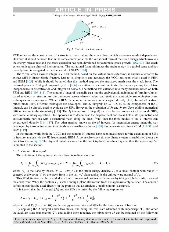
In the present work, both the VCCI and the contour M integral have been investigated for the calculation of SIFsin fracture analysis via the 3D isogeometric BEM. A point-wise crack tip coordinate system is established along thecrack front as in Fig. 3. The physical quantities are all in the crack tip local coordinate system thus the superscript ‘o’is omitted in the section.
5.1.1. Contour M integralThe definition of the Jk integral stems from two dimensions as:
Jk := limΓϵ→0
Γϵ
(Wδ jk − σi j ui,k)n j dΓ = limΓϵ→0
Γϵ
Pk j n j dΓ , k = 1, 2 (39)
where Pk j is the Eshelby tensor, W = 1/2σi jϵi j is the strain energy density. Γϵ is a small contour with radius Rcentered at the point ‘o’ on the crack front in the ‘xo–yo’ plane and n j is the unit outward normal of Γϵ .
This 2D definition can be extended to a three dimensional point-wise definition by taking a tubular surface aroundthe crack front. When the contour Γϵ is small enough, plane strain conditions are approximately satisfied. The contourdefinition can thus be used directly on the premise that a sufficiently small contour is assumed.
It is known that the J integral (J1) and the SIFs are linked by the following expression
J = G I + GII + GIII =1 − ν2
EK 2
I +1 − ν2
EK 2
II +1
2µK 2
III, (40)
where Gi and Ki (i = I, II, III) are the energy release rates and SIFs for the three modes of fracture.By applying the J integral under two states, one being the real state (denoted with superscript ‘1’), the other
the auxiliary state (superscript ‘2’), and adding them together, the mixed term M can be obtained by the following

X. Peng et al. / Comput. Methods Appl. Mech. Engrg. ( ) – 15
manipulation:
J (1+2)=
Γϵ
12(σ(1)i j + σ
(2)i j )(ϵ
(1)i j + ϵ
(2)i j )δ1 j − (σ
(1)i j + σ
(2)i j )
∂(u(1)i + u(2)i )
∂x1
n j dΓ . (41)
Rearranging the two state terms gives
J (1+2)= J (1) + J (2) + M (1,2) (42)
where
M (1,2)=
Γϵ
W (1,2)δ1 j − σ
(1)i j
∂u(2)i
∂x1− σ
(2)i j
∂u(1)i
∂x1
n j dΓ (43a)
W (1,2)= σ
(1)i j ϵ
(2)i j = σ
(2)i j ϵ
(1)i j . (43b)
Combined with Eq. (40), the following relationship can be obtained for the M integral,
M (1,2)=
2(1 − ν2)
E(K (1)
I K (2)I + K (1)
II K (2)II )+
1µ
K (1)III K (2)
III . (44)
The SIFs can then be extracted by making specific selections for state 2. For example, if the auxiliary mode is the puremode III asymptotic fields with K (2)
I = 0, K (2)II = 0, K (2)
III = 1 then, KIII in real state 1 can be found as
K (1)III = µM (1, mode III) (45)
K I and KII can be obtained in a similar fashion. In this work the first order asymptotic displacement and stresssolutions (see Appendix A) are selected as auxiliary fields.
5.1.2. Virtual crack closure integralIn the VCCI, the strain energy release rate is equal to the work done by closing the crack along its extension. The
modes of the strain energy release rate are given by
G I =1
2R
R
0σyy(x)[[u y(R − x)]]dx,
GII =1
2R
R
0σxy(x)[[ux (R − x)]]dx,
GIII =1
2R
R
0σyz(x)[[uz(R − x)]]dx,
(46)
where O P ′= R is the virtual crack advance. For the evaluation of [[u j (R − x)]] on P O , the point inversion algorithm
needs to be performed in order to find the parametric coordinates in the crack modeled by the NURBS surface [84].The domains of these integrals O P ′ and P O are discretized by a single linear element [120]. R is identical for all thesample points on the crack front. Then K I , KII and KIII can be computed according to Eq. (40).
5.2. Paris law
The Paris-based laws are typical empirical relation linking the increment in crack advance da occurring during dNcycles to the SIF amplitude, though empirically obtained coefficients C and m. The simplest expression of Paris lawreads:
da
dN= C(∆K )m . (47)
For mixed mode fracture, K is taken as the equivalent SIF Keq which is given as [7]:
Keq =
K 2
I + K 2II + (1 + ν)K 2
III . (48)

16 X. Peng et al. / Comput. Methods Appl. Mech. Engrg. ( ) –
Fig. 4. Crack surface updating for a growth step. The red rectangles denote the control points of NURBS curves. (a) The crack front curve C(ξ)is extracted from the original crack surface. The Greville Abscissae is used to obtain sample points (blue crosses). New position of those sample
points (green crosses) M ′j (ξ) is determined by ∆a j and θ j
c from the fracture law. (b) New front curve C′(ξ) is obtained by moving the controlpoints of C(ξ) iteratively until the criterion in the algorithm is met. (c) A new crack surface is obtained by linear interpolation between the twocurves C(ξ) and C′(ξ). (For interpretation of the references to color in this figure legend, the reader is referred to the web version of this article.)
It should be noted that the crack propagation velocity could be varied for the points along the front. In a singlepropagation step, the crack advance for each point is regularized by the user-specified maximum increment of crackadvance ∆amax,
∆ai= C(∆K i
eq)m ∆amax
C(∆K maxeq )
= ∆amax ∆K i
eq
∆K maxeq
m. (49)
The maximum hoop stress criterion is used to determine the direction of crack propagation. We assume, at each pointon the crack front, that the crack propagates in the direction θc such that the hoop stress is maximum. This is given bythe following expression [121]
θc = 2 arctan
−2(KII/K I )
1 +
1 + 8(KII/K I )2
. (50)
5.3. Crack surface updating algorithm
Crack propagation is realized geometrically by advancing the crack front so that the new crack front curve C′(ξ)
passes through the new positions of the sample points on the old crack front curve C(ξ) which is parametrized by theknot vector Ξ = ξ1, ξ2, . . . , ξn+p+1, n is the number of basis functions. We define the sample points on C(ξ) to beM j = C(ξ j ), j = 1, 2, . . . , N , and the set of points with new position to be M ′
j = C′(ξ j ) and we set N = n here.Note that each M ′
j is calculated via the fracture parameters K and ∆a introduced in the previous section. We adoptthe algorithm described in [96] to generate a new curve which passes through all the new sample points by updatingthe control points of the old curve through an iterative process. For t th iteration step, we define the error vector et as:
e j,t =−−−−→M j,t M ′
j , j = 1, 2, . . . , N . (51)
Note that when t = 0, e j,t =−−−−→M j,0 M ′
j =−−−→M j M ′
j = ∆a j which is the crack advance of the point on the crack front. If∥et∥ < tol, the iteration ceases and the new crack front curve is obtained (see Fig. 4).
To update the control points, we define a motion vector mt for the control points such that at the t th iteration step:
Pi,t = Pi,t−1 + mi,t , i = 1, 2, . . . , n, (52)
X. Peng et al. / Comput. Methods Appl. Mech. Engrg. ( ) – 17
with Pi,0 = Pi which are the control points of the old crack front C. The motion vector mt can be computed as:
mi,t =1N
Nj=1
fi j e j,t−1, t > 1, (53)
where fi j = fi (ξ j ) are the influence functions corresponding to each constraint M ′
j . We choose the influence functionsto be the NURBS basis functions which are used to describe the curve, i.e. fi (ξ) = Ri (ξ). The parameter coordinate ξ jof each M j should satisfy ξ j ∈ [ξi , ξi+p+1]. We use the Greville Abscissae to generate the sample points to make surethe influence functions associated with each M ′
j are linearly independent [96]. Finally, the error vector is calculatedin a recursive way:
e j,t = e j,t−1 −1N
Nk=1
ni=1
Ri j fikek,t−1, (54)
where Ri j = Ri (ξ j ). The details for updating the crack front is given in Algorithm 1. Once the new crack front curveis obtained, the new crack surfaces can be generated by lofting along the crack extension direction from the old curveto the new curve. The generated crack surfaces can be merged into the old crack surfaces with either a C0 joint or aC1 joint. In this work a C0 merging is adopted.
Algorithm 1 Crack front updating algorithm
Data: old crack front curve C(ξ); sample points M j ; new positions of sample points M ′
jResult: new crack front curve that passes through all M ′
jt = 0;tol = 1.e − 4;
e j,0 =−−−−→M j,0 M ′
j ; //the initial error vector
while ∥et∥ > tol dot = t + 1;mi,t =
1N
Nj=1 fi j e j,t−1; //the motion vector at t-th step
Pi,t = Pi,t−1 + mi,t ; //the new point on the crack front at t-th stepe j,t = e j,t−1 −
1N
Nk=1
ni=1 Ri j fikek,t−1; //the error vector at t-th step
end
6. Numerical examples
In this section, numerical examples are presented as follows: In the first two examples we study penny-shaped andelliptical static cracks. We conduct (a) detailed study of suggested integration schemes; (b) convergence analysis; (c)accuracy tests for SIF calculations. In the next two examples we demonstrate the application of the crack propagationalgorithm for fatigue crack growth simulation of an in-plane penny crack and inclined elliptical crack. The Young’smodulus E = 1000 and Poisson’s ratio ν = 0.3 for all cases. The relative error in the L2 norm of COD is computedas
eL2 =
S([[u]] − [[u ]]ext)([[u]] − [[u ]]ext)
TdSS[[u ]]ext[[u ]]
Text dS
, (55)
where the subscript ‘ext’ denotes the analytical solution of COD.
6.1. Penny-shaped crack
Suppose a penny-shaped crack is subjected to the remote tension σ0, i.e. t∞ = (0, 0, σ0). The radius of circle is a.The inclination angle is ϕ and circular angle θ is defined in the crack plane (Oxy) as in Fig. 5. The analytical solution

18 X. Peng et al. / Comput. Methods Appl. Mech. Engrg. ( ) –
Fig. 5. Geometry for penny-shaped crack (a = b) and elliptical crack (a = b).
for the SIFs read:
K I (ϕ) =2πσ0
√aπ cos2 ϕ,
KII(ϕ, θ) =4
π(2 − ν)σ0
√aπ cosϕ sinϕ cos θ,
KIII(ϕ, θ) =4(1 − ν)
π(2 − ν)σ0
√aπ cosϕ sinϕ sin θ.
(56)
In particular, when the crack plane is horizontal (ϕ = 0), the analytical normal displacement is given as:
uz(r, θ, 0) =2(1 − ν)σ0
πµ
a2 − r2, r 6 a. (57)
6.1.1. Singular integration testThe problem is modeled by COD equation (10), so that a single NURBS patch is necessary to represent the crack.
Fig. 6(a) illustrates the NURBS Surface which is composed of 4 elements and Fig. 6(b) is obtained by 1 time uniformmesh refinement based on (a). (c) and (d) present the knot lines in parametric space. For the sake of convenientdescription in the following context, we name the ξ direction as the angular direction of the disc and the η direction asthe radial direction and it can be observed that η = 1 represents the crack front (Fig. 6). The control points for (a) aregiven in Appendix B. It can be seen that the control points are coinciding at the pole of the disc. The collocation pointsare moved aside from the pole in order not to locate at the degenerated point. The NURBS basis functions associatedwith the pole, however, are enforced to be C0 through sharing the same degrees of freedom. The BIEs from thesemoved collocation points are merged into one equation.
We note that the COD solution only varies in the radial direction and is constant in the angular direction, thus 4elements are used in the angular direction. This will lead to high aspect ratio of each element with the refinement inthe radial direction. Fig. 9 compares the L2 norm error in COD for ϕ = 0. ‘ngp s’ denotes the number of Gauß pointsin the angular direction in each sub-triangle. By ‘original SST’, we mean a direct use of the method and by ‘improvedSST’, the SST with conformal and Sigmoidal transformation. It can be observed that
• when ngp s = 30, the errors of the original SST and improved SST are comparable. However, the error from theoriginal SST is non-uniformly distributed whilst the improved SST provides a more uniform error distribution;
• when ngp s = 18, the error from the original SST increases significantly (eL2 = 1.467716e−1), while the im-proved SST maintains the same accuracy as for ngp s = 30;
• the error is larger near the crack front. This is due to the crack tip singularity.
We conclude that the original SST requires more Gauß points for the same accuracy level as the improved SST. If wemove the knot (η = 0.875) next to the crack front in the radial direction closer to the crack front (η = 0.94) (the knotindicated by red solid line is moved to red dashed line in Fig. 8) and repeat the comparison of Fig. 10, we find that

X. Peng et al. / Comput. Methods Appl. Mech. Engrg. ( ) – 19
(a) Coarse mesh: the initial geometry for penny crack. (b) Finer mesh: the 1 time uniform refinement in parameterspace based on initial geometry.
(c) Parametric space for coarse mesh. (d) Parametric space for finer mesh.
Fig. 6. NURBS represented (p = q = 2) penny crack. Knot vectors for coarse mesh, the red rectangles are control points: angulardirection ξ = [0, 0, 0, 0.25, 0.25, 0.5, 0.5, 0.75, 0.75, 1, 1, 1], radial direction η = [0, 0, 0, 1, 1, 1]. For finer mesh:angular direction ξ =
[0, 0, 0, 0.125, 0.25, 0.25, 0.375, 0.5, 0.5, 0.625, 0.75, 0.75, 0.875, 1, 1, 1], radial direction η = [0, 0, 0, 0.5, 1, 1, 1] (For interpretation of thereferences to color in this figure legend, the reader is referred to the web version of this article.)
even for ngp s = 30, the original SST still gives error as large as for ngp s = 18 while the improved method gives anerror of eL2 = 1.755681e−2, which is lower than what was shown in Fig. 9. We can refer that, due to the crack tipsingularity, a refined mesh near the crack front should give a better accuracy in COD, but the original SST is sensitiveto the element distortion and gives diverged results. The improved SST presents a robust application for this kind ofmesh configuration.
6.1.2. Convergence testWe perform uniform mesh refinement in parametric space as shown in Fig. 6 until 5 times. We calculate the element
size as h =
Smaxe , where Smax
e denotes the maximum area of the elements. The convergence curves are plotted inFig. 12. For IGABEM, the default α is 0.5 for both quadratic and cubic NURBS basis functions. We also compareddiscontinuous quadratic Lagrange element BEM (LBEM) [44] where the collocation points are moved inside eachelement in order to fulfill the continuity requirement in BIEs. The mesh for LBEM is generated from the NURBS

20 X. Peng et al. / Comput. Methods Appl. Mech. Engrg. ( ) –
(a) Coarse mesh. (b) Finer mesh.
Fig. 7. Discontinuous quadratic Lagrange element discretizations for penny crack. Blue dots are element nodes (collocation points) (Forinterpretation of the references to color in this figure legend, the reader is referred to the web version of this article.)
Fig. 8. Original knot vectors: angular direction ξ = [0, 0, 0, 0.25, 0.25, 0.5, 0.5, 0.75, 0.75, 1, 1, 1], radial direction η = [0, 0, 0, 0.5, 0.75,0.875, 1, 1, 1]. After moving the red solid line to red dashed place, knot vectors: angular direction ξ = [0, 0, 0, 0.25, 0.25, 0.5, 0.5, 0.75, 0.75, 1, 1, 1], radial direction η = [0, 0, 0, 0.5, 0.75, 0.94, 1, 1, 1]. (For interpretation of the references to color in this figure legend, the reader is referredto the web version of this article.)
surface and then it will maintain the same topological element discretization as in IGABEM, see Fig. 7. It can beconcluded that
• degree elevation of NURBS basis functions improves accuracy. Yet, the order of convergence rate (ocr ) of therelative error in the L2 norm of COD keeps almost the same value (ocr = 1). The deteriorated ocr is due to thephysical singularity along the crack front.
• When the value of α becomes smaller (which means the moved collocation points are closer to their originalposition according to Eq. (23)), the accuracy is improved. However, further deterioration in convergence rate forα = 0.1 is observed (ocr = 0.81). One possible reason for this could be the near singularity is stronger in theneighbor elements when the moved collocation points get close to the element edge.
• The quadratic Lagrange basis gains an accuracy close to quadratic NURBS basis with α = 0.25. Whilst the NURBSbasis with α = 0.1 outperforms the Lagrange basis in terms of accuracy.

X. Peng et al. / Comput. Methods Appl. Mech. Engrg. ( ) – 21
(a) Original SST, ngp s = 30, eL2 = 3.344418e−2. (b) Improved SST, ngp s = 30, eL2 = 3.844282e−2.
(c) Original SST, ngp s = 18, eL2 = 1.467716e−1. (d) Improved SST, ngp s = 18, eL2 = 3.844282e−2.
Fig. 9. The relative error in the L2 norm of COD for the penny crack problem for parametric space associated with red solid line. ‘ngp s’ denotesthe number of Gauß points in angular direction in each sub-triangle (For interpretation of the references to color in this figure legend, the reader isreferred to the web version of this article.)
As is well known, uniform refinement is neither effective nor efficient to improve the accuracy for the crack problem.Thus five mesh configurations are designed, through keeping the number of elements in the angular direction whilethe mesh is uniformly refined by 2, 4, 6, 8 and 10 elements in the radial direction. The elements along the crack frontis then further gradely refined by consecutive knot insertion to reduce the error caused by the crack tip singularity(Fig. 11 shows meshes 1, 3 and 5). Fig. 13 presents the result from this graded mesh refinement along with all theresults from uniform refinement in parametric space in terms of degrees of freedom and all the results from IGABEMoutperforms LBEM in efficiency. It can be seen that the accuracy is improved almost by one order compared touniform refinement and the final estimate convergence rate is two times higher than for uniform refinement. Thisindicates the effectivity of IGABEM for fracture simulation.
6.1.3. Stress intensity factor testIn this subsection, the computation of SIFs is verified. Although, one of the advantages of the boundary element
method for infinite domains is the necessity to discretize only the inner boundary (crack surface), the industrialapplications are more concerned with problems in finite domains. Thus, instead of using the COD equation to modelthe penny-shaped crack in an infinite domain, we embed two overlapping crack surfaces in a cube with size L = 200asuch that we can compare the numerical SIFs with the analytical solution for infinite domain. Dual equations are usedfor this case.
Fig. 14 shows the path independence of the M integral and VCCI for mode I penny-shaped crack. Here ‘R’ denotesthe virtual crack advance in VCCI and the radius of the contour in M integral. It can be seen that when R/a is from0.02 to 0.08, both methods show path dependent behavior. For M integral, the error varies within 2%. When theradius of contour is small, K I converges to analytical value; while increasing R, since the stress field for the cracktip is influence by other tips in the crack front, plane strain condition is not satisfied properly, the method becomesinaccurate. For VCCI, the error varies within 6% and generally a small virtual crack advance is needed. However, ifR is too small, difficulty in numerical evaluation of stress and COD close to crack front will arise which lead to the

22 X. Peng et al. / Comput. Methods Appl. Mech. Engrg. ( ) –
(a) Original SST, ngp s = 30, eL2 = 8.138911e−1. (b) Improved SST, ngp s = 30, eL2 = 1.755681e−2.
(c) Original SST, ngp s = 18, eL2 = 7.110011e−1. (d) improved SST, ngp s = 18, eL2 = 1.755679e−2.
Fig. 10. The relative error in the L2 norm of COD for the penny crack problem for parametric space associated with red dashed line (Forinterpretation of the references to color in this figure legend, the reader is referred to the web version of this article.)
Fig. 11. NURBS (p = q = 2) represented crack surface meshes with 2, 6, and 10 uniform refinement in the radial direction, followed by gradedrefinement (with black edges) close to crack front. The blue dots are collocation points.
inaccuracy of K I . From the figure we can also refer that M integral presents a smaller reduction in error than VCCI.Therefore the M integral is recommended to use for crack growth simulation by IGABEM.
Fig. 15 compares the SIFs obtained from M integral with R = 0.02a and VCCI with R = 0.04a for the mixedmode penny-shaped crack with inclination angle ϕ = π/6. It is seen that both methods agree well with the analyticalsolution. KIII from M integral shows deviation near θ = π/2 and 3π/2. Table 1 presents the error at θ = 0, π/4 andπ/2. It can be observed that the error of K I and KII is within 1% by both methods, while within 7% for KIII by Mintegral. We can conclude that the IGABEM can provide accurate SIFs, and the numerical SIFs along crack front isquite smooth, although with only 4 elements in angular direction and without any smoothness operation. This givesthe premise for a stable evolution for the crack growth simulation.
An inclined penny crack (ϕ = π/4) centered at a cylindrical bar is analyzed by IGABEM, the geometric size andboundary condition can be found in the work by Mi and Aliabadi [44]. In that work, the discontinuous Lagrange

X. Peng et al. / Comput. Methods Appl. Mech. Engrg. ( ) – 23
Fig. 12. The relative error in the L2 norm of COD for penny-shaped crack. The default offset α = 0.5.
Fig. 13. The relative error in the L2 norm of COD for penny-shaped crack. The default offset α = 0.5.
Table 1Error of SIFs for penny-shaped crack with ϕ = π/6.
K I KII KIIIVCCI M integral VCCI M integral VCCI M integral
θ = 0 2.874e−3 4.311e−3 7.133e−3 2.008e−3 2.898e−8 5.221e−9θ = π/4 2.874e−3 4.311e−3 7.167e−3 1.983e−3 1.591e−4 6.243e−2θ = π/2 2.874e−3 4.311e−3 1.622e−8 1.228e−8 2.010e−4 1.894e−2
elements are used to discretize the crack surfaces. Fig. 16 compares the SIFs by IGABEM and Lagrange BEMfrom [44]. It should be noted that for the presented result by Lagrange basis in Fig. 16, 8 elements are used in theangular direction while for IGABEM, mesh 1 in Fig. 11 (4 elements in angular direction) is used. It can be observedthat the discontinuous Lagrange BEM shows fluctuation in SIFs. While the SIFs by IGABEM is smoother. Furthermesh refinement needs to be performed such that the crack front can be described more accurately in order to reducethe oscillation for Lagrange BEM [44]. While in IGABEM, the crack shape is exactly represented and the local crack

24 X. Peng et al. / Comput. Methods Appl. Mech. Engrg. ( ) –
Fig. 14. Path independence verification for VCCI and M integral. Here ‘R’ denotes the virtual crack advance in VCCI and the radius of the contourin M integral.
Fig. 15. Stress intensity factors for penny crack with ϕ = π/6.
Fig. 16. Stress intensity factors for penny crack with ϕ = π/4. LBEM denotes the discontinuous Lagrange basis BEM.
tip coordinate system is well defined thanks to the smoothness in geometry. This will lead to more accurate evaluationin fracture parameters with less elements. This example illustrates the efficiency of IGABEM for fracture simulation.

X. Peng et al. / Comput. Methods Appl. Mech. Engrg. ( ) – 25
(a) Original SST, ngp s = 18, eL2 = 4.603473e−1. (b) Improved SST, ngp s = 18, eL2 = 3.798002e−2.
Fig. 17. Error in crack opening displacement for elliptical crack. Knot vectors: angular direction ξ = [0, 0, 0, 0.25, 0.25, 0.5, 0.5, 0.75, 0.75,1, 1, 1], radial direction η = [0, 0, 0, 0.5, 0.75, 0.875, 1, 1, 1].
6.2. Elliptical crack
Suppose an elliptical crack is subjected to the remote tensile loading σ0 in the normal direction, i.e. t∞ = (0, 0, σ0).The semi-major axis is a, semi-minor axis b. The initial NURBS data can be found in Appendix B. The inclinationangle is ϕ and the elliptical angle θ is defined in the crack plane as in Fig. 5. The analytical SIFs read:
K I (ϕ, θ) =σ0
2(1 + cos 2ϕ)
√bπ f (θ)
E(k),
KII(ϕ, θ) =σ0
2sin 2ϕ
√bπk2(b/a) cos θ
f (θ)B(k),
KIII(ϕ, θ) =σ0
2sin 2ϕ
√bπk2(1 − ν) sin θ
f (θ)B(k),
k2= 1 −
b2
a2 ,
f (θ) =
sin2 θ +
b2
a2 cos2 θ1/4
,
B(k) = (k2− ν)E(k)+ ν
b2
a2 K (k),
(58)
where K (k) and E(k) are elliptic integrals of the first kind and second kind, respectively:
K (k) =
π/2
0
11 − k2 sin2 θ
dθ,
E(k) =
π/2
0
1 − k2 sin2 θdθ.
(59)
In particular, when ϕ = 0, the displacement in the normal direction to the crack reads:
uz(x, y, 0) =2(1 − ν)σ0
µ
b
E(k)
1 −
x2
a2 −y2
b2 . (60)
The difference of the elliptical crack and penny crack is that the mode I SIF is not a constant, due to the variationof the curvature along the crack front. The problem is modeled by COD equation (10) and mesh configuration andcollocation strategy is analogous to the case of the penny-shaped crack. For elliptical cracks, the elements have highaspect ratios as well as non-orthogonal basis vectors. Fig. 17 shows that original SST presents erroneous result with18 Gauß points in angular direction. While the improved SST gives a reasonable COD and error distribution.
For the convergence study, we first give the result of uniform refinement in parametric space in Fig. 19 as well as theresult from LBEM with discontinuous Lagrange basis. Then the same graded mesh configurations for elliptical crackare generated as done for penny crack as in Fig. 18. Fig. 20 compares the result between uniform mesh and graded

26 X. Peng et al. / Comput. Methods Appl. Mech. Engrg. ( ) –
Fig. 18. The NURBS (p = q = 2) represented crack surface meshes with 1, 5, and 9 uniformed refinement in radial direction, followed by gradedrefined elements (with black edges) close to crack front. The blue dots are collocation points.
Fig. 19. L2 norm error of COD for elliptical crack.
Fig. 20. L2 norm error of COD for elliptical crack.
mesh. The convergence feature is almost the same as that of penny crack. And we can conclude that the IGABEMalso suits well for modeling elliptical crack.
For the test of SIFs computation, we put two overlapping crack surfaces in a cube with size L = 200a such that wecould compare the numerical SIFs with the analytical solution for infinite domain. Dual equations are used. Fig. 21compares the SIFs obtained from M integral with R = 0.02b and VCCI with R = 0.02b for the mixed mode ellipticalcrack with inclination angle ϕ = π/6. Table 2 presents the error at θ = 0 and π/2 for the SIF in three modes. It canbe seen that the error for all the SIFs is within 7%. And the SIFs along the crack front is smooth. We note that the SIFs

X. Peng et al. / Comput. Methods Appl. Mech. Engrg. ( ) – 27
Fig. 21. Stress intensity factors for elliptical crack with ϕ = π/6.
Table 2Relative error of SIFs for elliptical crack with ϕ = π/6.
K I KII KIIIVCCI M integral VCCI M integral VCCI M integral
θ = 0 4.564e−2 1.534e−2 4.138e−2 1.279e−2 1.226e−7 2.174e−7θ = π/2 8.284e−3 2.214e−2 6.936e−8 5.152e−8 6.882e−3 5.959e−2
accuracy for the elliptical crack is worse than for the penny crack, which is due to the variation of the crack curvaturealong the crack front. Since a fixed value of R is used, the singularity at the sample points near the semi-major andsemi-minor axes would be different, which leads to inaccuracies in the SIFs evaluation [122]. More suitable way toestimate the SIFs for elliptical crack would be one of the future work.
6.3. Fatigue crack growth
6.3.1. In-plane penny crack growthIn this section, the crack surface updating algorithm is tested using the Paris law as a crack growth law. We first
check the crack growth of the horizontal penny crack under uniform tension from Section 6.1.3. The fatigue parametersm = 2.1 and the specified ∆amax = 0.2a. We propagate 10 steps and make a comparison with the exact result and theresult from the XFEM + level set method [123] (Fig. 22(a) and (b)). It can be observed that the crack front for eachstep agrees well with exact solution by IGABEM, while the crack front deviates gradually from the exact solutionwith XFEM + level set method, due to the fact that the level set method is restricted in describing the crack frontexactly and this inaccuracy accumulates at each step. We then compute the crack propagation for m = 5, and theresult is presented in Fig. 22(c). We find that the numerical crack front still agrees well with the exact front, althoughthe high index amplifies the error in crack growth rate. In order to quantitatively scale the error, we define the relativeerror of the numerical crack front Γnum to the exact front Γext as:
E f (x) =|Γnum(x)− Γext(x)|
∆a,
error =
Γ E f (x)dΓext(x)
Γ dΓext(x).
(61)
Fig. 23 gives the relative error of the numerical crack front by IGABEM. It can be seen that the error accumulates ina slow speed and the difference of m = 5 and m = 2.1 is small, although the error for m = 5 is larger than m = 2.1as expected. This test shows the proposed crack propagation scheme has the ability to grow cracks in a stable andaccurate manner, thanks to the smoothness in the stress field and SIFs solution and to the exact representation of thegeometry of the crack during the crack growth.

28 X. Peng et al. / Comput. Methods Appl. Mech. Engrg. ( ) –
(a) IGABEM, m = 2.1. (b) XFEM/FMM, m = 2.1, Sukumar et al. 2003.
(c) IGABEM, m = 5.
Fig. 22. Fatigue crack growth of the first 10 steps of a penny crack.
Fig. 23. Relative error of the crack front (Eq. (61)) for each crack growth step by IGABEM.
6.3.2. Inclined elliptical crack growth
Finally, we simulate crack growth for an elliptical crack with inclination angle ϕ = π/6 modeled by the dualequations in a finite domain taken from Section 6.2. Fig. 24 illustrates the 2nd, 5th and 10th of the propagation step.

X. Peng et al. / Comput. Methods Appl. Mech. Engrg. ( ) – 29
(a) Step 2. (b) Step 5. (c) Step 10.
Fig. 24. Fatigue crack growth simulation of an elliptical crack.
7. Conclusions
Starting from computer aided design (CAD) NURBS data, as input, we formulated, implemented and described indetail a numerical method to simulate crack propagation in 3D, directly from the NURBS representation of the domainand which requires no mesh generation or regeneration as the cracks propagate. We investigated the advantages anddrawbacks of the approach, and proposed a number of improvements to the naıve approach which makes the methodamenable to realistic 3D damage tolerance assessment problems encountered in industry.
The key idea is to use the same NURBS basis functions have been used for the discretization of the geometry andcrack and for the approximation of the displacement and traction fields. We used the singularity subtraction technique(SST) proposed in [83] for the treatment of (hyper-)singular integrals in the boundary element method. We extendedthe improved SST [87] to quadrilateral elements such that it can be applied to tensor-product NURBS basis functions.We used both the crack opening displacement (COD) form and the dual equations of IGABEM to model the crack.We tested two methods to extract SIFs: the contour-based M integral and the virtual crack closure approach. Wealso proposed and verified an algorithm to propagate the NURBS-represented crack surface. The conclusions andhighlights of this work include:
• The proposed singular integration scheme preserves the quadratic accuracy for highly distorted elements whichcommonly arise in isogeometric analysis. This enables a robust implementation of IGABEM;
• Through graded mesh refinement in the direction where the crack tip singularity varies, the convergence rate canbe improved by a factor of 2 and the accuracy improved by one order, compared to uniform refinement. This showsthe promise of IGABEM for fracture problem;
• A local crack tip system is setup naturally and uniquely thanks to the NURBS representation of the crack surface.Combining this approach with the high-order continuity in stress provided by the NURBS-based BEM, the SIFscomputed along the crack front are smooth and accurate;
• The proposed algorithm for crack propagation is stable, even for high exponent values in the Paris law, due to thesmoothness in the crack front geometry and the accuracy of the SIFs.
The use of CAD geometry directly for fracture simulation provides benefits. Nevertheless, specific difficulties tomodel surface cracks must be overcome. Introducing and growing these edge-discontinuities into a NURBS patch atan arbitrary position requires particular care, due to the higher order continuity of the basis functions. Future workwill focus on the propagation of surface cracks. Dealing with multi-patch geometries and handling crack propagationthrough patch interfaces is another important avenue of investigation to extend and complement the method proposedhere. Meanwhile, the fast solution as proposed in [42] is being implemented to accelerate the simulations.
Acknowledgments
The first and last authors would like to acknowledge the financial support of the Framework Programme 7 InitialTraining Network Funding under grant number 289361 ‘Integrating Numerical Simulation and Geometric DesignTechnology’. S.P.A. Bordas also thanks partial funding for his time provided by the UK Engineering and PhysicalScience Research Council (EPSRC) under grant EP/G069352/1 Advanced discretization strategies for ‘atomistic’nano CMOS simulation; the EPSRC under grant EP/G042705/1 ‘Increased Reliability for Industrially RelevantAutomatic Crack Growth Simulation with the eXtended Finite Element Method’ and the European Research CouncilStarting Independent Research Grant (ERC Stg grant agreement No. 279578) entitled ‘Towards real time multiscale

30 X. Peng et al. / Comput. Methods Appl. Mech. Engrg. ( ) –
simulation of cutting in non-linear materials with applications to surgical simulation and computer guided surgery’.E. Atroshchenko was partially supported by Fondecyt grant number 11130259 entitled ‘Boundary element modelingof crack propagation in micropolar materials’.
Appendix A. Auxiliary displacement and stress fields in M integral
The auxiliary stress field σ (2)i j and displacement field u(2)j are given as:
σxx =K (2)
I√
2πrcos
θ
2
1 − sin
θ
2sin
3θ2
−
K (2)II
√2πr
sinθ
2
2 + cos
θ
2cos
3θ2
σyy =
K (2)I
√2πr
cosθ
2
1 + sin
θ
2sin
3θ2
+
K (2)II
√2πr
sinθ
2cos
θ
2cos
3θ2,
τxy =K (2)
I√
2πrsin
θ
2cos
θ
2cos
3θ2
+K (2)
II√
2πrcos
θ
2
1 − sin
θ
2sin
3θ2
,
τyz =K (2)
III√
2πrcos
θ
2,
τzx = −K (2)
III√
2πrsin
θ
2,
τzz = ν(σxx + σyy),
ux =K I
2µ
r
2πcos
θ
2
κ − 1 + 2 sin2 θ
2
+(1 + ν)KII
E
r
2πsin
θ
2
κ + 1 + 2 cos2 θ
2
,
u y =K I
2µ
r
2πsin
θ
2
κ + 1 − 2 cos2 θ
2
+(1 + ν)KII
E
r
2πcos
θ
2
1 − κ + 2 sin2 θ
2
,
uz =2KIII
µ
r
2πsin
θ
2
(62)
where (r, θ) are the crack tip polar coordinates and µ =E
2(1+ν), κ = 3 − 4ν.
The auxiliary strain field can be obtained by differentiating u j with respect to the physical coordinate.
Appendix B. Geometry data
See Tables 3 and 4.
Table 3Control points for NURBS-represented penny crack.The knot vectors are: angular direction ξ =
[0, 0, 0, 0.25, 0.25, 0.5, 0.5, 0.75, 0.75, 1, 1, 1], radialdirection η = [0, 0, 0, 1, 1, 1].
i j Pi, j wi, j
0 0 (0.0, 0.0) 1.01 0 (0.0, 0.0) 0.7071062 0 (0.0, 0.0) 1.03 0 (0.0, 0.0) 0.7071064 0 (0.0, 0.0) 1.05 0 (0.0, 0.0) 0.7071066 0 (0.0, 0.0) 1.07 0 (0.0, 0.0) 0.707106
(continued on next page)
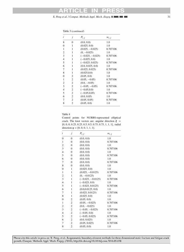
X. Peng et al. / Comput. Methods Appl. Mech. Engrg. ( ) – 31
Table 3 (continued)
i j Pi, j wi, j
8 0 (0.0, 0.0) 1.00 1 (0.025, 0.0) 1.01 1 (0.025, −0.025) 0.7071062 1 (0, −0.025) 1.03 1 (−0.025, −0.025) 0.7071064 1 (−0.025, 0.0) 1.05 1 (−0.025, 0.025) 0.7071066 1 (0.0, 0.025, 0.0) 1.07 1 (0.025, 0.025) 0.7071068 1 (0.025,0.0) 1.00 2 (0.05, 0.0) 1.01 2 (0.05, −0.05) 0.7071062 2 (0.0, −0.05) 1.03 2 (−0.05, −0.05) 0.7071064 2 (−0.05,0.0) 1.05 2 (−0.05,0.05) 0.7071066 2 (0.0, 0.05) 1.07 2 (0.05, 0.05) 0.7071068 2 (0.05, 0.0) 1.0
Table 4Control points for NURBS-represented ellipticalcrack. The knot vectors are: angular direction ξ =
[0, 0, 0, 0.25, 0.25, 0.5, 0.5, 0.75, 0.75, 1, 1, 1], radialdirection η = [0, 0, 0, 1, 1, 1].
i j Pi, j wi, j
0 0 (0.0, 0.0) 1.01 0 (0.0, 0.0) 0.7071062 0 (0.0, 0.0) 1.03 0 (0.0, 0.0) 0.7071064 0 (0.0, 0.0) 1.05 0 (0.0, 0.0) 0.7071066 0 (0.0, 0.0) 1.07 0 (0.0, 0.0) 0.7071068 0 (0.0, 0.0) 1.00 1 (0.025, 0.0) 1.01 1 (0.025, −0.0125) 0.7071062 1 (0, −0.0125) 1.03 1 (−0.025, −0.0125) 0.7071064 1 (−0.025, 0.0) 1.05 1 (−0.025, 0.0125) 0.7071066 1 (0.0,0.0125, 0.0) 1.07 1 (0.025, 0.0125) 0.7071068 1 (0.025, 0.0) 1.00 2 (0.05, 0.0) 1.01 2 (0.05, −0.025) 0.7071062 2 (0.0, −0.025) 1.03 2 (−0.05, −0.025) 0.7071064 2 (−0.05, 0.0) 1.05 2 (−0.05, 0.025) 0.7071066 2 (0.0, 0.025) 1.07 2 (0.05, 0.025) 0.7071068 2 (0.05, 0.0) 1.0

32 X. Peng et al. / Comput. Methods Appl. Mech. Engrg. ( ) –
References
[1] T. Rabczuk, S. Bordas, G. Zi, On three-dimensional modelling of crack growth using partition of unity methods, Comput. Struct. 88 (23–24)(2010) 1391–1411.
[2] Roshdy S. Barsoum, Further application of quadratic isoparametric finite elements to linear fracture mechanics of plate bending and generalshells, Int. J. Fract. 11 (1) (1975) 167–169.
[3] L.F. Martha, P.A. Wawrzynek, A.R. Ingraffea, Arbitrary crack representation using solid modeling, Eng. Comput. 9 (2) (1993) 63–82.[4] V. Chiaruttini, V. Riolo, F. Feyel, Advanced remeshing techniques for complex 3D crack propagation, in: ICF13, 2013.[5] A.R. Khoei, M. Eghbalian, H. Moslemi, H. Azadi, Crack growth modeling via 3D automatic adaptive mesh refinement based on modified-
SPR technique, Appl. Math. Model. 37 (1) (2013) 357–383.[6] M. Schollmann, M. Fulland, H.A. Richard, Development of a new software for adaptive crack growth simulations in 3D structures, Eng.
Fract. Mech. 70 (2) (2003) 249–268.[7] A.R. Maligno, S. Rajaratnam, S.B. Leen, E.J. Williams, A three-dimensional (3D) numerical study of fatigue crack growth using remeshing
techniques, Eng. Fract. Mech. 77 (1) (2010) 94–111.[8] B.J. Carter, P.A. Wawrzynek, A.R. Ingraffea, Automated 3-D crack growth simulation, Internat. J. Numer. Methods Engrg. 47 (1–3) (2000)
229–253.[9] R. Branco, F.V. Antunes, J.D. Costa, A review on 3D-FE adaptive remeshing techniques for crack growth modelling, Eng. Fract. Mech. 141
(2015) 170–195.[10] J.F. Remacle, V. Bertrand, C. Geuzaine, A two-level multithreaded delaunay kernel, Procedia Eng. 124 (2015) 6–17.[11] J. Pellerin, B. Levy, G. Caumon, A. Botella, Automatic surface remeshing of 3D structural models at specified resolution: A method based
on Voronoi diagrams, Comput. Geosci. 62 (2014) 103–116.[12] J.M. Melenk, I. Babuska, The partition of unity finite element method: Basic theory and applications, Comput. Methods Appl. Mech. Engrg.
139 (1–4) (1996) 289–314.[13] N. Moes, J. Dolbow, T. Belytschko, A finite element method for crack growth without remeshing, Internat. J. Numer. Methods Engrg. 46 (1)
(1999) 131–150.[14] C.A. Duarte, I. Babuska, J.T. Oden, Generalized finite element methods for three-dimensional structural mechanics problems, Computers &
Structures 77 (2) (2000) 215–232.[15] T. Strouboulis, K. Copps, I. Babuska, The generalized finite element method, Comput. Methods Appl. Mech. Engrg. 190 (32–33) (2001)
4081–4193.[16] G. Strang, G. Fix, An Analysis of the Finite Element Method, second ed., Wellesley-Cambridge, 2008.[17] M. Fleming, Y.A. Chu, B. Moran, T. Belytschko, enriched element-free Galerkin methods for crack tip fields, Internat. J. Numer. Methods
Engrg. 40 (8) (1997) 1483–1504.[18] V.P. Nguyen, T. Rabczuk, S. Bordas, M. Duflot, Meshless methods: A review and computer implementation aspects, Math. Comput.
Simulation 79 (3) (2008) 763–813.[19] J.J. Rodenas, O.A. Gonzalez-Estrada, J.E. Tarancon, F.J. Fuenmayor, A recovery-type error estimator for the extended finite element method
based on singular + smooth stress field splitting, Internat. J. Numer. Methods Engrg. 76 (4) (2008) 545–571.[20] M. Duflot, S.P.A. Bordas, A posteriori error estimation for extended finite elements by an extended global recovery, Internat. J. Numer.
Methods Engrg. 76 (8) (2008) 1123–1138.[21] S.P.A. Bordas, M. Duflot, Derivative recovery and a posteriori error estimate for extended finite elements, Comput. Methods Appl. Mech.
Engrg. 196 (35–36) (2007) 3381–3399.[22] S. Natarajan, S.P.A. Bordas, D.R. Mahapatra, Numerical integration over arbitrary polygonal domains based on Schwarz-Christoffel
conformal mapping, Internat. J. Numer. Methods Engrg. 80 (1) (2009) 103–134.[23] G. Ventura, R. Gracie, T. Belytschko, Fast integration and weight function blending in the extended finite element method, Internat. J. Numer.
Methods Engrg. 77 (1) (2009) 1–29.[24] R. Gracie, H. Wang, T. Belytschko, Blending in the extended finite element method by discontinuous Galerkin and assumed strain methods,
Internat. J. Numer. Methods Engrg. 74 (11) (2008) 1645–1669.[25] A. Menk, S.P.A. Bordas, A robust preconditioning technique for the extended finite element method, Internat. J. Numer. Methods Engrg. 85
(13) (2011) 1609–1632.[26] V. Gupta, C.A. Duarte, I. Babuska, U. Banerjee, Stable GFEM (SGFEM): Improved conditioning and accuracy of GFEM/XFEM for three-
dimensional fracture mechanics, Comput. Methods Appl. Mech. Engrg. 289 (2015) 355–386.[27] K. Agathos, E. Chatzi, S.P.A. Bordas, D. Talaslidis, A well-conditioned and optimally convergent XFEM for 3D linear elastic fracture,
Internat. J. Numer. Methods Engrg. 105 (9) (2015) 643–677.[28] N. Sukumar, N. Moes, B. Moran, T. Belytschko, Extended finite element method for three-dimensional crack modelling, Internat. J. Numer.
Methods Engrg. 48 (11) (2000) 1549–1570.[29] N. Sukumar, D.L. Chopp, E. Bechet, N. Moes, Three-dimensional non-planar crack growth by a coupled extended finite element and fast
marching method, Internat. J. Numer. Methods Engrg. 76 (5) (2008) 727–748.[30] A. Gravouil, N. Moes, T. Belytschko, Non-planar 3D crack growth by the extended finite element and level sets-Part II: Level set update,
Internat. J. Numer. Methods Engrg. 53 (11) (2002) 2569–2586.[31] N. Moes, A. Gravouil, T. Belytschko, Non-planar 3D crack growth by the extended finite element and level sets-Part I: Mechanical model,
Internat. J. Numer. Methods Engrg. 53 (11) (2002) 2549–2568.[32] S. Bordas, B. Moran, Enriched finite elements and level sets for damage tolerance assessment of complex structures, Eng. Fract. Mech. 73
(9) (2006) 1176–1201.[33] E. Wyart, M. Duflot, D. Coulon, P. Martiny, T. Pardoen, J.-F. Remacle, F. Lani, Substructuring FE–XFE approaches applied to three-
dimensional crack propagation, J. Comput. Appl. Math. 215 (2) (2008) 626–638.

X. Peng et al. / Comput. Methods Appl. Mech. Engrg. ( ) – 33
[34] P. Krysl, T. Belytschko, The element free Galerkin method for dynamic propagation of arbitrary 3-D cracks, Internat. J. Numer. MethodsEngrg. 44 (6) (1999) 767–800.
[35] G. Ventura, J.X. Xu, T. Belytschko, A vector level set method and new discontinuity approximations for crack growth by EFG, Internat. J.Numer. Methods Engrg. 54 (6) (2002) 923–944.
[36] S.P.A. Bordas, T. Rabczuk, G. Zi, Three-dimensional crack initiation, propagation, branching and junction in non-linear materials by anextended meshfree method without asymptotic enrichment, Eng. Fract. Mech. 75 (5) (2008) 943–960.
[37] T. Rabczuk, G. Zi, S. Bordas, H. Nguyen-Xuan, A simple and robust three-dimensional cracking-particle method without enrichment,Comput. Methods Appl. Mech. Engrg. 199 (37–40) (2010) 2437–2455.
[38] H. Hong, J. Chen, Derivations of integral equations of elasticity, J. Eng. Mech. 114 (6) (1988) 1028–1044.[39] J.T. Chen, H.K. Hong, Review of dual boundary element methods with emphasis on hypersingular integrals and divergent series, Appl.
Mech. Rev. 52 (1) (1999) 17–33.[40] T.J. Rudolphi, The use of simple solutions in the regularization of hypersingular boundary integral equations, Math. Comput. Modelling 15
(3–5) (1991) 269–278.[41] Y. Liu, T.J. Rudolphi, Some identities for fundamental solutions and their applications to weakly-singular boundary element formulations,
Eng. Anal. Bound. Elem. 8 (6) (1991) 301–311.[42] B. Marussig, J. Zechner, G. Beer, T.P. Fries, Fast isogeometric boundary element method based on independent field approximation, Comput.
Methods Appl. Mech. Engrg. 284 (2015) 458–488.[43] A. Portela, M.H. Aliabadi, D.P. Rooke, The dual boundary element method: Effective implementation for crack problems, Internat. J. Numer.
Methods Engrg. 33 (6) (1992) 1269–1287.[44] Y. Mi, M.H. Aliabadi, Dual boundary element method for three-dimensional fracture mechanics analysis, Engineering Analysis with
Boundary Elements 10 (2) (1992) 161–171.[45] A.P. Cisilino, M.H. Aliabadi, Dual boundary element assessment of three-dimensional fatigue crack growth, Engineering Analysis with
Boundary Elements 28 (9) (2004) 1157–1173.[46] A.P. Cisilino, M.H. Aliabadi, Three-dimensional boundary element analysis of fatigue crack growth in linear and non-linear fracture
problems, Eng. Fract. Mech. 63 (6) (1999) 713–733.[47] V. Leitao, M.H. Aliabadi, D.P. Rooke, The dual boundary element formulation for elastoplastic fracture mechanics, Internat. J. Numer.
Methods Engrg. 38 (2) (1995) 315–333.[48] P. Fedelinski, M.H. Aliabadi, D.P. Rooke, The dual boundary element method in dynamic fracture mechanics, Engineering Analysis with
Boundary Elements 12 (3) (1993) 203–210.[49] S.C. Mellings, J.M.W. Baynham, Automatic fatigue crack growth, in: ASME 2009 Pressure Vessels and Piping Conference, American
Society of Mechanical Engineers, 2009, pp. 1513–1523.[50] S. Li, M.E. Mear, L. Xiao, Symmetric weak-form integral equation method for three-dimensional fracture analysis, Comput. Methods Appl.
Mech. Engrg. 151 (3–4) (1998) 435–459.[51] A. Frangi, Fracture propagation in 3D by the symmetric Galerkin boundary element method, International Journal of Fracture 116 (4) (2002)
313–330.[52] A. Frangi, G. Novati, R. Springhetti, M. Rovizzi, 3D fracture analysis by the symmetric Galerkin BEM, Comput. Mech. 28 (3–4) (2002)
220–232.[53] G.P. Nikishkov, J.H. Park, S.N. Atluri, SGBEM-FEM alternating method for analyzing 3D non-planar cracks and their growth in structural
components, Comput. Model. Eng. Sci. 2 (3) (2001) 401–422.[54] A. Frangi, G. Novati, BEM–FEM coupling for 3D fracture mechanics applications, Comput. Mech. 32 (4–6) (2003) 415–422.[55] C. Song, J.P. Wolf, The scaled boundary finite-element method—alias consistent infinitesimal finite-element cell method—for
elastodynamics, Comput. Methods Appl. Mech. Engrg. 147 (3–4) (1997) 329–355.[56] S. Natarajan, J. Wang, C. Song, C. Birk, Isogeometric analysis enhanced by the scaled boundary finite element method, Comput. Methods
Appl. Mech. Engrg. 283 (2015) 733–762.[57] T.J.R. Hughes, J.A. Cottrell, Y. Bazilevs, Isogeometric analysis: CAD, finite elements, NURBS, exact geometry and mesh refinement,
Comput. Methods Appl. Mech. Engrg. 194 (39–41) (2005) 4135–4195.[58] E. De Luycker, D.J. Benson, T. Belytschko, Y. Bazilevs, M.C. Hsu, X-FEM in isogeometric analysis for linear fracture mechanics, Internat.
J. Numer. Methods Engrg. 87 (6) (2011) 541–565.[59] S. Ghorashi, N. Valizadeh, S. Mohammadi, Extended isogeometric analysis for simulation of stationary and propagating cracks, Internat. J.
Numer. Methods Engrg. 89 (9) (2012) 1069–1101.[60] V.P. Nguyen, C. Anitescu, S.P.A. Bordas, T. Rabczuk, Isogeometric analysis: An overview and computer implementation aspects, Math.
Comput. Simulation 117 (2015) 89–116.[61] N. Nguyen-Thanh, N. Valizadeh, M.N. Nguyen, H. Nguyen-Xuan, X. Zhuang, P. Areias, G. Zi, Y. Bazilevs, L. De Lorenzis, T. Rabczuk, An
extended isogeometric thin shell analysis based on Kirchhoff–Love theory, Comput. Methods Appl. Mech. Engrg. 284 (2015) 265–291.[62] R.N. Simpson, S.P.A. Bordas, J. Trevelyan, T. Rabczuk, A two-dimensional isogeometric boundary element method for elastostatic analysis,
Comput. Methods Appl. Mech. Engrg. 209–212 (0) (2012) 87–100.[63] H. Lian, R.N. Simpson, S.P.A. Bordas, Stress analysis without meshing: isogeometric boundary-element method, Proc. Inst. Civil Eng. -
Engrg. Comput. Mech. 166 (2) (2013) 88–99.[64] M.A. Scott, R.N. Simpson, J.A. Evans, S. Lipton, S.P.A. Bordas, T.J.R. Hughes, T.W. Sederberg, Isogeometric boundary element analysis
using unstructured T-splines, Comput. Methods Appl. Mech. Engrg. 254 (0) (2013) 197–221.[65] K. Li, X. Qian, Isogeometric analysis and shape optimization via boundary integral, Comput.-Aided Des. 43 (11) (2011) 1427–1437.[66] K.V. Kostas, A.I. Ginnis, C.G. Politis, P.D. Kaklis, Ship-hull shape optimization with a T-spline based BEM–isogeometric solver, Comput.
Methods Appl. Mech. Engrg. 284 (2015) 611–622.

34 X. Peng et al. / Comput. Methods Appl. Mech. Engrg. ( ) –
[67] H. Lian, P. Kerfriden, S.P.A. Bordas, Implementation of regularized isogeometric boundary element methods for gradient-based shapeoptimization in two-dimensional linear elasticity, Internat. J. Numer. Methods Engrg. 106 (12) (2016) 972–1017.
[68] R.N. Simpson, M.A. Scott, M. Taus, D.C. Thomas, H. Lian, Acoustic isogeometric boundary element analysis, Comput. Methods Appl.Mech. Engrg. (2013) page accepted.
[69] J. Gu, J. Zhang, G. Li, Isogeometric analysis in BIE for 3-D potential problem, Engineering Analysis with Boundary Elements 36 (5) (2012)858–865.
[70] C. Politis, A.I. Ginnis, P.D. Kaklis, K. Belibassakis, C. Feurer, An isogeometric BEM for exterior potential-flow problems in the plane,in: 2009 SIAM/ACM Joint Conference on Geometric and Physical Modeling, SPM’09, ACM, New York, NY, USA, 2009, pp. 349–354.
[71] A.I. Ginnis, K.V. Kostas, C.G. Politis, P.D. Kaklis, K.A. Belibassakis, Th.P. Gerostathis, M.A. Scott, T.J.R. Hughes, Isogeometric boundary-element analysis for the wave-resistance problem using T-splines, Comput. Methods Appl. Mech. Engrg. 279 (2014) 425–439.
[72] M.J. Peake, J. Trevelyan, G. Coates, Extended isogeometric boundary element method (XIBEM) for two-dimensional Helmholtz problems,Comput. Methods Appl. Mech. Engrg. 259 (0) (2013) 93–102.
[73] M.J. Peake, J. Trevelyan, G. Coates, Extended isogeometric boundary element method (XIBEM) for three-dimensional medium-waveacoustic scattering problems, Comput. Methods Appl. Mech. Engrg. 284 (2015) 762–780.
[74] G. Beer, B. Marussig, J. Zechner, A simple approach to the numerical simulation with trimmed CAD surfaces, Comput. Methods Appl.Mech. Engrg. 285 (2015) 776–790.
[75] Y. Wang, D.J. Benson, A.P. Nagy, A multi-patch nonsingular isogeometric boundary element method using trimmed elements, Comput.Mech. 56 (1) (2015) 173–191.
[76] M. Feischl, G. Gantner, D. Praetorius, Reliable and efficient a posteriori error estimation for adaptive IGA boundary element methods forweakly-singular integral equations, Comput. Methods Appl. Mech. Engrg. 290 (2015) 362–386.
[77] A. Aimi, M. Diligenti, M.L. Sampoli, A. Sestini, Isogemetric analysis and symmetric Galerkin BEM: A 2D numerical study, Appl. Math.Comput. (2015).
[78] M. Taus, G.J. Rodin, T.J.R. Hughes, Isogeometric Analysis of Boundary Integral Equations, ICES Report 15-12, 2015.[79] B.H. Nguyen, H.D. Tran, C. Anitescu, X. Zhuang, T. Rabczuk, An isogeometric symmetric Galerkin boundary element method for two-
dimensional crack problems, Comput. Methods Appl. Mech. Engrg. 306 (2016) 252–275.[80] L. Liu, Y. Zhang, T.J.R. Hughes, M.A. Scott, T.W. Sederberg, Volumetric T-spline construction using Boolean operations, Eng. Comput. 30
(4) (2013) 425–439.[81] G. Xu, B. Mourrain, R. Duvigneau, A. Galligo, Analysis-suitable volume parameterization of multi-block computational domain in
isogeometric applications, Comput.-Aided Des. 45 (2) (2013) 395–404.[82] G. Xu, B. Mourrain, R. Duvigneau, A. Galligo, Constructing analysis-suitable parameterization of computational domain from CAD
boundary by variational harmonic method, J. Comput. Phys. 252 (2013) 275–289.[83] M. Guiggiani, Formulation and numerical treatment of boundary integral equations with hypersingular kernels, in: Singular Integrals in
Boundary Element Methods, 1998, pp. 85–124.[84] L. Piegl, W. Tiller, The NURBS Book, Springer, 1995.[85] Y.J. Wang, D.J. Benson, Multi-patch nonsingular isogeometric boundary element analysis in 3D, Comput. Methods Appl. Mech. Engrg. 293
(2015) 71–91.[86] M. Guiggiani, G. Krishnasamy, T.J. Rudolphi, F.J. Rizzo, A general algorithm for the numerical solution of hypersingular boundary integral
equations, J. Appl. Mech. 59 (3) (1992) 604–614.[87] J. Rong, L. Wen, J. Xiao, Efficiency improvement of the polar coordinate transformation for evaluating BEM singular integrals on curved
elements, Engineering Analysis With Boundary Elements 38 (2014) 83–93.[88] S. Osher, R. Fedkiw, Level Set Methods and Dynamic Implicit Surfaces, Vol. 153, Springer Science & Business Media, 2006.[89] N. Moes, M. Cloirec, P. Cartraud, J.F. Remacle, A computational approach to handle complex microstructure geometries, Comput. Methods
Appl. Mech. Engrg. 192 (28–30) (2003) 3163–3177.[90] T.J. Barth, J.A. Sethian, Numerical schemes for the Hamilton–Jacobi and level set equations on triangulated domains, J. Comput. Phys. 145
(1) (1998) 1–40.[91] D.L. Chopp, N. Sukumar, Fatigue crack propagation of multiple coplanar cracks with the coupled extended finite element/fast marching
method, Internat. J. Engrg. Sci. 41 (8) (2003) 845–869.[92] T.P. Fries, M. Baydoun, Crack propagation with the extended finite element method and a hybrid explicit–implicit crack description, Internat.
J. Numer. Methods Engrg. 89 (12) (2012) 1527–1558.[93] A. Paluszny, R.W. Zimmerman, Numerical simulation of multiple 3D fracture propagation using arbitrary meshes, Comput. Methods Appl.
Mech. Engrg. 200 (9–12) (2011) 953–966.[94] J. Garzon, P. O’Hara, C.A. Duarte, W.G. Buttlar, Improvements of explicit crack surface representation and update within the generalized
finite element method with application to three-dimensional crack coalescence, Internat. J. Numer. Methods Engrg. 97 (4) (2014) 231–273.[95] A. Paluszny, R.W. Zimmerman, Numerical fracture growth modeling using smooth surface geometric deformation, Eng. Fract. Mech. 108
(0) (2013) 19–36.[96] R. LaGreca, M. Daniel, A. Bac, Local deformation of NURBS curves, in: Mathematical Methods for Curves and Surfaces, Tromso 2004,
2005, pp. 243–252.[97] A. Tambat, G. Subbarayan, Isogeometric enriched field approximations, Comput. Methods Appl. Mech. Engrg. 245–246 (2012) 1–21.[98] K. Upreti, T. Song, A. Tambat, G. Subbarayan, Algebraic distance estimations for enriched isogeometric analysis, Comput. Methods Appl.
Mech. Engrg. 280 (2014) 28–56.[99] S.K. Chan, I.S. Tuba, W.K. Wilson, On the finite element method in linear fracture mechanics, Eng. Fract. Mech. 2 (1) (1970) 1–17.
[100] T.K. Hellen, On the method of virtual crack extensions, Internat. J. Numer. Methods Engrg 9 (1) (1975) 187–207.[101] C.G. Hwang, P.A. Wawrzynek, A.R. Ingraffea, On the virtual crack extension method for calculating the derivatives of energy release rates
for a 3D planar crack of arbitrary shape under mode-I loading, Eng. Fract. Mech. 68 (7) (2001) 925–947.
X. Peng et al. / Comput. Methods Appl. Mech. Engrg. ( ) – 35
[102] B.R. Davis, P.A. Wawrzynek, A.R. Ingraffea, 3-D simulation of arbitrary crack growth using an energy-based formulation – Part I: Planargrowth, Eng. Fract. Mech. 115 (2014) 204–220.
[103] B.R. Davis, P.A. Wawrzynek, A.R. Ingraffea, Simulation of arbitrary mixed-mode crack growth using an energy-based approach,in: Jay Carroll, Samantha Daly (Eds.), Fracture, Fatigue, Failure, and Damage Evolution, Vol. 5, in: Conference Proceedings of the Societyfor Experimental Mechanics Series, Springer International Publishing, 2015, pp. 1–9.
[104] D. Sutula, S.P.A. Bordas, P. Kerfriden, A. Barthelemy, Global energy minimization for multi-crack growth in linear elastic fracture using theextended finite element methods, in: 11th World Congress on Computational Mechanics (WCCM XI), Barcelona, 2014.
[105] R. Krueger, Virtual crack closure technique: history, approach, and applications, Appl. Mech. Rev. 57 (2) (2004) 109–143.[106] J.R. Rice, A path independent integral and the approximate analysis of strain concentration by notches and cracks, J. Appl. Mech. 35 (2)
(1968) 379–386.[107] M. Stern, E.B. Becker, R.S. Dunham, A contour integral computation of mixed-mode stress intensity factors, International Journal of Fracture
12 (3) (1976) 359–368.[108] J.F. Yau, S.S. Wang, H.T. Corten, A mixed-mode crack analysis of isotropic solids using conservation laws of elasticity, J. Appl. Mech. 47
(1980) 333–341.[109] P.H. Wen, M.H. Aliabadi, D.P. Rooke, A contour integral for the evaluation of stress intensity factors, Appl. Math. Model. 19 (8) (1995)
450–455.[110] I. Babuska, A. Miller, The post-processing approach in the finite element method. Part 2: The calculation of stress intensity factors,
International Journal for numerical methods in Engineering 20 (6) (1984) 1111–1129.[111] J.P. Pereira, C.A. Duarte, Extraction of stress intensity factors from generalized finite element solutions, Engineering Analysis with Boundary
Elements 29 (4) (2005) 397–413.[112] R.H. Rigby, M.H. Aliabadi, Mixed-mode J-integral method for analysis of 3D fracture problems using BEM, Engineering Analysis with
Boundary Elements 11 (3) (1993) 239–256.[113] J.H. Chang, D.J. Wu, Stress intensity factor computation along a non-planar curved crack in three dimensions, Int. J. Solids Struct. 44 (2)
(2007) 371–386.[114] G.P. Nikishkov, S.N. Atluri, Calculation of fracture mechanics parameters for an arbitrary three-dimensional crack, by the ‘equivalent domain
integral’ method, Internat. J. Numer. Methods Engrg. 24 (9) (1987) 1801–1821.[115] K.N. Shivakumar, I.S. Raju, An equivalent domain integral method for three-dimensional mixed-mode fracture problems, Eng. Fract. Mech.
42 (6) (1992) 935–959.[116] O. Huber, J. Nickel, G. Kuhn, On the decomposition of the J-integral for 3D crack problems, International Journal of Fracture 64 (4) (1993)
339–348.[117] R.H. Rigby, M.H. Aliabadi, Decomposition of the mixed-mode J-integral—revisited, Int. J. Solids Struct. 35 (17) (1998) 2073–2099.[118] M. Gosz, B. Moran, An interaction energy integral method for computation of mixed-mode stress intensity factors along non-planar crack
fronts in three dimensions, Eng. Fract. Mech. 69 (3) (2002) 299–319.[119] A.P. Cisilino, J. Ortiz, Boundary element analysis of three-dimensional mixed-mode cracks via the interaction integral, Comput. Methods
Appl. Mech. Engrg. 194 (9–11) (2005) 935–956.[120] L.A. de Lacerda, L.C. Wrobel, Dual boundary element method for axisymmetric crack analysis, International Journal of Fracture 113 (3)
(2002) 267–284.[121] F. Erdogan, G. Sih, On the crackextension in plates under plane loading and transverse shear, J. Basic Eng. 85 (1963) 519–527.[122] T.N. Farris, M. Liu, Boundary element crack closure calculation of three-dimensional stress intensity factors, International journal of fracture
60 (1) (1993) 33–47.[123] N. Sukumar, D.L. Chopp, B. Moran, Extended finite element method and fast marching method for three-dimensional fatigue crack
propagation, Eng. Fract. Mech. 70 (1) (2003) 29–48.