jaeri-research jp9950180 99-018

JAERI-Research99-018

JP9950180

AN RF INPUT COUPLER FORA SUPERCONDUCTING SINGLE CELL CAVITY

March 1999

Benjamin FECHNER, Nobuo OUCHI, Frank KRAWCZYK*,Joichi KUSANO, Motoharu MIZUMOTO and Ken MUKUGI

B * W 1- ti ffi % P/fJapan Atomic Energy Research Institute

(T319-1195

- ( T 3 1 9 - 1 1 9 5

iotfi) it.

This report is issued irregularly.

Inquiries about availability of the reports should be addressed to Research Information

Division, Department of Intellectual Resources, Japan Atomic Energy Research Institute,

Tokai-mura, Naka-gun, Ibaraki-ken, 319-1195, Japan.

© J a p a n Alomic Energy Research Institute, 1999

JAERI-Research 99-018

An RF Input Coupler for a Superconducting Single Cell Cavity

Benjamin FECHNER*,Nobuo OUCHI, Frank KRAWCZYK*.

Joichi KUSANO, Motoharu MIZUMOTO and Ken MUKUGI

Center for Neutron Science

Tokai Research Establishment

Japan Atomic Energy Research Institute

Tokai-mura, Naka-gun, Ibaraki-ken

(Received February 3, 1999)

Japan Atomic Energy Research Institute proposes a high intensity proton accelerator for the

Neutron Science Project. A superconducting linac is a main option for the high energy part of the

accelerator. Design and development work for the superconducting accelerating cavities (resonant

frequency of 600MHz) is in progress. Superconducting cavities have an advantage of very high

accelerating efficiency because RF wall loss is very small and much of the RF power fed to the cavity

is consumed for the beam acceleration. On the other hand, an RF input coupler for the superconducting

cavity has to be matched to the beam loading. Therefore, estimation of coupling coefficient or external

quality factor (Qext) of the RF input coupler is important for the design of the couplers.

In this work, Qext's were calculated by the electromagnetic analysis code (MAFIA) and were

compared with those by the measurements. A j3 (ratio of the particle velocity to the light velocity)=0.5

single-cell cavity with either axial coupler or side coupler was used in this work. In the experiments,

a model cavity made by copper is applied. Both 2- and 3-dimensional calculations were performed in

the axial coupler geometry and the results were compared. The agreements between calculated and

measured values are good and this method for calculation of Qext is confirmed to be proper for the

design of the RF input couplers.

Keywords: Neutron Science Project, High Intensity Proton Linac, Superconducting Cavity,

RF Input Coupler, External Quality Factor, Time Domain RF Analysis

* STA Research Fellow* Los Alamos National Laboratory


Benjamin FECHNER* • Aft falz • Frank KRAWCZYK*

(Qext)

- KMAF

ial coupler)

It*.

LTft

=0.5

(side coupler)

2 - 4

•)K S T A ' J t - f 7 x D -


Contents

1. Introduction 1

2. Two Dimensional Model of the Single Cell Cavity 2

2.1 Introduction to the Two Dimensional Model of the Single Cell Cavity 2

2.2 Determination of External Q of the Axial Coupler to the Cavity 3

2.3 Optimised Method for the Evaluation of Qext 6

3. Calculations Concerning a Single Cell Cavity using Mafia T3 Time Domain

Solver in Three Dimensions 8

3.1 Introduction to the Model of the Normal Conducting Cavity 8

3.2 Model of the Lossless Cavity in Three Dimensions 8

4. Measurements on a Cavity with an Axial Coupler 15

4.1 Measurements on an Axi-symmetric Normal Conducting Cavity 15

4.2 Comparison of Calculations and Measurements 22

5. The Superconducting Cavity with a Side Coupler 23

5.1 Introduction to the Superconducting Cavity with a Side Coupler 23

5.2 Measurements to Determine the Side Coupler's External Q 24

5.3 Calculation of the Side Coupler's External Quality Factor 27

5.4 Comparison of Calculated and Measured Values of Qext 32

6. Conclusions 34

Appendix

A.1 ATwo Dimensional Model of the Superconducting Cavity 35

A.2 Excitation of the Superconducting Cavity from the Inside 39

A.3 Excitation of the Cavity at Non-fundamental Frequencies 44

A.4 Protrusion of the Coupler into the Beampipe of the SC Cavity 47

A.5 Table of the Side Coupler's External Quality Factor 50

A.6 Literature 51


a

1. teC&f;: 12. $-fe;^B0 2 ^ t f ^ 2

2. l #-t;^B2^7c^x;Mlltft 2

2.2 ^©W^f t f t^^GMt©^ 3

2.3 «Q{IM©fca6©S*n:£; f t fc¥& 6

3. Mafia T3 B#rÎ^l!?l/T3-K^ffll^c3^7n^fcâ#-tr;^S^©!t^ 8

3. 1 •%fcm%M*T>\'ffl& 8

3.2 3fcK\z&vz>mm&£m*:7!Ji' 8

4. tt^lRl^-/7#^JfioaiJ^ 15

4. i mmft&2$&m<DMjg. 15

4. 2 I tHt i f f l iJÔJtK 22

5. 1M K^^ttMfc^l! 23

5. 1 ^ ^ K*^7#Mfe#^P«lft • 23

5.2 1M K#75ftgBQffi&£©;fcJ&©fliJ£ 245.3 ^M K^7^5^g |5QfI©I t* 27

5.4 ft3BQte0!t£ffi<tfli]£ffi©Jtt£ 32

6 * ± aA o /(

A.I Sfc^Jfi© 2 t f A 35

A. 2 rt»b©Sfc2|CTl®®j}i : 39

A. 3 gffl$ro«©^JP©M 44A. 4 j®fcîie-A/N°>f7^©#77 3!£tJHL 47

A.5 1M K ^ 7 ^ 5 ^ S Q M ^ 50

A.6 X S 51

IV


1. Introduction

A proton linar accelerator is planned at the Japan Atomic Energy

Research Institute (JAERI). The proton accelerator is designed to

become the centrepiece of both JAERI's Neutron Science Project and

JAERI's actinide transmutation project called OMEGA (Options

Making Extra Gains from Actinides) [1].

While the research and development work on the low energy part of

the accelerator is well advanced and has been described in

numerous publications, the work on the high energy part of the

accelerator has recently lead to the construction of a single cell

superconducting accelerating cavity made from niobium. This cavity

was extensively tested; the results of those tests were given in

[2] . Five such cells are to be comprised in one accelerating

structure where the power is fed through a side coupler.

The side coupler under consideration has a coaxial shape and is

mounted on the beampipe perpendicular to the beam axis. For the

coupler design work, the external quality factor of the coupler

has to be estimated as a function of coupler dimensions in order

to achieve critical coupling. Important parameters are the

diameter of inner and outer conductor of the coupler, the distance

between the cavity cell and the coupler, and the protrusion length

of the coupler's inner conductor tip with respect to the inner

surface of the beampipe.

We have conducted low power measurements on a single cell cavity

made of copper which has the same shape as the superconducting

niobium cavity. In particular we have measured the quality factor

of the coupler. We have complemented the measurements with

calculations of the coupler quality factors in various settings.

We used the Mafia code to conduct the calculations numerically.

Hence, this report is concerned with the comparison of calculated

values of the side coupler quality factor to the values measured

on the normal conducting single cell cavity. We give an account on

how we obtained both the measurement results and the calculation

results, the latter requiring us to proceed through an simplified

cavity geometry with axial symmetry.

- 1 -


2. Two dimensional model of the single cell cavity.

2.1 Introduction to the Two dimensional model of the single cell

cavity

In order to establish certainty about the predictive power of

calculations using the Mafia code concerning the superconducting

cavity we conduct calculations designed such that the result can

easily be compared to that of measurements.

In the experiment concerning the superconducting cavity, the

geometry of cavity including the axial coupler is axisymmetric.

The axisymmetric cavity includes the same axial coupler which is

used in the low temperature cavity tes t s . Hence, we can use

Mafia's two dimensional time domain solver T2 to perform

calculations and compare the results with measurements. The exact

dimensions of the cavity are given, e.g., in [3]. The wall

material in the Mafia time domain calculations is assumed to be

ideally conductive. The set-up of the cavity in the calculations

as well as the electric field of the fundamental mode are shown in

fig.2.1.

MAUA#ARROW

# 1

(m)

0.236

0.118

00.472 0.945

(m)

Fig. 2.1: Cross section along the beamaxis of the cavity which is used in the calculations. Theelectric field of the fundamental mode is shown as calculated by the Mafia eigenmode solver.

- 2 -

JAERl-Research 99-018

We have calculated the cavity's scattering matrix using a time

dependent excitation at one port; all results concerning the two

dimensional cavity geometry are reported in Sections A.I to A.4 of

the appendix.

2.2 Determination of external Q of the axial coupler to the cavity

In Section A.4 we report the qualitative result that the coupling

to the fields inside the cavity is improved by increasing the

protrusion of the coaxial centre conductor far into the beampipe.

In this Section we attempt to quantify this coupling in terms of

the external quality factor Qext of the cavity ports. In particular

we shall determine the dependence of Qext on the length of the

protruding centre conductor. We conduct calculations that cover a

time interval of one microsecond.

We vary the length of the protruding centre conductor inside the

beampipe in steps of 20 mm from 120 to 220 mm. During the time

interval of 1 ^s we observe a monitor of the z-component of the

electric field inside on the cavity axis, and we record a voltage

signal that emerges from the cavity port. In fig. 2.2.1 we show

the monitored electric field in a case where the coupler protrudes

the beampipe by 220 mm; see fig. A.4.2 for the same result during

the first 100 ns. It appears that the signal's amplitude drops

exponentially after the excitation of the cavity by the dipole. By

looking at this graph we can read the amplitude of the

oscillations at various times. Various readings of the electric

field inside the cavity, each for a different length of the centre

coupler inside the beam pipe, are given in the table below:

Ez |.t/usec !length/mi

0.120.14|0.16]0.18:0.20!0.22!

005:

74.50;74.2073.8073.40:72.40:71.00

0.10!

74.30:74.0073.40!72.00!69. oo;61.60

0,20]

74.Q0|73.40]72.30J69.10!62.40;47.00!

0,30Ez(relative

73.60;72.60]71.1066,8057.00:35.90

0,40units) ;

.....7.3.50!...71.9069.9064.3051.4027.30

0.60;

73po;71,00]67,40|59.4o!42.30!15.50:

0.80!

72.40!69,80]65-0055,0034.50;

8.70

1,00

71,7068,6063.1051,002.8.604.70

- 3 -

JAERI-Rcsearch 99-018

MAHA#1DGRAPH

OiOtWIll Kttrrmrn^uwt z

R 1

1 14!

MfCMEAi GttMtlNB

KEOVGMCI CCOtlCIMTK: 7VWW. . . . . . MKHLIME

I

fiel

del

ectr

ic

Z ? / D S / » 7 - 12rt

SCR V.D.

100-^j

80 J

60 JL40 ^ H

llOE+00

as vnuicm<viZ2.oi TtSTlZ.CMC r- 7-' J

£ CUMfOKBMT Jl1 FUtCTBIC FfaLS

2E^07 4E-07 6E-07time (sec)

8E-07Hi

11i-06

Fig. 2.2.1: The electric field in the cavity. Axial component of the electric field recorded withmonitor Ez. A dipole excites the cavity with a Gaussian enveloped sine oscillation. (Referred toin the Appendix as Case (F) where the centre conductor fully protrudes the beampipe. )

From the field drop, or alternatively from the monitored port

voltage drop, we can calculate the loaded quality factor of the

cavity for each length of the centre conductor inside the

beampipe. The port voltage is

Vport = Vo exp (-oot/2QL) , (1)

where Vo is the initial voltage at t = to, and QL, the loaded

quality factor. The loaded quality factor is a sum:

QL = 1/Qo + Zi 1/Qiext, (2)

where Qo is the cavity quality factor and the sum i = 1..N is

taken over the external quality factors

Since the cavity is lossless, the cavity quality factor Qo is

infinite, i.e.l/Qo = 0 , so that QL is determined entirely by

external Qiext. The cavity has N = 2 ports with Qiext = Q2ext. Hence

the signal drops at twice the rate of that of a cavity with one

port only. In fig. 2.2.2 we show the values of the port's Qext.

- 4 -


1Q Q faJl-off: L(Uref) = 22.9 mm

105

8

O104

103

Q fall-off: L(Ez2) = 23.5 mm

105 :

N

104 :

0.1 0.15 0.2 0.25

coupler length/m

103

• lit 1

— ^ J

...X-

1 1

Ml

• -

X

0.1 0.15 0.2 0.25

coupler length /m

Figs. 2.2.2: Qext of the axial cavity port determined from the port voltage and the electric field.

We can see that the values of Q themselves appear to increase

exponentially as we shorten the protrusion of the conductor in the

beampipe. This could be due to an exponential decrease of the

evanescent field of the fundamental mode along the beamaxis inside

the beampipe.

We show fig. 2.2.3 in order to test the idea of exponentially

decreasing fields inside the beampipe. The amplitude of the

voltage signal at the port to the cavity is plotted versus the

length of the coupler inside the beampipe. The voltage signal was

recorded immediately after the pulse of the exciting dipole inside

the cavity. Hence, it is proportional to the strength of the

electric field inside the beampipe not yet diminished by the

leakage through the ports. As expected, the amplitude of the

voltage signal appears to decrease exponentially as we shorten the

coupler. Note that the falloff length is twice as large for the

voltage as it is for the Q value, cf. figs. 2.2.2. This is in

agreement with the fact that the power flow through the port

indicated by the Q value is proportional to the square of the

field change.

- 5 -


Iop.

3

103

102

mi

i ifall-off length:

o

^ ^

4tr^Z.

45.7 mm—

•; : \

^

r**7

:

0.1 0.12 0.14 0.16 0.18coupler length/m

0.2 0.22 0.24

Fig. 2.2.3: Post peak voltage at the cavity port calculated with Mafia's time domain solver intwo dimensions for cases where the length of the axial coupler was varied. Note that the voltageappears to increase exponentially with the protrusion of the axial coupler inside the beampipe.

We conclude that we are capable to use Mafia's time domain solver

in two dimensions to calculate the external quality factor of an

on-axis cavity port. In particular we can estimate its variation

with the coupler tip's distance to the cavity and, thus, we can

extrapolate to very high Q values. Such values, if they were to be

obtained in a simulation, would require that simulation to cover

very long time intervals. We can now continue to conduct

calculations with Mafia's T3 solver in three dimensions.

2.3 Optimised method for the evaluation of Qext

The voltage square is proportional to the power flowing through

the port. The more power flows through the port the smaller is the

value of Qext. We conduct one Mafia calculation in the time domain.

The calculation time is chosen sufficiently long to enable us to

well determine the time constant of the exponential fall of the

field E inside the cavity. We use a configuration of the port with

good coupling in order to benefit from the speedy falloff and thus

the relatively short calculation time.

- 6 -


The energy W in the cavity is related to the field E:

W ~ |E|2 (3)

After the time t, the field amplitude in the cavity has the

strength:

|E| = |Bo | e-vt (4)

where Eo is the initial field amplitude. We wait for the time x'

for the field to fall to 1/e of the initial value:

|Eo|e-i = I Eo | e-W <=> %' = 1/Y (5)

Note however that after the time x' , the energy has fallen onto e~2

of the initial energy. Hence the x' value found from the fall of

the field inside the cavity has to be halved to determine the

external quality factor Qext of the port: T(W) = x' 12. Q is then

obtained by the relation:

Qext = co • t(W) (6)

The external quality factor is defined by the relation:

Qext := coW/P (7)

where P = dW/dt is proportional to the peak voltage square: |u|2.

We can rewrite equation (5) to obtain:

Qext = a • co/ | U | 2 (8)

where a is proportionality constant. Given the result of one Mafia

calculation, as shown e.g. in fig. 2.2.1, we extract x' from the

field's falloff and Qext from equation (4) . In a corresponding

graph showing the voltage we read the peak voltage and determine a

in equation (6). Once we have established a, we can use equation

(6) in all subsequent cases to calculate Qext on the basis of the

peak voltage U at the port.

- 7 -


Since it takes only a small way into the time domain simulation to

attain this peak voltage - independent of the coupler's quality -

much calculation time can be saved with respect to the method

where we actually observe the time constant of the cavity field's

exponential decrease. This is particularly important in the cases

of high Qext values where the falloff is very slow and can be well

observed only after a long (calculation) time.

3 Calculations concerning a single cell cavity using

Mafia T3 time domain solver in three dimensions

3.1 Introduction to the model of the normal conducting cavity

This part of the report deals with the normal conducting copper

cavity. This cavity's shape is similar to that of the

superconducting cavity which has already undergone a number of low

power tests, see [3] . The shape of the cavity including the

coupler is axisymmetric. Therefore, it readily lends itself to

numerical modelling in two dimensions. Results of such

calculations, in particular concerning the values of the external

quality factor Qext of the coupler, were shown in the previous

chapter as well as in the appendix.

3.2 Model of the lossless cavity in three dimensions

In this Section we present the results of calculations conducted

in three dimensions using the MAFIA T3 time domain solver. The

excitation of the cavity is achieved by the fields emitted from an

ideal electric dipole positioned approximately in the centre of

the cavity. The time development of the signal is the same as the

one which excited the cavity in the case of the calculations in

two dimensions, cf. fig. 2.2.1.

- 8 -

JAERI-Research 99 0) 8

In order to optimise the calculation time and the usage of work

space we take advantage of the symmetry and calculate only one

eighth of the full brick: first of all, the full cavity is cut in

half in a plane perpendicular to the beamaxis (z-axis) . The

boundary condition at the cut corresponds to that of an ideally

conducting plate in the plane of the cut where only the

perpendicular components of the electric field are non-zero. The

remaining half-cell is twice cut radially. Each boundary in the

plane of the cuts is assumed to consist of ideally magnetic

surfaces in which the components of the magnetic fields vanish.

Thus we are left with one quarter half-cell i.e., one eighth of a

cavity, which is used in the calculations, see fig. 3.2.1.

A ,. ',, Anl An

H3DARROW

r- H S Mc aoo>L 3'iM

a«cn.

I.OE

MIK.I

t

IHTll'l'.UlTI'

A'

ruu-TS I- r r i.

Fig. 3.2.1: Mesh used to calculate the external quality factor Qext of the axial coupler. Thearrows show the direction and the relative strength of the electric field of the fundamentalmode.

Fig. 3.2.1 shows the electric field distribution in the excited

cavity, dominated by the fundamental mode. We can estimate the

frequency of the fundamental mode, f, under the assumption that

the phase velocity is the vacuum speed of light, c. We measure the

distance d between two field nodes on the coupler, d ~ 0.26 m, and

calculate f = 0.58 GHz.

- 9 -

JAERI-Research 99 018

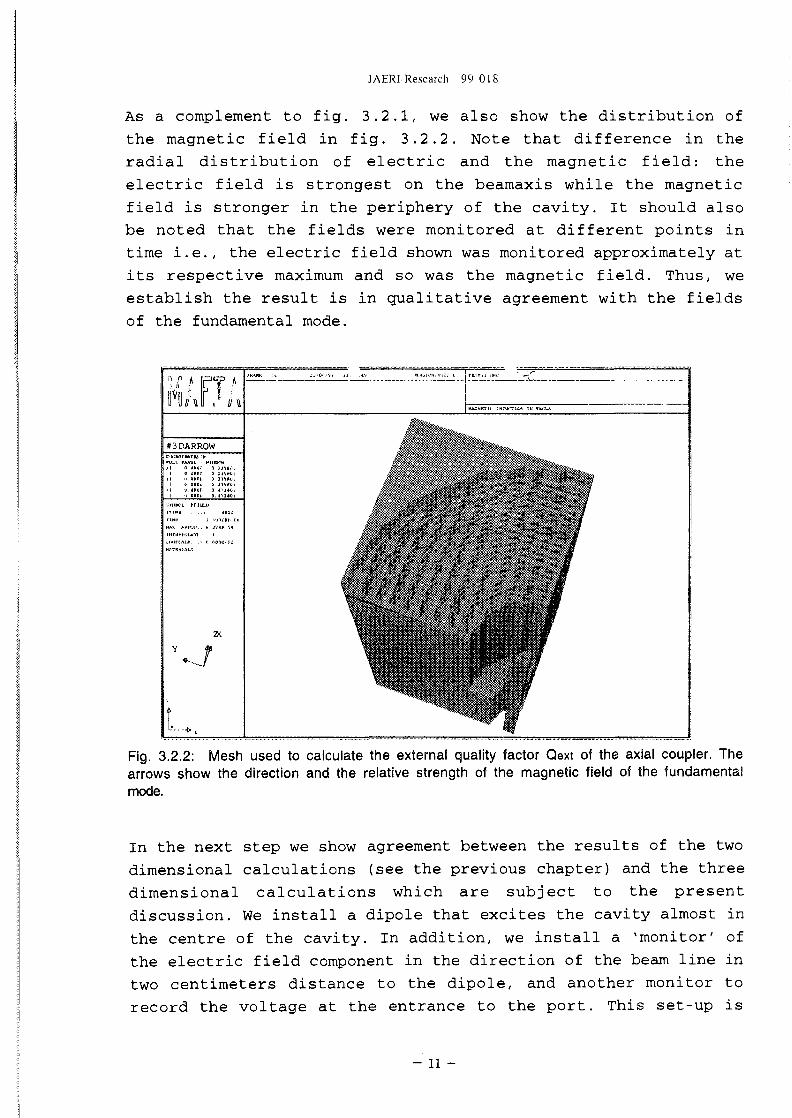
As a complement to fig. 3.2.1, we also show the distribution of

the magnetic field in fig. 3.2.2. Note that difference in the

radial distribution of electric and the magnetic field: the

electric field is strongest on the beamaxis while the magnetic

field is stronger in the periphery of the cavity. It should also

be noted that the fields were monitored at different points in

time i.e., the electric field shown was monitored approximately at

its respective maximum and so was the magnetic field. Thus, we

establish the result is in qualitative agreement with the fields

of the fundamental mode.

'•/ / Fliu i" ti w

#3DARROW

2X

Fig. 3.2.2: Mesh used to calculate the external quality factor Qext of the axial coupler. Thearrows show the direction and the relative strength of the magnetic field of the fundamentalmode.

In the next step we show agreement between the results of the two

dimensional calculations (see the previous chapter) and the three

dimensional calculations which are subject to the present

discussion. We install a dipole that excites the cavity almost in

the centre of the cavity. In addition, we install a 'monitor' of

the electric field component in the direction of the beam line in

two centimeters distance to the dipole, and another monitor to

record the voltage at the entrance to the port. This set-up is

- 11 -

This is a blank page.


almost identical to the one used to document the results of the

calculations in two dimensions. The only difference is that we

cannot install the dipole directly in the cavity centre because -

due to our exploitation of the symmetry of the cavity - the centre

is also a corner point of the numerical mesh.

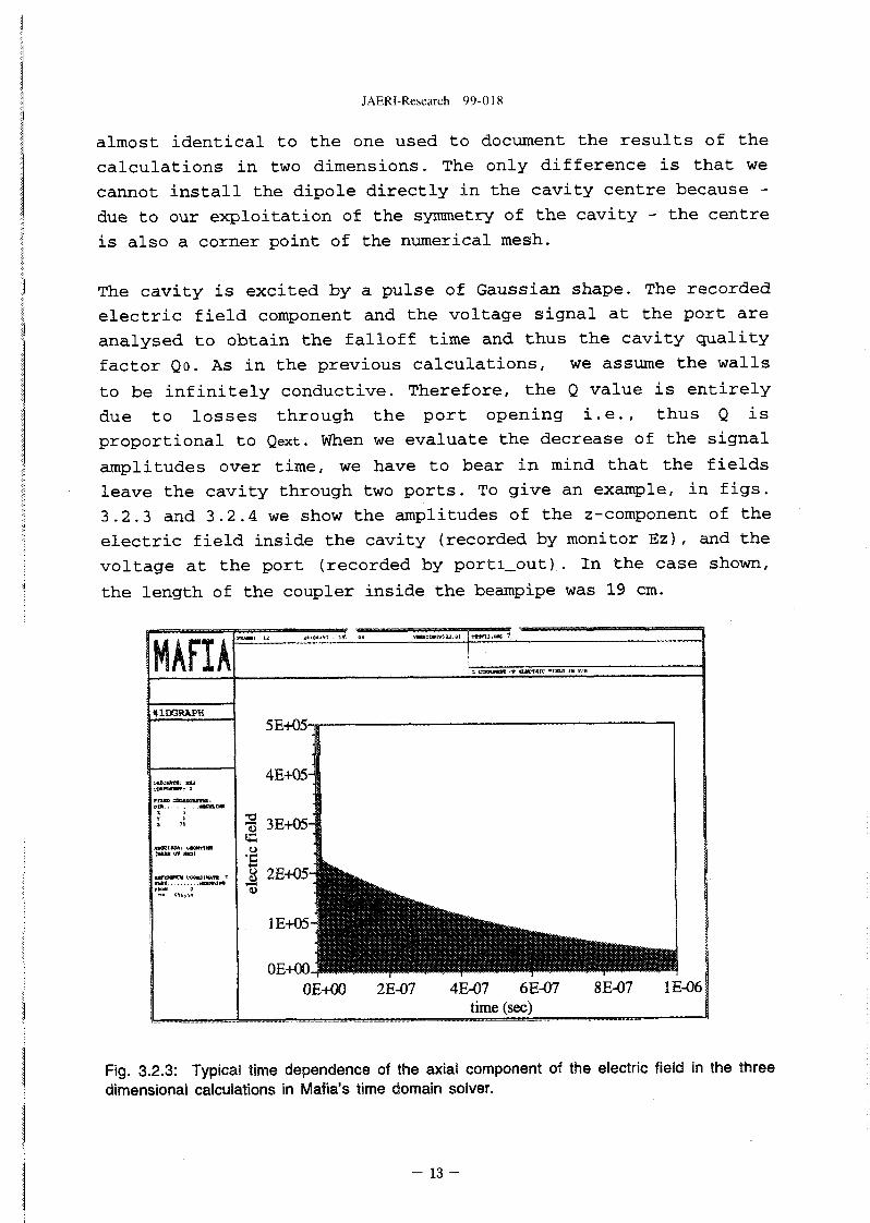
The cavity is excited by a pulse of Gaussian shape. The recorded

electric field component and the voltage signal at the port are

analysed to obtain the falloff time and thus the cavity quality

factor Qo. As in the previous calculations, we assume the walls

to be infinitely conductive. Therefore, the Q value is entirely

due to losses through the port opening i.e., thus Q is

proportional to Qext. When we evaluate the decrease of the signal

amplitudes over time, we have to bear in mind that the fields

leave the cavity through two ports. To give an example, in figs.

3.2.3 and 3.2.4 we show the amplitudes of the z-component of the

electric field inside the cavity (recorded by monitor Ez), and the

voltage at the port (recorded by porti_out) . In the case shown,

the length of the coupler inside the beampipe was 19 cm.

MAHA#1DGRAPH

riZKD COUtDHUVtt ion . . wnR.cn>

% ir t& TS

(•MB 1* K1O1

F i t * V

nuuMi

ield

o

8

5E+O5-J

4E+05-

3E+05-

T105 •In

1E+05-9H

OE+OO-PPfi0E+00

1 ViMalCSlV) 1 ! . SI • m m , EMC 1

z. oTwanw rr OJKtHK Pitto at v/M

^ 1 12E-07 4E-07 6E-07 8E-07

time (sec)1E-06

Fig. 3.2.3: Typical time dependence of the axial component of the electric field in the threedimensional calculations in Mafia's time domain solver.

- 1 3 -


MAHA• 1DGRAPH

DIM HIM 1 m

LBUK or »om_wr3

fOOTKKNCX COOWTKWW; VVAKI ...MUMLIHB

TO 4SSi iO

m w i i j*/o*^T - lev .0) vnci

BMTUt &n»/M 4.*lMI)«tiiIS41-ai

50-j

40-

i3o B k1 2 0 J H H |

OE+OO jWWiW^^WOE+00 2E-07 4E-07 6E-07

time (sec)8E-O7 1E-06

Fig. 3.2.4: Typical time dependence of the port voltage in the three dimensional calculations inMafia's time domain solver.

fall-off length: 23.2 mm106. , t • , . , ,

MWO

105

104

1030.1 0.12 0.14 0.16 0.18 0.2

coupler Jeng th/m

0.22 0.24

Fig. 3.2.5: Qext versus the length of the axial coupler inside the beampipe. The value of Qext isobtained from the falioff time of the z-component of the electric field inside the cavity, (x)mark the values obtained by a MAFIA calculation in two dimensions, (o) those values resultingfrom a calculation in three dimensions.

- 14


The values for Qext versus the length of the coupler inside the

beampipe which result from the calculations in two dimensions and

the calculations in three dimensions are shown in fig. 3.2.5.

They are in excellent agreement.

However, it should be noted that there is a difference between

these Qext values and those resulting from calculations shown in

the previous chapter, figs. 2.2.2. There, the Qext values are

higher as if the coupler were shorter by almost two centimeters.

One explanation could be that we changed the radius of the coupler

in the beampipe. In the calculation of the previous chapter we

modelled the superconducting cavity (niobium cavity) of which the

coupler radius is 7.7 mm. In the calculations presented here, we

model the normal conducting cavity (copper cavity) of which the

coupler radius is almost one centimeter larger: 17.2 mm.

Measurements on a cavity with an axial coupler

4.1 Measurements on an axi-symmetric normal conducting cavity

In order to validate the results of the calculations presented in

the previous Sections we have conducted measurements on a single

cell cavity similar to the one modelled in the calculations. The

cavity design is shown in fig. 4.1.1. The cavity itself is shown

in fig. 4.1.2.

In order to obtain a full understanding of the cavity's electro-

dynamic properties we have conducted three series of measurements:

First of all, in series (A) we measured the reflection coefficient

at the entrance to the axial coupler while the port to the

beampipe of the opposite side was closed, the situation shown in

fig. 4.1.1. By inserting 'outer conductor spacers' that added to

the length of the outer conductor we in effect varied the length

of the axial coupler inside the beampipe which, in fig. 4.1.1, is

shown on the right side.

- 1 5 -


In the second series, (B), we inserted an axial wire probe such as

shown in fig. 4.1.3; this probe, in fig. 4.1.1, would be drawn

protruding through a port on the flanges that close the beam pipe

section on the left side. We measured the scattering parameter

corresponding to the wire probe for varying lengths of the axial

coupler.

In the third series, (C), we varied both parameters, spacer length

and wire length.

53?

Outer conductor spacers

50 ohm n-type adaptor

Fig. 4.1.1: Single cell cavity with axial coupler. One main characteristic is that the 77mmouter conductor of the 50 Ohm feed line can be changed in length by the insertationfrgg++ ofspacers. Thus the protruding length of the center conductor into the beam pipe can be varied.

To evaluate the measurements of series (A) and (B) we determine

the values of cavity Q, denoted by Qo, and the values of Qext of

the coupler, Qext, by an analysis of the impedance curve such as

plotted on the Smith chart in fig. 4.1.4. In order to determine

the frequencies which are required for the extraction of Qo, Qext

and QL, the resonator load has to be moved into 'retuned short'

position. In this position the impedance tends towards zero the

further the frequency is away from the resonance. Hence, in order

to analyze the measured data, the phase of the measured reflection

coefficient has to be offset accordingly.

-16-


cavity beampipe flange 50 Q. line axial coupler

Fig. 4.1.2: Single cell copper cavity with an axia! coupler during the set-up for normalconducting measurements. The flanges between the beampipe and the 50 Ohm feed line can beseen and also the feed line itself. The centre conductor of the feed line is about to be inserted. Itstip will protrude into the beampipe to constitute the axial coupler. The length of the coupler canbe reduced by inserting 'spacers' i.e. additional pieces of outer conductor at the position where,in the picture, the feed Sine is opened.

Fig. 4.1.3: One of the wire probes used in the measurement series (B) and (C).

- 17 -


t.0

-1.0

Fig. 4.1.4: Smith chart with an impedance curve such as obtained in the measurement series.The values of Q0, Qext and QL are found by division of the resonance frequency by thedifferences If5-f6l, If3-f4l, and If1-f2!, respectively.

In figs. 4.1.5, we show typical curves resulting from such

measurements. The graphs in the box on the left side correspond to

a case of overcoupling (Qext < Qo), and those in the box on right

side correspond to a case of undercoupling (Qext > Qo). Note the

difference in the phase curve of the reflection coefficient in the

cases of overcoupling and undercoupling. At resonance, the phase

in the case of overcoupling does not change while in the case of

undercoupling it changes by n. The respective behaviour of the

coupler is that of a line terminated in an open circuit, and that

of a line terminated in a short ciruit.

- 18 -


0.5

la)

(b)11

A1 Aft: JL.

-0.55.862 5.863 5.863 5.864 5.864

flHz

Figs. 4.1.5: In the boxes typical curves are shown of: the normalized amplitude of the reflectioncoefficient (a), the phase of the reflection coefficient, offset and normalized to n (b), thenormalized real and imaginary parts of the impedance curve, respectively (c) and (d), and thenormalized susceptance curve (dashed line, e). The boundaries which mark the frequencyintervals to determine Qo and Qext are marked respectively (o) and (x). In the box on the leftside we see the case of overcoupling, on the right side we have undercoupling.

In measurement series (B) we first excite the cavity and then we

measure Qext of the coupler. The excitation of the cavity is

accomplished by a thin wire probe inserted axially in the beampipe

opposite to the axial coupler which we wish to examine.

First, we determine Qo of the cavity while the axial coupler at

its entrance is terminated in a short circuit (Qo = 22602). Then

we connect the measurement cable to the axial coupler. Thus, when

we use the wire probe to measure the value of Qo', this value

corresponds to the combined effect of the cavity Qo plus that of

Qext of the axial coupler. Both quantities contribute to the losses

that are expressed by Qo' . Hence, we can extract Qext from Qo' :

1/Qext = 1/Qo' - 1/Qo. (1)

During the measurement series (B) we measure Qext for various

lengths of the coupler inside the beampipe. The results of these

measurements are shown in fig. 4.1.6. As a reference, we plot the

results for Qext obtained from the (phase-shifted, but otherwise

uncorrected) reflection coefficient of the axial coupler, i.e.,

measurement series (A) . The falloff length of the coupling

obtained from these measurements is 18.6 mm. Note that the results

of the measurement series (B) agree well with those of series (A).

-19-


external Q of axial coupler

&

105

104

1 1

Mil

iiiiii i i

s : : : : : : : : : :

11 1

J

" fr

::::::::::::#:::I:*!::::

:::

* . .

: : : : : : : : : :

. .„. . . . ,

: : : : : : : :

x- •i

: : : £ : : :

•if

i ; $ i ; i ; ; • • •; • =

;

: : : : : : : : : : : : : : : :

0.04 0.05 0.06 0.07 0.08 0.09 0.1 0.11 0.12spacer length: z/m

Fig. 4.1.6: Results of measurement series (A) and (B). Qext of the axial coupler is plottedversus the length of the coupler spacers. Long spacers cause the coupler to be short inside thebeampipe. The values measured in (A) (reference values) are plotted with (x). They wereobtained by offsetting the phase of the coupler reflection coefficient. The values plotted with(*) were obtained from Qo'(QO, Qext), measured with a wire probe opposite to the axialcoupler.

Finally, we conduct the measurement series (C) to see whether the

length of the wire probe would have any significant effect on the

results for the falloff length and the absolute values of Qext of

the axial coupler.

The length of the wire probe is chosen such that its coupling is

approximately critical. Hence, a reduction of the length of the

axial coupler (by the insertation of longer spacers) requires the

wire probe to be shorter as well. In Fig. 4.1.7 we show which

combinations of wire length and spacers are used in the

measurement series (C) . The rate of change is Alenwire/Alenspacer ~ -

0.9; however, it should be noted that this linear approximation

can only be valid over a small range of wire length (we chose 75

to 100 mm to obtain the value stated above). The reason for this

limitation is the dependence of the measured Qo' not only on the

external quality factor of the axial coupler but also on the Qo of

the cavity as expressed in equation (1).

- 20 -


0.220.21

0.20.190.180.170.160.150.1J

•x *

i

* * • • -x-

04 0.05 0.06 0.07 0.08 0.09 0.1 0.11 0.12spacer length 1/m

Fig. 4.1.7: Combinations of wire length and spacer length used in measurement series (C). Thelength of the wire probe was reduced in step with the increase of length of the spacers on theaxial coupler such that the coupling of the wire probe was approximately critical.

The values for Qext obtained in the measurements of series (C) are

shown in fig. 4.1.8. They are in good agreement with the results

of the reference measurement shown in the same graph. The falloff

length of the coupling is 1 = 15.6 mm. Thus, we have established

the equivalence of the various methods, (A) , (B) and (C) , to

measure the value of Qext of the axial coupler that is best

regarded as a probe.

^ 06 external Q of axial coupler

x&

105 :

104 =

103

rTiT

m

-;:::::::;:

iiiiii

- i

;;;;;;;;;;;;

; ; • • ; • • ; ; ; ; ;

r

jiiim::::!1

;;;;;;;;;;;;

I.....T.....

;;;;;;;;;;;<

f

;;;;;;;;;;;j

&

o

0.04 0.05 0.06 0.07 0.08 0.09 0.1spacer length: zlm

0.11 0.12

Fig. 4.1.8: Results of measurement series (C). Qext of the axiai coupler is plotted versus thelength of the coupler spacers. Long spacers cause the coupler to be short inside the beampipe.The reference values are plotted with (x). The values obtained for a variety of wires with theirlength being different are plotted with (o).

- 21 -

4.2


Comparison of calculations and measurements

In the previous chapters we presented the results of coupling

calculations obtained using the MAFIA time domain solver. In

Section 4.1 we reported the results of measurements conducted to

determine the value of the external quality factor Qext of an axial

coupler in a single cell cavity. In this Section we compare the

results of calculations and measurements.

Fig. 4.2.1 shows the results of both the calculations and the

measurements. The figure shows that the agreements between

calculated and measured results are very good. The coupling

falloff lengths of the external quality factor as the coupler tip

were estimated from the calculations and measurements to be 17.8

mm and 17.3 mm, respectively, which are also in good agreement.

10*

icr

104

10

external Q of axial coupler

I ' ' ' ' r

I I I I I I I I I I I I I I I I I

0.04 0.05 0.06 0.07 0.08 0.09 0.1 0.11 0.12

Spacer length (m)

Fig. 4.2.1: Qext of the axial coupler versus the length of the outer coupler spacers. Themeasurement results are marked (x), the results obtained from calculations with Mafia's two-and three dimensional time domain solvers are marked with (o).

- 2 2 -


5 The superconducting cavity with a sidle coupler

5.1 introduction to the superconducting cavity with a side coupler

In chapter 4 we have established the agreement of measured and

calculated values of Qext in the case of the axial coupler. However

the ultimate goal is to determine, for a design value of Qext, the

shape and position of a side coupler, which will be applied to the

actual accelerator system. For this reason, to show the agreement

between measured and calculated values of Qext in the case of a

side coupler shall be the aim of this section.

beampipe flange cavity side coupler beampipe spacers

Fig. 5.2.1: Single cell copper cavity with a side coupler for normal conducting measurements.Between the cavity and the beampipe a flange can be seen. The side coupler is connected per-pendicularly to the beampipe. Its distance to the cavity can be modified by changing the ioactionof spacers from the endplate, as shown on the right, to the flange between cavity and beampipe.

- 2 3 -

5.2


Measurements to determine the side coupler's external Q

For the purpose of the measurements on a side coupled cavity we

modified the copper cavity, shown in fig. 4.1.2, which we used for

the axial coupler measurements. The modified cavity is shown in

fig. 5.2.1. The coupler, familiar to us from the axial coupler

measurements, is now fixed on the beampipe perpendicular to the

cavity axis. This is shown in the drawing of fig. 5.2.2. For a

view of the coupler from the inside of the cavity see fig. 5.2.3.

The beampipe is cut off the cavity. The connection between the

cavity and the beampipe is made by flanges. Note that the distance

of the side coupler to the cavity can be varied by inserting rings

between the cavity and the beampipe. The spacers which are not in4use' are inserted between the beampipe and its endplate in order

to keep constant the length of the beampipe from the cavity to the

endplate.

Fig. 5.2.2: Single cell copper cavity with a side coupler for normal conducting measurements.We denote the direction of the beamaxis (the on-axis distance) 'z'. The perpendicular directionpointing into the beampipe is called 'y'. Note the reference positions on z and y axis: z =0 at theiris on the coupler side of the cavity where the beampipe flange is welded to the cavity; y = 0 atthe wail of the beampipe on the side of the pipe where the coupler is welded onto the beampipe.

- 24 -


cavity nange siae coupler oearrppe

Fig. 5.2.3: Inside view of the single eel! copper cavity and the beampipe with a side couplerprepared for norma! conducting measurements. The flanges between the cavity and thebeampipe are a bit hard to see. In the text, we frequently refer to the 'on-axis' distance of thecoupler to the cavity. This distance is indicated in the picture by the double flesh.

Concerning the opposite side of the cavity, there the beampipe is

not modified with respect to the set-up used during the axial

coupler measurements. As in those measurements, a wire probe is

mounted on the beamaxis. The Hewlett Packard network analyzer is

connected to a wire probe which is excited by the analyzer's

signal (port 1). The transmitted signal is picked up from the side

coupler and recorded by the analyzer (port 2). The evaluation of

the measured data is done as discussed in chapter 4 in order to

extract the values of cavity Qo, Qext of the wire probe, and

ultimately the external quality factor of the side coupler.

Note that our set-up of the side coupled cavity permits us to vary

both parameters, the length of the coupler i.e., the distance of

the coupler tip to the wall of the beampipe, and the on-axis

distance of the coupler to the cavity, cf. figs. 5.2.2. and 5.2.3.

The measurement results of Qext of the side coupler are presented

below. In fig. 5.2.4 we show the values obtained (for several

settings of the coupler length) while the coupler's on-axis

distance is varied. In fig. 5.2.5 we show the values obtained (for

several settings of the on-axis distance of the coupler) while the

coupler length was varied i.e., the distance of the coupler tip to

the wall of the beampipe.

- 25 -


108

107

&

105 :

104

X

+

rm

*

X

• : : : : : : : o : : : : ;

* :

X

+

: : : : Q : : : : : : :

. «

.X

"4

»••: : -

X"

::::::::::$::

o

::::«:::::::

: : : :^: : : : : : :

Liii

O

uli

80 85 90 95 100 105

coupler distance to cavity (zlmm)

110 115

Fig. 5.2.4: Measured values of external quality factor Qext of the side coupler to the normalconducting cavity versus the on-axis distance of the side coupler to the cavity. The radialdistance of the side coupler's tip to the beampipe wall is (y/mm): 40 (o), 20 (+), 0 (x), and-20 (•).

-20 -10 0 10 20 30 40

side coupler tip distance to beampipe vail (ylmm)

Fig. 5.2.5: Measured values of external quality factor Qext of the side coupler to the normalconducting cavity versus the radial distance of the side coupler's tip to the beampipe wall. Theon-axis distance of the coupler to the cavity is (z/mrn): 80 (*), 88 (x), 96 (+), 104 (o),and 112 (•).

- 26


Note that in fig. 5.2.4 we observe an exponential rise of the

coupler's Qext value when the coupler's on-axis distance to the

cavity is increased. The rate of increase does not depend on the

actual length of the coupler tip. Moreover the falloff length of

the coupling (X = 15.4 mm) appears to be in reasonable agreement

with the results obtained in the course of measurements on the

axial coupler (X' = 17.3 mm), cf. chapter 4.

We turn our attention to fig. 5.2.5 which shows the dependence of

the coupling on the length of the coupler i.e. the distance of the

coupler tip to the wall of the beampipe. We distinguish between:

a) the cases where the coupler is protruding sidewise into the

beampipe, and b) those where the coupler is recessed inside the

feed line; the latter are those cases where the distance between

the coupler tip and the beampipe wall is negative.

Concerning the cases a) we do not observe an exact exponential

drop of Qext when the coupler tip is extended towards the beamaxis.

However, in the cases b), where the tip is well recessed in the

feedline, the values of Q can be interpreted to rise exponentially

as the distance between the coupler tip and the beampipe wall is

increased. Under the assumption of an exponential dependence on

the coupler length in b) the falloff length is X" = 8.4 mm.

5.3 Calculation of the side coupler's external quality factor

For the purpose of the calculation of the value of the external

quality factor Qext of the cavity we use a three dimensional grid,

shown in fig. 5.3.1, which is similar to the one used in the case

of the axial coupler, cf. fig. 3.2.1. Note that the side coupler

can easily be accommodated without an enlargement of the grid

block. Rather, the block has become smaller as the feedline on the

cavity axis is omitted. Note that the ratio of coupler fraction to

cavity volume is half a coupler in one eigths of a cavity (axial

coupler: a quarter coupler in one eighth cavity). Hence, the

falloff time of the field inside the cavity is calculated four

times too short and we have to multiply the corresponding Q value

by a factor of four in order to obtain Qext of one side coupler.

- 2 7 -


Fig. 5.3.1: Grid used to calculate the external quality factor Qext of the cavity. To fully exploitthe rotational symmetry (apart from the side coupler), the grid comprises one eighth of thefull cavity and one half coupler. The arrows indicate the direction of the electric field of thefundamental mode.

We optimise the calculation method which was applied in the case

of the axial coupler, cf. chapter 4. Once we establish the

relation between the falloff time of the field inside the cavity

and the peak voltage at the port to the cavity the optimisation is

achieved by obtaining Qext in all further calculations from the

maximum voltage amplitude U at the port of the feedline. See

Section 2.3 for a detailed account of the full Q evaluation

method.

We have conducted an extensive series of calculations while

scanning both parameters, the on-axis distance of the side coupler

to the cavity and the distance of the coupler's tip to the wall of

the beampipe. The results are shown in fig. 5.3.2. Note that we

can observe the coupling to decrease exponentially with increasing

on-axis distance of the coupler to the cavity. The falloff length,

X - 16.4 mm, is independent of the coupler setting.

- 29 -


109

xo

104

: : : ! : ! : : : : : : j? : : : : : : : : : : : : \% i i i : : : : : : : : : : j : : : i : : : : : £ : : 1 1 | : : ! : : : : : : : : i : f : : ! : : T T T T T T T T T : ! : : : : : : : : : : :

• : • • • • • : • ; • ; • : : ; ; : ; : ; ; ; ; ; ; ; : • • • • • : • • ; • • • •

J • • • • • • • : • • • : • < • :::>:::::•;•••:•:>:;••••:;•::•

:::::::::':::: r::::::::::::: r::::::::::;::

80 90 100 110 120 130 150

z/mm

Fig. 5.3.2: Values of Qext calculated for the side coupler mounted on the beampipe versus theon-axis distance of the coupler to the cavity. The results correspond to various settings of thecoupler. The distance of the coupler tip to the wall of the beampipe is (y/mm): 40 (*), 20(x), 0 (+), and -20 (o).

Xa>O-

105

104-20 -10 10 20 30

z/mm50

Fig. 5.3.3: Values of Qext calculated for the side coupler mounted on the beampipe versus thedistance of the tip of the side coupler to the wall of the beampipe. The results for various on-axis distances of the side coupler to the cavity are shown (z/mm): 65 (•), 50 (*), 35 (x), 20(+), and 5 (o).

- 31 -


In fig. 5.3.3 we show the same calculation results, however, the

values of Qext are plotted versus the distance of the side coupler

tip to the wall of the beampipe. We distinguish between: a) the

cases where the coupler is protruding sidewise into the beampipe,

and b) those where the coupler is recessed inside the feed line;

the latter are those cases where the distance between the coupler

tip and the beampipe wall is negative.

Concerning the cases a) we observe a decreasing rate of drop of

Qext when the coupler tip is extended towards the beamaxis.

However, in the cases b) , where the tip is well recessed in the

feedline, the values of Q can be interpreted to rise exponentially

as the distance between the coupler tip and the beampipe wall is

increased. Under the assumption of an exponential dependence on

the tip distance to the wall b) the falloff length is X' = 9.3 mm.

5.4 Comparison of calculated and measured values of Qext

We now shall compare the results of measurement and calculation,

discussed in Sections 5.2 and 5.3, respectively, concerning the

value of external quality factor of the side coupler to the normal

conducting cavity. In fig. 5.4.1 we show the values of the coupler

Qext for various settings of the coupler length. Note that the

agreement within the uncertainty of the measurement is very good

over the full range of the coupler distance.

Considering the results, we should also bear in mind that there is

still room for more precise measurements by narrowing the

frequency band in which the network analyzer excites the cavity.

Concerning the calculations we can easily afford to refine the

grid at the cost of higher calculation times because of the

introduction of the peak port voltage reading method, discussed in

Section 2.3.

- 3 2 -


109

109

107

106,=

105

104

• • • • • ; ; ; ; ; =

= • • • : • • • ? { • <

imn

£ x<i:::::::*:'I

; ; • : ; ; ; ; ; • ; ; !

I : : : : : : : : : : :

:::::x

X (

P l i l l l l l l l l l

x . . J9

j i i l i i i x : : : '

' • ; : : : : : : : i : > : : : : : : : : : : : : 1

: : : : : : ; : : : : r : : : : : : : : : : : :

• x t» X H>n::::::!:::t::::!:::::::::::::::::: :::::::::::::

• ic ia *

> X 7l l l i l i l i l l i H i l l i i l l l l i l

':s..lits,:::..Lx ::J

m

::::::::::::

• • • • • • • : : : : :

x-\Mi!;;!;!;;!

* * •

! : : : : : : ! : : : :

; : : : : : : : : « :

f..

; • • • • • • • • ; • •

: : : : ! : i : : : : :

; ; ; ; ; ; • ; • • • •

: : : : : : : : : : : :

. : : : : : : : : • : :

> y

! : : : • : : : : : : :

:::: M ::::::

;:::x:::::5::::::::::::

• : : : : : : : : : : 1J ; ; • -

• • • • ; • : • • • ; =• : : : ! : : : : : : :

i l l l l l l l i i l i

>

: :::: s'.:::::::::::

80 85 90 95 100 105 110 115 120

on-eocis distance of side coupler to cavity z/mm

Fig. 5.4.1: Measured (x) and calculated (o) values of Qext of the side coupler obtained forvarious settings of the coupler tip distance to the wall of the beampipe (y/mm): 40 (a), 20(b), 0 (c), and -20 (d); the negative distance in (d) corresponds to the case where the tip isrecessed inside the feedline of the side coupler.

However, more refined methods of either measurement or calculation

are hardly required for we have well established the falloff

lengths corresponding to the parameters which enter the design

considerations: the distance of the side coupler to the cavity and

the protrusion of the coupler tip into the beampipe. Furthermore,

the fact that, in the calculation, we fully exploit symmetries to

keep the size of the grid small does not appear to have any

noticeable effect onto the validity of the resulting Qext values.

Perhaps an exception to this rule are those cases where the

coupler tip protrudes close to the beamaxis. The coupler in such

cases 'sees' its mirror image which in the true geometry, of

course, is not implemented. We reckon that the tip's protrusion

has to exceed 30 mm into the beampipe for the mirror effect to

become noticeable. However, such far protrusion has little

practical relevance.

- 3 3 -


Conclusions

Using the time domain solvers of Mafia, we have calculated in two

and three dimensions the quality factor Qo of a single cell copper

cavity of the superconducting high beta section of the accelerator

which is proposed for the Neutron Science Project of the Japan

Atomic Energy Research Institute (JAERI) by the Proton Accelerator

Laboratory group.

We have calculated, using Mafia's time domain solvers, the Qext

values of an axial coupler in the beampipe to the accelerator

cavity. Moreover, we have calculated the Qext values of a side

coupler mounted onto the beampipe to the accelerator cavity.

Measurements were conducted in all cases and the calculation

results were found to agree well with the measured values. Hence,

we have established the Mafia calculation, in particular of the

side coupler's external quality factor, as a valid tool that can

be reliably applied to establish certainty about the electrical

qualities of a side coupler under design for the accelerator.

- 3 4 -


Appendix

A.1 A two dimensional model of the superconducting cavity

The cavity constitutes a two-port. We would like to calculate the

scattering parameters using Mafia's eigenmode solver. In order to

do so we choose the time dependence of the input signal in

accordance with the Mafia instruction manual i.e.,

f (t) = sin(an) sin(an/2) • 0.75 • 3 for 0 < an < 2%, or

f(t) = 0 otherwise,

where co = 4JC fres and x = t in the case. We begin the pulse at the

start of the simulation. The pulse length is one oscillation

which, however, is not just sinusodial. The exciting signal i.e.,

the forward voltage at port one, U^or, is shown in fig. A.1.2. Its

duration is that of a half cycle of the resonance frequency, which

is less than one nanosecond.

Parts of the coaxial feedlines on either side of the cavity are

included in the simulation area. The signal Uref returning at the

entrance to the coaxial feedline and the signal transmitted

through the cavity and obtained up at the pick-up exit Utrans is

shown in figs. A.1.3 and 4, respectively.

Concerning the output signal Uref we note, first of all, that a

time delay At occurs between the input signal and the reflected

signal. Assuming that waves in the coaxial waveguide propagate

without dispersion at the vacuum speed of light we can obtain the

length 1 of the coaxial guide: 1 = c At/2 » 0.195 m which is in

good agreement with the programmed value (l'= 0.18 m plus the tip

length of 0.02 m inside the beampipe). Secondly, we note that the

amplitude of the reflected signal at port one is falling off

during the observed time interval. Nevertheless, we are able to

observe the signal for a much longer time span than the duration

of the input oscillation. In order to estimate the frequency of

the "reflected" signal we simply count the number of peaks and

divide by the observed timeinterval: festimate = 53/(3e-8 - 0.25e-8)

Hz ~ 1.9 GHz which is well above the fundamental resonance of the

cavity at approximately 580 MHz.

- 35-


MAFIA#1DGRAPH

0.5-

OE+00-

-0.5-

OE+00 5E-10 1E-09 1.5E-09 2E-09 2.5E-09 3E-09time (sec)

Fig. A.1.2: The pulse signal we use in Mafia's time domain solver to excite the cavity.

MAHA#1DGRAPH

TITO. COCASl

V I

OE+00

-0 .5-

OE+00 5E-9 1E-08 1.5E-08 2E-08 2.5E-08 3E-O8

time (sec)

Fig. A.1.3: The signal reflected at the exciting port to the cavity.

- 3 6 -


MAFIA• K S AMVl ITOK Hi

#1DGRAPH

PtUD COCCI'<«*TKS:5E-02-

0E+00

-5E-02-

-0.10E+00 5E-9 1E-08 1.5E-08 2E-08 2.5E-O8 3E-08

time (sec)

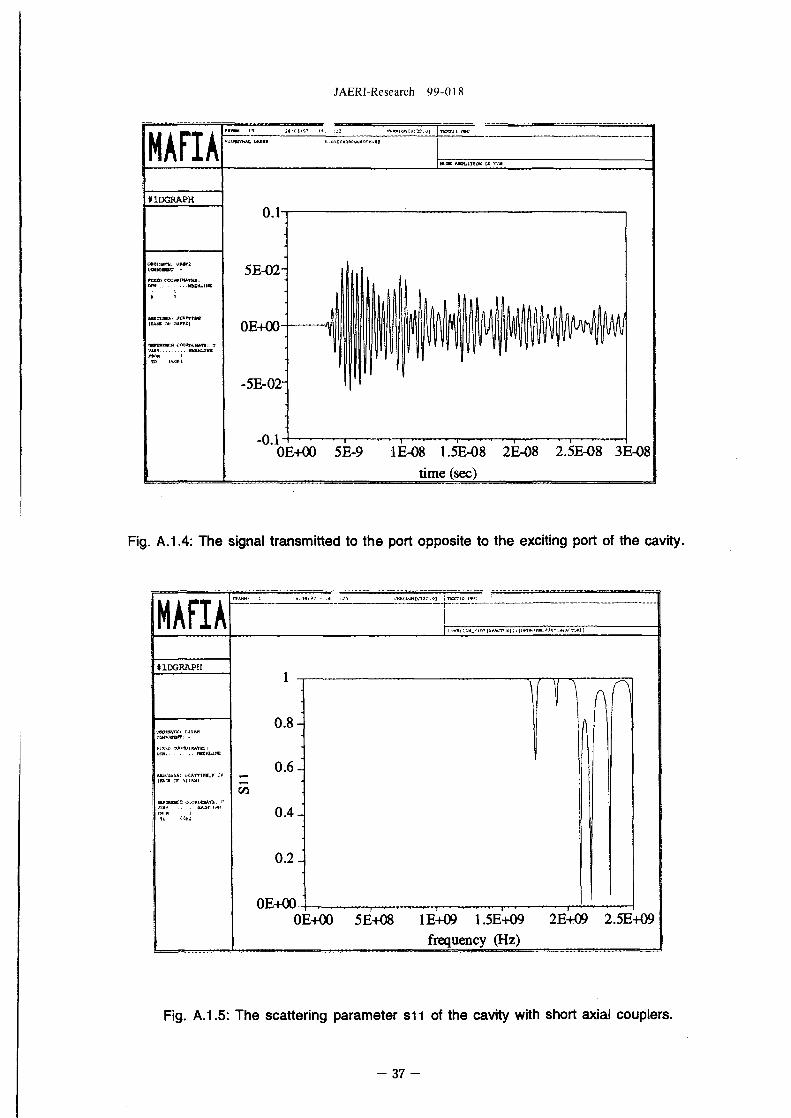
Fig. A.1.4: The signal transmitted to the port opposite to the exciting port of the cavity.

MAHA41DGRAPH

UTOIHMVi ijllMl

VWiO ';(k.ia.iKATiei;

AteCtuif,: (.(ATtiKI.I' .!"•'i n , : i r r v i iu i i

VMIV. . . . . . HlWIl.lNK

11 -

0.8-

0.6-

0.4-

0.2 i

OE+00OE+00 5E+08

1

1E+09 1.5E+09

frequency (Hz)

2E+0S

A

) 2.5E+O9

Fig. A.1.5: The scattering parameter S11 of the cavity with short axial couplers.

- 37 -


In fig. A.1.5 the amplitude of the scattering parameter sn is

shown. Note the absence of resonant absorption at the frequency of

the fundamental cavity mode. Apparently, "knocking onto" the

cavity with a short pulse does not lead to an excitation of the

fundamental mode. We assume the value of Qext of the fundamental

mode, Qfundext, is much higher than the corresponding value of the

i-th higher order mode (HOM, hence QiH0Mext) . Consequently, it takes

a longer time to fill the cavity with field energy corresponding

to the fundamental mode than it takes in the case of the HOM.

Thus, we expect that the overwhelming part of the energy provided

by a short pulse should be stored in HOMs with low Qext values. In

particular, we bear in mind that the fundamental mode does not

propagate in the beampipe. The coupling to the fundamental mode

should therefore be much reduced with respect to the coupling to

such HOMs which propagate in the beampipe.

In order to check our assumptions we extend the tip of the inner

conductor of the coaxial feed line well into the beampipe as shown

in fig. A.1.6. We repeat the excitation with the same signal as in

the case discussed previously, see fig. A.1.2.

MAFIApSs.ouNjv.Ji2--: I ' ' r

TIMS ilftBMOfrr •3I.KTHC

HARROW

(m)

0.236

0.118

0 0.472 0.945(m)

Fig. A.1.6: The cavity with long axial couplers and the electric field of the fundamental mode.

- 38 -


MAHA#1DGRAPH

55£ 0.6-

0.4 -

0.2 -

0E+000E+00 5E+O8 1E+09 1.5E+09

frequency (Hz)

2E+O9

Fig. A.1.7: The scattering parameter s11 of the cavity with long axial couplers.

The amplitude of sn is shown in fig. A. 1.7. We can clearly see a

peak in the absorption spectrum at 580 MHz. As a result we note

that the inwards prolongation of the centre conductor of the

coaxial cable through all the beam pipe close to the cavity itself

leads to an excitation of a mode at the fundamental frequency.

A.2 Excitation of the superconducting cavity from the inside

In Section A.I we discussed the excitation of the cavity by a

pulse fed via one of the coaxial feed lines. Now we examine the

response due to an exciting electric dipole placed inside the

cavity. We observe the voltage signals which emerge from the

cavity. We stick to the practice to label the signals "reflected"

while bearing in mind that the signal source is inside the cavity:

hence the "forward" voltage signal on either port is zero because

no voltage wave is incident to the cavity.

In this Section we examine the cavity with the probe tips in their

standard recessed position while in the following Sections we

- 3 9 -


shall discuss the cavity with the tips protruding far into the

beam pipe. We conduct two kinds of calculations. The difference

between the calculations is the shape of the signal exciting the

cavity. We observe the component Ez of the electric field in the

direction of the cavity axis. To do so we install "monitors" on

the beamaxis. In Mafia, monitors can record the values of field

components as the calculations proceed in time.

MAFIAPKMtti 4 J1/3V»1 - 15'. I )

0 .4OM4000MUOOBHKI

#1DGRAPH100

13

0E+00-

-1000E+00 2E-09 4E-09 6E-09

time (sec)

8E-09 1E-08

Fig. A.2.1: Component of the electric field in the axial direction recorded with monitor Ez whenthe cavity is excited with a pulse signal by the dipole in the centre of the cavity.

Signal shape A) is a single oscillation (T < 1 ns) such as used in

the previous Section, cf. fig. A.1.2. The single oscillation ex-

cites the cavity over a broad frequency spectrum. In fig. A.2.1 we

see how the perturbation of the pulse (see signal at t < 0.8 ns)

causes the field Ez to oscillate. We perform the Fourier

transformation of the signals to obtain the frequency spectrum of

the oscillating field. The spectrum of the field in the frequency

range from 0 to 2 GHz is shown in fig. A.2.2. Note that spikes at

580 MHz and at 1260 MHz indicate the presence of resonances.

- 4 0 -


MAFIA#1DGRAPH

OftDIIMTS: BX3AM_TU

TTJV3 CTOROINUKS;DIM KKSHMM

[SWZt OF n U N _ r U ] ~"

VMTt KHKLMnm u

TO * H J 1

1

ampl

1E-05 -j

8E-06-

•

6E-06-

4E-06 -

2E-06-

OE+00 5E+O8

«™'«r

L1E+09 1.5E+09

frequency (Hz)2E+09

Fig. A.2.2: Fourier spectrum of the electric field component recorded with monitor Ez.

MAHA#1DGRAPH

M B . . . HKbULlNK

1

1

0.5-

-0.5-

0E+00 5E-09

^ A/- vy

1E-08

MuU MtrUtVOC IN

AM

1.5E-08time (sec)

ill-

2E-O8 2.5E-O8 3E-08

Fig. A.2.3: The Gaussian signal we use in Mafia's time domain solver to excite the cavity.

- 4 1 -


MAFIA AIIWAMU. OMMR

Ci» w,Tn-f "* FT1LI) I

tlDGRAPH

2000

1000-

0E+00

-1000-

-2000OE+00 2E-08 4E-08 6E-08 8E-O8 1E-07

time (sec)

Fig. A.2.4: Axial component of the electric field recorded with monitor Ez. A dipole excites thecavity with a Gaussian enveloped sine oscillation.

MAMA#1DGRAPH

I 9-«Do«+li*, a JWiflO]

( 9 ooim.oo, Q.iOM-ai]Mscidiut! iMtunat / . ] (

! 0.0001*40, a.3DM*10] tade

ampl

i

Ih-u4 -

8E-05-

6E-05-

4E-05 -

2E-05-

OE+00

VKBICW1V)32 0]

A/A5E+O8 1E+09

frequency (Hz)1.5E+09 2E+09

Fig. A.2.5: Fourier spectrum of the electric field component recorded with monitor Ez. A dipoleexcites the cavity with a Gaussian enveloped sine signal.

- 42 -


MAFIA umi tva.

#ARROW

•I 3.00DO. 9.3MW)

SI 0.179H, 0.7MMI

ITIHtmm.... ,;

(m)

0.236

0.118

00.180 0.472 0.765

(m)

Fig. A.2.6: Electrical field in the cavity after the excitation by an electric dipole.

Signal shape B) is that of a Gaussian shaped wave package (tpeak <

10 ns) where the frequency is the resonance frequency of the fun-

damental cavity mode. Such a wave package is shown in fig. A.2.3.

The monitored signal is shown in fig. A.2.4. After the Gaussian

dipole signal (i.e., t > 15 ns) we can still observe an oscil-

lating field of the same amplitude. Fourier transforms of the

signal (at two positions inside the cavity) are shown in fig.

A.2.5. The cavity field oscillation after the end of the dipole

excitation can be seen as little "spikes" at 580 MHz. Note that

the Gaussian package does not significantly excite the cavity at

any frequencies other than 580 MHz.

In order to determine the mode we record the full electric field

inside the cavity (and the adjacent beampipe) at 80 ns. At this

time, the electric field can be seen to be at maximum, cf. fig.

A. 2.4. The full field in the cavity is shown in fig. A.2.6. It

looks similar to that in the space between the parallel plates of

a capacitor. Thus, we know to have excited the cavity at the

fundamental TMoio mode. The field is strongest on the beamaxis and

weakest in the periphery of the cavity. In particular, it should

- 43 -


be noted that the strength of the field appears to drop off to

negligible strength in the extremities of the beampipe. We see

that the probe couplers do not really get "in touch" with the

field. As stated in Section A.I, the fields inside the beampipe

are evanescent. This is why coupling an external signal to the

TMoio mode of the cavity is so difficult.

A.3 Excitation of the cavity at non-fundamental frequencies

In Section A. 2 we discussed the excitation of the cavity by

different types of signals emitted from a dipole placed in the

center of the cavity. In this Section we shall complement our

observations by calculating the cavity time response when the

dipole oscillates at frequencies other than the resonance of the

fundamental TMoio mode.

Earlier, we noticed the existence of another resonance than that

of the TMoio mode at a frequency of approximately 1260 MHz, cf.

fig. A. 2.2. Now, we shall excite the cavity at this higher

frequency in the same way as in Section A.2, case B), where the

envelope of the signal was chosen Gaussian. Likewise, we observe

the z-component of the electric field inside on the cavity axis

with Mafia's field monitor.

The monitored field is shown in fig. A.3.1. The time development

of the field proceeds in the way which is already familiar to us

from the calculations at the fundamental mode: At first the

Gaussian shaped dipole signal dominates the observed fields.

However, after the vanishing of the pulse the cavity can be seen

to oscillate at the resonance frequency of the mode.

As a complement we calculate the Fourier spectrum of the voltage

signal emitted from the coaxial ports of the cavity, see fig.

A. 3.2. The resonance is clearly visible in the spectrum. In

addition, we monitor the complete electric field in the cavity at

t = 80 ns. This field is shown in fig. A.3.3. The fact that the

field lines lie parallel to the cavity axis supports the assump-

tion, stated in Section A.2, that the resonance at 1260 MHz

corresponds to the TM020 mode.

- 44 -


MAFIAcaoaam or njEntc rino IN V

K1DGRAPH

USCJ 8S*: OaCHTTMI|BL» at nil

2000

1000-

"OE-KX)

-1000-

-2000OE+00 2E-08 4E-08 6E-08 8E-O8 1E-07

time (sec~>

Fig. A.3.1: Electrical field in the cavity recorded by Ez. An electric dipole excites the cavitywith a Gaussian shaped sine signal at 1260 MHz.

MAFIAttlDGRAPH

2E-10

DUt M

OE+00OE+00 5E+08 1E+09 1.5E+O9 2E+09

frequency (Hz)

Fig. A.3.2: Fourier spectrum of the port voltage when the cavity is excited with a Gaussianenveloped sine signal at the frequency of 1260 MHz.

- 4 5 -


Fig. A.3.3: Electrical field in the cavity after the excitation by an electric dipole at 1260 MHz.

MAFIAs OOWUMMT =r s u i m i c

#1DGRAPH200a

TO 135»>

-2000OE+00 2E-08 4E-08 6E-O8 8E-O8 1E-07

time (sec)

Fig. A.3.4: Electrical field in the cavity recorded by Ez. A dipole excites the cavity with aGaussian shaped sine signal at 950 MHz.

- 46 -


So far, we have shown the results stemming from an excitation of

the cavity at one of its resonances. What happens if the dipole

oscillates at a frequency well apart from a resonance? In order to

answer this question we conducted a calculation where the dipole

oscillates at approximately 950 MHz. The resulting field at the

monitor Ez in the time domain is shown in fig. A.3.4. We can see

the Gaussian envelope of the dipole signal. However, no

significant excitation of the cavity can be observed. Compare this

result to figs. A.2.4 and A.3.1 where the cavity is shown when

excited at its TMoio and TM020 resonances, respectively.

A.4 Protrusion of the coupler into the beampipe of the sc cavity

In Section A. 3 we discussed the excitation of the cavity at

frequencies higher than that of the fundamental mode. At these

frequencies we could observe a tiny voltage signal at the ports to

the cavity resulting from leakage through the coaxial opening, cf.

fig. A.3.2. In this Section we examine the effect of a protrusion

of the centre conductors of the coaxial lines into the beampipe

while the cavity is excited at the resonance frequency. Note that

we have already briefly discussed such a protrusion earlier, when

we calculated the broadband frequency response of the cavity, cf.

Section A.I.

The case similar to the experiment, where the centre conductor of

the coaxial line protrudes only two centimeters into the beampipe,

cf. fig. A.2.6, serves as reference case, labeled (R) . In this

Section, we calculate the case (H) where the centre conductor of

the coaxial feed protrudes by 12 cm i.e., half of the length of

the beampipe, and the case (F), where the conductor protrudes by

22 cm i.e., almost the full beampipe length. In figs. A.4.1 and

A.4.2 the outgoing voltage signal is shown for cases (H) and (F);

mind that, in the reference case (R) , we could not observe any

output signal. Note also that the different scale in figs. A.4.1

and A.4.2: the scale of the graph corresponding to case (F) is ten

times larger than that of case (H).

- 47 -


In case (H) the port signal rises as long as the dipole pulses

inside the cavity (t < 15 ns) . Then its amplitude appears to

decrease slightly (approximately by 1 % in 80 ns). However, the

signal in case (F) where the conductor protrudes the beampipe

almost at full length, first of all, is stronger by almost one

order of magnitude and, secondly, after the time (t < 20 ns) where

the signal's amplitude rises, it appears to decrease markedly (by

almost 20 % in 80 ns). Moreover, we can see that the rate of the

signal's decrease, itself, drops with time, exponentially.

Hence, we conclude that coupling to the fields inside the cavity

is, indeed, improved by the increased protrusion of the centre

conductor into the beampipe. The port voltage signal is in

agreement with the assumption that the field inside the cavity

should drop exponentially as it leaks outside. Concerning the

quality factor Qext of the cavity ports, in order to establish

quantitative results, calculations are needed that cover a longer

time interval than the one observed here (100 ns).

MAFIA#1DGRAPH

3E-O3-

2E-O3-

-2E-03-

-3E-03

i in

0E+00 2E-08 4E-08 6E-08 8E-08 1E-07

time (sec)

Fig. A.4.1: Case (H) where the centre conductor protrudes half of the beampipe. Port voltagewhile the cavity is excitated by an electric dipole at 580 MHz.

- 4 8 -

JAERI- Research 99-018

MAFIAwoe* Mcniiun ut '

ttlDGRAPH

3E-02

VAKI

TO 131

-3E-024OE+00 2E-08 4E-08 6E-08

time (sec)

8E-O8 1E-07

Fig. A.4.2: Case (F) where the centre conductor fully protrudes the beampipe. Port voltagewhile the cavity is excitated by an electric dipole at 580 MHz.

- 4 9 -


A.5 Table of the Side Coupler's External Quality Factor

Values of Qext of the side coupler to the accelerator cavity

z/mm

80

84

88

92

%

100

104

108

112

80

85

90

95

100

115

130

145

y/mra -20

experiment

9423874

14277533

13114172

22846861

37932836

Mafia calculation

8634645

11625541

15710207

21200964

52056362

128629363

325352260

-15

5181329

7426610

4030678

4643520

6905889

9298612

12561461

-10

2342947

2838601

4286075

4126801

6811152

10991863

2313726

2894161

3961483

5345834

7183486

17621724

43514869

110494230

-5

1171621

1620660

2354703

2345987

3821964

6118884

1726472

2281404

3085988

4137920

10141396

25113683

63383727

0

781324

1214167

1354384

1319458

2256803

3524936

5820490

773598

959405

1320823

1776668

2391868

5942139

14529081

36846023

10

260583

331127

506547

489724

798544

1287313

2129656

339191

417917

581163

788546

1073299

3154184

6708118

17305645

20

117262

138908

210143

216739

351295

552975

892061

141264

176217

244272

330206

444167

1115802

2804886

7183486

30

57207

69085

107633

58186

72555

97532

132496

179465

40

30461

36284

54367

57890

89419

143569

230750

36152

45221

61068

82551

112195

276236

679920

1740595

50

18042

20307

34086

23467

31891

43264

58360

79001

- 50 -


A.6 Literature

[1] N. Ouchi et al., "Proton Linac Activities in JAERI", Proc. of

the 8th workshop on RF Superconductivity, Abano Terme, Italy 6-10

Ocotber 1997

[2] N. Ouchi et al. R&D Activities for Superconducting Proton

Linac at JAERI, Proc. of the first Asian Particle Accelerator

Conference, Tsukuba, Japan, 23-27 March 1998

[3] N. Ouchi et al. , "Design and development work for a

superconducting proton linac at JAERI", Proc. of the 8th workshop

on RF Superconductivity, Abano Terme, Italy 6-10 October 1997

[4] MAFIA The ECAD System Operation Manual, The Mafia

Collaboration, 9. December 1996 (http://www.cst.de)

- 51 -

ate

M'fi-ll}

mthis%it

¥•

1

M

nim

SU

fitIMI

tftIIS

iytisftft

Ty

A

7

X

—

a

y

il

y

ft

f 7 A

^ T

r 7

r >

iijj'nfw:

,id >>

in

kgs

A

Kmolcd

rad

sr

S i t R5

IM

H:.x-i:

*

«

IS-f•fe•ftm

anm.u

M

)j

)1 ,

+ , SiW fit ,

* , '11L, i

Sv. fi

y 9' ? 9II •> 0 X

W« Strt "3

IS

S'l *•«1I e

hif/C

y x

IS.y x!u IS

<MIS

S

—

'S

7?-t:7

j ; '

•7

r- X

)U

il

. 1 .

X

r

-x

-

-

/I.

-

-

X

-->

?

u

ft;

h

-

u

7

>

-

1J

/I,

> •

;U

1-y

hKA

X

•5-

>

X

,1

h

HzNPaJ

WCVFQ

SVVbTHC

Imlx

B(|

c-ySv

i; j : 6 ams 'nvkg/s-N/nrN-ni.l/sA-sW/AC/VV/AA/VV-sWl)/nrWb/A

cd-srltn/iir

S - ]

J/kg•1/kR

IS'J

Ki

, U-J, II

, 5)-, #••/ I - ; U

y

{- %• il \~

f-fthtHMv:

min,

1, L1

eVLl

h

'j

, d

1 cV-1.60218xl() '''.I

S i t Jt-U

f, ft-tyfT, V D -/« —/< —A"

u > i- y7

A

>

;l/

-

>

FA

lili i>

Ab

bar

(ialCiR

radrein

1 A = 0.1nm = l() '"m

1 b-100fm-=10 -"m"

1 bar-U.lMPa-10'Pa

1 Cjal=lcm/sL'-10 "in/s2

1 Ci=3.7xl()"'Bq

I R-2.58xlO 'C/kg

1 rad = lcGy-10 -Gy

1 rcm = k-Sv = l() "Sv

fffK

K)1"10lr'

1O1-10"10"10'10-10'

10 '10 -10 :l

10 "10 ''10 '-1 0 '•"

10 K

X. i

fif

\-

T

•T

'US' -It

?7

/ /

A*n

' h

- t >• -f-

-7 i•j-

f7 J

T

'7 a

/

A )•

h

KPTGMkh

da

dcmVn

P

ra

(no1. &\ - 5 li

ISttflll..) 1985if--flJf fix

fc J; y 1 u

%i 35/ifc'L. 1 eV

3. bar (J, .[ I S -cfticK 0 3S 2 <n -h -f a' •; - c ' /

a,4. !• CISifgffl'ji&fSUTIi bar, bamfc-J;

mN(-10 r 'dyn)

1

9.80665

1/14822

kRr

0.101972

1

0.453592

Ibf

0.224809

2.20462

1

IS lPa-s(N-s/m-)-10P(.tiT X)(g/(cm-s))

ilS lm-/s = 10'St(X 1- - t X)(cm7«)

11-:

a

MPa( = 10bar)

1

0.0980665

0.101325

1.33322x10 '

6.89476x10 ;

kgi/cur

10.1972

1

1.03323

1.35951x10 :l

7.03070x10 -

atm

9.86923

0.967841

1

1.^1579x10 '

6.80460x10 -

mmHfi(Turr)

7.50062x10'

735.559

7(iO

1

51.7149

lbf/in-(psi)

145.038

14.2233

14.6959

1.93368x10 -

1

X.

T-/l

+1

fl:'i*-

m.

J ( = l ( ) 7 (•!•}.)

1

9.80665

3.6xlO(l

4.18605

1055.06

1.35582

i.(iO218 < 10 '"

kg f Tii

0.101972

1

3.67098*10'

0.426858

107.586

0.138255

1.63377x10 -"

kW

2.77778

2.72407

1

1.16279

2.93072

3.7(i616

1.45050

h

x l O •

x l O "

x l O "

x lO '

x l O :

xlO --

cnl(,H-W?i;-)

0.238889

2.34270

8.59999x10"

1

252.042

0.323890

3.82743x10 -:"

Blu

9.47813 x

9.29487 >

3412.1

3.96759 >

1

1.28506 x

1.51857 x

10 '

. 1 0 •'•

3

10 -:

10 :

10 --

ft-lbf

0.737562

7.23301

2.65522x10"

3.08747

778.172

1

1.18171x10 '"

(>V

6.24150 xlO1"

6.12082 x

2.24 694 x

2.61272 x

6.58515 x

8.46233 x

1

10"'

10-1

10-1

1 cal= 4.18605.1 (

= 4.184.1 (Mt'Y-)

- 4.1855J (15'C)

- 4.1868.1 ([Afk'fh

(I:']f4< 1 ?S({kSU})

= 75 kgl'Tn/s

- 735.499W

Bq

3.7x10"

Ci

2.70270x10

1

UGv

0.01

rad

100

1

C/kg

2.58x10

R

3876

1

»'M.

u

Sv

1

0.01

rem

100

1

AN RF INPUT COUPLER FOR A SUPERCONDUCTING SINGLE CELL CAVITY

jaeri-research jp9950180 99-018

Documents