lecture 5 bayesian decision theory likelihood ratio test · lecture 5 bayesian decision theory { a...

Lecture 5

• Bayesian Decision Theory

– A fundamental statistical approach to quantifying the tradeoffsbetween various decisions using probabilities and costs thataccompany such decisions. Reasoning is based on Bayes’ Rule.

• Discriminant Functions for the Gaussian Density / QuadraticClassifiers

– Apply the results of Bayesian Decision Theory to derive thediscriminant functions for the case of Gaussian class-conditionalprobabilities.

Bayesian Decision Theory

• The Likelihood Ratio Test

Likelihood Ratio Test

• Want to classify an object based on the evidence provided by ameasurement (a feature vector) x.

• A reasonable decision rule would be - Choose the class that is mostprobable given x. Or mathematically choose class i such that

P (ωi|x) ≥ P (ωj|x) for i = 1, · · · , C

• Consider the decision rule for a 2-class problem:

Class (x) =

{ω1 if P (ω1|x) > P (ω2|x)ω2 if P (ω1|x) < P (ω2|x)

Likelihood Ratio Test

Choose class ω1 if P (ω1|x) > P (ω2|x),

⇐⇒ P (x|ω1)P (ω1)P (x)

>P (x|ω2)P (ω2)

P (x), Bayes’ Rule

⇐⇒ P (x|ω1)P (ω1) > P (x|ω2)P (ω2), eliminate P (x) > 0

⇐⇒ P (x|ω1)P (x|ω2)

>P (ω2)P (ω1)

, as P (·) > 0

Let:

Λ(x) =P (x|ω1)P (x|ω2)︸︷︷︸

likelihood ratio

then

Likelihood Ratio Test:

Class (x) =

{ω1 if Λ(x) > P (ω2)

P (ω1)

ω2 if Λ(x) < P (ω2)P (ω1)

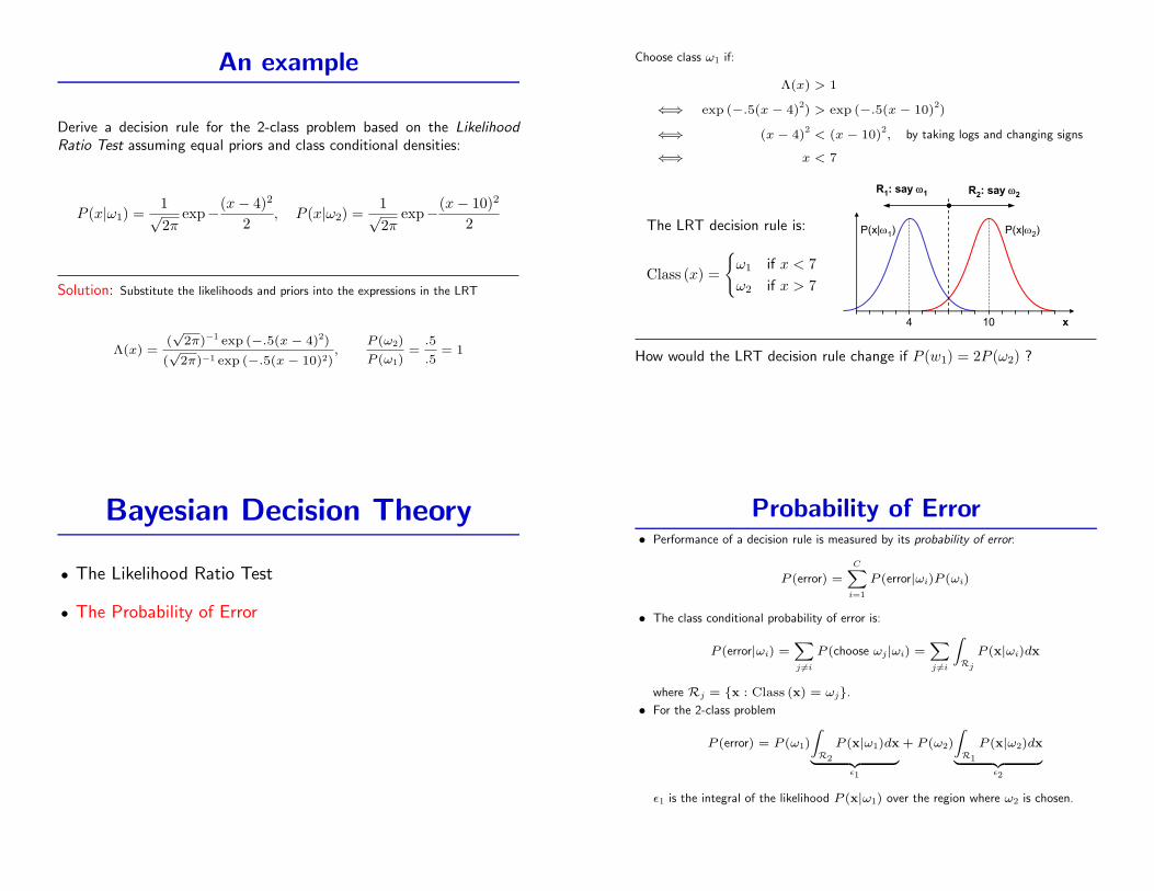
An example

Derive a decision rule for the 2-class problem based on the LikelihoodRatio Test assuming equal priors and class conditional densities:

P (x|ω1) =1√2π

exp−(x− 4)2

2, P (x|ω2) =

1√2π

exp−(x− 10)2

2

Solution: Substitute the likelihoods and priors into the expressions in the LRT

Λ(x) =(√

2π)−1 exp (−.5(x− 4)2)

(√

2π)−1 exp (−.5(x− 10)2),

P (ω2)

P (ω1)=

.5

.5= 1

Choose class ω1 if:

Λ(x) > 1

⇐⇒ exp (−.5(x− 4)2) > exp (−.5(x− 10)

2)

⇐⇒ (x− 4)2

< (x− 10)2, by taking logs and changing signs

⇐⇒ x < 7

The LRT decision rule is:

Class (x) =

{ω1 if x < 7ω2 if x > 7

Introduction to Pattern AnalysisRicardo Gutierrez-OsunaTexas A&M University

3

Likelihood Ratio Test: an example! Given a classification problem with the following class conditional densities,

derive a decision rule based on the Likelihood Ratio Test (assume equal priors)

! Solution" Substituting the given likelihoods and priors into the LRT expression:

" Simplifying the LRT expression:

" Changing signs and taking logs:

" Which yields:

" This LRT result makes sense from an intuitive point of view since the likelihoods are identical and differ only in their mean value

! How would the LRT decision rule change if, say, the priors were such that P(!1)=2P(!2) ?

22 10)(x21

2

4)(x21

1 e2!1)"|P(xe

2!1)"|P(x

""""##

11

e!2

1

e!2

1

)x(#1

2

2

2"

")10x(

21

)4x(21

$%

#""

""

1e

e)x(#1

2

2

2 "

")10x(

21

)4x(21

$%

#""

""

0)10x()4x(1

2

"

"

22

%$

"""

7x1

2

"

"%$

R1: say !1

x

R2: say !2

P(x|!1) P(x|!2)

4 10

How would the LRT decision rule change if P (w1) = 2P (ω2) ?



• The Probability of Error

Probability of Error• Performance of a decision rule is measured by its probability of error:

P (error) =CX

i=1

P (error|ωi)P (ωi)

• The class conditional probability of error is:

P (error|ωi) =Xj 6=i

P (choose ωj|ωi) =Xj 6=i

ZRj

P (x|ωi)dx

where Rj = {x : Class (x) = ωj}.• For the 2-class problem

P (error) = P (ω1)

ZR2

P (x|ω1)dx| {z }ε1

+ P (ω2)

ZR1

P (x|ω2)dx| {z }ε2

ε1 is the integral of the likelihood P (x|ω1) over the region where ω2 is chosen.

Back to the Example

For the decision rule of the previous example, the integrals ε1 and ε2 aredepicted below.

Since we assumed equal priors, thenP (error) = .5(ε1 + ε2)


4

The probability of error (1)! The performance of any decision rule can be measured by its probability of error P[error]

which, making use of the Theorem of total probability (Lecture 2), can be broken up into

! The class conditional probability of error P[error|!i] can be expressed as

! So, for our 2-class problem, the probability of error becomes

" where "i is the integral of the likelihood P(x|!i) over the region Rj where we choose !j

! For the decision rule of the previous example, the integrals "1 and "2 are depicted below" Since we assumed equal priors, then P[error] = ("1 + "2)/2

! Compute the probability for the example above

#$

$C

1iii ]]P[!!|P[errorP[error]

%$$jR

iiji dx)!|x(P]!|!choose[P]!|error[P

!!"!!#$!!"!!#$2

1

1

2

"

R22

"

R11 dx)!|x(P]![Pdx)!|x(P]![P]error[P %% &$

R1: say !1

x

R2: say !2

P(x|!1) P(x|!2)

4 10

"2 "1

Write out the expression for P (error) for this example.

Back to the ExampleFor the decision rule of the previous example, the integrals ε1 and ε2 are depicted below.

Since we assumed equal priors, then

P (error) = .5(ε1 + ε2)


4

The probability of error (1)! The performance of any decision rule can be measured by its probability of error P[error]

which, making use of the Theorem of total probability (Lecture 2), can be broken up into

! The class conditional probability of error P[error|!i] can be expressed as

! So, for our 2-class problem, the probability of error becomes

" where "i is the integral of the likelihood P(x|!i) over the region Rj where we choose !j

! For the decision rule of the previous example, the integrals "1 and "2 are depicted below" Since we assumed equal priors, then P[error] = ("1 + "2)/2

! Compute the probability for the example above

#$

$C

1iii ]]P[!!|P[errorP[error]

%$$jR

iiji dx)!|x(P]!|!choose[P]!|error[P

!!"!!#$!!"!!#$2

1

1

2

"

R22

"

R11 dx)!|x(P]![Pdx)!|x(P]![P]error[P %% &$

R1: say !1

x

R2: say !2

P(x|!1) P(x|!2)

4 10

"2 "1

Write out the expression for P (error) for this example.

ε1 = (2π)−12∫∞

x=7exp(−.5(x− 4)2)dx,

ε2 = (2π)−12∫ 7

x=−∞ exp(−.5(x− 10)2)dx

Probability of Error

Thinking about the 2-class problem, not all decisions are equally good wrtminimizing P (error). For our example consider this (silly) rule:

Class (x) =

{ω1 if x < −100ω2 if x > −100

For this (silly) rule ε1 ∼ 1 and ε2 ∼ 0 which is much more than the errorfor the rule defined by the likelihood ratio test. In fact:

Bayes Error Rate: For any given problem, the minimum probabilityof error is achieved by the Likelihood Ratio Test decision rule. Thisprobability of error is called the Bayes Error Rate and is the BESTany classifier can do.




• Bayes’ Risk

Bayes Risk

• So far have assumed that the penalty of misclassification of a class ω1

example as class ω2 is the same as that for the misclassification of aclass ω2 example as class ω1. But consider misclassifying

– a faulty airplane as a safe airplane (puts people’s lives in danger)

– a safe airplane as a faulty airplane (costs the airline company money)

• Can formalize this concept in terms of a cost function Cij

– Let Cij denote the cost of choosing class ωi when ωj is the true class.

• Bayes’ Risk is the expected value of the cost

E [C] =2X

i=1

2Xj=1

CijP (decide ωi, ωj true class) =2X

i=1

2Xj=1

CijP (x ∈ Ri|ωj)P (ωj)

Bayes RiskWhat is the decision rule that minimizes the Bayes Risk ?

• First note: P (x ∈ Ri|ωj) =∫x∈Ri

P (x|ωj)dx

• Then the Bayes’ Risk is:

E [C] =∫R1

[C11P (ω1)P (x|ω1) + C12P (ω2)P (x|ω2)] dx+∫R2

[C21P (ω1)P (x|ω1) + C22P (ω2)P (x|ω2)] dx

• Now remember∫R1

P (x|ωj)dx +∫R2

P (x|ωj) =∫R1∪R2

P (x|ωj)dx = 1.

E [C] = C11P (ω1)

ZR1

P (x|ω1)dx + C12P (ω2)

ZR1

P (x|ω2)dx +

C21P (ω1)

ZR2

P (x|ω1)dx + C22P (ω2)

ZR2

P (x|ω2)dx+

C21P (ω1)

ZR1

P (x|ω1)dx + C22P (ω2)

ZR1

P (x|ω2)dx + ← +A

−C21P (ω1)

ZR1

P (x|ω1)dx− C22P (ω2)

ZR1

P (x|ω2)dx ← −A

= C21P (ω1)

ZR1∪R2

P (x|ω1)dx + C22P (ω2)

ZR1∪R2

P (x|ω2)dx +

(C12 − C22)P (ω2)

ZR1

P (x|ω2)dx− (C21 − C11)P (ω1)

ZR1

P (x|ω1)dx

= C21P (ω1) + C22P (ω2) +

(C12 − C22)P (ω2)

ZR1

P (x|ω2)dx− (C21 − C11)P (ω1)

ZR1

P (x|ω1)dx

We want to find the region R1 that minimizes the Bayes’ Risk. From theprevious slide we see the first two terms of E [C] are constant with respectto R1. Thus the optimal region is:

R∗1 = arg minR1

(ZR1

[(C12 − C22)P (ω2)P (x|ω2)− (C21 − C11)P (ω1)P (x|ω1)] dx

)

= arg minR1

(ZR1

g(x)dx

)

Note we are assuming C21 > C11 and C12 > C22, that is the cost of amisclassification is higher than the cost of a correct classification. Thus:

(C12 − C22) > 0 AND (C21 − C11) > 0

Bayes Risk (2)

• Temporally forget about the specific expression of g(x). Consider thetype of decision region R∗1 we are looking for. Select the intervals thatminimize the integral

∫R1

g(x)dx, that is the intervals where g(x) < 0

• Thus we will choose R∗1 such that

(C21 − C11)P (ω1)P (x|ω1) > (C12 − C22)P (ω2)P (x|ω2)

Rearranging the terms yields:

P (x|ω1)P (x|ω2)

>(C12 − C22)P (ω2)(C21 − C11)P (ω1)

Therefore we obtain the decision rule

A Likelihood Ratio Test:

Class (x) =

ω1 if P (x|ω1)

P (x|ω2)> (C12−C22)P (ω2)

(C21−C11)P (ω1)

ω2 if P (x|ω1)P (x|ω2)

< (C12−C22)P (ω2)(C21−C11)P (ω1)

Bayes Risk: An ExampleConsider the following 2 class classification problem. The likelihoodfunctions for each class are:

P (x|ω1) = (2π3)−12 exp

(−.5x2/3

), P (x|ω2) = (2π)−

12 exp

(−.5(x− 2)2

)


9

-6 -4 -2 0 2 4 60

0.02

0.04

0.06

0.08

0.1

0.12

0.14

0.16

0.18

0.2

x

-6 -4 -2 0 2 4 60

0.02

0.04

0.06

0.08

0.1

0.12

0.14

0.16

0.18

0.2

x

likel

ihoo

d

The Bayes Risk: an example! Consider a classification problem with two classes

defined by the following likelihood functions

" Sketch the two densities" What is the likelihood ratio?" Assume P[!1]=P[!2]=0.5, C11=C22=0, C12=1 and C21=31/2.

Determine a decision rule that minimizes the probability of error

2

2

2)(x21

2

3x

21

1

e2!1)"|P(x

e32!

1)"|P(x

""

"

#

#

27.1,73.4x012x12x2

0)2x(21

3x

21

1e

e

31

e!2

1

e3!2

1

)x(#

1

2

1

2

1

2

2

2

1

2

2

2

"

"

2

"

"

22

"

")2x(

21

3x

21

"

")2x(

21

3x

21

#$%&

'"

%&

"'"

%&

%&

#

""

"

""

"

R1R2R1

The priors are: P (ω1) = P (ω2) = .5

Define the (mis)classification costsas: C11 = C22 = 0, C12 = 1, C21 =√

3

Problem: Determine a decision rule minimizing the probability of error.

Bayes Risk: An Example (2)

Solution: Λ(x) =(2π3)

−12 exp

“−.5x2/3

”(2π)−1

2 exp (−.5(x−2)2)=

(3)−1

2 exp“−.5x2/3

”exp (−.5(x−2)2)

.

Choose class ω1 if Λ(x) >.5(1− 0)

.5(√

3− 0)

⇐⇒(3)−

12 exp

`−.5x2/3

´exp (−.5(x− 2)2)

> 1

⇐⇒ exp“−.5x

2/3”

> exp“−.5(x− 2)

2”

⇐⇒ −1

2

x2

3>

1

2(x− 2)

2

⇐⇒ x2 − 6x + 6 > 0

⇐⇒ x > 4.73 and x < 1.27Introduction to Pattern AnalysisRicardo Gutierrez-OsunaTexas A&M University

9

-6 -4 -2 0 2 4 60

0.02

0.04

0.06

0.08

0.1

0.12

0.14

0.16

0.18

0.2

x

-6 -4 -2 0 2 4 60

0.02

0.04

0.06

0.08

0.1

0.12

0.14

0.16

0.18

0.2

x

likel

ihoo

d

The Bayes Risk: an example! Consider a classification problem with two classes

defined by the following likelihood functions

" Sketch the two densities" What is the likelihood ratio?" Assume P[!1]=P[!2]=0.5, C11=C22=0, C12=1 and C21=31/2.

Determine a decision rule that minimizes the probability of error

2

2

2)(x21

2

3x

21

1

e2!1)"|P(x

e32!

1)"|P(x

""

"

#

#

27.1,73.4x012x12x2

0)2x(21

3x

21

1e

e

31

e!2

1

e3!2

1

)x(#

1

2

1

2

1

2

2

2

1

2

2

2

"

"

2

"

"

22

"

")2x(

21

3x

21

"

")2x(

21

3x

21

#$%&

'"

%&

"'"

%&

%&

#

""

"

""

"

R1R2R1




• Bayes’ Risk

• Bayes, MAP and ML Criteria

Variations of the LRT

• The LRT decision rule minimizing the Bayes Risk is also known as theBayes Criterion

Bayes Criterion→ Class (x) =

8<:ω1 if Λ(x) >(C12−C22)P (ω2)

(C21−C11)P (ω1)

ω2 if Λ(x) <(C12−C22)P (ω2)

(C21−C11)P (ω1)

• Minimize the probability of error, that is the Bayes Criterion withCij = δij, this version of the LRT decision is referred to as theMaximum A Posteriori Criterion.

MAP Criterion→ Class (x) =

(ω1 if P (ω1|x) > P (ω2|x)

ω2 if P (ω1|x) < P (ω2|x)

• Finally, for the case of equal priors P (ωi) and Cij = δij (a zero onecost function) the LRT decision rule is called the Maximum LikelihoodCriterion, since it will minimize the likelihood P (x|ωi).

ML Criterion→ Class (x) =

(ω1 if P (x|ω1) > P (x|ω2)

ω2 if P (x|ω1) < P (x|ω2)

Variations of the LRT (2)

Two more decision rules are commonly cited in the related literature.

• The Neyman-Pearson Criterion which also leads to a LRT decision rule.It fixes one class error probability, say ε < α and seeks to minimize theother.

• The Minimax Criterion, derived from the Bayes Criterion and seeks tominimize the maximum Bayes Risk.




• Bayes’ Risk


• Multi-class functions

Decision rules for multi-class problemsThe decision rule minimizing P (error) generalizes to multi-class problems.

• The derivation is easier if we express P (error) in terms of making a correct assignment.

P (error) = 1− P (correct)

• Probability of making a correct assignment is

P (correct) =CX

i=1

P (ωi)

ZRi

P (x|ωi)dx

=CX

i=1

ZRi

P (x|ωi)P (ωi)dx

=CX

i=1

ZRi

P (ωi|x)P (x)dx| {z }Ti

• The problem of minimizing P (error) is equivalent to that of maximizingP (correct).

• To maximize P (correct) we have to maximize each of the integrals Ti.In turn, each integral Ti will be maximized by choosing the class ωi

that yields the maximum P (ωi|x) =⇒ we will define Ri to be theregions where P (ωi|x) is maximum.


12

Minimum P[error] rule for multi-class problems! The decision rule that minimizes P[error] generalizes very easily to multi-class

problems" For clarity in the derivation, the probability of error is better expressed in terms of the

probability of making a correct assignment

" The probability of making a correct assignment is

" The problem of minimizing P[error] is equivalent to that of maximizing P[correct]. Expressing P[correct] in terms of the posteriors:

" In order to maximize P[correct], we will have to maximize each of the integrals !i. In turn, each integral !i will be maximized by choosing the class "i that yields the maximum P["i|x] # we will define Ri to be the region where P["i|x] is maximum

! Therefore, the decision rule that minimizes P[error] is the MAP Criterion

]correct[P1]error[P $%

& '%

%C

1ii

Ri dx)!|x(P)!(P]correct[P

i

&'& '& '%

!

%%

%%%C

1i Ri

C

1iii

R

C

1ii

Ri

i

iii

P(x)dxx)|P(!)dx)P(!!|P(x)dx!|P(x)P(!P[correct]!! "!! #$

x

Pro

babi

lity

R2 R1 R3 R2 R1

P("1|x)P("2|x)

P("3|x)

Therefore, the decision rule that minimizes P (error) is the MAP Criterion.

Minimum Bayes Risk

• Define the overall decision rule as a function

α : x → {α1, α2, · · · , αC} s.t. α(x) = αi if x is assigned to class ωi.

• The risk R(α(x)|x) of assigning x to class α(x) = αi is

R(αi|x) =C∑

j=1

CijP (ωj|x)

• The Bayes Risk associate with the decision rule α(x) is

R(α(x)) =∫

R(α(x)|x)P (x)dx

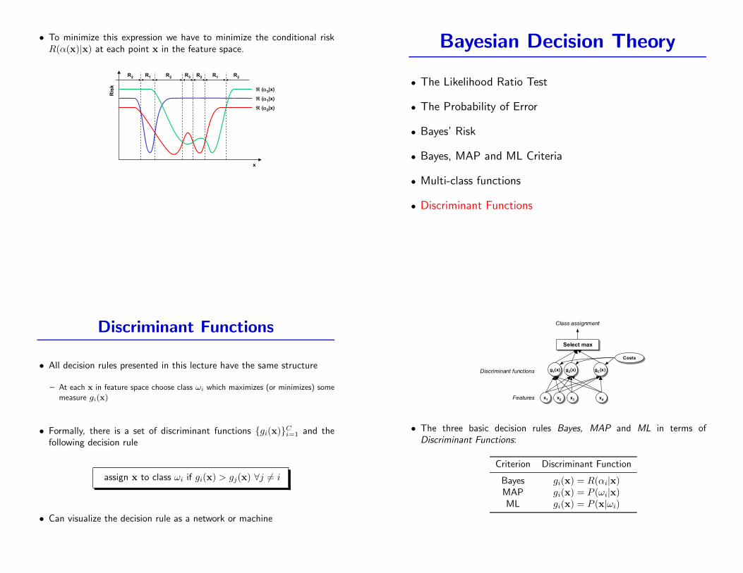
• To minimize this expression we have to minimize the conditional riskR(α(x)|x) at each point x in the feature space.


13

Minimum Bayes Risk for multi-class problems ! To determine which decision rule yields the minimum Bayes Risk for the multi-class

problem we will use a slightly different formulation" We will denote by !i the decision to choose class "i, " We will denote by !(x) the overall decision rule that maps features x into classes "i: !(x)#{!1 , !2 , …, !C}

! The (conditional) risk $(!i|x) of assigning a feature x to class "i is

! And the Bayes Risk associated with the decision rule !(x) is

! In order to minimize this expression,we will have to minimize the conditional risk $(!(x)|x) at each point x in the feature space, which in turn is equivalent to choosing "i such that $(!i|x) is minimum

% & % & '(

($(#$C

1jjijii )x|!(PCx|"")x("

% & % & dx)x(Px|)x(")x(" )$($

x

Ris

k

R1 R2 R3 R2R1R2R2

$ (!2|x)

$ (!3|x)

$ (!1|x)




• Bayes’ Risk


• Multi-class functions

• Discriminant Functions

Discriminant Functions

• All decision rules presented in this lecture have the same structure

– At each x in feature space choose class ωi which maximizes (or minimizes) some

measure gi(x)

• Formally, there is a set of discriminant functions {gi(x)}Ci=1 and the

following decision rule

assign x to class ωi if gi(x) > gj(x) ∀j 6= i

• Can visualize the decision rule as a network or machine


14

Discriminant functions! All the decision rules we have presented in this lecture have the same structure

" At each point x in feature space choose class !i which maximizes (or minimizes) some measure gi(x)! This structure can be formalized with a set of discriminant functions gi(x), i=1..C, and the

following decision rule

! Therefore, we can visualize the decision rule as a network or machine that computes C discriminant functions and selects the category corresponding to the largest discriminant. Such network is depicted in the following figure (presented already in Lecture 1)

! Finally, we express the three basic decision rules: Bayes, MAP and ML in terms of Discriminant Functions to show the generality of this formulation

i"j(x)g(x)gif!classtoxassign" jii "#$

x2x2 x3

x3 xdxd

g1(x)g1(x)

x1x1

g2(x)g2(x) gC(x)gC(x)

Select maxSelect max

CostsCosts

Class assignment

Discriminant functions

Features

Criterion Discriminant FunctionBayes gi(x)=-%(&i|x)MAP gi(x)=P(!i|x)ML gi(x)=P(x|!i)

• The three basic decision rules Bayes, MAP and ML in terms ofDiscriminant Functions:

Criterion Discriminant Function

Bayes gi(x) = R(αi|x)MAP gi(x) = P (ωi|x)ML gi(x) = P (x|ωi)

Discriminant Functions for the class ofGaussian Distributions

Quadratic Classifiers

• Bayes classifiers for Normally distributed classes

Bayes classifiers for Normally distributed classes

• The (MAP) decision rule minimizing the probability of error can beformulated as a family of discriminant functions

Choose class ωi if gi(x) > gj(x) ∀i 6= j with gi(x) = P (ωi|x)

For classes that are normally distributed, this family can be reduced to very simple

expressions.

• General expression for Gaussian densities

– The multi-variate Normal density is defined as

fX(x) =1

(2π)n2 |Σ|

12

exp

„−

1

2(x− µ)

TΣ−1

(x− µ)

«

– Using Bayes’ rule the MAP discriminant function becomes

gi(x) =P (x|ωi)P (ωi)

P (x)

=1

(2π)n2 |Σi|

12

exp

„−

1

2(x− µi)

TΣ−1i (x− µi)

«P (ωi)

P (x)

– Eliminating constant terms

gi(x) = |Σi|−1/2exp

„−

1

2(x− µ)

TΣ−1i (x− µ)

«P (ωi)

– Taking the log since it is a monotonically increasing function

gi(x) = −12(x− µi)

TΣ−1i (x− µi)− 1

2 log (|Σi|) + log (P (ωi))

Quadratic Discriminant Function



– Case 1: Σi = σ2I

Case 1: Σi = σ2I

• The features are statistically independent with the same variance forall classes.

– The quadratic function becomes

gi(x) = −1

2(x− µi)

T(σ

2I)−1

(x− µi)−1

2log (|σ2

I|) + log (P (ωi))

= −1

2σ2(x− µi)

T(x− µi)−

N

2log (σ

2) + log (P (ωi))

= −1

2σ2(x− µi)

T(x− µi) + log (P (ωi)), dropping the second term

= −1

2σ2(xTx− 2µ

Ti x + µ

Ti µi) + log (P (ωi))

– Eliminate the term xTx as it is constant for all classes. Then

gi(x) = −1

2σ2(−2µ

Ti x + µ

Ti µi) + log (P (ωi))

= wTi x + wi0

where

wi =µi

σ2and wi0 = −

1

2σ2µ

Ti µi + log (P (ωi))

– As the discriminant is linear, the decision boundaries gi(x) = gj(x) will be

hyper-planes.

• If we assume equal priors (also know as the nearest mean classifier)

Minimum distance classifier: gi(x) = − 12σ2(x− µi)T (x− µi)

• Properties of the class-conditional probabilities

– the loci of constant probability for each class are hyper-spheres

Case 1: Σi = σ2I

• The decision boundaries are the hyperplanes gi(x) = gj(x), and canbe written as

w̃T (x− x0) = 0, after some algebra

where

w̃ = µi − µj

x0 =12(µi + µj)−

σ2

‖µi − µj‖2ln

P (ωi)P (ωj)

(µi − µj).

• The hyperplane separating Ri and Rj passes through the point x0 andis orthogonal to the vector w̃.

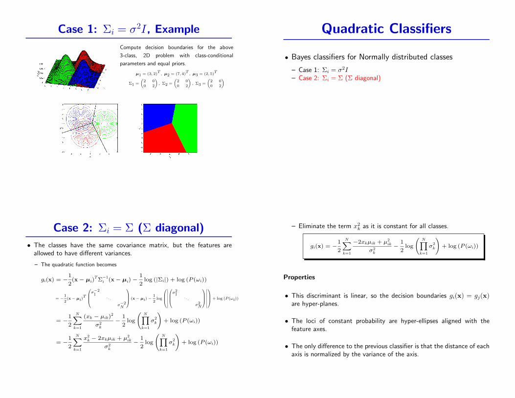
Case 1: Σi = σ2I, Example


4

Case 1: !i="2I, example! To illustrate the previous result, we will

compute the decision boundaries for a 3-class, 2-dimensional problem with the following class mean vectors and covariance matrices and equal priors

# $ # $ # $

%&

'()

*+%

&

'()

*+%

&

'()

*+

+++

2002

!2002

!2002

!

52µ47µ23µ

321

T3

T2

T1

Compute decision boundaries for the above

3-class, 2D problem with class-conditional

parameters and equal priors.

µ1 = (3, 2)T

, µ2 = (7, 4)T

, µ3 = (2, 5)T

Σ1 =

„2 00 2

«, Σ2 =

„2 00 2

«, Σ3 =

„2 00 2

«


4

Case 1: !i="2I, example! To illustrate the previous result, we will

compute the decision boundaries for a 3-class, 2-dimensional problem with the following class mean vectors and covariance matrices and equal priors

# $ # $ # $

%&

'()

*+%

&

'()

*+%

&

'()

*+

+++

2002

!2002

!2002

!

52µ47µ23µ

321

T3

T2

T1



– Case 1: Σi = σ2I– Case 2: Σi = Σ (Σ diagonal)

Case 2: Σi = Σ (Σ diagonal)

• The classes have the same covariance matrix, but the features areallowed to have different variances.

– The quadratic function becomes

gi(x) = −1

2(x− µi)

TΣ−1i (x− µi)−

1

2log (|Σi|) + log (P (ωi))

= −1

2(x− µi)

T

0BB@σ−21

. . .

σ−2N

1CCA (x− µi)−1

2log

0BB@˛̨̨̨˛̨̨̨0BB@

σ21

. . .

σ2N

1CCA˛̨̨̨˛̨̨̨1CCA+ log (P (ωi))

= −1

2

NXk=1

(xk − µik)2

σ2k

−1

2log

NY

k=1

σ2k

!+ log (P (ωi))

= −1

2

NXk=1

x2k − 2xkµik + µ2

ik

σ2k

−1

2log

NY

k=1

σ2k

!+ log (P (ωi))

– Eliminate the term x2k as it is constant for all classes.

gi(x) = −1

2

NXk=1

−2xkµik + µ2ik

σ2k

−1

2log

NY

k=1

σ2k

!+ log (P (ωi))

Properties

• This discriminant is linear, so the decision boundaries gi(x) = gj(x)are hyper-planes.

• The loci of constant probability are hyper-ellipses aligned with thefeature axes.

• The only difference to the previous classifier is that the distance of eachaxis is normalized by the variance of the axis.

Case 2: Σi = Σ (Σ diagonal), example


6

! To illustrate the previous result, we will compute the decision boundaries for a 3-class, 2-dimensional problem with the following class mean vectors and covariance matrices and equal priors

! " ! " ! "

#$

%&'

()#

$

%&'

()#

$

%&'

()

)))

2001

!2001

!2001

!

52µ45µ23µ

321

T3

T2

T1

Case 2: *i= * (* diagonal), exampleCompute decision boundaries for the above



µ1 = (3, 2)T

, µ2 = (5, 4)T

, µ3 = (2, 5)T

Σ1 =

„1 00 2

«, Σ2 =

„1 00 2

«, Σ3 =

„1 00 2

«


6


! " ! " ! "

#$

%&'

()#

$

%&'

()#

$

%&'

()

)))

2001

!2001

!2001

!

52µ45µ23µ

321

T3

T2

T1

Case 2: *i= * (* diagonal), example Quadratic Classifiers


– Case 1: Σi = σ2I– Case 2: Σi = Σ (Σ diagonal)– Case 3: Σi = Σ (Σ non-diagonal)

Case 3: Σi = Σ (Σ non-diagonal)• All classes have the same covariance matrix, but it is not necessarily

diagonal.

• The quadratic discriminant function becomes

gi(x) = −1

2(x− µi)


1


= −1

2(x− µi)

TΣ−1

(x− µi)−1

2log (|Σ|) + log (P (ωi))

• Eliminate the term log (|Σ|), which is constant for all classes.

gi(x) = −12(x− µi)

TΣ−1(x− µi) + log (P (ωi))

• The quadratic term is called the Mahalanobis distance, a very importantterm in Statistical PR.

Mahalanobis distance: ‖x− y‖2Σ−1 = (x− y)TΣ−1(x− y)

• The Mahalanobis distance is a vector distance that uses a Σ−1 norm.

– Σ−1 can be thought as a stretching factor on the space.

– For Σ = I the Mahalanobis distance becomes the Euclidean distance.


7

Case 3: !i=! (! non-diagonal)! In this case, all the classes have the same covariance matrix, but this is no longer diagonal! The quadratic discriminant becomes

! Eliminating the term log|"|, which is constant for all classes

" The quadratic term is called the Mahalanobis distance, a very important distance in Statistical PR

! The Mahalanobis distance is a vector distance that uses a "-1 norm

" "-1 can be thought of as a stretching factor on the space" Note that for an identity covariance matrix ("=I), the

Mahalanobis distance becomes the familiar Euclidean distance

# $ # $

# $ # $)!P(loglog21-)µ(x)µ(x

21

)!P(loglog21-)µ(x)µ(x

21(x)g

ii1T

i

iii1

iT

ii

%"&"&&'

'%"&"&&'

&

&

# $)!P(log)µ(x)µ(x21(x)g ii

1i

Tii %&"&&' &

(x2

x1

" µ-x 2i '

K µ-x 2i 1 '&"

y)(xy)(xy-x 1T21 &"&' &

"&

DistancesMahalanobi

Case 3: Σi = Σ (Σ non-diagonal)

• Expansion of the quadratic term in the discriminant yields

gi(x) = −1

2(x− µi)

TΣ−1

(x− µi) + log (P (ωi))

= −1

2

“xT

Σ−1x− 2µ

Ti Σ−1x + µ

Ti Σ−1

µi

”+ log (P (ωi))

• Removing the term xTΣ−1x which is constant for all classes

gi(x) = −1

2

“−2µ

Ti Σ−1x + µ

Ti Σ−1

µi

”+ log (P (ωi))

• Reorganizing terms get:

gi(x) = wTi x + wi0 with wi = Σ

−1µi and wi0 = −

1

2µ

Ti Σ−1

µi + log (P (ωi))

Properties

• The discriminant is linear, so the decision boundaries are hyper-planes.

• The constant probability loci are hyper-ellipses aligned with theeigenvectors of Σ.

• If we can assume equal priors the classifier becomes a minimum(Mahalanobis) distance classifier.

Equal Priors: gi(x) = −12(x− µi)TΣ−1(x− µi)

Case 3: Example


9


! " ! " ! "

#$

%&'

()#

$

%&'

()#

$

%&'

()

)))

27.07.01

!27.07.01

!27.07.01

!

52µ45µ23µ

321

T3

T2

T1

Case 3: *i=* (* non-diagonal), exampleCompute decision boundaries for the above



µ1 = (3, 2)T

, µ2 = (5, 4)T

, µ3 = (2, 5)T

Σ1 =

„.5 .7.7 2

«, Σ2 =

„1 .7.7 2

«, Σ3 =

„1 .7.7 2

«


9


! " ! " ! "

#$

%&'

()#

$

%&'

()#

$

%&'

()

)))

27.07.01

!27.07.01

!27.07.01

!

52µ45µ23µ

321

T3

T2

T1

Case 3: *i=* (* non-diagonal), exampleQuadratic Classifiers


– Case 1: Σi = σ2I– Case 2: Σi = Σ (Σ diagonal)– Case 3: Σi = Σ (Σ non-diagonal)– Case 4: Σi = σ2

i I

Case 4: Σi = σ2i I

• Each class has a different covariance matrix, which is proportional tothe identity matrix.

– The quadratic discriminant becomes

gi(x) = −1

2(x− µi)


1


= −1

2(x− µi)

Tσ−2i (x− µi)−

N

2log“

σ2i

”+ log (P (ωi))

• The expression cannot be reduce further so

– The decision boundaries are quadratic: hyper-ellipses

– The loci of constant probability are hyper-spheres aligned with the feature axis.

Case 4: Σi = σ2i I, example

Compute decision boundaries for the above


parameters.

µ1 = (3, 2)T

, µ2 = (5, 4)T

, µ3 = (2, 5)T

Σ1 =

„.5 00 .5

«, Σ2 =

„1 00 1

«, Σ3 =

„2 00 2

«




i I– Case 5: Σi 6= Σj, General Case

Case 5: Σi 6= Σj, General Case

• Have already derived the expression for the general case it is:

gi(x) = −1

2(x− µi)


1


– Reorganizing terms in a quadratic form yields

gi(x) = xTWix + wTi x + wi0

where

Wi = −12Σ−1

i ,

wi = Σ−1i µi,

wi0 = −12µT

i Σ−1i µi −

12

log (|Σi|) + log (P (ωi))

Properties

• The loci of constant probability for each class are hyper-ellipses, orientedwith the eigenvectors of Σi for that class.

• The decision boundaries are quadratic: hyper-ellipses or hyper-parabolloids

• The quadratic expression in the discriminant is proportional to theMahalanobis distance using the class-conditional variance Σi.

Case 5: Σi 6= Σj, Example


13


! " ! " ! "

#$

%&'

()#

$

%&'

(*

*)#

$

%&'

(*

*)

)))

35.05.05.0

!7111

!2111

!

52µ45µ23µ

321

T3

T2

T1

Case 5: +i,+j general case, example

Zoomout

Compute the decision boundaries for the above3-class, 2-dimensional problem with class-conditional parameters.

µ1 = (3, 2)T

µ2 = (5, 4)T

µ3 = (2, 5)T

Σ1 =

„1 −1−1 2

«, Σ2 =

„1 00 1

«, Σ3 =

„2 00 2

«


13


! " ! " ! "

#$

%&'

()#

$

%&'

(*

*)#

$

%&'

(*

*)

)))

35.05.05.0

!7111

!2111

!

52µ45µ23µ

321

T3

T2

T1

Case 5: +i,+j general case, example

Zoomout





• Numerical Example

Numerical Example

Derive the discriminant function for the 2-class 3D classification problem defined by the

following Gaussian Likelihoods

µ1 =

0@0

0

0

1A ; µ2 =

0@1

1

1

1A ; Σ1 = Σ2 =

0@14 0 0

0 14 0

0 0 14

1A ; P (ω2) = 2P (ω1)

Solution:

g1(x) =1

2σ2(x− µ1)

T(x− µ1) + log (P (ω1))

= −1

2(14)

(x1 − 0, x2 − 0, x3 − 0)

0@x1 − 0

x2 − 0

x3 − 0

1A+ log

„1

3

«

g2(x) = −1

2(14)

(x1 − 1, x2 − 1, x3 − 1)

0@x1 − 1

x2 − 1

x3 − 1

1A+ log

„2

3

«

Classify x as ω1 if g1(x) > g2(x).

g1(x) > g2(x)

⇐⇒ − 2(xTx) + log

„1

3

«> −2((x1 − 1)

2+ (x2 − 1)

2+ (x3 − 1)

2) + log

„2

3

«⇐⇒ x1 + x2 + x3 <

6− log 2

4= 1.32

Therefore the decision rule is:

Class (x) =

(ω1 if x1 + x2 + x3 < 1.32

ω2 if x1 + x2 + x3 > 1.32

Classify the test example xu = (.1, .7, .8)T

.1 + .7 + .8 = 1.6 > 1.32 =⇒ xu ∈ ω2





• Numerical Example

• Conclusions

Conclusions

• We can draw the following conclusions

– The Bayes classifier for normally distributed classes (general case) is a quadratic

classifier.

– The Bayes classifier for normally distributed classes with equal covariance matrices

is a linear classifier.

– The minimum Mahalanobis distance classifier is Bayes-optimal for

∗ normally distributed classes and

∗ equal covariance matrices and

∗ equal priors

– The minimum Euclidean distance classifier is Bayes-optimal for

∗ normally distributed classes and

∗ equal covariance matrices proportional to the identity matrix and

∗ equal priors

– Both Euclidean and Mahalanobis distance classifiers are linear classifiers.

• Some of the most popular classifiers can be derived from decision-

theoretic principles and some simplifying assumptions.

– Using a specific (Euclidean or Mahalanobis) minimum distance classifier implicitly

corresponds to certain statistical assumptions.

– Can rarely answer the question if these assumptions hold for real problems. In

most cases limited to answering “Does this classifier solve our problem or not? ”

lecture 5 bayesian decision theory likelihood ratio test · lecture 5 bayesian decision theory { a...

Documents