The Pennsylvania State University

APPLIED RESEARCH LABORATORY Post Office Box 30

State College, P A 16804

Modal Analysis Using the Singular Value Decomposition

by

J. B. Fahnline, R. L. Campbell, and S. A. Hambric

Technical Report 04-008 May 2004

E. G. Liszka, Director Applied Research Laboratory

Approved for public release, distribution unlimited

REPORT DOCUMENTATION PAGE Form Approved OMB No. 0704-0188

The public reporting burden for this collection of information is estimated to average 1 hour per response, including the time for reviewing instructions, searching existing data sources, gathering and maintaining the data needed, and completing and reviewing the collection of information. Send comments regarding this burden estimate or any other aspect of this collection of information, Including sug�estions for reducing the burden, to Department of Defense, Washington Headquarters Services, Directorate for Information Operations and Reports (07()4.0188), 1216 Jefferson avis Highway, Suite 1204, Arlington, VA 22202-4302. Respondents should be aware that notwithstanding any other provision of law, no person shall be subject to any penalty for failing to comply with a collection of information if it does not display a currently valid OMB control number.

PLEASE DO NOT RETURN YOUR FORM TO THE ABOVE ADDRESS.

1. REPORT DATE (DD-MM-YYYYJ , 2. REPORT TYPE

May 2004 Technical Report

4. TITLE AND SUBTITLE

Modal Analysis Using the Singular Value Decomposition

6. AUTHORISI

J. B. Fahnline, R. L. Campbell, and S. A. Hambirc

7. PERFORMING ORGANIZATION NAMEISI AND ADDRESS(ESI

Applied Research L aboratory Post Office Box 30 State College, PA 16804

9. SPONSORING/MONITORING AGENCY NAME(S) AND ADDRESS(ES)

12. DISTRIBUTION/AVAILABILITY STATEMENT

Approved for public release. Distribution unlimited

13. SUPPLEMENTARY NOTES

14. ABSTRACT

SEE ATIACHED.

15. SUBJECT TERMS

16. SECURITY CLASSIFICATION OF: 17. LIMITATION OF 18. NUMBER

a. REPORT b. ABSTRACT c. THIS PAGE ABSTRACT OF

PAGES

Unclassified Unclassified Unclassified Unclassified Unlimited- UU

21

2

3. DATES COVERED (From - To)

5a. CONTRACT NUMBER

PL01000100

5b. GRANT NUMBER

5c. PROGRAM ELEMENT NUMBER

5d. PROJECT NUMBER

5e. TASK NUMBER

5f. WORK UNIT NUMBER

8. PERFORMING ORGANIZATION

REPORT NUMBER

TR04-008

10. SPONSOR/MONITOR'S ACRONYM(S)

11. SPONSOR/MONITOR'S REPORT

NUMBER(S)

19a. NAME OF RESPONSIBLE PERSON

19b. TELEPHONE NUMBER (Include area code!

Standard Form 298 (Rev. 8/98) Prescribed by ANSI Std. Z39. 18

Abstract:

Many methods exist for identifying modal parameters from experimental transfer function measurements. For frequency domain calculations, rational fraction polynomials have become the method of choice, although it generally requires the user to identify frequency bands of interest along with the number of modes in each band. This process can be tedious, especially for systems with a large number of modes, and it assumes the user can accurately assess the number of modes present in each band from frequency response plots of the transfer functions. When the modal density is high, better results can be obtained by using the singular value decomposition to help separate the modes before the modal identification process begins. In a typical calculation, the transfer function data for a single frequency is arranged in matrix form with each column representing a different drive point. The matrix is input to the singular value decomposition algorithm and left- and right-singular vectors and a diagonal singular value matrix are computed. The calculation is repeated at each analysis frequency and the resulting data is used to identify the modal parameters. In the optimal situation, the singular value decomposition will completely separate the modes from each other, so that a single transfer function is produced for each mode with no residual effects. A graphical method has been developed to simplify the process of identifying the modes, yielding a relatively simple method for computing mode shapes and resonance frequencies from experimental data.

3

TABLE OF CONTENTS

Page Number

ABSTRACT .............................................................................................................. .

LIST OF TABLES .................................................................................................... .

LIST OF FIGURES .................................................................................................. .

IN"TRODUCTION .................................................................................................... .

A. Finding the Resonances ................................................................................ .

B.

C.

D.

E.

Modal Parameter Identification ........... ................. ........................................ .

Testing the Algorithm ................................................................................... .

Step-by-Step Analysis Procedure ................................................................. .

Future Work .................................................................................................. .

3 5 5 6 6 10 11 12 12

REFERENCES .......................................................................................................... 13 APPENDIX ................................................ ............................................................... 20

4

LIST OF TABLES Table Number Title Page Number

1 Comparison of various methods for computing resonance frequencies and damping loss factors ................................................. . 14

LIST OF FIGURES

Figure Number Title Page Number

1 Singular values as a function of frequency for a series of closely-spaced modes ...................................................................................... . 15

2 Modal transfer functions overlaid on the singular values as a function of frequency ......................................................................... . 16

3 Circle fits for two overlapping modes using modal transfer functions .......................... ........ ........................................................... . 17

4 Input to, and output from, the Savitz-Golay smoothing filter ............ . 18 5 Original circle fit and circle fit after subtracting residual terms

and rotating ......................................................................................... . 19

5

INTRODUCTION

Many methods exist for identifying modal parameters from experimental transfer function measurements. For frequency domain calculations, rational fraction polynomials 1 have become the method of choice, although it generally requires the user to identify frequency bands of interest along with the number of modes in each band. This process can be tedious, especially for systems with a large number of modes, and it assumes the user can accurately assess the number of modes present in each band from frequency response plots of the transfer functions.

When the modal density is high, better results can be obtained by using the singular value decomposition to help separate the modes before the modal identification process begins 2,3. In a typical calculation, the transfer function data for a single frequency is arranged in matrix form with each column representing a different drive point. The matrix is input to the singular value decomposition algorithm and left- and right-singular vectors and a diagonal singular value matrix are computed. The calculation is repeated at each analysis frequency and the resulting data is used to identify the modal parameters. In the optimal situation, the singular value decomposition will completely separate the modes from each other, so that a single transfer function is produced for each mode with no residual effects.

In practice, the modal transfer functions are never completely free from residual effects of nearby modes, but the resonance frequencies and damping loss factors can be accurately identified using simple one-degree-of-freedom models nonetheless. As an example, Figure 1 shows a plot of the singular values as a function of frequency for a typical case. Because the singular values are computed and output in order of descending magnitude, a single curve on the plot does not track a single mode. For example, just below 55 Hz, the top two curves switch the modes that they're tracking. However, by using the singular value decomposition at one frequency to decompose the coefficient matrix at nearby frequencies, it is possible to force the singular values to track only a single mode. The resulting functions were originally called "enhanced frequency response functions" 2, although we prefer the more descriptive name "modal transfer functions". Figure 2 shows the modal transfer functions, as indicated by the thicker curves, overlaid on the original singular value plot from Figure 1. The curves are cut-off because the modal transfer functions are only calculated for a limited number of frequencies on either side of the peak to reduce the computational expense.

Once the modal transfer functions have been calculated, all that remains is to identify peaks in the response and calculate the modal parameters. To demonstrate that it should be possible to identify modal parameters from the modal transfer function data using SDOF (single-degree-of­freedom) methods, Figure 3 shows Nyquist plots of the resulting modal circles for the two overlapping modes at 69.0 and 70.3 Hz. We will give a complete derivation of the algorithm for identifying the modal parameters in the next section. For now, we will only say that that the data resembles a transfer function for a single-degree-of-freedom system.

A. Finding the Resonances

Because it is easy to search a string of numbers for a peak, it may not seem like the process of identifying modal peaks should be especially difficult. However, it is undoubtedly the most

6

difficult part of the modal identification process. The basic problem is that noise is always present in the transfer function measurements, even for carefully controlled experiments. Also, the frequency resolution for the resonance peaks changes depending on the damping levels and location of the peak within the spectrum. For example, resonance peaks at the lower end of the frequency spectrum often have low damping and are not sufficiently resolved in frequency while peaks at the higher end of the spectrum typically have larger damping levels and are overly resolved. This is primarily a consequence of the uniform frequency-spacing required by the FFT algorithms. It might be possible to use phase information for the transfer function data to help in finding the modes, but in practice the phase information generally has higher noise levels than the transfer function magnitudes. One way to avoid this difficulty is to require the user to identify the locations of the modes by hand, usually with some sort of graphical interface, which is both tedious and time consuming. In our implementation, we have tried to reduce the user-input requirements by dividing the process into two stages. In the first stage, an automatic mode finding routine is executed. The routine has been designed with rather loose requirements so that it does not exclude valid modes. Consequently, the routine inevitably finds a number of extraneous modes. In the second stage, an interactive MATLAB-based program is used to edit out the extraneous peaks based on user input. A balance is thus struck between the accuracy of the mode finding algorithm and the amount of user input required. Hopefully, in the future the algorithm can be refined, thus eliminating more of the extraneous peaks and making the process less reliant on the user's subjective judgment.

In the mode finding algorithm, a number of enhancements have been implemented to make the process somewhat immune to noise. The first and most important way to reduce noise levels is to pass the data through the SVD algorithm. The output from the singular value decomposition consists of three matrices U, V, and S. The U and V matrices are unitary (i.e. U UH = 1, where the superscript H indicates a Hermitian transpose), and the S matrix contains the singular values on its diagonal and is real-valued. The three matrices form a decomposition of the original matrix as

(1) A plot of the singular values versus frequency for a typical example was given in Figure 1. We note that the topmost curve has the lowest noise levels and the bottommost curve has the largest, providing some confirmation that the singular value decomposition helps to reduce noise levels (assuming, of course, that we are primarily interested in the top few curves). As discussed in the previous section, the singular values are output in order of decreasing magnitude, so that they switch the modes they're tracking whenever two singular values cross. This problem is avoided by computing modal transfer functions, which force the singular values to track a single mode. The modal transfer functions are computed by using the singular value decomposition at an initial frequency to decompose the transfer function matrix at nearby frequencies as

S(m) = U� H(m) V0 • (2) The overbar on the matrix S indicates that it is no longer real-valued or diagonal. At the initial frequency, the modal transfer function yields S 0 because pre-multiplying by U� and post­multiplying by V0 yields

7

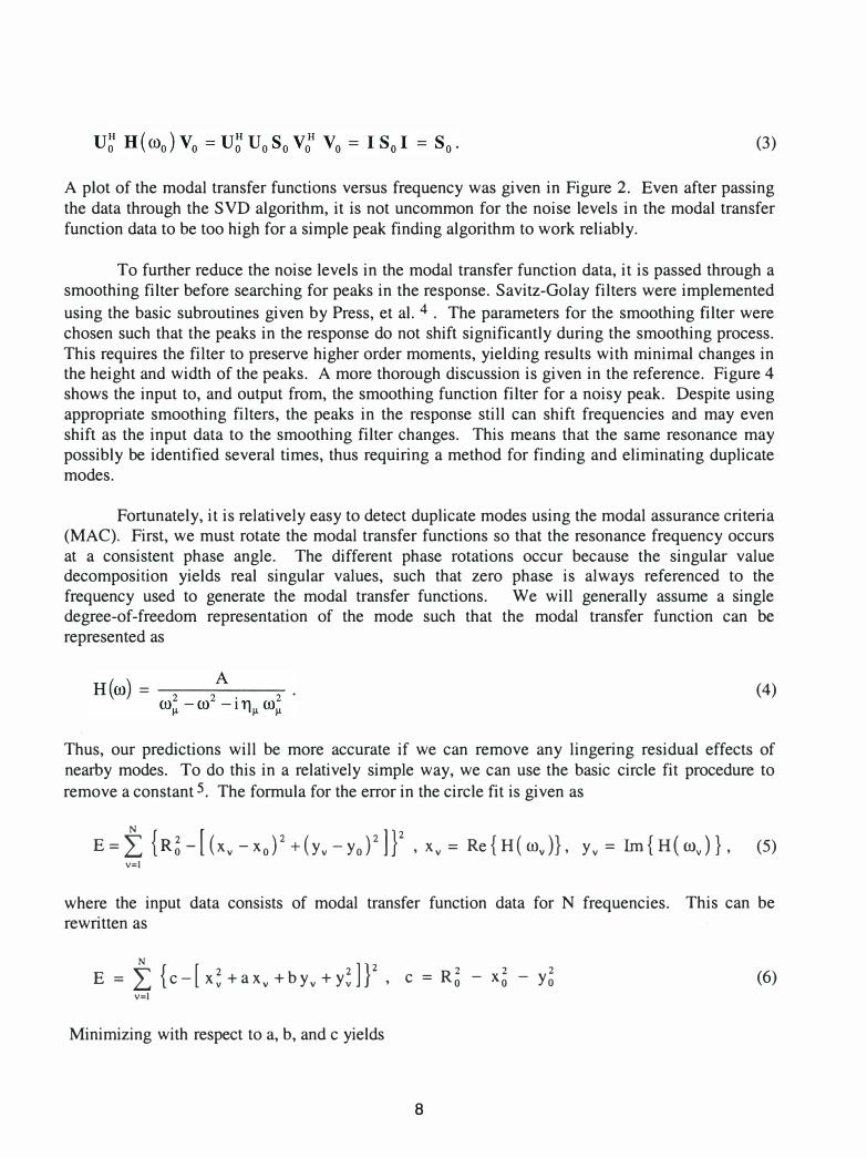
(3) A plot of the modal transfer functions versus frequency was given in Figure 2. Even after passing the data through the SVD algorithm, it is not uncommon for the noise levels in the modal transfer function data to be too high for a simple peak finding algorithm to work reliably.

To further reduce the noise levels in the modal transfer function data, it is passed through a smoothing filter before searching for peaks in the response. Savitz-Golay filters were implemented using the basic subroutines given by Press, et al. 4 . The parameters for the smoothing filter were chosen such that the peaks in the response do not shift significantly during the smoothing process. This requires the filter to preserve higher order moments, yielding results with minimal changes in the height and width of the peaks. A more thorough discussion is given in the reference. Figure 4 shows the input to, and output from, the smoothing function filter for a noisy peak. Despite using appropriate smoothing filters, the peaks in the response still can shift frequencies and may even shift as the input data to the smoothing filter changes. This means that the same resonance may possibly be identified several times, thus requiring a method for finding and eliminating duplicate modes.

Fortunately, it is relatively easy to detect duplicate modes using the modal assurance criteria (MAC). First, we must rotate the modal transfer functions so that the resonance frequency occurs at a consistent phase angle. The different phase rotations occur because the singular value decomposition yields real singular values, such that zero phase is always referenced to the frequency used to generate the modal transfer functions. We will generally assume a single degree-of-freedom representation of the mode such that the modal transfer function can be represented as

(4) Thus, our predictions will be more accurate if we can remove any lingering residual effects of nearby modes. To do this in a relatively simple way, we can use the basic circle fit procedure to remove a constant 5. The formula for the error in the circle fit is given as

E= I {R�- [ (xv- x0)2+ (yv- y0)2]Y , xv= Re{H (wJ}, Yv= Im{H(wJ}, (5) V=l

where the input data consists of modal transfer function data for N frequencies. This can be rewritten as

N

E = L { c - [ x� +a xv +byv +y� ] Y , c = R� - X� - y� (6) V=l

Minimizing with respect to a, b, and c yields

8

N N N N I x� I xv Yv -Ixv

m= -I(x�+xvy� )

V=l V=l V=l V=l N N N N

Ixv Yv I Y� - I Yv - I (y� + Yv X � ) (7) V=l V=l V=( V=l

N N N

- I xv - I Yv N I (x� +y� ) V=l V=l V=l

In the actual calculations, a weighting function is applied before solving the equation so that the data points near the resonance peak are more heavily weighted. This helps to reduce the residual effects of nearby modes in the circle fit algorithm. After solving for a, b, and c, the circle's center and its radius can be calculated as

(8)

If the modal circle's radius R0 is considerably smaller than the radial distance from the origin to its center Reenter , then the residual contribution from nearby modes is larger than that of the mode itself and the data likely represents an extraneous peak. Although there is no hard rule for when to filter out modes, we haye chosen to keep modes only when Reenter < 3 R0 , which provides a good balance between filtering out extraneous peaks and mistakenly filtering out actual modes. With the results from the circle fit algorithm, we can remove a constant representing the residual effects of nearby modes as

H ( wJ = H ( wJ - (a I 2 + i b I 2). (9) We can also rotate the modal circle so that the resonance frequency is aligned with the positive y­axis and translate it by the radius in the y-direction so that it passes through the origin. The result is

( 10)

where ao is the reference phase angle for the resonance frequency, which can be computed using divided differences 5. Figure 5 shows Nyquist plots of modal transfer function data before and after the transformation is applied. Applying the same phase rotation to the associated left-singular vector gives it a consistent phase angle regardless of which U and V matrices are used to compute the modal transfer functions in Equation (2). Thus, when we compute the modal assurance criteria (MAC) to try to determine if any of the modes are duplicates, they all have the same phase reference. Using typical transfer function data, the resulting MAC values are consistently above 0.98 for duplicate modes.

Once we've determined that two modes are duplicates, we need a method of deciding which modal transfer function will yield better estimates for the modal parameters. Through trial and error, it was found that better predictions were obtained by retaining the modal transfer function

9

with the larger modal circle, as output from the least square fitting algorithm. In practice, there is little difference between the predictions if the resonance peaks are well resolved in frequency.

As we noted previously, the SVD algorithm reduces noise in the largest singular values at the expense of the lowest singular values, which is desirable because most of the relevant modal peaks occur in the few largest singular values. Thus, the lowest singular values have relatively high noise levels and do not contain relevant information. To avoid identifying numerous extraneous peaks in the lowest singular values, the user can choose to apply the peak finding algorithm to only a few of the largest singular values. The parameter NP in the text input file in. txt, an example of which is listed in the appendix, is used to specify the number of singular values to search for peaks. As a general rule, the lowest singular value should always be excluded from the search. If the code stops because the array VSQ_MODE is out of bounds, the number of singular values to search to find response peaks must be reduced.

B. Modal Parameter Identification

The last step in the process is to actually determine the resonance frequencies and loss factors from the modal data. There are many methods for computing the modal parameters once the data for a single mode has been isolated. We have developed a simple least squares method for determining the parameters. The basic idea is to assume the modal transfer function for mode J.! can be represented in the form

A (11)

where A and B are complex constants. Then we can write the reciprocal of the modal transfer function as

(12)

In this form, the constant can be determined using linear least squares, making the solution much more reliable and efficient than an iterative nonlinear least squares solution. The error in the least square fit is calculated as

(13)

Taking the derivative with respect to the constants gives

10

(14)

Setting the derivatives equal to zero and rewriting the equations to solve for the constants gives the normal equations as

N N I w�

V=J N N I w� I m�

V=J V=J

{ ::} =

N L [ 1/ Hl1 ( wJ ] V=J N L [ w� / Hl1 ( wJ J

V=l

Solving for the constants yields the resonance frequency loss factor as

(15)

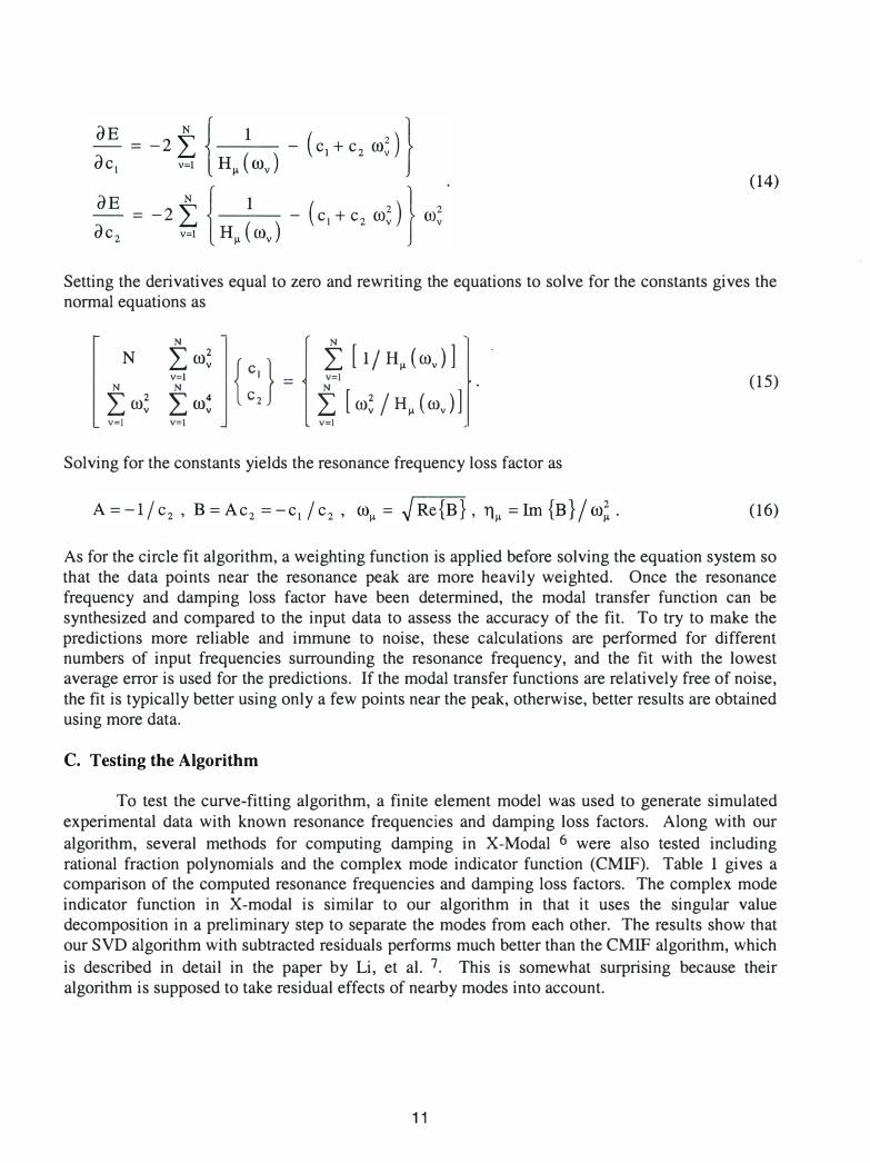
(16) As for the circle fit algorithm, a weighting function is applied before solving the equation system so that the data points near the resonance peak are more heavily weighted. Once the resonance frequency and damping loss factor have been determined, the modal transfer function can be synthesized and compared to the input data to assess the accuracy of the fit. To try to make the predictions more reliable and immune to noise, these calculations are performed for different numbers of input frequencies surrounding the resonance frequency, and the fit with the lowest average error is used for the predictions. If the modal transfer functions are relatively free of noise, the fit is typically better using only a few points near the peak, otherwise, better results are obtained using more data.

C. Testing the Algorithm

To test the curve-fitting algorithm, a finite element model was used to generate simulated experimental data with known resonance frequencies and damping loss factors. Along with our algorithm, several methods for computing damping in X-Modal 6 were also tested including rational fraction polynomials and the complex mode indicator function (CMIF). Table 1 gives a comparison of the computed resonance frequencies and damping loss factors. The complex mode indicator function in X-modal is similar to our algorithm in that it uses the singular value decomposition in a preliminary step to separate the modes from each other. The results show that our SVD algorithm with subtracted residuals performs much better than the CMIF algorithm, which is described in detail in the paper by Li, et al. 7. This is somewhat surprising because their algorithm is supposed to take residual effects of nearby modes into account.

1 1

D. Step-By-Step Analysis Procedure

The following steps will yield predictions for the resonance frequencies and damping loss factors from a set of transfer function data. The optional steps should be performed if mode shapes are to be computed as well.

( 1) Convert the experimental transfer function data to uff (universal file format) for dataset 58. An excerpt from a sample uff file is given in the appendix. If the data is in vna file format, the MA TLAB program UFF (included in the Siglab folder) can be used to perform the conversion. The resulting file should be named exp_data.txt.

(2) (Optional) Generate a geometry file representing the surface locations where the transfer function data was taken. It should be in the standard format for input files to the boundary element program POWER and should be named geom. txt. An excerpt from a sa:nple geom. txt file is given in the appendix.

(3) (Optional) Generate an in. txt file, which contains input values for the parameters. An excerpt from a sample in. txt file is given in the appendix.

(4) Run the program CONV_EXPERIMENTAL to automatically identify the resonance frequencies, damping loss factors, and (possibly) mode shapes. As mentioned in the text, a number of extraneous modes are inevitably identified.

NOTE: If the program crashes because it finds too many modes, the parameter NP in the in. txt file should be reduced such that fewer singular values are searched for peaks during the automatic identification process.

(5) Run the MATLAB function siftSVD to edit out the extraneous peaks.

In step (5), the user must pick which modes to keep and which modes to edit out. To help make the process easier, each modal transfer function is plotted, one at a time, overlaid on a plot of the singular values. Also, a secondary plot shows the phase for the modal transfer function. The user is then prompted to choose, yes or no, if the mode should be retained. As a general guideline, if the red line in the figure marking the resonance frequency does not line up with a peak in the modal transfer function, then the data likely represents an extrane us peak. Similarly, if the phase does not go through a 180 shift through the resonance, it should also be omitted. While this technique works very well for modes with low damping, it can be somewhat subjective for highly damped modes, where the actual resonance frequency does not necessarily line up with the peak in the response.

E. Future Work

Although the program works very well as it is, there two main areas in which it could be improved. First, the automatic procedures for eliminating extraneous modes could be refined so that the subsequent manual elimination process would be less time-consuming and tedious. Second, a more sophisticated algorithm could be implemented to help reduce or eliminate residual

12

effects in the identification of the resonance frequencies and loss factors. For example, rational fraction polynomials might be used in place of the simple least square fitting algorithm.

REFERENCES

1 D. Formenti and M. Richardson, "Parameter estimation from frequency response measurements using rational fraction polynomials (twenty years of progress)," in Proceedings of the

Twentieth International Modal Analysis Conference, pp. 373-382, 2002.

2 C. Y. Shih, Y. G. Tsuei, R. J. Allemang, and D. L. Brown, "Complex mode indication function and its applications to spacial domain parameter estimation," in Proceedings of the Seventh International Modal Analysis Conference, pp. 533-540, 1989.

3 A. W. Phillips, R. J. Allemang, and W. A. Fladung, "The complex mode indication function (CMIF) as a parameter estimation method," in Proceedings of the Sixteenth International Modal Analysis Conference, pp. 705-7 10, 1998.

4 W. H. Press, S. A. Teukolsky, W. T. Vetterling, and B. P. Flannery, Numerical Recipes in FORTRAN, (Cambridge University Press, Cambridge, 1992), pp. 644-649.

5 J. M. Montalvao, E Silva and N. M. M. Maia, "Single mode identification techniques for use with small microcomputers," in J. Sound. Vib., pp. 13-26, 1988.

6 From the University of Cincinnati Structural Dynamics Research Laboratory.

7 S. Li, W. A. Fladung, W. A. Phillips, and D. L. Brown, "Automotive applications of the enhanced mode indicator function parameter estimation method," in Proceedings of the Sixteenth International Modal Analysis Conference, pp. 36-44, 1998.

13

Table 1. Comparison of various methods for computing resonance frequencies and damping loss factors

Mode# 1 2 3 4 5 6 7 8 9 10 11 12

Exact Frequency 10.0 16.9 26.0 50.8 130.6 226.0 238.4 272.3 373.6 412.6 417.4 431.2

SVD with subtracted 9.9 17.1 25.9 50.9 130.7 226.0 272.2 373.5 412.8 417.4 431.2 residuals

SVD without 10.0 17.0 26.2 50.9 130.6 226.0 238.4 272.3 373.6 412.6 417.6 431.2 subtracted residuals I

X-Modal Rational 10.0 16.8 26.7 130.8 226.0 238.4 272.9 373.6 412.5 417.4 431.2 Fraction Polynomial I

....... X-Modal Complex 10.0 15.3 26.3 51.0 130.6 226.0 238.4 272.3 373.5 412.6 431.3 � Mode Indicator Func.

Exact Loss Factor 0.1 0.1 0.1 0.016 0.006 0.004 0.002 0.002 0.008 0.001 0.004 0.002

SVD with subtracted 0.099 0.107 0.097 0.017 0.006 0.004 0.002 0.008 0.001 0.004 0.002 residuals

SVD without 0.104 0.119 0.135 0.017 0.006 0.004 0.002 0.002 0.008 0.001 0.006 0.002 subtracted residuals

X-Modal Rational 0.095 0.106 0.254 0.006 0.004 0.001 0.002 0.008 0.001 0.004 0.002 Fraction Polynomial

X-Modal Complex 0.083 0.063 0.051 0.014 0.006 0.004 0.002 0.002 0.008 0.001 0.002 Mode Indicator Func.

co "0 en Q) ::J ctS

> '-...... ctS (J1 ::J 0) -�

(f)

-1 0�----�----�----�----�----�----�----�----�

-20

-30

_......../

!-- ....................

I. rr r I / \ v/''\ I / \ I \1 /\ ;7 ---\�r-7 \

J II 'I / \ / - \ / " r / ,-' ',,_ "\. '-...../ - - - -- ._ .......... ..........

/ . ' ',______ ,-- '. "

- · - . -

· 1-.-

- ' ' '

''"'"1·-·-._

...... " -----

... _ _ __

___ _ _

-. :_-: :..-: :. -:- :�.::..-.-.-.-.-.-.- � . .. . ...... . ... ... . ......... . ...... ... . f=---�:- .�:: · f··�-:f��::1- ·�::���1· .·��·-:-· =-�-t.;:;;:::.-:�r�-�.�:.��n��-��---�.�1� ··�.:..�-:.� �=:�� - _:-:--_ :-:-_-::-= ::-:: - - - - - - - , - - - - - - - - , - - - - - - - ' - - - - - - - - - - , , - - - - - - - - - - - - - - - - - - � · �- - - :':"--:-:. - =-=--�-:::--=- .:-::-_-::-

�·- . - . . - · -· - . - . - . � .� : �.·.� : �.· .� ·.-:- .- � ·.-:- : �:.-: : -:-:.-: : � ·.-:- : :-: ·.- :- : :-. · .--: : .. ·.-:- : � ·::· : :-. ·.-: : . · :-. ·.7 : :-. · . -: : :-. · . . : :-.·.-:·.-:- : :-. ·.-:- : :-. -40 I ...... .

��__,....�

-50�----�----�----�----�----�----�----�----�

40 50 60 Frequency, Hz

70

Figure 1. Singular values as a function of frequency for a series of closely-spaced modes

80

0 T"""

I

...

I

1/ < N I ./

� I"""

� � "'

/\11

v .: < I , , � ,'' � v ' '

( "'

"' \

\

0 C\J I

I I I

I I I I

I I I

I I I I

I ,/ I I

I I

I I ,

I

/ I I .\

\ \ ·

, I I I

I I I I I I

I I

I I

I I \ I

\ ·,

' ' \

\ \

\ \

\ \

\ I

\ \ \ \ \

I

\

I I I ' I

I I

I

I I

I I I

I : I

·� . ·: \

·. \ ': 1

I

I I I I

I I I

I I I I I I• II I' II I' II !t :

0 Cl') I

16

� )

��� � 1: I

) I ill I 'I

I : l: )I I: 'I . I . ) I � �� I· 'I : : I: / 1 I �� ,: � I : I .

. \;!\ , I: . '( r I. :_t I I i: ; :d �: I: :'Iii' ..

. I . I I'

: 1!1� 1 I: I � : : , ;� I

. Ill I I: '�;I I ( . '

,: � I I: I I :'I I .. I \ : 1 il I

\: I I

I :� I > . I : • I I I I·.

:, I I � : I . -·: r 11 ? II i: } 1 I .11 : . I ( : I

: \ l �� I : •. I I i l I ,

: I:. ' : n I

': \I ( I J I ·: \ �� .: I I ) ' �.� I ? : :P.: I

��� I

. I )� l I I :,,,I I I : ''! \ I

. \ I: I I : ( q I . ) l : .

i 1 ! t>_ : : ) J -1 ' iII h : ;·I 1 t) � : I .. , ; I i \ :

l: j_ :_i:

I I I I \

I I I I I I I I I I I

� I_ I ) i I

0 -.:::t I

\ J )

} 1 �

�

0 co

0 ,........

0 c.o

0 l.()

0 0-.:::t l.() I

>. (.) c Q) :J 0"' Q) .... --0 c 0

·.;= (.) c :J -co C/) co C/) Q) :J co > .... co

N :J C) I c

·u; >. Q) () ..c c: -Q) c :::J 0 0"' "0 Q) ·ca lo... "C u. Q) > 0

C/) c 0 :;::: (.) c :J -.... Q) -C/) c co .... -co "0 0 � C\1 Q) .... :J C) u::

0.006

0.004

0.002

.......

-....j 0.000

. �v �� ...;V' \ \ 1\

.....-. � I I I I I .....-. N N

0.003

0.002

0.001

- -0.002 7

� I ,

- 0.000

E -0.004

-0.006

-0.008

-0.010

\ ; ju. " v

'� // I "" .t.

0.000 0.002 0.004 0.006 0.008 0.010 0.012 0.014 0.016

Re { Z}

E

-0.001

-0.002

-0.003 0.000 0.001 0.002 0.003

Re { Z}

Figure 3. Circle fits for two overlapping modes using modal transfer functions

0.004 0.005 0.006

co "0 CJ) Q) ::::s ro

> '-....... ro

CXl ::::s 0> .� (f)

-30

-31

-32

-33

-34

-35 3030

-

if\� � � � -J .......... • .... v< t A a· �

If/ I'

J/ J

� fl

3040 3050 3060 Frequency, Hz

3070

�

• Input Output

� � \ \ \ � -�

3080

Figure 4. Input to, and output from, the Savitz-Golay smoothing filter

1----

I

3090

0.015

... "' / 0.010

_.. 0.005 <0

-N - 0.000

E --0.005

... 1\.. .......

"' � -0.010

-0.015 -0.005 0.000 0.005

v

�

... ...

0.010

Re { Z}

r--......

-� 0.015

' )!. �

\

j v

0.020

0.025

0.020

0.015

�. \ -N - 0.010

E

1 j 0.005

0.000

-0.005 0.025 -0.015 -0.010 -0.005 0.000 0.005

Re { Z}

Figure 5. Original circle fit and circle fit after subtracting residual terms and rotating

0.010 0.015

APPENDIX

Excerpt from a sample exp data. txt file:

-1 58

22-Nov-02 15:19:04

NONE Data Source: DSPt vna_2 file

22-Nov-02 15:19:04 Channel 1 Channel 2 NONE

4 0 0 0 NONE 43 3 NONE 1 5

18 12 13

3201 1 O.OOOOOE+OO 1.56250E-01 O.OOOOOE+OO

0 1. 73138E-02 3.87860E-03 1.25638E-03

0 0 0 0 0 0 0 0 0 0 0 0

O.OOOOOE+OO -2 .13539E-03 -1.35666E-03

7.08637E-02 -9.17354E-03 7.45084E-02 -4.43652E-03 6.46172E-02 -1.51906E-02

-1 -1 58

NONE NONE NONE NONE NONE NONE NONE NONE

7.91415E-03 -1.53991E-02 2. 71964E-04 -9.14080E-04 1.39712E-03 -2.15564E-03

6. 75563E-02 -7.72947E-03 8.05078E-02 -1.49483E-03 6.05182E-02 1.79914E-03

-6.67674E-03 -1.06145E-02 2.18173E-03 -9.62644E-04 1.37733E-03 -1.26802E-03

6.81926E-02 -1.32550E-03 7.32544E-02 -2.39376E-03 6.63789E-02 4.58963E-03

22-Nov-02 15:19:04 NONE

Data Source: DSPt vna_2 file

22-Nov-02 15:19:04 Channel 1 Channel 3 NONE

4 0 0 0 NONE 48 3 NONE 1 5 3201 1 O.OOOOOE+OO 1.56250E-01 O.OOOOOE+OO

18 12 13

0 4.48223E-03 8.73688E-04 7.07169E-04

0 0 0 0 0 0 0 0 0 0 0 0

O.OOOOOE+OO -1.31413E-03

1.16311E-04

NONE NONE NONE NONE

7.08740E-04 4.80697E-05

-6.57040E-04

Excerpt from a sample geom. txt file:

GRID GRID GRID

GRID GRID GRID

$ CQUAD4 CQUAD4 CQUAD4 CTRIA3

1 2 3

128 129 130

1 2 3 4

0 0.0938 1.59375 0 0.0938 3.59375 0 0.0938 5.59375

0 24.0938 14.5938 0 24.0938 16. 5938 0 24.0938 18.5938

0 1 11 0 3 2 0 4 3 0 6 8

NONE NONE NONE NONE

-4.42584E-03 4.87825E-04

-9.21849E-04

12. 12. 12.

12. 12. 12.

12 12 13 10

20

-2.97309E-03 1.28667E-03 8.07705E-04

0

0 0

0 0 0

2 13 14

2. 2. 2. 2.

1.38174E-02 -2.22795E-03

4.08600E-04

3

3

CTRIA3

CQUAD4 CQUAD4 CQUAD4 $END

5

106 107 108

0

0 0 0

9

117 118 119

15

127 128 129

17

128 129 130

118 119 120

2.

2. 2. 2.

Excerpt from a sample in. txt file:

$ $ $ $ $

CF ss CI IB pp uv AG IO GF $ $ $

GN ND NP RS

INPUT DEFAULT

DATA USED BY ALL PROGRAMS (Defaults in parentheses)

0.0254 1500.0 1.5E6 1 3 1.0 0.0 018 -1 18

(1. 0) (343.0) (415.0) (1) (0)

0.0 (1) ( -1) (1)

Input conv. factor for nodal loc. & disp. Input the sound speed Input the characteristic impedance Input 0 for infinite baffle (z=O plane) Input 0, 1, 2, 3 for no ouput, Hypermesh, FEMAP mfr, or FEMAP modes Input the unit vector for the axis of rotational symmetry Input the number of angular sections Input the desired circumferential component Input the number of angular sections for part 1

DATA USED BY CONV_EXPERIMENTAL, CONV_NASTRAN

1.0 1 0 1

(1.0) (1) (0) (1)

Input a gain (and/or sensitivity) for the exp. data Input the drive point number for the integrated squared velocity Input the number of singular values to search for peaks ( 0 = NM-1 Input 1 to subtract residuals from the circle fits

2 1