NAVIGATION ALGORITHM FOR SPACECRAFT

LUNAR LANDING

By

Sasikanth Venkata Sai Paturi

A ThesisSubmitted to the Faculty ofMississippi State University

in Partial Fulfillment of the Requirementsfor the Degree of Master of Science

in Aerospace Engineeringin the Department of Aerospace Engineering

Mississippi State, Mississippi

August 2010

UMI Number: 1479262

All rights reserved

INFORMATION TO ALL USERS The quality of this reproduction is dependent upon the quality of the copy submitted.

In the unlikely event that the author did not send a complete manuscript

and there are missing pages, these will be noted. Also, if material had to be removed, a note will indicate the deletion.

UMI 1479262

Copyright 2010 by ProQuest LLC. All rights reserved. This edition of the work is protected against

unauthorized copying under Title 17, United States Code.

ProQuest LLC 789 East Eisenhower Parkway

P.O. Box 1346 Ann Arbor, MI 48106-1346

NAVIGATION ALGORITHM FOR SPACECRAFT

LUNAR LANDING

By

Sasikanth Venkata Sai Paturi

Approved:

Yang ChengAssistant Professor ofAerospace Engineering(Major Professor)

Ming XinAssistant Professor ofAerospace Engineering(Committee Member)

Pasquale CinnellaProfessor and Head ofAerospace Engineering(Committee Member)

Mark JanusGraduate Coordinator andAssociate Professor ofAerospace Engineering

Sarah A. RajalaDean of the James Worth BagleyCollege of Engineering

Name: Sasikanth Venkata Sai Paturi

Date of Degree: August 7, 2010

Institution: Mississippi State University

Major Field: Aerospace Engineering

Major Professor: Dr. Yang Cheng

Title of Study: NAVIGATION ALGORITHM FOR SPACECRAFT LUNAR LAND-ING

Pages in Study: 114

Candidate for Degree of Master of Science

A detailed analysis and design of a navigation algorithm for a spacecraft to achieve

precision lunar descent and landing is presented. The Inertial Navigation System (INS)

was employed as the primary navigation system. To increase the accuracy and precision

of the navigation system, the INS was integrated with aiding sensors - a star camera, an

altimeter and a terrain camera. An unscented Kalman filter was developed to integrate the

aiding sensor measurements with the INS measurements, and to estimate the current posi-

tion, velocity and attitude of the spacecraft. The errors associated with the accelerometer

and gyro measurements are also estimated as part of the navigation filter. An STK sce-

nario was utilized to simulate the truth data for the navigation system. The navigation filter

developed was tested and simulated, and from the results obtained, the position, velocity

and attitude of the spacecraft were observed to be well estimated.

ACKNOWLEDGMENTS

I offer my sincerest gratitude to my advisor, Dr. Yang Cheng, who has guided and

supported me with his never ending patience and knowledge whilst allowing me the room

to work in my own way. He has been a great mentor and friend. I am grateful to my

committee members, Dr. Cinnella and Dr. Xin, for understanding my needs and helping

me in every possible way during the last two years.

A very special expression of appreciation is due to Mr. Mike Loucks of Space Explo-

ration Engineering (SEE) Corporation, for his selfless assistance in providing me with the

required STK scenarios.

I would like to thank the students, faculty and staff of the Aerospace Engineering

department for having created an enjoyable and productive work environment. A special

thanks to my officemate, Brett Zeigler, with whom I have shared incredibly diverse and

pondering conversations.

I wish to thank my parents for their unconditional love and support, my brother Sivakanth,

for always believing in me, and my friend Soumya Nair, for everything.

Last, but hardly least, I would like to thank the Almighty, for being the light through

many a dark hour.

ii

TABLE OF CONTENTS

ACKNOWLEDGMENTS . . . . . . . . . . . . . . . . . . . . . . . . . . . . . . . ii

LIST OF TABLES . . . . . . . . . . . . . . . . . . . . . . . . . . . . . . . . . . v

LIST OF FIGURES . . . . . . . . . . . . . . . . . . . . . . . . . . . . . . . . . . vi

CHAPTER

1. INTRODUCTION . . . . . . . . . . . . . . . . . . . . . . . . . . . . . . 1

1.1 Motivation . . . . . . . . . . . . . . . . . . . . . . . . . . . . . . . 11.2 Thesis Overview . . . . . . . . . . . . . . . . . . . . . . . . . . . . 41.3 Organization of Thesis . . . . . . . . . . . . . . . . . . . . . . . . . 5

2. INERTIAL NAVIGATION SYSTEM AND AIDING SENSORS . . . . . . 7

2.1 Navigation System Overview . . . . . . . . . . . . . . . . . . . . . 72.1.1 Coordinate Frames . . . . . . . . . . . . . . . . . . . . . . . 82.1.2 Sensors . . . . . . . . . . . . . . . . . . . . . . . . . . . . . 82.1.3 Mechanization Equations . . . . . . . . . . . . . . . . . . . . 92.1.4 Navigation Errors . . . . . . . . . . . . . . . . . . . . . . . . 9

2.2 Inertial Navigation System . . . . . . . . . . . . . . . . . . . . . . . 92.2.1 Classification of INS . . . . . . . . . . . . . . . . . . . . . . 122.2.2 INS equations . . . . . . . . . . . . . . . . . . . . . . . . . . 16

2.3 Dynamic Models . . . . . . . . . . . . . . . . . . . . . . . . . . . . 172.3.1 Gravity . . . . . . . . . . . . . . . . . . . . . . . . . . . . . 172.3.2 Attitude Quaternion Kinematics . . . . . . . . . . . . . . . . 20

2.4 IMU Sensor Models . . . . . . . . . . . . . . . . . . . . . . . . . . 222.4.1 Accelerometers . . . . . . . . . . . . . . . . . . . . . . . . . 222.4.2 Gyroscopes . . . . . . . . . . . . . . . . . . . . . . . . . . . 25

2.5 Aiding Sensor Models . . . . . . . . . . . . . . . . . . . . . . . . . 272.5.1 Altimeter . . . . . . . . . . . . . . . . . . . . . . . . . . . . 292.5.2 Terrain Camera . . . . . . . . . . . . . . . . . . . . . . . . . 302.5.3 Star Camera . . . . . . . . . . . . . . . . . . . . . . . . . . 32

iii

3. KALMAN FILTERING . . . . . . . . . . . . . . . . . . . . . . . . . . . 34

3.1 Kalman Filter . . . . . . . . . . . . . . . . . . . . . . . . . . . . . . 343.1.1 Covariance . . . . . . . . . . . . . . . . . . . . . . . . . . . 353.1.2 Continuous-Discrete Kalman Filter . . . . . . . . . . . . . . 36

3.2 Extended Kalman Filter . . . . . . . . . . . . . . . . . . . . . . . . 383.2.1 Continuous-Discrete Extended Kalman Filter . . . . . . . . . 39

3.3 Unscented Kalman Filter . . . . . . . . . . . . . . . . . . . . . . . . 403.3.1 Unscented Transformation . . . . . . . . . . . . . . . . . . . 433.3.2 Unscented Kalman Filter . . . . . . . . . . . . . . . . . . . . 45

3.4 Application of Kalman Filter to Aided INS . . . . . . . . . . . . . . 48

4. NAVIGATION SYSTEM AND ALGORITHM . . . . . . . . . . . . . . . 49

4.1 Landing Scenario . . . . . . . . . . . . . . . . . . . . . . . . . . . . 494.2 Navigation System Block Diagram . . . . . . . . . . . . . . . . . . 504.3 Unscented Kalman Filter for Navigation System . . . . . . . . . . . 52

4.3.1 Navigation System and Measurement Dynamics . . . . . . . 544.3.2 Sigma Points . . . . . . . . . . . . . . . . . . . . . . . . . . 564.3.3 Propagation and Update without Measurements . . . . . . . . 574.3.4 Propagation and Update with Measurements . . . . . . . . . 59

5. NAVIGATION SYSTEM PERFORMANCE ANALYSIS . . . . . . . . . 63

5.1 Mission Scenario . . . . . . . . . . . . . . . . . . . . . . . . . . . . 635.2 STK Scenario . . . . . . . . . . . . . . . . . . . . . . . . . . . . . . 675.3 Estimation Error Results . . . . . . . . . . . . . . . . . . . . . . . . 72

5.3.1 Inertial Navigation System . . . . . . . . . . . . . . . . . . . 725.3.2 INS and Star Camera . . . . . . . . . . . . . . . . . . . . . . 765.3.3 INS and Altimeter . . . . . . . . . . . . . . . . . . . . . . . 765.3.4 INS and Terrain Camera . . . . . . . . . . . . . . . . . . . . 835.3.5 INS, Star Camera and Altimeter . . . . . . . . . . . . . . . . 875.3.6 INS, Star Camera and Terrain Camera . . . . . . . . . . . . . 875.3.7 INS, Altimeter and Terrain Camera . . . . . . . . . . . . . . 945.3.8 INS, Star Camera, Altimeter and Terrain Camera

(Integrated Navigation System) . . . . . . . . . . . . . . . . 985.4 Monte Carlo Simulation Results . . . . . . . . . . . . . . . . . . . . 104

6. CONCLUSIONS . . . . . . . . . . . . . . . . . . . . . . . . . . . . . . . 109

REFERENCES . . . . . . . . . . . . . . . . . . . . . . . . . . . . . . . . . . . . . 111

iv

LIST OF TABLES

2.1 Lunar Constants . . . . . . . . . . . . . . . . . . . . . . . . . . . . . . . . . 18

2.2 Zonal Harmonic Parameters . . . . . . . . . . . . . . . . . . . . . . . . . . . 19

5.1 Random Error Standard Deviation Values . . . . . . . . . . . . . . . . . . . 65

5.2 Random Noise Standard Deviation Values . . . . . . . . . . . . . . . . . . . 65

5.3 Unscented Transformation Parameters . . . . . . . . . . . . . . . . . . . . . 67

v

LIST OF FIGURES

2.1 Inertial Navigation System . . . . . . . . . . . . . . . . . . . . . . . . . . . 11

2.2 Inertial Sensor Assembly . . . . . . . . . . . . . . . . . . . . . . . . . . . . 13

2.3 Gimbaled IMU . . . . . . . . . . . . . . . . . . . . . . . . . . . . . . . . . 14

2.4 Floated IMU . . . . . . . . . . . . . . . . . . . . . . . . . . . . . . . . . . . 15

2.5 Strapdown ISA . . . . . . . . . . . . . . . . . . . . . . . . . . . . . . . . . 15

2.6 Schematic Diagram of an Accelerometer . . . . . . . . . . . . . . . . . . . . 23

2.7 Schematic Diagram of a Gyroscope . . . . . . . . . . . . . . . . . . . . . . 26

2.8 Basic principle of Aided INS . . . . . . . . . . . . . . . . . . . . . . . . . . 28

3.1 Sigma points for a 2-dimensional Gaussian Random Variable . . . . . . . . . 41

3.2 Unscented Transformation . . . . . . . . . . . . . . . . . . . . . . . . . . . 44

3.3 Comparison between EKF and UKF . . . . . . . . . . . . . . . . . . . . . . 47

4.1 Descent-to-Landing Scenario . . . . . . . . . . . . . . . . . . . . . . . . . . 50

4.2 Navigation System . . . . . . . . . . . . . . . . . . . . . . . . . . . . . . . 51

5.1 Ground Track of the Landing Trajectory . . . . . . . . . . . . . . . . . . . . 63

5.2 Altitude Profile of the Landing Trajectory . . . . . . . . . . . . . . . . . . . 64

5.3 Location of Lunar Feature Points . . . . . . . . . . . . . . . . . . . . . . . . 65

5.4 Measurement Times of the Aiding Sensors . . . . . . . . . . . . . . . . . . . 66

5.5 Screen Captures of the Spacecraft Descent-to-Landing . . . . . . . . . . . . 68

vi

5.6 Position Data obtained from STK Scenario . . . . . . . . . . . . . . . . . . . 69

5.7 Velocity Data obtained from STK Scenario . . . . . . . . . . . . . . . . . . . 70

5.8 Quaternion Data obtained from STK Scenario . . . . . . . . . . . . . . . . . 70

5.9 Acceleration Data obtained from STK Scenario . . . . . . . . . . . . . . . . 71

5.10 Angular Velocity Data obtained from STK Scenario . . . . . . . . . . . . . . 71

5.11 INS - Position Estimation Error . . . . . . . . . . . . . . . . . . . . . . . . . 73

5.12 INS - Velocity Estimation Error . . . . . . . . . . . . . . . . . . . . . . . . . 74

5.13 INS - Quaternion Estimation Error . . . . . . . . . . . . . . . . . . . . . . . 75

5.14 INS & Star Camera - Position Estimation Error . . . . . . . . . . . . . . . . 77

5.15 INS & Star Camera - Velocity Estimation Error . . . . . . . . . . . . . . . . 78

5.16 INS & Star Camera - Quaternion Estimation Error . . . . . . . . . . . . . . . 79

5.17 INS & Altimeter - Position Estimation Error . . . . . . . . . . . . . . . . . . 80

5.18 INS & Altimeter - Velocity Estimation Error . . . . . . . . . . . . . . . . . . 81

5.19 INS & Altimeter - Quaternion Estimation Error . . . . . . . . . . . . . . . . 82

5.20 INS & Terrain Camera - Position Estimation Error . . . . . . . . . . . . . . . 84

5.21 INS & Terrain Camera - Velocity Estimation Error . . . . . . . . . . . . . . . 85

5.22 INS & Terrain Camera - Quaternion Estimation Error . . . . . . . . . . . . . 86

5.23 INS, Star Camera & Altimeter - Position Estimation Error . . . . . . . . . . . 88

5.24 INS, Star Camera & Altimeter - Velocity Estimation Error . . . . . . . . . . 89

5.25 INS, Star Camera & Altimeter - Quaternion Estimation Error . . . . . . . . . 90

5.26 INS, Star Camera & Terrain Camera - Position Estimation Error . . . . . . . 91

5.27 INS, Star Camera & Terrain Camera - Velocity Estimation Error . . . . . . . 92

vii

5.28 INS, Star Camera & Terrain Camera - Quaternion Estimation Error . . . . . . 93

5.29 INS, Altimeter & Terrain Camera - Position Estimation Error . . . . . . . . . 95

5.30 INS, Altimeter & Terrain Camera - Velocity Estimation Error . . . . . . . . . 96

5.31 INS, Altimeter & Terrain Camera - Quaternion Estimation Error . . . . . . . 97

5.32 Integrated Navigation System - Position Estimation Error . . . . . . . . . . . 99

5.33 Integrated Navigation System - Velocity Estimation Error . . . . . . . . . . . 100

5.34 Integrated Navigation System - Quaternion Estimation Error . . . . . . . . . 101

5.35 Integrated Navigation System - Accelerometer Bias Estimation Error . . . . . 102

5.36 Integrated Navigation System - Gyroscope Bias Estimation Error . . . . . . . 102

5.37 Integrated Navigation System - Accelerometer Scale Factor Estimation Error 103

5.38 Integrated Navigation System - Gyroscope Scale Factor Estimation Error . . . 103

5.39 Monte Carlo Analysis - Position Estimation Error . . . . . . . . . . . . . . . 105

5.40 Monte Carlo Analysis - Velocity Estimation Error . . . . . . . . . . . . . . . 105

5.41 Monte Carlo Analysis - Quaternion Estimation Error . . . . . . . . . . . . . 106

5.42 Monte Carlo Analysis - Accelerometer Bias Estimation Error . . . . . . . . . 106

5.43 Monte Carlo Analysis - Gyroscope Bias Estimation Error . . . . . . . . . . . 107

5.44 Monte Carlo Analysis - Accelerometer Scale Factor Estimation Error . . . . . 107

5.45 Monte Carlo Analysis - Gyroscope Scale Factor Estimation Error . . . . . . . 108

viii

CHAPTER 1

INTRODUCTION

1.1 Motivation

Through the ages, the Moon, our closest celestial body, has aroused curiosity in our

mind much more than any other objects in the sky. This led to scientific study of the Moon,

driven by human desire and quest for knowledge. Exploration of the Moon got a boost

with the advent of the space age and the decades of sixties and seventies saw a myriad of

successful unmanned and manned missions to the Moon. The physical exploration of the

Moon began when Luna 2, a space probe launched by the Soviet Union, made an impact on

the surface of the Moon on September 14, 1959. It was followed by National Aeronautics

and Space Administration’s (NASA) Project Apollo, which for the first time, successfully

landed humans on the Moon on July 20, 1969.

Over the years, new questions about lunar evolution emerged, and new possibilities

of using the Moon as a platform for further exploration of the solar system and beyond

were formulated. Almost 51 years since its first exploration, the recent discovery of the

widespread presence of water molecules in lunar soil by NASA’s Moon Mineralogy Map-

per, or M3 instrument carried aboard the Indian Space Research Organization’s (ISRO)

Chandrayaan-1 spacecraft [1] has created a new renaissance and interest in lunar explo-

rations.

1

While the former Soviet Union, the United States, the European Space Agency (ESA),

Japan and India have successfully achieved lunar impact and/or landing till date, all the

major space faring nations of the world plan missions to further explore the Moon, and to

utilize the lunar surface as a potential base for space exploration. Achieving such goals

allows humans to take the next step towards further exploration of Mars and beyond.

In 1994, Clementine, a deep space program science experiment by the Ballistic Missile

Defense Organization and NASA, discovered the possible existence of ice on the Moon

[2]. This mission was followed by NASA’s Lunar Prospector in 1998, and a robotic space-

craft LCROSS (Lunar Crater Observation and Sensing Satellite) in 2009, to explore the

presence of water ice on the Moon. Over the years, NASA plans to explore Mars, near

Earth and deep space Asteroids. As a precursor to future missions, NASA’s Lunar Recon-

naissance Orbiter (LRO) is currently orbiting the Moon to identify safe landing sites, locate

potential resources on the Moon, characterize the radiation environment, and demonstrate

new technology [3].

In 2003, ESA launched a lunar probe SMART-1, using solar-electric propulsion and

carrying a battery of miniaturized instruments. After completing a comprehensive inven-

tory of the Moon, the mission ended through lunar impact in 2006 [4]. ESA plans to launch

a lunar lander mission, followed by manned lunar missions in the next decade. ESA also

plans to explore and navigate through deep space with intentions of landing on Asteroids

and on Mars [5].

The Japanese Aerospace Exploration Agency (JAXA) launched its first lunar probe

Hiten in 1990, followed by another lunar orbiter Selene (Selenological and Engineering

2

Explorer) in 2007, which intentionally crash landed on the Moon in 2009. JAXA plans to

put humanoid robots on the moon by 2015, with a goal of constructing a manned lunar base

by 2020 [6]. JAXA’s Hayabusa successfully landed on an Asteroid in 2005 and returned

to Earth in 2010 [7].

India’s first mission to the Moon, Chandrayaan-1, was launched in 2008. The Moon

Impact Probe (MIP) onboard Chandrayaan-1 intentionally crash landed on the Moon, be-

fore it discovered lunar water in 2009. ISRO expects to launch an indigenous lunar mis-

sion, Chandrayaan-2, by 2013, which would place a motorized rover on the surface of the

Moon to improve understanding of its origin and evolution [8], and plan to send a lunar

manned mission by 2020.

After a series of lunar expeditions in the 1970’s, Russia plan to re-launch the Luna

missions. By the year 2012, they plan to launch an unmanned lunar mission including an

orbiter with ground penetrating sensors, followed by an orbiter rover mission, and expect

to set up a lunar base by 2025 [9].

China launched its first lunar orbiter Chang’e 1 in 2007. They plan to launch another

lunar orbiter Chang’e 2 in 2010, followed by a lunar probe Chang’e 3, intended to soft

land on the Moon in 2012, and a manned lunar mission by 2020 [10].

These missions, either to the Moon, Mars or deep space, currently face a number of

challenges, such as finding optimal solutions for low-energy and low-thrust orbit transfers,

formation flying, precise landing, autonomous navigation, autonomous landing, hazard

avoidance, rendezvous in deep space, etc. The current work addresses one such challenge

by developing a precision on-board navigation system for lunar landing. The landing phase

3

of the spacecraft plays an important role in the success of a lunar exploration mission and

a high-precision navigation algorithm is required to make a safe and successful landing

on the Moon. The aim of the thesis is to design such navigation algorithm, wherein the

inertial navigation system is integrated with aiding sensors such as an altimeter, terrain

camera and a star camera, to achieve precise lunar landing.

1.2 Thesis Overview

The role of navigation system is to provide an indication of the position and orientation

of the spacecraft with respect to a known reference frame. An inertial navigation system

(INS) is a navigation aid which uses motion sensors and rotation sensors to continuously

calculate the position, velocity and orientation of a moving spacecraft, and is one of the

most common navigation aids in aerospace applications. The INS systems are robust

systems and entirely self-contained within the vehicle, i.e., once initialized, they are not

dependent on any external resources [11]. This makes the INS applicable for deep space

landing missions wherein the gravitational model is accurately modeled, and is a major

advantage.

However, the INS systems rely upon the availability of accurate knowledge of the ini-

tial position of the spacecraft and its performance is characterized by time-dependent in-

tegration drift, wherein small errors in the measurements are integrated into progressively

larger errors in the current position. To overcome these disadvantages and to improve its

precision, the INS systems are integrated with certain aiding sensors. These systems are

known as integrated or aided navigation systems.

4

A Kalman filter is used to combine the inertial measurement data with the measure-

ments of the aiding sensors. Kalman filtering has become a well established technique

for the mixing of navigation data in integration systems [12]. The extended Kalman filter

has long been the workhorse of space-based navigation systems, dating back to the early

days of the Apollo missions. A more efficient method of Kalman filtering, the unscented

Kalman filter, is used to integrate the measurements in the current work.

Though the work presented is for a lunar landing mission, enabling certain additional

strategies makes the system applicable for deep space landing missions. An aided INS

controlled along a precise entry, descent and landing (EDL) trajectory, utilizing closed-

loop guidance methods can be applicable for Mars landing missions [13][14]. An insight

of a Mars entry navigation system using INS is presented in [15].

For the landing problem, it is important to optimally control and design the landing

trajectory in order to minimize the fuel consumption of the spacecraft. An optimal thrust

program for a lunar soft landing problem, based on an application of Pontryagin’s mini-

mum principle, was developed by Meditch in 1964 [16]. Over the years, with the increase

in computing power, various trajectory optimization techniques have been developed. A

few optimization techniques can be studied in [17], [18], [19], [20], [21].

1.3 Organization of Thesis

The organization of this work is as follows: Chapter 2 gives a brief overview of

navigation systems followed by the underlying concepts of the inertial navigation system,

working principle and modeling of the inertial measurement unit (IMU) sensors and the

5

aiding sensors. Chapter 3 describes the concept of Kalman filtering. The working of a

Kalman filter and an extended Kalman filter (EKF) for a continuous-discrete time system,

theory and working of an unscented Kalman filter (UKF), its advantages over the EKF,

and a brief on the application of the Kalman filtering technique to the integrated inertial

navigation system are discussed in this chapter.

Chapter 4 describes the working equations of the navigation algorithm in detail. De-

tails on the landing trajectory, landing scenario and the block diagram of the system being

considered are presented, followed by the filter structure, system dynamics and the fil-

tering algorithm. Chapter 5 discusses the simulation results obtained for the navigation

algorithm. The STK scenario used for the current work, and the inconsistencies in the data

obtained from the scenario are discussed. The simulated results obtained for the INS with-

out the aiding sensors, and for different combinations of the aiding sensors are presented.

The performance of the filter is studied from the results obtained and a discussion on the

aiding sensors which help achieve higher accuracy is presented. A summary of the results,

conclusions and a few recommendations for future work are presented in Chapter 6.

6

CHAPTER 2

INERTIAL NAVIGATION SYSTEM AND AIDING SENSORS

Navigation in simple terms is the process of finding the way from one place to an-

other. In systems and autonomous vehicle literature, navigation is to accurately determine

the position and velocity relative to a known reference, and if required, to maneuver the

vehicle between desired locations [11]. A few basic forms of space-based navigation are

discussed below [22].

• Pilotage: Relies on recognizing landmarks to know where and how the vehicle isoriented.

• Dead Reckoning: Relies on knowing where the vehicle started from, measurementsof speed and direction.

• Celestial Navigation: Uses time and the angles between local vertical and knowncelestial objects to estimate orientation, latitude, and longitude.

• Radio Navigation: Relies on radio frequency sources with known locations.

• Inertial Navigation: Relies on knowing the initial position, velocity, and attitude ofthe vehicle, and thereafter measuring the attitude rates and accelerations.

2.1 Navigation System Overview

A basic overview of the coordinate reference frames being considered in the current

work, the sensors and their errors is discussed in this section.

7

2.1.1 Coordinate Frames

The navigation process is defined relative to a known reference frame. The reference

here implies a specific coordinate system. It is necessary to transform point and vector

quantities between frames when the sensor and navigation frames of reference do not

coincide.

For the current thesis involving lunar landing, the following three coordinate reference

frames are considered. The sensor-fixed frame is assumed to be on the body frame.

• Inertial frame: denoted by i1, i2, i3. It is a frame of reference which describestime homogeneously while describing space homogeneously, isotropically, and in atime independent manner, and where Newton’s laws of motion are valid. The iner-tial frame is non-rotating with respect to the stars. Vectors described using inertialcoordinate system will have superscript i.

• Body frame: denoted by b1, b2, b3. This frame is fixed onto the body of thevehicle and rotates with it. Vectors described using body-fixed coordinate systemwill have superscript b.

• Moon-fixed frame: denoted by m1, m2, m3. In general, there are two differentreference systems which are commonly used to orient the lunar body-fixed coordi-nate system: the Mean Earth/Polar Axis (ME) system and the Principal Axis (PA)system [23]. The ME system defines the z-axis as the mean rotational pole, and thelunar Prime Meridian is defined by the mean Earth direction. The PA system is alunar body-fixed rotating coordinate system whose axes are defined by the princi-pal axes of the Moon. For the current work, the PA system is considered to be theMoon-fixed frame. Vectors described using Moon-fixed coordinate system will havesuperscript m.

2.1.2 Sensors

Many types of sensors can be considered for use in navigation applications. For

the current work, accelerometers and gyroscopes are considered as the inertial navigation

sensors, and an altimeter, terrain camera and a star camera are used as the aiding sensors.

More on the sensors will be discussed in sections 2.4 and 2.5.8

2.1.3 Mechanization Equations

The mechanization equations are differential equations that relate the sensor measure-

ments in one frame to the navigation state in the desired reference frame [11]. Mechaniza-

tion equations for a total of 22 elements are discussed in the current thesis.

2.1.4 Navigation Errors

Errors in the calculated navigation state can arise from [11]:

• Instrumentation Errors: These errors are caused due to imperfections in the sensor.Eg - bias, scale factor, nonlinearity, random noise.

• Computational Errors: These errors are caused by the digital computer implement-ing the navigation equations. Eg - quantization, overflow, numeric integration.

• Alignment Errors: These errors are caused when the sensors and their platform arenot perfectly aligned with their assumed directions.

• Environment Errors: These errors are caused due to the inability to model the envi-ronment conditions accurately. Eg - Inability to exactly predict the magnitude anddirection of the gravity vector.

In the current work, bias, scale factors and random noise are considered as the only

errors in the inertial measurement unit system. For the aiding sensors, random noise is

considered as the only error.

2.2 Inertial Navigation System

Inertial navigation system (INS) is based on the application of classical Newton’s

laws of motion [11]. Newton’s first law states that a body in motion will continue to be in

motion in a straight line, unless acted upon by an external force. From Newton’s second

law, this force applied will produce a proportional acceleration on the body (a = F/m).

9

With the acceleration measured, the change in velocity and position of the moving body

can be calculated by performing successive mathematical integrations of the acceleration

with respect to time. A single integration of acceleration yields the velocity and a second

integration provides the position. This is the basic principle of the inertial navigation

system.

In order to measure the acceleration of the vehicle, the INS consists of three accelerom-

eters mounted mutually perpendicular with each other, wherein each accelerometer mea-

sures the acceleration in its direction (accelerometers do not measure gravitational accel-

eration). In order to navigate with respect to the inertial reference frame, it is required

to know the direction the accelerations are being measured in. For this, the INS con-

sists of three single-degree-of-freedom gyroscopes mounted perpendicular to each other,

to measure the orientation of the accelerometers. The angular momentum measured by

the gyroscopes is integrated to derive the attitude of the spacecraft relative to the inertial

frame. Using the rotational measurements from the gyroscopes and the derived attitude,

the accelerations measured by the accelerometers are first resolved into the reference frame

before the integration takes place. The accelerometer-gyroscope cluster, framework, etc.,

is commonly referred to as the Inertial Measurement Unit (IMU) [24].

The INS can therefore be defined as the computation of the current position and veloc-

ity from the initial position and velocity, and the time history of the kinematic acceleration

provided by the IMU [24]. The block diagram of the INS is presented in Figure 2.1 [22].

Unlike many other navigation systems, the INS are entirely self-contained, i.e. they are

independent and do not rely on information from any external references [12].

10

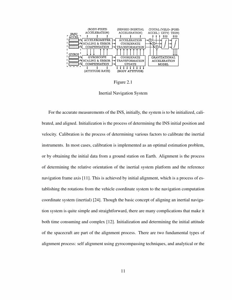
Figure 2.1

Inertial Navigation System

For the accurate measurements of the INS, initially, the system is to be initialized, cali-

brated, and aligned. Initialization is the process of determining the INS initial position and

velocity. Calibration is the process of determining various factors to calibrate the inertial

instruments. In most cases, calibration is implemented as an optimal estimation problem,

or by obtaining the initial data from a ground station on Earth. Alignment is the process

of determining the relative orientation of the inertial system platform and the reference

navigation frame axis [11]. This is achieved by initial alignment, which is a process of es-

tablishing the rotations from the vehicle coordinate system to the navigation computation

coordinate system (inertial) [24]. Though the basic concept of aligning an inertial naviga-

tion system is quite simple and straightforward, there are many complications that make it

both time consuming and complex [12]. Initialization and determining the initial attitude

of the spacecraft are part of the alignment process. There are two fundamental types of

alignment process: self alignment using gyrocompassing techniques, and analytical or the

11

alignment of slave system with respect to a master system. (See references [11], [12], [24],

[25] for more details).

The advantages of an INS are that it is extremely simple in concept, completely au-

tonomous and self contained, and since most of the error characteristics of the system are

known, they can be modeled easily. However, the inertial navigation systems suffer from

the disadvantage of integration drift, wherein small errors in the measurement of accelera-

tion and angular velocity are integrated into progressively larger errors in velocity, which

are compounded into still greater errors in position. Since the new position is calculated

from the previous calculated position and the measured acceleration and angular velocity,

the mean-squared navigation errors of the system increase with time. Also, the INS is

complex in execution and is expensive [22].

The disadvantage of the increase in the mean-squared error can be avoided by integrat-

ing the INS with other aiding sensors or navigation systems, so as to make corrections to

the measurements of the INS and avoid the integration drift. Such navigation systems are

called aided or integrated navigation systems [12].

2.2.1 Classification of INS

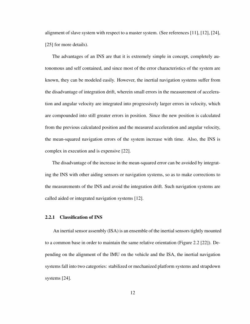
An inertial sensor assembly (ISA) is an ensemble of the inertial sensors tightly mounted

to a common base in order to maintain the same relative orientation (Figure 2.2 [22]). De-

pending on the alignment of the IMU on the vehicle and the ISA, the inertial navigation

systems fall into two categories: stabilized or mechanized platform systems and strapdown

systems [24].

12

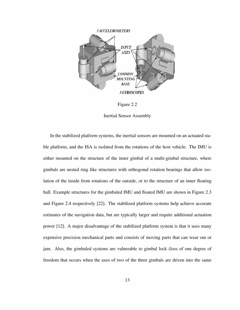
Figure 2.2

Inertial Sensor Assembly

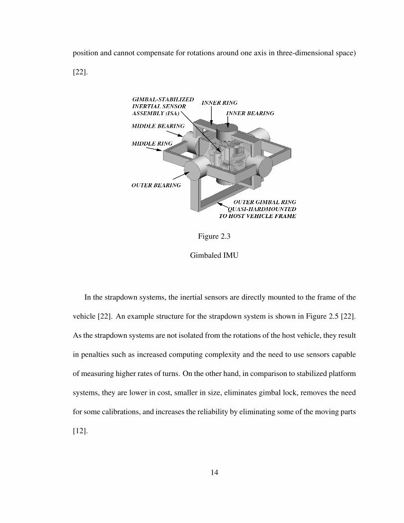
In the stabilized platform systems, the inertial sensors are mounted on an actuated sta-

ble platform, and the ISA is isolated from the rotations of the host vehicle. The IMU is

either mounted on the structure of the inner gimbal of a multi-gimbal structure, where

gimbals are nested ring like structures with orthogonal rotation bearings that allow iso-

lation of the inside from rotations of the outside, or to the structure of an inner floating

ball. Example structures for the gimbaled IMU and floated IMU are shown in Figure 2.3

and Figure 2.4 respectively [22]. The stabilized platform systems help achieve accurate

estimates of the navigation data, but are typically larger and require additional actuation

power [12]. A major disadvantage of the stabilized platform system is that it uses many

expensive precision mechanical parts and consists of moving parts that can wear out or

jam. Also, the gimbaled systems are vulnerable to gimbal lock (loss of one degree of

freedom that occurs when the axes of two of the three gimbals are driven into the same

13

position and cannot compensate for rotations around one axis in three-dimensional space)

[22].

Figure 2.3

Gimbaled IMU

In the strapdown systems, the inertial sensors are directly mounted to the frame of the

vehicle [22]. An example structure for the strapdown system is shown in Figure 2.5 [22].

As the strapdown systems are not isolated from the rotations of the host vehicle, they result

in penalties such as increased computing complexity and the need to use sensors capable

of measuring higher rates of turns. On the other hand, in comparison to stabilized platform

systems, they are lower in cost, smaller in size, eliminates gimbal lock, removes the need

for some calibrations, and increases the reliability by eliminating some of the moving parts

[12].

14

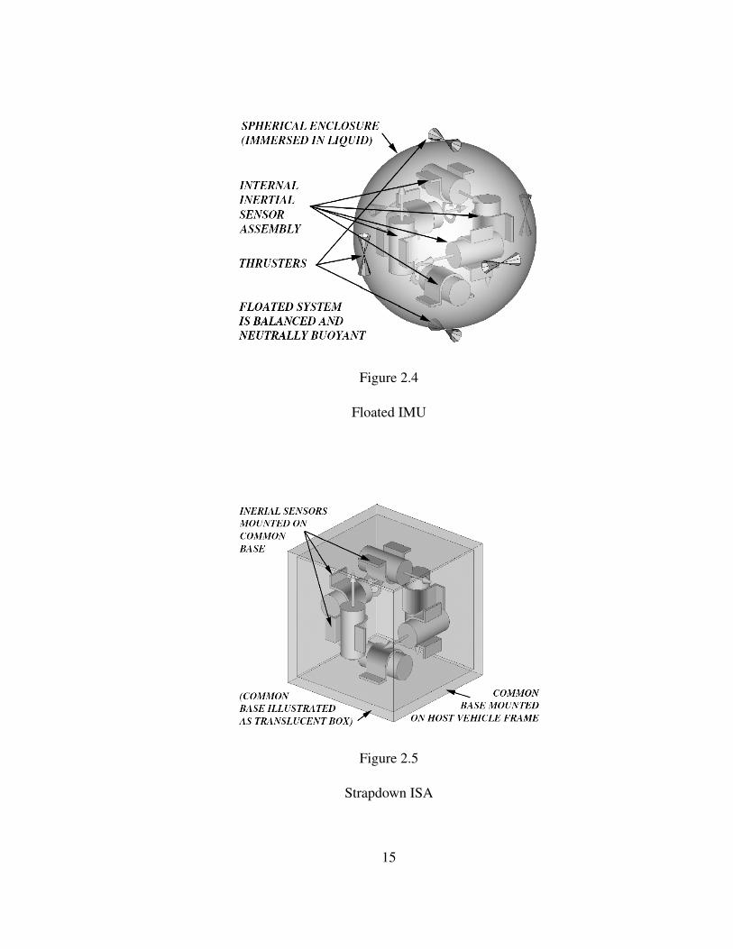
Figure 2.4

Floated IMU

Figure 2.5

Strapdown ISA

15

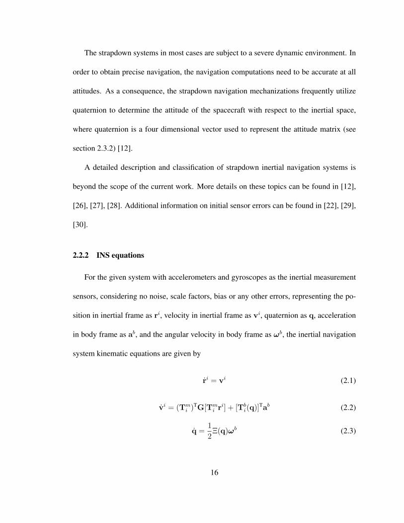
The strapdown systems in most cases are subject to a severe dynamic environment. In

order to obtain precise navigation, the navigation computations need to be accurate at all

attitudes. As a consequence, the strapdown navigation mechanizations frequently utilize

quaternion to determine the attitude of the spacecraft with respect to the inertial space,

where quaternion is a four dimensional vector used to represent the attitude matrix (see

section 2.3.2) [12].

A detailed description and classification of strapdown inertial navigation systems is

beyond the scope of the current work. More details on these topics can be found in [12],

[26], [27], [28]. Additional information on initial sensor errors can be found in [22], [29],

[30].

2.2.2 INS equations

For the given system with accelerometers and gyroscopes as the inertial measurement

sensors, considering no noise, scale factors, bias or any other errors, representing the po-

sition in inertial frame as ri, velocity in inertial frame as vi, quaternion as q, acceleration

in body frame as ab, and the angular velocity in body frame as ωb, the inertial navigation

system kinematic equations are given by

ri = vi (2.1)

vi = (Tmi )

TG[Tmi r

i] + [Tbi(q)]

Tab (2.2)

q =1

2Ξ(q)ωb (2.3)

16

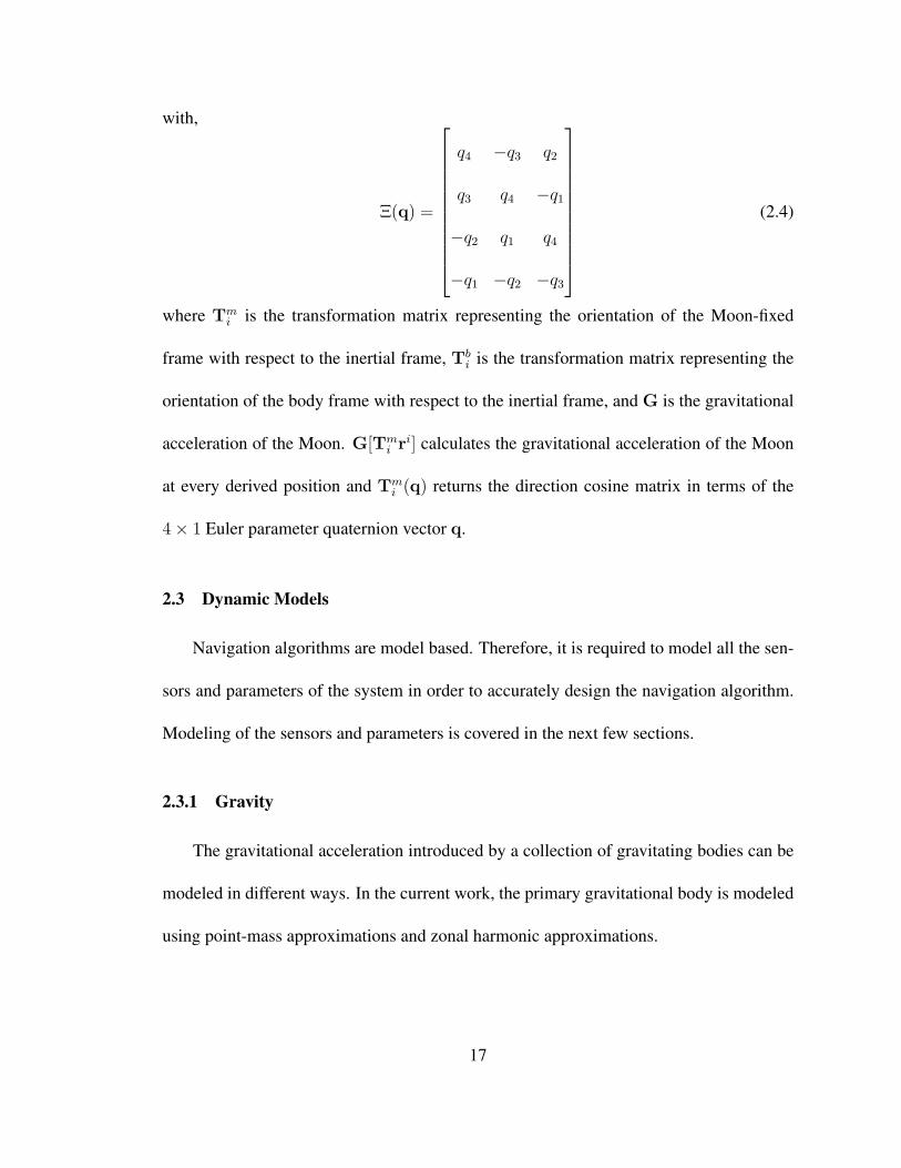
with,

Ξ(q) =

q4 −q3 q2

q3 q4 −q1

−q2 q1 q4

−q1 −q2 −q3

(2.4)

where Tmi is the transformation matrix representing the orientation of the Moon-fixed

frame with respect to the inertial frame, Tbi is the transformation matrix representing the

orientation of the body frame with respect to the inertial frame, and G is the gravitational

acceleration of the Moon. G[Tmi r

i] calculates the gravitational acceleration of the Moon

at every derived position and Tmi (q) returns the direction cosine matrix in terms of the

4× 1 Euler parameter quaternion vector q.

2.3 Dynamic Models

Navigation algorithms are model based. Therefore, it is required to model all the sen-

sors and parameters of the system in order to accurately design the navigation algorithm.

Modeling of the sensors and parameters is covered in the next few sections.

2.3.1 Gravity

The gravitational acceleration introduced by a collection of gravitating bodies can be

modeled in different ways. In the current work, the primary gravitational body is modeled

using point-mass approximations and zonal harmonic approximations.

17

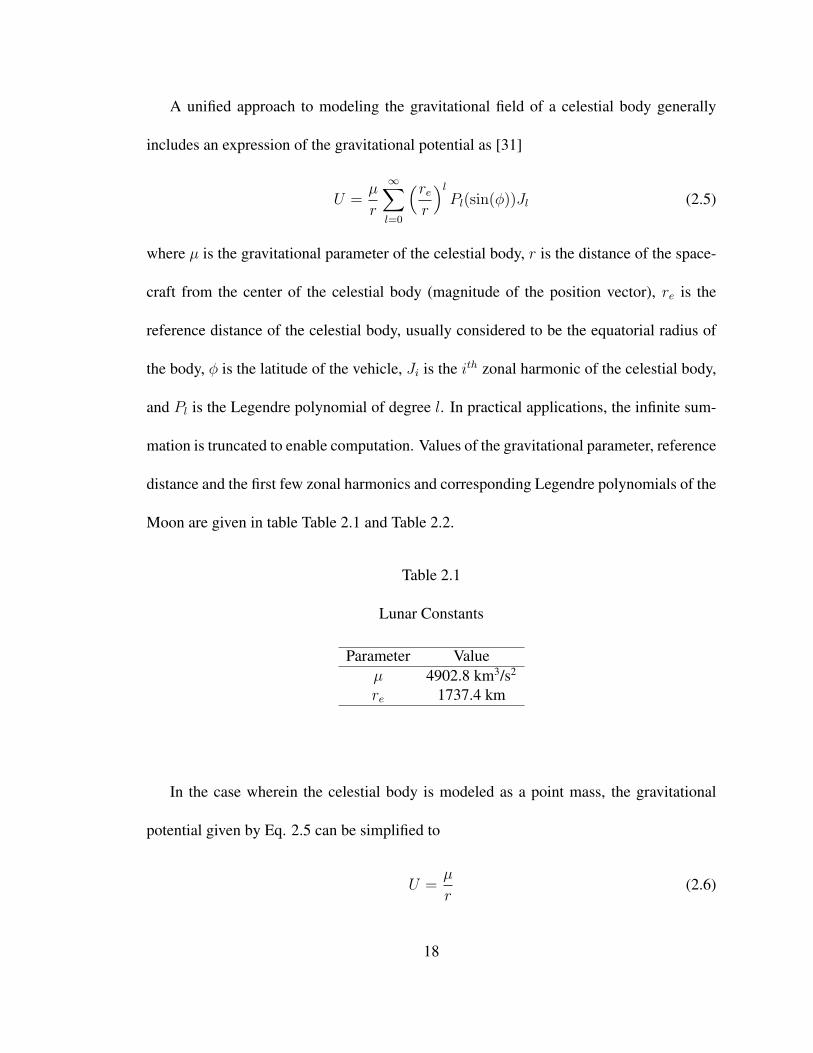
A unified approach to modeling the gravitational field of a celestial body generally

includes an expression of the gravitational potential as [31]

U =µ

r

∞∑l=0

(rer

)l

Pl(sin(ϕ))Jl (2.5)

where µ is the gravitational parameter of the celestial body, r is the distance of the space-

craft from the center of the celestial body (magnitude of the position vector), re is the

reference distance of the celestial body, usually considered to be the equatorial radius of

the body, ϕ is the latitude of the vehicle, Ji is the ith zonal harmonic of the celestial body,

and Pl is the Legendre polynomial of degree l. In practical applications, the infinite sum-

mation is truncated to enable computation. Values of the gravitational parameter, reference

distance and the first few zonal harmonics and corresponding Legendre polynomials of the

Moon are given in table Table 2.1 and Table 2.2.

Table 2.1

Lunar Constants

Parameter Valueµ 4902.8 km3/s2

re 1737.4 km

In the case wherein the celestial body is modeled as a point mass, the gravitational

potential given by Eq. 2.5 can be simplified to

U =µ

r(2.6)

18

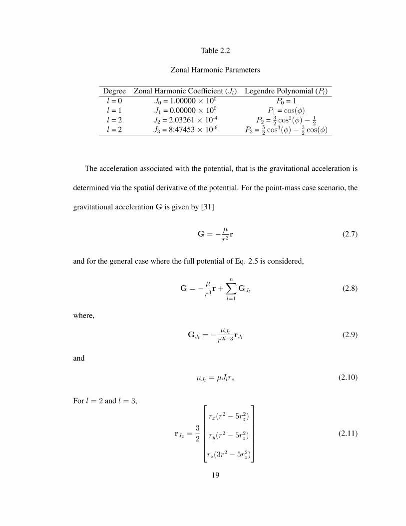
Table 2.2

Zonal Harmonic Parameters

Degree Zonal Harmonic Coefficient (Jl) Legendre Polynomial (Pl)l = 0 J0 = 1.00000 × 100 P0 = 1l = 1 J1 = 0.00000 × 100 P1 = cos(ϕ)l = 2 J2 = 2.03261 × 10-4 P2 = 3

2cos2(ϕ)− 1

2

l = 2 J3 = 8:47453 × 10-6 P3 = 52cos3(ϕ)− 3

2cos(ϕ)

The acceleration associated with the potential, that is the gravitational acceleration is

determined via the spatial derivative of the potential. For the point-mass case scenario, the

gravitational acceleration G is given by [31]

G = − µ

r3r (2.7)

and for the general case where the full potential of Eq. 2.5 is considered,

G = − µ

r3r+

n∑l=1

GJl (2.8)

where,

GJl = − µJl

r2l+3rJl (2.9)

and

µJl = µJlre (2.10)

For l = 2 and l = 3,

rJ2 =3

2

rx(r

2 − 5r2z)

ry(r2 − 5r2z)

rz(3r2 − 5r2z)

(2.11)

19

rJ3 =1

2

5rxrz(3r

2 − 7r2z)

5ryrz(3r2 − 7r2z)

5r2z(6r2 − 7r2z)− 3r4

(2.12)

where rx, ry and rz are the components of the position vector in each direction, such that

r = [rx ry rz] and r =√r2x + r2y + r2z .

2.3.2 Attitude Quaternion Kinematics

The attitude of a vehicle is defined as its orientation with respect to a defined frame of

reference. The vehicle body coordinate system and the reference frame coordinate system

are two frames usually defined to describe the attitude. For most dynamical applications,

these coordinate systems have orthogonal unit vectors that follow the right-hand rule [32].

The attitude matrix of a vehicle, defined by A, mapping from the reference frame to the

body frame is given by

B = AR (2.13)

where B = [Bx By Bz]T is the body frame vector and R = [Rx Ry Rz]

T is the

reference frame vector. The attitude matrix is a real orthogonal matrix.

The attitude matrix can be represented using various parameterizations, like the Euler

angles, Euler axis/angle, the quaternion, Cayley-Klein parameters, Gibb’s vector, etc.

The use of quaternion to determine the attitude of rigid bodies have several advan-

tages over the use of Euler angles or other methods [33]. Quaternions involve the use

of algebraic equations to determine the elements of the attitude matrix, instead of using

trigonometric functions and involve fewer multiplications to propagate successive incre-

20

mental rotations. Therefore, the computations are faster and also there are no singularities

involved [32].

The quaternion is a four dimensional vector defined as

q =

ϱ

q4

(2.14)

with

ϱ = [q1 q2 q3]T = e sin(θ/2) (2.15)

q4 = cos(θ/2) (2.16)

where θ is the rotation angle about ϱ. The quaternion components cannot be independent

of each other as a four-dimensional vector is being used to describe three dimensions, and

therefore satisfies a single constraint given by qTq = 1 [32]. The attitude matrix in terms

of the quaternion is given by

A(q) = ΞT(q)Ψ(q) (2.17)

with

Ξ(q) =

q4I3×3 + [ϱ×]

−ϱ×

(2.18)

Ψ(q) =

q4I3×3 − [ϱ×]

−ϱ×

(2.19)

where [ϱ×] is referred to as a cross product matrix given by

[ϱ×] =

0 −q3 q2

q3 0 −q1

−q2 q1 0

(2.20)

21

Quaternion multiplication and quaternion inverse are defined as

q′ ⊗ q = [Ψ(q′) q′]q = [Ξ(q) q]q′ (2.21)

q−1 =

−ϱ

q4

(2.22)

If δq is the error in the quaternion measurement, the multiplicative error quaternion in

body frame is given by

δq = q⊗ q−1 (2.23)

Defining ω as the angular velocity vector of the body frame relative to the reference

frame, the quaternion kinematics equation is given by [34]

q =1

2Ξ(q)ω =

1

2Ω(ω)q (2.24)

where

Ω(ω) =

−[ω×] ω

−ωT 0

(2.25)

2.4 IMU Sensor Models

The accelerometers and gyroscopes together form the inertial measurement unit (IMU).

Apart from the accelerometers and gyroscopes, the IMU may also include other compo-

nents. A brief on the working of mechanical accelerometers and gyroscopes, and their

models is now discussed.

2.4.1 Accelerometers

An accelerometer is a device which uses the inertia of mass to measure the difference

between the kinematic acceleration with reference to the inertial space and the accelera-22

tion due to gravity [24]. In simple terms, it is a device which measures the acceleration

experienced by a body relative to freefall.

An accelerometer works based on Newton’s second law of motion, which states that

a force F acting on a body of mass m causes the body to accelerate with respect to in-

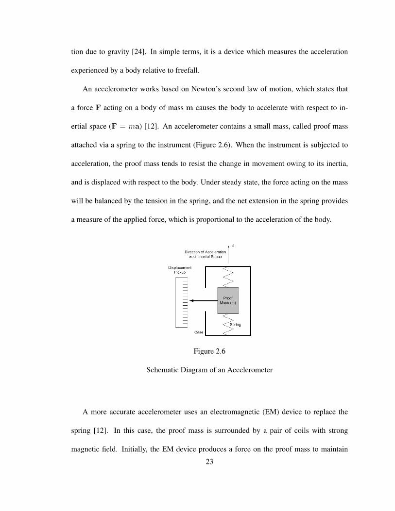
ertial space (F = ma) [12]. An accelerometer contains a small mass, called proof mass

attached via a spring to the instrument (Figure 2.6). When the instrument is subjected to

acceleration, the proof mass tends to resist the change in movement owing to its inertia,

and is displaced with respect to the body. Under steady state, the force acting on the mass

will be balanced by the tension in the spring, and the net extension in the spring provides

a measure of the applied force, which is proportional to the acceleration of the body.

Figure 2.6

Schematic Diagram of an Accelerometer

A more accurate accelerometer uses an electromagnetic (EM) device to replace the

spring [12]. In this case, the proof mass is surrounded by a pair of coils with strong

magnetic field. Initially, the EM device produces a force on the proof mass to maintain

23

it at its null position, and when a deflection is sensed, an electric current is produced in

the coils to force the return of the proof mass to its null position. The magnitude of the

current in the coils is proportional to the specific force applied on the body, which is in

turn proportional to the acceleration.

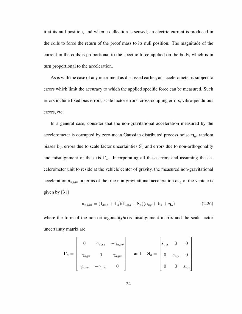
As is with the case of any instrument as discussed earlier, an accelerometer is subject to

errors which limit the accuracy to which the applied specific force can be measured. Such

errors include fixed bias errors, scale factor errors, cross-coupling errors, vibro-pendulous

errors, etc.

In a general case, consider that the non-gravitational acceleration measured by the

accelerometer is corrupted by zero-mean Gaussian distributed process noise ηa, random

biases ba, errors due to scale factor uncertainties Sa and errors due to non-orthogonality

and misalignment of the axis Γa. Incorporating all these errors and assuming the ac-

celerometer unit to reside at the vehicle center of gravity, the measured non-gravitational

acceleration ang,m in terms of the true non-gravitational acceleration ang of the vehicle is

given by [31]

ang,m = (I3×3 + Γa)(I3×3 + Sa)(ang + ba + ηa) (2.26)

where the form of the non-orthogonality/axis-misalignment matrix and the scale factor

uncertainty matrix are

Γa =

0 γa,xz −γa,xy

−γa,yz 0 γa,yx

γa,zy −γa,zx 0

and Sa =

sa,x 0 0

0 sa,y 0

0 0 sa,z

24

From 2.26, the true non-gravitational acceleration ang is given as

ang = (I3×3 + Sa)−1(I3×3 + Γa)

−1ang,m − ba − ηa (2.27)

Note that the acceleration measured by the accelerometer does not include the gravita-

tional acceleration and is therefore denoted as non-gravitational acceleration.

2.4.2 Gyroscopes

A gyroscope is a device which measures the angular velocity and the orientation of a

body. It works on the basic principle of conservation of angular momentum, where angular

momentum of a rotating body is defined as the product of its moment of inertia and angular

velocity [12]. It is also based on the principle that a spinning wheel in the absence of

torque, maintains the direction of its spin axis, and in presence of torque, rotates in the

direction tending to align the spin axis with the input torque axis [24].

The gyroscope consists of a wheel, called gyro wheel, mounted in an axle supported

by fixed bearings on an inner gimbal, placed in an outer gimbal as seen in Figure 2.7. In

practical applications, the gyros are classified into two types: free gyros and restrained

gyros [35].

In free gyros, there are no restraining forces in any direction of the gyro and the gyro

wheel remains fixed in space. The angular moment of the supporting frame is not trans-

mitted to the gyro wheel and hence, the gyroscope measures the angular motions of the

vehicle with respect to the instrument as reference.

25

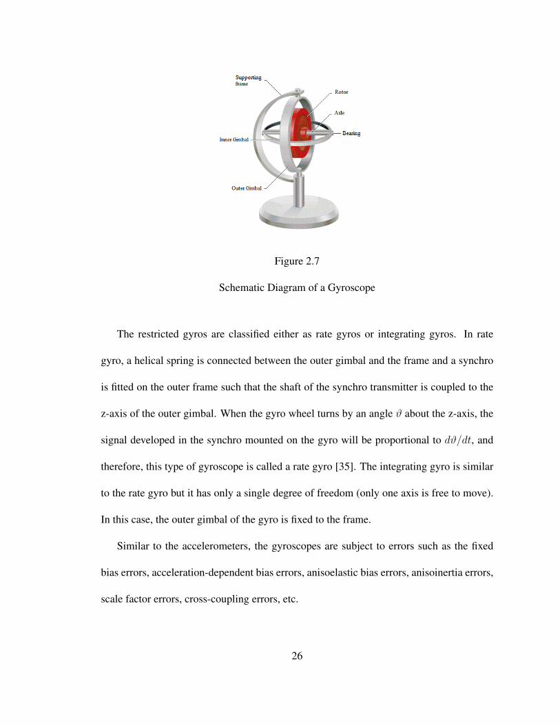
Figure 2.7

Schematic Diagram of a Gyroscope

The restricted gyros are classified either as rate gyros or integrating gyros. In rate

gyro, a helical spring is connected between the outer gimbal and the frame and a synchro

is fitted on the outer frame such that the shaft of the synchro transmitter is coupled to the

z-axis of the outer gimbal. When the gyro wheel turns by an angle ϑ about the z-axis, the

signal developed in the synchro mounted on the gyro will be proportional to dϑ/dt, and

therefore, this type of gyroscope is called a rate gyro [35]. The integrating gyro is similar

to the rate gyro but it has only a single degree of freedom (only one axis is free to move).

In this case, the outer gimbal of the gyro is fixed to the frame.

Similar to the accelerometers, the gyroscopes are subject to errors such as the fixed

bias errors, acceleration-dependent bias errors, anisoelastic bias errors, anisoinertia errors,

scale factor errors, cross-coupling errors, etc.

26

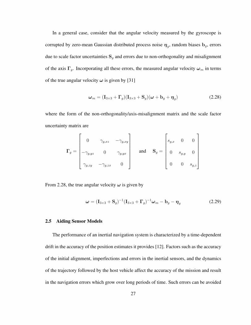
In a general case, consider that the angular velocity measured by the gyroscope is

corrupted by zero-mean Gaussian distributed process noise ηg, random biases bg, errors

due to scale factor uncertainties Sg and errors due to non-orthogonality and misalignment

of the axis Γg. Incorporating all these errors, the measured angular velocity ωm in terms

of the true angular velocity ω is given by [31]

ωm = (I3×3 + Γg)(I3×3 + Sg)(ω + bg + ηg) (2.28)

where the form of the non-orthogonality/axis-misalignment matrix and the scale factor

uncertainty matrix are

Γg =

0 γg,xz −γg,xy

−γg,yz 0 γg,yx

γg,zy −γg,zx 0

and Sg =

sg,x 0 0

0 sg,y 0

0 0 sg,z

From 2.28, the true angular velocity ω is given by

ω = (I3×3 + Sg)−1(I3×3 + Γg)

−1ωm − bg − ηg (2.29)

2.5 Aiding Sensor Models

The performance of an inertial navigation system is characterized by a time-dependent

drift in the accuracy of the position estimates it provides [12]. Factors such as the accuracy

of the initial alignment, imperfections and errors in the inertial sensors, and the dynamics

of the trajectory followed by the host vehicle affect the accuracy of the mission and result

in the navigation errors which grow over long periods of time. Such errors can be avoided

27

by use of more accurate sensors, but the use of these sensors is limited and also increases

the cost of the system.

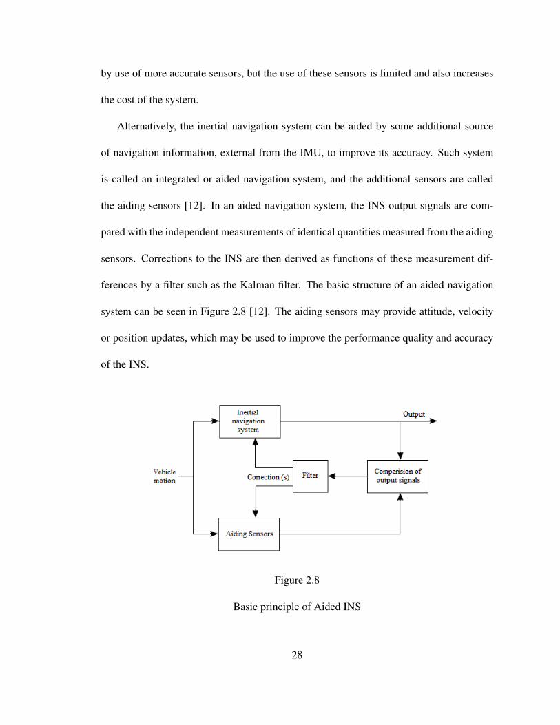
Alternatively, the inertial navigation system can be aided by some additional source

of navigation information, external from the IMU, to improve its accuracy. Such system

is called an integrated or aided navigation system, and the additional sensors are called

the aiding sensors [12]. In an aided navigation system, the INS output signals are com-

pared with the independent measurements of identical quantities measured from the aiding

sensors. Corrections to the INS are then derived as functions of these measurement dif-

ferences by a filter such as the Kalman filter. The basic structure of an aided navigation

system can be seen in Figure 2.8 [12]. The aiding sensors may provide attitude, velocity

or position updates, which may be used to improve the performance quality and accuracy

of the INS.

Figure 2.8

Basic principle of Aided INS

28

The navigation aids or aiding sensors can be categorized into external measurements

and on-board measurements. External measurements are the measurements obtained by

receiving signals or data from outside the vehicle. Examples are radio navigation aids,

satellites, star trackers, ground-based radar trackers, etc. On-board measurements are mea-

surements derived using additional sensors carried on-board the spacecraft. Examples are

altimeter, Doppler radar, radar or electro-optical imaging systems, etc.

For the current thesis, an altimeter, a terrain camera and a star camera are used as the

aiding sensors. More on the sensors and their models is now discussed.

2.5.1 Altimeter

An altimeter is an instrument used to measure the altitude of an object above a fixed

level. There are three major types of altimeters: barometric altimeters, radar altimeters,

and lidar altimeters [12].

Barometric altimeters or pressure altimeters measure the atmospheric pressure to in-

directly provide a measure of the altitude of the vehicle above a nominal sea level, up to

an error of less than 0.01 percent. Barometric altimeters are mostly used in inertial sys-

tems requiring three-dimensional navigation systems to restrict the growth of errors in the

vertical channel of the INS. Typically, barometric altimeters are not applicable for lunar

landing problems due to low atmospheric pressure on the Moon.

A radar altimeter is a more direct measure of measuring the altitude. The radar altime-

ters, as the name indicates, work based on radio detection and ranging (radar) principle.

Radio waves are transmitted towards the body the altitude is to be measured from, and the

29

time it takes for them to be reflected back and return to the vehicle is measured. Since

speed, distance and time are interrelated, the distance or altitude halt from the surface pro-

viding the reflection can be calculated from the velocity of the radio wave vrad and the

time it takes to travel the distance t. (halt = vradt).

Lidar altimeters are optical remote sensing devices working on principle of light de-

tection and ranging, and similar to radar altimeters. Instead of using radio waves, they use

laser pulses to determine the distance from the body.

Considering the general model of an on-board altimeter corrupted by random constant

bias balt, and Gaussian random noise ηalt, the altitude measured halt is given by [31]

halt = halt(rfalt) + balt + ηalt (2.30)

where rfalt is the position of the altimeter in the planet fixed frame.

For the case where the altimeter is measuring the altitude over a spherical body, the

specific altitude measurement is given by [31]

hsph = rialt − rsph + balt + ηalt (2.31)

where rialt is the distance of the altimeter to the surface of the body in the inertial frame,

equal to magnitude of the position vector ∥ rialt ∥, and rsph is the spherical radius of the

body under consideration.

2.5.2 Terrain Camera

Terrain referenced navigation techniques such as terrain contour matching help achieve

the position information of the vehicle [12]. The basic terrain referenced navigation sys-30

tem uses the INS, a radar altimeter and a stored contour map of the area over which the

vehicle is flying. The information of the altitude measurements from the altimeter and the

estimates from INS allow the a reconstruction of the ground profile beneath the flight path

on the on-board computer. The resulting profile is then compared with the stored map data

to get a fix on the position of the vehicle. The accuracy of the position fix obtained is a

function of the roughness of the terrain.

The accuracy of the terrain referenced or terrain contour matching navigation can be

improved by using more precise sensors such as image based sensors. A camera in the

terrain referenced navigation, called terrain camera, provides the precise position of the

vehicle. The terrain cameras take pictures of certain feature points on the terrain of the

planetary body the vehicle is flying over. To obtain the position information, the image

taken is converted to an array of pixels, each pixel having a numerical value indicating

the brightness of that part of the image. The image is then processed to remove noise

and enhance its features. Then a correlation algorithm is used to search for recognizable

patterns, which appear in a pre-stored database of the ground features. Once a match for

the image is found in the database, geometrical calculations based on the vehicles altitude

and attitude enable the determination of its position [12].

The terrain camera output corrupted by random bias btc and Gaussian random noise

ηtc is given by [31]

utc = Tbi(q)rtc + btc + ηtc (2.32)

31

where rtc is the terrain camera position with reference to a feature point at position rfp

such that

rtc = r− rfp (2.33)

where rfp is assumed to be known.

2.5.3 Star Camera

A star camera or star tracker is a celestial reference device that recognizes star patterns,

such as constellations [12]. It is an optical device that measures the position of star using

either photocells or a camera. The star camera locates the positions of stars by capturing

images and these captured images are compared to a celestial map that resides in the

spacecraft computer memory to determine the location of the spacecraft.

The star camera is either used to measure the position or the attitude of the vehicle. To

estimate the position of the spacecraft using star sightings or celestial observations, sight-

ings of stars are achieved to provide measurements of the azimuth and elevation angles of

the star with respect to a known reference frame within the vehicle. These measurements

are then compared with the predictions of the same quantities derived from knowledge of

the declination and sidereal hour angle of the star [12].

Using star cameras, the attitude of the spacecraft can be determined either by vector

measurement models, maximum likelihood estimations or by optimal quaternion solution

using Euler angle parameterizations of the attitude matrix. If the measured stars can be

identified as specific cataloged stars, then the attitude matrix can be determined from the

32

measured stars in image coordinates and identified stars in inertial coordinates using the

nonlinear least squares approach [32].

Considering the star camera to measure the quaternion, the output of a star camera is

given by

qsc = q (2.34)

Allowing the measurement of the quaternion to be potentially corrupted by a random bias

bsc, and a white-noise process ηsc, a bias-noise quaternion can be formed as [31]

qb,η =

sin(θsc2

)θsc

θsc

cos(θsc2

) (2.35)

where θsc = bsc + ηsc and θsc =∥ θsc ∥. Assuming small angles, Eq. 2.35 can be written

as

qb,η =

12θsc

1

(2.36)

In terms of the error quaternion and the measurement frame quaternion, the star camera

output can be given as

qsc = qb,η ⊗ q (2.37)

33

CHAPTER 3

KALMAN FILTERING

3.1 Kalman Filter

A Kalman filter can be defined as an optimal recursive data processing algorithm

[36]. It processes all the given measurements using prior knowledge of the system and

measuring device dynamics, to estimate the current values of the desired variables while

minimizing the errors statistically. In order to achieve this, it also makes use of the statis-

tical description of measurement and system noises, uncertainties in the dynamic models,

and any available initial conditions. One of the main advantages of using a Kalman filter

is its recursiveness, which means that there is no need to store past measurement data and

reprocess it every time for computing the present estimates.

A Kalman filter can also be defined as an estimator of the linear-quadratic problem

[37]. The linear-quadratic problem is the problem of estimating the instantaneous state of

a linear dynamic system perturbed by Gaussian white noise using measurements that are

linear functions of the system state corrupted by noise. A Kalman filter has two major

applications: estimating the state of the dynamic systems and performance analysis of the

dynamic systems; and is used for the analysis of measurement and estimation problems.

The goal of the Kalman filter is to find the best estimate xk of the state vector from the

measurements up to and including time tk.

34

The Kalman filter has many applications in the inertial navigation systems. It is used

for the initialization of the INS to determine the initial position and velocity, and also to

integrate the measurements of the aiding sensors with the estimates of the INS, and make

the necessary corrections in the position, velocity and attitude estimates of the spacecraft.

Being a recursive technique, it is particularly suitable for on-line estimations, which lends

itself to implementations in a computer [12].

The principles of Kalman filtering are now described.

3.1.1 Covariance

Covariance is a measure of how much two variables change together. The random state

and forcing function vectors are generally described in terms of their covariance matrices

[38]. The error x in the estimate of a state vector is defined to be the difference between

the estimated value x and actual value x, such that [32]

x = x− x (3.1)

The covariance of x, designated by P is given by

P = E[xxT] (3.2)

where E[x] is the expected value of x.

The covariance matrix provides a statistical measure of the uncertainties in x. The

covariance matrix of an n-state vector is always an n×n symmetric matrix and the diagonal

elements are the mean square error in terms of the state variables.

35

3.1.2 Continuous-Discrete Kalman Filter

The continuous-time Kalman filter is not widely used in practice today due to the

extensive use of digital computers. However, the discrete-time and continuous-discrete-

time Kalman filter are widely used for most of the applications [32]. The continuous-

discrete-time systems are dynamical systems which include a continuous-time model with

discrete-time measurements taken from a digital signal processor.

The system and measurement model for the continuous-discrete-time system are given

by

x(t) = F (t)x(t) +B(t)u(t) +G(t)w(t) (3.3)

yk = Hkxk + vk (3.4)

The continuous-time covariance of w(t) is given by

Ew(t)w(τ)T = Q(t)δ(t− τ) (3.5)

and the discrete-time covariance of vk is given by

EvkvTj =

0 k = j

Rk k = j

(3.6)

where,

x(t) is the state vector

yk is the measurement or observation vector

u(t) is the control vector

w(t) is the process noise

36

v(t) is the observation noise

F (t) is the state transition matrix

B(t) is the control input matrix

G(t) is the process noise input matrix

Hk is the measurement sensitivity matrix or observation matrix

Q(t) is the covariance of dynamic disturbance noise

Rk is the covariance of sensor noise or measurement uncertainty

δ(t− τ) is a dirac-delta function

For the continuous-discrete-time Kalman filter, at a given time t1, the state estimate

model is first propagated until a measurement occurs, then a discrete-time state update

occurs, which updates the final value of the propagated state x−1 to new state x+

1 . This

state is then used as the initial condition to propagate the state estimate model to time t2

and the process continues forward in time, updating the state when a measurement occurs

[32].

Initializing x(t0) = x0 and P0 = Ex(t0)xT(t0), the equations for the continuous-

discrete Kalman filter for the model described are given by [32]

Kalman Gain:

Kk = P−kH

Tk [HkP

−kH

Tk +Rk]

−1 (3.7)

Measurement Update:

x+k = x−

k +Kk[yk −Hkx−k ] (3.8)

P+k = [I −KkHk]P

−k (3.9)

37

Propagation:

˙x(t) = F (t)x(t) +B(t)u(t) (3.10)

P(t) = F (t)P(t) +P(t)F T(t) +G(t)Q(t)F T(t) (3.11)

where,

Kk is the Kalman gain.

P−k is the predicted or a priori value of estimation covariance

P+k is the corrected or a posteriori value of estimation covariance

x−k is the predicted or a priori value of the estimated state vector

x+k is the corrected or a posteriori value of the estimated state vector

For the continuous-discrete Kalman filter, the sample times of measurements need not

occur at regular intervals but can be spread over various time intervals and it can therefore

handle different scattered measurement sets.

In conclusion, the Kalman filter can be described as an optimal filter for systems de-

scribed by a linear model with measurement and process noises described by Gaussian

white noises. But for cases with a nonlinear model, the Kalman filter is not applicable,

and large classes of estimation problems involve nonlinear models. A filter applicable for

such nonlinear models is described next.

3.2 Extended Kalman Filter

An extension of the optimal linear Kalman filter is the Extended Kalman Filter (EKF).

The EKF is a recursive data processing algorithm which can combine measurements from

various asynchronous sources with time-varying noise characteristics and is applicable to

38

nonlinear models [32]. The EKF, unlike the Kalman filter utilizes prior knowledge of the

state and error statistics of the system and is model-dependent, thus the accurate modeling

of the sensors is important for proper functioning of the filter. For the nonlinear models,

the EKF utilizes the notion that the true state is sufficiently close to the estimated state.

The measurement and system model are estimated by describing the error dynamics using

a linearized first-order Taylor series expansion. The extended Kalman filter, though not

precisely optimum, has been applied successfully to various nonlinear systems [32].

3.2.1 Continuous-Discrete Extended Kalman Filter

Consider a continuous-discrete time systems given by

x(t) = f(x(t),u(t), t) +G(t)w(t) (3.12)

yk = h(xk) + vk (3.13)

where,

f is the dynamic model function

h is the measurement function

Initializing x(t0) = x0 and P0 = Ex(t0)xT(t0), the extended Kalman filter equa-

tions for the continuous-discrete time system are given by [32]

Kalman Gain:

Kk = P−kH

Tk (x

−k )[Hk(x

−k )P

−kH

Tk (x

−k ) +Rk]

−1 (3.14)

Hk(x−k ) ≡

∂h

∂x|x−

k(3.15)

39

Measurement Update:

x+k = x−

k +Kk[yk − h(x−k )] (3.16)

P+k = [I −KkHk(x

−k )]P

−k (3.17)

Propagation:

˙x(t) = f(x(t),u(t), t) (3.18)

P(t) = F (x(t), t)P(t) +P(t)F T(x(t), t) +G(t)Q(t)GT(t) (3.19)

F (x(t), t) =∂f

∂x|x(t) (3.20)

From the equations above, it can be seen that when the system dynamics and measure-

ments are linear, the extended Kalman filter reduces to a conventional Kalman filter.

Though the EKF with all its advantages has been the most popular method for non

linear estimation to this day, it does have a few disadvantages. Such flaws and a method

to overcome them are described in the next section.

3.3 Unscented Kalman Filter

In general, the problem of filtering nonlinear dynamic models is more difficult in

comparison to the case of linear models. The extended Kalman filters typically works well

only in the region where the first-order Taylor series expansion approximates the nonlinear

probability distribution i.e. where the true state is close to the estimated state [32]. In

cases where the initial estimated state is far from the true state, this assumption leads to

instabilities in the filter. To overcome this disadvantage of the EKF, various extensions

40

of the Kalman filter for the nonlinear model have been developed to achieve improved

performance, but most came at the cost of increased computational burden.

One such extension of the Kalman filter for nonlinear models called the unscented or

sigma-point Kalman filter (UKF) was developed by Julier, Uhlmann, and Durant-White.

The UKF is an alternative filter which overcomes the disadvantages of the Extended

Kalman filter (EKF) while achieving superior performance and with the computational

complexity equal to that of the EKF [39]. Few advantages of the UKF over EKF are

described below [32].

• The expected error of UKF is lower than the EKF.

• UKF is applicable to non-differentiable functions.

• UKF avoids the derivation of the Jacobian matrices.

• UKF is valid for higher-order expansions than the standard EKF.

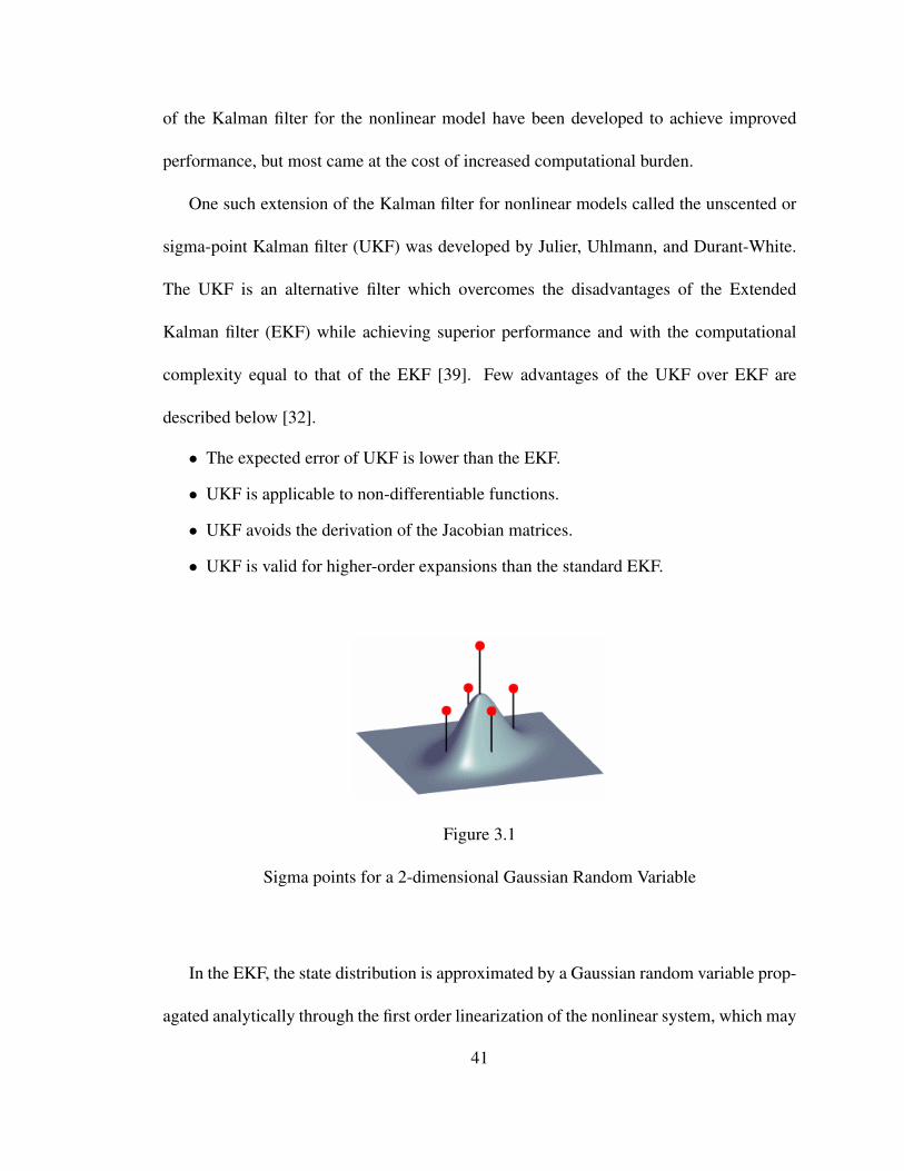
Figure 3.1

Sigma points for a 2-dimensional Gaussian Random Variable

In the EKF, the state distribution is approximated by a Gaussian random variable prop-

agated analytically through the first order linearization of the nonlinear system, which may

41

introduce large errors in the true mean and covariance of the transformed random variable

and lead to sub-optimal performance and diverge the filter [39]. The UKF, on the other

hand uses a deterministic sampling approach wherein the state distribution approximated

by the Gaussian random variable is represented using a minimal set of sample points called

the Sigma points (Figure 3.1 [40]) which capture the true mean and covariance of the ran-

dom variable. These sigma points when propagated through the true nonlinear system

completely capture the posterior mean and the covariance of the random variable accu-

rately to the second order for any nonlinearity. The basic sigma-point approach can be

described as [40]

• A set of weighted samples which capture the first and second order moments ofthe prior random variable, called the sigma-points are deterministically calculatedusing the mean and square root decomposition of the covariance matrix of the priorrandom variable.

• These sigma-points are propagated through the true nonlinear function using func-tional evaluations.

• The posterior statistics are approximated using tractable functions of the the propa-gated sigma-points and weights.

In comparison to the general stochastic sampling techniques such as the Monte-Carlo

integration which requires large number of sample points in order to accurately propa-

gate the state, the sigma-point filter uses fewer sample points to approximate the prop-

agated state to the third order for Gaussian inputs, and at least to the second order for

non-Gaussian inputs for all nonlinearities. And as mentioned above, the UKF does not

involve the calculations of analytical Jacobian matrices unlike the EKF. This makes the

sigma-point approach very attractive for use in black box systems where analytical ex-

42

pressions of the system dynamics are either not available or not in a form which allows for

easy linearization [39].

3.3.1 Unscented Transformation

The unscented transformation is a method for calculating the statistics of a random

variable undergoing nonlinear transformation [39]. Consider a random variable x of di-

mension L, mean x and covariance Px propagated through a nonlinear function y = f(x).

The statistics of the function y are calculated by forming a matrix X of 2L+1 sigma vec-

tors X i, such that

X 0 = x (3.21)

X i = x+ (√

(L+ λ)Px)i i = 1, . . . , L (3.22)

X i = x− (√

(L+ λ)Px)i−L i = L+ 1, . . . , 2L (3.23)

where λ = α2(L + κ) − L is a scaling parameter, wherein α determines the extent of

spread of sigma points around the prior mean x, and κ is a secondary scaling parameter.

Typical values of the scaling factors are 1e − 3 < α ≤ 1 and κ = 0, and in general, their

optimal values are problem specific.

The sigma vectors calculated are propagated through the nonlinear function

Y i = f(X i) i = 0, . . . , 2L (3.24)

and the mean and covariance for y are approximated using a weighted sample mean and

covariance of the posterior sigma points

y ≈2L∑i=0

W(m)i Y i (3.25)

43

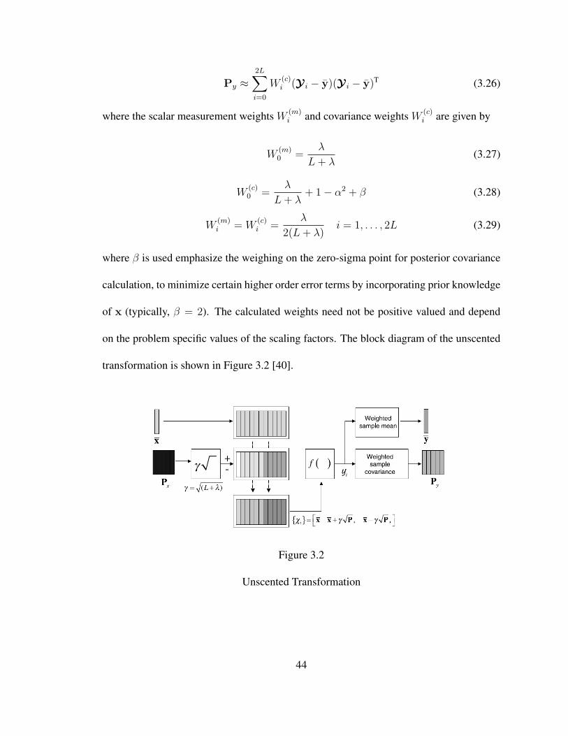
Py ≈2L∑i=0

W(c)i (Y i − y)(Y i − y)T (3.26)

where the scalar measurement weights W (m)i and covariance weights W (c)

i are given by

W(m)0 =

λ

L+ λ(3.27)

W(c)0 =

λ

L+ λ+ 1− α2 + β (3.28)

W(m)i = W

(c)i =

λ

2(L+ λ)i = 1, . . . , 2L (3.29)

where β is used emphasize the weighing on the zero-sigma point for posterior covariance

calculation, to minimize certain higher order error terms by incorporating prior knowledge

of x (typically, β = 2). The calculated weights need not be positive valued and depend

on the problem specific values of the scaling factors. The block diagram of the unscented

transformation is shown in Figure 3.2 [40].

Figure 3.2

Unscented Transformation

44

3.3.2 Unscented Kalman Filter

The unscented Kalman filter is a straightforward extension of the unscented transfor-

mation to the recursive estimation, where the random variable is redefined as the concen-

tration of the original state and noise variables [39]. For a discrete time nonlinear dynamic

system

xk+1 = F(xk,uk,wk) (3.30)

yk = H(xk,vk) (3.31)

the augmented state is given by

xak = [xT

k wTk vT

k ]T (3.32)

where,

wk is the Gaussian process noise

vk is the Gaussian observation noise

Initializing x(t0) = x0, P0 = Ex(t0)xT(t0) and calculating the augmented state

vector and covariance matrix

xa0 = Exa =

[xT0 0 0

]T

Pa0 = Exa

0 xa T0 =

P0 0 0

0 Q 0

0 0 R

for k ∈ 1, . . . ,∞, the sigma points can be calculated as [39]

X ak−1 =

[xak−1 xa

k−1 + γ√

Pak−1 xa

k−1 − γ√

Pak−1

](3.33)

45

Once the sigma points are calculated, the equations for the unscented Kalman filter are

given by [39]

Time Update:

X xk|k−1 = F(X x

k−1,uk−1,Xwk−1) (3.34)

x−k =

2L∑i=0

W(m)i X i,k|k−1 (3.35)

P−k =

2L∑i=0

W(c)i (X i,k|k−1 − x−

k )(X i,k|k−1 − x−k )

T (3.36)

Measurement Update:

Yk|k−1 = H(X xk|k−1,X v

k−1) (3.37)

y−k =

2L∑i=0

W(m)i Y i,k|k−1 (3.38)

Pykyk=

2L∑i=0

W(c)i (Y i,k|k−1 − y−

k )(Y i,k|k−1 − y−k )

T (3.39)

Pxkyk=

2L∑i=0

W(c)i (X i,k|k−1 − x−

k )(Y i,k|k−1 − y−k )

T (3.40)

Kalman Gain:

Kk = PxkykP−1

ykyk(3.41)

Propagation:

xk = x−k +Kk(yk − y−

k ) (3.42)

Pk = P−k −KkPykyk

KTk (3.43)

where, X a = [(X x)T (Xw)T (X v)T]T, γ =√

(L+ λ), λ is the composite scaling

parameter, L is the dimension of the augmented state, Q is the process noise covariance,

R is the measurement noise covariance, and Wi are the weights.46

Even though propagations on the order of 2L are required, the computations are com-

parable to the extended Kalman filter. For cases wherein the measurement noise vk ap-

pears linearly in the output, the augmented state can be reduced as the system state need

not be augmented with the measurement noise. In such case, the covariance of the mea-

surement error Rk is added to the innovations covariance Pykyk. This can greatly reduce

the computational requirements of the unscented Kalman filter [32].

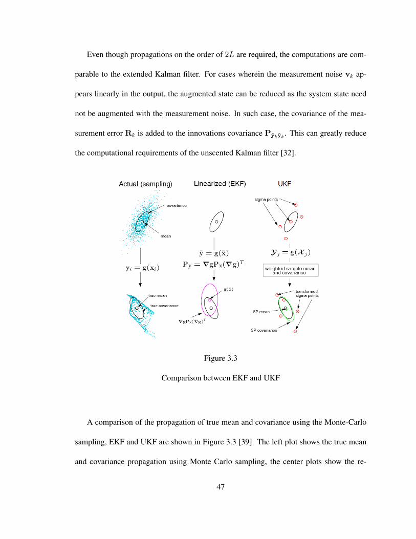
Figure 3.3

Comparison between EKF and UKF

A comparison of the propagation of true mean and covariance using the Monte-Carlo

sampling, EKF and UKF are shown in Figure 3.3 [39]. The left plot shows the true mean

and covariance propagation using Monte Carlo sampling, the center plots show the re-

47

sults using the EKF, and the right hand plots show the performance of the UKF. From

observation, it can be concluded that the UKF achieves better performance than the EKF.

3.4 Application of Kalman Filter to Aided INS

The Kalman filtering technique provides a means of using measurements from aiding

sensors to improve the high accuracy inertial navigation performance [24] and is a well

established technique for the mixing of navigation data in integrated systems.

Kalman filtering involves the combination of two estimates of a variable to form a

weighted mean, where the weighting factors are chosen to yield the most probable es-

timate. One of the two estimates is obtained from the measurement while the other is

provided by updating a previous best estimate in accordance with the known equations of

motion. For an integrated navigation system, the first estimate is provided by the measure-

ment aid while the second is provided by the INS measurement, where the inertial system

constitutes the model of the physical process that produces the measurement [12].

Since, the inertial system equations and also the measurements provided by the nav-

igation aids are non-linear, a modified filter such as the extended Kalman filter or the

Unscented Kalman filter is used for the integrated navigation systems.

48

CHAPTER 4

NAVIGATION SYSTEM AND ALGORITHM

For a spacecraft making its final descent from a lunar orbit onto the surface of the

Moon, integrating the aiding sensor measurements from the on-board altimeter, terrain

camera and star camera to the measurements of the inertial navigation system using an

unscented Kalman filter, in order to accurately estimate the position, velocity and attitude

of the spacecraft forms the basic navigation algorithm for the current thesis work.

The dynamics of the landing scenario being considered, the block diagram of the nav-

igation system, numerical considerations, filter structure and the unscented Kalman filter

for the INS are now studied.

4.1 Landing Scenario

For a lunar landing problem, a spacecraft from Earth arrives on a hyperbolic trajectory

when viewed from the vicinity of the Moon. The vehicle can either land directly onto

the lunar surface from the orbit, or can enter into a parking orbit around the Moon. For

the current work, a spacecraft descending from a parking orbit onto a safe and precise

lunar landing site is being considered. The landing site is assumed to be chosen using

an accurate landing point designation algorithm [41]. A schematic representation of the

descent-to-landing scenario is demonstrated in Figure 4.1.

49

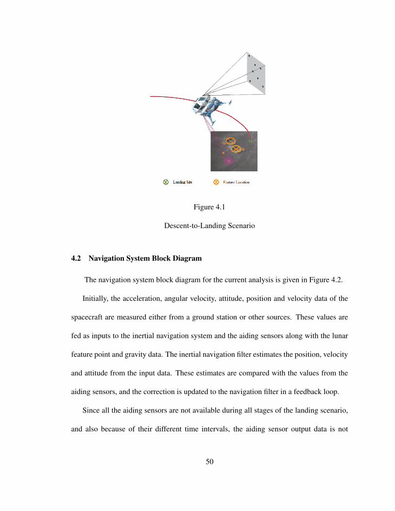
Figure 4.1

Descent-to-Landing Scenario

4.2 Navigation System Block Diagram

The navigation system block diagram for the current analysis is given in Figure 4.2.

Initially, the acceleration, angular velocity, attitude, position and velocity data of the

spacecraft are measured either from a ground station or other sources. These values are

fed as inputs to the inertial navigation system and the aiding sensors along with the lunar

feature point and gravity data. The inertial navigation filter estimates the position, velocity

and attitude from the input data. These estimates are compared with the values from the

aiding sensors, and the correction is updated to the navigation filter in a feedback loop.

Since all the aiding sensors are not available during all stages of the landing scenario,

and also because of their different time intervals, the aiding sensor output data is not

50

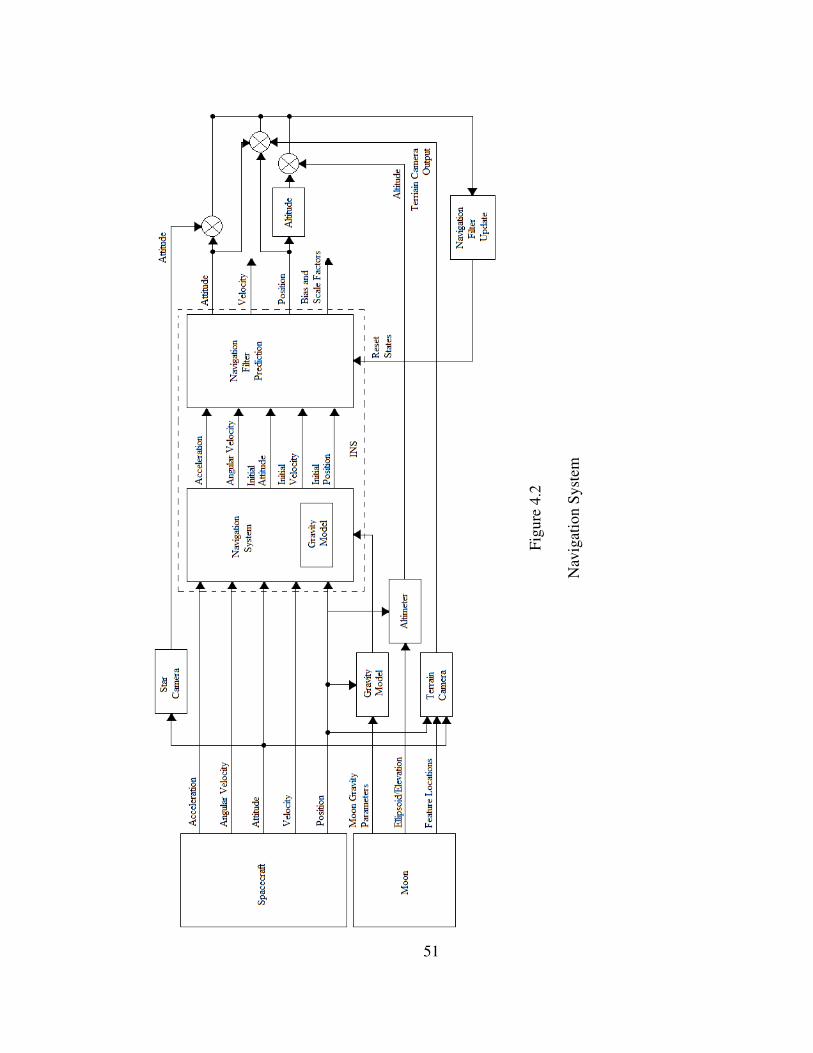
Figu

re4.

2

Nav

igat

ion

Syst

em

51

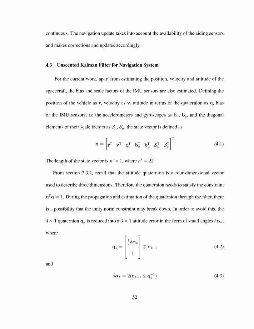
continuous. The navigation update takes into account the availability of the aiding sensors

and makes corrections and updates accordingly.

4.3 Unscented Kalman Filter for Navigation System

For the current work, apart from estimating the position, velocity and attitude of the

spacecraft, the bias and scale factors of the IMU sensors are also estimated. Defining the

position of the vehicle as r, velocity as v, attitude in terms of the quaternion as q, bias

of the IMU sensors, i.e the accelerometers and gyroscopes as ba, bg, and the diagonal

elements of their scale factors as Sa, Sg, the state vector is defined as

x =

[rT vT qT bT

a bTg ST

a STg

]T

(4.1)

The length of the state vector is n′ × 1, where n′ = 22.

From section 2.3.2, recall that the attitude quaternion is a four-dimensional vector

used to describe three dimensions. Therefore the quaternion needs to satisfy the constraint

qTq = 1. During the propagation and estimation of the quaternion through the filter, there

is a possibility that the unity norm constraint may break down. In order to avoid this, the

4× 1 quaternion qk is reduced into a 3× 1 attitude error in the form of small angles δαk,

where

qk =

12δαk

1

⊗ qk−1 (4.2)

and

δαk = 2(qk−1 ⊗ q−1k ) (4.3)

52

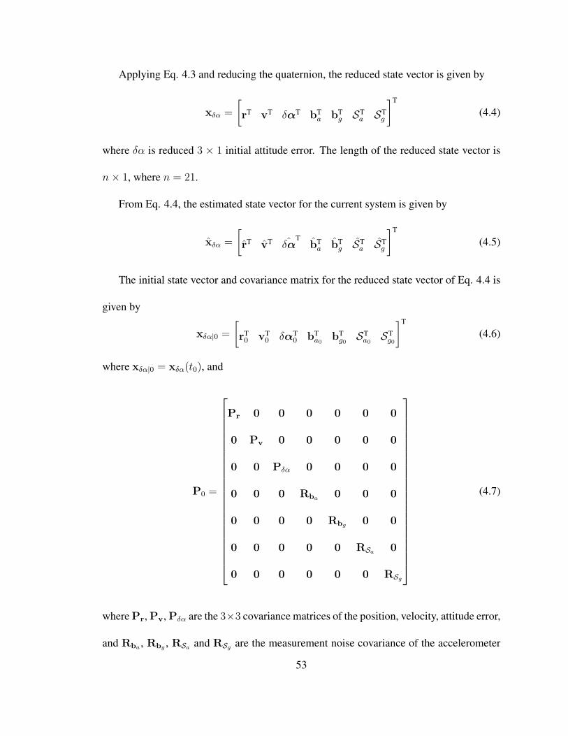
Applying Eq. 4.3 and reducing the quaternion, the reduced state vector is given by

xδα =

[rT vT δαT bT

a bTg ST

a STg

]T

(4.4)

where δα is reduced 3 × 1 initial attitude error. The length of the reduced state vector is

n× 1, where n = 21.

From Eq. 4.4, the estimated state vector for the current system is given by

xδα =

[rT vT ˆδα

TbTa bT

g STa ST

g

]T

(4.5)

The initial state vector and covariance matrix for the reduced state vector of Eq. 4.4 is

given by

xδα|0 =

[rT0 vT

0 δαT0 bT

a0bTg0

STa0

STg0

]T

(4.6)

where xδα|0 = xδα(t0), and

P0 =

Pr 0 0 0 0 0 0

0 Pv 0 0 0 0 0

0 0 Pδα 0 0 0 0

0 0 0 Rba 0 0 0

0 0 0 0 Rbg 0 0

0 0 0 0 0 RSa 0

0 0 0 0 0 0 RSg

(4.7)

where Pr, Pv, Pδα are the 3×3 covariance matrices of the position, velocity, attitude error,

and Rba , Rbg , RSa and RSg are the measurement noise covariance of the accelerometer

53

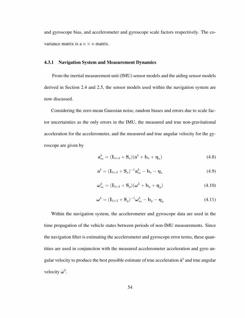
and gyroscope bias, and accelerometer and gyroscope scale factors respectively. The co-

variance matrix is a n× n matrix.

4.3.1 Navigation System and Measurement Dynamics

From the inertial measurement unit (IMU) sensor models and the aiding sensor models

derived in Section 2.4 and 2.5, the sensor models used within the navigation system are

now discussed.

Considering the zero-mean Gaussian noise, random biases and errors due to scale fac-

tor uncertainties as the only errors in the IMU, the measured and true non-gravitational

acceleration for the accelerometer, and the measured and true angular velocity for the gy-

roscope are given by

abm = (I3×3 + Sa)(a

b + ba + ηa) (4.8)

ab = (I3×3 + Sa)−1ab

m − ba − ηa (4.9)

ωbm = (I3×3 + Sg)(ω

b + bg + ηg) (4.10)

ωb = (I3×3 + Sg)−1ωb

m − bg − ηg (4.11)

Within the navigation system, the accelerometer and gyroscope data are used in the

time propagation of the vehicle states between periods of non-IMU measurements. Since

the navigation filter is estimating the accelerometer and gyroscope error terms, these quan-

tities are used in conjunction with the measured accelerometer acceleration and gyro an-

gular velocity to produce the best possible estimate of true acceleration ab and true angular

velocity ωb.

54

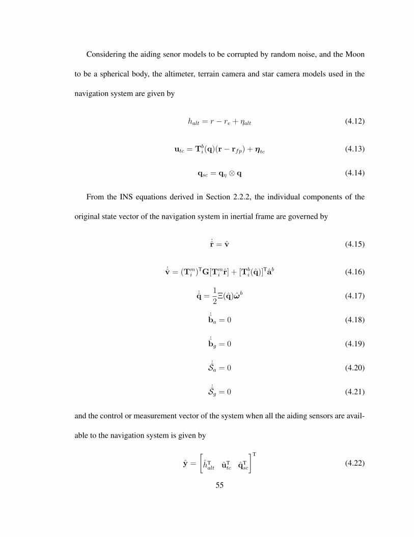
Considering the aiding senor models to be corrupted by random noise, and the Moon

to be a spherical body, the altimeter, terrain camera and star camera models used in the

navigation system are given by

halt = r − re + ηalt (4.12)

utc = Tbi(q)(r− rfp) + ηtc (4.13)

qsc = qη ⊗ q (4.14)

From the INS equations derived in Section 2.2.2, the individual components of the

original state vector of the navigation system in inertial frame are governed by

˙r = v (4.15)

˙v = (Tmi )

TG[Tmi r] + [Tb

i(q)]Tab (4.16)

˙q =1

2Ξ(q)ωb (4.17)

˙ba = 0 (4.18)

˙bg = 0 (4.19)

˙Sa = 0 (4.20)

˙Sg = 0 (4.21)

and the control or measurement vector of the system when all the aiding sensors are avail-

able to the navigation system is given by

y =

[hTalt uT

tc qTsc

]T

(4.22)

55

where,

ab = (I3×3 + Sa)−1ab

m − ba (4.23)

ωb = (I3×3 + Sg)−1ωb

m − bg (4.24)

h = r − re (4.25)

utc = Tbi(q)(r− rfp) (4.26)

qsc = q (4.27)

4.3.2 Sigma Points

In order to calculate the sigma points, the augmented state vector and covariance

matrix need to be calculated. The augmented reduced state vector for the current system

is given by

xaδα|0 =

[xTδα|0 0 0 0

]T

(4.28)

where xδα|0 is the estimated reduced state vector, and the zero vectors are the process

noises of the accelerometer (3 × 1), gyroscope (3 × 1) and their bias and scale factors

(12 × 1) respectively. The length of the augmented reduced state vector is l × 1, where

l = n+ 3 + 3 + 12 = 39.

The augmented covariance matrix is given by

Pa0 =

P0 0 0 0

0 Qa 0 0

0 0 Qg 0

0 0 0 Qb,S

(4.29)

56

where Qa, Qg, Qb,S are the process noise covariances of the accelerometer, gyroscope

and their bias and scale factors respectively. The size of the augmented covariance matrix

is l × l.

Using the augmented reduced state vector and covariance matrix, the sigma points are

calculated from

X aδα|k−1 =

[xaδα|k−1 xa

δα|k−1 + γ√

Pak−1 xa

δα|k−1 − γ√Pa

k−1

](4.30)

This sigma point matrix is for the reduced state vector and is a l×(2l+1) matrix where the

first n× (2l + 1) elements represent the reduced state vector, and the remaining elements

represent the process noise. In order to obtain the sigma points for the original state vector,

an attitude perturbation is performed using Eq. 4.2 to change the 3×1 attitude error sigma

points to 4× 1 quaternion sigma points.

X ak−1 =

[X aT

δα|k−1(1:6)X aT

q|k−1 X aT

δα|k−1(11:n′)

]T

(4.31)

where X aq|k−1 is a 4× (2l+1) matrix and X a

δα|k−1(1:6), X a

δα|k−1(11:n′)represent rows 1 to 6,

and 11 to n′ of the augmented reduced sigma point matrix. Here, rows 1 to 3, 4 to 6, and

7 to 10 of the sigma point matrix represent the sigma points corresponding the position,

velocity, and the quaternion respectively, and are denoted as X r, X v and X q, while rows

11 to n′ represent the sigma points of the navigation errors.

4.3.3 Propagation and Update without Measurements

Assuming the case where none of the aiding sensor measurements are available to the

navigation filter, and that the navigation update does not occur, the sigma points of Eq.57

4.31 are propagated through the navigation system dynamic Eqs. 4.15 - 4.21 using the

Runge-Kutta integration method [17] as

r = v

v = (Tmi )

TG[Tmi r] + [Tb

i(q)]Tab

q =1

2Ξ(q)ωb

ba = 0 bg = 0 Sa = 0 Sg = 0

where,

r = X r v = X v q = X q

Since the propagated sigma points are for the original state vector, the 4×1 quaternion

sigma points are reduced to 3×1 attitude error sigma points using Eq. 4.3. The propagated

reduced sigma points are given as

X k|δα =

[X T

k(1:6)X T

δα|k X Tk(10:n)

]T

(4.32)

where X δα|k is a 3× (2l + 1) matrix.

In order to update the state vector and covariance, the scalar measurement and co-

variance weights need to be calculated. Using optimal values of ψ, β and κ, the weights

are

W(m)0 =

λ

l + λ(4.33)

W(c)0 =

λ

l + λ+ 1− ψ2 + β (4.34)

W(m)i =W

(c)i =

λ

2(l + λ)i = 1, . . . , 2l (4.35)

58

where, λ = ψ2√l + κ− l.

The updated reduced state and covariance estimates are then calculated from the prop-

agated reduced sigma points, such that

x−δα|k =

2l∑i=0

W(m)i X δα|ki (4.36)

P−k =

2l∑i=0

W(c)i (X δα|ki − x−

δα|k)(X δα|ki − x−δα|k)

T (4.37)

Since there is no measurement update, a priori state estimate and a priori covariance

obtained from Eq. 4.36 and Eq. 4.37 are the estimated state vector and covariace of the

navigation system.

xδα|k = x−δα|k (4.38)

Pk = P−k (4.39)

Changing the reduced state vector to its original form through attitude perturbation

using Eq. 4.2, the state estimate vector is

xk =

[xTδα|k(1:6) qT

k xTδα|k(11:n′)

]T

(4.40)

where qk is the 4× 1 quaternion estimate.

4.3.4 Propagation and Update with Measurements

The case where at least one of the aiding sensor measurement is available to the

navigation filter is now discussed. As mentioned earlier, the navigation filter is capable of

accounting and updating the filter for cases where one, two or all the three aiding sensor

measurements are available.59

To obtain a measurement update, the sigma points calculated from Eq. 4.31 need to

be propagated through the measurement control vector of Eq. 4.22. Reducing the 4 × 1

output measurement of the star camera to a 3 × 1 vector using Eq. 4.3, the measurement

control vector when all aiding sensors are available is given by

yδα|k =

[hTalt|k uT

tc|k qTsc|δα|k

](4.41)

For the model described in section 2.5.1, the altimeter measurement sigma points Yalt

are calculated from the sigma points corresponding to the position X r and the spherical

radius of the Moon re as

Yalt|k = ∥X r|k∥ − re (4.42)

For the model described in section 2.5.2, the terrain camera measurement sigma points

Y tc calculated from the sigma points corresponding to the position X r and quaternion X q

are given by

Y tc|k = Tbi(X q|k)(X r|k − rfp|k) (4.43)

where rfp is the position of the feature point on the surface of the Moon.

From the model described in section 2.5.3, the star camera measurement sigma points

Ysc are calculated using the sigma points corresponding to the quaternion X q as

Ysc|k = X q|k (4.44)

Using Eq. 4.3, the 4 × (2l + 1) star camera measurement sigma points is reduced to

3× (2l + 1) matrix Ysc|δα|k.

60

Considering all the three aiding sensors measurements to be available, the measure-

ment sigma points are given by

Yδα|k =

[YT

alt|k YTtc|k YT

sc|δα|k

]T

(4.45)

To obtain a priori measurement estimate and measurement covariance matrix, the mea-

surement sigma points are propagated through

y−δα|k =

2l∑i=0

W(m)i Yδα|ki (4.46)

Pykyk=

2l∑i=0

W(c)i (Yδα|ki − y−

k )(Yδα|ki − y−k )

T +

Ralt 0 0

0 Rtc 0

0 0 Rsc

(4.47)

Using a priori state estimate calculated in Eq. 4.36, the cross covariance matrix is

calculated as

Pxkyk=

2l∑i=0

W(c)i (X δα|ki − x−

δα|k)(Yδα|ki − y−δα|k)

T (4.48)

The Kalman gain is given by

Kk = PxkykP−1

ykyk(4.49)

The estimated reduced state vector and covariance matrix are then calculated using the

Kalman gain as

xδα|k = x−δα|k +Kk(yδα|k − y−

δα|k) (4.50)

Pk = P−k −KkPykyk

KTk (4.51)

61

Calculating the original state vector from the reduced state vector of Eq. 4.50 using

Eq. 4.2, the state estimate update vector for the navigation filter is given by

xk =

[xTδα|k1:6 qT

k xTδα|k11:n′

]T

(4.52)

62

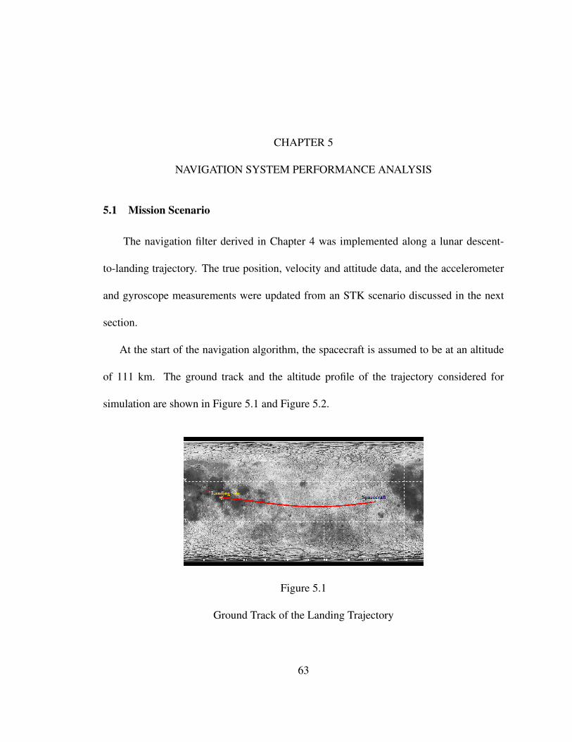
CHAPTER 5

NAVIGATION SYSTEM PERFORMANCE ANALYSIS

5.1 Mission Scenario

The navigation filter derived in Chapter 4 was implemented along a lunar descent-

to-landing trajectory. The true position, velocity and attitude data, and the accelerometer

and gyroscope measurements were updated from an STK scenario discussed in the next

section.

At the start of the navigation algorithm, the spacecraft is assumed to be at an altitude

of 111 km. The ground track and the altitude profile of the trajectory considered for

simulation are shown in Figure 5.1 and Figure 5.2.

Figure 5.1

Ground Track of the Landing Trajectory

63

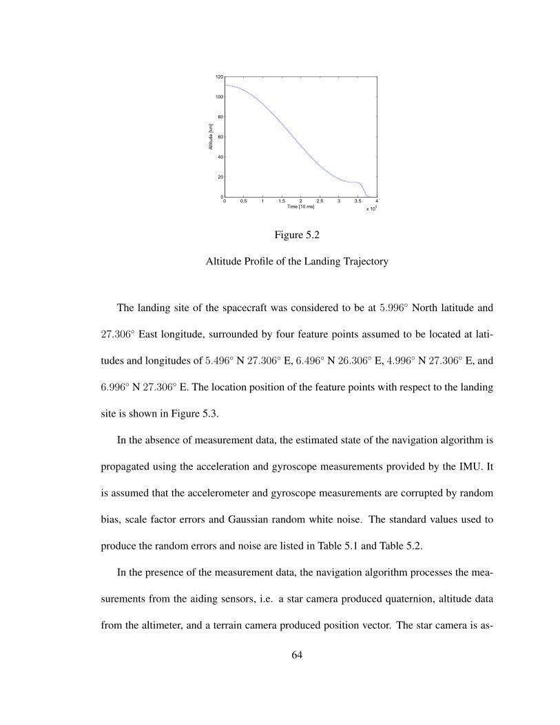
0 0.5 1 1.5 2 2.5 3 3.5 4

x 105

0

20

40

60

80

100

120

Alti

tude

[km

]Time [10 ms]

Figure 5.2

Altitude Profile of the Landing Trajectory

The landing site of the spacecraft was considered to be at 5.996 North latitude and

27.306 East longitude, surrounded by four feature points assumed to be located at lati-

tudes and longitudes of 5.496 N 27.306 E, 6.496 N 26.306 E, 4.996 N 27.306 E, and

6.996 N 27.306 E. The location position of the feature points with respect to the landing

site is shown in Figure 5.3.

In the absence of measurement data, the estimated state of the navigation algorithm is

propagated using the acceleration and gyroscope measurements provided by the IMU. It

is assumed that the accelerometer and gyroscope measurements are corrupted by random

bias, scale factor errors and Gaussian random white noise. The standard values used to

produce the random errors and noise are listed in Table 5.1 and Table 5.2.

In the presence of the measurement data, the navigation algorithm processes the mea-

surements from the aiding sensors, i.e. a star camera produced quaternion, altitude data

from the altimeter, and a terrain camera produced position vector. The star camera is as-

64

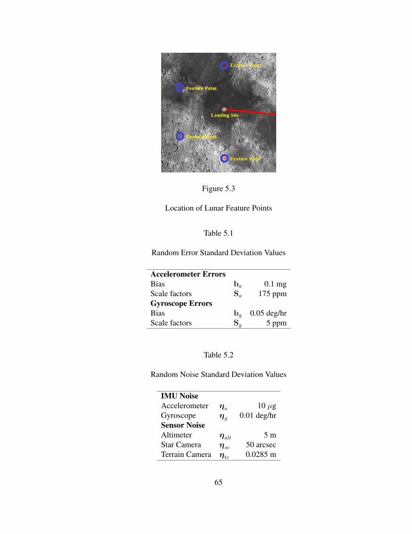
Figure 5.3

Location of Lunar Feature Points

Table 5.1

Random Error Standard Deviation Values

Accelerometer ErrorsBias ba 0.1 mgScale factors Sa 175 ppmGyroscope ErrorsBias bg 0.05 deg/hrScale factors Sg 5 ppm

Table 5.2

Random Noise Standard Deviation Values

IMU NoiseAccelerometer ηa 10 µgGyroscope ηg 0.01 deg/hrSensor NoiseAltimeter ηalt 5 mStar Camera ηsc 50 arcsecTerrain Camera ηtc 0.0285 m

65

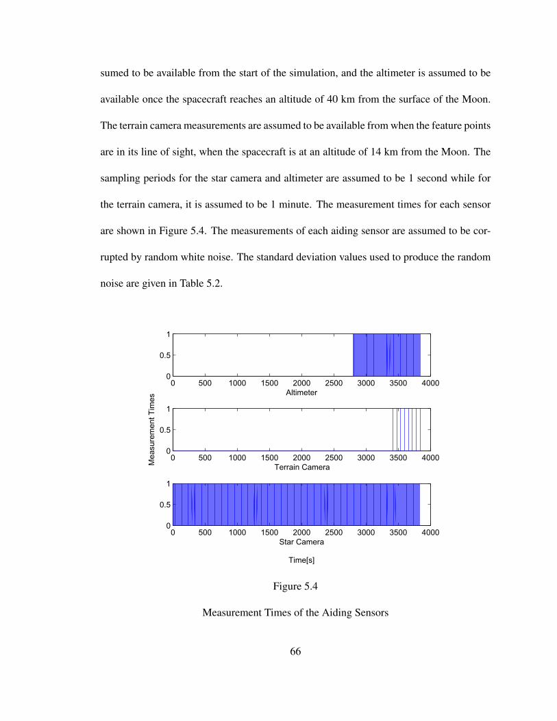
sumed to be available from the start of the simulation, and the altimeter is assumed to be

available once the spacecraft reaches an altitude of 40 km from the surface of the Moon.

The terrain camera measurements are assumed to be available from when the feature points

are in its line of sight, when the spacecraft is at an altitude of 14 km from the Moon. The

sampling periods for the star camera and altimeter are assumed to be 1 second while for

the terrain camera, it is assumed to be 1 minute. The measurement times for each sensor

are shown in Figure 5.4. The measurements of each aiding sensor are assumed to be cor-

rupted by random white noise. The standard deviation values used to produce the random

noise are given in Table 5.2.

0 500 1000 1500 2000 2500 3000 3500 40000

0.5

1

Altimeter

0 500 1000 1500 2000 2500 3000 3500 40000

0.5

1

Terrain CameraMea

sure

men

t Tim

es

0 500 1000 1500 2000 2500 3000 3500 40000

0.5

1

Star Camera

Time[s]

Figure 5.4

Measurement Times of the Aiding Sensors

66

The values of the unscented transformation parameters used for simulation purposes

are listen in Table 5.3

Table 5.3

Unscented Transformation Parameters

Parameter Valueψ 1κ 3 - lβ 2

where l is the length of the augmented state vector (l = 39).

5.2 STK Scenario

The truth data required for the INS to propagate the current estimates for the naviga-

tion system has been obtained from a Kinetic Lunar Lander STK scenario developed by

the Space Exploration Engineering (SEE) Corporation [42]. The data from the scenario

has also been used to compare with the simulated results to determine the accuracy of the

navigation algorithm.

The scenario depicts the landing of a spacecraft from a lunar orbit at an altitude of

111.6 km from the surface of the Moon. The spacecraft takes 1 hour, 16 minutes to land

on the lunar surface from the time of start of descent. Screen captures of the spacecraft

descent-to-landing are presented in Figure 5.5.

67

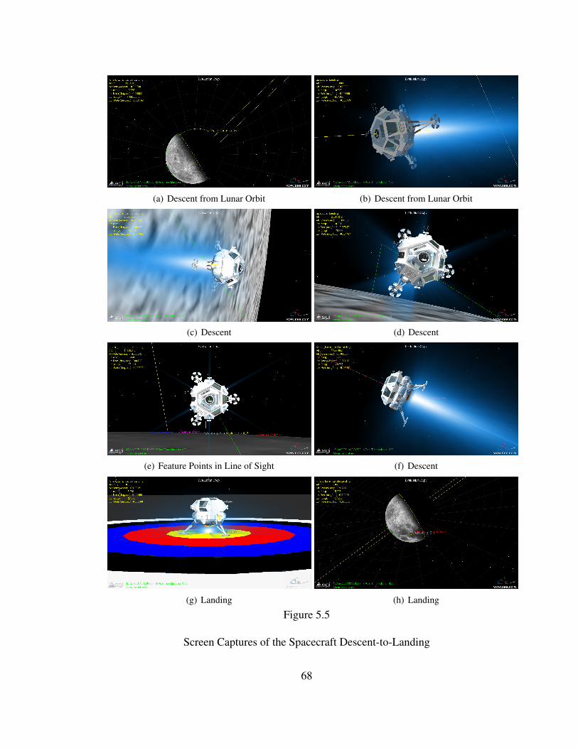
(a) Descent from Lunar Orbit (b) Descent from Lunar Orbit

(c) Descent (d) Descent

(e) Feature Points in Line of Sight (f) Descent

(g) Landing (h) Landing

Figure 5.5

Screen Captures of the Spacecraft Descent-to-Landing

68

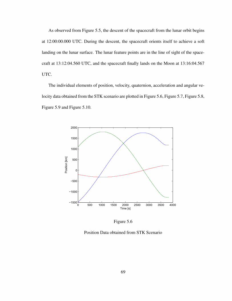
As observed from Figure 5.5, the descent of the spacecraft from the lunar orbit begins

at 12:00:00.000 UTC. During the descent, the spacecraft orients itself to achieve a soft

landing on the lunar surface. The lunar feature points are in the line of sight of the space-

craft at 13:12:04.560 UTC, and the spacecraft finally lands on the Moon at 13:16:04.567

UTC.

The individual elements of position, velocity, quaternion, acceleration and angular ve-

locity data obtained from the STK scenario are plotted in Figure 5.6, Figure 5.7, Figure 5.8,

Figure 5.9 and Figure 5.10.

0 500 1000 1500 2000 2500 3000 3500 4000−1500

−1000

−500

0

500

1000

1500

2000

Time [s]

Pos

ition

[km

]

Figure 5.6

Position Data obtained from STK Scenario

69

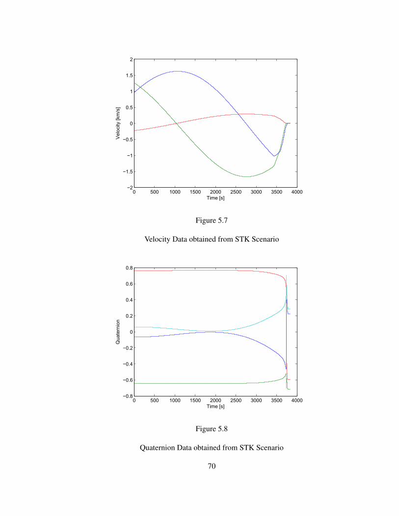
0 500 1000 1500 2000 2500 3000 3500 4000−2

−1.5

−1

−0.5

0

0.5

1

1.5

2

Time [s]

Vel

ocity

[km

/s]

Figure 5.7

Velocity Data obtained from STK Scenario

0 500 1000 1500 2000 2500 3000 3500 4000−0.8

−0.6

−0.4

−0.2

0

0.2

0.4

0.6

0.8

Time [s]

Qua

tern

ion

Figure 5.8

Quaternion Data obtained from STK Scenario

70

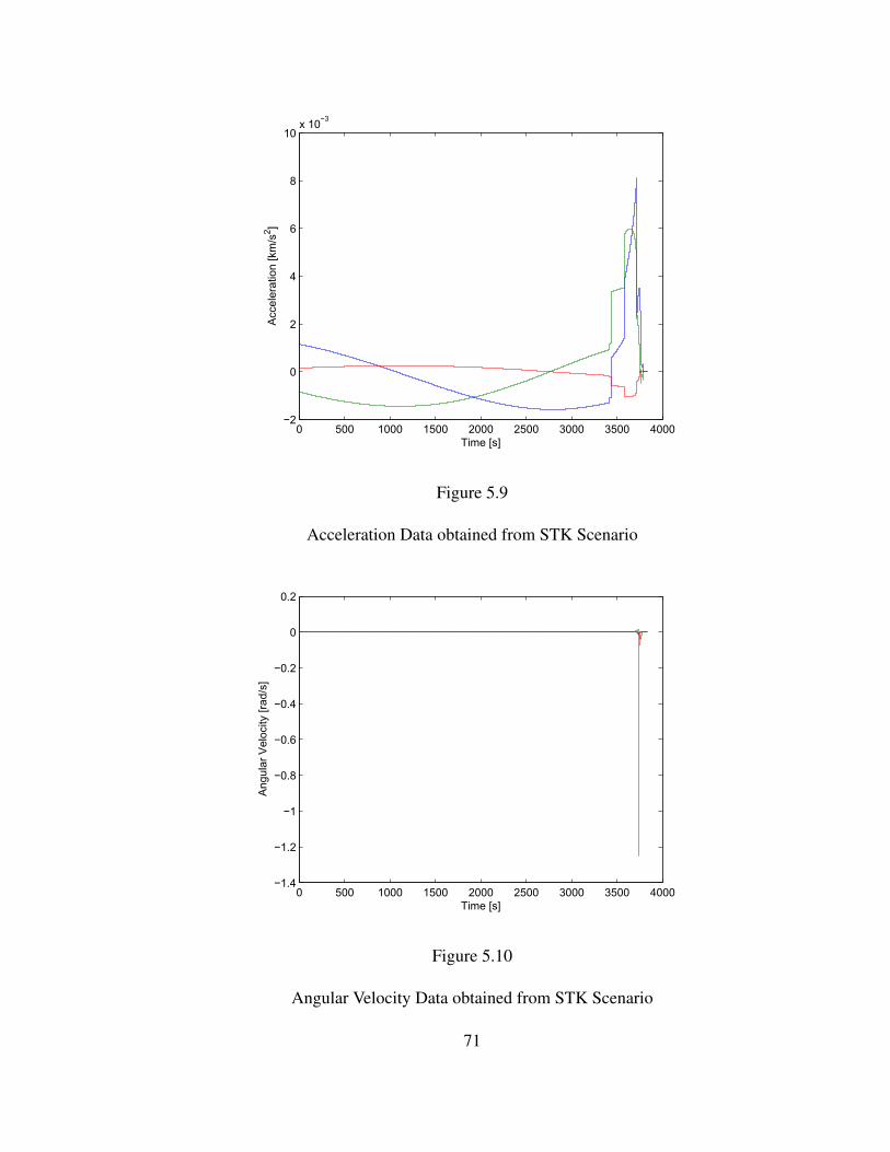
0 500 1000 1500 2000 2500 3000 3500 4000−2

0

2

4

6

8

10x 10

−3

Time [s]

Acc

eler

atio

n [k

m/s

2 ]

Figure 5.9

Acceleration Data obtained from STK Scenario

0 500 1000 1500 2000 2500 3000 3500 4000−1.4

−1.2

−1

−0.8

−0.6

−0.4

−0.2

0

0.2

Time [s]

Ang

ular

Vel

ocity

[rad

/s]

Figure 5.10

Angular Velocity Data obtained from STK Scenario

71

5.3 Estimation Error Results

To verify the functionality of the navigation algorithm developed, a detailed estimation

error analysis was performed for the inertial navigation system and for different combi-

nations of the integrated navigation system. For each case, the state estimation errors are

plotted along with their respective 3σ covariance bounds. The sampling period for the aid-

ing sensor measurements was chosen to be 0.01 seconds, and the initial values of position,

velocity and quaternion were assumed to be noise ridden.

For convenience, the bias and scale factors have been estimated only for the case where

all the three aiding sensor measurements are available to the inertial navigation system and

this system is called the integrated navigation system.

5.3.1 Inertial Navigation System

The navigation filter developed was tested for the inertial navigation system without

any external aiding sensor measurement data. The individual elements of position, velocity

and quaternion state estimation errors with their 3σ covariance bounds are presented in

Figure 5.11, Figure 5.12 and Figure 5.13 (the state estimation error is shown in blue and

the 3σ covariance bounds are shown in red).

From Figure 5.11, it can be observed that without the aiding sensor measurement data,

the position estimation error increases over time to about 6 km at the time of landing.

Similar increase in the velocity and quaternion estimation errors can be observed from

Figure 5.12 and 5.13. This large error in the estimates of the state variable characterizes

the time-dependent integration drift of the inertial navigation system.

72

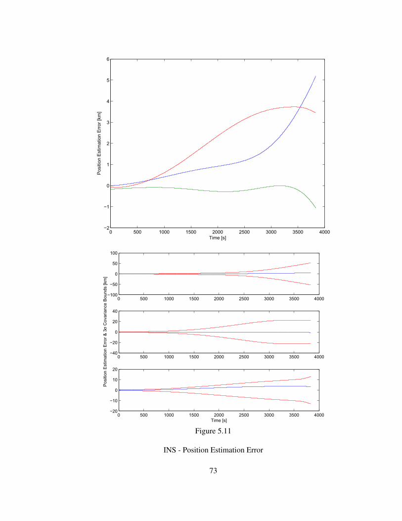
0 500 1000 1500 2000 2500 3000 3500 4000−2

−1

0

1

2

3

4

5

6

Time [s]

Pos

ition

Est

imat

ion

Err

or [k

m]

0 500 1000 1500 2000 2500 3000 3500 4000−100

−50

0

50

100

0 500 1000 1500 2000 2500 3000 3500 4000−40

−20

0

20

40

Pos

ition

Est

imat

ion

Err

or &

3σ

Cov

aria

nce

Bou

nds

[km

]

0 500 1000 1500 2000 2500 3000 3500 4000−20

−10

0

10

20

Time [s]

Figure 5.11

INS - Position Estimation Error

73

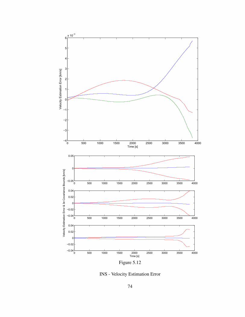
0 500 1000 1500 2000 2500 3000 3500 4000−4

−3

−2

−1

0

1

2

3

4

5

6x 10

−3

Time [s]

Vel

ocity

Est

imat

ion

Err

or [k

m/s

]

0 500 1000 1500 2000 2500 3000 3500 4000−0.05

0

0.05

0 500 1000 1500 2000 2500 3000 3500 4000−0.04

−0.02

0

0.02

0.04

Vel

ocity

Est

imat

ion

Err

or &

3σ

Cov

aria

nce

Bou

nds

[km

/s]

0 500 1000 1500 2000 2500 3000 3500 4000−0.04

−0.02

0

0.02

0.04

Time [s]

Figure 5.12

INS - Velocity Estimation Error

74

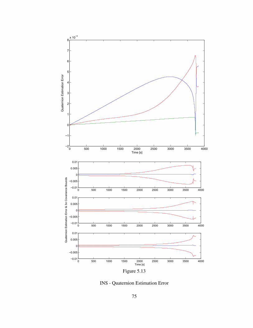
0 500 1000 1500 2000 2500 3000 3500 4000−2

−1

0

1

2

3

4

5

6

7

8x 10

−4

Time [s]

Qua

tern

ion

Est

imat

ion

Err

or

0 500 1000 1500 2000 2500 3000 3500 4000−0.01

−0.005

0

0.005

0.01

0 500 1000 1500 2000 2500 3000 3500 4000−0.01

−0.005

0

0.005

0.01

Qua

tern

ion

Est

imat

ion

Err

or &

3σ

Cov

aria

nce

Bou

nds

0 500 1000 1500 2000 2500 3000 3500 4000−0.01

−0.005

0

0.005

0.01

Time [s]

Figure 5.13

INS - Quaternion Estimation Error

75

5.3.2 INS and Star Camera

The navigation filter was tested by integrating the measurements of the star camera

to the INS. The individual elements of position, velocity and quaternion state estimation

errors with their 3σ covariance bounds for this integrated navigation system are presented

in Figure 5.14, Figure 5.15 and Figure 5.16.

For this system, the navigation algorithm processes the quaternion data produced by

the star camera, and therefore, the quaternion estimates of the navigation filter are updated.

As observed from Figure 5.16, the quaternion estimate error reduce significantly, from

an order 10−4 for INS (Figure 5.13) to an order of 10−5. However, since there is no

update in the position estimates of the navigation filter, the change in position and velocity

estimation errors are minimal as observed in Figure 5.14 and Figure 5.15.

5.3.3 INS and Altimeter

The navigation filter was tested by integrating the measurements of the altimeter to the

INS. The individual elements of state estimation errors with their 3σ covariance bounds

for this integrated navigation system are presented in Figure 5.17, Figure 5.18 and Figure

5.19.

For this system, the navigation algorithm processes the altitude (position) data pro-

duced by the altimeter. As there is an update in the position data of the navigation filter, it

can be observed from Figure 5.17 that the position estimate error reduces compared to the

INS (to about 4 km). From the covariance analysis, it is observed that the rx component of

the position estimate is slightly diverging. This is elucidated as the altimeter only provides

76

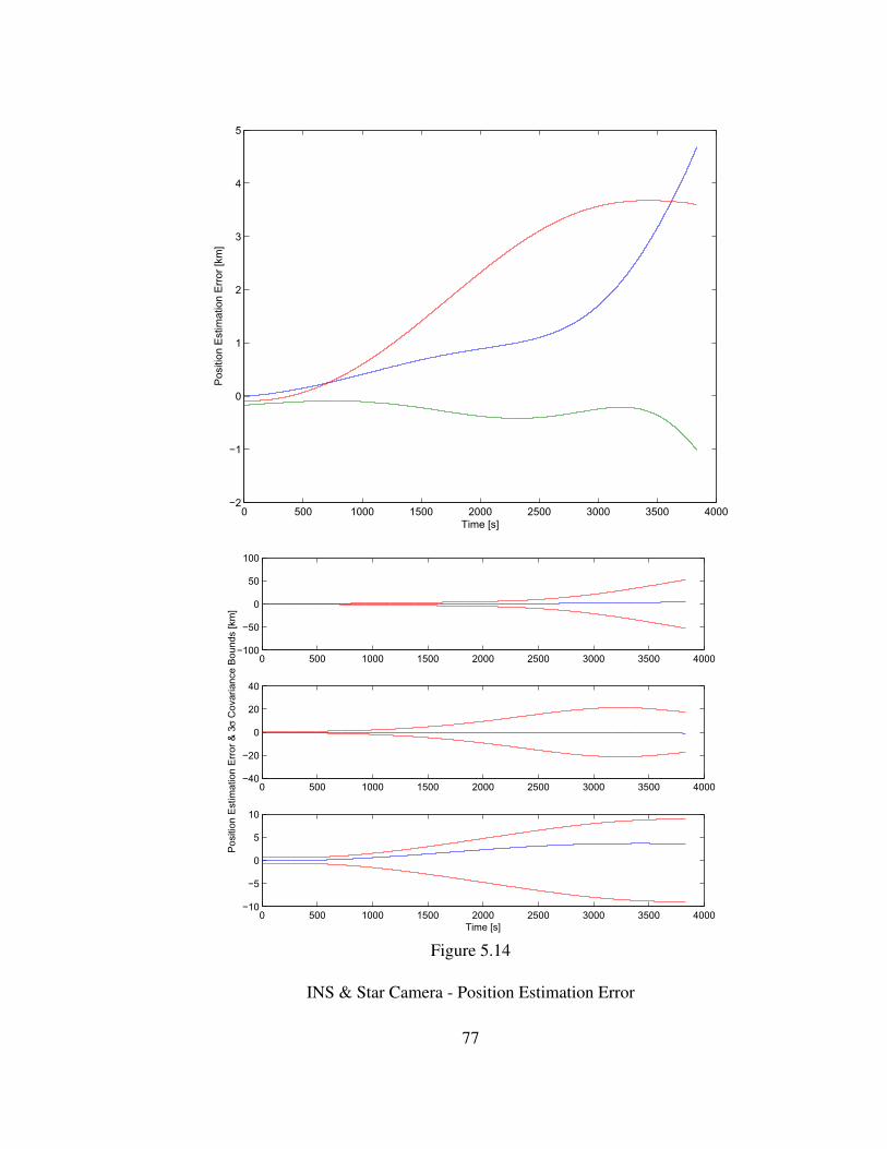
0 500 1000 1500 2000 2500 3000 3500 4000−2

−1

0

1

2

3

4

5

Time [s]

Pos

ition

Est

imat

ion

Err

or [k

m]

0 500 1000 1500 2000 2500 3000 3500 4000−100

−50

0

50

100

0 500 1000 1500 2000 2500 3000 3500 4000−40

−20

0

20

40

Pos

ition

Est

imat

ion

Err

or &

3σ

Cov

aria

nce

Bou

nds

[km

]

0 500 1000 1500 2000 2500 3000 3500 4000−10

−5

0

5

10

Time [s]

Figure 5.14

INS & Star Camera - Position Estimation Error

77

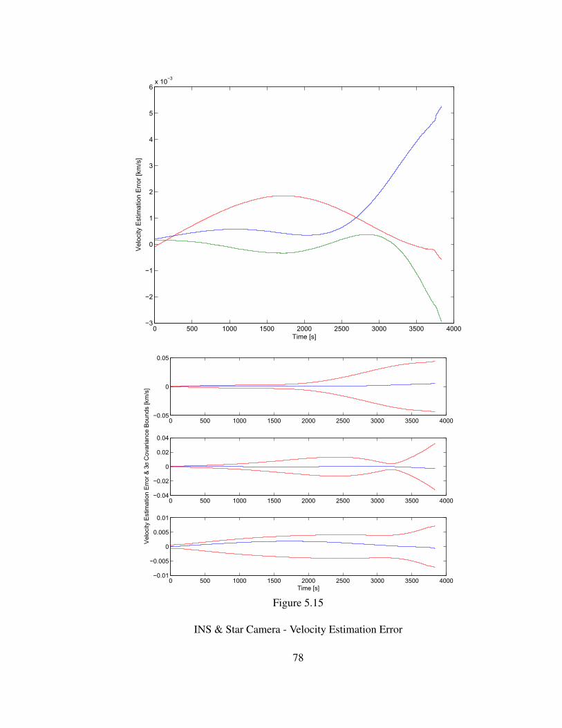
0 500 1000 1500 2000 2500 3000 3500 4000−3

−2

−1

0

1

2

3

4

5

6x 10

−3

Time [s]

Vel

ocity

Est

imat

ion

Err

or [k

m/s

]

0 500 1000 1500 2000 2500 3000 3500 4000−0.05

0

0.05

0 500 1000 1500 2000 2500 3000 3500 4000−0.04

−0.02

0

0.02

0.04

Vel

ocity

Est

imat

ion

Err

or &

3σ

Cov

aria

nce

Bou

nds

[km

/s]

0 500 1000 1500 2000 2500 3000 3500 4000−0.01

−0.005

0

0.005

0.01

Time [s]

Figure 5.15

INS & Star Camera - Velocity Estimation Error

78

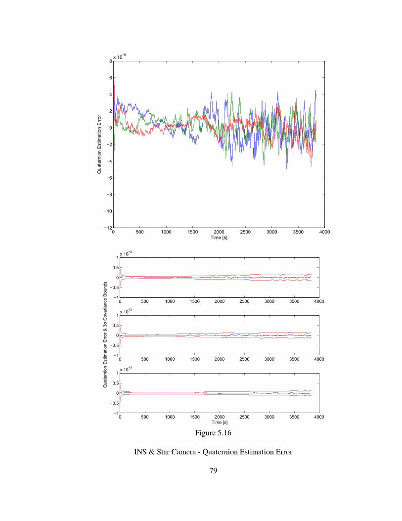
0 500 1000 1500 2000 2500 3000 3500 4000−12

−10

−8

−6

−4

−2

0

2

4

6

8x 10

−5

Time [s]

Qua

tern

ion

Est

imat

ion

Err

or

0 500 1000 1500 2000 2500 3000 3500 4000−1

−0.5

0

0.5

1x 10

−3

0 500 1000 1500 2000 2500 3000 3500 4000−1

−0.5

0

0.5

1x 10

−3

Qua

tern

ion

Est

imat

ion

Err

or &

3σ

Cov

aria

nce

Bou

nds

0 500 1000 1500 2000 2500 3000 3500 4000−1

−0.5

0

0.5

1x 10

−3

Time [s]

Figure 5.16

INS & Star Camera - Quaternion Estimation Error

79

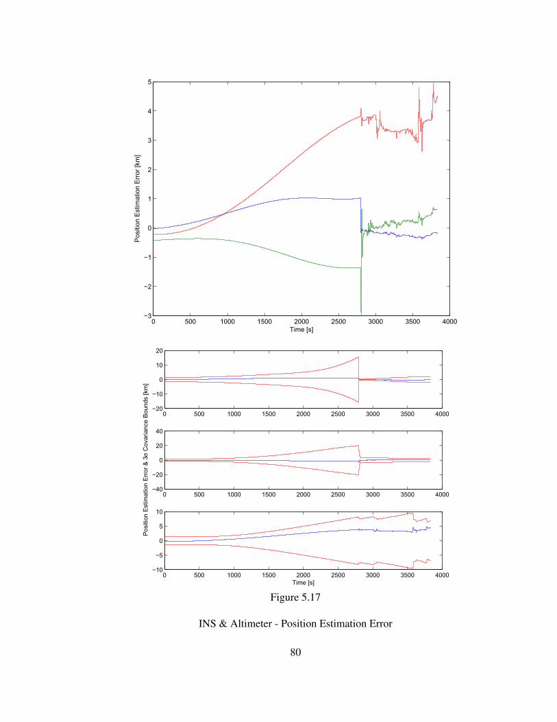
0 500 1000 1500 2000 2500 3000 3500 4000−3

−2

−1

0

1

2

3

4

5

Time [s]

Pos

ition

Est

imat

ion

Err

or [k

m]

0 500 1000 1500 2000 2500 3000 3500 4000−20

−10

0

10

20

0 500 1000 1500 2000 2500 3000 3500 4000−40

−20

0

20

40

Pos

ition

Est

imat

ion

Err

or &

3σ

Cov

aria

nce

Bou

nds

[km

]

0 500 1000 1500 2000 2500 3000 3500 4000−10

−5

0

5

10

Time [s]

Figure 5.17

INS & Altimeter - Position Estimation Error

80

0 500 1000 1500 2000 2500 3000 3500 4000−2

−1.5

−1

−0.5

0

0.5

1

1.5

2

2.5x 10

−3

Time [s]

Vel

ocity

Est

imat

ion

Err

or [k

m/s

]

0 500 1000 1500 2000 2500 3000 3500 4000−0.04

−0.02

0

0.02

0.04

0 500 1000 1500 2000 2500 3000 3500 4000−0.02

−0.01

0

0.01

0.02

Vel

ocity

Est

imat

ion

Err

or &

3σ

Cov

aria

nce

Bou

nds

[km

/s]

0 500 1000 1500 2000 2500 3000 3500 4000−0.04

−0.02

0

0.02

0.04

Time [s]

Figure 5.18

INS & Altimeter - Velocity Estimation Error

81

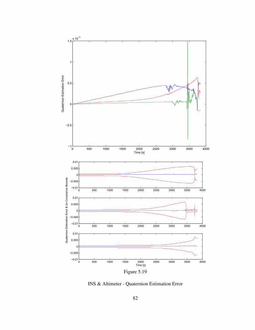
0 500 1000 1500 2000 2500 3000 3500 4000−1

−0.5

0

0.5

1

1.5x 10

−3

Time [s]

Qua

tern

ion

Est

imat

ion

Err

or

0 500 1000 1500 2000 2500 3000 3500 4000−0.01

−0.005

0

0.005

0.01

0 500 1000 1500 2000 2500 3000 3500 4000−0.01

−0.005

0

0.005

0.01

Qua

tern

ion

Est

imat

ion

Err

or &

3σ

Cov

aria

nce

Bou

nds

0 500 1000 1500 2000 2500 3000 3500 4000−0.01

−0.005

0

0.005

0.01

Time [s]

Figure 5.19

INS & Altimeter - Quaternion Estimation Error

82

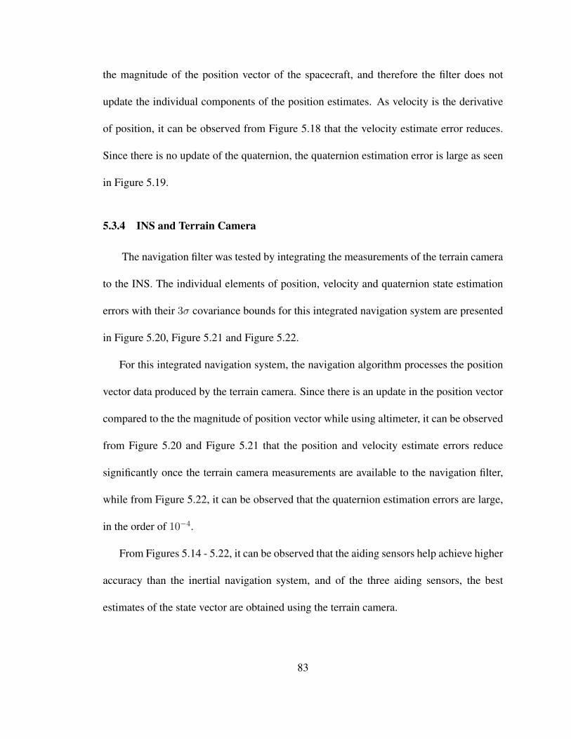
the magnitude of the position vector of the spacecraft, and therefore the filter does not

update the individual components of the position estimates. As velocity is the derivative

of position, it can be observed from Figure 5.18 that the velocity estimate error reduces.

Since there is no update of the quaternion, the quaternion estimation error is large as seen

in Figure 5.19.

5.3.4 INS and Terrain Camera

The navigation filter was tested by integrating the measurements of the terrain camera

to the INS. The individual elements of position, velocity and quaternion state estimation

errors with their 3σ covariance bounds for this integrated navigation system are presented

in Figure 5.20, Figure 5.21 and Figure 5.22.

For this integrated navigation system, the navigation algorithm processes the position

vector data produced by the terrain camera. Since there is an update in the position vector

compared to the the magnitude of position vector while using altimeter, it can be observed

from Figure 5.20 and Figure 5.21 that the position and velocity estimate errors reduce

significantly once the terrain camera measurements are available to the navigation filter,

while from Figure 5.22, it can be observed that the quaternion estimation errors are large,

in the order of 10−4.

From Figures 5.14 - 5.22, it can be observed that the aiding sensors help achieve higher

accuracy than the inertial navigation system, and of the three aiding sensors, the best

estimates of the state vector are obtained using the terrain camera.

83

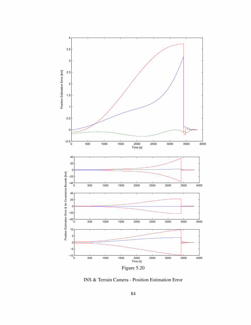
0 500 1000 1500 2000 2500 3000 3500 4000−0.5

0

0.5

1

1.5

2

2.5

3

3.5

4

Time [s]

Pos

ition

Est

imat

ion

Err

or [k

m]

0 500 1000 1500 2000 2500 3000 3500 4000−40

−20

0

20

40

0 500 1000 1500 2000 2500 3000 3500 4000−40

−20

0

20

40

Pos

ition

Est

imat

ion

Err

or &

3σ

Cov

aria

nce

Bou

nds

[km

]

0 500 1000 1500 2000 2500 3000 3500 4000−10

−5

0

5

10

Time [s]

Figure 5.20

INS & Terrain Camera - Position Estimation Error

84

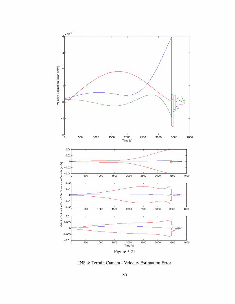
0 500 1000 1500 2000 2500 3000 3500 4000−2

−1

0

1

2

3

4x 10

−3

Time [s]

Vel

ocity

Est

imat

ion

Err

or [k

m/s

]

0 500 1000 1500 2000 2500 3000 3500 4000−0.04

−0.02

0

0.02

0.04

0 500 1000 1500 2000 2500 3000 3500 4000−0.02

−0.01

0

0.01

0.02

Vel

ocity

Est

imat

ion

Err

or &

3σ

Cov

aria

nce

Bou

nds

[km

/s]

0 500 1000 1500 2000 2500 3000 3500 4000−0.01

−0.005

0

0.005

0.01

Time [s]

Figure 5.21

INS & Terrain Camera - Velocity Estimation Error

85

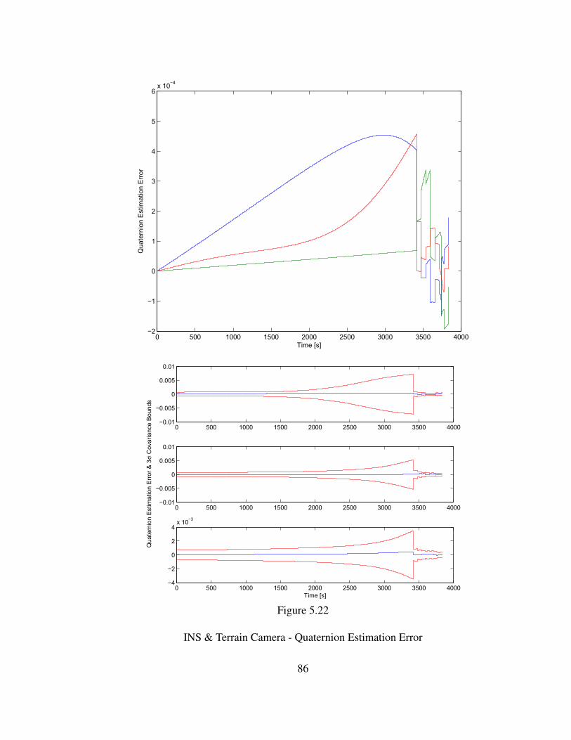
0 500 1000 1500 2000 2500 3000 3500 4000−2

−1

0

1

2

3

4

5

6x 10

−4

Time [s]

Qua

tern

ion

Est

imat

ion

Err

or

0 500 1000 1500 2000 2500 3000 3500 4000−0.01

−0.005

0

0.005

0.01

0 500 1000 1500 2000 2500 3000 3500 4000−0.01

−0.005

0

0.005

0.01

Qua

tern

ion

Est

imat

ion

Err

or &

3σ

Cov

aria

nce

Bou

nds

0 500 1000 1500 2000 2500 3000 3500 4000−4

−2

0

2

4x 10

−3

Time [s]

Figure 5.22

INS & Terrain Camera - Quaternion Estimation Error

86

5.3.5 INS, Star Camera and Altimeter

The navigation filter was tested by integrating the measurements of the star camera

and altimeter to the INS. The individual elements of position, velocity and quaternion state

estimation errors with their 3σ covariance bounds for this integrated navigation system are

presented in Figure 5.23, Figure 5.24 and Figure 5.25.

For this navigation system, the navigation algorithm processes the quaternion measure-

ments from the star camera and the altitude (position) measurements from the altimeter.

Since there is an update in both magnitude of the position vector and the quaternion, from

Figure 5.23 and Figure 5.24, it can be observed that the position and velocity estimation

errors reduce compared to the previous observations, and from Figure 5.25, the quaternion

estimation errors reduce significantly to the order of 10−5.

5.3.6 INS, Star Camera and Terrain Camera

The navigation filter was tested by integrating the measurements of the star camera

and the terrain camera to the INS. The individual elements of state estimation errors with

their 3σ covariance bounds for this integrated navigation system are presented in Figure

5.26, Figure 5.27 and Figure 5.28.

For this integrated navigation system, the navigation filter processes the position vector

measurements from the terrain camera and quaternion measurements from the star camera.

From Figure 5.26 and Figure 5.27, it can be observed that the terrain camera produces bet-

ter estimates of the position and velocity vectors, while from Figure 5.28, the star camera

quaternion measurements help improve the quaternion error estimates significantly.

87

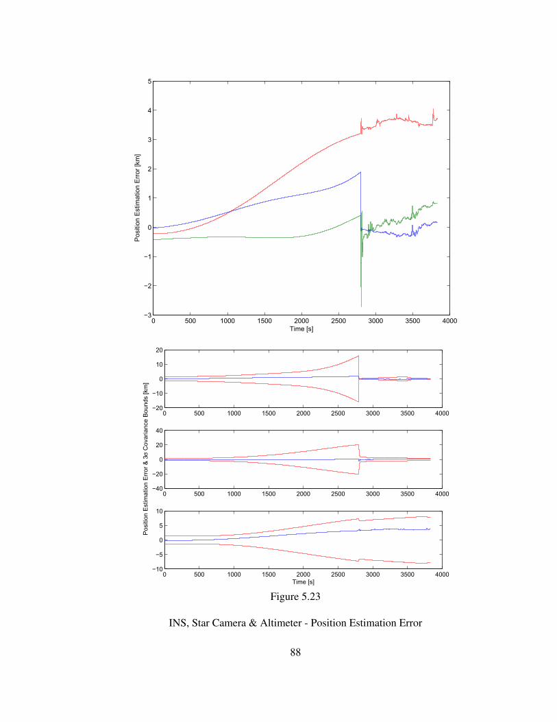
0 500 1000 1500 2000 2500 3000 3500 4000−3

−2

−1

0

1

2

3

4

5

Time [s]

Pos

ition

Est

imat

ion

Err

or [k

m]

0 500 1000 1500 2000 2500 3000 3500 4000−20

−10

0

10

20

0 500 1000 1500 2000 2500 3000 3500 4000−40

−20

0

20

40

Pos

ition

Est

imat

ion

Err

or &

3σ

Cov

aria

nce

Bou

nds

[km

]

0 500 1000 1500 2000 2500 3000 3500 4000−10

−5

0

5

10

Time [s]

Figure 5.23

INS, Star Camera & Altimeter - Position Estimation Error

88

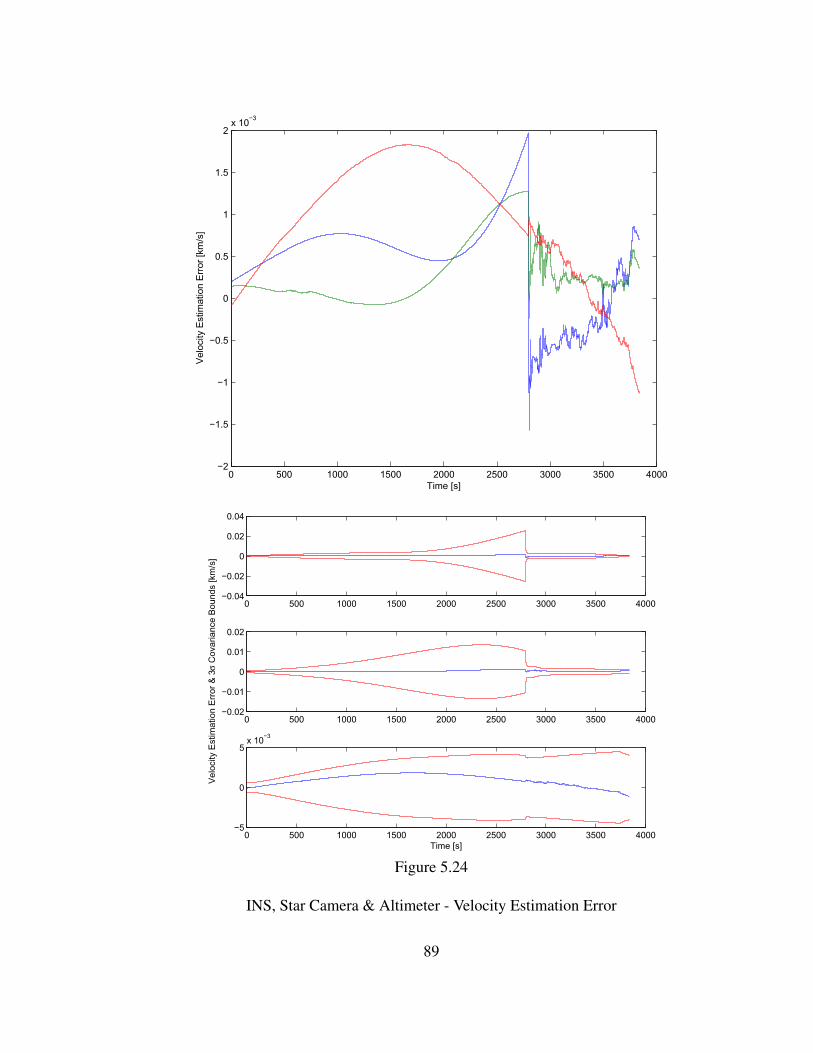
0 500 1000 1500 2000 2500 3000 3500 4000−2

−1.5

−1

−0.5

0

0.5

1

1.5

2x 10

−3

Time [s]

Vel

ocity

Est

imat

ion

Err

or [k

m/s

]

0 500 1000 1500 2000 2500 3000 3500 4000−0.04

−0.02

0

0.02

0.04

0 500 1000 1500 2000 2500 3000 3500 4000−0.02

−0.01

0

0.01

0.02

Vel

ocity

Est

imat

ion

Err

or &

3σ

Cov

aria

nce

Bou

nds

[km

/s]

0 500 1000 1500 2000 2500 3000 3500 4000−5

0

5x 10

−3

Time [s]

Figure 5.24

INS, Star Camera & Altimeter - Velocity Estimation Error

89

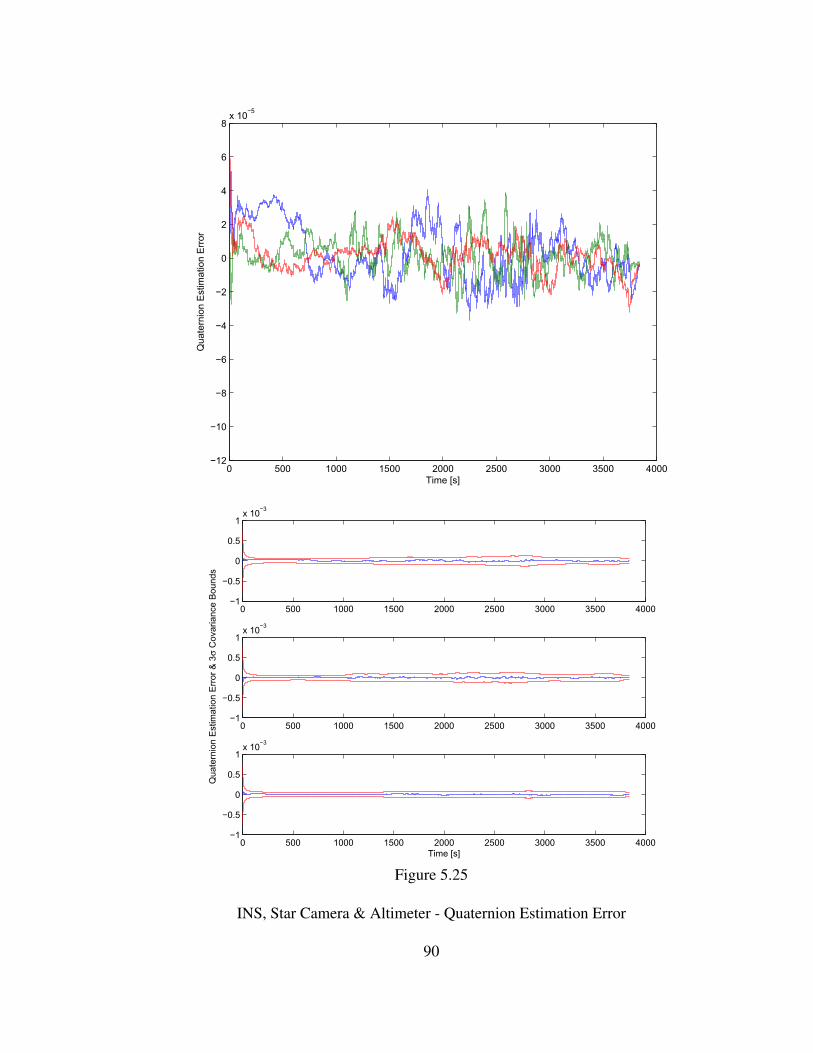
0 500 1000 1500 2000 2500 3000 3500 4000−12

−10

−8

−6

−4

−2

0

2

4

6

8x 10

−5

Time [s]

Qua

tern

ion

Est

imat

ion

Err

or

0 500 1000 1500 2000 2500 3000 3500 4000−1

−0.5

0

0.5

1x 10

−3

0 500 1000 1500 2000 2500 3000 3500 4000−1

−0.5

0

0.5

1x 10

−3

Qua

tern

ion

Est

imat

ion

Err

or &

3σ

Cov

aria

nce

Bou

nds

0 500 1000 1500 2000 2500 3000 3500 4000−1

−0.5

0

0.5

1x 10

−3

Time [s]

Figure 5.25

INS, Star Camera & Altimeter - Quaternion Estimation Error

90

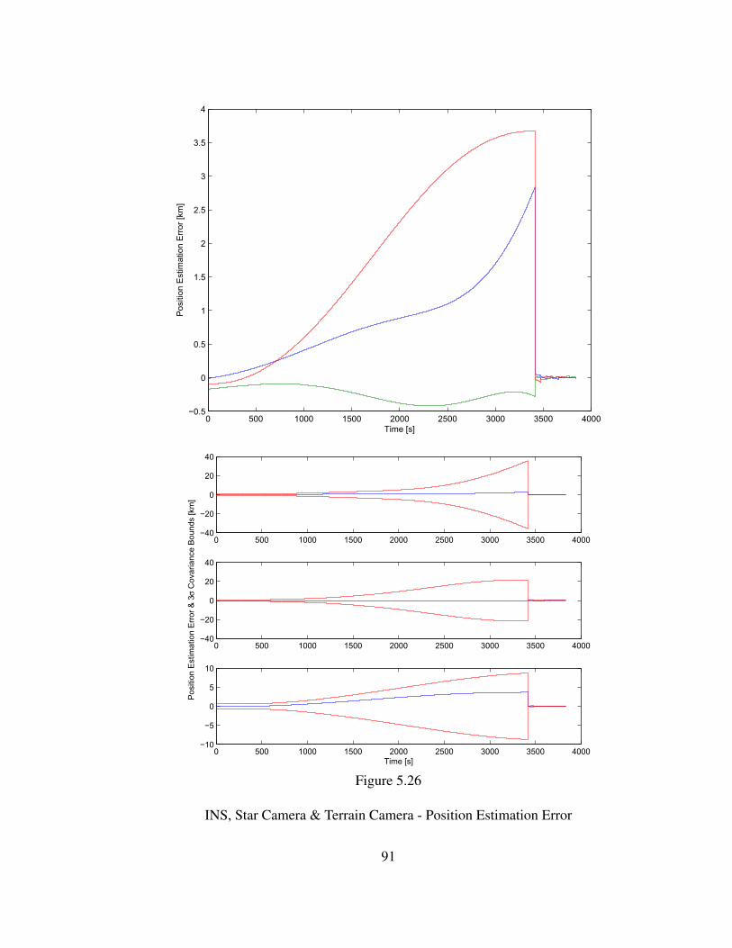
0 500 1000 1500 2000 2500 3000 3500 4000−0.5

0

0.5

1

1.5

2

2.5

3

3.5

4

Time [s]

Pos

ition

Est

imat

ion

Err

or [k

m]

0 500 1000 1500 2000 2500 3000 3500 4000−40

−20

0

20

40

0 500 1000 1500 2000 2500 3000 3500 4000−40

−20

0

20

40

Pos

ition

Est

imat

ion

Err

or &

3σ

Cov

aria

nce

Bou

nds

[km

]

0 500 1000 1500 2000 2500 3000 3500 4000−10

−5

0

5

10

Time [s]

Figure 5.26

INS, Star Camera & Terrain Camera - Position Estimation Error

91

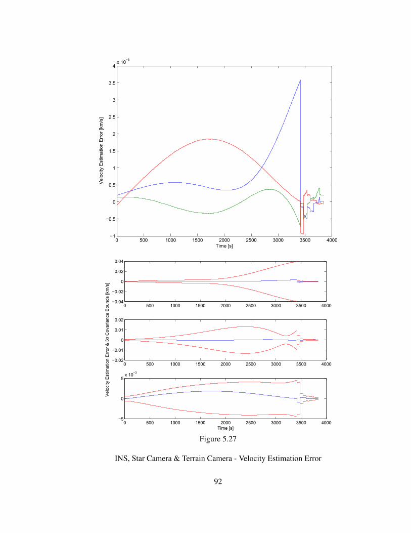
0 500 1000 1500 2000 2500 3000 3500 4000−1

−0.5

0

0.5

1

1.5

2

2.5

3

3.5

4x 10

−3

Time [s]

Vel

ocity

Est

imat

ion

Err

or [k

m/s

]

0 500 1000 1500 2000 2500 3000 3500 4000−0.04

−0.02

0

0.02

0.04

0 500 1000 1500 2000 2500 3000 3500 4000−0.02

−0.01

0

0.01

0.02

Vel

ocity

Est

imat

ion

Err

or &

3σ

Cov

aria

nce

Bou

nds

[km

/s]

0 500 1000 1500 2000 2500 3000 3500 4000−5

0

5x 10

−3

Time [s]

Figure 5.27

INS, Star Camera & Terrain Camera - Velocity Estimation Error

92

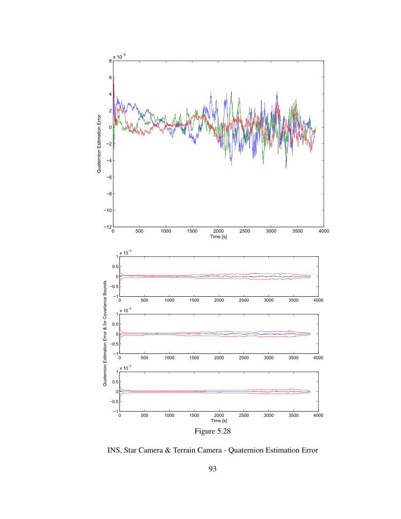
0 500 1000 1500 2000 2500 3000 3500 4000−12

−10

−8

−6

−4

−2

0

2

4

6

8x 10

−5

Time [s]

Qua

tern

ion

Est

imat

ion

Err

or

0 500 1000 1500 2000 2500 3000 3500 4000−1

−0.5

0

0.5

1x 10

−3

0 500 1000 1500 2000 2500 3000 3500 4000−1

−0.5

0

0.5

1x 10

−3

Qua

tern

ion

Est

imat

ion

Err

or &

3σ

Cov

aria

nce

Bou

nds

0 500 1000 1500 2000 2500 3000 3500 4000−1

−0.5

0

0.5

1x 10

−3

Time [s]

Figure 5.28

INS, Star Camera & Terrain Camera - Quaternion Estimation Error

93

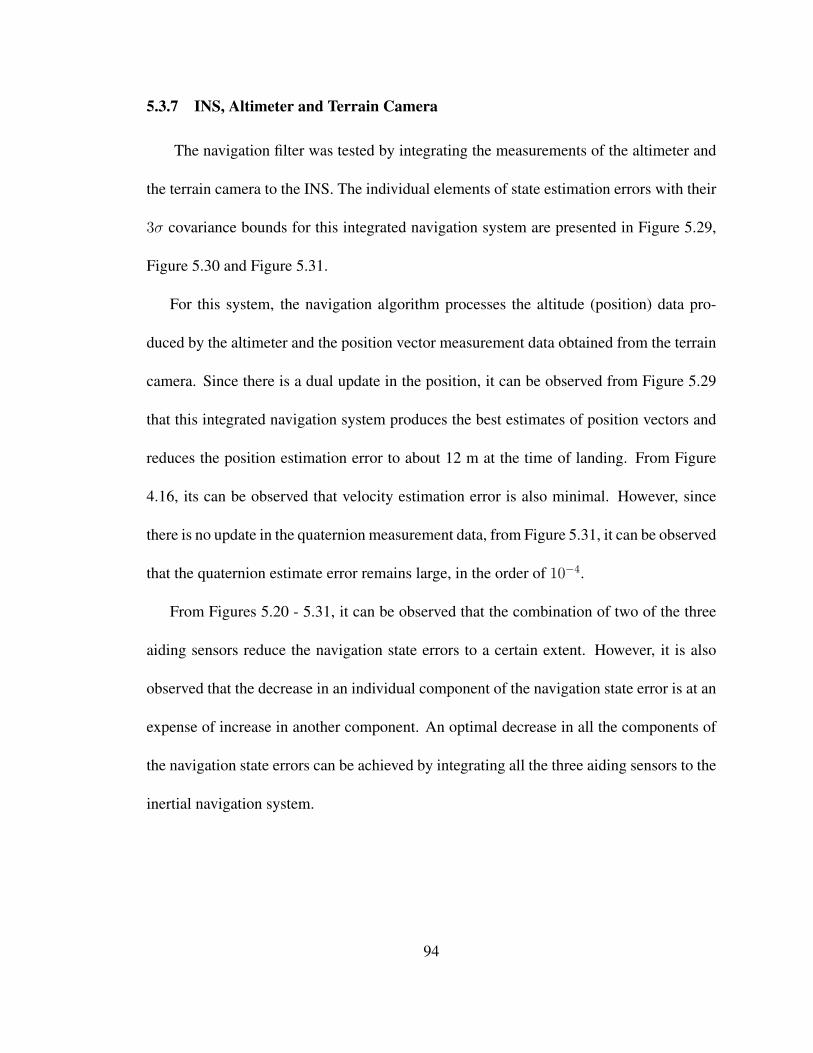
5.3.7 INS, Altimeter and Terrain Camera

The navigation filter was tested by integrating the measurements of the altimeter and

the terrain camera to the INS. The individual elements of state estimation errors with their

3σ covariance bounds for this integrated navigation system are presented in Figure 5.29,

Figure 5.30 and Figure 5.31.

For this system, the navigation algorithm processes the altitude (position) data pro-

duced by the altimeter and the position vector measurement data obtained from the terrain

camera. Since there is a dual update in the position, it can be observed from Figure 5.29

that this integrated navigation system produces the best estimates of position vectors and

reduces the position estimation error to about 12 m at the time of landing. From Figure

4.16, its can be observed that velocity estimation error is also minimal. However, since

there is no update in the quaternion measurement data, from Figure 5.31, it can be observed

that the quaternion estimate error remains large, in the order of 10−4.

From Figures 5.20 - 5.31, it can be observed that the combination of two of the three

aiding sensors reduce the navigation state errors to a certain extent. However, it is also

observed that the decrease in an individual component of the navigation state error is at an

expense of increase in another component. An optimal decrease in all the components of

the navigation state errors can be achieved by integrating all the three aiding sensors to the

inertial navigation system.

94

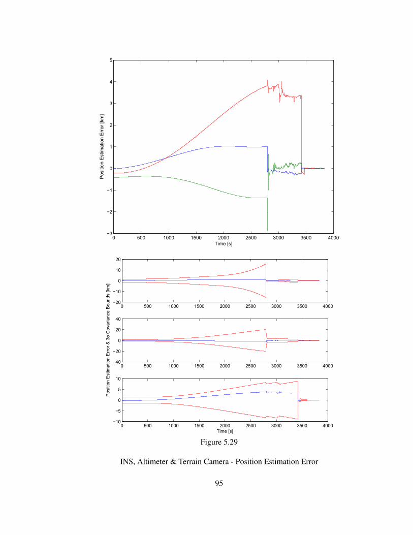
0 500 1000 1500 2000 2500 3000 3500 4000−3

−2

−1

0

1

2

3

4

5

Time [s]

Pos

ition

Est

imat

ion

Err

or [k

m]

0 500 1000 1500 2000 2500 3000 3500 4000−20

−10

0

10

20

0 500 1000 1500 2000 2500 3000 3500 4000−40

−20

0

20

40

Pos

ition

Est

imat

ion

Err

or &

3σ

Cov

aria

nce

Bou

nds

[km

]

0 500 1000 1500 2000 2500 3000 3500 4000−10

−5

0

5

10

Time [s]

Figure 5.29

INS, Altimeter & Terrain Camera - Position Estimation Error

95

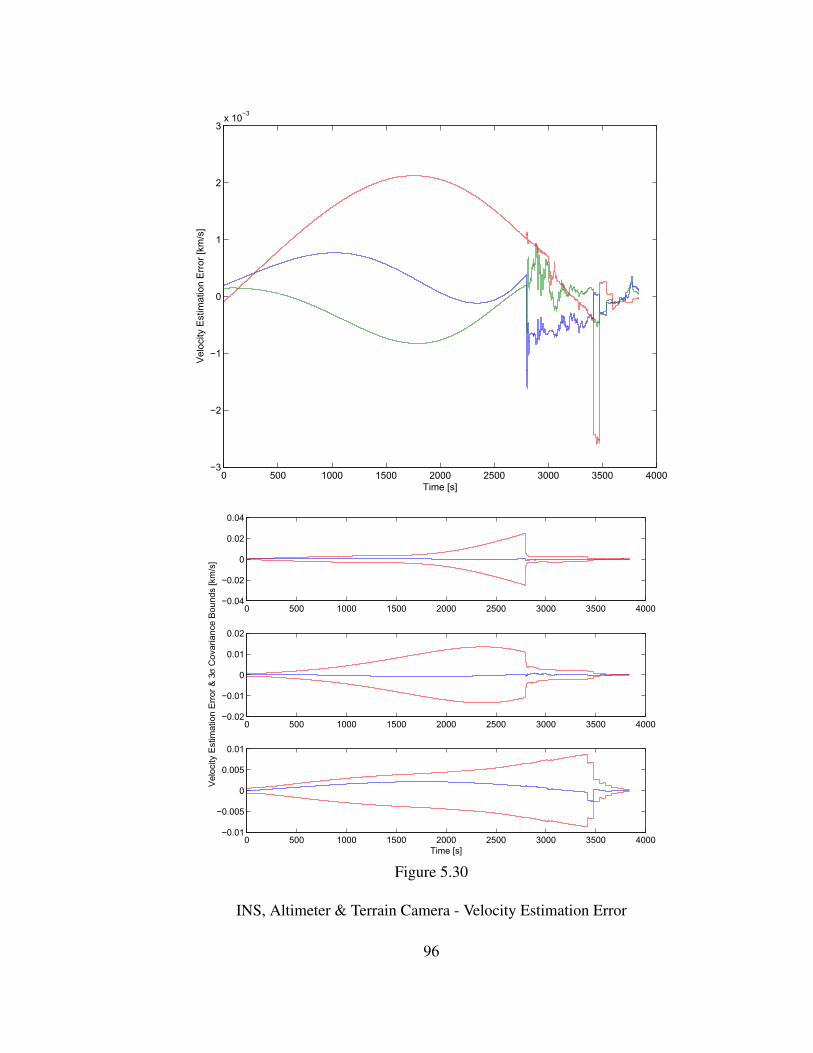
0 500 1000 1500 2000 2500 3000 3500 4000−3

−2

−1

0

1

2

3x 10

−3

Time [s]

Vel

ocity

Est

imat

ion

Err

or [k

m/s

]

0 500 1000 1500 2000 2500 3000 3500 4000−0.04

−0.02

0

0.02

0.04

0 500 1000 1500 2000 2500 3000 3500 4000−0.02

−0.01

0

0.01

0.02

Vel

ocity

Est

imat

ion

Err

or &

3σ

Cov

aria

nce

Bou

nds

[km

/s]

0 500 1000 1500 2000 2500 3000 3500 4000−0.01

−0.005

0

0.005

0.01

Time [s]

Figure 5.30

INS, Altimeter & Terrain Camera - Velocity Estimation Error

96

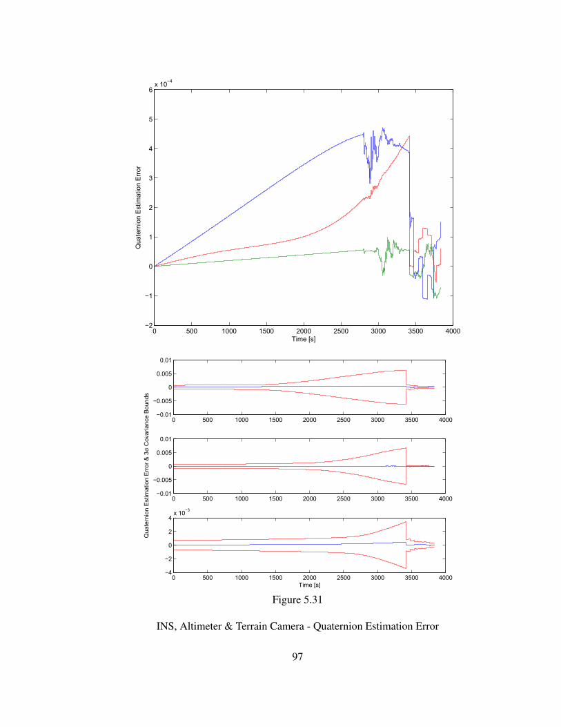
0 500 1000 1500 2000 2500 3000 3500 4000−2

−1

0

1

2

3

4

5

6x 10

−4

Time [s]

Qua

tern

ion

Est

imat

ion

Err

or

0 500 1000 1500 2000 2500 3000 3500 4000−0.01

−0.005

0

0.005

0.01

0 500 1000 1500 2000 2500 3000 3500 4000−0.01

−0.005

0

0.005

0.01

Qua

tern

ion

Est

imat

ion

Err

or &

3σ

Cov

aria

nce

Bou

nds

0 500 1000 1500 2000 2500 3000 3500 4000−4

−2

0

2

4x 10

−3

Time [s]

Figure 5.31

INS, Altimeter & Terrain Camera - Quaternion Estimation Error

97

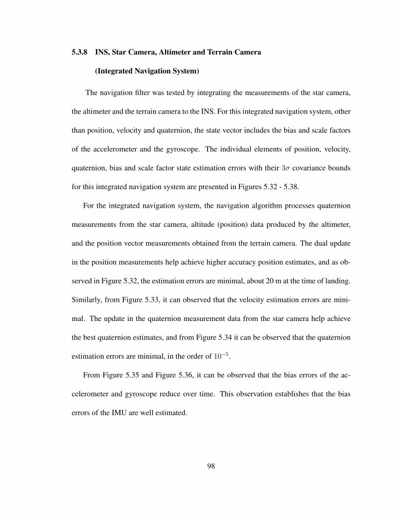
5.3.8 INS, Star Camera, Altimeter and Terrain Camera

(Integrated Navigation System)

The navigation filter was tested by integrating the measurements of the star camera,

the altimeter and the terrain camera to the INS. For this integrated navigation system, other

than position, velocity and quaternion, the state vector includes the bias and scale factors

of the accelerometer and the gyroscope. The individual elements of position, velocity,

quaternion, bias and scale factor state estimation errors with their 3σ covariance bounds

for this integrated navigation system are presented in Figures 5.32 - 5.38.

For the integrated navigation system, the navigation algorithm processes quaternion

measurements from the star camera, altitude (position) data produced by the altimeter,

and the position vector measurements obtained from the terrain camera. The dual update

in the position measurements help achieve higher accuracy position estimates, and as ob-

served in Figure 5.32, the estimation errors are minimal, about 20 m at the time of landing.

Similarly, from Figure 5.33, it can observed that the velocity estimation errors are mini-

mal. The update in the quaternion measurement data from the star camera help achieve

the best quaternion estimates, and from Figure 5.34 it can be observed that the quaternion

estimation errors are minimal, in the order of 10−5.

From Figure 5.35 and Figure 5.36, it can be observed that the bias errors of the ac-

celerometer and gyroscope reduce over time. This observation establishes that the bias

errors of the IMU are well estimated.

98

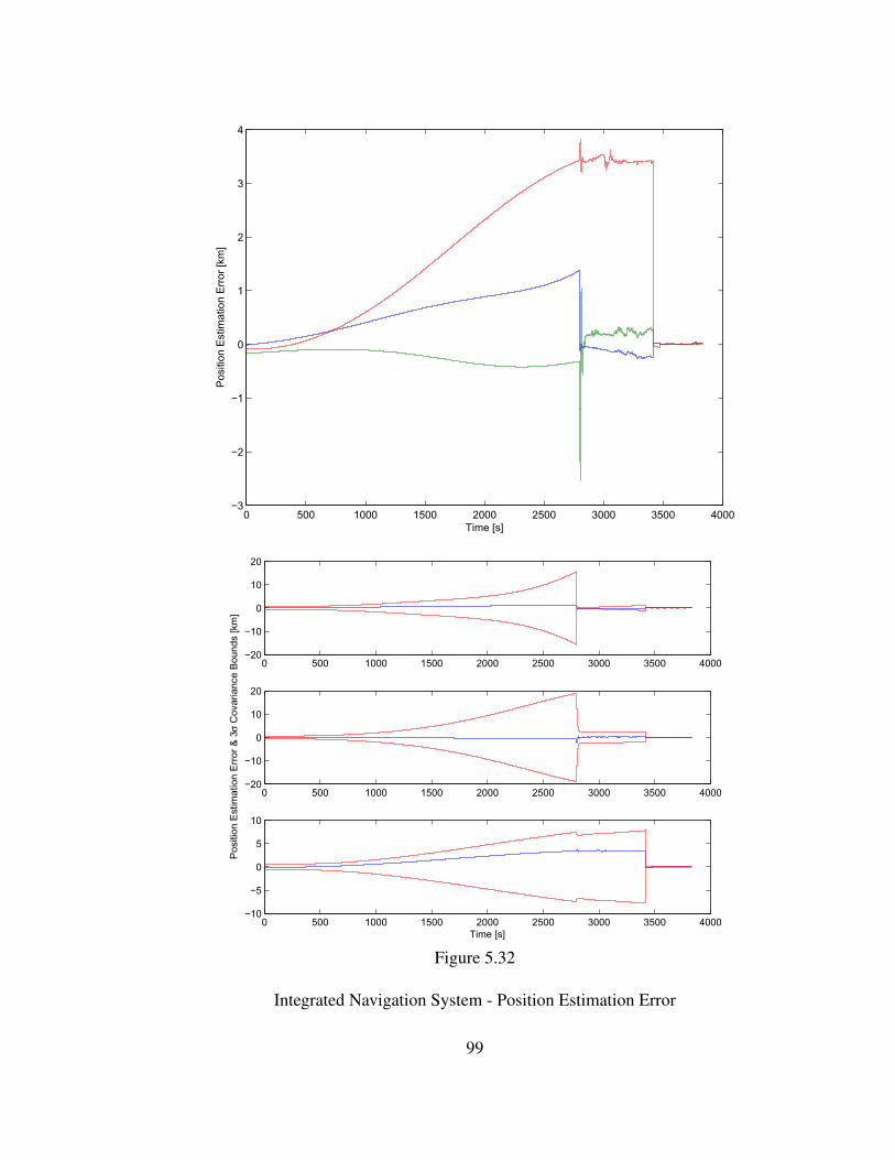
0 500 1000 1500 2000 2500 3000 3500 4000−3

−2

−1

0

1

2

3

4

Time [s]

Pos

ition

Est

imat

ion

Err

or [k

m]

0 500 1000 1500 2000 2500 3000 3500 4000−20

−10

0

10

20

0 500 1000 1500 2000 2500 3000 3500 4000−20

−10

0

10

20

Pos

ition

Est

imat

ion

Err

or &

3σ

Cov

aria

nce

Bou

nds

[km

]

0 500 1000 1500 2000 2500 3000 3500 4000−10

−5

0

5

10

Time [s]

Figure 5.32

Integrated Navigation System - Position Estimation Error

99

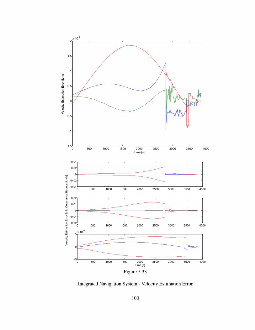
0 500 1000 1500 2000 2500 3000 3500 4000−1.5

−1

−0.5

0

0.5

1

1.5

2x 10

−3

Time [s]

Vel

ocity

Est

imat

ion

Err

or [k

m/s

]

0 500 1000 1500 2000 2500 3000 3500 4000−0.04

−0.02

0

0.02

0.04

0 500 1000 1500 2000 2500 3000 3500 4000−0.02

−0.01

0

0.01

0.02

Vel

ocity

Est

imat

ion

Err

or &

3σ

Cov

aria

nce

Bou

nds

[km

/s]

0 500 1000 1500 2000 2500 3000 3500 4000−5

0

5x 10

−3

Time [s]

Figure 5.33

Integrated Navigation System - Velocity Estimation Error

100

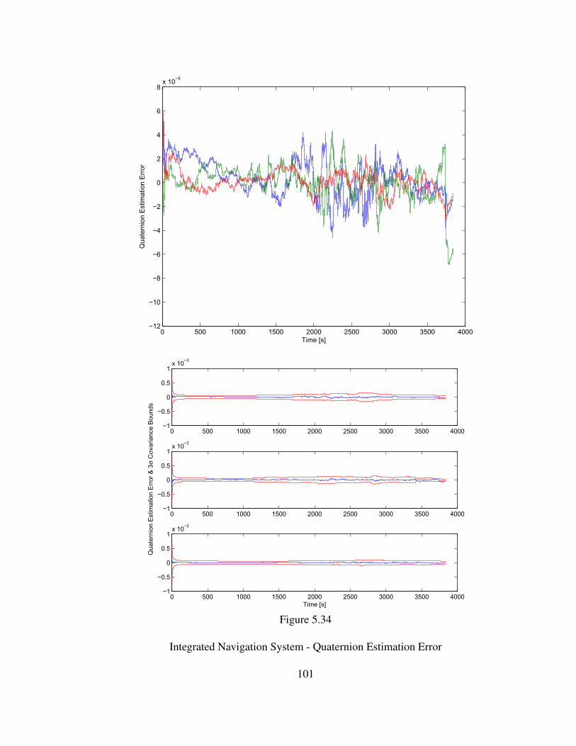
0 500 1000 1500 2000 2500 3000 3500 4000−12

−10

−8

−6

−4

−2

0

2

4

6

8x 10

−5

Time [s]

Qua

tern

ion

Est

imat

ion

Err

or

0 500 1000 1500 2000 2500 3000 3500 4000−1

−0.5

0

0.5

1x 10

−3

0 500 1000 1500 2000 2500 3000 3500 4000−1

−0.5

0

0.5

1x 10

−3

Qua

tern

ion

Est

imat

ion

Err

or &

3σ

Cov

aria

nce

Bou

nds

0 500 1000 1500 2000 2500 3000 3500 4000−1

−0.5

0

0.5

1x 10

−3

Time [s]

Figure 5.34

Integrated Navigation System - Quaternion Estimation Error

101

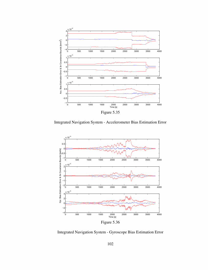
0 500 1000 1500 2000 2500 3000 3500 4000−4

−2

0

2

4x 10

−6

0 500 1000 1500 2000 2500 3000 3500 4000−1

−0.5

0

0.5

1x 10

−5

Acc

. Bia

s E

stim

atio

n E

rror

& 3

σ C

ovar

ianc

e B

ound

s [k

m/s

2 ]

0 500 1000 1500 2000 2500 3000 3500 4000−1

−0.5

0

0.5

1x 10

−5

Time [s]

Figure 5.35

Integrated Navigation System - Accelerometer Bias Estimation Error

0 500 1000 1500 2000 2500 3000 3500 4000−1

−0.5

0

0.5

1x 10

−5

0 500 1000 1500 2000 2500 3000 3500 4000−2

−1

0

1

2x 10

−5

Gyr

. Bia

s E

stim

atio

n E

rror

& 3

σ C

ovar

ianc

e B

ound

s [r

ad/s

]

0 500 1000 1500 2000 2500 3000 3500 4000−4

−2

0

2

4x 10

−6

Time [s]

Figure 5.36

Integrated Navigation System - Gyroscope Bias Estimation Error

102

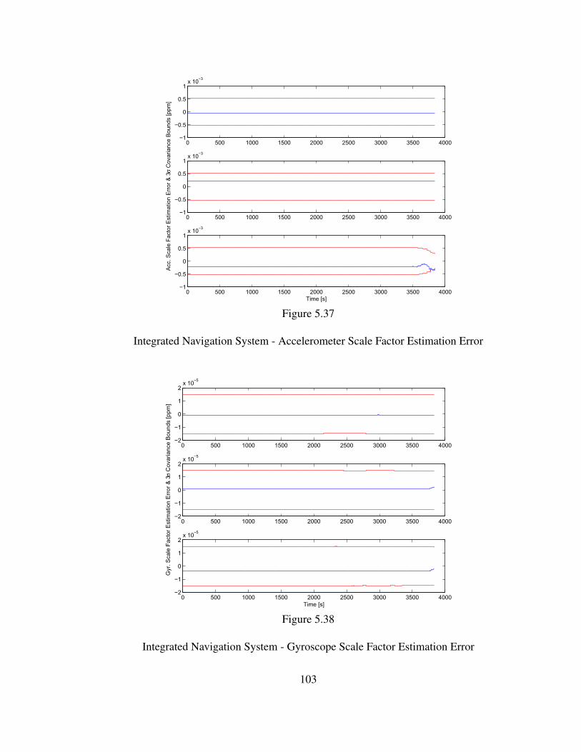
0 500 1000 1500 2000 2500 3000 3500 4000−1

−0.5

0

0.5

1x 10

−3

0 500 1000 1500 2000 2500 3000 3500 4000−1

−0.5

0

0.5

1x 10

−3

Acc

. Sca

le F

acto

r E

stim

atio

n E

rror

& 3

σ C

ovar

ianc

e B

ound

s [p

pm]

0 500 1000 1500 2000 2500 3000 3500 4000−1

−0.5

0

0.5

1x 10

−3

Time [s]

Figure 5.37

Integrated Navigation System - Accelerometer Scale Factor Estimation Error

0 500 1000 1500 2000 2500 3000 3500 4000−2

−1

0

1

2x 10

−5

0 500 1000 1500 2000 2500 3000 3500 4000−2

−1

0

1

2x 10

−5

Gyr

. Sca

le F

acto

r E

stim

atio

n E

rror

& 3

σ C

ovar

ianc

e B

ound

s [p

pm]

0 500 1000 1500 2000 2500 3000 3500 4000−2

−1

0

1

2x 10

−5

Time [s]

Figure 5.38

Integrated Navigation System - Gyroscope Scale Factor Estimation Error

103

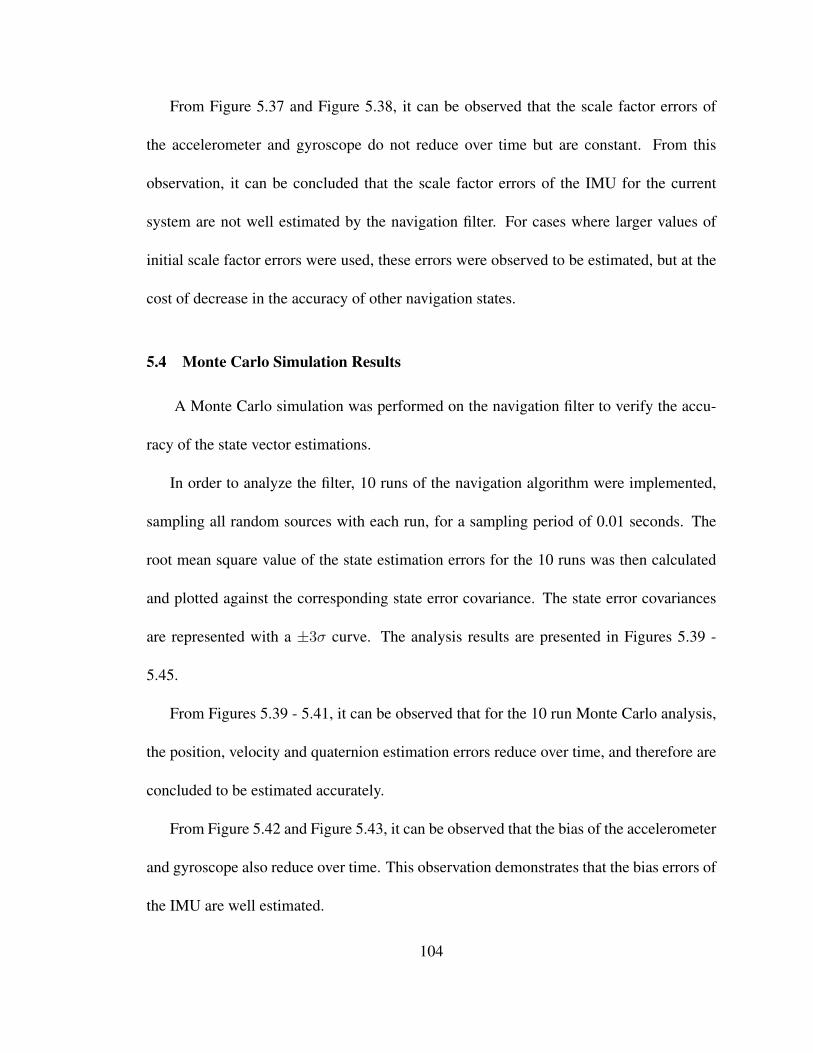
From Figure 5.37 and Figure 5.38, it can be observed that the scale factor errors of

the accelerometer and gyroscope do not reduce over time but are constant. From this

observation, it can be concluded that the scale factor errors of the IMU for the current

system are not well estimated by the navigation filter. For cases where larger values of

initial scale factor errors were used, these errors were observed to be estimated, but at the

cost of decrease in the accuracy of other navigation states.

5.4 Monte Carlo Simulation Results

A Monte Carlo simulation was performed on the navigation filter to verify the accu-

racy of the state vector estimations.

In order to analyze the filter, 10 runs of the navigation algorithm were implemented,

sampling all random sources with each run, for a sampling period of 0.01 seconds. The

root mean square value of the state estimation errors for the 10 runs was then calculated

and plotted against the corresponding state error covariance. The state error covariances

are represented with a ±3σ curve. The analysis results are presented in Figures 5.39 -

5.45.

From Figures 5.39 - 5.41, it can be observed that for the 10 run Monte Carlo analysis,

the position, velocity and quaternion estimation errors reduce over time, and therefore are

concluded to be estimated accurately.

From Figure 5.42 and Figure 5.43, it can be observed that the bias of the accelerometer

and gyroscope also reduce over time. This observation demonstrates that the bias errors of

the IMU are well estimated.

104

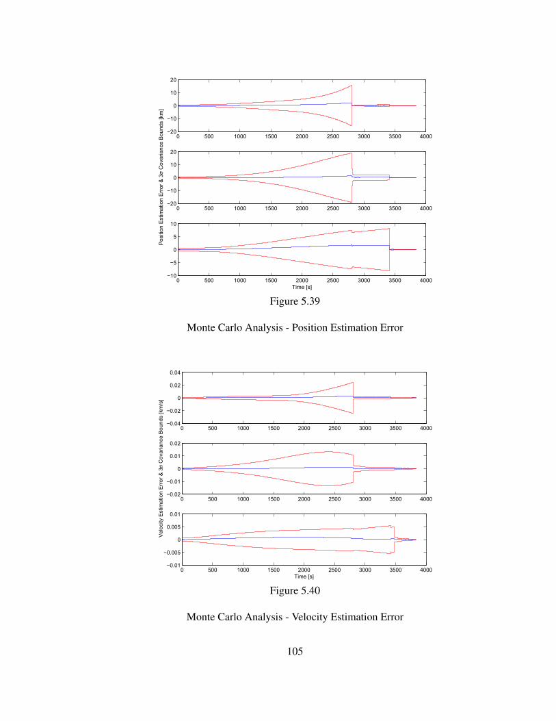
0 500 1000 1500 2000 2500 3000 3500 4000−20

−10

0

10

20

0 500 1000 1500 2000 2500 3000 3500 4000−20

−10

0

10

20

Pos

ition

Est

imat

ion

Err

or &

3σ

Cov

aria

nce

Bou

nds

[km

]

0 500 1000 1500 2000 2500 3000 3500 4000−10

−5

0

5

10

Time [s]

Figure 5.39

Monte Carlo Analysis - Position Estimation Error

0 500 1000 1500 2000 2500 3000 3500 4000−0.04

−0.02

0

0.02

0.04

0 500 1000 1500 2000 2500 3000 3500 4000−0.02

−0.01

0

0.01

0.02

Vel

ocity

Est

imat

ion

Err

or &

3σ

Cov

aria

nce

Bou

nds

[km

/s]

0 500 1000 1500 2000 2500 3000 3500 4000−0.01

−0.005

0

0.005

0.01

Time [s]

Figure 5.40

Monte Carlo Analysis - Velocity Estimation Error

105

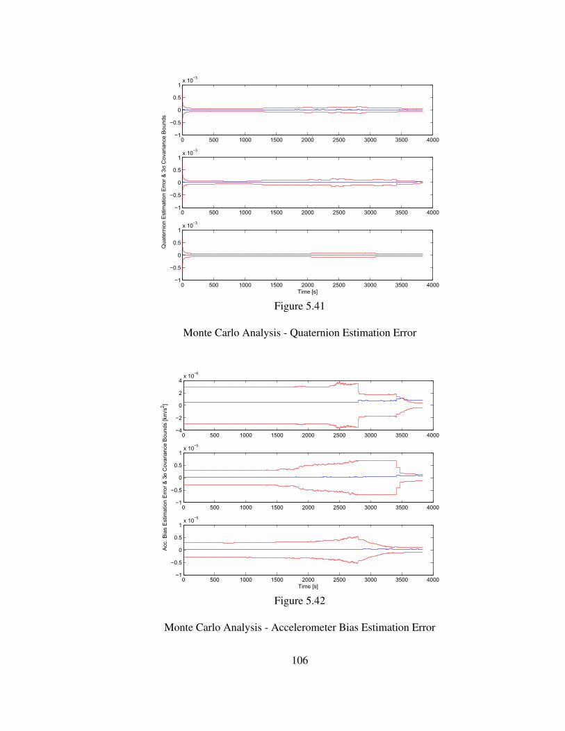
0 500 1000 1500 2000 2500 3000 3500 4000−1

−0.5

0

0.5

1x 10

−3

0 500 1000 1500 2000 2500 3000 3500 4000−1

−0.5

0

0.5

1x 10

−3

Qua

tern

ion

Est

imat

ion

Err

or &

3σ

Cov

aria

nce

Bou

nds

0 500 1000 1500 2000 2500 3000 3500 4000−1

−0.5

0

0.5

1x 10

−3

Time [s]

Figure 5.41

Monte Carlo Analysis - Quaternion Estimation Error

0 500 1000 1500 2000 2500 3000 3500 4000−4

−2

0

2

4x 10

−6

0 500 1000 1500 2000 2500 3000 3500 4000−1

−0.5

0

0.5

1x 10

−5

Acc

. Bia

s E

stim

atio

n E

rror

& 3

σ C

ovar

ianc

e B

ound

s [k

m/s

2 ]

0 500 1000 1500 2000 2500 3000 3500 4000−1

−0.5

0

0.5

1x 10

−5

Time [s]

Figure 5.42

Monte Carlo Analysis - Accelerometer Bias Estimation Error

106

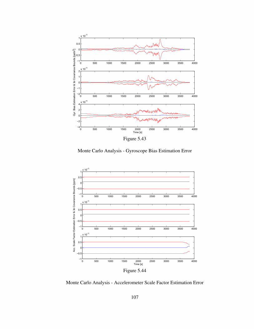
0 500 1000 1500 2000 2500 3000 3500 4000−1

−0.5

0

0.5

1x 10

−5

0 500 1000 1500 2000 2500 3000 3500 4000−2

−1

0

1

2x 10

−5

Gyr

. Bia

s E

stim

atio

n E

rror

& 3

σ C

ovar

ianc

e B

ound

s [r

ad/s

2 ]

0 500 1000 1500 2000 2500 3000 3500 4000−4

−2

0

2

4x 10

−6

Time [s]

Figure 5.43

Monte Carlo Analysis - Gyroscope Bias Estimation Error

0 500 1000 1500 2000 2500 3000 3500 4000−1

−0.5

0

0.5

1x 10

−3

0 500 1000 1500 2000 2500 3000 3500 4000−1

−0.5

0

0.5

1x 10

−3

Acc

. Sca

le F

acto

r E

stim

atio

n E

rror

& 3

σ C

ovar

ianc

e B

ound

s [p

pm]

0 500 1000 1500 2000 2500 3000 3500 4000−1

−0.5

0

0.5

1x 10

−3

Time [s]

Figure 5.44

Monte Carlo Analysis - Accelerometer Scale Factor Estimation Error

107

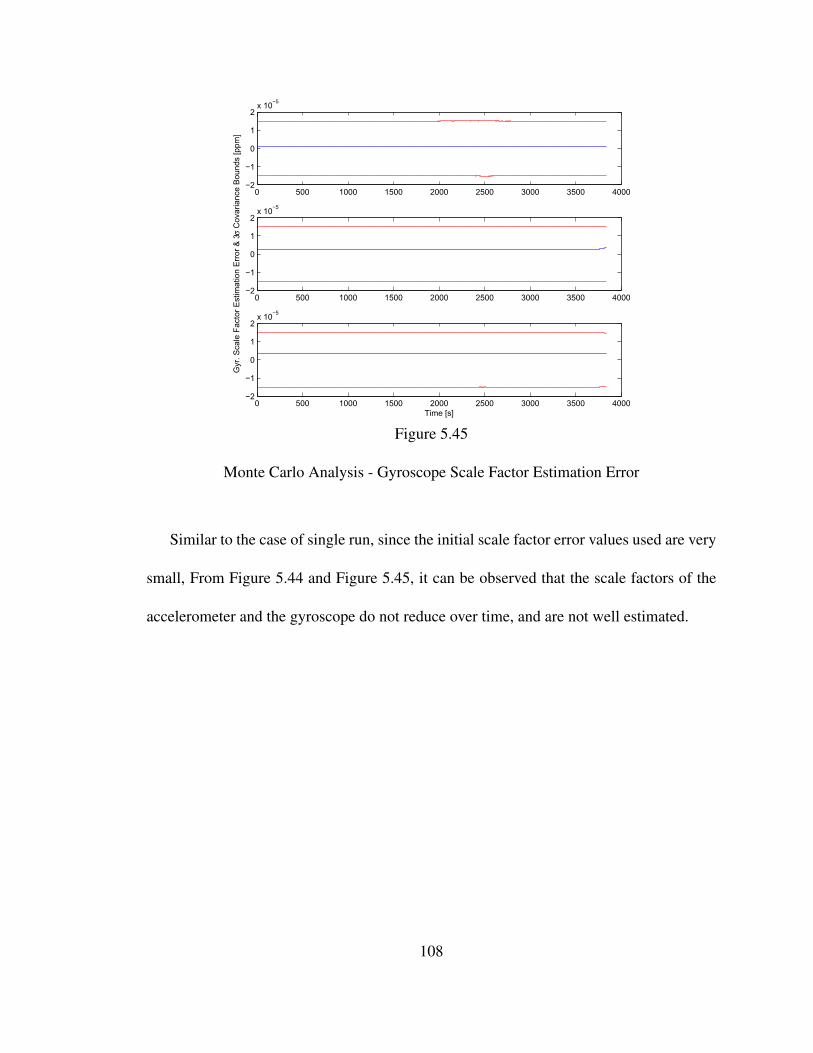
0 500 1000 1500 2000 2500 3000 3500 4000−2

−1

0

1

2x 10

−5

0 500 1000 1500 2000 2500 3000 3500 4000−2

−1

0

1

2x 10

−5

Gyr

. Sca

le F

acto

r E

stim

atio

n E

rror

& 3

σ C

ovar

ianc

e B

ound

s [p

pm]

0 500 1000 1500 2000 2500 3000 3500 4000−2

−1

0

1

2x 10

−5

Time [s]

Figure 5.45

Monte Carlo Analysis - Gyroscope Scale Factor Estimation Error

Similar to the case of single run, since the initial scale factor error values used are very

small, From Figure 5.44 and Figure 5.45, it can be observed that the scale factors of the

accelerometer and the gyroscope do not reduce over time, and are not well estimated.

108

CHAPTER 6

CONCLUSIONS

The navigation system is a critical component in the design of a spacecraft, and it is

important to have an on-board navigation algorithm to achieve precision landing. A de-

tailed analysis of a prototype navigation algorithm for precise lunar landing of a spacecraft

was developed and tested.

Using data from an STK scenario as the truth values, the navigation filter was tested

for the inertial navigation system and the integrated navigation system. From the results

obtained, it can be concluded that the INS alone does not result in precise landing of the

spacecraft due to build up of errors over time. The addition of aiding sensor measurements

to the INS highly improves the accuracy of the navigation filter. Analysis of the results also

show that, of the three aiding sensors, the terrain camera help achieve highest accuracy of

the navigation algorithm.

As observed from the results of the navigation filter, the bias errors of the accelerom-

eters and gyroscopes were well estimated while the scale factor errors were not well esti-

mated. The observability of the error variables is concluded to be dependent of the mag-

nitude of truth values of the bias and scale factors.

Through Monte Carlo analysis, a covariance analysis for the navigation filter was per-

formed. This analysis verifies that the filter provides accurate estimates of the position,

109

velocity and quaternion values. Also, the analysis shows that the bias of the IMU sensors

are well estimated, while the scale factors are not well estimated.

Since an early sensor activation provides improved navigation states for a longer por-

tion of the descent trajectory, it would be advantageous to enable the altimeter at an early

stage of the navigation scenario. This can improve the accuracy of the position and veloc-

ity estimates. Inclusion of more feature points enables early sensor activation, and helps

achieve higher accuracy of the navigation filter. Higher precision IMU’s also improve the

filter performance.

The accuracy of the initial state vector variables and truth value during the simulation

play an important role in the navigation filter. Also, the performance of the filter can be

improved as the sampling period of the measurement data is increased, as smaller time

periods avoid the buildup of the integration drift errors.

As the errors in the accelerometers and gyroscopes are not significant performance

drivers in the navigation filter, a reduced state vector might be realizable without reduced

navigation performance. This can also save computational power of the filter.

110

REFERENCES

[1] Pieters, C. M., Goswami, J. N., Clark, R. N., Annadurai, M., Boardman, J., Buratti,B., Combe, J. P., Dyar, M. D., Green, R., Head, J. W., Hibbitts, C., Hicks, M.,Isaacson, P., Klima, R., Kramer, G., Kumar, S., Livo, E., Lundeen, S., Malaret, E.,McCord, T., Mustard, J., Nettles, J., Petro, N., Runyon, C., Staid, M., Sunshine, J.,Taylor, L. A., Tompkins, S., and Varanasi, P., “Character and Spatial Distributionof OH/H2O on the Surface of the Moon Seen by M3 on Chandrayaan-1,” Science,Vol. 326, No. 5952, 2009, pp. 568–572.

[2] http://www.nrl.navy.mil/clementine2/.

[3] Tooley, C., “Lunar Reconnaissance Orbiter Spacecraft & Objectives,” Proceedingsof the 2006 AIAA-Houston Annual Technical Symposium, AIAA, Houston, TX, May2006.

[4] http://www.esa.int/SPECIALS/SMART-1/index.html.

[5] Ramos, R. H., Caramagno, A., Northey, D., Gittins, D., Riley, D., Portigliotti, S., andCapuano, M., “ExoMars Mission Analysis and Design - Entry, Descent and Land-ing,” Proceedings of the 17th AAS/AIAA Space Flight Mechanics Meeting, AAS,Sedona, AZ, January 2007.

[6] http://www.jspec.jaxa.jp/e/activity/selene2.html.

[7] Kubota, T., Hashimoto, T., Kawaguchi, J., Yano, H., Terui, F., Yoshikawa, M., Uo,M., and Shirakawa, K., “Guidance and Navigation Scheme for Hayabusa AsteroidExploration and Sample Return Mission,” The ESA Workshop on GNC for SmallBody Missions, ESA/ESTEC, Noordwijk, The Netherlands, January 2009.

[8] http://www.isro.gov.in/scripts/futureprogramme.aspx#Space.

[9] Shevchenko, V., “Russian project Luna-Glob: goals and status,” Geophysical Re-search Abstracts, Vol. 10, 2008.

[10] http://www.space.com/news/china-space-program-progress-sfn-100308.html.

[11] Farrell, J. A. and Barth, M., The Global Positioning System and Inertial Navigation,McGraw-Hill, New York, NY, 1998.

111

[12] Titterton, D. H. and Weston, J. L., Strapdown Inertial Navigation Technology, Amer-ican Institute of Aeronautics and Astronautics, Reston, VA, 2nd ed., 2004.

[13] Kluever, C. A., “Guidance Evaluation for Mars Precision Landing,” Proceedings ofthe 18th AAS/AIAA Space Flight Mechanics Meeting, AAS, Galveston, TX, January2008.

[14] Zanetti, R. and Bishop, R. H., “Adaptive Entry Navigation Using Inertial Measure-ments,” Proceedings of the 17th AAS/AIAA Space Flight Mechanics Meeting, AAS,Sedona, AZ, January 2007.

[15] Paschall II, S. C., Mars Entry Navigation Performance Analysis using Monte CarloAnalysis, Master’s thesis, Massachusetts Institute of Technology, Cambridge, MA,June 2002.

[16] Meditch, J. S., “On the Problem of Optimal Thrust Programming For a Lunar SoftLanding,” IEEE Transactions on Automatic Control, Vol. 9, No. 4, 1964, pp. 477–484.

[17] Betts, J. T., Practical Methods for Optimal Control Using Nonlinear Programming,Society for Industrial and Applied Mathematics, Philadelphia, PA, 2001.

[18] Hawkins, A. M., Fill, T. J., Proulx, R. J., and Feron, E. M. J., “Constrained TrajectoryOptimization for Lunar Landing,” Proceedings of the 16th AAS/AIAA Space FlightMechanics Meeting, AAS, Tampa, FL, January 2006.

[19] Cho, D. H., Jeong, B., Lee, D., and Bang, H., “Optimal Perilune Altitude of Lu-nar Landing Trajectory,” International Journal of Aeronautical & Space Sciences,Vol. 10, No. 1, 2009, pp. 67–74.

[20] Fisher, J. L. and Striepe, S. A., “Post2 End-To-End Descent and Landing Simulationfor the Autonomous Landing and Hazard Avoidance Technology project,” Proceed-ings of the 17th AAS/AIAA Space Flight Mechanics Meeting, AAS, Sedona, AZ,January 2007.

[21] Fernandez, J. G., Melloni, S., Matellano, P. C., and Graziano, M., “Optimal PreciseLanding for Lunar Missions,” Proceedings of the AIAA/AAS Astrodynamics Special-ist Conference and Exhibit, AIAA/AAS, Honolulu, HI, August 2008.

[22] Grewal, M. S., Weill, L. R., and Andrews, A. P., Global Positioning Systems, InertialNavigation, and Integration, John Wiley & Sons, Hoboken, NJ, 2nd ed., 2007.

[23] National Aeronautics and Space Administration, A Standardized Lunar CoordinateSystem for the Lunar Reconnaissance Orbiter, Goddard Space Flight Center, Green-belt, MD, May 2008.

[24] Chatfield, A. B., Fundamentals of High Accuracy Inertial Navigation, American In-stitute of Aeronautics and Astronautics, Reston, VA, 1997.

112

[25] Lyons III, L. W., “A New Method for the Alignment of Inertial Navigation Systems,”Journal of Aircraft, Vol. 9, No. 6, 1972, pp. 433–437.

[26] Savage, P. G., “Strapdown Inertial Navigation Integration Algorithm Design Part 1:Attitude Algorithms,” Journal of Guidance, Control, and Dynamics, Vol. 21, No. 1,1998, pp. 19–28.

[27] Savage, P. G., “Strapdown Inertial Navigation Integration Algorithm Design Part 2:Velocity and Position Algorithms,” Journal of Guidance, Control, and Dynamics,Vol. 21, No. 2, 1998, pp. 208–221.

[28] Litmanovich, Y. A., Lesyuchevsky, V. M., and Gusinsky, V. Z., “Two New Classes ofStrapdown Navigation Algorithms,” Journal of Guidance, Control, and Dynamics,Vol. 23, No. 1, 2000, pp. 34–44.

[29] Savage, P. G., “Analytical Modeling of Sensor Quantization in Strapdown InertialNavigation Error Equations,” Journal of Guidance, Control, and Dynamics, Vol. 25,No. 5, 2002, pp. 833–842.

[30] Levine, S. and Gelb, A., “Effect of Deflections of the Vertical on the Performance ofa Terrestrial Inertial Navigation System,” Journal of Spacecrafts and Rockets, Vol. 6,No. 9, 1969, pp. 978–984.

[31] DeMars, K. J., Precision Navigation for Lunar Descent and Landing, Master’s thesis,The University of Texas at Austin, Ausyin, TX, May 2007.

[32] Crassidis, J. L. and Junkins, J. L., Optimal Estimation of Dynamic Systems, Chapmanand Hall/CRC, Boca Raton, FL, 2004.

[33] Chobotov, V. A., Spacecraft Attitude Dynamics and Control, Krieger PublishingCompany, Malabar, FL, 1991.

[34] Crassidis, J. L., “Sigma-Point Kalman Filtering for Integrated GPS and Inertial Nav-igation,” IEEE Transactions on Aerospace and Electronic Systems, Vol. 42, No. 2,2006, pp. 750–756.

[35] Kani, A. N., Control Systems, RBA Publications, Chennai, India, 1998.

[36] Maybeck, P. S., Stochastic Models, Estimation, and Control, Vol. 1, Academic PressInc., New York, NY, 1979.

[37] Grewal, M. S. and Andrews, A. P., Kalman Filtering : Theory and Practice usingMATLAB, John Wiley & Sons, Hoboken, NJ, 3rd ed., 2008.

[38] Gelb, A., Kasper Jr., J. F., Nash Jr., R. A., Prince, C. F., and Sutherland Jr., A. A.,Applied Optimal Estimation, The M.I.T. Press, 1974.

113

[39] Wan, E. A. and van der Merwe, R., Kalman Filtering and Neural Networks, chap. 7,John Wiley & Sons, Hoboken, NJ, 2001.

[40] Wan, E. A., van der Merwe, R., and Julier, S. I., “Sigma-Point Kalman Filters forNonlinear Estimation and Sensor-Fusion - Applications to Integrated Navigation,”AIAA Guidance, Navigation, and Control Conference and Exhibit, Providence, RI,August 2004.

[41] Cohanim, B. E. and Collins, B. K., “Landing Point Designation Algorithm for LunarLanding,” Journal of Spacecraft and Rockets, Vol. 46, No. 4, 2009, pp. 858–864.

[42] Loucks, M. and Carrico, J., “The Astrogator’s Guild - Space Exploration EngineeringCorporation,” http://www.astrogatorsguild.com/.

114