on the observational determination of climate … (lindzen, 1999). ... in a recent paper (lindzen...

Asia-Pacific J. Atmos. Sci., 47(4), 377-390, 2011

DOI:10.1007/s13143-011-0023-x

On the Observational Determination of Climate Sensitivity and Its Implications

Richard S. Lindzen1 and Yong-Sang Choi

2

1Program in Atmospheres, Oceans, and Climate, Massachusetts Institute of Technology, Cambridge, U. S. A.

2Department of Environmental Science and Engineering, Ewha Womans University, Seoul, Korea

(Manuscript received 23 February 2011; revised 22 May 2011; accepted 22 May 2011)© The Korean Meteorological Society and Springer 2011

Abstract: We estimate climate sensitivity from observations, using

the deseasonalized fluctuations in sea surface temperatures (SSTs)

and the concurrent fluctuations in the top-of-atmosphere (TOA)

outgoing radiation from the ERBE (1985-1999) and CERES (2000-

2008) satellite instruments. Distinct periods of warming and cooling

in the SSTs were used to evaluate feedbacks. An earlier study

(Lindzen and Choi, 2009) was subject to significant criticisms. The

present paper is an expansion of the earlier paper where the various

criticisms are taken into account. The present analysis accounts for

the 72 day precession period for the ERBE satellite in a more

appropriate manner than in the earlier paper. We develop a method to

distinguish noise in the outgoing radiation as well as radiation

changes that are forcing SST changes from those radiation changes

that constitute feedbacks to changes in SST. We demonstrate that our

new method does moderately well in distinguishing positive from

negative feedbacks and in quantifying negative feedbacks. In contrast,

we show that simple regression methods used by several existing

papers generally exaggerate positive feedbacks and even show

positive feedbacks when actual feedbacks are negative. We argue that

feedbacks are largely concentrated in the tropics, and the tropical

feedbacks can be adjusted to account for their impact on the globe as

a whole. Indeed, we show that including all CERES data (not just

from the tropics) leads to results similar to what are obtained for the

tropics alone - though with more noise. We again find that the

outgoing radiation resulting from SST fluctuations exceeds the zero-

feedback response thus implying negative feedback. In contrast to

this, the calculated TOA outgoing radiation fluxes from 11 atmos-

pheric models forced by the observed SST are less than the zero-

feedback response, consistent with the positive feedbacks that

characterize these models. The results imply that the models are

exaggerating climate sensitivity.

Key words: Climate sensitivity, climate feedback, cloud, radiation,

satellite

1. Introduction

The heart of the global warming issue is so-called greenhouse

warming. This refers to the fact that the earth balances the heat

received from the sun (mostly in the visible spectrum) by

radiating in the infrared portion of the spectrum back to space.

Gases that are relatively transparent to visible light but strongly

absorbent in the infrared (greenhouse gases) interfere with the

cooling of the planet, forcing it to become warmer in order to

emit sufficient infrared radiation to balance the net incoming

sunlight (Lindzen, 1999). By net incoming sunlight, we mean that

portion of the sun’s radiation that is not reflected back to space by

clouds, aerosols and the earth’s surface. CO2, a relatively minor

greenhouse gas, has increased significantly since the beginning of

the industrial age from about 280 ppmv to about 390 ppmv,

presumably due mostly to man’s emissions. This is the focus of

current concerns. However, warming from a doubling of CO2

would only be about 1oC (based on simple calculations where the

radiation altitude and the Planck temperature depend on wave-

length in accordance with the attenuation coefficients of well-

mixed CO2 molecules; a doubling of any concentration in ppmv

produces the same warming because of the logarithmic depend-

ence of CO2’s absorption on the amount of CO

2) (IPCC, 2007).

This modest warming is much less than current climate models

suggest for a doubling of CO2. Models predict warming of from

1.5oC to 5oC and even more for a doubling of CO2. Model

predictions depend on the ‘feedback’ within models from the

more important greenhouse substances, water vapor and clouds.

Within all current climate models, water vapor increases with

increasing temperature so as to further inhibit infrared cooling.

Clouds also change so that their visible reflectivity decreases,

causing increased solar absorption and warming of the earth.

Cloud feedbacks are still considered to be highly uncertain

(IPCC, 2007), but the fact that these feedbacks are strongly

positive in most models is considered to be an indication that

the result is basically correct. Methodologically, this is unsatis-

factory. Ideally, one would seek an observational test of the

issue. Here we suggest that it may be possible to test the issue

with existing data from satellites.

Indeed, an earlier study by Forster and Gregory (2006)

examined the anomaly of the annual mean temperature and

radiative flux observed from a satellite. However, with the annual

time scale, the signal of short-term feedback associated with

water vapor and clouds can be contaminated by unknown time-

varying radiative forcing in nature, and the feedbacks cannot be

accurately diagnosed (Spencer, 2010). Moreover, as we will

show later in this paper, the regression approach, itself, is an

important source of bias. In a recent paper (Lindzen and Choi,

2009) we attempted to resolve these issues though, as has been

noted in subsequent papers, the details of that paper were, in

Corresponding Author: Prof. Yong-Sang Choi, Department of Environ-mental Science and Engineering, Ewha Womans University, Seoul 120-750 KoreaE-mail: [email protected].

378 ASIA-PACIFIC JOURNAL OF ATMOSPHERIC SCIENCES

important ways, also incorrect (Chung et al., 2010; Murphy,

2010; Trenberth et al., 2010). There were four major criticisms

to Lindzen and Choi (2009): (i) incorrect computation of climate

sensitivity, (ii) statistical insignificance of the results, (iii) misin-

terpretation of air-sea interaction in the Tropics, (iv) misuse of

uncoupled atmospheric models. The present paper responds to

the criticism, and corrects the earlier approach where appropriate.

The earlier results are not significantly altered, and we show why

these results differ from what others like Trenberth et al. (2010),

and Dessler (2010) obtain.

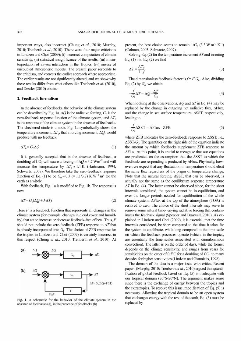
2. Feedback formalism

In the absence of feedbacks, the behavior of the climate system

can be described by Fig. 1a. ∆Q is the radiative forcing, G0 is the

zero-feedback response function of the climate system, and ∆T0

is the response of the climate system in the absence of feedbacks.

The checkered circle is a node. Fig. 1a symbolically shows the

temperature increment, ∆T0, that a forcing increment, ∆Q, would

produce with no feedback,

∆T0= G

0∆Q (1)

It is generally accepted that in the absence of feedback, a

doubling of CO2 will cause a forcing of ∆Q ≈ 3.7 Wm−2 and will

increase the temperature by ∆T0≈ 1.1 K (Hartmann, 1994;

Schwartz, 2007). We therefore take the zero-feedback response

function of Eq. (1) to be G0≈ 0.3 (= 1.1/3.7) K W−1 m2 for the

earth as a whole.

With feedback, Fig. 1a is modified to Fig. 1b. The response is

now

∆T= G0(∆Q + F∆T) (2)

Here F is a feedback function that represents all changes in the

climate system (for example, changes in cloud cover and humid-

ity) that act to increase or decrease feedback-free effects. Thus, F

should not include the zero-feedback (ZFB) response to ∆T that

is already incorporated into G0. The choice of ZFB response for

the tropics in Lindzen and Choi (2009) is certainly incorrect in

this respect (Chung et al., 2010; Trenberth et al., 2010). At

present, the best choice seems to remain 1/G0 (3.3 W m−2 K−1)

(Colman, 2003; Schwartz, 2007).

Solving Eq. (2) for the temperature increment ∆T and inserting

Eq. (1) into Eq. (2) we find

(3)

The dimensionless feedback factor is f = F G0 . Also, dividing

Eq. (2) by G0, we obtain

(4)

When looking at the observations, ∆Q and ∆T in Eq. (4) may be

replaced by the change in outgoing net radiative flux, ∆Flux,

and the change in sea surface temperature, ∆SST, respectively,

leading to

(5)

where ZFB indicates the zero-feedback response to ∆SST, i.e.,

∆SST/G0. The quantities on the right side of the equation indicate

the amount by which feedbacks supplement ZFB response to

∆Flux. At this point, it is crucial to recognize that our equations

are predicated on the assumption that the ∆SST to which the

feedbacks are responding is produced by ∆Flux. Physically, how-

ever, we expect that any fluctuation in temperature should elicit

the same flux regardless of the origin of temperature change.

Note that the natural forcing, ∆SST, that can be observed, is

actually not the same as the equilibrium response temperature

∆T in Eq. (4). The latter cannot be observed since, for the short

intervals considered, the system cannot be in equilibrium, and

over the longer periods needed for equilibration of the whole

climate system, ∆Flux at the top of the atmosphere (TOA) is

restored to zero. The choice of the short intervals may serve to

remove some natural time-varying radiative forcing that contam-

inates the feedback signal (Spencer and Braswell, 2010). As ex-

plained in Lindzen and Choi (2009), it is essential, that the time

intervals considered, be short compared to the time it takes for

the system to equilibrate, while long compared to the time scale

on which the feedback processes operate (which, in the tropics,

are essentially the time scales associated with cumulonimbus

convection). The latter is on the order of days, while the former

depends on the climate sensitivity, and ranges from years for

sensitivities on the order of 0.5oC for a doubling of CO2 to many

decades for higher sensitivities (Lindzen and Giannitsis, 1998).

The domain of the data is a major issue with critics. Recent

papers (Murphy, 2010; Trenberth et al., 2010) argued that quanti-

fication of global feedback based on Eq. (5) is inadequate with

our tropical domain (20°S-20°N). The argument makes sense

since there is the exchange of energy between the tropics and

the extratropics. To resolve this issue, modification of Eq. (5) is

necessary. Allowing the tropical domain to be an open system

that exchanges energy with the rest of the earth, Eq. (5) must be

replaced by

∆T∆T0

1 f–---------=

f

G0

------– ∆T ∆Q∆T

G0

-------–=

f

G0

------– ∆SST ∆Flux ZFB–=

Fig. 1. A schematic for the behavior of the climate system in theabsence of feedbacks (a), in the presence of feedbacks (b).

31 August 2011 Richard S. Lindzen and Yong-Sang Choi 379

(6)

where the factor c results from the sharing of the tropical

feedbacks over the globe, following the methodology of Lindzen,

Chou and Hou (2001), (hereafter LCH01) and Lindzen, Hou and

Farrell (1982), The methodology developed in LCH01 permits

the easy evaluation of the contribution of tropical processes to the

global value. As noted by LCH01, this does not preclude there

being extratropical contributions as well. In fact, with the global

data (available for a limited period only), the factor c is estimated

to be close to unity, so that Eq. (6) is similar to Eq. (5); based on

the independent analysis with the global data (Choi et al., 2011,

manuscript submitted to Meteorology and Atmospheric Physics)

(results from which will be presented later in this paper), it is

clear that the use of the global data essentially leads to similar

results to that from the tropical data. This similarity is probably

due to the concentration of water vapor in the tropics (more

details are given in Section 6). With the tropical data in this study,

the factor c is simply set to 2; that is to say that the contribution of

the tropical feedback to the global feedback is only about half of

the tropical feedback. However, we also tested various c values

1.5 to 3 (viz Section 6); as we will show, the precise choice of

this factor c does not affect the major conclusions of this study.

From Eq. (6), the longwave (LW) and shortwave

(7a)

(7b)

Here we can identify ∆Flux as the change in outgoing long-

wave radiation (OLR) and shortwave radiation (SWR) measured

by satellites associated with the measured ∆SST. Since we know

the value of G0, the experimentally determined slope (the

quantity on the right side of Eq. (7)) allows us to evaluate the

magnitude and sign of the feedback factor f provided that we also

know the value of the ZFB response (∆SST/G0 in this study).

For observed variations, the changes in radiation (associated for

example with volcanoes or non-feedback changes in clouds) can

cause changes in SST as well as respond to changes in SST, and

there is a need to distinguish these two possibilities. This is less

of an issue with model results from AMIP (Atmospheric Model

Intercomparison Project) where observed variations in SST are

specified. Of course, there is always the problem of noise arising

from the fact that clouds depend on factors other than surface

temperature, and this is true for AMIP as well as for nature.

Note that the noise turns out to be generally greater for larger

domains that include the extratropics as well as land. Note as

well that this study deals with observed outgoing fluxes, but

does not specifically identify the origin of the changes.

3. The data and their problems

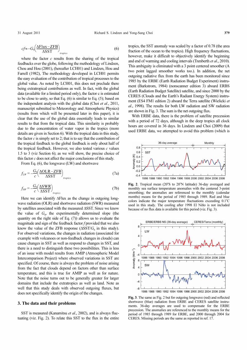
SST is measured (Kanamitsu et al., 2002), and is always fluc-

tuating (viz. Fig. 2). To relate this SST to the flux in the entire

tropics, the SST anomaly was scaled by a factor of 0.78 (the area

fraction of the ocean to the tropics). High frequency fluctuations,

however, make it difficult to objectively identify the beginning

and end of warming and cooling intervals (Trenberth et al., 2010).

This ambiguity is eliminated with a 3 point centered smoother (A

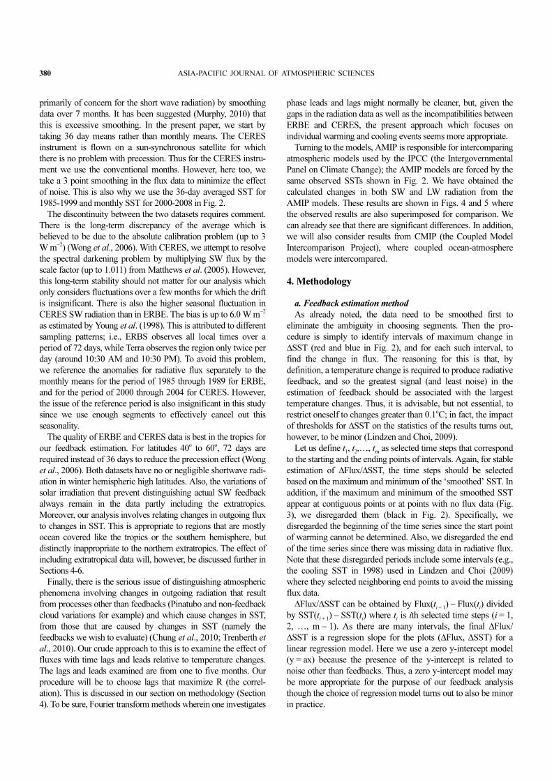
two point lagged smoother works too.). In addition, the net

outgoing radiative flux from the earth has been monitored since

1985 by the ERBE (Earth Radiation Budget Experiment) instru-

ment (Barkstrom, 1984) (nonscanner edition 3) aboard ERBS

(Earth Radiation Budget Satellite) satellite, and since 2000 by the

CERES (Clouds and the Earth’s Radiant Energy System) instru-

ment (ES4 FM1 edition 2) aboard the Terra satellite (Wielicki et

al., 1998). The results for both LW radiation and SW radiation

are shown in Fig. 3. The sum is the net outgoing flux.

With ERBE data, there is the problem of satellite precession

with a period of 72 days, although in the deep tropics all clock

hours are covered in 36 days. In Lindzen and Choi (2009) that

used ERBE data, we attempted to avoid this problem (which is

cf G0–∆Flux ZFB–

∆SST-------------------------------⎝ ⎠⎛ ⎞

tropics

≈

fLWG0

c------–

∆OLR ZFB–

∆SST--------------------------------⎝ ⎠⎛ ⎞

tropics

=

fSWG0

c------–

∆SWR

∆SST-----------------⎝ ⎠⎛ ⎞

tropics

=Fig. 2. Tropical mean (20

oS to 20

oN latitude) 36-day averaged and

monthly sea surface temperature anomalies with the centered 3-pointsmoothing; the anomalies are referenced to the monthly (calendarmonths) means for the period of 1985 through 1989. Red and bluecolors indicate the major temperature fluctuations exceeding 0.1o

Cused in this study. The cooling after 1998 El Niño is not includedbecause of no flux data is available for this period (viz. Fig. 3).

Fig. 3. The same as Fig. 2 but for outgoing longwave (red) and reflectedshortwave (blue) radiation from ERBE and CERES satellite instru-ments. 36-day averages are used to compensate for the ERBEprecession. The anomalies are referenced to the monthly means for theperiod of 1985 through 1989 for ERBE, and 2000 through 2004 forCERES. Missing periods are the same as reported in ref. 17.


primarily of concern for the short wave radiation) by smoothing

data over 7 months. It has been suggested (Murphy, 2010) that

this is excessive smoothing. In the present paper, we start by

taking 36 day means rather than monthly means. The CERES

instrument is flown on a sun-synchronous satellite for which

there is no problem with precession. Thus for the CERES instru-

ment we use the conventional months. However, here too, we

take a 3 point smoothing in the flux data to minimize the effect

of noise. This is also why we use the 36-day averaged SST for

1985-1999 and monthly SST for 2000-2008 in Fig. 2.

The discontinuity between the two datasets requires comment.

There is the long-term discrepancy of the average which is

believed to be due to the absolute calibration problem (up to 3

W m−2) (Wong et al., 2006). With CERES, we attempt to resolve

the spectral darkening problem by multiplying SW flux by the

scale factor (up to 1.011) from Matthews et al. (2005). However,

this long-term stability should not matter for our analysis which

only considers fluctuations over a few months for which the drift

is insignificant. There is also the higher seasonal fluctuation in

CERES SW radiation than in ERBE. The bias is up to 6.0 W m−2

as estimated by Young et al. (1998). This is attributed to different

sampling patterns; i.e., ERBS observes all local times over a

period of 72 days, while Terra observes the region only twice per

day (around 10:30 AM and 10:30 PM). To avoid this problem,

we reference the anomalies for radiative flux separately to the

monthly means for the period of 1985 through 1989 for ERBE,

and for the period of 2000 through 2004 for CERES. However,

the issue of the reference period is also insignificant in this study

since we use enough segments to effectively cancel out this

seasonality.

The quality of ERBE and CERES data is best in the tropics for

our feedback estimation. For latitudes 40o to 60o, 72 days are

required instead of 36 days to reduce the precession effect (Wong

et al., 2006). Both datasets have no or negligible shortwave radi-

ation in winter hemispheric high latitudes. Also, the variations of

solar irradiation that prevent distinguishing actual SW feedback

always remain in the data partly including the extratropics.

Moreover, our analysis involves relating changes in outgoing flux

to changes in SST. This is appropriate to regions that are mostly

ocean covered like the tropics or the southern hemisphere, but

distinctly inappropriate to the northern extratropics. The effect of

including extratropical data will, however, be discussed further in

Sections 4-6.

Finally, there is the serious issue of distinguishing atmospheric

phenomena involving changes in outgoing radiation that result

from processes other than feedbacks (Pinatubo and non-feedback

cloud variations for example) and which cause changes in SST,

from those that are caused by changes in SST (namely the

feedbacks we wish to evaluate) (Chung et al., 2010; Trenberth et

al., 2010). Our crude approach to this is to examine the effect of

fluxes with time lags and leads relative to temperature changes.

The lags and leads examined are from one to five months. Our

procedure will be to choose lags that maximize R (the correl-

ation). This is discussed in our section on methodology (Section

4). To be sure, Fourier transform methods wherein one investigates

phase leads and lags might normally be cleaner, but, given the

gaps in the radiation data as well as the incompatibilities between

ERBE and CERES, the present approach which focuses on

individual warming and cooling events seems more appropriate.

Turning to the models, AMIP is responsible for intercomparing

atmospheric models used by the IPCC (the Intergovernmental

Panel on Climate Change); the AMIP models are forced by the

same observed SSTs shown in Fig. 2. We have obtained the

calculated changes in both SW and LW radiation from the

AMIP models. These results are shown in Figs. 4 and 5 where

the observed results are also superimposed for comparison. We

can already see that there are significant differences. In addition,

we will also consider results from CMIP (the Coupled Model

Intercomparison Project), where coupled ocean-atmosphere

models were intercompared.

4. Methodology

a. Feedback estimation method

As already noted, the data need to be smoothed first to

eliminate the ambiguity in choosing segments. Then the pro-

cedure is simply to identify intervals of maximum change in

∆SST (red and blue in Fig. 2), and for each such interval, to

find the change in flux. The reasoning for this is that, by

definition, a temperature change is required to produce radiative

feedback, and so the greatest signal (and least noise) in the

estimation of feedback should be associated with the largest

temperature changes. Thus, it is advisable, but not essential, to

restrict oneself to changes greater than 0.1oC; in fact, the impact

of thresholds for ∆SST on the statistics of the results turns out,

however, to be minor (Lindzen and Choi, 2009).

Let us define t1, t

2,…, t

m as selected time steps that correspond

to the starting and the ending points of intervals. Again, for stable

estimation of ∆Flux/∆SST, the time steps should be selected

based on the maximum and minimum of the ‘smoothed’ SST. In

addition, if the maximum and minimum of the smoothed SST

appear at contiguous points or at points with no flux data (Fig.

3), we disregarded them (black in Fig. 2). Specifically, we

disregarded the beginning of the time series since the start point

of warming cannot be determined. Also, we disregarded the end

of the time series since there was missing data in radiative flux.

Note that these disregarded periods include some intervals (e.g.,

the cooling SST in 1998) used in Lindzen and Choi (2009)

where they selected neighboring end points to avoid the missing

flux data.

∆Flux/∆SST can be obtained by Flux(ti + 1) − Flux(ti) divided

by SST(ti + 1) − SST(ti) where ti is ith selected time steps (i = 1,

2, …, m − 1). As there are many intervals, the final ∆Flux/

∆SST is a regression slope for the plots (∆Flux, ∆SST) for a

linear regression model. Here we use a zero y-intercept model

(y = ax) because the presence of the y-intercept is related to

noise other than feedbacks. Thus, a zero y-intercept model may

be more appropriate for the purpose of our feedback analysis

though the choice of regression model turns out to also be minor

in practice.


One must also distinguish ∆SST’s that are forcing changes in

∆Flux, from responses to ∆Flux. Otherwise, ∆Flux/∆SST can

have fluctuations (as found by Dessler, 2010 and Trenberth et al.,

2010, for example) that may not represent feedbacks that we

wish to determine. The results from Trenberth et al. (2010) and

Dessler (2010) were, in fact, ambiguous as well because of the

very low correlation of their regression of ∆F on ∆SST. To avoid

the causality problem, we use a lag-lead method (e.g., use of

Flux(t + lag) and SST(t)) for ERBE 36-day and CERES monthly

smoothed data). In general, the use of leads for flux will

emphasize forcing by the fluxes, and the use of lags will

emphasize responses by the fluxes to changes in SST.

The above procedures help to obtain a more accurate and

objective climate feedback factor than the use of original monthly

data. As we will show below, this was tested by a Monte-Carlo

test of a simple feedback-forcing model.

b. Simple model analysis

Following Spencer and Braswell (2010), we assume an

hypothetical climate system with uniform temperature and heat

capacity, for which SST and forcing are time-varying. Then the

model equation of the system is

(8)

where Cp is the bulk heat capacity of the system (14 yr W m−2

K−1 in this study, from Schwartz, 2007); ∆SST is SST deviation

away from an equilibrium state of energy balance; F is the

feedback function that is the same as the definition in Eq. (2); Q

is any forcing that changes SST (Forster and Gregory, 2006;

Spencer and Braswell, 2010). Q consists in three components: (i)

Q1= external radiative forcing (e.g., from anthropogenic green-

house gas emission), (ii) Q2= internal non-radiative forcing (from

heat transfer from the ocean, for example), and (iii) Q3= internal

CPd∆SST

dt----------------- Q t( ) F ∆SST t( )⋅–=

Fig. 4. Comparison of outgoing longwave radiation from AMIP models (black) and the observations (red) shown in Fig. 3.


radiative forcing (e.g., from water vapor or clouds.). Among the

three forcings, the two external and internal ‘radiative’ forcings,

and F⋅∆SST(t) constitute TOA net radiative flux anomaly; i.e.,

∆Flux = F⋅∆SST(t) − [Q1(t) + Q

3(t)].

The model system was basically forced by random internal

non-radiative forcing changing SST (ie, Q2). The system was also

forced by random internal radiative forcing (ie, Q3). For this

preliminary test, normally distributed random numbers with zero

mean were inserted into Q1 and Q

2.; we anticipate using forcing

with realistic atmospheric or oceanic spectra in future tests. Here

the variance of internal non-radiative forcing is set to 5 and the

variance of internal radiative forcing is set to 0.7. Hence, the ratio

of variances of the two forcings is 14% (hereafter the noise

level). These settings generally give simulated ∆SST and ∆Flux

with similar variances to the observed, The simulated variances

are, however, subject to model representation as well. Finally

the system was additionally forced by transient external radiative

forcing (0.4 W m−2 per decade due to increasing CO2) (Spencer

and Braswell, 2010). Integration is done at monthly time steps*.

We used Runge-Kutta 4th order method for numerical solution of

randomly forced system, Eq. (8) (Machiels and Deville, 1998).

Figure 6 compares the simple regression method and our method

for the feedback function F = 6 W m−2 K−1 (it indicates negative

feedback as it is larger than Planck response 3.3 W m−2 K−1). The

maximum R occurs at small (zero or a month) lag and the corres-

ponding ∆Flux/∆SST (5.7 W m−2 K−1) is close to the assumed F

(6 W m−2 K−1), whereas the simple regression method underesti-

mates F (3.2 W m−2 K−1).

The difference between the simple regression and our method

is statistically significant by a Monte-Carlo test (10,000 repeti-

Fig. 5. Comparison of reflected shortwave radiation from AMIP models (black) and the observations (blue) shown in Fig. 3.

*It is also possible to integrate at daily time steps, and degrade the time series to the monthly averages without significantly changing theresults - suggesting that the coarser time resolution is adequate for our purposes.


tions). Figure 7 shows the probability density functions of the

estimated ∆Flux/∆SST, and compares with the three true F

values (1, 3.3, and 6 W m−2 K−1) that were specified for the

model. We do not rule out the possibilities that both methods fail

to estimate the actual feedback (the tail of the density functions),

but we see clearly that the simple regression always undere-

stimates negative feedbacks and exaggerates positive feedbacks.

This is seen more clearly in Table 1 which shows the central

values of gain and feedback factors for both the simple

regressions and for the lag-lead approach (LC). The simple

regression even finds fairly large positive feedbacks when the

actual feedback is negative. This bias is, at least, partially because

the simple regression includes time intervals that approach

equilibration time, and at equilibrium, we would have a ∆SST

with no ∆Flux.

By contrast, our method shows moderately good performance

for estimating the feedback parameter especially for significant

negative feedbacks (comparable to what we observe in the data).

Fig. 6. Comparison between simple regression method and the methodused in this study, based on simple model results for F = 6 Wm−2 K−1.

Fig. 7. Probability density function of simple model simulation results(10,000 repeats) for the feedback parameter F = 1, 3.3, and 6 Wm−2

K−1

(blue dotted line). The black line is from the simple regression, and thered line is from the methodology in this study. Note that, in the case of'true' positive feedback, the LC method shows an insignificant indica-tion of a negative feedback. The means of the lags with maximum Rselected in our method are also noted.


The system with smaller F generates the sinusoidal shape of the

slopes with respect to lags, so that it turns out to have maximum

R at larger lag. In this case, the estimated climate feedbacks are

the lagged response though estimates are less reliable than when

maximum R occurs at near-zero lag (Fig. 8). Therefore, for the

system with smaller F our method is less efficient, and the true

value is in between the simple regression and our method. This

is also the case for the system with the same F with an increased

noise level (Fig. 8). That is to say, the longer the lag needed to

maximize R, the more our method overestimates F. This may be

because the lagged response is attributed to both feedback and

noise, and heavier noise at longer lag unduly raises the slope.

Regardless of feedback strength, with either no internal (cloud-

induced) radiative change or the prescribed temperature vari-

ation, ∆Flux/∆SST at zero lag (with maximum R) is always

identical to the assumed F. Thus AMIP systematically shows

maximum R at zero lag, while CMIP does not; thus, the use of

AMIP seems more appropriate in estimating model feedback

than the use of CMIP.

An example of a comparison of simple regression with our

lead-lag approach is taken from Choi et al. (2011, manuscript

submitted to Meteorology and Atmospheric Physics) with slight

modification. Here we compared the use of the simple re-

gression approach with our approach for the complete CERES

data set used by Dessler (2010). The results are shown in Fig. 9

where we show the impact of using segments (as opposed to the

continuous record as was done by Dessler, 2010) and the use of

lead-lag as opposed to simple regression. The former serves

mainly to greatly increase the correlation (r2) from the negligible

value obtained by Dessler (2010); the latter leads to a significant

negative feedback as opposed to the weak and insignificant

positive feedback claimed by Dessler (2010). We will discuss

these results later in connection with our emphasis on tropical

data. Recall, that this example considers data from all latitudes

covered by CERES. However, it should be emphasized that

even Dessler’s treatment of the data leads to negative feedback

Table 1. Summary of simple model simulation results shown in Fig. 7.The gain is 1/G

0 divided by the averaged F. Note that the averaged F is

larger than the value of the most frequent occurrence for the simpleregression method.

True values LC Simple regression

Gain f Gain f Gain f

0.55 −0.80 0.52 −0.92 0.66 −0.51

1.00 0.00 0.83 −0.21 1.42 0.29

3.30 0.68 1.53 0.34 23.57 0.94

Fig. 8. The relationship between the estimated feedback parameter F,the lags with maximum R, and the noise level (in %).

Fig. 9. The lagged regression slopes and their one-σ uncertainties of∆Flux versus ∆SST from CERES and ECMWF interim data used inDessler (2010). Note that here ∆Flux is 'global' radiative flux variationby clouds, and a positive ∆Flux/∆SST means a negative cloudfeedback. ∆Flux and ∆SST values are calculated by taking (black)original monthly anomaly data, and (red) the method in this study; thenumbers indicate lagged linear correlation coefficients.


when lags are considered.

5. Results

a. Climate sensitivity from observations and comparison to

AMIP models

Given the above, it is now possible to directly test the ability of

models to adequately simulate the sensitivity of climate (see

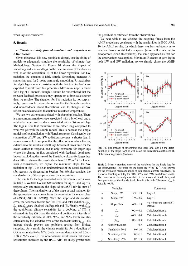
Methodology, Section 4). Figure 10 shows the impact of

smoothing and leads and lags on the determination of the slope as

well as on the correlation, R, of the linear regression. For LW

radiation, the situation is fairly simple. Smoothing increases R

somewhat, and for 3 point symmetric smoothing, R maximizes

for slight lag or zero - consistent with the fact that feedbacks are

expected to result from fast processes. Maximum slope is found

for a lag of 1 ‘month’, though it should be remembered that the

relevant feedback processes may operate on a time scale shorter

than we resolve. The situation for SW radiation is, not surpris-

ingly, more complex since phenomena like the Pinatubo eruption

and non-feedback cloud fluctuations lead to changes in SW

reflection and associated fluctuations in surface temperature.

We see two extrema associated with changing lead/lag. There

is a maximum negative slope associated with a brief lead, and a

relatively large positive slope associated with a 3-4 month lag.

The lags in SW that maximize R are rather long compared to

what we get with the simple model. This is because the simple

model is of total radiation with Planck response. Consistently, the

summation of LW and SW radiations presents a shorter lag. It

seems reasonable to suppose that the effect of anomalous forcing

extends into the results at small lags because it takes time for the

ocean surface to respond, and is only overcome for larger lags

where the change in flux associated with feedback dominates.

Indeed, excluding the case of the Pinatubo volcano for larger lags

does little to change the results (less than 0.3 W m−2 K−1). Under

such circumstances, we expect the maximum slope for SW

radiation in Fig. 10 to be an underestimate of the actual feedback

(for reasons we discussed in Section 4b). We also consider the

standard error of the slope to show data uncertainty.

The results for the lags associated with maximum R are shown

in Table 2. We take LW and SW radiation for lag = 1 and lag = 3,

respectively, and measure the slope ∆Flux/∆SST for the sum of

these fluxes. The standard error of the slope in total radiation for

the appropriate lags comes from the regression for scatter plots

of (∆SST, ∆(OLR + SWR)). With the slope and its standard

error, the feedback factors for LW, SW, and total radiation (fSW

,

fLW

, and fTotal

) are obtained via Eqs. (6) and (7). Finally, with fTotal

,

the equilibrium climate sensitivity for a doubling of CO2 is

obtained via Eq. (3). Here the statistical confidence intervals of

the sensitivity estimate at 90%, 95%, and 99% levels are also

calculated by the standard error of the feedback factor fTotal

. This

interval should prevent any problems arising from limited

sampling. As a result, the climate sensitivity for a doubling of

CO2 is estimated to be 0.7K (with the confidence interval 0.5K -

1.3K at 99% levels). This observational result shows that model

sensitivities indicated by the IPCC AR4 are likely greater than

the possibilities estimated from the observations.

We next wish to see whether the outgoing fluxes from the

AMIP models are consistent with the sensitivities in IPCC AR4.

To the AMIP results, for which there was less ambiguity as to

whether fluxes constituted a response (noise still exists due to

autonomous cloud fluctuations), the same approach as that for

the observations was applied. Maximum R occurs at zero lag in

both LW and SW radiation, so we simply chose the AMIP

Fig. 10. The impact of smoothing and leads and lags on the deter-mination of the slope (top) as well as on the correlation coefficient, R,of the linear regression (bottom).

Table 2. Mean ± standard error of the variables for the likely lag forthe observations. The units for the slope are W m

−2K

−1. Also shown

are the estimated mean and range of equilibrium climate sensitivity (inK) for a doubling of CO

2 for 90%, 95%, and 99% confidence levels.

The numbers are basically calculated to the second decimal place, andthen presented as the first decimal place in this table. The mean f

Total is

actually −0.54.

Variables Comments

a Slope, LW 5.3 ± 1.3 Lag = 1

b Slope, SW 1.9 ± 2.6 Lag = 3

c Slope, Total 6.9 ± 1.8= a + b for the same SST interval

d fLW

−0.3 ± 0.2 Calculated from a

e fSW

−0.3 ± 0.4 Calculated from b

f fTotal

−0.5 ± 0.3 Calculated from c

g Sensitivity, mean 0.7 Calculated from f

h Sensitivity, 90% 0.6-1.0 Calculated from f

i Sensitivity, 95% 0.5-1.1 Calculated from f

j Sensitivity, 99% 0.5-1.3 Calculated from f


fluxes without lag. The results are shown in Table 3. In contrast

to the observed fluxes, the implied feedbacks in the models are

all positive, and in one case, marginally unstable. Given the

uncertainties, however, one should not take that too seriously.

Table 4 compares the climate sensitivities in degrees K for a

doubling of CO2 implied by feedback factors f in Table 3 with

those in IPCC AR4. To indicate statistical significance of our

results obtained from limited sampling, we also calculated the

confidence intervals of the climate sensitivity using the standard

errors of f in Table 3. All the sensitivities in IPCC AR4 are

within the 90% confidence intervals of our sensitivity estimates.

The agreement does not seem notable, but this is because, for

positive feedbacks, sensitivity is strongly affected by small

changes in f that are associated standard errors in Table 3.

Consequently, the confidence intervals include “infinity”. This is

seen in Fig. 11 in the pink region. It has, in fact, been suggested

by Roe and Baker (2007), that this sensitivity of the climate

sensitivity to uncertainty in the feedback factor is why there has

been no change in the range of climate sensitivities indicated by

GCMs since the 1979 Charney Report (1979). By contrast, in

the green region, which corresponds to the observed feedback

factors, sensitivity is much better constrained.

While the present analysis is a direct test of feedback factors, it

does not provide much insight into detailed mechanism.

Nevertheless, separating the contributions to f from long wave

and short wave fluxes provides some interesting insights. The

results are shown in Tables 2 and 3. It should be noted that the

consideration of the zero-feedback response, and the tropical

feedback factor to be half of the global feedback factor is

actually necessary for our measurements from the Tropics;

Table 3. Regression statistics between ∆Flux and ∆SST and the estimated feedback factors (f) for LW, SW, and total radiation in AMIP models; theslope is ∆Flux/∆SST, N is the number of the points or intervals, R is the correlation coefficient, and SE is the standard error of ∆Flux/∆SST.

LW SW LW + SW

N Slope R SE fLW

Slope R SE fSW

Slope R SE f

CCSM3 17 1.2 0.4 2.0 0.3 −3.7 −0.9 1.0 0.6 −2.5 −0.5 2.2 0.9

ECHAM5/MPI-OM 16 1.1 0.4 1.6 0.3 −0.1 0.0 1.9 0.0 1.0 0.3 2.1 0.3

FGOALS-g1.0 16 0.4 0.2 1.2 0.4 −2.8 −0.8 1.0 0.4 −2.4 −0.6 1.4 0.9

GFDL-CM2.1 16 2.1 0.8 0.9 0.2 −2.1 −0.4 2.4 0.3 0.0 0.0 2.0 0.5

GISS-ER 21 3.2 0.8 1.1 0.0 −3.7 −0.6 1.8 0.6 −0.5 −0.1 1.3 0.6

INM-CM3.0 23 2.7 0.6 1.4 0.1 −3.4 −0.7 1.3 0.5 −0.7 −0.1 1.8 0.6

IPSL-CM4 21 −0.4 −0.1 1.1 0.6 −2.3 −0.5 1.6 0.3 −2.7 −0.5 1.7 0.9

MRI-CGCM2.3.2 21 −0.8 −0.3 1.3 0.6 −3.8 −0.6 2.5 0.6 −4.7 −0.7 2.5 1.2

MIROC3.2(hires) 21 2.4 0.6 1.4 0.1 −2.4 −0.7 1.4 0.4 0.0 0.0 1.3 0.5

MIROC3.2(medres) 21 3.4 0.8 1.0 0.0 −3.6 −0.7 2.0 0.5 −0.3 −0.1 1.6 0.5

UKMO-HadGEM1 17 4.4 0.8 2.2 −0.2 −3.6 −0.7 1.5 0.5 0.8 0.2 2.1 0.4

Table 4. Comparison of model equilibrium climate sensitivities (in K) for a doubling of CO2 defined from IPCC AR4 and estimated from feedback

factors in this study. The obvious difference between two columns labeled ‘sensitivity’ is discussed in more detail in the last paragraph of section 3.1.The estimated climate sensitivities for models as well as their confidence intervals are given for 90%, 95%, and 99% confidence levels.

Models IPCC AR4 Estimate in this study

Sensitivity Sensitivity Confidence interval of sensitivity

90% 95% 99%

CCSM3 2.7 8.1 1.6 - Infinity 1.4 - Infinity 1.1 - Infinity

ECHAM5/MPI-OM 3.4 1.7 0.9 - 8.0 0.9 - 28.2 0.8 - Infinity

FGOALS-g1.0 2.3 7.9 2.2 - Infinity 2.0 - Infinity 1.6 - Infinity

GFDL-CM2.1 3.4 2.2 1.1 - 351.4 1.0 - Infinity 0.8 - Infinity

GISS-ER 2.7 2.5 1.5 - 8.7 1.4 - 16.4 1.2 - Infinity

INM-CM3.0 2.1 2.7 1.3 - Infinity 1.2 - Infinity 1.0 - Infinity

IPSL-CM4 4.4 10.4 2.1 - Infinity 1.8 - Infinity 1.4 - Infinity

MRI-CGCM2.3.2 3.2 Infinity 2.5 - Infinity 2.0 - Infinity 1.4 - Infinity

MIROC3.2(hires) 4.3 2.2 1.3 - 6.4 1.2 - 10.0 1.1 - Infinity

MIROC3.2(medres) 4 2.4 1.3 - 14.7 1.2 - Infinity 1.0 - Infinity

UKMO-HadGEM1 4.4 1.7 1.0 - 8.8 0.9 - 38.9 0.8 - Infinity


however, these were not considered in Lindzen and Choi (2009).

Accordingly, with respect to separating longwave and shortwave

feedbacks, the interpretation by Lindzen and Choi (2009) needs

to be corrected. These tables show recalculated feedback factors

in the presence of the zero-feedback Planck response. The

negative feedback from observations is from both longwave and

shortwave radiation, while the positive feedback from models is

usually but not always from longwave feedback.

As concerns the infrared, there is, indeed, independent

evidence for a positive water vapor feedback (Soden et al., 2005),

but, if this is true, this feedback is presumably cancelled by a

negative infrared feedback such as that proposed by LCH01 on

the iris effect. In the models, on the contrary, the long wave

feedback appears to be positive (except for two models), but it is

not as great as expected for the water vapor feedback (Colman,

2003; Soden et al., 2005). This is possibly because the so-called

lapse rate feedback as well as negative longwave cloud feedback

acting to cancel some of the TOA OLR feedback in current

models. Table 3 implies that TOA longwave and shortwave

contributions are coupled in models (the correlation coefficient

between fLW

and fSW

from models is about −0.5.). This coupling

most likely is associated with the primary clouds in models -

optically thick high-top clouds (Webb et al., 2006). In most

climate models, the feedbacks from these clouds are simulated to

be negative in longwave and strongly positive in shortwave, and

dominate the entire model cloud feedback (Webb et al., 2006).

Therefore, the cloud feedbacks may also serve to contribute to

the negative OLR feedback and the positive SWR feedback.

New spaceborne data from the CALIPSO lidar (CALIOP; Winker

et al., 2007) and the CloudSat radar (CPR; Im et al., 2005)

should provide a breakdown of cloud behavior with altitude

which may give some insight into what actually is contributing to

the radiation.

b. Comparison to CMIP models and their limitations

It has been argued that CMIP models are more appropriate for

the present purpose since the uncoupled AMIP models are

prescribed with incomplete forcings of SST (Trenberth et al.,

2010). However, it is precisely for this reason that AMIP models

are preferred for feedback estimates. Note that we are considering

atmospheric feedbacks to SST fluctuations. As already seen, in

analyzing observed behavior, the presence of SST variations that

are primarily caused by atmospheric changes (from volcanoes,

non-feedback cloud variations, etc.) leads to difficulty in distin-

guishing SST variations that are primarily forcing atmospheric

changes (i.e., feedbacks). This situation is much simpler with

AMIP results since we can be sure that SST variations (which

are forced to be the same as observed SST) cannot respond to

atmospheric changes. The fact that CMIP SST variations are

significantly different from observed SST variations further

makes it unlikely that the model atmospheric processes are

implicitly forcing the SST’s used for AMIP. Note that important

ocean phenomena such as El Niño-Southern Oscillation and

Pacific Decadal Oscillation are generally misrepresented by

CMIP models. As noted, AMIP results are still subject to noise

since outgoing radiation includes changes associated with non-

feedback cloud variations.

In applying our methodology to CMIP, we see that coupled

models differ in the behavior of SST, and the intervals of SST

must be selected differently for different models. Some models

have much smaller variability of SST than nature and only a few

intervals of SST could be selected. As we see in Fig. 12, the

CMIP results (black dots) display behavior somewhat similar to

ERBE and CERES results (red open circles) with respect to

lags. However, when identifying each number, we found that the

results are quantitatively ambiguous. The slope ∆OLR/∆SST for

lag = 1 is between 0.6 and 5.8 though it remains robust that LW

feedbacks in most models are higher than nature. Not surpris-

ingly, the inconsistent LW feedback was also shown in previous

studies (Tsushima et al., 2005; Forster and Gregory, 2006;

Forster and Taylor, 2006). The slope ∆SWR/∆SST for lag = 3 is

between −3.4 and 3.9 so that one cannot meaningfully determine

the feedback in the models. These values, moreover, do not

correspond well to the independently known model climate

sensitivities in IPCC AR4. Based on our simple model (viz Section

4b of Methodology), this ambiguity results mainly from non-

feedback internal radiative (cloud-induced) change that changes

SST. Also, such cloud-induced radiative change can generate the

anomalous sinusoidal shape of the slopes ∆SWR/∆SST with

respect to lags as shown in Fig. 12. Therefore, previous studies that

use the slopes ∆SWR/∆SST at zero lag (Tsushima et al., 2005;

Forster and Gregory, 2006; Trenberth et al., 2010) may misinter-

pret SW feedback. This confirms that for more accurate estima-

tion of ‘model’ feedbacks, AMIP models are more appropriate

than CMIP models. Furthermore, nature is better than CMIP for

SST simply because nature properly displays the real magnitude

of SST forcing and the associated atmospheric changes.

6. Conclusions and discussions

We have corrected the approach of Lindzen and Choi (2009),

based on all the criticisms made of the earlier work (Chung et

al., 2010; Murphy, 2010; Trenberth et al., 2010). First of all, to

Fig. 11. Sensitivity vs. feedback factor.


improve the statistical significance of the results, we supple-

mented ERBE data with CERES data, filtered out data noise

with 3-month smoothing, objectively chose the intervals based

on the smoothed data, and provided confidence intervals for all

sensitivity estimates. These constraints helped us to more accu-

rately obtain climate feedback factors than with the original use

of monthly data. Next, our new formulas for climate feedback

and sensitivity reflect sharing of tropical feedback with the globe,

so that the tropical region is now properly identified as an open

system. Last, the feedback factors inferred from the atmospheric

models are more consistent with IPCC-defined climate sensi-

tivity than those from the coupled models. This is because, in the

presence of cloud-induced radiative changes altering SST, the

climate feedback estimates by the present approach tends to be

inaccurate. With all corrections, the conclusion still appears to be

that all current models seem to exaggerate climate sensitivity

(some greatly). Moreover, we have shown why studies using

simple regressions of ∆Flux on ∆SST serve poorly to determine

feedbacks.

To respond to the criticism of our emphasis on the tropical

domain (Murphy, 2010; Trenberth et al., 2010), we analyzed the

complete record of CERES for the globe (Dessler, 2010) (Note

that ERBE data is not available for the high latitudes since the

field-of-view is between 60oS and 60oN). As seen in the

previous section, the use of the global CERES record leads to a

result that is basically similar to that from the tropical data in this

study. The global CERES record, however, contains more noise

than the tropical record.

This result lends support to the argument that the water vapor

feedback is primarily restricted to the tropics, and there are

reasons to suppose that this is also the case for cloud feedbacks.

Although, in principle, climate feedbacks may arise from any

latitude, there are substantive reasons for supposing that they are,

indeed, concentrated mostly in the tropics. The most prominent

model feedback is that due to water vapor, where it is commonly

noted that models behave roughly as though relative humidity

were fixed. Pierrehumbert (2009) examined outgoing radiation

as a function of surface temperature theoretically for atmo-

spheres with constant relative humidity. His results are shown in

Fig. 13.

Specific humidity is low in the extratropics, while it is high in

the tropics. We see that for extratropical conditions, outgoing

radiation closely approximates the Planck black body radiation

(leading to small feedback). However, for tropical conditions,

increases in outgoing radiation are suppressed, implying substan-

tial positive feedback. There are also reasons to suppose that

cloud feedbacks are largely confined to the tropics. In the

extratropics, clouds are mostly stratiform clouds that are asso-

ciated with ascending air while descending regions are cloud-

free. Ascent and descent are largely determined by the large scale

wave motions that dominate the meteorology of the extratropics,

and for these waves, we expect approximately 50% cloud cover

regardless of temperature (though details may depend on tem-

perature). On the other hand, in the tropics, upper level clouds, at

least, are mostly determined by detrainment from cumulonimbus

towers, and cloud coverage is observed to depend significantly

on temperature (Rondanelli and Lindzen, 2008).

As noted by LCH01, with feedbacks restricted to the tropics,

their contribution to global sensitivity results from sharing the

feedback fluxes with the extratropics. This led to inclusion of the

sharing factor c in Eq. (6). The choice of a larger factor c leads to

a smaller contribution of tropical feedback to global sensitivity,

but the effect on the climate sensitivity estimated from the

observation is minor. For example, with c = 3, climate sensitivity

from the observation and the models is 0.8 K and a higher value

(between 1.3 K and 6.4 K), respectively. With c = 1.5, global

equilibrium sensitivity from the observation and the models is

0.6 K and any value higher than 1.6 K, respectively. Note that,

as in LCH01, we are not discounting the possibility of feedbacks

in the extratropics, but rather we are focusing on the tropical

contribution to global feedbacks. Note that, when the dynamical

heat transports toward the extratropics are taken into account,

the overestimation of tropical feedback by GCMs may lead to

even greater overestimation of climate sensitivity (Bates, 2011).

Fig. 12. Same as Fig. 4, but for the 10 CMIP models (black dots);GISS model was excluded because only few intervals of SST areobtained. The values for the 3-month smoothing in Fig. 4 aresuperimposed by red dots.

Fig. 13. OLR vs. surface temperature for water vapor in air, withrelative humidity held fixed. The surface air pressure is 1 bar. Thetemperature profile in the model is the water/air moist adiabat.Calculations were carried out with the Community Climate Modelradiation code (Pierrehumbert, 2009).


This emphasizes the importance of the tropical domain itself.

Our analysis of the data only demands relative instrumental

stability over short periods, and is largely independent of long

term drift. Concerning the different sampling from the ERBE

and CERES instruments, Murphy et al. (2009) repeated the

Forster and Gregory (2006) analysis for the CERES and found

very different values than those from the ERBE. However, in this

study, the addition of CERES data to the ERBE data does little to

change the results for ∆Flux/∆SST - except that its value is raised

a little (as is also true when only CERES data is used.). This may

be because these previous simple regression approaches include

the distortion of feedback processes by equilibration. In distin-

guishing a precise feedback from the data, the simple regression

method is dependent on the data period, while our method is

not. The simple regression result in Fig. 7 is worse if the model

integration time is longer (probably due to the greater impact of

increasing radiative forcing).

Our study also suggests that, in current coupled atmosphere-

ocean models, the atmosphere and ocean are too weakly coupled

since thermal coupling is inversely proportional to sensitivity

(Lindzen and Giannitsis, 1998). It has been noted by Newman et

al. (2009) that coupling is crucial to the simulation of phenom-

ena like El Niño. Thus, corrections of the sensitivity of current

climate models might well improve the behavior of coupled

models, and should be encouraged. It should be noted that there

have been independent tests that also suggest sensitivities less

than predicted by current models. These tests are based on the

response to sequences of volcanic eruptions (Lindzen and

Giannitsis, 1998), on the vertical structure of observed versus

modeled temperature increase (Douglass, 2007; Lindzen, 2007),

on ocean heating (Schwartz, 2007; Schwartz, 2008), and on

satellite observations (Spencer and Braswell, 2010). Most claims

of greater sensitivity are based on the models that we have just

shown can be highly misleading on this matter. There have also

been attempts to infer sensitivity from paleoclimate data (Hansen

et al., 1993), but these are not really tests since the forcing is

essentially unknown given major uncertainties in clouds, dust

loading and other factors. Finally, we have shown that the

attempts to obtain feedbacks from simple regressions of satellite

measured outgoing radiation on SST are inappropriate.

One final point needs to be made. Low sensitivity of global

mean temperature anomaly to global scale forcing does not

imply that major climate change cannot occur. The earth has, of

course, experienced major cool periods such as those associated

with ice ages and warm periods such as the Eocene (Crowley

and North, 1991). As noted, however, in Lindzen (1993), these

episodes were primarily associated with changes in the equator-

to-pole temperature difference and spatially heterogeneous forcing.

Changes in global mean temperature were simply the residue of

such changes and not the cause.

Acknowledgements. This research was supported by DOE

grant DE-FG02-01ER63257, the National Research Foundation

of Korea (NRF) grant (No. 20090093464), National Institute of

Environmental Research of Korea (NIER) grant (No. 1600-1637-

303-210-13), and the Ewha Womans University Research Grant

(No. 2011-0220-1-1). The authors thank NASA Langley Re-

search Center and the PCMDI team for the data, and Hee-Je

Cho, Hyonho Chun, Richard Garwin, William Happer, Lubos

Motl, Roy Spencer, Jens Vogelgesang, and Tak-meng Wong for

helpful suggestions. We also wish to thank Daniel Kirk-

Davidoff for a helpful question.

REFERENCES

Bates, R. (2011), Climate stability and Sensitivity in some simple conceptual

models. Climate Dyn., Online First, DOI:10.1007/s00382-010-0966-0.

Barkstrom, B. R. (1984) The Earth Radiation Budget Experiment (ERBE).

Bull. Amer. Meteor. Soc. 65, 1170-1185.

Charney J. G. et al., 1979: Carbon dioxide and climate: a scientific

assessment, National Research Council, Ad Hoc Study Group on Carbon

Dioxide and Climate. National Academy Press, Washington, DC, 22 pp.

Chung, E.-S., B. J. Soden, and B. J. Sohn, 2010: Revisiting the determination

of climate sensitivity from relationships between surface temperature

and radiative fluxes. Geophys. Res. Lett., 37, L10703.

Colman, R., 2003: A comparison of climate feedbacks in general circula-

tion models. Climate Dyn., 20, 865-873.

Crowley, T. J., and G. R. North, 1991: Paleoclimatology. Oxford Univ Press,

NY, 339 pp.

Dessler, A. E., 2010: A determination of the cloud feedback from climate

variations over the past decade. Science, 330, 1523-1527.

Douglass, D. H., J. R. Christy, B. D. Pearson, and S. F. Singer, 2007: A

comparison of tropical temperature trends with model predictions. Int.

J. Climatol., 28, 1693-1701.

Forster, P. M., and J. M. Gregory, 2006: The climate sensitivity and its

components diagnosed from Earth Radiation Budget data. J. Climate., 19,

39-52.

______, and K. E. Taylor, 2006: Climate forcing and climate sensitivities

diagnosed from coupled climate model integrations. J. Climate, 19, 6181-

6194.

Hansen, J., and Coauthors, 1993: How sensitive is the world’s climate?

Natl. Geogr. Res. Explor. 9, 142-158.

Hartmann, D. L., 1994: Global physical climatology. Academic Press, 411

pp.

Im, E, S. L. Durden, and C. Wu, 2005: Cloud profiling radar for the

Cloudsat mission. IEEE Trans. Aerosp. Electron. Syst., 20, 15-18.

Intergovernmental Panel on Climate Change, 2007: Climate Change 2007:

The Physical Science Basis. Contribution of Working Group I to the

Fourth Assessment Report of the Intergovernmental Panel on Climate

Change. Cambridge Univ. Press, Cambridge, U. K.

Kanamitsu, M, et al., 2002: NCEP/DOE AMIP-II Reanalysis (R-2). Bull.

Amer. Met. Soc., 83, 1631-1643.

Lindzen, R. S., A. Y. Hou, and B. F. Farrell, 1982: The role of convective

model choice in calculating the climate impact of doubling CO2. J. Atmos.

Sci., 39, 1189-1205.

______, 1999: The Greenhouse Effect and its problems. Chapter 8 in Climate

Policy After Kyoto (T.R. Gerholm, editor), Multi-Science Publishing Co.,

Brentwood, UK, 170 pp.

______, 1993: Climate dynamics and global change. Annu. Rev. Fluid

Mech., 26, 353-378.

______, C. Giannitsis, 1998: On the climatic implications of volcanic

cooling. J. Geophys. Res., 103, 5929-5941.

______, M.-D. Chou, and A. Y. Hou, 2001: Does the Earth have an

adaptive infrared iris? Bull. Amer. Meteor. Soc., 82, 417-432.

______, 2007: Taking greenhouse warming seriously. Energy & Environ-

ment, 18, 937-950.

______, and Y.-S. Choi, 2009: On the determination of climate feedbacks


from ERBE data. Geophys. Res. Lett., 36, L16705.

Machiels and Deville, Numerical simulation of randomly forced turbulent

flows. J. Comput. Phys., 145, 246-279.

Matthews, G. et al., 2005: "Compensation for spectral darkening of short

wave optics occurring on the Clouds and the Earth's Radiant Energy

System," in Earth Observing Systems X, edited by James J. Butler,

Proceedings of SPIE Vol. 5882 (SPIE, Bellingham, WA) Article 588212.

Murphy, D. M. et al., 2009: An observationally based energy balance for

the Earth since 1950. J. Geophys. Res., 114, D17107.

______, 2010: Constraining climate sensitivity with linear fits to outgoing

radiation. Geophys. Res. Lett., 37, L09704.

Newman, M., P. D. Sardeshmukh, and C. Penland, 2009: How important is

air-sea coupling in ENSO and MJO Evolution? J. Climate, 22, 2958-2977.

Pierrehumbert, R. T., 2009: Principles of planetary climate. Cambridge

University Press, 688 pp.

Roe, G. H., and M. B. Baker, 2007: Why is climate sensitivity so unpredict-

able? Science, 318, 629-632.

Rondanelli, R., and R. S. Lindzen, 2008: Observed variations in convective

precipitation fraction and stratiform area with sea surface temperature.

J. Geophys. Res., 113, D16119.

Schwartz, S. E., 2007: Heat capacity, time constant, and sensitivity of

Earth’s climate system. J. Geophy. Res., 112, D24S05.

______, 2008: Reply to comments by G. Foster et al., R. Knutti et al., and

N. Scafetta, on “Heat capacity, time constant, and sensitivity of Earth’s

climate system”. J. Geophys. Res., 113, D15195.

Soden, B. J., D. L. Jackson, V. Ramaswamy, M. D. Schwarzkopf, and X.

Huang, 2005: The radiative signature of upper tropospheric moistening.

Science, 310, 841-844.

Spencer R. W., and W. D. Braswell, 2010: On the diagnosis of radiative

feedback in the presence of unknown radiative forcing. J. Geophys. Res.,

115, D16109.

Trenberth, K. E., J. T. Fasullo, C. O’Dell, and T. Wong, 2010: Relationships

between tropical sea surface temperature and top-of-atmosphere radiation.

Geophys. Res. Lett., 37, L03702.

Tsushima, Y., A. Abe-Ouchi, and S. Manabe, 2005: Radiative damping of

annual variation in global mean surface temperature: comparison between

observed and simulated feedback. Clim. Dyn., 24(6): 591-597.

Wielicki, B. A. et al., 1998: Clouds and the Earth’s Radiant Energy System

(CERES): Algorithm overview. IEEE Trans. Geosci. Remote. Sens., 36,

1127-1141.

Wong, T. et al., 2006: Reexamination of the observed decadal variability of

the earth radiation budget using altitude-corrected ERBE/ERBS non-

scanner WFOV Data. J. Climate, 19, 4028-4040.

Webb, M. J. et al., 2006: On the contribution of local feedback mechanisms

to the range of climate sensitivity in two GCM ensembles. Clim. Dyn.

27, 17-38.

Winker, D. M., W. H. Hunt, and M. J. McGill, 2007: Initial performance

assessment of CALIOP. Geophys. Res. Lett., 34, L19803.

Young, D. F. et al., 1998: Temporal Interpolation Methods for the Clouds

and Earth's Radiant Energy System (CERES) Experiment. J. Appl.

Meteorol., 37, 572-590.

on the observational determination of climate … (lindzen, 1999). ... in a recent paper (lindzen...

Documents