poblacion 1

HEALTH ECONOMICSHealth Econ. 19: 126–158 (2010)Published online 26 May 2010 in Wiley InterScience (www.interscience.wiley.com). DOI: 10.1002/hec.1607

EVALUATING THE IMPACT OF COMMUNITY-BASED HEALTHINTERVENTIONS: EVIDENCE FROM BRAZIL’S FAMILY

HEALTH PROGRAM

ROMERO ROCHAa and RODRIGO R. SOARESb,�

aWorld Bank, Brasılia, BrazilbPontificial Catholic University of Rio de Janeiro, NBER, and IZA, Brazil

SUMMARY

This paper analyzes the direct and indirect impacts of Brazil’s Family Health Program, using municipality levelmortality data from the Brazilian Ministry of Health, and individual level data from the Brazilian householdsurvey. We estimate the effects of the program on mortality and on household behavior related to child labor andschooling, employment of adults, and fertility. We find consistent effects of the program on reductions in mortalitythroughout the age distribution, but mainly at earlier ages. Municipalities in the poorest regions of the countrybenefit particularly from the program. For these regions, implementation of the program is also robustly associatedwith increased labor supply of adults, reduced fertility, and increased school enrollment. Evidence suggests that theFamily Health Program is a highly cost-effective tool for improving health in poor areas. Copyright r 2010 JohnWiley & Sons, Ltd.

Received 20 April 2009; Revised 7 January 2010; Accepted 16 February 2010

JEL classification: I12; I18; J10; J13; J24; O54

KEY WORDS: family health program; mortality; household behavior; impact evaluation; Brazil

1. INTRODUCTION

This paper analyzes the direct and indirect impacts of Brazil’s Family Health Program. Direct impactsare related to the effects of the program on health outcomes. Indirect impacts refer to the effects of theprogram, through changes in health, on household behavior related to child labor and schooling,employment of adults, and fertility. The Family Health Program (‘Programa Saude da Famılia,’ fromnow on PSF) is a project from the Brazilian Ministry of Health. It targets prevention and provision ofbasic health through the use of professional health-care teams directly intervening at the communitylevel. Each team is responsible for a predetermined number of families, located at a specific geographicarea. The teams provide health counseling, prevention, orientation related to recovery, and advice forfighting frequent diseases and for overall health protection in the community. The supply of basic healthcare at the community level and the assignment of responsibility to the team of health professionalschanged the traditional definition and form of health-care provision in Brazil. This change shiftedhealth-care provision from a centralized model structured around public hospitals in main urban areasto a decentralized one, where the first point of contact between population and the public health system

*Correspondence to: Departamento de Economia, Pontifıcia Universidade Catolica do Rio de Janeiro Rua Marques de SaoVicente, 225-Gavea, 22451-900 Rio de Janeiro, RJ, Brazil. E-mail: [email protected]

Copyright r 2010 John Wiley & Sons, Ltd.

is shifted to local communities. This new approach potentially opens space for the inclusion of a largenumber of poor families, in one way or another, in the public health system.

This type of intervention has the potential of being extremely relevant for poor developing countries.It is relatively cheap and technologically simple, and can be used to extend access to basic health care toa large fraction of the disadvantaged population. At the same time, it lessens the pressure on the moretraditional providers of public health (public hospitals, clinics, etc.).

Community- and family-based approaches have been identified in the demographic literature as oneof the key factors promoting improvements in health even under very poor economic conditions. Classicexamples include the Indian state of Kerala, Jamaica, and Costa Rica, where the use of community-levelinterventions as instruments to improve health education and to deliver services is believed to have ledto major reductions in mortality (Caldwell, 1986; Riley, 2005). Different mechanisms have beensuggested as driving forces behind the impact of this type of intervention: instruction of families aboutthe main health risks and other potentially simple changes in health behavior; easy access to primaryhealth care and its role in prevention and early detection of diseases; and engagement of the communityin public campaigns related to immunization and fight against endemic conditions (see Caldwell, 1986;Riley, 2005, 2007; Soares, 2007b). Still, despite being widely regarded as a major tool in the fight forimproved health, there is little sound econometric evidence on the efficacy of such community-basedinterventions. There is also no explicit cost–benefit analysis of the viability of implementation of thistype of strategy in contexts different from those analyzed in the historical experiences mentioned above.

In particular, the few empirical studies on the Family Health Program stem from the public healthliterature. Macinko et al. (2006) evaluate the impact of the program on infant mortality, using state leveldata (27 states). Their results show a significant impact on mortality, but the type of data and theeconometric techniques used raise concerns in relation to identification. Macinko et al. (2007)conducted a survey to assess the effect of the presence of the program on subjective health assessments.They showed that the presence of the program in a municipality is associated with better perceivedhealth on the part of the population. Finally, Aquino et al. (2009) analyze the effect of PSF coverage oninfant mortality in 771 municipalities from 1996 to 2004, finding a robust association between programcoverage and mortality reduction.1

In parallel to the demographic and public health literature, a recent line of theoretical and empiricalresearch in economics has suggested that improvements in health conditions may lead to importantchanges in household behavior (see, for example, Meltzer, 1992; Miguel and Kremer, 2004; Kalemli-Ozcan, 2002, 2006; Soares, 2005; Bobonis et al., 2006; Bleakley and Lange, 2009; Lleras-Muney andJayachandran, 2009; Lorentzen et al., 2007). As immediate impacts, better health increases physicalstrength and improves the performance of a series of biological mechanisms, from the fight againstinfections to the nourishing of fetuses in the womb. In particular, community-based health interventionsmay give families access to technologies that were previously too expensive or unknown, such as birthcontrol methods or rehydration therapy, directly changing household production technologies. In thelong-run, these changes may increase the return to investments in human capital and attachment to thelabor market, shifting the quantity–quality trade-off toward fewer and better educated children. Fromthis perspective, improvements in health could also bring together increased schooling and reducedfertility.

The goal of this paper is therefore twofold. First, we use the recent experience of Brazil’s FamilyHealth Program to assess the effectiveness of community-based health interventions as instruments forimprovements in health conditions in less-developed areas. Second, we evaluate whether healthimprovements associated with the program also brought about changes in household behaviorpredicted by economic theory and noticed in other contexts.

1Fernandez et al. (2006) analyze the efficacy of targeting of a health program (PROMIN) focused at improving primary medicalattention in Argentina. The program implemented health care centers in poor areas, similar to the Family Health Program.

EVALUATING THE IMPACT OF COMMUNITY-BASED HEALTH INTERVENTIONS 127

Copyright r 2010 John Wiley & Sons, Ltd. Health Econ. 19: 126–158 (2010)

DOI: 10.1002/hec

As a case study, Brazil’s PSF presents a series of advantages, partly derived from the fact that theprogram was implemented only very recently and was consistently expanded through time: (i) there isreasonably detailed intervention data available at the municipality level almost since initialimplementation; (ii) municipality coverage expanded from zero to more than 90% in less than 15years, as part of an explicit effort from the central government; and (iii) there are comparable data setsavailable in Brazil, which allow the analysis of different dimensions of potential impacts. For thesereasons, we are able to document and analyze the impact of the PSF in a level of detail and with astatistical care that was not possible in the more famous historical experiences of community-basedinterventions. In principle, the setup and the techniques involved in the program are adaptable to otherdeveloping countries. Also, the human and geographic heterogeneity within Brazil allow investigationof how the program performs under different circumstances and against different types of healthconditions, and provides a good laboratory for the likely effectiveness of the strategy in other contexts.

Our specific contribution is to use municipality-level data to conduct an extensive analysis of the effectsof the PSF on mortality by age group and cause of death, and to evaluate whether presence of the programalso induced changes in household behavior, along dimensions of labor supply of adults and children,school attendance, and fertility. We exploit the staggered process of implementation of the program since1994 and use a difference-in-difference strategy to estimate its effects. Our results show that implementationof the Family Health Program was significantly associated with reductions in mortality. Municipalities 8years into the program are estimated to experience an additional reduction of 5.4 per 1000 in mortalitybefore age 1, when compared to municipalities not covered by the program. The PSF seems to be mosteffective in the north and northeast regions of Brazil, and also in municipalities with a lower coverage ofpublic health infrastructure. In the poorest regions of the country, we find that exposure to the program isassociated with increased labor supply of adults, increased school enrollment, and reduced fertility.

The remainder of the paper is structured as follows. Section 2 outlines a brief history of the FamilyHealth Program and its organizational structure. Section 3 describes the various data sets used in ourstatistical analysis. Section 4 discusses our empirical strategy. Section 5 presents the results on the effectsof the Family Health Program on mortality. Section 6 presents the results on individual behavior.Finally, section 7 concludes the paper.

2. OVERVIEW AND BRIEF HISTORY OF THE FAMILY HEALTH PROGRAM

The Family Health Program is an ongoing project of the Unified System of Health (‘Sistema Unico deSaude’), from the Brazilian Ministry of Health. Since its origins in the mid-1990s, the program has beenconstantly expanded, with the progressive adhesion of new municipalities. Particularly since thebeginning of the 2000s, there has been an expressive growth in the number of municipalities covered.

The PSF targets provision of basic health care through the use of professional teams placed inside thecommunities. The teams are composed by, at least, one family doctor, one nurse, one assistant nurse, andsix health community agents. Some expanded teams also include one dentist, one assistant dentist, andone dental hygiene technician. Each team is responsible for following about 3000–4500 people, or 1000families of a pre-determined area. The actual work of the teams takes place in the basic health units andin the households. The key characteristics of the program identified by the Brazilian Ministry of Healthare: (i) to serve as an entry point into a hierarchical and regional system of health; (ii) to have a definiteterritory and delimited population of responsibility of a specific health team, establishing liability(co-responsibility) for the health care of a certain population; (iii) to intervene in the key risk factors atthe community level; (iv) to perform integral, permanent, and quality assistance; (v) to promoteeducation and health awareness activities; (vi) to promote the organization of the community and to actas a link between different sectors of civil society; and (vii) to use information systems to monitordecisions and health outcomes (Secretaria de Polıticas de Saude – Departamento de Atenc- ao Basica,

R. ROCHA AND R. R. SOARES128


DOI: 10.1002/hec

2000; Brazilian Ministry of Health, 2006a). The yearly cost of maintaining a PSF team was estimated, in2000, to be between R$ 215000 and R$ 340 000, or between US$ 109 610 and US$ 173 400 (Fundac- aoGetulio Vargas and EPOS Health Consultants, 2001). Assuming team coverage of roughly 3500individuals, this would correspond to a yearly cost between US$ 31 and US$ 50 per individual covered.

In reality, the main focuses of the program are on improvement of basic health practices, prevention,early detection, and coordination of large-scale efforts. By following families through time on a recurrentbasis, health-care professionals can teach better practices and change habits, leading to better healthmanagement at home (through handling and preparation of foods, diet, cleanliness, strategies to deal withsimple health conditions, etc.). This strategy should reduce the occurrence of simpler health conditionsand improve the management of other types of diseases that may be endemic to certain areas. In addition,by interacting on a systematic basis with the same families, health-care professionals are able to detectearly symptoms that may require a more specific type of care. In these cases, families are referred tohospitals or specialists. Finally, the network of PSF professionals, once established in a certain area, canbe used to implement any type of health intervention that demands some degree of coordination acrosslarge areas or different agents (immunizations, campaigns against endemic conditions, etc.).

In this manner, simpler conditions can be dealt with in the community itself, lessening the pressure onpublic hospitals, which then would be left to deal with more serious medical conditions. One of theadvantages of having such a focused program implemented at the national level is that the variousexperiences across different teams and areas can quickly lead to improved practices and better healthoutcomes in other communities, with successful strategies being diffused throughout the entire system.

The PSF is a federal program that is implemented at the municipality level. Implementation thereforerequires coordination across different spheres of government. The institutional design of the program issuch that, ideally, implementation would involve all three levels of government (municipality, state, andcentral government), but there are stories of programs implemented without support or interference ofthe state government. In simple terms, the program is a package designed by the Ministry of Health andimplementation requires voluntary adhesion of a municipality administration, preferably with supportfrom the state government (see Brazilian Ministry of Health, 2006a, for a description of the officialattributions of the different spheres of government).

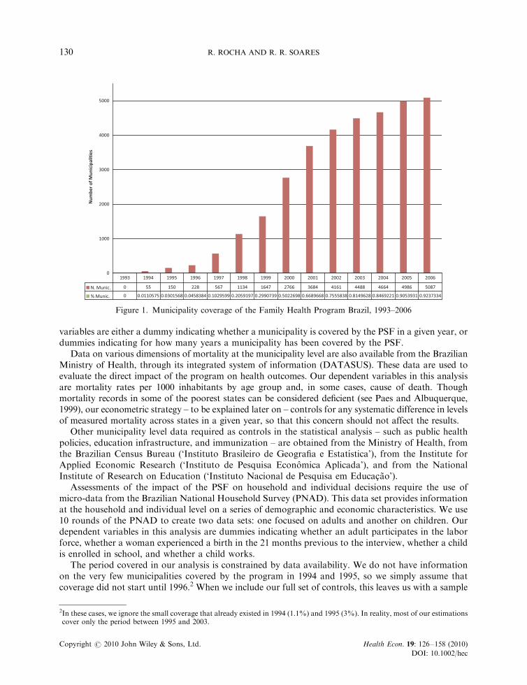
The history of growth of the program is portrayed in Figure 1. It was expanded from a minor pilotproject covering very few selected areas in 1994 to a nationwide large-scale intervention in 2006 (presentin more than 90% of municipalities and estimated to cover more than 85 million people; see BrazilianMinistry of Health, 2006b). The federal budget was concomitantly expanded, from R$ 280 million in1998 to R$ 2679 million in 2005 (or from US$ 233 million to US$ 1175 million). The acceleratedexpansion of the PSF starting in 1998 was a result of an explicit effort on the part of the centralgovernment, associated with the intensification of federal support and the development of a morestandardized ‘package.’

The federal nature of the program and the goal of the central government to expand it to virtually theentire country are, from an empirical perspective, convenient features of the Brazilian experience.Almost every municipality was eventually incorporated into the PSF, so adhesion to the program doesseem to have an exogenous dimension of variation. Still, as will be clear later on, the timing of adoptiondid depend on initial socioeconomic conditions, and this constitutes one of the main concerns in ourempirical analysis.

3. DATA

Data related to implementation of the program at the municipality level is available from the BrazilianMinistry of Health, through its Basic Attention Department (‘Departamento de Atenc- ao Basica’).These data provide the date of implementation in each municipality (starting from 1996). Our treatment



DOI: 10.1002/hec

variables are either a dummy indicating whether a municipality is covered by the PSF in a given year, ordummies indicating for how many years a municipality has been covered by the PSF.

Data on various dimensions of mortality at the municipality level are also available from the BrazilianMinistry of Health, through its integrated system of information (DATASUS). These data are used toevaluate the direct impact of the program on health outcomes. Our dependent variables in this analysisare mortality rates per 1000 inhabitants by age group and, in some cases, cause of death. Thoughmortality records in some of the poorest states can be considered deficient (see Paes and Albuquerque,1999), our econometric strategy – to be explained later on – controls for any systematic difference in levelsof measured mortality across states in a given year, so that this concern should not affect the results.

Other municipality level data required as controls in the statistical analysis – such as public healthpolicies, education infrastructure, and immunization – are obtained from the Ministry of Health, fromthe Brazilian Census Bureau (‘Instituto Brasileiro de Geografia e Estatıstica’), from the Institute forApplied Economic Research (‘Instituto de Pesquisa Economica Aplicada’), and from the NationalInstitute of Research on Education (‘Instituto Nacional de Pesquisa em Educac- ao’).

Assessments of the impact of the PSF on household and individual decisions require the use ofmicro-data from the Brazilian National Household Survey (PNAD). This data set provides informationat the household and individual level on a series of demographic and economic characteristics. We use10 rounds of the PNAD to create two data sets: one focused on adults and another on children. Ourdependent variables in this analysis are dummies indicating whether an adult participates in the laborforce, whether a woman experienced a birth in the 21 months previous to the interview, whether a childis enrolled in school, and whether a child works.

The period covered in our analysis is constrained by data availability. We do not have informationon the very few municipalities covered by the program in 1994 and 1995, so we simply assume thatcoverage did not start until 1996.2 When we include our full set of controls, this leaves us with a sample

Figure 1. Municipality coverage of the Family Health Program Brazil, 1993–2006

2In these cases, we ignore the small coverage that already existed in 1994 (1.1%) and 1995 (3%). In reality, most of our estimationscover only the period between 1995 and 2003.



DOI: 10.1002/hec

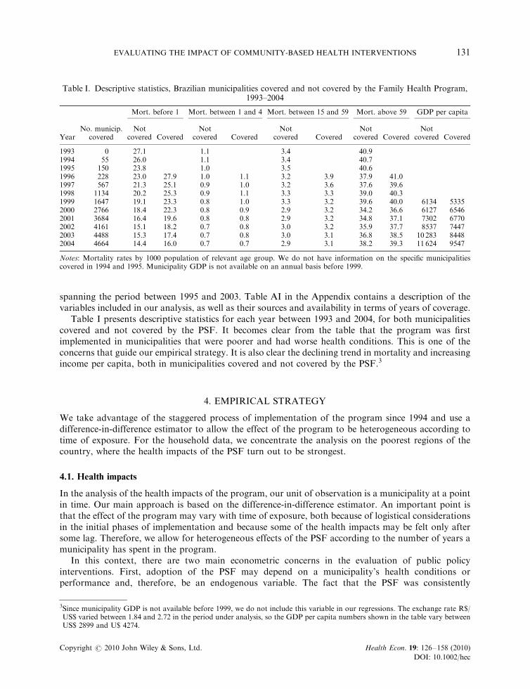
spanning the period between 1995 and 2003. Table AI in the Appendix contains a description of thevariables included in our analysis, as well as their sources and availability in terms of years of coverage.

Table I presents descriptive statistics for each year between 1993 and 2004, for both municipalitiescovered and not covered by the PSF. It becomes clear from the table that the program was firstimplemented in municipalities that were poorer and had worse health conditions. This is one of theconcerns that guide our empirical strategy. It is also clear the declining trend in mortality and increasingincome per capita, both in municipalities covered and not covered by the PSF.3

4. EMPIRICAL STRATEGY

We take advantage of the staggered process of implementation of the program since 1994 and use adifference-in-difference estimator to allow the effect of the program to be heterogeneous according totime of exposure. For the household data, we concentrate the analysis on the poorest regions of thecountry, where the health impacts of the PSF turn out to be strongest.

4.1. Health impacts

In the analysis of the health impacts of the program, our unit of observation is a municipality at a pointin time. Our main approach is based on the difference-in-difference estimator. An important point isthat the effect of the program may vary with time of exposure, both because of logistical considerationsin the initial phases of implementation and because some of the health impacts may be felt only aftersome lag. Therefore, we allow for heterogeneous effects of the PSF according to the number of years amunicipality has spent in the program.

In this context, there are two main econometric concerns in the evaluation of public policyinterventions. First, adoption of the PSF may depend on a municipality’s health conditions orperformance and, therefore, be an endogenous variable. The fact that the PSF was consistently

Table I. Descriptive statistics, Brazilian municipalities covered and not covered by the Family Health Program,1993–2004

Mort. before 1 Mort. between 1 and 4 Mort. between 15 and 59 Mort. above 59 GDP per capita

YearNo. municip.

coveredNot

covered CoveredNot

covered CoveredNot

covered CoveredNot

covered CoveredNot

covered Covered

1993 0 27.1 1.1 3.4 40.91994 55 26.0 1.1 3.4 40.71995 150 23.8 1.0 3.5 40.61996 228 23.0 27.9 1.0 1.1 3.2 3.9 37.9 41.01997 567 21.3 25.1 0.9 1.0 3.2 3.6 37.6 39.61998 1134 20.2 25.3 0.9 1.1 3.3 3.3 39.0 40.31999 1647 19.1 23.3 0.8 1.0 3.3 3.2 39.6 40.0 6134 53352000 2766 18.4 22.3 0.8 0.9 2.9 3.2 34.2 36.6 6127 65462001 3684 16.4 19.6 0.8 0.8 2.9 3.2 34.8 37.1 7302 67702002 4161 15.1 18.2 0.7 0.8 3.0 3.2 35.9 37.7 8537 74472003 4488 15.3 17.4 0.7 0.8 3.0 3.1 36.8 38.5 10 283 84482004 4664 14.4 16.0 0.7 0.7 2.9 3.1 38.2 39.3 11 624 9547

Notes: Mortality rates by 1000 population of relevant age group. We do not have information on the specific municipalitiescovered in 1994 and 1995. Municipality GDP is not available on an annual basis before 1999.

3Since municipality GDP is not available before 1999, we do not include this variable in our regressions. The exchange rate R$/US$ varied between 1.84 and 2.72 in the period under analysis, so the GDP per capita numbers shown in the table vary betweenUS$ 2899 and U$ 4274.



DOI: 10.1002/hec

expanded as part of an explicit effort of the central government, until it included almost allmunicipalities in Brazil, suggests that eventual adoption did not suffer so much from this endogeneityproblem. Still, endogeneity may be a serious concern in relation to the specific timing of adoption in agiven municipality. As long as adoption is correlated with some pre-existing condition, the municipalityfixed-effects present in a difference-in-difference approach take care of the problem. More worrisomeare the following possibilities: the timing of adoption is related to some dynamic characteristic of thedependent variable, such as when municipalities subject to particularly negative health shocks are morelikely to receive the program; or initial conditions are associated with a specific dynamic evolution of thedependent variable, such as when there is tendency toward convergence, so that initially worse-offmunicipalities naturally catch up to better-off ones.

Owing to a large number of municipalities (almost 5000 in most specifications), computationallimitations and reduced degrees of freedom prevent us from using municipality-specific linear trends.Therefore, our specification includes state-specific time dummies to deal to some degree with this issue.4

To the extent that differential dynamic behavior in mortality reflects differences across various areas ofthe country, this will be captured by different state-specific non-linear trends (time dummies). Still, thesepossibilities constitute our main concern in the empirical analysis, and we develop various procedures tocheck the robustness of our results to them. As an initial assessment of how serious these problems maybe, at the end of this section we follow Galiani et al. (2005) and conduct a hazard estimation of thedeterminants of the probability that a given municipality joins the program.

Our second concern is related to omitted variables. It is possible that good governments make use ofthe PSF and also implement various other social policies, in which case we may end up attributing to thePSF an effect that indeed comes from other actions taken by local governments. In order to account forthis possibility, we try to control for a wide range of municipality variables, encompassing differentdimensions of local policy that may be correlated with the implementation of the PSF and may also leadto improvements in health and reductions in mortality. With this goal in mind, our vector ofmunicipality controls includes the following dimensions: immunization coverage (BCG, measles, yellowfever, poliomyelitis and DTP, without the last two and with DT for adults),5 health infrastructure(number of beds and hospitals per capita), and education infrastructure (number of schools andteachers per capita).

Given the considerations above, our benchmark specification in this case is a difference-in-differenceallowing for heterogeneity in the effect of treatment according to time of exposure to the program, andalso allowing for state-specific year dummies. The main sources of variation used to identify the effectsof the program are: different timing of adoption across municipalities and different time of exposure. Soour basic empirical specification is the following:

Mortmt ¼ ah1XJj¼1

bhj :PSFjmt1gh:Xmt1Whm1mhst1emt; ð1Þ

where Mortmt denotes some age-specific mortality rate for municipality m in year t, PSFjmt indicates a

dummy variable assuming value 1 if municipality m in year t has been in the program for j years, Xmt

denotes a set of municipality level controls, Whm is a municipality fixed-effect, mhst is a state-specific year

4Note that this strategy also deals, to a great extent, with the measurement problem alluded to in the previous section. Anysystematic variation in mortality recording across states at a point in time, or across time within a state, is controlled for by thestate-year dummies. The only remaining potential bias due to measurement is related to a situation where recording issystematically improved by the presence by the PSF. But notice that in this case the bias would be in the direction of finding apositive effect of the program on mortality.

5It is possible that the PSF improves the delivery of immunization. Still, since widespread immunization in Brazil predates the PSF,we want to be able to estimate the effect of the program independently from its effects on immunization. Our qualitative resultsremain very similar when we exclude the immunization variables from the estimation.



DOI: 10.1002/hec

dummy (26 non-linear state-specific trends), emt is a random error term, and ah, bhj ’s, and gh areparameters.

Finally, in order to account for the fact that the variance of mortality is strongly related topopulation size, we weight the regressions by municipality population. Also, to account for thepossibility of serially correlated and heteroskedastic errors, and to avoid overestimation of thesignificance of estimated coefficients, we cluster standard errors at the municipality level (as suggestedby Bertrand et al., 2004).

4.2. Behavioral impacts

In the analysis of the impacts of the program on individual behavior, our unit of observation is anindividual within a municipality at a point in time. We restrict the analysis to regions where the healthimpacts of the program seem to have been strongest. For obvious reasons, these are also the placeswhere we would hope to find the clearest changes in behavior. In this case, our sample, extracted fromthe Brazilian National Household Survey, covers 361 municipalities (in the north and northeastregions). Given the reduced number of municipalities, we also allow for municipality-specific lineartrends. This has at least one great advantage in relation to the approach suggested for the case of thehealth impacts of the program: differential trends across municipalities are immediately controlled for,taking care of one of the main concerns in our previous discussion.

Since the outcomes of interest now are represented by dichotomous categorical variables (laborsupply, employment, school enrollment, and occurrence of a birth), we estimate probit models(all results are reported as marginal effects calculated at the mean of independent variables). Here again,the main sources of variation used to identify the effects of the program are: different timing ofadoption across municipalities and different time of exposure. So our basic specification is thefollowing:

PðBehaviorimt ¼ 1Þ ¼ F ab1XJj¼1

bbj � PSFjmt1jb � Zimt1gb � Xmt1Wbm1mbt 1rbm � t

!; ð2Þ

where Behaviorimt denotes some dichotomous discrete indicator for the behavior of individual i inmunicipality m and year t, PSFj

mt indicates a dummy variable assuming value 1 if municipality m in yeart has been in the program for j years, Zimt represents a set of individual level controls, Xmt denotes a setof municipality level controls, Wbm is a municipality fixed-effect, mbt is a year dummy, t represents a lineartime trend, F( � ) is the normal distribution function, and ab, bbj ’s, j

b, gb, and rbm’s are parameters.6

This specification greatly reduces concerns related to differential dynamic behavior of the dependentvariable across municipalities, as those expressed in the last subsection. Still, there remains thepossibility of omitted variables associated with other relevant dimensions of policy. In this respect, wefollow the same strategy outlined for the case of the municipality level analysis. We also cluster standarderrors at the municipality level, to account for the possibility of correlation of residuals withinmunicipalities (across individuals and time) and to avoid overestimation of the significance of estimatedcoefficients (as suggested by Bertrand et al., 2004 in an OLS context).

4.3. Determinants of adoption of the Family Health Program

As an initial assessment of the determinants of adoption of the PSF and of how serious the issue ofdynamic endogeneity may be, we follow Galiani et al. (2005). We conduct a hazard estimation of the

6It is known that fixed-effects estimates are not consistent in probit models, and that this may bias estimates of other parameters.But Fernandez-Val (2007) has recently shown that, in this setting, estimates of average marginal effects have negligible biasrelative to their true values (for a wide variety of distributions of regressors and individual effects). Since we concentrate ourdiscussion on marginal effects, we proceed with the fixed-effects probit estimation and trust on these results.



DOI: 10.1002/hec

probability that a given municipality joins the program. Specifically, our dependent variable is a dummyindicating the presence of the program in a municipality. As soon as municipalities join the program,they leave the sample. So we estimate the effect of municipalities’ characteristics on the probability ofjoining the program. Our main interest is on how this probability is related to fixed municipalitycharacteristics and to changes in endogenous variables or other policy dimensions. Therefore, ourhazard estimation evaluates the probability that a municipality joins the PSF as a function of shocks tohealth variables (changes in mortality in previous years), changes in other dimensions of public policy, aset of political variables indicating the party of the mayor,7 and a set of socioeconomic variables8

indicating the initial conditions of the municipality.Results of this estimation are presented in the Appendix Table AII. The first three columns consider,

respectively, the 1st, 2nd, and 3rd lags of mortality before age 1, each at time. The remaining threecolumns include mortality between ages 1 and 4 and between ages 15 and 59 in the analysis, againconsidering the 1st, 2nd, and 3rd lags separately.9

The results indicate that adoption of the program seems to be correlated with past health shocks, butthat the quantitative impacts are extremely small when compared to other variables. The estimatedcoefficients imply that even substantial mortality shocks lead only to modest increases in the probabilityof program adoption: a one standard deviation increase in lagged mortality before age 1 increases theprobability of program adoption by 3.5 percentage points (results are similar in the case of mortality indifferent age groups). In contrast, political considerations as well as initial municipality characteristicsare quantitatively very important. Municipalities governed by the main left wing parties – WorkersParty (PT), Popular Socialist Party (PPS), and Socialist Party (PSB) – and by the Social DemocratParty were more likely to adopt the program in any given year. The estimated coefficients imply that, ifthe mayor belonged to one of the parties mentioned before, the probability that a municipality wouldjoin the program in a given year would be increased by between 20 and 60 percentage points. Politicalconsiderations seem to be key in determining program implementation.

Also, several initial characteristics are correlated with early adoption. Overall, municipalities withinitially worse-off conditions were more likely to adopt the PSF. In terms of initial variables, highermortality before age 1, lower number of schools per capita, higher number of members per household,and lower income per capita were historically associated with early entry in the Family Health Program.Doubling household income per capita, for example, is associated with a 22 percentage point reductionin the probability that a municipality joins the program in a given year.10

In any case, adoption of the program is not greatly affected by shocks to health. So the dynamic issueof decision of adoption being driven by changes in dependent variables (health outcomes) does not seemto be serious enough to impair the use of the empirical strategy outlined above. In addition, the fact thatprogram implementation is greatly affected by political considerations seems to guarantee some degreeof exogeneity.

7During almost the entire period covered by the sample, the Social Democratic Party holds the Brazilian presidential office.Therefore, we do not include dummies indicating whether the mayor belongs to the party of the president, and choose to controlonly for the identity of the party.

8The initial conditions include initial values of: health variables (mortality before 1, between 1 and 4, between 15 and 59, and above60), public policy variables (hospitals, hospital beds, schools, and teachers), average schooling, average age of the head of thehousehold, average number of members in a household, percentage of households in vulnerable socioeconomic conditions (fouror more members per working member and head of the household with less than 4 years of schooling), average household incomeper capita (ln), and unemployment rate.

9We do not include mortality above age 59 in this analysis because, as will be seen later on, it is not significantly affected by theprogram. In addition, the cross-municipality variance in old age mortality is relatively small when compared to its mean.

10An interesting aspect suggested by the table is that there seems to be some substitutability across different policy alternatives:municipalities more likely to adopt the PSF are those that have not increased the number of hospitals or the number of schools inrecent years.



DOI: 10.1002/hec

5. IMPACT ON MORTALITY

5.1. Main results

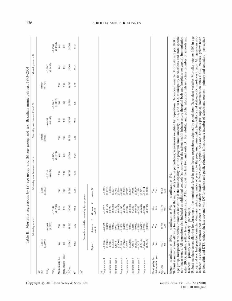
Table II presents some preliminary results from a simpler specification, where we still do not allow forheterogeneity in response according to time of exposure to the program. The table presents results fromthree regressions for each of the four different age groups – before age 1, from age 1 to 4, from age 15 to59, and above age 59. In the first regression, the treatment is defined as a municipality being covered bythe program, while in the second and third regressions, treatment is defined, respectively, as amunicipality having been covered for at least one or two years (first and second lags of programimplementation). The results show that program implementation takes some time to manifest itself onmortality and, in addition, its impact seems to change considerably through time. This evidence justifiesthe use of our benchmark specification, where we allow for heterogeneity according to time of exposure.

Table II presents the results from our baseline specification. The four columns display the estimatedcoefficients of the effects of the PSF on mortality for the four different age groups. The table suggests astrong negative correlation between program exposure and mortality for all age groups below 59, andsome mild negative correlation for the age group above 59. Quantitative impacts are particularly strongfor mortality before age 1, but in relative terms the impacts are also substantial for other age groups.For example, the estimated coefficients imply that municipalities that have been in the program forthree years reduce infant mortality by 1.8 per 1000 more than otherwise identical municipalities not inthe program. Taking the 1993 average infant mortality for Brazil (27 per 1000), this corresponds to a6.7% reduction in the mortality rate. For a municipality 8 years into the program, there is a reduction of5.4 per 1000, corresponding to 20% of the 1993 average.

For mortality rate between ages 1 and 4, the coefficients correspond to reductions of 6.4% (0.07 inabsolute terms) for municipalities 3 years into the program, and 24% (0.26 in absolute terms) formunicipalities 8 years into the program. Analogous numbers for mortality between ages 15 and 59 are3.2% (0.11 in absolute terms) for 3 years into the program and 11.2% (0.38 in absolute terms) for 8years into the program.

The effect of the PSF on mortality above age 59 is much less robust in terms of significance and lessimportant in terms of magnitude. The impacts implied by the point estimates are quite small ascompared to the average mortality observed in the age group. So municipalities 3 years into theprogram are estimated to experience additional reductions in mortality of 0.56 per 1000. Takingthe 1993 mortality rate as a reference point, this represents a reduction of only 1.4% in mortality. Theanalogous number for 8 years into the program is 1.21 per 1000, corresponding to only 2.9% of the 1993national average.

The time span covered by our sample allows us to look only at municipalities that have been in theprogram for 8 years or less. Within this time frame, mortality reductions seem to generally increase witheach additional year of program exposure. So, for mortality before age 1, there is an average reductionin mortality of 0.69 per additional year in the PSF, while the analogous number for mortality betweenages 1 and 4 and 15 and 59 is roughly 0.035.11

5.2. Heterogeneity in response

In order to better understand how the Family Health Program actually worked, its strengths andweaknesses, we explore some dimensions of potential heterogeneity in response. Heterogeneity in

11This result is not due to municipality heterogeneity correlated with time of exposure to the program. In the Appendix TableA.III, we interact the treatment dummies of Program Year 3, Program Year 4, and Program Year 5 with dummies indicating‘early movers’ (municipalities that joined the PSF during the first 3 years). The results remain unchanged, and the interactions oftreatment dummies with ‘early movers’ are not statistically significant. So the larger effect for municipalities that have been in theprogram for a long time is not related to some unobserved characteristic of these ‘early movers.’



DOI: 10.1002/hec

TableII.Mortality

regressionsby(a)agegroupand(b)agegroupandsex,Brazilianmunicipalities,1993–2004

Mortality

rate

o1

Mortality

rate

between1and4

Mortality

rate

between15and59

Mortality

rate

459

(a)a

PSF

�0.1115

�0.0164

�0.0256

0.0364

(0.2691)

(0.0132)

(0.0165)

(0.1704)

PSFt-1

�0.5908��

�0.0284��

�0.0483��

�0.2967��

(0.2752)

(0.0134)

(0.0143)

(0.1437)

PSFt-2

�1.3149��

�0.0434��

�0.0462��

�0.4306��

(0.3909)

(0.0178)

(0.0172)

(0.1560)

Municipality

f.e.

Yes

Yes

Yes

Yes

Yes

Yes

Yes

Yes

Yes

Yes

Yes

Yes

State-specific

year

f.e.

Yes

Yes

Yes

Yes

Yes

Yes

Yes

Yes

Yes

Yes

Yes

Yes

NObs

38762

38762

38762

38769

38769

38769

38769

38769

38769

38769

38769

38769

R2

0.62

0.62

0.62

0.36

0.36

0.36

0.81

0.81

0.81

0.75

0.75

0.75

(b)b

Dependentvariable:mortality

byagegroup

Before

1Between

1and4

Between

15

and59

Above

59

(b)

Program

year1

�0.5690��

�0.0322��

�0.0397��

�0.0713

(0.2701)

(0.0156)

(0.0165)

(0.1832)

Program

year2

�0.7614��

�0.0494��

�0.0790��

�0.2396

(0.3386)

(0.0172)

(0.0200)

(0.2234)

Program

year3

�1.8144��

�0.0707��

�0.1142��

�0.5590��

(0.4706)

(0.0231)

(0.0252)

(0.2544)

Program

year4

�2.6899��

�0.1159��

�0.1595��

�0.8310��

(0.6706)

(0.0279)

(0.0323)

(0.3802)

Program

year5

�3.6592��

�0.1626��

�0.1989��

�0.9035��

(0.8202)

(0.0373)

(0.0407)

(0.3917)

Program

year6

�4.5655��

�0.2158��

�0.2642��

�1.0685��

(1.1021)

(0.0432)

(0.0470)

(0.4926)

Program

year7

�4.0427��

�0.2160��

�0.2882��

�1.2634��

(1.2616)

(0.0515)

(0.0631)

(0.5871)

Program

year8

�5.4048��

�0.2560��

�0.3834��

�1.2114�

(1.5642)

(0.0562)

(0.0702)

(0.7170)

Municipality

f.e.

Yes

Yes

Yes

Yes

State-specific

year

f.e.

Yes

Yes

Yes

Yes

No.Obs

46771

46778

46778

46778

R2

0.61

0.34

0.81

0.75

Notes:�significantat10%

;��

significantat5%

;��significantat1%

.aRobuststandard

errors

allowingforclusteringatthemunicipality

levelin

parentheses;regressionsweightedbypopulation.Dependentvariable:Mortality

rate

per

1000in

agegroup.Independentvariables:dummiesindicatingifthemunicipality

isin

theprogram

simultaneously,in

t-1,andin

t-2,municipality

fixed-effects

andstate-specific

non-lineartrends.Allregressionsalsoincluded

asadditionalcontrols(notshownin

thetable):healthinfrastructure

(hospitalbedsandhospitalsper

capita),im

munization

rates(BCG,measles,yellow

fever,poliomyelitis

andDTP,withoutthelast

twoandwithDT

foradults),andpubliceducationinfrastructure

(number

ofschools

and

teachers–primary

andsecondary

–per

capita).

bRobust

stan

darderrors

allowingforclusteringat

themunicipalitylevelin

parentheses;regressionsweigh

tedbypopulation.Dependentvariab

le:Mortalityrate

per

1000

inage

groupan

dsex.

Independentvariab

les:dummiesindicatingnumber

ofyearsinto

theprogram

,municipalityfixed-effects

andstate-specificnon-lineartrends.Allregressionsalso

included

asad

ditional

controls

(notshown

inthetable):

health

infrastructure

(hospital

bedsan

dhospitalsper

capita),im

munization

rates(BCG,measles,yellow

fever,

poliomyelitisan

dDTP,withoutthelasttw

oan

dwithDTforad

ults),an

dpubliceducationinfrastructure

(number

ofschoolsan

dteachers–primaryan

dsecondary–per

capita).



DOI: 10.1002/hec

response may be related to, among other things, initial conditions, geographic characteristics, or specificcauses of death. In this subsection, we explore the differential impact of the program along some ofthese dimensions.

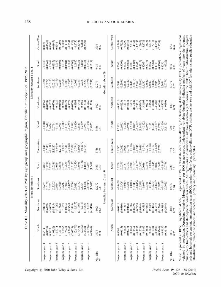
5.2.1. Regions. Table III presents results from regressions identical to those from Table II, but ranseparately for each of the five geographic regions of Brazil: south, southeast, center-west, northeast, andnorth. The results reveal a clear pattern: the two poorest regions, which are also those with lowerprovision of several public goods – the north and the northeast – are by far the ones enjoying thegreatest benefits from the program.12 In the north, a municipality 8 years into the program is estimatedto experience a reduction of 15.0 per 1000 in infant mortality rate, while the analogous reduction for theNortheast is 13.8 per 1000. The impact of the program for these two regions appears as significant andlarge in magnitude for all age groups analyzed, including mortality above 59.In other regions, there is some evidence on the significant impacts of the PSF on mortality between 1and 4 and 15 and 59 in the southeast, between 15 and 59 and above 59 in the center-west, and between 1and 4 in the south, but results are never as robust as for the north and northeast.

The regional heterogeneity in response to the program is also consistent with results (not shown here)indicating that municipalities with lower levels of urbanization, less access to treated water, and lesscoverage from the public sewerage system benefited particularly from program implementation (see theworking paper version of this paper – Rocha and Soares, 2009 – for these results). Overall, municipalitieswith initially worse socioeconomic conditions seem to have been the greatest beneficiaries of the PSF.

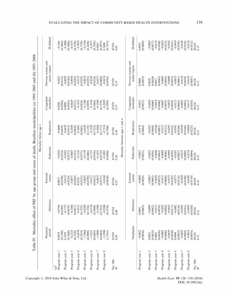
5.2.2. Cause of death. In order to shed further light on the driving forces behind the impacts of theFamily Health Program, Table IV decompose the effect of the PSF on mortality by cause of death.Each table presents the same specification from Table II for a particular age group, for mortalitydecomposed by the main causes of death within that age group. The causes of death considered for eachage group are enumerated in the table itself (see Appendix Table AIV for a detailed description of thespecific causes of death included in each group).13

For mortality before 1, Table IV shows significant impacts of the program mainly on perinatal periodconditions, infectious diseases, endocrine diseases, and respiratory diseases. Most of these estimatedeffects are in line with what should be expected from the type of intervention implied by the program.The estimated effect on ill-defined conditions during the first years of implementation, which may seemstrange at first sight, is probably due to the fact that presence of the PSF is associated with a reductionin the number of deaths without proper diagnosis (reduction in the measurement error in cause ofdeath).14 Quantitatively, the largest impacts of the program on this age group are associated withmortality due to perinatal period conditions, infectious diseases, and respiratory diseases. These threecauses of death include, for example, problems associated with complications during pregnancy,diarrhea and other intestinal diseases, influenza, asthma, and bronchitis. These are precisely conditionsagainst which the kind of support and information provided by the presence of the Family Health

12For example, in the beginning of the period under analysis (1993), income per capita was R$2810 in the northeast and R$4630 inthe north, against a national average for Brazil of R$6280 (values in R$ of 2000, from www.ipeadata.gov.br).

13We also experimented with morbidity data based on hospital admissions by place of residence, but found no significant impact ofthe program on any age group or disease. It is not clear whether this is due to reporting error in the data, or to the fact that thePSF may facilitate hospital access for certain fractions of the population. Given that most of health problems do not culminatein death, one should expect the impact of the Family Health Program on general health to be stronger than the impact onmortality estimated here.

14Notice that this interpretation is consistent with the fact that the effect on ill-defined conditions is reduced in magnitude andceases to be significant after year 6. Also, this interpretation means that a fraction of the deaths that before were registered as dueto ill-defined conditions are now properly classified into some other cause of death. This would imply an artificial increase in thenumber of deaths attributable to the causes, which in turn would tend to minimize the estimated impact of the program on theseother causes of death. So, if anything, our estimates on other causes of death are likely to be slightly biased toward zero.



DOI: 10.1002/hec

TableIII.

Mortality

effect

ofPSF

byagegroupandgeographic

region,Brazilianmunicipalities,1995–2003

Mortality

before

1Mortality

between1and4

North

Northeast

Southeast

South

Center-West

North

Northeast

Southeast

South

Center-West

Program

year1

0.6614

�2.0970��

0.1669

0.4802

�0.0461

�0.0010

�0.0567�

�0.0218

�0.0280

0.0128

(0.8555)

(0.6069)

(0.3159)

(0.4210)

(0.5543)

(0.0618)

(0.0328)

(0.0179)

(0.0368)

(0.0645)

Program

year2

0.3423

�3.0674��

0.5253

0.7267

�1.1315

0.0636

�0.1225��

�0.0155

�0.0668�

0.0606

(1.0352)

(0.8445)

(0.3205)

(0.5386)

(1.1217)

(0.0764)

(0.0370)

(0.0211)

(0.0387)

(0.0847)

Program

year3

�2.7711��

�5.1062��

0.1644

0.4099

�1.9049

�0.1151

�0.1620��

�0.0190

�0.0590

0.0341

(1.3771)

(1.1782)

(0.4619)

(0.5876)

(1.7159)

(0.0971)

(0.0496)

(0.0288)

(0.0405)

(0.1207)

Program

year4

�5.3465��

�7.1291��

0.2656

0.2739

�1.8297

�0.2012�

�0.2484��

�0.0534�

�0.0175

�0.0044

(1.7341)

(1.8925)

(0.5897)

(0.7630)

(2.3510)

(0.1123)

(0.0727)

(0.0280)

(0.0504)

(0.1418)

Program

year5

�8.7942��

�8.3549��

�0.0207

�0.1699

�4.8848

�0.4263��

�0.3378��

�0.0307

�0.0802

�0.0341

(2.6323)

(2.3365)

(0.7784)

(0.7137)

(3.2330)

(0.1591)

(0.0970)

(0.0370)

(0.0500)

(0.1920)

Program

year6

�12.6763��

�10.9172��

0.0482

�0.2554

�5.7943�

�0.6450��

�0.4393��

�0.0641�

�0.0947

�0.1750

(3.7045)

(3.1196)

(0.9172)

(0.8955)

(3.1028)

(0.1811)

(0.1048)

(0.0387)

(0.0627)

(0.2244)

Program

year7

�12.7825��

�10.9113��

0.5394

�0.3188

�10.2979��

�0.2939

�0.4862��

�0.0331

�0.1026

�0.2881

(5.4328)

(3.7662)

(1.1476)

(1.1068)

(4.2799)

(0.2903)

(0.1334)

(0.0527)

(0.0733)

(0.2820)

Program

year8

�14.9974��

�13.8228��

�0.7853

0.7429

�0.3850

�0.5465��

�0.0720

�0.2562��

(4.9848)

(4.5430)

(1.3497)

(1.6491)

(0.4827)

(0.1333)

(0.0737)

(0.1219)

No.Obs

3436

14021

12272

9439

3756

3436

14021

12279

9439

3756

R2

0.71

0.63

0.61

0.45

0.49

0.41

0.40

0.27

0.20

0.32

Mortality

between15and59

Mortality

above59

North

Northeast

Southeast

South

Center-West

North

Northeast

Southeast

South

Center-West

Program

year1

0.0601

�0.0911��

�0.0138

0.0209

0.0287

1.2565�

�0.5510

0.0991

0.2266

�0.3658

(0.0615)

(0.0386)

(0.0306)

(0.0290)

(0.0615)

(0.6695)

(0.4133)

(0.2096)

(0.3004)

(0.7128)

Program

year2

�0.0528

�0.1557��

�0.0434

0.0157

0.0026

�0.2253

�1.2913��

0.1821

0.4922

�0.7290

(0.0937)

(0.0452)

(0.0265)

(0.0307)

(0.0785)

(0.8936)

(0.4653)

(0.2729)

(0.3469)

(0.8341)

Program

year3

�0.1464

�0.1866��

�0.0843��

0.0210

�0.1846�

�1.5530

�1.6477��

0.0646

0.6008

�2.3149

(0.1155)

(0.0599)

(0.0343)

(0.0355)

(0.1009)

(1.1085)

(0.5563)

(0.2618)

(0.3802)

(1.4058)

Program

year4

�0.3032��

�0.2920��

�0.0854��

�0.0152

�0.2421

�2.4192��

�2.9310��

0.2569

0.9042��

�3.5137��

(0.1328)

(0.0944)

(0.0390)

(0.0473)

(0.1616)

(1.1451)

(0.9767)

(0.2866)

(0.4317)

(1.2847)

Program

year5

�0.4467��

�0.3385��

�0.0947�

0.0086

�0.3748�

�4.3822��

�3.1603��

0.4530

0.3205

�3.6781��

(0.1588)

(0.1088)

(0.0565)

(0.0571)

(0.2132)

(1.3944)

(1.0131)

(0.3642)

(0.5019)

(1.5535)

Program

year6

�0.6123��

�0.4003��

�0.1453��

�0.0206

�0.5198��

�4.7981��

�3.2521��

0.5509

0.6669

�6.7375��

(0.1738)

(0.1445)

(0.0662)

(0.0645)

(0.2102)

(1.9348)

(1.3140)

(0.4109)

(0.7781)

(1.7915)

Program

year7

�0.9682��

�0.5037��

�0.0577

0.0816

�0.6049��

�4.8187

�4.5100��

1.2906�

0.4730

�4.7583�

(0.3246)

(0.1784)

(0.0822)

(0.0630)

(0.2720)

(3.9731)

(1.6616)

(0.6685)

(0.9301)

(2.5538)

Program

year8

�0.9655��

�0.5898��

�0.1188

�0.0188

�5.3666

�4.9774��

1.2654

0.8350

(0.3114)

(0.2044)

(0.0925)

(0.0786)

(4.1192)

(1.9199)

(0.9774)

(1.0922)

No.Obs

3436

14021

12279

9439

3756

3436

14021

12279

9439

3756

R2

0.75

0.77

0.80

0.61

0.52

0.79

0.71

0.67

0.50

0.64

Notes:� significantat10%;��

significantat5%

;�� significantat1%

.Robust

standard

errors


level

inparentheses;regressions

weighted

bypopulation.Dependentvariable:Mortality

rate

per

1000in

agegroup.Independentvariables:

dummiesindicatingnumber

ofyears

into

theprogram,

municipality

fixed-effects

andstate-specificnon-lineartrends.Allregressionsalsoincluded



(hospital

bedsandhospitalsper

capita),im

munizationrates(BCG,measles,yellowfever,poliomyelitisandDTP,withoutthelasttw

oandwithDTforadults),andpubliceducation

infrastructure

(number

ofschoolsandteachers–primary

andsecondary

–per

capita).



DOI: 10.1002/hec

TableIV

.Mortality

effect

ofPSF

byagegroupandcause

ofdeath,Brazilianmunicipalities

(a)1995–2003and(b)1993–2004

Mortality

before

age1

Perinatal

period

Infectious

External

causes

Endocrine

Respiratory

Congenital

anomalies

Nervoussystem

and

sensesorgans

Ill-defined

(a)a

Program

year1

0.0879

�0.0784

0.0033

�0.0292

�0.0448

0.0280

�0.0267�

�0.1661�

(0.1590)

(0.0589)

(0.0190)

(0.0224)

(0.0479)

(0.0502)

(0.0152)

(0.1002)

Program

year2

0.1859

�0.1752��

�0.0123

�0.0292

�0.0470

0.0098

�0.0058

�0.3006��

(0.1868)

(0.0638)

(0.0210)

(0.0275)

(0.0512)

(0.0581)

(0.0186)

(0.1006)

Program

year3

�0.2225

�0.3464��

�0.0071

�0.0607�

�0.2050��

�0.0629

�0.0050

�0.5357��

(0.2520)

(0.0917)

(0.0265)

(0.0333)

(0.0628)

(0.0727)

(0.0202)

(0.1526)

Program

year4

�0.6870�

�0.4511��

0.0156

�0.1216��

�0.2601��

�0.1625�

�0.0152

�0.5055��

(0.3818)

(0.1222)

(0.0331)

(0.0371)

(0.0841)

(0.0838)

(0.0259)

(0.1798)

Program

year5

�1.2964��

�0.4589��

�0.0021

�0.1159��

�0.4238��

�0.1580�

�0.0074

�0.5556��

(0.4909)

(0.1556)

(0.0398)

(0.0468)

(0.1139)

(0.0899)

(0.0293)

(0.2428)

Program

year6

�1.8221��

�0.6734��

�0.0127

�0.1757��

�0.5320��

�0.1934�

�0.0539�

�0.5871�

(0.6603)

(0.2000)

(0.0412)

(0.0536)

(0.1522)

(0.1066)

(0.0324)

(0.3285)

Program

year7

�1.9880��

�0.5590��

�0.0053

�0.1853��

�0.4504��

�0.3309��

�0.0573

0.0467

(0.8464)

(0.2762)

(0.0571)

(0.0718)

(0.1777)

(0.1578)

(0.0406)

(0.4937)

Program

year8

�3.3990��

�0.9300��

�0.0160

�0.3091��

�0.7318��

�0.2039

�0.0674

0.5490

(1.2161)

(0.3370)

(0.0650)

(0.0960)

(0.1996)

(0.1889)

(0.0545)

(0.7473)

No.Obs

42924

42924

42924

42924

42924

42924

42924

42924

R2

0.58

0.46

0.25

0.28

0.36

0.37

0.18

0.61

Mortality

betweenages

1and4

Neoplasm

sInfectious

External

causes

Endocrine

Respiratory

Congenital

anomalies

Nervoussystem

and

sensesorgans

Ill-defined

Program

year1

�0.0022

0.0001

�0.0088

�0.0021

�0.0178��

�0.0012

0.0004

0.0035

(0.0030)

(0.0063)

(0.0059)

(0.0031)

(0.0064)

(0.0032)

(0.0032)

(0.0069)

Program

year2

0.0021

�0.0089

�0.0067

�0.0055

�0.0165��

�0.0024

0.0029

�0.0082

(0.0035)

(0.0062)

(0.0065)

(0.0036)

(0.0068)

(0.0040)

(0.0034)

(0.0077)

Program

year3

0.0005

�0.0213��

�0.0059

�0.0048

�0.0146�

�0.0014

0.0017

�0.0132

(0.0036)

(0.0076)

(0.0075)

(0.0043)

(0.0087)

(0.0046)

(0.0043)

(0.0104)

Program

year4

�0.0001

�0.0282��

�0.0212��

�0.0088�

�0.0215�

�0.0047

�0.0003

�0.0203�

(0.0040)

(0.0088)

(0.0088)

(0.0048)

(0.0113)

(0.0053)

(0.0045)

(0.0123)

Program

year5

�0.0029

�0.0455��

�0.0253��

�0.0094

�0.0295��

�0.0032

�0.0080

�0.0242

(0.0050)

(0.0113)

(0.0103)

(0.0058)

(0.0142)

(0.0056)

(0.0053)

(0.0161)

Program

year6

0.0009

�0.0402��

�0.0375��

�0.0201��

�0.0391��

�0.0111�

�0.0033

�0.0419��

(0.0055)

(0.0126)

(0.0116)

(0.0067)

(0.0160)

(0.0063)

(0.0061)

(0.0198)

Program

year7

�0.0055

�0.0505��

�0.0304��

�0.0235��

�0.0550��

�0.0083

�0.0124�

�0.0168

(0.0069)

(0.0161)

(0.0140)

(0.0080)

(0.0186)

(0.0082)

(0.0070)

(0.0256)

Program

year8

�0.0016

�0.0692��

�0.0396��

�0.0219��

�0.0684��

�0.0117

�0.0143�

�0.0126

(0.0076)

(0.0188)

(0.0170)

(0.0094)

(0.0225)

(0.0103)

(0.0087)

(0.0312)

No.Obs

48636

48636

48636

48636

48636

48636

48636

48636

R2

0.13

0.21

0.18

0.19

0.21

0.15

0.15

0.37



DOI: 10.1002/hec

Mortality

betweenages

15and59

Neoplasm

sExternalcauses

Endocrine

Respiratory

Circulatory

Digestive

Ill-defined

(b)b

Program

year1

0.0042

�0.0007

�0.0124��

�0.0001

�0.0140��

0.0006

�0.0015

(0.0031)

(0.0075)

(0.0037)

(0.0028)

(0.0047)

(0.0028)

(0.0056)

Program

year2

0.0029

�0.0088

�0.0161��

�0.0051�

�0.0156��

�0.0038

�0.0095

(0.0038)

(0.0102)

(0.0045)

(0.0027)

(0.0057)

(0.0031)

(0.0074)

Program

year3

0.0078�

�0.0241��

�0.0224��

�0.0070��

�0.0216��

�0.0058

�0.0175��

(0.0045)

(0.0120)

(0.0059)

(0.0033)

(0.0066)

(0.0036)

(0.0086)

Program

year4

0.0075

�0.0383��

�0.0276��

�0.0093��

�0.0200��

�0.0082�

�0.0316��

(0.0054)

(0.0149)

(0.0072)

(0.0040)

(0.0085)

(0.0043)

(0.0111)

Program

year5

0.0073

�0.0474��

�0.0352��

�0.0089�

�0.0196�

�0.0092�

�0.0314��

(0.0065)

(0.0210)

(0.0089)

(0.0051)

(0.0100)

(0.0056)

(0.0145)

Program

year6

0.0048

�0.0637��

�0.0437��

�0.0139��

�0.0275��

�0.0111�

�0.0413��

(0.0081)

(0.0271)

(0.0103)

(0.0066)

(0.0132)

(0.0064)

(0.0207)

Program

year7

0.0216�

�0.0669��

�0.0511��

�0.0137�

�0.0196

�0.0237��

�0.0493��

(0.0122)

(0.0335)

(0.0128)

(0.0077)

(0.0203)

(0.0093)

(0.0244)

Program

year8

0.0049

�0.1129��

�0.0492��

�0.0312��

�0.0059

�0.0254��

�0.0311

(0.0141)

(0.0402)

(0.0135)

(0.0100)

(0.0233)

(0.0121)

(0.0311)

No.Obs

42931

42931

42931

42931

42931

42931

42931

R2

0.67

0.77

0.58

0.54

0.70

0.48

0.68

Mortality

aboveage59

Neoplasm

sExternalcauses

Endocrine

Respiratory

Circulatory

Ill-defined

Program

year1

�0.0013

0.0095

�0.0102

0.0476

�0.0776

0.0952

(0.0337)

(0.0150)

(0.0249)

(0.0465)

(0.0837)

(0.0854)

Program

year2

0.0756�

�0.0130

0.0186

0.0311

�0.0925

�0.0876

(0.0446)

(0.0178)

(0.0318)

(0.0511)

(0.1019)

(0.1088)

Program

year3

0.0820�

�0.0024

�0.0088

�0.0271

�0.1237

�0.2815�

(0.0465)

(0.0184)

(0.0400)

(0.0549)

(0.1335)

(0.1441)

Program

year4

0.0878

�0.0128

�0.0494

0.0166

�0.2309

�0.4816��

(0.0575)

(0.0214)

(0.0511)

(0.0647)

(0.1781)

(0.1906)

Program

year5

0.0659

�0.0188

�0.0801

�0.0397

�0.2766

�0.3693�

(0.0698)

(0.0278)

(0.0582)

(0.0838)

(0.2014)

(0.2234)

Program

year6

0.1590�

�0.0381

�0.0417

0.0493

�0.3051

�0.5848�

(0.0910)

(0.0299)

(0.0720)

(0.1132)

(0.2987)

(0.2991)

Program

year7

0.1077

�0.0193

�0.0438

0.0124

�0.4783

�0.4993

(0.1223)

(0.0404)

(0.0893)

(0.1514)

(0.4795)

(0.3977)

Program

year8

0.1550

�0.0581

�0.1799

�0.0929

�0.7436

�0.1479

(0.1643)

(0.0464)

(0.1105)

(0.1800)

(0.6622)

(0.5698)

No.Obs

42931

42931

42931

42931

42931

42931

R2

0.82

0.35

0.64

0.76

0.82

0.79

Notes:� significantat10%

;��

significantat5%


.aRobust

standard

errors

allowingforclusteringatthemunicipalitylevel

inparentheses;regressionsweightedbypopulation.Dependentvariab

le:Mortalityrate

per

1000in

agegroup.Independent

variables:dummiesindicatingnumber

ofyears

into

theprogram,municipalityfixed-effects



the

table):healthinfrastructure


capita),im

munizationrates(BCG,measles,yellowfever,poliomyelitisan

dDTP,withoutthelasttw

oandwithDTforadults),andpublic

educationinfrastructure

(number


andsecondary

–per

capita).

bRobust

stan

dard

errors


level

inparentheses;regressionsweigh

tedbypopulation.Dependentvariable:Mortality

rate

per

1000in

agegroup.Independent

variables:dummiesindicatingnumber

ofyears

into

theprogram,municipality

fixed-effects



the

table):healthinfrastructure


capita),im

munizationrates(BCG,measles,yellow

fever,poliomyelitisandDTP,withoutthelasttw

oandwithDTforadults),andpublic

educationinfrastructure

(number


andsecondary–per

capita).

TableIV

.Continued



DOI: 10.1002/hec

Program should be most effective. It is very reassuring that our results related to infant mortality paint apicture entirely consistent with the technology that constitutes the main intervention of the PSF. As afinal point attesting to the consistency of our results, when we sum over all the coefficients associatedwith Program Year 8 in Table IV, we end up with an aggregate impact on mortality of �5.15 per 1000,which is very close to the aggregate effect on mortality presented in Table II (�5.4).

In the age group between 1 and 4, the significant effects of the PSF are associated with mortality dueto infectious diseases, external causes, endocrine diseases, and respiratory diseases. The causes of deathaffected by the program are similar to those in the age group before 1, but for the absence of perinatalperiod conditions and the presence of external causes. Since accidents are more common in this agegroup, and the PSF also provides first aid support in some of these cases, this result is not surprising.15

Quantitatively, the largest impacts of the program in this age group are associated with mortality due toinfectious and respiratory diseases.

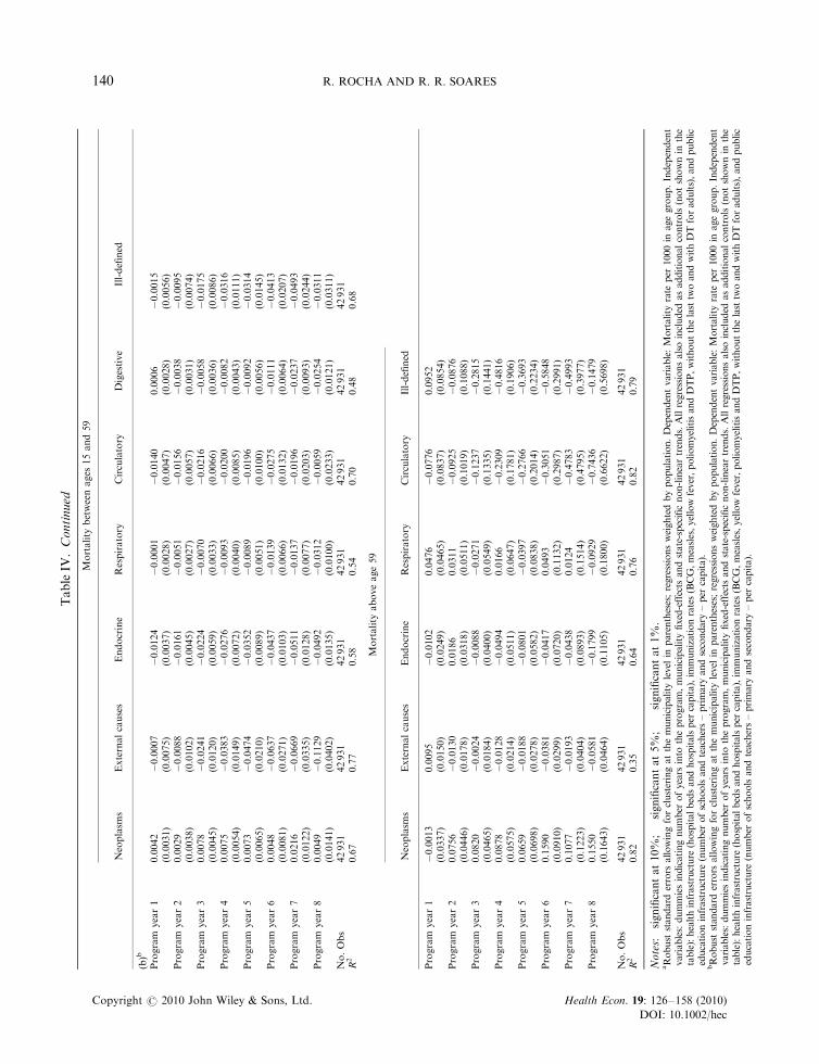
Table IV shows that, in the age group between 15 and 59, the Family Health Program appears as havingsignificant impacts on mortality due to external causes, endocrine, respiratory, circulatory, and digestivediseases. These are some of the causes of death that appeared as important in the age group between 1 and 4,plus circulatory and digestive diseases, which are typically adult conditions (including heart andcerebrovascular diseases, gastric ulcer, liver cirrhosis, and other liver diseases). Again, some of theseconditions can be affected – through changes in diet or behavior, for example – by the information,monitoring, and guidance provided by the Family Health Program. Quantitatively, the largest impacts onthis age group are observed for external causes, endocrine and respiratory diseases. For the populationabove 59, the evidence on the impacts of the program is rather weak. There are only some significant impactson mortality by ill-defined causes and, surprisingly, some positive impacts on mortality due to neoplasms.Since these are relatively small in magnitude and seem to appear precisely when there are significantreductions in mortality due to ill-defined conditions, we do not attach much weight to these results. It seemsfair to say that there is no consistent evidence on the effects of the program on mortality above 59.

5.3. Robustness of the impact on mortality

The main remaining concern in our specification is related to unobserved features of the dynamicbehavior of mortality, coupled with the possibility of endogeneity in the adoption of the program. Thismay be the case, for example, if the program dummies are just capturing pre-existing trends inmortality, rather than the impact of the intervention. It may also be the case if municipalities that startoff with high mortality tend to converge to lower mortality levels, as seems to be the case in recentdecades in Brazil (see Soares, 2007a). In this situation, if high mortality municipalities are also morelikely to adopt the program, one might attribute to the program an effect that is simply due to mortalityconvergence across municipalities.

Our analysis of the adoption of the program in Section 4.3 suggests that these concerns do not seemparticularly relevant. Table AII showed that adoption of the program was related to politicalconsiderations and initial characteristics of municipalities, but did not seem to be greatly affected byshocks to mortality. Still, we take these possibilities seriously and adopt two strategies to deal withthem. First, we introduce dummies indicating number of years before the program. If the effect of thePSF estimated before is due to pre-existing trends in mortality, these pre-program dummies should besignificant. Second, we introduce an interaction of a linear time trend with initial mortality. This allowseach municipality to converge to its state specific non-linear trend, at a rate that may vary with its initialconditions, so that municipalities with different mortality levels in 1993 may display different dynamics

15The Family Health Program is one of the ingredients of the National Policy of Urgency Attention (‘Polıtica Nacional deAtenc- ao as Urgencias’), being an integral part of a system of response to emergencies that includes a centralized system of rescuethrough the use of ambulances (‘Servic-o de Atendimento Movel de Urgencia’) and public and private hospitals.



DOI: 10.1002/hec

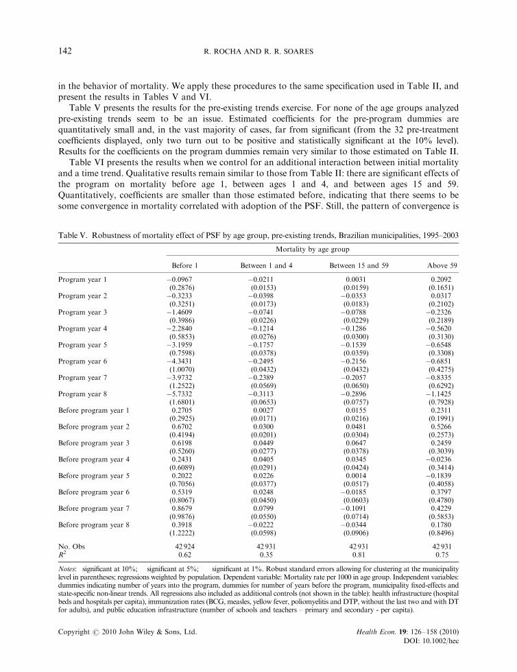
in the behavior of mortality. We apply these procedures to the same specification used in Table II, andpresent the results in Tables V and VI.

Table V presents the results for the pre-existing trends exercise. For none of the age groups analyzedpre-existing trends seem to be an issue. Estimated coefficients for the pre-program dummies arequantitatively small and, in the vast majority of cases, far from significant (from the 32 pre-treatmentcoefficients displayed, only two turn out to be positive and statistically significant at the 10% level).Results for the coefficients on the program dummies remain very similar to those estimated on Table II.

Table VI presents the results when we control for an additional interaction between initial mortalityand a time trend. Qualitative results remain similar to those from Table II: there are significant effects ofthe program on mortality before age 1, between ages 1 and 4, and between ages 15 and 59.Quantitatively, coefficients are smaller than those estimated before, indicating that there seems to besome convergence in mortality correlated with adoption of the PSF. Still, the pattern of convergence is

Table V. Robustness of mortality effect of PSF by age group, pre-existing trends, Brazilian municipalities, 1995–2003

Mortality by age group

Before 1 Between 1 and 4 Between 15 and 59 Above 59

Program year 1 �0.0967 �0.0211 0.0031 0.2092(0.2876) (0.0153) (0.0159) (0.1651)

Program year 2 �0.3233 �0.0398�� 0.0353� 0.0317(0.3251) (0.0173) (0.0183) (0.2102)

Program year 3 �1.4609�� 0.0741�� 0.0788�� 0.2326(0.3986) (0.0226) (0.0229) (0.2189)

Program year 4 �2.2840�� 0.1214�� 0.1286�� 0.5620�

(0.5853) (0.0276) (0.0300) (0.3130)Program year 5 �3.1959�� 0.1757�� 0.1539�� 0.6548��

(0.7598) (0.0378) (0.0359) (0.3308)Program year 6 �4.3431�� 0.2495�� 0.2156�� 0.6851

(1.0070) (0.0432) (0.0432) (0.4275)Program year 7 �3.9732�� 0.2389�� 0.2057�� 0.8335

(1.2522) (0.0569) (0.0650) (0.6292)Program year 8 �5.7332�� 0.3113�� 0.2896�� 1.1425

(1.6801) (0.0653) (0.0757) (0.7928)Before program year 1 0.2705 0.0027 0.0155 0.2311

(0.2925) (0.0171) (0.0216) (0.1991)Before program year 2 0.6702 0.0300 0.0481 0.5266��

(0.4194) (0.0201) (0.0304) (0.2573)Before program year 3 0.6198 0.0449 0.0647� 0.2459

(0.5260) (0.0277) (0.0378) (0.3039)Before program year 4 0.2431 0.0405 0.0345 �0.0236

(0.6089) (0.0291) (0.0424) (0.3414)Before program year 5 0.2022 0.0226 0.0014 �0.1839

(0.7056) (0.0377) (0.0517) (0.4058)Before program year 6 0.5319 0.0248 �0.0185 0.3797

(0.8067) (0.0450) (0.0603) (0.4780)Before program year 7 0.8679 0.0799 �0.1091 0.4229

(0.9876) (0.0550) (0.0714) (0.5853)Before program year 8 0.3918 �0.0222 �0.0344 0.1780

(1.2222) (0.0598) (0.0906) (0.8496)

No. Obs 42 924 42 931 42 931 42 931R2 0.62 0.35 0.81 0.75

Notes: �significant at 10%; ��significant at 5%; ��significant at 1%. Robust standard errors allowing for clustering at the municipalitylevel in parentheses; regressions weighted by population. Dependent variable: Mortality rate per 1000 in age group. Independent variables:dummies indicating number of years into the program, dummies for number of years before the program, municipality fixed-effects andstate-specific non-linear trends. All regressions also included as additional controls (not shown in the table): health infrastructure (hospitalbeds and hospitals per capita), immunization rates (BCG, measles, yellow fever, poliomyelitis and DTP, without the last two and with DTfor adults), and public education infrastructure (number of schools and teachers – primary and secondary - per capita).



DOI: 10.1002/hec

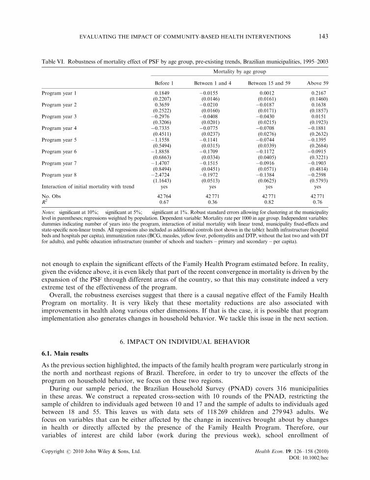
not enough to explain the significant effects of the Family Health Program estimated before. In reality,given the evidence above, it is even likely that part of the recent convergence in mortality is driven by theexpansion of the PSF through different areas of the country, so that this may constitute indeed a veryextreme test of the effectiveness of the program.

Overall, the robustness exercises suggest that there is a causal negative effect of the Family HealthProgram on mortality. It is very likely that these mortality reductions are also associated withimprovements in health along various other dimensions. If that is the case, it is possible that programimplementation also generates changes in household behavior. We tackle this issue in the next section.

6. IMPACT ON INDIVIDUAL BEHAVIOR

6.1. Main results

As the previous section highlighted, the impacts of the family health program were particularly strong inthe north and northeast regions of Brazil. Therefore, in order to try to uncover the effects of theprogram on household behavior, we focus on these two regions.

During our sample period, the Brazilian Household Survey (PNAD) covers 316 municipalitiesin these areas. We construct a repeated cross-section with 10 rounds of the PNAD, restricting thesample of children to individuals aged between 10 and 17 and the sample of adults to individuals agedbetween 18 and 55. This leaves us with data sets of 118 269 children and 279 943 adults. Wefocus on variables that can be either affected by the change in incentives brought about by changesin health or directly affected by the presence of the Family Health Program. Therefore, ourvariables of interest are child labor (work during the previous week), school enrollment of

Table VI. Robustness of mortality effect of PSF by age group, pre-existing trends, Brazilian municipalities, 1995–2003

Mortality by age group

Before 1 Between 1 and 4 Between 15 and 59 Above 59

Program year 1 0.1849 �0.0155 0.0012 0.2167(0.2207) (0.0146) (0.0161) (0.1460)

Program year 2 0.3659 �0.0210 �0.0187 0.1638(0.2522) (0.0160) (0.0171) (0.1857)

Program year 3 �0.2976 �0.0408�� 0.0430�� 0.0151(0.3206) (0.0201) (0.0215) (0.1923)

Program year 4 �0.7335 �0.0775�� 0.0708�� 0.1881(0.4511) (0.0237) (0.0276) (0.2632)

Program year 5 �1.1558�� 0.1141�� 0.0744�� 0.1395(0.5494) (0.0315) (0.0339) (0.2684)

Program year 6 �1.8858�� 0.1709�� 0.1172�� 0.0915(0.6863) (0.0334) (0.0405) (0.3221)

Program year 7 �1.4707� �0.1515�� 0.0916 �0.1903(0.8494) (0.0451) (0.0571) (0.4814)

Program year 8 �2.4724�� 0.1972�� 0.1384�� 0.2598(1.1643) (0.0513) (0.0625) (0.5793)

Interaction of initial mortality with trend yes yes yes yes

No. Obs 42 764 42 771 42 771 42 771R2 0.67 0.36 0.82 0.76

Notes: �significant at 10%; ��significant at 5%; ��significant at 1%. Robust standard errors allowing for clustering at the municipalitylevel in parentheses; regressions weighted by population. Dependent variable: Mortality rate per 1000 in age group. Independent variables:dummies indicating number of years into the program, interaction of initial mortality with linear trend, municipality fixed-effects andstate-specific non-linear trends. All regressions also included as additional controls (not shown in the table): health infrastructure (hospitalbeds and hospitals per capita), immunization rates (BCG, measles, yellow fever, poliomyelitis and DTP, without the last two and with DTfor adults), and public education infrastructure (number of schools and teachers – primary and secondary – per capita).



DOI: 10.1002/hec

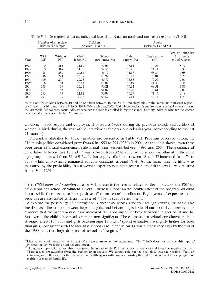
children,16 labor supply and employment of adults (work during the previous week), and fertility ofwomen (a birth during the year of the interview or the previous calendar year, corresponding to the last21 months).

Descriptive statistics for these variables are presented in Table VII. Program coverage among the316 municipalities considered grew from 0 in 1993 to 291 (92%) in 2004. As the table shows, even thesepoor areas of Brazil experienced substantial improvement between 1993 and 2004. The incidence ofchild labor between ages 10 and 17 was reduced from 32 to 20%, while school enrollment in the sameage group increased from 78 to 91%. Labor supply of adults between 18 and 55 increased from 74 to77%, while employment remained roughly constant, around 71%. At the same time, fertility – asmeasured by the probability that a woman experiences a birth over a 21 month interval – was reducedfrom 19 to 12%.

6.1.1. Child labor and schooling. Table VIII presents the results related to the impacts of the PSF onchild labor and school enrollment. Overall, there is almost no noticeable effect of the program on childlabor, while there seems to be a positive effect on school enrollment. Eight years of exposure to theprogram are associated with an increase of 4.5% in school enrollment.To explore the possibility of heterogeneous responses across genders and age groups, the table alsobreaks down the sample between boys and girls, and between ages 10 to 14 and 15 to 17. There is someevidence that the program may have increased the labor supply of boys between the ages of 10 and 14,but overall the child labor results remain non-significant. The estimates for school enrollment indicatestronger effects for boys and girls between ages 15 and 17 (point estimates are slightly higher for boysthan girls), consistent with the idea that school enrollment below 14 was already very high by the end ofthe 1990s and that boys drop out of school before girls.17

Table VII. Descriptive statistics, individual level data, Brazilian north and northeast regions, 1993–2004

Number of municipa-lities in the sample

Children(between 10 and 17)

Adults(between 18 and 55)

YearWithPSF

WithoutPSF

Childlabor (%)

Schoolenrollment (%)

Laborsupply (%)

Employment(%)

Fertility - birth last21 months

(% of women)

1993 0 316 31.69 77.65 73.64 70.55 18.791995 0 316 31.26 79.56 73.95 71.14 17.331996 28 288 25.65 81.17 71.87 68.86 16.681997 46 270 26.77 83.97 73.41 70.01 15.221998 109 207 27.33 86.77 73.93 70.35 15.061999 166 150 26.94 89.09 75.69 71.36 8.442001 243 73 22.51 90.21 74.34 69.51 13.872002 264 52 23.12 91.07 75.20 70.61 12.832003 273 43 21.92 90.99 76.29 71.14 12.182004 291 25 20.43 90.67 77.04 72.14 11.76

Note: Data for children between 10 and 17 or adults between 18 and 55; 316 municipalities in the north and northeast regions;calculated from 10 rounds of the PNAD (1993–2004, excluding 2000). Child labor and adult employment is defined as work duringthe last week. School enrollment indicates whether the child is enrolled in regular school. Fertility indicates whether the womanexperienced a birth over the last 21 months.

16Ideally, we would measure the impact of the program on school attendance. The PNAD does not provide this type ofinformation, so we focus on school enrollment.

17Though not reported here, we also investigated the impact of the PSF on teenage pregnancies and found no significant effects.These results are available from the authors upon request. We cannot rule out the possibility that the positive effects onschooling are spillovers from the interaction of health agents with families, possibly through counseling and advising regardingmultiple aspects of family life.



DOI: 10.1002/hec

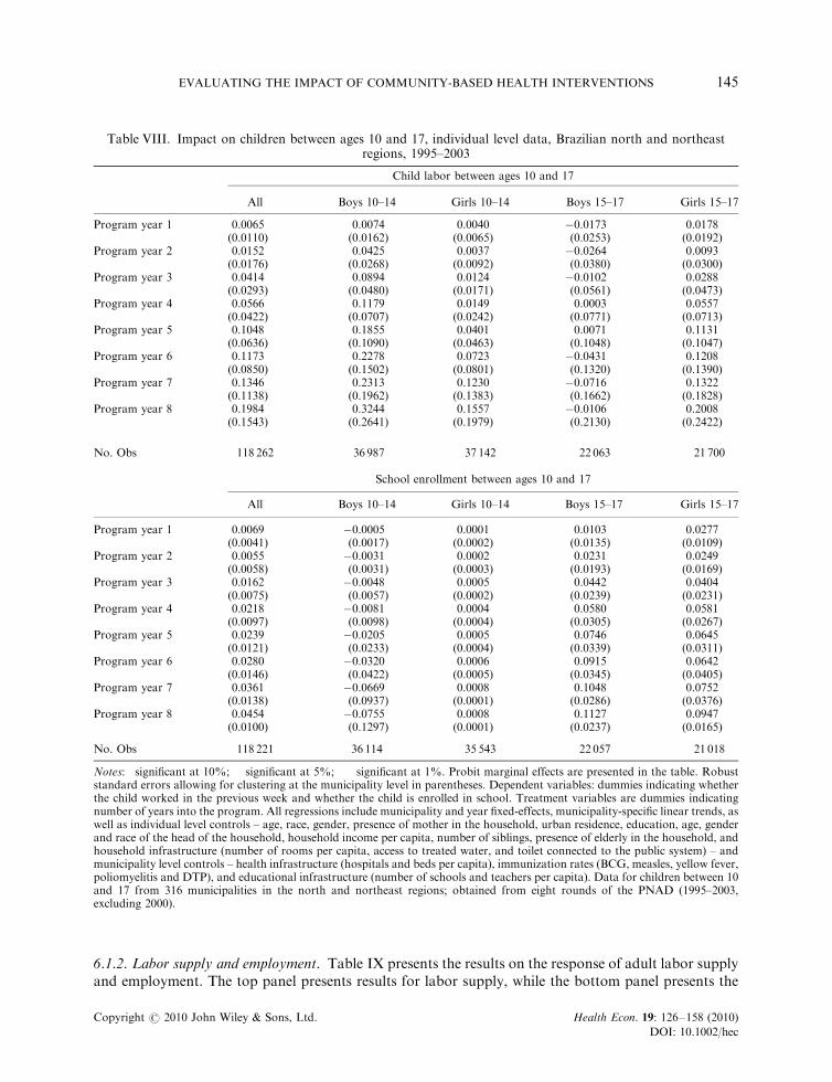
6.1.2. Labor supply and employment. Table IX presents the results on the response of adult labor supplyand employment. The top panel presents results for labor supply, while the bottom panel presents the

Table VIII. Impact on children between ages 10 and 17, individual level data, Brazilian north and northeastregions, 1995–2003

Child labor between ages 10 and 17

All Boys 10–14 Girls 10–14 Boys 15–17 Girls 15–17

Program year 1 0.0065 0.0074 0.0040 �0.0173 0.0178(0.0110) (0.0162) (0.0065) (0.0253) (0.0192)

Program year 2 0.0152 0.0425 0.0037 �0.0264 0.0093(0.0176) (0.0268) (0.0092) (0.0380) (0.0300)

Program year 3 0.0414 0.0894� 0.0124 �0.0102 0.0288(0.0293) (0.0480) (0.0171) (0.0561) (0.0473)

Program year 4 0.0566 0.1179� 0.0149 0.0003 0.0557(0.0422) (0.0707) (0.0242) (0.0771) (0.0713)

Program year 5 0.1048� 0.1855� 0.0401 0.0071 0.1131(0.0636) (0.1090) (0.0463) (0.1048) (0.1047)

Program year 6 0.1173 0.2278 0.0723 �0.0431 0.1208(0.0850) (0.1502) (0.0801) (0.1320) (0.1390)

Program year 7 0.1346 0.2313 0.1230 �0.0716 0.1322(0.1138) (0.1962) (0.1383) (0.1662) (0.1828)

Program year 8 0.1984 0.3244 0.1557 �0.0106 0.2008(0.1543) (0.2641) (0.1979) (0.2130) (0.2422)

No. Obs 118 262 36 987 37 142 22 063 21 700

School enrollment between ages 10 and 17

All Boys 10–14 Girls 10–14 Boys 15–17 Girls 15–17

Program year 1 0.0069� �0.0005 0.0001 0.0103 0.0277��

(0.0041) (0.0017) (0.0002) (0.0135) (0.0109)Program year 2 0.0055 �0.0031 0.0002 0.0231 0.0249

(0.0058) (0.0031) (0.0003) (0.0193) (0.0169)Program year 3 0.0162�� 0.0048 0.0005�� 0.0442� 0.0404�

(0.0075) (0.0057) (0.0002) (0.0239) (0.0231)Program year 4 0.0218�� 0.0081 0.0004 0.0580� 0.0581��

(0.0097) (0.0098) (0.0004) (0.0305) (0.0267)Program year 5 0.0239�� 0.0205 0.0005 0.0746�� 0.0645��

(0.0121) (0.0233) (0.0004) (0.0339) (0.0311)Program year 6 0.0280� �0.0320 0.0006 0.0915�� 0.0642

(0.0146) (0.0422) (0.0005) (0.0345) (0.0405)Program year 7 0.0361�� 0.0669 0.0008�� 0.1048�� 0.0752��

(0.0138) (0.0937) (0.0001) (0.0286) (0.0376)Program year 8 0.0454�� 0.0755 0.0008�� 0.1127�� 0.0947��

(0.0100) (0.1297) (0.0001) (0.0237) (0.0165)

No. Obs 118 221 36 114 35 543 22 057 21 018

Notes: �significant at 10%; ��significant at 5%; ��significant at 1%. Probit marginal effects are presented in the table. Robuststandard errors allowing for clustering at the municipality level in parentheses. Dependent variables: dummies indicating whetherthe child worked in the previous week and whether the child is enrolled in school. Treatment variables are dummies indicatingnumber of years into the program. All regressions include municipality and year fixed-effects, municipality-specific linear trends, aswell as individual level controls – age, race, gender, presence of mother in the household, urban residence, education, age, genderand race of the head of the household, household income per capita, number of siblings, presence of elderly in the household, andhousehold infrastructure (number of rooms per capita, access to treated water, and toilet connected to the public system) – andmunicipality level controls – health infrastructure (hospitals and beds per capita), immunization rates (BCG, measles, yellow fever,poliomyelitis and DTP), and educational infrastructure (number of schools and teachers per capita). Data for children between 10and 17 from 316 municipalities in the north and northeast regions; obtained from eight rounds of the PNAD (1995–2003,excluding 2000).



DOI: 10.1002/hec

results for employment. Results are shown for both genders (ages between 18 and 55), and for men andwomen separately.18

The table suggests a consistent effect of the PSF on adult labor supply and employment.Municipalities 8 years into the program have adult labor supply 6.8 percentage points higher andemployment 11 percentage points higher than otherwise equivalent municipalities not covered by theprogram. Quantitative results for both labor supply and employment are stronger for women than formen; though significance is reduced as the sample is broken down by gender. Point estimate seems to besomewhat too large quantitatively, but the overall pattern does seem to suggest a positive correlationbetween program implementation and adult employment.

6.1.3. Fertility. Table X presents the results related to fertility (probability of a birth over the 21 monthspreceding the interview). Implementation of the PSF seems to be systematically associated with reducedprobability of women experiencing births. The average effect for women between ages 18 and55 registered in the first column is due mostly to women between 31 and 40, though there are alsonegative but mostly non-significant impacts for women between 18 and 30. Given that Table X showedevidence of positive impacts of the program on labor supply and employment of women, the impact onfertility may be either due to better access to – or information about – contraceptive techniques, or dueto improved health of adults and existing children (change in long-term lifetime decision on laborsupply affecting fertility choice). Also, the age profile of the estimated response is consistent with whatshould be expected: we find no significant effect of the PSF on fertility between 41 and 55, an age groupwhere fertility is typically much lower and undesired pregnancies much rarer.

Quantitatively, the estimated coefficients for the age group between 31 and 40 imply that, formunicipalities 5 years into the program, women are 4.6 percentage points less likely to haveexperienced a birth in the previous 21 months than otherwise identical women in municipalities notcovered by the PSF. The analogous number for municipalities 8 years into the program is 6.5 percentagepoints.

Overall, the evidence suggests that the Family Health Program reduced fertility, increased femalelabor supply, and improved school enrollment of children. These effects are consistent with what shouldbe expected from improvements in access to health and their effects on decisions related to humancapital, number of children, and labor supply.

6.2. Heterogeneity in response

In order to better understand the impact of the Family Health Program on household decisions, weexplore some dimensions of potential heterogeneity in response. In this section, we look at thesignificant results from the previous tables and investigate heterogeneity in response in relation to thelocation where the family lives (rural vs. urban) and to conditions of the household (no access to treatedwater and no access to the public sewage system). Table XI presents a synthesis of the main results.

The table shows that the effect on school enrollment is stronger for households in rural areas and for thosewithout access to treated water. The coefficients for municipalities 8 years into the program for these tworegressions are, respectively, 0.058 and 0.064, as compared to 0.045 in the main specification presented before.

For adult labor supply and employment, effects are also much stronger in rural areas. The resultsappear as significant and of magnitude similar to that observed on Table IX for households withouttoilet connected to the public sewage system. In the cases of both child schooling and adult labor, theimpact of the program seems to be associated with poor households in rural areas, possibly with lessaccess to the public health system.

18We also tried regressions disaggregated by age group in this case, but results were rarely significant and did not shed much light.



DOI: 10.1002/hec

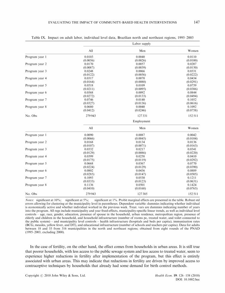
In the case of fertility, on the other hand, the effect comes from households in urban areas. It is still truethat poorer households, with less access to the public sewage system and less access to treated water, seem toexperience higher reductions in fertility after implementation of the program, but this effect is entirelyassociated with urban areas. This may indicate that reductions in fertility are driven by improved access tocontraceptive techniques by households that already had some demand for birth control methods.

Table IX. Impact on adult labor, individual level data, Brazilian north and northeast regions, 1995–2003

Labor supply

All Men Women

Program year 1 0.0103� 0.0040 0.0110(0.0056) (0.0026) (0.0100)

Program year 2 0.0170� 0.0057 0.0207(0.0087) (0.0039) (0.0150)

Program year 3 0.0248�� 0.0066 0.0331(0.0122) (0.0056) (0.0222)

Program year 4 0.0317� 0.0070 0.0434(0.0164) (0.0080) (0.0291)

Program year 5 0.0518�� 0.0109 0.0759��

(0.0211) (0.0095) (0.0386)Program year 6 0.0568�� 0.0092 0.0844�

(0.0272) (0.0133) (0.0494)Program year 7 0.0746�� 0.0140 0.1052�

(0.0327) (0.0136) (0.0616)Program year 8 0.0680� 0.0040 0.1092

(0.0412) (0.0246) (0.0758)

No. Obs 279 943 127 331 152 511

Employment

All Men Women

Program year 1 0.0090 0.0087� 0.0042(0.0066) (0.0045) (0.0104)

Program year 2 0.0168 0.0134� 0.0136(0.0107) (0.0071) (0.0163)

Program year 3 0.0332�� 0.0217�� 0.0341(0.0129) (0.0086) (0.0220)

Program year 4 0.0399�� 0.0258�� 0.0410(0.0175) (0.0119) (0.0292)

Program year 5 0.0668�� 0.0367�� 0.0770��

(0.0224) (0.0129) (0.0390)Program year 6 0.0802�� 0.0436�� 0.0889�

(0.0285) (0.0147) (0.0505)Program year 7 0.1093�� 0.0530�� 0.1211�

(0.0333) (0.0123) (0.0631)Program year 8 0.1136�� 0.0501�� 0.1424�

(0.0410) (0.0168) (0.0765)

No. Obs 279 943 127 385 152 511

Notes: �significant at 10%; ��significant at 5%; ��significant at 1%. Probit marginal effects are presented in the table. Robust stderrors allowing for clustering at the municipality level in parentheses. Dependent variable: dummies indicating whether individualis economically active and whether individual worked in the previous week. Treat. vars are dummies indicating number of yearsinto the program. All regs include municipality and year fixed-effects, municipality-specific linear trends, as well as individual levelcontrols – age, race, gender, education, presence of spouse in the household, urban residence, metropolitan region, presence ofelderly and children in the household, and household infrastructure (number of rooms pc, treated water, and toilet connected tothe public system) – and municipality level controls – health infrastructure (hospitals and beds per capita), immunization rates(BCG, measles, yellow fever, and DT), and educational infrastructure (number of schools and teachers per capita). Data for adultsbetween 18 and 55 from 316 municipalities in the north and northeast regions; obtained from eight rounds of the PNAD(1995–2003, excluding 2000).



DOI: 10.1002/hec

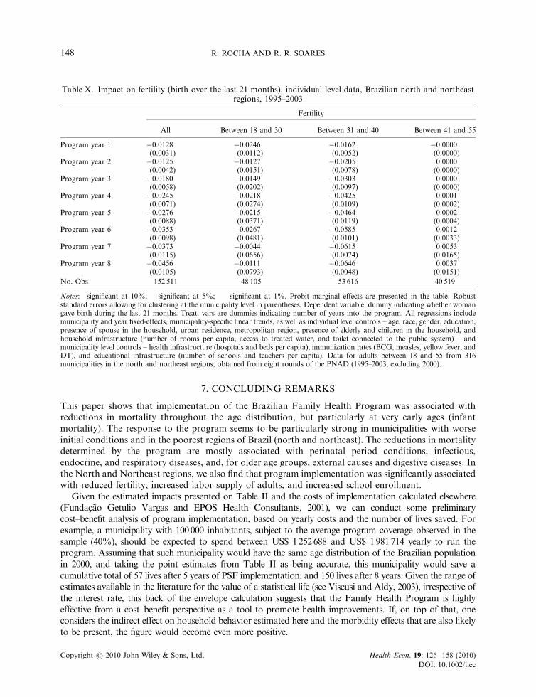
7. CONCLUDING REMARKS

This paper shows that implementation of the Brazilian Family Health Program was associated withreductions in mortality throughout the age distribution, but particularly at very early ages (infantmortality). The response to the program seems to be particularly strong in municipalities with worseinitial conditions and in the poorest regions of Brazil (north and northeast). The reductions in mortalitydetermined by the program are mostly associated with perinatal period conditions, infectious,endocrine, and respiratory diseases, and, for older age groups, external causes and digestive diseases. Inthe North and Northeast regions, we also find that program implementation was significantly associatedwith reduced fertility, increased labor supply of adults, and increased school enrollment.

Given the estimated impacts presented on Table II and the costs of implementation calculated elsewhere(Fundac-ao Getulio Vargas and EPOS Health Consultants, 2001), we can conduct some preliminarycost–benefit analysis of program implementation, based on yearly costs and the number of lives saved. Forexample, a municipality with 100000 inhabitants, subject to the average program coverage observed in thesample (40%), should be expected to spend between US$ 1252688 and US$ 1981714 yearly to run theprogram. Assuming that such municipality would have the same age distribution of the Brazilian populationin 2000, and taking the point estimates from Table II as being accurate, this municipality would save acumulative total of 57 lives after 5 years of PSF implementation, and 150 lives after 8 years. Given the range ofestimates available in the literature for the value of a statistical life (see Viscusi and Aldy, 2003), irrespective ofthe interest rate, this back of the envelope calculation suggests that the Family Health Program is highlyeffective from a cost–benefit perspective as a tool to promote health improvements. If, on top of that, oneconsiders the indirect effect on household behavior estimated here and the morbidity effects that are also likelyto be present, the figure would become even more positive.

Table X. Impact on fertility (birth over the last 21 months), individual level data, Brazilian north and northeastregions, 1995–2003

Fertility

All Between 18 and 30 Between 31 and 40 Between 41 and 55

Program year 1 �0.0128�� 0.0246�� 0.0162�� 0.0000(0.0031) (0.0112) (0.0052) (0.0000)

Program year 2 �0.0125�� 0.0127 �0.0205�� 0.0000(0.0042) (0.0151) (0.0078) (0.0000)

Program year 3 �0.0180�� 0.0149 �0.0303�� 0.0000(0.0058) (0.0202) (0.0097) (0.0000)

Program year 4 �0.0245�� 0.0218 �0.0425�� 0.0001(0.0071) (0.0274) (0.0109) (0.0002)

Program year 5 �0.0276�� 0.0215 �0.0464�� 0.0002(0.0088) (0.0371) (0.0119) (0.0004)

Program year 6 �0.0353�� 0.0267 �0.0585�� 0.0012(0.0098) (0.0481) (0.0101) (0.0033)

Program year 7 �0.0373�� 0.0044 �0.0615�� 0.0053(0.0115) (0.0656) (0.0074) (0.0165)

Program year 8 �0.0456�� 0.0111 �0.0646�� 0.0037(0.0105) (0.0793) (0.0048) (0.0151)

No. Obs 152 511 48 105 53 616 40 519

Notes: �significant at 10%; ��significant at 5%; ��significant at 1%. Probit marginal effects are presented in the table. Robuststandard errors allowing for clustering at the municipality level in parentheses. Dependent variable: dummy indicating whether womangave birth during the last 21 months. Treat. vars are dummies indicating number of years into the program. All regressions includemunicipality and year fixed-effects, municipality-specific linear trends, as well as individual level controls – age, race, gender, education,presence of spouse in the household, urban residence, metropolitan region, presence of elderly and children in the household, andhousehold infrastructure (number of rooms per capita, access to treated water, and toilet connected to the public system) – andmunicipality level controls – health infrastructure (hospitals and beds per capita), immunization rates (BCG, measles, yellow fever, andDT), and educational infrastructure (number of schools and teachers per capita). Data for adults between 18 and 55 from 316municipalities in the north and northeast regions; obtained from eight rounds of the PNAD (1995–2003, excluding 2000).



DOI: 10.1002/hec

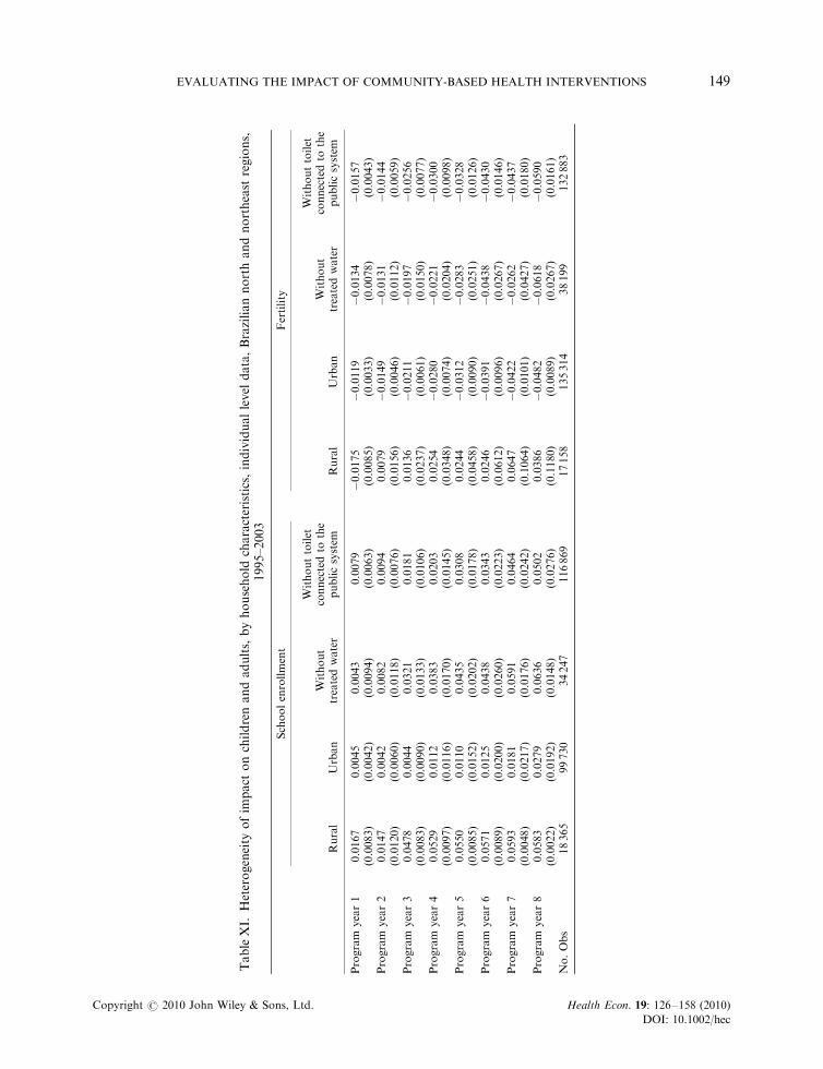
TableXI.

Heterogeneity

ofim

pact

onchildrenandadults,byhousehold

characteristics,individuallevel

data,Braziliannorthandnortheast

regions,

1995–2003

Schoolenrollment

Fertility

Rural

Urban

Without

treatedwater

Withouttoilet

connectedto

the

publicsystem

Rural

Urban

Without

treatedwater

Withouttoilet

connectedto

the

publicsystem

Program

year1

0.0167��

0.0045

0.0043

0.0079

�0.0175��

�0.0119��

�0.0134�

�0.0157��

(0.0083)

(0.0042)

(0.0094)

(0.0063)

(0.0085)

(0.0033)

(0.0078)

(0.0043)

Program

year2

0.0147

0.0042

0.0082

0.0094

0.0079

�0.0149��

�0.0131

�0.0144��

(0.0120)

(0.0060)

(0.0118)

(0.0076)

(0.0156)

(0.0046)

(0.0112)

(0.0059)

Program

year3

0.0478��

0.0044

0.0321��

0.0181�

0.0136

�0.0211��

�0.0197

�0.0256��

(0.0083)

(0.0090)

(0.0133)

(0.0106)

(0.0237)

(0.0061)

(0.0150)

(0.0077)

Program

year4

0.0529��

0.0112

0.0383��

0.0203

0.0254

�0.0280��

�0.0221

�0.0300��

(0.0097)

(0.0116)

(0.0170)

(0.0145)

(0.0348)

(0.0074)

(0.0204)

(0.0098)

Program

year5

0.0550��

0.0110

0.0435��

0.0308�

0.0244

�0.0312��

�0.0283

�0.0328��

(0.0085)

(0.0152)

(0.0202)

(0.0178)

(0.0458)

(0.0090)

(0.0251)

(0.0126)

Program

year6

0.0571��

0.0125

0.0438�

0.0343

0.0246

�0.0391��

�0.0438

�0.0430��

(0.0089)

(0.0200)

(0.0260)

(0.0223)

(0.0612)

(0.0096)

(0.0267)

(0.0146)

Program

year7

0.0593��

0.0181

0.0591��

0.0464�

0.0647

�0.0422��

�0.0262

�0.0437��

(0.0048)

(0.0217)

(0.0176)

(0.0242)

(0.1064)

(0.0101)

(0.0427)

(0.0180)

Program

year8

0.0583��

0.0279

0.0636��

0.0502�

0.0386

�0.0482��

�0.0618��

�0.0590��

(0.0022)

(0.0192)

(0.0148)

(0.0276)

(0.1180)

(0.0089)

(0.0267)

(0.0161)

No.Obs

18365

99730

34247

116869

17158

135314

38199

132883



DOI: 10.1002/hec

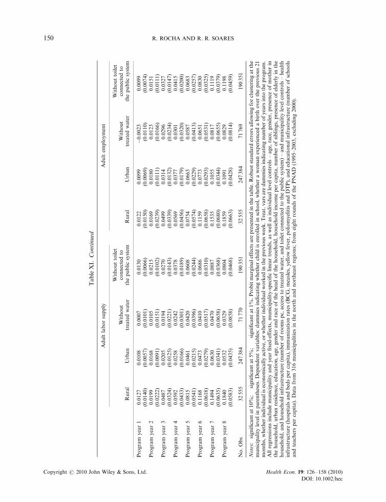
Adultlaborsupply

Adultem

ployment

Rural

Urban

Without

treatedwater

Withouttoilet

connectedto

thepublicsystem

Rural

Urban

Without

treatedwater

Withouttoilet

connectedto

thepublicsystem

Program

year1

0.0127

0.0108�

0.0007

0.0130��

0.0122

0.0099

�0.0023

0.0099

(0.0140)

(0.0057)

(0.0101)

(0.0066)

(0.0150)

(0.0069)

(0.0110)

(0.0074)

Program

year2

0.0199

0.0168�

0.0105

0.0215��

0.0169

0.0180

0.0123

0.0151

(0.0222)

(0.0091)

(0.0151)

(0.0102)

(0.0239)

(0.0111)

(0.0166)

(0.0111)

Program

year3

0.0487

0.0205�

0.0194

0.0270�

0.0499

0.0314��

0.0296

0.0327��

(0.0324)

(0.0125)

(0.0221)

(0.0143)

(0.0339)

(0.0132)

(0.0234)

(0.0147)

Program

year4

0.0592

0.0258

0.0242

0.0378��

0.0569

0.0377��

0.0301

0.0415��

(0.0433)

(0.0166)

(0.0301)

(0.0189)

(0.0456)

(0.0179)

(0.0320)

(0.0200)

Program

year5

0.0815

0.0461��

0.0420

0.0608��

0.0754

0.0663��

0.0587

0.0683��

(0.0541)

(0.0215)

(0.0396)

(0.0244)

(0.0574)

(0.0229)

(0.0413)

(0.0257)

Program

year6

0.1168�

0.0473�

0.0410

0.0686��

0.1159�

0.0773��

0.0651

0.0830��

(0.0618)

(0.0279)

(0.0517)

(0.0310)

(0.0658)

(0.0293)

(0.0531)

(0.0325)

Program

year7

0.1494��

0.0630�

0.0470

0.0887��

0.1535��

0.1055��

0.0817

0.1119��

(0.0635)

(0.0341)

(0.0658)

(0.0368)

(0.0680)

(0.0344)

(0.0655)

(0.0379)

Program

year8

0.1840��

0.0532

0.0329

0.0804�

0.1859��

0.1091��

0.0829

0.1198��

(0.0583)

(0.0435)

(0.0858)

(0.0468)

(0.0663)

(0.0428)

(0.0814)

(0.0459)

No.Obs

32555

247384

71770

190351

32555

247384

71769

190351

Notes:� significantat10%;��

significantat5%


.Probitmarginaleffectsare

presentedin

thetable.Robuststandard

errors

allowingforclusteringatthe

municipality

level

inparentheses.Dependentvariables:dummiesindicatingwhether

childisenrolled

inschool,whether

awomanexperiencedabirth

over

theprevious21

months,whether

individualiseconomicallyactive,orwhether

individualworked

inthepreviousweek.Treat.vars

are

dummiesindicatingnumber

ofyears

into

theprogram.

Allregressionsincludemunicipality

andyearfixed-effects,municipality-specificlineartrends,aswellasindividuallevel

controls–age,

race,gender,presence

ofmother

inthehousehold,urbanresidence,education,age,

gender

andrace

oftheheadofthehousehold,household

incomeper

capita,number

ofsiblings,presence

ofelderly

inthe

household,andhousehold

infrastructure

(number

ofroomspc,accessto

treatedwater,andtoilet

connectedto

thepublicsystem

)–andmunicipality

levelcontrols–health

infrastructure

(hospitalsandbedsper

capita),im


fever,poliomyelitisandDTP),andeducationalinfrastructure

(number

ofschools

andteachersper

capita).Data

from

316municipalities

inthenorthandnortheast

regions;from

eightroundsofthePNAD

(1995–2003,excluding2000).

TableXI.

Continued



DOI: 10.1002/hec

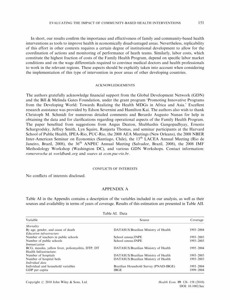
In short, our results confirm the importance and effectiveness of family and community-based healthinterventions as tools to improve health in economically disadvantaged areas. Nevertheless, replicabilityof this effort in other contexts requires a certain degree of institutional development to allow for thecoordination of actions and monitoring of performance of heath teams. Similarly, labor costs, whichconstitute the highest fraction of costs of the Family Health Program, depend on specific labor marketconditions and on the wage differentials required to convince medical doctors and health professionalsto work in the relevant regions. These aspects should be explicitly taken into account when consideringthe implementation of this type of intervention in poor areas of other developing countries.

ACKNOWLEDGEMENTS

The authors gratefully acknowledge financial support from the Global Development Network (GDN)and the Bill & Melinda Gates Foundation, under the grant program ‘Promoting Innovative Programsfrom the Developing World: Towards Realizing the Health MDGs in Africa and Asia.’ Excellentresearch assistance was provided by Edson Severnini and Hamilton Kai. The authors also wish to thankChristoph M. Schmidt for numerous detailed comments and Berardo Augusto Nunan for help inobtaining the data and for clarifications regarding operational aspects of the Family Health Program.The paper benefited from suggestions from Angus Deaton, Shubhashis Gangopadhyay, ErnestoSchargrodsky, Jeffrey Smith, Lyn Squire, Ranjeeta Thomas, and seminar participants at the HarvardSchool of Public Health, IPEA-Rio, PUC-Rio, the 2008 AEA Meetings (New Orleans), the 2008 NBERInter-American Seminar on Economics (Santiago, Chile), the 13th LACEA Annual Meeting (Rio deJaneiro, Brazil, 2008), the 36th ANPEC Annual Meeting (Salvador, Brazil, 2008), the 2008 IMFMethodology Workshop (Washington DC), and various GDN Workshops. Contact information:romerorocha at worldbank.org and soares at econ.puc-rio.br.

CONFLICTS OF INTERESTS

No conflicts of interests disclosed.

APPENDIX A

Table AI in the Appendix contains a description of the variables included in our analysis, as well as theirsources and availability in terms of years of coverage. Results of this estimation are presented in Table AII.

Table AI. Data

Variable Source Coverage

MortalityBy age, gender, and cause of death DATASUS/Brazilian Ministry of Health 1993–2004Education infrastructureNumber of teachers in public schools School census/INPE 1993–2003Number of public schools School census/INPE 1993–2003ImmunizationBCG, measles, yellow fever, poliomyelitis, DTP, DT DATASUS/Brazilian Ministry of Health 1995–2004Health Infrastructure:Number of hospitals DATASUS/Brazilian Ministry of Health 1993–2003Number of hospital beds DATASUS/Brazilian Ministry of Health 1993–2003Individual dataIndividual and household variables Brazilian Household Survey (PNAD-IBGE) 1993–2004GDP per capita IBGE 1999–2004



DOI: 10.1002/hec

TableAII.Hazard

estimationoftheprobabilityofjoiningthePSF,BrazilianMunicipalities,1993–2004

Probabilityofjoiningtheprogram

Dt�

1mortality

before1

�0.0004

�0.0005

(0.0009)

(0.0009)

Dt�

2mortality

before1

0.0020��

0.0020��

(0.0009)

(0.0009)

Dt�

3mortality

before1

0.0021��

0.0022��

(0.0009)

(0.0009)

Dt�

1mortality

between1and4

0.0004

(0.0094)

Dt�

2mortality

between1and4

�0.0131

(0.0095)

Dt�

3mortality

between1and4

0.0201��

(0.0095)

Dt�

1mortality

between15and59

0.0261��

(0.0133)

Dt�

2mortality

between15and59

�0.0070

(0.0131)

Dt�

3mortality

between15and59

�0.0282��

(0.0131)

Tim

e-varyingdim

ensionsofpublicpolicy

Dt�

1hospitalsper

1000

�0.0248��

�0.0252��

�0.0242��

�0.0250��

�0.0252��

�0.0244��

(0.0072)

(0.0076)

(0.0074)

(0.0075)

(0.0076)

(0.0075)

Dt�

1schoolsper

capita

�113.4947��

�113.3292��

�113.5942��

�113.7860��

�113.4989��

�113.7806��

(7.3298)

(7.4218)

(7.4668)

(8.1608)

(7.4315)

(7.4250)

Dt�

1hospitalbedsper

1000

�0.0047

�0.0043

�0.0053

�0.0054

�0.0045

�0.0057

(0.0180)

(0.0189)

(0.0185)

(0.0187)

(0.0189)

(0.0188)

Dt�

1teachersper

capita

14.6307��

14.5597��

14.6325��

14.6092��

14.6272��

14.6974��

(2.6987)

(2.7246)

(2.7016)

(2.7192)

(2.7312)

(2.7228)

PartyoftheMayor

WorkersParty(PT)

0.3090��

0.3097��

0.3094��

0.3110��

0.3119��

0.3105��

(0.0973)

(0.0971)

(0.0970)

(0.0972)

(0.0972)

(0.0972)

SocialDem

ocratParty(PSDB)

0.1684��

0.1690��

0.1670��

0.1672��

0.1672��

0.1665��

(0.0464)

(0.0465)

(0.0466)

(0.0463)

(0.0465)

(0.0464)

BrazilianLaborParty(PTB)

�0.1262��

�0.1259��

�0.1263��

�0.1265��

�0.1256��

�0.1252��

(0.0628)

(0.0628)

(0.0627)

(0.0631)

(0.0629)

(0.0628)

ProgressistParty(PP)

0.0260

0.0263

0.0267

0.0272

0.0280

0.0273

(0.0544)

(0.0534)

(0.0534)

(0.0535)

(0.0534)

(0.0534)

LiberalFrontParty(PFL)

0.0106

0.0107

0.0108

0.0125

0.0125

0.0134

(0.0458)

(0.0457)

(0.0454)

(0.0483)

(0.0458)

(0.0458)

Dem

ocraticLaborParty(PDT)

�0.0805

�0.0798

�0.0809

�0.0818

�0.0797

�0.0803

(0.0661)

(0.0661)

(0.0661)

(0.0664)

(0.0661)

(0.0661)



DOI: 10.1002/hec

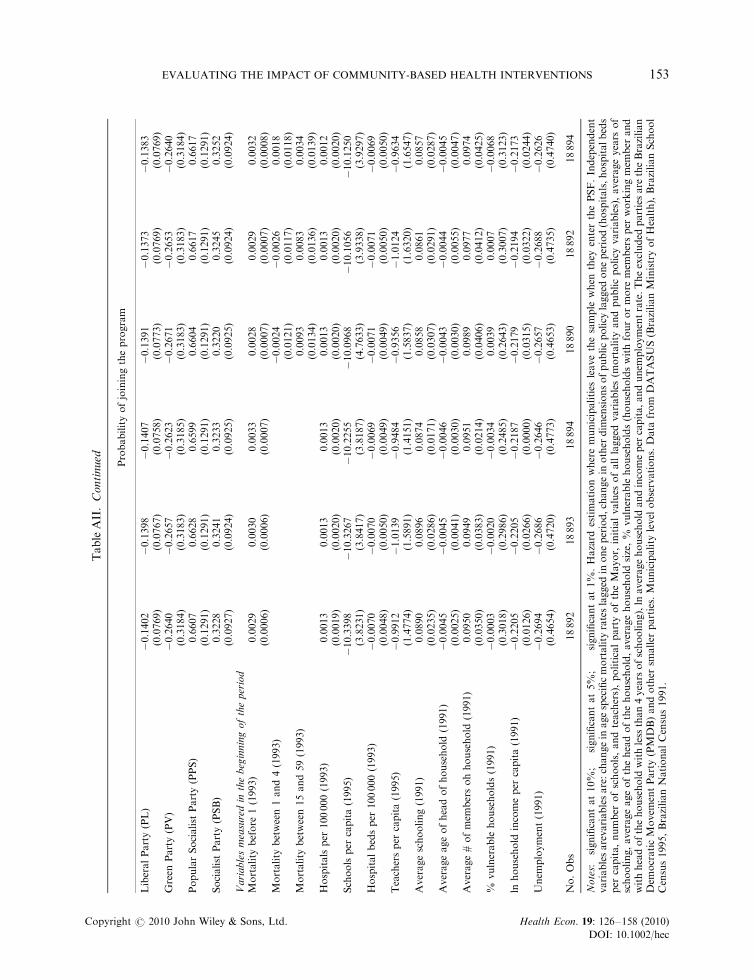
TableAII.Continued Probabilityofjoiningtheprogram

LiberalParty(PL)

�0.1402�

�0.1398�

�0.1407�

�0.1391�

�0.1373�

�0.1383�

(0.0769)

(0.0767)

(0.0758)

(0.0773)

(0.0769)

(0.0769)

Green

Party(PV)

�0.2640

�0.2657

�0.2623

�0.2671

�0.2653

�0.2640

(0.3184)

(0.3183)

(0.3185)

(0.3183)

(0.3183)

(0.3184)

PopularSocialist

Party(PPS)

0.6607��

0.6628��

0.6599��

0.6604��

0.6617��

0.6617��

(0.1291)

(0.1291)

(0.1291)

(0.1291)

(0.1291)

(0.1291)

Socialist

Party(PSB)

0.3228��

0.3241��

0.3233��

0.3220��

0.3245��

0.3252��

(0.0927)

(0.0924)

(0.0925)

(0.0925)

(0.0924)

(0.0924)

Variablesmeasuredin

thebeginningoftheperiod

Mortality

before

1(1993)

0.0029��

0.0030��

0.0033��

0.0028��

0.0029��

0.0032��

(0.0006)

(0.0006)

(0.0007)

(0.0007)

(0.0007)

(0.0008)

Mortality

between1and4(1993)

�0.0024

�0.0026

0.0018

(0.0121)

(0.0117)

(0.0118)

Mortality

between15and59(1993)

0.0093

0.0083

0.0034

(0.0134)

(0.0136)

(0.0139)

Hospitalsper

100000(1993)

0.0013

0.0013

0.0013

0.0013

0.0013

0.0012

(0.0019)

(0.0020)

(0.0020)

(0.0020)

(0.0020)

(0.0020)

Schoolsper

capita(1995)

�10.3398��

�10.3267��

�10.2255��

�10.0968��

�10.1056��

�10.1250��

(3.8231)

(3.8417)

(3.8187)

(4.7633)

(3.9338)

(3.9297)

Hospitalbedsper

100000(1993)

�0.0070

�0.0070

�0.0069

�0.0071

�0.0071

�0.0069

(0.0048)

(0.0050)

(0.0049)

(0.0049)

(0.0050)

(0.0050)

Teachersper

capita(1995)

�0.9912

�1.0139

�0.9484

�0.9356

�1.0124

�0.9634

(1.4774)

(1.5891)

(1.4151)

(1.5837)

(1.6320)

(1.6547)

Averageschooling(1991)

0.0890��

0.0896��

0.0874��

0.0858��

0.0861��

0.0857��

(0.0235)

(0.0286)

(0.0171)

(0.0307)

(0.0291)

(0.0287)

Averageageofheadofhousehold

(1991)

�0.0045�

�0.0045

�0.0046

�0.0043

�0.0044

�0.0045

(0.0025)

(0.0041)

(0.0030)

(0.0030)

(0.0055)

(0.0047)

Average#ofmem

bersohhousehold

(1991)

0.0950��

0.0949��

0.0951��

0.0989��

0.0977��

0.0974��

(0.0350)

(0.0383)

(0.0214)

(0.0406)

(0.0412)

(0.0425)

%vulnerable

households(1991)

�0.0003

�0.0020

�0.0034

0.0039

0.0007

�0.0068

(0.3018)

(0.2986)

(0.2485)

(0.2643)

(0.3007)

(0.3123)

lnhousehold

incomeper

capita(1991)

�0.2205��

�0.2205��

�0.2187

�0.2179��

�0.2194��

�0.2173��

(0.0126)

(0.0266)

(0.0000)

(0.0315)

(0.0322)

(0.0244)

Unem

ployment(1991)

�0.2694

�0.2686

�0.2646

�0.2657

�0.2688

�0.2626

(0.4654)

(0.4720)

(0.4773)

(0.4653)

(0.4735)

(0.4740)

No.Obs

18892

18893

18894

18890

18892

18894


;��

significantat5%


.Hazard

estimationwheremunicipalities

leavethesample

when

they

enterthePSF.Independent

variablesarevariablesare:changein

agespecificmortality

rateslagged

inoneperiod,changein

other

dim

ensionsofpublicpolicy

lagged

oneperiod(hospitals,hospitalbeds

per

capita,number

ofschools,andteachers),politicalpartyoftheMayor,

initialvalues

ofalllagged

variables(m

ortality

andpublicpolicy

variables),averageyears

of

schooling,averageageoftheheadofthehousehold,averagehousehold

size,%

vulnerable

households(householdswithfourormore

mem

bersper

workingmem

ber

and

withheadofthehousehold

withless

than4years

ofschooling),ln

averagehousehold

andincomeper

capita,andunem

ploymentrate.Theexcluded

partiesare

theBrazilian

Dem

ocraticMovem

entParty(PMDB)andother

smaller

parties.Municipality

level

observations.Data

from

DATASUS(BrazilianMinistryofHealth),BrazilianSchool

Census1995,BrazilianNationalCensus1991.



DOI: 10.1002/hec

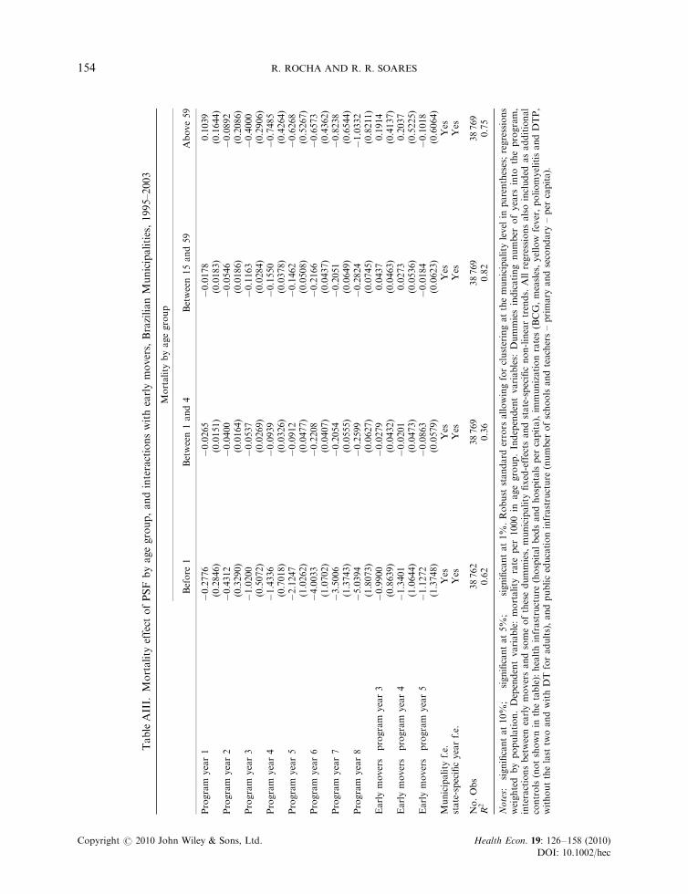
TableAIII.

Mortality

effect

ofPSF

byagegroup,andinteractionswithearlymovers,BrazilianMunicipalities,1995–2003

Mortality

byagegroup

Before

1Between1and4

Between15and59

Above59

Program

year1

�0.2776

�0.0265�

�0.0178

0.1039

(0.2846)

(0.0151)

(0.0183)

(0.1644)

Program

year2

�0.4312

�0.0400��

�0.0546��

�0.0892

(0.3290)

(0.0164)

(0.0186)

(0.2086)

Program

year3

�1.0200��

�0.0537��

�0.1163��

�0.4000

(0.5072)

(0.0269)

(0.0284)

(0.2906)

Program

year4

�1.4336��

�0.0939��

�0.1550��

�0.7485�

(0.7018)

(0.0326)

(0.0378)

(0.4264)

Program

year5

�2.1247��

�0.0912�

�0.1462��

�0.6268

(1.0262)

(0.0477)

(0.0508)

(0.5267)

Program

year6

�4.0033��

�0.2208��

�0.2166��

�0.6573

(1.0702)

(0.0407)

(0.0437)

(0.4362)

Program

year7

�3.5006��

�0.2054��

�0.2051��

�0.8238

(1.3743)

(0.0555)

(0.0649)

(0.6544)

Program

year8

�5.0394��

�0.2599��

�0.2824��

�1.0332

(1.8073)

(0.0627)

(0.0745)

(0.8211)

Earlymovers�

program

year3

�0.9900

�0.0279

0.0437

0.1914

(0.8639)

(0.0432)

(0.0463)

(0.4137)

Earlymovers�

program

year4

�1.3401

�0.0201

0.0273

0.2037

(1.0644)

(0.0473)

(0.0536)

(0.5225)

Earlymovers�

program

year5

�1.1272

�0.0863

�0.0184

�0.1018

(1.3748)

(0.0579)

(0.0623)

(0.6064)

Municipality

f.e.

Yes

Yes

Yes

Yes

state-specificyearf.e.

Yes

Yes

Yes

Yes

No.Obs

38762

38769

38769

38769

R2

0.62

0.36

0.82

0.75


;��

significantat5%


.Robust

standard

errors


level

inparentheses;regressions

weighted

bypopulation.Dependentvariable:mortality

rate

per

1000in

agegroup.Independentvariables:

Dummiesindicatingnumber

ofyears

into

theprogram,

interactionsbetweenearlymoversandsomeofthesedummies,

municipality

fixed-effects

andstate-specificnon-lineartrends.

Allregressionsalsoincluded

asadditional

controls(notshownin



capita),im


fever,poliomyelitisandDTP,

withoutthelast

twoandwithDTforadults),andpubliceducationinfrastructure

(number


andsecondary

–per

capita).



DOI: 10.1002/hec

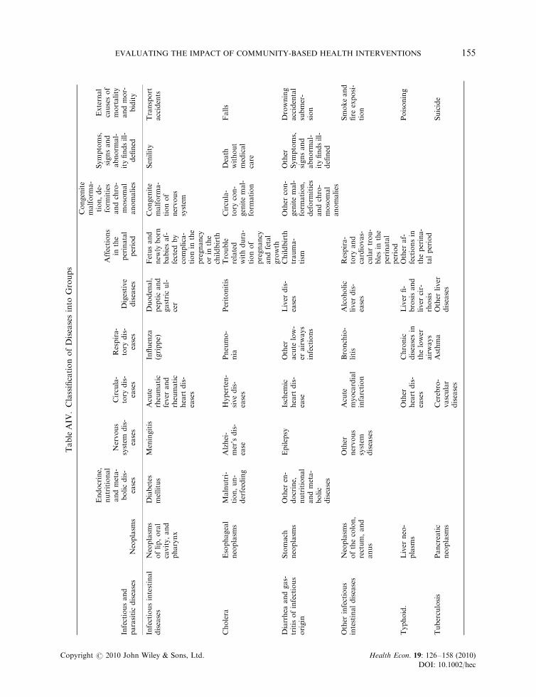
TableAIV

.ClassificationofDiseasesinto

Groups

Infectiousand

parasiticdiseases

Neoplasm

s

Endocrine,

nutritional

andmeta-

bolicdis-

eases

Nervous

system

dis-

eases

Circula-

tory

dis-

eases

Respira-

tory

dis-

eases

Digestive

diseases

Affections

inthe

perinatal

period

Congenite

malform

a-

tion,de-

form

ities

andchro-

mosomal

anomalies

Symptoms,

signsand

abnorm

al-

ityfindsill-

defined

External

causesof

mortality

andmor-

bidity

Infectiousintestinal

diseases

Neoplasm

soflip,oral

cavity,and

pharynx

Diabetes

mellitus

Meningitis

Acute

rheumatic

fever

and

rheumatic

heart

dis-

eases

Influenza

(grippe)

Duodenal,

pepticand

gastricul-

cer

Fetusand

new

lyborn

babiesaf-

fected

by

complica-

tionin

the

pregnancy

orin

the

childbirth

Congenite

malform

a-

tionof

nervous

system

Senility

Transport

accidents

Cholera

Esophageal

neoplasm

sMalnutri-

tion,un-

derfeeding

Alzhei-

mer’sdis-

ease

Hyperten-

sivedis-

eases

Pneumo-

nia

Peritonitis

Trouble

related

withdura-

tionof

pregnancy

andfetal

growth

Circula-

tory

con-

genitemal-

form

ation

Death

without

medical

care

Falls

Diarrhea

andgas-

tritisofinfectious

origin

Stomach

neoplasm

sOther

en-

docrine,

nutritional

andmeta-

bolic

diseases

Epilepsy

Ischem

icheart

dis-

ease

Other

acute

low-

erairways

infections

Liver

dis-

eases

Childbirth

trauma-

tism

Other

con-

genitemal-

form

ation,

deform

ities

andchro-

mosomal

anomalies

Other

Symptoms,

signsand

abnorm

al-

ityfindsill-

defined

Drowning

accidental

submer-

sion

Other

infectious

intestinaldiseases

Neoplasm

softhecolon,

rectum,and

anus

Other

nervous

system

diseases

Acute

myocardial

infarction

Bronchio-

litis

Alcoholic

liver

dis-

eases

Respira-

tory

and

cardiovas-

culartrou-

blesin

the

perinatal

period

Smokeand

fire

exposi-

tion

Typhoid.

Liver

neo-

plasm

sOther

heart

dis-

eases

Chronic

diseasesin

thelower

airways

Liver

fi-

brosisand

liver

cir-

rhosis

Other

af-

fectionsin

theperina-

talperiod

Poisoning

Tuberculosis

Pancreatic

neoplasm

sCerebro-

vascular

diseases

Asthma

Other

liver

diseases

Suicide



DOI: 10.1002/hec

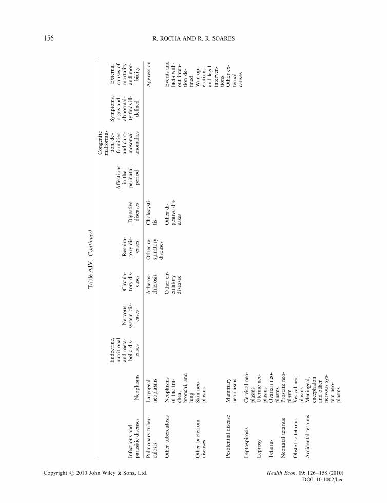
TableAIV

.Continued

Infectiousand

parasiticdiseases

Neoplasm

s

Endocrine,

nutritional

andmeta-

bolicdis-

eases

Nervous

system

dis-

eases

Circula-

tory

dis-

eases

Respira-

tory

dis-

eases

Digestive

diseases

Affections

inthe

perinatal

period

Congenite

malform

a-

tion,de-

form

ities

andchro-

mosomal

anomalies

Symptoms,

signsand

abnorm

al-

ityfindsill-

defined

External

causesof

mortality

andmor-

bidity

Pulm

onary

tuber-

culosis

Laryngeal

neoplasm

sAtheros-

chlerosis

Other

re-

spiratory

diseases

Cholecysti-

tis

Aggression

Other

tuberculosis

Neoplasm

softhetra-

chea,

bronchi,and

lung

Other

cir-

culatory

diseases

Other

di-

gestivedis-

eases

Events

and

factswith-

outinten-

tionde-

fined

Other

bacterium

diseases

Skin

neo-

plasm

sWarop-

erations

andlegal

interven-

tions

Pestilentialdisease

Mammary

neoplasm

sOther

ex-

ternal

causes

Leptospirosis

Cervicalneo-

plasm

sLeprosy

Uterineneo-

plasm

sTetanus

Ovarianneo-

plasm

sNeonataltetanus

Prostate

neo-

plasm

Obstetrictetanus

Vesicalneo-

plasm

sAccidentaltetanus

Meningeal,

encephalon

andother

nervoussys-

tem

neo-

plasm

s



DOI: 10.1002/hec

Diphtheria

Lymphoma

not-Hodgkin

Whoopingcough

Multiple

myelomeand

plasm

acell

neoplasm

sInfectiousmeningi-

tis

Leukem

ia

Septicemia

Benignneo-

plasm

Sexualdiseases

Other

neo-

plasm

sViraldiseases

Acute

poliomyelitis

Rabies

Dengue(breakbone

fever)

Yellow

fever

Other

viralfevers

Measles

Viralhepatitis

HIV

diseases

Protozoadiseases

Malaria

Leishmaniosis

Chagas’disease

Toxoplasm

osis

Helminthiasis

Schistosomiasis

Cysticercosis

Other

helminthiasis

Other

infectious

andparasitic

diseases



DOI: 10.1002/hec

The mortality effect of PSF by age group and interactions with early movers are given in Table AIII. Adetailed description of the specific causes of death included in each group is given in Table AIV.

REFERENCES

Aquino R, de Oliveira NF, Barreto ML. 2009. Impact of the Family Health Program on infant mortality inBrazilian Municipalities. American Journal of Public Health 99(1): 87–93.

Bertrand M, Duflo E, Mullainathan S. 2004. How much should we trust differences-in-differences estimates?Quarterly Journal of Economics 119(1): 249–275.

Bleakley H, Lange F. 2009. Chronic disease burden and the interaction of education, fertility, and growth. Reviewof Economics and Statistics 91(1): 52–65.

Bobonis GJ, Miguel E, Puri-Sharma C. 2006. Anemia and school participation. Journal of Human ResourcesXLI(4): 692–721.

Brazilian Ministry of Health. 2006a. Atenc- ao Basica e a Saude da Famılia. Ministerio da Saude – Brasil,Departamento de Atenc- ao Basica, Brasılia. Available from: http://dtr2004.saude.gov.br/dab/atencaobasica.php.

Brazilian Ministry of Health. 2006b. Saude da Famılia no Brasil: Uma Analise de Indicadores Selecionados,1998–2004. Serie C Projetos, Programas e Relatorios. Ministerio da Saude – Brasil, Brasılia.

Caldwell JC. 1986. Routes to low mortality in poor countries. Population and Development Review 12(2): 171–220.Fernandez M, Galiani S, Schargrodsky E. 2006. Targeted interventions in healthcare: the role of facility placement.

Fiscal Studies 27(3): 373–395.Fernandez-Val I. 2007. Fixed effects estimation of structural parameters and marginal effects in panel probit

models. Boston University, Unpublished manuscript.Fundac- ao Getulio Vargas and EPOS Health Consultants. 2001. ‘Determinac- ao e Avaliac- ao do Custo do Programa

de Saude da Famılia – PSF.’ Fundac- ao Getulio Vargas, Unpublished manuscript.Galiani S, Gertler PJ, Schargrodsky E. 2005. Water for life: the impact of the privatization of water services on child

mortality. Journal of Political Economy 113(1): 83–120.Kalemli-Ozcan S. 2002. Does mortality decline promote economic growth? Journal of Economic Growth 7: 411–439.Kalemli-Ozcan S. 2006. AIDS, reversal of the demographic transition and economic development: evidence from

Africa. NBER Working Paper No. 12181.Lleras-Muney A, Jayachandran S. 2009. Longevity and human capital investments: evidence from maternal

mortality declines in Sri Lanka. Quarterly Journal of Economics 124(1): 349–397.Lorentzen P, McMillan J, Wacziarg R. 2007. Death and Development. Journal of Economic Growth 13(2): 81–124.Macinko J, Almeida C, de Sa P. 2007. A rapid assessment methodology for the evaluation of primary care

organization and performance in Brazil. Health Policy and Planning 22(3): 167–177.Macinko J, Guanais F, de Fatima M, de Souza M. 2006. Evaluation of the impact of the family health program on

infant mortality in Brazil, 1990–2002. Journal of Epidemiology and Community Health 60(1): 13–19.Meltzer D. 1992. Mortality decline, the demographic transition and economic growth. Ph.D. Dissertation,

Department of Economics, University of Chicago.Miguel E, Kremer M. 2004. Worms: identifying impacts on education and health in the presence of externalities.

Econometrica 72(1): 159–217.Paes N, Albuquerque MEE. 1999. Avaliac- ao da Qualidade dos Dados Populacionais e Cobertura dos Registros de

Obitos para as Regioes Brasileiras. Revista de Saude Publica 33(1): 33–43.Riley JC. 2005. Poverty and Life Expectancy. Cambridge University Press: Cambridge.Riley JC. 2007. Low Income, Social Growth, and Good Health – A History of Twelve Countries. University of

California Press: Berkeley and Los Angeles.Rocha R, Soares RR. 2009. Evaluating the impact of community-based health interventions: evidence from Brazil’s

Family Health Program. IZA Discussion Paper No. 4119.Secretaria de Polıticas de Saude – Departamento de Atenc- ao Basica. 2000. Programa Saude da Famılia. Revista de

Saude Publica 34(3): 316–319.Soares RR. 2005. Mortality reductions, educational attainment, and fertility choice. American Economic Review

95(3): 580–601.Soares RR. 2007a. Health and the evolution of welfare across Brazilian municipalities. Journal of Development

Economics 84(2): 590–608.Soares RR. 2007b. On the determinants of mortality reductions in the developing world. Population and

Development Review 33(2): 247–287.Viscusi W, Aldy KJE. 2003. The value of a statistical life: a critical review of market estimates throughout the

world. Journal of Risk and Uncertainty 27(1): 5–76.



DOI: 10.1002/hec

poblacion 1

Documents

team of health

thefamily health program

form of health

health counseling

health outcomes

brazilian ministry of

provision ofbasic health

public health system