1

Staying Ahead and Getting Even: Risk Attitudes of Experienced Poker

Players

David Eil Jaimie W. Lien

George Mason University Tsinghua University Interdisciplinary Center for Economic Sciences School of Economics and Management

Version: March 19th, 2013

Abstract1

We study the behavior of frequent online poker players who have extensive experience calculating probabilities and expected values. Such players might be expected to behave as expected utility maximizers, in the sense that small shocks to their wealth would not change their risk preferences (Rabin, 2000). By contrast, the prediction of reference-dependent loss aversion (as in Prospect Theory) (Koszegi and Rabin, 2006; Kahneman and Tversky, 1979) is that risk aversion decreases as a player’s wealth travels away from the reference point in either direction. In terms of continuing to play, as well as via a more aggressive playing style, we find strong evidence for the break-even effect, the increased willingness to take on risk as a player is losing within a session. However, we do not find evidence for the house money effect, the increasing willingness to take on risk in the gains domain. Rather, experienced poker players’ behavior appears to be more consistent with existing evidence on reference-dependent labor supply, with players tending to reduce effort and risk-taking in response to being ahead. Taken together, our findings provide evidence for reference-dependent labor supply in a flexible, high-skilled setting, under conditions of well-understood monetary risk.

Keywords: Decision-making under uncertainty, reference-dependence, experience, risk JEL classification: D81 1 deil@gmu.edu ; jwlien@sem.tsinghua.edu.cn ; We would like to thank Vincent Crawford and Julie Cullen for their generous advice throughout the implementation of this project. We are grateful to Nageeb Ali, James Andreoni, Michael Bauer, Micheal Croteau, Gordon Dahl, Uri Gneezy, Daniel Houser, Brad Humphreys, Ryan Lim, John List, Juanjuan Meng, Craig McKenzie, Paul Niehaus, Justin Rao, Raymond Sauer, Charles Sprenger, and Li Zhou for helpful conversations and encouragement. We also thank participants at the Workshop on Gambling Economics at University of Alberta, Edmonton, and the Workshop in Behavioral and Decision Sciences at Nanyang Technological University. The UCSD Institute for Applied Economics and Tsinghua University provided research funding support. All errors are our own.

2

Introduction

The shape of an individual’s utility of money function is an important determinant of economic behavior across many domains. Neoclassical utility of money functions take only the decision maker's final wealth states as inputs – so the marginal utility of an extra dollar is fully determined by how much wealth the decision maker currently possesses, but not the amounts he may have possessed in the past, or the amounts he could have possessed in the present in different states of the world.

This assumption has implications for a myriad of important economic decisions, including those explicitly or implicitly involving risk, such as labor supply choices. A prediction of the neoclassical model is that wealth shocks that are small relative to lifetime income should have no effect on an individual’s risk aversion. By contrast, the main competing model, reference-dependent loss aversion (Koszegi and Rabin, 2006; Kahneman and Tversky, 1979), does predict that risk preferences are affected by small changes in wealth, and in a particular pattern: individuals become relatively more willing to accept risk after outcomes which move total outcomes away from their reference point, in either direction.

In this paper we study the behavior of experienced and on-average successful online poker players in order to test whether reference-dependence persists under expertise and well-developed knowledge of probabilities. Individuals in our sample play regularly and earn money doing so - on average, they play about 10 hours a week and earn nearly $40 per hour, typically playing several tables at once. We find that although the amounts of money won and lost within a sitting are small compared to their lifetime wealth, these transitory gains and losses do significantly affect their propensity to take on risk.

We document these patterns using two different measures of a player’s willingness to take risk. First, we estimate a player’s likelihood of continuing to play. Presuming that whatever activity they would do instead involves less risk than playing poker, continuing to play represents more risk-loving preferences than does discontinuing play. Second, we estimate a player’s likelihood of folding without putting any money into the pot in a given hand. Folding incurs a certain payoff while not folding induces some distribution of monetary outcomes. Therefore we consider not folding to be representative of more risk-loving preferences than folding.

In a manner consistent with reference-dependent loss aversion, players indeed exhibit a “break-even effect”, in which losses make them more risk-loving. This result is consistent with other evidence from the effect of shocks on risk preferences. For example, Post, Van den Assem, Baltussen and Thaler (2008) considers the behavior of contestants on the game show Deal or No Deal, in which contestants make a series of decisions under uncertainty. They find that “losers” in the game, who have been unluckier than the average contestant, are less risk averse than “neutral” contestants.

Post et al also find that, again consistent with loss aversion, “winners”, who have been luckier than average, are also somewhat less risk averse, but the effect is smaller. This is the “house money effect”, wherein individuals become relatively less risk averse the more money they win. However we find that experienced poker players do not generally exhibit the house money effect. Instead, we find that gains actually make players more conservative. This lack of house-money effect is robust to specifying the reference point as individual expected winnings as proposed by Koszegi and Rabin (2006).

Fundamentally, risk preferences are determined by an individual's valuation of a dollar gained relative to a dollar lost. A closely related choice is that of labor supply, in which an individual trades dollars gained not against dollars lost, but against costly effort. Since we study a player’s willingness to continue playing, we are

3

considering the valuation of dollars gained against both the valuation of dollars lost and the expenditure of effort. In this sense, decisions on how long to play resemble a labor supply choice, at least for skilled players, for whom expected profits are positive. The literature on labor supply in response to wage shocks is thus also closely related to our question.

Using detailed data on taxicab trip records, Camerer, Babcock, Loewenstein and Thaler (1997), as well as Crawford and Meng (2011) find evidence for daily income (and hours) targeting among drivers, a labor supply behavior which can be accounted for with reference-dependence, but not neoclassical life-cycle labor supply models. Fehr and Goette (2007) run a field experiment on bicycle messengers, testing whether they reduce effort in response to a positive transitory shock to wages. They find that reduced effort is prevalent and correlated with laboratory-style measures of loss aversion. In earlier literature, Dunn (1996) finds survey evidence for loss aversion among different worker types by tracing income-leisure indifference curves. Rizzo and Zeckhauser (2003) find evidence for loss aversion among physicians, by using survey responses regarding adequate income as the reference point.

A main contribution of our study is to the literature that studies differences in levels of loss aversion between novices and experts. List (2003, 2004) has presented evidence that reference dependent behavior is not exhibited by “experts”, and goes away with marketplace experience. List found that professional card dealers were less likely than novice card show attendees to exhibit the endowment effect, often explained as an artifact of loss aversion, drawing into question whether empirical evidence from laboratory experiments carries over to settings in which decision-makers are experts. Koszegi and Rabin (2006) show that this could result not from different degrees of loss aversion, but different expectations - in the case of List's “experts”, they expect to sell the things they get. Therefore selling the good does not feel like a loss to them, since they never expected to keep it. Crawford and Meng (2011) also find less loss aversion among the more experienced cab drivers in their sample. Pope and Schweitzer (2011) document evidence of loss aversion in professional PGA tour golfers. Our data comes from experienced and successful players playing with large stakes. On average, they play 300 hours over the seven months of our data, and earn almost $40 an hour. Moreover, the expected value calculations required to make profitable decisions as a successful player give them the computational skills knowledge of probability needed to make rational decisions. Yet, we still find that daily profits have a significant impact on their decisions.

Our study also offers a detailed analysis the dynamics of risk preferences in a white-collar, high skilled setting.2 Studying risk-taking behavior in a white-collar setting is a potentially important addition to the current existing literature, due to the possibility that there may exist certain features of previously considered physical labor settings which could make them more ‘prone’ to reference-dependence. For example, the risk associated with continuing past one’s reference point may increase in a particularly unappealing manner in the case of manual labor settings such as driving or construction, due to safety concerns and human physical limitations. In such occupations there may be a prevalent philosophy of “not working more than you have to” just for the sake of money. When individuals continue to play online poker, the risk players perceive due to any decrease in performance or concentration towards the task at hand, is monetary rather than physical.3

A further advantage of online poker is that for profitable players, it is a method of earning money with no

2 See Levitt and Miles (2011) which investigates whether poker is primarily a game of luck or skill, and finds strong empirical evidence that poker is a game of skill. 3 The different nature of demands on workers employed in manual or physically intensive labor versus computer and desk work is recognized and reflected in the exemption rules of the Fair Labor Standards Act.

4

explicitly imposed constraints on working hours, and no fixed costs of working on a daily basis.4 No certification or training is required – so in order to survive at this ‘job’ in the long run, players need to develop or research into their own strategies on when to stop, since they receive no official education on this matter. Thus we believe what we observe in online poker players’ behavior is really their natural response to their prior outcomes, and not any artifact of institutional constraints or advice. With substantial numbers of people working at home or taking on entrepreneurial projects with various associated risks on their own free time, our results may be indicative of the risk attitudes and behaviors of workers in other freelance labor supply settings.5

A study which is close to ours in terms of the nature of the work examined is Coval and Shumway (2005) which finds evidence of loss aversion among proprietary traders at the Chicago Board of Trade (CBOT). Like financial markets traders, individuals who regularly play poker for real money are well-versed in dealing with risk, and have demonstrated competence in numeracy and probability. Poker players, however, have the advantage of never seeing their market close. Tables stay open 24 hours a day, 7 days a week. In addition, the impact of winning and losing on future outcomes is less of a confounding factor in poker than in trading. The most obvious hypothesis in the case of poker is that earnings would be positively auto-correlated – losing early in the day predicts losing later in the day. This would suggest that players should quit earlier and fold more when they’re losing, which would be the opposite of what we find. Also, we can remove at least one source of auto-correlation in earnings by examining the effect on earnings at the nth table of earnings at the other n-1 tables. As shown in Section 5, this analysis does not change our estimates at all, indicating that the change in behavior is coming from the utility function, not beliefs.

We are not the first to look at the game of poker to detect evidence for the break-even and house money effects. Smith, Levere and Kurtzman (2009) use high stakes online poker data to evaluate playing style before and after particularly large wins and losses, and comparing what other possible behavioral biases might account for player behavior. They restrict their analysis to aggressive versus conservative playing style within particular hands, rather than overall playing time behavior, and focus on data from a high stakes level. Our findings are consistent with theirs in that they find players are less conservative and more aggressive in their play after losing an especially large pot, while becoming more conservative and passive after winning an especially large pot. While they take this as concrete evidence of the break-even effect, they refrain from speculating or investigating in detail about the lack of house money effect. Combined with recent progress in the literature on reference-dependent labor supply, by examining when players choose to end poker playing sessions, our findings suggest a possible labor-supply reason why Smith et al (2009) did not find much of a house money effect in the playing style domain. In Section 5, we replicate their main findings on our data using probit analysis.

Throughout our analysis, we will be treating player choices as decision problems, rather than strategic problems. Of course poker is a strategic game, and it is possible that what we are observing is part of a strategy designed to increase long-term winnings rather than changing risk preferences. It is also possible that

4 One can imagine online poker as a marketplace for experience, in which one type of player (leisure type) participates primarily for the leisure utility of playing, and is willing to pay a cost for the experience of doing so. Another type of player (profitable type) participates primarily to earn money through the losses of leisure players, while supplying playing experience to leisure players. Thus, while online poker may not be considered a conventional labor market per se, transactions analogous to a labor market setting take place indirectly. 5 Some examples could include selling items on Ebay or other online customer-to-customer retail sites, day trading in the financial markets, or individuals utilizing particular personal skills such as arts, teaching or programming to earn money on a job-by-job basis.

5

behavior reflects a belief in changes in others’ risk preferences, even while no player’s preferences actually change.

We have several justifications for this strategy. First, as we will discuss, the player pool is quite large, and players play on many tables at once. This means that executing a negative expected-value strategy early on in hopes of creating a bigger positive expected-value strategy later on against that same player is risky, since the chances of playing a big pot against that player are relatively small. Other players at the table can observe play, but given that most of them play multiple tables, they are unlikely to concentrate closely on hands in which they are not themselves involved. Second, while the equilibrium for this type of poker is not known and even if it were we would not expect all players to follow it, a strategy of giving up money early to win back more money later would be out of equilibrium.

Most importantly, we see no signs of this behavior in the data. Player performance does not seem to depend on previous winnings in the same session, although this data is quite noisy. In our probit analysis in Section 5, we also include in our regressions control variables such as stack size and number of players that could be important strategically. We also find that all types of winnings affect risk preferences equally. As discussed in Section 5.1, both winnings from “luck” (which cannot result from strategy) and “skill” (which might) affect risk preferences in the same way. If what we consider changes were actually a strategic decision, we would instead find effects only for winnings from “skill”. Finally, as discussed at the end of Section 5, winnings from the other n-1 tables have an effect on a player’s actions at a given nth table. Since players at table n will observe the protagonist’s actions at the other n-1 tables only very rarely, there is little reason to believe this change in playing style would be an effective strategy. All of these facts are, however, fully consistent with changing risk preferences.

The remainder of the paper is organized as follows: Section 2 discusses loss aversion and its predictions for poker players' playing time and risk-taking behavior; Section 3 describes the data set used and player characteristics; Section 4 explains the empirical strategy and describes results concerning time spent playing as a function of net winnings relative to various reference points. Our specifications in this section include both individual-level and pooled estimates of a duration model. We also consider alternative specifications of the reference point as suggested by players’ expected winnings, and recent winnings. Section 5 details findings on how poker playing style changes with net winnings, an issue investigated for large stakes decisions in Smith, Levere and Kurtzman (2009). We use a probit approach, controlling for several relevant variables which we observe in the data, and compare our results to theirs; Section 6 estimates the costs of the break-even effect to the online poker players in our sample; Section 7 concludes.

2. Prospect Theory

As discussed above, prospect theory specifies a value function that takes as its argument not the final wealth state of the individual, but a change relative to a reference point. Koszegi and Rabin (2007) write down the following utility function for money which combines both “consumption utility” and “gain-loss utility”:

U(x) = m(x) + μ(m(x)-m(r))

where x is some certain wealth outcome and r is the reference point. A commonly used special case is for m(x) to be linear. In fact, for amounts of a few hundred dollars, as discussed above, it must be the case that m(x) is linear.

A common specification for the gain-loss utility “value function” μ is as follows:

6

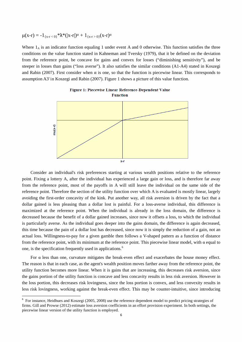
μ(x-r) = -1{x-r < 0}*λ*(|x-r|)α + 1{x-r > 0}(x-r)α

Where 1A is an indicator function equaling 1 under event A and 0 otherwise. This function satisfies the three conditions on the value function stated in Kahneman and Tversky (1979), that it be defined on the deviation from the reference point, be concave for gains and convex for losses (“diminishing sensitivity”), and be steeper in losses than gains (“loss averse”). It also satisfies the similar conditions (A1-A4) stated in Koszegi and Rabin (2007). First consider when α is one, so that the function is piecewise linear. This corresponds to assumption A3' in Koszegi and Rabin (2007). Figure 1 shows a picture of this value function.

Consider an individual's risk preferences starting at various wealth positions relative to the reference point. Fixing a lottery A, after the individual has experienced a large gain or loss, and is therefore far away from the reference point, most of the payoffs in A will still leave the individual on the same side of the reference point. Therefore the section of the utility function over which A is evaluated is mostly linear, largely avoiding the first-order concavity of the kink. Put another way, all risk aversion is driven by the fact that a dollar gained is less pleasing than a dollar lost is painful. For a loss-averse individual, this difference is maximized at the reference point. When the individual is already in the loss domain, the difference is decreased because the benefit of a dollar gained increases, since now it offsets a loss, to which the individual is particularly averse. As the individual goes deeper into the gains domain, the difference is again decreased, this time because the pain of a dollar lost has decreased, since now it is simply the reduction of a gain, not an actual loss. Willingness-to-pay for a given gamble then follows a V-shaped pattern as a function of distance from the reference point, with its minimum at the reference point. This piecewise linear model, with α equal to one, is the specification frequently used in applications.6

For α less than one, curvature mitigates the break-even effect and exacerbates the house money effect. The reason is that in each case, as the agent's wealth position moves farther away from the reference point, the utility function becomes more linear. When it is gains that are increasing, this decreases risk aversion, since the gains portion of the utility function is concave and less concavity results in less risk aversion. However in the loss portion, this decreases risk lovingness, since the loss portion is convex, and less convexity results in less risk lovingness, working against the break-even effect. This may be counter-intuitive, since introducing

6 For instance, Heidhues and Koszegi (2005, 2008) use the reference dependent model to predict pricing strategies of firms. Gill and Prowse (2012) estimate loss aversion coefficients in an effort provision experiment. In both settings, the piecewise linear version of the utility function is employed.

7

concavity in gains creates more risk aversion in gains, and convexity in losses introduces risk lovingness in losses. However this is only relevant for comparing gains to losses. That is, for α < 1, an individual will be more risk-loving after losing $100 than after winning $100. However, compared to α=1, an individual with α<1 would have a smaller decrease in risk aversion when moving from $100 to $200 in losses, and a bigger decrease in risk aversion when moving from $100 to $200 in gains.

In their original outline of reference dependent preferences, Kahneman and Tversky were (perhaps deliberately) vague about what the reference point might be. Candidates include the status quo, expected values, or the outcomes of others. Koszegi and Rabin (2007) specifies that the reference point should be the individual's “recent beliefs”. In our analysis, we will start out by assuming that a player's reference point is their wealth at the start of their session, so that session profits are exactly equal to deviation from the reference point. However we will also try relaxing that by allowing the reference point to equal their wealth plus the amount that they win in an average session.

A related question is the length of time before a change in wealth becomes internalized, and becomes the new reference point. When does the house's money become the gambler's own? This length of time is referred to as the “bracket” of an individual's decision. Once the bracket has closed, any gains are losses are internalized. While within the bracket, the individual can gain money to offset a loss before “booking” it, and likewise lose money to offset a gain.

Here we will start with an assumption that the player's bracket is at the session level. That is, the player starts every session in a new bracket, but is not forced to “book” gains or losses mentally until the session ends. For example, if a player loses $200 in the first hour of play and then makes $400, he will code this as a gain of $200. By contrast, if he loses $200 in one hour, quits, and comes back the next day and makes $400 in an hour, at that point he will consider himself to be up $400.

We can use the reference dependent model to inform our thinking about a poker player's decisions. First, let us consider a player's decision of how long to play. At each point in time, players face a decision of whether to end their session or continue playing. If they continue playing, they may gain some utility from playing itself (i.e., unaffected by the amount won or lost in the hand), and pay some cost in the effort required to make the best decisions possible. They also gain or lose utility based on the money that they win or lose from the game. In particular, consider a player who has played t minutes and is considering whether or not to continue for another dt. If he stops, he will have a utility of:

∫ −=t

tcdsswUtwV000 ))()(,(),( π (1)

where U(w,π) represents the players utility of wealth function, w0 represents the player's initial wealth, π(t) represents the player's profits in time t, and c(t) represents a combination of the positive utility from gambling and the effort cost paid to play the game, which are both assumed independent of the amount won or

lost in the session. For what follows, we will simplify notation by using Π(t) to denote ∫t

dss0

)(π , the

cumulative session profits up until time t, while still using the lowercase π(t) to refer to the profits arriving at time t. If instead he continues to play an additional dt minutes, he will have a expected utility of:

∫+

+−+Π=+dtt

tdttcdzztwUEdttwV )()])()(,([),( 00 π (2)

Whether V(w0,t) or V(w0,t + dt) is higher depends on the cost of additional effort, the distribution of

8

profits the player faces in the next dt minutes, and the marginal utility of these gains and losses. Clearly the player continues if (2) - (1) is positive, and stops otherwise. We will assume that the marginal cost of effort is increasing over at least some range, so that the player always stops eventually, and that it is separable from the utility of money.

This same model can be used to think about the player's decision to fold or not. Folding guarantees a profit of zero.7 Continuing in the hand, either by raising or by calling, gives the player some distribution of profits.8

We will be interested in the effect of session profits up until time t, Π(t), on these decisions. Due to Rabin's calibration theorem, we can consider the neoclassical expected utility case to be one where utility is linear in the amounts of money under consideration. In this case, (2) - (1) reduces

to

Continuing may also give the player some fixed utility from gambling, and require some cost in making further decisions in later betting rounds, again both captured by c(t).

∫+

−+−dtt

ttcdttcdssE ))()((])([ π .9

Now consider the predictions of prospect theory, using the piecewise linear value function specified above. We will start off by considering the reference point to be the individual's wealth going into the session, w0. Then (2) - (1) > 0 reduces to:

Π(t), the amount earned up until time $t$ in the session, can enter this

expression solely through its effect on beliefs regarding profits over the rest of the session. In absence of any such effect, we should expect expected utility maximizers to exhibit no systematic effect of session winnings on continuation probability.

+Π−>+Π⋅

Π−> ∫ ∫∫

+ ++ dtt

t

dtt

t

dtt

ttdzzdzztEtdzzP )]()(|)()([)()( πππ

−Π−<+Π⋅

Π−<⋅ ∫ ∫∫

+ ++)]()(|)()([)()( tdzzdzztEtdzzP

dtt

t

dtt

t

dtt

tπππλ

)()())(1)(1( }0)({}0)({ tcdttctt tt −+>Π⋅+Π <Π>Π λ (3)

where P(A) represents the probability of event A occurring. Let H(Π(t)) represent the LHS of (3). The top two lines show the expected utility from taking the risky option, divided into two parts: the top line represents the part of expected utility that comes from the gains. The second line represents the part that comes from losses. The bottom line subtracts off the opportunity cost, or the utility value of not taking the gamble. H(Π(t)) is then compared to c(t + dt)-c(t), the marginal effort of taking the gamble. This framework allows us to evaluate risk preferences at different values of Π(t). Recall that the player accepts the gamble whenever H(Π(t)) > c(t + dt)-c(t) and otherwise takes the fixed amount (either by folding or leaving the table, depending on the decision problem considered). Since the right hand side is independent of H(Π(t)) for a given session length, a higher

7 Unless the player is in one of the blinds, in which case folding guarantees a loss of the amount of the blind. 8 Clearly this distribution is conditional on the cards the player is dealt. But since the distribution of these cards is independent of Π(t), there is no reason to believe that the cards would somehow dictate that a player should be more or less likely to fold based on Π(t). 9 Strictly speaking, here we have set U(x) = x, which is more restrictive than linearity. However, for any linear utility

function )(ˆ xU , we can create a cost function )(ˆ tc such that

∫∫++

+−+Π=+−+Π+dtt

t

dtt

tdttcdsstwUEdttcdsstwE )(ˆ])()(,(ˆ[)(])()([ 00 ππ , so that there is no loss of

generality by simply assuming U(x) = x here.

9

H(Π(t)) means that the player is more likely to continue playing.

First let us consider H(0), evaluating the continuation decision when the individual is at the reference point:

∫ ∫∫+ ++

+>⋅

>=

dtt

t

dtt

t

dtt

tdzzdzzEdzzPH ]0)(|)([0)()0( πππ

∫ ∫∫+ ++

<⋅

<⋅

dtt

t

dtt

t

dtt

tdzzdzzEdzzP ]0)(|)([0)( πππλ

If H(0) > c(t + dt)-c(t), it must be that either ∫+dtt

tdzzE ])([ π is much greater than zero, so much so that it

would be positive even when the losses are weighted twice as heavily as the gains, or c'(t) < 0. Now consider

when Π(t) is much less than zero, some value Π(t), so much so that

Π−>∫

+dtt

ttdzzP ))()(π is zero. Then

H(Π(t)) reduces to:

)(])()([))(( tdzztEtHdtt

tΠ⋅−+Π⋅=Π ∫

+λπλ

∫+

⋅=dtt

tdzzE ])([ πλ

Clearly H(Π(t))>H(0), since

∫ ∫ ∫+ + +

>⋅>⋅−+=Πdtt

t

dtt

t

dtt

tdzzdzzEdzzPHtH ]0)(|)([)0)(()1()0())(( πππλ . This is the

“break-even effect”, that when the individual is far below her reference point, she is more likely to engage in risky action (here, H(Π(t)) is more likely to be above c(t + dt)-c(t)) than when she is at the reference point.

Finally, consider the case when Π(t) is much greater than zero at some value )(tΠ , so that

))()((∫ Π−<dt

ttdzzP π is zero. Then ))(( tH Π reduces to simply ∫

+dtt

tdzzE ])([ π . Again, this is greater

than H(0), since ∫ ∫ ∫+ + +

<⋅<⋅−+=Πdtt

t

dtt

t

dtt

tdzzdzzEdzzPHtH ]0)(|)([)0)(()1()0())(( πππλ . This

represents the “house money effect” - the individual is more likely to accept a given gamble when above her reference point than when at it. We have given the intuition for the break-even and house money effects by comparing extreme cases, comparing very high and low Π(t) to Π(t)=0. In general, a loss averse individual's marginal utility from taking a given gamble is a function of the probability with which they cross the reference point and the amount by which it is crossed. For gambles that are approximately symmetric around zero, such as the distribution of profits from a given hand, this is a function of the distance between Π(t) and the reference point.

We can also see that ))(())(( tHtH Π>Π as long as expected profits are positive. This reflects the fact

that the marginal utility of money relative to effort is higher in the loss portion than in the gain portion of the value function. Figure 2 summarizes these effect by graphing H(Π(t)) where dt is set to be long enough to play exactly one hand. For illustrative purposes, we have used for this graph the distribution of profits for just one

10

player in our data and assumed λ=2.The graph would look qualitatively similar regardless of which player's hands we had used, and any λ>1, as the differences in the distribution of profits for a given hand are relatively small across players.

Figure 2: Example: Expected Utility Gain for earnings from one hand (Player 12)

Figure 2 shows the amount of effort, in utils, that the player would be willing to expend in order to draw the profits from a random hand. Figure 2 (dashed line) also shows the same relationship under a non-linear μ with diminishing sensitivity, i.e., α < 1. We see the same V-shaped pattern of risk preferences, but with some difference in the slopes. Diminishing sensitivity increases the left-hand side derivative at zero, break-even effect for small losses, since the convexity in losses creates risk-lovingness. However it causes the break-even effect to decline at a faster rate, as the value function is becoming less and less convex as losses mount.10

We could also consider the reference point to be starting wealth plus the amount that the player expects to win when they sit down, as in the KR model. In this case, the player's risk aversion would increase with their session profits until they got to their expected winnings, at which point they would then start to decrease. That is, the graph above would just shift to the right, placing the minimum at expected winnings instead of at zero.

Conversely for gains, the decrease in risk aversion is initially smaller than in the linear case, so the right-hand side derivative at zero is smaller. This is because more of the gamble is covered by the concave gains portion of the value function and not the convex losses portion. However farther out in the gains domain, the house money effect is enhanced, so that H(Π(x)) has a second derivative closer to zero. This is a result of the individual moving to a more linear section of the value function.

3. Our Data Set

Our data consists of 9,120,559 No Limit Hold 'Em poker hands played online on the Full Tilt Poker site played between March and September 2009.11

10 For large enough losses, the slope can turn positive, so that more losses make the individual more risk averse.

All of these hands were played at cash tables with blinds of $2

11 Full Tilt is one of the two large online sites which accept US players, the other being Poker Stars. We used Full Tilt because gathering data is easier on this site. Although Full Tilt was one of several major online poker companies to have their gambling license temporarily revoked in late 2011, this did not affect the gathering or accuracy of our dataset which was collected two years prior.

11

and $4, with a maximum of nine possible players seated at the table. 12, 13, 14

The amounts of money being won and lost at the $2/$4 level are significant enough that the best players could use their winnings as their sole source of income. The mean hourly profit among our players is $39.06. While $2 and $4 may sound like trivial amounts, the amount of variance each player faces is substantial due to the unlimited betting structure of No Limit Hold 'Em. Even though the pot starts relatively small with just $6, hands in which over $500 transfers from one player to another are not uncommon. Furthermore, players are able to play many tables at once in order to increase their productivity. Players in our sample typically play between six and twelve tables at once. Thus the hourly variance in winnings is quite large. The mean standard deviation in winnings is $22.80 per hand. Since player play hundreds of hands per hour, this translates to an average hourly standard deviation of $570.67.

Our data set includes approximately sixty percent of all nine-player-maximum, $2/$4 Hold 'Em hands played on Full Tilt during this time period.15

We acquired our data from a site that collected it for the purpose of selling it to players. Because of server space limitations of this site, they gathered only about sixty percent of the total hands played during this time period. The main effect of missing forty percent of the data is to create attenuation bias, so that the estimates we present here act as a lower bound on the effects we describe (Li and Ryan, 2004). Our data follows a given subset of tables continuously, and then randomly switches to another subset, independently of the winnings of the players in the sample. Given the number of tables typically running at once at the $2/$4 stakes level, and the number of tables being played at a time by high-frequency players, the chance of a high-frequency player playing a session that is nowhere in our data is very low. However, since at any given time we only observe some fraction of the hands played by a given player, we do get a noisy estimate of that player's winnings. This noise biases our coefficient estimates towards zero.

We conduct our analysis on the 100 players within this sample who played the most number of hands. The first reason for our sample selection is practical, in that these are the players on whom we certainly have enough data to do an individual-level analysis. Furthermore, these are also the players who should be least likely to exhibit some kind of bias in their decision-making, since playing as often as they do, they can fairly be considered experts. The players in our sample are for the most part, making profitable decisions in their poker play. They also should have enough experience to know rules of basic probability, including calculating the probabilities of different cards being dealt, or the likelihood of another player holding a particular hand given their actions. Players committing systematic errors in calculations of this sort would be unlikely to remain profitable over the large time frame that we have covered in our data.

An advantage of using data from the $2/$4 tables is that stakes are small enough that there are many tables running all the time, so that there is no shortage of data to be gathered. This also means that the player pool is quite large, so that we have less worry that players are leaving the game due to other particularly bad players themselves entering and leaving. At larger games, this is quite common. For example, an entire $10/$20 game could start because one bad player sits down. Once that player leaves, all the rest of the players

12 Cash games are easier to analyze than tournament games, since in a cash game, a player who is risk neutral over money should also be risk neutral over chips. This is not necessarily the case in a tournament, for a number of reasons. 13 Blinds refer to the required bets that two players at the table must contribute in order to play the current hand - in this case $2 is the ``small blind” and $4 is the ``big blind”. Blinds rotate around the table so that each player takes turns contributing this required amount to the pot. 14 Typically the tables are full or close to full. The average number of players per hand was 8.1. 15 For Hold 'Em rules, see www.fulltiltpoker.com/holdem.php

12

will also leave, not wanting to play each other. At $2/$4, the ratio of regulars to casual players is much lower, so that the regulars can always find profitable tables should they want to play.

Full Tilt also hosts two-player and six-player maximum games, and a variety of different blind levels. $2/$4 is the highest blind level at which there are many tables running around the clock. The site also has other types of poker, such as Pot Limit Omaha and Limit Hold 'Em.16 However, players tend to play only one game and make it their “regular” game. Since we do not have comprehensive data from these other games, we cannot conclusively prove this to be the case using our data set. However conversations with online poker players, comments on online message boards, and aggregate player data from sites which monitor individual players suggest strongly that this is the case.17

Table 1 presents summary statistics on the most frequent 100 players in our data set. These are the players on whom we will focus all of our analysis.

The rationale is that there is an investment required to learn each type of game, including adapting to different styles of play at different stakes levels of the same game. As players experience long term gains or losses, they may decide to move up or down in stakes, but at a given point in time, they typically play just one class of game. This allows us to claim with confidence that the 100 players we use in our sample are $2/$4 No Limit Hold ‘Em regulars, and that when we observe a player to have stopped playing at the $2/$4 nine-person No Limit Hold 'Em tables, he has ended his poker-playing session.

As seen in Table 1, these players invested significant time in playing, with an average of over 300 hours over the course of 7 months. They were also rewarded handsomely for this effort, with an average hourly wage of nearly 40 dollars, or roughly twice the hourly wage an undergraduate could expect in an experimental lab. As such, these players are well-incentivized experts, capable of consistently making decisions that produce expected profits when analyzing risky choices.

4. The Break-Even Effect, “Locking in the Win” Effect, and the House Money Effect: Stopping Decisions 4.1 Correlation Coefficients

The principal finding of our analysis of stopping decisions is that a player's winnings in a session are negatively correlated with his likelihood of ending the session. That is, when he has lost money in the session, the more he has lost, the more likely he is to continue to play in an effort to get back to even (the “break-even effect”). When he has won money, the more he has won, the more likely he is to stop playing in order to “preserve the win”.

16 Limit Hold 'Em has the same structure as No Limit Hold 'Em, except that bets must be made in fixed increments. For Omaha rules see www.fulltiltpoker.com/omaha.php 17 See for instance www.pokertableratings.com. The other worry is that players may have multiple accounts, so that when ending a session under one screen name, they continue to play under another name. Again we cannot rule this out, but the site, as well as the poker community, strongly discourages this “multi-accounting”, and takes steps to prevent it.

13

For our analysis, we consider a session to have ended when a player does not play any poker hand for 6 hours consecutively. Although our choice of 6 hours as a precise cutoff point is arbitrary, we consider 6 hours a reasonable minimum interval of time after which players are likely to think of their playing as a “new session” once sitting down at the tables again. We have also run the analysis requiring a 10 hour break to “end” a session, with no qualitative impact on results. This is mainly because there are not very many breaks between 6 and 10 hours long. Players often take smaller breaks, in which they do not play a hand for fifteen minutes or an hour at a time. In these cases, for breaks longer than 5 minutes but less than six hours, we subtract the break time from the length of a player's session, but do not consider the session to have ended. So for example, if a player plays from 6:00 am to 9:00 am, then from 11:00 am to 1 pm, then from 10 pm to midnight, he has played two sessions, the first lasting five hours, the second lasting two hours. Our assumption, from a Prospect Theory point of view, is that the player “brackets” around each session. That is, he considers gains and losses within each session, then starts each session afresh at zero. His gain-loss utility in one session is therefore unaffected by his profits in an earlier session. In this sense, preferences are separable across sessions.

The first way we investigate the relationship between these gains and losses is by looking at the correlation between session length (in minutes) and session winnings. Since 96 of the 100 players in our sample are winning players (i.e., their total winnings are positive), if there were no relationship between a player's likelihood of quitting and their within-session winnings, we would expect the correlation between session winnings and session length to be positive. In fact, many of the players, even some of the biggest winners, have a negative correlation between session winnings and session length.

The average correlation across all 100 players is slightly positive, at 0.06. To evaluate whether this is more or less than one might expect if session stopping decisions were independent of winnings, we also calculated correlation coefficients using simulated data. To do this, for each player, we replaced the winnings from each hand with winnings from a hand drawn randomly from all of that particular player's hands. Because we sample from the entire distribution randomly while keeping the session lengths the same as in the actual data, the “quitting” decisions in our simulated data cannot be based on how much the player is up or down within the simulation.

Figure 3 shows a scatter plot of the mean of 1000 simulations for each player on the x-axis, along with the actual correlation coefficients found in the data on the y-axis. Most of the points lie below the 45-degree line in black, indicating that the correlation between session winnings and length in the data is lower than in the simulated data. The red line indicates the regression line. The constant is negative and statistically significant.

14

Fifteen players have correlation coefficients significantly less than their simulated values at the five

percent level, while only four have a correlation significantly above their simulated value. The average t-statistic across all 100 players is -0.42. The probability of drawing an average this far from zero on 100 draws from the standard normal distribution is 0.001%. This indicates either that players tend to continue their sessions longer when they are down and cut them short when they are up, or that players tend to do poorly when they play too long, or both. In the next subsection we show that it is the former effect that drives this result.

4.2 Cox Likelihood Analysis In order to analyze quitting decisions in more detail, we estimate a hazard model for each player. Utilized

frequently in the biomedical literature, hazard models have been previously utilized to model industry exit of new firms (Audretsch and Mahmood, 1995), employee attendance and absences (Johansson and Palme, 2005), and the effect of labor market programs on unemployment duration (Lalive, Van Ours and Zweimuller, 2008). Since we are interested in the effect of winnings on the likelihood of quitting more than any parametric relationship between time itself and quitting, we implement the Cox proportional hazard (Cox, 1972), which has the advantage that it does not require specifying an underlying hazard rate with respect to time, and is ideal for a primary interest in the relationship of the covariates to quitting than the hazard rate itself. We focus primarily on individual player-level estimates because we have sufficiently rich data, and to avoid concerns about unobserved individual heterogeneity (Elbers and Ridder, 1982 ; Heckman and Singer, 1984).

The Cox model allows for the effect of time on duration to be arbitrary, as long as we assume that it is multiplicative in the overall hazard function, and identical across sessions for a given player (note that since our regressions are at the individual player level, across-player heterogeneity is fully allowed). Given that our objective is to pick up directions of departure from the case of neoclassical expected utility model as a function of current wealth, we find this assumption reasonable for our purposes. Non-proportional hazard models on the other hand, require some specific assumptions about how the passing of time structurally affects the hazard rate (such as the frequently used Weibull distribution). We found these assumptions to be too stringent for our data, as we estimated significant coefficients using the simulated data described in the

15

previous section when none should have been found in theory. This lead us to conclude that the frequently used forms of parametric hazard function are likely misspecified in our context. The Cox model, by contrast, did not estimate significant coefficients in our random simulations, allowing confidence that effects detected in estimations using our actual data are real.

In order to construct the likelihood function, we order a player's sessions 1,2,...,n,...,N from shortest to longest. We have a vector of time-varying variables X(n,t) that we hypothesize affects the hazard rate of the session. Now let us suppose that session 1 ends at time T(1). Given that a session did end at time T(1), we can model the likelihood of session 1 being the session ending at that time as:

∑ =⋅⋅

⋅⋅N

nj nTj

nTn

TgX

TgX

))1(()exp(

))1(()exp(

)(,

)(,

β

β

The g(T(1)) function, which represents the effect that time has on the hazard rate (often modeled as a Weibull distribution in other applications) cancels, and we are left with just functions of the covariates of interest. While this allows us flexibility, the cost is loss of data. To see why, assume that the first session ends at t = 1 and the second session ends at t = 3. While we may have data on many sessions for t = 2, we are unable to conclude anything from these continuation decisions, since we cannot say if these decisions were due to effects from the covariates in X, or something to do with g(2), i.e., the effect of time. It could be that there is some strong impact to continue precisely at t = 2, which is independent of the covariates in X. As a result we have to essentially disregard all data from continuation decisions made at durations where no other session ends.18

The entire likelihood function for a player is constructed by multiplying the above ratios for each session we observe. Let Ti(s) be the length of session s for player i. Let Si be the total number of sessions played by player i. Let Πi,s,t be the winnings in session s for player i at time t. A player's entire likelihood function is then:

∏∑=

=

⋅

⋅=

i

i

i

iS

sS

sj isTji

isTsiii

X

XL

1 )(,,

)(,,

)exp(

)exp()(

β

ββ

Xs,t, the vector of independent variables, will vary according to the specification at hand, but in general will be some function of Πi,s,t. Notice that we estimate coefficients separately for every player. It is possible to estimate a kind of pooled Cox regression, where n would index all player sessions. However this would assume not only that the effect of time is proportional, but that it is uniform across players, which may not be a very realistic assumption. There is also considerable possibility of, and interest in, heterogeneity in the βi

coefficients, which is lost in a pooled regression. These facts, together with the computational difficulty of a pooled regression due to the amount of data, led us to working with the individual-level estimates. In Section 4.3 we address the possibility of classifying players by types. Thus the coefficients in βi will indicate how the different variables in Xs,t affect the likelihood of a session ending for player i.

Note that because our players are playing several tables at once, and we conduct the hazard analysis with time as the unit of observation, we cannot meaningfully control for table-level covariates such as stack size, position at the table, etc. We do however include these covariates of interest in our analysis of playing style at

18 In general when doing Cox likelihood regressions, one must worry about ties in durations. However since our data is at the seconds level, the time partitioning is fine enough such that we have no ties in lengths of sessions played by the same player.

16

the hands level in Section 5. Our standard errors are obtained via jackknife estimation, with omitted observations at the session level as implied by the Cox model.19

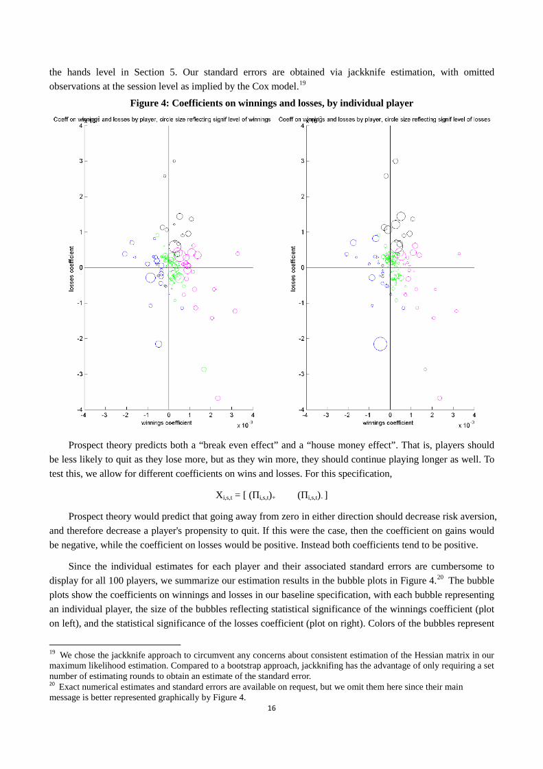
Figure 4: Coefficients on winnings and losses, by individual player

Prospect theory predicts both a “break even effect” and a “house money effect”. That is, players should

be less likely to quit as they lose more, but as they win more, they should continue playing longer as well. To test this, we allow for different coefficients on wins and losses. For this specification,

Xi,s,t = [ (Πi,s,t)+ (Πi,s,t)- ]

Prospect theory would predict that going away from zero in either direction should decrease risk aversion, and therefore decrease a player's propensity to quit. If this were the case, then the coefficient on gains would be negative, while the coefficient on losses would be positive. Instead both coefficients tend to be positive.

Since the individual estimates for each player and their associated standard errors are cumbersome to display for all 100 players, we summarize our estimation results in the bubble plots in Figure 4.20

19 We chose the jackknife approach to circumvent any concerns about consistent estimation of the Hessian matrix in our maximum likelihood estimation. Compared to a bootstrap approach, jackknifing has the advantage of only requiring a set number of estimating rounds to obtain an estimate of the standard error.

The bubble plots show the coefficients on winnings and losses in our baseline specification, with each bubble representing an individual player, the size of the bubbles reflecting statistical significance of the winnings coefficient (plot on left), and the statistical significance of the losses coefficient (plot on right). Colors of the bubbles represent

20 Exact numerical estimates and standard errors are available on request, but we omit them here since their main message is better represented graphically by Figure 4.

17

estimated classification groups, which we explain in detail in the next section (4.3).

Our primary result is that the likelihood of quitting tends to increase in the amount won so far in the session, regardless of whether the amount won is positive or negative. This can be seen in Figure 4 by the fact that most of the larger bubbles are concentrated in the upper right quadrant of the plots. The coefficient on losses is positive for 60 players, 32 of them statistically significant at the 5% level. The tendency towards positive coefficients is even stronger for gains. 67 players have a positive coefficient on gains, 35 of these significant. Thus, while we do see a “break even effect”, as Prospect Theory predicts, instead of a “house money effect”, where players gamble freely with “found money”, there is instead a “preserve the win” mentality, where once a player has won some money, he is more likely to quit and book a win, rather than continue playing and risk falling back to even or even possibly to a loss.

4.3 Classification Analysis

While the estimates from these individual-level regressions show a general tendency towards the house-money effect and a lock-in-the-win effect, there is clearly heterogeneity across the players. Another useful way of describing this heterogeneity is by creating different groups of behavioral types, forcing coefficients to be equal within each estimated type, and assigning each player to the group that best describes his behavior. We follow the approach of El Gamal and Grether (1990), which classifies individual belief updating processes using experimental data. When allowing for N classifications, we choose N parameter vectors such that:

))(ln(maxmax},...,,{100

1 },...,,{)(},...,,{

**2

*1

212

21ii

iN L

NiN

N

βββββββββββ

∑− ∈ℜ∈

=

Table 2 presents the data for 2, 3, and 4 group classifications:

When only two groups are allowed, the first exhibits both a break-even effect and a lock-in-the-win effect, the principal tendencies in the data we have been discussing. The second group exhibits a weaker break-even effect and a weak house-money effect, the standard pattern for loss-averse behavior.

Adding in a third group creates a category for players whose behavior is exactly contrary to the main tendency in the data. That is, for this categorization of players, winning tends to lead them to play longer, while losing leads them to quit sooner. This is the pattern one might expect from a player who understands results to be some kind of signal of their expected profits in future hands played in that session. These players are a minority, including only 22 of the 100 players. These 22 players come almost exclusively out of the “loss averse” category when only two groups are allowed. The population of this type drops from 61 to 42, whereas the population of the first group stays relatively constant (drops from 39 to 36). Also, when this category is

18

included, both of the other two categories now have two positive coefficients. This indicates that the “house money” behavior seen in the second type of players when only two classifications are allowed is being driven by these players who also quit sooner when behind. That is, these are not loss-averse types, who play longer the farther away from zero they are, but “past performance indicates future results” types, as described above. As a result, when three possible types are allowed, two of the three have all positive coefficients; these two categories cover 79 of the 100 players.

Finally, when four types are allowed, group 1, which featured large and approximately equal positive coefficients when two and three groups are allowed, breaks up into two groups, one in which the “lock in the win” effect is more pronounced (23 players), and another in which the “break-even effect” is more pronounced (13 players). The populations of the other two types are left unchanged. This analysis therefore suggests the same conclusions as the individual-level analysis: A minority of players are more likely to quit the more they lose, and more likely to continue the more they win. A majority of the players, in varying degrees, are more likely to continue the more they lose (the break-even effect), and more likely to quit the more they win (the lock in the win effect).

4.4 The Disproportionate Effect of Recent Profits

Although we have assumed so far that players “bracket” over sessions (i.e., they consider themselves to be a winner on a loser by comparing their current wealth to their wealth at the start of the session), it is possible for players to bracket over shorter lengths of time. Perhaps winnings from an hour or two earlier have already “sunk in”, so that if a player wins $400 in the first ten minutes of play, is even for the next hour, then loses $200, he considers himself to be down $200 rather than up $200.

To test this, we broke session winnings into all winnings and “recent” winnings, definedas winnings within the last ten minutes of play. For this specification, our vector of regressors is:

Xi,s,t = [ (Πi,s,t)+ (Πi,s,t)- (Πi,s,t -Πi,s,t-10)+ (Πi,s,t -Πi,s,t-10)-]

The results of this estimation suggest that many players are bracketing over more recent time frames, and that when this is accounted for, the coefficient signs are different for wins and losses, as prospect theory would predict. Specifically, the coefficient on recent gains is significantly negative for 31 players, while the coefficient on recent losses is significant for 29 players, showing a clear “break-even effect” and “house money effect” across many players. The pattern in the coefficients on profits for the entire session remain roughly the same as in our second specification, with 40 players having a significantly positive coefficient on session winnings, and 34 players having a significantly positive coefficient on session losses.

This is the only point in our analysis where we find any house money effect. It may be that the direction of causation is in fact reversed. The decision to stop is not made instantaneously and unexpectedly. It could be that the effect here is not that that higher recent winnings decrease the likelihood of a player stopping, but instead that once a player knows he will quit soon, he plays differently. In the next section we analyze player decisions once they are dealt in on a hand. This analysis does not suffer from this concern, and there we see no house money effect of recent winnings.

4.5 Expectations as Reference Point

One possible reason that we do not find the house money effect for session winnings is that we have set the reference point to zero. It would make sense, in the Koszegi-Rabin model of the reference point as rational expectation, for the reference point to be greater than zero. Since these are winning players, they make money

19

on average when they sit down to play. If this were the case, then more winnings should decrease the probability of quitting a session, but only once winnings get past a certain point. To test this model, we estimated another specification of the Cox model with:

])()[( ,,,,,, −+ Π−ΠΠ−Π= itsiitsitsiX

where iΠ represents the average profit per session for player i. Crawford and Meng (2011) take an analgous

approach in estimating the daily reference point for taxicab drivers. However the results still show that quitting probability increasing with session winnings is the more common pattern. 36 players have a significantly positive coefficient, while 15 players have significantly a negative coefficient on their session winnings over and above their average profits. Even when winning more than they would expect to win in an average session, more players try to lock in their win by quitting earlier than continue playing with the “house money”.

Table 3 summarizes the results from each regression:

5. The Effect of Profits on Playing Style

If session profits influence a player's willingness to continue playing by affecting his risk aversion, then playing style might also change in response to session profits. While playing style is difficult to summarize in one statistic, and can be influenced by many factors that are difficult to control for, the evidence tells the same story as the analysis of quitting decisions. Whereas up until this point we have been aggregating a given player’s explanatory variables over time intervals, in this section our unit of observation will be one hand played by one player.

The findings in this section build on the work of Smith, Levere and Kurtzman (2009). They investigate how the play of high stakes players changes following big wins and big losses.21

21 Their data comes from games with blinds of $25 and $50, 12.5 times the stakes in our data.

They find that individuals play both more loosely and more aggressively following big losses than following big wins. A complication, which brings difficulty to virtually any analysis of in-game decisions, is that it is difficult to attribute this difference definitively to a change in risk aversion, rather than a change in beliefs. That is, it could be that players believe that other players believe that they will play more conservatively following a big loss. Then their response of playing more recklessly following a big loss is a best-response given these beliefs and an

20

everywhere-linear utility function, rather than a result of unchanging beliefs about the actions of other players in conjunction with a loss-averse utility function.

Our data largely overcomes this difficulty, due to the fact that players in our dataset are playing at a lower stakes level and are thus playing many tables at once. Since they generally sit with many different players across their tables, it is unlikely that player j sitting at player i's first table will know for example, when player i just lost a big pot at his second table. Therefore if player i loses a big pot at one table and then plays more recklessly at all his tables, it is less likely to be his response to a belief that other players think he will be playing more conservatively following his big loss (since they most likely did not observe this loss), and more likely that his risk aversion has decreased. A further advantage of our analysis is that we include as many observable control variables as possible in our regression analysis for each individual player, while Smith, Levere, and Kurtzman (2009) restrict their analysis to signed-rank tests to look at differences in play before and after big hands.

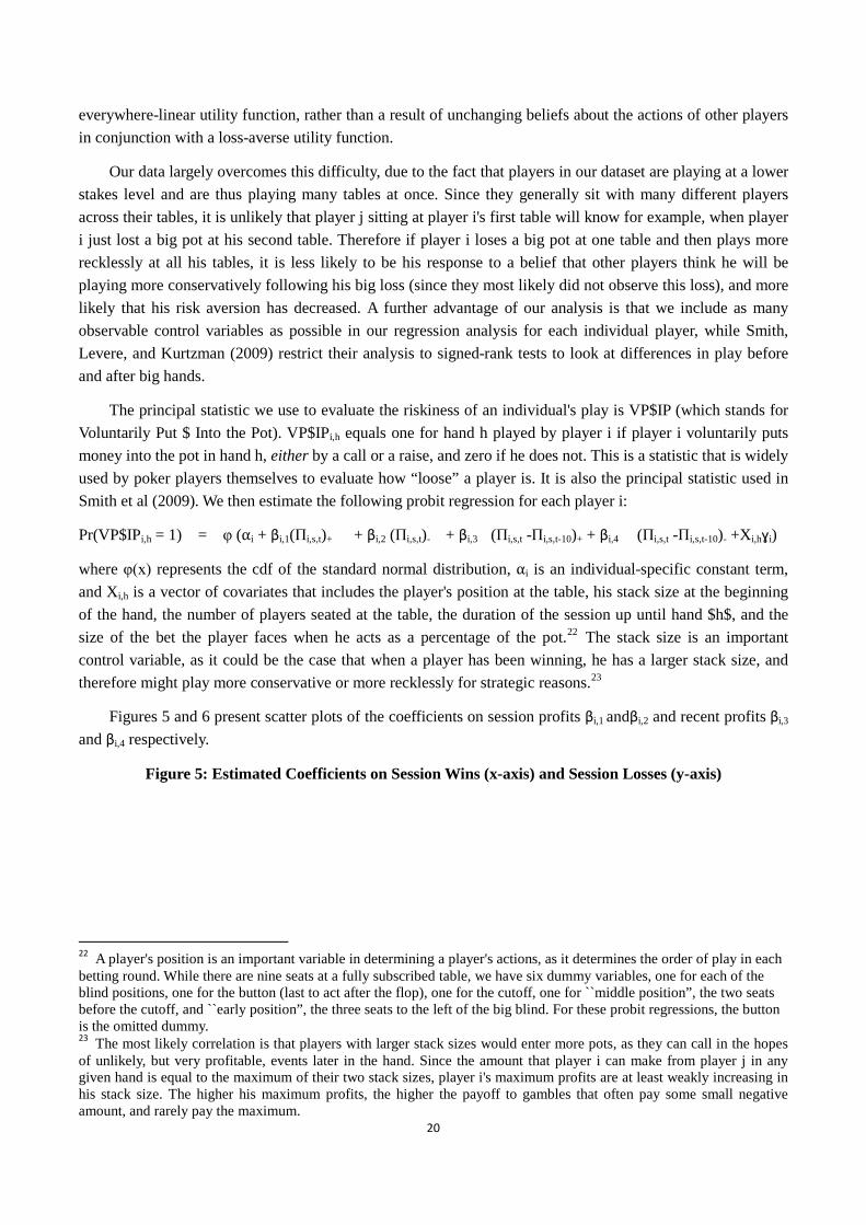
The principal statistic we use to evaluate the riskiness of an individual's play is VP$IP (which stands for Voluntarily Put $ Into the Pot). VP$IPi,h equals one for hand h played by player i if player i voluntarily puts money into the pot in hand h, either by a call or a raise, and zero if he does not. This is a statistic that is widely used by poker players themselves to evaluate how “loose” a player is. It is also the principal statistic used in Smith et al (2009). We then estimate the following probit regression for each player i:

Pr(VP$IPi,h = 1) = φ (αi + βi,1(Πi,s,t)+ + βi,2 (Πi,s,t)- + βi,3 (Πi,s,t -Πi,s,t-10)+ + βi,4 (Πi,s,t -Πi,s,t-10)- +Xi,hɣi)

where φ(x) represents the cdf of the standard normal distribution, αi is an individual-specific constant term, and Xi,h is a vector of covariates that includes the player's position at the table, his stack size at the beginning of the hand, the number of players seated at the table, the duration of the session up until hand $h$, and the size of the bet the player faces when he acts as a percentage of the pot.22 The stack size is an important control variable, as it could be the case that when a player has been winning, he has a larger stack size, and therefore might play more conservative or more recklessly for strategic reasons.23

Figures 5 and 6 present scatter plots of the coefficients on session profits βi,1 andβi,2 and recent profits βi,3 and βi,4 respectively.

Figure 5: Estimated Coefficients on Session Wins (x-axis) and Session Losses (y-axis)

22 A player's position is an important variable in determining a player's actions, as it determines the order of play in each betting round. While there are nine seats at a fully subscribed table, we have six dummy variables, one for each of the blind positions, one for the button (last to act after the flop), one for the cutoff, one for ``middle position”, the two seats before the cutoff, and ``early position”, the three seats to the left of the big blind. For these probit regressions, the button is the omitted dummy. 23 The most likely correlation is that players with larger stack sizes would enter more pots, as they can call in the hopes of unlikely, but very profitable, events later in the hand. Since the amount that player i can make from player j in any given hand is equal to the maximum of their two stack sizes, player i's maximum profits are at least weakly increasing in his stack size. The higher his maximum profits, the higher the payoff to gambles that often pay some small negative amount, and rarely pay the maximum.

21

Figure 6: Estimated Coefficients on Recent Wins (x-axis) and Recent Losses (y-axis)

Players generally play less conservatively as their session losses increase. 14 of the 100 players had coefficients on their session losses that were significantly negative at the 5% level. That is, as their losses mounted, they became more likely to enter future pots in hopes of recouping their losses. 17 players had significantly negative coefficients on their session gains. The more profits these players had in their session, the more conservatively they played, in order to protect the losses they had. Recent gains affected players more than gains at the beginning of the session, as 28 players had significantly negative coefficients on their recent winnings. Recent losses were more likely to be significant than earlier losses, as 21 players had a significantly negative coefficient on their recent losses. Recent gains and losses had a much stronger effect than overall session profits.

On average, players who have recently lost $400 are 0.54 percentage points more likely to enter a pot when in the dealer position, not facing a raise at a nine-handed table, an hour into their session, with no other gains or losses throughout the session.24

24 Being in the dealer position means that the player is last to act after the flop, a significant strategic advantage. It means nothing regarding the actual dealing of the cards.

Players who have recently won $400 in the same situation were on

22

average 0.66 percentage points less likely to enter the pot. However if the $400 had been won (lost) earlier in the session, the average decrease (increase) was only .10 (.03). It seems that players become more risk-loving following losses, and more risk-averse following gains, but much of the effect wears off fairly quickly.

As a robustness check, we also ran the same regression but included in Πi,s,t, the profits in the session up until time t, only hands from tables other than the table on which the hand played at time t was played. That is, if a player is playing at tables 1, 2, and 3, and we want to predict VP$IP for a hand at table 1, we take his cumulative winnings within that session at tables 2 and 3. This should remove any of the strategic effect discussed earlier, that even if players' risk preferences are not changing, they might believe that other players think they do, and this might change their play. The player pool is large enough that players do not generally share more than one or two tables with another player. Therefore winnings at other tables affect their play at a given table only through their risk preferences.

Consistently with the earlier results, players who have lost money, even at other tables, tend to play more loosely. Players who have won money tend to play more tightly. The estimates of the effects are lower, because of the fact that leaving out one table introduces more noise into the explanatory variable, creating additional attenuation bias. That is, it could be that the player is down at tables 2 and 3 but has won enough at table 1 to be up for the session overall. Still, of the 100 players, 15 of them had coefficients on their session losses significant at the 5% level, while 25 had significantly negative coefficients on their gains. The corresponding number of players with significantly positive coefficients was 8 and 3, respectively.

5.1 Luck versus Skill

As another robustness check, we can separate profits out into profits due entirely to luck, and profits due to some combination of luck and skill. In some hands, players will get all of their chips in the pot before the last card is revealed. In these cases we can see what all players' cards are, how much is in the pot, and therefore calculate what each player's expected earnings are at that point. Deviations from this expectation are due purely to luck, as there are no decisions to be made after all the chips have already been bet.25

If the observed behavior were due to a belief in mean reversion, there should be a stronger effect on the “pure luck” component of earnings. Table 4 presents the average coefficients on probit regressions that separate the winnings and losses on the right hand side into “pure luck” and “some luck, some skill” components.

We will call this part of profits “pure luck”, with the remainder being the “some luck, some skill” component.

25 As an example, say 1 player has a pair of aces against another player with a flush draw and they get their entire stack of $400 in the pot with one card to come. There are 44 cards left in the deck. Nine of them make a flush for the second player, giving him a

449 chance of winning the pot. This player's expected winnings at this point are

therefore 36.236$4435400$

449400$ −=− .

23

There is no statistical difference between the coefficients in any of the categories. This indicates that it is changes in risk attitudes and not beliefs in the gambler's fallacy that drives changes in behavior.

We also find some evidence suggesting that behavior is consistent across these two domains. There is a negative correlation across players (ρ = -.29) between the coefficient on gains in the Cox hazard estimation of stopping probability and the coefficient on gains in the probit regression predicting their likelihood of putting chips in the pot. Likewise there is also a negative correlation (ρ= -.07) between the coefficient on losses in predicting stopping probability, and the coefficient on losses in predicting VP$IP. That is, the players who are more likely to quit (continue) playing as they win (lose) more are also those more likely to play more conservatively (loosely). This indicates some consistency of risk preferences across the different choice domains.26

6. Cost of Loss Aversion

It seems intuitive that hand winnings would be serially correlated, since opponents are roughly constant within a session, as well as a player's state of mental awareness and focus. This would mean that continuing sessions in which one is losing, and cutting short more profitable sessions, would be a particularly bad strategy.

In fact, we find little evidence that winnings are serially correlated. This is partly because hand-by-hand profits are extremely noisy. In order to investigate the autocorrelation of session winnings, we estimate the following regression:

Πi,s,t -Πi,s,t-1 = αi + βi,1(Πi,s,t)+ + βi,2 (Πi,s,t)- +Xi,hɣi + єi,s,t

The left-hand side is then the winnings in the hand played at time t, while on the right-hand side is an individual fixed effect, the profits in session n up to, but not including, the hand whose profits are on the left-hand side, those profits squared, and a matrix of covariates including the session duration, the player's table position, stack size, and the number of players at the table.

The estimated β coefficients are estimated to be negative, indicating that players actually play better when they are losing, and worse when they are ahead, but the statistical relationship is weak, with average t-statistics of -0.057 for recent gains and -.114 for recent losses. On average, this means that an extra $100 in recent gains will decrease the expected winnings in a given hand by half a cent. The same increase in recent losses will increase expected profit per hand by about a cent.27

As a result, the cost of profit-dependent stopping strategies is negligible. Some instructional books advise that players should set a “stop-loss” in order to protect themselves from playing too long when they are losing, and potentially in an unprofitable situation. Since most of our players are winning players, even when they are playing poorly, they are still winners, just slightly less so. Therefore for a fair evaluation of this “stop-loss” strategy, we replace the hands that would have been un-played had by adding in simulated profits from additional sessions.

26 That the correlations are not stronger is not completely surprising. Not only is there some noise in these estimates, but risk preferences often vary significantly within individual behavior, even across similar simple tasks in experiments (Andersen, Harrison, Lau and Rutstrom, 2008). 27 There is some amount of negative bias in these estimates, so it is still possible that profits do have positive autocorrelation. The reason is that the left-hand side variable at time t feeds into the right-hand side at time t+1. In simulations we can see that this results in a β coefficient that is negatively biased, in approximately the same magnitude as the coefficients we estimate.

24

95 of the players had sessions in which they were down at least $800 at some point.28

7. Conclusion

Of these, 39 would have won more money using the stop-loss strategy, while 56 would have won less. Had they stopped at this point and instead played sessions later, on average they would have won $621 less. While not inconsequential, these players win and lose this amount in one hand with regularity. In fact, because of a positive correlation between the amount that a player would gain from a stop-loss strategy and their winnings, on average players would increase their winnings by 4.8% under a stop-loss strategy. Also, this calculation of cost does not take into account the extra variation in session length caused by conditioning stopping on profits. If the cost of their effort were a convex function of the amount of time they spent playing, it could be that this extra variance imposes substantial costs. There is also enough variance that the difference is not statistically significant. The t-statistic on the mean is -.997.

Strengthening the current evidence for loss aversion in the field, we find that even experienced and successful online poker players become less risk averse after sustaining losses. We observe this in our data through two domains of behavior: the decision to continue playing during losing sessions, and playing more recklessly following losses. The more money that the experienced and frequent players comprising our sample had lost, the less likely they were to end their poker session for the day, leaving them in a position of continued risk. Within individual hands dealt, they were also less likely to fold, thus exposing them to the risk associated with continuing in the hand. These are the typical break even effect results of loss aversion over monetary outcomes, and our analysis shows the prevalence of these behaviors among experts using field data.

Our findings question the hypothesis that experts can learn to correct loss aversion as a “bias”. This could be due to the fact that the expected monetary cost of this behavior is relatively low in our setting, in that our players do not play significantly worse as their losses mount. It may even be the case that some of these players are aware of their own bias, and still cannot overcome it. Instructional poker books counsel players to think of themselves as playing “one long session” over their entire career, as opposed to bracketing narrowly by thinking of each session separately (Hilger, 2007).

On the gains side, our results require more speculation in order to be interpreted. The players in our sample showed little evidence of the house money effect predicted by our proposed model of reference-dependent loss aversion over monetary outcomes. Rather players became significantly more conservative following wins, a type of “lock in the win” effect.

One possibility is a reference point updating story. We can imagine a model in which the reference point updates over time, but with insufficient adjustment compared to the case of lagged status quo. Since these players do earn money on average, a rational expectations model of reference dependence predicts that they should start with a positive reference point. Suppose that they update this reference point as the session progresses, but by an amount less than session profits. Then when a player wins, they update their reference point upwards, such that their wealth position remains below the reference point, but by a smaller amount than when they started. When they lose, their reference point adjusts downwards, but not by as much as they lose, so they end up farther away from the reference point. Recall that in the piecewise linear case, risk aversion is purely a function of distance from the reference point. Then such a process of updating the reference point would result in exactly the pattern we observe, that winning results in more risk aversion, while losing results

28 The 5 players who did not have such sessions are “shortstackers”, players who buy in for the minimum $80 at each table as opposed to the maximum $400.

25

in less. This is consistent with the intuition that for these frequent and successful players, they consider the money they win to be money “earned” through hard work and good decision-making, and which they value as soon as they receive it. This would be in contrast to the novice gambler in a casino, to whom a lucky streak brings unexpected money without a sense of entitlement to it – it is still “the house’s money”.

A further notable finding in our analysis is that the effects of wins and losses are rather transient, with profits in the most recent ten minutes having a much stronger effect than cumulative profits over entire sessions which generally last several hours. This suggests that individuals do bracket narrowly, and that developing a model of reference point updating is important in applications of reference-dependence to field settings. A recent work of progress in this area is Baucells, Weber and Welfens (2011).

In summary, the players in our data are knowledgeable and well-motivated, playing an average of 10 hours a week, and making an average of $40 an hour. Their risk-taking behavior depends significantly on small changes in the levels of wealth they obtain through playing poker. Our findings suggest that other types of knowledgeable and motivated professionals may exhibit similar behavior. For example, a sales person might be more likely to continue making sales calls after a series of disappointments in order to recoup her losses, but take the afternoon off after a successful morning. Some relatively small windfall such as a tax refund might induce individuals to be more risk averse to protect this found money, while a small unexpected loss such as a car repair might induce an increase in labor supply to get “back to even”, even in absence of any liquidity constraint. These behaviors would accord with our intuition and the decisions analyzed in this paper, but not with the neoclassical expected utility model.

26

References: Andersen, S., G.W. Harrison, M.I. Lau, and E.E. Rutstrom, “Lost in State Space: Are Preferences Stable? “, International Economic Review, 2008, 49 (3), 1091- 1112.

Audretsch, D.B. and T. Mahmood, “New firm survival: New results using a hazard function,” The Review of Economics and Statistics, 1995, 77 (1), 97-103.

Baucells, M., M. Weber, and F. Welfens, “Reference-Point Formation and Updating”, Management Science, Vol. 57, No. 3, March 2011, pp. 506-519.

Bernoulli, D., “Exposition of a new theory on the measurement of risk,” Econometrica: Journal of the Econometric Society, 1954, 22 (1), 23-36.

Camerer, C., L. Babcock, G. Loewenstein, and R. Thaler, “Labor supply of New York City cabdrivers: One day at a time,” The Quarterly Journal of Economics, 1997, 112 (2), 407-441.

Card, D. and G.B. Dahl, “Family violence and football: The effect of unexpected emotional cues on violent behavior.” The Quarterly Journal of Economics (2011), 126 (1): p. 103 – 143.

Coval, J.D. and T. Shumway, “Do Behavioral Biases Affect Prices?” The Journal of Finance, Vol. LX, No. 1, Feb 2005.

Cox, D.R., “Regression models and life-tables,” Journal of the Royal Statistical Society, Series B (Methodological), 1972, 34 (2), 187-220.

Crawford, V.P. and J. Meng, “New York City Cabdrivers' Labor Supply Revisited: Reference-Dependence Preferences with Rational-Expectations Targets for Hours and Income,” American Economic Review, 101(5): 1912 – 32.

Dunn, L.F., “Loss Aversion and Adaptation in the Labor Market: Empirical Indifference Functions and Labor Supply,” Review of Economics and Statistics, Vol. 78, No. 3 (Aug. 1996), p. 441 – 450.

Elbers, C. and G. Ridder, “True and Spurious Duration Dependence: The Identifiability of the Proportional Hazard Model,” Review of Economic Studies (1982), 49, p. 403 – 409.

Fehr, E. and L. Goette, “Do workers work more if wages are high? Evidence from a randomized field experiment,” The American Economic Review, 2007, 97 (1), 298-317.

Gill, D. and V. Prowse, “A structural analysis of disappointment aversion in a real effort competition,” The American Economic Review, 2012, 102 (1), 469-503.

Heckman, J. and B. Singer, “The Identifiability of the Proportional Hazard Model,” Review of Economic Studies, (1984), 51, p. 231-241.

Heidhues, P. and B. Koszegi, “The impact of consumer loss aversion on pricing,” CEPR Discussion Paper No. 4849, 2005.

- and , “Competition and price variation when consumers are loss averse,” The American Economic Review, 2008, 98 (4), 1245-1268.

Hilger, Matthew (2007), The Poker Mindset: Essential Attitudes for Poker Success. Dimat Enterprises, Inc.

27

Holt, C.A. and S.K. Laury, “Risk aversion and incentive effects,” American Economic Review, 2002, 92 (5), 1644-1655.

Isoni, A., G. Loomes, and R. Sugden, “The Willingness to Pay/Willingness to Accept Gap, the Endowment Effect, Subject Misconceptions, and Experimental Procedures for Eliciting Valuations: Comment,” The American Economic Review, 2011, 101 (2), 991-1011.

Johansson, P. and M. Palme, “Moral hazard and sickness insurance,” Journal of Public Economics, 2005, 89 (9-10), 1879-1890.

Kahneman, D. and A. Tversky, “Prospect theory: An analysis of decision under risk,” Econometrica: Journal of the Econometric Society, 1979, 47 (2), 263-291.

Kahneman, D., J.L. Knetsch, and R.H. Thaler, “Experimental tests of the endowment effect and the Coase theorem,” Journal of Political Economy, 1990, 98 (6).

Koszegi, B. and M. Rabin, “A Model of Reference-Dependent Preferences”, The Quarterly Journal of Economics, 2006, 121 (4), 1133-1165.

Koszegi, B. and M. Rabin, “Reference-dependent risk attitudes,” The American Economic Review, 2007, 97 (4), 1047-1073.

Lalive, R., Van Ours, J., and J. Zweimuller, “The Impact of Active Labour Market Programmes on the Duration of Unemployment in Switzerland,” The Economic Journal (2008), 118 (January), p. 235-257.

List, J.A., “Does Market Experience Eliminate Market Anomalies?” Quarterly Journal of Economics, 2003, 118 (1), 41-71.

- and “Neoclassical theory versus prospect theory: Evidence from the marketplace,” Econometrica, 2004, 72 (2), 615-625.

Odean, T., “Are investors reluctant to realize their losses?,” The Journal of Finance, 1998, 53 (5), 1775-1798.

Plott, C.R. and K. Zeiler, “The willingness to pay-willingness to accept gap, the ‘Endowment Effect’, subject misconceptions, and experimental procedures for eliciting valuations,” The American Economic Review, 2005, 95 (3), 530-545.

- and, “Exchange asymmetries incorrectly interpreted as evidence of endowment effect theory and prospect theory?,” The American Economic Review, 2007, 97 (4), 1449-1466.

Pope, D.G. and M.E. Schweitzer, “Is Tiger Woods loss averse? Persistent bias in the face of experience, competition, and high stakes,” The American Economic Review, 2011, 101 (1), 129-157.

Post, T., M.J. Van den Assem, G. Baltussen, and R.H. Thaler, “Deal or no deal? Decision making under risk in a large-payoff game show,” The American Economic Review, 2008, 98 (1), 38-71.

Rabin, M., “Risk aversion and expected-utility theory: A calibration theorem,” Econometrica, 2000, pp. 1281-1292.

Rizzo, J.A., and R.J. Zeckhauser, “Reference Incomes, Loss Aversion, and Physician Behavior”,

28

Review of Economics and Statistics, Vol. 85, No. 4 (Nov. 2003), p. 909-922.

Smith, G., M. Levere, and R. Kurtzman, “Poker Player Behavior After Big Wins and Big Losses,” Management Science, 2009, 55 (9), 1547-1555.

Tanaka, T., Camerer, C.F., and Q. Nguyen, “Risk and Time Preferences: Linking Experimental and Household Survey Data from Vietnam”, American Economic Review, 2010, 100:1, p. 557 – 571.

Thaler, R., “Toward a positive theory of consumer choice,” Journal of Economic Behavior & Organization, 1980, 1 (1), 39-60.

Thaler, R.H. and E.J. Johnson, “Gambling with the house money and trying to break even: The effects of prior outcomes on risky choice,” Management Science, 1990, 36 (6), 643-660.