technical journal - atkinsglobal.com/media/files/a/atkins-corporate/group... · welcome to the...
TRANSCRIPT

Technical Journal
09
www.atkinsglobal.com
© Atkins Ltd except where stated otherwise. The Atkins logo, ‘Carbon Critical Design’ and the strapline ‘Plan Design Enable’ are trademarks of Atkins Ltd.
PAPERS 135 - 149
Technical Journal
Papers 135 - 149
09


Welcome to the ninth edition of the Atkins Technical Journal which features papers covering a wide range of technologies but with many common themes. A great example of this comes from our asset management work where our Highways and Transportation business is leading the way in advising clients on maintaining availability of highway networks, while the paper on Skynet 5 shows we are doing the same in our Defence, Aerospace and Communications business for satellites.
Innovation and thought leadership is evident in all the papers; we have transferred learning from our Aerospace teams to our Bridge teams to produce Fibre Reinforced Polymer bridge prototypes and we have led the global sustainability debate in diverse areas such as the implementation of electric vehicles, environmentally acceptable waste disposal techniques and biomass combined heat and power technologies. We are constantly extending and improving current industry practices across all that we do, informing the next generation of codes of practice. The papers here present examples from such diverse areas as the treatment of water run-off from highways to the fatigue of stranded cables under vibration.
I hope you enjoy the selection of technical papers included in this edition. This ninth Journal, and all previous editions, are available on our external website. We have introduced an email subscription alert service and if you wish to find out more, please visit: www.atkinsglobal.com/en/about-us/our-publications/technical-journals;
Chris Hendy Network Chair for Bridge Engineering Chair of H&T Technical Leaders’ Group
Atkins


3
Contents
Drainage 135 Adapting assessment of road drainage to the Water Framework Directive 136 Tram drainage Environment & Sustainability 137 Winter Haven Chain of Lakes: conservation and restoration targets for sustainable and innovative watershed planning 138 Landfills vs. incinerators: identification and comparison of the hazards posed by the toxic emissions associated with the disposal of municipal solid waste in Puerto Rico 139 Powering ahead: how to put electric vehicles on Scotland’s roads 140 The feasibility of biomass CHP as an energy and CO2 source for commercial glasshouses
Highway Network Management 141 Performance management framework for managing agent contractors 142 The Area 6 MAC approach to planning & programme management
Structural Dynamics 143 Determination of minimum vessel wall thickness under design condition loadings 144 Innovative optical measurement technique for cable deformation analysis
Structures 145 Optimised design of an FRP bridge using aerospace technology for ultra-lightweight solutions 146 Reconstruction of drystone retaining walls using composite reinforced soil structures 147 Vehicle-induced vibration of a concrete filled steel tube arch bridge
Systems Engineering 148 A SPAR modelling platform case study: Skynet 5 149 How can CBTC improve the service on a saturated railway system?
Technical Journal 9Papers 135 - 149
0515
25
375161
8191
101113
121127135
143149

4

Ian Dalgleish
Environmental Scientist
Water & Environment
Atkins
Mark Blackmore
Principal Consultant
Water & Environment
Atkins
Drainage
135
5
Introduction
The planning and construction of new and modified road schemes have the potential to impact on surface waters, groundwater and flood risk. In most cases there would be a planning requirement for an assessment to be completed for highway new build or improvement schemes. For water, this assessment has been guided by best practice and transposed into methodology in the Design Manual for Roads and Bridges (DMRB) European legislation in the form of the Water Framework Directive (WFD)1, adopted in 2000, has been incorporated (November, 2009) into the DMRB as a new Standard HD 45/092. This has changed the method of assessment, requirement for data collection and the type of data collected to assess the impact of road development on the water environment.
Not only is there a requirement for the Highways Agency not knowingly to pollute the environment, but now with the WFD and associated River Basin Management Plans (RBMP) prevention of diffuse pollution from highways may become a key component of reducing impacts from catchment-wide activities on our environment.
As long ago as May, 2004, the Highways Agency identified 5 key issues relating to implementation of the WFD that affect the water environment. These included:
• The identification of key pollutants and concentration levels in highway run-off;
• The impact of known soluble highway run-off on the ecology of receiving waters;
Adapting assessment of road drainage to the Water Framework Directive Abstract
Atkins has accumulated a wealth of practical experience of investigating the impacts to the water environment from highways and road run-off. Since 2009 we have been applying the guidance for this area using part of the Design Manual for Roads and Bridges (HD 45/09) and its associated water quality model Highways Agency Water Risk Assessment Tool (HAWRAT). This was developed by the Highways Agency (HA) with the Environment Agency (EA) to meet the European Water Framework Directive (WFD) requirements for discharges from highways. Using this WFD compliant approach to assessing the impacts of run-off on surface waters, Atkins has gained practical experience of refining field data for use in HAWRAT and prioritising possible mitigation actions (or measures) on a scheme, catchment or even country scale. However, there are still ambiguities with obtaining and applying treatment efficiencies for the potential mitigation measures. These are important as the selection of particular solutions (e.g. swales, balancing ponds and wetlands) has a financial impact on the scheme design and an absolute impact on water quality.
In this paper the changes in the DMRB approach to treatment of road drainage driven by the WFD are considered and the process to reduce the impacts on the wider water environment is explored.

6
• The accumulation and dispersal of suspended sediments in waters;
• The fate of pollutants found in the unsaturated zone;
• The performance efficacy of different pollution treatment systems.
The first three issues have now been addressed in part through research leading to the new Standard and guidance contained in HD 45/09. There is ongoing research by Water Research Council (WRc) into the fourth issue. As yet, it has not been possible to address the fifth issue.
Ian Barker, Head of Water at the Environment Agency has reported “Rivers in England and Wales are at their healthiest for over a century. But there are still big challenges. Pollution from fields and roads needs to be tackled and the Environment Agency has plans to revitalise 9,500 miles of waterways between now and 2015.”3
This paper focuses solely on refining Atkins’ method of assessment of water quality and surface water, although HD 45/09 covers the wider aspects of groundwater and flood risk too. Consideration will be made of:
• The background to the WFD;
• The key technical points of the current assessment measure (HD 45/09);
• Issues relating to assessment of mitigation.
Where appropriate, examples are used giving experience of the application of the new guidance. This includes work that Atkins has undertaken on the M25 Design Build Finance and Operate (DBFO) widening scheme, A21 planning applications and Priority Outfall studies in the East of England and across Wales.
The background of the WFD
The WFD is European legislation that was enacted to deliver a better water environment and a consistent approach to water management across European Community member states. It requires planning on a long term basis, outlining a process to be implemented over three 6 year planning cycles up to 2027. As such its national adoption is undertaken over a period of tens of years, long enough to plan large-scale changes. It is a single, but large and complex piece of legislation from which the following key points can be extracted, relevant to implementation in the UK, with particular regard to highways assessment.
1. There is a requirement to prevent any deterioration of water quality;
2. There is a requirement to meet “good” ecological status;
3. There is a requirement for catchment scale management.
These three points will be dealt with below.
No deterioration
Taking the recent M25 DBFO contract4 as an example, it is common to find there is a requirement, in contract, for no worsening of effect with regard to the water environment. In real terms, at the time of planning there was a general trend for increasing traffic in the National Traffic Forecasts and consequently the likelihood of higher pollution loading in the future. If this holds true for future traffic forecasting and if contracts require “no worsening of effects”, it could be argued that nearly every new road scheme and most improvement schemes will be required to include mitigation, as without it there would be deterioration in the quality of road run-off (or worsening of effect). Implicitly this also suggests a
requirement for assessing the existing baseline condition for comparison. If the existing condition is not accurately assessed there could be an issue with over-compensation or under-compensation with mitigation. Under-compensation could have a detrimental effect on the environment and over-compensation could be questioned in terms of value for money.
Meeting good ecological status
Prior to implementation of the WFD, the EA used River Ecosystem targets and assessed compliance based on biological and chemical monitoring results. Through the WFD there has been a requirement to consider more parameters, particularly for biology, which contribute to an ecological and a chemical classification for each body of water. The EA currently has maps available on its website that show the existing and proposed (2015) ecological objective of main watercourses in the UK. For most rivers there will be a requirement to meet “good” ecological status by 2015.5
The immediate impact of a requirement to meet an objective of “good” ecological status on the assessment method provided in HD 45/09, is that this objective should be used for the majority of watercourses which within HD 45/09 would now be assessed to have a “high” importance.
Determining the importance of a water feature is part of a three step method used to determine the significance of effects of a road scheme on the water environment. The other two steps include determining the magnitude of impact of a scheme and then finally combining steps 1 and 2 to provide a significance of effect. A higher importance is likely to result in greater significance of effects, most often adverse for a new development. Taking this a step further, given that most watercourses

135 Adapting assessment of road drainage to the Water Framework Directive
7
Drainage
will now have a high importance (previously many watercourses may have been medium or low), a relatively lower magnitude of impact (due to road design) will now lead to adverse significance of effects. If the designer were to submit the same road scheme plan post HD 45/09 (that had been submitted before) it is likely there will be a greater requirement for mitigation overall and fewer watercourses that require no mitigation.
Catchment Scale
The DMRB through HD 45/09 continues the processes developed in its predecessor, HA 216/06, in applying the WFD to assessment of road drainage. These processes can be applied in a strategic way by investigating drainage from entire road networks, thus considering the catchment scale effects of road run-off.
During the time that the DMRB guidance was drafted, the WFD required the production of River Basin Management Plans (RBMP) to consider, among other things, “catchment” effects of development. Each of the 10 regions of England published RBMPs in December 2009.6 As an annex to these plans there is an Annex C entitled “actions to deliver objectives”. For most regions, within these actions or “programme of measures” there is a requirement to improve discharge from highways. In a few areas it is likely that particular action will be taken on existing road networks to improve poor discharge quality. As there is a deadline of 2015 for watercourses to meet good ecological status the HA and Welsh Government (WG) have been undertaking outfall prioritisation studies to consider which outfalls on the highway network are the worst performing and which outfalls could be improved to help meet these standards.
Atkins has had key involvement, leading the priority outfall assessment scheme across Wales and within
HA Area 6 in the East of England. A typical method of approaching catchment assessment is to use readily available road geometry data collected by local highways teams to determine high and low catchment points. Once these catchments are determined a high level assessment can be undertaken using the principles of HD 45/09 to determine if a catchment is likely to fail to meet current water quality standards. All catchments that pass can be scoped out. All catchments with the potential to fail can then be further assessed using the HAWRAT tool to provide a prioritisation of most polluting outfalls in a catchment or region. This information is shown as a layer within the Welsh Assembly Drainage Data Management System (WADDMS) and the Highways Agency Drainage Data Management System (HADDMS) databases available over the internet for highways users to interrogate.
It is likely that this information will be used at a high level for the Highways Agency to agree with the Environment Agency on what is the
“real” impact of highway run-off on a local and catchment scale which will direct further mitigation.
Key developments of HD 45/09
Key technical developments in the new HD 45/09 assessment include:
• A Memorandum of Understanding (MoU) developed with the EA;
• The method becoming a Standard (requiring Departures from Standard in some instances where mandatory requirements cannot reasonably be met);
• Development of the Highways Agency Water Risk Assessment Tool (HAWRAT).
One of the key benefits of HD 45/09 is that great effort has been made to undertake relevant research applicable to an assessment methodology alongside the EA who were involved from the beginning. This process has culminated in a refreshed MoU between the HA
Figure 1. Review of completed road scheme outfall mitigation on Thorney Bypass A47. This would now be required to meet “Good” WFD standards. The reed lined ditch seen in the background (behind access track) is one example of a treatment type not covered in HD 45/09

8
and the EA.7 The MoU not only covers technical water information, but information exchange. Indeed, although there may be greater requirement for scrutiny on highway schemes, in the long term, as the process for information exchange disseminates around the EA and practice comes into line as agreed, the MoU should aid consultants in more efficient assessment (with less cost in terms of data requests) of environmental impact.
A key component of Atkins’ work on improvements to the A21 widening schemes has been consultation with the Environment Agency and Natural England. Most recently this has led to extended investigations of the impact of the scheme on groundwater via monitoring highlighted in initial scoping studies. This additional monitoring is providing a solution to the scheme that will not restrict the groundwater supply to a groundwater dependant SSSI.
As HD 45/09 has been produced as a “Standard” (rather than an “assessment” or “advice”) there are now sections of the document that have to be met or would require a Departure obtained through the HA, if the defined mandatory contents of the standard are not adhered to. The key standards include:
• No new discharge will be allowed to any area in Source Protection Zone 1 (SPZ1) without proving there would be no effect to groundwater and source of abstraction (for example there are numerous discharges to SPZ1 around the M25 and where possible these were removed during the recent widening scheme);
• Spillage risk from existing outfalls must not be increased.
The development of HAWRAT is a key feature of HD 45/09. Prior to its development the methods that had been used to assess chronic pollution from road discharge included simple
dilution calculations and the mass balance contribution of heavy metals from routine road run-off. This was assessed against an Environmental Quality Standard (EQS) based upon limits of concentration found in the Freshwater Fish Directive8 for dissolved copper and total zinc (the two metals most commonly associated with road drainage pollution). Any breach of the standards is deemed a failure.
The new assessment for chronic pollution in the DMRB uses Annual Average Concentrations (AACT) taken from the WFD, again for copper and zinc. HAWRAT estimates the annual concentrations of run-off from the road surface based on expected rainfall events and uses this to estimate the impact on average concentrations in the watercourse. Although the levels of zinc and dissolved copper are more stringent in the new guidance, which may lead to a requirement for more mitigation, the use of annual average concentrations is less onerous for road outfalls. As road discharges are not continuous discharges any short term impact can be offset during drier periods at most locations with regard to AACT. In addition to the use of AACT to determine chronic (or long term) pollution a new measure was developed to consider acute (short term) pollution. This measure better reflects the nature of road pollution often being in “flashy” loads, which are thought more generally to build up and be washed off in a “first flush” effect. Consideration was made as to how this short term pollution from roads might affect organisms through empirical studies.9
Thresholds developed to consider short term pollution are known as Run-off Specific Thresholds (RSTs). The RSTs are based in part upon consideration of Probable Effect Levels (PEL) on ecology from sediment bound pollution. Although RSTs consider other pollutants such as cadmium, total PAH, pyrene and
fluoranthene, again copper and zinc are taken as representative of the group of deposited pollutants and in the majority of cases will be used as the “critical” contaminant requiring mitigation. In some instances RSTs will be exceeded where AACT are not and in this case the HA still expects provision of mitigation.
Historically mitigation has included a wide range of measures including bypass separators, catch pits, soakaways, planted ditches and ponds. These mitigation measures, which are considered in HA103/06, could be considered to provide a pollutant removal treatment efficacy. The efficacy of mitigation measures for routine run-off pollution is applied to HAWRAT by means of a percentage flow or pollutant reduction factor. The application of mitigation with reference to spillage risk has to be applied via a spillage reduction factor related to Table 8.1 of HD 45/09, built into a separate worksheet within HAWRAT. This removal efficacy is also dependant on the proportion of catchment run-off the mitigation is treating. There are a number of measures that are not considered (in terms of efficacy) within HA103/06. Within the recent M25 widening improvements Atkins liaised with the Highways Agency and Environment Agency to agree a treatment efficacy for a Downstream Defender vortex separator for improving removal rates of total zinc and sediment.
The final component of HAWRAT includes a consideration for the ecological effects of sediment in the water environment. As early as 1998 the importance of the environmental effects of sediment were documented within guidance,10 however until the new Standard, no definitive test had been produced for highway assessment. Within the WFD there is an increased onus on not only assessment of sediment and its effects on ecology, but also on its effects on morphology of bodies of water. Within the DMRB a model

135 Adapting assessment of road drainage to the Water Framework Directive
9
Drainage
has been developed considering sediment input from a highway catchment area and the receiving surface water. However, this only considers the effect of sediment on ecology by estimating sediment build up, not the effect on morphology. The consideration of sediment within HAWRAT is important enough that failure of this test alone would lead to minor adverse magnitudes of impact on the water environment. The model considers the extent of sediment deposition and whether the watercourse into which there is discharge could be considered “accumulating” (a model specific term referring to the propensity of sediment to gather at an outfall due to, for example, low flows or gentle gradients).
There is little refined information about sediment loading and so at present the extent of sediment accumulation is estimated and controlled by an arbitrary level set by the HA. Through practice this is likely to be refined. With regard to the sediment test, the current default parameters (post HD 45/09) for the test are conservative and include:
• A 1m wide watercourse;
• A 1 in 1000 long slope watercourse gradient;
• A Roughness coefficient - Manning’s “n” of 0.07 (very weedy, heavy timber).
Initial evidence is that many discharges fail the sediment tests and, if so, HD 45/09 directs the user to undertake a field survey to obtain data that can be substituted for the default settings. Initial indications, from Atkins’ fieldwork on the A21 project and in Wales are that receiving watercourses generally have “better” sediment accumulating conditions than proposed by HAWRAT, as the default settings are very conservative. As an example recent measurements undertaken in a watercourse in Wales, see Figure 2, returned a gradient
of 1 in 17, significantly reducing sediment loading predictions. One possible solution to assessment of watercourse gradient could be to consider the use of topographical survey data and site photographs to estimate gradient. On a number of sites investigated by Atkins, interpolation of topographical data has compared favourably with field investigations.
Within HAWRAT there is also a consideration to account for sensitivity of designated sites (i.e. such as Sites of Special Scientific Interest, Special Protection Area or Special Area of Conservation). The threshold levels for failing RSTs are halved (internally within the model) if there is a designated site within close proximity, making the test more onerous. Of course, relevant information provided to experienced practitioners for the environmental assessment could show that there would either be no effect or no connectivity with such a designated site, potentially reducing the requirement for mitigation. Conversely, in the example of discharge from the A21 proposed highway widening project, where
Figure 2. Measurement of river bed profile near Port Talbot, Wales leading to refinement of gradient effecting sediment deposition in HAWRAT
the highway widening may physically restrict groundwater supply to a nearby designated conservation site, highlights that there are still potential impacts on the water environment not directly covered by HAWRAT and other associated tests within HD 45/09.
As with its predecessor guidance, HD 45/09 considers the impact of routine run-off from outfalls not necessarily just as an individual outfall but within a watercourse reach which respects the whole catchment management driver of the WFD. It also guides the user to consider cumulative sediment impacts. The rules for aggregating discharges differ slightly between routine run-off and sediment. For both assessments consideration needs to be made for each outfall individually as well as their combined effect. A combined assessment should occur for discharges within a 1km section of a watercourse for soluble run-off and within 100m for sediment. Preference is given to consideration of higher quality, more ecologically diverse (and usually larger) watercourses downstream rather than the immediate receptor of highway drainage which in many cases is often a small roadside or agricultural ditch.
To reduce the need to repeat environmental baseline assessments the HA is beginning to record previous assessments for stretches of road subject to new development schemes on the Highways Agency Drainage Data Management System (HADDMS).11 It is now a requirement of all schemes to submit electronic versions of tests undertaken for the water environment assessment to the HA.

10
existing HA treatment datasets15 documented in the DMRB as summarised in Table 1.
However, among practitioners the use of the data provided by the EA and HA studies is regarded as not truly representative of actual efficacy rates. For example, consideration of 7% removal efficacy for filter drains as shown in Table 3.2 of HA 103/06, compared against 80-90% removal efficacy for filter drains as noted in CIRIA c60916 shows the widespread difference and that there is clear evidence that reporting of treatment efficiencies could be refined. Unfortunately neither HD 45/09 nor the Sustainable Drainage System Manual17 published in 2007 improved or updated understanding of treatment efficiencies.
The draft National Standards for SUDS were released in December 201118 and are applicable to local authority roads, although not directly applicable to highways. These standards do not provide improved treatment efficacy estimates. However, there is a requirement for the number of treatment methods
Road Site/Treatment Devies
%Reduction: Inlet to Outlet
Intial form of treatment
Second form of treatment
Total system treatment
A34Bypass oil separator/surface flow wetland/wet balancing pond
Metals 15 11 24
PAHs -1 99 99
TSS 37 73 83
A34 Filter Drain
Metals 7 7
PAHs 52 52
TSS 38 38
M4Oil trap manhole/sedimentation tank
Metals -7 41 30
PAHs -30 -26
TSS -19 43 33
M40Full retention oil separator/wet balancing pond
Metals 19 35 48
PAHs 13 50 57
TSS -9 62 58
A417Bypass oil separator/dry balancing pond
Metals 27 39 56
PAHs 4 16 22
TSS 56 -37 40
Planning for mitigation to meet the requirements of the WFD
The final key point of discussion regarding meeting the more ambitious standards of the WFD within the highway assessment method is consideration of mitigation.
There has been advancement in the guidance of the DMRB with respect to identifying various treatment efficacies (i.e. percentage removal) for soluble pollutants for different treatment methods in routine run-off between 2000-2012. These have included empirical studies undertaken by the HA and EA, published in 2003.12 13 Further research was then undertaken between 2002 and 2009 (with the HA and EA partnering with WRc) that considered typical pollutant loading within road run-off alongside toxicity of substances to ecology. This research has led toward the consideration of a “treatment train” approach to mitigation of highway run-off, which involves more than one type of treatment in series to provide better mitigation. This type of approach is described further in the SUDS Manual.14
As part of the process of winning the tender for the M25 widening in 2006 a “treatment train” was proposed linking greater treatment with greater areas of pollution and more sensitive water receptors. This included a combination of bypass interceptors, “downstream defenders” and treatment ponds to protect the most sensitive water receptors.
The application of suggested pollutant removal efficacy rates for particular mitigation methods from more recent best practice manuals such as CIRIA c609 were investigated but were found to be very variable derived from very small datasets. This led to the dependence on already
to be applied to each road. Roads will be required to include two or (if discharging to a sensitive watercourse) even three levels of treatment as normal. Discharge to ground will be a preference. One thing is clear; the use of SUDS or vegetative treatment systems is likely to become more prominent within development schemes associated with the progression of the Flood and Water Management Act (FWMA).18
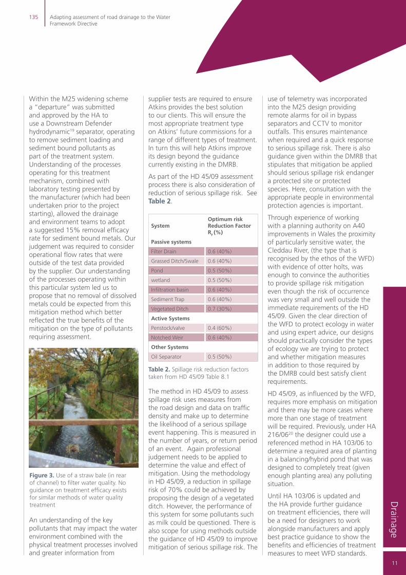
Without clear guidance on the efficacy of vegetative treatment systems one way of improving accuracy of assessment of the potential of treatment measures is through a written “departure” to the HA. Bespoke mitigation such as straw bales provided in agricultural areas (and shown in Figure 3) will provide levels of mitigation not addressed in HD 45/09. So far the approach of the Highways Agency via the DMRB has been to consider mitigation through vegetative treatment systems to some extent, but there is also the potential for proprietary systems to replicate natural drainage and provide treatment.
Table 1. Source Table 3.2 HA 103/06 that summarises water treatment information to be used in assessment of highway impact on the water environment
135 Adapting assessment of road drainage to the Water Framework Directive
11
Drainage
use of telemetry was incorporated into the M25 design providing remote alarms for oil in bypass separators and CCTV to monitor outfalls. This ensures maintenance when required and a quick response to serious spillage risk. There is also guidance given within the DMRB that stipulates that mitigation be applied should serious spillage risk endanger a protected site or protected species. Here, consultation with the appropriate people in environmental protection agencies is important.
Through experience of working with a planning authority on A40 improvements in Wales the proximity of particularly sensitive water, the Cleddau River, (the type that is recognised by the ethos of the WFD) with evidence of otter holts, was enough to convince the authorities to provide spillage risk mitigation even though the risk of occurrence was very small and well outside the immediate requirements of the HD 45/09. Given the clear direction of the WFD to protect ecology in water and using expert advice, our designs should practically consider the types of ecology we are trying to protect and whether mitigation measures in addition to those required by the DMRB could best satisfy client requirements.
HD 45/09, as influenced by the WFD, requires more emphasis on mitigation and there may be more cases where more than one stage of treatment will be required. Previously, under HA 216/0620 the designer could use a referenced method in HA 103/06 to determine a required area of planting in a balancing/hybrid pond that was designed to completely treat (given enough planting area) any polluting situation.
Until HA 103/06 is updated and the HA provide further guidance on treatment efficiencies, there will be a need for designers to work alongside manufacturers and apply best practice guidance to show the benefits and efficiencies of treatment measures to meet WFD standards.
supplier tests are required to ensure Atkins provides the best solution to our clients. This will ensure the most appropriate treatment type on Atkins’ future commissions for a range of different types of treatment. In turn this will help Atkins improve its design beyond the guidance currently existing in the DMRB.
As part of the HD 45/09 assessment process there is also consideration of reduction of serious spillage risk. See Table 2.
SystemOptimum risk Reduction Factor RF (%)
Passive systems
Filter Drain 0.6 (40%)
Grassed Ditch/Swale 0.6 (40%)
Pond 0.5 (50%)
wetland 0.5 (50%)
Infiltration basin 0.6 (40%)
Sediment Trap 0.6 (40%)
Vegetated Ditch 0.7 (30%)
Active Systems
Penstock/valve 0.4 (60%)
Notched Weir 0.6 (40%)
Other Systems
Oil Separator 0.5 (50%)
Within the M25 widening scheme a “departure” was submitted and approved by the HA to use a Downstream Defender hydrodynamic19 separator, operating to remove sediment loading and sediment bound pollutants as part of the treatment system. Understanding of the processes operating for this treatment mechanism, combined with laboratory testing presented by the manufacturer (which had been undertaken prior to the project starting), allowed the drainage and environment teams to adopt a suggested 15% removal efficacy rate for sediment bound metals. Our judgement was required to consider operational flow rates that were outside of the test data provided by the supplier. Our understanding of the processes operating within this particular system led us to propose that no removal of dissolved metals could be expected from this mitigation method which better reflected the true benefits of the mitigation on the type of pollutants requiring assessment.
Table 2. Spillage risk reduction factors taken from HD 45/09 Table 8.1
An understanding of the key pollutants that may impact the water environment combined with the physical treatment processes involved and greater information from
Figure 3. Use of a straw bale (in rear of channel) to filter water quality. No guidance on treatment efficacy exists for similar methods of water quality treatment
The method in HD 45/09 to assess spillage risk uses measures from the road design and data on traffic density and make up to determine the likelihood of a serious spillage event happening. This is measured in the number of years, or return period of an event. Again professional judgement needs to be applied to determine the value and effect of mitigation. Using the methodology in HD 45/09, a reduction in spillage risk of 70% could be achieved by proposing the design of a vegetated ditch. However, the performance of this system for some pollutants such as milk could be questioned. There is also scope for using methods outside the guidance of HD 45/09 to improve mitigation of serious spillage risk. The

12
Where vegetative treatment systems are considered in scheme design, in addition to guidance within the DMRB (HA103/06), there will also be a need to obtain and apply cross sector research information on mitigation efficacy rates and best practice for operation. The requirement for this information will be likely to increase with the greater requirements for use of SUDS following the FWMA, being applicable to both local authorities and the Highways Agency.
In addition to the planning for mitigation a method to respond to pollution incidents and to maintain pollution treatment features should be a standard provision with Atkins designed road schemes. At present there is no requirement within HD 45/09 to provide either a method for maintenance or a method for response to a pollution incident. However, within the design of the M25 drainage scheme the incorporation of alarms (within bypass separators), CCTV and a central management system for maintenance all added value to providing a quick response to pollution incidents should they occur.
An important consideration for effective application of treatment systems includes provision of adequate maintenance plans and consideration of maintenance within the design and consultation process. Historically drainage systems have suffered a lack of maintenance in some regions and resources to improve maintenance will continue to be stretched in the near future. Continued negotiation with the Environment Agency, Internal Drainage Boards, local authorities and other interested parties will ensure access to mitigation features will not hinder the effectiveness of treatment measures.
Summary
The application of the WFD through relevant guidance has required highway engineers and environmental teams to consider catchment wide, ecological effects of highway run-off including sediment discharge and compliance with a broader range of new water quality standards that reflect the current legal framework.
Although the current DMRB goes a long way to address the requirements of the WFD, there are still areas that can be improved in future iterations. A better understanding of the influence of sediments and the need to study the physical changes to watercourses along with effectiveness of mitigation are all areas that will need to be addressed in the near future.
In considering how to meet the standards, Atkins will be looking for opportunities to provide better treatment solutions for highways discharges which will allow new development to enhance our water environment rather than impact upon it. At present the existing driver for improvement of the water environment has been led by the Highways Agency, highways authorities, HD 45/09 and the Priority Outfall Assessment programme. However, where urban run-off from roads may be shown to be contributing to failure of WFD sample points, there may be a driver through River Basin Management Plans for further improvement of discharge from our road network.

135 Adapting assessment of road drainage to the Water Framework Directive
13
Drainage
References
1. Water Framework Directive 2000/60/EC.
2. HD 45/09 Road Drainage and the Water Environment DMRB, Volume 11 Section 3 Part 10.
3. BBC 31/12/2010 http://www.bbc.co.uk/news/uk-england-12098028.
4. Schedule 23 2.1 (3) b M25 contract.
5. Environment Agency WFD River Classification maps http://maps.environment-agency.gov.uk/wiyby/wiybyController?topic=wfd_rivers&layerGroups=default&lang=_e&ep=map&scale=3&x=456769.4583333337&y=302349.6249999998#x=527956&y=386044&lg=1,7,8,9,5,6,&scale=1.
6. Final RBMP http://www.environment-agency.gov.uk/research/planning/33106.aspx.
7. Memorandum of Understanding between the Environment Agency and the Highways Agency http://www.ha-partnernet.org.uk/portal/server.pt/community/memorandum_of_understanding/717.
8. The EC Freshwater Fish Directive (2006/44/EC).
9. Johnson, I and Crabtree RW, 2007, Effects of soluble pollutants on the Ecology of receiving waters, WRc Plc, Report No. UC 7486/1, UK Highways Agency.
10. DMRB Vol 11 Section 3 Part 10 3.14-3.16.
11. HADDMS http://www.haddms.co.uk/.
12. HA 103/06 Table 3.2 DMRB Volume 4 Section 2 Part1.
13. The Long term monitoring of pollution from Highway Run off: Final Report R&D technical report, P2-038/TR1 Moy, F, Crabtree RW and Simms, T.
14. The SUDS manual c697, CIRIA, 2007, London.
15. Sustainable Drainage Systems. Hydraulic, Structural and water quality advice, C609, London, 2004 CIRIA
16. The Flood and Water Management Act (c29) April 2010.
17. The SUDS manual c697, CIRIA, 2007, London.
18. The Flood and Water Management Act (c29) April 2010.
19. Downstream Defender http://mx1.hydro-intl.com/stormwater/downstream.php.
20. HA216/06 Road drainage and the water environment, 2006, DMRB superseded November 2009.

14

Drainage
136
15
John Wotherspoon
Group Engineer
Highways & Transportation
Atkins
IntroductionAtkins was appointed to work on the drainage designs for improvements to the Manchester Metrolink Phase 1 & 2 works and has been part of the Engineering Support Services Team for the GMPTE (now Transport for Greater Manchester – referred to as TfGM from here on). This commission was let to draw upon the drainage experience of the author, who had also worked on Nottingham Express Transit (NET Line 1) and was the principal drainage designer for the latest upgrade to the Blackpool & Fleetwood Tramway. These second generation tram systems had the same drainage problems to solve as their forerunners had overcome. Some of the tracks will be on former railway lines, so similar drainage techniques to Network Rail standards for ballasted track can be used and are not discussed further in this paper. Interesting drainage techniques to relearn relate to the urban realm, when groove rails are usually to be found, either on a segregated section of highway or in pedestrian areas, sometimes referred to as a trambahn, or on carriageways fully integrated with vehicular traffic, with the tram given priority at traffic lights and junctions. There are no new drainage techniques to be learned; only reapplication of those known to earlier drainage engineers.
Tram drainageAbstract
Trams have been in use in the UK for more than a century, 2010 being the 125th anniversary of Blackpool’s famous electric trams - one of the very first in the world and the first in the UK. Many other cities followed Blackpool’s example, but from the middle of the 20th century, most of these were closed down and the tracks ripped up for scrap or buried under tarmac. However, in April 1992, Greater Manchester’s Metrolink opened to passengers. The Bury and Altrincham lines were the first to open, followed by the Eccles line in July 2000. Many other cities in the UK now have, or are planning, tram systems, including Nottingham, Edinburgh, plus Dublin LUAS in the Republic of Ireland. This paper sets down the drainage requirements for this second generation of UK trams, based on the author’s experiences on a number of these tram systems.
Figure 1 shows an extract from an Edgar Allen catalogue c.1920, which clearly shows the two main elements of point drains and transverse drains.
Drain Box in position
Truck Drain BoxFigure 1.
Modern products of a similar style are being used and good practice is being developed on the second generation of UK tram systems and in the recent multi-million pound refurbishment and upgrade of the Blackpool Tramway. Some examples of drainage products used recently are shown below, at Fleetwood (Figure 2), Metrolink City Centre renewals (Figure 3) and Dublin LUAS (Figure 4).

16
outlet to cross drains under the track, similar to the pipework in the right hand image.
Little design advice is currently available as to what can be considered good practice. The most authoritative guidance is given by the Office of the Rail Regulator (ORR) document “Railway Safety Publication 2, Guidance on tramways, November 2006”. Clause 119 states, “Grooved rails should have suitable drainage provided at appropriate intervals and locations (e.g. areas of ponding, bottom of gradients), and when laid in the highway, connected to surface water drainage systems. The drains should be capable of being easily cleaned to allow removal of sand and other debris. The provision of drainage slots should not render the rail incapable of providing sufficient support or guidance for trams. Note: The effect of the presence of rail grooves on highway drainage may be significant”.
Thus the two aspects to be dealt with are spacing, what is “appropriate”, and maintenance, how should a feature be “easily cleaned”?
During 2009, as part of the Metrolink Phase 3 implementation, a review of these issues was undertaken by Atkins on behalf of GMPTE. The elements of good design that were thought to be important are summarised below, from the three points of view of a tramway drainage designer, the Asset Manager for GMPTE and for Stagecoach Metrolink, which has operated the tram service and maintained the network since July 2007.
At Fleetwood, the existing track was drained using the Edgar Allen products from the 1920s or earlier. A replacement product for the point drain was recommended by Atkins to the contractor and this was adopted and can be seen on the left of the three images above. The choice was based on two of the key elements developed as good practice, described in more detail below. In particular, this product allowed for a 150mm groove length and a vertical
Figure 2.
Figure 3.
Figure 4.
Elements considered ‘good practice’
The key points from a designer’s perspective are:
• Maximum spacing of groove drains 60m for roads flatter than 2%
• Exceptionally increase to 100m
• For roads steeper than 2%, review the above criteria and perhaps allow greater spacing
• Outlet orientation vertical leaving the drainage unit, with minimum diameter 75mm
• Point drainage units on shared running
• Point or transverse drainage units if segregated
• Slot at least 20mm wide by 150mm long
• Slot smooth edged and chamfered
• An appropriately sized silt trap (perhaps a road gully) should be sited at or downstream of the groove drains, to allow easy and regular maintenance
• Owners and operators should agree funding of adequate maintenance of drainage features.
These key lessons were reinforced by a tramway Asset Manager to emphasise:
• The the geometry of, and relations between, the various road and track surfaces need to be understood to define the requirement for transverse drainage as opposed to a point drain on its own
• Drainage is needed at the bottom of a “valley”
• Drainage is needed to protect any set of points at the bottom of a gradient
• Intermediate drainage is needed on a gradient to catch detritus and prevent a build up further downhill
• Careful specification of the

136 Tram drainage
17
Drainage
Figure 5.
Figure 6.
Figure 7.
It is clear that good practice is being developed, though guidelines are not definitive. Products are still being trialled and the effectiveness of these assessed. Manufacturers producing well used products include ACO, Hauraton, Riecken, Hanning & Kahl and Birco. An area currently being addressed by work in Fleetwood and Dublin relates to the better cutting of the slots within the grooved rail. Over the last 20 years, this was improved from small, poorly cut grooves (Figure 5); to longer slots drilled and cut, though still with unintended irregularities to catch debris (Figure 6); to a slot milled in the rail, producing an even slot with no irregularities (Figure 7).
Problems associated with tram drainage insufficiency are illustrated by two Case Studies, “The effects of poor drainage on a tramway” and “Difficulty of maintenance affecting the performance of tramway operation”. These illustrate how elements of the developing concepts of good practice in UK tramways were put in place to improve the future maintainability of the Manchester Metrolink system, using existing maintenance operations to bring about necessary changes.
Case Study 1 - The effects of poor drainage on a tramway
Introduction
A major interchange between bus, Park & Ride and Metrolink was constructed at Shudehill in 2002, just a 5 minute walk from the Arndale Centre and located next to The Printworks, a state of the art entertainment complex located in the heart of Manchester City Centre with a range of restaurants, bars and clubs alongside a cinema and gym. This valuable additional asset to GMPTE was a retrofit to the existing City Centre tram link joining Victoria and Piccadilly Main Line stations, which had opened ten years previously in 1992.
The problem
Three issues combined to make the trackslab beneath the rails subside. First, the track was level; secondly, a significant catchment of tram and highway drainage fell towards this flat area; and thirdly, the block paving between the platforms proved not robust enough to shed all this water to the drainage channels and prevent water percolating through to the trackslab formation. Plate 1-1 (Figure 8) shows severe degradation of the track and the surrounding surfaces. The trackslab had sunk in places, giving rise to uneven ride quality through the tramstop. This
four foot, shoulder, six foot and cess profiles to avoid ponding.
The key points from an operator/maintainer perspective are:
• Groove slot machined and large/wide enough to cope with the odd leaf or other detritus. Narrow short slots no good
• Good drainage in front of all facing points
• No boxes on curves – risk of rail fracture
• Drainage solution should have the necessary volume/capacity within the point or transverse drain such that anything greater than a shower does not cause it to back up or require it to be cleaned out every week because of sludge build up within. Ideally a good clean at start of autumn and again in the spring with perhaps attention during winter as required should be the frequency that should be aimed for
• Access to the drainage box is easy i.e. easy removal of the lid, and large enough such that it can be cleaned, ideally by mechanised means (gully sucker) to speed up the maintenance process
• One size/type does not fit all; the appropriate drainage solution must be put in place dependant on the location and the objective, be it groove or switch tip drainage, point or transverse drainage, segregated or non-segregated, trafficked or non- trafficked locations
• The ideal spacing depends on circumstances at each groove drain location.

18
failure had occurred in less than 8 years use of the new tramstop. The City Centre track had already been scheduled for entire renewal in 2009, so the opportunity was taken to investigate the problem thoroughly and propose a more robust solution.
Plates 1-2 (Figure 9) and 1-3 (Figure 10) show how cores were taken of the existing trackslab. These led to the conclusion that the trackslab had failed to the extent that this would require total replacement. In addition, surveys were made of the catchments contributing surface water to the tramstop area.
Drainage survey
This was a simple visual survey of the area, assessing the position of existing road gullies, falls on the highways and tramway towards the tramstop and consideration of the highway drainage as it would have been prior to construction of the tramway. It was determined that Shudehill itself, several hundred metres of tramway and the tramstop itself all contributed surface water runoff, which congregated on the flat track area between the platforms. The tram movements and water led to failure of the block paving and generated sand and silt at ground level that blocked the linear drainage channels at the foot of the platform walls. This led to more water being retained in the tramstop area and the cycle of degradation continued. A study of As Built records demonstrated that adequate outfalls had been provided for the tramstop drainage, connecting to public combined sewers, but highway drainage on Shudehill had not been installed upstream of the tramway. The tramway created a new pathway for the highway runoff, rather than the water continuing on to gullies downstream of the route of the tramway, which would have happened pre Metrolink.
Maintenance
Regular maintenance of the drainage systems at the tramstop was not considered a priority, leading to total failure of the linear drainage system. Highway drainage maintenance was effective, but only of gullies already installed.
Improvements
Drainage to the formation was installed, the complete trackslab was replaced and drainage of the grooved rail was introduced. The existing outfalls from the tramstop drainage were utilised, but additional chambers and rodding points were included on the formation drainage,
Figure 8. Plate 1-1: Shudehill tramstop in Manchester, showing distressed tracks and surfacing
Figure 9. Plate 1-2: Ground investigation set up

136 Tram drainage
19
Drainage
Figure 10. Plate 1-3: Recovery of cores Figure 12. Plate 1-5: … and at tramstop
Figure 11. Plate 1-4: Groove drainage upstream of Shudehill …
to allow better maintenance facilities for the future. As well as improving the foundations for the trackslab, the formation drains provided outfalls for other drainage features introduced at the tramstop. This included transverse drains as shown in plates 1-4 (Figure 11) and 1-5 (Figure 12), a replacement of the linear drainage
channels at the foot of the platform walls and rodding accesses. Though it would have been preferable to increase the size of the channels, this proved impossible due to other tramway infrastructure, namely communication and power ducting, being located immediately below the channels. Thus like for like
replacement took place. The final improvement, not driven by the drainage needs, was the change of finished surface between and around the new grooved rails, from conventionally laid block paving on a sand bed to exposed aggregate concrete. This choice, driven by experience of the failure of the surfacing at Shudehill and other locations also reduced substantially the likelihood of further drainage failures. The work was completed between April and November 2009, when the cross city tramway was closed for renewal, and it is anticipated that such a renewal will not be necessary again for perhaps another 20 years. It was also recommended that Manchester City Council should install additional gullies on Shudehill to catch more of the highway runoff before it reached the tramway.
Conclusions
Detailing of drainage features at initial design can have implications on the life of transport infrastructure. In the case of a tramway, it is well known that rails wear out, particularly when sharp radii are

20
necessary to negotiate an existing city street layout. A need to renew the rails after a seventeen year life was not considered by Metrolink as unreasonable, but for the trackslab to have needed replacement as well can be considered an avoidable expense. Drainage failures were not the whole cause of the problem, but were certainly a contributing factor. Drainage improvements were introduced throughout the City Centre as part of the latest track renewals at locations identified as problematic. Surface finishes also changed, to improve the Manchester streetscape. A combination of these features is shown in Plate 1-6 (Figure 13), on Mosley Street, outside the City Art Gallery. The general area is shown as Plate 1-7 (Figure 14).
Case Study 2 - Difficulty of maintenance affecting the performance of tramway operation
Introduction
Metrolink carries nearly 20 million passengers every year, on three lines from Altrincham, Bury and Eccles into Manchester city centre. The Bury and Altrincham lines opened in 1992 and the Eccles line in 2000, creating a network of 37 stops covering 37 km (23 miles), served by a fleet of 32 trams. By 2012 four new lines will nearly double the size of the tram network with 20 miles of new track and 27 new stops. The new lines will go to Oldham and Rochdale, Chorlton, Droylsden and Media City. At Media City, an existing track crossover on the Eccles line needs to be brought into continuous use to allow the trams to access the new stop.
The problem
Though drainage of the grooved rail had been introduced for the Eccles extension of Metrolink, the
Figure 13. Plate 1-6: Groove drainage at Mosley Street
Figure 14. Plate 1-7: …by the City Art Gallery
drainage feature used could not be readily maintained. This allowed water from the road to the north of the Broadway tramstop to flow down the rail grooves. Water that falls on the four foot (between the rails) and the six foot (between the tracks) flows along the groove until the groove is full before it overflows to the roadway surface and flows to the kerbline to be collected by the highway drains. So, a relatively
light shower of rain produces a significant flow of water in the grooves, which flows through the tramstop, collecting grit all the time, then discharges close to the points mechanism which forms the crossover. The build up of grit and debris makes the operation of the points unreliable.
Plates 2-1 (Figure 15) to 2-4 (Figure 16) illustrate the elements of the

136 Tram drainage
21
Drainage
Figure 15. Plate 2-1: New Media City extension
Figure 19. Plate 2-5: A light summer storm
Figure 16. Plate 2-2: Broadway stop, no groove drainage
Figure 20. Plate 2-6: The effect!Figure 18. Plate 2-3: The crossover
Figure 17. Plate 2-4: The points mechanism
Figure 21. Plate 2-7: Groove drainage upstream of Broadway
Figure 22. Plate 2-8: … extending for a kilometre
problem; the new track to Media City under construction; the existing Broadway tramstop, some 200m long with no groove drainage; the crossover to be brought into constant service; and the points mechanism adjacent to the grooved rail end. A light summer storm of about fifteen minutes duration filled the groove and brought silt down to the points mechanism. The build up of debris can be seen adjacent to the rail. This is illustrated above in Plates 2-5 (Figure 19) & 2-6 (Figure 20).
Maintenance
The road leading to Broadway tramstop (South Langworthy Road) has a wide six foot (the space between the two tram tracks) marked as a ghost island with pedestrian refuges. It is a busy urban road, as can be seen in Plates 2-7 (Figure 21) and 2-8 (Figure 22). The groove rail point drains can be seen within the four foot (the space between the two rails of a single tram track). The tops of these are secured by two Allen screws and there is a 50mm horizontal outlet.
To clean these, traffic management would be needed to run traffic on the six foot. This can only be achieved during a night time closure of the lane. On a site inspection to review the problem described, it was observed that most of the slots and the boxes below appeared to be silted up, which suggested that maintenance is problematic. This is clearly not an easily maintained feature.
Asset management
GMPTE has appointed an asset manager to assist the processes as necessary. Day to day operation and maintenance are the responsibility of the Operating Company, at the time of writing Stagecoach Metrolink. The maintainer used its term contractor to inspect one of these features in detail. First the sewer was surveyed and a 150mm connection was located, this being constructed as part of the sewer diversion works for the tram. Then, using an endoscope it was shown that the track drainage box has a 50mm corrugated pipe on

22
its outlet. This pipe is approx 400mm in length and then connects into the 150mm plastic drainage pipe which then runs into the 525mm main sewer. The box lifted was on the cess rail (nearer the kerbline) and thus it can reasonably be assumed that the 150mm pipe spans the four foot.
Improvements
An improvement to the drainage was proposed. The style of groove drain box used for the Metrolink Eccles extension is no longer favoured, with an irregular cut in the groove and only a 50mm horizontal outlet for water and silt. A point drain product, shown in Plate 2-10 (Figure 24), had recently been installed in Fleetwood, as part of the Blackpool and Fleetwood Tramway Improvements, with a well machined slot and a 100mm vertical outlet. It was recommended that one or more of the existing groove drains on South Langworthy Road should be changed for a more easily maintained feature. Other improvements recommended were for a variety of transverse track crossings by several manufacturers, to give the opportunity to trial products, regularly used in Europe, for the first time in the UK.
Within the tramstop area and in other areas of segregated tramways running on grooved rails, it is more usual to use a transverse drain. Two manufacturers’ products were recommended for trial at the Broadway tramstop. One of these is heavy duty and is claimed by the manufacturer as suitable for use in shared carriageway as well as on segregated areas. This manufacturer also offers a lighter duty ‘hinged’ product that is more easily opened. Examples of these are shown in Plates 2-11 (Figure 25) & 2-12 (Figure 26), both of which have vertical 100mm outlets through the trackslab to a bend and outfall pipe below. An alternative, with a horizontal pipe beneath the track, was also considered for trial (Plates 2-13 (Figure 27) & 2-14 (Figure 28)).
Figure 23. Plate 2-9: Groove drainage upstream of Broadway
Figure 27. Plate 2-13: Transverse drain
Figure 24. Plate 2-10: … and at Fleetwood
Figure 25. Plate 2-11: Transverse drain in a trafficked area
Figure 28. Plate 2-14: … details of undertrack drain
Figure 26. Plate 2-12: … and a segregated track
These recommendations were left with TfGM, who would have to determine an appropriate procurement strategy for the works and assess the timing so that the works would complement the first of the new Metrolink Phase 3 extensions opened, to Media City in September 2010. TfGM determined that it would be impractical to replace any of the defective point drains on South Langworthy Road, but two transverse installations were completed, a narrower one at the inbound end and a wider one at the outbound end of the Broadway tramstop area. These were both supplied by the first of the two manufacturers suggested by Atkins.

136 Tram drainage
23
Drainage
Figure 29. Plate 2-15: Wide transverse drain Outbound …
Figure 31. Plate 2-17: The points able to function well
Figure 32. with clean trackbed downstream of drains
Figure 30. Plate 2-16: … and narrow Inbound
These were photographed in August 2012 after they had been operating for twelve months and were observed to be successful. The tram service to Media City service operates as a shuttle during the daytime; every other tram terminating at Media City, the others travelling to Eccles, but in the evenings and at weekends all trams run via Media City. Thus, the formerly unreliable points are now operating on a daily basis and are no longer a maintenance issue. The completed installations are illustrated below in Plates 2-15 to 2-18 (Figures 29-32). Atkins offered the client an understanding of the nature of the problem, a range of options to provide a solution and support for TfGM to procure this based on knowledge of the various manufacturers’ products and contact details for pricing and supply.
Stakeholder engagement
Tramways are being delivered using Design & Build forms of contract. Extensions or improvements to existing systems in the UK and the complete creation of a new system have been commonplace for the last 20 years. The owners of the assets created will generally be a local authority or a Passenger Transport Executive. This body will have a long term responsibility for maintenance, such as the 125 years that Blackpool Borough Council and its preceding bodies have been successfully running a tram system in Blackpool and Fleetwood. The operator may change, perhaps as further extensions are added. TfGM is working with its third operator since it opened in 1992. Designers for the drainage of trams can work for any of the above stakeholders. The parameters for the design cannot be too prescriptive and each stakeholder can have a slightly different emphasis on the outcome of the design. All parties need to engage in these issues from preliminary design through to construction.
Conclusions
From this case study, specific to tram drainage but of interest to all drainage construction, the elements of the need for designing with maintenance in mind are well illustrated. It is not easy to predict how the future needs of a transport system will change. In this case, an operational feature (the crossover) will change from occasional to hourly use. The cost of failure of the asset (the points) will be on the operational efficiency of the tram system. Inbound trams would be unable to call at the highly prestigious Media City tramstop. As this will be the heart of the BBC, the ensuing poor publicity could, literally, be broadcast far and wide! Thus the failure of a simple drainage feature, or the poor choice of a product for reasons of economy, expedience or availability, has far reaching conclusions.

24
Acknowledgements
Thanks to my colleague, Chris Potter, for providing his constructive review of the script. Constructive comments from Matthew Hack, the Asset Manager for Transport for Greater Manchester (TfGM) on a draft of this paper are gratefully acknowledged, as is the permission of TfGM to publish the two case studies. These were initially prepared as part of the CIRIA RP941 draft report published in 2012 “Transport infrastructure drainage: condition appraisal and remedial treatment” and CIRIA’s inspiration for this paper is recognised.

Environment &
Sustainability137
25
Tom Singleton
Vice President
Water & Environment
Atkins North America
Pam Latham
Principal Technical Professional
Water & Environment
Atkins North America
IntroductionThe Winter Haven City Commission approved the Sustainable Water Resource Management Plan in 2010, establishing a new direction for managing water resources in Winter Haven and the Peace Creek Watershed (Atkins 20102). The Sustainability Plan outlines an approach for managing watershed resources that relies on existing natural infrastructure, thereby reducing costs to the public and providing multiple benefits with respect to water quality, water supply, flood protection, and natural systems.
Impervious urban land uses and conversion of wetlands to developed land uses degrade watershed
Winter Haven Chain of Lakes: conservation and restoration targets for sustainable and innovative watershed planningAbstract
A model for identifying conservation and restoration targets in the Peace Creek watershed was developed in response to the Sustainable Water Resource Management Plan completed for the City of Winter Haven, Florida (Singleton 20111) and is presented here. A GIS button tool was developed to automate scenarios of various combinations and rankings of water resource functions (e.g. surface and ground water) and subsequently identify conservation and restoration targets in the watershed. These targets provide a mechanism for selecting locations for conceptual design projects and feasibility studies, identifying opportunities for trade-offs between development and resource benefits, quantifying loss of ecosystem services, and mitigating for that loss. The resource targets provide a context to guide land use ordinances, development regulations, and develop incentives for protecting water resources.
Identifying areas for future restoration and conservation is critical to planning efforts in the Peace Creek watershed. Conservation and restoration targets are based on available watershed-level data so that potential projects may be ranked relative to each other and displayed as maps. Once targets become part of the planning process, specific projects can be selected based on site-specific feasibility criteria and development can be directed consistent with the restoration and conservation targets.
Animated and pdf versions of the Plan can be obtained at: http://northamerica.atkinsglobal.com/WHSP
functions, which in turn contribute to flooding, soil erosion, water (and water supply) pollution, and loss of recreational uses of waters. Integrating ecosystem benefits or services into land use planning has only recently become part of a sustainable planning approach (Collins et al. 20073). The Development of Conservation and Restoration Targets for Sustainable Water Resource Management (or Resource Targets) further develops the concepts presented in the Sustainable Water Resource Management Plan by presenting a model for identifying conservation and restoration target areas for the watershed.

26
• A GIS button was developed that allowed the user to evaluate changes in resource functions in various combinations (e.g. with and without habitat data)
• Data were integrated to provide composite water resource data layers
• Locally-specific data were added to the watershed-scale data to refine areas for which more specific data were available.
Ninety-six available data sources were reviewed for data relevant to resource functions and benefits. Available data that were insufficient in areal extent to cover the watershed, characterized by limited or no relationship to evaluating the resource benefit, or unquantifiable, were excluded from further analyses. Fifteen individual data layers were subsequently retained to characterize the resource function layers.
Data were first evaluated for relevance to particular resource function, such as surface water, groundwater, or habitat (surface and groundwater were further segregated into surface water quality
recharge is a water resource function and a measureable attribute (i.e. recharge potential), that translates to resource benefits, including water supply, water quality, fish and wildlife habitat, etc. The approach relied on four primary components (outlined below).
• Conservation and restoration targets were developed at a scale consistent with that of available, relevant data. For example, land cover data are available for the entire watershed and illustrate differences between the more developed northern and less developed southern watershed
• Data were acquired for these analyses and, in later steps, were ranked as a means of evaluating the landscape, both temporally (historic vs. existing) and spatially (across the watershed). This precludes the use of data that are not available for the entire watershed
• Data were ranked as a means of scoring and comparing data that have different units of measure
The purpose of the project was to develop conservation and restoration targets that can be used to support future land use decisions in the City of Winter Haven and surrounding Peace Creek watershed. To accomplish this, available data were screened for relevance and scale appropriateness and a Geographic Information System (GIS) platform was used to create GIS layers that represent five water resource functions: surface water quantity, surface water quality, groundwater quantity, groundwater quality, and habitat. Data intercepts representing the links between resource functions (e.g. surface water quantity) and benefits (e.g. water supply) were used to develop the resource function layers (Figure 1). Analysis of pre-developed (or un-impacted) conditions of resources provided the basis for target areas: those with the least (or no) difference with respect to undeveloped (e.g. circa 1940s) conditions are referred to here as conservation targets, while areas that exhibit greater changes are referred to as restoration targets.
The product is a map of water resource management “target areas”, represented by water resource data layers, in the watershed. In addition to spatial extent of targets, this study documented an estimated loss of 20,815 acre-feet of surface water storage loss since the 1940s as a result of the loss of wetlands and reduced lake levels.
Methods
Five resource functions were defined to characterize the hydrologic and ecological character of the Peace Creek watershed: groundwater quantity, groundwater quality, surface water quantity, surface water quality, and habitat. A resource benefits matrix (Table 1) summarizes the links between the resource functions (GIS layers) and resource benefits. For example, groundwater
Figure 1. Example of integration of data layers used to evaluate resources and develop resource conservation and restoration targets

137 Winter Haven Chain of Lakes: conservation and restoration targets for sustainable and innovative watershed planning
27
Environment &
Sustainability
Table 1. Resource benefit function matrix: indicates relationships between resource functions and benefits (x indicates relationship)
*Data layers included under a previous resource function. FLUCFCS = Florida Land Use Cover and Forms Classification System, used in combination with other resource function data layers as a measure of urbanization impacts. NA=not
Water Resource Functions
Data Attribute (defined below table)
Water Resource Benefits (Targets)
Water Supply
Water Quality
Flood Protection
Fish and Wildlife
Recreation/ Cultural Resources
Groundwater
StoragePotentiometric surface
x x x
Discharge (to surface water)
NA x x x x
Recharge Recharge x x x x
Hydraulic conductivity
Soils x x x
Quality RCRA, SWAA
Surface Water
Nutrient transport/mediation
Impairment x x
Sediment stabilization
NA x x x
StorageWater levels (natural wetlands
x x x x x
Discharge (to surface and ground water)
Recharge* x x x x x
Water transport Connectivity* x x x x
Quality Impairment
Habitat
Climate regulation
NA x x
Nutrient assimilation
NA x x x
Groundwater mediation
Groundwater* x x x x
Surface water mediation
Surface water* x x x
Soil formation Soils* x x x x
Connectivity SHCA x x x x x
Effect on other resource functions**
FLUCFCS x x x x x
and quantity and groundwater quality and quantity). Some data were then combined with a second data layer to produce the appropriate data field for analysis. For example, land use was used in combination with recharge data to identify high vs. low recharge areas. Integrated (or composite) data layers for a resource function were developed from the individual data layers by summing and averaging data for each location across the watershed, thereby integrating GIS data layers into a composite resource function (e.g. surface water quality) data layer. The composite layer is the equivalent of the resource function layer (Figure 1). For example, the habitat function is a composite of listed species data, habitat type, land use, and adjacent land use, and also addresses connectivity among habitats that typically reflect streams and wetlands. The process of data compilation, evaluation integration into GIS, and ranking and evaluation throughout the watershed is summarized in Figure 2. The more detailed data and ranking process are outlined in Table 2.
In the same way that non-parametric statistics rely on ranked data when conventional parametric analyses are inappropriate, data were ranked as a means of allowing comparisons across resources with different characteristics and units of measure. Altered conditions were assigned a value = “-5” (representing restoration), while relatively pristine conditions were assigned a value = “+5” (representing conservation) with respect to a particular resource function (e.g. surface water storage). Values of “0” were assigned to data if a restoration or conservation condition could not be established. Therefore, areas in which the potentiometric surface has declined were ranked “-5” while areas where it has not declined were ranked “+5”. Similarly, undeveloped high and moderate infiltration soils would be considered conservation potential, while developed high and moderate
infiltration soils were identified for restoration.
Final composite water resource data layers and the water resource management target areas were based on scenarios in which various resource function layers were assigned different priorities (e.g. 1
for surface water quantity and 2 for groundwater quantity). A location for which averaged ranks among the five resource function layers indicated relatively pristine water quality conditions, unaltered groundwater and surface water conditions, and “natural” fish and wildlife habitat also represented a location with

28
a high conservation potential. In contrast, a location in which all these resources are altered would be assigned a high value for potential restoration.
Although the process described here was carried out for all five water resource functions, a single example (surface water quantity) is presented to illustrate the development of a potential water resource target.
Surface water quantity
The surface water quantity resource function represents the change in surface water storage between historic (1940s) and current conditions. Restoration is a measure of lost water storage, but not the overall quality of, for example, a
Figure 2. General approach to developing conceptual conservation and restoration resource targets
wetland that still has storage but has been impacted by agricultural practices for decades. Therefore, this resource function represents potentially recoverable water storage in the case of restoration targets and opportunities for water storage management in the case of conservation targets. Connectivity is difficult to measure, but is important when considering the historic surface water connections. While connectivity is not measured for surface water, it can be superimposed on the targets map to examine its influence. Connectivity is a measure of habitat, however, and is typically consistent with surface water connections.
The areal extent of the surface water quantity data layer includes
historical and current wetlands and lakes, including wetlands associated with water conveyances such as streams and creeks, floodplain wetlands, isolated wetlands, and National Wetlands Inventory (NWI) wetlands (which include seasonally inundated wetlands). Federal Emergency Management Agency (FEMA) floodplains are designated for flood risk and insurance purposes (based on the one percent annual flood occurrence or “100-year floodplain”) and are not, therefore, included in the analysis. In the Peace Creek watershed, however, historic wetlands closely follow the FEMA 100 year floodplain.
Data layers used to develop the surface water quantity resource function layer are listed and

137 Winter Haven Chain of Lakes: conservation and restoration targets for sustainable and innovative watershed planning
29
Environment &
Sustainability
1. P
RO
MPT
: Ch
oo
se d
ata
laye
rs f
or
each
wat
er r
eso
urc
e fu
nct
ion
Data LayersResource Function
2. P
RO
MPT
: Ch
oo
se d
ata
laye
r to
co
mb
ine
Data Additions/Combinations
3. P
RO
MPT
: Ch
oo
se d
ata
fiel
d t
o b
e u
sed
fo
r ra
nki
ng
fo
r ea
ch d
ata
set
Data Fields
4. P
RO
MPT
: Ran
k p
aram
eter
s in
ch
ose
n d
ata
fiel
d
Rank Value
5. P
RO
MPT
: Wei
gh
Res
ou
rce
fun
ctio
n la
yer
Pro
du
ct: C
on
serv
atio
n/
Res
tora
tio
n T
arg
et S
cen
ario
2009
Lan
d U
se
2008
Po
ten
tio
met
ric
Surf
ace
Wat
ersh
ed
Del
inea
tio
n
-5 0 5
Floridan recharge
Groundwater Quantity
x RechargeDeveloped/ Recharge > 10
Undeveloped/ Recharge 1 to 10
Undeveloped/Recharge > 10
Pre-development potentiometric surface
x Change Change = 0 NA Change <> 0
Soils x InfiltrationDeveloped/ A, B
C, D, B/DUndeveloped/ A, B
Source Water Assessment Areas (SWA)
Groundwater Quality
500-ft BufferInside 500-ft buffer
Outside 500-ft buffer
NA
Resource Conservation and Recovery Act Facilities
Groundwater Quality
500-ft BufferInside 500-ft buffer
Outside 500-ft buffer
NA
Historical land use (wetlands) Surface Water
Quantity
x PRE_FLUCFCSLoss of Storage
Gain /No Change in Storage
2009 land use FLUCFCSCODE
Ridge/valley lakes
Surface Water Quantity
x x ImpactedDeveloped/Impacted
Insufficient data
Undeveloped/ Not Impacted
Significant surface water
Priority NA 0 Priority 1 - 7
Water quality status
x Impaired ImpairedInsufficient data
Not Impaired
Strategic Habitat Conservation Areas (SHCA)
Habitat
Priority NA NA Priority 1 - 5
Historical land use
PRE_FLUCFCS NA NACypress, Sand Pine
2009 land use FLUCFCSCODEResidential, Tree Crops
NACypress, Pine Flatwoods
Table 2. Data layer compilation, ranking, and mapping for conservation and restoration targets development (left to right)
Table 3. Data representing surface water quantity resource functions
Table 4. Ranking scale used to assign priority for the surface water quantity resource function
described in Table 3 and rankings are listed in Table 4. The process of data selection, ranking, and application is summarized in Table 5. For example, the change in surface water storage was calculated from a comparison of hydrologic conditions (hydroperiods - see below) under historic and current land use/land use using GIS and follows the approach used for the Natural Systems Model the South Florida Water Management District uses to model pre-drainage conditions in the Everglades (SFWMD 20104) and refined as presented for the Collier County Watershed Management Plan (Atkins 20105).
Data Layer Description Source, Date
Historic Land Use Historic land use against which to measure changes in land use
Atkins, as developed for Peace River Cumulative Impacts Study
Current Land UseCurrent land use for comparison with historic land use
SWFWMD 20096
Hydrology
Depth and duration of natural communities to evaluate changes in surface water storage between current and historic land use.
Duever et al. 19867
Attribute Used in Ranking Rank
Change in surface water storage
Loss/gain in hydroperiod -5
No change in hydroperiod 5

30
Hydrology scoring is the functional value of a land parcel based on the persistence of historical hydrologic reference conditions. Hydroperiods are estimated based on the typical range of depth (inches) and duration (days) of inundation of the vegetation community. No change from historic conditions would result in a score of “+5”, while total loss of hydrology (e.g. a cell dominated by a historic condition wetland or open water body but which now experiences no inundation) would result in a score of “-5”. The hydrology score was applied on a 750 feet x 750 feet cell basis.
The hydrology score for a cell/parcel is based on the ratio of the existing depth and duration in comparison to the historic condition, adjusted to a scale of “-5” to “+5”. For instance, a site that historically had an average hydroperiod of six months and an average inundation of 12 inches, but which currently is inundated for only two months at an average depth of four inches (i.e. the site currently experiences one-third of the depth and duration of the historic condition for that site), would have a hydrology score of “-1.67”. More simply, a cypress swamp that was converted to an urban land use would be represented by a loss of storage and have a rank of “-5”, while a cypress swamp that retained its hydrology would have a rank of “+5”.
Surface water quantity restoration and conservation targets are mapped in Figure 3 (the footprint of a locally proposed road, the Central Polk Parkway, is displayed in maps throughout this document as for reference). The most conspicuous feature is the pattern of ridge lakes (along the Winter Haven Ridge) designated as predominantly restoration (brown) lakes and the “valley” lakes (on the adjacent, lower, Polk Upland) designated as predominantly conservation (green) lakes. This is consistent with the result of previous studies of the Winter Haven Lakes that point to
Current Land Use/ Land Cover
Historic Wetland and Lakes Land Cover
Land Cover Class
Cypress Swamp
Freshwater Marsh
Mesic Hammock
Swamp Forest
Lakes Total
Agriculture -90 -91 0 -344 -101 -626
Cypress 0 0 0 -39 -2 -41
Freshwater Marsh
555 0 0 -936 -4,156 -4,537
Golf Course -60 -37 0 -258 -62 -417
Mesic Flatwood -136 -128 0 -108 -20 -392
Mesic Hammock
-331 -37 0 -517 -77 -962
Pasture & Bare Ground
-2,742 -1,189 0 -5,811 -319 -10,061
Swamp Forest 936 39 0 0 -187 788
Urban -618 -421 0 -1,915 -1,460 -4,414
Lakes 859 839 0 930 0 2,628
Wet Prairie -497 -291 0 -1,782 -211 -2,781
Total -2,124 -1,315 0 -10,780 -6,596 -20,815
Table 5. Calculated changes in surface water storage from historic to current land use/land cover conditions (acre-feet)
the groundwater dependence of the ridge lakes and the changes in these lakes as a consequence of the declining aquifer. The valley lakes have a greater surface water influence, which is also reflected in the more elongate shapes compared with the round ridge lakes.
The shift from native uplands to urban development represents a change in surface water storage in the watershed, although the urban areas actually had greater storage. Consequently, urban areas that were formerly native uplands were assigned a value of “0” to avoid the appearance that “restoration” was recommended solely based on a gain in surface water storage. In addition to mapping the changes in surface water from historic to current conditions, the loss of storage represented by the changes was calculated. For example, a conversion from wetlands such as cypress swamp and wet prairie to agriculture and urban land uses represents a particular loss of surface water storage that may be restored, although restoration of agricultural lands is more likely than restoration of urban lands.
A total of 2,124 acre-feet (Table 4) of historic water storage in cypress swamp has been lost due to conversion to many different land uses (e.g. 90 acre-feet of storage to agriculture, 60 acre-feet to golf course, 618 acre-feet to urban development). Similarly, 6,596 acre-feet of former lake/open water storage have been converted to other land covers/uses (e.g. 101 acre-feet of historic lakes converted to agriculture). Overall, this indicates an estimated 20,815 acre-feet of surface water storage have been lost, primarily due to a conversion of wetlands and lakes to developed (urban, agriculture, and golf courses) land uses (Table 5). These losses were due primarily to loss in forested wetlands (cypress swamp and swamp forest, 12,904 acre-feet) and open water/lakes (6,596 acre-feet).
In terms of restoration opportunities, some of the conversions may represent opportunities to regain water storage. For example, a total of 10,061 acre-feet of former wetlands and open water were lost due to conversions to pasture and bare ground (Table 5) and represent a loss of the same amount of storage

137 Winter Haven Chain of Lakes: conservation and restoration targets for sustainable and innovative watershed planning
31
Environment &
Sustainability
Figure 3. Composite surface water quantity resource function layer
that may be seen as a restoration opportunity.
Numerous lakes are mapped as restoration (brown) due to storage loss, while some are mapped as conservation (green) due to gains. Losses and gains are based on comparisons between historic and existing land use cover (i.e. areal extent of lakes) and typical changes in depth associated with changes in land use. For example, a loss of 10 acres of a lake due to a change from open water to urban would be a greater loss than a shift to a marsh or forested wetland because
of the differences in water depths. Although changes in lake levels have not been evaluated for many lakes, a previous study (Atkins 2009) documented an average decline of 5 feet in lake levels in the Winter Haven Chain of Lakes. Although data are available that estimate 1850s land cover using 1927 soils maps, the soils maps are not pre-development and differences between the 1927 and 1940s land cover maps appear negligible. Consequently, the existing historic (circa 1940s) and current (2009) data are considered the best data available for this project.
Conservation and restoration resource target scenarios
The five individual resource function layers (groundwater quality, groundwater quantity, surface water quality, surface water quantity, and habitat) were merged to generate a conservation and restoration resource target map that identifies areas for restoration or conservation, based on a comparison of historic and existing conditions (e.g. historic and existing water storage) or the presence/absence of historical attributes (e.g. permeable land surface). The five resource layers were, metaphorically speaking, “stacked” together, and the data in each of the five layers were averaged together for each pixel location across all five resource layers (refer back to Figure 2) to produce a single map. Conservation and restoration resource targets have been developed at a scale appropriate to the available data. Because the land use regulatory system operates at different political and legal scales than the natural scales of ecosystems (Arnold 20078), however, individual projects developed as part of future efforts will have to be examined at the appropriate scale.
The GIS button tool was developed to automate scenario development of the resource target map (outlined previously in Figure 1). Using the tool, different scenarios are developed by assigning different weights to resource function layers (Figure 4). A scenario would be based on the relative importance of each resource function layer and the footprint of the proposed project and the current or future land use, i.e. the user could examine the total impact of a proposed project on the five resource layers combined and/or one or more layers at a time. If the surface water quality and quantity functions were considered adequate for a particular purpose,

32
such as evaluating potential National Pollutant Discharge Elimination System (NPDES) permitting, the other layers could be omitted. One example is presented here.
An alternate scenario, Scenario 1, can be generated if more importance to the surface water quantity resource function layer is preferred when compared to the other resource function layers. Assigning the surface water quantity layer a weight of “3” results in a scenario in which surface water quantity has three times more influence than the other four resource function layers (Figure 5). Similar to Scenario 1, the restoration targets are predominantly in the heavily developed City of Winter Haven. However, weighting the surface water quantity resource function more than the other resource layers results in a shift to include many more of the green conservation areas (e.g. in the northern portion of the watershed).
Composite water resource data layers and resource targets
Combining resource function layers into composite data maps provides a means of identifying areas with restoration and conservation potential with respect to more than one layer. Surface water and
groundwater quantity resource function layers had the most comprehensive data of the five resource function layers and are of particular interest at both state and local levels. To further focus on restoration and conservation targets with higher priority, the 30th percentile for groundwater target areas and 100 percent of the potential surface water storage were retained for displaying water resource data layers and targets. In addition, “noise” was removed from the final map by omitting contiguous
Figure 4. Scenario 1: example of GIS button tool for surface water quantity weight=“3” and remaining resource function layers are assigned weight = ”1”
Figure 5. Scenario 2: conservation and restoration resource target map when surface water quantity weight = “3” and remaining resource function layers have weights =”1”
areas greater than 20 acres in size (100 percent of the target areas are retained in the project GIS layers to ensure data integrity). The color scheme was changed to include the two different resource layers in this case (blue for surface water and green for groundwater). These two data layers were combined and are mapped in Figure 6 and illustrate the concentration of groundwater targets in the northern portion of the watershed and surface water targets in the southern portion of the watershed.

137 Winter Haven Chain of Lakes: conservation and restoration targets for sustainable and innovative watershed planning
33
Environment &
Sustainability
Figure 6. Composite water resource data layers for the Peace Creek Watershed

34
In some cases, discrepancies were noted in the water resource data map/model due to false historic wetland signatures. In one case, land use/land cover data classify a lake (Lake Lulu) as restoration and conservation. The conservation designation is a result of the persistence of the wetland forest despite lower water levels, i.e., the wetland tree species are long-lived and will persist for years and the area therefore exhibits no change from historic to current. Similarly, a piece of property identified as wet prairie because of a “wet” signature is in pasture, but the wetland signature remains and the property is designated as potential conservation. To address these issues, project-specific data/studies can be used to make cosmetic revisions without altering the raw data.
Conclusions: water resource targets
Conservation and resource targets provide a mechanism for the City of Winter Haven to select locations for conceptual projects and feasibility studies, identify opportunities for trade-offs between development and ecosystem benefits, quantify a loss of services, and mitigate for that loss. For example, opportunities to mitigate for impacts to groundwater elsewhere in the watershed can be readily identified. The resource targets provide a context for land use measures to guide revisions to land use ordinances and development regulations and to develop incentives for protecting water resources.
Identification of areas for future restoration and conservation is even more important from a planning perspective. The resource targets developed for the Peace Creek watershed provide locations for restoration and conservation in the watershed, based on available watershed-level data. Once these targets become part of the planning process, specific restoration and
conservation projects can be located appropriately throughout the watershed, while development can be directed in a way that is consistent with the restoration and conservation targets.
Local governments face challenges to using land use planning to protect water resources and associated community benefits. Therefore, to the extent that restoration and conservation of priority locations cannot be accomplished through land planning and other non-structural controls, engineering and other structural controls will need to be identified. These controls are less effective and more costly to implement than non-structural controls and, therefore, local governments should consider leveraging its land planning authorities, including using incentives to protect water resources, to the greatest extent possible. The City of Winter Haven may choose to implement monitoring and other feedback mechanisms for adaptive management of water resources. Identifying the resource targets allows the implementation of strategies to examine specific projects, options for land use planning, and private sector concepts such as mitigation banking and regional stormwater ponds. Some communities have established goals that target tree canopy increases in recognition of air and water benefits, while others have imposed regulatory jurisdiction over land use to prevent development because the costs associated with land use regulation and land acquisition were less than the costs of building additional water treatment facilities that would be necessary if the development was permitted.
The City of Winter Haven may, as another example, choose to restore a portion of an estimated 20,815 acres of surface water storage lost to conversions to other land uses (primarily urban and agriculture). Or, stakeholders may choose to
focus restoration efforts on only restorable (non-urban) areas, or any combination of these efforts. Estimates of loss of water storage were consistent with previous patterns identified for water quantity and reflect differences in ridge (Winter Haven Ridge) and valley (Polk Uplands) geology that dominate the watershed. Water storage restoration targets included predominantly the ridge lakes in the Southern Chain of Lakes, while lakes identified for conservation included mostly valley lakes in the Northern and Interior Chain of Lakes (consistent with results of the recently completed study of the Interior Chain of Lakes). Another practical option is restoration of storage that can be recovered without impacting adjacent land owners. In contrast, areas of water storage that remain unchanged (or with little change) are identified as conservation targets and include Lakes Hamilton, Henry, Haines, Rochelle, and Smart in the Northern Chain of Lakes.
The resource targets developed for this project provide a model for revising the City’s ordinances and developing incentives to protect water resources in the watershed. These mechanisms will be developed as part of the next step in carrying out the Sustainability Plan. This report presents the resource targets that can be used to evaluate, direct, and support land use decisions that contribute to sustainability in the entire watershed, including the portion of the watershed that forms the Sapphire Necklace, which was the focus of the Sustainability Plan. The resource targets are presented as conservation and restoration maps that provide the watershed context in which to focus and develop a range of water management alternatives. These alternatives, as well as the rules, ordinances, and other planning mechanisms to implement them, will be accomplished as part of future planning and design charrettes with City staff.

137 Winter Haven Chain of Lakes: conservation and restoration targets for sustainable and innovative watershed planning
35
Environment &
Sustainability
Acknowledgements
The Atkins project team included Tom Singleton, Pam Latham, Ph.D., Katherine Anamisis, Emily Keenan, and Leslie Gowdish, Ph.D. Special acknowledgement to Mike Britt, P.E., Director, Natural Resources Division, City of Winter Haven, who conceived of the original sustainability plan. Also, thanks to Jackie Cooper, Atkins, who provided valuable editing assistance.
References
1. Singleton, T.J. 2011. Sustainable Water Resource Management Plan. Atkins Technical Journal 6, paper 92: 99-109.
2. Atkins. 2009. Sustainable Water Resource Management: A Conceptual Plan for the Peace Creek Watershed and the City of Winter Haven, Florida. Final Report to the City of Winter Haven.
3. Collins, S.L., S.R.Carpenter, S.M/ Swinton, D.E. Orenstein, D.L. Childers, T.L. Gragson, N.B. Grimm, J.M. Grove, S.L Harlan, J.P. Kaye, A.K. Knapp, G.P. Kofinas, J.J. Magnuson, W.H. McDowell, J.M Melack, L.A. Ogden, G.P. Robertson, M.D. Smith, and A.C. Whitmer. 2010. An integrated conceptual framework for long-term social–ecological research. Ecological Society of America: Frontiers in Ecology and the Environment. DOI:10.1890/100068.
4. SFWMD. 2011. Natural System Model. http://www.sfwmd.gov/portal/page/portal/xweb%20-%20release%202/natural%20system%20model.
5. Atkins. 2010. Collier County Watershed Management Plan. Final Report to Collier County.
6. SWFWMD (Southwest Florida Water Management District). 2009. Land use data. Available from website. http://www.swfwmd.state.fl.us/data/gis/layer_library/?search=fluccs.
7. Duever, J.J., J.E. Carlson, J.F. Meeder, L.C. Duever, L.H. Gunderson, L.A. Riopelle, T.R. Alexander, R.L. Myers, and D.P. Spangler. 1986. The Big cypress National Preserve, National Audobon society Research Report No. 8. New York. 455 p.
8. Arnold, C.A. 2007. The Structure of the Land Use Regulatory System in the United States. Journal of Land Use and Environmental Law 22(2): 441.

36

Environment &
Sustainability138
37
Francisco J. Pérez Aguiló
Senior Scientist/ Project Manager
IntroductionApproximately 9,860 tons of municipal solid wastes (MSW) are generated in Puerto Rico (the Island, see Figure 1) every day (ADSPR, 2003). Approximately 15.3% of this mass is presently segregated for recycling (ADSPR, 2008). The remaining 8,351 tons per day (tpd) is disposed-off in landfills. During the 100 or so years since we became a throw-away society (Life, 1955; as cited in Rathje & Murphy, 2001), the MSW stream in Puerto Rico has resulted in approximately 2,000 acres (8,093,745 square meters) of opened or closed landfills (ADSPR, 2003), for an average rate of twenty new acres (404,687 m2) of landfill per year. Seven out the nineteen (36.8%) sites listed as the most polluted in Puerto Rico by the USEPA (2011) are former landfills. See Figure 2 for the location of the 31 landfills still in operation in 2007.
Landfills vs. incinerators: identification and comparison of the hazards posed by the toxic emissions associated with the disposal of municipal solid waste in Puerto Rico
Abstract
Hazardous Air Pollutants (HAPs) emitted by landfills and incinerators were estimated and compared. The USEPA quantified one Puerto Rico (PR) landfill’s emissions using LandGEM Version 3.02, and those results were extrapolated for PR’s land-filled municipal solid waste (MSW) stream. The USEPA Emission Factors (1995) were utilized to estimate HAP emissions from the incineration of this MSW. Results are that PR landfills emitted 106.2 tons per year (tpy) of 26 HAPs during 2008: All are Volatile Organic Compounds, eight are known carcinogens (11.4 tpy) and seven are possible or potential carcinogens (17.1 tpy). Incinerators would emit 394.2 tpy of eight HAPs: 98.8% would be hydrochloric acid (389.5 tpy), five known carcinogens (0.6 tpy) and one is a potential carcinogen (0.1 tpy). HAPs were also estimated using data from five operating incinerators (range: 39.4 - 1,245.8 tpy, average: 493.3 tpy), the worst performer would emit fewer known/possible/potential carcinogens (13.3 tpy) than landfills do (28.5 tpy).
Figure 1. Location map

38
the biochemical reactions that occur within landfills, and they are emitted to the atmosphere in the landfill gas stream (Elias-Castells, 2005). Table 1 shows the typical landfill contaminants. These gasses range in impact from nuisance odors to toxicity (USEPA, 1999; Chian & DeWalle, 1979).
3. The liquids deposited in the landfill will find their way to the
MSW has been deposited in the landfill, and its generation continues for decades or even hundreds of years (E.A., 1997; ATSDR, 2001; Ferry, 2002; USEPA, 1998c, 2002 and 2005a; Durmusoglu, Yavuz & Tuncay, 2005).
2. Volatile and semi-volatile gases can be present in the MSW stream deposited in landfills. These are also formed during
Figure 3 illustrates two Island landfills.
Landfills and incinerators pose hazards to public health and the environment, but which one poses fewer hazards? This study investigates the toxic emissions for existing, modern incinerators, and compares them with the toxic emissions presently emitted from landfills in the Island.
Sanitary landfills
The sanitary landfill is the most widely utilized disposal method for solid wastes (UNEP, 2002) and is the least expensive alternative when land is not in short supply. Landfills generate no visible emissions, except during fire events, and require very little manpower and equipment. However, MSW buried in a landfill remains there for hundreds or thousands of years (Rathje & Murphy, 2001). The following are notable exceptions:
1. Methane (CH4) and Carbon Dioxide (CO2) will result from the biological decomposition of the organic matter, according to the following formula: Organic substances + microbial activity = heat + CH4 + CO2 + contaminants This “landfill gas” will invisibly ventilate out of crevices, the landfill surface, or a system designed for this purpose (Elías-Castells, 2005). CH4 and CO2 are important greenhouse gasses; however, CO2 is removed from the atmosphere by photosynthetic organisms (algae and plants), whereas CH4 is not, and is a greenhouse gas 21 times more potent than CO2 (USEPA, 1998c and 2005b). The methane fraction of this “landfill gas” is sometimes used as fuel (USEPA; 1998b, 2002). Landfill gas generation peaks approximately 30 years after
Figure 2. Location of Puerto Rico Landfills
Figure 3. Examples of Puerto Rico Landfills
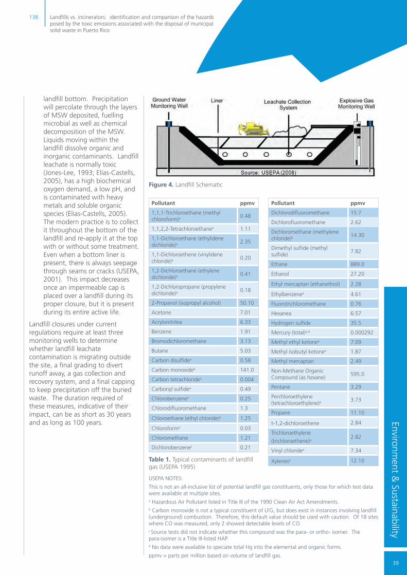
138 Landfills vs. incinerators: identification and comparison of the hazards posed by the toxic emissions associated with the disposal of municipal solid waste in Puerto Rico
39
Environment &
Sustainability
Table 1. Typical contaminants of landfill gas (USEPA 1995)
USEPA NOTES:
This is not an all-inclusive list of potential landfill gas constituents, only those for which test data were available at multiple sites.a Hazardous Air Pollutant listed in Title III of the 1990 Clean Air Act Amendments.b Carbon monoxide is not a typical constituent of LFG, but does exist in instances involving landfill (underground) combustion. Therefore, this default value should be used with caution. Of 18 sites where CO was measured, only 2 showed detectable levels of CO.c Source tests did not indicate whether this compound was the para- or ortho- isomer. The para-isomer is a Title III-listed HAP.d No data were available to speciate total Hg into the elemental and organic forms.
ppmv = parts per million based on volume of landfill gas.
landfill bottom. Precipitation will percolate through the layers of MSW deposited, fuelling microbial as well as chemical decomposition of the MSW. Liquids moving within the landfill dissolve organic and inorganic contaminants. Landfill leachate is normally toxic (Jones-Lee, 1993; Elías-Castells, 2005), has a high biochemical oxygen demand, a low pH, and is contaminated with heavy metals and soluble organic species (Elias-Castells, 2005). The modern practice is to collect it throughout the bottom of the landfill and re-apply it at the top with or without some treatment. Even when a bottom liner is present, there is always seepage through seams or cracks (USEPA, 2001). This impact decreases once an impermeable cap is placed over a landfill during its proper closure, but it is present during its entire active life.
Landfill closures under current regulations require at least three monitoring wells to determine whether landfill leachate contamination is migrating outside the site, a final grading to divert runoff away, a gas collection and recovery system, and a final capping to keep precipitation off the buried waste. The duration required of these measures, indicative of their impact, can be as short as 30 years and as long as 100 years.
Figure 4. Landfill Schematic
Pollutant ppmv
1,1,1-Trichloroethane (methyl chloroform)a
0.48
1,1,2,2-Tetrachloroethanea 1.11
1,1-Dichloroethane (ethylidene dichloride)a
2.35
1,1-Dichloroethene (vinylidene chloride)a
0.20
1,2-Dichloroethane (ethylene dichloride)a
0.41
1,2-Dichloropropane (propylene dichloride)a
0.18
2-Propanol (isopropyl alcohol) 50.10
Acetone 7.01
Acrylonitrilea 6.33
Benzene 1.91
Bromodichloromethane 3.13
Butane 5.03
Carbon disulfidea 0.58
Carbon monoxideb 141.0
Carbon tetrachloridea 0.004
Carbonyl sulfidea 0.49
Chlorobenzenea 0.25
Chlorodifluoromethane 1.3
Chloroethane (ethyl chloride)a 1.25
Chloroforma 0.03
Chloromethane 1.21
Dichlorobenzenec 0.21
Pollutant ppmv
Dichlorodifluoromethane 15.7
Dichlorofluoromethane 2.62
Dichloromethane (methylene chloride)a
14.30
Dimethyl sulfide (methyl sulfide)
7.82
Ethane 889.0
Ethanol 27.20
Ethyl mercaptan (ethanethiol) 2.28
Ethylbenzenea 4.61
Fluorotrichloromethane 0.76
Hexanea 6.57
Hydrogen sulfide 35.5
Mercury (total)a,d 0.000292
Methyl ethyl ketonea 7.09
Methyl isobutyl ketonea 1.87
Methyl mercaptan 2.49
Non-Methane Organic Compound (as hexane)
595.0
Pentane 3.29
Perchloroethylene (tetrachloroethylene)a
3.73
Propane 11.10
t-1,2-dichloroethene 2.84
Trichloroethylene
(trichloroethene)a 2.82
Vinyl chloridea 7.34
Xylenesa 12.10

40
Incinerators as alternative
The controlled burning of MSW was developed to reduce the volume of MSW to be disposed, convert the caloric output into energy, and recover materials that survive the process:
Organic substances + O2 = heat + CO2 + H2O + contaminants
The USEPA (1995) has compiled a list of typical emissions that come out of the smokestack for the various types of incinerators under different scenarios of emissions control, see Table 2.
The more efficient the combustion process, fewer contaminants are generated (Elias-Castells, 2005). However, heavy metals and the un-combusted organic substances that remain in the ash residues, including those formed during incomplete combustion can make incinerator ash disposal a problem (USEPA, 1998a). These “incinerator solid wastes” occupy a small fraction of the volume of the original MSW, reducing the required landfill capacity needs by 85% (Renova, 2000). Significantly reducing the volume of the material to be disposed in landfills significantly reduces the disposal problem.
Just like the decomposers in the biosphere, incinerators return energy and materials for anthropogenic (human) consumption (Husar, 1994): Energy (approximate rate of 0.029 megawatts per ton of MSW), steam, construction aggregate (91.6 kg/ton of MSW), ferrous (38.1 kg/ton of MSW) and non-ferrous (3.6 kg/ton) metals (Renova, 2000), as illustrated in Figure 5?
Modern incinerator technologies include the processing of the fly-ash to trap the contaminants it contains and make them unavailable to the environment. For instance, incinerator ash containing 7.5% lead and 0.2% cadmium, encapsulated in a sulphur polymer with additives
Table 2. Typical Emissions for incinerators with and without emissions control
Pollutant
Emissions Control Technology
Uncontrolled Emissions (kg/Mg)
Spray Drier/ Fabric Filter Emissions (kg/Mg)
Arsenicb 0.00214 0.0000212
Cadmiumb 0.00545 0.0000136
CDD/CDFc 0.000000835 0.0000000331
CO2 985 *
COd 0.232 *
Cromiumb 0.00449 0.0000150
HClb 3.20 0.106
Mercuryb 0.0028 0.0011
Nickelb 0.00393 0.0000258
NOxd 1.83 *
Leadb 0.107 0.000131
Particulate Matera 12.6 0.0311
SO2 1.73 0.277
USEPA NOTES:
CO2 emitted from incinerators may not increase total atmospheric CO2 because emissions may be offset by the uptake of CO2 by regrowing biomass.
Emission factors should be used for estimating long-term, not short-term emission levels. This particularly applies to pollutants measured with a continuous emission monitoring system (e.g., SO2).
kg/Mg = kg of emissions per Megagram (1,000,000 grams or 1.0 metric tons) of solid waste combusted.
* = Same as “uncontrolled” for these pollutants.a PM = Filterable particulate matter, as measured with EPA Reference Method 5.b Hazardous air pollutants listed in the Clean Air Act.c CDD/CDF = total tetra- through octa-chlorinated dibenzo-p-dioxin/chlorinated dibenzofurans. 2,3,7,8-tetrachlorodibenzo-p-dioxin, and dibenzofurans are hazardous air pollutants listed in 1990 Clean Air Act.d Control of NOx and CO is not tied to traditional acid gas/PM control devices.e Calculated assuming a dry carbon content of 26.8% for feed refuse.
results in leachable levels below allowable concentrations (USEPA, 1996). The technology to turn ash residues into stable cement-like substances (Keck and Seitz, 2002; Buckley and Pflughoeft-Hassett, 2006) has found many constructive applications (NYT, 1919, USDOE, 2000; USDOT, 2000). At a minimum, these stabilization technologies allow the solid residue to be disposed in landfills with minimal potential for generation of toxic leachate and occupying a small fraction of the landfill space when compared with the original MSW.
Not in my backyard
A basic comparison between these technologies indicates that the incinerators fare much better than landfills in the following categories: Emission of greenhouse gasses (Solano et al., 2002; USEPA, 2006a), discharge of toxic leachate (Jones-Lee, 1993; USEPA, 1996; USDOE, 2000; USDOT, 2000; Keck and Seitz, 2002; Buckley and Pflughoeft-Hassett, 2006), duration of the impact (Elias-Castells, 2005), materials recovered (landfills have none), power generation (USEPA, 2006a), jobs creation (USDOT, 2000;

138 Landfills vs. incinerators: identification and comparison of the hazards posed by the toxic emissions associated with the disposal of municipal solid waste in Puerto Rico
41
Environment &
Sustainability
RWB, 2001; CEPA, 2003) and land consumption (Renova, 2000). Public perception, however, is an area where incinerators fare far worse than landfills, even though landfills also suffer from the not in my back yard (NIMBY) syndrome (ANL, 1994; McCarthy, 2004).
The most consistent argument in opposition to the incinerators is their toxic emissions (McCarthy, 2004). Earlier versions of the incinerator sparked this reputation: Incomplete combustion, inappropriate or non-existent emissions controls, and other factors yielded large quantities of toxic contaminants in their atmospheric emissions (NYT, 1919; USEPA, 1995 and 1998a). Many of the reports attacking incinerator emissions refer to the Harrisburg, Pennsylvania Incinerator, which began operations in 1972 (USEPA, 1985) and emitted at least two orders of magnitude more dioxins than the average U.S. incinerator of its time (USEPA, 1997a). Others refer to the Columbus, Ohio Incinerator, which operated between 1983 and 1994, during which time it emitted a full one third of the dioxin emissions in the U.S. (Lorber et al., 1998).
Do modern incinerators contaminate as much? And, how do their emissions compare
The Experiment
The Arecibo landfill was used as a sample of the Hazardous Air Pollutants (HAP) emissions generated from the disposal of MSW in Puerto Rico landfills. It serves the sixth largest municipality in the Island and receives its fourth largest waste stream. A study by the ADSPR (2003) reported the weight in tons per year (tpy) and volume of MSW disposed in all 31 Island landfills for one week each during 2003, and the waste composition at 12 selected landfills and two transfer stations. Some stations, including the Arecibo landfill, were re-sampled to measure
Figure 5. Incinerator schematic for a 910 tpd facility
Figure 6. Example of a 2,700 tpd incinerator
the impact of the holiday MSW stream and other fluctuations.
The HAPs, those listed in Subchapter I, Part A, § 7412 of the U.S. Clean Air Act, were quantified for the hypothetical emissions of MSW management in Puerto Rico using incinerators. HAP emissions data (waste processed and emissions) from five incinerators were also obtained from existing United States facilities through available U.S. Environmental Protection Agency (EPA) databases. The emissions data obtained from these incinerators were scaled for 8,301 tpd, in accordance with the following equation:
Emissions from all Puerto Rico MSW incinerated = Results for incinerator Y X 8,301 tpd tpd MSW incinerator Y
Landfill HAP emissions data are not so readily available. Until recently (USEPA, 1997b) there was no requirement for landfill gas monitoring. Even the 1997 regulation, which imposed gas monitoring to active landfills, was limited to the largest 5% of landfills (greater than 2.5 million metric ton capacity). Therefore, existing data needed to compare toxic releases from landfills are limited. However,
1000ton
MSWEntersProcess
TippingFloor
99% to Shredders
PRF toBoilers 95%
Ferrous
MetalRecovery
Boiler
75MW of Electricity
Fly Ash
Bottom Ash 12%
7.7% to Landfill
86% Sold
14% used in-house
0.7% Bulky and hazardous objects
Ferrous Metals 2.0%
Boiler AggregateTM 9.8%
Non-Ferrous 0.4%
Ferrous 2.1%
OverallTo Energy: 76.6%Recovered: 13.7%Landfilled: 9.6%

42
QCH4 KL0e-ktij
Mi
10=
n 1
t=1 j=0.1∑ ∑
the USEPA has compiled a list of Emission Factors, which consist of averages of the available data of acceptable quality, obtained from hundreds of actual test results performed on actual emission sources, and are representative of long-term averages for each type of facility (USEPA, 1995 and 2008).
This study utilized the USEPA’s Landfill Gas Emissions Model (LandGEM, Version 3.02) (USEPA, 2005a), prepared for the Arecibo Landfill by the USEPA Region 2. The data collected by the USEPA (2009) in support of their emissions model of the Arecibo Landfill covered a total of 33 years, from 1973, the year it opened, through 2006. The LandGEM estimates emission rates for all landfill gases, including: methane, carbon dioxide, non-methane organic compounds, and individual air pollutants, and is based on the following first-order decomposition rate equation to quantify emissions from the decomposition of MSW in landfills:
Where:
QCH4 = annual methane generation in the year of the calculation (m3/year)
i = 1 year time increment
n = (year of the calculation) - (initial year of waste acceptance)
j = 0.1 year time increment
k = methane generation rate (year-1)
Lo = potential methane generation capacity in cubic meters per mega-gram (m3/Mg) of MSW.
Mi = mass of waste accepted in the ith year in Mg
tij = age of the ith section of waste mass Mi accepted in the ith year (decimal years, e.g., 3.2 years)
The results obtained for the Arecibo Landfill, which accepts an average of 541 tpd, or 6.5% of the 8,301
tpd deposited in Puerto Rico landfills daily, were extrapolated by this study for the entire Island through the following equation:
Emissions Estimate for all MSW deposited in Puerto Rico landfills = LandGEM Results, Arecibo Landfill X 8,301 tpd 541 tpd
The results from the previous exercise, namely the landfill gas emissions estimate, were used to estimate the toxic contaminants emitted to the atmosphere from landfills in Puerto Rico using the Emission Factors compiled by the USEPA (1995). In the case of landfill emissions, these are expressed as a ratio of a pollutant emitted per volume of landfill gas (i.e. mg/m3).
To estimate emissions of non-methane organic contaminants from landfills, the following equation is used by LandGEM:
QP = 1.82 QCH4 + Cp ÷ (1x10⁶)
where:
QP = Emission rate of pollutant P, m3/yr
QCH4 = CH4 generation rate, m3/yr, from LandGEM results (above)
CP = Concentration of P in landfill gas (Emission Factor, ppmv)
1.82 = Multiplication factor, assumes that approximately 55% of landfill gas is CH4 and 45% is CO2, N2, and other constituents
The Emission Factors (USEPA, 1995) for MWCs were used to estimate the Island’s emissions if all MSW land-filled in Puerto Rico were processed with incinerators.
Mass of toxics as a surrogate for risk
The mass of HAPs emitted should be a strong indication of the overall risk that landfills and incinerators pose. Mass is the most important factor in risk assessment for one
simple reason: The amount of a toxic substance is always the numerator in the risk factors, such as dose (mg/Kg or milligrams of contaminant per kilogram of body mass) or exposure (mg/m3, milligrams of contaminant per air volume). Take away the mass of the contaminant and the risk goes to zero. Increase the mass of a contaminant available for exposure and the risk increases accordingly.
Results: landfill emissions in Puerto Rico
There are 46 non-methane organic contaminants in landfill gas, of which 26 belong to the HAP category. A total of 106.2 tpy of HAPS were emitted at ground level from open and closed landfills throughout the Island in 2008, including 248,686 tpy of carbon dioxide and 90,637 tpy of methane, for a total of 2,152,063 tpy of greenhouse gas CO2-equivalents; (USEPA, 2005b). Table 3 shows the resulting emissions for the sample and for the Island.
Of the 26 HAPs in Puerto Rico landfill gas, seven are known carcinogens (Vinyl Chloride with 5.2 tpy, Acrylonitrile with 3.8 tpy, Benzene with 1.7 tpy, Ethylene Dichloride with 0.5 tpy, Propylene Dichloride with 0.2 tpy, Chloroform with 0.04 tpy, Carbon tetrachloride with 0.007 tpy, and Ethylene dibromide with 0.002 tpy) and a further seven are possible carcinogens or potential occupational carcinogens (Tetrachloroethylene with 6.9 tpy, Trichloroethylene with 4.2 tpy, Ethylidene Dichloride with 2.7 tpy, 1,1,2,2-Tetrachloroethane with 2.1 tpy, Methyl chloride with 0.7 tpy, 1,4-Dichlorobenzene(p) with 0.3 tpy, and Vinylidene Chloride with 0.2 tpy), for a total of 11.4 tpy of known carcinogenic HAP emissions and 17.1 tpy of potentially or possible occupational carcinogenic HAP emission.
With the exception of a minute amount (0.001 tpy) of mercury, most of the 106.15 tpy of HAPs

138 Landfills vs. incinerators: identification and comparison of the hazards posed by the toxic emissions associated with the disposal of municipal solid waste in Puerto Rico
43
Environment &
Sustainability
CAS Number Chemical NameArecibo Landfill
Puerto Rico
74-82-8 Methane 6,430 90,637
124-38-9 Carbon Dioxide 17,643 248,686
79-34-5 1,1,2,2-Tetrachloroethane 0.1 2.1
106-46-7 1,4-Dichlorobenzene(p) 0.02 0.3
107-13-1 Acrylonitrile 0.3 3.8
71-43-2 Benzene 0.1 1.7
75-15-0 Carbon disulfide 0.04 0.5
56-23-5 Carbon tetrachloride 0.0005 0.007
463-58-1 Carbonyl sulfide 0.02 0.3
108-90-7 Chlorobenzene 0.02 0.3
67-66-3 Chloroform 0.003 0.04
100-41-4 Ethyl benzene 0.4 5.5
75-00-3 Ethyl chloride (Chloroethane) 0.07 0.9
106-93-4 Ethylene dibromide (Dibromoethane) 0.0002 0.002
107-06-2 Ethylene dichloride (1,2-Dichloroethane) 0.03 0.5
75-34-3 Ethylidene dichloride 0.2 2.7
110-54-3 Hexane 0.5 6.4
7439-97-6 Mercury Compounds 0.00005 0.0007
74-87-3 Methyl chloride (Chloromethane) 0.05 0.7
71-55-6 Methyl chloroform 0.05 0.7
78-93-3 Methyl ethyl ketone (2-Butanone) 0.4 5.8
108-10-1 Methyl isobutyl ketone (Hexone) 0.2 2.2
78-87-5 Propylene dichloride 0.02 0.2
127-18-4 Tetrachloroethylene (Perchloroethylene) 0.5 6.9
108-88-3 Toluene 2.9 40.6
79-01-6 Trichloroethylene 0.3 4.2
75-01-4 Vinyl chloride 0.4 5.2
75-35-4 Vinylidene chloride 0.02 0.2
1330-20-7 Xylenes (isomers and mixture) 1.0 14.4
Total HAP emissions: 7.5 106.2
Table 3. Landfill gas and hazardous air pollutant (HAP) estimates for the Arecibo Landfill and for Puerto Rico based upon the 2008 MSW deposit rate
All emissions figures in tons per year (tpy). Significant digits were removed for clarity.
Figure 7. Comparison (in tpy) of HAP emissions in Puerto Rico: Landfills v. incinerators
in landfill gas consist of volatile organic compounds (VOCs), some halogenated, with a heavier-than-air vapour (mean vapour density = 3.8, range = 1.7 – 6.5). Their high density keeps these contaminants close to the ground, available to human receptors and the food chain. VOCs also participate of the atmospheric photochemical reactions and contribute significantly to the formation of ground-level ozone and smog (Elias-Castells, 2005).
Results: incinerator emissions
Should the five incinerators sampled process all of the Island’s MSW, they would generate anywhere from 39.4 to 1,245.8 tpy of HAPs, with an average of 493.3 tpy, see Figure 7.
The single largest HAP present in the emissions of the five incinerators evaluated is hydrochloric acid, which contributed anywhere from 99.0% to 99.8% of the HAP mass, with an average of 99.3%. Lead is the next most important component of the incinerator HAP emissions, comprising an average of 0.038%, with mass ranging from 0.04 to 13.07 tpy (average = 2.73). Mercury compounds followed in order of concentration, comprising an average of 0.054% of the emissions for all five incinerators. Mercury emission estimates using the various incinerators as models would range from 0.009 to 1.1 (average = 0.3) tpy. Cadmium is the fourth most important component of the HAP emissions, comprising an average of 0.011%, with a mass ranging from 0.00 to 0.24 (average = 0.06) tpy.
Another estimate of HAP emissions from incinerators was obtained from the USEPA’s Emissions Factors (USEPA, 1995 and 2003), which provide five technology scenarios: No emissions controls, electrostatic precipitators, spray dryer/electrostatic precipitator, duct sorbent injection/fabric filter, and spray dryer/fabric

44
MWC-A MWC-B MWC-C MWC-D MWC-EEmission Factors
tpy Received 2008 100,375 602,250 281,780 220,825 102,930 for MSW w/Spray Drier/Fabric Filter
MWC - PR MSW 2.7% 16.4% 7.7% 6.0% 2.8%
Emissions Multiplier 36.61 6.10 13.04 16.64 35.70
MWC PR MWC PR MWC PR MWC PR MWC PR
Hydrochloric acid 20.6 754.1 41.6 253.8 3.0 39.1 74.0 1,231.4 4.6 `64.6 389.5
Lead Compounds 0.001 0.04 0.03 0.2 0.02 0.3 0.8 13.1 0.003 0.1 0.5
Hexachlorobenzene 0.2 7.4
Mercury Compounds 0.005 0.2 0.05 0.3 0.001 0.01 0.07 1.1 0.0003 0.009 4.0
Cadmium Compounds 0.001 0.03 0.002 0.01 0.0008 0.01 0.01 0.2 0.05
Manganese Compounds 0.004 0.1
Polycylic Organic Matter 0.003 0.1
Formaldehyde 0.0002 0.007
Arsenio Compounds 0.0000002 0.000006 0.0009 0.005 0.08
1,3-Butadiene 0.00002 0.0007
Benzene 0.000020 0.0007
Beryllium Compounds 0.00006 0.0004
Dioxins & Furans 0.0000002 0.000006 0.000004 0.0001 0.0001
Naphthalene 0.000002 0.00008
Nickel Compounds 0.0000004 0.00002 0.09
Chromium Compounds 0.00000001 0.0000004 0.06
Total 20.8 761.9 41.7 254.3 3.0 39.4 74.9 1,245.8 4.6 164.9 394.3
Table 4. HAP Emissions from Incinerators: Sampled Incinerators, and USEPA’s Emission factors. Extrapolated for all MSW Landfilled in Puerto rico in 2008
All Emissions and MSW figures in tons peryear. Emission factors in kilograms per megagram of MSW. Estimates based upon the estimated 3,674,611 tpy MSW land-filled in the island (see Table 1). Decimal places rediced to the first non-zero to illustrate order of magnitude. Calculations with all significant figures. MSW= Municipal Solid Waste, MWC = Municipal Waste Combustor or incinerator, PR = Puerto Rico
filter. Each set of emissions control technologies has its strengths and its weaknesses (Elias-Castells, 2005), and may be installed in series for additional removal of contaminants.
The spray dryer/fabric filter technology was selected mainly due to the simplicity and effectiveness of this process: Water or partially treated wastewater (for re-use) is sprayed into the emissions, often with additives such as lime (CaCO3) or caustic soda (NaOH) for pH adjustment and contaminant adsorption. The spray lowers the emissions temperature to below the temperature of formation for dioxins and other organic pollutants (Lorber et. al., 1998; USEPA, 1997a, 1998a, and 2006b). As water evaporates to steam, the solids that are left behind
are trapped, forming a “cake” in the surface of the fabric filters, which further provides filtering and adsorption (Elias-Castells, 2005; and USEPA, 1998a, b, 2008). Spray dryer/fabric filter is also the most frequently used emissions control technology for incinerators in the United States (USEPA, 2003).
Total HAP emissions estimate using the Emissions Factors was 394.3 tpy. The single largest HAP present in the emissions, based on this national average is, again, hydrochloric acid. It comprised 98.8% of the HAP mass (389.5 tpy), followed by Mercury with 4.0 tpy (1.03%), Lead with 0.5 tpy (0.038%), Nickel with 0.09 tpy (0.024%), Arsenic with 0.08 tpy (0.020%), Chromium with 0.06 tpy (0.014%), Cadmium with
0.05 tpy (0.013%), and dioxins & furans with 0.0001 tpy (0.00003%). These are the only HAPs listed in the Emissions Factors (USEPA, 1995) for incinerators.
Out of the eight HAPs that would be emitted by incinerators, five are known carcinogens (Lead with 0.5 tpy, Arsenic with 0.08 tpy, Chromium with 0.06 tpy, Cadmium with 0.005 tpy, and Dioxins & Furans with 0.0001tpy) and one is a potential occupational carcinogen (Nickel with 0.09 tpy), for a total of 0.6 tpy of known carcinogen emissions and 0.09 tpy of potentially carcinogenic emission.
Incinerator emissions are discharged through a smokestack designed to the height necessary to ensure that emissions do not result in excessive
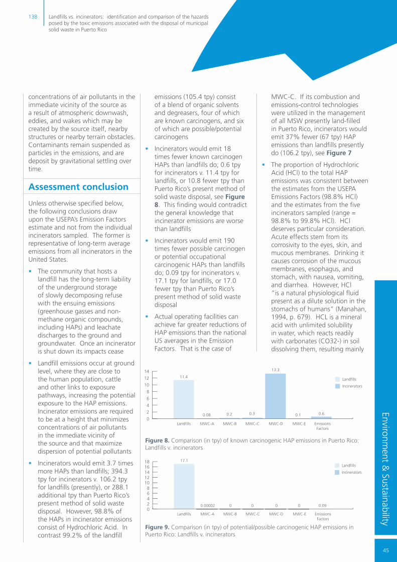
138 Landfills vs. incinerators: identification and comparison of the hazards posed by the toxic emissions associated with the disposal of municipal solid waste in Puerto Rico
45
Environment &
Sustainability
Figure 8. Comparison (in tpy) of known carcinogenic HAP emissions in Puerto Rico: Landfills v. incinerators
Figure 9. Comparison (in tpy) of potential/possible carcinogenic HAP emissions in Puerto Rico: Landfills v. incinerators
concentrations of air pollutants in the immediate vicinity of the source as a result of atmospheric downwash, eddies, and wakes which may be created by the source itself, nearby structures or nearby terrain obstacles. Contaminants remain suspended as particles in the emissions, and are deposit by gravitational settling over time.
Assessment conclusion
Unless otherwise specified below, the following conclusions draw upon the USEPA’s Emission Factors estimate and not from the individual incinerators sampled. The former is representative of long-term average emissions from all incinerators in the United States.
• The community that hosts a landfill has the long-term liability of the underground storage of slowly decomposing refuse with the ensuing emissions (greenhouse gasses and non-methane organic compounds, including HAPs) and leachate discharges to the ground and groundwater. Once an incinerator is shut down its impacts cease
• Landfill emissions occur at ground level, where they are close to the human population, cattle and other links to exposure pathways, increasing the potential exposure to the HAP emissions. Incinerator emissions are required to be at a height that minimizes concentrations of air pollutants in the immediate vicinity of the source and that maximize dispersion of potential pollutants
• Incinerators would emit 3.7 times more HAPs than landfills; 394.3 tpy for incinerators v. 106.2 tpy for landfills (presently), or 288.1 additional tpy than Puerto Rico’s present method of solid waste disposal. However, 98.8% of the HAPs in incinerator emissions consist of Hydrochloric Acid. In contrast 99.2% of the landfill
emissions (105.4 tpy) consist of a blend of organic solvents and degreasers, four of which are known carcinogens, and six of which are possible/potential carcinogens
• Incinerators would emit 18 times fewer known carcinogen HAPs than landfills do; 0.6 tpy for incinerators v. 11.4 tpy for landfills, or 10.8 fewer tpy than Puerto Rico’s present method of solid waste disposal, see Figure 8. This finding would contradict the general knowledge that incinerator emissions are worse than landfills
• Incinerators would emit 190 times fewer possible carcinogen or potential occupational carcinogenic HAPs than landfills do; 0.09 tpy for incinerators v. 17.1 tpy for landfills, or 17.0 fewer tpy than Puerto Rico’s present method of solid waste disposal
• Actual operating facilities can achieve far greater reductions of HAP emissions than the national US averages in the Emission Factors. That is the case of
MWC-C. If its combustion and emissions-control technologies were utilized in the management of all MSW presently land-filled in Puerto Rico, incinerators would emit 37% fewer (67 tpy) HAP emissions than landfills presently do (106.2 tpy), see Figure 7
• The proportion of Hydrochloric Acid (HCl) to the total HAP emissions was consistent between the estimates from the USEPA Emissions Factors (98.8% HCl) and the estimates from the five incinerators sampled (range = 98.8% to 99.8% HCl). HCl deserves particular consideration. Acute effects stem from its corrosivity to the eyes, skin, and mucous membranes. Drinking it causes corrosion of the mucous membranes, esophagus, and stomach, with nausea, vomiting, and diarrhea. However, HCl “is a natural physiological fluid present as a dilute solution in the stomachs of humans” (Manahan, 1994, p. 679). HCL is a mineral acid with unlimited solubility in water, which reacts readily with carbonates (CO32-) in soil dissolving them, resulting mainly

46
in calcium chloride (CaCl2), potassium chloride (KCl) or sodium chloride (NaCl); carbon dioxide and water, in accordance with the following equations (from Kolthoff, Sandell, Meehan and Buckenstein; 1969, p. 1101): CaCO3 + 2HCl CaCl2 + CO2 + H2O K2CO3 + 2HCl 2KCl + CO2 + H2O Na2CO3 + 2HCl 2NaCl + CO2 + H2O Calcium chloride is commonly used as an electrolyte in sports drinks. Potassium chloride is consumed as a sodium-free substitute for table salt (sodium chloride)
• The combined emissions of carcinogens and possible or potential occupational carcinogens would also be much lower if all of the MSW presently land-filled in Puerto Rico were processed using MWC-C (0.8 tpy) instead of Puerto Rico’s present method of solid waste disposal (28.5 tpy): 27.7 tpy (97% fewer). See Figure 10
• Actual operating facilities can emit far more HAPs than the USEPA (1995) averages. If the combustion and emissions-control technology used by MWC-D were utilized in the management of all MSW presently land-filled in Puerto Rico, incinerators would emit 1,073% more (1,140 tpy) HAP emissions than landfills presently do (106.2 tpy). See Figure 7
• Even the worst performer in terms of total HAP emissions, out of the incinerators sampled, MWC-D, would emit approximately one half of the carcinogenic and possible or potential carcinogenic HAPs (13.3 tpy) than landfills presently do (28.5 tpy). See Figure 10.
Discussion
Although it is impractical to discuss here the health effects of all contaminants emitted by landfills or incinerators, one that deserves particular consideration is Vinyl Chloride (VC). 5.2 tpy of it are emitted in Puerto Rico’s landfill gas (see Table 3, Table 4). VC is a known human carcinogen by the inhalation route of exposure, and by analogy, through the oral route of exposure; and a likely human carcinogen by the dermal route. A 1-in-10,000 increase in the risk of cancer is expected for continuous lifetime exposure to 23 µg/m3 of VC during adulthood (USEPA, 2010).
Kielhorn, Melber and Wahnschaffe (2000) conducted a study of MSW landfills, and found up to 200 mg/m3 of VC in landfill gas up to 10 mg/L and in groundwater contaminated with landfill leachate. These investigators combined relevant epidemiologic studies from several European countries, and documented an excess (45 times the average) of liver cancer in populations near landfills, primarily due to angiosarcoma, the type of cancer associated with VC. These investigators, as well as the USEPA (2000), demonstrate a statistically significant elevated risk of liver cancer, primarily angiosarcomas in the liver, from exposure to VC. The average latency for liver angiosarcoma due to VC is 22 years (Kielhorn et al., 2000), yet it has been documented to be as long as 51 years (Bolt, 2009). 28% of the most contaminated sites in Puerto Rico are located in municipalities with high
Figure 10. Comparison (in tpy) of known potential/possible carcinogenic HAP emissions in Puerto Rico: Landfills v. incinerators
cancer mortality rates (Torres-Cintrón et al., 2010).
Cancer is the second leading cause of death in Puerto Rico after heart disease, and accounted for 16.6% of all deaths in 2004 (Torres-Cintrón, et al., 2010). Out of 8,953 deaths due to all causes in 2004, of which 1,515 deaths were due to cancer, breast cancer leads with 209 deaths, followed by liver/hepatic cancer with 191 deaths (Ortiz-Ortiz et al., 2010). Many of the contaminants from both landfills and incinerators have the liver or kidneys as target organs. However, there are no incinerators in operation in Puerto Rico to date, but there are approximately 2,000 acres of open and closed landfills emitting these gases.
The results of this research project are but the tip of the iceberg: though they lack smokestacks, municipal solid waste landfills emit copious amounts of hazardous air pollutants at ground level, including tons of carcinogens per year—even some where the effects are latent for decades. Landfill emissions of these gases peak once the waste sits in them for about 30 years, and continue emitting them for a century. They consume land at a ferocious rate for an island setting, contaminating land and the groundwater beneath it. They are also one of the largest anthropogenic sources of atmospheric methane, a greenhouse gas 21 times more potent than CO2. Incinerators, on the other hand, reduce by up to 85% the volume of solid waste that must be disposed of, producing power and

138 Landfills vs. incinerators: identification and comparison of the hazards posed by the toxic emissions associated with the disposal of municipal solid waste in Puerto Rico
47
Environment &
Sustainability
steam even from the mayonnaise left in a jar and its label, and recovering the glass and steel cap once 1,000ºC of thermal oxidation has stripped the rest. Incinerator impact lasts while they operate and when properly designed and operated, generate far fewer HAPs—especially carcinogens—than landfills.
References
1. ADSPR (2003). Final report: Waste characterization study. Prepared by Wehran P.R., Inc. & Shaw EMCON/OWT, Inc.
2. ADSPR (2008). Dynamic plan for the management of solid waste in Puerto Rico. Autoridad de Desperdicios Sólidos de Puerto Rico. MP Engineers of Puerto Rico, P.S.C.
3. ANL (1994) Trash, ash and the phoenix: Waste-to-energy facilities after the Supreme Court decision of May 2, 1994. Argonne National Laboratory, Washington, D.C. http://www.osti.gov/bridge/product.biblio.jsp?osti_id=100237.
4. ATSDR (2001). Landfill gas primer: An overview for environmental health professionals. U. S. Department of Health and Human Services, Agency for Toxic Substance Substances and Disease Registry, Public Health Service, U.S. Department of Health and Human Services, Division of Health Assessment and Consultation.
5. Bolt, H.M. (2009). Case report: Extremely long latency time of hepatic angiosarcoma in a vinyl chloride autoclave worker. Experimental and Clinical Sciences Journal 8, 30-34.
6. Buckley, T. & Pflughoeft-Hassett, D.F. (2006). Review of Florida regulations, standards and practices related to the use of coal combustion products. Final report. Prepared for USEPA and USDoE 2006-EERC-04-03.
7. CEPA (2003). Diversion is good for the economy: Highlights from two independent studies on the economic impacts of diversion in California. California Environmental Protection Agency, Integrated Waste Management Board. March, 2003.
8. Chian, E.S.K. & DeWalle, F.B. (1979). Effect of moisture regimes and temperature on MSW stabilization. Proceedings of the Fifth Annual Research Symposium, MSW: Land Disposal. EPA-600/9-79-023, 32-40.
9. Durmusoglu, E., Yavuz, M. and Tuncay, K. (2005). Landfill settlement with decomposition and gas generation. Journal of Environmental Engineering 131(7) 783-784.
10. EA (1997). A quick reference guide: Estimating potential methane production, recovery and use from waste. Environment Australia. ISBN 0 642 19463 7.
11. Elias-Castells, X. (Ed.), (2005). Tratamiento y Valorización Energética de Residuos. Madrid: Fundación Universitaria Iberoamericana/Ediciones Díaz de Santos.
12. Ferry, S. (2002). Landfill perimeter gas control. MSW Management 12(5). http://www.mswmanagement.com/july-august-2002/landfill-perimeter-gas.aspx.
13. Husar, R.B. (1994). Ecosystem and the biosphere: Metaphors for human-induced material flows. In: R. U. Ayres & Simonis, U. E. (Eds.), Industrial Metabolism: Restructuring for Sustainable Development. Tokyo: United Nations University Press. http://capita.wustl.edu/ME449-07/Reports/Ecosystem_Biosphere.pdf.

48
14. Jones-Lee, A. & Lee, F. (1993). Groundwater pollution by municipal landfills: Leachate composition, detection and water quality significance. Sardinia ‘93IV International Landfill Symposiums. Margherita di Pula, Italy. October 11-15, 1993.
15. Keck, K.N. & Seitz, R.R. (2002) Potential for subsidence at the low-level radioactive waste disposal area. Idaho National Engineering and Environmental Laboratory, Prepared for the U.S. Department of Energy.
16. Kielhorn, J., Melber, U. & Wahnschaffe, C. (2000). Vinyl chloride: still a cause for concern. Environmental Health Perspectives 108(7) 579–588.
17. Lorber, M., Pinsky, P., Gehring, P., Braverman, C., Winters, D. & Sovocool, W. (1998). Relationship between dioxins in soil, air, ash and emissions from a municipal solid waste incinerator emitting large amounts of dioxin. Chemosphere 37(9-12), 2173-2197.
18. Manahan, S.E. (1994). Environmental Chemistry 6th ed. Boca Raton: CRC Press.
19. McCarthy, T.M.. (2004). Waste incineration and the community. Waste Management World Sept-Oct 2004 London: James & James (Science Publishers). http://www.seas.columbia.edu/earth/wtert/sofos/McCarthy_WTE_experience.pdf.
20. Ortiz-Ortiz, K.J., Pérez-Irizarry, J., Marín-Centeno, H., Ortiz, A.P., Torres-Berrios, N., Torres-Cintrón, M.,…Figueroa-Vallés, N.R. (2010). Productivity loss in Puerto Rico’s labor market due to cancer mortality. Puerto Rico Health Science Journal 29(3) 241- 249.
21. NYT (1919). Favor refuse incinerator: Merchants’ Association is opposed to present dumping system. The New York Times Editorial. http://query.nytimes.com/mem/archive-free/pdf?res=F10F1EF9395C1B728DDDA80A94DC405B898DF1D3.
22. Rathje, W. and C. Murphy (2001). Rubbish! The archaeology of garbage. New York: Harper Collins Publishers.
23. Renova (2000). Siting consultation application, Volume 2: Environmental impact report. May, 2000.
24. RWB (2001). Economic impacts of recycling in Iowa. R.W. Beck, Inc. for the Iowa Department of Natural Resources.
25. Solano, E., R.D. Dumas, K.W. Harrison, S.R. Ranjithan, M.A. Barlaz, and E.D. Brill (2002). Life-cycle-based solid waste management II: Illustrative applications. Journal of Environmental Engineering (October, 2002) 993-1005. DOI: 10.1061/(ASCE)0733-9372(2002)128:10(993).
26. Themelis, N.J, Kim, Y.H. & Brady, M.H. (2002). Energy recovery from New York City municipal solid wastes. Waste Management and Research Vol. 20(3) 223-233.
27. Torres-Cintrón, M., Ortiz, A.P., Pérez-Irizarry, J., Soto-Salgado, M., Figueroa-Vallés, N.R., De La Torre-Feliciano, T., Suárez-Pérez, E. (2010) Incidence and mortality of the leading cancer types in Puerto Rico: 1987-2004. Puerto Rico Health Science Journal 29(3), 317-329.
28. UNEP (2002). Landfill still a necessary and effective practice. United Nations Environment Programme, Division of Technology, Industry, and Economics.
29. USDOE (2000). A comparison of gasification and incineration of hazardous wastes final report. U.S. Department of Energy, National Energy Technology Laboratory. DCN 99.803931.02.
30. USDOT (2000). Recycled materials in European highway environments: Uses, technologies, and policies. International Technology Exchange Program, U.S. Department of Transportation, Federal Highway Administration. FHWA-PL-00-025.
31. USEPA (1985). Summary report on corrosivity studies in co-incineration of sewage sludge and solid waste. EPA 600 S2-85 099.
32. USEPA (1995) Compilation of air pollutant emission factors – Volume 1: Stationary point and area sources (AP-42 Fifth Edition). January, 1995. Section 2.4 MSW Landfill updated November, 1998. Section 2.1 Refuse Combustion updated October, 1996.
33. USEPA (1996) Stabilization/solidification processes for mixed waste. EPA 402-R-96-014.
34. USEPA (1997a). Locating and estimating air emissions from sources of dioxins and furans. EPA-454/R-97-003.

138 Landfills vs. incinerators: identification and comparison of the hazards posed by the toxic emissions associated with the disposal of municipal solid waste in Puerto Rico
49
Environment &
Sustainability
35. USEPA (1997b). Approval and promulgation of State air quality plans for designated facilities and pollutants, New Mexico; control of landfill gas emissions from existing municipal solid waste landfills; correction for same, Louisiana. Federal Register Vol. 62, No. 203, October 21, 1997.
36. USEPA (1998a). The inventory of sources of dioxin in the United States. April 1998. This document is for review purposes only, and carries a disclaimer that it does not represent Agency policy. USEPA600/P-98/002Aa.
37. USEPA (1998b). Inventory of U.S. geenhouse gas emissions and sinks: 1990-1996. USEPA236-R-98-006.
38. USEPA (1998c). Greenhouse gas emissions from management of selected materials in MSW. USEPA 530-R-98-013.
39. USEPA (1999). 1990 emissions inventory of forty potential section 112(k) pollutants, supporting data for EPA’s section 112(k) regulatory strategy: Final report.
40. USEPA (2000). Toxicological review of vinyl chloride (CAS No. 75-01-4) in support of summary information on the Integrated Risk Information System. EPA/635R-00/004.
41. USEPA (2001). RCRA financial assurance for closure and post-Closure. Office of Inspector General, USEPA. Report No. 2001-P-007.
42. USEPA (2002). MSW in the United States: 2000 facts and figures. EPA530-R-02-001.
43. USEPA (2003). Emission factor documentation for AP-42 section 2.1: Refuse combustion.
44. USEPA (2005a). LandGEM landfill gas emissions model, Version 3.02. EPA-600/R-05/047.
45. USEPA (2005b). Metrics for expressing greenhouse gas emissions: Carbon equivalents and carbon dioxide equivalents. EPA420-F-05-002.
46. USEPA (2006a). Solid waste management and greenhouse gasses: A life-cycle assessment of emissions and sinks, 3rd Edition. EPA530-R-02-006.
47. USEPA (2006b). An inventory of sources and environmental release of dioxin-like compounds in the United States for the years 1987, 1995, and 2000. EPA/600/P-03/002F.
48. USEPA (2008). Background information document for updating AP-42 Section 2.4 for estimating emissions from MSW landfills. EPA/600/R-08-116.
49. USEPA (2009). LandGEM landfill gas emissions model, Version 3.02. for the Arecibo Landfill. USEPA, Caribbean Environmental Protection Division (CEPD), USEPA, Region 2.
50. USEPA (2010). Health Effects Notebook for Hazardous Air Pollutants. http://www.epa.gov/airtoxics/hlthef/hapindex.html.
51. USEPA (2011). List of RCRA and NPL sites. http://www.epa.gov/region2/cleanup/sites/prtoc_sitename.html.

50

Environment &
Sustainability139
51
Jane Robinson
Managing Consultant
Highways & Transportation
Atkins
IntroductionThe Climate Change (Scotland) Act 2009 introduced a legally binding target of at least an 80% reduction in greenhouse gas emissions across all sectors of the Scottish economy by 2050 (compared with 1990 levels).
In order for this target to be met, the Scottish Government has recognised the need for ‘almost complete decarbonisation of road transport by 2050 with significant progress by 2030 through wholesale adoption of electric cars and vans (EVs), and significant decarbonisation of rail by 2050’3.
The Scottish Government has committed to establishing a mature market for low carbon cars by 2020, and an electric vehicle charging infrastructure in Scottish cities4. To achieve this transformation, the Scottish Government and local authorities across Scotland need to act now. Although there are sizeable barriers to the mass use of electric cars, the Scottish Government has many of the necessary powers to
Powering ahead: how to put electric vehicles on Scotland’s roadsAbstract
This paper reports on the findings of a report prepared by Atkins, Electric Vehicles: Driving the change (April 2011)1 and used to inform WWF Scotland’s recent report, Powering Ahead: how to put electric cars on Scotland’s roads (Dec 2011)2.
It provides a brief description of the different types of electric vehicles and identifies and ranks the barriers to greater electric vehicle use in Scotland. It then describes the range of policy measures which could be used to address these barriers and identifies the top priorities for the Scottish Government, local authorities and the rest of the public sector. It concludes by discussing recent developments in Scotland.
The study involved input from the Energy Savings Trust, the Institute of Advanced Motorists, Axeon (Europe’s largest independent supplier of lithium-ion battery systems), Scottish and Southern Energy, Arup, One North East, ITS UK, Cenex and Dundee City Council. The final report was reviewed by Scottish Power, Allied Vehicles, and Axeon.
address these and, with the right policies in place, could put Scotland at the forefront of a revolution in road transport.
Electric vehicles
There are currently 4 types of electric vehicle (EV) on the market:
• Parallel Hybrid – Powered by a conventional petrol or diesel engine with regenerative braking technology that captures the energy generated under braking. This energy is converted into electricity which is usually used to power the vehicle at low speeds or boost the engine to improve fuel economy. The Toyota Prius and the Toyota and Lexus Hybrid SUVs use Parallel Hybrid technology
• Series Hybrid – Powered entirely by an electric engine but with a small conventional engine used to keep the vehicle battery charged. The Vauxhall Ampera E-REV,

52
with a 50 mile electric range, is expected to go on sale in the UK in 2012; and is currently on sale as the Chevrolet Volt in the US
• Plug-in Hybrid – Capable of running on a rechargeable battery or a conventional petrol or diesel engine. Although there are currently very few real world examples of PHEVs, they are the subject of increasing attention by car manufacturers, with Toyota, Ford, General Motors, Volkswagen and Hyundai all developing models. The Toyota Prius PHEV, with a 12.5 mile electric range, has been leased to public organisations, police and businesses since 2007 and is expected to be on general sale in 2012
• Battery Electric – Electric engine only, powered by a rechargeable battery pack. To date, pure EVs have been have been limited to demonstration models, after market conversions, and quadricycles such as the G-Wiz which are mass and power limited and are subject to different regulations. However, a number of high quality EVs have been publicly launched in the UK in 2011 and 2012. Most are small family cars (e.g. the Mitsubishi-iMiev, the Nissan Leaf, the Peugeot iON/Citroën CZero, and the Tata Indica Vista EV) or micro cars (e.g. the Smart Fourtwo electric drive). Their maximum range on one battery charge typically varies from 80 to 110 miles. The time taken to fully charge the battery varies from 6 to 8 hours, although batteries can be recharged to 80% capacity in 30 minutes. The Mitsubishi i-Miev and the Nissan Leaf are retailing at £23,990 and £25,990 respectively5 (after a £5,000 Plug-in Car Grant from the Government6); while Peugeot iON/Citroën CZero is being offered on a four-year, 40,000 mile lease for £416 per month,
which includes full maintenance and servicing, but excludes electricity costs.
Barriers to electric vehicle uptake
Barriers to EV uptake can be viewed as those limiting demand from consumers and those relating to supply in terms of availability of vehicles and supporting infrastructure. These barriers are of varying scale and importance, and demand different levels of government response.
A summary of the main barriers to EV uptake, and their relative importance, is presented in Table 1. The list reflects views from key stakeholders and experts, and evidence from an extensive literature review.
Three barriers emerge as being highly significant: high purchase cost, limited range, and lack of sufficient charging infrastructure. Other significant barriers relate to uncertainty regarding resale value and limited supply of vehicles.
The research has identified that many of the identified barriers are equally applicable to private, public and corporate fleets. However, there are a number of differences worth highlighting:
• Local authority fleets are expected to be least affected by the identified barriers, due to a need to show leadership by demonstrating support for the technology required to meet CO2 reduction targets. Company car users are expected to be most affected due to the high mileage they typically undertake and a general preference for larger, high performing models
• High purchase price could be expected to be less of a concern in the context of public and corporate fleets given the strong buying powers of the organisations concerned and a greater appreciation of whole life costs. However, public sector fleet managers have reported that they are unlikely to buy EVs for their fleets unless
Barrier Overall ranking
High purchase price Very high significance
Limited range of EVs and range anxiety issues Very high significance
Lack of recharging infrastructure and issues relating to implementation and operation of infrastructure
Very high significance
Uncertainty about future resale values, due to uncertainty about the life expectancy of the battery
High significance
Limited supply of EVs High significance
Lack of public awareness and knowledge about EVs High significance
Limited performance and limited choice of vehicles High significance
Aversion to new technology High significance
Weak image association High significance
Limited value placed on environmental benefits by consumers
High significance
Uncertainty about future energy costs High significance
Limited environmental benefits associated with current models
Moderate significance
Lack of support network (e.g. garages with appropriate skills and equipment)
Moderate significance
Lack of engineering skills Moderate significance
Table 1. Ranking of barriers to EV uptake

139 Powering ahead: how to put electric vehicles on Scotland’s roads
53
Environment &
Sustainability
Market model for charging infrastructure in the Netherlands13
In the Netherlands, EnergieNed, the Dutch organisation for energy producers, traders and suppliers, and Netbeheer Nederland, the Dutch organization of grid operators, commissioned a study to design the market model for EV recharging infrastructure. Within the preferred market model, the charging point operator is responsible for operating the recharging point, for settlement, and for granting access to the recharging station. The electricity provider in turn is (as in the telecommunications industry) responsible for the customer. The provider has a contract with the customer offering full access to recharging spots, and is responsible for cost settlement with both the customer and the operator.
incentivised to do so by the Government, because the overall cost is currently seen as being uncompetitive7
• The limited range of EVs and lack of recharging infrastructure is likely to be less of a concern for corporate utility and public sector fleets where daily mileage is predictable and less than the maximum range of a single battery charge, and where infrastructure can be provided in a depot to allow overnight charging. Scheduling tools may be required to manage charging, and the electricity supply may need to be upgraded, as historically, many premises were built with limited provision of power for the building and car park.
The collective impact of the barriers identified in Table 1 and the scale of the challenge is summed up by the fact that by the summer of 2011 only 2,500 of the 28 million cars in the UK were electric, just 0.008% of the fleet8. Although there are already far more EV models available now, and more to come, their share of new car sales must increase to be close to 20% by 2020. Although this is a significant acceleration, it is backed by car manufacturers leading the EV charge. For instance, GM, maker of the Volt, has said that “by the end of the decade, 20% of all car sales will be electric” 9.
The scale of transformation required is significant and will require targeted intervention by both national and local government to kick start the market and establish the right regulatory framework to protect consumers and ensure EVs fit with within a sustainable transport future. Car manufacturers are already carefully targeting the roll out of EVs to those countries and cities that have taken the steps needed to support the shift to this new transport technology. For instance, the battery swap company, Better
Place is prioritising work in Denmark because of the tax incentives for EVs, and, in the US, Ford has identified the 25 most electric vehicle-ready cities and is now working with them to deliver its Focus electric car and other models10.
Policy instruments for overcoming barriers to electric vehicle uptake
A range of potential policy measures is available, which can be categorised into six generic types (see Table 2).
Measures combine ‘sticks’ to discourage purchase of conventional internal combustion engine vehicles, and ‘carrots’ to encourage electric vehicle uptake. It is assumed that strong incentives will be needed throughout the period to 2020. Technology aversion is generally a barrier to uptake of new technologies until market penetration has reached at least 15%, suggesting the need for strong incentives until 2020 and beyond.
Many of the measures identified are either already being implemented elsewhere in the world (e.g. scrappage scheme in Italy; Peugeot’s ‘Mu’ initiative in France – see below), are the subject of previous research and evidence (e.g work place parking levy), or reflect initial intentions of the Scottish Government (e.g. proposed target of 100% of the public sector fleet be alternatively powered by 202011).
All measures are considered to be realistic proposals for encouraging EV uptake. However, a minority relate to matters which are currently reserved to the UK Parliament, and require the Scottish Government to lobby for change at a UK level or request additional devolved powers in order to make changes in Scotland alone.
Peugeot’s ‘Mu’ initiative12
The scheme allows users to exchange credits (or ‘points’) for hire of a range of vehicles and accessories (including scooters, bikes, roof boxes and child seats) available from Peugeot dealerships. Following trials in a number of French cities, and in Berlin, Milan and Madrid, it launched in the UK in 2010 at two dealerships in London and Bristol. Users pay a membership fee of £10. Purchasers of the Peugeot iOn electric car will automatically become members of Mu and are then expected to receive credits that can be used to rent vehicles through Mu meaning they have full access to a range of transport modes.

54
A - Infrastructure and support services measuresAction for Scottish Gov
Action for local gov
A1 - EV Infrastructure Strategy for Scotland (as part of a broader EV Strategy and Action Plan for Scotland, see F4). x
A2 - Government action to agree technical standards, specifications and regulations for recharging infrastructure x
A3 - Government action to agree market model for recharging infrastructure x
A4 - Funding for publicly accessible recharging points x x
A5 – Incentives for workplace recharging infrastructure x x
A6 - Support for home recharging infrastructure x x
A7 - Planning guidance on the provision of recharging bays and infrastructure x x
A8 - Building regulations relating to the provision of recharging infrastructure in new buildings x
A9 - Battery swap feasibility study x x
A10 - Induction recharging research x
A11 - Qualifications for garage mechanics and quality insurance scheme for garages servicing, undertaking MOTs, and repairing EVs
x
A12 - Working Group to address the electricity generation and distribution requirements for EVs x
B - Alternative ownership models
B1 - Car club schemes x x
B2 - Other ownership models x x
C - Fiscal measures and subsidies – vehicle purchase incentives
C1 - Grants for purchasing new EVs x
C2 - Scrappage scheme designed to increase sales of EVs x
C3 - Grants for purchasing second hand EVs x
C4 - Registration tax (increase ‘first year rates’) x
C5 - Registration tax feebate scheme x
C6 - Tax credits x
C7 - Enhanced capital allowances x
D - Fiscal measures and pricing policies to reduce running costs
D1 - Road pricing (congestion charging schemes, low emissions zones, road tolling) x x
D2 - Workplace Parking Levy x x
D3 - On-street parking charge policies x x
D4 - Vehicle Excise Duty x
D5 - Fuel tax x
D6 - Company car tax x
E - Awareness, information and training measures
E1 - Demonstration projects x x
E2 – Provide opportunities for consumers to test drive EVs x x
E3 - Customer information about EVs and where to charge them x x
E4 - Public promotion campaigns x x
E5 - Eco-driving training x x
F - Other Government leadership measures
F1 - Public sector procurement of low carbon vehicles for own fleet x x
F2 - Government research x x
F3 - Funding to convert specific vehicles to electric platforms x
F4 - A high profile EV Strategy and Action Plan for Scotland, setting out a clear vision supported by targets or milestones x
F5 - Mandate specifying proportion of EV sales by major manufacturers x
F6 - Government action to encourage private sector to convert to EVs x x
F7 - Lobbying to increase the EU target for the emissions-intensity of new cars and vans x
Table 2. Summary of measures considered

139 Powering ahead: how to put electric vehicles on Scotland’s roads
55
Environment &
Sustainability
Assessment of potential measures
A high level assessment of the identified measures was undertaken against a range of criteria (effectiveness, impact on wider policy areas including sustainable transport and social inclusion, deliverability, public acceptability and affordability) to identify ‘priority areas’ for action.
The assessment indicates that there is a hierarchy of measures in terms of effectiveness.
Alternative ownership models (Type B) and fiscal measures and subsidies relating to the purchase price of vehicles (Type C) are most effective because they directly address the ‘high purchase price’ barrier, identified as being of ‘very high significance’. Infrastructure measures and support services (Type A) also
score highly as effective measures in their own right, because they address the ‘very high significance’ barriers relating to ‘range anxiety’ and ‘lack of infrastructure’. These measures need to be prioritised first.
Fiscal measures and pricing policies relating to running costs (Type D) provide an indirect means of addressing the ‘high purchase price’ barrier, providing consumers are willing to offset some of the purchase price against long term running cost savings. While there is some evidence that fuel price increases (for example) have resulted in a shift towards more fuel efficient cars, there is also evidence that private consumers tend to heavily discount future running cost when deciding which car to purchase (Arup and Cenex, 2008)14.
Measures relating to awareness, information and training (Type E)
are unlikely to be effective measures in their own right. They should be seen as secondary, support measures which will be important in growing the EV market, once barriers relating to ‘high purchase price’, ‘range anxiety’, and ‘lack of infrastructure’ have been addressed. This does not mean that there is not a case for implementing or continuing to implement some of them now, as part of a strategy to shift mindsets, but it needs to be recognised that these measures on their own will not achieve significant uptake of electric vehicles.
Similarly some measures categorised as other Government leadership measures (Type F), tend not to address the ‘very high significance barriers’ directly, and are unlikely to be effective measures in their own right.
Figure 1. Tesla Model S full-sized electric four-door sedan, produced by Tesla Motors. On show in Santa Monica, California (Nov 2012)

56
No. Measures to increase uptake of electric vehicles
1 Publish a high profile EV Strategy and Action Plan for Scotland, setting out a clear vision supported by targets for 2020 and beyond. This should be supported by an EV Infrastructure Strategy for Scotland, for the provision and roll out of appropriate recharging infrastructure, and describing how drivers will use the infrastructure.
2 Work with relevant stakeholders in Scotland, the rest of the UK, and across Europe, to set technical standards, specifications and regulations for implementing recharging infrastructure.
3 Commission a review of market models for recharging infrastructure in Scotland and implement the recommendations of the review. This would involve taking into account the UK Plug-In Infrastructure Strategy15, working with energy providers, electricity retailers, EV manufacturers, private infrastructure providers and the public sector, to ensure consistent and appropriate pricing and payment approaches.
4 Scottish Government and local authorities provide funding for publicly accessible recharging points.
5 Encourage manufacturers to offer alternative ownership models to consumers in Scotland by promoting Scotland as an attractive market for manufacturers, and engaging with manufacturers to understand and influence their decisions about where to focus their sales strategy. Scottish Government or other public sector bodies work with manufacturers to ‘trial’ alternative ownership models amongst employees or as part of the vehicle procurement process, and publicise benefits.
6 Scottish Government provides a £10,000 subsidy* for the first 25,000 EVs sold in Scotland (as recommended by the UK CCC), to ‘kickstart’ early uptake of EVs, £5,000 for the second 25,000 EVs in Scotland, and reducing for subsequent 25,000 EV milestones.
*£5,000 assumed to come from the UK Plug-In Grant for the first EVs in Scotland.
7 Scottish Government introduces a scrappage scheme to encourage consumers to purchase EVs, with subsidies reducing as EV uptake increases.
8 Scottish Government provides grants for purchasing secondhand EVs from specified dealers with subsidies reducing as EV uptake increases.
9 National and local government work together to incentivise businesses to install recharging points. This would involve engaging directly with the largest businesses with employee car parks to highlight the benefits of encouraging use of EVs rather than conventional vehicles; by providing free advice; and by providing match funding to ‘innovator’ and ‘early adopter’ businesses wishing to install recharging points in existing parking spaces. These measures would be most effective if linked to exemption from a Workplace Parking Levy.
10 Publish advice for residents on home recharging and guidance for electricians on the type of facilities needed (including issues to be considered in communal parking areas). Local authorities to disseminate information.
11 Publish national planning guidance on the provision of recharging bays and infrastructure as part of a parking strategy which supports wider sustainable transport objectives.
12 Update building regulations to set out minimum requirements regarding the provision of electrical infrastructure and recharging points in all new buildings.
13 Set up a Working Group co-chaired by the Transport and Energy Ministers of stakeholders from the energy and transport sectors and including consumer groups, tasked with addressing the electricity generation and distribution requirements for EVs.
14 Local authorities work with existing car club operators to introduce EVs into fleets and introduce EV-based car clubs in other cities.
15 Scottish Government, local authorities and other public sector organisations support an earlier than average switch to low carbon emissions vehicles for public sector fleet vehicles (cars and vans) through procurement policies (e.g. extending funding for the Low Carbon Vehicle Procurement Support Scheme); and a 2020 target for 100% of public sector fleets to be electric, where appropriate.
16 Scottish Government should lobby the EU to tighten the EU target for the emissions intensity of new cars and vans produced by manufacturers.
Table 3. Priority measures designed to tackle the most significant barriers and increase electric vehicle uptake in Scotland
Priority measures
The assessment process described above was used to prioritise the measures into three groups – top priorities, secondary priorities, and tertiary priorities.
The top priorities are those measures which have been identified as being most effective in addressing the ‘very high significance’ barriers relating to ‘high purchase cost’, ‘limited range of EVs’, and ‘lack of recharging infrastructure’. These measures need to be implemented as a matter of urgency, if the target of 300,000 EVs on Scotland’s roads by 2020 is to be met. They include infrastructure and support measures, alternative ownership models, vehicle purchase incentives, and other Government leadership measures (procurement policies and lobbying to increase the EU target for the emissions intensity of new cars and vans produced by manufacturers.
Secondary priorities are those measures that have been shown to be most effective at addressing the ‘high significance barriers’. These measures will be important in driving EV uptake across the ‘early adopter market’, and will need to follow the implementation of the top priority measures.
Tertiary priorities are those measures which may be needed to expand EV uptake to the mass market, or are areas where Government action may be required if the private sector does not succeed in addressing barriers identified as being of ‘moderate significance’.
The top priorities identified through the assessment process are presented in Table 3. They represent a powerful package of measures, and if successfully implemented would ensure that Scotland is well placed to decarbonise road transport, reduce dependency on oil, maintain good mobility levels, and grow the Scottish economy.

139 Powering ahead: how to put electric vehicles on Scotland’s roads
57
Environment &
Sustainability
priorities and actions to advance wholesale adoption of EVs
• EV Readiness Initiative: work to establish a portfolio of projects to advance EV adoption and implement the recommendations of the roadmap.
By engaging a range of stakeholders in this process, E-cosse will create shared commitments across government and industry. The initiative has been established with the support of experts from a number of leading organisations which will continue to play a crucial role. These include: Allied Vehicles, Axeon, Dundee City Council, EVAS, IBI Group, Nissan, Scottish Power, Serco, Siemens and SSE.
The overall propriety is to put in place an EV Strategy and Action Plan for Scotland to provide clarity on policy priorities, describe support mechanisms, define the intended market model, identify R&D support and set out the route map for an established charging infrastructure (Measure 1).
Significant progress has been made on this front since the publication of the Atkins and WWF Reports. On 28 March 2012, Keith Brown MSP, Minister for Transport and Infrastructure, announced a new collaboration between government, industry, WWF Scotland and other key stakeholders to advance wholesale adoption of electric vehicles (EVs) in Scotland16,17. E-cosse (www.e-cosse.net) has been jointly initiated by Transport
Figure 2. Tesla Model S full-sized electric four-door sedan, produced by Tesla Motors. On show in Santa Monica, California (Nov 2012)
Scotland and WWF Scotland, and aims to establish Scotland as an EV pioneer, maximising the economic, environmental and social benefits of EVs as an integral part of a sustainable transport system and a smart energy grid.
A key focus is the delivery of three key activities, which will commence from April 2012:
• Establishment of an EV Strategy Board: a high-level forum of leaders from government and industry to promote policies and programmes that advance EV adoption and maximise economic opportunities for Scotland
• Preparation of an EV Roadmap: expert stakeholders will work with Transport Scotland to develop a shared vision and set future

58
Acknowledgment
The paper was presented at the 8th annual Scottish Transport Applications and Research (STAR) Conference, 16 May 2012.
Notes
1. Atkins (2011) Electric Vehicles: Driving the change. The full report provides detailed descriptions of each barrier and its relative impact on the public, corporate and private car fleets before setting out detailed policy analysis of the most effective policy measures to overcome these and increase the uptake of EVs. The full report can be found at http://scotland.wwf.org.uk/what_we_do/tackling_climate_change/electric_vehicles/
2. WWF Scotland (2011) Powering Ahead: how to put electric cars on Scotland’s roads. See assets.wwf.org.uk/downloads/powering_ahead_web.pdf
3. Scottish Government (2009) Meeting Scotland’s Statutory Climate Change Target
4. See http://ww.scotland.gov.uk/Resource/Doc/346760/0115345.pdf
5. www.mitsubishi-cars.co.uk; www.nissan.co.uk
6. See http://www.dft.gov.uk/pgr/sustainable/olev/grant1/
7. Based on feedback provided at a seminar for vehicle fleet managers, jointly hosted by the 2020 Climate Group and Transport Scotland, to discuss the practicality of adoption of low carbon vehicles at fleet operational level
8. See http://www.racfoundation.org/media-centre/98375
9. See http://www.thisismoney.co.uk/money/markets/article-2023141/General-Motors-forecasts-4m-electric-vehicles-year-built-2020.html Nick Reilly, boss of Vauxhall Opel said,“I believe that by the end of the decade 20% of all car sales will be electric.”
10. See http://green.autoblog.com/2011/04/21/ford-25-most-electric-vehicle-readycities/
11. See http://www.scotland.gov.uk/Resource/Doc/277292/0083254.pdf
12. See www.mu.peugeot.co.uk
13. See http://www.accenture.com/nl-en/Pages/insight-changing-game-plug-inelectric-vehicle-pilots.aspx for full report from Accenture.
14. Arup and Cenex (2008) Investigation into the Scope for the Transport Sector to Switch to Electric Vehicles and Plugin Hybrid Vehicles
15. See http://www.dft.gov.uk/publications/plug-in-vehicle-infrastructure-strategy
16. The EVent: Powering Scotland through Electric Vehicle Technology, Scotsman Conferences in association with Jewel & Esk College, Edinburgh, 28 March 2012
17. See http://assets.wwf.org.uk/downloads/microsoft_word___e_cosse___stakeholder_briefing___march_2012.pdf
Other organisations will also be encouraged to join this initiative and provide support in realising the full potential of EVs to contribute to the economic, environmental and social transformation of Scotland.
Summary and conclusions
The Climate Change (Scotland) Act 2009 requires the almost complete decarbonisation of the transport sector. This means that alongside a massive shift in investment away from roads and towards active travel, public transport and smarter measures18, Scotland must replace its fossil fuelled cars with low carbon vehicles. In order to achieve this, the embryonic electric vehicle market needs to be supported and encouraged by effective government interventions. This paper presents a powerful package of measures that, if adopted by national and local government, would ensure Scotland is at the forefront of the EV revolution.
While the scale of the challenge is significant, electric vehicles offer an exciting and substantial opportunity to decarbonise road transport in Scotland, reduce dependency on oil, maintain good mobility levels, and grow the Scottish economy.

139 Powering ahead: how to put electric vehicles on Scotland’s roads
59
Environment &
Sustainability
18. Smarter Travel Choices measures include: school and workplace travel plans that encourage the use of ‘greener’ transport modes like walking, cycling and buses, personalised travel planning, promotion of walking, cycling and public transport, car clubs and car sharing schemes, tele-working, teleconferencing and home shopping.

60

Environment &
Sustainability140
61
Oliver Moreton
Senior Engineer
Energy
Atkins
Dr. Paul Rowley
Senior Lecturer
Centre for Renewable Energy Systems Technology
Loughborough University
IntroductionIntensive horticulture is a key component of the EU’s agricultural sector, with significant land areas occupied by glasshouse operations. In the Netherlands and Spain alone, around 10,000 Ha and 50,000 Ha respectively are currently dedicated to glasshouse operations1. In the UK, the horticulture sector has a value of over £2bn and accounts for around 12% of agricultural output2. Intensive horticulture is very energy intensive; combined energy consumption values for UK glasshouse operations can exceed 600 kW h/m2/year, resulting in annual CO2 emissions for the sector in excess of 2 million tonnes3. In financial terms, for a sector characterised by a preponderance of small businesses operating within the context of rising energy prices, this intensive energy
The feasibility of biomass CHP as an energy and CO2 source for commercial glasshousesAbstract
A techno-economic modelling tool has been developed to examine the feasibility of biomass combined heat and power (CHP) technologies to provide the energy and CO2 demands of commercial horticultural glasshouses. Using the UK as a case study, energy and CO2 demands of candidate glasshouse installations on an hourly basis are established using both measured and benchmark datasets. Modelled electrical and thermal generation profiles for a number of commercially available small-scale biomass CHP systems of rated outputs of 0.1–5 MWe are also derived, and the results of their application within the modelling tool to carry out multi-parametric techno-economic analyses for various operational scenarios are presented. The impacts of both capital grant and generation tariff-based support mechanisms upon economic feasibility are investigated, along with those of variations in feedstock fuel prices. Net CO2 reductions accruing from the implementation of biomass CHP are also assessed. Finally, technical options, marginal costs and sale tariffs for CO2 recovery and supply are evaluated for specific scenarios. The results indicate that feasibility is very sensitive to the relationship between specific biomass CHP power:heat ratios and their match with glasshouse temporal electrical and thermal energy demand profiles, along with economic factors such as specific levels of capital and tariff-based support. With the utilisation of currently available financial support mechanisms, biomass CHP offers significant promise for realising economically viable significant CO2 emission reductions in this sector.
use represents a significant financial burden, especially where relatively low cost fossil fuels (such as natural gas) are not available and where higher cost fuels such as kerosene fuel oil or grid electricity are required.
For commercial glasshouses, heat is the majority energy requirement, and is used to maintain internal temperatures within specified limits in order to facilitate optimal growth regimes for up to 12 months of the year, depending on the specific contexts4. Electrical energy is used for pumps, supplementary crop lighting and environmental systems, whilst CO2 is often utilised to enrich the glasshouse atmosphere and increase crop yield5. Commonly, heat and CO2 are supplied by natural gas-fired boilers (where available)

62
and simulation studies have been carried out in the UK in order to model energy consumption profiles and propose specific energy demand reduction scenarios4,10,12. Glasshouse structures typically comprise a single layer of 3mm thick glass set in an aluminium framework, and the majority of heat loss occurs via conduction and ventilation mechanisms13. Conduction losses depend on the glasshouse material conductivity (defined by elemental U-values), whilst ventilation losses depend on the age, type and condition of the glasshouse along with the nature of any active ventilation system9. A previous heuristic modelling study, validated against measured fuel use data14 has quantified glass house heat loss, and this is the basis for the current fabric heat loss model, given by the following equation:
Equation 1
where is the rate of heat loss [W], U is the thermal transmittance of the material, also known as the U-value [W m-2 K-1], A is the elemental area [m2] and ti and to are the internal and external temperatures respectively [ oC] and K is the net short wave radiation [W/m2]. K may be inferred by using sol–air temperature values given by the following equation:
Equation 2
where a is the solar radiation absortivity of a surface [-], I is the global solar irradiance [W/m2] and ∆Qir is the extra infrared radiation due to difference between the external air temperature and the apparent sky temperature [W/m2]. In practice, solar radiation estimates can be made based on meteorological observations, and sol–air temperature reference datasets are available for applications such as this15.
using the UK as a case study. Specific objectives of the work include (a) to develop a methodology to assess and model glasshouse demand profiles for electricity, heat and CO2 along with associated CO2 emissions; (b) to carry out discounted cash flow net present value (NPV) and CO2 reduction analyses for candidate biomass CHP technologies and glasshouse applications and (c) to assess the potential of CO2 recovery from biomass CHP and evaluate associated cost scenarios.
Model development and methodology
A numerical cashflow model was developed using the Excel spreadsheet environment in order to assess the economic performance of the candidate BCHP platforms, using both system and demand data as inputs. Assessment of economic viability was carried out using a net present value (NPV) simulation analysis for each platform (see Section Economic analysis below). The model allows the operation of the system to be adjusted hour by hour and allows many different scenarios to be evaluated. Although only a specific UK glasshouse application was considered in this study, the model allows demand profiles for any particular case to be analysed if suitable data are available. Likewise, other base case assumptions may be adjusted depending on the specific context in which the model is applied.
Heat demand analysis
The protected crops sector currently accounts for around a quarter of the direct energy use in UK agriculture, and this is primarily for heating and humidity control11. Heat is required to temporally maintain crop-specific temperature regimes within the internal glasshouse environment, and typical set points range from 16C to 25 C depending upon crop requirements. Previous empirical
whilst natural gas-fired combined heat and power (CHP) with flue gas catalyst cleaning can also be utilised to additionally provide electricity, heat and CO2. Due to the daytime requirement for CO2, in specific cases, hot water thermal storage can be used to overcome the mismatch between night-time heat and day-time CO2 demands, although this is not commonly utilised in the UK context6,7.With commercial glasshouse operators coming under increased pressure to reduce both operational costs and CO2 emissions, biomass CHP (with CO2 recovery where viable) offers a potential means to achieve these goals, especially where grants or enhanced tariffs for small-scale renewable electricity and heat generation are available. A number of small-scale (0.1–5MWe) biomass CHP technology platforms are currently at or near commercial status. In addition to capital and operational costs, biomass CHP viability depends largely on operational efficiency, thermal/electrical energy generation characteristics and site-specific energy demand profiles7a. However, there has been very little recent research focussed upon the techno-economic analysis of biomass CHP technologies in practical applications8,9b, whilst one study has been carried out for biomass heat-only applications in a glasshouse context10. Thus, as biomass CHP technologies mature towards wider commercial availability, the need for evaluation of applications of the technology within specific sectors such as glasshouse horticulture becomes more pressing in order to inform and educate stakeholders about the realistic potential of the technology.
Within this context, the aim of the present work is to develop a model suitable for multi-parametric techno-economic analysis of various biomass CHP platforms as a source of electricity, heat and CO2 for commercial glasshouse applications,
Qft
= UA(ti - to) - K
Qft
tsol-air = to( )a . I - ∆Qir
ho

140 The feasibility of biomass CHP as an energy and CO2 source for commercial glasshouses
63
Environment &
Sustainability
Statutory limit
Biomass (ppm)
Sulphur dioxide [SOx]
<0.2 8–29
Ethylene [C2H4]
0.2–0.4 4–11
Carbon monoxide [CO]
1–5 109–1746
Nitrogen oxide [NOx]
12–34 86–180
The effective U-value of the glasshouse material also depends on incident wind speed16, and this relationship is given below by the following equation:
Equation 3
Uv = Uc + 0.6336w
where Uv is the elemental U-value including wind effects, Uc is the constant U-value of the material and w the wind speed [m s-1]. To determine the heat losses due to ventilation, a value for the glasshouse air change rate, expressed as air changes per hour (ACH) is needed. This depends on the type and condition of the glasshouse and the incident wind speed9. Roof vents are also used to actively control the internal temperature during sunny days and thus the air change rate will change as the vent position is varied. Equation 4 gives the ventilation heat loss rate.
Equation 4
where is the heat loss due to ventilation, N the air change rate per hour and V the glasshouse volume [m3]. The total heat loss rate from the glasshouse can be calculated by combining the fabric and ventilation heat loss components as shown in the following equation:
Equation 5
For modelling purposes, material U-values and measured meteorological data for the England Midlands were used to calculate total hourly annual heat demand, and subsequently an average daily demand profile was generated for each month. Validation was carried out via comparison with metered energy demand data from glasshouse operators along with published benchmark datasets3.
Electricity demand
Electricity is primarily required to operate pumps, fans and ancillary equipment which control the internal glasshouse environment, whilst lighting is also often used to aid continued crop growth during periods of low lux levels. For the purposes of this study, electricity consumption data were obtained from a number of commercial glasshouse operators, and this was used to model an hourly demand profile to represent a typical day in each month per square meter. Validation of modelled data was subsequently carried out via correlation with published benchmark data for UK glasshouse energy consumption3. Modelled data for both heat and electricity demand were then used as a reference and linearly scaled according to specific glasshouse floor area parameters. Such an approach is consistent with current accepted methodologies for assessing building energy consumption using benchmark data3a, and is suitable for use in heuristic modelling approaches.
CO2 demand and supply modelling
Carbon dioxide (CO2) is required for plant photosynthesis, and increased CO2 concentrations of typically 1000 vppm within the glasshouse atmosphere can lead to improved crop productivity and fruit yields4,17,18. The rate of CO2 supply required
Qvt = 0.33NV(ti - to)
Qvt
QTt
Qft
QVt= +
Table 1. Glasshouse exhaust gas contamination limits and typical solid biomass fuel content6,19
depends on the type of crop, the rate of photosynthesis and the ventilation rate. To determine the hourly glasshouse CO2 demand the supply rate of CO2 kg/h/ha and associated light intensity for the user’s specific growing strategy is specified as model input variables, together with a daily solar radiation profile for each month. For the purposes of this study, the maximum CO2 demand was set at a typical value of 250 kg/h/Ha4 and proportionally reduced when radiation levels fall below 400 W/m2.
The ability to use biomass CHP exhaust gases as a source of crop-growth promoting CO2 can potentially add economic benefits to a scheme provided CO2 sales revenue offset the increased capital costs. However, as biomass exhaust gas contaminants significantly exceed permitted levels (Table 1), feedstock fuel quality control combined with primary (pre-combustion) or secondary (post combustion) gas treatment is required. In the current study, the maximum additional capital cost of CO2 recovery equipment acceptable whilst maintaining at least the corresponding base-case NPV for each platform was modelled in order to assess the feasibility of specific primary or secondary gas treatment proposals.
For exhaust gases to be suitable for glasshouse applications, it must meet strict purity requirements. As can be seen from Table 1, untreated biomass combustion gases are not appropriate for direct injection into a greenhouse atmosphere7. Under complete combustion 1 MWh of energy provided by cellulose biomass would typically produce 308 kg CO2, whilst natural gas produces 184 kg CO2. Therefore biomass has the potential to provide a greater rate of CO2 per MWh at a competitive cost provided gas purification can be carried out economically.

64
Biomass CHP system modelling
To model the technical and economic performance of a number of current commercial biomass CHP systems, data were obtained from both published sources and manufacturers for systems with an electrical power output of 0.1–5MWe
20,21. System descriptions, identifier codes and performance data are given below and in Table 2, together with equipment cost, feedstock and energy price data obtained from communications with individual manufacturers of each technology platform and system integrators, along with reference to published sources from the EU and US and communications with utility companies [10,21a–e].
Solid biomass gasifier with internal combustion engine (Gas-IC)
Solid dry biomass is converted into a combustible gas by heating in a reduced oxygen environment. The gas is then cleaned to remove particulates and other contaminants before it is combusted in a modified or specifically designed spark ignition engine. As for other biomass CHP platforms, heat can be recovered from the gas generation plant, from the engine and the engine exhaust plant.
Liquid biomass-fuelled compression ignition engine (Liq-IC)
Virgin vegetable oil or processed used cooking oil is combusted in a modified compression ignition engine. Fuel prices are generally higher compared to solid biomass and more susceptible to price variations. However, capital costs are typically lower due to the lack of a dedicated fuel processing sub-system.
Direct solid biomass combustion with ORC (Sol-ORC)
Organic Rankine Cycle (ORC) platforms use solid dry biomass fuel which is combusted directly and used to evaporate a secondary organic fluid which drives a small turbine. ORC is similar to a traditional steam
turbine system, but the working fluid has a much lower boiling point and can therefore achieve higher efficiencies in smaller systems.
Direct solid biomass combustion with air turbine (Sol-AT)
Solid biomass is combusted directly and used to heat air via a heat exchanger. The heated air is then expanded through a turbine which is used to generate electricity.
Combined cycle biomass gasification CHP (Gas-CCST)
Combined cycle biomass gasification CHP is a development of standard biomass gasification technology, together with an internal combustion (IC) engine. The exhaust gases pass through a heat recovery steam generator, and the steam is then used to generate further electricity. Potential benefits include improved electrical efficiency and enhanced combustion of CO components.
Economic analysis
Assessment of economic viability was carried out using a discounted cash flow net present value (NPV) analysis for each scenario. NPV is a measure that expresses the initial capital investment and all subsequent cash flows arising from avoided electricity costs and sales of exported energy (and CO2 where relevant) as an equivalent amount at time zero. This approach is particularly appropriate when the cash flows associated with a project vary over time, as is the case with a biomass CHP investment. The net present value of a cash flow at time t is given by:
Equation 6
where At is the project’s cash flow (revenues minus costs) in time t, with t taking values from year 0 to year n and d is the discount rate (an interest rate used to calculate the present value of future cash flows). When the calculated NPV is positive,
the investment results in a rate of return greater than the minimum rate d, and in the absence of alternatives this would be a profitable investment. However, when the NPV is negative, the investment would not give a return at the minimum rate d, and indicates a non-profitable investment. To assess candidate biomass CHP feasibilities, temporal glasshouse energy and CO2 demand profiles along with CHP performance and capital/operational cost data were used to carry out the NPV analyses for the candidate systems. The model allows for the selection of glasshouse size, commodity and financial costs and CHP operating regime making the model flexible for all glasshouse applications and future use. For the purpose of this study a 40,000 m2 glasshouse is considered. An initial ‘base case’ economic analysis was carried out, and a subsequent multi-parametric analysis was achieved by investigating the effects of varying fuel price, capital grants and CO2 costs. The effects of enhanced generation tariffs was also investigated, in light of current schemes such as the UK renewable electricity feed in tariffs (FITs) and renewable heat incentives (RHI). Finally, the economics of recovering CO2 from biomass CHP and the minimum CO2 sale price required to maintain viability were analysed. Table 3 shows the base case parameters used in the study10,21a–j. It should be noted that base case net electricity export prices include generation benefits available in the UK renewable energy generation, including Renewable Obligation Certificates (ROCs) and Climate Change Levy Exemption Certificates (LECs).
In common with other EU states, to access the financial incentives available to CHP in the UK the scheme must meet quality criteria as set down in the EU CHP Cogeneration Directive and the UK CHP Quality Assurance Scheme (CHPQA)22. The quality score is dependent on the electrical efficiency
NPV = ∑n
t=0 (1+d)t
At

140 The feasibility of biomass CHP as an energy and CO2 source for commercial glasshouses
65
Environment &
Sustainability
Parameter Base case value
Solid biomass heating value (HHV) 19 GJ/tonne
Solid biomass moisture content 10%
Solid biomass heating cost 50£/ODT
Liquid biofuel heating value 37 GJ/tonne
Liquid biofuel heating cost 500£/tonne
Availability 90%
Average electricity base load net export price 145£/MW h
Average electricity peak load net export price 150£/MW h
Electricity onsite sale price 55£/MW h
Electricity import price 68£/MW h
Gas import price 17.4£/MW h
Heat sale price 20£/MW h
Glasshouse CO2 sale price 65£/tonne
Waste disposal £10/tonne
Project period 15 Years
Inflation rate (RPI) 3%
Discount rate 10%
Loan interest rate 9%
Name DescriptionElectrical output (MWe)
Thermal output (MWth)
Electrical efficiency (%)
Overall efficiency (%)
Power:heat ratio
Aprox installed cost (£)
Specific cost (£/kWe)
Gas-ICWoodchip fuelled downdraft gasifier with IC engine
1.00 1.26 23 58 4.4:6.3 4.90 4900
Liq-ICVegetable oil fuelled IC engine.
0.40 0.30 40 85 4:3 0.15 370
Sol-ORCWoodchip direct combustion ORC
1.25 4.00 19 90 1.2:4 5.02 3960
Gas-CCSTWoodchip combined cycle gasification IC and steam turbine
4.00 2.00 40 61 2:1 16.5 4020
Sol-ATWoodchip direct combustion air turbine
0.1 0.2 21 83 2:5 0.52 4770
and the useful heat generated from the scheme on an annual basis. CHP performance is optimised in cases when a relatively constant heat demand is present throughout the year; the plant can then be sized according to this demand and the CHP operated continuously. However, glasshouse heat demand is seasonal and CHP system flexibility is an important consideration. Compared to natural gas fuelled technology, solid biomass-fuelled CHP has lower operational flexibility, and therefore any modelling approach needs to take into account the different operating regimes and system sizing needed to maximise returns. Where beneficial generation tariffs are the key driver for biomass CHP, this partly decouples profitability from the export electricity price alone. For thermal energy supply, solid fuel biomass CHP for glasshouse applications needs to be sized to meet the base load heat demand, and therefore minimise any surplus heat and maintain good quality CHP status under the UK CHPQA scheme. Liquid fuel CHP has much greater flexibility in terms of system modulation and is comparable to natural gas fuelled CHP in terms of flexibility. This enables liquid fuel CHP to operate in either base load or peak load mode or indeed any profile in between.
Table 2. Biomass CHP system details. Economic data are shown in GBP (£). At the time of writing, exchange rates for 1GBP were 1.60USD and 1.18Euros respectively
Table 3. Base case modelling assumptions
Results and discussion
The results for energy and CO2 demand and supply analyses along with an economic modelling appraisal are presented below. It should be noted at the outset that these results pertain to a UK specific scenario in which the model’s baseline assumptions (especially in terms of plant costs, energy tariffs and feedstock prices) may differ
somewhat from those pertaining to other scenarios. For example, feedstock prices may be higher or lower depending on specific market conditions at a particular time, and may be influenced by many variables of too complex a nature for inclusion in a heuristic model of this type. However, the scenario-based results presented here give a useful indication of the feasibility of BCHP technologies in other contexts, which

66
Figure 1. 40,000m2 Glasshouse monthly electricity, heat and CO2 demands
Figure 3. Base case economic performance including 25% capital grant
Figure 2. Base case economic analysis
can be explored in more detail via the detailed application of the software which is available from the authors.
Heat and electricity demand analysis
Electricity, heat and CO2 demands for the 40,000 m2 base case glasshouse are shown in Figure 1. For the base case scenario, modelled space heating winter power demand peaks at 148 W/m2, and is generally higher during day time due to the higher internal temperature requirements for optimal crop growth compared to night time. Monthly heat energy consumption ranges from 21 kW h/m2 in the summer to 84 kW h/m2 in winter. The calculated annual heat demand of 625 kW h/m2 is consistent with accepted benchmarks for glasshouses in the UK3. For the baseline analysis, the cost of supplying heat loads via a gas-fired boiler operating at 90% nominal efficiency was calculated.
Electricity demand profiles were modelled using half hourly glasshouse electricity consumption data over a 2 year period to create typical daily profiles for each month. Electrical demand varies from a minimum of 0.5 W/m2 in the winter to a maximum of 2.5 W/m2 in the summer, owing to the added operation of CO2 forwarding fans. The annual electricity demand was calculated to be 13.5 kW h/m2. Again, this is consistent with industry benchmark data3.
CO2 demand
CO2 requirements increase during daylight hours and reach a peak around midday. During the growing season, CO2 demand correlates with crop growth rates and is greater in the summer months due to the higher solar irradiance and longer daylight hours. CO2 is commonly provided by natural gas-fired boilers, and in some cases can be utilised at concentrations of typically 1000 vppm, together with heat storage, to increase the combined efficiency of CO2 and heat production6. As natural gas is one of the cleanest fossil fuels, the CO2 produced is suitable for directly supplying the glasshouse3. Alternatively, bottled CO2 can also be used for direct glasshouse enrichment, offering high gas purity and operational flexibility7, but this incurs an extra gross cost of typically £100/tonne CO2.
Economic analysis
An initial discounted cash flow simulation analysis was carried out using typical current UK market base case parameters shown in Table 3. The simulation results are shown in Figure 2, and indicate that feasibility for all systems is related to the extent to which glasshouse electrical and thermal energy requirements match the generation capabilities of each candidate biomass CHP system. For the 40,000m2 glasshouse base case, reductions in NPV as BCHP module numbers (and therefore electrical and thermal energy rated outputs) increase are due to relatively low CHP overall electrical: thermal generation ratios, resulting in increasing amounts of excess heat being generated for which no value is received. Base case profitability is marginal or poor for all systems except the liquid fuelled IC-based system, the viability of which is largely due to the lower equipment capital cost compared to other platforms.
Effect of capital grants
Various capital and generation-based incentives exist across the EU for CHP and renewable energy equipment23. In the UK, the Government’s Enhanced Capital Allowance scheme enables businesses to claim 100% first year allowance against tax for investments in equipment that meets specific energy-saving criteria, including good quality CHP. Therefore, using current (2010) UK corporate tax rates, the analysis was repeated assuming a 25% effective capital grant is available, and the results are shown in Figure 3. In this case, assuming base-case variable costs, all systems are profitable (showing a positive NPV) up to a specific number of modules installed, after which point excess wasted heat generation rapidly reduces viability. Improved profitability is especially marked for systems with higher specific capital cost due to the proportionally greater reduction in up-front investment for these systems.

140 The feasibility of biomass CHP as an energy and CO2 source for commercial glasshouses
67
Environment &
Sustainability
Figure 4. NPV sensitivity to level of heat generation tariff
Effect of enhanced electrical generation tariff
A number of EU states currently offer enhanced generation based tariffs for renewable electricity generation, including Germany and Spain24,25. Although biomass CHP is currently excluded from UK feed-in tariff (FIT) support, the technology was originally included in proposals for the scheme with a proposed tariff of £140/MW h for combined generation and export26. Therefore, given the UK government’s ongoing programme of periodic reviews of the FIT scheme and eligible technologies, a sensitivity analysis was carried out to investigate potential benefits of a FIT for biomass CHP operators, and evaluate tariff rates required to maintain profitability (a positive NPV). The results are shown in Table 4. As is the case for capital grants, specific factors such as electrical:thermal efficiency and specific capital cost for each platform have a strong impact on profitability and minimum required FIT levels. Furthermore, the range of FITs required to maintain a positive NPV for the various technologies under consideration show that banding of FITs for different sub-technologies (such as combustion and gasification) may be beneficial at a policy level.
Effect of enhanced thermal generation tariff
The UK Government’s renewable heat generation incentive (RHI) scheme offers thermal generation-based support for biomass system operators at proposed rates ranging from £10 to £79 per MWh depending on system scale. In order to assess the potential value of RHI incentives, sensitivity analyses were carried out for all candidate systems, and the results are shown in Figure 4. It is evident that a significant positive effect on the NPV for all systems accrues for an RHI level as low as £5/MW h. The systems that benefit most by the RHI are those that have lower electrical power to heat ratios, and an RHI value in the range of £10–15/MW h would
increase NPVs for all candidate biomass CHP technologies, especially for those systems with relatively low electrical:thermal efficiencies. Furthermore, the availability of a thermal generation incentive of this level would also help offset fuel price sensitivity, and help reduce risks associated with volatility in biomass CHP feedstock fuel prices. Therefore, when combined with other risk mitigation measures (including the implementation of secure long-term supply contracts within a mature supply chain or the development of vertically integrated corporate or cooperative ‘risk/reward’ structures which include feedstock suppliers), the heat generation tariff-based subsidies can be regarded as invaluable.
System Gas-IC Liq-IC Sol-ORC Gas-CCST Sol-AT
Tariff (£/MW h) 147 120 117 135 148
Table 4. Gross generation tariff required for positive NPV
Table 5. Maximum fuel price for positive NPV with two heat generation tariffs (HGT) £/MW hth
Fuel price sensitivity
Analysis of the effects of variations in fuel price on NPV for the base case scenario show that systems with higher electrical efficiencies and
power to heat ratios (resulting in higher revenues from sales of high-value electrical energy) were found to be the least sensitive to fuel price increases. Fuel price sensitivity was then investigated assuming enhanced heat generation tariffs of £10 and £15 respectively are available. In this case, greater benefits accrue for those systems with relatively low power to heat ratios. The maximum fuel prices that return a positive NPV are shown in Table 5.
Site CO2 reductions
For the base case scenario, the energy consumption for a 40,000m2 glasshouse with heat provided by natural gas boilers and grid-derived electricity results in annual CO2 emissions of approximately 6660 tonnes, based upon current CO2
emission indices for natural gas and grid-derived electricity respectively. Against this benchmark, and in light of current and forthcoming EU carbon reduction commitments and compliance targets, CO2 emission reductions for each candidate biomass CHP system were calculated, and the results are shown in Figure 5. For the 40,000m2 base case, although CO2 reductions increase with the number of biomass CHP modules (and hence renewable energy capacity) installed, in an operational setting, CO2 reductions must also be considered in light of economic performance. Without capital grants or enhanced
System Base case HGT@£10/MW h HGT@£15/MW h
Gas-IC £46 £59 £65
Liq-IC £598 £628 £643
Sol-ORC £51 £83 £90
Gas-CCST £65 £71 £74
Sol-AT £50 £65 £72
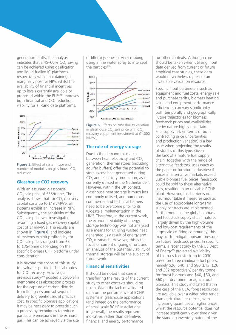
68
generation tariffs, the analysis indicates that a 45–60% CO2 saving can be achieved using gasification and liquid fuelled IC platforms respectively while maintaining a marginally positive NPV, whilst the availability of financial incentives up to levels currently available or proposed within the EU17,18 improves both financial and CO2 reduction viability for all candidate platforms.
Figure 5. Effect of system type and number of modules on glasshouse CO2 reduction
Figure 6. Effects on NPV due to variation in glasshouse CO2 sale price with CO2 recovery equipment investment at £1,000 k/MWe
Glasshouse CO2 recovery
With an assumed glasshouse CO2 sale price of £35/tonne, The analysis shows that for CO2 recovery capital costs up to £1m/MWe, all systems exhibit an increase in NPV. Subsequently, the sensitivity of the CO2 sale price was investigated assuming a fixed gas recovery capital cost of £1m/MWe. The results are shown in Figure 6, and indicate all systems exhibit profitability for CO2 sale prices ranged from £5 to £35/tonne depending on the specific biomass CHP platform under consideration.
It is beyond the scope of this study to evaluate specific technical routes for CO2 recovery. However, a previous study26a posited a polyolefin membrane gas absorption process for the capture of carbon dioxide from flue gases and subsequent delivery to greenhouses at practical cost. In specific biomass applications it may be necessary to precede such a process by techniques to reduce particulate emissions in the exhaust gas. This can be achieved via the use
of filters/cyclones or via scrubbing using a fine water spray to intercept the particles26b.
The role of energy storage
Due to the demand mismatch between heat, electricity and CO2 generation, thermal stores (including aquifer buffers) offer the potential to store excess heat generated during CO2 and electricity production, as is currently utilised in the Netherlands27. However, within the UK context, glasshouse heat storage is much less commonly utilised, and numerous commercial and technical barriers need to be overcome prior to its widescale implementation in the UK28. Therefore, in the current work, the economic viability of energy storage technology was not analysed as a means for utilising wasted heat generated as a result of energy and CO2 mismatch. However, this is the focus of current ongoing effort, and an analysis of the potential viability of thermal storage will be the subject of future work.
Financial sensitivities
It should be noted that care in transferring the results of the current study to other contexts should be taken. Given the lack of validated data on the performance of BCHP systems in glasshouse applications (and indeed on the performance of small scale BCHP installations in general), the results represent indicative, rather than definitive, financial and energy performance
for other contexts. Although care should be taken when utilising input data derived from current or future empirical case studies, these data would nevertheless represent an invaluable validation resource.
Specific input parameters such as equipment and fuel costs, energy sale and purchase tariffs, biomass heating value and equipment performance efficiencies can vary significantly both temporally and geographically. Future trajectories for biomass feedstock prices and availabilities are by nature highly uncertain. Fuel supply risk (in terms of both contracting price uncertainties and production variation) is a key issue when projecting the results of studies of this type. Given the lack of a mature fuel supply chain, together with the range of alternative feedstock uses (such as the paper or furniture industries) if prices in alternative markets exceed viable biomass fuel prices, feedstock could be sold to these alternative uses, resulting in an unviable BCHP plant. However, this barrier is not insurmountable if measures such as the use of appropriate long-term supply contracts are implemented. Furthermore, as the global biomass fuel feedstock supply chain matures (largely driven by the high-volume and low-cost requirements of the largescale co-firing community) this may act to mitigate upward pressure on future feedstock prices. In specific terms, a recent study by the US Dept. of Energy21i projected availability of biomass feedstock up to 2030 based on three candidate fuel prices, namely $20, $40, and $80 (£13, £26 and £52 respectively) per dry tonne for forest biomass and $40, $50, and $60 per dry tonne for agricultural biomass. This study indicated that in the case of the USA, forest resources are available over a wider price range than agricultural resources, with increasing quantities at higher prices, whilst the resource potential does not increase significantly over time given the standing inventory nature of the

140 The feasibility of biomass CHP as an energy and CO2 source for commercial glasshouses
69
Environment &
Sustainability
resource and how it is managed. Given these issues, any future users of the modelling tool should take care in verifying the accuracy of input data. To address uncertainties in such parameters, future development of the model would benefit from the application of probabilistic methods, such as Monte Carlo modelling or Bayesian network approaches, and work to this effect by the research team is ongoing29.
Conclusions
A modelling tool has been developed that facilitates the feasibility assessment of biomass CHP options for commercial glasshouse operators world-wide. By varying input parameters including local climactic data, energy/CO2 consumption profiles and tariffs, and biomass CHP cost and performance data, profitability assessments can be carried out on a location and application-specific basis in light of time and location-specific cost and energy tariff data along with any available support subsidies.
For the UK case study presented in this paper, the use of specific techno-economic input parameters shows that careful selection of the type and scale of BCHP platform for a specific glasshouse application is critical in order to realise project profitability. The majority of solid BCHP technologies are currently characterised by relatively high capital costs, and whilst liquid biofuel IC-based systems exhibits relatively low capital cost (and hence the shortest payback periods for the base case cost assumptions used in this study) this technology is also the most sensitive to fuel price fluctuations such as pertains at the current time.
For the case study illustrated in this work, sizing of the biomass CHP system to meet the average summer heat demand and electrical base load provides the most favourable techno-economic solution. For a typical 40,000m2 glasshouse, the
optimal base-case analysis shows that approximately 45% of annual heat demand, 90% of electricity demand and a 45–60% reduction in site CO2 emissions is achievable.
The analysis also suggests that the availability of a 25% capital grant can result in project profitability, due to offsetting relatively high capital costs for biomass CHP technology. An enhanced thermal energy generation tariff at a minimum price of £10/MW h provides significant benefit to biomass CHP viability by improving overall project profitability and reducing sensitivity to fuel price increases, whilst an enhanced electrical generation tariff of approximately £140/MW h provides increased forward economic visibility. It should be noted that these support levels are consistent with those currently being implemented in a number of EU states and beyond. Generation-based subsidies are best placed to contribute to reduced project risk if guaranteed over the long term, and are index-linked to inflation. When combined with additional strategies designed to help mitigate fuel price volatility such as long-term feedstock price contracting or project ‘joint-venture’ vehicles that include feedstock suppliers, overall project risk can be reduced significantly.
Although biomass CHP exhaust gases are not directly compatible for use in glasshouses, it may be feasible to utilise these for CO2 enrichment purposes with further treatment. By realising CO2 values of around £35/tonne (either via direct sale on site of via carbon trading mechanisms) an additional investment of up to £1 m/MWe for CO2 recovery equipment is feasible. Therefore, glasshouse CO2 demand provides a potential opportunity for the development of biomass gasification CHP with pre CO2 recovery, and warrants further investigation.
Glossary
ACH: air changes per hour
CHP: combined heat and power
EU: European union
FIT: feed-in tariff
IC: internal combustion
NPV: net present value
ORC: organic rankine cycle
UK: United Kingdom
IC: internal combustion

70
Acknowledgement
This paper was previously published in Applied Energy 96 (2012) 339–346, March 2012.
References
1. Aznar-Sánchez JA, Galdeano-Gómez E. Territory cluster and competitiveness of intensive horticulture in Almería (Spain). Open Geogr J 2011;4:103–14.
2. National Farmers. Union report – why horticulture matters; 2008. <http://www.whyfarmingmatters.co.uk/> [accessed 29.01.11].
3. Energy benchmarks and saving measures for protected greenhouse horticulture in the UK. The Carbon Trust, ECG091. pp. 8.(a) Chartered Institution of Building Services Engineers. Energy benchmarks – volume 46 of CIBSE TM. CIBSE; 2008.
4. Energy efficient production of high quality ornamental species. DEFRA project report HH1330, Department for environment food and rural affairs, UK; September 2003.
5. Besford RT. The greenhouse effect: acclimation of tomato plants growing in high CO2, photosynthesis and ribulose-1, 5-bisphosphate carboxylase protein. J Exp Bot 1990;41:925–31.
6. Nederhoff E. Open and closed buffer systems for heat storage. Grower 2004;59:41–2.
7. Sethia VP, Sharma SK. Experimental and economic study of a greenhouse thermal control system using aquifer water. Energy Convers Manage 2007;48:306–19;
a. Eriksson G, Kjellstrom B. Assessment of combined heat and power (CHP) integrated with wood-based ethanol production. Appl Energy 2010;87(12):3632–41.
8. Keppo I, Savola T. Economic appraisal of small biofuel fired CHP plants. Energy Convers Manage 2007;48:1212–21.
9. Wetterlund E, Söderström M. Biomass gasification in district heating systems – the effect of economic energy policies. Appl Energy 2010;87:2914–22;
a. Wood SR, Rowley PN. A techno-economic analysis of small-scale biomassfuelled, combined heat and power for community housing. Biomass Bioenergy 2011;35:3849–58;
b. Bram S, DeRuyck J, Lavric D. Using biomass: a system perturbation analysis. Appl Energy 2009;86(2):194– 201.
10. Chau J et al. Techno-economic analysis of wood BM boilers for the greenhouse industry. Appl Energy 2009;86:364–71.
11. Adams S, Langton A. Energy management in protected cropping: manipulation of glasshouse temperature. DEFRA factsheet 06/09; 2009. <http://www.hdc.org.uk/assets/pdf/33209023/10706.pdf> [accessed 2.02.10].
12. Bot G. Developments in indoor sustainable plant production with emphasis on energy saving. Comput Electron Agric 2001;30:151–65.
13. Worley J. Greenhouses, heating, cooling and ventilation. Univ Georgia Bull2009;792:1–10.
14. Wass SN, Barrie IA. Application of a model for calculating glasshouse energy requirements. Energy Agric 1984;3:99–108.
15. Chartered Institution of Building Services Engineers. CIBSE Guide J; 2002. Table 5.36. ISBN 9781903287125.
16. O’Flaherty T, Cochran R. Determination of glasshouse heat requirements from temperature and wind records. Acta Hortic 1976;46:33–8.
17. Blom TJ et al., Carbon dioxide in greenhouses; 2002. OMAF. ISSN 1198-712X.

140 The feasibility of biomass CHP as an energy and CO2 source for commercial glasshouses
71
Environment &
Sustainability
18. Improving the energy efficiency of protected cropping in winter through the use of low intensity, long-day lighting. DEFRA project report HH3603SPC. Department for Environment Food and Rural Affairs, UK; December 2003. p.13–4.
19. Schwab E. Technologies for syngas purification. BASF presentation for IEA task 33 meeting; May 2009. slide 6.
20. Dong L, Liu H, Riffat S. Development of small-scale and micro-scale biomassfuelled CHP systems – a literature review. Appl Therm Eng 2009;29:2119–26.
21. Forestry Commission Biomass Energy Centre information sheet no. 4: combined heat and power. <http://www.biomassenergycentre.org.uk/pls/portal/docs/> [accessed 29.01.11].;
a. Biomass Combined Heat and Power Catalog of Technologies. Report prepared for US. Environmental Protection Agency combined heat and power partnership, September 2007; July 2011. <http://www.epa.gov/ chp/documents/biomass_chp_catalog.pdf>.;
b. Bakos GC, Tsioliaridoua E, Potolias C. Technoeconomic assessment and strategic analysis of heat and power cogeneration (CHP) from biomass in Greece. Biomass Bioenergy 2008;32(6):558–67;
c. Keppoa I, Savolab T. Economic appraisal of small biofuel fired CHP plants. Energy Convers Manage 2007;48(4):1212–21;
d. Pantaleo A, Pelleranoa A, Caronea MT. Potentials and feasibility assessment of small scale CHP plants fired by energy crops in Puglia region (Italy). Biosyst Eng 2009;102(3):345–59;
e. ‘Biomass prices in the heat and electricity sectors in the UK’. Report for the UK Department of Energy and Climate Change, January 2010, Ref: URN 10D/546; November 2011. <http://www.decc.gov.uk/assets/ decc/consultations/rhi/132-biomass-price-heat-elec-e4tech.pdf>.;
f. McKenneya W, Yemshanova D, Fraleigha S, Allena D, Pretob F. An economic assessment of the use of short rotation coppice woody biomass to heat greenhouses in southern Canada. Biomass Bioenergy 2011;35(1):374 84;
g. Sami MK, Annamalai K, Wooldridge M. Co-firing of coal and biomass fuel blends. Prog Energy Combust Sci 2001;7:171–214;
h. Boundy B, Diegel SW, Wright SWL, Davis SC. Biomass energy data book: edition 4. Report #ORNL/TM- 2011/446 by the Oak Ridge National Laboratory for the Office of the Biomass Program, US Department of Energy; November 2011. <http://cta.ornl.gov/bedb/pdf/BEDB4_Full_Doc.pdf> [prepared September 2011].;
i. US Department of Energy. 2011 US billion-ton update: biomass supply for a Bioenergy and Bioproducts Industry. In: Perlack RD, Stokes BJ, Leads. ORNL/TM-2011/224. Oak Ridge National Laboratory, Oak Ridge, TN; November 2011. 227p. <http://www1.eere.energy.gov/biomass/pdfs/billion_ton_update.pdf>.;
j. Kalt G, Kranzl L. Assessing the economic efficiency of bioenergy technologies in climate mitigation and fossil fuel replacement in Austria using a techno-economic approach. Appl Energy 2011;88(11):3665–84.
22. Directive 2004/8/EC of the European Parliament on the promotion of cogeneration based on a useful heat demand in the internal energy market and amending Directive 92/42/EEC.
23. Westner G, Madlener R. The benefit of regional diversification of cogeneration investments in Europe: a mean–variance portfolio analysis. Energy Policy 2010;38:7911–20.
24. Klein A, Pfluger B, Held A, Ragwitz M, Resch G. Evaluation of different feed-in tariff design options: Best practice paper for the international feed-in cooperation, 2nd ed. Berlin (Germany): BMU; 2008. http://www.feed-incooperation. org/wDefault_7/wDefault_7/download-files/research/best_practice_paper_2nd_edition_final.pdf> [accessed 01.11.10].
25. del Río Gonzalez P. Ten years of renewable electricity policies in Spain: an analysis of successive feed-in tariff reforms. Energy Policy 2008;36:2917–29.
26. Consultation on Renewable Electricity Financial Incentives 2009, DECC, July 2009, pp.83 [cost ref p1] Department of Trade & Industry. Impact of banding the Renewables Obligation – Costs of electricity production. April 2007. URN 07/948.;

72
a. Feron PHM, Jansen AE. The production of carbon dioxide from flue gas by membrane gas absorption. Energy Convers Manage 1997;38:S93–8;
b. Karellas S, Karl J, Kakaras E. An innovative biomass gasification process and its coupling with micro turbine and fuel cell system. Energy 2008;33:284–91.
27. Pietola K, Lansink AO. Modelling energy saving technology choices in Dutch glasshouse horticulture. Econ Sustain Energy Agric: Econ Environ 2003;24:41–55.
28. Plackett C. ’Green’ glasshouse technologies not yet a realistic option. Horticulture Week; 10 April, 2008. <http://www.hortweek.com/news/802355/> [accessed 11.02.11].
29. Wilson DM, Rowley PN, Watson SJ. Utilizing a risk-based systems approach in the due diligence process for renewable energy generation. IEEE Syst J 2011;5(2):223–32.

140 The feasibility of biomass CHP as an energy and CO2 source for commercial glasshouses
73
Environment &
Sustainability
Electricity Demand
Electricity demand profiles
Glass Internal Temperature Set-point
The glasshouse internal temperature set point is changed throughout the day, a typical set point temperature profile for tomatoes is given in Table 2 For tomato crops the temperature is dropped towards the end of the day around sunset to encourage fruit size. The figures in Table 2 have been used in the heat demand model.
Appendix
Technical considerations
Heat Demand
Glasshouse Air Change Rate
Typical air change rates with roof vents closed are giving in the Table 1.
Glass Construction ACH
New construction 0.75 to 1
Old construction, good maintenance
1.0 to 2.0
Old construction, poor maintenance
2.0 to 4.0
Relative Time Hrs Temperature °C
Sunrise -2Hrs 16
Sunrise 18
Sunrise + 2Hrs 20
Other daylight Hrs 23
Sunset -4Hrs 21
Sunset 15
Sunset +4Hrs 17
Boiler efficiency
Gas p/therm η=80% η=85% η=90%
20 8.53 8.03 7.58
30 12.80 12.04 11.37
40 17.06 16.06 15.17
50 21.33 20.07 18.96
60 25.59 24.09 22.75
70 29.86 28.10 26.54
Glasshouse Heating System2
Due to the demand mismatch between heat and CO2 generation, glasshouses use large water tanks often referred to as buffers to store the heat generated during CO2 production. The heat storage tank was developed in the Netherlands in the 1980’s for glasshouse applications. The buffer systems can be open or closed; the closed buffer system was designed to assist CO2 production only compared to the more modern open buffer system which can also be used for energy management. With an open buffer system it is possible to load and unload the buffer at the same time; this is achieved through the control of pumps with variable speed drives. A mixing valve at the boiler or CHP ensures that the return temperature and hence flow temperature for a given temperature lift meets the correct requirement. The temperature gradient within the buffer is measured to determine the current amount of heat storage. An overview of a typical open buffer system is shown in Figure1.
Table 1. Natural Air Changes Per Hour1
Table 2. Glasshouse Internal Temperature Set Point10
Table 3. Cost to Produce 1MWh of Heat form Natural Gas
Natural Gas Heating Costs
Heat Demand Profiles
Figure 1. Glasshouse Open Buffer System
Figure 2. Hourly Heat Demand W/m2 for Each Month
Figure 3. Monthly Heat Demand, 40,000m2 Glasshouse
Figure 4. Hourly Electrical Demand W/m2
Figure 5. Monthly Electricity Demand, 40,000m2 glasshouse
CO2 Demand
Photosynthesis
Photosynthesis is a chemical process that uses the suns energy to convert CO2 and water into energy such as glucose. The overall chemical reaction for glucose synthesis via photosynthesis is shown below:
6C02 + 6H2O + Light Energy C6H12O6 + 6O2
The rate of CO2 demand by the glasshouse crop increases with increasing PAR, and also increases with increasing CO2 in the glasshouse atmosphere. Air temperature,

74
cleaned using Selective Catalytic Reduction (SCR) with a reducing agent such as Urea to reduce the NOx levels and Oxidation Catalyst to reduce any unburnt hydrocarbons i.e. Carbon Monoxide and Ethylene. Ethylene is phytotoxic and CO is toxic to humans.4 A typical natural gas CHP arrangement with exhaust gas cleaning for glasshouses is shown in Figure 8. The use of a catalyst is possible due to minimal variations in the natural gas quality and low particulate emissions. The use of the condenser on the CHP as well as reducing the moisture of the exhaust gas helps to increase the concentration of CO2/Nm3 allowing a higher concentration of CO2/Nm3 to enter the glasshouse compared to CO2 being supplied by boilers.
Sources of CO2
Each MWh of gas burned directly produces a proportionate amount of CO2. Under complete combustion, methane (the main component of natural gas) produces CO2, water and heat as shown below:4
CH4+ 2O2 CO2+ 2H2O + Heat
One MWh of natural gas burned will produce 184kg of CO2 based on the gross calorific value (obtained from DEFRA June 2009 conversion factors3). Moisture needs to be removed from the exhaust gas as it can cause mould and fungus.
Cost of CO2 Produced from Natural Gas
The typical cost (excluding equipment cost) per tonne of CO2 produced by boilers with natural gas burners is shown in Table 5.
relative humidity and water stress also contribute to the rate of CO2
demand. The concentration of CO2 within the glasshouse will also depend on the natural and forced ventilation. In a well sealed glasshouse CO2 concentration can drop below outside ambient levels1 Without CO2 enrichment, ventilation can help increase the CO2 concentration closer to ambient levels but at the cost of losing heat. With CO2 enrichment, the CO2 will be diluted with the outside atmosphere when the glasshouse vents are opened to help control the temperature. A lower CO2 concentration is maintained when venting is being used to cool the glasshouse. Table 4 below shows the estimated rate of CO2 required to maintain set CO2 levels in the glasshouse. These figures assume high light level conditions and minimal air changes. This will of course vary depending on the glasshouse ACH, light intensity, type of crop and growing strategy.
CO2 level (ppm) CO2 Supply Rate
500 70 to 90 Kg/Ha/Hr
900 170 to 190 Kg/Ha/Hr
1,300 250 to 350 Kg/Ha/Hr
Table 4. Rate of CO2 Required to Maintain Set CO2 Levels1
Table 5. Cost of CO2 Production Using Boilers with Natural Gas Burners
CO2 Demand Profiles
Figure 6. Glasshouse Open Buffer System
Figure 7. Monthly CO2 Demand, 40,000m2 Glasshouse
Figure 8. Typical Arrangement of Natural Gas Fired CHP with Exhaust Gas Cleaning
Gas p/therm Gas £/MWh CO2 £/tonne
20 6.82 37.17
30 10.24 55.76
40 13.65 74.34
50 17.06 92.93
60 20.47 111.52
70 23.88 130.11
Natural Gas CHP
Natural gas can also be combusted in a reciprocating engine to form part of a CHP plant, although the exhaust gas produced by the engine is not suitable for direct supply to the glasshouse. It must first be
Biomass combustion
The combustion of biomass takes place in three stages, Drying (0 to 200°C), Pyrolysis (200 to 400°C) and Oxidation (400 to 1000°C).
The complete combustion of biomass with a chemical composition CxHyOz and oxygen is shown below;5
CxHyOz+(x + y/4 - z) O2 xCO2+ y/2 H2O+ Energy
Biomass mainly contains cellulose, hemi cellulose and lignin. Taking cellulose as a component on its own, the complete combustion would be represented as follows: 4
C6H10O5+ 6O2 6CO2+5H2O+Heat
It can be seen that under complete combustion this reaction produces water, carbon dioxide and heat.

140 The feasibility of biomass CHP as an energy and CO2 source for commercial glasshouses
75
Environment &
Sustainability
System 2 - Biofuel (vegetable oil) using compression ignition engine by Living Power
Virgin vegetable oil or processed used cooking oil can be combusted in a modified compression ignition engine. The fuel price is higher compared to biomass and more susceptible to price variations, however capital costs are lower compared to biomass systems. Heat can be recovered from engine jacket water, oil cooler, intercooler and exhaust.
The net produce of air gasification is found to be7
C6H10O5 + O2 CxHz + CnHmOy + CO + H2 + Heat
Typically the gas produced will contain a mixture of different components and this will depend on the feedstock and gasifier used. For heat and power generation the gas produced is then used in a spark ignition engine. The typical basic exhaust gas emission data was obtained from an operational plant in Austria and is shown in Table 7.
If cellulose has an energy value of 19GJ/t, using the atomic weights of each component,
162 + 192 264 + 90 + Heat
Under complete combustion 1MWh of energy provided by cellulose would produce 308kg CO2. Per MWh of energy released biomass will provide a higher volume of CO2 compared to natural gas. Under real conditions however, complete combustion does not occur, slightly higher concentrations of CO2 and other elements will be produced depending on the actual fuel composition and combustion. Basic emission data was also obtained from an compression ignition engine operating on Soya oil, this data is shown in Table 6.
Table 6. Emissions from Compression Engine Operating on Soya Oil6
Table 7. Exhaust Gas Composition from Engine Operating on Syngas @ 5% Oxygen8
Figure 9. Biomass CHP, Gasifier with IC engine
Figure 10. Biofuel CHP using Compression Ignition Engine
Figure 11. Biofuel CHP using Direct Combustion with ORC
Contamination Concentration
Sulphur Dioxide [SOx] 153 ppm
Hydrocarbons [CxHy] unknown
Carbon Monoxide [CO] 873 ppm
Nitrogen Oxide [NOx] 1913 ppm
Particulates 5.3 mg/m3
Component Concentration
NOx ppm 372
CO ppm 2920
Biomass Gasification
Gasification is a thermal process of converting dry solid fuels into gaseous ones under partial oxidation conditions. The combustible gas produced is referred to as producer or synthesis gas (syngas) depending on the oxidiser used e.g. oxygen or steam. Gasification has certain advantages that cannot be achieved through direct combustion of the material, the main advantage being that the gas can be used in an internal combustion engine to then produce electricity and heat. Gasifiers come in many different shapes and forms, each with their own advantages and disadvantages for particular applications.
Air gasification can be expressed in three stages;
Oxidisation Pyrolysis Gasification
This shows that the emissions levels as they stand would be unsuitable for glasshouse applications. Other unburnt hydrocarbons would also need investigating.
Conversion Technologies
System 1 - Biomass Gasifier with IC engine by Alfagy / Enercarb
Solid dry biomass is converted in to a combustible gas by heating in a reduced oxygen environment. Gasifiers can take many different shapes and forms. The gas needs to be cleaned to remove particulates and other contaminants before it is combusted in a modified or specifically designed spark ignition engine. Heat can be recovered from the gas produced and from the engine jacket water, oil cooler, intercooler and exhaust.
System 3 - Direct Biomass combustion with ORC by Turboden
Solid biomass is combusted directly and used to heat a secondary organic fluid and drive a small turbine. This is called the Organic Rankine Cycle and is similar to a traditional steam turbine system, but the working fluid has a much lower boiler point and can therefore achieve higher efficiencies in smaller systems.
System 4 - Combined cycle biomass gasification CHP by Babcock & Wilcox Volund
The combined cycle biomass gasification CHP is a further improvement on the standard gasification with IC engine and is specifically being developed by one manufacturer. The benefits

76
Triad % Share 95 %
Waste Disposal £10/Tonne
Project Period 15 Years
Inflation Rate (RPI) 3 %
Discount Rate 10 %
Loan interest rate 9 %
to reduce the particulate emissions in the exhaust gas, this can be via a wet or dry process. The dry process involve the use of filters / cyclones, these can be in the form of bag filters or electrostatic filters and in the wet process the exhaust gas is scrubbed using a fine water spray to intercept the particles. Scrubbing also has the advantage of SOx and NOx particle removal but there is the added expense of water treatment. Deactivation of SCR can be caused by blinding over of the catalyst e.g. by particulate emissions, pore condensation and poisoning.10
Biomass Gasification
Water Gas Shift chemical reaction:
CO+H2O CO2+ H2
Economic considerations
Modelling assumptions
are improved electrical efficiency and improved combustion of CO components. The tar that has to be scrubbed out from the gas still contains energy and is separated and burnt with at a high stoichiometric temperature in the exhaust gas of the IC engine, this ensures that excess CO from the IC engine is burnt out. The exhaust gas then passes through a heat recovery steam generator, the steam is then used to drive a steam generator to generate electricity providing the combined cycle. The minimum plant size is 4MWe. The expected exhaust emission data is shown in Table 8.
Component Concentration
NOx mg/Nm3 250
SO2 mg/Nm3 10
CO mg/Nm3 150
TOC mg/Nm3 30
Table 8. Exhaust Gas Composition From Combined Cycle Gasification CHP9
Table 9. Baseload Modelling assumptions
System 5 - Direct Biomass combustion with Externally Fired Air Turbine by Talbots
Solid biomass is combusted directly and used to heat air via a heat exchanger, the heated air is then expanded through a turbine which is used to generate electricity.
Figure 12. Biofuel CHP using direct combustion with Externally Fired Air Turbine
Method of Possible Biomass / Biofuel CHP CO2 Recovery
Biomass & Biofuel Combustion
Secondary techniques can be used
ParameterBase Case Value
Solid Biomass Heating Value
19 GJ/Tonne
Solid Biomass Heating Cost £50/ODT
Liquid Biofuel Heating Value
37 GJ/Tonne
Liquid Biofuel Heating Cost £500/Tonne
Availability 90%
Electricity Base load Export Price
45 £/MWh
Electricity Peak load Export Price
50 £/MWh
Electricity Onsite Sale Price 55 £/MWh
Electricity Import Price 60 £/MWh
Gas Price 47p/Therm
Heat Sale Price 20 £/MWh
Glasshouse CO2 Sale Price 35 £/Tonne
CCL Electricity 4.70 £/MWh
CCL Gas 1.64 £/MWh
RO 3.60 £/MWh
ROC 53 £/MWh
LEC 4.70 £/MWh
Triad 22 £/kWh
ROC % Share 95 %
LEC % Share 95 %
Gas and Power prices obtained from www.heren.com/ on the 6th August 2009. ROC price obtained from E-ROC website www.eroc.co.uk, price correct on 7th July 2009. Biofuel referred to in the report is Vegetable oil (Soya oil). The Biofuel cost was obtained from Living Power and M.W. Beer in August 2009, the price had increased to £525 in September 09 indicating the variations that can occur in vegetable oil. Biomass referred to in the report is woodchip, prices were obtained from Manco Energy and AHS Energy in August 2009. It should be noted that vegetable oil is traded as a commodity and can vary on a daily basis. Biomass and Biofuel supply will also be subject to the site location and the supply should be investigated before a project is developed.
Loan Rate Sensitivity
Using the modelling assumptions with no capital grant, the sensitivity of the NPV was tested by adjusting the loan interest rate between 0 to 15%. The results are shown in figure 13. System 2 has the least sensitivity, still being able to maintain a positive NPV at a loan interest rate of 15%. Systems 1,3 & 5 have very similar sensitivity to loan interest rate and the NPV becomes negative when the loan interest rate approaches the range 7 to 11%. System 4 can achieve a positive NPV up to a loan interest rate of 13%.

140 The feasibility of biomass CHP as an energy and CO2 source for commercial glasshouses
77
Environment &
Sustainability
currently have a value of £4.70/MWh and can be sold into the market.
Renewable Obligation
The Renewable obligation is a mechanism in the UK market to encourage the use of renewable electricity generation and was updated in April 2009. Depending on the technology type, each MWh of renewable electricity generated will obtain a number of Renewable Obligation Certificates (ROCs). These ROCs have a value and can then be sold into the market and / or used to meet the owners own renewable obligations. The value of ROCs can be obtained at www.eroc.co.uk. Commercial users of electricity currently have to pay a Renewables Obligation (RO) on electricity they use from a non renewable source. The rate is currently £3.60/MWh which is used to support the ROC mechanism. Good quality Biomass / Biofuel CHP as defined by the UK CHPQA scheme will obtain 2 ROC’s for each MWh generated, if a scheme fails to be good quality due to excess heat not being used, 1.5 ROC’s per MWh generated will be obtained. Full details of the Renewables Obligation Order 2009 can be found at www.opsi.gov.uk, the direct link is http://www.opsi.gov.uk/si/si2009/pdf/uksi_20090785_en.pdf.
Operating base load on an annual basis, this system would only attract 1.5 RCOs/MWh due to a large amount of heat that would be dumped in the summer months. However, if the operating regime is changed to a peak profile in months 5 to 9, the heat generated matches the demand much better and will continue to maintain good quality
Operating regime with System 2 (Biofuel)
As Biofuel CHP has much greater flexibility compared to biomass CHP, it can be operated at base or peak load. An analysis was performed to look at the effects of installing a higher MWe system but operating a peak profile in the summer and a baseload profile in the winter to better match the heat demand and maintain good quality CHP. Figure 14 shows the typical glasshouse demands and the generation from ten system 2 modules operating a peak profile in months 5 to 9 and a baseload profile in all other months.
Figure 13. Sensitivity to Loan Interest Rate
Figure 15. 40,000m2 Glasshouse Demand and Generation from 16x System 2 (Biofuel) Modules. Operating a Peak Profile in Months 5 to 9 and Baseload all Other Months. Heat Generation is Better Matched to Heat Demand
Figure 14. 40,000m2 Glasshouse Demand and Generation from 10x System 2 (Biofuel) Modules. Operating a Peak Profile in Months 5 to 9 and Baseload all Other Months
CHP status attracting 2 ROCs/MWh. A further example of using 16 modules of system 2 operating a peak profile in the summer is shown in Figure 15. In the winter this closely matches the winter heat demand meaning there is less shortfall heat that has to be supplied from boilers.
CHPQA
A CHP scheme must obtain a Quality Index (QI) score above 100 under the UK CHP Quality Assurance scheme to maximise the benefit from Levy Exemption Certificates and Renewable Obligation Certificates. The CHPQA scheme in the UK has been operating since 2001. The QI score calculation is based on the electrical efficiency of the CHP and its useful heat output, therefore to maximise the QI score there must be a use of the heat generated. The QI calculations depend on the technology and size of system installed. The formulas are readily available in the CHPQA guidance notes at www.chpqa.com.
A Climate Change Levy (CCL) is charged on all fossil fuels in the UK such as natural gas and electricity. CCL on electricity is currently £4.70/MWh. Good Quality CHP has the benefit of being CCL exempt and a Levy Exemption Certificate (LEC) is obtained for every MWh generated from good quality CHP. LEC’s

78
Bibliography
The following papers, guides and studies have all been consulted throughout the project and provide useful information relevant to various aspects of biomass fuelled CHP.
1. D.L Critten and B.J. Bailey, “A review of greenhouse engineering developments during the 1990s”, Agricultural and Forestry Meteorology, Vol. 122, 2002, pp. 1-22.
2. K. Popovski, “Factors Influencing Greenhouse Heating and Geothermal Heating Systems”, Geothermics, Vol 17, No1, 1988, pp. 173-189.
3. Otto Frøsig Nielsen, “Climate Computer algorithms for Peak Shaving of Greenhouse heating demand”, Computers and Electronics in Agriculture, Vol. 13, 1995, pp. 315-335.
4. S.N Wass and I.A Barrie, “Application of a Model for Calculating Glasshouse Energy Requirements”, Energy in Agriculture, Vol. 3, 1984, pp. 99-108.
5. T.O’Flaherty & R.Cochran, “Determination of glasshouse heat requirements from temperature and wind records”, Symposium on Greenhouse Design and Environment, Vol. 46, pp. 33-54.
6. B. Ozkana, A. Kurklub and H. Akcaoza, “An input–output energy analysis in greenhouse vegetable production:a case study for Antalya region of Turkey”, Biomass and Bioenergy, Vol. 26, 2004, pp. 89 – 95.
7. G. Houter, “Simulation of CO2 consumption, heat demand and crop production of greenhouse tomato at different CO2 strategies”, CO2 in Protected Cultivation, Vol. 268, 1990, pp. 157-163.
8. J.G Hare, B. Norton and S.D. Probert, “Design of greenhouses: Thermal Aspects”, Applied Energy, Vol. 18, 1984, pp. 49-82.
9. D.W. Hand, J.D. Postlethwaite and M.A. Hannah, “Carbon dioxide generation from low-sulphur kerosene”, J.agric. Engng Res., Vol. 20, 1975, pp. 89-97.
10. S. Karellas, J.Karl and E.Kakaras, “An innovative biomass gasification process and its coupling with micro turbine and fuel cell systems”, Energy, Vol. 33, 2008, pp. 284 291.
11. A.A. Rentizelas, I.P. Tatsiopoulos and A. Tolis, “An optimization model for multi-biomass tri-generation energy supply”, Biomass and Bioenergy, Vol. 33, 2009, pp. 223-233.
12. S. N. Uddin and L. Barreto, “Biomass-fired cogeneration systems with CO2 capture and storage”, Renewable Energy, Vol. 32, 2007, pp. 1006-1019.
13. A. Marbe and S.Harvey, “Opportunities for integration of biofuel gasifiers in natural-gas combined heat-and-power plants in district-heating systems”, Applied Energy, Vol. 83, 2006, pp.723-748.
14. A. Marbe, S.Harvey and T.Berntsson, “Technical, environmental and economic analysis of co-firing of gasified biofuel in a natural gas combined cycle (NGCC) combined heat and power (CHP) plant”, Energy, Vol. 31, 2006, pp. 1614-1631.
15. M. Lapuerta et al, “Diesel emissions from biofuels derived from Spanish potential vegetable oils”, Fuel, Vol. 84, 2005, 773-780.
16. A. Kurklu, “Energy storage applications in greenhouses by means of phase change materials (PCMs) : a review”, Renewable Energy, Vol. 13, No. 1, 1998, pp. 89-103.
17. Hugo H. Rogers, G. Brett Runion & Sagar V. Krupa, “Plant Responses to Atmospheric CO2 Enrichment with Emphasis on Roots and the Rhizosphere, Environmental Pollution, Vol. 83, 1994, PP. 155-189.
18. D. P. Aikman, “A Procedure for Optimizing Carbon Dioxide Enrichment of a Glasshouse Tomato Crop”, J.agric. Engng Res., Vol. 63, 1996, pp. 171-184.
19. I. Keppo and T. Savola, “Economic appraisal of small biofuel fired CHP plants”, Energy Conversion and Management, Vol. 48, 2007, 1212-1221.
20. J. Chau et al, “Techno-economic analysis of wood biomass boilers for the greenhouse industry”, Applied Energy, Vol. 86, 2009, pp. 364-371.

140 The feasibility of biomass CHP as an energy and CO2 source for commercial glasshouses
79
Environment &
Sustainability
21. R. T. Besford et al, “The Greenhouse Effect: Acclimation of Tomato Plants Growing in High CO2, Photosynthesis and Ribulose-1, 5-Bisphosphate Carboxylase Protein”, Journal of Experimental Botany, Vol. 41, 1990, pp. 925-931.
22. E. Nederhoff, “Open and Closed Buffer Systems for Heat Storage”, The Grower, Vol.59, 2004, pp.41-42.
23. J.Worley, “Greenhouses, Heating, Cooling and Ventilation”, The University of Georgia, Bulletin 792, 2009, pp.1-10.
24. Dr. P. “Tans Mauna Loa CO2 annual mean data”, NOAA/ESRL, www.esrl.noaa.gov/gmd/ccgg/ trends/.
25. “Energy Benchmarks and Saving Measures for Protected Greenhouse Horticulture in the UK”, The Carbon Trust, ECG091, pp.8.
26. T.J Blom et al, “Carbon Dioxide in Greenhouses”, OMAF, ISSN 1198-712X, 2002.
27. S.V Loo et and J.Koppejan, “The Handbook of Biomass Combustion & Co-firing”, EarthScan, 2007, pp. 308-310,334.
28. E. Schwab, “Technologies for Syngas Purification”, BASF Presentation for IEA Task 33 Meeting, May 2009, Slide 6.
29. T.Elsenbruch, “Latest Developments in the Use of Wood Gas in Gas Engines” GE Jenbacher Presentation at IDGTE Toronto, June 2008, Slide 33.
30. M. Kasper, “Syngas Conditioning by Lurgi Rectisol”, Lurgi Rectisol Presentation for IEA Task 33 Meeting, May 2009, Slide 19.
31. “Consultation on Renewable Electricity Financial Incentives 2009”, DECC, July 2009, pp.83.
32. Defra’s greenhouse gas (GHG) conversion factors for company reporting @ http://www.defra.gov.uk/environment/business/reporting/conversion-factors.htm.
33. S.Wood & P.Rowley, “The Feasibility of Small-Scale, Biomass-Fuelled Combined Heat and Power for Community Housing”, CREST.
34. http://www.biomassenergycentre.org.uk.
35. http://www.gastechnology.org.
36. http://www.gasnet.uk.net.
37. https://www.chpqa.com.
38. http://www.crophouse.co.nz.
Companies Contacted
The following companies have been contacted during the project and I am grateful for any information provided.
1. Zero Point Clean Tec, USA
2. AFC Energy, UK
3. Clarke Energy, UK
4. PRM Energy, USA
5. Joule Power, UK
6. Biomass CHP, UK
7. Mawera, UK
8. Living Power, UK
9. Baltic Energy Group, Denmark
10. Babcock & Wilcox Vølund, Denmark
11. Advanced Plasma Power, UK
12. Looije Agro Technics, Netherlands

80
13. Schmitt Enertec, Germany
14. Steuler Analgenbau, Germany
15. Wight Salads.
Appendix References
1. J.Worley, “Greenhouses, Heating, Cooling and Ventilation”, The University of Georgia, Bulletin 792, 2009, pp.1-10.
2. E. Nederhoff, “Open and Closed Buffer Systems for Heat Storage”, The Grower, Vol.59, 2004, pp.41-42.
3. DEFRA Conversion Factors http://www.defra.gov.uk/environment/business/reporting/conversion-factors.htm.
4. J. Chau et al, “Techno-economic analysis of wood biomass boilers for the greenhouse industry”, Applied Energy, Vol. 86, 2009, pp. 364-371.
5. A.V. Bridgwater, “Renewable Fuels and Chemicals by Thermal Processing of Biomass”, Chemical Engineering Journal, Vol 91, 2003, pp87-102.
6. Provided verbally by Living Power Ltd.
7. M.A. Azam et al, “Construction of a Downdraft Biomass Gasifier”, Journal of Mechanical Engineering, Vol ME37, 2007, pp.71-73.
8. Holzgas Gussing – Exhaust Gas and Pollutant Emissions from GE Jenbacher 620 – Provided by Clarke Energy.
9. Babcock & Wilcox Vølund gasification information sheet provided by Baltic Energy Group.
10. V Loo et and J.Koppejan, “The Handbook of Biomass Combustion & Co-firing”, EarthScan, 2007, pp. 308-310,334.
11. Provided verbally by Wight Salads Ltd.

Highw
ay Netw
ork Managem
ent141
81
Simon R. Nuttall
Managing Consultant
Management Consultants
Atkins
Seosamh B. Costello
Senior Lecturer, Department of Civil and Environmental Engineering
The University of Auckland
Richard Arrowsmith
Planning and Performance Group Manager
Highways Agency
James E. Powell
Efficiency & Performance Manager
Highways & transportation
Atkins
IntroductionBackground
The Highways Agency, an executive agency of the UK Department for Transport, is the body responsible for the operation, maintenance and improvement of the strategic road network in England on behalf of the Secretary of State for Transport. The strategic road network is made up of England’s motorways and all-purpose trunk roads. Valued at over £87 billion, the network carries one-third of all road traffic in England and two-thirds of all heavy freight traffic (www.highways.gov.uk).
Although the scope of the Highways Agency is national, the country is divided into seven operational regions: eastern, east midlands, north east, north west, south east,
Performance management framework for managing agent contractorsAbstract
This paper describes a performance management framework for managing agent contractors working on the UK Highways Agency trunk road network. At the core of the framework is a performance hierarchy which links the operational activities carried out by the managing agent contractors with the key business outcomes of the Highways Agency. The hierarchy is weighted to allow the relative importance of hierarchy elements to be accurately represented, and to avoid the default position whereby everything is considered equally important. The framework utilises performance flags to visually represent performance at higher levels in the hierarchy, based on red, amber and green scores assigned at the lowest level in the hierarchy. The performance flags have the ability to show the detail behind a performance score, whereby a proportion of the flag will be green, a proportion amber and the remainder red depending on the frequency and weightings assigned to the lower contributing levels in the hierarchy. In an effort to reduce subjectivity in performance scoring, a scoring guidance document has been prepared in support of the framework. The performance management and continual improvement process is carried out on a monthly cycle akin to the standard improvement cycle of ‘plan, do, check, act’. The main benefits of implementing this process include reduced subjectivity, thereby allowing comparability between managing agent contractors, increased visibility, increased dialogue, targeted evidence-based decision making and auditability All of the above will help to drive improved effectiveness and efficiency in the delivery of managing agent contracts.
south west and west midlands. Each operational region is further broken down into areas, of which there are 12 in total. Highway maintenance and improvement in each of these areas is managed by a managing agent contractor (MAC) under contract to the Highways Agency.
Performance management
The performance of the MACs is managed by the Highways Agency through their area teams following a standard improvement cycle of ‘plan, do, check, act’ using measures to identify levels of performance and enable benchmarking as a means of driving improvement in operational delivery. These performance measures are set out in the motivating success toolkit (MST) developed specifically

82
Finally, taking sub-lever 1.2.1 as an example, three aspects contribute to it, namely 1.2.1.a Programming schemes, 1.2.1.b Delivering schemes and 1.2.1.c Monitoring scheme outcomes.
The descriptions and reference numbers for each of the levers, sub-levers and aspects have been obtained from the latest version of the Toolkit. Full descriptions of the aspects are also available in the Toolkit, abbreviated versions being used in the performance hierarchy due to space limitations.
The fully developed performance hierarchy for MACs, in the form of a performance hierarchy poster, is included as supplementary data with the online version of this paper.
Performance scoring
The scoring of performance in the MAC performance management framework is conducted at aspect level, this being the lowest level of standardisation in the Toolkit. Every aspect receives a red, amber or green score, hereafter referred to as a RAG score, depending on performance. Where no data have been submitted a fourth option is available, which is represented by the colour white. This ensures that failure to submit performance data is clearly evident and prevents erroneous assumptions being made about missing data.
Scoring guidance
In an effort to reduce the subjectivity in performance scoring, as well as the variability in locally agreed evidence provided in support of the performance scores, a scoring guidance document has been prepared in support of the framework (Highways Agency, 2010).
The guidance document provides detailed scoring guidance for each and every aspect, grouped by outcome. The scoring guidance also details what MACs need to demonstrate to justify their scores and lists the associated evidence that needs to be provided.
Performance management framework
Performance hierarchy
At the core of the MAC performance management framework is a performance hierarchy which shows how the operational activities of a MAC align with the key business outcomes of the Highways Agency.
The structure of the hierarchy is demonstrated schematically in Figure 1. The outcomes sit at the top of the hierarchy, a number of levers contribute to each outcome, a number of sub-levers contribute to each lever and, finally, a number of aspects contribute to each sub-lever.
The Highways Agency’s key business outcomes form the top tier of the hierarchy as listed
(a) network best value
(b) operational safety
(c) reduce congestion
(d) high-quality customer service
(e) respect the environment.
The full hierarchy for the reduce congestion outcome is demonstrated in Figure 2, as an example. In this case, three levers contribute to the reduce congestion outcome, namely
(a) 1.2 Reduce congestion
(b) 1.3 Improve management of incidents
(c) 2.1 Increase availability on network.
Focusing on lever 1.2 it can be seen that two sub-levers contribute to it, namely
(a) 1.2.1 Develop & implement programme of congestion easing schemes
(b) 1.2.2 Develop & implement effective strategies & plans that reduce congestion.
for maintenance contracts (Highways Agency, 2009a), commonly referred to as the Toolkit.
A number of the performance indicators in the Toolkit are informed by area performance indicators (APIs), as defined in the Area Performance Indicator Handbook (Highways Agency, 2007), and other suggested measures. Although the Toolkit has the potential to be a genuinely powerful means by which to evaluate MAC performance against the Highways Agency’s key business outcomes, the vast majority of the evidence in support of the performance indicators is agreed locally between the MACs and the Highways Agency area teams. In addition, the performance score allocated to each performance indicator, commonly referred to as an MST score, is by local agreement based on the evidence provided. This introduces a considerable degree of subjectivity into the process and reduces the opportunity for comparison between MACs.
The national performance unit (NPU), part of the central division of the Highways Agency’s network delivery and development directorate (NDD), recognised the need for a nationally consistent approach to performance management. They also recognised the need for a performance management framework to monitor performance and drive improvement centrally. To meet this need the MAC performance management framework was developed.
This paper describes the newly developed MAC performance management framework in detail, including the performance hierarchy and performance scoring, and outlines the MAC performance management framework cycle undertaken by the stakeholders on a monthly basis.

141 Performance management framework for managing agent contractors
83
Highw
ay Netw
ork Managem
ent
Figure 1. Schematic of performance hierarchy
The guidance is aimed at MACs and area teams to enable them to agree on consistent, evidence-based performance scores across all aspects of the MAC contracts. Scoring MAC performance consistently will enable compliance to be demonstrated and improvement effort to be focused where it is needed. Scoring should be conducted and agreed based upon the specific guidance outlined in each section but in general green represents contract compliance against an aspect whereas amber and red signify that improvement is needed. The general principles of the RAG scoring guidance are detailed in Table 1 and a detailed example for a specific aspect is provided in Table 2.
It is intended that the guidance will be further developed and improved over time as current thinking moves forward, priorities change and the Highways Agency’s understanding of the MAC contracts and their impact on the five strategic outcomes develops.
Weighting the performance hierarchy
All the outcomes, levers, sub-levers and aspects within the performance hierarchy are weighted to allow the relative importance of hierarchy elements to be accurately represented. Their inclusion also avoids the default position whereby everything is considered equally important. Consequently, the weightings have the potential to be a powerful tool to direct Highways Agency priorities through the MAC performance management framework.
The weightings were initially set using the expertise of the area teams and NPU, and were subsequently reviewed by the NDD director. However, as with the scoring guidance, it is intended that the weightings are adjusted and calibrated over time in response to improved intelligence and changing priorities.
The sum of the weightings directly below any element of the hierarchy equates to 100%. Hence, all the levers contributing to an outcome sum to 100%, all the sub-levers contributing to a lever sum to 100% and, finally, all the aspects contributing to a sub-lever sum to 100%. This is clearly demonstrated in Figure 3, using example weightings, whereby sub-lever 1.2.1 is weighted at 65% and sub-lever 1.2.2 is weighted at 35%. Both sub-levers contribute to the 1.2 reduce congestion lever and the sum of their weightings equates to 100%. Similarly, the sum of the aspect weightings contributing to each of the two sub-levers equates to 100%.
These weightings are integral to the reporting and visual representation of performance at outcome, lever and sub-lever level, whereby the RAG scores at aspect level are propagated up the hierarchy in the form of performance flags.

84
Performance flags
Performance at outcome, lever and sub-lever level in the hierarchy is represented in the form of performance flags, instead of averaging the performance score and displaying the resulting red or amber or green score. An example performance flag at sub-lever level is shown in Figure 4 using the example weightings for the aspects contributing to sub-lever 1.2.2 obtained from Figure 3. The performance flag at sub-lever level is a weighted summary of the aspects which contribute to it. In this case the percentage of red, amber, green and white included in the flag is a simple summation of the contributing aspect weightings for each colour, resulting in a performance flag with 45% green,15% amber and 40% red. The 45% green is obtained from the summation of the weightings for aspect 1.2.2.a (30%) and aspect 1.2.2.b (15%). The 15% amber is obtained from aspect 1.2.2.c (15%) and the 40% red is obtained from aspect 1.2.2.d (40%). The performance flag contains no white as performance information was provided for all the aspects contributing to sub-level 1.2.2. The percentage of each colour included in a performance flag can therefore be calculated by Equation 1 whereby the percentage of any colour in the sub-lever performance flag is a summation of all the aspects that were assigned that colour RAG score.
Equation 1
The propagation of scores from sub-lever to lever level and from lever to outcome level is slightly more complex. In this case, each of the lower performance flags will have a weighting assigned to it which represents its contribution to the element, and therefore performance flag, above it. In addition, each lower level flag will consist of varying
Figure 2. Hierarchy for reduce congestion outcome
Figure 3. Weighting the performance hierarchy
Figure 4. Example performance flag for sub-lever 1.2.2
%coloursub-lever = aspect weightingscolour∑n
1

141 Performance management framework for managing agent contractors
85
Highw
ay Netw
ork Managem
ent
Table 1. General principles of RAG score
Table 2. General principles of RAG score
Green Amber Red
Targets for any relevant measures are being met
Some targets are not being met but plans are in place to address issues
Targets are not being met
Evidence is present There are some issues with the evidence items against the aspect
There are major issues with the evidence items against the aspect
Processes are under control Some non-conformities may be present but do not have a major impact on the service
Non-conformities are present which have a major impact on the service
Contractual requirements are being met Some contractual requirements are not being met but this does not have a major impact on the service
Contractual requirements are not being met, which has a major impact on the service
No non-conformances are present in relevant processes
Ref. Aspect
Aspect evidence/measures
Scoring of performance should include considerationof the following typical evidence/measures
Green Amber Red
1.1.6.c Comprehensive submissions prepared for all approvals and departures from standards
Demonstrate: Process in place and jointly agreed for the submission and approval of all approvals and departures from standards
Process in place for the submission and approval of all approvals and departures from standards but joint agreement needed
No process in place for the submission and approval of all approvals and departures from standards
Approvals, including technical approval, TTROs, price submissions, are comprehensive
Departures from standards are being adequately identified
Comprehensive, accurate submissions have been made for all appropriate approvals prior to work progressing
Approvals and departures from standards have been submitted but further information has been requested by the approving authority
Approvals and departures from standards are not always identified and approvals are not being sought
Submissions are accurate, complete and submitted within timescales agreed with the service provider Where innovative solutions have been proposed, efficiency savings are claimed
Work is progressing before a departure has been agreed
Potentials for departure are discussed with the approval authority in advance of the submission
WebDAS has been used for all departures
No work progresses until departure has been agreed
Evidence:
Agreed process for submission of approvals and departures
WebDAS records
Minutes of meetings
Internal audits

86
therefore provide a transparent view of performance at lower levels and prevent important issues against specific aspects being lost.
Contractual MST scores
The Toolkit requires MST scores to be assigned to each performance indicator (sub-lever level) according to the guidelines set out in Table 3. It is a contractual requirement that MACs agree such scores with the Highways Agency area performance manager on a monthly or quarterly basis depending on the measure.
Although not part of the MAC performance management framework per se, the MST scores are calculated for reporting purposes. The MST scores are calculated automatically according to a pre-defined rule set based on the RAG scores assigned at aspect level and the weightings assigned to them.
A performance flag, therefore, has the ability to show the detail behind a performance score. For example, a flag which is part green and part red indicates that there are some areas of good performance and some areas of poor performance in the element being looked at.
Without the use of flags the performance at outcome, lever and sub-lever level in the hierarchy would be reported as either red or amber or green. In such a scenario the detail behind the score is lost. For example, amber at sub-lever level could indicate that all the aspects contributing to that sub-lever are amber or that half the aspects are red and half are green. Clearly, these two scenarios are significantly different from a performance perspective, but this information is lost as performance is propagated up the hierarchy. Performance flags
percentages of red, amber, green and white. The proportion of each colour in the higher-level flag is therefore the sum of the products of the weightings and percentages. Again, the resulting sum of the weightings contributing to any particular performance flag equates to 100%.
An example performance flag at lever level is shown in Figure 5, using the example weightings obtained from Figure 3. In this case, the resulting performance flag is 39% green, 28% amber, 14% red and 19% white. These are calculated from Equation 2 below, in which percentage of each colour in the lever flag is calculated from the sum of the product of the contributing sublever weightings and the percentage of the same colour in the corresponding sub-lever flags, divided by 100.
Equation 2
The 39% green is calculated by multiplying the weighting for sub-lever 1.2.1 (65%) by the percentage of green in the sub-lever 1.2.1 flag (35%) summed with the product of the weighting for sub-lever 1.2.2 (35%) by the percentage of green in the sub-lever 1.2.2 flag (45%), all divided by 100. The example calculation for green is clearly demonstrated in Figure 5. Although not shown for clarity, the percentage of the other colours on the lever 1.2 performance flag is calculated similarly.
Finally, the outcome level performance flags are similarly calculated, as detailed in Equation 3 below.
Equation 3
%colourlever =
(sub-lever weighting X % coloursub-lever)∑n
1100
%colouroutcome =
(lever weighting X % colourlever)∑n
1100
Figure 5. Example performance flag for lever 1.2
Score Satisfaction Requirement
10 Totally satisfied All aspects completed to entire satisfaction.
8 Highly satisfied Most aspects to entire satisfaction but some aspects were only nearly satisfactory
6 Just satisfied A few aspects to entire satisfaction but some aspects were only nearly satisfactory and some unsatisfactory
5 Neither satisfied nor dissatisfied Neutral performance
4 Slightly dissatisfied Most aspects just unsatisfactory
2 Very dissatisfied Most aspects unsatisfactory but one or two were just satisfactory
0 Totally dissatisfied All aspects unsatisfactory
Table 3. MST scoring guidance

141 Performance management framework for managing agent contractors
87
Highw
ay Netw
ork Managem
ent
is the central repository for the performance scores and associated comments from all 12 areas. Historical performance scores and comments are also retained in the database.
Producing the performance reports
The NPU is also responsible for producing the performance reports and sending them back to the area teams and MACs within the agreed timescales. The scoring propagation and development of performance flags are carried out in the MAC performance management framework software.
The reports are focused on providing information relevant to identifying problem areas and improving issues that exist, either at a local area level or centrally. Typical categories of reports that can be produced within the bespoke software include the following items.
(a) Area performance reports: detailing performance flags at outcome, lever and sub-lever level for any one area for any one month
(b) Area performance comparison reports: detailing performance flags at outcome, lever and sub-lever level for any number of areas for any one month. An example screenshot is included in Figure 7 at the outcome level for five hypothetical areas using a dummy dataset
(c) Area performance trend reports: detailing performance flags at outcome, lever and sub-lever level for any one area over any number of months
(d) Highest weighted red and amber reports: detailing the top 10 highest weighted red and amber aspects. An example screenshot is included in Figure 8 for the highest weighted red report.
Step 2: scoring agreement
Agreement on the scoring is reached monthly between the MACs and the Highways Agency area teams. The self-scored data entry sheet is tabled at the meeting and the performance score for every aspect is discussed and agreed, along with the associated comments. This has the valuable additional feature of encouraging a dialogue about performance between the Highways Agency and MACs, not just to focus on the immediate scores but to look at what needs improving in the future.
To aid speedy agreement and approval of the performance scores the MAC performance manager should provide the evidence to justify the self scores. The area performance manager needs to approve all performance scores and associated comments.
Step 3: send area data entry sheet to NPU
Following the scoring agreement meeting and by the agreed date each month the data entry sheet for each area is emailed to the NPU.
The email is sent by the area performance manager or a suitable deputy to the NPU, thereby signing off the performance scores for that month. Data entry sheets received from any other source are not deemed to be signed off and are not entered into the database.
Step 4: scores compiled and reports produced
The NPU is responsible for compiling the performance scores centrally, producing the performance reports and circulating to the area teams and MACs.
Importing the data entry sheets
Following receipt of the data entry sheets from the areas the NPU imports them into the MAC performance management framework database. The database
Performance cycle
The performance management and continual improvement process can be seen as a monthly cycle, split into six steps, as demonstrated in Figure 6. Each of these steps is outlined below.
Step 1: scoring and evidence gathering
Scoring performance
The first stage in the monthly performance cycle is the selfscoring of performance by the MACs and the gathering of associated evidence to justify their score. The scoring of performance is conducted at aspect level only and all relevant aspects should be scored. Based on the scoring guidance, each aspect is given a RAG score or, if no performance data are provided, then the no data option is chosen.
To assist with this process, a template data entry sheet has been provided to all MACs. The data entry sheet contains a list of all aspects grouped by outcome to mirror the layout of the scoring guidance document.
For each aspect, the data entry sheet includes a dropdown list with red, amber, green and no data options and an associated comments box. Comments are required for all aspects to explain the reasoning behind the allocated score. These should be instructive and allow the reader to understand why a particular score was given and what actions are required to improve the score, if possible, for next time.
Evidence gathering
To help justify their self scores, the MACs should ensure that all associated evidence is in place in advance of the scoring agreement meeting with the Highways Agency in step 2. The scoring guidance details what MACs need to demonstrate to justify their scores and lists the associated evidence that needs to be provided.

88
Figure 6. Performance management and continual improvement cycle
Figure 7. Screenshot of example area performance comparison report

141 Performance management framework for managing agent contractors
89
Highw
ay Netw
ork Managem
ent
Responsibilities
Responsibility for performance management and continual improvement lies primarily with the NDD and the MACs. The regions and areas are responsible for managing the performance of the MACs and driving continual improvement. NDD Central is responsible for managing the MAC performance management framework process, including continual improvement of the process itself. However, all participants in the process have a collective responsibility to ensure performance reporting is not just for reporting sake but is done to inform improvement actions.
Timetable for implementation
The MAC performance management framework was trialled in three areas during the final quarter of the 2009/2010 financial year and was rolled out to all 12 areas during the 2010/2011 financial year. This was done on a phased basis with four areas adopting the new framework in each of the first three financial quarters. This phased approach allowed feedback from the previous quarter to be incorporated into the next phase of the rollout, thereby ensuring continual improvement during these critical early stages.
Discussion and conclusion
The performance management and continual improvement process described herein provides the Highways Agency with a monthly ‘health check’ of MAC performance in delivering their contractual requirements. Critically, it makes no change to any existing contractual requirement to report MST scores but instead complements the process by providing clear scoring guidance where only limited guidance existed previously.
2009b) under the performance audit framework (previously Network Operations Audit of Contract Compliance (NOACC)). In particular, it comes under the measure performance and continual improvement enablers in the MAC audit matrix.
The process will also be subject to supplementary audits and reviews by the NPU to ensure that the process itself is being applied properly across the business. In addition, area teams will perform their own reviews and checks on evidence presented by the MACs in support of the performance scores.
Change control
Based on feedback and further research, the MAC performance management framework will itself be subject to continual improvement. Changes will be centrally controlled by the NPU to maintain consistency and comparability.
It is proposed to use the performance measurement advisory group (PMAG) – a consultative body – as the forum to provide feedback to the NPU on the process. There will be a formal change control panel in the NPU who will assess the impact of any proposed changes and, having taken appropriate advice, decide whether to implement the changes.
Any changes will then be incorporated into the next planned release of the MAC performance management framework.
Step 5: review reports and determine improvement actions
The area team and MACs determine targeted improvement actions informed by the performance reports, with particular reference to the highest weighted red and amber reports. The MACs then develop action plans to incorporate those improvement actions.
Step 6: implement improvement actions
The MACs implement the improvement actions as incorporated in the action plans.
Timetable
The performance management and continual improvement process is carried out monthly. However, step 6: implement improvement actions overlaps with steps 1 to 5 of any number of future monthly cycles depending on the scale and required duration of the improvement actions.
Audit and review activities span the whole performance cycle, and feed directly into continual improvements of the process itself.
Audit, review and change control
Audit and review
The whole process is subject to the audit requirements for maintenance contracts (Highways Agency,
Figure 8. Screenshot of example highest weighted red report

90
Acknowledgements
This paper was previously published in Proceedings of the ICE - Transport, Volume 165, Issue 4, November 2012, pages 277-288.
The authors wish to acknowledge the support provided by the Highways Agency and Atkins, in the first instance, but also Aone+ (Halcrow, Colas and Costain) and Enterprise Mouchel for their valuable contribution during the initial trials.
Further information on the MAC performance management framework can be obtained from Atkins Highway Asset Management Group in Birmingham.
References
1. Highways Agency (2007) Area Performance Indicator Handbook, Issue 05, Rev 01. Highways Agency, London, UK.
2. Highways Agency (2009a) Motivating Success: A Toolkit for Performance Measurement – Maintenance, version 1.05. Highways Agency, London, UK.
3. Highways Agency (2009b) NOACC Audit Requirements for Maintenance Contracts, version 6.12. Highways Agency, London, UK.
4. Highways Agency (2010) MAC Performance Management Framework – Scoring Guidance, version 2.0. Highways Agency, London, UK.
The main benefits of implementing this process include the following:
(a) reduced subjectivity of scoring performance
(b) comparability of performance across areas
(c) increased visibility of performance
(d) increased dialogue on performance and improvement actions
(e) evidence-based decision making targeting improvement actions
(f) auditability of performance.
All of the above will help to drive improved effectiveness and efficiency in the delivery of MAC contracts.
Further work
The performance management framework described in this paper is a starting point from which to build and improve. Regular reviews of the framework are planned in order to capture lessons learnt and support continual improvement of the process.
It should be noted that, in developing the framework, no attempt was made to assess the effectiveness or applicability of the existing performance measures. However, research is planned to review the existing performance measures, now that a working framework is in place. Future versions of the framework will be released as progress is made in this area and experience is gained from implementation of the new process.
It is also intended to develop a web-based interface for the scoring, approval and reporting of performance. This would allow instant feedback on MAC performance, thereby making the process more efficient and reducing the time taken for the priority improvements to be identified.

Highw
ay Netw
ork Managem
ent142
91
Kevin Balaam
Programme Manager
Highways & Transportation
Atkins
Steve Dickinson
Schemes Manager
Highways & Transportation
Atkins
The Area 6 MAC approach to planning and programme managementIntroduction
This paper outlines how Atkins MAC 6 team has transformed its approach to planning and programme management in order to drive the business forward and improve contractual performance and service delivery for the Highways Agency.
It explains why a change of approach was required and the three key areas of change implemented which were:
• Re-structuring the organisation and office layout to improve communication and flow of information;
• Development and implementation of a planning and programming solution which is at the forefront of best practise within the MAC community;
• Embedding a programme focus culture throughout our organisation.
Finally it highlights some of the financial, performance and relationship benefits for Atkins and the Highways Agency derived from the new approach, areas of innovation, LEAN working and planned continuous improvement.

92
Why was a new approach to planning and programme management required?
Atkins performs both a Managing Agent and Contractor role on the MAC 6 contract. The organisational structure established at start of contract and roles within that structure were different from the typical consultancy design and contract administration role Atkins usually undertakes. As the contract matured and the team increased its understanding and knowledge, it became evident that a number of significant changes in approach were required in order to improve contract performance, consistent service delivery, and commercial performance. The key issues identified were:
• Overly complicated quality processes which in some cases led to non-conformance and unwieldy corrective actions;
• An organisation structure built around the above quality processes which operated in silo working with ‘packages’ of work handed from team to team and no clear ‘cradle to grave’ ownership across the scheme delivery process;
• A change in Highways Agency funding strategies with shorter term maintenance agenda and a drive to deliver more for less whilst requiring the Service Provider to be flexible and reactive to budget changes.
Change management strategy
The Senior Management team developed a prioritised and programmed change management strategy across the business to be implemented over a six month period which focussed on:
• Restructuring the teams to improve communication and information flow;
• Creating a core Project Management team with ‘cradle to grave’ overview and ownership;
• Building a planning and programming solution which would drive the business forward;
• Supporting the change through streamlining the Quality Processes and supporting documentation with clarity to Contractual compliance and requirements;
• Leading and embedding a programme focussed culture throughout the team through visual management initiatives, training, software investment (and supporting licences) and benchmarking.
Implementing the change in approach
Restructuring the team
The principle changes to the organisation structure occurred in the Schemes and Commercial teams. A core Project Management team supported by a MAC 6 Programme Manager was created in the Schemes team with direct communication lines to the Highways Agency Project Sponsors. Working closely with the wider team, Project Managers undertake no design activities but are responsible for programme and financial monitoring/reporting throughout the project lifespan. They ensure design, commercial and construction teams maintain programme and meet budgets and manage contractual approvals and hold points.
The Schemes commercial (Quantity Surveyors), design and construction teams were re-built under key managers to deliver as a single team, those stages of scheme delivery previously split into separate parts of the business.
Working in an integrated fashion they are coordinated by the Project Management team to deliver the work in a planned and programmed approach. To improve and facilitate communication flow the office layout was re-designed around the core Project Management team.
Planning and programme solution
It is a contractual requirement that the Service Provider submits to the Highways Agency for acceptance an Annual Plan for the Forward Programme of works before the start of each financial year. The Highways Agency submission format is that of a financial forecast spreadsheet uploaded onto the Highways Agency financial system (SfM). To populate this forecast it is necessary to prepare a programme for the funded Forward Programme of schemes. Previously, this was done at high level on an Excel spreadsheet platform and in some instances supported on Microsoft Project. There was no requirement to maintain this basic programme and it was largely the responsibility of Team Leaders in the Schemes Team to apply their experience to manage resources and deliver the Forward Programme. Whilst the team never failed to deliver for the Highways Agency, it was recognised that there was no clear central platform which pulled together detailed scheme programmes and key milestones, resource availability and utilisation, revenue and cost, critical path and linkage of projects.
Led by the Schemes Manager and coordinated by the MAC 6 Programme Manager, it was decided to build and develop a detailed Forward Programme for all schemes and lump sum (operational) activities utilising Asta Powerproject Enterprise software.
As a starting point, it was necessary to de-construct the relevant Quality Processes and build up programme templates for all scheme types and
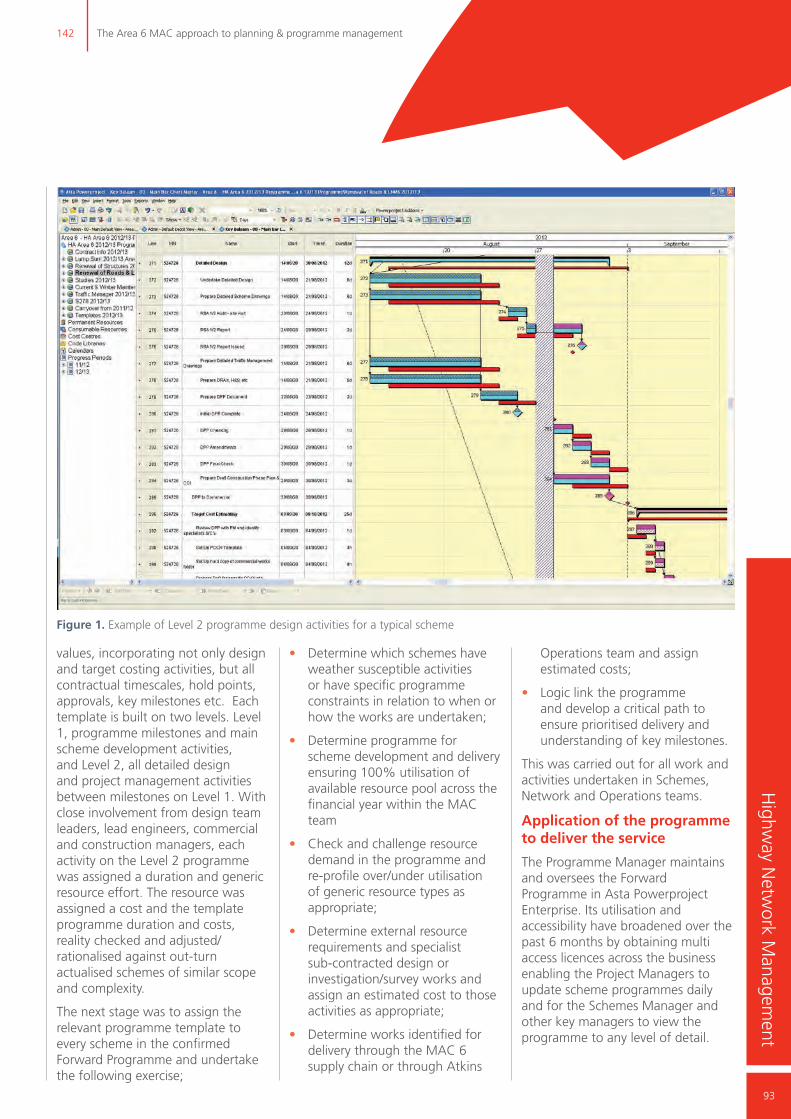
142 The Area 6 MAC approach to planning & programme management
93
Highw
ay Netw
ork Managem
ent
values, incorporating not only design and target costing activities, but all contractual timescales, hold points, approvals, key milestones etc. Each template is built on two levels. Level 1, programme milestones and main scheme development activities, and Level 2, all detailed design and project management activities between milestones on Level 1. With close involvement from design team leaders, lead engineers, commercial and construction managers, each activity on the Level 2 programme was assigned a duration and generic resource effort. The resource was assigned a cost and the template programme duration and costs, reality checked and adjusted/rationalised against out-turn actualised schemes of similar scope and complexity.
The next stage was to assign the relevant programme template to every scheme in the confirmed Forward Programme and undertake the following exercise;
Figure 1. Example of Level 2 programme design activities for a typical scheme
• Determine which schemes have weather susceptible activities or have specific programme constraints in relation to when or how the works are undertaken;
• Determine programme for scheme development and delivery ensuring 100% utilisation of available resource pool across the financial year within the MAC team
• Check and challenge resource demand in the programme and re-profile over/under utilisation of generic resource types as appropriate;
• Determine external resource requirements and specialist sub-contracted design or investigation/survey works and assign an estimated cost to those activities as appropriate;
• Determine works identified for delivery through the MAC 6 supply chain or through Atkins
Operations team and assign estimated costs;
• Logic link the programme and develop a critical path to ensure prioritised delivery and understanding of key milestones.
This was carried out for all work and activities undertaken in Schemes, Network and Operations teams.
Application of the programme to deliver the service
The Programme Manager maintains and oversees the Forward Programme in Asta Powerproject Enterprise. Its utilisation and accessibility have broadened over the past 6 months by obtaining multi access licences across the business enabling the Project Managers to update scheme programmes daily and for the Schemes Manager and other key managers to view the programme to any level of detail.
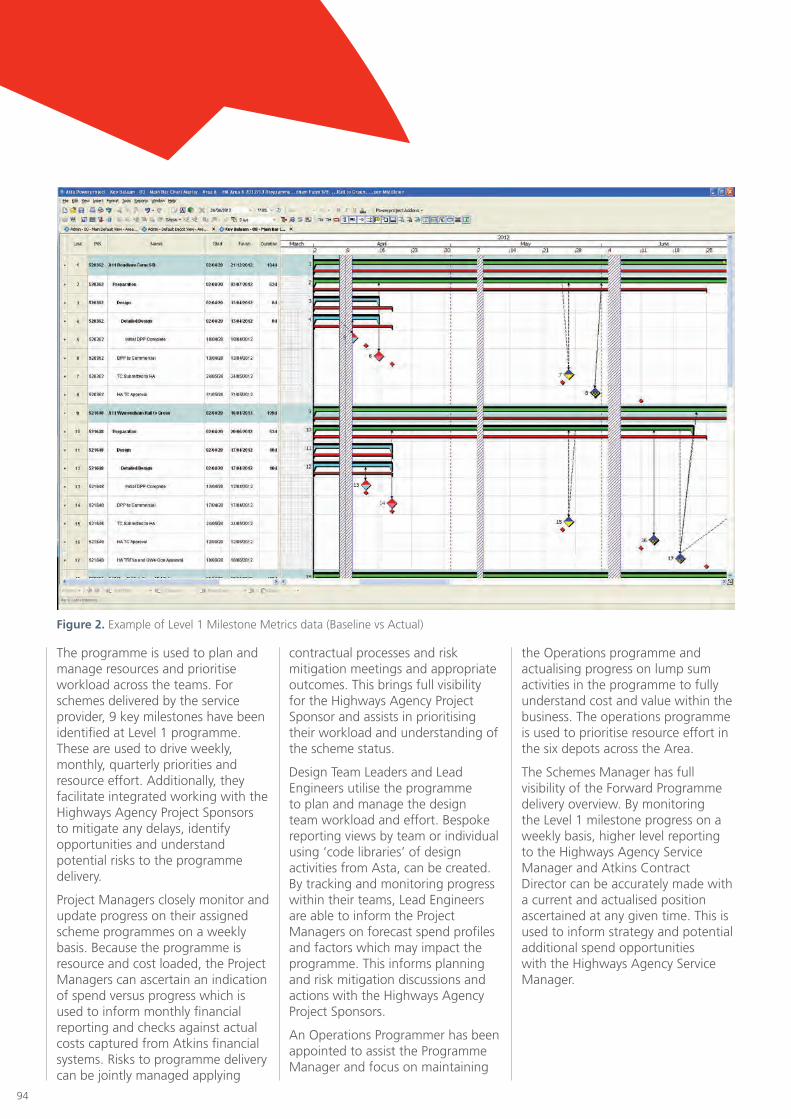
94
The programme is used to plan and manage resources and prioritise workload across the teams. For schemes delivered by the service provider, 9 key milestones have been identified at Level 1 programme. These are used to drive weekly, monthly, quarterly priorities and resource effort. Additionally, they facilitate integrated working with the Highways Agency Project Sponsors to mitigate any delays, identify opportunities and understand potential risks to the programme delivery.
Project Managers closely monitor and update progress on their assigned scheme programmes on a weekly basis. Because the programme is resource and cost loaded, the Project Managers can ascertain an indication of spend versus progress which is used to inform monthly financial reporting and checks against actual costs captured from Atkins financial systems. Risks to programme delivery can be jointly managed applying
contractual processes and risk mitigation meetings and appropriate outcomes. This brings full visibility for the Highways Agency Project Sponsor and assists in prioritising their workload and understanding of the scheme status.
Design Team Leaders and Lead Engineers utilise the programme to plan and manage the design team workload and effort. Bespoke reporting views by team or individual using ‘code libraries’ of design activities from Asta, can be created. By tracking and monitoring progress within their teams, Lead Engineers are able to inform the Project Managers on forecast spend profiles and factors which may impact the programme. This informs planning and risk mitigation discussions and actions with the Highways Agency Project Sponsors.
An Operations Programmer has been appointed to assist the Programme Manager and focus on maintaining
Figure 2. Example of Level 1 Milestone Metrics data (Baseline vs Actual)
the Operations programme and actualising progress on lump sum activities in the programme to fully understand cost and value within the business. The operations programme is used to prioritise resource effort in the six depots across the Area.
The Schemes Manager has full visibility of the Forward Programme delivery overview. By monitoring the Level 1 milestone progress on a weekly basis, higher level reporting to the Highways Agency Service Manager and Atkins Contract Director can be accurately made with a current and actualised position ascertained at any given time. This is used to inform strategy and potential additional spend opportunities with the Highways Agency Service Manager.

142 The Area 6 MAC approach to planning & programme management
95
Highw
ay Netw
ork Managem
ent
and plan team priorities, targets and issues. This is fed back through the Design Team Leaders and relevant Project managers
• Operations team develop visual management from the programme in each of the six depots to enable the Depot Agents to improve forward planning and help facilitate discussions and engagement with the operatives on the Lump Sum activities programme.
Training and support
The Programme Manager was key to developing the Asta Powerproject Enterprise planning and programming solution. Technical support and training were engaged from Asta plc to increase and accelerate knowledge of the software and its potential for broader application across the business. As the MAC 6 expert user and local champion, the Programme Manager produced a User Guide for Project
• Construction team planning and programming boards for mobilisation and construction activities which are used to plan supervision resource deployment, efficient utilisation of the supply chain eg, linking up schemes in the surfacing programme to minimise demobilisation of blacktop gangs and plant;
• Commercial team target cost tracker which is used to manage the milestones within the process for preparing, submitting and approving target cost estimates for Provider Works. It is also used by the Managing QS to balance workload within the QS team, facilitate meetings and progress discussions with the Project Managers and set weekly and monthly priorities
• The roads and structures design teams develop a common visual management tracker to facilitate weekly team meetings to discuss
Developing visual management from the programme
When fully built and populated, Asta Powerproject Enterprise can be utilised to produce bespoke reports at any level of detail built into the programme. The Schemes Manager developed a planning and progress visual management area which is updated daily and is used to monitor the high level priority and actions required to deliver the programme. The Programme Manager produces quarterly, monthly and weekly reports from Asta and updates the visual management boards appropriately. The Schemes manager utilises the boards in discussion and meeting with senior managers and Project Managers in planning and managing the portfolio in a proactive way.
Visual management has broadened across the team driven by the Asta programme to include:
Figure 3. Example of Design Team view (Top Level Summary showing concurrent progression of schemes)

96
Figure 4. Example of Operational Depot programme view (Ardliegh Depot)
Managers and rolled out a series of 1-2-1 on the job training sessions. As experience and competency grew, training was gradually widened across the team and resilience added by creating an Assistant Project Manager post with responsibilities which included an overview role for assisting the Project Management team to ensure the Provider Programme was always up to date on Asta. The most competent IT literate junior staff were encouraged to learn Asta and assist in updating and understanding the programme and functionality.
A Programme driven culture
A key part of the Senior Management Team change management strategy, was to create an environment and culture of programme ownership and delivery. By identifying and implementing the right structure, right tools, right people in key roles, and changing the office layout to encourage
communication, the environment was created.
To develop the culture it was necessary to include every member of the team from trainee technician to Schemes and Commercial Manager in ensuring they understood their contribution to delivering the Providers Programme for the Highways Agency and the importance of taking full ownership for the role and work they undertake. The Schemes Manager undertook workshops with the wider team, key managers and individuals to embed the strategic change of approach and help individuals understand the changes in roles and responsibilities. Wide engagement in building the Annual Plan was encouraged and facilitated to create ownership and understanding. Visual management serves not only to plan and prioritise within the teams, but to create a culture of meeting targets that are openly agreed and monitored.
Benefits to the Highways Agency
The development of the planning and programme approach by the Atkins MAC 6 team has delivered multiple benefits for the Highways Agency:
• Contractual compliance: through visibility on the detailed programme both parties have a clearer understanding of contractual timescales, application of the contract in respect of change control and risk management;
• Highways Agency Project Sponsors are far more involved throughout scheme development and have developed and matured their understanding of the end to end process through monthly progress discussion and ad hoc ‘business as usual’ meetings centred around the programme and activities;

142 The Area 6 MAC approach to planning & programme management
97
Highw
ay Netw
ork Managem
ent
Figure 5. Example of HA Project Sponsor - outstanding key tasks view/report
Figure 6. Stakeholder view- Example of forward works programme within county of Suffolk for Suffolk CC
• Area Performance Indicators (API): time and cost predictability targets have all been ‘green’ for 18 months;
• Highways Agency Performance Management Framework (PMFv8) for MAC and ASC contract – all aspects for measuring performance on delivery of Forward Programme have been ‘green’ for 12 months;
• Cost savings and efficiencies in road space utilisation by identifying opportunities for combining traffic management into single sites or programmes and reducing target cost for individual schemes;
• Potential for the Highways Agency to re-invest efficiency savings into the network;
• Key information for stakeholders quickly produced from Asta
• Efficiency savings on cost reimbursable activities by
combining common design tasks, meetings, site visits etc, across schemes being developed concurrently within the design teams
• Increased confidence in Atkins’ ability to plan, manage and deliver the Forward Programme and Lump Sum activities
• Better working relationships between Atkins and the Highways Agency Area team centred on an agreed Annual Plan and Provider Programme with a desire to work collaboratively and in an integrated manner to jointly deliver.

98
• Early preparation of weather susceptible schemes enables more efficient and risk mitigated delivery.
Continuous improvement initiatives
The following is currently being undertaken or is planned for in the current financial year:
• Quarterly detailed analysis of key programme milestones (forecast versus actual) to assess outturn performance at key scheme development and delivery stages and where improvements and effort should be focussed;
• Building the draft Annual Plan framework for 2013/14 by reviewing resources and programme templates against outturn costs and duration;
• Adopting the same planning and programming approach from the start of the Atkins/Skanska JV ASC Area 2 contract with potential to implement across other Local Authority commissions and Atkins Operational Services contracts;
• Developing visual management initiatives across the business following the Schemes team approach and sharing across
Powerproject Enterprise is recognised as best practice in the MAC/ASC community.
Application of LEAN principles and identification of efficiencies include:
• Single source of monitoring the entire Providers Programme with functionality to bespoke reporting to any level of detail in a simple and quick operation;
• Creation of report templates from the programme to generate monthly data for incorporation into PMF, API, Monthly Business Report and quarterly Business Reporting which reduces duplication and time consuming data analysis;
• Identification of concurrent working potential and efficiency saving on design activities such as combined site inspection, TRIPS meetings, TTRO applications etc. It is estimated that there could be 15% efficiency saving to the client of cost reimbursable design activities during the current financial year;
• Forward planning resource utilisation to maximise productivity and work closely with the Highways Agency Area team to take advantage of potential for early preparation of schemes;
The benefits to Atkins
For Atkins many of the benefits are common in respect of strong consistent performance measures, improved working relationships etc. Other benefits include:
• Clearer visibility to plan and manage resources effectively;
• Confidence in quarterly business reporting to the board of directors and ability to deliver business targets;
• Improved financial forecasting accuracy and checks on actualised costs;
• Improved performance and client feedback in respect of financial reporting;
• Improved commercial performance by maximising revenue potential through being in a position to discuss, prepare early designs or deliver additional work for the Highways Agency;
• Ability to benchmark performance across the key milestones by parts of the business, teams, individuals and discuss improvement plans and adjustments to timescales etc;
• Significant increase in staff morale, motivation and general feeling of being far more in control of the programme at all times;
• Individuals understand their role and how they contribute to delivering the service and business targets.
Innovations and LEAN
The programming and planning solution implemented in MAC 6 is an innovation over the conventional programming approach and has been expanded to include every activity undertaken in delivering the service for the Highways Agency. The level of detail and development built into the Providers Programme using Asta
Figure 7. 2012/13 Q1 review showing average variance to baseline Annual Plan (working days) at key Level 1 programme milestones

142 The Area 6 MAC approach to planning & programme management
99
Highw
ay Netw
ork Managem
ent
Operational Services with an initial focus in Area 2 ASC
• Capturing outturn performance data for programme and costs and feeding into the 2013/14 Continuous value management process and bid submission to increase accuracy and confidence in budget allocations at funding.

100

Structural Dynam
ics143
101
Simon Ratcliffe
Engineer
Defence, Aerospace & Communications
Atkins
Determination of minimum vessel wall thickness under design condition loadingsAbstract
During the concept design phase of a series of pressure vessels for nuclear application, an approach was developed to provide minimum vessel sizing under dynamic loading conditions. Calculations had been undertaken to determine an initial tentative vessel wall thickness using ASME III Subsection NB, however only a limited assessment of mechanical loading was undertaken.
This paper outlines a static analysis approach for extending the structural analysis of a pressure vessel shell to include design condition loadings. These include dynamic loading, support reactions and external piping reactions which can have a significant influence on the required minimum wall thickness.
This paper is limited to outlining generic rules and assumptions that can be applied to the preliminary concept design of pressure vessels. The method was originally captured to aid knowledge sharing within the design team. It does not prescribe an exact methodology but rather an interpretation and application of the design code. The aim is to provide a better defined vessel geometry upon which to base the detailed finite element stress analyses for both design and service conditions. The perceived benefit of this approach is that there will be a lower likelihood of major design changes being made during the detailed design phase.
Nomenclature
Pm General primary membrane stress
Pl Local primary membrane stress
Pb Primary bending stress
Sm Allowable stress intensity
S Stress difference
P Internal design pressure
g Acceleration due to gravity
t Tentative pressure thickness
R Internal radius of vessel
∆P Increase in internal pressure
ρ Density
h Height of fluid in the vessel
Wz Vertical acceleration
Fz Force in vertical direction
m Mass of vessel
σ Component stress
σp Principal stress

102
condition loadings. Secondary stresses in the shell and stresses in the mounting features and vessel attachments themselves are not considered as part of this work.
Assumptions
The assumptions stated below are considered common to most cylindrical vessels and relevant to the approach described in this paper. Additional specific assumptions for individual vessels may be required when the methods outlined here are put into practice:
a) The vessel is assumed to be full of the working fluid – this removes the effects of ‘sloshing’ fluid within the vessel;
b) The vessel centre of gravity is at its geometric centre;
c) The vessel is cylindrical and features spherical heads;
d) The vessel length is much greater than the radius;
e) Dynamic loading input can be interpreted as an equivalent static load acting at the vessel centre of gravity expressed in terms of gravitational acceleration (g);
f) Vertical (z axis) and horizontal (x and y axes) dynamic loadings are considered to be acting independently of each other and in isolation;
g) The vessel can be assumed to be symmetrical about the vertical axis and the greater of the two horizontal dynamic loads (x and y axes) will be used as the bounding load case alongside the vertical dynamic load;
h) The total stress at each location will be assessed by summing the contributions from each loading condition irrespective of its sign. This is a conservative assumption and may be open to review should it result in
Scope
The methods for calculation outlined here assume that the vessel is classified as Class 1 and assessed against stress intensity limits in the American Society of Mechanical Engineers Boiler and Pressure Vessel Design Code Section 3 (ASME III) Division 1 Subsection NB1. The vessel is cylindrical in shape and contains a working fluid (See Figure 1). It is a prerequisite that analyses to determine the dynamic response of the pressure vessel on its support structure have been undertaken in order to determine the actual equipment acceleration that is to be used in the structural analysis.
The calculation uses a static analysis based on the load cases in Roark’s Formulas for Stress and Strain2 and is intended to be conservative by nature. Local stresses in the shell associated with nozzles and the mounting features are to be calculated in accordance with methods contained in Annex G of PD 5500-20093. Alternative open literature calculation methods shall be used if the mounting geometry is not suitable to be modelled using References 2 and 3.
This report is limited to outlining generic rules and assumptions that can be applied to ASME Class 1 vessels for calculating minimum thickness requirements. It does not prescribe an exact methodology for specific vessels but rather a general approach. The guidance given here is intended to be used to assist in the hand calculation and assessment of stresses and minimum wall thicknesses due to design condition loadings.
Only general primary membrane, primary bending and local primary membrane stresses in the shell of the vessel will be included in the assessment. Compliance with primary stress limits ensures that the wall thicknesses are adequate to prevent gross yielding under design
Introduction
ASME III NB rules for tentative pressure thickness and reinforcement requirements for openings enable only a very limited initial vessel sizing to be undertaken. This assessment is based on design pressure and design temperature alone. Design mechanical loads, such as those resulting from shock or seismic effects also require a preliminary assessment. These dynamic loadings can have a significant influence on the required minimum wall thickness.
This paper describes a methodology for determining the minimum wall thickness requirement for pressure vessels subject to high external dynamic loading. Such loading can arise potentially on pressure vessels used in nuclear plant, the offshore industry and in some military applications due to earthquake, blast and external impact.
The methodology extends the structural analysis of ASME Class 1 pressure vessels to include all design condition loadings comprising the combination of design pressure and temperature, dynamic loading, support reactions and external piping reactions on nozzles. The approach uses well documented hand calculation techniques to determine minimum wall thicknesses and nozzle reinforcement requirements.
The aim of this approach is to provide an improved defined vessel geometry upon which to base the detailed finite element stress analyses for both design and service condition loadings at the detailed design phase. The perceived benefit of the approach described in this paper is that there will be a much lower likelihood of major design changes being required to be made to the vessel during the detail phase, which if they occur can have adverse cost and timescale implications on the project.

143 Determination of minimum vessel wall thickness under design condition loadings
103
Structural Dynam
ics
excessively large wall thicknesses;
i) The allowable stress intensity (Sm) is evaluated at the design temperature of the vessel.
General approach
The approach described in this paper is intended to provide basic pressure vessel sizing and optimisation prior to undertaking a detailed stress substantiation of the vessel. The general approach is based on calculating a tentative thickness for the vessel shell under design pressure and temperature conditions. This is then assessed to establish whether an increase in thickness is required from consideration of all design condition loadings.
This paper focuses on dynamic loading resulting from shock, vessel support reactions and pipe loads on the vessel shell as the key design mechanical loadings.
The following regions on the vessel and corresponding load cases are considered for assessment as part of this methodology.
Calculation sequence
The outline of the approach described in this paper assumes that calculations are undertaken in the following sequence:
• calculation of tentative pressure thickness for main shell and heads in line with ASME III NB-33241
• assessment of stresses in shell and heads under design pressure loading against ASME III criteria
• calculation of stresses in main shell and head remote from discontinuities under dynamic loading
• calculation of stresses in vessel wall adjacent to nozzles and mounting features under dynamic loading
• calculation of principal stresses for each load case
• calculation of stress intensities
• calculation of reserve factors
Table 1. Summary of vessel regions being considered and the applicable load cases
Table 2. Limits of stress intensity from ASME III Figure NB-3221-1 and NB-3227.2
• repeat calculation if necessary with an increased wall thickness until the required reserve factor is achieved.
Stress Categorisation and Allowable Stress Intensity
Principal stresses are required to be calculated for the assessment of design condition loadings. These consist of General Primary Membrane (Pm), Local Primary Membrane (Pl) and Primary Bending (Pb) stress categories. Figure NB-3221-1 in ASME III [1] shows the allowable limits of stress intensity for Class 1 vessels and is summarised in Table 2.
As stated in NB-3221.3 of ASME III1, the allowable value of primary membrane (general or local) plus primary bending stress intensity is Sm multiplied by a shape factor, which for a solid rectangular section is 1.5 (See Table 2). NB-3221.3 should be referred to for other geometries. It should be noted that the shape
Figure 1. Sketch Of Generic Cylindrical Vessel
Vessel Part/Region Load Case
Vessel shell (remote from discontinuities)
Internal pressure plus dynamic loading
Vessel heads (remote from discontinuities)
Internal pressure plus dynamic loading
Vessel shell local to nozzles Internal pressure plus dynamic loading plus external loading from pipe work
Vessel shell local to mounting pointsInternal pressure plus dynamic loading plus external loading from pipe work
Stress CategoryMaximum Allowable Stress Intensity
Pm Sm
Pl 1.5 Sm
Pm + Pb 1.5 SmPI + Pb
Pure Shear
0.6Sm average primary shear stress across section
0.8Sm maximum primary shear stress across section in torsion

104
factor shall not exceed the value calculated for bending only and in no case shall it exceed 1.5.
Assessment of stress intensity
In order to assess the vessel shell thickness for suitability under design condition loading, it must be established whether the stress intensity in the shell exceeds the specified limits. These limits differ depending on the category of stress present in the shell (see Table 2). The following sections describe the process by which the stress intensity is calculated and then compared with the allowable limits. This procedure is described in ASME III NB-3215.
Principal Stresses
At the location on the vessel being investigated, an orthogonal set of coordinate axes should be selected. For many pressure vessels it is possible for these axes to be chosen such that the shear stress component is zero. This helps to simplify the calculation of principal stresses. For cylindrical vessels, orthogonal axes in the radial, tangential and longitudinal direction are recommended.
At each location calculate the stress components in each axial direction for each load case. These stresses are then assigned an appropriate category in line with the guidance set out in ASME III Table NB-3217-1. The algebraic sum of the stresses in each category should then be found. As specified in NB-32151, the sum of the stresses in the general primary membrane stress, local primary membrane stress, general primary membrane stress plus bending stress and local primary membrane stress plus bending stress are all assessed separately for each load case. These stresses are then translated into principal stresses as described in Roark’s Formulas for Stress and Strain2. For thick walled vessels where the axes have been selected such that there is no shear
component, the calculated stresses in each direction translate directly into three principal stresses. Under the assumption that the shell is thin walled, the radial stress component is negligble, the remaining two are calculated as follows;
Equation 1
Equation 2 Table 2.3, Reference 2
The principal stress σp3 is therefore zero for the purposes of calculating the stress differences S12, S23 and S31.
Stress Intensity
From ASME NB-3215(e)1 the stress differences are then calculated as follows:
Equation 3
Equation 4
Equation 5
The stress intensity is the largest absolute value of the stress differences calculated above which can then be compared to the allowable stress intensities listed in Table 2.
Reserve factors
Assessment of the stress intensity is achieved by calculating reserve factors. The reserve factor is equal to the allowable stress intensity divided by the calculated stress intensity. Generally, a reserve factor of unity or greater indicates that the vessel wall thickness and area reinforcements local to openings are adequate for the design condition loadings.
Where reserve factors are found to be less than unity, it may be due to conservatism in the assumptions and methods used to calculate the stress intensities. Where appropriate, assumptions and methods should be refined to remove pessimism and the reserve factors recalculated.
If it is deemed that the treatment of assumptions is independent from the reserve factors being below unity, then the calculations should be repeated with an increased wall thickness until acceptable reserve factors are achieved.
In the case of assessing initial pressure thickness calculated using NB-3324; where the reserve factor is less than unity the wall thickness should be increased in the first instance.
Appendix 1 outlines an example calculation concerning a simple cylindrical shell subject to internal pressure plus dynamic loading. It demonstrates the initial vessel thickness being increased in order to give an acceptable reserve factor under dynamic loading.
Tentative pressure thicknesses and opening reinforcement
Initial Design Pressure Thickness
An initial value for vessel wall thickness can be calculated using the formulae given in ASME III NB-3324.
Equation 6
Where:
t = Tentative pressure thickness
P = Internal design pressure
R = Internal radius of vessel
Sm = Allowable stress intensity for the material
σp1 =12
(σx + σy) + (σx - σy)2 + 4.t
xy2
σp2 =12
(σx + σy) + (σx - σy)2 + 4.t
xy2
S12 = σp1 - σp2
S23 = σp2 - σp3
S31 = σp3 - σp1
t = P.RSm - 0.5P

143 Determination of minimum vessel wall thickness under design condition loadings
105
Structural Dynam
ics
This formula is based on the assumption that the vessel is thin walled.
Initially, the thickness of the vessel heads is assumed to be equal to that of the main cylinder wall. The primary stresses in the vessel shell due to design pressure and temperature loading can then be calculated and assessed against the relevant design criteria.
Nozzle and Opening Area Reinforcement
Nozzles and openings in the shell require a minimum level of local material reinforcement which should be considered when calculating the minimum pressure thickness of the shell. The calculation of this reinforcement is based on design pressure and temperature loading and supplements the minimum pressure thickness. ASME III NB-3332 gives rules for the calculation of nozzle reinforcement based on design pressure loading. This can then be assessed against dynamic loading from pipe work.
Preliminary stress assessment of design condition load cases
Assessment of Static Pressure Load
Once an initial pressure thickness has been calculated for the vessel it requires assessment to ensure that it can withstand the design condition pressure loading. The following paragraphs describe the general membrane stresses that are present in the shell under such loading.
Main Cylindrical Body
The main body of the vessel shell is considered separately from the vessel heads and is a cylinder with capped ends. The axial and hoop primary membrane stresses in the shell under uniform internal or external pressure, can be calculated using Case 1c in Table 13.1 from Roark’s Formulas2.
The radial stresses are assumed to be negligible in comparison with hoop and axial stresses.
Vessel Heads
Primary membrane stresses will also be present in the upper and lower heads of the vessel. These are calculated using the appropriate load case based on the geometry of the head. This paper only considers spherical and torispherical head geometries common on many pressure vessels. There is not the scope to consider more complicated geometries. For a spherical head under uniform internal pressure, Roark’s gives formulae for the meridional and tangential stressCase 3a,
Table 13.1, Reference 2. The crown region of a torispherical head can be assessed using the same formulae.
Discontinuity stresses resulting from the changes in section between the shell and the head are not assessed in this calculation neither is the knuckle region of a torispherical head.
Assessment of Shell Thickness under Mechanical Design Condition Loadings
Once the minimum shell pressure thickness has been established, further hand calculations can be undertaken to assess this thickness for suitability under other design condition loading. The loads considered by this paper are vertical dynamic loading, horizontal dynamic loading, local loads applied to the vessel shell by mounting features and pipe work reactions.
The following section contains guidance for approximating these load cases and calculating the resulting stresses in the shell. These stresses are then categorised and assessed against the design criteria outlined in Table 2. The aim of the assessment is to provide sufficient margin in the vessel thickness to withstand mechanical loadings before the design is progressed to the detailed design phase.
Vertical Dynamic Loading
For vertical dynamic loading it will be assumed that the vessel is accelerated upwards. The resulting downwards force will therefore be equal to the mass of the vessel and contents multiplied by the acceleration.
Equation 7
Where the upper and lower head of the vessel have different geometries, rather than considering an upwards and downwards acceleration, the same dynamic loading will be applied to both heads.
Axial Stress in Shell
The cylindrical shell will see an increase in axial load due to the increase in effective weight of the fluid in the vessel and similarly due to the increase in effective weight of the vessel material.
Mass of Fluid
When the vessel is accelerated upwards, the mass of the fluid is effectively acting downwards within the vessel. This will generate an axial stress in the vessel shell equal to the downwards force of the fluid under acceleration divided by the vessel shell cross sectional area. In order to ensure a conservative outcome, the total mass of the fluid will be used and the stress analysed at the thinnest section of the vessel shell.
Mass of Material
The vessel shell loaded by its own weight will experience an axial membrane stress. When the vessel is accelerated upwards, the effective weight of the vessel material will increase resulting in additional axial membrane stress. This load case is the same as that outlined in Case 1e of Table 13.1 in Roark’s Formulas2. The axial stress is calculated by multiplying the force per unit volume of the material by the total height of the cylindrical shell, where the force per unit volume is equal to the density of the vessel material
FZ = m.(WZ)

106
multiplied by the acceleration. The increase in load caused by acceleration of the lower head is also included in the calculation. In order to ensure a conservative calculation, the compressive stress in the shell above the upper mounting position caused by acceleration of the upper head is neglected.
Hoop Stress in the Shell
The vertical acceleration of the vessel will also result in an increase in hoop stresses in the shell due to the increase in the effective weight of the fluid. This is calculated based on the total mass of fluid in the vessel. In order to calculate the hoop stress in the shell, the increase in effective fluid weight is treated as an increase in internal pressure in the vessel. This allows internal pressure load cases to be used to calculate the hoop stress.
The hoop stresses in the shell as a result of internal pressure loading are found using Case 1c in Table 13.1 from Roark’s Formulas2. In this case however, the pressure is calculated from the head of fluid above the lowest point in the vessel with acceleration due to gravity replaced by the acceleration.
Equation 8
Stresses in the Head
The lower head will see an increase in axial (meridional) and hoop stresses due to the increase in effective weight of the fluid in the vessel and similarly due to the increase in effective weight of the vessel material.
Mass of Fluid
The vertical acceleration of the vessel will result in an increase in the stresses in the lower head due to the increase in the effective weight of the fluid. Again as with the stresses in the vessel shell, this is calculated based on the entire mass of fluid and is treated as an increase in internal pressure load acting on the head.
The stresses resulting from the increase in the effective weight of the fluid will be calculated using Case 3a, Table 13.1 from Roark’s Formulas for Stress and Strain2; however, the hydrostatic pressure will be replaced by the design pressure plus that under acceleration as shown in Equation 8.
If the lower and upper heads have different geometries, then the stresses in both heads shall be analysed, assuming the most conservative loading on each.
Mass of Material
The vessel head loaded by its own weight will generate membrane stresses. In this case both meridional and hoop stress will occur. The acceleration will cause the effective weight of the material in the vessel head to increase and the resulting force per unit volume shall be calculated by multiplying the density of the material by the acceleration. The stresses are calculated in line with the Case 3c given Roark’s Formulas Table 13.12.
Horizontal Dynamic Loading
Where the horizontal acceleration has been split into two planes (e.g. x and y) the greater of the two accelerations should be used when calculating the horizontal dynamic loading. This approach relies on the assumption that the vessel can be considered symmetrical about the vertical axis.
Bending Stress in the Shell due to Direct Loading
Depending on the way the vessel is mounted, axial and hoop bending stresses will be generated in the vessel shell under horizontal dynamic loading. The method of calculation of these bending stresses uses an approximation of the vessel as an elastic beam under bending. Different beam approximations can be used to most closely represent the way the vessel is mounted. For example, in the case of two
mounts at opposite ends of the vessel, a simply supported beam approximation may be appropriate.
To ensure a conservative calculation, the entire mass of the vessel, including contents, is treated as a uniformly distributed load applied along the length of the vessel. The maximum bending moment can then be calculated and the simple theory of bending used to find the maximum axial bending stress. This stress is categorised as a membrane stress, rather than bending stress, due to the very small stress gradient created through the wall. See Table NB-3217-1, ASME III1.
Average Shear Stress in the Shell
Treating the vessel as an elastic beam, the average shear force can be found by dividing the total load on the vessel by the number of supports assumed under the beam approximation.
The average shear stress in a hollow cylindrical beam or shell is calculated by dividing the shear force by the cross sectional area of the shell and assessed against 0.6Sm in accordance with ASME NB-3227.2(a)1.
Hoop Membrane Stress in the Shell and the Vessel Heads due to Increase in Effective Weight of Fluid
The method used in the vertical loading case for evaluating increased pressure stresses in the shell due to the increase in effective weight of the fluid contents is unsuitable for the horizontal loading. This is due to the pressure not being uniform across the vessel diameter which will generate distortion and bending stresses.
However the vertical loading case considered here involves a much greater height of fluid than the vessel internal radius and so is assumed to provide sufficient margin on the vessel thickness. Horizontal pressure stresses should therefore
∆P = ρ.h.(Wz)

143 Determination of minimum vessel wall thickness under design condition loadings
107
Structural Dynam
ics
be accounted for by applying the increase in pressure under vertical acceleration to the horizontal load case. This will allow a conservative assessment of the stresses in the shell under horizontal loading to be included.
Calculation of stresses in vessel wall adjacent to nozzles and mounting features
Vessel Wall Adjacent to Nozzles
The applied loads at pipe work attachments to nozzles are often not known at the concept design stage. Therefore the maximum load (end thrust, bending, shear and torsion) that can be applied to the nozzle by the pipe work shall be calculated based on the assumption that the stress in the pipe reaches the maximum value permitted by the ASME design code for pipe work. Details of the approach are provided below.
External Moments Applied to the Vessel Shell
The reaction of pipe work due to expansion and dynamic loading will apply a moment to the vessel shell. This moment shall be calculated assuming a maximum bending stress in the pipe of 1.5Sm. For most cylindrical vessels that are intended to be vertically mounted, the method by which these moments are calculated is shown in Subsection 2.3, Annex G of PD 5500-20093 where vertical dynamic loading translates to a longitudinal moment and horizontal dynamic loading translates to a circumferential moment. These will be analysed using Subsection G.2.3 and suggested working forms G2 and G1 respectively. PD 5500-20093 has been selected in this case because it contains relevant formula for calculating local component stresses. The assessment of these stresses will still be against the criteria
laid out in ASME III Subsection NB1 for consistency.
Radial Loads Applied to the Vessel Shell
Loads on the vessel shell resulting from pipe work are assessed using a limit load analysis. Under horizontal dynamic loading, the reaction of the pipe work is assumed to create a radial load on the vessel shell. This shall be calculated assuming a maximum direct stress in the pipe work of 1.5Sm based on the pipe work material. The load is then the maximum stress in the pipe multiplied by the cross sectional area of the pipe work attachment. The corresponding stresses in the vessel shell are then calculated as outlined in Subsection G.2.2 in Annex G of PD 5500:2009.
Shear due to Pipe Work
The maximum shear load that can be applied to the nozzle by the pipe work shall be calculated based on the ASME limit of 0.6Sm and the known cross sectional dimensions of the pipe work. Note that in this case the allowable stress intensity value, Sm, is that for the pipe work material. Similarly for shear stress as a result of torsion in the pipe work, the maximum torsional moment that can be applied to the nozzle by the pipe work shall be calculated based on the ASME limit of 0.8Sm as defined in NB-3227.2(b) of ASME III1.
Gross Discontinuity Stress Adjacent to Nozzle Opening
Calculation of Discontinuity Stress
Both primary and secondary categories of discontinuity stress exist local to the nozzle opening. For the purposes of this paper however, only those categorised as local primary membrane stresses in accordance with Table NB-3217-11 are considered. In order to assess the total stress in the region adjacent to the nozzle, the gross discontinuity stresses are required in addition to the average membrane stresses resulting from pressure load.
The discontinuity stresses should be calculated in accordance with the methodology outlined in Welding Research Council (WRC) Bulletin 3685.
Assessment of Discontinuity Stress
These stresses are then added to those from external loadings to get the total stresses in the shell and in the nozzle for comparison with the ASME III limits. The inclusion of discontinuity stresses as outlined here is intended to give an indication of the local stresses prior to the undertaking of detailed finite element techniques during the detailed design stage.
Mounting Features
The stresses in the shell resulting from the mounting features under dynamic loading are also required. These stresses shall be calculated based on the local support loadings on the vessel shell. The reaction at the supports due to vessel mass and external pipe reactions contribute to the local support loading. The exact method of assessment will depend on the nature and number of mounts, but generally these loads should be treated as moments applied to the vessel shell and calculated in a similar manner to stresses as a result of pipe work attachments.
The effects of the pipe work reactions at the vessel mounts can be calculated using a moment balance and represent the additional stress at each mounting point as a result of the pipe work attachments under dynamic loading.
The stresses in the shell as a result of the reactions at mounting points shall be calculated using methods contained in Subsection G.2.3 of Annex G of PD 5500:2009 where appropriate. Should the specific mounting features of the vessel not be covered in Annex G, alternative sources of load cases should be sought.

108
The stresses in the shell adjacent to the mounting features as calculated above shall be added to the appropriate hoop or axial stress in the shell due to internal pressure (plus the increase in pressure arising from increased effective mass of fluid due to dynamic loading) to determine the total stress in the shell at the mounting.
Conclusions
This paper has described an approach for extending the structural analysis of ASME Class 1 pressure vessels to include all design condition loadings. These loads comprise the combination of design pressure and temperature, dynamic loading, support reactions and external piping reactions on nozzles. Open literature and hand calculation techniques have been employed to determine minimum wall thicknesses and nozzle reinforcement requirements. Assessment of stress intensities has been in line with the ASME III Subsection NB design criteria.
Appendix 1 demonstrates part of the methodology being applied to a simple cylindrical shell. An initial tentative pressure thickness is calculated and then dynamic loading applied. The calculation shows that in order to generate adequate reserve factors under high dynamic loading, the initial pressure thickness must be increased.
Acknowledgments
This paper was previously published in the proceedings of the ASME Conference, Toronto, July 2012.
The author would like to acknowledge the help and support of Jonathan Edward Pope (Atkins) who has provided technical guidance and mentoring throughout. Recognition should also go to Richard Russell-Johnson (Atkins), Peter Goodman (Atkins), Mark Selden (Atkins) and Sam Arnold (Atkins) for their help with the paper. And finally to Atkins for funding this endeavour.
References
1. ASME, 2010, ASME Boiler & Pressure Vessel Design Code, Section III, Division 1, Subsection NB, American Society of Mechanical Engineers.
2. Young, W.C. and Budynas, R.G, Roark’s Formulas for Stress and Strain, McGraw-Hill, Seventh Edition, 2002.
3. BSI, 2009, PD 5500:2009, Specification for Unfired Fusion Welded Pressure Vessels, British Standards Institution, 2009.
4. ASME, 2010, ASME Boiler & Pressure Vessel Design Code, Section II, American Society of Mechanical Engineers.
5. Mokhtarian, K. And Endicott, J.S, Stresses in Intersecting Cylinders Subjected to Pressure, WRC Bulletin 368, Welding Research Council, November 1991.

143 Determination of minimum vessel wall thickness under design condition loadings
109
Structural Dynam
ics
Appendix A
Example Calculation of Vessel Pressure Thickness and Assessment under Dynamic Loading
The following calculation demonstrates the methodology outlined in the paper. The appendix is limited to assessing the pressure thickness and dynamic loading on a simple cylindrical shell excluding heads purely as a demonstration of the theory. The shell is assumed to be orientated with its longitudinal axis vertical and filled with an incompressible working fluid. The calculation will consider primary membrane stress and primary bending stress only.
Inputs
Vessel internal length
Li = 1500 mm
Vessel internal radius
Ri = 160 mm
Density of working fluid
ρfluid = 996 kg/m3
Design stress intensity of vessel material
Sm = 96 MPa
Density of vessel material
ρsteel = 7800 k/m3
Dynamic acceleration (vertical)
Wv = 25g
Dynamic acceleration (horizontal)
Wh= 30g
Design pressure P = 100 bar
Calculation of Tentative Pressure Thickness
The calculation for the tentative pressure thickness of a cylindrical shell can be found in paragraph NB-3324 of Section NB and calculated as follows:
ttent := 18mm
ttent :=P.R.
i
Sm - 0.5P
Equation 9
To check the acceptability of this result, the stresses generated in a shell of this thickness under both vertical and horizontal dynamic loading are calculated and assessed against the stress acceptance criteria in ASME III.
Assessment under Vertical Dynamic Loading
Using the tentative thickness calculated above, the shell has the following physical values:
Equation 10
Shell outer radius
Equation 11
Total mass of the shell and fluid
Under vertical dynamic loading the effective weight of the entire mass of the vessel and contents is increased. This is modelled as a downward force acting on the vessel and will generate axial membrane stress in the vessel shell.
Equation 12
Axial membrane stress in the shell due to vertical dynamic load
The vertical acceleration of the vessel also results in an increase in the membrane stresses in the shell due to an increase in effective weight of the working fluid within. This is modelled as an increase in internal pressure
Ro :=Ri + tshell
Ro = 178mm
mtotal := (Ro2 - Ri
2) π Li ρsteel + Ri2 π Li ρfluid
mtotal = 344kg
σa.v = 4.41 MPa
σa.v := mtotal Wv
π (RO2 -Ri
2)
and allows internal load cases to be used to calculate the hoop stress. The increase in pressure is calculated by multiplying the density of the fluid, by the height of the fluid inside the vessel and then by the dynamic acceleration.
Equation 13
Increase in internal pressure under vertical dynamic loading
∆P := ρfluid Li Wv
Equation 14
Total increased internal pressure due to dynamic loading
Pv.shock := P + ∆P The vessel is considered to be thick walled and therefore Case 1b, Table 13.5 on page 683 of Roark’s Formulas for Stress and Strain is used to calculate the pressure stresses at any chosen radius, r. In this case, the internal pressure is equal to the design pressure plus the increase in internal pressure under vertical dynamic load calculated above.
Equation 15
Axial membrane stress due to internal pressure
Equation 16
Hoop membrane stress due to internal pressure
Equation 17
Radial membrane stress due to internal pressure
The membrane stresses at both the inner and outer radius are calculated using equations 14 to 16 and the mean average taken.
σam =Pv.shock Ri
2
Ro2 - Ri
2
σhm =Pv.shock Ri
2(Ro2 + r2)
r2(Ro2 - Ri
2)
σrm =-Pv.shock Ri
2(Ro2 + -r2)
r2(Ro2 - Ri
2)

110
Equation 26
Maximum bending moment
Equation 27
Second moment of area for a cylindrical section
Equation 28
Distance from neutral axis
Equation 29
Resulting maximum bending stress
σb.shell = -11.708 MPa
Under horizontal load the increase in effective weight of the fluid will again be modelled as an increase in internal pressure and therefore induce membrane stresses in the shell. Since the length of the vessel is significantly greater than the diameter, the increase in vessel internal pressure estimated under the vertical load case is considered to provide sufficient margin on the vessel thickness and can be applied under horizontal dynamic loading.
The shell stresses resulting from horizontal loading are then used to calculate the principal stresses in the shell. The axial bending stress across the entire section of the vessel is considered to be a primary membrane stress in accordance with ASME III Table NB-3217-1 and so is added to the axial membrane stress as a result of internal pressure.
Stress intensity
Sv = 97.604 MPa
The reserve factor is then calculated against Sm.
Equation 24
Reserve factor
The reserve factor calculated is less than 1 which indicates that the shell pressure thickness will not withstand vertical dynamic loading conditions and will need to be increased.
Assessment under Horizontal Dynamic Loading
Under horizontal dynamic loading the vessel shell will see a force acting on it equivalent to the mass of the vessel shell and its contents under horizontal dynamic loading acceleration. This force will be treated as a uniformly distributed load acting over the length of the vessel. The shell is modelled as a beam of hollow cylindrical cross section, simply supported by a single support at both ends. This load will give rise to a bending moment in the shell and hence an axial bending stress. An average shear force across the shell will also be present. This will be assessed separately.
Equation 25
The total force per unit length of vessel
The maximum bending moment will occur at the centre of the length of the vessel. The distance to the neutral axis is taken as the mean radius. This calculates the average stress in the wall at the section of maximum bending moment.
Mean axial membrane stress
σam.v = 43.619 MPa
Mean hoop membrane stress
σhm.v = 92.421 MPa
Mean radial membrane stress
σrm.v = -5.183 MPa
The membrane stresses in each plane resulting from vertical dynamic loading are summed before calculation of the principal stresses.
Equation 18
Axial membrane stresses
σm.v1 := (σam.v + σa.v)
Equation 19
Hoop membrane stresses
σm.v2 := σhm.v
Equation 20
Radial membrane stresses
σm.v3 := σrm.v
The axes have been chosen such that the three principal stresses are taken to equal the stresses calculated above. The stress differences and stress intensity can then be calculated in accordance with paragraph NB-3215 in ASME III.
Equation 21
Stress differences
Sv12 := σm.v1 - σm.v2
Sv12 = 44.392 MPa
Equation 22
Sv23 := σm.v2 - σm.v3
Sv23 = 97.604 MPa
Equation 23
Sv31 := σm.v3 - σm.v1
Sv31 = -53.212 MPa
The stress intensity is equal to the stress difference of greatest magnitude.
RFv := = 0.98SmSv
Fshell.h :=mtotal
.Wh
Li
Mbend :=-Fshell.h Li
2
8
I := π(Ro
4 - Ri4)
4
y:= Ro - Ri
2
σb.shell:= Mbend
.y
I

143 Determination of minimum vessel wall thickness under design condition loadings
111
Structural Dynam
ics
Membrane stress under horizontal dynamic loading
RFh = 1.09
Average shear stress under horizontal loading
RFshear.h = 22.6
Equation 35
Shell shear area
Ashell.shear := π (R02 - Ri
2)
Equation 36
Average shear stress in the shell
tshell = 2.646 MPa
The average shear stress in the shell is assessed by comparing it to the allowable stress intensity for pure shear as defined in ASME III Section NB-3227-2.
Equation 37
Reserve factor for average shear
Increased Shell Thickness
In order to provide confidence that the shell is able to withstand dynamic loading conditions, the vessel wall thickness is increased until the reserve factors under both vertical and horizontal dynamic loading are greater than 1. The results in this case are shown below.
Updated shell thickness to account for dynamic loading
tshell.new := 20mm
Repeating the calculations using the new shell thickness gives the following results for reserve factor. This demonstrates that the increased shell thickness now provides sufficient margin to withstand design condition dynamic loading in both vertical and horizontal directions.
Membrane stress under vertical dynamic loading
RFv = 1.09
Equation 30
Principal stresses
σm.h1 := σb.shell + σam.h
Equation 31
σm.h2 := σhm.h
Equation 32
σm.h3 := σrm.h
The stress differences and stress intensity can then be calculated as shown previously. The reserve factor is then found.
Stress intensity under horizontal dynamic loading
Sh = 97.604 MPa
Equation 33
Reserve factor
The reserve factor calculated is less than 1. This indicates that the shell pressure thickness will not withstand horizontal dynamic loading conditions and should be increased.
Assessment of Average Shear
The shear stress acting in the beam due to bending is assessed separately. In general the average shear stress is significantly smaller than the membrane stresses but has been assessed to provide a more thorough assessment. Using general beam bending theory the shear force acting on the beam is calculated by dividing the total load on the vessel by the number of supports; in this case assumed to be two. The average shear stress is calculated by dividing the shear force by the cross sectional area on which the shear force acts.
Equation 34
Shear force in the shell
RFh:= = 0.98SmSh
Qshell:=mtotal
.Wh
2
tshell :=Qshell
Ashell.shear
RFshear.h := = 21.770.6 Smtshell

112

Jan Winkler
Structural Engineer
Atkins Denmark
Atkins
Jesper Schaarup
Regional Head of Bridge Engineering
Atkins Denmark
Atkins
Structural Dynam
ics144
113
IntroductionIncreasing bridge stock numbers and a push for longer cable-supported span lengths have led to an increased number of reported incidents of damage and replacement of bridge stay cables due to wind and traffic-induced fatigue and corrosion (Winkler & Georgakis 2011). Limited work has been undertaken to assess thoroughly the fatigue characteristics of bridge cables subjected to cyclic transverse deformations as the cables are in principle not expected to experience bending. Furthermore, the commonly applied qualification tests for the fatigue resistance of stay cables (fib 2005, PTI 2007) do not specifically address fatigue issues related to trans-verse cable vibrations and therefore do not require testing for bending. However, recent bending fatigue tests on grouted and PE coated monostrands have shown that monostrands can experience fatigue failure due to high localised deformations (Winkler et al. 2011) and fretting (Wood & Frank 2010).
Cable fatigue failure criteria
The purpose of failure criteria is to predict or estimate the failure/yield of structural members. Although a considerable number of theories
describing the failure criteria for multilayered strands have been proposed (Hobbs & Smith 1983, Hobbs & Raoof 1996), none of these can be applied to monostrands composed of one layer of wires. As the majority of modern stay cables comprise a number of individual high-strength steel monostrands, the understanding of the bending characteristics and failure mechanism of the individual monostrand has become more relevant. It has been reported that the methods seeking to evaluate the fatigue life of the cable should be further developed to be consistent with observed fatigue failures of cables subjected to transverse deformations (Jensen et al. 2007, Laursen et al. 2006).
In this paper, the localised bending fatigue behaviour of pretensioned high strength steel monostrands is investigated. Furthermore, a new methodology employing an optical photogrammetry system which can track coordinates and calculate deformations and strain is presented. The system enables measurement of the strain distribution in the strand and helps to identify potential failure mechanisms along the strand and at the wedge location.
Innovative optical measurement technique for cable deformation analysisAbstract
In this paper, the localised bending fatigue behaviour of pretensioned high strength steel monostrands is investigated. Furthermore, a new methodology using an optical photogrammetry system, which can quantify surface deformations on the strand is presented. The system allows measurement of the strain distribution in the strand and helps in identifying potential failure mechanisms along the strand and at the wedge location. Initial analysis of the deformations shows that the bending fatigue behaviour of the monostrand may be controlled either by local bending deformations or by relative displacement (opening/closing and sliding) of the helically wound wires. Moreover, the results are a step towards understanding the bending fatigue damage mechanisms of monostrand cables.

114
Cable bending fatigue analysis
To date, information about local cable deformations and the resulting strain are often needed to evaluate the failure criteria and have been measured with strain gauges located in the vicinity of the cable anchorage (Miki et al. 1992). However, the critical region of the strand in terms of fatigue is located in the vicinity of the fixation point (wedge) where placement of the gauges is problematic and the strain information obtained with gauges is limited to discrete locations along the cable (i.e. where the strain gauges were placed).
Cable hysteresis and strain gauge measurement
Winkler & Kotas (2011) have reported that in bending fatigue tests on PE coated monostrands a hysteresis was observed in the load displacement diagram (Figure 1). This was an indication that the monostrand experienced some form of friction or internal energy dissipation mechanism which is likely to be a result of interwire movements.
As the relative movement between the individual wires undergoing bending deformation and the distribution of the wire strains at the wedge location was difficult to deduce from strain gauge measurements, a new methodology using image analysis was introduced.
Methodology
Photogrammetry system and specimen preparation
In order to facilitate measurements with the photogrammetry system, adequate contrast in the grayscale and surface pattern on the specimen surface is required. This was achieved using white and black spray paint to apply a random pattern on the strand surface (Figure 3).
Strain gauges placed on each of the outer wires of the monostrand monitored the response of the strand under flexural loading (Figure 2). This information obtained from
The spatter marks were of sufficiently small size such that uniquely identifiable grayscales were
the experiments was limited to a particular location along the wire where the gauges were positioned (5.1mm from the wedge).
contained within each facet of the computational mask. The system captures images during the loading process and then computes the deformation and the strain of the documented surface using a post-processing algorithm.
Correlation analysis: strain gauge measurement and photogrammetric data
Prior to the bending test, the correlation between the strains obtained with the photogrammetry system and using strain gauges was established in an axial loading test. The set up comprised an axial tensile force applied to a high strength steel monostrand instrumented with strain gauges at the upper anchorage and the surface prepared for optical deformation analysis at the lower anchorage (Figure 4).
Figure 1. Variation of axial load and cable hysteresis
Figure 2. Variation in wire strains during dynamic test
Figure 3. Strand and computational mask
Figure 4. Test set up for the correlation test
The load was applied axially and the resulting strain was measured using image analysis and by physical strain gauges. Figure 5 shows good agreement between the wire strain measured using the two different methods.
The results of the correlation test provide confidence in the obtained relationship between applied load in the strand and the resulting strains captured with the photogrammetry system.

144 Innovative optical measurement technique for cable deformation analysis
115
Structural Dynam
ics
Figure 5. Correlation between strains measured using photo-grammetry and strain gauges
Figure 8. Test set up and photogrammetry equipment
Figure 9. Cable anchorage region
Figure 6. Strain gauges on three bottom wires of the strand
Figure 7. Strain level of three bottom wires due to pretension load
Experimental investigation
Test set up and strains due to pretension load
Full details of the cable specimens and testing arrangements have been described elsewhere (Winkler et al. 2011) and only a summary is presented herein. The high strength steel monostrand was stressed to 45% of the ultimate tensile strength. The transverse deformation was applied by a hydraulic actuator attached to a deflection collar at the strand. With this test set up, bending stresses were introduced at the anchorages. Strains due to pretension load were measured with strain gauges (Figure 6) whereas the localised bending behaviour of the strand was analysed with the photogrammetric data.
The average wire strain due to pretension load was measured to be 0.43%. Figure 7 shows the strain level of the three bottom wires that will be used in the analysis of the localised cable bending deformations.
Photogrammetry equipment and strains due to transverse displacement
The monostrand cable was terminated at both ends with the generic anchorage. The photogrammetry equipment comprised of two high resolution cameras was focused on the vicinity of the wedge (Figure 8).
The angular deviation φ at the anchorage was obtained by applying transverse deformations at mid-span of the cable. The following four ranges of angular deviations φ were investigated: 0.5°; 1.0°; 1.5°; 2.0° (Figure 9).
Figure 10 illustrates the orientation of the strand with the different viewing angles used for capturing of the photogrammetric data.

116
It was possible to capture the bending deformations of the strand within 55mm from the wedge location. The photogrammetry system enabled the simultaneous documentation of the top and the side of the cable (Figures 11a, b).
Figure 10. Viewing angles of strand specimen
Figure 11. a) Side and top view of strand specimen b) Strand specimen with strain overlay
Figure 12. Change in wire strain due to upward mid-span deflection
Figure 13. Strain distribution in vicinity of the anchor
Figure 14. Wire strains measured with photogrammetry system
a)
b)
Data analysis
The post processing algorithm of the photogrammetry system involved a stagewise analysis, in which each stage consists of one camera image resulting in a description of displacements occurring on the surface of the strand. The system tracks the surface displacements throughout the duration of the test.
The optical deformation analysis of the monostrand bending behaviour while applying an upward midspan deflection will be presented in this paper. Strains shown in the deformation analysis represent the change in wire strain due to increasing angular deviations (strains from pretension are not captured).
Localised bending deformations
Photogrammetric data from the camera placed on the side of the strand was used to analyse local bending deformations. Figure 12 illustrates the change in the compressive and tensile strains in the strand due to an upward midspan deflection. Increasing localised bending stresses correspond to an increase in angular deviation φ.
The red zones between the individual wires became more visible at an angular deviation above 1.0° and indicate a relative movement between wires. The interwire movement is analysed further in section 4.5.
Moreover, the photogrammetric data enabled the analysis of the wire strain distribution in the vicinity of the wedge (Figure 13).
The diagram in Figure 14 shows the maximum top, side and bottom wire strain measured at the wedge location.
Figure 15 illustrates the tensile strain measured at different locations at the cable anchorage location.
It can be seen that the monostrand under applied transverse load is not behaving like a solid section since each of the individual wires experienced different strains due to bending (Figure 14). As each single wire remained at a different strain level, the monostrand behaved more like a helically wound fourlayer laminate.

144 Innovative optical measurement technique for cable deformation analysis
117
Structural Dynam
ics
Figure 15. Measurement of tensile strains at cable anchor
Figure 16. Wire strain distribution due to upward mid-span deflection
Figure 17. Measurement of transverse (T) and longitudinal (L) movement of individual wires
Figure 18. Longitudinal movement of monostrand wires
Figure 19. Transverse movement between monostrand wires
Figure 20. Stresses due to pretension and bending in the steel monostrand cable (φ = 1.5°)
Measurement of the tensile strains along the wire strand allowed for the analysis of the distribution of the localised bending stresses. The results show that the high localised tensile strains on the bottom of the strand were distributed over a distance of 40mm. Beyond this distance the strains due to bending are negligible (Figure 15).
Relative movement of wires
Photogrammetric data from the camera placed above the strand were used to analyse the relative movement of wires. Figure 16 illustrates the distribution of the compressive strains in the strand due to applied upward mid-span deflection. Similar to the previous analysis, increasing localised bending stresses correspond to an increase in angular deviation φ.
The transverse (T) and longitudinal (L) movement of the individual wires was measured at different locations in the vicinity of the wedge (Figure 17).
The diagrams below show the longitudinal (Figure 18) and transverse (Figure 19) movement of the monostrand wires. It can be seen that longitudinal sliding and transverse opening of the wires increase with increasing distance from the wedge location.
Flexural load and yielding of steel monostrand cable
The strain level of the bottom wire (180) due to the combination of the pretension load and angular deviation of φ = 1.5° was measured to be 0.83%. The influence of the strain due to pretension and flexural load on the overall strain in the strand is shown on the stress-strain curve (Figure 20) of the monostrand provided by the manufacturer.
It can be noticed that the bottom wire is close to the yielding point that represents an upper limit of the load that can be applied to the cable.

118
Strains due to bending: strain gauge measurement vs. photogrammetric data
The comparison between the measurement with gauges and photogrammetric data of the bottom wire strain due to flexural load is shown in Figure 23. Strain information obtained with the gauge measurement was taken from the test where gauges were located 5.1mm from the wedge (Figures 21a, b).
Consequently, strain measured at the same distance (5/180) with the photogrammetric data was used in the comparison (Figure 22).
The diagram in Figure 23 shows that the results obtained with strain gauges and photogrammetric measurement are essentially the same.
The results provide additional confidence in the presented outcome of the optical deformation analysis.
a)
b)Figure 21. a) Wire strain measured with strain gauges. b) Location of strain gauges
Figure 22. Wire strain measured with photogrammetric data
Figure 23. Wire strains measured 5mm from wedge with pho-togrammetric data and strain gauges

144 Innovative optical measurement technique for cable deformation analysis
119
Structural Dynam
ics
Conclusions
A novel methodology using a non-contact strain measurement and optical deformation analysis was used to study the localised bending behaviour of high-strength steel monostrands.
The correlation between the strains obtained with the photogrammetry system and using strain gauges was established and the results provide confidence in the presented outcome of the optical deformation analysis.
Photogrammetry equipment captured both the relative movement (opening/closing and sliding) of the individual wires as well as localised bending strains at the wedge location.
Localised cable bending deformations captured with the photogrammetry system were distributed over a distance of 40mm from the wedge. It was shown that the high localised curvatures due to bending (φ = 1.5°, φ = 2.0°) may cause yielding of the strand.
The results reported in this paper show that the bending fatigue life of the monostrand may be controlled either by the local bending strains or by the relative movement of the helically wound wires. The results obtained with the new methodology are a step towards a better understanding of the governing fatigue failure criterion for monostrand cables.

120

Structures145
121
Mike Stephens
Principal Engineer
Defence, Aerospace & Communications
Atkins
Iain Bomphray
Principal Engineer
Defence, Aerospace & Communications
Atkins
James Henderson
Group Engineer
Highways & Transportation
Atkins
Pavel Vrana
Design Engineer
Defence, Aerospace & Communications
Atkins
Introduction
Fibre Reinforced Polymers (FRP) have been widely used in the engineering and construction sector over the past 10 to 20 years. Additionally, carbon fibre has been used for over 30 years in structural applications within aerospace and motor sport. Typical applications within the bridges sector have seen FRP used for structural strengthening where Carbon Fibre plate bonding and wrapping have replaced more traditional techniques such as steel plate bonding and conventional strengthening. FRP strengthening is a very cost effective
solution compared to conventional methods of strengthening or ‘demolish and rebuild’ solutions. Initial material outlay costs can be high. However, these costs can be minimal when compared to the potential cost and time savings resulting from the ease and speed of application.
Historically the take up of FRP in the UK has been slower than anticipated. Quality control was an earlier concern leading numerous clients, designers and specifiers to become somewhat uncomfortable when
Optimised design of an FRP bridge using aerospace technology for ultra-lightweight solutionsAbstract
In this paper, the design of a footbridge is discussed, utilising aerospace materials and processes to offer ultra-lightweight solutions to bridge design. The approach combines Atkins’ vast experience in the construction industry, together with its ever expanding expertise in the aerospace industry. Composites are widely used in aerospace, wind turbines and motorsport. By taking aspects from each of these, Atkins looks to take benefits into the bridge industry, potentially offering significant improvements in weight and maintenance.
The focus is to achieve reduced overall costs, by offering lightweight solutions, and enabling greater spans to be covered. Aerospace materials and manufacturing processes are proposed but in a way which aims to keep component and tooling cost to a minimum. By considered use of moulding, reduced part count can be achieved, easing installation. With regard to the manufacture, clever use of adaptive tooling enables many alternative sizes to be made, hence providing adaptability to meet specific needs yet keeping cost down. A modular concept is proposed, allowing greater adaptability and flexibility to meet specific installation requirements. The use of aerospace grade materials enables lighter weight products because lower volumes of materials are required, and product quality is also improved through enhanced material properties. The reduction in defects within the Fibre Reinforced Polymers (FRP) should also improve in service longevity.
The paper discusses the analysis of a typical footbridge with the above design approach. Resulting deflections, natural frequencies and overall weight are explained. As the results show, the approach could easily be advantageous for a wide range of bridge applications where overall cost and reduced maintenance are important.
The Authors
Mike Stephens – Background: 20 in Aerospace and 12 years in F1 specialising in composite structures.
Iain Bomphray – Background: 15 years in F1 and automotive and aerospace specializing in composite structures.
James Henderson – Background: 15 years experience in bridge design and management, specialising in inspection, assessment and strengthening techniques.
Pavel Vrana – Background: 3 years in Aerospace (design and stress calculations) and 1 year in production engineering-CNC milling, fixture design.

122
Bridge concepts
Design Constraints – Input Variables
• An initial bridge span of 24m and 36m will be considered
• Bridge section shall be 12m long for transportation purposes
• Inside dimensions: width to be 2.5m, height 2.5m
• Live loading of 5kN/m2 (un-factored) applied
• Wind loading of 2.5kN/m2 (un-factored) applied
• Deflection criteria dmax = Span/200.
The FE Model with its constraints is shown in Figure 1.
A listing of the main material used in the conceptual design analysis is shown in Table 2.
a team which can provide cross sector innovation. The objectives are to develop a bridge solution bringing design methods, materials and manufacture processes from advanced high-tech composites communities more commonly found in aerospace, motor sport and wind turbine industries.
The methods employed are highly mechanised with exceptionally high levels of quality control, which is an aspect Atkins wished to pursue to reinforce the quality of the composite offerings to the construction sector.
This paper discusses details of the current ‘work in progress’, where Atkins is designing a modular footbridge capable of spanning 12m to 36m.
considering work of this nature. Hence one of the key drivers Atkins sought to challenge in this study was perceived quality control issues through the application of aerospace methods in the development of an FRP footbridge. Atkins has expertise in both Highways and Transportation and Aerospace industry sectors, and is therefore able to combine these skills, taking a different approach to bridge design.
Significant improvements in material technology in recent years, coupled with potential future developments in this industry will without doubt push the composites industry into new emerging markets. An example of this development in materials technology is the current research being carried out into sustainable bio-composites. Hence composites will inevitably become a much more widely used material to the benefit of the construction sector.
FRP Bridges
There are many advantages in using FRP in modern bridges. Typically the strength to weight ratio is improved, and the bridges will require significantly less maintenance. Of greater importance is the fact that FRP can provide major buildability enhancements which can lead to significant improvements in overall cost, time and programme.
To date in the UK numerous FRP bridges have been built using a combination of pultruded glass fibre reinforced polymers (GFRP), FRP wet lay ups using bespoke moulds and lay ups utilising vacuum bagging techniques including resin infusion. Hence some key benefits have already been recognised. This keeps component costs low, but may not always lead to the most overall cost and structurally-efficient solution.
Atkins Approach
For this study Atkins has established a team comprising experienced bridge engineers and composites designers with a view to establishing Figure 1. Realistic boundary conditions
ATL Automated Tape Laying
CFRP Carbon Fibre Reinforced Plastic
GFRP Glass Fibre Reinforced Plastic
UD Unidirectional
FEA Finite Elements Analysis
FEM Finite Elements Model
RF Reserve Factor
Table 1. Abbreviations

145 Optimised design of an FRP bridge using aerospace technology for ultra-lightweight solutions
123
Structures
Structure optimisation
A number of feasible structural forms were reviewed, with several FEMs created and analysed by FEA (using MSC Nastran). The model was simplified for a 24m span with simply supported restraints. Initial calculations reviewed minimal live loading, targeting a maximum deflection of no more than 120mm.
Various design concepts were evaluated, but a common theme was a CFRP “U” channel as the main section. The aim is to manufacture this section using Automated Tape Laying (ATL) to produce consistent aerospace quality laminates ideally suited to the modular design approaches chosen. Initial concepts had no roof, but a semi-structural roof was found to be efficient together with stiffening ribs. A typical ATL machine by M.Torres used in aerospace applications is shown in Figure 2.
The ATL process comprises tapes of CFRP pre-impregnated with resin rolled onto a mould using a robotic head. This enables a large quantity of material to be laid up quickly and consistently and is ideal for large relatively simple mould shapes. The ATL process was intended almost exclusively for aerospace use, but recent developments make it more suitable for a wider range of applications.
Initial designs of the structure have achieved maximum deformation 119mm which occurred on the end of unsupported roof. The structure has good mass properties about 3450kg. During the optimisation, it was found that deepening the box section under the floor to 600mm, was an efficient way to improve stiffness. This reduced the maximum deflection to less than 40mm, occurring in the middle of the floor section. The next sections describe the current design in more detail.
Material Modulus (MPa)Density (kg/m3)
Tensile Strength (MPa)
Ply Thickness (mm)
GFRP (UD, ATL)E11 = 40,000 E22 = 8,000
1900 1000 0.25
CFRP (UD, ATL)E11 = 110,000 E22 = 10,000
1600 1700 0.5
Aluminium Honeycomb (3/8”)
E11 = 280 E22 = 140
60 N/A 20
Steel EN24T 210,000 7850 850 N/A
Aluminium Alloy 2024
74,000 2780 550 N/A
Figure 2. An “M.Torres” ATL Machine (copyright M.Torres)
Table 2. Materials used
Bridge structure overview - current concept
Each 12m section is constructed from main structural parts listed below, Figure 3 and Figure 4.
Floor Panels
Joint to the main structure
Floor panels (5) will be bolted by a single row of countersunk fasteners M14 to the U section (1) and C beams 600x75 (6) around its edge. The initial solution is to join each floor panel (5) to C beams 600x75 (6) only by 4 countersunk screws around its edge. If required for structural purposes, each floor panel can be bolted to “C” beams 600x75 (6), by up to 80 countersunk fasteners M14 via a typical sandwich insert. This is similar to that shown in Figure 6.
2
1
3 4 Only 2 displayed
6 Only 2 displayed
5 Only 1 displayed
1. U section - ATL
2. Roof - ATL (transparent)
3. I beam in CFRP – pultruded, or ATL
4. Frames - ATL
5. 3 Floor panels – Monolithic CFRP ATL or CFRP Sandwich panels (ATL Skins)
6. Channel sections for stiffening CFRP – pultruded, or possibly ATL
Figure 3. Bridge 12m section overview

124
Figure 4. Bridge section dimensioning
Figure 5. Floor panel – Main structure joint
Figure 7. Joint - floor panels
Figure 8. Plan view of floor panel layout, two options
Figure 9. Drainage
Figure 6. Honeycomb sandwich inserts
a) Easy to assemble, possibility to joint 2 12m sections in tapered angle
b) Stiffer structure.
Floor Panel Cover
A thin protective cover should be considered for the whole floor. Such cover has to protect CFRP sandwich panels against impact from heels of shoes and also seal any gaps between floor panels. Cover must be anti slip to create a safe and comfortable surface for pedestrians.
Drainage
As the overall bridge is covered by a roof there is no need to solve the problem of storm water drainage. However, it is expected to clean the inside areas by pressure water, therefore a small drainage gutter has been considered next to the floor panel on each side. If the joint floor panel (U section) is sealed, then the inside area of the box can
a
b
be protected against such cleaning water.
Frames
The main purpose of frames is to support sides of the U section and roof. Initially, such frames will be jointed just into the U section via barrel nut. Joint frame to roof is not needed as FEA has shown that the roof deflects downwards. Therefore is expected that an interface frame – roof will be just pressure. This solution can allow relatively simple
Floor panels joint
As position of box, created by bottom side of U section and floor panels, is low, it has been expected and confirmed by FEA that all boxes will be loaded by tension. Ideal structure should be one 12m long floor panel. For maintenance purposes, floor will be split into 3 or 4 floor panels (5) which have to be jointed together by C beams 150x75 (6) such joint will described by Figure 7.
Floor Panel layout
Two possible options can be considered for floor panel layout, Figure 8.

145 Optimised design of an FRP bridge using aerospace technology for ultra-lightweight solutions
125
Structures
Figure 10. Simulated connections
change of damaged roof. Frames can also be used as fittings for any useful items such as signage, light or handrail.
Connections
The current FEA model completed highlights the forces in the connection. For the 24m span bridge (split into two 12m sections), six connection points have been simulated as steel bushes with a diameter of 30mm. The joint forces were enveloped for calculation of the typical shear plate used to joint two 12m section together. Such joint is shown in Figure 10. The 24m span structure comprising 2 x 12m spans using connections comprising 30mm diameter bushes has achieved a maximum deformation of less than 55mm.
Figure 11. Shear plate
Figure 12. Roof joint
In detailing these connections 6 shear plates (thickness 14mm) are described in Figure 11. The joint has been calculated from load case - live load (nominal) and has been sized for RF ≥ 5 against yield material characteristics. The drive factor for joint sizing was the bearing stress in U section and shear plate drilled holes. Therefore the U section has a locally thicker shell thickness set for 20mm.
For the 36m span structure the above joints will still be used albeit with all elements upsized accordingly (by about 125%)
Other joints in the 12m sections are:
• Floor panel connection, Figure 7, used for floor panel layup
• Roof connection by seal and L profile, Figure 12
• Connection of C beams 600x75, has not been detailed at this stage.
Services
A service duct to accommodate power for lights can be fitted to each side of U section just under the joint U section – roof, Figure 13. Such duct can be made from any suitable omega profile on the market.
Any other services such as communication cables pipes and power cable can be hidden in the box underneath the floor.
Figure 13. Duct
Mass prediction
Mass prediction, for the 24m span bridge based on described design, is summarised in Table 3. Calculation is only for primary structure and excludes following:
• Fasteners
• Additional deck cover
• Sealant
• Joints to supporting piers
• Any other additional protection.
By comparison a typical steel/concrete footbridge may expect to be around 13,500kg. Hence, the FRP solution can offer a very significant weight saving.
Connection to piers
One end of the bridge must be fixed to restrict all 3 translations in directions X, Y, Z and the other end must be fixed to restrict two translations X, Y and allow thermal expansion in Z direction. Because the allowable direct bearing stress of CFRP is not high, it is not possible to set any bearings directly on CFRP surface. Therefore the bridge must be grounded through a saddle, Figure 14 which can be bolted around a bottom edge of U section.

126
Item Items inBridgeMass perItem [kg]
Mass perBridge [kg]
U section 2 1,142 2,284
Roof 2 446 892
Frame 5 15 75
C beam 600x75 4 109 436
Floor panel 4m x 2.5m
CFRP Skin 12 32 384
Honeycomb Core 6 11 66
Bar 60x20 long 12 13 156
Bar 60x20 short 12 8 96
C beam 150x75 10 3 30
Shear plate 6 24 144
L profile – Roof connection 1 9 9
Total 4,572
Table 3. Mass prediction
Figure 14. Saddle
Conclusion
As already mentioned, the study is “work in progress” as Atkins looks to design an FRP footbridge using more advanced design, materials and manufacture processes.
The work to date shows very significant weight savings; around 4.5 tonnes against 13.5 tonnes for a typical steel/concrete design appear to be possible. This intern will lead to much easier installation. It is here that major benefits are anticipated. The type of plant required to install such a bridge will be considerably reduced, leading to reduced installation costs. Furthermore, the design concepts have focussed on 24 to 36m span, thereby negating the need for central supports. This will again lead to easier installation and reduced costs.
It is clear that the unit cost of a single bridge designed and manufactured in this way could be more expensive than the current FRP bridge design approaches. However, the modular concept chosen lends well to manufacture of a range of bridges of varying span (based upon a maximum of 12m per section). Manufacturing in this way using automated processes such as ATL, enables realistic unit costs to be achieved.
The concept has good potential for future development. Manufacturing processes can be relatively simple as
there is no need for any complicated mould. Bridges can cover span range up to 36m and the width of the bridge section can vary if U section is split in bottom flat surface.
This manufacture process allows the design to be further optimised by controlled placing of fibres more efficiently at the best orientation, allowing for weight reduction in low stressed areas.
In addition, the use of FRP together with improved quality, will lead to significantly reduced long term maintenance.
In summary, the concepts and processes assessed in this paper offer very interesting alternative solutions to the bridge building industry.
Acknowledgement
This paper was presented and published in the proceedings of the FRP Bridges conference, held in London from 13-14 September 2012.

Chris Mundell
Structural Engineer
Highways & Transportation
Atkins
Phil Raven
Structures Manager
Gloucestershire Highways
Structures146
127
Introduction
Drystone walling is an ancient construction form that has been used historically for free-standing walls, buildings and retaining structures. In the UK, much of the country’s transport infrastructure is still supported by drystone retaining walls that were constructed in the 19th and early 20th centuries (O’Reilly and Perry, 2009). The stability of such structures is difficult to ascertain, and failures may occur in response to a number of changes, such as vegetation growth, increased water pressures, material weathering, vehicle impacts, excavations by utility companies or from a combination of factors. To exacerbate these issues, modern traffic loads are now many times in excess of what was originally anticipated and built for. Despite this, the majority of these structures are still stable and able to carry
traffic loads safely, although due to their bespoke nature it is difficult to ascertain the exact capacity of any given drystone structure.
With increasing traffic loading, combined with the continual weathering and ageing of the component stone, it is unsurprising that some drystone walls will begin to deform or fail at some point. For local authorities with large stocks of drystone walls, these structures provide a significant challenge, and it can be difficult to differentiate a bulged but perfectly stable wall from a wall on the brink of collapse. Furthermore, when a wall has been found to be moving, it is often assumed that preventing further movement with pointing or injecting grout into joints will improve stability. This can have the opposite effect,
Reconstruction of drystone retaining walls using composite reinforced soil structuresAbstract
Drystone retaining structures are found throughout the UK, with many supporting sections of the country’s transport infrastructure. The majority of these structures were constructed in the 19th and early 20th centuries, and are now subject to traffic loads far in excess of those they were originally designed for. Therefore, it is not uncommon for stretches of drystone retaining walls to collapse, often with little or no warning.
Following the collapse of a section of a drystone retaining wall supporting a carriageway in Northleach, Gloucestershire, a unique repair solution was designed and implemented. This comprised a reinforced earth retaining wall acting compositely with a rebuilt drystone wall. The design provided a low carbon, aesthetically pleasing and cost effective solution that allowed the structure to withstand modern traffic loads with codified factors of safety, reusing almost all the excavated stone and soil and requiring very little material to be imported.
The scheme was commissioned by Gloucestershire County Council and designed and constructed by Atkins, building directly on research carried out by the author at the University of Bath. This paper discusses design and construction of the scheme, outlining the advantages of the solution, lessons learnt and future use.
Keywords: Retaining Walls, Masonry, Reinforced Earth

128
and either due to a sudden decrease in ductility, or the presence of a barrier to water flow, collapse may be accelerated.
With several local sources of walling material, Gloucestershire has a significant number of drystone retaining walls supporting the local infrastructure. Typically, these walls range in height from 1m to 3m, however there are some structures in excess of 7m (Claxton et al. 2005). There is also very little information available for the majority of these structures, sometimes the ownership of the walls is in question. To complicate matters further, the majority of the drystone walls in Gloucestershire are located within the Cotswolds and the Forest of Dean, which are designated Areas of Outstanding Natural Beauty (AONB). As such, the County Council has a duty to retain their heritage and visual appearance where possible, requiring sympathetic repair techniques and methodologies.
Each year, a number of the drystone walls in Gloucestershire collapse or are identified as being in danger of collapse, often after several decades of gradual deterioration. The repairs and replacements to such walls are often costly. Gloucestershire County Council has supported recent research into the subject to attempt to gain a better understanding of these unique structures. This work, carried out at the University of Bath, included constructing full-scale walls in a bespoke laboratory, and testing them to destruction to examine the mechanisms that can induce failure (Figure 1, Mundell et al. 2010). Through this work, analysis tools were developed to assist calculations of any given drystone wall’s stability, in addition to allowing a much greater understanding of behaviour such as bulging and bursting (Mundell et al. 2009).
Following the completion of this research, a section of drystone retaining wall supporting a road in Gloucestershire partially collapsed.
This provided the opportunity to trial a scheme which could potentially provide a structure which is more sustainable and cost effective than standard concrete retaining walls, whilst being quantifiably stable under codified loading.
Site details
The village of Northleach is situated 10 miles to the north of Cirencester, and being within the Cotswolds is deemed an AONB. East End Road runs east out of the village and joins the A40 heading towards Oxford. East End Road is constructed on an embankment that is supported on both sides by drystone retaining walls. There is a single lane of traffic in either direction, with trees and dense vegetation growing in the verge adjacent to either side of the road.
In 2009, two sections of wall supporting the verge and carriageway on the south side of the East End road collapsed, about 200 metres from the village border. The two failed sections were
approximately four metres apart, each measuring roughly four metres in length and three metres in height (see Figure 2), although the ends of the collapsed sections were also found to be unstable. Examination of the collapsed wall and the surrounding location indicated that the failure was induced by a combination of water pressure and vegetation growth; the adjacent sections of wall all had significant amounts of vegetation growth on the supported verges, with root systems visibly growing out of the wall faces. In addition, a gully above the collapsed section was found to be blocked with debris.
Figure 2 shows the collapsed wall section. From inspection of the failed area it was possible to determine the wall construction, which was found to be a standard Cotswold wall structure. There were two faces, internal and external, with a rubble infill through the centre. As with many walls of this type there was some evidence of ‘through stones’ tying these two faces together, however the number or spacing of these could not be determined.
Figure 1. Full-scale testing at the University of Bath (Mundell et al. 2010)

146 Reconstruction of drystone retaining walls using composite reinforced soil structures
129
Structures
Design proposals
Atkins’ Highways and Transportation team in Bristol was engaged by Gloucestershire Highways (a partnership between Atkins and Gloucestershire County Council) to investigate the failure of the two sections of retaining wall and provide design proposals for replacement. Initial investigations involved the use of the analysis tools developed at the University of Bath, which confirmed the normal usage of the road was not endangering the stability of the rest of the wall. However, under a rigorous design to Highways Agency loading criteria, a like-for-like rebuild would not have sufficient factors of safety to comply with current standards. A geotechnical inspection and desk study were carried out, indicating that the ground conditions below the wall were stable, and that a global slip plain was unlikely. There was also no evidence that the failure had been related to a bearing failure, which was later confirmed when the lower courses of the wall were unearthed.
Following the initial investigations, a report was presented to Gloucestershire County Council detailing a number of design proposals. These included a like-for-like replacement, a mass concrete gravity wall, a reinforced concrete retaining wall, a soil nailed wall and a reinforced earth/drystone composite design. As discussed earlier, the site is within an AONB and visible across the valley for some distance. Therefore, both concrete walls would require a masonry facing to blend in with the adjacent sections.
Of the proposed options, the concrete solution proposed is the most common solution for many collapsed retaining walls of this size. The design is very simple, and relies on the concrete to act as a gravity retaining wall to withstand sliding and overturning loads. The disadvantages relate mainly to the
volume of concrete required, giving a large carbon footprint but also often necessitating large volumes of the retained earth to be exported off site. This solution is also difficult to detail at the ends of the wall where it ties in to the existing sections, and due to the increased stiffness and reduced permeability of the replaced section, there may be other detrimental effects on the adjacent lengths of wall.
As a recommended option, the report detailed a composite reinforced earth wall integrated into a rebuilt drystone retaining wall,
which was a concept developed by the research team at the University of Bath. Reinforced earth walls are often faced with concrete to allow the reinforcement anchorage to be firmly held at the face of the wall, however it was proposed to replace the concrete face with a rebuilt drystone wall (see Figure 3). The wall would provide the required anchorage for the reinforcement, but would also allow some ductility to account for any settling in and initial tensioning of the reinforcement. The system also provides a free draining façade, and gives additional stability from the added weight of the stone
Figure 2. Collapsed Wall at East End, Northleach
Figure 3. Composite Design Sketch

130
wall. Other advantages include the potential to reuse most, if not all of the collapsed wall and as-dug material, the ability to found the structure on the original footings and the elimination of any difficulties when tying into adjacent wall sections.
Following discussion with Gloucestershire County Council, it was decided that the preferred solution of the reinforced earth/drystone wall composite would be taken forward for detailed design and construction.
Detailed design
As the scheme was begun in early 2010, the design was carried out to British Standards rather than Eurocodes. The soil reinforcement was designed using the Tensar RE uniaxial geogrid, spaced vertically at 600mm centres. The reinforcement lengths were 4m long at the uppermost layer, reducing near the base of the structure to minimise the extent of the excavations necessary, as well as allowing the backfill to be benched back to provide a safe working area.
The critical component for the design was the connection detail that anchors the geogrid reinforcement into the facing. This is normally done with steel anchors which are secured into the concrete facing via a resin fixing. A threaded connection to the geogrid allows movement to induce tension in the geogrid once it has been fixed into position.
For the composite drystone structure, the standard connection design was replaced with a hooked bar to be built into the rear face of the drystone wall, as shown in Figure 4. The vertical leg of the bar is seated so that it rests on the inside face of the rear masonry skin, providing restraint against pull out. The vertical weight of the wall above the connection ensures that the anchoring stone is not pulled out of place. For simplicity,
the bar is bent to a standard shape code, and formed of galvanised steel. Transverse bars, or ‘bodkins’ run parallel to the face of the wall between adjacent eyes of the hooked bars, to which the geogrid is connected. Thus, a full-strength connection is created between the wall and the geogrid, providing sufficient restraint for the soil reinforcement.
A simpler detail than that shown by Figure 4 would be to run the geogrid straight into the wall between two courses, and pin it between the stones. However, with this detail there is the potential for damage to the geogrid where it is pinned between stones, in addition to a potential reduction in joint friction and the formation of slip planes within the wall. Initial testing at the University of Bath confirmed that there is a reduction in joint friction, and significant material damage can occur to the geogrid (Dixon, 2011). This research also investigated mitigating these factors by bedding the geogrid in sand at the joint to prevent material damage; however the long-term durability of such a connection has not yet been tested.
Construction sequence
To carry out the works at East End, a Gloucestershire Highways/Atkins labour gang was utilised. This had significant advantages for this scheme, allowing Early Contractor
Involvement in the design phase and close liaison throughout the construction works. The labourers involved had substantial experience of building masonry walls in Gloucestershire, and made valuable contributions to improve the buildability of the final scheme.
The works began with the demolition of the wall around the collapsed area. An initial site investigation found that sections of wall adjacent to the collapse were unstable, and would require rebuilding. In addition, although a section of wall approximately 4m between the two collapsed sections was partially intact, it was not sufficiently stable to leave in place during the repair works. In total, a length of wall of approximately 20m was demolished and replaced, retaining 2.7m to 3m of material. The retained fill was excavated as required, being benched back up to the carriageway level (Figure 5).
The walling material was separated as it was excavated, to be used in the rebuild of the wall. In addition, the retained fill was also separated according to its potential for re-use. The upper two metres of the retained fill was generally a stony, granular material, commonly found in made ground, and classified in the Highways Agency Design Manual for Roads and Bridges (DMRB) as a 6N material. The bulk of this material was suitable for re-use within a reinforced earth structure, after removing some of the larger stones
Figure 4. Geogrid Connection Design

146 Reconstruction of drystone retaining walls using composite reinforced soil structures
131
Structures
and organic matter. Below this level, the ground was formed of a soft, cohesive clay. This was found to be unsuitable for re-use within the retaining structure, but was used instead to create an embankment adjacent to the wall to use as a working platform to avoid the necessity for scaffolding. The material was later used in the ground re-profiling once the construction works were complete.
As previously discussed, a significant advantage of rebuilding the drystone wall is the ability to build off the existing foundation, providing that they are of sufficient standard and the ground bearing pressures are adequate. In this case, there was no indication of bearing issues, and the geotechnical studies concluded that the original wall failure was not the result of any such factors. Furthermore, the exposed courses of the wall to be used as footings consisted of large, well-laid stones in good condition, and ideal for re-use. This saved a significant amount of work, as the construction team did not have to excavate far below ground level, reducing the volume of excavated material and the amount of wall to be rebuilt.
The wall was rebuilt in as similar manner as possible to the existing structure. It was approximately 800mm wide at the base, tapering to 400mm at the top of the retained height. The construction was a standard Cotswold construction, having two faces with a rubble core. Regular through-stones were specified at 1m centres along the length of the wall, spaced at 0.5m centres vertically. These through-stone spacings were the standard specification as used by the masons during the research at the University of Bath, who were members of the Drystone Wallers’ Association. However, for the lower courses of the rebuilt wall at East End, there was some difficulty in sourcing adequate through-stones due to the thickness of the wall. Therefore, large stones
were brought in and positioned using slings, and then shaped with a mechanical breaker to suit the position (Figure 6). Due to the large size of these stones, they were spaced at greater intervals of 2m.
The wall was constructed in tandem with the retained fill. Generally, the wall was first built up by 600mm, and the retained fill placed in layers and compacted until the same height was achieved. The anchor bars were built into the wall, with the eyelets resting level with the top of the retained fill. The geogrid was then positioned and secured to the anchor bars with the transverse bodkins and laid out to the required length on the fill. A Tensar uniaxial geogrid
was used, which was supplied in a roll 1.3m wide. The edges of the roll were slightly overlapped, creating a continual layer of the geogrid (Figures 7a and 7b). Once placed, all of the geogrid in the layer were manually stretched and covered with fill and compacted. This process was then repeated until the full retained height was reached. The completed wall comprised four layers of geogrid reinforcement, which extended to a maximum of 4m behind the rebuilt drystone retaining wall.
Despite being an inherently free-draining structure, several drainage pipes have been installed, bedded in the retained fill and passing through the face of the wall. It is likely
Figure 5. Extent of Excavations
Figure 6. Through Stones

132
Scheme type
Thickness of Stone Facing
Grade Volume of Stone Required
% Stone Reused
Volume of Earth Excavated
% Earth Imported
Volume of Concrete
tCO2
Reinforced Earth Composite
600mm (average)
1.8m3 100% 10.5m3 0% All backfill reused
N/A 10.4
Reinforced Earth Composite
600mm (average)
1.8m3 50% 10.5m3 50% Half reused, Half imported
N/A 13.8
Reinforced Earth Composite
600mm (average)
1.8m3 0% 10.5m3 100% All fill imported
N/A 20.0
Concrete Gravity Wall
300mm (facade)
0.9m3 100% 7.5m3 0% All backfill reused
N/A 36.4
Concrete Gravity Wall
300mm (facade)
0.9m3 0% 7.5m3 100% All fill imported
N/A 38.0
that over time the walls’ joints will inevitably be filled with vegetation and soil, and this may prevent or restrict the passage of water. With the addition of the weep pipes near the base of the wall, this should prevent any future build-up of water pressures, and further improve the longevity of the structure.
The scheme was completed within eight weeks, under a full road closure on the supported road, although provision for pedestrians and emergency vehicles was maintained. The majority of the works were carried out by a team of four labourers, with the use of a wheeled dump truck and a large excavator for demolition, earthworks, and transportation of the material. To complete the scheme, some additional walling stone and graded fill were required; however with the exception of the excavated area of carriageway surfacing, no material was required to be exported from site at any stage of the project. Figure 8 shows the completed works.
Cost and carbon comparisons
Using the Environment Agency carbon calculator (version 2.1), the embodied energy in the materials used was determined, and compared against those of a concrete gravity wall. The reduction in the carbon footprint for the composite scheme largely depends on the amount of re-use that is possible. Table 1 shows the relative amounts of embodied energy used in the scheme for the different construction methods and amounts of recycling. The concrete is assumed to have no recycled components for these calculations.
Table 1 shows that this scheme can be substantially more carbon efficient than a concrete gravity wall. In most cases, such as East End wall, there is a significant amount of material that can be re-used. Scheme Type B in Table 1 represents East End wall, and even with the most favourable
conditions assumed for its concrete counterpart, it is still 2.75 times more carbon efficient than option E. The majority of the carbon footprint is embodied in the steel bars and the estimated plant use over the eight week scheme duration. Through
more efficient construction methods and by utilising a non-metallic connection as discussed in this paper, the footprint could potentially be further reduced by a significant amount.
a) b)Figure 7. a) Geogrid Anchors; b) Completed Layer of Geogrids
Figure 8. East End, Completed Wall
Table 1. Comparison of Embodied CO2

146 Reconstruction of drystone retaining walls using composite reinforced soil structures
133
Structures
The scheme costs to Gloucestershire County Council were approximately £70k, including the feasibility study, detailed design, materials and works. The majority of the costs were associated with the plant hire, as a large excavator was required to achieve the necessary reach. This cost gave an approximate cost of £3.5k/m length of wall, which compares favourably with other construction forms used in Gloucestershire Highways for walls of this height. As a trial scheme, it is also expected that with repetition and implementing more efficient designs, this cost can be further reduced.
Lessons learnt
As previously discussed, the majority of the cost was related to the plant hire for the scheme. Therefore, increasing the construction time would be the most efficient way of providing an increased cost saving. The most time-consuming element of the construction of the retaining structure at East End was in rebuilding the drystone wall and laying the through-stones. Therefore, reducing the thickness of the wall as much as possible would reduce the construction time and the scheme cost. The reduction in thickness would also allow smaller through-stones, further saving time and cost. To account for the reduced wall thickness, the length of the geogrids would undoubtedly increase, however the additional excavations and time required would be comparatively minor.
Further time, cost and CO2 savings may be achieved, although some of the potential improvements would require additional research and development. For example, the connection detail may be simplified as discussed in previous chapters, or the wall construction may be reduced to a single skin of walling. However, these methods would require laboratory and full-scale testing before being validated.
In general, this methodology will require larger excavations than alternative designs, so where space is at a premium it may not be the optimum solution. Other potentially unsuitable locations would be where there are services close behind the proposed wall location, or where the structure deterioration is due to insufficient bearing pressures. Furthermore, if this system is used, the potential need for future excavations for services should be considered. This may be achieved by flagging the location as a Site of Engineering Difficulty (SED), marking the geogrid with warning tape or installing spare ducts for future use within the backfill.
Preventing walls such as these from collapsing or becoming destabilised in the first instance would be the optimum solution for maintaining authorities. As discussed, a large number of recorded failures are due to vegetation growth or failures of the structure drainage, and ensuring regular maintenance in these areas would substantially reduce the number of failures. One of the difficulties the maintaining authorities face in achieving this is firstly identifying the existing stock within their jurisdiction, and even if such records exist, most will not be regularly inspected. With the current financial climate, the additional funding required to achieve such proactive inspections and maintenance is difficult to obtain, but could have substantial benefits.
Conclusion
This system successfully combines modern technology with a traditional construction form. The trial proved that these schemes can be effective at reducing cost at the same time as significantly reducing embodied energy. The inherent flexibility of the drystone wall allows for any minor movements that might occur during the service life of the structure without any undue damage, and due
to the traditional connection with the adjacent sections, the new repaired wall will also provide additional support for a much longer length.
As discussed, one of the most restrictive factors that prevents new drystone retaining walls being built to support modern infrastructure is the difficulty in ensuring their stability under today’s loading standards. This scheme effectively overcomes this issue, whilst providing a retaining structure that blends seamlessly into the existing historic infrastructure where modern alternatives may not. It will not be suitable for every location, however where the space is available, and particularly where the as-dug material is suitable for re-use, this scheme provides the required design capacity within a sustainable and aesthetically pleasing structure.

134
Acknowledgement
This paper was previously presented at, and published in the proceedings of, the Structural Faults & Repair Conference 2012.
References
1. Claxton, M., Hart, R., McCombie, P. and Walker, P. (2005), “Rigid Block Distinct-Element Modelling of Drystone Retaining Walls in Plane Strain,” ASCE, Vol. 131, No. 3, 381-389.
2. Dixon, M. (2011), “Investigation into Drystone Retaining Walls with Soil Reinforcement,” MEng Dissertation, Dept of Architecture and Civil Engineering, University of Bath.
3. Mundell, C., McCombie, P., Bailey, C., Heath, A. and Walker, P. (2009), “Limit Equilibrium Assessment of Drystone Retaining Structures,” Proceedings of the Institution of Civil Engineers - Geotechnical Engineering, Vol. 162, Issue 4, 203-212.
4. Mundell, C., McCombie, P., Heath, A., Walker, P. and Harkness, J. (2010), “Behaviour of Drystone Retaining Structures,” Proceedings of the Institution of Civil Engineers - Structures and Buildings, Vol. 163, Issue 1, 3-12.
5. O’Reilly, M. and Perry, J. (2009), “Drystone Retaining Walls and their Modifications – Condition Appraisal and Remedial Treatment”.

Structures147
135
Dongzhou Huang
Consulting Engineer/Senior Engineer IV
TS Transportation Design
Atkins North America
IntroductionDuring recent decades, many arch bridges have been built throughout the world, especially in China. With the development of new materials and new types of structures, designing arch bridges remains a great challenge for bridge engineers. Shitanxi Bridge, located in Fujian, China, vibrated significantly after it opened to traffic. This bridge is a concrete filled steel tube arch bridge with a span length of 136m. Many light bulbs on the bridge were broken by bridge vibration soon after they were installed. Pedestrians on the bridge felt severe, uncomfortable vibration.
The dynamic behavior due to moving vehicles is of major concern in bridge design. While considerable efforts have been made to better understand the dynamic behavior of highway bridges due to moving vehicles, most previous research work in this field is focused on girder and beam bridges1 to 10. Due to the inherent complexity of arch bridges, few papers have been published
on the effects that moving vehicles have on the dynamic loading of deck arch bridges. By neglecting the stiffness effect of spandrel structures, Li 11 investigated the free and force vibration of arch bridges and developed an approximate impact factor equation for predicting the dynamic loading of railway arch bridges due to moving trains. In his study, the moving train was modeled as a concentrated periodic loading. In 1973, Li studied pedestrian induced vibration of a highway steel arch bridge, observed during the bridge open ceremony12. Chatterjee and Matta13 analyzed the dynamic behavior of arch bridges under a moving load, using both lumped and uniform mass methods. Huang14,
15 studied the dynamic and impact behavior of half-through arch bridges and proposed a method for estimating the dynamic loading of this type of arch bridges. In his study, both bridge and vehicle were treated as three dimensional models. Lacarbonara and Colone16
Vehicle-induced vibration of a concrete filled steel tube arch bridgeAbstract
Shitanxi Bridge, a concrete filled steel tube arch bridge, vibrated significantly after it opened to traffic. The purpose of this study is to investigate the cause of such significant vibration. First, a brief description of the bridge is given, followed by an analytical theory. The bridge free and forced vibration characteristics, including the accelerations of some key elements are investigated with both single and multi-trucks traveling over a rough deck at different vehicle speeds. Then, the stiffness effects of the deck and the arch ribs are studied. Analytical results show that insufficient deck stiffness is a main factor causing the severe vibration. Based on the analytical results, two stronger longitudinal beams were added to the bridge during a recent retrofit. As a result, bridge vibration due to the dynamic loading of moving vehicles was considerably reduced to an acceptable level. The research results are applicable to arch bridge design and rehabilitation.
Keywords: arch bridge; concrete filled steel tube; vehicle model; bridge model; road surface roughness; vehicle induced vibration, acceleration; impact.

136
studied the dynamic responses of arch bridges due to high speed trains using Ritz’s energy method.
The purpose of the investigation presented here is to identify the cause of such a significant vibration and develop a possible rehabilitation method. First, a brief description of the bridge is given. Then, analytical theory is presented, including the vehicle model, bridge model, and road surface model. Then, the stiffness effect of the deck and the arch ribs is studied. Finally, a comparison of the maximum accelerations of deck and lights between existing and retrofitted bridge was given.
Description of bridge
Shitanxi Bridge is a half-through concrete filled steel tube arch bridge. Its span length, rise, and rise-to-span ratio are 136.0m, 27.2m, and 1/5 respectively. The roadway width is 9.0m. The shape of the arch rib is a second-order parabola. The bridge consists of two ribs which are hinged at both ends. The bridge deck is supported by thirteen stringers of reinforced concrete T-beams which are simply supported on seventeen reinforced concrete floor beams. The entire bridge deck system is supported from the arch ribs by hangers. Each hanger consists of 110 f 5mm structural strands and is anchored to the end of the floor beams and attached to the ribs. There are six 6m high lighting poles on each of the outsides of the arch ribs along the edges of the sidewalks. The diameter of the lighting poles is 220mm at the bottom and 80mm at the top respectively. The wall thickness of the lighting poles is 3.5mm. The primary data of the bridge can be found in Figures 1 and 2 and Table 1.
Figure 1. Dimensions of Shitanxi Bridge, (a) Elevation,(b) Deck Plan, (c) Cross-section,(d) Arch Plan
Table 1. Primary Bridge Data
a)
b)
c)
d)
Items Arch RibFloor Beam
StringerBracing
Exterior Interior
Area (m2) 1.2446 0.7426 0.262 0.2377 0.0201
Ix (Vertical) (m4) 1.7448 0.1566 0.056 0.0510 0.0270
Iy (Transverse) (m4) 0.3160 0.8899 0.1371 0.0153 0.0004
Unit Weight (kN/m) 29.069 5.,301 6.168 5.601 1.855

147 Vehicle-induced vibration of a concrete filled steel tube arch bridge
137
Structures
w = transverse displacements in x-, y-, and z-directions, respectively; and θx, θy, θz,= rotational displacements in the x-, y-, and z-directions. The element stiffness matrix can be written in the form:
� = kl + k�
in which, kl and kg are the standard linear stiffness matrix and geometric stiffness that represents the effect of initial axial force P on the bending stiffness of the element15. The element consistent mass matrix is used in the study and can be found in Wang and Huang8. The equations of motion of the bridge are:
[MB] {δB} + [DB] {δB} + [KB] {δB} ={pB}in which [MB]=global mass matrix of bridge; [KB]=global stiffness matrix of bridge; [DB]=global damping matrix of bridge; {δB}, {δB} and {δB} global nodal displacement, velocity, and acceleration vectors; and {pB} is the global nodal loading vector that is caused by the interaction between the bridge and the vehicle.
Simulation of bridge
Dynamic response of the arch bridges is analysed by the finite element method. The bridge is divided into a series of three-dimensional beam elements with six degrees of freedom at each end (Figure 4). The nodal-displacement parameters of the element are:
{δ}e = [δi δj]T
in which {δi}=[ui, vi, wi, θxi, θyi, θzi]T ,
{δj}=[uj, vj, wj, θxj, θyj, θzj]T ; u, v, and
Figure 2. Cross Section of Arch Rib (Unit = mm)
Figure 3. Vehicle Model, (a) Side View, (b) Front View
Figure 4. Bridge Model
Simulation of vehicle
Chinese Design Trucks T-20 and T-40 of two-axle tractor type are chosen for the bridge dynamic analysis. The trucks are modeled as a non-linear vehicle model consisting of three sprung masses of the tractor, steer wheel/axle set, and tractor wheel/axle set (see Figure 3). The displacement vector of the truck model can be written as
{δt} = [yt1ya1ya2θt1ft1fa1fa2]T
where yt1 and yai are vertical displacements of tractor and wheel/axle sets respectively. θt1 is tractor rotation about the transverse axis. ft1 and fai are the rotations about longitudinal axis for tractor and the wheel/axle sets individually. The truck suspension force consists of the linear elastic spring force and the constant interleaf friction force10. The tire springs and all dampers are assumed to be linear. The equations of motion of the vehicle can be derived by using Lagrange’s formulation as follows:
where V = the total potential energy of the system computed from the spring stiffnesses, T = the total kinetic energy of the system calculated by using the masses and
velocities of the system components, D= dissipation energy of the system obtained from the damping forces, and {δt} = the generalization velocities. The equations of motion of the vehicle can be written as
[Mt] {δt} + [Dt] {δt} + [Kt] {δt} = {pt}where [Kt] = the stiffness matrix of the vehicle, [Dt] = the damping matrix of the vehicle, [Mt] = the mass matrix of the vehicle,{pt}=general loading matrix. The basic derivation procedure and data can be found in Wang and Huang8,10.
𝒹 ( ) - + + = 0𝒹t ∂{δt} ∂{δt} ∂{δt} ∂{δt}
∂T ∂T ∂V ∂D
a)
b) The following equations of interaction forces are used to connect the vehicle and bridge:
FiTB = Ktyi Utbi + Dtyi Utbi (i=1 to 4)
in which Ktyi = stiffness of the ith tire; Dtyi = damping coefficient of the ith tire; and Utbi = relative vertical displacement between the ith tire and the bridge. Also, Utbi = Utyi-Ubyi -wryi. A dot superscript denotes a differential with respect to time.

138
Simulation of road surface
The bridge deck profile is assumed to be a realization of a stationary Gaussian random process that can be described by a power spectral density (PSD) function and can be written as follows:
Wsr(x) = ∑ 4S(ωi)∆ωcos(ωix+θi)N
i=1
where wst(x) = simulated road vertical profile; x = longitudinal location of generated point; θI = random number uniformly distributed from 0 to 2π; and N = 200 in this study. S(ωi) = PSD function5 and can be written as:
where ωI = circular frequency; f = wave number = 0.005 to 3(cycle/m); f0 = discontinuity frequency = 1/2π (cycle/m); Ar = roughness coefficient = 5×10⁻⁶ , 20×10-6 , and 80×10-6 m3/cycle for very good, good, and average roads respectively; theory detail can be found in Wang and Huang10 and Liu et al17.
Free vibration
Figure 5 shows the first six vibration mode shapes of the arch bridge. From this figure, we can see that the first and fifth vibration modes are dominated by arch rib lateral bending and that the third and sixth vibration modes are controlled by vertical bending. The second and fourth vibration modes are dominated by torsion and vertical bending. For a better understanding of the effect of the stiffness of deck and arch ribs, Table 2 shows the frequencies for four different bridge model cases: Case 1 represents the actual structure in which EIx represents the vertical stiffness of deck stringers. In Cases 2 and 3, the vertical stiffness of the deck stringers is reduced and increased by 5 times respectively. In Case 4, two lateral K-bracings
S(ω) = S(2πf) = Ar( )-22πff0
were added to the arch as shown in Figure 1 (d) in dashed lines. In this table, “V”, “L” and “T” represent vertical bending, lateral bending, and torsion individually. From this table, we can see that deck vertical stiffness has little effect on the first frequency and that the additional two arch lateral bracings significantly increase the arch lateral stiffness and the first frequency, which is expected.
Forced vibration
Vehicle data
Table 3 shows the data of the Chinese Design Truck T-20. These values are determined based on Chinese Specifications and test data of trucks reported in Huang7 and Wang and Huang10. Chinese Design Truck T-40 has similar configurations and twice the weight of T-20.
f3 = 1.269 Hz
f5 = 2.340 Hz
f4= 1.489 Hz
f6 = 2.366 Hz
f1 = 0.538 Hz f2 = 1.196 Hz
Figure 5. Vibration Modes
Table 2. Frequencies
CasesFrequency No. (Hz)
1 2 3 4 5 6 7
0,2* EIX0.526 (L)
1.162 (L,T)
1.182 (V)
1.225 (L)
2.289 (L)
2.291 (L)
2.308 (L)
EIX0.538 (L)
1.196 (L,T)
1.269 (V)
1.489 (T)
2.340 (V)
2.366 (V)
2.564 (L,T)
5*EIX0.543 (L)
1.209 (L,T)
1.450 (L)
1.640 (V)
2.377 (V)
2.516 (V)
2.670 (L,T)
Add two Bracings
0.832 (L)
1.234 (L,T)
1.314 (V)
1.659 (L)
2.421 (L)
2.729 (L)
2.953 (L,T)
Assumptions
The damping matrix is assumed to be proportional to mass and stiffness18. Based on the test results, three percent of the critical damping is taken for the first and second modes. A time step of 0.001s gives good accuracy for all types of dynamic responses.
The bridge decks are assumed to have “good” roughness5, 6. The road profiles are hypothesized to be the same transversely4. In order to obtain the initial displacements and velocities of a vehicle’s degrees of freedom (DOFs) when the vehicle entered the bridge, it started to move at a distance of 20m, ie, a five-car length, away from the left end of the bridge. The roadway approaches were assumed to have the same road surface as the bridge.

147 Vehicle-induced vibration of a concrete filled steel tube arch bridge
139
Structures
Figure 6. Loading Cases
Table 3. Primary Data of T-20 Truck
Table 4. Effect of Damping Ratio on Acceleration
Table 5. Effect of Damping Ratio on Impact Factors
Table 6. Effect of Number and Weight of Moving Vehicles
LocationDamping
0 0.01 0.02 0.03 0.05 0.06
Deck 0.523 0.166 0.153 0.148 0.131 0.124
Arch 0.262 0.074 0.060 0.055 0.048 0.046
Light 0.816 0.172 0.160 0.156 0.146 0.140
SectionInternal Force
Damping
0 0.01 0.02 0.03 0.05 0.06
Rib EndAxial Force 33.9 23.4 19.1 15.8 12.4 12.2
Moment 34,0 11,1 7,3 5,6 3,9 3,6
Span QuarterAxial Force 23.9 15.5 13.7 12.6 11.1 10.8
Moment 15.2 12.1 10.2 9.3 8.4 8.1
Mid-span Axial Force 21.6 13.6 12.8 12.1 11.4 10.7
Member
Vertical Acceleration (g)
T-20 T-40
One Truck Two Trucks One Truck Two Trucks
Arch Rib 0.0301 0.0553 0.0298 0.0543
Deck 0.0889 0.1184 0.101 0.1432
Light 0.1148 0.1334 0.1139 0.1439
Tractor Mass
(kg-s2/m)
Wheel Set Mass
(kg-s2/m) l3(m) l4(m)
Suspension Stiffness (kN/cm)
Tire Stiffness (kN/cm)
Suspens. space (m)
Tire Space (m)
Suspension Friction force (kN)
Front Rear Front Rear Front Rear
1744.32 148.25 2.70 1.30 2.56 19.03 8.75 35.02 1.12 1.8 5.81 25.5
Effect of damping ratios
Tables 4 and 5 show the effect of damping ratios on bridge accelerations and impact factors, individually. The impact factor is defined as
Im (%) = (Rdm/Rsm-1) x 100%
in which Rdm and Rsm = absolute maximum dynamic and static responses, respectively. The results were obtained based on the conditions of 88.5 km/h and two trucks side by side, asymmetrical loading Case 2 (see Figure 6). From these tables, we can see that completely neglecting the damping effect will significantly overestimate bridge response.
Effect of number and weight of moving vehicles
Table 6 shows bridge accelerations due to different types and number of loading trucks. The results shown in this table were obtained based on a vehicle speed of 88. 5km/h. From this table, we can see that increasing the number and weight of loading trucks tends to increase the acceleration of the deck and light of this bridge.
Effect of vehicle speed
Figure 7 shows the variation of bridge accelerations with vehicle
speed for different stiffness of deck stringers. The following conclusions can be drawn from this Figure: (1) The vehicle speed slightly affects the acceleration of the arch rib and amplitude of the deck; (2) The acceleration of deck and light tends to increase with vehicle speed increasing, especially when the vertical stiffness of the stringers is reduced. This can be explained as follows. The stringers are simply supported on the floor beams which are suspended on the hangers and have comparatively smaller vertical deflections at the support and larger deflections at the mid-span. When the vehicles move over the bridge, each of the stringers will deflect in
a shape of a half-sine curve and the static deflection of the deck along bridge longitudinal direction is in a wave shape which forces the moving vehicle up and down quickly, thus increasing bridge vibration. With the decreasing of the vertical stiffness of the stringers, the amplitude of the wave curve increases and the vehicles are forced to change direction of travel from downhill to uphill. This change in direction causes a sudden increase in the rate of vehicle spring deformation, especially for a high speed, and thus an increase in the amplitude of the interaction force and the response level of the bridge15.

140
Effect of stiffness
Table 7 presents the variations of bridge accelerations for different vertical stiffness of the deck stringers and arch lateral stiffness. The results shown in the table were obtained based on Loading Case 2 (see Figure 6) and are the maximum accelerations determined by changing the vehicle speeds from 24.1 km/h to 120.6 km/h. The following can be observed from this table: (a) The maximum vertical acceleration of the deck of the existing bridge exceeds 0.13g and the corresponding amplitude closes to 1.3cm which can cause unpleasant or intolerable vibrations for pedestrians; (2) The maximum accelerations of the lights exceed 0.15, 0.13, and 0.12 in vertical, horizontal, and longitudinal directions respectively, which may contribute to the damage to the lights; (3) The stiffness of stringers greatly affects the bridge response
Figure 7. Variation of Bridge Acceleration with Vehicle Speed, (a) Arch Rib, (b) Deck, (c) Light, (d) Deck
and increasing the vertical stiffness of the stringers can significantly reduce bridge accelerations; (4) Increasing arch lateral stiffness has little effect on the bridge accelerations and appears to be unnecessary for reducing bridge vibration.
Response comparison between existing and retrofitted bridges
Based on the aforementioned analysis, the best way to reduce bridge vibration is to increase the vertical stiffness of the deck stringers. Therefore, during the recent bridge retrofit work, two continuous longitudinal steel tube truss beams (see Figure 8) were added to each side of the deck system along the arch ribs19. The accelerations of the retrofitted bridge are given in Table 8. From this table, we can see: (1) the maximum vertical acceleration and amplitude have reduced more than 30% and (2) the maximum
vertical, horizontal, and longitudinal accelerations of the lights have reduced more than 34%, 57%, 51% respectively.
Figure 8. Cross-section of Steel Tube Truss Beam (Unit = mm)
299 x 8
219 x 8
219 x 8
110
50

147 Vehicle-induced vibration of a concrete filled steel tube arch bridge
141
Structures
Conclusions and recommendations
This paper presented dynamic analytical results for Shitanxi Concrete Filled Arch Bridge due to moving vehicles by using three dimensional models of both bridge and moving vehicles. The analytical results show that the observed severe bridge vibration is due mostly to insufficient vertical stiffness of the deck system. The maximum vertical acceleration of the deck of the existing bridge exceeds 0.13g and the corresponding amplitude closes to 1.3cm which can cause unpleasant or intolerable vibrations for pedestrians. The maximum resulting acceleration of the lights exceeds 0.23g which may contribute to the damage to the lights. The bridge retrofitting design with two stronger longitudinal truss beams added to the existing bridge has been proved to be effective and reduced the accelerations of the deck and light by more than 30% and 45% respectively. It is recommended that two continuous longitudinal girders connected with the floor beams be used for the arch deck system to reduce local vertical deformations in future design for this type of arch bridges and the similar.
Case MemberAccelerations (g) Amplitudes (cm)
Vertical Horizontal Longitudinal Vertical Horizontal Longitudinal
EIx
Arch Rib 0.0625 0.0082 0.0221 1.236 0.193 0.406
Deck 0.1323 0.0083 0.0183 1.273 0.056 0.132
Light 0.1501 0.1355 0.1208 0.871 0.250 0.259
0.2EIx
Arch Rib 0.0565 0.0082 0.0229 0.922 0.211 0.465
Deck 0.2425 0.0114 0.0171 1.519 0.0838 0.137
Light 0.2681 0.3521 0.2891 1.567 0.133 0.551
5EIx
Arch Rib 0.0554 0.007 0.0183 0.671 0.149 0.330
Deck 0.0958 0.005 0.0141 0.991 0.0381 0.094
Light 0.1068 0.0625 0.0665 0.739 0.206 0.143
Add Two Arch Bracings
Arch Rib 0.0621 0.0079 0.0203 1.218 0.186 0.396
Deck 0.1301 0.0081 0.0181 1.268 0.053 0.129
Light 0.1498 0.1333 0.1199 0.729 0.246 0.238
Location DirectionExisting Retrofitted
Acceleration (g)
Amplitude (cm)
Acceleration (g)
Amplitude (cm)
Deck Vertical 0.1323 1.273 0.0913 0.891
Light
Vertical 0.1501 0.871 0.0986 0.705
Horizontal 0.1355 0.250 0.0583 0.189
Longitudinal 0.1208 0.259 0.0591 0.133
Table 7. Effect of Deck Vertical and Arch Lateral Stiffness on Accelerations and Amplitudes
Table 8. Response Comparison
Acknowledgment
The writer would like to express his sincere appreciation to Mr. John Previte, PE for his valuable comments and support received during the research.
References
1. Huang, D. Z., Wang, T. L., and Shahawy, M., “Dynamic Behavior of Horizontally Curved I-Girder Bridges”, Int. J. Comput. Struct., Vol. 57, No. 4, 1992, pp. 703-714.
2. Huang, D. Z., Wang, T. L., and Shahawy, M., “Impact Analysis of Continuous Multigirder Bridges due to Moving Vehicles”, J . Struct.Eng., Vol. 118, No.12, 1992, pp. 3427-3443.
3. Huang, D. Z., Wang, T. L., and Shahawy, M., “Impact studies of multigirder concrete Bridges”, J. Struct. Eng., Vol. 119, No. 8, 1993, pp. 2387-2402.
4. Huang, D. Z., Wang, T. L., and Shahawy, M., “Vibration of thin walled box-girder bridges excited by vehicles”, J. Struct. Eng., Vol. 121, No. 9, 1995, pp. 1330-1337.
5. Huang, D. Z., “Dynamic Analysis of Steel Curved Box Girder Bridges”, J. Bridge Eng., Vol. 6, No. 6, 2001, PP. 506-513.
6. Huang, D. Z., “Dynamic Loading of Curved Steel Box Girder Bridges due to Moving Vehicles”, J. of the Int. Association for Bridge and Structural Engineering (IABSE), Vol. 18, No. 4, 2008, pp.365-372.

142
7. Huang, T., “Dynamic Response of Three-span Continuous Highway Bridges”, PhD dissertation, University of Illinois, Urbana. 111, 1960, p. 369.
8. Wang, T. L. and Huang, D. Z., “Computer Modeling Analysis in Bridge Evaluation, Phase II, Dynamic Response of Continuous Beam Bridges and Slant-legged Rigid Frame Bridges”, Final Research Report, Florida Department of Transportation, Report No. FL/DOT/RMC/ 0542-4108, Tallahassee, Florida, 1992, p.368.
9. Shahabadi, A., “Bridge Vibration Studies”, Joint Highway Research Project JHRP 77-17, Interim Report, Purdue University, West Lafayette, Indiana, 1977, p.154.
10. Wang, T. L., and Huang, D. Z.. “Computer Modeling Analysis in Bridge Evaluation”, Research Report No. L/DOT/RMC/0542-3394. Florida Dept. of Transp.. Tallahassee, Fla., 1992, p.303.
11. LI, G.H., “Vibration of Arch Bridges”, J. of Tongji University, Shanghai, China, Vol. 56, No. 3., 1956, pp. 1-11.
12. LI, G.H., “Vibration of Steel Arch Bridges”, J. of Highway Design Record of China, China, Vol. 33. No. 2., 1973, pp.3-16.
13. Chatterjee, P.K. and Datta, T.K., “Dynamic Analysis of Arch Bridges under Traveling Loads”, Int. J. of Solids and Structures, Vol. 32, No. 11, 1995, pp1585 -1954.
14. Huang, D. Z., “Vibration of Concrete Filled Steel Tube Arch Bridges due to Moving Vehicles”, Proceedings of 15th National Bridge Conference of China, Chinese Society of Civil Engineering, Tongji University Publishing House, Shanghai, China, 2002, pp.469-475.
15. Huang, D. Z. 2005. “Dynamic and Impact Behavior of Half-through Arch Bridges”, J. Bridge Eng., ASCE, Vol. 10, No. 2, pp. 133-141.
16. Lacarbonara, W. and Colone V., “Dynamic Response of Arch Bridges Traveled by High-speed Trains”, J. of Sound and Vibration. Vol. 304, No.1-2, 2007, pp72-90.
17. Liu, C. H., Huang, D. Z., and Wang, T. L., “Analytical Dynamic Impact Study Based on Correlated Road Roughness”, An Int. J. of Computers and Structures, Vol. 80, No. 3, 2002, pp. 1639-1650.
18. Bathe, K. J., “Finite Element Procedures in Engineering Analysis” Prentice Hall, Englewood Cliffs, N.J., 1982, p.618.
19. Peng, G.H. and Cheng, B.C., “Research on Strengthening Suspended Deck System for Half-through CFST Arch Bridge by Setting Longitudinal Steel-tubular Trusses”, Proceedings of 6th International Conference on Arch Bridges, ARCH’10, Fuzhou, China, 2010, p.898.

Systems Engineering
148
143
Iain Davison
AR&M Consultant
Defence, Aerospace & Communications
Atkins
Ian Miles
Supportability Engineer
Astrium
An overview of the SPAR Modelling PlatformThe following description of the SPAR modelling platform has been constructed from the Clockwork-Solutions website (http://www.clockwork-solutions.com/tec_whatmakessparunique.php).
The SPAR simulation uses Monte Carlo simulation techniques to model the life-cycle behaviour of systems. The SPAR modelling platform includes a wide range of distributions (including bathtub and non-parametric distributions), to represent the time-dependent behaviour of failure, repair, shipment, replacement and other time-dependent phenomena.
A SPAR modelling platform case study: Skynet 5Abstract
This paper documents a case study into the Availability, Reliability and Maintainability (AR&M) modelling activity undertaken for the Skynet 5 Beyond Line Of Sight (BLOS) service programme between January 2006 and July 2011. The AR&M modelling activity was completed using the Monte Carlo simulation tool SPAR, produced by Clockwork Solutions.
SPAR is a flexible software tool which allowed the development of models to include the end-to-end core Skynet 5 system, its complex logistic support network, and the calculation of bespoke Service availability metrics. The development of this end-to-end type model has provided a number of benefits, including:
• Highlighting potential areas of weakness in the support solution;
• Understanding the impact on global AR&M performance by varying:
• Mission profiles
• Usage
• Equipment selection
• Sparing levels
• Increased logistics delay times and active repair times
• Validation of consolidated spares recommendations and identification of areas with insufficient spares, at multiple levels of support (as many as the user requires)
• The ability to demonstrate the impact of management system downtime; which would not directly impact the availability of the system, but may delay the identification (and hence repair time) of a co-incident failure.
A SPAR model is described using Reliability Block Diagrams (RBD), statistical distributions and operation rules expressed in simple logic code. SPAR uses the system operating rules and logic to model the effects of events (direct effects as well as cascaded ones) on the behaviour of the system. SPAR’s logic modelling capabilities include, among others, active-passive and standby relations, cannibalisation of spares, induction of failures, changing the age and the load of components, and many other operations that enable illustrating any real life phenomena of the system and its supportive resources.

144
The equipment within the remote terminals was divided into two groups: those responsible for carrying Services and operational success, and those just required to achieve the operational availability. RBDs were constructed within SPAR for each remote terminal to represent
on the availability of paths and the bandwidth). Only SPAR was identified as being able to perform such calculations.
A brief overview of Skynet 5
The Skynet 5 programme provides the UK Armed Forces with secure BLOS services (henceforth referred to as Services). Management of the Services takes place at two Satellite Ground Stations (SGS) (see Figure 1). The Services are then broadcast over military hardened Skynet 5 communication satellites (see Figure 2) in orbit, to two types of remote terminals; SCOT5 Maritime terminals (see Figure 3) and Reacher ground mobile terminals (see Figure 4). Each remote terminal undertakes a number of missions throughout its life, with each mission including defined periods of transmitting and receiving Services, periods of transit and periods of maintenance.
Two exam questions were placed on the Skynet 5 system, to be answered using the SPAR modelling platform:
1. Calculate the predicted end-to-end Service availability to Reacher and Maritime terminals. This involves calculating the average availability of Services passing through an SGS, a satellite and a remote terminal (Reacher or Maritime);
2. Calculate the predicted operational availability for Reacher and Maritime terminals.
Modelling the Skynet 5 system in SPAR
Construction of the models in SPAR began through identification of equipment and systems directly and indirectly required to support Services (creating Service paths through the Skynet 5 system) and to achieve the operational availability of the remote terminals.
An assessment was completed into the different modelling tools available at the time. There were a number of reasons for utilising SPAR, including the following:
• All other modelling tools assessed used pictures/flow diagrams/RBDs to describe the system in question. Since some elements of the Skynet network are so complex in terms of all the different routing options based on which equipment had failed, it was not possible to construct all the different possibilities in pictorial form. SPAR uses a bespoke logic code to describe what happens when, for example, components fail, and based on any number of other conditions (e.g. which particular communications services were effected, if any other components are failed at the same time, or if a particular remote terminal was in the field at the time) the end effect on Service and Operational availability can be investigated.
• The SPAR models created were completely transparent: The fact that logic code was used to describe the systems meant that checks in the code could be included throughout to ensure that the models were correct, and to pull out results at any point in the model run. This gave confidence in the results produced and also enabled the identification of the point at which, for example, a particular component ran out of spares or a particular communication service failed. This feature is limited in the other modelling tools.
• The modelling tool was required to calculate the availability of communications services passing through the Skynet network. The Service availability was not equal to the equipment availability due to the ability to route communication services between network paths with different switching times (dependent
Figure 1. Satellite Ground Station (SGS)
Figure 3. SCOT5 Maritime Terminal
Figure 4. Reacher Terminal
Figure 2. Skynet 5 Satellite

148 A SPAR modelling platform case study: Skynet 5
145
Systems Engineering
Figure 5. Skynet 5 Logistics Network Overview
the successful achievement of operational and service availability.
The SGS and satellites utilise sophisticated redundancy paths and routeing options to ensure minimal downtime in the event of equipment failure. The complexity of these systems meant that it was not possible to construct conventional RBDs such as those used for the remote terminals. Instead, logic code within SPAR was used to model
the in-built redundancy and failure management systems.
The SPAR models were developed with no common spares between the remote terminals and SGSs. Therefore they could be modelled separately (with the metrics combined after each model run) to simplify the problems and allow them to be developed, verified and validated in stages.
User-defined data arrays were employed in the SPAR models to identify various equipment features to influence and direct the logic code. These features include:
• Statistical distribution parameters representing the time to repair/replace the equipment and the time taken to restore Services carried by each equipment (the restoration time can also represent the time taken to re-

146
route Services to an alternate path within the SGS or Satellite);
• The quantity of Services carried (and therefore affected) if each equipment type fails;
• For SGSs and Satellites, parameters identifying the redundancy configuration of equipment types, for example the minimum number of items required to be operational to carry Services.
Using equipment failure distributions input by the user (from manufacturer data, in-service data, etc.) the SPAR modelling platform utilises Monte Carlo simulation techniques to generate failure events. At each failure event the logic code randomly selects (from the Services defined in the data arrays) the specific Services affected by the equipment failure. The time to restore the Services (taken from the data array) is then applied to each affected Service and the average Service availability is then calculated at the end of the model run. For remote terminals, the time to repair/replace the equipment is also recorded for each Terminal and the average operational availability is calculated.
The total time to repair/replace the equipment is dependent on a complex logistic support network, which is also represented in the SPAR models and logic code. Figure 5 presents a representation of the Skynet 5 logistic network.
As shown in Figure 5, each Maritime terminal is supported by its own on-board spares holdings and by the spares depot whereas each Reacher terminal is supported by three spares holdings:
• On-board spares
• A Forward Spares Pack (FSP) supplying spares to a number of Reacher terminals
• A spares depot, supplying the two SGS’s, all Reacher terminals and all Maritime terminals.
Spares holding are represented in the SPAR model by ’Storages’, containing a user-defined quantity of spares at the beginning of the model run. If equipment fails, the logic code interrogates the Storages in turn to determine where the closest available spare is located. The logic code uses this spare to replace the failed equipment and the Storage is then replenished by spares (if available) from the next holding in line (e.g. as shown in Figure 5, Reacher terminal on-board spares are replenished by the Forward Spares Pack, which is then replenished by the Spares Depot).
Upon failure, repairable items are returned through the support network to the Repair facility (as shown in Figure 5). These items are repaired before re-entering the support network to act as a spare. Non-repairable items are removed from the model upon failure and replaced with a spare. If all spares have been used, the system is defined as failed for the remainder of the model run.
All timings associated with the forward supply of spares and return of failed equipment (shown in Figure 5 as purple and blue dotted lines respectively) are contained within another user-defined array and the logistics delay times for each type of equipment on each terminal can be modified individually.
Each remote terminal undertakes a pre-defined number of missions throughout its life. These missions are defined within the SPAR platform as periods of uptime (i.e. sending/receiving Services) and downtime (i.e. undergoing planned maintenance and transit). Failure events can occur during periods of uptime or downtime, however only those occurring during the period of uptime contribute to Service and Terminal availability.
Conclusion
The development of the end-to-end modelling approach to the Skynet 5 system, including its complex logistic network, through the flexibility provided by the SPAR modelling platform, has allowed the following validation and scenario modelling activities to be performed:
• Highlighting areas of weakness in the current support solution by updating model inputs with in-service reliability and maintainability data
• Varying mission profiles to model future deployments and highlight potential problem areas early to allow for prompt contingency planning. This included demonstrating the impact on Service and Operational availability of changing the mission profiles of remote terminals – i.e. if a terminal is going to be used for a longer period, the Service and Operational availability drops to a certain level, if the sparing levels are not replenished
• Validating long-term sparing recommendations, especially pertinent with life-time buys for obsolete equipment where there will be no opportunity to replenish supplies in the future. Spares were recommended for individual sub-systems in isolation; the SPAR model was used to validate that sufficient spares (in order to meet the Service and Operational availability requirements) had been recommended for the system as a whole
• Modelling scenarios to aid trade-off studies
• Investigating the impact of supply chain issues such as equipment losses and increased logistics delay times. The SPAR model was used to demonstrate the impact of extending the logic delay

148 A SPAR modelling platform case study: Skynet 5
147
Systems Engineering
Acknowledgement
This paper was previously published in The Journal of the Safety and Reliability Society, Winter 2012, Vol. 32 No 4, ISSN 0961-7353.
Astrium Ltd, Paradigm Ltd and Atkins Ltd owns the copyright of this document which is supplied in confidence and which shall not be used for any purpose other than that for which it is supplied and shall not in whole or in part be reproduced, copied, or communicated to any person without written permission from the owner.
times on Service and Operational availability.
By developing this end-to-end type of modelling, it has been possible to take a holistic approach to the Skynet 5 system: identify and account for all the interdependencies and interactions and show the impact the above scenario modelling activities have on each aspect of the system.
The Skynet 5 SPAR model has increased the confidence in the system designs and support solution, forms part of the system assurance case (by answering the exam questions), and provides potential long-term through-life cost savings. For these reasons, it is recommended that all large and complex programmes should consider developing this end-to-end style of modelling.

148

Systems Engineering
149
149
Anders H. Kaas
Head of Department Planning & Analyses
Atkins Denmark
Atkins
IntroductionIn 2009 the Danish Government decided to invest heavily in renewal and improvements of the Danish Railway Infrastructure to ensure an efficient future national railway, which supports the European vision of an interoperable railway. As the first European country Denmark decided to change all signals and interlocking systems in order to follow European Railway Traffic Management System (ERTMS) standards by implementing European Train Control System (ETCS) level 2 on all national lines/stations except the Copenhagen suburban lines, which will be equipped with Communication-Based Train Control (CBTC).
This paper will consist of the analysed impact of the introduction of a CBTC system on the suburban network in Copenhagen, which has been carried
How can CBTC improve the service on a saturated railway system?Abstract
Previous studies1 of the Copenhagen Suburban Railway show how planning the most suitable travel speed will increase capacity, but upgrading the infrastructure to a more advanced train control system is a much more efficient way to improve capacity and punctuality.
This paper deals with investigations of the effects on operation by implementing a CBTC train control system, which were carried out for the Copenhagen Suburban Railway network. This was done by using the rail traffic simulation software tool RailSys. Two different infrastructure models have been created, one with the existing HKT (Acronym in Danish HastighedsKontrol & Togstop – in English SpeedControl & Trainstop) train control system and the other with the proposed/planned CBTC system. The models have been stressed by running extra trains.
In addition to the simulations, a headway analysis of the central tube was carried out according to the UIC 406 method1, for both the model with the existing signalling system and for the model with the new CBTC signalling system.
Keywords: Railway capacity, CBTC, Simulation, Headway analysis, Suburban railway.
out by Atkins in cooperation with Rail Net Denmark.
CBTC impacts the service on the railway in two different ways:
1. A CBTC system has a higher capacity than the current train control system and allows a tighter headway in the timetable
2. Renewal of the current signalling system gives better reliability which allows the planners to use less free space or free channels for recovery.
The analyses have been performed with the simulation tool RailSys in combination with estimating minimum headway in different scenarios.
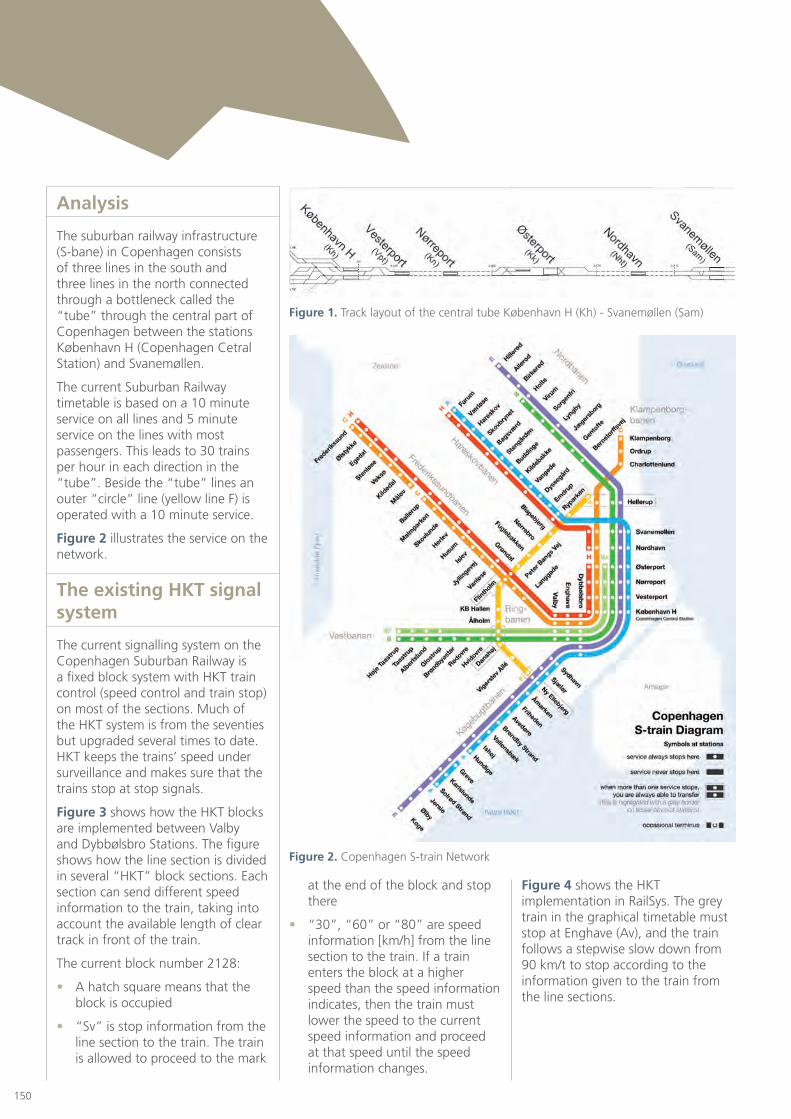
150
Analysis
The suburban railway infrastructure (S-bane) in Copenhagen consists of three lines in the south and three lines in the north connected through a bottleneck called the “tube” through the central part of Copenhagen between the stations København H (Copenhagen Cetral Station) and Svanemøllen.
The current Suburban Railway timetable is based on a 10 minute service on all lines and 5 minute service on the lines with most passengers. This leads to 30 trains per hour in each direction in the “tube”. Beside the “tube” lines an outer “circle” line (yellow line F) is operated with a 10 minute service.
Figure 2 illustrates the service on the network.
The existing HKT signal system
The current signalling system on the Copenhagen Suburban Railway is a fixed block system with HKT train control (speed control and train stop) on most of the sections. Much of the HKT system is from the seventies but upgraded several times to date. HKT keeps the trains’ speed under surveillance and makes sure that the trains stop at stop signals.
Figure 3 shows how the HKT blocks are implemented between Valby and Dybbølsbro Stations. The figure shows how the line section is divided in several “HKT” block sections. Each section can send different speed information to the train, taking into account the available length of clear track in front of the train.
The current block number 2128:
• A hatch square means that the block is occupied
• “Sv” is stop information from the line section to the train. The train is allowed to proceed to the mark
Figure 1. Track layout of the central tube København H (Kh) - Svanemøllen (Sam)
Figure 2. Copenhagen S-train Network
at the end of the block and stop there
• “30”, “60” or “80” are speed information [km/h] from the line section to the train. If a train enters the block at a higher speed than the speed information indicates, then the train must lower the speed to the current speed information and proceed at that speed until the speed information changes.
Figure 4 shows the HKT implementation in RailSys. The grey train in the graphical timetable must stop at Enghave (Av), and the train follows a stepwise slow down from 90 km/t to stop according to the information given to the train from the line sections.

149 How can CBTC improve the service on a saturated railway system?
151
Systems Engineering
Figure 3. HKT step diagram from Valby (Val) passing Enghave (Av) to Dybbølsbro (Dbt)
Figure 4. HKT implementation in RailSys (Upper graph: Speed profile – Lower graph: Graphic timetable)
The future CBTC system
The future signalling system is a train control system based on radio communication instead of fixed signals at the side of the tracks as for existing signals.
CBTC uses moving block instead of fixed block as the existing HKT. The size of the moving block separating two trains takes into account their relative location and individual performance. Therefore, headway is minimised as compared to fixed blocks. It leads to an optimal use of the infrastructure by shortening headways, which is suitable for an urban rail system with a high frequency. The integrated CBTC system knows the position of each train very accurately. It can control the behaviour of the train at all times and, in response to changing conditions, can modify behaviour to ensure the safety of the trains while offering maximum service with a minimum number of failures. It can adapt its algorithms to take advantage of individual train behaviour, and change parameters to ensure optimum use of resources, such as platform availability and traction power. (e.g. Thales3).
The CBTC system will have moving blocks at all sections except point areas. The safety parameters for the new CBTC signal system used in this analysis are as follows:
Safety distance: 50 metres
Block lengths: 100 metres
Point setting time: 7 sec
CBTC signalling systems have been installed at numerous urban railway transit systems around the world both in brand new systems and lines, and as an upgrade of existing lines with old signalling systems to a new CBTC signalling system. For example in New York City on the Carnesie Line in the subway network there has been an upgrade of an existing interlocking to CBTC. It has been in revenue service since
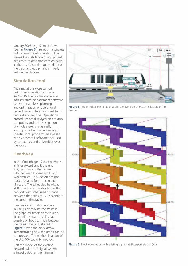
152
January 2006 (e.g. Siemens4). As seen in Figure 5 it relies on a wireless radio communication system. This makes the installation of equipment dedicated to data transmission easier as there is no continuous medium on the track and equipment is mostly installed in stations.
Simulation tool
The simulations were carried out in the simulation software RailSys. RailSys is a timetable and infrastructure management software system for analysis, planning and optimisation of operational procedures and facilities in rail traffic networks of any size. Operational procedures are displayed on desktop computers and the investigation of whole systems is as easily accomplished as the processing of specific, local problems. RailSys is a widely accepted software tool used by companies and universities over the world.
Headway
In the Copenhagen S-train network all lines except Line F, the ring line, run through the central tube between København H and Svanemøllen. This section has one track allocated for traffic in each direction. The scheduled headway at this section is the shortest in the network with scheduled distance between the trains at 120 seconds in the current timetable.
Headway examination is made in RailSys by moving the trains in the graphical timetable with block occupation shown, as close as possible without conflicts between the trains. This is illustrated in Figure 6 with the black arrow demonstrating how the graph can be compressed. The method is a part of the UIC 406 capacity method.
First the model of the existing network with HKT signal system is investigated by the minimum
Figure 5. The principal elements of a CBTC moving block system (Illustration from Siemens4)
Figure 6. Block occupation with existing signals at Østerport station (Kk)

149 How can CBTC improve the service on a saturated railway system?
153
Systems Engineering
Figure 7. Minimum headway with the existing signals and scheduled running time in central tube at the bottleneck Vesterport Station (Vpt)
technical headway in the central tube of 110 sec and a scheduled headway of 115 seconds.
By using the new CBTC system, the minimum technical headway at the central tube is reduced to 75 sec and a scheduled headway of 78 seconds. By comparing Figure 7 and Figure 8, it is clear that reductions in headway are mainly caused by a shorter length of clear track in front of the train, and this is most noticeable at stations.
Ninety seconds headway in the central tube
Based on previous headway analysis a timetable which has 90 seconds headway through the central tube has been evaluated.
Figure 9 shows a graphical timetable with 90 second headway, through the central tube on the infrastructure with the new CBTC signalling system (with block occupation around the trains). The station dwell times are the same as in the current timetable. The Figure shows there are no conflicts, with a buffer time between the trains.
The same timetable in the existing HKT signalling system in Figure 10 shows a timetable with many conflicts and no buffer time indicating 90 second headway in the current HKT system is not possible.
Only the headway in the central tube with the existing scheduled dwell times is analysed in this scenario. Where the trains are headed, where they will turn around and the trains’ stopping pattern outside the central tube are not analysed in this scenario.
The new CBTC signal system will make it possible to operate a timetable with 90 second headway in the central tube, though the punctuality of a timetable with this headway will be lower than a scenario with the current timetable implemented.
Figure 8. Minimum headway with CBTC signals and scheduled running time in the central tube at the bottleneck Østerport station (Kk)

154
Figure 9. Scenario with a 90 second headway timetable in the central tube with CBTC signals

149 How can CBTC improve the service on a saturated railway system?
155
Systems Engineering
to reach the same punctuality as the punctuality from the delay statistics.
The delay function in RailSys is implemented as an exponential distribution. The delay function uses at each station two parameters:
1. Percentages of delayed trains at the current stations with and without signal failures. The percentages of trains affected by an initial delay at all station are taken from the Banedanmark RDS data
2. Average delay was set to 1.2 minutes after calibration and maximum delay was set to 6.0 minutes after calibration, The average lateness and maximum lateness were calibrated to reach around the 96.7 % punctuality from 2008.
In the RailSys model punctuality for all stations on the Suburban Railway Network was 96.6%, which was close to the 96.7% real observed punctuality from the RDS data.
Multiple simulations
Both the current network and the network when a CBTC system is implemented have been simulated. The current train control system allows 100 seconds minimum
delays are due to the old signalling system.
The model for the delay data will be based on data from Rail Net Denmark. Delay data for 2008 were analysed and used in this model. These are divided into three different causes of the delayed train.
The new CBTC system will mainly remove the delays caused by signal failures. The delays are implemented in the RailSys model for the existing network and the model is calibrated
Delays
A train on the Copenhagen Suburban Railway is, according to the operator DSB and Rail Net Denmark, defined as delayed if the train is more than 2½ minute late. Therefore, this minimum delay is used in the punctuality analyses.
Today signalling failures are the cause of many train delays at most rail sections in Denmark. Many of those
Figure 10. Scenario with 90 second headway timetable in the central tube with existing signals
Figure 11. Amount of delays related to different groups
15+64+212008
Signals
Operator and external
Tracks

156
headway in the tube and planned 120 seconds headway. It is expected that the CBTC system will result in a 75 second minimum headway, but the results of the simulations show that the implementation of CBTC will result in much higher punctuality. The lower number of failures in the signalling system and the improved headway will together result in a much better performance.
The better performance of a CBTC system can be exploited to give a higher punctuality (B), a higher frequency (C) or both (D) as illustrated in Figure 12.
The question now is how close can we get to the capacity limit, when the current signalling system has changed to a modern CBTC system?
To show the impact of some different ways to increase the traffic in the network some different scenarios have been simulated and compared, where:
• As a reference the current suburban railway network with the current traffic was simulated
• The current situation plus a new line running through the tube and continues on a new single track line to the end station
• The current situation plus a new line running through the tube and continues on a new double track line to the end station.
All these cases result in a much lower punctuality compared with the current situation independent of the number of new tracks. Therefore, the traffic in the tube was isolated in the next phases of the simulations.
For this phase the scenario was based on the current traffic and then added a line, 3 extra trains per hour in each direction, which were only running in the tube and cut off at the end of the tube. The impact of the added line to the punctuality was nearly as big as the impact of the complete line as simulated before.
Figure 12. Illustration of capacity and punctuality
Figure 13. Simulation overview
Delay Data from statistics
CBTC system without signal failures
CBTC system without signal failures
Existing infrastructure with HKT signals
Existing HKT signals without signal failures
Calibration of model to reach real punctuality
Removing signal failures from input delay data
Removing signal failures from input delay data
New CBTC signal system

149 How can CBTC improve the service on a saturated railway system?
157
Systems Engineering
Roll out plan for the implementation of the CBTC signal system
According to Rail Network Denmark the implementation of the new CBTC signal system should be fully implemented in 2020 (e.g. Banedanmark5).
The signal programme will initially be provided by one supplier. The same supplier should thus provide and install the new signal system on the S-Bane - including the signal equipment to be installed inside the rolling stock.
The Remote System must be clear, so it can control train traffic when the new signal system is used on the first line. It kept open the tender for the supplier, whether to establish a new remote control system in a newly built centre, or whether the existing remote control system can be reused.
Figure 14. Results of the simulation
Figure 15. Roll out plan for the Signal Programme on the Copenhagen S-Bane network
All Failures
Perc
ent
of t
rain
s at
tim
e
RDS Data
Existing system model
Future CBTC model
Without signal failures
With all failures Without signal failures
Delay statistics 96.7 %
Model of existing network 96.5 % 97.7%
Model of future network with CBTC 99.0 % 99.2%

158
References
1. Kaas, A.H.; Landex, A.; Schittenhelm, B.; Schneider-Tilli, J. Practical use of the UIC 406 capacity leaflet by including timetable tools in the investigations Proc. Of the 2nd International Seminar on Railway Operations Modelling and Analysis, eds. I.A. Hansen, F.M.Dekking, R.M.P. Goverde, B. Hindergott, L.E. Meester, Hannover, 2007.
2. Kaas, A.H. & Landex, A., the most suitable travel speed for high frequency railway lines. Proc. Of the 1st International Seminar on Railway Opera¬tions Modelling and Analysis, eds. I.A. Hansen, F.M.Dekking, R.M.P. Goverde, B. Hindergott, L.E. Meester, The Netherlands, 2005.
3. Thales, Selftrac CBTC, Communications-Based Train Control For Urban Rail.
4. Siemens, Trainguard MT CBTC – The Moving Block Communications-Based Train Control Solution.
5. Banedanmark, Nye Signaler på Banen www.bane.dk.
The rollout of the new signalling takes place in four phases from the time the policy decision is taken:
• Tender
• Design of the new signaling
• Deploying and testing on the first section (Early Deployment)
• Rollout of the other lines.
The roll out on the S-Bane, will be in sections. First roll out (Early Deployment Project) will take place at the section between Hillerød and Jægersborg in 2014, where the new CBTC will be rigorously tested before being rolled out on other sections.
Conclusions
The conclusion of this simulation was that no extension of traffic through the tube is possible before the signalling system is changed to a high performance CBTC system, but some extensions are possible outside the tube.
Another finding from the investigations was a comparison between the effects of the new system running without failures against the effects of a new system with higher capacity. Here the conclusion was very clear – extra capacity within the CBTC system improves punctuality on the saturated system much more than having a future signalling system with no failures.

159

Technical Journal
09
www.atkinsglobal.com
© Atkins Ltd except where stated otherwise. The Atkins logo, ‘Carbon Critical Design’ and the strapline ‘Plan Design Enable’ are trademarks of Atkins Ltd.
PAPERS 135 - 149
Technical Journal
Papers 135 - 149
09