The All-pay Auction with Non-monotonic Payoff

Subhasish M. Chowdhury*

School of Economics, Centre for Behavioural and Experimental Social Science, and Centre for

Competition Policy, University of East Anglia, Norwich NR4 7TJ, UK.

Email: s.modak-chowdhury@uea.ac.uk

Abstract

We model innovation contests as an all-pay auction in which it is possible not to achieve

successful innovation despite costly R&D investments, and as a result, there is no winner. In such

a case the winning payoff turns out to be non-monotonic in own bid. We derive the sufficient

conditions for the existence of pure strategy equilibria, and fully characterize the non-degenerate

mixed strategy equilibrium. In the mixed strategy equilibrium, the support of the low-value bidder

is not continuous, and both the high-value and the low-value bidders place an atom in the (distinct)

lower bound of their respective support. Under symmetric valuation, both bidders place an atom

at zero. These results can explain why we do not observe very low quality innovation in real life,

or why even symmetric firms may stay out of an innovation contest.

JEL Classifications: C72, 74, D44, O30

Keywords: Innovation, All-pay auction, No-win, Non-monotonicity

* An earlier version of this study was circulated in 2009. I appreciate the useful comments of two anonymous referees,

Yeon-Koo Che, Dan Kovenock, Stephen Martin, Bill Novshek, Roman Sheremeta, Iryna Topolyan, the participants

at the ‘Contests and Innovation’ workshop in Anchorage, 20th Game Theory Festival at SUNYSB, Midwest Economic

Theory meetings at Iowa, 10th SAET Conference in Singapore, and the seminar participants at the Universities of

Cincinnati, East Anglia, Monash, Purdue, and Yonsei. Any remaining errors are mine alone.

2

1. Introduction

In an innovation contest, firms make costly R&D investments to innovate a new product or

process, and usually the highest quality innovation wins a patent or helps the owner firm to gain a

high market share. This procedure matches closely with a contest in which players have the

opportunity to make sunk investment of scarce resources in order to win prize(s). In specific, due

to its cutthroat nature, innovation tournaments and patent races can be modeled as an all-pay

auction – where bidders simultaneously bid for prize(s) and pay their bids irrespective of the

outcome. Because of its wide applications to electoral contests, rent-seeking activities, legal

disputes, in addition to patent races and innovation tournaments, the all-pay auction has been a

popular research tool. The equilibrium under complete information for the first-price all-pay

auction, in which a single prize is awarded with certainty to the highest bidder, is fully

characterized by Baye et al. (1996).1

Modeling an innovation contest as a standard all-pay auction, however, has its limitations

since it cannot explain certain phenomena in innovation. For example, non-participation of

symmetric players, or non-observability of very low quality innovation in a patent race cannot be

explained with a standard all-pay auction model. Furthermore, the intrinsic nature of an innovation

process incorporates two specific features that a standard all-pay auction fails to capture. First,

there are two types of uncertainties in an innovation process (Loury, 1979): (i) a competitor may

make a successful innovation before one does himself; and (ii) despite costly investments in R&D,

the innovation may fail to be successful. A standard all-pay auction cannot model the latter type

of risk. Second, the value of the prize in the innovation may depend on the level of investment.

One needs to apply an all-pay auction model with bid-dependent prize value in such situations.

In this study, we introduce an all-pay auction with complete information that incorporates

these features. This model introduces the possibility that even the highest bid, if it is below a certain

random threshold, may fail to win the prize and the prize value becomes concave in own bid. This,

in turn, results in a non-monotonic winning payoff in own bid. We characterize all Pure Strategy

Nash Equilibria (PSNE) and Mixed Strategy Nash Equilibrium (MSNE) under this structure. This

is one of the first attempts to characterize equilibria for all-pay auctions in which the payoff unction

1 Baye et al. (1996) show that if there are unique bidders with highest and second-highest value for the prize, then a

there exists no PSNE, but a symmetric MSNE exists. For more than two second-highest value bidders, a continuum

of asymmetric MSNE exists. See also Baye et al. (1993) and Hilman and Riley (1989).

3

is non-monotonic in own bid. The equilibrium results explain some of the phenomena in the

innovation process that a standard all-pay auction model with monotonic payoff cannot explain.

These two features (no-win, and bid dependent prize) discussed above are very common in

various situations including and beyond the innovation process. A prominent example of the no-

win case is a successful technological innovation that is not marketable. After making costly

investments, products such as jetpack and teleportation machine were invented in 1961 and in

1993. But due to non-marketability issues none of these returned any profit to the inventors

(Wilson, 2007). In another example, firms may expend costly resources to create a product

prototype and submit the same for a procurement auction (Che and Gale, 2003). However, the

demand-side may not like any of the prototypes and reject all. Furthermore, interest groups may

lobby a government to influence the details of regulations (Baye et al., 1993), yet the government

may issue regulations that do not favor any special interest group. Finally, several male may

compete to court a female. But, despite their effort, she might decide to choose none.2

Similarly, there are numerous practical situations when the valuation of the prize in an all-pay

auction is affected by the bid. An example of this is the dependence of a patent’s value on the

corresponding R&D expenditures. A firm may earn a patent on a particular product if it can

innovate that product before its rivals do. But, at the same time, the firm’s expected payoffs from

the patent is greater if the product is of higher quality due to a higher volume of R&D expenditure.3

Another example is the relationship between the size of the gains by lobbyists and the

corresponding lobbying expenses in rent-seeking. A lobby group might succeed in influencing

government decision by making more lobbying expenditure than its rivals; and at the same time

the degree of influence might well be affected by the amount of lobbying expenditure. An example

of this type in rent seeking (Tullock, 1980) is given by Amegashie (1999). Other examples include

singing contests (e.g. American Idol) and business plan competitions. The best singer or business

proposal wins the contest and at the same time a better performance gives a higher valued contract

to the winner. For similar examples in sports and labor, see Bos and Ranger (2014).

2 See Sozou and Seymour (2005) for failure in courtship efforts (giving gifts). Even animals expend a variety of costly

irreversible effort in terms of courtship dance, songs, use of pheromone, and physical contest with other males etc.

with the intention of mating a particular female (Daly, 1978 and Bastock, 2007). However, in the post courtship period,

it is possible that none from a set of competing males is able to mate with the particular female they intend to. 3 For example Wakelin (2001) show a positive relationship between R&D investment and productivity in the UK

manufacturing industry. Arora et al. (2008) find similar relationship between patent value and R&D investment in the

US manufacturing industry.

4

To our knowledge, Amegashie (2001) is the first to introduce an all-pay auction in which

the reward is a function of the bid and the payoff becomes non-monotonic in own bid. As a result,

there exists a PSNE where one bidder places a high bid and the other bidder abstains from bidding.

However, the parametric form of the payoff structure is very restrictive and the equilibria in mixed

strategies are not analyzed.4 The studies by Bos and Ranger (2014), and Sacco and Schmutzler

(2008) consider bid dependent prize value and are closely related to the current study. Bos and

Ranger (2014) construct a two-bidder all-pay auction where the prize value is increasing in own

bid in a non-decreasing returns-to-scale fashion. The authors, however, make a strong assumption

that makes the winning payoff monotonically decreasing in own bid. They characterize the unique

MSNE. Sacco and Schmutzler (2008) construct an 𝑛 −bidder model. They assume that the

winning prize value is an increasing concave function of own bid minus the second highest bid,

and that the cost is convex. They find conditions under which a PSNE exists. To solve the

equilibria in mixed strategies, they make a strong assumption of monotonically decreasing payoff

in bids. Both the studies find equilibrium mixed strategies similar to that of Baye et al. (1996).

Siegel (2009) constructs a general family of games called the ‘all-pay contests’. Specifically,

it is an 𝑛-bidder model in which the bidders are asymmetric in terms of their prize valuations and

cost functions. Nevertheless, even in this generic structure, the highest bidder wins a prize with

certainty and the winning payoff is assumed to be monotonically decreasing in own bid. Siegel

(2009) provides with a generic formula for the equilibrium payoffs and Siegel (2010) characterizes

the equilibrium strategies and participation rules for this game. Siegel (2014) considers the case of

our interest, with non-monotonic payoff, and characterizes the equilibrium payoffs. Nevertheless,

the characterization of equilibrium is not done. Finally, the current study is similar to the study by

Bertoletti (2016) who consider a known minimum bid in an all-pay auction whereas we consider

a stochastic minimum bid level. Later we compare and contrast the two studies side by side.

In this study we focus on the innovation contests as all-pay auction in which there is a

possibility that no bidder wins a prize with certainty; and the winning payoff is non-monotonic in

4 There are further examples of all-pay auction models in which the reward depends on the bid level. Kaplan et al.

(2003) construct a model where a higher reward as well as a higher cost is incurred with a choice of lower time. They

characterize equilibria under both symmetric and asymmetric valuations. Che and Gale (2006) model lobbying as an

all-pay auction and take into account a cap on bidding. This structure can also be employed for bid-dependent valuation

where the choice variable positively influences the cost as well as the prize value. Kaplan et al. (2002) construct an

incomplete information model where the prize is separable in bidder type. Araujo et al. (2008) also use an incomplete

information structure with a non-monotonic payoff and show the existence of a pure strategy Nash equilibrium.

5

own bid. The literature shows the existence of PSNE and characterizes the equilibrium payoff, but

does not characterize all the equilibria for this game. We fully characterize the PSNE and the non-

degenerate MSNE. In the MSNE the support of the low-value bidder is not continuous, and both

the high-value and the low-value bidders place an atom in the lower bound of their respective (and

different) support. Under symmetric valuation, both bidders place an atom at zero. These results

can explain the observed phenomena in innovation contests that the existing studies cannot.

2. The Model

2.1 Construction of the All-pay Auction with Non-monotonic Payoff

There are two bidders, 1 and 2, with value for a prize V1 and V2. Without loss of generality assume

V1≥ V2 > 0. The bidders make costly bids, x1and x2, and the lowest bidder never wins the prize.

It is also possible that none of them wins the prize reflecting the situation of the ‘no success’ case

of innovation driven by nature, or the quality standard of the buying party in a procurement auction

etc. We incorporate this by introducing a random bid threshold R̃ (Araujo et al., 2008; Bertoletti,

2016) with known, continuous and twice differentiable cumulative distribution function G(. ),

where G(0) = 0, G′(.) = g(.) > 0, and G′′(.) = g′(.) < 0. The winner is determined by the highest bid

that is higher than the random threshold R̃. We assume complete information.

Irrespective of the outcome, bidders bear cost according to a known, continuous and twice

differentiable cost function C(. ) that is increasing and weakly convex in own bid i.e., C(0) =

0, C′(.) = c(.) > 0, and C′′(.) = c′(.) ≥ 0. Hence, the payoff function of bidder 𝑡 (neglecting a tie) is:

πt(xt, x−t; R̃) = {Vt-C(xt) if xt > Max(x−t, R̃ )

-C(xt) otherwise (2.1)

The probability that bidder 𝑡 bids more than the random threshold R̃ is G(xt). Hence, the

expected payoff for bidder 𝑡, when he is the winner, is G(xt)Vt − C(xt), if xt > x−t, where – 𝑡 is

denoted as the bidder ‘not 𝑡’. G(. ) here captures the diminishing returns nature of the payoff

function. In case of a tie under asymmetric values (V1 > V2), if both bidders bid more than the

random threshold (R̃), then the highest value bidder, i.e., bidder 1 wins the prize. In the case of

common value (V1= V2), such a tie is resolved by a coin toss. Given these specifications, we can

rewrite the payoff function as:

6

πt(xt, x−t) = {

G(xt)Vt –C(xt) if (xt > x−t) or (xt = x−t) and (Vt > V−t)

G(xt) Vt

2–C(xt) if (xt = x−t) and (Vt = V−t)

–C(xt) Otherwise

(2.2)

Let us call the payoff at the winning state the ‘winning payoff’ and denote the same for bidder

𝑡 as Wt(xt). The losing payoff is Lt(xt). Hence Wt(xt) = G(xt)Vt − C(xt) and Lt(xt) = − C(xt).

Denote the game as Г(1,2; R̃). Also, call the graph of the winning (losing) payoff in the bid-payoff

space the winning (losing) curve.

2.2 Shape of the Winning Curves

It is relatively easy to establish the shape of the losing curve. The winning curves for both bidders

start from the origin and are strictly concave. If C′(0)/G′(0) > Vt (𝑡 = 1, 2) then the winning

payoff is negative; otherwise it is inverted U-shaped with a unique maximum: showing the non-

monotonicity. In the case of asymmetric valuation (V1> V2), the maximum winning payoff of

bidder 1 is strictly higher than that of bidder 2. If we denote the bid that maximizes the winning

payoff of bidder 𝑡 by xtWmax, then x1

Wmax > x2Wmax. As bid increases, eventually the winning

payoff becomes negative. If the maximum bid that can earn bidder 𝑡 a non-negative winning

payoff (‘reach’ in Siegel, 2009) is denoted by x̅t , then x̅1 > x̅2 . The proofs of these

characterizations are included in the Appendix (Claims 1 – 7). The diagrammatic representations

of the curves under the different cases are shown in Figures 1.1 to 1.3, and in Figure 2.

Given this, we characterize the equilibria of the game. Sections 2.3 and 2.4 deal with the

asymmetric value case (V1> V2) whereas Section 2.5 deals with the common value case (V1= V2).

2.3 Pure Strategy Equilibria under Asymmetric Values (𝐕𝟏> 𝐕𝟐)

Lemma 1. If (i) {C′(0)

G′(0)≥ V1} , or (ii) {

C′(0)

G′(0)∈ [V2, V1)} , or (iii) {

C′(0)

G′(0)< V2 and (x1

Wmax ≥ x̅2)},

then for the game Г(1,2; R̃) with (V1> V2) an equilibrium in pure strategies exists. Under condition

(i) the unique equilibrium strategies are (x1∗ , x2

∗) = (0,0), whereas under condition (ii) or (iii) the

unique equilibrium strategies are (x1∗ , x2

∗) = (x1Wmax, 0).

Proof: See the Appendix.

7

Figure 1.1 PSNE Case (i) Figure 1.2 PSNE Case (ii)

Figure 1.3 PSNE Case (iii)

Case (i) of Lemma 1 resembles the situation of a standard all-pay auction with a very high

reserve price. If the reserve price is higher than the highest valuation then the bidders bid zero.

Cases (ii) and (iii) combined together correspond to the result in which one firm stays out of the

innovation contest whereas the other firm spends a fixed amount. This idea is discussed in the

existing literature specifically for Case (ii) (Amegashie, 2001; Bertoletti, 2016). Nonetheless, there

are distinctions between the two cases that the earlier studies do not specify. First, in Case (ii) the

random threshold is so high that it is always unprofitable for the weaker firm to enter the market.

However, in Case (iii) it could have otherwise been profitable for the weaker firm to enter the

market, but since the stronger firm makes a large enough bid, the weaker one stays out. The policy

implications are also different for the two cases. In particular, a cap (< x̅2) on bidding can improve

participation and competition for case (iii), but not for case (ii). These two cases, unlike the

standard all-pay auction results, explain why in some situations only a single big company invests

on some particular type of R&D project and smaller companies do not.

Lt, Wt

xt

W2 W1 L1 = L2

𝑥1𝑊𝑚𝑎𝑥

Lt, Wt

xt

W2

W1

L1 = L2

x̅2 x1Wmax

L1 = L2

W2

W1

Wt, Lt

xt

8

Lemma 2. If C′(0)

G′(0)< V2 and (x1

Wmax < x̅2) then there exists no pure strategy Nash equilibrium

for the game Г(1,2; R̃) with (V1> V2).

Proof: See the Appendix.

Proposition 1. An equilibrium in pure strategies for the game Г(1,2; R̃) with V1 > V2 exists if and

only if any of the conditions (i) {C′(0)

G′(0)≥ V1} , or (ii) {

C′(0)

G′(0)∈ [V2, V1)} , or (iii) {

C′(0)

G′(0)<

V2 and (x1Wmax ≥ x̅2)} holds. Under condition (i) there exist unique equilibrium bids (x1

∗ , x2∗) =

(0,0) whereas under condition (ii) or (iii) the unique equilibrium bids are (x1∗ , x2

∗) = (x1Wmax, 0).

Proof: Lemmas 1 and 2 imply Proposition 1. ∎

Proposition 1 reconfirms that under non-monotonic payoff pure strategy Nash equilibria exist

(Amegashie, 2001; Sacco and Schmutzler, 2008; Araujo et al., 2008). Adding to these studies, we

show that there are two PSNE for which the high value bidder places a positive bid and the low

value bidder bids zero (cases (ii) and (iii)). Moreover, there is another PSNE, where both bidders

bid zero (case (i)). For all these PSNE, the payoff characterization results of Siegel (2014) hold.

2.4 Mixed Strategy Equilibria under Asymmetric Values (𝐕𝟏 > 𝐕𝟐)

Figure 2. No Pure Strategy Equilibrium

x̅1 x̅2 xt

W1 W2

L1 = L2

Wt, Lt

x1′ x2

Wmax x1Wmax

𝑜

9

Now we consider only the case of {C′(0)

G′(0)< V2 < V1and (x1

Wmax < x̅2)}, i.e., the case with no

PSNE (Figure 2) and fully characterize the MSNE. This proves the existence of equilibrium in

mixed strategies that follows also directly from Theorem 5 of Dasgupta and Maskin (1986). Note

also that the payoff characterization results of Siegel (2014) still hold. Hence, the equilibrium

payoff of bidder 1, π1∗ = W1(x̅2) > 0 and the equilibrium payoff of bidder 2, π2

∗ = 0.5

Let us define the No-arbitrage Bid Function (NBF) of bidder 𝑡 to keep the other bidder

indifferent as Ft(x). In Lemmas 3 to 19 we derive the NBFs as: F1(s) =C(s)

V2G(s) , and F2(s) =

C(s)+W1(x̅2)

V1G(s) and construct the shapes of the NBFs. The NBFs are drawn in Figure 3. The Lemmas

(3 to 19) and the corresponding proofs are in the Appendix.

Figure 3. No-arbitrage Bid Functions

It is apparent that the NBFs are not CDFs. In particular, F2(s) is not non-decreasing.

However, the capacity constrained pricing games (Osborne and Pitchick, 1986; Deneckere and

Kovenock, 1996) face similar obstacles, and following the techniques employed in such games the

NBFs remain the basis for the construction of equilibrium strategies. Let IF2(s) = Infx≥s(F2(x)) be

the non-decreasing floor of F2(s). Hence, IF2(s) equals F2(s) except for the interval [0, x2min).

5 This is because the sure payoff of bidder 1 is W1(x̅2). Therefore, if the expected payoff of bidder 1 is not at least as

high as W1(x̅2), then it is not an equilibrium. And it is not possible to win with certainty when bid is less than x̅2. So,

π1∗ = W1(x̅2) > 0. Similarly, bidder 2 can always earn a zero payoff by not submitting any bid, hence π2

∗ = 0.

xt

F1 Ft

1

O x1′ x2

min x̅2

F2

10

Note that this suggests a mass point at zero and a gap in the support between 0 and x2min for bidder

2. However, by assumption bidder 1 wins the prize in case of a tie. Hence, bidder 2 would lose

with certainty at s1 = x2min and his expected payoff at 𝑠1 = 𝑥2

min will become −C(x2min) < 0.

Thus, s1 = x2min cannot be in bidder 2's support. Hence the support for bidder 2 is (x2

min, x̅2)⋃{0},

and the support for bidder 1 is [x2min, x̅2].

Then Q2(s) = {IF2(s) for s ∈ (x2

min, x̅2]

1 for (s ≥ x̅2) along with the mass point at zero can be a best

response function for bidder 2 – if it is a CDF. Note that Q2(s) is non-decreasing, non-negative,

right continuous and is less than or equal to 1 for all 𝑠; hence, Q2(s) is a CDF and is also a strategy.

Given Q2, if bidder 1 is indifferent between all bids in the interval (0, x̅2], then 𝐹1would be an

equilibrium strategy, since it already makes bidder 2 indifferent between all bids in the interval,

and he earns a strictly lower payoff by deviating from Q2. However, since Q2 is strictly less than

𝐹2 over the interval [0, x2min), bidder 1 will attach zero probability to that interval. Since bidder 1

must set the strategy that keeps bidder 2 indifferent in the points of support, it will place a mass

point at x2min, the size of which equals F2(x2

min). Finally, bidder 1 will place zero probability to

bid more than x̅2.

Hence the best response of bidder 1 is: Q1(s) = {

0 for s < x2Min

F1(s) for x2Min < s < x̅2

1 for s ≥ x̅2

.

It is also easy to check that Q1(s) is non-decreasing, non-negative, right continuous, less

than or equal to 1 for all s; and hence, is a strategy. In the following proposition we show that

Q1(x) and Q2(x) constitute the unique mixed strategy Nash equilibrium of this game.

Proposition 2. The unique mixed strategy Nash equilibrium of the game Г(1,2; R̃) with

restrictions {C′(0)

G′(0)< V2 < V1 and (x1

Wmax < x̅2)} is characterized by the CDF pair Q1∗(s) and

Q2∗ (s). Where, the equilibrium CDF for bidder 1 is

Q1∗(s) = {

0 for s < x2min

C(s)

V2G(s) for s ∈ [x2

min, x̅2]

1 for s ≥ x̅2

i.e., there is an atom at x2min with size α1(x2

min) =C(x2

min)

V2G(x2min)

. The equilibrium CDF for bidder 2 is

11

Q2∗ (s) =

{

C(x2min) +W1(x̅2)

V1G(x2min)

for s ≤ x2min

C(s) +W1(x̅2)

V1G(s) for s ∈ (x2

min, x̅2]

1 for s ≥ x̅2

i.e., there is an atom at 0 with size α2(0) =C(x2

min)+W1(x̅2)

V1G(x2min)

.

Proof: We prove this proposition in two parts. First, we conclude that the pair {Q1(s), Q2(s)}

indeed characterizes an equilibrium. Then we show that the equilibrium is unique.

Note that Q1∗(s) = Q1(s) and Q2

∗ (s) = Q2(s). Therefore, from the previous discussion, Q1∗(s)

and Q2∗ (s) are strategies and are also best response to each other. Hence, the strategy pair

{Q1∗(s), Q2

∗ (s)} characterizes a mixed strategy Nash equilibrium for the game Г(1,2; R̃) . The

diagrammatic representation of the equilibrium is in Figure 4.

Figure 4. Equilibrium Distribution Functions

Now, if we show that the equilibrium support is unique, then the uniqueness of the equilibrium

will also be proved. It is clear that the supports of equilibrium distribution coincide and are equal

to the interval (x2min, x̅2]. In addition, bidder 2 has a mass point at 0. If s ∈ Support(Qt

∗) then for

any Ft ≠ Qt∗, the payoff of bidder 𝑡 when the other bidder plays equilibrium strategy,

πt(Ft(𝑠), Q−t∗ (s)) < πt

∗ . Also, if πt(Ft(𝑠), Q−t∗ (s)) > πt

∗ , then s ∉ Support(Qt∗) . Hence the

supports of the bidders’ mixed strategies are unique and so are the equilibrium mixed strategies.∎

Qt∗

Q1∗

1

xt O x̅2 x2min

Q2∗

12

Note three important features of this equilibrium, the first two of which are distinct from the

standard all-pay auction equilibrium. The high-value bidder places an atom at the lower bound of

his support, the low value bidder’s support is discontinuous, and although the equilibrium

distributions are different from the standard all-pay auction, the equilibrium payoffs of the bidders

are similar to the standard case and follow the payoff characterization results of Siegel (2014).

2.5. Characterization of Equilibria under Symmetric Value (𝐕𝟏 = 𝐕𝟐)

For the case of symmetric value (V1 = V1 = V) all-pay auction with non-monotonic payoff,

define x̅ = {x ≠ 0: C′(0)

G′(0)< 𝑉 & 𝑊(x) = 0}. It can easily be shown that for

C′(0)

G′(0)≥ V, the common

winning curve will start from zero and is always negative. Adhering to the similar analysis as in

the previous section, we derive the following proposition.

Proposition 3. A pure strategy equilibrium with unique equilibrium strategies (x1∗ , x2

∗) = (0,0)

exists for the game Г(1,2; R̃) with V1 = V2 = V if and only if C′(0)

G′(0)≥ V.

Figure 5.1 Symmetric Value Payoff Functions Figure 5.2 Symmetric Value Equilibrium CDFs

It can also be shown that for C′(0)

G′(0)< 𝑉 the common winning curve starts from zero and is

inverted U-shaped. Adhering to the similar analysis as in section 2.4, we derive the following

proposition. The proofs of Propositions 3 and 4 are obvious and are omitted.

Proposition 4. The unique mixed strategy Nash equilibrium of the game Г(1,2; R̃) with restriction

C′(0)

G′(0)< V1 = V1 = V is characterized by the common CDF Q∗(s), where

Q∗(x)

x x̅

1

0

Q(x)

0

Lt,Wt

x

L1 = L2

x̅ xWmax

𝑊1 = W2

13

Q∗(s) =

{

C′(0)/G′(0)

V for s = 0

C(s)

VG(s) for s ∈ (0, x̅]

1 for s ≥ x̅

.

i.e., the common support is [0, x̅] and in the equilibrium both the bidders place the same amount

of mass (C′(0)

VG′(0)) at 0. Both bidders earn zero payoff in the equilibrium.

In a standard 2-bidder all-pay auction the winning payoff is positive at zero-bid and is

monotonically decreasing. Hence, bidders do not place atoms at the same point in equilibrium. For

example, in Baye et al. (1996), if both bidders place atoms at zero, then shifting mass to a positive

bid is a profitable deviation for both the bidders. In contrast, under the current case the winning

curve starts from the origin and is continuous. Hence, if a bidder shifts a mass of ε > 0 above

zero, then its marginal payoff remains zero and as a result, the bidders do not have incentive to

shift mass from zero. This implies that in a contest between bidders with similar abilities

sometimes some bidders opt out of the contest. In the standard common value all-pay auction,

bidders do not place a mass point in equilibrium strategy, and as a result, it is not possible to

explain such observation with the standard all-pay auction results.

2.6. Overall Characterization of Equilibria

Theorem. Propositions 1 to 4 fully characterize the equilibria for the all-pay auction with non-

monotonic payoff described by the game Г(1,2; R̃).

Propositions 1 to 4 analyze mutually exclusive and exhaustive cases of the game Г(1,2; R̃).

The proof of the theorem is essentially the collection of the proofs of the four propositions.

3. Discussion

We model innovation contests as an all-pay auction in which the highest bid wins the contest only

when it is above a random threshold level. This structure captures both risk against rivals and risk

against nature in innovation contests. This model structure also allows us to investigate several

phenomena in innovation contest that could not be investigated with standard all-pay auction

model. The model structure makes the winning payoff non-monotonic in own bid, and, as a result,

this study is one of the first attempts to analyze the all-pay auction with non-monotonic payoff.

14

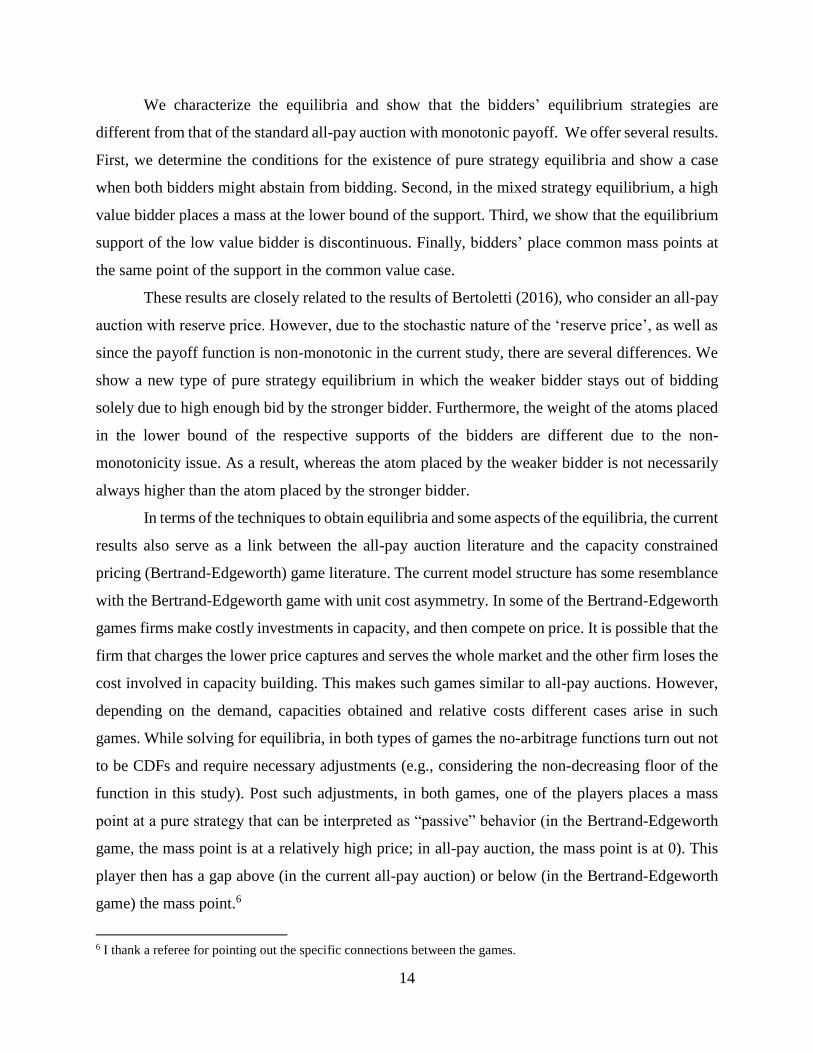
We characterize the equilibria and show that the bidders’ equilibrium strategies are

different from that of the standard all-pay auction with monotonic payoff. We offer several results.

First, we determine the conditions for the existence of pure strategy equilibria and show a case

when both bidders might abstain from bidding. Second, in the mixed strategy equilibrium, a high

value bidder places a mass at the lower bound of the support. Third, we show that the equilibrium

support of the low value bidder is discontinuous. Finally, bidders’ place common mass points at

the same point of the support in the common value case.

These results are closely related to the results of Bertoletti (2016), who consider an all-pay

auction with reserve price. However, due to the stochastic nature of the ‘reserve price’, as well as

since the payoff function is non-monotonic in the current study, there are several differences. We

show a new type of pure strategy equilibrium in which the weaker bidder stays out of bidding

solely due to high enough bid by the stronger bidder. Furthermore, the weight of the atoms placed

in the lower bound of the respective supports of the bidders are different due to the non-

monotonicity issue. As a result, whereas the atom placed by the weaker bidder is not necessarily

always higher than the atom placed by the stronger bidder.

In terms of the techniques to obtain equilibria and some aspects of the equilibria, the current

results also serve as a link between the all-pay auction literature and the capacity constrained

pricing (Bertrand-Edgeworth) game literature. The current model structure has some resemblance

with the Bertrand-Edgeworth game with unit cost asymmetry. In some of the Bertrand-Edgeworth

games firms make costly investments in capacity, and then compete on price. It is possible that the

firm that charges the lower price captures and serves the whole market and the other firm loses the

cost involved in capacity building. This makes such games similar to all-pay auctions. However,

depending on the demand, capacities obtained and relative costs different cases arise in such

games. While solving for equilibria, in both types of games the no-arbitrage functions turn out not

to be CDFs and require necessary adjustments (e.g., considering the non-decreasing floor of the

function in this study). Post such adjustments, in both games, one of the players places a mass

point at a pure strategy that can be interpreted as “passive” behavior (in the Bertrand-Edgeworth

game, the mass point is at a relatively high price; in all-pay auction, the mass point is at 0). This

player then has a gap above (in the current all-pay auction) or below (in the Bertrand-Edgeworth

game) the mass point.6

6 I thank a referee for pointing out the specific connections between the games.

15

Although we consider a two-player case, the analyses still provide with important and intuitive

results especially since it resembles several real life situations and can explain phenomena related

to the innovation process that the standard all-pay auction models cannot explain. For example,

the results from the pure strategy equilibria can explain why some firms might stay out of a

procurement bidding or a patent race even when there are only two competing firms. In specific,

case (ii) implies that a small company does not invest in R&D, even though it would find it

profitable if it was the only participant. The mixed strategy equilibrium with symmetry results

show that placing atoms at the same point may not be out of equilibrium behavior and explain the

inactivity of some of the firms in an innovation contest even when the bidders are of the same

efficiency. Moreover, in the mixed strategy equilibrium with asymmetry, the common support in

the mixed strategies that starts from a positive bid explains the reason why only sufficiently high

amounts of R&D investment are observed across different industries; or why only sufficiently high

quality of procurement samples in a procurement auction are submitted.

The current study is aimed at characterizing the equilibria of this model. One obvious idea for

further research would be to extend the model to 𝑛-bidders. Another policy related extension

would be to show the effects of caps on bidding. Finally, it will be intriguing to design non-

monotonic payoff all-pay auction experiments using the structure of this study.

References

Amegashie, J.A. (1999). The number of rent-seekers and aggregate rent-seeking expenditures: an

unpleasant result. Public Choice, 99, 57–62.

Amegashie, J.A. (2001). An all-pay auction with a pure-strategy equilibrium. Economics Letters.

70, 79-82.

Araujo, A., de Castro, L.I., & Moreira, H. (2008). Non-monotoniticies and the all-pay auction tie-

breaking rule, Economic Theory, 35(3), 407-440.

Arora, A., Ceccagnoli, M., & Cohen, W. M. (2008). R&D and the patent Premium. International

Journal of Industrial Organization, 26, 1153–1179.

Bastock, M. (2007). Courtship: an ethological study. Aldine Transaction, Chicago.

Baye, M. R., Kovenock, D., & de Vries, C. G. (1993). Rigging the Lobbying Process: An

Application of the All-Pay Auction. American Economic Review, 83, 289-294.

Baye M.R., Kovenock D., & de-Vries C.G. (1996). The all-pay auction with complete information.

Economic Theory, 8, 1-25

Bertoletti, P. (2016). Reserve prices in all-pay auctions with complete information. Research in

Economics, 70(3), 446-453.

16

Bos, O., & Ranger, M. (2014). All-Pay Auctions with Polynomial Rewards. Annals of Economics

and Statistics/Annales d'Économie et de Statistique, (115-116), 361-377.

Che, Y., & Gale, I. (2003). Optimal Design of Research Contests. American Economic Review,

93(3), 646—71.

Che, Y., & Gale, I. (2006). Caps on Political Lobbying: Reply. American Economic Review, 96(4),

1355-60.

Daly, M. (1978). The cost of mating. American Naturalist, 112, 771–774.

Dasgupta, P., & Maskin, E.S. (1986). The Existence of Equilibrium in Discontinuous Economic

Games, I: Theory. Review of Economic Studies, 83(1), 1-26.

Deneckere R.J., & Kovenock, D. (1996). Bertrand-Edgeworth duopoly with unit cost asymmetry.

Economic Theory, 8(1), 1-25.

Hillman, A., & Riley, J. (1989). Politically contestable rents and transfers. Economics and Policy,

1, 17–39.

Kaplan, T. R., Luski, I., Sela, A., & Wettstein, D. (2002). All-pay auctions with variable rewards.

Journal of Industrial Economics, 4, 417–430.

Kaplan, T.R., Luski I., & Wettstein D. (2003). Innovative activity and sunk cost. International

Journal of Industrial Organization, 21, 1111 - 1133

Loury, G. C. (1979). Market Structure and Innovation. The Quarterly Journal

of Economics, 93 (3), 395-410.

Osborne, M., & Pitchik, C. (1986). Price competition in a capacity-constrained duopoly. Journal

of Economic Theory, 38, 238-260

Sacco, D., & Schmutzler, A. (2008). All-Pay Auctions with Negative Prize Externalities: Theory

and Experimental Evidence. The Berkeley Electronic Press working paper

Siegel R. (2009). All-Pay Contests. Econometrica, 77(1), 71-92.

Siegel, R. (2010). Asymmetric contests with conditional investments. The American Economic

Review, 100(5), 2230-2260.

Siegel, R. (2014). Contests with productive effort. International Journal of Game Theory, 43(3),

515-523.

Sozou P.D., and Seymour R.M. (2005). Costly but worthless gifts facilitate courtship. Proceedings

of the Royal Society of London, Series B, 272, 1877–1884.

Tullock, G. (1980). Efficient Rent Seeking. In James M. Buchanan, Robert D. Tollison, Gordon

Tullock, (Eds.), Toward a theory of the rent-seeking society. College Station, TX: Texas A&M

University Press, 97-112.

Wakelin, K. (2001). Productivity growth and R&D expenditure in UK manufacturing firms.

Research Policy, 30, 1079-1090.

Wilson, D. H. (2007). Where's My Jetpack?: A Guide to the Amazing Science Fiction Future that

Never Arrived. Bloomsbury USA.

17

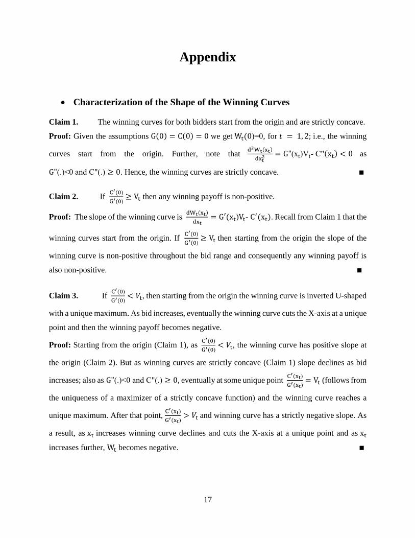
Appendix

Characterization of the Shape of the Winning Curves

Claim 1. The winning curves for both bidders start from the origin and are strictly concave.

Proof: Given the assumptions G(0) = C(0) = 0 we get Wt(0)=0, for 𝑡 = 1, 2; i.e., the winning

curves start from the origin. Further, note that d2Wt(xt)

dxt2 = G"(xt)Vt- C"(xt) < 0 as

G"(.)<0 and C"(.) ≥ 0. Hence, the winning curves are strictly concave. ∎

Claim 2. If C′(0)

G′(0)≥ Vt then any winning payoff is non-positive.

Proof: The slope of the winning curve is dWt(xt)

dxt= G′(xt)Vt- C

′(xt). Recall from Claim 1 that the

winning curves start from the origin. If C′(0)

G′(0)≥ Vt then starting from the origin the slope of the

winning curve is non-positive throughout the bid range and consequently any winning payoff is

also non-positive. ∎

Claim 3. If C′(0)

G′(0)< 𝑉t, then starting from the origin the winning curve is inverted U-shaped

with a unique maximum. As bid increases, eventually the winning curve cuts the X-axis at a unique

point and then the winning payoff becomes negative.

Proof: Starting from the origin (Claim 1), as C′(0)

G′(0)< 𝑉t, the winning curve has positive slope at

the origin (Claim 2). But as winning curves are strictly concave (Claim 1) slope declines as bid

increases; also as G"(.)<0 and C"(.) ≥ 0, eventually at some unique point C′(xt)

G′(xt)= Vt (follows from

the uniqueness of a maximizer of a strictly concave function) and the winning curve reaches a

unique maximum. After that point, C′(xt)

G′(xt)> 𝑉t and winning curve has a strictly negative slope. As

a result, as xt increases winning curve declines and cuts the X-axis at a unique point and as xt

increases further, Wt becomes negative. ∎

18

Claim 4. Starting with no-difference, W1 and W2 diverge away from each other and the

difference tends to the value difference (V1 − V2) as bid increases to infinity.

Proof: From the properties of G(x) , (W1 −W2)=G(x)(V1 − V2). Hence, (W1 -W2)|0 = (V1 −

V2)G(x)|0 = 0 . Also, d(W1−W2)

dxt= G′(xt)(V1 − V2)>0 and

d2(W1−W2)

dxt2 = G′′(xt)(V1 − V2)<0 .

Finally, limx→∞

(W1 −W2) = (V1 − V2) limG(x) =x→∞

(V1 − V2). ∎

Claim 5. If C′(0)

G′(0)< 𝑉2, define xt

Wmax = argmax(Wt(xt)); then x1Wmax ≥ x2

Wmax.

Proof: From Claim 3, argmax(Wt(xt)) is the solution to the first order condition dWt(xt)

dxt=

G′(xt)Vt-C′(xt) = 0 or C′(xt)

G′(xt)= Vt. Define K(xt)=

C′(xt)

G′(xt) . Note that

d(C′(xt)

G′(xt))

dxt> 0, hence the inverse

of K(xt) exists and is also a monotonically increasing function. Define K−1(.)=H(.) ; thus,

argmax(Wt(xt)) = H(Vt). By assumption V1≥ V2 and by construction H(.) is a monotonically

increasing function, hence x1Wmax ≥ x2

Wmax. ∎

Claim 6. maxW1 ≥ maxW2.

Proof: From Claim 5, maxWt = G(H(Vt))Vt − C(H(Vt)). Hence dmaxWt

dVt= G′(. )H′(. )Vt +

G(. ) − C′(. )H′(. ) = H′(. )[G′(. )Vt − C′(. )] + G(. ) = G(. ) > 0 as [G′(. )Vt − C

′(. )] = 0 for

maximization and Vt > 0 𝑓𝑜𝑟 𝑡 = 1, 2 . Given V1≥ V2, we confirm maxW1 ≥ maxW2. ∎

Claim 7. Define x̅t = {xt ≠ 0: C′(0)

G′(0)< Vt & Wt(xt) = 0} i.e., x̅t is the unique positive bid

by bidder t (Claim 3) for which his/her winning payoff is zero. 7 Then x̅1 > x̅2.

Proof: From Claim 4, (W1(x) −W2(x)) > 0 ∀ 𝑥 > 0 and by definition Wt(x̅t) = 0 .

Consequently, W1(x̅2) > W2(x̅2) = 0 = W1(x̅1). Hence, the inverted U-shape of winning curve

W1(. ) (Claim 3) confirms x̅1 > x̅2. ∎

These claims together constitutes the shape of the winning curves.

7 x̅t is defined as the ‘reach of bidder 𝑡’ in Siegel (2009 a, b)

19

Proofs of Lemmas 1 to 19.

Lemma 1. An equilibrium in pure strategies for the game Г(1,2; R̃) exists under condition (i)

{C′(0)

G′(0)≥ V1} or (ii) {

C′(0)

G′(0)∈ [V2, V1)} or (iii) {

C′(0)

G′(0)< V2 and (x1

Wmax ≥ x̅2)} . Moreover, under

condition (i) the unique equilibrium bids are (x1∗ , x2

∗) = (0,0), whereas under condition (ii) or (iii)

the unique equilibrium bids are (x1∗ , x2

∗) = (x1Wmax, 0).

Proof: (i) If C′(0)

G′(0)≥ V1 then by Claim 2 the winning payoffs are always non-positive and bidding

any positive amount with positive probability ensures loss. So, in equilibrium both the bidders bid

zero, i.e., x1∗ = x2

∗ = 0 . (ii) If C′(0)

G′(0)∈ [V2, V1) then bidder 2’s winning payoff is always non-

positive and following the same logic as in (i), x2∗ = 0. Bidder 1’s winning curve is inverted U-

shaped and given bidder 2 bids 0 with certainty, bidder 1 maximizes its payoff by always bidding

x1∗ = argmax(W1(x1)) = x1

Wmax > 0 . (iii) If C′(0)

G′(0)< V2 , then in some sufficiently small

neighborhood of zero bid, the winning payoff is positive for both bidders. When (x1Wmax ≥ x̅2)

then knowing bidder 2 never bids at or over x̅2 (as that will result in a negative payoff whereas a

zero-bid ensures a zero payoff), any bid between x̅2 and x̅1 gives a sure positive payoff to bidder

1. The sure payoff reflected by the winning curve is maximized at x1Wmax. Hence, bidder 1 bids at

x1∗ = x1

Wmax > x̅2 with certainty. Knowing this, bidder 2 bids x2∗ =0 with certainty. ∎

Lemma 2. If C′(0)

G′(0)< V2 and (x1

Wmax < x̅2) then there exists no pure strategy Nash equilibrium

for the game Г(1,2; R̃).

Proof: We prove the non-existence of PSNE by the way of contradiction. Suppose there exists a

PSNE {x̂1, x̂2}. Note first that x̂1 = x̂2 = 0 is not an equilibrium as any of the bidder 𝑡 can bid

xtWmax. Similarly, bidder 𝑡 bidding xt

Wmax and the other bidding 0 cannot be an equilibrium either,

as the other bidder can make a positive payoff by bidding 𝑥−𝑡 = xtWmax + 𝜀. It is not possible in

the equilibrium that x̂1 < x̂2, as x̅1 ≥ x̅2. It is also not possible x̂1, x̂2 > x̅2 as bidder 2 will never

bid more than x̅2, and knowing that bidder 1 will never bid more than x̅2 either. Hence, the possible

PSNE can be only in the range x̅2 ≥ x̂1 ≥ x̂2 > 0. Suppose, now that bidder 1 bids x̅2, then the

best response of bidder 2 is to bid 0. But if bidder 2 bids 0, then the best response of bidder 1 is to

bid x1Wmax. We know, however, that is not an equilibrium and bidder 2 will bid x1

Wmax + 𝜀. Bidder

20

1 in such a case will out bid bidder 2 and will keep on increasing the bid until x1 = x̅2. But then

the whole cycle starts again and no {x̂1, x̂2} can constitute a PSNE. ∎

In the following we first define and derive the no-arbitrage bid functions, and then derive the

equilibrium strategies from the no-arbitrage bid functions.

Lemma 3. Denote s̅t = inf{x: Ft(x) = 1} and st = sup{x: Ft(x) = 0}, then 0 ≤ st ≤ s̅t ≤ x̅t .

Proof: 0 ≤ st, as by assumption bids cannot be negative. st ≤ s̅t comes from the definitions of st

and s̅t and strict inequality holds if there is no pure strategy for any of the bidders. By definition

s̅t = inf{x: Ft(x) = 1}. If bidder 𝑡 places a mass on any bid more than x̅t then it will make a sure

negative payoff for that mass and as a result the expected payoff will fall. He can always increase

the expected payoff by placing that mass at 0. ∴ s̅t ≤ x̅t. ∎

Lemma 4. s̅t ≤ x̅2.

Proof: From Lemma 3, s̅2 ≤ x̅2. At x̅2 bidder 1 earns a sure payoff of W1(x̅2). 8 Therefore at x̅2,

The No-PSNE case implies x1Wmax < x̅2, hence W1(. ) is falling at x̅2 and placing any bid above

x̅2 with positive probability strictly reduces expected payoff for bidder 1. So, bidder 1 never places

a bid above x̅2, i. e. , s̅1 ≤ x̅2 as well. ∎

Lemma 5. Define x1′ = {x ≠ x̅2 ∶ W1(x) = W1(x̅2)}, then x1

′ < x1Wmax(< x̅2).

Proof: From Claim 3, W1(x) curve is inverted U shaped and from the definition of x1′ , W1(x1

′ ) =

W1(x̅2). Given the stated condition of no PSNE x1Wmax < x̅2 , we must have x1

′ < x1Wmax. Note

that the strict concavity property of G(. ) function ensures a unique x1′ . ∎

Lemma 6. s1 > x1′ .

Proof: Lemma 5 (x1′ < x1

Wmax) implies that at x1′ , W1(. ) is increasing. Hence, if bidder 1 bids

x1 ≤ x1′ with positive probability, then W1(x1) ≤ W1(x1

′ ) = W1(x̅2), and there is a chance that

bidder 1 will lose. But Bidder 1 can always bid x̅2 to earn a sure payoff of W1(x̅2). i.e., bidding

any amount ≤ x1′ provides less payoff to bidder 1 than the sure payoff. Thus, bidder 1 never places

a positive probability to bids up to x1′ , implying s1 > x1

′ . ∎

8 W1(x̅2) is the ‘power’ of bidder 1 as in Siegel (2009).

21

Lemma 7. In equilibrium, the support of bidder 2's distribution is contained in 0 and (x1′ , x̅2] .

Proof: From Lemma 6, s1 > x1′ . Knowing this, bidder 2 also never places a positive probability

in (0, x1′ ] as that ensures a negative payoff. So, bidder 2 places positive probability of bidding in

either 0 or between (x1′ , x̅2], i.e., bidder 2’s support is contained in 0 and(x1

′ , x̅2]. ∎

Lemma 8. s2=0.

Proof: From Siegel (2014), π1∗ > 0 and π2

∗=0. Combining with the fact that bidder 1 must win

with positive probability over the whole support to attain π1∗ > 0 we must have s2=0. ∎

Lemma 9. s̅1 = x̅2.

Proof: This comes directly from Siegel (2014). ∎

Lemma 10. s̅2 = x̅2.

Proof: From Lemma 4, s̅2 ≤ x̅2 and from Lemma 9, s̅1 = x̅2. Suppose s̅2 < x̅2 then because

W1(. ) is decreasing at x̅2 , placing any bid x1 ∈ [s̅2, x̅2) ensures bidder 1 a sure payoff of

W1(x1) > W1(x̅2): a contradiction with Siegel (2014). Hence s̅2 = x̅2. ∎

Lemma 11. F2(s1) = F2(0).

Proof: Suppose not. Then bidder 2 places a positive probability of bidding in the semi-open

interval (0, s1]. But that ensures a negative payoff which is contradictory to Siegel (2014). ∎

Lemma 12. Bidder 1’s support is connected on the interval (s1, x̅2).

Proof: Suppose not and there is a gap (𝑎, 𝑏) ⊆ (𝑠1, �̅�2), where 𝑏 > 𝑎; the gap can be a singleton. In

equilibrium bidder 1 earns the same expected payoff in every point of (s1, 𝑎) ∪ (𝑏, x̅2). But with

this gap bidder 1 can shift mass from Nε+(𝑏) to point 𝑎. In such a case his probability of winning

remains the same but cost goes down; and as a result payoff at Nε+(𝑏) goes up – which is a

contradiction. Hence, the support cannot have gap. ∎

Lemma 13. Support of F2 is contained in Support of F1 ∪ {0}.

Proof: Suppose not. Then the support of F2 includes at least parts of interval (x1′ , s1). However,

that is contradictory to Lemma 11. ∎

22

Lemma 14. If αt(s) is the amount of mass bidder 𝑡 places at point s, then α2(0) ∈ (0,1).

Proof: From Lemma 11, Prob(x2 < s1) = α2(0). ∴ π1(s1) = α2(0)G(s1)V1 − C(s1). Hence, if

α2(0) = 0 then π1(s1) = −C(s1) < W1(x̅2) and if α2(0) = 1 then bidding any x1 ∈ (x1′ , x̅2)

ensures bidder 1 a payoff W1(x1) > W1(x1′ ) = W1(x̅2) both of which are contradictory with

Lemma 8. ∴ α2(0) ∈ (0,1). ∎

Lemma 15. α1(s1) ∈ (0,1).

Proof: From Lemma 6, s1 > 0 and from Lemma 14, α2(0) > 0. If α1(s1) = 0, then given

Lemmas 12 and 13, at s1 bidder 2 loses with certainty and payoff of bidder 2 becomes – C(s1) <

0; and if α1(s1) = 1 then for any small ε > 0, bidding (s1 + ε) gives bidder 2 a sure payoff of

W2(s1 + ε) > 0: both of which are contradictory with Siegel (2014). ∴ α1(s1) ∈ (0,1). ∎

Lemma 16. A No-arbitrage Bid Function (NBF) of bidder 1 to keep bidder 2 indifferent is:

F1(s) =C(s)

V2G(s) , and an NBF of bidder 2 to keep bidder 1 indifferent is: F2(s) =

C(s)+W1(x̅2)

V1G(s) .

Proof: To keep bidder 1 indifferent, bidder 2 places the bid function F2(. ) in a way such that

F2(s)V1G(s) − C(s) = π1∗ = W1(x̅2). Solving for F2(. ) yields the NBF of bidder 2: F2(s) =

C(s)+W1(x̅2)

V1G(s). Similarly, bidder 1 places the bid function F1(. ) in a way such that F1(s)V2G(s) −

C(s) = π2∗ = 0. Solving for F1(. ) yields NBF of bidder 2: F1(s) =

C(s)

V2G(s). ∎

Lemma 17. lims→0

F1(s) < 1, F1(x1′ ) < 1, and F1(x̅2) = 1.

Proof: Using L’Hospital rule: lims→0

F1(s) =lims→0

dC(s)

ds

lims→0

d(V2G(s))

ds

=C′(0)

V2G′(0)< 1 as

C′(0)

G′(0)< V2.

Also, F1(x1′ ) =

C(x1′ )

V2G(x1′ )=

C(x1′ )

{V2G(x1′ )−C(x1

′ )}+C(x1′ )=

x1′

W1(x1′ )+C(x1

′ )< 1 as W1(x1

′ ) = W1(x̅2) > 0.

Recall also that x̅2 is the ‘reach’ of bidder 2. By the definition of bidder 2’s reach C(x̅2)

V2G(x̅2)= 1.

Hence, F1(x̅2) = 1. ∎

Lemma 18. F1(s) is monotonically increasing in the closed interval [x1′ , x̅2].

Proof: From Lemma 17, F1(x̅2) > F1(x1′ ). If there exists no extreme point of F1(. ) within the

open interval (x1′ , x̅2) then it means that F1(s) is monotonically increasing in (x1

′ , x̅2). In any

23

extreme point of F1(s), dF1(s)

ds=

V2G(s)C′(s)−C(s)V2G

′(s)

[V2G(s)]2= 0, i.e., [G(s)C′(s) − C(s)G′(s)] = 0. But,

[G(s)C′(s) − C(s)G′(s)] is a strictly upward rising curve from origin since [G(s)C′(s) −

C(s)G′(s)]|0 = 0 , and d[G(s)C′(s)−C(s)G′(s)]

ds= G(s)C"(s) − C(s)G"(s) > 0 ∀s > 0 . Hence, there is no

solution except origin for [G(s)C′(s) − C(s)G′(s)] = 0 , and there exists no extreme point for

F1(s) within the interval(x1′ , x̅2). Thus, F1(s) is monotonically increasing in [x1

′ , x̅2]. ∎

Lemma 19. F2(s) starts from infinity, monotonically decreases to 1 at s = x1′ , reaches unique

minimum within the open interval (x1′ , x̅2) and then monotonically increases to 1 at s = x̅2.

Proof: From Lemma 16, F2(s) =C(s)+W1(x̅2)

V1G(s). ∴ F2(0) = ∞ . And F2(x1

′ ) =C(x1

′ )+W1(x̅2)

V1G(x1′ )

=

C(x1′ )+W1(x1

′ )

V1G(x1′ )

=C(x1

′ )+{V1G(x1′ )−C(x1

′ )}

V1G(x1′ )

= 1. Also, F2(x̅2) =C(x̅2)+W1(x̅2)

V1G(x̅2)=

C(x̅2)+{V1G(x̅2)−C(x̅2)}

V1G(x̅2)= 1.

If we prove that F2(. ) is decreasing at x1′ then there will be at least one minimum point of F2(. ) in

the open interval (𝑥1′ , �̅�2). Note that

dF2(s)

ds=

V1G(s)C′(s)−{C(s)+W1(x̅2)}V1G

′(s)

[V1G(s)]2. Hence

𝑆𝑖𝑔𝑛 (dF2(s)

ds) = 𝑆𝑖𝑔𝑛(G(s)C′(s) − {C(s) +W1(x̅2)}G

′(s)) . At point x1′ , it can be shown that

Sign (dF2(s)

ds|x1′ ) = Sign(C′(x1

′ ) − V1G′(x1′ )) = Sign (−

dW1(s)

ds|x1′ ) < 0 as W1(. ) is upward

rising at point x1′ (Claim 3 and Lemma 5). Thus F2(. ) is decreasing at x1

′ and consequently, there

exists at least one minimum point of F2(. ) in the open interval (x1′ , x̅2).

Now, if we show that the minimum is unique then we will prove that (i) F2(. ) decreases from

infinity to 1 at x1′ and (ii) the minimum is in the interval (x1

′ , x̅2) . At a minimum, dF2(s)

ds= 0, which

implies (G(s)C′(s)−C(s)G′(s))

G′(s)= W1(x̅2). Here RHS is a positive constant whereas LHS is an upward

rising curve from origin.9 Thus there exists unique solution for (G(s)C′(s)−C(s)G′(s))

G′(s)= W1(x̅2), i.e.,

there exists unique minimum for F2(. ). Because F2(x1′ ) = F2(x̅2) = 1 and F2(s) is decreasing at

x1′ , ∴ argmin(F2(s)) = x2

min ∈ (x1′ , x̅2). ∎

These lemmas constitutes the shape of the NBFs that remain the basis of the equilibrium strategies.

9 Note that (G(s)C′(s)−C(s)G′(s))

G′(s)|0 = 0 and

d[(G(s)C′(s)−C(s)G′(s))/G′(s)]

ds=

G(s)[G′(s)C′′(s)−C′(s)G′′(s)]

[G′(s)]2> 0