towards regional projections of twenty-ﬁrst century sea ... · change based on ipcc sres...

Towards regional projections of twenty-first century sea-levelchange based on IPCC SRES scenarios

A. B. A. Slangen • C. A. Katsman • R. S. W. van de Wal •

L. L. A. Vermeersen • R. E. M. Riva

Received: 11 October 2010 / Accepted: 22 March 2011 / Published online: 5 April 2011

� The Author(s) 2011. This article is published with open access at Springerlink.com

Abstract Sea-level change is often considered to be

globally uniform in sea-level projections. However, local

relative sea-level (RSL) change can deviate substantially

from the global mean. Here, we present maps of twenty-first

century local RSL change estimates based on an ensemble of

coupled climate model simulations for three emission sce-

narios. In the Intergovernmental Panel on Climate Change

Fourth Assessment Report (IPCC AR4), the same model

simulations were used for their projections of global mean

sea-level rise. The contribution of the small glaciers and ice

caps to local RSL change is calculated with a glacier model,

based on a volume-area approach. The contributions of the

Greenland and Antarctic ice sheets are obtained from IPCC

AR4 estimates. The RSL distribution resulting from the land

ice mass changes is then calculated by solving the sea-level

equation for a rotating, elastic Earth model. Next, we add the

pattern of steric RSL changes obtained from the coupled

climate models and a model estimate for the effect of Glacial

Isostatic Adjustment. The resulting ensemble mean RSL

pattern reveals that many regions will experience RSL

changes that differ substantially from the global mean. For

the A1B ensemble, local RSL change values range from

-3.91 to 0.79 m, with a global mean of 0.47 m. Although the

RSL amplitude differs, the spatial patterns are similar for all

three emission scenarios. The spread in the projections is

dominated by the distribution of the steric contribution, at

least for the processes included in this study. Extreme ice loss

scenarios may alter this picture. For individual sites, we find

a standard deviation for the combined contributions of

approximately 10 cm, regardless of emission scenario.

Keywords Regional sea level � Sea-level projections �Climate change

1 Introduction

In a warming climate, the global mean sea level is expected

to rise, which will have serious implications for coastal

communities (Nicholls and Cazenave 2010). Therefore,

sea-level change is a central research topic in climate

change studies. The Intergovernmental Panel on Climate

Change (IPCC) Fourth Assessment Report (AR4) (Meehl

et al. 2007b) presents projections for global sea-level

change of 0.21–0.48 m under the Special Report on

Emission Scenarios (SRES) A1B scenario for the period

1980–1999 to 2090–2099, excluding carbon cycle feed-

backs and excluding the recently observed dynamical

changes in ice sheets. Adding their estimate for the

dynamical effect of ice sheet mass loss yields a global

estimate of 0.20–0.61 m (Meehl et al. 2007b, Table 10.7).

However, the IPCC projections are limited to a global

mean value and do not consider the large regional varia-

tions induced by several processes. Possible causes of

regional variations include the gravitational effects result-

ing from land ice mass changes (e.g., Woodward 1887;

A. B. A. Slangen (&) � R. S. W. van de Wal

Institute for Marine and Atmospheric research Utrecht, Utrecht

University, Princetonplein 5, 3584 CC Utrecht, The Netherlands

e-mail: [email protected]

C. A. Katsman

Royal Netherlands Meteorological Institute (KNMI),

P.O. Box 201, 3730 AE De Bilt, The Netherlands

L. L. A. Vermeersen

Faculty of Aerospace Engineering, TU Delft,

Kluyverweg 1, 2629 HS Delft, The Netherlands

R. E. M. Riva

TU Delft, Kluyverweg 1, 2629 HS Delft, The Netherlands

123

Clim Dyn (2012) 38:1191–1209

DOI 10.1007/s00382-011-1057-6

Mitrovica et al. 2001), thermal expansion (e.g., Landerer

et al. 2007; Wijffels et al. 2008), ocean dynamics (e.g.,

Landerer et al. 2007; Yin et al. 2010) and Glacial Isostatic

Adjustment (GIA) (e.g., Farrell and Clark 1976; Peltier

2004). In this study we incorporate all these effects in a

local scenario using the IPCC SRES scenarios A1B, A2

and B1, to illustrate the importance of regional sea-level

(RSL) variations in a warming climate. Some processes are

better understood and modelled in these simulations than

others. In particular the ice sheet contributions used in

IPCC AR4 were acknowledged to have limitations and

possibly underestimate their future contributions (e.g.

Rignot et al. 2008a, b, 2011; Velicogna 2009). However,

we do apply them here to allow for a comparison of the

regional patterns with the well-known global mean IPCC

AR4 estimates.

Throughout this paper, all sea-level changes discussed

are relative sea-level changes. These are the changes

relative to the Earth’s surface, as measured by devices

attached to the surface, for instance tide gauges. Relative

sea-level change is different from absolute sea-level

change, which is the change with respect to the center of

mass of the Earth, as measured by air-borne devices such as

satellite altimeters.

Land ice mass changes represent a large contribution to

RSL change. Melt water from land ice does not distribute

uniformly over the ocean, due to gravitational effects and

induced changes in the shape and rotation of the Earth

(e.g., Vermeersen and Sabadini 1999). The gravitational

effect is the direct manifestation of Newtons law (mass

attracts mass), which implies that land ice attracts ocean

water. When ice melts, the gravitational attraction of the

ice sheet weakens, so the RSL drops near the ice (up to a

radius of *2,200 km), rises less than the global mean from

*2,200 to *6,700 km, and rises more than the global

mean at a larger radial distance. In addition, changes in

surface load (in this case represented by land ice masses

and the global ocean) cause a deformation of the Earth’s

surface, which in turn affects the Earth’s gravity field and

causes an additional redistribution of ocean water. This

coupling between surface mass changes and solid Earth

deformation, also known as self-gravitation, was already

described by Woodward (1887), but only implemented in a

numerical model by Farrell and Clark (1976), who intro-

duced the ‘‘Sea-Level Equation’’. This equation computes

both the sea-level change and the solid-Earth deformation

due to ice mass variations. In addition, ice melt and solid-

Earth deformation cause a redistribution of mass that

affects the Earth’s rotation rate and the position of its

rotation axis (e.g., Vermeersen and Sabadini 1999) and

hence the RSL change pattern (Milne and Mitrovica 1998).

Another large contribution to RSL change arises from

local changes in temperature and salinity of the seawater;

the thermosteric and halosteric contributions. Warming of

the ocean in response to rising atmospheric temperatures

results in an increase of volume and hence sea-level rise. A

higher salinity has the opposite effect, as it increases the

density of the ocean water. Like the RSL change resulting

from land ice mass changes, steric RSL changes (variations

in ocean temperature and salinity) are far from spatially

uniform (Cazenave and Nerem 2004). Although in many

places local thermosteric changes are dominant [see for

example Bindoff et al. (2007, Figure 5.15b)], changes in

ocean salinity can also lead to substantial local sea-level

variations (Antonov et al. 2002). These local steric changes

are closely linked to ocean circulation changes, as the latter

are driven by local density gradients (Meehl et al. 2007b,

Section 10.6.2).

In order to obtain regional patterns of RSL change, the

processes mentioned above need to be modelled. The first

component considered is the land ice contribution to RSL

change. For this contribution, the changes in the ice mass of

mountain glaciers and ice caps have been modelled by a

volume-area model (Bahr et al. 1997; Van de Wal and Wild

2001), to obtain, in contrast to the IPCC AR4, a regional

pattern of the glacier mass loss. Additionally, the mass

changes of the Greenland and Antarctic ice sheets have been

computed with model-derived relations between tempera-

ture and ice sheet mass change as outlined in IPCC AR4

(Meehl et al. 2007b). The magnitude and location of all land

ice mass changes serve as input for a sea-level model, which

calculates a gravitationally consistent field of RSL change

while accounting for rotational processes. The second

component considered is the steric component (i.e. changes

in ocean density and circulation), for which we use the

results of Atmosphere-Ocean coupled General Circulation

Models (AOGCM’s) provided in the Coupled Model

Intercomparison Project phase 3 (CMIP3) database (Meehl

et al. 2007a). The AOGCM’s provide a global mean and

local sea-level change relative to the mean due to circulation

changes resulting from temperature and salinity variations.

The third component added is the sea-level change resulting

from GIA, which is the present-day viscoelastic response of

the Earth’s crust to changes in ice masses throughout the last

glacial cycle. To model the influence of GIA on regional

sea-level change the result of the ICE-5G(VM2) glaciation-

deglaciation model (Peltier 2004) is used.

To allow for a comparison of the IPCC AR4 global

mean estimates (Meehl et al. 2007b) to the regional pat-

terns, all results presented in this study are, on purpose,

based on the same data as used in IPCC AR4. The only

exception is the use of a new data set for the contribution of

mountain glaciers and ice caps. The reason for this is that

the present study requires a data set that provides locations

and initial volume of the individual glaciers to calculate

regional scenarios for this contribution, while the IPCC

1192 A. B. A. Slangen et al.: Towards regional projections of twenty-first century sea-level change

123

data only provide a global value for all mountain glaciers

and ice caps combined. The outcome of this study is to be

considered as a first step towards the development of

regional projections for sea-level change, complementary

to the global mean projections in IPCC AR4. Although in

IPCC AR4 the self-gravitation effect is recognized as a

cause of regional RSL variations (Bindoff et al. 2007,

Section 5.5.4.4), it is not considered for the projections of

future sea-level change (Meehl et al. 2007b). Here we will

quantify this effect in detail. The local variations in steric

sea-level change were discussed in Meehl et al. (2007b).

Additionally to the contributions presented in IPCC AR4,

the influence of GIA on sea-level change is considered,

which can have very large effects locally.

This study is the first attempt to combine the three most

important components affecting sea-level change on a

regional scale, which has not been done before to our

knowledge. Scientifically all ingredients are available for

these three components to make the step from global pro-

jections to local projections and to provide specialized

information regarding RSL change, for which there is an

increasing demand from governments and policy makers.

There are some potential contributions to local RSL

variations that are not included in this study because of a

lack of appropriate data or model results. Examples are

surface movements due to tectonic effects or subsidence,

changes in storm surge height (although climatic changes

of wind direction and wind speed are included in the steric

contribution), water impoundment behind dams, ground-

water storage change and the influence of freshening due to

land ice melt on the ocean circulation. Hence, the results of

this study should be considered as a first attempt to con-

struct a regional projection for RSL change with room for

improvement as science progresses.

The paper is structured as follows. Section 2 describes

all models and the data used to construct the spatially

varying fields of RSL change. In Sect. 3 the results are

shown, for the separate contributions and for the total

projected RSL change. A discussion of the results is pre-

sented in Sect. 4 and finally in Sect. 5 the conclusions are

described.

2 Data and methodology

In this section, all models and data used in this study are

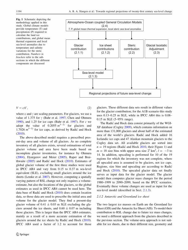
discussed. A schematic of the methodology applied to

construct the scenarios for local RSL change is presented

in Fig. 1. The land ice contribution is split up in two

components: the small mountain glaciers and ice caps

(Sect. 2.1.1), and the large ice sheets, Greenland and

Antarctica (Sect. 2.1.2). Both respond differently to cli-

matic changes and thus the ice mass changes need to be

modelled in a different way. Once the magnitude and

locations of all land ice mass changes are known, a sea-

level model is used to compute the local RSL pattern

resulting from the melting land ice. This is described in

Sect. 2.1.3. The spatial pattern of the steric contribution is

computed using global mean thermal expansion data and

local RSL anomalies due to temperature and salinity

variations (Sect. 2.2). To account for the present-day

response to ice mass changes after the Last Glacial

Maximum, a spatially varying field of GIA is taken from

the ICE-5G(VM2) model (Sect. 2.3), and added to the

other contributions. This results in spatial patterns of future

RSL change, which will be discussed in Sect. 3. This

section ends with a description of the coupled climate

models that provide most of the data used to calculate both

the land ice and the steric contributions (Sect. 2.4).

2.1 Land ice contribution

2.1.1 Mountain glaciers and ice caps

We use a glacier model to estimate the RSL change con-

tribution from mass changes of mountain glaciers and ice

caps (henceforth glaciers), which is defined as all land

ice apart from the Antarctic ice sheet and the Greenland ice

sheet. This model is based on volume-area scaling (e.g.,

Bahr et al. 1997; Van de Wal and Wild 2001; Radic et al.

2007, 2008). It computes the volume change of all glaciers,

sorted by region and surface area, while accounting for the

change of glacier area in time, temperature changes and

precipitation changes, by using the mass balance

sensitivity:

dV

dt¼Xn

j¼1

Xm

k¼1

Aðj; k; tÞ � DTsðj; tÞdBPðj;tÞ

dTs

�

þDTnsðj; tÞdBPðj;tÞ

dTnsþ DPðj; tÞ

� ð1Þ

In Eq. 1, glacier area A is summed over n regions and m

size bins (discussed below). The mass balance sensitivity

dBP(j,t) is a function of the local precipitation P using

values from Zuo and Oerlemans (1997), but also results

from changes in local summer temperature change (DTs)

(summer is JJA in northern hemisphere, DJF in southern

hemisphere) as well as non-summer temperature change

(DTns). T and P are taken from the AOGCM’s (Sect. 2.4)

using the nearest neighbour approach (Van de Wal and

Wild 2001). The imbalance of glaciers at present is

accounted for by starting the calculations in 1865, and

applying a temperature increase of 0:6�C=100 years over

the period 1865–1990.

The relation between volume V and area A for a glacier

is assumed to follow a power law (Bahr et al. 1997):

A. B. A. Slangen et al.: Towards regional projections of twenty-first century sea-level change 1193

123

V ¼ cAc; ð2Þ

where c and c are scaling parameters. For glaciers, we use a

value of 1.375 for c (Bahr et al. 1997; Chen and Ohmura

1990), and 1.25 for ice caps (Bahr et al. 1997). For c we

adopt the value of 0.2055 m3-2c for glaciers and

1.7026 m3-2c for ice caps, as derived by Radic and Hock

(2010).

The above-described model requires a prescribed pres-

ent-day area and volume of all glaciers. As no complete

inventory of all glaciers exists, several estimations of total

glacier volume and area have been made based on

incomplete glacier inventories, for instance by Ohmura

(2004), Dyurgerov and Meier (2005), Raper and Brai-

thwaite (2005) and Radic and Hock (2010). Estimates of

global glacier volume of the first three studies were used

in IPCC AR4 and vary from 0.15 to 0.37 m sea-level

equivalent (SLE), excluding small glaciers around the ice

sheets (Lemke et al. 2007). However, computing a spatially

varying pattern of RSL change not only requires a volume-

estimate, but also the locations of the glaciers, so the global

estimates as used in IPCC AR4 cannot be used here. The

data base of Radic and Hock (2010) does contain location

data, so those data are used to prescribe the initial area and

volume for the glacier model. They find a present-day

glacier volume of 0.41 ± 0.03 m SLE excluding the gla-

ciers around the ice sheets, and 0.60 ± 0.07 m including

those glaciers. This is larger than the IPCC AR4 estimates,

mainly as a result of a more accurate estimation of the

glaciers around the ice sheets by Radic and Hock (2010).

IPCC AR4 used a factor of 1.2 to account for those

glaciers. These different data sets result in different values

for the glacier contribution; for the A1B scenario this study

uses 0.13–0.25 m SLE, while in IPCC AR4 this is 0.08–

0.15 m SLE (5–95% range).

The Radic and Hock data consist primarily of the WGI-

XF database (Cogley 2009), which contains information on

more than 131,000 glaciers and about half of the estimated

area of the world’s glaciers. Radic and Hock added 16

Icelandic ice caps and 47 Alaskan mountain glaciers to the

Cogley data set. All available glaciers are sorted into

n = 19 regions (Radic and Hock 2010, their Figure 1) and

m = 18 size bins with upper area size 2l km2, l = -3 to

14. In addition, upscaling is performed for 10 of the 19

regions for which the inventory was not complete, where

all upscaled area is assumed to be glaciers, not ice caps.

Regions, size bins and upscaling are according to Radic

and Hock (2010). The upscaled glacier data set finally

serves as input data for the glacier model. The glacier

model then computes glacier mass changes for the period

1980–1999 to 2090–2099, based on the IPCC scenarios.

Eventually these volume changes are used as input for the

sea-level model (described in Sect. 2.1.3).

2.1.2 Antarctic and Greenland ice sheet

The two largest ice masses on Earth are the Greenland Ice

Sheet (GIS) and the Antarctic Ice Sheet (AIS). To model their

contribution to RSL change due to future ice mass changes,

we need a different approach from the glaciers described in

the previous section. The volume-area approach is not suit-

able for ice sheets, due to their different size, geometry and

Fig. 1 Schematic depicting the

methodology applied in this

study. Global climate models

provide temperature (T) and

precipitation (P) required to

calculate the land ice

contributions, and global mean

thermal expansion and local

sea-level anomalies due to

temperature and salinity

variations for the steric

contribution. Numbers inbrackets refer to the sub-

sections in which the different

components are discussed


123

dominating physical processes. Instead, in IPCC AR4 (Meehl

et al. 2007b, Section 10.6.4) the mass changes of the ice

sheets are divided into three parts to calculate the contribu-

tions of AIS and GIS: surface mass balance (SMB) changes

(accumulation and ablation), a dynamical contribution

(changes in ice flow and reaction to changes in topography)

and scaled-up ice sheet discharge (estimation for the imbal-

ance due to observed ice flow acceleration). Here, we briefly

explain the procedures followed to calculate each of the three

parts, which are identical to those applied in IPCC AR4,

except for the separation of GIS and AIS contributions to be

able to account for the gravitational effect. Additionally,

Table 1 clarifies the followed procedure.

To determine future SMB changes, Gregory and

Huybrechts (2006) combined annual time-series of tem-

perature and precipitation simulated by low resolution

AOGCM’s, with spatial and seasonal patterns simulated by

4 high-resolution Atmosphere General Circulation Models

(AGCM). This results in empirical relations of the form

DSMB

Dt¼ aþ bDT1 þ cDT2

1 ð3Þ

describing the relation between the SMB contribution of GIS

and AIS to RSL change (DSMBDt , in mm/year) and the global

temperature change with respect to pre-industrial values

(DT1). a, b and c are ice sheet-, model- and scenario-specific

constants (Gregory and Huybrechts 2006, J. Gregory, per-

sonal communication, 2010). Equation 3 is solved for all

combinations of the 4 high-resolution AGCM’s and the total

ensemble of AOGCM’s used in this study (12, 11 and 10 for

respectively A1B, B1 and A2), and for the two ice sheets

separately, resulting in 264 equations with different con-

stants a, b and c. Finally, the SMB contributions of GIS and

AIS for each AOGCM are calculated using the average

DSMB of the 4 high-resolution GCM’s.

The dynamical contribution is calculated by scaling the

SMB values and adding an estimate for the ice sheet

contributions to RSL change in 1993–2003. The scaling

factors used in IPCC AR4 are -5% ± 5% for AIS and

0% ± 10% for GIS. Additionally the central estimate for

the 1993–2003 sea-level contribution of AIS plus half that

of GIS is used as scenario-independent term r1

(r1 = 0.32 mm/year, Meehl et al. 2007b, Section 10.6.5).

We need to split up the GIS and AIS contributions, because

the influence on local RSL change is dependent on the

location where the land ice mass changes take place.

Therefore, we assign 23

of r1 to AIS and 13

of r1 to GIS,

similar to the way Meehl et al. (2007b) constructed r1.

To estimate the present-day ice sheet imbalance, it is

assumed that the imbalance scales with the global average

temperature change (Meehl et al. 2007b, Sections 10.6.5

and 10.A.5). For the calculation of the scaled-up ice sheet

discharge we first assign the same fractions to r1 as for the

dynamical changes. Next, r1 is multiplied with the future

temperature change relative to that over 1980–1999 (DT2)

and divided by the global average temperature difference

between 1865–1894 (pre-industrial) and 1993–2003

(0:63�C, Meehl et al. 2007b, Section 10.A.5).

The ice sheet mass changes need to be assigned to a

location to enable the calculation of a spatial pattern of

RSL change by the sea-level model (Sect. 2.1.3). For AIS,

all mass change is assumed to take place on the Antarctic

Peninsula and in West Antarctica (e.g. Rignot et al. 2008a),

while for GIS the west coast and south part of Greenland

are the assigned melt areas (e.g., Ettema et al. 2009; Rignot

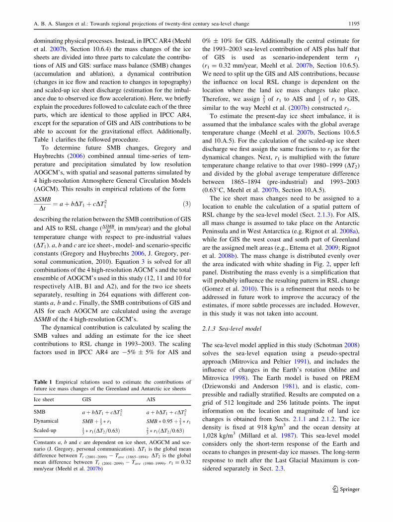
et al. 2008b). The mass change is distributed evenly over

the area indicated with white shading in Fig. 2, upper left

panel. Distributing the mass evenly is a simplification that

will probably influence the resulting pattern in RSL change

(Gomez et al. 2010). This is a refinement that needs to be

addressed in future work to improve the accuracy of the

estimates, if more subtle processes are included. However,

in this study it was not taken into account.

2.1.3 Sea-level model

The sea-level model applied in this study (Schotman 2008)

solves the sea-level equation using a pseudo-spectral

approach (Mitrovica and Peltier 1991), and includes the

influence of changes in the Earth’s rotation (Milne and

Mitrovica 1998). The Earth model is based on PREM

(Dziewonski and Anderson 1981), and is elastic, com-

pressible and radially stratified. Results are computed on a

grid of 512 longitude and 256 latitude points. The input

information on the location and magnitude of land ice

changes is obtained from Sects. 2.1.1 and 2.1.2. The ice

density is fixed at 918 kg/m3 and the ocean density at

1,028 kg/m3 (Millard et al. 1987). This sea-level model

considers only the short-term response of the Earth and

oceans to changes in present-day ice masses. The long-term

response to melt after the Last Glacial Maximum is con-

sidered separately in Sect. 2.3.

Table 1 Empirical relations used to estimate the contributions of

future ice mass changes of the Greenland and Antarctic ice sheets

Ice sheet GIS AIS

SMB aþ bDT1 þ cDT21 aþ bDT1 þ cDT2

1

Dynamical SMBþ 13� r1 SMB � 0:95þ 2

3� r1

Scaled-up 13� r1ðDT2=0:63Þ 2

3� r1ðDT2=0:63Þ

Constants a, b and c are dependent on ice sheet, AOGCM and sce-

nario (J. Gregory, personal communication). DT1 is the global mean

difference between Tt (2001–2099) - Tave (1865–1894). DT2 is the global

mean difference between Tt (2001–2099) - Tave (1980–1999). r1 = 0.32

mm/year (Meehl et al. 2007b)


123

2.2 Steric contribution

Global mean steric RSL changes are dominated by the

thermosteric part (e.g., Cazenave et al. 2009; Willis et al.

2008), since the global mean ocean salinity hardly changes

over time. Therefore, it suffices to only take into account

the global mean thermal expansion projected by the

AOGCM’s over the considered time period when calcu-

lating the steric part of the local RSL projection. Time

series of global mean thermal expansion were obtained

from the CMIP3 database (Meehl et al. 2007a) and have

been presented in IPCC AR4 (Figure 10.31). They were

corrected for model drift by subtracting the nearly linear

trend found in the accompanying preindustrial control run.

To this global mean component, we add the local RSL

anomalies projected by the AOGCM’s associated with cir-

culation changes due to temperature and salinity variations

[which are also available from the CMIP3 database, Meehl

et al. (2007a)]. By construction, the global mean of the sea-

level anomaly field is zero. These local RSL anomalies dis-

play large natural variability on interdecadal timescales. To

filter out these slow variations, we first calculate the linear

regression of local sea level over the twenty-first century at

each grid point before calculating the local RSL anomalies.

2.3 Glacial isostatic adjustment (GIA)

During the last glacial maximum, some 20,000 years ago,

large parts of the Northern hemisphere were covered by

ice. The loading of the ice caused a redistribution of

internal mass and deformation of the Earth’s surface. When

the ice started melting, the Earth did not immediately

return to its original shape, because of the delayed response

of the viscoelastic mantle. In fact, the Earth is still

adjusting today, with maximum uplift rates of around 1 cm

per year to be found in the Gulf of Bothnia and Hudson bay

(e.g. Vermeersen and Sabadini 1999). In contrast to the

influence of present-day melt of glaciers and ice sheets on

RSL change (described in Sect. 2.1), which can be com-

puted by modelling the elastic response of the Earth, the

melt of Pleistocene ice sheets has to be computed by

modelling its viscoelastic response. GIA models are mod-

els of the whole glacial cycle, mainly constrained by sea-

level information found in for instance corals and sediment

cores. Unless mentioned otherwise, we use the present-day

GIA resulting from ICE-5G(VM2) (Peltier 2004). In Sect.

4.1 we will use the ANU model (Nakada and Lambeck

1988, updated in 2004–2005), to illustrate the sensitivity of

our results to the choice of GIA model. For the time scale

of this study, the RSL changes due to GIA are almost

constant; therefore, they are applied as a stationary spatial

pattern.

2.4 Model ensemble

The RSL estimates described in this paper are calculated

using the results of simulations with the AOGCM’s given

in Table 2. These models are a subset of the World Climate

Fig. 2 Ensemble mean RSL contribution (m) of ice sheets (upper left), glaciers (upper right), steric changes (lower left) and GIA (lower right)for scenario A1B between 1980–1999 and 2090–2099. White shading in upper left panel indicates the mass loss regions on AIS and GIS


123

Research Programme’s CMIP3 multi-model dataset (Meehl

et al. 2007a) used for IPCC AR4. This subset contains all

models for which all required variables were available. For

the selected models we consider three different emission

scenarios: B1, A1B and A2, which are defined in the IPCC

Special Report on Emission Scenarios (Nakicenovic and

Swart 2000). The ensemble mean global average temper-

ature increase in 2090–2099 w.r.t. 1980–1999 is þ1:8�C(1.1–2:9�C) for B1, þ2:8�C (1.7–4:4�C) for A1B, and

þ3:4�C (2.0–5:4�C) for A2 (Meehl et al. 2007b).

The period over which we consider local RSL change is

the same as in IPCC AR4 (Table 10.7): the difference

between 1980–1999 and 2090–2099. For this period, we

extract atmospheric temperature, precipitation, the global

mean thermal expansion and the local RSL anomalies due

to temperature and salinity changes from the model data-

base (Meehl et al. 2007a). For the ice sheets (Sect. 2.1.2)

we need additional information on the global average

temperature of the pre-industrial climate (defined as the

period 1865–1894), taken from the twentieth century ref-

erence runs.

As the resolution of the different models is highly

variable, the data need to be interpolated to one grid to be

able to construct an ensemble mean. We choose a grid with

512 longitude points and 256 latitude points, as this is the

output grid of the sea-level model used to model RSL

change resulting from the land ice contributions (Sect.

2.1.3).

The size of the surface area of the ocean is model

dependent. However, if a grid point is assigned to land in

one model and to ocean in another, this complicates

comparisons between models, and especially the calcula-

tion of an ensemble mean. Therefore, in this study, RSL

change for the ensemble mean is calculated using a uni-

versal land-ocean mask which contains ocean surface area

only at those grid points where all the models have ocean

points. Use of the universal mask reduces the total ocean

surface area with respect to the model-specific masks,

leading to minor deviations in total RSL change in the

order of 2%.

3 Projections of local RSL change

3.1 Global mean projections

In Table 3 the global mean values calculated in this study

are compared to the results presented in Meehl et al.

(2007b, Table 10.7), for the emission scenario A1B. The

table shows that the results in this study are in line with

IPCC AR4, but also that there are a few differences. Firstly,

a different ensemble of AOGCM’s is used for the calcu-

lations, which influences the spread in the results of all

contributions, except GIA. Secondly, a different glacier

data set was used because locations of land ice melt were

needed to calculate the regional glacier contribution. Also,

GIA was added in this study, which is a small effect

globally averaged, but can be large locally. The last dif-

ference is that the scaled-up ice sheet discharge is separated

for the two ice sheets in this study.

Table 4 lists the global mean values for the three

emission scenarios of all the modelled RSL contributions

and the resulting total RSL change, obtained using the

methodology described in Sect. 2. The uncertainties pre-

sented in the table represent one standard deviation within

the model ensemble. Not surprisingly, the scenario with the

lowest greenhouse gas emissions, B1 (11-model ensemble),

predicts the lowest RSL rise, while the high emission A2

scenario (10-model ensemble) yields the highest estimates.

Table 4 shows that the global average GIA is slightly

positive, but very small. As GIA is a long-term effect, it is

not influenced by present-day changes, and is therefore the

same for all scenarios. The glaciers contribute a global

mean volume change of 0.17 ± 0.04 m SLE for A1B,

which is the dominant part of the land ice contribution.

Using the IPCC AR4 approach, we find that the ice sheets

(now including the estimate for the scaled-up ice sheet

discharge) contribute 0.01 ± 0.02 m from Antarctica and

0.08 ± 0.02 m from Greenland. The low value of Ant-

arctica follows from a near cancellation between the

negative SMB contribution and the positive value for the

scaled-up ice sheet discharge. Recent literature (e.g. Rignot

et al. 2008a, b, 2011; Velicogna 2009) challenges these

estimates, as current observations of the mass loss on the

ice sheets indicate that this contribution might be larger.

Table 2 CMIP3-models used in this study

AOGCM Reference

BCCR-BCM2.0 Furevik et al. (2003)

CGCM3.1(T47) Flato (2005)

ECHAM5/MPI-OM Jungclaus et al. (2006)

GFDL-CM2.0 Delworth et al. (2006)

GFDL-CM2.1 Delworth et al. (2006)

GISS-EH* Schmidt et al. (2006)

GISS-ER Schmidt et al. (2006)

GISS-AOM? Lucarini and Russell (2002)

MRI-CGCM2.3.2 Yukimoto and Noda (2002)

MIROC3.2(hires) K-1 Model Developers (2004)

NCAR-PCM Washington et al. (2000)

UKMO-HadCM3 Gordon et al. (2000)

* Not available for A2 and B1? Not available for A2


123

We will elaborate on this topic in the discussion section

(Sect. 4.1), where the influence of a larger ice sheet con-

tribution is demonstrated. However, here we will continue

to use the IPCC AR4 ice sheet estimates, including the

scaled-up ice sheet discharge, to allow for a comparison of

the regional patterns to the IPCC AR4 global mean values.

Although significantly less ice is stored in glaciers than in

the GIS and the AIS, glacier melt still provides a relatively

large contribution to RSL change. This is caused by the

higher sensitivity of glaciers to climate change due to their

larger mass turnover. The steric contribution has values

similar to the total land ice contribution, so each accounts for

about 50% of the global mean RSL change. This implies that

the total spatial pattern will depend on the steric as well as the

land ice contribution, as will be shown in Sect. 3.3.

3.2 Spatial patterns of the different contributions

The regional patterns of the separate contributions for

scenario A1B are shown in Fig. 2. We focus on this

emission scenario from now on, because it has the largest

available ensemble. Between the scenarios the amplitudes

change, but the patterns are very similar.

The upper left panel of Fig. 2 shows the RSL change

resulting from mass changes of the ice sheets. Because the

AIS contribution based on the IPCC AR4 estimates is very

small (Table 4), the pattern shown in Fig. 2 mainly results

from mass changes of the GIS. The signature of the self-

gravitation effect is clearly visible: an RSL drop close to

the largest melt source (GIS) and an above average RSL

rise in the Southern Hemisphere. In the upper right panel,

representing the contribution of the glaciers, the self-

gravitation effect is also clearly visible, but now for mul-

tiple melt sources. As most ice melts in the Northern

Hemisphere, RSL will rise by at least the global mean

value south of the equator, with the exception of the RSL

close to the Antarctic Peninsula and the Patagonian ice

fields, where values are lower due to local ice mass loss.

The contributions of ice sheets and glaciers combined lead

to a large range for the local RSL change of -3.96 to

0.30 m, with a global mean of 0.26 m.

The lower left panel of Fig. 2 shows the steric contribu-

tion. The pattern displays a large spatial variability. For

example, the region around Antarctica will experience less

sea-level change than the global mean, while according to

the climate models sea-level change in the Arctic Ocean will

be larger than average. The steric changes range from 0.01 to

0.48 m, with a global mean of 0.21 m. The pattern closely

resembles that shown in Figure 10.32 of Meehl et al.

(2007b) (note that in the latter the local sea-level change

relative to the global mean is shown while here the global

mean is included). This indicates that despite our smaller

model ensemble (12 AOGCMs versus 16 AOGCMs in

AR4), we do capture the general features of the steric pat-

tern. The underlying causes for these spatial variations in

steric sea-level change were discussed in Meehl et al.

(2007b, Section 10.6.2). For example, the relatively large

steric change in the Arctic Ocean is attributed to ocean

freshening, while the minimum found in the Southern Ocean

is due to changes in wind stress (Landerer et al. 2007) or

small thermal expansion (Lowe and Gregory 2006).

Table 3 Projected global average of RSL change (m) for SRES scenario A1B between 1980–1999 and 2090–2099, comparing this study to

IPCC AR4 estimates (their Table 10.7)

This study IPCC AR4 Remarks

Steric 0.14–0.30 0.13–0.32 Different model ensemble (this study 12, IPCC AR4 16)

Glaciers 0.13–0.25 0.08–0.15 Regionally distributed data set in this study

AIS -0.08–-0.01 -0.12–-0.02

GIS 0.04–0.08 0.01–0.08

GIA -0.001–0.009 – Not computed in IPCC AR4

Sum 0.30–0.55 0.21–0.48

Scaled-up AIS 0.04–0.06 – AIS and GIS combined in IPCC AR4: -0.01–0.13

Scaled-up GIS 0.02–0.03 –

The range given is 5–95%

Table 4 Projected ensemble mean global average of RSL change

(m) for SRES scenarios B1 (low), A1B (middle) and A2 (high)

between 1980–1999 and 2090–2099

B1 A1B A2

Steric 0.16 ± 0.08 0.21 ± 0.09 0.27 ± 0.17

Glaciers 0.14 ± 0.03 0.17 ± 0.04 0.19 ± 0.04

AIS 0.01 ± 0.02 0.01 ± 0.02 0.01 ± 0.03

GIS 0.06 ± 0.01 0.08 ± 0.02 0.08 ± 0.02

GIA 0.004 ± 0.003 0.004 ± 0.003 0.004 ± 0.003

Sum 0.37 ± 0.09 0.47 ± 0.11 0.55 ± 0.17

The sum includes the steric contribution, all land ice (including

scaled-up ice sheet discharge) and GIA. Contrarily to Table 3, the

uncertainties here are 1r between 11 models (B1), 12 models (A1B)

and 10 models (A2)


123

As GIA (Fig. 2, lower right panel) is resulting from melt

of the Laurentide and Fennoscandian ice sheets, the largest

rates of crustal deformation due to GIA can be found in

North America and Scandinavia. Changes are largest over

land, but also the sea level is influenced: RSL change

values range from -0.73 to 0.59 m, with a global mean of

0.004 m. While on average GIA is a small effect, in and

near the regions previously covered by land ice the effect

can still be quite large, and sometimes even dominate the

other contributions (e.g. Scandinavia).

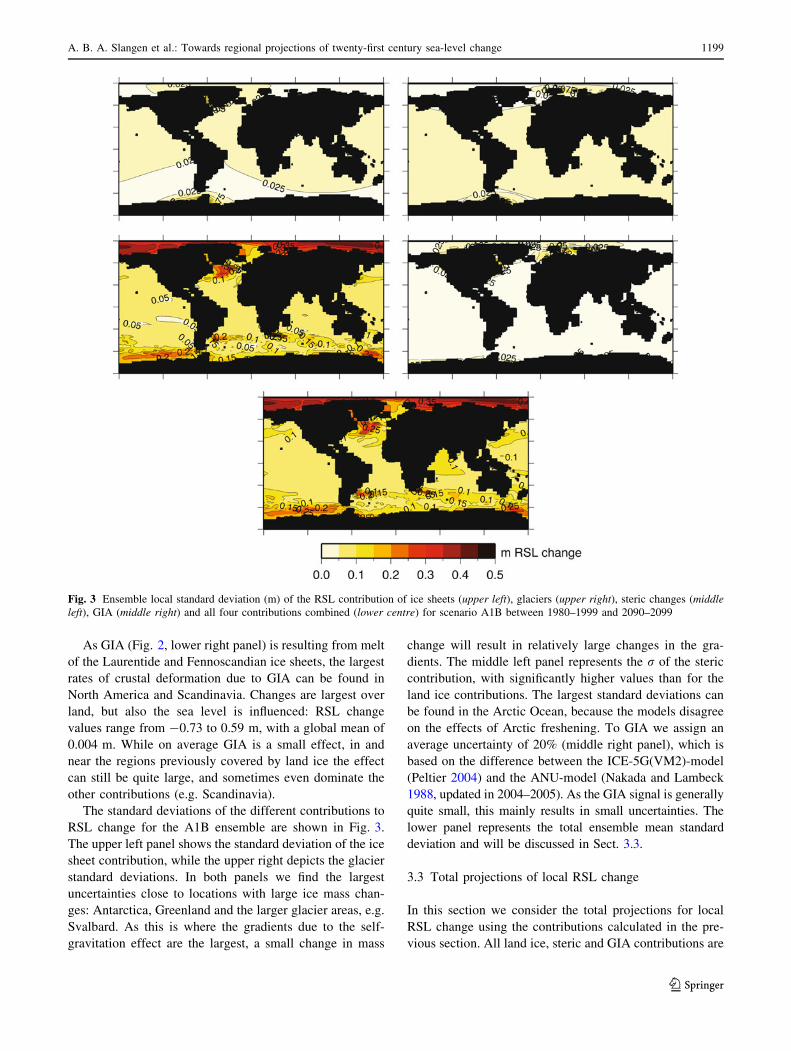
The standard deviations of the different contributions to

RSL change for the A1B ensemble are shown in Fig. 3.

The upper left panel shows the standard deviation of the ice

sheet contribution, while the upper right depicts the glacier

standard deviations. In both panels we find the largest

uncertainties close to locations with large ice mass chan-

ges: Antarctica, Greenland and the larger glacier areas, e.g.

Svalbard. As this is where the gradients due to the self-

gravitation effect are the largest, a small change in mass

change will result in relatively large changes in the gra-

dients. The middle left panel represents the r of the steric

contribution, with significantly higher values than for the

land ice contributions. The largest standard deviations can

be found in the Arctic Ocean, because the models disagree

on the effects of Arctic freshening. To GIA we assign an

average uncertainty of 20% (middle right panel), which is

based on the difference between the ICE-5G(VM2)-model

(Peltier 2004) and the ANU-model (Nakada and Lambeck

1988, updated in 2004–2005). As the GIA signal is generally

quite small, this mainly results in small uncertainties. The

lower panel represents the total ensemble mean standard

deviation and will be discussed in Sect. 3.3.

3.3 Total projections of local RSL change

In this section we consider the total projections for local

RSL change using the contributions calculated in the pre-

vious section. All land ice, steric and GIA contributions are

Fig. 3 Ensemble local standard deviation (m) of the RSL contribution of ice sheets (upper left), glaciers (upper right), steric changes (middleleft), GIA (middle right) and all four contributions combined (lower centre) for scenario A1B between 1980–1999 and 2090–2099


123

added together, and the result is shown in Fig. 4 for the

three scenarios: A1B (upper panel), B1 (middle panel) and

A2 (lower panel). While the global mean differs (Table 4),

all scenarios show a similarly large spatial variability, with

no significant differences in the spatial pattern. In all three

panels, the spatial variability in the steric contribution has a

large impact on the ensemble mean pattern. We observe for

instance in all scenarios a band of relative high RSL rise

stretching from South America into the Indian Ocean.

However, looking closer reveals influences of the other

contributions too. The effect of Arctic freshening is less

pronounced, because the steric contribution is partly bal-

anced by the other contributions. We observe the influence

of GIA for instance between Iceland and Scandinavia: the

RSL change is large since this region lies on the peripheral

bulge (Peltier 2004) and thus the Earth’s surface is

lowering here. Also future land ice melt influences the

pattern, for instance in the Arctic Ocean, where it coun-

teracts the influence of the steric changes, and around the

Antarctic Peninsula, where a sea-level drop is projected as

a result of the self-gravitation effect.

The total ensemble mean standard deviation of scenario

A1B is shown in the lower panel of Fig. 3. Here we see that

the total uncertainty, when adopting the IPCC AR4

approach for the ice sheets, is dominated by uncertainties

in the steric contribution, since the values of the standard

deviations of land ice and GIA are significantly smaller.

Hence, the largest standard deviations can be found in the

Arctic Ocean and the Southern Ocean.

Figure 5 shows how much the projection for the local

sea level deviates from the ensemble mean global mean

value for scenario A1B. The figure emphasizes the large

spatial variability of RSL change, as it shows that the local

values rarely equal the global mean value. Some regions

experience a notably lower RSL, while others have extre-

mely large RSL rise compared to the global mean, with a

pattern that is qualitatively similar for all scenarios (not

shown).

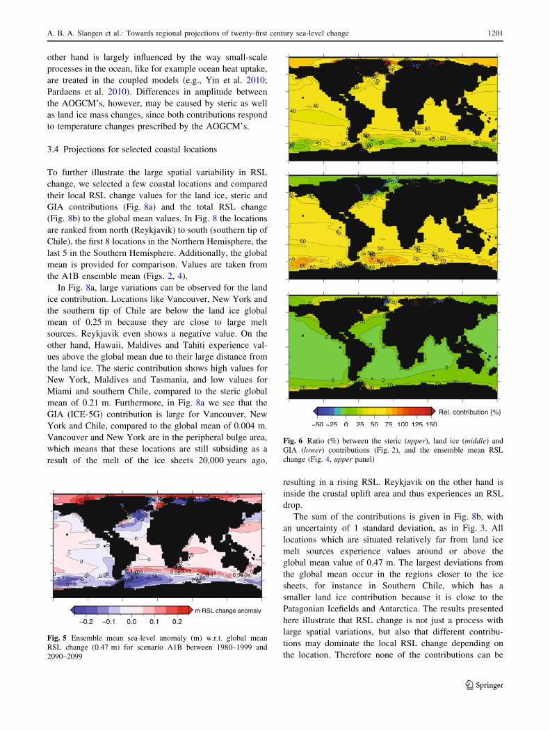
In order to examine the influence of the different con-

tributions on the total projected RSL change and the spatial

pattern, we show maps of the individual contributions as a

fraction of the total value for A1B in Fig. 6. The upper

panel shows the ratio of the steric contribution, the middle

panel the land ice ratio and the lower panel the GIA ratio,

all relative to the total projection. There is a large region

around the equator which shows very little influence of

GIA and a 50–50% contribution for land ice and steric

contributions. In the Arctic Ocean, the steric contribution is

slightly larger due to Arctic freshening, which is enhanced

by GIA but balanced by a relatively low contribution of

land ice mass loss. Around Antarctica there is a large band

where the steric contribution has relatively little influence

(10–30%), and land ice mass loss for a large part explains

future RSL change in that region (60–80%).

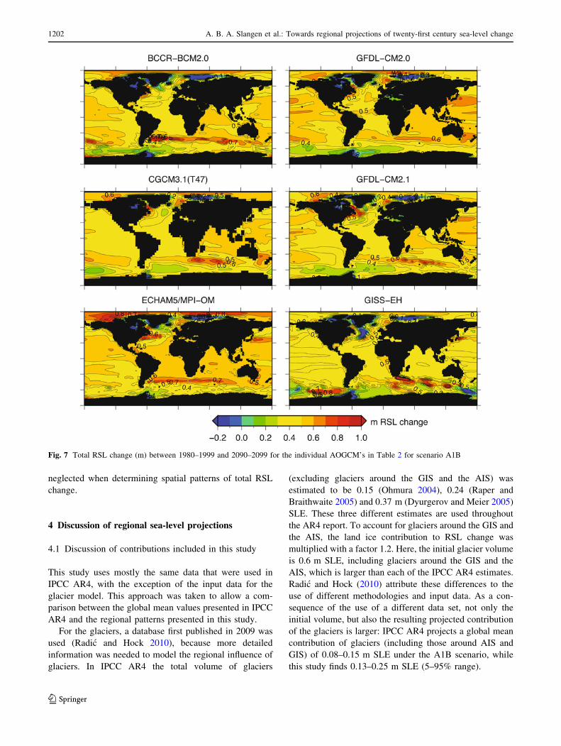
The ensemble mean total projection of A1B is an

average of 12 AOGCM’s. The total projected RSL change

for each AOGCM (for A1B) with their model-specific

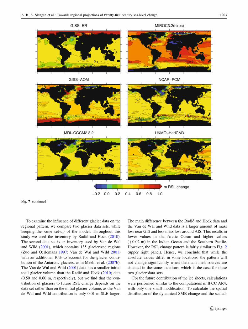
land-sea mask, is shown in Fig. 7. Most AOGCM’s show a

pattern fairly similar to the ensemble mean, with slightly

more spatial variation, which is smoothed in the ensemble

mean. However, some models show overall higher values

for RSL change [MIROC3.2(hires)], while others are

below the ensemble mean (NCAR-PCM and MRI-

CGCM2.3.2). The differences in spatial patterns between

the models arise mainly from the steric component,

because the land ice contribution pattern is fairly similar

for all AOGCM’s as the amount of ice melt may vary

depending on the temperature and precipitation change, but

the locations do not change. The steric component on the

Fig. 4 Ensemble mean total RSL change (m) between 1980–1999

and 2090–2099 for scenario A1B (upper based on 12 models), B1

(middle based on 11 models) and A2 (lower based on 10 models)


123

other hand is largely influenced by the way small-scale

processes in the ocean, like for example ocean heat uptake,

are treated in the coupled models (e.g., Yin et al. 2010;

Pardaens et al. 2010). Differences in amplitude between

the AOGCM’s, however, may be caused by steric as well

as land ice mass changes, since both contributions respond

to temperature changes prescribed by the AOGCM’s.

3.4 Projections for selected coastal locations

To further illustrate the large spatial variability in RSL

change, we selected a few coastal locations and compared

their local RSL change values for the land ice, steric and

GIA contributions (Fig. 8a) and the total RSL change

(Fig. 8b) to the global mean values. In Fig. 8 the locations

are ranked from north (Reykjavik) to south (southern tip of

Chile), the first 8 locations in the Northern Hemisphere, the

last 5 in the Southern Hemisphere. Additionally, the global

mean is provided for comparison. Values are taken from

the A1B ensemble mean (Figs. 2, 4).

In Fig. 8a, large variations can be observed for the land

ice contribution. Locations like Vancouver, New York and

the southern tip of Chile are below the land ice global

mean of 0.25 m because they are close to large melt

sources. Reykjavik even shows a negative value. On the

other hand, Hawaii, Maldives and Tahiti experience val-

ues above the global mean due to their large distance from

the land ice. The steric contribution shows high values for

New York, Maldives and Tasmania, and low values for

Miami and southern Chile, compared to the steric global

mean of 0.21 m. Furthermore, in Fig. 8a we see that the

GIA (ICE-5G) contribution is large for Vancouver, New

York and Chile, compared to the global mean of 0.004 m.

Vancouver and New York are in the peripheral bulge area,

which means that these locations are still subsiding as a

result of the melt of the ice sheets 20,000 years ago,

resulting in a rising RSL. Reykjavik on the other hand is

inside the crustal uplift area and thus experiences an RSL

drop.

The sum of the contributions is given in Fig. 8b, with

an uncertainty of 1 standard deviation, as in Fig. 3. All

locations which are situated relatively far from land ice

melt sources experience values around or above the

global mean value of 0.47 m. The largest deviations from

the global mean occur in the regions closer to the ice

sheets, for instance in Southern Chile, which has a

smaller land ice contribution because it is close to the

Patagonian Icefields and Antarctica. The results presented

here illustrate that RSL change is not just a process with

large spatial variations, but also that different contribu-

tions may dominate the local RSL change depending on

the location. Therefore none of the contributions can be

Fig. 5 Ensemble mean sea-level anomaly (m) w.r.t. global mean

RSL change (0.47 m) for scenario A1B between 1980–1999 and

2090–2099

Fig. 6 Ratio (%) between the steric (upper), land ice (middle) and

GIA (lower) contributions (Fig. 2), and the ensemble mean RSL

change (Fig. 4, upper panel)


123

neglected when determining spatial patterns of total RSL

change.

4 Discussion of regional sea-level projections

4.1 Discussion of contributions included in this study

This study uses mostly the same data that were used in

IPCC AR4, with the exception of the input data for the

glacier model. This approach was taken to allow a com-

parison between the global mean values presented in IPCC

AR4 and the regional patterns presented in this study.

For the glaciers, a database first published in 2009 was

used (Radic and Hock 2010), because more detailed

information was needed to model the regional influence of

glaciers. In IPCC AR4 the total volume of glaciers

(excluding glaciers around the GIS and the AIS) was

estimated to be 0.15 (Ohmura 2004), 0.24 (Raper and

Braithwaite 2005) and 0.37 m (Dyurgerov and Meier 2005)

SLE. These three different estimates are used throughout

the AR4 report. To account for glaciers around the GIS and

the AIS, the land ice contribution to RSL change was

multiplied with a factor 1.2. Here, the initial glacier volume

is 0.6 m SLE, including glaciers around the GIS and the

AIS, which is larger than each of the IPCC AR4 estimates.

Radic and Hock (2010) attribute these differences to the

use of different methodologies and input data. As a con-

sequence of the use of a different data set, not only the

initial volume, but also the resulting projected contribution

of the glaciers is larger: IPCC AR4 projects a global mean

contribution of glaciers (including those around AIS and

GIS) of 0.08–0.15 m SLE under the A1B scenario, while

this study finds 0.13–0.25 m SLE (5–95% range).

Fig. 7 Total RSL change (m) between 1980–1999 and 2090–2099 for the individual AOGCM’s in Table 2 for scenario A1B


123

To examine the influence of different glacier data on the

regional pattern, we compare two glacier data sets, while

keeping the same set-up of the model. Throughout this

study we used the inventory by Radic and Hock (2010).

The second data set is an inventory used by Van de Wal

and Wild (2001), which contains 135 glacierized regions

(Zuo and Oerlemans 1997; Van de Wal and Wild 2001)

with an additional 10% to account for the glacier contri-

bution of the Antarctic glaciers, as in Meehl et al. (2007b).

The Van de Wal and Wild (2001) data has a smaller initial

total glacier volume than the Radic and Hock (2010) data

(0.50 and 0.60 m, respectively), but we find that the con-

tribution of glaciers to future RSL change depends on the

data set rather than on the initial glacier volume, as the Van

de Wal and Wild-contribution is only 0.01 m SLE larger.

The main difference between the Radic and Hock data and

the Van de Wal and Wild data is a larger amount of mass

loss near GIS and less mass loss around AIS. This results in

lower values in the Arctic Ocean and higher values

(?0.02 m) in the Indian Ocean and the Southern Pacific.

However, the RSL change pattern is fairly similar to Fig. 2

(upper right panel). Hence, we conclude that while the

absolute values differ in some locations, the pattern will

not change significantly when the main melt sources are

situated in the same locations, which is the case for these

two glacier data sets.

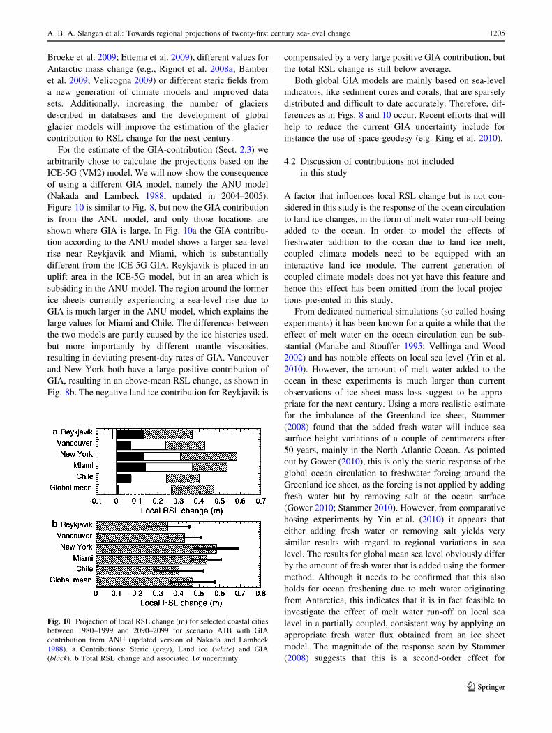
For the future contribution of the ice sheets, calculations

were performed similar to the computations in IPCC AR4,

with only one small modification. To calculate the spatial

distribution of the dynamical SMB change and the scaled-

Fig. 7 continued


123

up ice sheet discharge, the contributions needed to be

calculated separately for each ice sheet, instead of using

one value for both ice sheets combined, as in the IPCC

AR4 report.

Although the results reported in IPCC AR4 were the

state of the art on climate change in 2007, recent research

has updated the estimates and models of different aspects

regarding climate change. Nevertheless, we deliberately

chose to stay as close as possible to the AR4 report in order

to allow for a comparison of the spatial patterns to the well-

known IPCC AR4 global mean values. To illustrate how

this choice influences the results, we recalculated the RSL

change with larger estimates for the contributions of the ice

sheets, as recent observations show a faster increase in

mass loss than estimated in IPCC AR4 (e.g., Rignot et al.

2008a, b, 2011; Velicogna 2009). For this example, we use

a high-end estimate of 0.41 m SLE for the AIS and 0.22 m

SLE for the GIS, as suggested by Katsman et al. (2010)

based on a reassessment of the dynamical contribution of

the ice sheets considering recent observations and expert

judgement. Contrarily to the calculations done in Sect. 3,

the ice sheet contribution is now fixed and thus not

dependent on the temperature and precipitation provided

by the climate models. This means that an ensemble spread

could not be calculated for this experiment. However, as

the contribution of the ice sheets is much larger than in

Sect. 3, it will probably show larger variations for differ-

ences in climate, which would lead to a larger spread than

displayed in Fig. 3, but it is uncertain how much this would

differ exactly. All the other contributions are the same as

presented in Table 4 and Fig. 2, the A1B scenario. Adding

all the contributions now leads to a global mean RSL

change of 1.02 m SLE. The resulting anomaly with respect

to the ensemble global mean RSL change is shown in

Fig. 9. The ice sheets now account for 60% of the total

RSL change instead of only 25% in the IPCC AR4. This

clearly influences the pattern in Fig. 9, compared to Fig. 5.

The large amount of land ice melt on both ice sheets causes

large sea-level drop regions around them. Also, the RSL

rise around the equator is much larger due to the self-

gravitation effect. These effects are also shown in e.g.

Bamber and Riva (2010) and Riva et al. (2010) and are a

direct consequence of the gravitational attraction. The

steric contribution now only accounts for 20% of the global

mean instead of 45%, which means that the land ice melt is

the dominant contribution. Still, features of the steric

component and the GIA remain present, but less

pronounced.

The example shown in Fig. 9 illustrates the importance

of using the best estimates possible when calculating

regional RSL variations, as the total pattern in RSL change

depends on the pattern from each of the contributions.

Therefore, in the future, our model strategy can easily be

used with better estimations for Greenland mass change

(e.g., Fettweis et al. 2008; Rignot et al. 2008b; Van den

Fig. 8 Projection of local RSL change (m) for selected coastal cities

between 1980–1999 and 2090–2099 for scenario A1B. a Contribu-

tions: Steric (grey), Land ice (white) and GIA (black). b Total RSL

change and associated 1r uncertainty

Fig. 9 Ensemble mean sea-level anomaly (m) w.r.t. global mean

RSL change (1.02 m) for scenario A1B between 1980–1999 and

2090–2099, for a scenario with adapted ice sheet contributions of

0.22 m for GIS and 0.41 m for AIS


123

Broeke et al. 2009; Ettema et al. 2009), different values for

Antarctic mass change (e.g., Rignot et al. 2008a; Bamber

et al. 2009; Velicogna 2009) or different steric fields from

a new generation of climate models and improved data

sets. Additionally, increasing the number of glaciers

described in databases and the development of global

glacier models will improve the estimation of the glacier

contribution to RSL change for the next century.

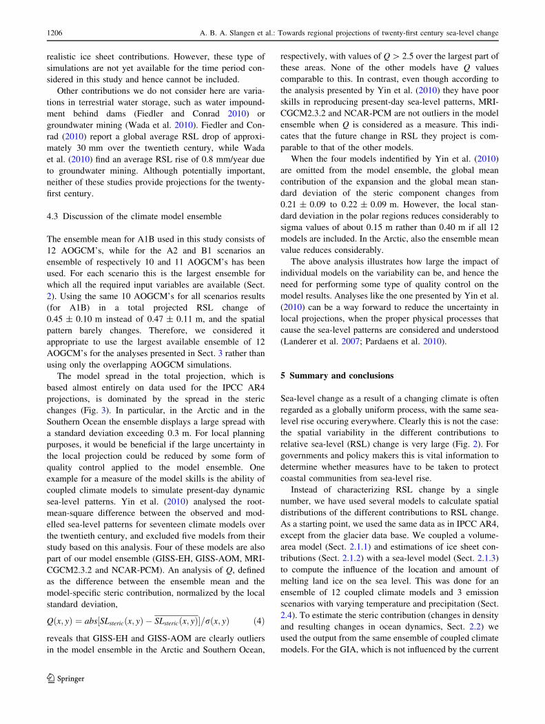
For the estimate of the GIA-contribution (Sect. 2.3) we

arbitrarily chose to calculate the projections based on the

ICE-5G (VM2) model. We will now show the consequence

of using a different GIA model, namely the ANU model

(Nakada and Lambeck 1988, updated in 2004–2005).

Figure 10 is similar to Fig. 8, but now the GIA contribution

is from the ANU model, and only those locations are

shown where GIA is large. In Fig. 10a the GIA contribu-

tion according to the ANU model shows a larger sea-level

rise near Reykjavik and Miami, which is substantially

different from the ICE-5G GIA. Reykjavik is placed in an

uplift area in the ICE-5G model, but in an area which is

subsiding in the ANU-model. The region around the former

ice sheets currently experiencing a sea-level rise due to

GIA is much larger in the ANU-model, which explains the

large values for Miami and Chile. The differences between

the two models are partly caused by the ice histories used,

but more importantly by different mantle viscosities,

resulting in deviating present-day rates of GIA. Vancouver

and New York both have a large positive contribution of

GIA, resulting in an above-mean RSL change, as shown in

Fig. 8b. The negative land ice contribution for Reykjavik is

compensated by a very large positive GIA contribution, but

the total RSL change is still below average.

Both global GIA models are mainly based on sea-level

indicators, like sediment cores and corals, that are sparsely

distributed and difficult to date accurately. Therefore, dif-

ferences as in Figs. 8 and 10 occur. Recent efforts that will

help to reduce the current GIA uncertainty include for

instance the use of space-geodesy (e.g. King et al. 2010).

4.2 Discussion of contributions not included

in this study

A factor that influences local RSL change but is not con-

sidered in this study is the response of the ocean circulation

to land ice changes, in the form of melt water run-off being

added to the ocean. In order to model the effects of

freshwater addition to the ocean due to land ice melt,

coupled climate models need to be equipped with an

interactive land ice module. The current generation of

coupled climate models does not yet have this feature and

hence this effect has been omitted from the local projec-

tions presented in this study.

From dedicated numerical simulations (so-called hosing

experiments) it has been known for a quite a while that the

effect of melt water on the ocean circulation can be sub-

stantial (Manabe and Stouffer 1995; Vellinga and Wood

2002) and has notable effects on local sea level (Yin et al.

2010). However, the amount of melt water added to the

ocean in these experiments is much larger than current

observations of ice sheet mass loss suggest to be appro-

priate for the next century. Using a more realistic estimate

for the imbalance of the Greenland ice sheet, Stammer

(2008) found that the added fresh water will induce sea

surface height variations of a couple of centimeters after

50 years, mainly in the North Atlantic Ocean. As pointed

out by Gower (2010), this is only the steric response of the

global ocean circulation to freshwater forcing around the

Greenland ice sheet, as the forcing is not applied by adding

fresh water but by removing salt at the ocean surface

(Gower 2010; Stammer 2010). However, from comparative

hosing experiments by Yin et al. (2010) it appears that

either adding fresh water or removing salt yields very

similar results with regard to regional variations in sea

level. The results for global mean sea level obviously differ

by the amount of fresh water that is added using the former

method. Although it needs to be confirmed that this also

holds for ocean freshening due to melt water originating

from Antarctica, this indicates that it is in fact feasible to

investigate the effect of melt water run-off on local sea

level in a partially coupled, consistent way by applying an

appropriate fresh water flux obtained from an ice sheet

model. The magnitude of the response seen by Stammer

(2008) suggests that this is a second-order effect for

Fig. 10 Projection of local RSL change (m) for selected coastal cities

between 1980–1999 and 2090–2099 for scenario A1B with GIA

contribution from ANU (updated version of Nakada and Lambeck

1988). a Contributions: Steric (grey), Land ice (white) and GIA

(black). b Total RSL change and associated 1r uncertainty


123

realistic ice sheet contributions. However, these type of

simulations are not yet available for the time period con-

sidered in this study and hence cannot be included.

Other contributions we do not consider here are varia-

tions in terrestrial water storage, such as water impound-

ment behind dams (Fiedler and Conrad 2010) or

groundwater mining (Wada et al. 2010). Fiedler and Con-

rad (2010) report a global average RSL drop of approxi-

mately 30 mm over the twentieth century, while Wada

et al. (2010) find an average RSL rise of 0.8 mm/year due

to groundwater mining. Although potentially important,

neither of these studies provide projections for the twenty-

first century.

4.3 Discussion of the climate model ensemble

The ensemble mean for A1B used in this study consists of

12 AOGCM’s, while for the A2 and B1 scenarios an

ensemble of respectively 10 and 11 AOGCM’s has been

used. For each scenario this is the largest ensemble for

which all the required input variables are available (Sect.

2). Using the same 10 AOGCM’s for all scenarios results

(for A1B) in a total projected RSL change of

0.45 ± 0.10 m instead of 0.47 ± 0.11 m, and the spatial

pattern barely changes. Therefore, we considered it

appropriate to use the largest available ensemble of 12

AOGCM’s for the analyses presented in Sect. 3 rather than

using only the overlapping AOGCM simulations.

The model spread in the total projection, which is

based almost entirely on data used for the IPCC AR4

projections, is dominated by the spread in the steric

changes (Fig. 3). In particular, in the Arctic and in the

Southern Ocean the ensemble displays a large spread with

a standard deviation exceeding 0.3 m. For local planning

purposes, it would be beneficial if the large uncertainty in

the local projection could be reduced by some form of

quality control applied to the model ensemble. One

example for a measure of the model skills is the ability of

coupled climate models to simulate present-day dynamic

sea-level patterns. Yin et al. (2010) analysed the root-

mean-square difference between the observed and mod-

elled sea-level patterns for seventeen climate models over

the twentieth century, and excluded five models from their

study based on this analysis. Four of these models are also

part of our model ensemble (GISS-EH, GISS-AOM, MRI-

CGCM2.3.2 and NCAR-PCM). An analysis of Q, defined

as the difference between the ensemble mean and the

model-specific steric contribution, normalized by the local

standard deviation,

Qðx; yÞ ¼ abs½SLstericðx; yÞ � SLstericðx; yÞ�=rðx; yÞ ð4Þ

reveals that GISS-EH and GISS-AOM are clearly outliers

in the model ensemble in the Arctic and Southern Ocean,

respectively, with values of Q [ 2.5 over the largest part of

these areas. None of the other models have Q values

comparable to this. In contrast, even though according to

the analysis presented by Yin et al. (2010) they have poor

skills in reproducing present-day sea-level patterns, MRI-

CGCM2.3.2 and NCAR-PCM are not outliers in the model

ensemble when Q is considered as a measure. This indi-

cates that the future change in RSL they project is com-

parable to that of the other models.

When the four models indentified by Yin et al. (2010)

are omitted from the model ensemble, the global mean

contribution of the expansion and the global mean stan-

dard deviation of the steric component changes from

0.21 ± 0.09 to 0.22 ± 0.09 m. However, the local stan-

dard deviation in the polar regions reduces considerably to

sigma values of about 0.15 m rather than 0.40 m if all 12

models are included. In the Arctic, also the ensemble mean

value reduces considerably.

The above analysis illustrates how large the impact of

individual models on the variability can be, and hence the

need for performing some type of quality control on the

model results. Analyses like the one presented by Yin et al.

(2010) can be a way forward to reduce the uncertainty in

local projections, when the proper physical processes that

cause the sea-level patterns are considered and understood

(Landerer et al. 2007; Pardaens et al. 2010).

5 Summary and conclusions

Sea-level change as a result of a changing climate is often

regarded as a globally uniform process, with the same sea-

level rise occuring everywhere. Clearly this is not the case:

the spatial variability in the different contributions to

relative sea-level (RSL) change is very large (Fig. 2). For

governments and policy makers this is vital information to

determine whether measures have to be taken to protect

coastal communities from sea-level rise.

Instead of characterizing RSL change by a single

number, we have used several models to calculate spatial

distributions of the different contributions to RSL change.

As a starting point, we used the same data as in IPCC AR4,

except from the glacier data base. We coupled a volume-

area model (Sect. 2.1.1) and estimations of ice sheet con-

tributions (Sect. 2.1.2) with a sea-level model (Sect. 2.1.3)

to compute the influence of the location and amount of

melting land ice on the sea level. This was done for an

ensemble of 12 coupled climate models and 3 emission

scenarios with varying temperature and precipitation (Sect.

2.4). To estimate the steric contribution (changes in density

and resulting changes in ocean dynamics, Sect. 2.2) we

used the output from the same ensemble of coupled climate

models. For the GIA, which is not influenced by the current


123

climate but a result of climate change 20,000 years ago, we

used results of a glaciation-deglaciation model to estimate

the influence on RSL change (Sect. 2.3).

In most regions, the two largest contributions are the

addition of mass (the land ice component) and the changes

in density (the steric component), while GIA is only large

in some specific areas (Fig. 2). The steric component

shows very large spatial variations, because changes in

density occur when ocean currents change, fresh water is

added or atmospheric temperature changes. The land ice

contribution on the other hand also shows large variations,

but with a distinctive pattern due to elastic solid Earth

deformation and the self-gravitation effect. Globally aver-

aged, both the land ice contribution and the steric contri-

bution account individually for about 50% of the RSL

change (Table 4). However, considering the total projected

spatial pattern reveals that all contributions included in this

study, even GIA, can dominate the local RSL change,

depending on the location (Figs. 4, 8). The amplitudes of

the local RSL change differ per scenario, but the patterns

are fairly similar. The spread in the local RSL change for

the projection based on the data used in IPCC AR4 is

dominated by the spread in the steric contribution between

the different AOGCM’s, while the uncertainty in the land

ice contribution is largest close to the land ice melt source

and fairly small otherwise (Fig. 3). An increase in the

estimation of the ice sheet contribution might also increase

the spread for this contribution, but it is uncertain whether

the result will be as large as the spread in the steric

contribution.

The absolute values presented in this study should be

interpreted carefully. In Sect. 4.1 we have shown that

following the approach taken by IPCC AR4 introduces a

potential underestimation in the ice sheet contributions,

which would influence the pattern substantially (Fig. 9).

This section also discusses the choice of GIA model, which

is a small contribution when globally averaged, but can

dominate RSL change locally. Additionally, this section

shows that the projections are not very sensitive to the

choice of glacier data set.

We have shown with this study that it is possible to

model regional variability in future RSL change, by using a

combination of spatial patterns of steric effects, land ice

melt and GIA obtained from different models. Improve-

ments can be made, for instance by adding a coupling

between ice melt and ocean dynamics or by better esti-

mates for the land ice melt. Irrespective of the details in

methodology, we think that scientific understanding now

allows to discuss regional patterns rather than only the

global mean values.

Acknowledgments We would like to thank J. Gregory for provid-

ing the SMB constants and the additional expansion data, V. Radic for

help with the WGI-XF data and J. Cogley for making this dataset

available. We would also like to thank P. Stocchi and K. Lambeck for

providing us with the ANU model. We acknowledge the international

modeling groups for providing their data for analysis, the Program for

Climate Model Diagnosis and Intercomparison (PCMDI) for col-

lecting and archiving the model data, the JSC/CLIVAR Working

Group on Coupled Modelling (WGCM) and their Coupled Model

Intercomparison Project (CMIP) and Climate Simulation Panel for

organizing the model data analysis activity, and the IPCC WG1 TSU

for technical support. A.S is supported by the Netherlands Institute for

Space Research (SRON) (ALW-GO-AO/07-14). We thank two

anonymous reviewers for their useful comments.

Open Access This article is distributed under the terms of the

Creative Commons Attribution Noncommercial License which per-

mits any noncommercial use, distribution, and reproduction in any

medium, provided the original author(s) and source are credited.

References

Antonov JI, Levitus S, Boyer TP (2002) Steric sea level variations

during 1957–1994: importance of salinity. J Geophys Res

107(C12):8013. doi:10.1029/2001JC000,964

Bahr DB, Meier MF, Peckham SD (1997) The physical basis

of glacier volume-area scaling. J Geophys Res 102(B9):

20,355–20,362

Bamber J, Riva R (2010) The sea level fingerprint of recent ice mass

fluxes. Cryosphere 4:621–627. doi:10.5194/tc-4-621-2010

Bamber JL, Riva REM, Vermeersen LLA, LeBrocq AM (2009)

Reassessment of the potential sea-level rise from a collapse of

the West Antarctic ice sheet. Science 324:901–903

Bindoff NL, Willebrand J, Artale V, Cazenave A, Gregory J, Gulev S,

Hanawa K, Quere CL, Levitus S, Nojiri Y, Shum CK, Talley LD,

Unnikrishnan A (2007) Observations: oceanic climate change

and sea level. In: Solomon S, Qin D, Manning M, Chen Z,

Marquis M, Averyt KB, Tignor M, Miller HL (eds) Climate

change 2007: the physical science basis. Contribution of working

group I to the 4th assessment report of the intergovernmental

panel on climate change. Cambridge University Press,

Cambridge

Cazenave A, Nerem RS (2004) Present-day sea level change:

observations and causes. Rev Geophys 42(RG3001)

Cazenave A, Dominh K, Guinehut S, Berthier E, Llovel W, Ramilien

G, Ablain M, Larnicol G (2009) Sea level budget over

2003–2008. A reevaluation from GRACE space gravimetry,

satellite altimetry and ARGO. Glob Planet Change 65:83–88.

doi:10.1016/j.gloplacha.2008.10.004

Chen J, Ohmura A (1990) Estimation of Alpine glacier water

resources and their change since the 1870’s. IAHS 193:127–135

Cogley JG (2009) A more complete version of the World Glacier

Inventory. Ann Glaciol 50:32–38

Delworth TL, Broccoli AJ, Rosati A, Stouffer RJ, Balaji V, Beesley

JA, Cooke WF, Dixon KW, Dunne J, Dunne KA, Durachta JW,

Findell KL, Ginoux P, Gnanadesikan A, Gordon CT, Griffies

SM, Gudgel R, Harrison MJ, Held IM, Hemler RS, Horowitz

LW, Klein SA, Knutson TR, Kushner PJ, Langenhorst AR, Lee

HC, Lin SJ, Lu J, Malyshev SL, Milly PCD, Ramaswamy V,

Russell J, Schwarzkopf MD, Shevliakova E, Sirutis JJ, Spelman

MJ, Stern WF, Winton M, Wittenberg AT, Wyman B, Zeng F,

Zhang R (2006) GFDL’s CM2 global coupled climate models.

Part I: formulation and simulation characteristics. J Clim

19:643–674


123

http://dx.doi.org/10.1029/2001JC000,964

http://dx.doi.org/10.5194/tc-4-621-2010

http://dx.doi.org/10.1016/j.gloplacha.2008.10.004

Dyurgerov MB, Meier MF (2005) Glaciers and the changing earth

system: a 2004 snapshot. Tech. rep., Inst. of Arct. and Alp. Res.,

Univ. of Colo., Boulder, Occas Pap No 58

Dziewonski AM, Anderson DL (1981) Preliminary reference Earth

model. Phys Earth Planet Inter 25:297–356

Ettema J, van den Broeke MR, van Meijgaard E, van de Berg WJ,

Bamber JL, Box JE, Bales RC (2009) Higher surface mass

balance of the Greenland ice sheet revealed by high-resolution

climate modeling. Geophys Res Lett 36(12). doi: 10.1029/2009

GL038110

Farrell WE, Clark JA (1976) On postglacial sea level. Geophys J R

Astron Soc 46:647–667

Fettweis X, Hanna E, Gallee H, Huybrechts P, Erpicum M (2008)

Estimation of the Greenland ice sheet surface mass balance for

the 20th and 21st centuries. Cryosphere 2(2):117–129. doi:

10.5194/tc-2-117-2008

Fiedler JW, Conrad CP (2010) Spatial variability of sea level rise due

to water impoundment behind dams. Geophys Res Lett

37(L12603). doi:10.1029/2010GL043462

Flato GM (2005) The third generation coupled global climate model

(CGCM3). http://www.cccma.ec.gc.ca/models/cgcm3.shtml

Furevik T, Bentsen M, Drange H, Kvamsto N, Sorteberg A (2003)

Description and evaluation of the Bergen climate model:

ARPEGE coupled with MICOM. Clim Dyn 21:27–51

Gomez N, Mitrovica JX, Tamisiea ME, Clark PU (2010) A new

projection of sea level change in response to collapse of marine

sectors of the Antarctic Ice Sheet. Geophys J Int 180:623–634.

doi:10.1111/j.1365-246X.2009.04419.x

Gordon C, Cooper C, Senior CA, Banks HT, Gregory JM, Johns TC,

Mitchell JFB, Wood RA (2000) The simulation of SST, sea ice

extents and ocean heat transports in a version of the Hadley

Centre coupled model without flux adjustments. Clim Dyn

16:147–168

Gower JFR (2010) Comment on ’’Response of the global ocean to

Greenland and Antarctic ice melting’’; by D. Stammer. J Geophys

Res 115(C10009). doi:10.1029/2010JC006097

Gregory JM, Huybrechts P (2006) Ice-sheet contributions to future

sea-level change. Phil Trans R Soc A 364:1709–1731. doi:

10.1098/rsta.2006.1796

Jungclaus JH, Keenlyside N, Botzet M, Haak H, Luo JJ, Latif M,

Marotzke J, Mikolajewicz U, Roeckner E (2006) Ocean

circulation and tropical variability in the coupled model

ECHAM5/MPI-OM. J Clim 19:3952–3972

K-1 Model Developers (2004) K-1 coupled model (MIROC)

description. Tech rep 1, Center for Climate System Research,

University of Tokyo

Katsman CA, Sterl A, Beersma JJ, van den Brink HW, Church JA,

Hazeleger W, Kopp RE, Kroon D, Kwadijk J, Lammersen R,

Lowe J, Oppenheimer M, Plag H.-P., Ridley J, von Storch H,

Vaughan DG, Vellinga P, Vermeersen LLA, van de Wal RSW,

Weisse R (2010) Exploring high-end scenarios for local sea level

rise to develop flood protection strategies for a low-lying delta -

the Netherlands as an example. Clim Change (in press)

King M, Altamimi Z, Boehm J, Bos M, Dach R, Elosegui P, Fund F,

Hernandez-Pajares M, Lavallee D, Cerveira PM, Penna N, Riva

R, Steigenberger P, van Dam T, Vittuari L, Williams S, Willis P

(2010) Improved constraints to models of glacial isostatic

adjustment: a review of the contribution of ground-based

geodetic observations. Surv Geophys 31(5):465–507. doi:

10.1007/s10712-010-9100-4

Landerer FW, Jungclaus JH, Marotzke J (2007) Regional dynamic

and steric sea level change in response to the IPCC-A1B

scenario. J Phys Oceanogr 37:296–312

Lemke P, Ren J, Alley RB, Allison I, Carrasco J, Flato G, Fujii Y,

Kaser G, Mote P, Thomas RH, Zhang T (2007) Observations:

changes in snow, ice and frozen ground. In: Solomon S, Qin D,

Manning M, Chen Z, Marquis M, Averyt KB, Tignor M, Miller

HL (eds) Climate change 2007: the physical science basis.

Contribution of working group I to the 4th assessment report of

the intergovernmental panel on climate change. Cambridge

University Press, Cambridge

Lowe JA, Gregory JM (2006) Understanding projections of sea level

rise in a hadley centre coupled climate model. J Geophys Res

111(C11014). doi:10.1029/2005JC003421

Lucarini L, Russell GL (2002) Comparison of mean climate trends in

the northern hemisphere between National Centers for Environ-

mental Prediction and two atmosphere-ocean model forced runs.

J Geophys Res 107(D15):4269. doi:10.1029/2001JD001247

Manabe S, Stouffer RJ (1996) Simulation of abrupt climate change

induced by freshwater input to the North Atlantic Ocean. Nature

378:165–167. doi:10.1038/378165a0

Meehl GA, Covey C, Delworth T, Latif M, McAvaney B, Mitchell

JFB, Stouffer RJ, Taylor KE (2007) The WCRP CMIP3 multi-

model dataset: a new era in climate change research. Bull Am

Meteorol Soc 88:1383–1394

Meehl GA, Stocker TF, Collins WD, Friedlingstein P, Gaye A,

Gregory J, Kitoh A, Knutti R, Murphy J, Noda A, Raper S,

Watterson I, Weaver A, Zhao ZC (2007b) Global climate

projections. In: Solomon S, Qin D, Manning M, Chen Z, Marquis

M, Averyt KB, Tignor M, Miller HL (eds), Climate change

2007: the physical science basis. Contribution of working group

I to the 4th assessment report of the intergovernmental panel on

climate change. Cambridge University Press, Cambridge

Millard RC, Mamayev O, Fofonoff N, Gieskes JM, Lafond E, Lewis

EL, Millero FJ, Morcis S, Perkin R, Poisson A, Reid JL (1987)

International oceanographic tables. Unesco tech pap mar sci 4

Milne GA, Mitrovica JX (1998) Postglacial sea-level change on a

rotating Earth. Geophys J Int 133:1–19

Mitrovica JX, Peltier WR (1991) On postglacial geoid subsidence over

the equatorial oceans. J Geophys Res 96(B12):20,053–20,071

Mitrovica JX, Tamisiea ME, Davis JL, Milne GA (2001) Recent mass

balance of polar ice sheets inferred from patterns of global sea-

level change. Nature 409:1026–1029

Nakada M, Lambeck K (1988) The melting history of the late

Pleistocene Antarctic ice sheet. Nature 333:36–40

Nakicenovic, N, Swart, R (eds) (2000) Emission scenarios. Cam-

bridge University Press, Cambridge

Nicholls RJ, Cazenave A (2010) Sea-level rise and its impact

on coastal zones. Science 328(5985):1517–1520. doi:10.1126/

science.1185782

Ohmura A (2004) Cryosphere during the twentieth century. In: SparksRSJ, Hawkesworth CJ (eds) The state of the planet: frontiers and

challenges in geophysics. Geophys. Monogr. Ser., vol 150.

AGU, Washington, pp 239–257

Pardaens AK, Gregory JM, Lowe JA (2010) A model study of factors

influencing projected changes in regional sea level over the

twenty-first century. Clim Dyn. doi:10.1007/s00382-009-0739-x

Peltier W (2004) Global glacial isostasy and the surface of the ice-age

earth: the ICE-5G (VM2) model and GRACE. Annu Rev Earth

Planet Sci 32:111–149

Radic V, Hock R (2010) Regional and global volumes of glaciers

derived from statistical upscaling of glacier inventory data.

J Geophys Res 115(F01010). doi:10.1029/2009JF001373

Radic V, Hock R, Oerlemans J (2007) Volume-area scaling vs

flowline modelling in glacier volume projections. Ann Glaciol

46:234–240

Radic V, Hock R, Oerlemans J (2008) Analysis of scaling methods in

deriving future volume evolutions of valley glaciers. J Glaciol

54(187):601–612

Raper SCB, Braithwaite RJ (2005) The potential for sea level rise:

new estimates from glacier and ice cap area and volume

distributions. Geophys Res Lett 32(L05502)


123

http://dx.doi.org/10.1029/2009GL038110

http://dx.doi.org/10.1029/2009GL038110

http://dx.doi.org/10.5194/tc-2-117-2008

http://dx.doi.org/10.1029/2010GL043462

http://www.cccma.ec.gc.ca/models/cgcm3.shtml

http://dx.doi.org/10.1111/j.1365-246X.2009.04419.x

http://dx.doi.org/10.1029/2010JC006097

http://dx.doi.org/10.1098/rsta.2006.1796

http://dx.doi.org/10.1007/s10712-010-9100-4

http://dx.doi.org/10.1029/2005JC003421

http://dx.doi.org/10.1029/2001JD001247

http://dx.doi.org/10.1038/378165a0

http://dx.doi.org/10.1126/science.1185782


http://dx.doi.org/10.1007/s00382-009-0739-x

http://dx.doi.org/10.1029/2009JF001373

Rignot E, Box JE, Burgess E, Hanna E (2008b) Mass balance of the

Greenland ice sheet from 1958 to 2007. Geophys Res Lett

35(20). doi:10.1029/2008GL035417

Rignot E, Bamber JL, van den Broeke MR, Davis C, Li Y, van de

Berg WJ, van Meijgaard E (2008a) Recent Antarctic ice mass

loss from radar interferometry and regional climate modelling.

Nature Geosci 1(2):106–110. doi:10.1038/ngeo102

Rignot E, Velicogna I, vanden Broeke MR, Monaghan A, Lenaerts J

(2011) Acceleration of the contribution of the Greenland and

Antarctic Ice Sheets to sea level rise. Geophys Res Lett

(in press). doi:10.1029/2011GL046583

Riva REM, Bamber JL, Lavallee DA, Wouters B (2010) Sea-level

fingerprint of continental water and ice mass change from

GRACE. Geophys Res Lett 37. doi:10.1029/2010GL044770

Schmidt GA, Ruedy R, Hansen JE, Aleinov I, Bell N, Bauer M, Bauer S,

Cairns B, Canuto V, Cheng Y, Del Genio A, Faluvegi G, Friend

AD, Hall TM, Hu Y, Kelley M, Kiang NY, Koch D, Lacis AA,

Lerner J, Lo KK, Miller RL, Nazarenko L, Oinas V, Perlwitz J,

Rind D, Romanou A, Russell GL, Sato M, Shindell DT, Stone PH,

Sun S, Tausnev N, Thresher D, Yao MS (2006) Present day

atmospheric simulations using GISS ModelE: comparison to

in-situ, satellite and reanalysis data. J Clim 19:153–192

Schotman HHA (2008) Shallow-earth rheology from glacial isostasy

and satellite gravity. PhD thesis, TU Delft

Stammer D (2008) Response of the global ocean to Greenland and

Antarctic ice melting. J Geophys Res 113(C06022). doi:10.1029/

2006JC004079

Stammer D (2010) Reply to comment by J. F. R. Gower on ’’Response

of the global ocean to Greenland and Antarctic ice melting’’.

J Geophys Res 115(C10010). doi:10.1029/2010JC006457

Van den Broeke M, Bamber J, Ettema J, Rignot E, Schrama E, van de

Berg WJ, van Meijgaard E, Velicogna I, Wouters B (2009)

Partitioning recent greenland mass loss. Science 326(5955):

984–986. doi:10.1126/science.1178176

Vande Wal RSW, Wild M (2001) Modelling the response of glaciers

to climate change by applying volume-area scaling in combina-

tion with a high resolution GCM. Clim Dyn 18:359–366

Velicogna I (2009) Increasing rates of ice mass loss from the

Greenland and Antarctic ice sheets revealed by GRACE.

Geophys Res Lett 36. doi:10.1029/2009GL040222

Vellinga M, Wood RA (2002) Global climatic impacts of a collapse

of the Atlantic thermohaline circulation. Clim Change 54:251–

267

Vermeersen LLA, Sabadini R (1999) Polar wander, sea-level

variations and ice age cycles. Surv Geophys 20:415–440

Wada Y, van Beek LPH, van Kempen CM, Reckman JWTM, Vasak

S, Bierkens MFP (2010) Global depletion of groundwater

resources. Geophys Res Lett. doi:10.1029/2010GL044571

Washington WM, Weatherly JW, Meehl GA, Semtner AJ Jr, Bettge

T, Craig A, Strand W Jr, Arblaster J, Wayland V, James R,

Zhang Y (2000) Parallel climate model (PCM) control and

transient simulations. Clim Dyn 16:755–774

Wijffels SE, Willis J, Domingues CM, Barker P, White NJ, Gronell

A, Ridgway K, Church JA (2008) Changing expendable

bathythermograph fall rates and their impact on estimates of

thermosteric sea level rise. J Clim 21:5657–5672. doi:10.1175/

2008JCLI2290.1

Willis JK, Chambers DP, Nerem RS (2008) Assessing the globally

averaged sea level budget on seasonal to interannual time scales.

J Geophys Res 113(C06015). doi:10.1029/2007JC004517

Woodward RS (1887) On the form and position of the sea-level as

dependent on superficial masses symmetrically disposed with

respect to a radius of the earth’s surface. Ann Math 3(1):11–26

Yin J, Griffies SM, Stouffer RJ (2010) Spatial variability of sea-level

rise in the 21st century projections. J Clim 23:4585–4607. doi:

10.1175/2010JCLI3533.1

Yukimoto S, Noda A (2002) Improvements of the meteorological

research institute global ocean-atmosphere coupled GCM (MRI-

CGCM2) and its climate sensitivity. Tech rep 10, NIES, Japan

Zuo Z, Oerlemans J (1997) Contribution of glacier melt to sea-level

rise since AD 1865: a regionally differentiated calculation. Clim

Dyn 13:835–845


123

http://dx.doi.org/10.1029/2008GL035417

http://dx.doi.org/10.1038/ngeo102

http://dx.doi.org/10.1029/2011GL046583

http://dx.doi.org/10.1029/2010GL044770

http://dx.doi.org/10.1029/2006JC004079

http://dx.doi.org/10.1029/2006JC004079

http://dx.doi.org/10.1029/2010JC006457


http://dx.doi.org/10.1029/2009GL040222

http://dx.doi.org/10.1029/2010GL044571

http://dx.doi.org/10.1175/2008JCLI2290.1


http://dx.doi.org/10.1029/2007JC004517


towards regional projections of twenty-ﬁrst century sea ... · change based on ipcc sres...

Documents