Universidade de CoimbraDepartamento de Engenharia Electrotécnica e de Computadores

Mestrado em Engenharia Electrotécnica e de Computadores

Technical ReportRealtime Camera Egomotion Estimation Using SIFT

Features

João Manuel Braga Xaviersmogzer@gmail.com

Abstract

In this work is presented an implementation of realtime camera egomotion es-timation and simple 3d reconstruction using SIFT features. SIFT features aredistinctive invariant features used to robustly describe and match digital imagecontent between different views of a scene. While invariant to scale and rotation,and robust to other image transforms, the SIFT feature description of an image istypically large and slow to compute. To achieve realtime performance the imple-mentation runs in the Graphics Processing Unit (GPU).

Contents

1 Introduction 3

2 Related Work 52.1 Features Detectors . . . . . . . . . . . . . . . . . . . . . . . . . 52.2 Camera Egomotion estimation . . . . . . . . . . . . . . . . . . . 6

3 Introduction to General-Purpose computation on Graphics Process-ing Units 73.1 Applications . . . . . . . . . . . . . . . . . . . . . . . . . . . . . 73.2 GPGPU Methodology . . . . . . . . . . . . . . . . . . . . . . . . 73.3 Nvidia Cg language for programming shaders . . . . . . . . . . . 8

4 Feature detection and tracking 94.1 Identification of SIFT features on the GPU . . . . . . . . . . . . . 11

5 Camera egomotion estimation 145.1 Epipolar geometry . . . . . . . . . . . . . . . . . . . . . . . . . 155.2 The Fundamental Matrix . . . . . . . . . . . . . . . . . . . . . . 155.3 The Essential Matrix . . . . . . . . . . . . . . . . . . . . . . . . 16

5.3.1 Extraction of cameras from the Essential Matrix . . . . . 165.4 Sparse 3D Reconstruction . . . . . . . . . . . . . . . . . . . . . . 18

6 Discussion 196.1 Developed software . . . . . . . . . . . . . . . . . . . . . . . . . 19

6.1.1 Technical details of the implementation. . . . . . . . . . . 196.2 Running the software . . . . . . . . . . . . . . . . . . . . . . . . 206.3 The experience setup . . . . . . . . . . . . . . . . . . . . . . . . 21

7 Conclusion 25

A Appendix 26A.1 Camera Calibration . . . . . . . . . . . . . . . . . . . . . . . . . 26

1

List of Figures

4.1 The sift descriptor . . . . . . . . . . . . . . . . . . . . . . . . . . 114.2 The phases of the SIFT on the GPU: video with the features and its

orientation overlaid (a), horizontal derivative (b), gradient quan-titization(c), vertical and horizontal gaussian with a sigma of 3(f) . . . . . . . . . . . . . . . . . . . . . . . . . . . . . . . . . . 13

5.1 The epipolar geometry. . . . . . . . . . . . . . . . . . . . . . . . 155.2 The camera extrinsic parameters. . . . . . . . . . . . . . . . . . . 165.3 The four possible solutions for calibrated reconstruction from E.

Between the left and right sides there is a baseline reversal. Be-tween the top and bottom rows camera B rotates 180◦ about thebaseline. Only in (a) is the reconstructed point in front of bothcameras. . . . . . . . . . . . . . . . . . . . . . . . . . . . . . . . 17

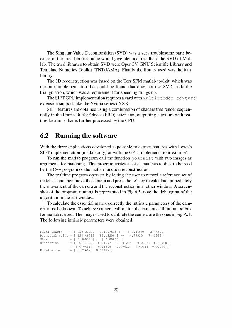
6.1 The images used for matching : first image (a), second image (b),a perpespective view of the whole setup (c), a side view (d) . . . . 22

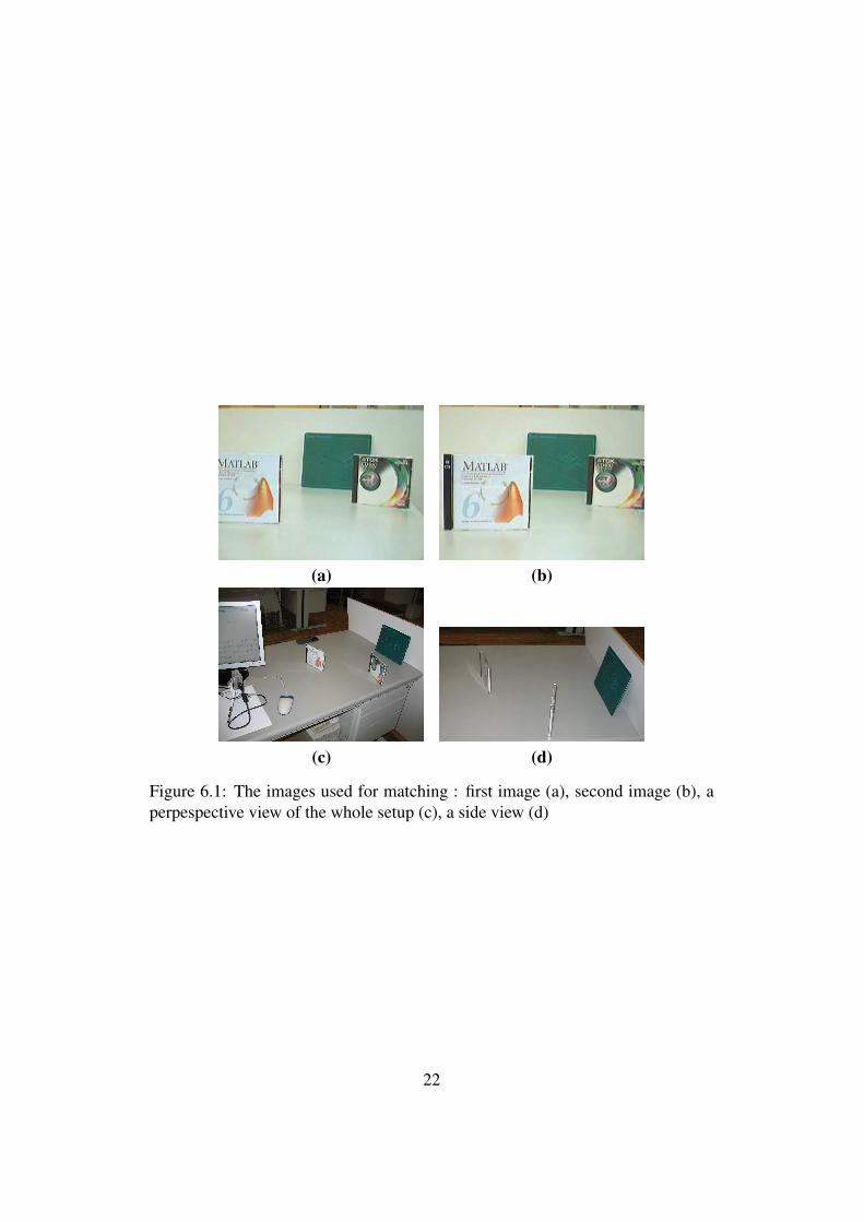
6.2 Reconstruction of the three plane scene: Front view (a), side view(b), top view (c) . . . . . . . . . . . . . . . . . . . . . . . . . . . 23

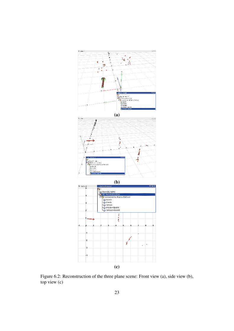
6.3 Screenshot of the debugging of the realtime motion estimation.On the northeast corner we can see the feature matching, on thesoutheast corner is the estimated camera egomotion, and on theleft is the debugging messages. . . . . . . . . . . . . . . . . . . . 24

A.1 Images used for camera calibration. . . . . . . . . . . . . . . . . 27

2

Chapter 1

Introduction

The goal of this project is to develop software for:

1. Feature extraction and matching on the GPU (Graphics Processing Unit).

2. Camera egomotion estimation.

3. 3D reconstruction using triangulation.

The system is composed of three main modules. The first module deals withthe task of feature (high distinguishable image patches) detection, description (setof characteristics used for comparison) and matching (finding the correspondencefrom a different view).

The second module that is for camera motion, takes for input the featurematches and will output the camera matrix P and also the geometric transfor-mation (rotation and translation) between the two views.

The third module uses as input both the matched features and the camera mo-tion to obtain an estimate of the position of the matched points in the world. Thecamera egomotion and the scene reconstruction are achieved less of a scale factor,e.g. the scale is not specified.

The matching was performed based on SIFT features. Due to their computa-tional complexity the SIFT features were casted as a stream processing task thatcan be mapped and performed on a GPU. The use of the GPU makes the task offeature extraction possible in realtime, compared to CPU implementations that dono run in realtime, even in 320× 200 resolutions.

The developed software along with the documentation is made available todownload in the "Modules for Intelligent Autonomous Robot Navigation" (MI-ARN) site [3].

The rest of this report is organized as follows. The related work is describedin chapter 2. A brief introduction to General-Purpose computation on Graphics

3

Processing Units is presented in 3. The detection and tracking of SIFT features isdescribed in chapter 4. The process of estimation of the egomotion is describedin chapter 5. A discussion of the work happens in chapter 6. The conclusion is inchapter 7.

4

Chapter 2

Related Work

In this chapter is described some of recent research concerning feature extraction,description and matching in 2d images and also on camera egomotion estimationbased on these features.

2.1 Features DetectorsScale Invariant Feature Transforms (SIFT) [16] are invariant to rotation, transla-tion and scale variation between images. They are partially invariant to affine dis-tortion, illumination variance and noise because they capture a substantial amountof information about the spatial intensity patterns. They are based on the Dif-ference of Gaussians (DoG) filter that is an approximation of the Laplacian ofGaussian (LoG) focusing on speed. SIFT features have been applied to objectrecognition [17], topological localisation [8], SLAM [7], etc. SIFT features per-formace have been shown the most robust feature detector in [18].

However a significant drawback with the SIFT features is the significant amountof data generated and the computational cost involved. To reduce the compu-tational cost some approaches sacrifice the rotation invariance capability. Theyclaim that avoiding the rotation invariance brings increased discriminative power,as observed in [15, 13]. This is affordable for applications like mobile robot navi-gation, where the camera often only rotates around the vertical axis.

Recently, in [24] SIFT was implemented on a Field Programmable Gate Ar-ray (FPGA) with a good performance. However, the high dimensionality of thedescriptor is a drawback of SIFT at the matching step. For on-line applicationson a regular PC, each one of the three steps (detection, description, matching)should be faster still. In [9] was proposed an algorithm similar to SIFT but insteadof using the DOG detector they used a technique called fast radial blob detec-tor (FRBD) and implemented it on GPU, obtaining results three times faster than

5

SIFT.A feature tracker that runs in realtime even in CPUs is FAST [22], to achieve

this timings it uses points and lines from previous images and does a neighbour-hood search to find the correspondent features.

Ke and Sukthankar [14] applied PCA on the gradient image. This PCA-SIFTyields a 36-dimensional descriptor which is fast for matching, but proved to beless distinctive than SIFT in a second comparative study by Mikolajczyk et al. [19]and slower feature computation reduces the effect of fast matching. In the samepaper [19], the authors have proposed a variant of SIFT, called GLOH, whichproved to be even more distinctive with the same number of dimensions, but it iscomputationally more expensive.

For tracking Lowe proposed a best-bin-first alternative [16] in order to speedup the matching step, but results in lower accuracy. Implementations of SIFTnormally use KD-trees for matching.

2.2 Camera Egomotion estimationThe method described in this work works on planar as well as nonplanar features.There are methods for egomotion estimation based on optical flow that are notsuitable for realtime computation and methods that are based on a search for aplanar patch or a known object. These latest methods are normally used in aug-mented reality applications and imply the existence of a known object in the scene,therefore are not suitable for robot navigation in unknown places.

In [6] are compared several methods of egomotion estimation for robustnessand speed.

In [20] is used the five point relative pose estimation algorithm, using Gröbnerbasis methods for refinement of the camera pose.

A popular approach based on simultaneos localization and mapping (SLAM)is [10] that is available online in form of a library. In that work is presenteda single-camera mapping and localization in real-time at a high frame rate, butrestricted to a desk-like environment. In an extension in [11], the benefits of usinga single wide-angle camera over a normal camera are shown. [21] does an identicalwork but using particle filters instead of kalman filters.

In [23] is used a single camera to generate landmarks as 3D structure of speciallocations in a home environment. Nister [5] tracks a single or stereo camera in realtime at a high frame rate to obtain visual odometry, without explicitly creating amap.

In recent works it was shown that real time estimation of depth from stereocamera configurations is possible, for a good bibliography on this research see[25] that also compute results on the GPU.

6

Chapter 3

Introduction to General-Purposecomputation on Graphics ProcessingUnits

In this work the extraction of SIFT features is computed in the GPU, in the formof shaders i.e. operations on pixels. This chapter gives a brief introduction to thistechnology.

3.1 ApplicationsA recent trend on scientific computing is the General-Purpose computation onGraphics Processing Units. GPGPU are a set of techniques that make use of thecomputational power of current graphics cards with 3d acceleration to computealgorithms that can be casted as texture operations. Examples of applications thathave benefited with the use of GPGPU are: genome sequencing, database oper-ations, computational fluid dynamics, computer vision, computational geometry,neural networks, speech recognition, physics simulations, etc.

GPGPU applications can further benefit from parallel processing if the graph-ics card suports SLI, making the algorithms even faster.

For applications to make use of the GPU without getting into the details of it’soperations some APIs were developed, like sh [4] and brook [1]. For more detailson GPGPU it is adviced a visit to [2].

3.2 GPGPU MethodologyGetting an algorithm in the GPU involves the following steps:

7

1. Setting up the viewport for a 1:1 pixel-to-texel(texture element) mapping.

2. Creating and binding textures containing the input data, associating datawith these textures.

3. Binding a fragment program (acts on texture) that serves as the "computa-tional kernel".

4. Rendering some geometry (usually a screen-sized quad to make sure the"kernel" gets executed once per texel).

After this the result data is rendered to a texture where it can be read back to theCPU using the OpenGL glReadPixels() or glGetTexImage() function. Anotheradvantage is that this texture is ready to be render to a plane for visualization,which is practical in the domain of computer vision.

3.3 Nvidia Cg language for programming shadersCg provides broad shader portability across a range of graphics hardware func-tionality (supporting programmable GPUs spanning the DirectX 8 and DirectX 9feature sets). Shaders written in Cg can be used with OpenGL or Direct3D; Cgis API neutral and does not tie shaders to a particular 3D API or platform. Anexample of a Cg program that exchanges the red with the blue color components,is shown next:

void FragmentProgram(in float2 fptexCoord : TEXCOORD0 ,out float4 colorO : COLOR0,in float4 wpos : WPOS,const uniform samplerRECT FPE1 :TEXUNIT0)

{colorO = texRECT(FPE1, fptexCoord).bgra;

}

8

Chapter 4

Feature detection and tracking

Scale Invariant Feature Transform (SIFT) features were proposed in [16] as amethod of extracting and describing features which are robustly invariant to trans-lation, scaling, rotation, contrast, illumination and small distortions. The SIFTfeature algorithm is based upon finding locations within the scale space of an im-age which can be reliably extracted. The algorithm has four stages.

1. Scale-space extrema detection: The first stage searches over scale spaceusing a Difference of Gaussian(DOG) function to identify potential interestpoints.

2. Keypoint localisation: The location and scale of each candidate point isdetermined and keypoints are selected based on measures of stability.

3. Orientation assignment: One or more orientations are assigned to each key-point based on local image gradients.

4. Keypoint descriptor: A descriptor is generated for each keypoint from localimage gradients information at the scale found in stage 2. An importantaspect of the algorithm is that it generates a large number of keypoints overa broad range of scales and locations.

The first stage finds scale-space extrema located in D(x, y, σ), the DOG func-tion. This phase aims to make features recognizable at many levels of detail. Theeffect of the increment of distance of a scene is identical to a reduction in dimen-tions of the acquired image. This results in a lower level of detail in the image andthat is reforced by the gaussian blur. DOG is computed from the difference of twonearby scaled images separated by a multiplicative factor k:

D(x, y, σ) = (G(x, y, kσ)−G(x, y, σ))∗I(x, y) = L(x, y, kσ)−L(x, y, σ) (4.1)

9

Where L(x, y, σ) is the scale space of an image, built by convolving the imageI(x, y) with the Gaussian kernel G(x, y, σ). Points in the DOG function whichare local extrema in their own scale and one scale above and below are extractedas features. Generation of extrema in this stage is dependent on the frequencyof sampling in the scale space k and the initial smoothing σ0. The features arethen filtered for more stable matches, and more accurately localised to scale andsubpixel image location.

Before a descriptor for the feature is constructed, the feature is assigned anorientation to make the descriptor invariant to rotation. This feature orientationis calculated from an orientation histogram of local gradients from the closestsmoothed image L(x, y, σ). For each image sample L(x, y) at this scale, the gra-dient magnitude m(x, y) and orientation θ(x, y) is computed using pixel differ-ences:

m(x, y) = ((L(x + 1, y)− L(x− 1, y))2 + (L(x, y + 1)− L(x, y − 1))2)12 (4.2)

θ(x, y) = tan−1L(x, y + 1)− L(x, y − 1)

L(x + 1, y)− L(x− 1, y)(4.3)

The orientation histogram has 36 bins covering the 360 degree range of orien-tations. Each point is added to the histogram weighted by the gradient magnitude,m(x, y), and by a circular gaussian with σ variance that is 1.5 times the scale ofthe feature. Additional features are generated for feature locations with multi-ple dominant peaks whose magnitude is within 80 of each other. The dominantpeaks in the histogram are interpolated with their neighbours for a more accurateorientation assignment.

A feature descriptor is created using the gradient magnitude, m(x, y) and ori-entation, θ(x, y) around the feature. These are weighted by a circular gaussianwindow indicated by the overlaid circle. Each orientation histogram is calculatedfrom a 4× 4 pixel support window and divided over 8 orientation bins.

The local gradient data from the closest smoothed image L(x, y, σ) is also usedto create the feature descriptor. This gradient information is first rotated to align itwith the assigned orientation of the feature and then weighted by a gaussian withσ variance that is 1.5 times the scale of the feature. The weighted data is used tocreate a nominated number of histograms over a set window around the feature.Typical feature descriptors [16] use 16 orientation histograms aligned in a 4 × 4grid. Each histogram has 8 orientation bins each created over a support windowof 4×4 pixels. The resulting feature vectors are 128 elements with a total supportwindow of 16 × 16 scaled pixels as can be seen in Fig.4.1 . For a more detaileddiscussion of the feature generation and factors involved see [16].

For matching purposes the Euclidean distance between the keypoints is com-pared. A keypoint is considered “matched” using the nearest neighbor algorithm.

10

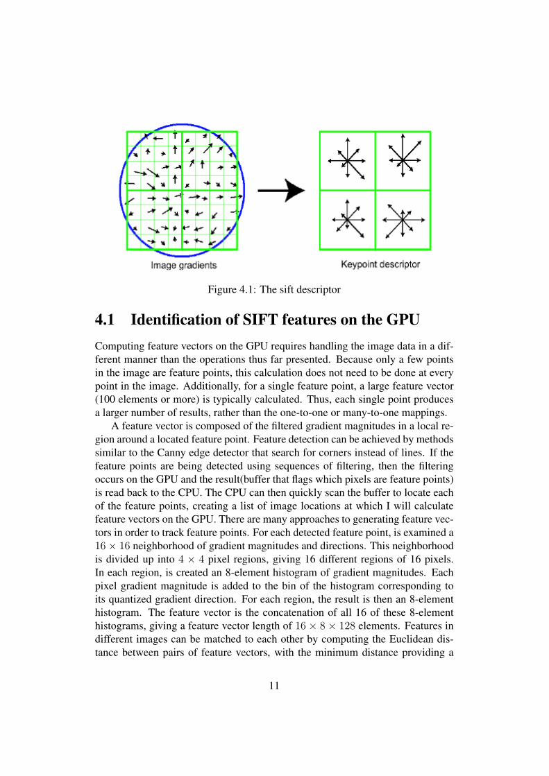
Figure 4.1: The sift descriptor

4.1 Identification of SIFT features on the GPUComputing feature vectors on the GPU requires handling the image data in a dif-ferent manner than the operations thus far presented. Because only a few pointsin the image are feature points, this calculation does not need to be done at everypoint in the image. Additionally, for a single feature point, a large feature vector(100 elements or more) is typically calculated. Thus, each single point producesa larger number of results, rather than the one-to-one or many-to-one mappings.

A feature vector is composed of the filtered gradient magnitudes in a local re-gion around a located feature point. Feature detection can be achieved by methodssimilar to the Canny edge detector that search for corners instead of lines. If thefeature points are being detected using sequences of filtering, then the filteringoccurs on the GPU and the result(buffer that flags which pixels are feature points)is read back to the CPU. The CPU can then quickly scan the buffer to locate eachof the feature points, creating a list of image locations at which I will calculatefeature vectors on the GPU. There are many approaches to generating feature vec-tors in order to track feature points. For each detected feature point, is examined a16× 16 neighborhood of gradient magnitudes and directions. This neighborhoodis divided up into 4 × 4 pixel regions, giving 16 different regions of 16 pixels.In each region, is created an 8-element histogram of gradient magnitudes. Eachpixel gradient magnitude is added to the bin of the histogram corresponding toits quantized gradient direction. For each region, the result is then an 8-elementhistogram. The feature vector is the concatenation of all 16 of these 8-elementhistograms, giving a feature vector length of 16 × 8 × 128 elements. Features indifferent images can be matched to each other by computing the Euclidean dis-tance between pairs of feature vectors, with the minimum distance providing a

11

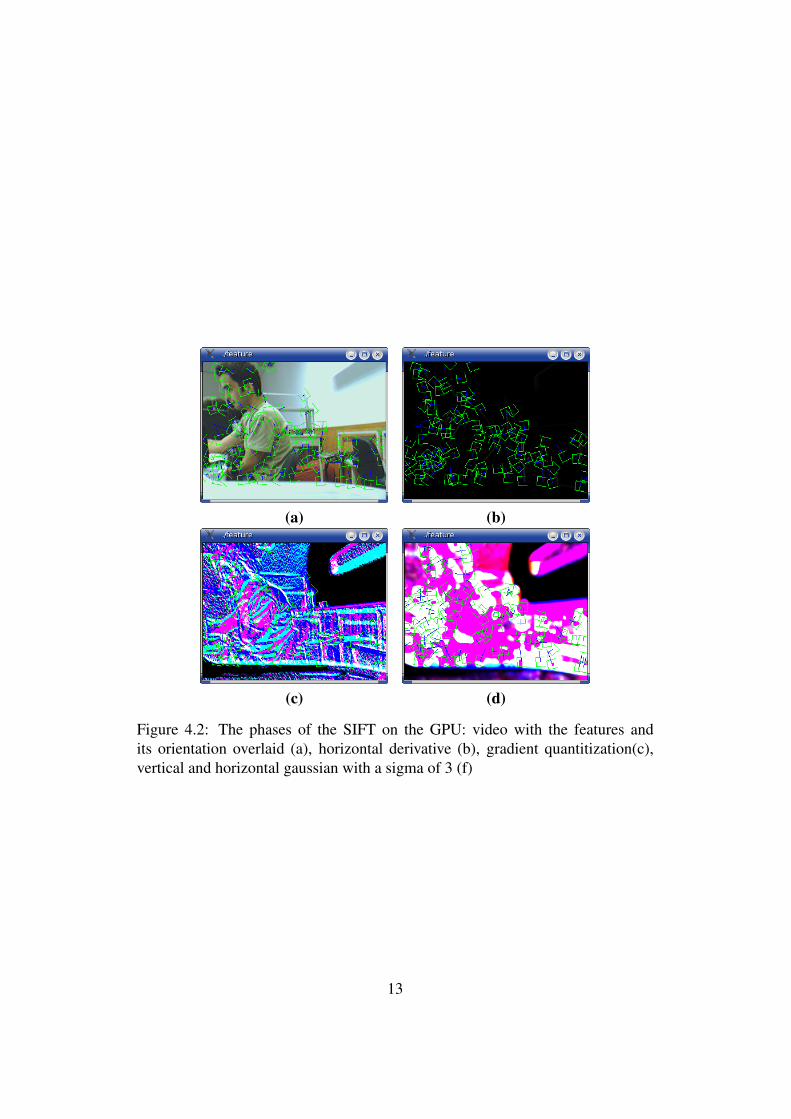
best match. To produce the 128-element feature vector result, are draw rows ofvertices, with one row for each feature, such that each drawn point in the row cor-responds to an element of the feature vector for that feature. Associating texturevalues pointwise allows for the most flexibility in mapping texture coordinates foruse in computing the feature vector. Each point has different texture coordinatesmapped to it to allow a single fragment program to access the appropriate gradi-ents of the local region used to calculate the histogram. In Fig. 4.2 can be seensome of the stages of the SIFT procedure.

12

(a) (b)

(c) (d)

Figure 4.2: The phases of the SIFT on the GPU: video with the features andits orientation overlaid (a), horizontal derivative (b), gradient quantitization(c),vertical and horizontal gaussian with a sigma of 3 (f)

13

Chapter 5

Camera egomotion estimation

The epipolar geometry is the intrinsic projective geometry between two views.It is independent of scene structure, and only depends on the cameras internalparameters and relative pose.

The two perspective views may be acquired simultaneously, for example in astereo rig, or sequentially, for example by a moving camera. From the geometricviewpoint, the two situations are equivalent, but the scene might change betweensuccessive snapshots. Most 3-D scene points must be visible in both views si-multaneously. This is not true in case of occlusions, i.e., points visible only in onecamera. Any unoccluded 3-D scene point M = (x, y, z, 1)T is projected to the leftand right view as ml = (ul, vl, 1)T and mr = (ur, vr, 1)T , respectively. Imagepoints ml and mr are called corresponding points (or conjugate points) as theyrepresent projections of the same 3-D scene point M . The knowledge of imagecorrespondences enables scene reconstruction from images.

Algebraically, each perspective view has an associated 3×4 camera projectionmatrix P which represents the mapping between the 3-D world and a 2-D image.I will refer to the camera projection matrix of the left view as Pl and of the rightview as Pr. The 3-D point M is then imaged as equation 5.1 in the left view, andequation 5.2 in the right view:

ξlml = PlM (5.1)ξrmr = PrM (5.2)

Geometrically, the position of the image point ml in the left image plane Il canbe found by drawing the optical ray through the left camera projection centre Cl

and the scene point M . The ray intersects the left image plane Il at ml. Similarly,the optical ray connecting Cr and M intersects the right image plane Ir at mr. Therelationship between image points ml and mr is given by the epipolar geometry.

14

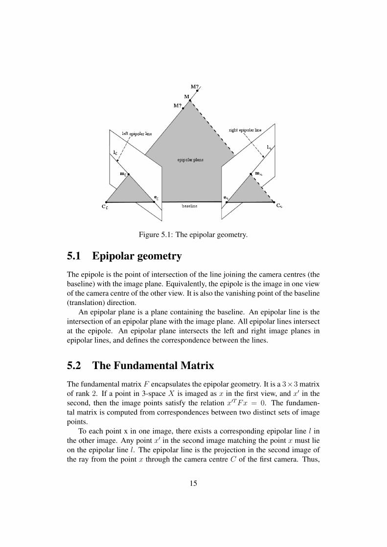
Figure 5.1: The epipolar geometry.

5.1 Epipolar geometryThe epipole is the point of intersection of the line joining the camera centres (thebaseline) with the image plane. Equivalently, the epipole is the image in one viewof the camera centre of the other view. It is also the vanishing point of the baseline(translation) direction.

An epipolar plane is a plane containing the baseline. An epipolar line is theintersection of an epipolar plane with the image plane. All epipolar lines intersectat the epipole. An epipolar plane intersects the left and right image planes inepipolar lines, and defines the correspondence between the lines.

5.2 The Fundamental MatrixThe fundamental matrix F encapsulates the epipolar geometry. It is a 3×3 matrixof rank 2. If a point in 3-space X is imaged as x in the first view, and x′ in thesecond, then the image points satisfy the relation x′T Fx = 0. The fundamen-tal matrix is computed from correspondences between two distinct sets of imagepoints.

To each point x in one image, there exists a corresponding epipolar line l inthe other image. Any point x′ in the second image matching the point x must lieon the epipolar line l. The epipolar line is the projection in the second image ofthe ray from the point x through the camera centre C of the first camera. Thus,

15

there is a map x → l from a point in one image to its corresponding epipolar linein the other image.

Epipolar lines: For any point x in the first image, the corresponding epipolarline is l′ = Fx. Similarly, l = F T x′ represents the epipolar line corresponding tox′ in the second image.

The epipole: for any point x (other than e) the epipolar line l′ = Fx containsthe epipole e′. Thus e′ satisfies e′T (Fx) = (e′T F )x = 0 for all x. It follows thate′T F = 0, i.e. e′ is the left null-vector of F . Similarly Fe = 0, i.e. e is the rightnull-vector of F .

5.3 The Essential MatrixThe essential matrix is the specialization of the fundamental matrix to the caseof normalized image coordinates. The fundamental matrix may be thought of asthe generalization of the essential matrix in which the assumption of calibratedcameras is removed. The essential matrix has fewer degrees of freedom, andadditional properties, compared to the fundamental matrix.

The fundamental matrix is obtained from the Fundamental Matrix with thefollowing relation

E = K ′T FK (5.3)

Where E is the Essential Matrix, F is the Fundamental Matrix and K is the Cal-ibration Matrix. A constrain of E is that it must have two singular values equaland the third equal to zero. This constrain is imposed in this work.

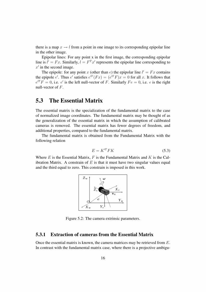
Figure 5.2: The camera extrinsic parameters.

5.3.1 Extraction of cameras from the Essential MatrixOnce the essential matrix is known, the camera matrices may be retrieved from E.In contrast with the fundamental matrix case, where there is a projective ambigu-

16

ity, the camera matrices may be retrieved from the essential matrix up to scale anda four-fold ambiguity. That is there are four possible solutions, except for overallscale, which cannot be determined.

We may assume that the first camera matrix is P = [I|0]. In order to computethe second camera matrix, P ′ , it is necessary to factor E into the product SR ofa skew- symmetric matrix and a rotation matrix.

According to [12] there are four possible solutions for the second camera ma-trix P ′ that are:

P ′ = [UWV T |+ u3] ∨ (5.4)P ′ = [UWV T | − u3] ∨ (5.5)

P ′ = [UW T V T |+ u3] ∨ (5.6)P ′ = [UW T V T | − u3] (5.7)

Figure 5.3: The four possible solutions for calibrated reconstruction from E. Be-tween the left and right sides there is a baseline reversal. Between the top andbottom rows camera B rotates 180◦ about the baseline. Only in (a) is the recon-structed point in front of both cameras.

The geometric result is shown in Fig. 5.3. To test which one is the correct, atest to verify which hypothesis has more points in front of the camera is needed.

17

5.4 Sparse 3D ReconstructionWhat can be reconstructed depends on what is known about the scene and thestereo system. We can identify three cases.

1. If both the intrinsic and extrinsic camera parameters are known, we cansolve the reconstruction problem unambiguously by triangulation.

2. If only the intrinsic parameters are known, we can estimate the extrinsicparameters and solve the reconstruction problem up to an unknown scalefactor. In other words, R can be estimated completely, and t up to a scalefactor.

3. If neither intrinsic nor extrinsic parameters are known, i.e., the only infor-mation available are pixel correspondences, we can still solve the recon-struction problem but only up to an unknown, global projective transforma-tion of the world.

Given sufficient correspondence points from two camera positions it is possi-ble to find both camera matrices P and P ′ and the 3d location of the correspon-dence points Xi. This is possible if the Fundamental matrix can be computeduniquely, so that the scene can be reconstructed up to a projective ambiguity.

The rotation R and translation t obtained previously are used to instantiate acamera pair, and this camera pair is subsequently used to reconstruct the structureof the scene by triangulation.

The rigid displacement ambiguity arises from the arbitrary choice of the worldreference frame, whereas the scale ambiguity derives from the fact that t can bescaled arbitrarily and one would get the same essential matrix (E is defined upto a scale factor). Therefore translation can be recovered from E only up to anunknown scale factor which is inherited by the reconstruction.

For details on the algorithms see [12].

18

Chapter 6

Discussion

6.1 Developed softwareThe implementation is done in three programs, varying the source of matches andif they run online or offline.

1. a matlab prototype that uses the sift program from Lowe to get the matches.

2. a program in c++ and opengl that implements all the matlab operations ex-cept the sift to visualize the 3d reconstruction and camera egomotion.

3. a program that works in realtime to match features from a reference sceneusing a GPU implementation of SIFT and also does the 3d reconstructionand camera egomotion.

Note that the need for the second program was also because that at the mo-ment of writing this code I did not had access to a Nvidia 6XXX card that hasthe features needed to run the SIFT GPU algorithm, so a “transition” programwas needed. The last software was executed on a borrowed laptop from a friend(thanks Carlos), so the code is a little clumsy.

6.1.1 Technical details of the implementation.In the matlab version the estimation of the fundamental matrix was done witheither with the 8 point algorithm or with a ransac version of it. In the C++ versionthe OpenCV library was used for speed and the variety of methods available.

Most of the library for matrix algebra was implemented on the TNT/JAMAlibraries and required alot of functions to be created to make the code transitionfrom matlab possible.

19

The Singular Value Decomposition (SVD) was a very troublesome part; be-cause of the tried libraries none would give identical results to the SVD of Mat-lab. The tried libraries to obtain SVD were OpenCV, GNU Scientific Library andTemplate Numerics Toolkit (TNT/JAMA). Finally the library used was the it++library.

The 3D reconstruction was based on the Torr SFM matlab toolkit, which wasthe only implementation that could be found that does not use SVD to do thetriangulation, which was a requirement for speeding things up.

The SIFT GPU implementation requires a card with multirender textureextension support, like the Nvidia series 6XXX.

SIFT features are obtained using a combination of shaders that render sequen-tially in the Frame Buffer Object (FBO) extension, outputting a texture with fea-ture locations that is further processed by the CPU.

6.2 Running the softwareWith the three applications developed is possible to extract features with Lowe’sSIFT implementation (matlab only) or with the GPU implementation(realtime).

To run the matlab program call the function joaosift with two images asarguments for matching. This program writes a set of matches to disk to be readby the C++ program or the matlab function reconstruction.

The realtime program operates by letting the user to record a reference set ofmatches, and then move the camera and press the ’c’ key to calculate immediatelythe movement of the camera and the reconstruction in another window. A screen-shot of the program running is represented in Fig.6.3, note the debugging of thealgorithm in the left window.

To calculate the essential matrix correctly the intrinsic parameters of the cam-era must be known. To achieve camera calibration the camera calibration toolboxfor matlab is used. The images used to calibrate the camera are the ones in Fig.A.1.The following intrinsic parameters were obtained:

Focal Length = [ 350.38337 351.97616 ] +- [ 3.44094 3.44429 ]Principal point = [ 128.46796 83.18200 ] +- [ 4.79520 7.81536 ]Skew = [ 0.00000 ] +- [ 0.00000 ]Distortion = [ -0.11039 0.21977 -0.01295 0.00841 0.00000 ]

+- [ 0.04837 0.25505 0.00612 0.00411 0.00000 ]Pixel error = [ 0.22669 0.14497 ]

20

6.3 The experience setupTo test the egomotion and reconstruction an experimental setup consisting of acamera on a desk pointing to three planes represented by two cds and a mousepad. The planes have different orientations and stand in the foreground of a whitefeatureless background. The setup was deployed as is shown in Fig. 6.1.

A slight translation of the camera to the left with small clockwise rotation inthe Y axis was executed. And the result can be seen in Fig.6.2.

21

(a) (b)

(c) (d)

Figure 6.1: The images used for matching : first image (a), second image (b), aperpespective view of the whole setup (c), a side view (d)

22

(a)

(b)

(c)

Figure 6.2: Reconstruction of the three plane scene: Front view (a), side view (b),top view (c)

23

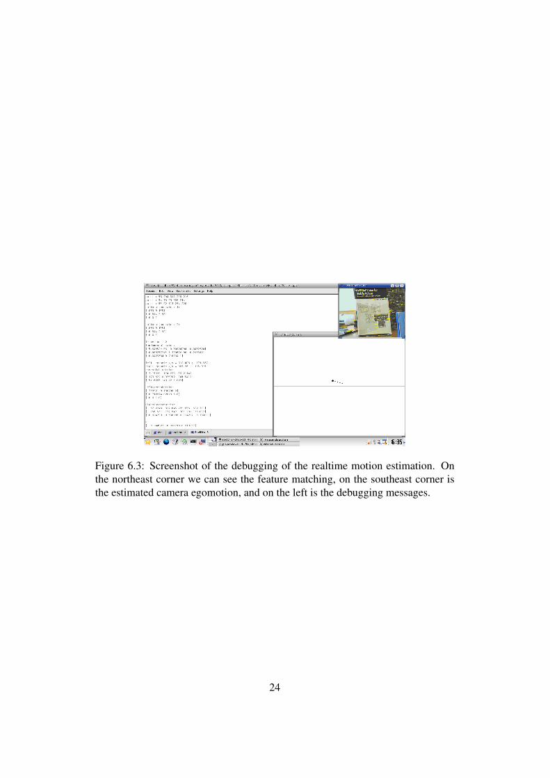
Figure 6.3: Screenshot of the debugging of the realtime motion estimation. Onthe northeast corner we can see the feature matching, on the southeast corner isthe estimated camera egomotion, and on the left is the debugging messages.

24

Chapter 7

Conclusion

A realtime egomotion and sparse reconstrucion algorithm was implemented usingthe GPU for computational speed. The GPU implementation does indeed run inrealtime and with robust matching. The estimation of the Fundamental Matrix bythe OpenCV library is very susceptible to noise which can make the rest of thealgorithm behave strangely sometimes.

All of the steps from a mere camera calibration to 3d reconstruction were stud-ied, along with a research on the state of the art in feature matching and structurefrom motion.

25

Appendix A

Appendix

A.1 Camera Calibration

26

Figure A.1: Images used for camera calibration.

27

Bibliography

[1] The brook gpu programming language,http://graphics.stanford.edu/projects/brookgpu/.

[2] Gpgpu basic math tutorial, http://www.mathematik.uni-dortmund.de/ goed-deke/gpgpu/tutorial.html.

[3] Modules for intelligent autonomous robot navigation, http://miarn.sf.net.

[4] The sh gpu programming language, http://libsh.org.

[5] Visual odometry, IEEE Computer Society, 2004.

[6] X. Armangué, H. Araújo, and J. Salvi, A review on egomotion by meansof differential epipolar geomety applied to the movement of a mobile robot,Pattern Recognition 21 (2003), no. 12, 2927–2944.

[7] T.D. Barfoot, Online visual motion estimation using fastslam with sift fea-tures, Intelligent Robots and Systems, 2005.

[8] M. Bennewitz, C. Stachniss, W. Burgard, and S. Behnke, Metric localizationwith scale-invariant visual features using a single perspective camera, Pro-ceedings of the European Robotics Symposium (EUROS) (Palermo, Italy),2006.

[9] Charles Bibby and Ian Reid, Fast feature detection with a graphics process-ing unit implementation, IMV06 workshop, 2006.

[10] A.J. Davison, Real-time simultaneous localisation and mapping with a sin-gle camera, Proc. International Conference on Computer Vision, Nice, Oc-tober 2003.

[11] A.J. Davison, Y. González Cid, and N. Kita, Real-time 3D SLAM with wide-angle vision, Proc. IFAC Symposium on Intelligent Autonomous Vehicles,Lisbon, July 2004.

28

[12] R. I. Hartley and A. Zisserman, Multiple view geometry in computer vision,second ed., Cambridge University Press, ISBN: 0521540518, 2004.

[13] Luc Van Gool Herbert Bay, Tinne Tuytelaars, Surf: Speeded up robust fea-tures, Proceedings of the ninth European Conference on Computer Vision,2006.

[14] Y. Ke and R. Sukthankar, Pca-sift: A more distinctive representation forlocal image descriptors, 2004.

[15] S Williams L Ledwich, Reduced sift features for image retrieval and in-door localisation, Proceedings of the Australasian Conf. on Robotics andAutomation, 2004.

[16] David Lowe, Distinctive image features from scale-invariant keypoints, Int.J. Comput. Vision 60 (2004), no. 2, 91–110.

[17] David G. Lowe, Object recognition from local scale-invariant features, Proc.of the International Conference on Computer Vision ICCV, Corfu, 1999,pp. 1150–1157.

[18] K. Mikolajczyk and C. Schmid, A performance evaluation of local descrip-tors, 2003.

[19] Krystian Mikolajczyk and Cordelia Schmid, A performance evaluation oflocal descriptors, IEEE Transactions on Pattern Analysis and Machine In-telligence 27 (2005), no. 10, 1615–1630.

[20] David Nistér, An efficient solution to the five-point relative pose problem,IEEE Trans. Pattern Anal. Mach. Intell. 26 (2004), no. 6, 756–777.

[21] Mark Pupilli and Andrew Calway, Real-time camera tracking using a par-ticle filter, Proceedings of the British Machine Vision Conference, BMVAPress, September 2005, pp. 519–528.

[22] Edward Rosten and Tom Drummond, Fusing points and lines for high per-formance tracking., IEEE International Conference on Computer Vision,vol. 2, October 2005, pp. 1508–1511.

[23] S. Se, D. Lowe, and J. Little, Mobile robot localization and mapping withuncertainty using scale-invariant visual landmarks, 2002.

[24] Piotr Jasiobedzki Stephen Se, Ho-Kong Ng and Tai-Jing Moyung, Visionbased modeling and localizationfor planetary exploration rovers, Interna-tional Astronautical Congress, 2004.

29

[25] L. Wang, L. Miao, M. Gong, R. Yang, and D. Nistér, High quality real-timestereo using adaptive cost aggregation and dynamic programming, Interna-tional Symposium on 3D Data Processing, 2006.

30