wavemimo methodology: numerical wave generation of a

J. Appl. Comput. Mech., 7(4) (2021) 2129–2148 DOI: 10.22055/jacm.2021.37617.3051

ISSN: 2383-4536 jacm.scu.ac.ir

Published online: August 21 2021

Shahid Chamran

University of Ahvaz

Journal of

Applied and Computational Mechanics

Research Paper

WaveMIMO Methodology: Numerical Wave Generation of a

Realistic Sea State

Bianca Neves Machado1 , Phelype Haron Oleinik2 , Eduardo de Paula Kirinus3 , Elizaldo Domingues dos Santos4 , Luiz Alberto Oliveira Rocha5 , Mateus das Neves Gomes6 ,

José Manuel Paixão Conde7 , Liércio André Isoldi8

1 Federal University of Rio Grande do Sul (UFRGS), Interdisciplinary Department, 030 Highway, km 92, Tramandaí, 95590-000, Brazil, Email: [email protected]

2 Federal University of Rio Grande (FURG), School of Engineering, km 8 Itália Avenue, Rio Grande, 96201-900, Brazil, Email: [email protected]

3 Federal University of Paraná (IFPR), Center for Marine Studies, Beira-Mar Avenue, Pontal do Paraná, 83255-976, Brazil, Email: [email protected]

4 Federal University of Rio Grande (FURG), School of Engineering, km 8 Itália Avenue, Rio Grande, 96201-900, Brazil, Email: [email protected] 5

University of Vale do Rio dos Sinos (UNISINOS), Polytechnic School, 950 Unisinos Avenue, São Leopoldo, 93022-750, Brazil, Email: [email protected]

6 Federal Institute of Paraná (IFPR), Campus Paranaguá, 453 Antonio Carlos Rodrigues Street, Paranaguá, 83215-750, Brazil, Email: [email protected]

7 NOVA University of Lisbon (UNL), NOVA School of Science and Technology, Lisbon, 1099-085, Portugal, Email: [email protected]

8 Federal University of Rio Grande (FURG), School of Engineering, km 8 Itália Avenue, Rio Grande, 96201-900, Brazil, Email: [email protected]

Received June 02 2021; Revised August 09 2021; Accepted for publication August 17 2021.

Corresponding author: Liércio André Isoldi ([email protected])

© 2021 Published by Shahid Chamran University of Ahvaz

Abstract. This paper presents a methodology that allows the numerical simulation of realistic sea waves, called WaveMIMO methodology, which is based on the imposition of transient discrete data as prescribed velocity on a finite volume computational model developed in Fluent software. These transient data are obtained by using the spectral wave model TOMAWAC, where the wave spectrum is converted into a series of free surface elevations treated and processed as wave propagation velocities in the horizontal (x) and vertical (z) directions. The processed discrete transient data of wave propagation velocity are imposed as boundary conditions of a wave channel in Fluent, allowing the numerical simulation of irregular waves with realistic characteristics. From a case study that reproduces the sea state occurring on March 31st, 2014, in Ingleses Beach, in the city of Florianópolis, state of Santa Catarina, Brazil, it was concluded that the WaveMIMO methodology can properly reproduce realistic conditions of a sea state. In sequence, the proposed methodology was employed to numerically simulate the incidence of irregular realistic waves over an oscillating water column (OWC) wave energy converter (WEC). From these results, the WaveMIMO methodology has proved to be a promising technique to numerically analyze the fluid-dynamic behavior of WECs subjected to irregular waves of realistic sea state on any coastal region where the device can be installed.

Keywords: Ocean waves, irregular waves, computational modeling, Fluent, TOMAWAC.

1. Introduction

The urgent need for clean and renewable energy sources is well known. Among the possibilities, there is an important and still poorly explored resource: the ocean. The harnessing of ocean wave energy can significantly contribute to addressing the growing global demand for electric energy [1].

According to Mørk et al. [2], the total theoretical potential of wave energy is 32,000 TWh/yr, having the same order of magnitude as the energy consumption on the planet, which was 22,385.81 TWh in 2015 [3]. However, it is estimated that the value that can be used, due to geographical, technical, or economic constraints, is one order of magnitude lower [4]. The most energetic waves on the planet are generated between latitudes of 30° and 60° by extratropical storms. Wave energy availability varies seasonally, with variation typically higher in the northern hemisphere [5].

Ocean wave energy is energy that has been transferred from the wind to the ocean. The waves store this energy as potential energy (in the water mass displaced in relation to the mean sea level) and kinetic energy (in the motion of the water particles) [6]. In addition, the waves are very efficient in the transfer of energy and can travel long distances on the surface of the ocean with little loss of energy. However, in coastal regions, the energy density decreases due to the interaction with the sea floor [7, 8].

To date, several devices have been studied, developed and, in many cases, tested in real scale for the conversion of wave energy into electricity, but none of them has been consolidated from the commercial point of view. As the characteristics of the installation site are very singular, they must be considered to choose the appropriate wave energy converter (WEC) [9, 10].

In this sense, it is a fundamental point to understand how the WEC behaves when subjected to the incidence of the sea waves.

Bianca Neves Machado et. al., Vol. 7, No. 4, 2021

Journal of Applied and Computational Mechanics, Vol. 7, No. 4, (2021), 2129–2148

2130

For this reason, computational fluid dynamics (CFD) modeling has been widely used to relate equipment functionalities and environmental variables.

However, countless studies found in the literature address a numerical generation of regular waves [11–15], as well as its incidence over the WEC, e.g., overtopping devices [16–21], oscillating water column (OWC) devices [15, 22–27] and submerged horizontal plate (SHP) devices [28–32]. This simplification is valid since it provides important information about the working principle of WECs, but the obtained results for its available power do not properly reflect reality.

Another approach that can be found in the literature relies on the study of irregular waves, especially applying the JONSWAP and Pierson-Moskowitz [33] wave spectra. Some works use the incident wave spectrum over the WECs, allowing a more realistic representation of the problem, e.g., OWC [25, 27, 34–36], overtopping devices [37] and floating body converters [38–41]. Other studies approach only the numerical generation of irregular waves [42–48]. However, this approach requires for the spectral shape to match a defined function, which is rarely the case in real sea states.

In the literature, one can also find the case when a wave train is measured in situ using wave buoys [49] or produced using physical models [50]. This is the ideal case when actual wave measurements are used to force a numerical simulation so that the waves imposed are the best possible representation of the real scenario. However, this type of data is restricted to a single point in space and a limited period of time, so it can only be used in a determined set of studies. Furthermore, the cost of the equipment necessary for acquiring this type of data is prohibitive for installation for the sole purpose of a numerical study.

Given the above and specifically regarding the computational modeling approach of irregular waves, it should be noted that, so far, as stated by Romanowski et al. [51], there are no well-defined methodologies for CFD numerical simulation of irregular sea states. Hence, CFD is still not widely used to investigate the effect of realistic ocean waves over vessels and marine structures. Nevertheless, in the literature, there are numerical methodologies for irregular wave propagation, as follows.

In Jacobsen et al. [52], the library waves2Foam of OpenFOAM software was extended to a generic free surface water wave generation and its absorption. It includes the solver, based on the interFoam solver, the volume of fluid (VOF) solver in OpenFOAM, and some utilities for pre- and postprocessing. The absorption method applies a relaxation zone technique (active sponge layers) and the relaxation zones can take arbitrary shapes. To show the method’s ability to model wave propagation and wave breaking, benchmark tests were carried out. A large range of regular wave theories is supported, as well as irregular waves.

Higuera et al. [53, 54] developed a numerical methodology for realistic wave generation associate with active wave absorption in OpenFOAM software, aiming for applications in coastal engineering studies. This methodology is implemented in a solver known as IHFoam. Higuera et al. [53] presented the theoretical background for the proposed boundary conditions for simultaneous wave generation and its active absorption; the validation of this methodology is presented in Higuera et al. [54]. The active absorption method is based on the linear shallow water theory, which means that it works very well in shallow water but is unable to absorb deep-water waves.

Dos Reis et al. [42] presented a methodology for forecasting and early warning of wave overtopping in ports/coastal areas. The system downloads sea-wave characteristics predicted offshore, up to 180 h, every day. These data correspond to results obtained through WAVE-WATCH III. To transfer to the port entrance and then into the port, SWAN and DREAMS are applied, which are a spectral wave model and a mild slope wave model, respectively. The DREAMS model provides wave characteristics in front of each structure, which are then used as inputs to the neural network tool NN_OVERTOPPING2, together with cross-sectional characteristics of the maritime structures. NN_OVERTOPPING2 gives an estimate of mean overtopping discharges per unit length of the structure crest.

Shen et al. [55] and Shen and Wan [56] developed an irregular wave generation model capable of maintaining the wave amplitudes by automatic adjustments of the input wave spectrum based on measured of free surface elevation in a numerical channel. These authors used a white noise spectrum to generate the incoming irregular waves to evaluate the ship motion responses. The procedure replaces a decade of simulations in regular waves with one single run to obtain a complete curve of linear motion response, considerably reducing computation time. The computations were made using a solver based on OpenFOAM and used a damping zone (sponge layer) to dissipate waves at the end of the channel. Its validation was carried out with several cases with different wave spectra.

The software ANSYS Fluent [57] also has available different types of wave theories, regular and irregular, to be used with the VOF method. To avoid wave reflection, there is a numerical beach considering in the momentum equation a damping sink term. Lisboa et al. [58] presented a detailed methodology for regular and irregular wave propagation in a channel using ANSYS Fluent. The irregular waves were based on a JONSWAP spectrum, which obtained satisfactory results.

Dealing specifically with WEC investigations, Ransley et al. [50] presented a numerical study of the fluid-dynamic behavior analysis of WEC systems submitted to extreme waves, which was validated with experimental data. A nonlinear CFD methodology was developed in OpenFOAM using waves2Foam [52] and the six degrees of freedom (6DOF) body motion solver, including the propagation of design waves, the free surface behavior around structures, the pressure on the structure’s surface, the motion of floating structures, and the loading in mooring lines.

Gatin et al. [59] and Choi et al. [60] presented the coupling of the pseudo-spectral high-order spectral (HOS) method and a nonlinear viscous two-phase CFD model for irregular wave simulations in Open-FOAM software. The CFD model is based on solution decomposition via the spectral wave explicit Navier-Stokes equation (SWENSE) method, allowing efficient coupling with arbitrary potential flow solutions. In both references, validations were presented, showing the applicability of the methodology for extreme wave modeling.

Miquel et al. [61] evaluated the performance of several wave generation techniques and wave absorption methods used in CFD numerical wave tanks. To do so, the REEF3D open-source code was employed, which is based on the Reynolds-averaged Navier-Stokes (RANS) equations, allowing two-phase flow simulations. The wave generation and absorption were promoted by the relaxation method, Dirichlettype method, and active wave absorption. Among the simulated cases, irregular waves were successfully tested.

Mendonça et al. [47] applied the methodology from dos Reis et al. [42] to characterize the sea-wave at the Azores archipelago in terms of the corresponding wave power for a period of 10 years at various points around each island in winter and summer.

Romanowski et al. [51] proposed a methodology for CFD irregular ocean wave simulations, aiming to model complex and realistic marine environments. From the statistical analysis of irregular sea proposed by a wave spectrum, its decomposition into key factors allows defining meshing and time step methodologies for CFD modeling. The presented examples were carried out with the JONSWAP spectrum and Star CCM+ software. These authors used and presented a MATLAB code to generate a time history of a JONSWAP spectrum defined by the key variables, significant wave height and peak period and using a randomness factor. In their simulations, these authors solved the RANS equations using the standard - turbulence model and the VOF method.

Therefore, aiming to provide a cost-effective alternative to in situ wave measurements, and at the same time allowing the representation of a realistic sea state in a numerical study of sea waves, the present work proposes a methodology for the numerical generation of irregular waves, which reproduces the sea state of a coastal region of interest. With this approach, it will

WaveMIMO Methodology: Numerical Wave Generation of a Realistic Sea State


2131

be possible to numerically evaluate the fluid-dynamic behavior of WECs when submitted to a realistic sea state related to the intended installation spot. The contribution of this work is the coupling between the software TOMAWAC (TELEMAC-Based Operational Model Addressing Wave Action Computation) and Fluent, enabled by the innovative way to impose the boundary conditions of prescribed velocity for wave generation in Fluent.

TOMAWAC [62, 63] is a spectral model for coastal hydrodynamic simulations able to reproduce a realistic sea state; however, it fails to study the fluid-dynamic behavior of WECs. In opposition, Fluent [57] is a CFD software able to numerically simulate the operating principle of WECs; but it would present difficulties in modeling the coastal propagation of waves as TOMAWAC does.

Therefore, the main goal of this work is to propose a methodology that applies the TOMAWAC results as boundary conditions at Fluent for the numerical generation of irregular realistic sea waves, aiming to simulate WECs submitted to its incidence. To do so, the sea state of the Ingleses Beach (located in the city of Florianópolis, state of Santa Catarina, Brazil) that occurred on March 31st, 2014, was reproduced by the proposed methodology. After that, the incidence of these realistic irregular waves was considered over an OWC device, showing the applicability of the WaveMIMO methodology.

2. TOMAWAC

The computational model used for the hindcast simulation was TOMAWAC, part of the Open TELEMAC–Mascaret modeling system 1 . TOMAWAC is a third-generation sea-state solving wave model based on the equation of wave action density conservation [62]. In a general situation of propagating waves in a nonhomogeneous and nonstationary environment, e.g., an environment under the action of currents and/or sea level variation, the wave action is preserved, being taken into account the energy exchange processes that the waves are subject to when propagating. The physical processes considered by TOMAWAC include wind-driven generation and propagation; bottom-friction-induced dissipation; wave breaking; bathymetry and current-induced refraction; shoaling; whitecapping dissipation; and nonlinear triad and quadruplet interactions. However, TOMAWAC does not consider phase dependent processes such as diffraction and reflection, so its usage is not recommended where these processes prevail [63]. TOMAWAC splits the directional spectrum of wave action (�) into a finite number of wave frequencies (��) and directions (��) (called a discrete directional spectrum) and solves the wave action density equation for each component (��, ��).

2.1 Superficial and Boundary Conditions for TOMAWAC

To perform the numerical simulations, data from NOAA’s (National Oceanic and Atmospheric Administration) wave forecasting model WAVEWATCH III2 [64] and from the NCEP/NCAR Reanalysis [65] were used to represent the liquid and superficial boundaries of the model, respectively.

The model started from rest, and the surface boundary was set to winds from the NCEP/NCAR Reanalysis 1, with a temporal resolution of 6 h and a spatial resolution of 1.875° (T62 Gaussian Grid). These data were bilinearly interpolated to the unstructured mesh used to simulate the sea state. The oceanic boundaries were set by the imposition of the integrated parameters: spectral significant wave height (Hs), spectral peak period (Tp), and spectral peak mean direction (Dp). The data obtained from WAVEWATCH III have a spatial resolution of 0.5° (approximately 56 km in the study region) and the temporal resolution of 3 h. The bathymetry data used to represent the sea bottom were obtained from the GEBCO3 (General Bathymetric Chart of the Oceans) in deeper regions, and on the continental shelf and near the coastline, the bathymetric data were obtained from the DHN (Diretoria de Hidrografia e Navegação4 of the Brazilian Navy).

3. Fluent

Fluent is CFD software, based on the finite volume method (FVM), able to numerically simulate water wave propagation in both deep and shallow water. To do so, Fluent solves the Reynolds averaged Navier-Stokes (RANS) equations, using the volume of fluid (VOF) technique to identify the free surface. Proposed by Hirt and Nichols [66], the VOF method is a multiphase model used to solve flows composed of two or more immiscible fluids through the concept of a volumetric fraction (�). Therefore, in the present study, Fluent was employed for the numerical generation of a realistic sea state in a wave channel, as well as for the incidence of these irregular waves over WECs, solving the continuity equation, the Navier-Stokes equation for a water-air mixture, and the volumetric fraction transport equation [67-68], respectively, given by:

( ) 0vt

ρρ

∂+∇⋅ =

∂

� (1)

( ) ( ) ( )v vv p g Stρ ρ µτ ρ

∂+∇⋅ =−∇ +∇⋅ + +

∂

�� (2)

( ) 0vt

αα

∂+∇⋅ =

∂

� (3)

where � is the fluid density, t is the time, v�

is the velocity vector, p is the static pressure, � is the viscosity, τ is the stress

deformation tensor, gρ�

is the buoyancy force, g�

is the gravity acceleration vector, and S�

are the external body forces.

Once the mass and momentum conservation equations are solved for the mixture between air and water, average values for

the density and viscosity are calculated as follows [68]:

water water air airρ α ρ α ρ= + (4)

water water air airµ α µ α µ= + (5)

1 www.opentelemac.org 2 http://polar.neep.noaa.gov/waves/wavewatch 3 www.gebco.net 4 www.mar.mil.br/dhn/chm/box-cartas-nauticas/cartas.html



2132

In addition, the computational model developed in the Fluent software uses the first-order upwind scheme for the treatment of advective terms, the PRESTO (pressure staggering option) method for spatial discretization of the pressure, and the PISO (pressure-implicit with splitting of operators) method for pressure-velocity coupling [67]. Moreover, the geo-reconstruction scheme is applied for the volumetric fraction discretization [69].

The generation of regular waves in Fluent is performed by the imposition of components of horizontal (�) and vertical () velocity of the wave as prescribed boundary conditions. These velocity components are obtained using regular wave theories (Airy, 2nd-order Stokes, etc.). This methodology is widely used for WECs evaluation when submitted to regular waves in a variety of studies, as in Machado et al. [14], Martins et al. [18], Han et al. [19], Horko [22], Gomes et al. [24], Gaspar et al. [26], Seibt et al. [28], Chen et al. [70], and Yamaç and Koca [71].

It is still possible to avoid the effect of wave reflection at the end of the wave channel in the model by employing a technique called numerical beach. In other words, the numerical beach technique dissipates the energy of the waves that reach the end of the wave channel. To do so, a damping sink term is added in the momentum equation, given by [72–74]:

2

1 2

11

2fs s

e sb fs

z z x xS C V C V V

z z x xρ ρ

− − =− + − − − (6)

where �1 is the linear damping coefficient, �2 is the quadratic damping coefficient, V is the velocity along the z direction, � is the density, � is the vertical position, �� and �� are the vertical positions of the free surface and bottom, � is the horizontal position, and � and �� are horizontal positions of the beginning and end of the numerical beach. As recommended by Lisboa et al. [58], the coefficients of linear and quadratic damping can be set equal to 20 and zero, respectively.

4. WaveMIMO Methodology

The WaveMIMO5 methodology allows the numerical simulation of irregular waves in a wave channel, representing the waves of a realistic sea state for a particular coastal region. To do so, a wave spectrum is obtained from the spectral wave model TOMAWAC and then, it is transformed into a time series of free surface elevations. This time series is appropriately treated using the procedure explained in sections 4.2 to 4.4 and transformed into the orbital velocity components of the water particles. Finally, the transient discrete data from the propagation velocity of the realistic waves are imposed as velocity inlet boundary conditions of the wave channel in Fluent, thereby allowing irregular waves to be numerically simulated with realistic characteristics. Figure 1 shows a summary of the WaveMIMO methodology. It is worth mentioning that the irregular waves only can be generated in Fluent software due the innovative way of subdivided the inlet region of the wave channel, allowing that discrete values of the vertical and horizontal velocity components of the wave along the water column are imposed as boundary conditions in each subdivision. General guidelines on the WaveMIMO methodology starting from TOMAWAC and ending in Fluent are presented in appendix. Highlighting that the WaveMIMO methodology can also be used to generate regular waves.

Fig. 1. Summary flowchart of the WaveMIMO methodology. Rectangles represent a step of the methodology, and arrows represent the action to go from one step to another. The text to the right describes each item.

5 The first letter of the surname of B. N. Machado, L. A. Isoldi, W. C. Marques and P. H. Oleinik originated the name of this methodology for

irregular wave imposition on the wave channel.



2133

Fig. 2. Overview of the study area: (a) The location of the mesh in South America; (b) The island of Florianópolis; (c) Ingleses Beach and the location of the wave channel.

4.1 Study Area

The chosen location to insert the hypothetical wave channel is the Ingleses beach in the island of Florianópolis, state of Santa Catarina, Brazil; based on the work of Oleinik et al. [75], who evaluated the annual behavior of the waves on the South-Southeastern Brazilian Shelf. Figure 2 shows an overview of the study area. The numerical domain used for TOMAWAC comprises the Brazilian coast from the city of Mostardas (state of Rio Grande do Sul), at its southernmost point, to Santos (state of São Paulo), at its northern end, totaling approximately 1000 km of coastline. The mesh also extends approximately 700 km towards the sea, as presented in Fig. 2a. The shape of the coastline was taken from the GSHHG6 (global self-consistent, hierarchical, high-resolution geography) database [76]. The numerical mesh is an unstructured triangular mesh with variable spatial resolution. At the oceanic boundary, the edges of the triangular elements have approximately 0.1° (≈ 11 km), progressively reducing to 0.03° (≈ 3 km) at the continental shelf slope, and 0.005° (≈ 500 m) near the coastline. At the study area, the elements are progressively refined to approximately 30 m from one mesh node to another. It should be noted that this location was adopted due to the possibility to validate the obtained numerical results from TOMAWAC with data monitored in situ by the wave buoy operated by the Brazilian PNBOIA (Programa Nacional de Boias), from the previous work of Oleinik et al. [75].

The island of Florianópolis is located approximately in the center of the coastline of the domain (Fig. 2b), and Ingleses Beach is located at the northern part of the island (Fig. 2c). Ingleses Beach has a NW–SE orientation, and the wave channel is practically perpendicular to the coastline, as shown by the line in Fig. 2c. The oceanic end of the wave channel is located at the coordinates 27°25’59.1”S and 48°23’19.6”W, and the other end touches the coastline at 27°26’6.14”S and 48°23’28.5”W.

The simulated period with TOMAWAC was from January 1st to March 31st, 2014, to allow for the model to stabilize; the data used to generate the velocity profiles for the wave channel simulation in Fluent were obtained from the last hour of March 31st. The data used to impose the velocity profile on the wave channel were taken from the node farthest away (point “P” in Fig. 2c, 327 m from the coastline) from the coast on the representative wave channel (indicated by the red lines in Fig. 2c).

TOMAWAC’s results were taken at the oceanic end of the wave channel (point “P” in Fig. 2c) to force the fluid-dynamic simulations on Fluent. The used data were the wave spectrum (the directional spectrum integrated along with the directions) and the wave’s integrated parameters, i.e., spectral significant wave height (Hs) and spectral peak period (Tp). The directional spectrum was integrated along the discretized directions to simplify the imposition of the boundary conditions in the 2D wave channel simulation in Fluent. This simplification does not impact the results because the chosen location is near the coastline, so due to refraction, the waves travel in a single direction perpendicular to the coastline.

Finally, the wave spectrum was then transformed into an equivalent time series of sea surface elevations using the method described in the following sections. From this, the discrete orbital velocity components of waves in horizontal (u) and vertical (w) directions are defined and imposed as boundary conditions of prescribed velocities at the subdivided inlet region of the wave channel in Fluent, generating the irregular waves corresponding to the realistic sea state of TOMAWAC.

4.2 Converting Wave Spectra into Sea Surface Elevation

Large-scale sea state modeling is only possible because wave models use wave spectra to represent the sea surface behavior at a given point and time. The sea surface under the action of waves has an elevated rate of change in small distances and periods of time, and their representation requires a sampling rate of, at least half of their period, otherwise, the sampling rate is less than the Nyquist frequency, and the data will be aliased [77]. This high sampling rate makes the time-domain representation of sea surface data impractical for large-scale applications.

However, the sea surface behavior under wind-wave action is considered a stochastic process [77], which allows the representation of its general behavior with a semi-stationary function with a very lower rate of change in time and space. This function, namely, the wave spectrum, is the frequency-domain representation of the sea state.

6 www.ngdc.noaa.gov/mgg/shorelines/gshhs.html



2134

Usually, sea surface elevation data are measured by wave buoys, and these data are condensed into a spectrum using a Fourier transform. The Fourier transform of a real-valued function (such as the sea surface elevation) results in a complex-valued function, whose real and imaginary parts are merged to compose the spectrum. This operation yields the variance spectrum of the sea surface, and the phase data are discarded following the assumption that the phase of wind-waves is randomly distributed in the interval [0; 2�] [77].

However, for small-scale processes, such as the fluid-dynamic modeling of wave channel and WEC devices, the time domain representation is more useful because it allows representing short-scale processes that prevail in these situations.

As stated above, the wave spectrum contains only information on the amplitude of the waves, using the assumption of the wave phase randomly distributed in the interval [0; 2�]. If one tries to simply apply an inverse Fourier transform to the wave spectrum, the lack of phase data (which is then taken to be null) behaves as a resonance effect of every wave component, resulting in a wave that resembles a sawtooth wave.

To properly transform the spectrum back into an equivalent series of sea surface elevation (�) data, one must provide the missing random phase data to the IFFT (inverse fast Fourier transform) algorithm. With these data, one can write the Fourier

transform of the sea surface elevation, ( ),ηF as the combination of the amplitude data from the spectrum and the generated

random phase data. The additional phase spectrum is crucial in this process because without it, the IFFT would assume the phase to be zero for all components, and thus, a resonance of the wave components would appear in the time series of surface elevation.

Then, the sea surface elevation caused by the action of the waves can be obtained by applying the inverse Fourier transform

(usually by means of an IFFT implementation) to the aforementioned ( ),ηF obtaining �.

The generated random sea surface elevation series, if long enough to eliminate statistical bias from the random numbers, will have the same characteristics as the original spectrum. The spectral variance and the variance of the sea surface elevation are the same; the spectral significant wave height and the significant wave height measured from the time series (using, for example, the zero-up crossing method) are the same; and, more importantly, the spectrum of said time series is identical to the original.

It is worth noting that depending on the combination of the variance spectrum and the random phase spectrum, the resonance effect mentioned earlier might happen at smaller scales, producing a taller wave due to superposition of the linear components. This effect is reduced by increasing the sample size as described above.

4.3 Obtaining the Velocity Field from the Sea Surface Elevation

According to Holthuijsen [77], one of the basic assumptions of the wave spectra is that the sea state is composed by the sum of a finite number of plane monochromatic waves that can, individually, be described by the linear wave theory of Airy [78]. With this theory, the free surface elevation and the horizontal and vertical components of the velocity field caused by the passage of the waves are, respectively [6]:

( )cosA kx tη ω= − (7)

( )

( )( )

coshcos

sinh

k h zu A kx t

khω ω

+ = − (8a)

and

( )

( )( )

sinhsin

sinh

k h zw A kx t

khω ω

+ = − (8b)

Equations (8a) and (8b) describe the velocity profile along the water column (� coordinate) of a monochromatic wave with amplitude � = H/2, length � = 2�/�, and period � = 2�/� propagating in a medium with average depth ℎ; being � the wave number and � the wave frequency.

As a consequence of the method used to transform the spectrum, the mean sea level is taken to be zero ( 0),η = so the wave

amplitude can be assumed to be equal to �. Therefore, to calculate the velocity field, it is still necessary to determine the wavelength and period.

Since the generated time series for � cannot be described by an analytical function and the clear distinction of what is a wave does not hold anymore because of the random character added to the data, one can resort to the usual wave counting methods. For this paper, the zero-up crossing method is used to count the waves and measure them [6]. Figure 3 exemplifies the process used to calculate the wave period and length for the time series of sea surface elevation.

First, the waves are separated from each other (Fig. 3a) using the zero-up crossing method, which consists of counting as a “wave” the segment of the time series between every other instant when the value of � is zero. After the waves are split, the period is obtained by simply calculating the time interval between the first up-cross and the next, which is, effectively, the duration of the wave (Fig. 3b). One major problem with this method is the discontinuities caused by the discretely counting the waves. To counteract this issue, the discrete periods were smoothed using a cosine interpolation technique (Fig. 3b).

With the wave period calculated, the wavelength can be obtained by solving for � the dispersion relation, given by [77]:

( )2 tanhgk khω = (9)

where the angular wave frequency � is related to wave period T by � = 2�/T, the angular wave number � is related to wavelength � by � = 2�/�, and � is the acceleration of gravity.

To avoid the iterative solution of Eq. (9), the explicit approximation proposed by Beji [79] was adopted:

( )

0 0

0

1

tanh

mµ µµ

µ

+ = (10)

where m = 1.09e-(1.55+1.3�0+0.216 �

0²), � = �ℎ = 2�ℎ/�, and �0 = �0ℎ = 4�2ℎ/��2. This approximation can be used to directly calculate the wave

number � with a maximum relative error of less than 0.044%, a significant improvement compared to the widely used approximation by Eckart [80], with an accuracy of 5%. Using Eq. (10), the time series of wavelength (Fig. 4) can be calculated using the previously obtained wave period.



2135

Fig. 3. Illustration of the procedure to obtain � from �: (a) Sample time series of �. (b) Discrete measured waves and calculated time series of wave period �.

Fig. 4. Calculated time series of wavelength �.

Fig. 5. Illustration of the computational domain of the wave channel. Geometry used for generation of regular waves: (a) Procedure 1: Imposition of continuous � and using Eqs. (8a) and (8b) - see the solid blue line in the inlet region; (b) Procedure 2: Imposition of discrete � and from data files

generated from Eqs. (8a) and (8b) - see the subdivision of the inlet region.

Now, finally, Eqs. (8a) and (8b) can be employed to calculate the velocity field at arbitrary points along the water column (�) at every time step of the simulation.

In the case where a spectrum of the velocity fields is also available, it is possible to skip this step altogether and use the IFFT process described in the previous section to obtain the velocity fields. However, since TOMAWAC is a 2D model that simulates only the wave spectrum at the surface, the velocity profiles along the water column are not available, so this step is necessary.

4.4 Regular and Irregular Wave Generation in Fluent

As earlier mentioned the Fluent software was already used in several works addressed to the propagation of regular waves, as well as to study the fluid-dynamic behavior of WECs over the incidence of these waves. The conventional way of generating waves in Fluent, named here as Procedure 1, imposes the horizontal and vertical velocities of the regular waves, defined by Eqs. (8a) and (8b), at a continuous inlet region of the wave channel (solid blue line in Fig. 5a).

However, in the present study, it is proposed an alternative way to prescribe the wave velocity components (called as Procedure 2) by means the tool Table Data/Boundary Profiles in Fluent software. For this, a geometric particularity is required: the computational domain region in which the prescribed velocities are imposed in the wave channel needs to be divided into sub-regions (dashed light and dark green line in Fig. 5b). Thereby, the corresponding discrete values for the wave velocity components u and w along the water column should be defined at the center of each subdivision of the wave channel inlet.



2136

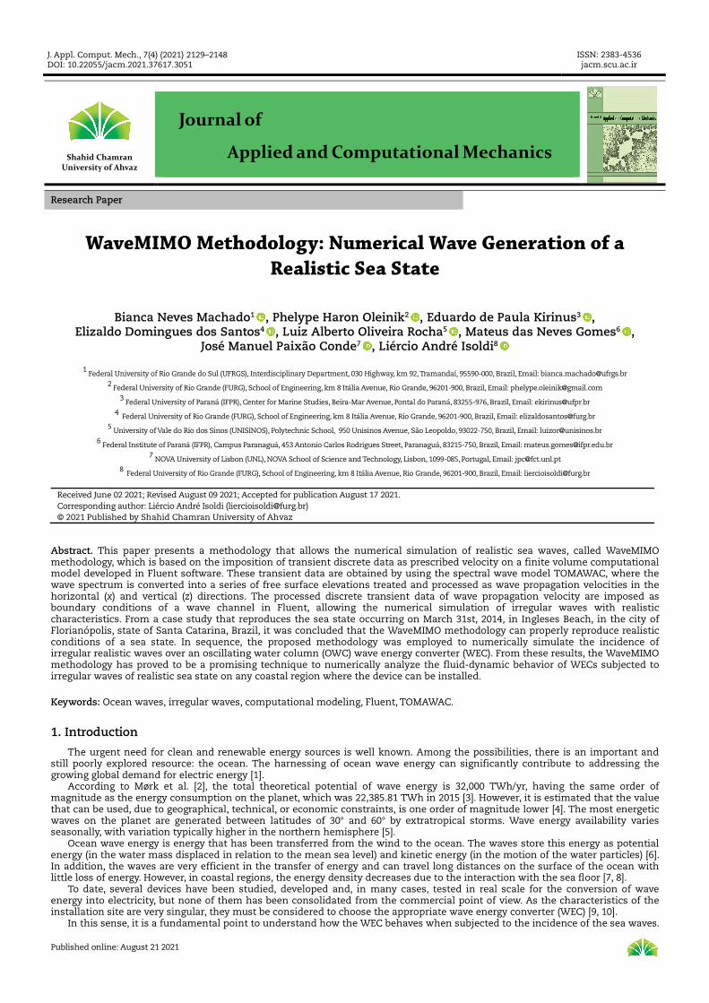
Fig. 6. Validation time series of TOMAWAC (continuous line) for the studied period, comparing with buoy data (dots): (a) Hs and (b) Tp.

Regarding the other boundary conditions, considering Fig. 5, on the upper region of the left boundary and the upper boundary

of the wave channel, the atmospheric pressure is prescribed as a boundary condition (dashed red line). In the right end of the wave channel, a numerical beach is defined, as explained in Section 3, to dampen the incoming waves. On the right boundary of the channel, after the numerical beach, a hydrostatic profile (dashed blue line) is imposed on the fluid in order to avoid reflection. On the bottom channel (solid black line), a nonslip with impermeability boundary condition is imposed, which means that the velocities are prescribed as null. For the initial conditions, the fluid is considered at rest (dashed gray line).

In its turn, for the irregular wave generation, which is the focus of the present work, necessarily the alternative way to prescribe the wave velocities (Procedure 2) should be adopted. Like this, the discrete transient values of the velocity components obtained from TOMAWAC for different depths along the water column are imposed as prescribed velocity boundary conditions in the Fluent software. The other boundary conditions are the same employed for the regular wave generation. Both for the generation of regular waves and for the generation of irregular waves, the numerical analysis consists of finding a solution for the transient and laminar water-air flow. More details about the numerical model can be found in Machado et al. [14], Gomes et al. [36], and dos Santos et al. [81].

5. Results

In this section, initially, a validation of the computational modeling performed in TOMAWAC and a verification of the computational modeling developed in Fluent were carried out. Then, the results of the WaveMIMO methodology, which couples these two numerical models, are presented and discussed.

It is important to inform that the numerical simulation in TOMAWAC was performed in a workstation Intel Core i7-4960X clocked at 3.60 GHz and 32 GB of RAM; while all numerical simulations in Fluent were carried out in a workstation Intel Core i5-7500 clocked at 3.40 GHz and 16 GB of RAM.

5.1 Validation of the Computational Model Developed in TOMAWAC

To validate the parameterization performed in TOMAWAC, its results were compared to data measured by a wave buoy operated by the Brazilian PNBOIA (Programa Nacional de Boias). The buoy is located at the coordinates 31°31’12” S and 49°48’36” W, with an average depth of 200 m off the coast of Santa Catarina state. The buoy data are available for almost the entire simulated period (between January and March 2014), except for the last week of January.

Figure 6 compares the data measured by the buoy (dots) and the corresponding time series from TOMAWAC (continuous line). The available data for comparison are the spectral significant wave height (Hs) and spectral peak period (Tp).

Qualitatively, the results of the model seem to correlate to the observations on the simulated period, with very few occurrences of large discrepancies. The comparison for Tp (Fig. 6b) is apparently slightly off more frequently, which can be attributed to the discrete nature of this variable and the very likely misalignment of TOMAWAC’s and the buoy’s spectra.

To quantify the fitting of both datasets, one can use a few common error metrics [75, 82–86]. The comparison is done for the average of the variables and their standard deviation. The error metrics used are the root mean square error (RMSE) and the scatter index (SI) defined by [83, 85, 86]:

( )2

1

n

i ii

R E

RMSEn

=

−

=∑

(11)

and

i

RMSESI

R= (12)

where R� are the reference values (which here are the data measured by the buoy), E� are the estimated values (which here are the

TOMAWAC’s results), � is the number of points in the dataset, and iR is the average of reference values.

Table 1 shows the error metrics calculated for the studied period. From the average of Hs one can conclude that TOMAWAC slightly underestimates the measured data. This is a common conclusion in this type of comparison [75, 83, 85] because the model usually fails to correctly represent too extreme phenomena. In addition, the variability (given by the standard deviation) is approximately the same, and the RMSE and consequently the SI are acceptable for this type of simulation.

From Table 1, the average and standard deviation of Tp show high similarity between measured and simulated datasets, showing that, on average, the sea behavior is the same. In this kind of analysis, it is usually recommended to proceed with the RMSE due to problems related to zero and, mainly, because the difference R� − E� is squared, so larger differences, which are severe parameterization errors, weight more in the final RMSE value than smaller differences, which are minor processes not considered by the model. The RMSE for both Hs (0.44 m) and Tp (1.52 s) is around the usual values for sea wave models [82–85]. Additionally, the scatter index shows that the overall comparison for Tp is better than for Hs in the studied period. Therefore, the spectral wave model developed in TOMAWAC can be considered adequately validated, as already presented in previous works [75, 83–85].



2137

Table 1. Error metrics calculated using the buoy data and TOMAWAC’s results.

Parameter PNBOIA TOMAWAC

Hs

Average [m] 1.70 1.61 Standard Deviation [m] 0.57 0.46

RMSE [m] 0.44

0.26 SI [-]

Tp

Average [s] 9.15 9.08 Standard Deviation [s] 2.13 1.40

RMSE [s] 1.52 0.17 SI [-]

Table 2. Integrated parameters used for the representative monochromatic linear wave scenario.

Parameter Symbol Value

Spectral significant wave height [m] Hs 0.3545 Spectral peak period [s] Tp 11.12

Wavelength [m] L 96.91

Wave channel depth [m] h 8.5035

Table 3. Time step influence.

Δt (s) Δt/T RMSE [m] MAE [m] Processing time [h]

0.20 0.0179 0.0090 0.0076 0.3167

0.10 0.0089 0.0087 0.0074 0.6833

0.09 0.0081 0.0087 0.0074 0.9000

0.08 0.0072 0.0087 0.0074 0.9333

5.2 Verification of the Computational Model Developed in Fluent

To verify the computational model used for the regular wave generation in Fluent, its results were compared with the free surface elevation given by Eq. (7). The regular waves were generated using the two procedures previously described to impose the prescribed velocity as boundary conditions on the computational domain inlet: Procedure 1- the widely adopted imposition of the analytical Eqs. (8a) and (8b); and Procedure 2 - the proposed alternative way for the imposition of the discrete transient velocity of wave propagation in the horizontal (�) and vertical (�) directions.

For this purpose, the integrated spectrum parameters (Hs and Tp) were used to represent a sea state equivalent to the irregular scenario, but using a monochromatic linear wave calculated from these parameters. The integrated parameters are calculated by TOMAWAC by integrating the spectrum along with the discretized frequencies. Moreover, the mean wavelength was calculated iteratively using the peak period on the dispersion relation (Eq. (9)). The integrated values used are summarized in Table 2.

In other words, the regular waves defined in Table 2 are representative of the irregular wave data obtained from TOMAWAC and were considered in this verification procedure. Its numerical propagation was performed in the wave channels presented in Figs. 5a and 5b, having horizontal and vertical dimensions of 327 m and 12 m (based on Martins et al. [18]), respectively.

Initially, the discretization of the computational domain was performed with a stretched mesh, as proposed by Mavriplis [87], with the refinement in the free surface region, as recommended by [88]. Thus, the domain was vertically discretized into 60 computational cells in the region with only water, 20 cells per wave height in the free surface region and 20 cells in the region with only air; horizontally, the discretization was 50 computational cells per wavelength.

Regarding the analysis of the numerical beach, wave reflection was observed when using the recommendation of 2·L (twice the wavelength of representative regular wave) for the beach length indicated in Lisboa et al. [45] since the generated numerical wave presented considerable differences when compared to the solution given by Eq. (7). Aiming to reduce these differences, the numerical beach length of 2.5·L (two and a half times the wavelength) was also tested. To do so, numerical simulations of 100 s were carried out with a numerical probe positioned at 275 m from the beginning of the wave channel. For this preliminary study, the regular wave generated in the channel with the numerical beach of 2.5·L in length presented smaller differences in comparison with results of Eq. (7). This fact can be proved by the value of the largest crest obtained for the 2·L and 2.5·L numerical beaches, of 0.1441 m and 0.0119 m, respectively. As seen, the numerical beach with a length of 2.5L damped the waves in a more efficient way and was thus adopted in this study.

Thereafter, the time step influence was analyzed through the RMSE (see Eq. (11)) and the mean absolute error (MAE), defined as [85]:

1

ni i

i

R EMAE

n=

−=∑ (13)

adopting as reference the regular wave described by Eq. (7). Table 3 shows the five investigated Δ� values, as well as the corresponding RMSE and MAE for a numerical probe positioned at

50 m from the beginning of the wave channel (Wave Monitor 50 m on Fig. 5). For all cases, a total simulation time of � = 180 s was used.

From Table 3, it is possible to infer that the RMSE and MAE remain constant from Δ� = 0.10 s. Therefore, aiming to reduce the processing time, the time step of Δ� = 0.10 s was adopted.

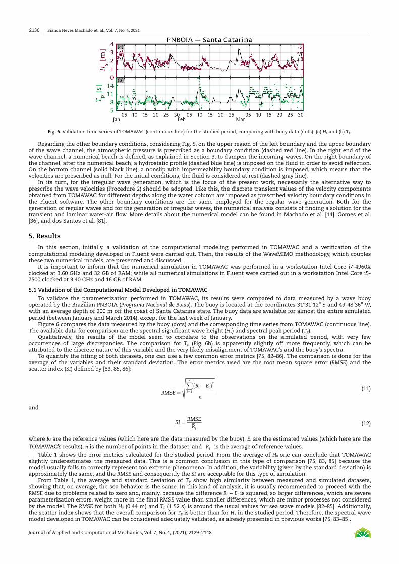
Next, using the same mesh refinement and time step defined by means Procedure 1, Procedure 2 was also applied to generate the same regular waves already simulated, aiming to prove that the proposed alternative way of boundary condition imposition does not significantly changes the outcome of the simulation. Figure 7 shows the free surface elevation numerically generated by using Procedure 1 and Procedure 2, as well as the free surface elevation given by the Airy wave theory (Eq. (7)), at position � = 50 m for the time interval of 13 s ≤ � ≤ 180 s.

From Figure 7, it is possible to qualitatively note that there is no significant difference between the results obtained with Procedure 2 when compared with those obtained with Procedure 1 (adopted as reference). In addition, one can observe that the crests and troughs of the waves are in phase concerning the Airy wave theory (Eq. (7)). The quantitative difference between the numerical solution obtained with Procedure 2 and the solution given by Eq. (7) is RMSE of 4.00% and MAE of 3.42%. In its turn, when comparing the results of Procedure 2 with the results of Procedure 1, values of RMSE = 0.80% and MAE = 0.70% were achieved.



2138

Fig. 7. Verification of regular wave generation in Fluent.

Fig. 8. Illustration of the computational domain of the wave channel used for the generation of irregular waves with the WaveMIMO methodology (same as Fig. 5b) with the bathymetry of Ingleses Beach added.

It is worth highlighting that Procedure 1 has already been verified and validated in other studies, such as in Machado et al. [17],

Martins et al. [18], Han et al. [19], Gomes et al. [24], Gaspar et al. [26], Seibt et al. [28], Chen et al. [70], Yamaç and Koca [71], Goulart et al. [89]. It is also worth mentioning that this verification of Procedure 2 is fundamental for the proposed WaveMIMO methodology since the subdivision of the inlet region of the computational domain is required for the generation of irregular waves, as detailed in the next section.

5.3 WaveMIMO Methodology Verification

To verify the WaveMIMO methodology, numerical simulations with the wave channel shown in Fig. 8 were performed. To do so, its velocity inlet boundary was subdivided into 14 equal segments, and in each segment, the component values of the irregular wave propagation velocity of the realistic sea state in the horizontal (�) and vertical () directions were imposed.

These data were originally obtained from the directional spectrum of TOMAWAC (according to Section 4), transformed into a temporal series of elevation of the free surface and used to calculate the velocity components (as described in Sections 4.2 and 4.3); finally, they were imposed in Fluent as boundary conditions (according to Section 4.4).

5.3.1 Spectral Analysis

Based on the assumption that the sea state can be described by a stationary function, namely, the variance spectrum of the free surface elevation (�), as explained in Section 4.2, it is possible, instead of a time-domain analysis, to perform a frequency domain analysis of the water surface elevation.

Therefore, a time series of surface elevation at the inlet region of Fig. 8 (left end of the wave channel, i.e., at x = 0 m) was collected, in addition to another time series located in the propagation zone in the wave channel (at x = 65 m downstream from the inlet - Wave Monitor 65 m on Fig. 8), as well as the time series of elevation used to generate the velocity profiles.

The analysis at the first point (x = 0 m) is required because it shows that the transformation of the free surface from TOMAWAC into a velocity profile and its imposition in Fluent results in the expected behavior of the free surface, proving that the proposed methodology is consistent. The analysis in the second point (x = 65 m) aims to demonstrate Fluent’s capability to propagate the irregular waves imposed on the inlet region along the wave channel, allowing is application in WECs investigations.

The time series used have 3600 s of duration with an interval of 0.05 s, resulting in 216 data points of �. The three time series were transformed into their spectrum using the fast Fourier transform (FFT) implementation from the FFTW library (fastest Fourier transform in the West) [90]. The spectrum was calculated and then resampled taking the average of each 16 consecutive data points to reduce the intrinsic noise of the FFT, as suggested by Holthuijsen [77].

Regarding the numerical simulation in Fluent, also considering a temporal discretization of 0.05 s, a mesh sensitivity test was performed by adopting five mesh refinements. It was used as reference the representative regular wave of the realistic sea state (see Table 2). Hence, the first spatial discretization (named mesh M1) was adopted considering the recommendations of Mavriplis [87] and Gomes et al. [88], as earlier explained. From M1, successive refinements in the free surface region were proposed, generating meshes with twice (M2), three times (M3), four times (M4), and five times (M5) more refined than the mesh M1, as indicated in Table 4.



2139

Table 4. Spatial refinements of free surface region for irregular wave generation in Fluent.

Mesh Vertical cells dimension [m] Horizontal cells dimension [m] Processing time [h]

M1 0.01773 1.93820 31.20

M2 0.00887 0.96910 50.12

M3 0.00591 0.64607 77.20

M4 0.00443 0.48455 101.40

M5 0.00355 0.38764 153.02

Table 5. Quantitative evaluation of free surface elevation at the inlet of the wave channel.

Mesh RMSE [m] MAE [m]

M1 0.068 0.054

M2 0.054 0.043

M3 0.053 0.042

M4 0.052 0.041

M5 0.051 0.040

Figure 9 presents the resultant spectrum obtained at the inlet region of the wave channel in Fluent for each mesh of Table 4, in

comparison with the spectrum from TOMAWAC. The original spectrum of elevation (TOMAWAC) exists only in the region between 1 s and 30 s because, as previously described, TOMAWAC was discretized with 25 frequencies ranging from 1 s to 30 s. In other words, the TOMAWAC frequency interval is between 0.033 Hz (30 s) and 1 Hz (1 s).

Figure 9 shows the variance spectral density S as a function of the frequency � or the period �. It can be observed that Fluent reproduces the imposed waves with good agreement because the spectrum of the free surface at the wave channel inlet (Fluent – 0 m) is very similar to the original spectrum from TOMAWAC, especially for the meshes M4 and M5. The slight differences observed come from the transformation processes between TOMAWAC and Fluent; and from the spatial discretization of the computational domain in Fluent. Therefore, as expected, the proposed WaveMIMO methodology is verified since the imposition of velocities in Fluent reproduces the same realistic sea state that is represented by the original spectrum of TOMAWAC. It is worth to highlight that there is no significant difference between the results of meshes M4 and M5 in Fig. 9; however an increment around 50% in processing time occurs if M5 is adopted instead M4 (see Table 4).

This aforementioned similarity can also be observed in Fig. 10, where the variation of free surface elevation at the inlet region of the wave channel in Fluent is compared with the one from TOMAWAC. Qualitatively, the same trend can be noticed, i.e., the same irregular wave behavior of TOMAWAC occurs in all cases reproduced in Fluent by means the WaveMIMO methodology. Aiming to quantify the relative differences, Table 5 presents the RMSE and MAE having the free surface elevation of TOMAWAC as reference.

From Table 5, it is evident that the proposed methodology is robust to transform the spectral data obtained in TOMAWAC into velocity components to be imposed as boundary conditions in Fluent, thus allowing the generation of irregular waves. Again it is noticed that there is no significant improvement if compared the results of mesh M5 with those of mesh M4.

These slight differences can be perceived when the variation of free surface for the cases in Fluent and TOMAWAC are plotted together in interval times of 50 s, as depicted in Fig. 11; highlighting that all cases simulated in Fluent preserve the irregular behavior of the realistic sea state predict by TOMAWAC.

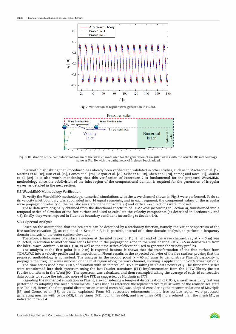
Thereafter, in order to evaluate the propagation of irregular waves, the results monitored by the numerical probe located at 65 m from the wave channel inlet (see Fig. 8) were considered. For each mesh refinement (see Table 4), Fig. 12 shows the spectrum at 65 m in Fluent in comparison with the original spectrum from TOMAWAC.

Regarding the comparison in the propagation zone of the wave channel, in a general way it is possible to infer a good agreement for the medium- and low-frequency waves. However, the high-frequency waves presented a discrepancy that can be reduced by using a more refined spatial discretization in Fluent. This aspect can be observed for the mesh M1 that is able to propagate waves with frequencies below 0.25 Hz (period above 4 s). Furthermore, the meshes M4 and M5 are able to numerically simulate waves with frequencies below approximately 0.33 Hz (period above 3 s).

Fig. 9. Comparison of spectra at the inlet of the wave channel in Fluent and the realistic spectrum of TOMAWAC.



2140

Fig. 10. Free surface elevation at the inlet of the wave channel in Fluent and the realistic free surface elevation of TOMAWAC: (a) TOMAWAC, (b) Fluent - M1, (c) Fluent - M2, (d) Fluent - M3, (e) Fluent - M4, and (f) Fluent - M5.

Here, it is important to present some remarks about it: i) more refined meshes that are suitable to numerically simulate the high-frequency waves will need a large, if not prohibitive, processing time; ii) the main motivation to the development of the WaveMIMO methodology is concerned with the computational modeling applied to the study of WECs; and iii) the amount of energy available in high-frequency waves is not so significant for harnessing by the WECs, as already observed for OWC WECs in Gomes et al. [24] and overtopping WECs in Martins et al. [18]. Therefore, this limitation of the proposed methodology should not significantly impact the fluid-dynamic evaluation of WECs or the determination of its available power.

As in the Fluent numerical simulations the wind action was not considered, in addition to the differences caused during data transformation between TOMAWAC and Fluent and the influence of spatial discretization on Fluent, other possible cause for the energy loss for high-frequency waves can be related with the fact that waves of less than 7 s, classified as “sea waves”, whose defining characteristic, which differentiates them from longer waves (called “swells”), is the need for wind action to maintain their propagation. Sea waves exist in the region of wave generation and dissipate as soon as the wind stops, or they incorporate enough energy to become “swell” waves that can propagate long distances without wind action.

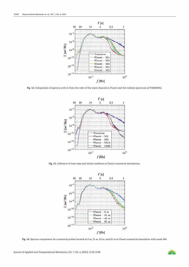
Still concerning the limitation on reproducing the high-frequency waves in Fluent, the influence of two other possible causes was also investigated: temporal discretization and initial condition. Taking into account the improvement obtained with mesh M2 related to mesh M1 (see Fig. 12), the mesh M2 was adopted here as reference. Then, the time step of 0.05 s previously used was reduced to 0.025 s, being the case M2A; while the case M2B adopted a total simulation time of 7200 s, being considered only the final 3600 s thus avoiding the rest initial condition. Figure 13 shows these results together with the TOMAWAC, M1 and M2 spectra.



2141

Fig. 11. Free surface elevation comparison for different interval time.

One can observe in Fig. 13 that the spectrum from M2A case is practically the same obtained with case M2, indicating that the time step of 0.05 s used in simulations is adequate and its reduction cannot improve the results. In its turn, the results of case M2B indicated that the rest initial condition used in simulations is more adequate than having as initial condition an agitated wave channel. Therefore, based on these results as well as in the results of the mesh sensitivity test, it is possible to indicate the spatial discretization in Fluent as the main reason for the non-reproduction of the high-frequency waves.

Finally, to show the influence of distance from the inlet region in the irregular wave propagation, other two numerical probes were considered at 21 m and 43 m in addition to the located at 0 m (Fig. 9) and 65 m (Fig. 12). Figure 13 illustrates the spectrum for each one of these four monitoring points for the mesh M4 (see Table 4).

The results of Fig. 14 showed that there is no significant difference between the spectra at 43 m and 65 m, indicating stabilization related to the already explained WaveMIMO limitation in reproducing high-frequency waves with periods lower than 3 s.

It is worth informing that all numerical simulations performed in this section were simulated using the aforementioned settings for the numerical beach. The elevations measured downstream from the numerical beach were approximately 2.5% of those upstream, ensuring that the numerical dampening of the incoming irregular waves was enough to eliminate disturbances due to wave reflection at the end of the wave channel.



2142

Fig. 12. Comparison of spectra at 65 m from the inlet of the wave channel in Fluent and the realistic spectrum of TOMAWAC.

Fig. 13. Influence of time step and initial condition in Fluent numerical simulations.

Fig. 14. Spectra comparison for numerical probes located at 0 m, 21 m, 43 m, and 65 m in Fluent numerical simulation with mesh M4.



2143

5.4 WaveMIMO methodology application for numerical analysis of WECs

In order to show the main application of the proposed methodology, a case study was numerically simulated considering the incidence of irregular and regular waves related to the realistic sea state of Ingleses Beach (see Fig. 2c) over an OWC WEC. The goal here is to prove that the high-frequency waves of the realistic sea state has no significant effect for the numerical analysis of WECs; as well as that there is significant magnitude difference in the available power of WECs when representative regular waves of the sea state are adopted instead its irregular waves.

5.4.1 WaveMIMO methodology applied to an OWC device

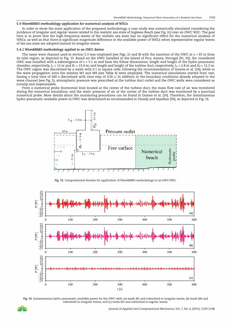
The same wave channel used in section 5.3 was employed (see Figs. 2c and 8) with the insertion of the OWC at x = 65 m from its inlet region, as depicted in Fig. 15. Based on the OWC installed at the Island of Pico, Azores, Portugal [91, 92], the considered OWC was installed with a submergence of s = 5.1 m and have the follow dimensions: length and height of the hydro-pneumatic chamber, respectively, Lc = 12 m and Hc = 13.4 m; and length and height of the turbine duct, respectively, Ld = 2.8 m and Hd = 11.3 m. The OWC region was discretized by a mesh with 0.1 m square cells, following the recommendation of Gomes et al. [24]; while in the wave propagation zone the meshes M1 and M4 (see Table 4) were employed. The numerical simulations started from rest, having a total time of 600 s discretized with time step of 0.05 s. In addition to the boundary conditions already adopted in the wave channel (see Fig. 5), atmospheric pressure was prescribed at the turbine duct outlet and the OWC walls were considered as nonslip and impermeable.

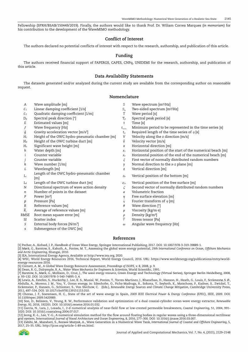
From a numerical probe (horizontal line) located at the center of the turbine duct, the mass flow rate of air was monitored during the numerical simulation; and the static pressure of air at the center of the turbine duct was monitored by a punctual numerical probe. More details about the monitoring procedures can be found in Gomes et al. [24]. Therefore, the instantaneous hydro-pneumatic available power in OWC was determined as recommended in Dizadji and Sajadian [93], as depicted in Fig. 16.

Fig. 15. Computational domain for application of WaveMIMO methodology to an OWC WEC.

Fig. 16. Instantaneous hydro-pneumatic available power for the OWC with: (a) mesh M1 and submitted to irregular waves, (b) mesh M4 and submitted to irregular waves, and (c) mesh M1 and submitted to regular waves.



2144

One can observe in Fig. 16 that qualitatively there is no considerable difference between the results obtained with meshes M1 (Fig. 16a) and M4 (Fig. 16b) for the OWC available power. However, if the regular representative wave of the sea state is considered, one can infer a considerable difference in available power (Fig. 16c). To quantify these differences, the root mean square (RMS) available power was calculated, achieving 3.76 W, 3.82 W, and 1.04 W, respectively, for the cases a, b, and c of Fig. 16. Taking as a reference the result obtained with mesh 4 (Fig. 16a), a relative difference of only 1.57% occurs for the mesh M1 results (Fig. 16b), indicating that de high-frequency waves have no significant effect over the available power of the OWC. Besides, it is worth to emphasize that the processing time required to simulate with mesh M4 (Fig. 16b) is 325% higher than the processing time necessary with mesh M1.

On the other hand, if the RMS available power reached in the representative regular wave simulation (Fig. 16c) is compared with result from mesh M4 (Fig. 16a), a difference of 72.77% occurs, indicating that the WEC analyzes performed with regular waves do not lead to realistic results.

Moreover, another aspect that comes from this case study is the importance of geometric evaluation and optimization of WECs. A significantly improvement in the energy conversion capability should be achieved if the OWC dimensions be defined in agreement to the local sea state.

6. Conclusion

This article presented the WaveMIMO methodology, a procedure that allows the numerical simulation of a realistic sea state, by the imposition of discrete transient velocity data as boundary conditions for the generation of irregular waves. To do so, a wave spectrum from TOMAWAC was transformed into a time series of surface elevation, which was then used to calculate time series of wave propagation velocity in the horizontal (�) and vertical () directions. Finally, these transient velocity components were imposed as boundary conditions in Fluent, generating the irregular realistic sea state waves. It is worth emphasizing that the main application of the proposed methodology is addressed to the numerical study of WECs, making it possible to assess the fluid-dynamic behavior of these devices when submitted to realistic irregular waves.

Therefore, to prove the capability of the WaveMIMO methodology, several analyses were performed, indicating the following: The wave spectrum on the surface at the inlet boundary of the wave channel in Fluent is very similar to the original

TOMAWAC spectrum; The free surface elevation at the inlet of the wave channel in Fluent has a good agreement with the free surface of TOMAWAC,

presenting RMSE of 0.05 m and MAE of 0.04 m; The wave spectrum propagated in the wave channel is well reproduced for low- and medium-frequency waves (i.e. for waves

with periods higher than 4 s) if compared with the original spectrum; The wave spectrum propagated in the wave channel presented differences when compared with the original spectrum for

the high-frequency waves with periods lower than 4 s (with coarser mesh M1) or 3 s (with more refined meshes M4 and M5); The possible causes for the energy loss related to the high-frequency waves were investigated, being the spatial

discretization of the computational domain in Fluent the one with greater influence; As low- and medium-frequency waves are the most relevant for wave energy conversion, the limitation in reproducing high-

frequency waves does not significantly impact the numerical simulation of the fluid-dynamic behavior of WECs; Despite the limitation of propagating high-frequency waves, the definition of the available power of WECs submitted to

realistic irregular waves is much more accurate than the obtained with the widely used approach based on the representative regular waves from the sea state; and

For studies concerned with the geometric optimization of WECs in Fluent, the proposed methodology allows to reproduce the same sequence of irregular waves over each geometry, being an advantage if compared with the wave spectrum approach (e.g., JONSWAP or Pierson-Moskowitz).

Therefore, the proposed WaveMIMO methodology is able to reproduce a realistic sea state from TOMAWAC in Fluent, in a range of periods between 3 s and 30 s (or frequencies between 0.03 Hz and 0.33 Hz), allowing numerical simulations of the operating principle of WECs when submitted to these irregular waves. It is worth mentioning that the irregular wave generation in Fluent was only possible due to the subdivision of the inlet region of the wave channel, enabling to impose as boundary conditions discrete values for the horizontal and vertical velocity components of the waves. This way of prescribing the wave velocities in Fluent is a scientific contribution to the wave energy area, justifying the WaveMIMO methodology application. However, its application is not limited to the wave energy investigations; being possible do apply the WaveMIMO methodology for studies involving the incidence of realistic irregular waves over other naval, coastal and oceanic structures (e.g. vessel hulls, breakwaters, oil platforms, etc.).

Finally, some suggestions for future investigations regarding the WaveMIMO methodology can be suggested: i) study of nearshore and onshore WECs, ii) consider higher orders non-linear wave theory to convert the wave spectrum into wave velocity components, iii) apply in other sea state conditions and other locations, iv) compare with other sources of data (e.g. obtained in situ from an acoustic Doppler current profiler - ADCP or a pressure sensor), and v) employ to couple other spectral models of coastal hydrodynamic with other CFD software.

Author Contributions

Conceptualization: B. N. Machado and L. A. Isoldi; Methodology: B. N. Machado, P. H. Oleinik, and L. A. Isoldi; Computational Model (development, verification and validation): B. N. Machado and P. H. Oleinik; Formal Analysis: L. A. O. Rocha, E. D. dos Santos, M. das N. Gomes, J. M. P. Conde. Investigation: B. N. Machado, P. H. Oleinik, and L. A. Isoldi; Resources: L. A. O. Rocha, E. D. dos Santos, J. M. P. Conde, and L. A. Isoldi. Data Curation: B. N. Machado, E. de P. Kirinus and P. H. Oleinik; Writing (original draft preparation): B. N. Machado, E. de P. Kirinus, and P. H. Oleinik; Writing (final version): B. N. Machado, P. H. Oleinik, and L. A. Isoldi. Supervision: L. A. O. Rocha, E. D. dos Santos, M. das N. Gomes, J. M. P. Conde, and L. A. Isoldi.

Acknowledgments

The authors thank Fundação de Amparo à Pesquisa do Estado do Rio Grande do Sul – Brazil (FAPERGS) for the financial support (Edital 02/2017 – PqG, process: 17/2551-0001111-2). B. N. Machado and E. de P. Kirinus thank the Coordenação de Aperfeiçoamento de Pessoal de Nível Superior – Brazil (CAPES) for the financial support given by the Programa Nacional de Pós-Doutorado (PNPD). P. H. Oleinik thanks the CAPES (Finance Code 001) for his masters scholarship. E. D. dos Santos, L. A. O. Rocha, and L. A. Isoldi are grant holders of the Conselho Nacional de Desenvolvimento Científico e Tecnológico – Brazil (CNPq). J. M. P. Conde acknowledges the Portuguese Foundation for Science and Technology funding through UNIDEMI (UID/EMS/00667/2019) and the Sabbatical Leave



2145

Fellowship (SFRH/BSAB/150449/2019). Finally, the authors would like to thank Prof. Dr. Wiliam Correa Marques (in memoriam) for his contribution to the development of the WaveMIMO methodology.

Conflict of Interest

The authors declared no potential conflicts of interest with respect to the research, authorship, and publication of this article.

Funding

The authors received financial support of FAPERGS, CAPES, CNPq, UNIDEMI for the research, authorship, and publication of this article.

Data Availability Statements

The datasets generated and/or analyzed during the current study are available from the corresponding author on reasonable request.

Nomenclature

A Wave amplitude [m] S Wave spectrum [m²/Hz]

�1 Linear damping coefficient [1/s] bS Two-sided spectrum [m²/Hz]

�2 Quadratic damping coefficient [1/m] T Wave period [s]

Dp Spectral peak direction [°] Tp Spectral peak period [s]

E Estimated values [m] t Time [s]

� Wave frequency [Hz] mint Minimum period to be represented in the time series [s]

g�

Gravity acceleration vector [m/s2] t Required length of the time series of [s]

Hc Height of the OWC hydro-pneumatic chamber [m] V Velocity along the z direction [m/s]

Hd Height of the OWC turbine duct [m] v�

Velocity vector [m/s]

Hs Significant wave height [m] x Horizontal direction [m]

h Water depth [m] � Horizontal position of the start of the numerical beach [m]

i Counter variable �� Horizontal position of the end of the numerical beach [m]

j Counter variable First vector of normally distributed random numbers

k Wave number [1/m] y Normal direction to the x-z plane [m]

� Wavelength [m] z Vertical direction [m]

Lc Length of the OWC hydro-pneumatic chamber

[m] �� Vertical position of the bottom [m]

Ld Length of the OWC turbine duct [m] �� Vertical position of the free surface [m]

N Directional spectrum of wave action density Second vector of normally distributed random numbers

n Number of points in the dataset � Volumetric fraction

P Power [m²] � Free surface elevation [m]

p Pressure [Pa] ηɵ Fourier transform of [m]

R Reference values [m] � Wave direction [°]

iR Average of reference values [m] � Viscosity [kg/m·s]

RMSE Root mean square error [m] � Density [kg/m³]

SI Scatter index τ Stress tensor [Pa]

External body forces [N/m3] � Angular wave frequency [Hz]

s Submergence of the OWC [m]

References

[1] Pecher, A., Kofoed, J. P., Handbook of Ocean Wave Energy, Springer International Publishing, 2017. DOI: 10.1007/978-3-319-39889-1. [2] Mørk, G., Barstow, S., Kabuth, A., Pontes, M. T., Assessing the global wave energy potential, 29th International Conference on Ocean, Offshore Mechanics and Arctic Engineering, Shangai, 2010. [3] IEA, International Energy Agency, Available at http://www.iea.org, 2020. [4] WEC, World Energy Resources 2016, Technical Report, World Energy Council, 2016. URL: https://www.worldenergy.org/publications/entry/world-energy-resources-2016. [5] Cornett, A. M., A Global Wave Energy Resource Assessment, Proceedings of ISOPE, v. 8, 2008, p. 9. [6] Dean, R. G., Dalrymple, R. A., Water Wave Mechanics for Engineers & Scientists, World Scientific, 1991. [7] Barstow, S., Mørk, G., Mollison, D., Cruz, J., The wave energy resource, Green Energy and Technology (Virtual Series), Springer Berlin Heidelberg, 2008, p. 93–132. DOI: 10.1007/978-3-540-74895-3_4. [8] Lewis, A., Estefen, S., Huckerby, J., Lee, K. S., Musial, W., Pontes, T., Torres-Martinez, J., Bharathan, D., Hanson, H., Heath, G., Louis, F., Scråmestø, S. Ø., Abdulla, A., Moreno, J. M., You, Y., Ocean energy, in: Edenhofer, O., Pichs-Madruga, R., Sokona, Y., Seyboth, K., Matschoss, P., Kadner, S., Zwickel, T., Eickemeier, P., Hansen, G., Schlomer, S., Von Stechow, C. (Eds.), Renewable Energy Sources and Climate Change Mitigation, Cambridge University Press, 2011, 497–534. DOI: 10.1017/cbo9781139151153.010. [9] Chozas, J. F., Soerensen, H. C., State of the art of wave energy in Spain, 2009 IEEE Electrical Power & Energy Conference (EPEC), IEEE, 2009. DOI: 10.1109/epec.2009.5420989. [10] Son, D., Belissen, V., Yeung, R. W., Performance validation and optimization of a dual coaxial-cylinder ocean-wave energy extractor, Renewable Energy, 92, 2016, 192201. DOI: 10.1016/j.renene.2016.01.032. [11] Garcia, N., Lara, J., Losada, I., 2-d numerical analysis of near-field flow at low-crested permeable breakwaters, Coastal Engineering, 51, 2004, 991–1020. DOI: 10.1016/j.coastaleng.2004.07.017. [12] Jeong, K.-L., Lee, Y.-G., A numerical simulation method for the flow around floating bodies in regular waves using a three-dimensional rectilinear grid system, International Journal of Naval Architecture and Ocean Engineering, 8, 2016, 277–300. DOI: 10.1016/j.ijnaoe.2016.03.007. [13] Zabihi, M., Mazaheri, S., Rezaee Mazyak, A., Wave Generation in a Numerical Wave Tank, International Journal of Coastal and Offshore Engineering, 5, 2017, 25–35. URL: http://ijcoe.org/article-1-89-en.html.



2146

[14] Machado, B. N., Kisner, E. V., Paiva, M. S., Gomes, M. N., Rocha, L. A. O., Marques, W. C., Dos Santos, E. D., Isoldi, L. A., Numerical Generation of Regular Waves Using Discrete Analytical Data as Boundary Condition of Prescribed Velocity, XXXVIII Iberian Latin American Congress on Computational Methods in Engineering, ABMEC Brazilian Association of Computational Methods in Engineering, 2017. DOI: 10.20906/cps/cilamce2017-0816. [15] Conde, J., Condeço, M., Numerical simulation of an oscillating water column (OWC) wave energy converter (WEC) on a breakwater using OpenFOAM, Defect and Diffusion Forum, 396, 2019, 12–21. DOI: 10.4028/www.scientific.net/ddf.396.12. [16] Liu, Z., Hyun, B.-S., Jin, J., Numerical prediction for overtopping performance of OWEC, OCEANS 2008 - MTS/IEEE Kobe Techno-Ocean, IEEE, 2008. DOI: 10.1109/oceanskobe.2008.4531009. [17] Dos Santos, E. D., Machado, B. N., Zanella, M. M., Gomes, M. N., Souza, J. A., Isoldi, L. A., Rocha, L. A. O., Numerical Study of the Effect of the Relative Depth on the Overtopping Wave Energy Converters According to Constructal Design, Defect and Diffusion Forum, 348, 2014, 232-244. DOI: https://doi.org/10.4028/www.scientific.net/DDF.348.232 [18] Martins, J., Goulart, M., Gomes, M. N., Souza, J., Rocha, L. A. O., Isoldi, L. A., Dos Santos, E. D., Geometric evaluation of the main operational principle of an overtopping wave energy converter by means of constructal design, Renewable Energy, 118, 2018, 727–741. DOI: 10.1016/j.renene.2017.11.061. [19] Han, Z., Liu, Z., Shi, H., Numerical study on overtopping performance of a multi-level breakwater for wave energy conversion, Ocean Engineering, 150, 2018, 94–101. DOI: 10.1016/j.oceaneng.2017.12.058. [20] Barbosa, D. V. E., Santos, A. L. G., Dos Santos, E. D., Souza, J., Overtopping device numerical study: Openfoam solution verification and evaluation of curved ramps performances, International Journal of Heat and Mass Transfer, 131, 2019, 411 – 423. DOI: 10.1016/j.ijheatmasstransfer.2018.11.071. [21] Wan, Z., Yao, Z., Song, T., Chen, J., Hydrodynamic characteristics of the multi-level overtopping wave power device, Journal of Low Frequency Noise, Vibration and Active Control, 38, 2018, 1314–1326. DOI: 10.1177/1461348418813745. [22] Horko, M., CFD optimisation of an oscillating water column wave energy converter, Master’s thesis, University of Western Australia, 2007. [23] Elhanafi, A., Prediction of regular wave loads on a fixed offshore oscillating water column-wave energy converter using CFD, Journal of Ocean Engineering and Science, 1, 2016, 268–283. URL: DOI: 10.1016/j.joes.2016.08.001. [24] Gomes, M. N., Lorenzini, G., Rocha, L. A. O., Dos Santos, E. D., Isoldi, L. A., Constructal design applied to the geometric evaluation of an oscillating water column wave energy converter considering different real scale wave periods, Journal of Engineering Thermophysics, 27, 2018, 173–190. DOI: 10.1134/s1810232818020042. [25] Michele, S., Renzi, E., Perez-Collazo, C., Greaves, D., Iglesias, G., Power extraction in regular and random waves from an OWC in hybrid wind-wave energy systems, Ocean Engineering, 191, 2019, 106519. DOI: 10.1016/j.oceaneng.2019.106519. [26] Gaspar, L. A., Teixeira, P. R., Didier, E., Numerical analysis of the performance of two onshore oscillating water column wave energy converters at different chamber wall slopes, Ocean Engineering, 201, 2020, 107119. DOI: 10.1016/j.oceaneng.2020.107119. [27] Howe, D., Nader, J.-R., Macfarlane, G., Performance analysis of a floating breakwater integrated with multiple oscillating water column wave energy converters in regular and irregular seas, Applied Ocean Research, 99, 2020, 102147. DOI: 10.1016/j.apor.2020.102147. [28] Seibt, F. M., Couto, E. C., Dos Santos, E. D., Isoldi, L. A., Rocha, L. A. O., Teixeira, P. R. F., Numerical study on the effect of submerged depth on the horizontal plate wave energy converter, China Ocean Engineering, 28, 2014, 687–700. DOI: 10.1007/s13344-014-0056-x. [29] Carmigniani, R., Leroy, A., Violeau, D., A simple SPH model of a free surface water wave pump: waves above a submerged plate, Coastal Engineering Journal, 61, 2019, 96–108. DOI: 10.1080/21664250.2018.1560923. [30] He, M., Gao, X., Xu, W., Ren, B., Wang, H., Potential application of submerged horizontal plate as a wave energy breakwater: a 2d study using the WCSPH method, Ocean Engineering, 185, 2019, 27–46. DOI: 10.1016/j.oceaneng.2019.05.034. [31] Kharati-Koopaee, M., Kiali-Kooshkghazi, M., Assessment of plate-length effect on the performance of the horizontal plate wave energy converter, Journal of Waterway Port Coastal and Ocean Engineering, 145, 2019, 04018037. DOI: 10.1061/(ASCE)WW.1943-5460.0000498 [32] Seibt, F. M., Camargo, F. V., Dos Santos, E. D., Neves, G. M., Rocha, L. A. O., Isoldi, L. A., Fragassa, , Numerical evaluation on the efficiency of the submerged horizontal plate type wave energy converter, FME Transactions, 47, 2019, 543–551. DOI: 10.5937/fmet1903543S. [33] Pierson Jr., W. J., Moskowitz, L., A proposed spectral form for Fully Developed Wind Seas based on the similarity theory of S. A. Kitaigorodskii, Technical Report, School of Engineering and Science, New York, 1963. [34] Weber, J.W., Thomas, G. P., An Investigation into the Importance of the Air Chamber Design of an Oscillating Water Column Wave Energy Device, International Society of Offshore and Polar Engineers, ISOPE, 2001. [35] Ferguson, T. M., Penesis, I., Macfarlane, G., Fleming, A., A PIV investigation of OWC operation in regular, polychromatic and irregular waves, Renewable Energy, 103, 2017, 143–155. DOI: 10.1016/j.renene.2016.11.019. [36] Gomes, M. N., De Deus, M. J., Dos Santos, E. D., Isoldi, L. A., Analysis of the geometric constraints employed in constructal design for oscillating water column devices submitted to the wave spectrum through a numerical approach, Defect and Diffusion Forum, 390, 2019, 193–210. DOI: 10.4028/www.scientific.net/ddf.390.193. [37] Maliki, Y., Musa, A., Ahmad, M., Zamri, I., Omar, Y., Comparison of numerical and experimental results for overtopping discharge of the OBREC wave energy converter, Journal of Engineering Science and Technology, 12, 2017, 1337–1353. [38] Zhang, X., Yang, J., Power capture performance of an oscillating-body WEC with nonlinear snap through PTO systems in irregular waves, Applied Ocean Research, 52, 2015, 261–273. DOI: 10.1016/j.apor.2015.06.012. [39] Xu, D., Stuhlmeier, R., Stiassnie, M., Assessing the size of a twin-cylinder wave energy converter designed for real sea-states, Ocean Engineering, 147, 2018, 243– 255. DOI: 10.1016/j.oceaneng.2017.10.012. [40] Tay, Z. Y., Energy extraction from an articulated plate anti-motion device of a very large floating structure under irregular waves, Renewable Energy, 130, 2019, 206–222. DOI: 10.1016/j.renene.2018.06.044. [41] Beatty, S. J., Bocking, B., Bubbar, K., Buckham, B. J., Wild, P., Experimental and numerical comparisons of self-reacting point absorber wave energy converters in irregular waves, Ocean Engineering, 173, 2019, 716–731. DOI: 10.1016/j.oceaneng.2019.01.034. [42] Dos Reis, M. T. L. G. V., Poseiro, P. G. G., Fortes, C. J. E. M., Conde, J. M. P., Didier, E. L., Sabino, A. M. G., Grueau, M. A. S. R., Risk management in maritime structures, Proceedings of the Eighth International Conference on Management Science and Engineering Management, Springer Berlin Heidelberg, 2014, 1179–1190. DOI: 10.1007/978-3-642-55122-2_102. [43] Finnegan, W., Goggins, J., Linear irregular wave generation in a numerical wave tank, Applied Ocean Research, 52, 2015, 188–200. DOI: 10.1016/j.apor.2015.06.006. [44] Wang, L., Li, J., Li, S., Numerical simulation of freak wave generation in irregular wave train, Journal of Applied Mathematics and Physics, 03, 2015, 1044–1050. DOI: 10.4236/jamp.2015.38129. [45] Lisboa, R. C., Teixeira, P. R. F., Didier, E., Simulação da Propagação de Ondas Regulares e Irregulares em um Canal Bidimensional com Praia Numérica, Anais do VII SEMENGO, Rio Grande, 2016, 258–266. [46] Thompson, D. A., Karunarathna, H., Reeve, D., Comparison between wave generation methods for numerical simulation of bimodal seas, Water Science and Engineering, 9, 2016, 3–13. DOI: 10.1016/j.wse.2016.02.005. [47] Mendonça, A., Dias, J., Didier, E., Fortes, C., Neves, M., Reis, M., Conde, J., Poseiro, P., Teixeira, P. An integrated tool for modelling oscillating water column (OWC) wave energy converters (WEC) in vertical breakwaters, Journal of Hydro-environment Research, 19, 2018, 198–213. DOI: 10.1016/j.jher.2017.10.007. [48] Mutsuda, H., Kanehira, T., Kawawaki, K., Doi, Y., Yasukawa, H., Occurrence of stern slamming pressure and its characteristics in following irregular waves, Ocean Engineering, 170, 2018, 222–236. DOI: 10.1016/j.oceaneng.2018.10.018. [49] Chen, W., Dolguntseva, I., Savin, A., Zhang, Y., Li, W., Svensson, O., Leijon, M., Numerical modelling of a point-absorbing wave energy converter in irregular and extreme waves, Applied Ocean Research, 63, 2017, 90–105. DOI: 10.1016/j.apor.2017.01.004. [50] Ransley, E., Greaves, D., Raby, A., Simmonds, D., Hann, M., Survivability of wave energy converters using CFD, Renewable Energy, 109, 2017, 235–247. DOI: 10.1016/j.renene.2017.03.003. [51] Romanowski, A., Tezdogan, T., Turan, O., Development of a CFD methodology for the numerical simulation of irregular sea-states, Ocean Engineering, 192, 2019, 106530. DOI: 10.1016/j.oceaneng.2019.106530. [52] Jacobsen, N. G., Fuhrman, D. R., Fredsøe, J., A wave generation toolbox for the opensource CFD library: OpenFoam®, International Journal for Numerical Methods in Fluids, 70, 2011, 1073–1088. DOI: 10.1002/fld.2726. [53] Higuera, P., Lara, J. L., Losada, I. J., Simulating coastal engineering processes with OpenFOAM®, Coastal Engineering, 71, 2013, 119–134. DOI: 10.1016/j.coastaleng.2012.06.002. [54] Higuera, P., Lara, J. L., Losada, I. J., Realistic wave generation and active wave absorption for Navier–stokes models, Coastal Engineering, 71, 2013,



2147

102–118. DOI: 10.1016/j.coastaleng.2012.07.002. [55] Shen, Z.-R., Ye, H.-X., Wan, D.-C., URANS simulations of ship motion responses in long-crest irregular waves, Journal of Hydrodynamics, 26, 2014, 436–446. DOI: 10.1016/s1001-6058(14)60050-0. [56] Shen, Z.-R., Wan, D.-C., An irregular wave generating approach based on naoe-FOAM-SJTU solver, China Ocean Engineering, 30, 2016, 177–192. DOI: 10.1007/s13344-016-0010-1. [57] ANSYS, ANSYS Help System, ANSYS, Inc., 2019. [58] Lisboa, R. C., Teixeira, P. R., Didier, E., Regular and irregular wave propagation analysis in a flume with numerical beach using a navier-stokes based model, Defect and Diffusion Forum, 372, 2017, 81–90. DOI: 10.4028/www.scientific.net/ddf.372.81. [59] Gatin, I., Vukˇcevi´c, V., Jasak, H., A framework for efficient irregular wave simulations using higher order spectral method coupled with viscous two phase model, Journal of Ocean Engineering and Science, 2, 2017, 253–267. DOI: 10.1016/j.joes.2017.09.003. [60] Choi, Y., Bouscasse, B., Seng, S., Ducrozet, G., Gentaz, L., Ferrant, P., Generation of regular and irregular waves in navier-stokes CFD solvers by matching with the nonlinear potential wave solution at the boundaries, in: Volume 2: CFD and FSI, American Society of Mechanical Engineers, 2018. DOI: 10.1115/omae2018-78077. [61] Miquel, A., Kamath, A., Chella, M. A., Archetti, R., Bihs, H., Analysis of different methods for wave generation and absorption in a CFD-based numerical wave tank, Journal of Marine Science and Engineering, 6, 2018, 73. DOI: 10.3390/jmse6020073. [62] Benoit, M., Marcos, F., Becq, F., Development of a Third Generation Shallow-Water Wave Model with unstructured spatial meshing, 25th International Conference on Coastal Engineering: Book of Abstracts, American Society of Civil Engineers, New York, 1996, pp. 465–478. [63] T. Awk, TOMAWAC User Manual Version 7.2, 7.2.3 ed., The TELEMAC-Mascaret Consortium, 2017. URL: www.opentelemac.org. [64] H. L. Tolman, User manual and system documentation of WAVEWATCH III version 3.14, Technical Report, National Oceanic and Atmospheric Administration, Washington D.C., 2009. [65] Kalnay, E., Kanamitsu, M., Kistler, R., Collins, W., Deaven, D., Gandin, L., Iredell, M., Saha, S., White, G., Woollen, J., Zhu, Y., Chelliah, M., Ebisuzaki, W., Higgins, W., Janowiak, J., Mo, K. C., Ropelewski, C., Wang, J., Leetmaa, A., Reynolds, R., Jenne, R., Joseph, D., The NCEP/NCAR 40-Year Reanalysis Project, Bulletin of the American Meteorological Society, 77, 1996, 437–472. DOI: 10.1175/1520-0477(1996)077. [66] Hirt, C., Nichols, B., Volume of fluid (VOF) method for the dynamics of free boundaries, Journal of Computational Physics, 39, 1981, 201–225. DOI: 10.1016/0021-9991(81)90145-5. [67] Versteeg, H. K., Malalasekera, W., An Introduction to Computational Fluid Dynamics: The Finite Volume Method, Prentice Hall, 2007. [68] V. Srinivasan, A. J. Salazar, K. Saito, Modeling the disintegration of modulated liquid jets using volume-of-fluid (VOF) methodology, Applied Mathematical Modelling, 35, 2011, 3710–3730. DOI: 10.1016/j.apm.2011.01.040. [69] ANSYS, ANSYS Fluent Tutorial Guide, ANSYS, Inc., 2017. [70] Chen, X. B., Zhan, J. M., Chen, Q., Numerical simulations of 2-d floating body driven by regular waves, Journal of Hydrodynamics, 28, 2016, 821–831. DOI: 10.1016/s1001-6058(16)60682-0. [71] Yamaç, H. I., Koca, A., Shore type effect on onshore wave energy converter performance, Ocean Engineering, 190, 2019, 106494. DOI: 10.1016/j.oceaneng.2019.106494. [72] Zwart, P., Godin, P., Penrose, J., Rhee, S., Ship hull simulations with a coupled solution algorithm, 2, 2007, 989–996. [73] Park, J.-C., Kim, M.-H., Miyata, H., Fully non-linear free-surface simulations by a 3d viscous numerical wave tank, International Journal for Numerical Methods in Fluids, 29, 1999, 685–703. DOI: 10.1002/(sici)1097-0363(19990330)29:6. [74] Foyhirun, C., Kositgittiwong, D., Ekkawatpanit, C., Wave energy potential and simulation on the Andaman sea coast of Thailand, Sustainability, 12, 2020, 3657. DOI: 10.3390/su12093657. [75] Oleinik, P. H., Marques, W. C., Kirinus, E. P., Estimate of the wave climate on the most energetic locations of the south-southeastern Brazilian shelf, Defect and Diffusion Forum, 370, 2017, 130–140. DOI: 10.4028/www.scientific.net/ddf.370.130. [76] Wessel, P., Smith, W. H. F., A Global Self-consistent, Hierarchical, High-resolution Geography Database, Journal of Geophysical Research, 101, 1996, 8741–8743. [77] Holthuijsen, L. H., Waves in Oceanic and Coastal Waters, 1 ed., Cambridge University Press, Cambridge, 2007. [78] Airy, G. B., Tides and Waves, Encyclopædia Metropolitana, 1845, 241–396. [79] Beji, S., Improved explicit approximation of linear dispersion relationship for gravity waves, Coastal Engineering, 73, 2013, 11–12. DOI: 10.1016/j.coastaleng.2012.10.002. [80] Eckart, C, The Propagation of Gravity Waves form Deep to Shallow Water, Proceedings of the NBS Semicentennial Symposium on Gravity Waves, 521, National Bureau of Standards, 1952. [81] Dos Santos, E. D., Machado, B. N., Lopes, N., Souza, J., Teixeira, P. R. F., Gomes, M. N., Isoldi, L. A., Rocha, L. A. O. Constructal design of wave energy converters, Understanding Complex Systems, Springer New York, 2012, 275–294. DOI: 10.1007/978-1-4614-5049-8_16. [82] Janssen, P. A. E. M., Hansen, B. Bidlot, J.-R., Verification of the ECMWF Wave Forecasting System against Buoy and Altimeter Data, American Meteorological Society, 12, 1997, 763–784. [83] Lalbeharry, R., Evaluation of the CMC regional wave forecasting system against buoy data, Atmosphere-Ocean, 40, 2002, 1–20. [84] Melo, E., Hammes, G. R., Franco, D., Romeu, M. A. R., Avaliação de desempenho do modelo WW3 em Santa Catarina, Anais do III SEMENGO: Seminario e Workshop em Engenharia Oceânica, Rio Grande, 2008. [85] Chawla, A., Spindler, D. M., Tolman, H. L., Validation of a thirty year wave hindcast using the Climate Forecast System Reanalysis winds, Ocean Modelling, 70, 2013, 189–206. [86] Oleinik, P., Kirinus, E. P., Fragassa, C., Marques, W., Costi, J., Energetic potential assessment of wind-driven waves on the south-southeastern brazilian shelf, Journal of Marine Science and Engineering, 7, 2019, 25. DOI: 10.3390/jmse7020025. [87] Mavriplis, D. J., Unstructured Mesh Generation and Adaptivity, 26th Computational Fluid Dynamics Lecture Series, von Karman Institute for Fluid Dynamics, 1995. URL: https://apps.dtic.mil/dtic/tr/fulltext/u2/a294551.pdf. [88] Gomes, M. N., Isoldi, L. A., Dos Santos, E. D., Rocha, L. A. O., Análise de malhas para geração numérica de ondas em tanques, Anais do VII Congresso Nacional de Engenharia Mecânica, Associação Brasileira de Engenharia e Ciências Mecânicas, 2012. URL: http://repositorio.furg.br/handle/1/4995. [89] Goulart, M. M., Gomes, A. P., Rocha, L. A. O., Dos Santos, E. D., Isoldi, L. A., Martins, J. C., Gomes, M. N., Verificação e validação de um modelo numérico para abordagem do escoamento em um canal de ondas, Cereus, 10, 2018, 226–239. DOI: 10.18605/2175-7275/cereus.v10n4p226-239. [90] Frigo, M., Johnson, S. G., The design and implementation of FFTW3, Proceedings of the IEEE 93, 2005, 216–231. Special issue on Program Generation, Optimization, and Platform Adaptation, 2004. DOI: 10.1109/JPROC.2004.840301. [91] Joule III - Non Nuclear Energy Programme, European Wave Energy Pilot Plant on the Island of Pico, Azores, Portugal - Phase two: Equipment. Publishable Report, The European Commission, 1998. Available in: https://cordis.europa.eu/docs/publications/4769/47698021-6_en.pdf [92] Falcão, A. F. O., Sarmento, A. J. N. A., Gato, L. M. C., Brito-Melob, A., The Pico OWC wave power plant: Its lifetime from conception to closure 1986–2018, Applied Ocean Research, 98, 2020, 102104. DOI: 10.1016/j.apor.2020.102104. [93] Dizadji, N., Sajadian, S. E., Modeling and Optimization of the Chamber of OWC System, Energy, 36, 2011, 2360–2366. DOI: 10.1016/j.energy.2011.01.010.

Appendix - Guidelines for converting TOMAWAC spectra for use with Fluent To convert a spectrum from TOMAWAC to be used as boundary conditions for Fluent, one starts by loading the binary result

using the telemac_tools7 toolbox or using Blue Kenue8 to extract the required spectrum. One then defines the required length of the output time series tη and the number of data points n required to have a reasonable sampling of the data. The value of n

needs to be at least min2 ,t tη⋅ where mint is the minimum period that should be represented.

7 https://www.mathworks.com/matlabcentral/fileexchange/25021-telemac-tools 8 https://nrc.canada.ca/en/research-development/products-services/software-applications/blue-kenuetm-software-tool-hydraulic-modellers



2148

The spectrum obtained from TOMAWAC is a one-sided spectrum, whereas the calculations require a two-sided spectrum, so one needs to mirror the spectrum with respect to the maximum frequency, and append the mirrored copy to the original, and divide their magnitude by two to preserve the total spectral density. This two-sided spectrum will be denoted by bS , and will be

the amplitude spectrum used for the transformation. Now, another two statistically independent vectors of normally distributed random numbers, x and z, should be generated, which will be used as the phase spectrum for the transformation.

Finally, the Fourier-transformed sea surface elevation can be obtained by computing ηɵ by means:

[ ]2

b fiη ξ ζ

∆= + ×ɵ S

(14)

where i is the imaginary unit equal to 1− . Now the time series of sea surface elevation η can be obtained by running ηɵ

through the inverse Fourier transform. Then, with the sea surface elevation, obtaining the velocity profiles is a straightforward process. First, η should be split into

discrete waves using the zero up- or down-crossing method. The duration of each wave is then measured and used as its period. Each discrete wave period is then used as the vertex for a cosine interpolation to smoothen the time series of wave period. Using this time series and the local water depth one can compute an equivalent time series of wave length. With the three time series of wave length and period, and sea surface elevation, one has all the variables needed to compute the orbital velocities u and w using the respective equations from the linear wave theory.

ORCID iD

Bianca Neves Machado https://orcid.org/0000-0002-2573-2895

Phelype Haron Oleinik https://orcid.org/0000-0002-4290-9971

Eduardo de Paula Kirinus https://orcid.org/0000-0003-4754-5537

Elizaldo Domingues dos Santos https://orcid.org/0000-0003-4566-2350

Luiz Alberto Oliveira Rocha https://orcid.org/0000-0003-2409-3152

Mateus das Neves Gomes https://orcid.org/0000-0002-3277-2553

José Manuel Paixão Conde https://orcid.org/0000-0003-4101-7442

Liércio André Isoldi https://orcid.org/0000-0002-9337-3169

© 2021 Shahid Chamran University of Ahvaz, Ahvaz, Iran. This article is an open access article distributed under the terms and conditions of the Creative Commons Attribution-NonCommercial 4.0 International (CC BY-NC 4.0 license) (http://creativecommons.org/licenses/by-nc/4.0/).

How to cite this article: Machado B.N. et al., WaveMIMO Methodology: Numerical Wave Generation of a Realistic Sea State, J. Appl. Comput. Mech., 7(4), 2021, 2129–2148. https://doi.org/10.22055/jacm.2021.37617.3051

Publisher’s Note Shahid Chamran University of Ahvaz remains neutral with regard to jurisdictional claims in published maps and institutional affiliations.

wavemimo methodology: numerical wave generation of a

Documents