why the constant `undefined'? logics of partial terms for ...€¦ · terms for strict and...
TRANSCRIPT
Why the constant ‘undefined’? Logics of partialterms for strict and non-strict functional
programming languages
Robert F. Stark
Institute of Informatics, University of FribourgRue Faucigny 2, CH–1700 Fribourg, Switzerland
Abstract
In this article we explain two different operational interpretations offunctional programs by two different logics. The programs are simplytyped λ-terms with pairs, projections, if-then-else, and least fixed pointrecursion. A logic for call-by-value evaluation and a logic for call-by-name evaluation are obtained as as extensions of a system which we callthe basic logic of partial terms (BPT). This logic is suitable to proveproperties of programs that are valid under both strict and non-strictevaluation. We use methods from denotational semantics to show thatthe two extensions of BPT are adequate for call-by-value and call-by-name evaluation. Neither the programs nor the logics contain the constant‘undefined’.
1 Introduction
In developing a theory for partial computable functions it is convenient to in-troduce a special element ⊥ to represent the value ‘undefined’. However, mustnon-termination be represented by an undefined element? What is a partialfunction f from a set A into a set B? — In mathematics, it is usually treatedas a total function from its domain dom(f) ⊆ A into B. In theoretical com-puter science, partial functions f from A into B are often identified with totalfunctions from A into the enlarged set B ∪ {⊥}, where ⊥ is a new element thatdoes not belong to B and f(x) := ⊥ if x is not in the domain of f .
In mathematical logic, the first view of partial functions leads to the Logicof Partial Terms. This is an extension of the first-order predicate calculus witha definedness predicate which is usually written as t↓ or E(t). Logics of partialterms and precursors of it have been used for the foundation of explicit and
Appeared in: Journal of Functional Programming, 8(2):97–129, 1998.
1

constructive mathematics [4, 1]. Troelstra and van Dalen [28] compare the logicof partial terms with the logic of existence [25]. The Russian constructivistschool of N. A. Shanin used similar logics [22].
The second view of partial functions leads to D. Scott’s Logic for ComputableFunctions (LCF) which includes in its language constants ⊥ [9]. Different kindsof LCF’s have been mechanized for formal proofs of properties of functionalprograms [20].
In this article we relate the two different views of partial functions to the twodifferent evaluation strategies that are used in modern functional programminglanguages, namely strict and non-strict (or lazy) evaluation, and try to explainthem with two different logics. — What does strict and non-strict evaluationmean?
In a strict functional programming language, the argument of a functionis always evaluated before it is invoked. As a result, if the evaluation of anexpression t does not terminate because it enters an infinite loop, then neitherwill an expression of the form f(t). Scheme [2] and ML [17] are both examplesof this.
In a non-strict language, the arguments to a function are not evaluated untiltheir values are actually required. For example, evaluating an expression of theform f(t) may still terminate, even if evaluation of t would not, if the value ofthe parameter is not used in the body of f . Miranda [29] and Haskell [12] areexamples of this approach.
The functional programs we consider in this article are simply typed λ-termsextended by pairs, projections, if-then-else, and least fixed point recursion. Inorder to explain the two different operational interpretations of the programswe introduce the basic logic of partial terms (BPT) and two extensions of it,VPT for call-by-value and NPT for call-by-name evaluation. The basic system,BPT, is appropriate to prove properties of programs which are valid under strictas well as non-strict evaluation. BPT is a typed subsystem of Beeson’s logic ofpartial terms (LPT). For example, the quantifier axioms of BPT are restrictedto
∀xA(x)→ A(v) and A(v)→ ∃xA(x),
where v is a syntactic value (a variable, constant, pair of values, abstraction orleast fixed point). Nevertheless, the system BPT is strong enough to prove usefulprogram transformation rules like the reduction of nested as well as iteratedrecursion to simultaneous recursion (see Appendix).
The logic of partial terms for call-by-value, VPT, is obtained from BPT byadding the axiom xτ ↓ which says that variables are defined for each type τ .The logic of partial terms for call-by-name, NPT, is obtained from BPT byadding the axiom ∃xτ¬x↓ which says that there exist undefined objects foreach type τ . We prove that VPT is adequate for call-by-value and NPT isadequate for call-by-name evaluation. By that we mean that, (i) for any closedterm t, the formula t↓ is derivable iff the computation of t terminates underthe corresponding evaluation strategy; (ii) for closed terms t of basic type andconstants c, the equation t = c is provable iff the computation of t stops with
2

result c; (iii) if s ' t is provable, then s and t are operationally equivalent, i.e.if we replace s in a program by t then the new program behaves the same waywith respect to termination and results of basic type.
The plan of the paper is at follows. After some preliminaries on CPO’s inSect. 3, we introduce in Sect. 4 the notion of a program and say what we meanby strict and non-strict evaluation. In Sect. 5, we define two kinds of typestructures. One is based on partial continuous functions and the other one ontotal continuous functions that can take the value ‘undefined’. In Sect. 6 weshow that the denotational semantics of Sect. 5 are computationally adequatefor strict and non-strict evaluation. (Sect. 5 and 6 have the character of atutorial.) In Sect. 7 we introduce the basic logic of partial terms (BPT) whichproves theorems valid under call-by-value as well as call-by-name evaluation.In Sect. 8, we extend BPT to VPT. In Sect. 9 we consider another extension,NPT. The results of Sect. 6 are used to show that VPT is computationallyadequate for strict and NPT for non-strict evaluation. This is the main resultof the article. In an appendix we show, how some of Moschovakis’ reductionrules of the Formal Language of Recursion (FLR) can be derived in BPT.
2 Related work
Beeson’s logic of partial terms LPT [1] has been used by several authors asa logical basis for functional programming. Feferman uses the logic of partialterms to provide a logical foundation for the use of type systems in functionalprogramming and to set up logics for the termination and correctness of pro-grams [5, 6]. His logics are of great expressive power and flexibility while minimalin proof-theoretic strength. Shankar has designed a logic which is simple andyet powerful enough for proving program properties which arise in practice [26].It is his scheme of induction (a special case of Scott induction) that we use inour logics. A version of LPT extended by classes in the style of Feferman’stheory T0 is used in the Program Extractor PX of Hayashi and Nakano [11].Since all these logics are based on Beeson’s LPT they are adequate for untyped,call-by-value languages like, for example, pure Scheme.
We show in this article how Beeson’s LPT can be restricted such that it issound for call-by-name, too. The resulting system is called the basic logic ofpartial terms (BPT) and its theorems are true under call-by-value as well ascall-by-name. While the systems just mentioned are all untyped, the programsof BPT are typed and contain explicit least fixed point recursion.
Certainly, Scott’s Logic of Computable Functions (LCF) — understood as aformalization of domain theory — can be used to reason about both, strict andlazy evaluation [9, 20]. The underlying Polymorphic Predicate λ-Calculus PPλ,however, as it is described in Chapter 7 of Paulson’s book, is doubtless a logicfor non-strict evaluation, if we consider its typed λ-terms as programs. PPλcontains the axioms (λx t) s = t[s/x] which is in general not true under call-by-value if s does not terminate. So the question arises about the exact relationshipbetween PPλ and our logic of partial terms for call-by-name (NPT). The first
3

problem is that PPλ contains constants ⊥τ for each type τ , whereas our NPTcontains a definedness predicate t↓. A first attempt would be to interpret t↓as t 6= ⊥. This approach, however, fails immediately, since in PPλ we have〈⊥,⊥〉 = ⊥, whereas in NPT we have 〈s, t〉↓, since lazy pairs are always defined.
Riecke [24] studies quantifier-free logics with basic relations t↓ and s v t.He is interested in a completeness theorem for pure (recursion-free) terms withrespect to what he calls the call-by-value model V. By completeness he meansthat a formula s v t is derivable in the quantifier-free system iff it is truein V. In our case such a completeness theorem is impossible, since any finitarysystem of the strength and expressiveness we consider in this paper containstotal programs which are not provably total and totality can be expressed usingthe ‘less defined’ relation v.
Our programs are purely functional. They do not contain assignments, sideeffects and destructive operations. This is somewhat a disadvantage. We hopethat we can extend our logics to programs with side-effects using ideas of Masonand Talcott [16] such as extending the formulas by contextual assertions.
Logics for partially defined functions are often used in (algebraic) specifica-tion and formal program development. As an example we mention the Logic ofPartial Functions (LPF) for the software development method VDM [13]. Thislogic is three-valued. The third truth value comes in, since an equation s = tis considered as neither true nor false if one or both of the terms s and t areundefined. — The logics we consider in this article are classical (two-valued).Our philosophy is that terms can be undefined, but the assertions (formulas)about them are either true or false. We define an equation s = t to be true,if both s and t are defined and have the same value; s = t is defined to befalse, otherwise. The main difference to LPF is that we prove that our logicsare adequate for call-by-value (call-by-name resp.) evaluation of programs thatcontain nested recursion in higher types. This has not been done for LPF.
Another specification language that supports partial functions is the Com-mon Object-Oriented Language for Design COLD-K [8]. This language allowsdescriptions at several levels of abstraction and incorporates many ideas fromalgebraic specification and dynamic logic. States are first-order structures withpartial (strict) functions and (possibly empty) universes. Functions, however,are not treated as ‘objects’ in COLD-K; it does not support higher-order func-tions. Also it is the burden of the user to show that there exist least recursivefunctions which satisfy the specifications he has written down. This is the fun-damental difference to the way we treat recursion here. In our logics, recursive(higher-order) functions always exist and the corresponding induction principlesare built-in to the logics.
3 Preliminaries
Since we use denotational semantics as a tool to show that certain proof rulesare correct, we summarize some basic definitions. Let (A,v) be a partial order.A subset X ⊆ A is called directed if it is non-empty and any two elements
4

x, y ∈ X have an upper bound in X, i.e. there exists a z ∈ Z such that x v zand y v z. A structure (A,v,
⊔) is called a complete partial order (CPO) if⊔
is a map from the power set P(A) into A such that⊔X is the least upper
bound of X for each directed subset X ⊆ A. A complete partial order carriesits natural topology, the Scott Topology. A subset X ⊆ A is called open, if
(3.1) ∀x, y ∈ A (x v y & x ∈ X =⇒ y ∈ X),
(3.2) ∀Y ⊆ A (Y directed &⊔Y ∈ X =⇒ Y ∩X 6= ∅).
This means that a subset X ⊆ A is closed, i.e. is the complement of an openset, if
(3.3) ∀x, y ∈ A (x v y & y ∈ X =⇒ x ∈ X),
(3.4) ∀Y ⊆ X (Y directed =⇒⊔Y ∈ X).
A partial function f :A ∼→ B is continuous, if f−1(Y ) is open for each openset Y ⊆ B. The inverse image f−1(Y ) is the set {x ∈ dom(f) | f(x) ∈ Y }.Equivalently, we can say that f :A ∼→ B is continuous, if
(3.5) dom(f) is open,
(3.6) ∀x, y ∈ dom(f) (x v y =⇒ f(x) v f(y)),
(3.7) ∀X ⊆ dom(f)(X directed =⇒ f(⊔X) v
⊔f(X)).
The set of all partial continuous functions from A into B is denoted by [A ∼→ B].It is a CPO under the following ordering. For f, g ∈ [A ∼→ B] define f v g, if
(3.8) dom(f) ⊆ dom(g),
(3.9) ∀x ∈ dom(f)(f(x) v g(x)).
For a directed set F ⊆ [A ∼→ B] let
(3.10) dom(⊔F ) :=
⋃{dom(f) | f ∈ F} and
(3.11) (⊔F )(x) :=
⊔{f(x) | f ∈ F & x ∈ dom(f)} for x ∈ dom(
⊔F ).
The product A×B of two CPO’s A and B is the set of all pairs 〈x, y〉 such thatx ∈ A and y ∈ B. It is a CPO under the following ordering:
(3.12) 〈x, y〉 v 〈x′, y′〉 :⇐⇒ x v x′ & y v y′.
For a directed set X ⊆ A×B let
(3.13)⊔X := 〈
⊔{x | ∃y 〈x, y〉 ∈ X},
⊔{y | ∃x 〈x, y〉 ∈ X}〉.
The lift of a CPO (A,v,⊔
) is obtained by adding a new bottom element ⊥to A. Let ⊥ /∈ A. Then (A⊥,v⊥,
⊔⊥) is defined as follows:
(3.14) A⊥ := A ∪ {⊥},
5

(3.15) x v⊥ y :⇐⇒ x = ⊥ or x v y.
For a directed set X ⊆ A⊥ let
(3.16)⊔⊥X :=
{⊔(X ∩A), if (X ∩A) 6= ∅;⊥, otherwise.
.
The space of all total continuous functions from A into B is denoted by [A→ B].If A and B are pointed (contain a least element ⊥), then a function f :A → Bis called strict, if f(⊥) = ⊥. The space of all strict, total continuous functionsis denoted by [A ◦→ B]. Note, that [A ∼→ B] is isomorphic to [A → B⊥] and[A⊥ ◦→ B⊥].
Remark 3.1 There is no essential need for continuity in this article. In theconstruction of the function spaces one could drop condition (3.7) and workwith monotone functions only. The fact that fixed points are reached after ωsteps is convenient, but not important here.
4 Evaluation of programs
We consider simply typed programs. Untyped programs or polymorphic pro-grams will be investigated in another paper. Basic types are denoted by ι, κ.Types ρ, σ, τ are built up from basic types using product × and arrow →.Types are generated as follows:
ρ, σ, τ ::= ι | σ × τ | σ → τ.
A signature consists of a set of basic types and a set of constants cι and functionsymbols f ι1×...×ιn→κ. We assume that the set of basic types always includesthe type bool and that constant and function symbols have associated types. A(partial) first-order structure for a signature has the form
A = (Aι, . . . , cA, . . . , fA, . . .),
where Aι is a non-empty set for each basic type ι, cA is an element of Aι, if chas type ι, and fA is a partial function from Aι1 × . . . × Aιn into Aκ, if f hastype ι1 × . . .× ιn → κ. As an example, take the structure
A = (Abool , Anat , Alist , 0, succ, pred , eq ,nil , cons, head , tail ,null),
where Abool is the set of truth values {tt,ff}, Anat is the set of non-negativeintegers and Alist is the set of finite lists of non-negative integers. The constantsand functions have the following types:
0nat eqnat×nat→bool head list→nat
succnat→nat nil list tail list→list
prednat→nat consnat×list→list null list→bool
6

The constants and functions have the standard definitions: 0 is the numberzero; succ is the successor function that adds 1 to its argument; pred is thepredecessor functions that subtracts 1 from its argument, if it is different fromzero; eq tests whether two numbers are equal or not; nil denotes the empty list;cons takes a number n and a list ` and constructs a new list, the head of whichis n and the tail of which is `; null tests whether a list is empty or not. Note,that pred, head and tail are partial functions here.
We need for each type τ a countably infinite set of variables xτ , yτ , . . . oftype τ . Terms (or programs) are denoted by r, s, t. We write tτ to indicatethat t is of type τ . The following list should be understood as an inductivedefinition. For instance, item (4) should be read as follows: if s is a term oftype ρ→ σ and t is a term of type ρ then st is a term of type σ. Terms are ofthe following kind:
1. variables: xτ , yτ , . . . , ϕρ→σ, ψρ→σ,. . .
2. constants: cι
3. function constants: f ι1×...×ιn→κ
4. applications: (sρ→σtρ)σ
5. abstractions: (λxρ tσ)ρ→σ
6. if-then-else: (rbool ? sτ : tτ )τ
7. pairs: 〈rρ, sσ〉ρ×σ
8. projections: π1(tρ×σ)ρ, π2(tρ×σ)σ
9. least fixed points: LFP(ϕρ→σ = λxρ tσ)ρ→σ
In the following we will omit the types unless it is really necessary to indicatethem. However, all terms are typed in this article. We also make the conventionthat variables ϕ and ψ are always of function type and, if we write ϕ x, thenx is of the appropriate argument type. Omitting the types, terms are of thefollowing form:
r, s, t ::= x | c | f | s t | λx t | r ? s : t | 〈s, t〉 | πi(t) | LFP(ϕ = λx t).
The conditional (r ? s : t) has its usual meaning. If r is true then the resultis s, otherwise the result is t. The intended interpretation of LFP(ϕ = λx t) isthe least function that is a solution of the equation ϕ = λx t. In Scheme, forexample, the term LFP(ϕ = λx t), corresponds to the expression
(letrec ((ϕ (lambda (x) t))) ϕ).
In ML, it corresponds to the expression
let fun ϕ x = t in ϕ end.
7
As an example for the use of LFP, consider the following program:
length :≡ LFP(ϕ = λx (null x ? 0 : succ (ϕ (tail x)))
This program computes the length of a list. Another example is the well-knownmap functional:
map :≡ λψ LFP(ϕ = λx (null x ? nil : cons 〈ψ (head x ), ϕ (tail x)〉)
It takes a function ψ of type nat → nat and a list x and applies ψ to everyelement of x.
The variable ϕ is considered bound in the expression LFP(ϕ = λx t). Wedenote by t[s1/x1, . . . , sn/xn] the term that is obtained from t by simultaneouslysubstituting the term si for the variable xi for i = 1, . . . , n. Of course, wehave to rename bound variables in t if necessary and we assume also that theterm si has the same type as the variable xi. We use the Greek letter Σ todenote substitutions and write tΣ for the application of Σ to t. The set of freevariables of a term t is denoted by FV(t). A context C[∗τ ] is a term that containsoccurrences of a special constant ∗τ which is considered as a hole. If t is a termof type τ , then C[t] denotes the result of replacing all occurrences of ∗τ in C[∗τ ]by t. During this process free variables of t can become bound.
4.1 Strict evaluation of programs
Given a first-order structure A we define a partial function evalvA which evaluatesa term t to a value. If the evaluation of t does not terminate then evalvA(t) isundefined. We assume that ca is a new constant of type ι for every elementa ∈ Aι. If the set Aι is generated from constants using constructors, as Anat
and Alist in the example above, then we identify say the constant c2 with theterm succ (succ 0) and c[0,1] with cons 〈0, cons 〈succ 0,nil〉〉.
The objects returned by evalvA are called values (or canonical forms). Valuesare denoted by u, v, w and are nothing other than terms of the following form:
u, v, w ::= ca | f | λx t | 〈u, v〉 | LFP(ϕ = λx t).
We define the function evalvA via two relations t −→evv v and u v −→ap
v w. Therelation t −→ev
v v means that the term t is evaluated to the value v and u v −→apv w
means that the value u applied to the argument v returns the value w. Therules for t −→ev
v v and u v −→apv w are listed in Table 1.
The function evalvA is defined on the argument t iff there exists a value vsuch that t −→ev
v v is derivable in the call-by-value evaluation calculus. If this isthe case then we set evalvA(t) to the unique value v with this property.
4.2 Non-strict evaluation of programs
In the non-strict case a partial function evalnA is defined in a similar way. Boththe calculus and the set of values differ from the strict case. Since it is always
8

Table 1: Call-by-Value Evaluation
v −→evv v
if v is a values −→ev
v u t −→evv v u v −→ap
v w
s t −→evv w
s −→evv u t −→ev
v v
〈s, t〉 −→evv 〈u, v〉
t −→evv 〈u, v〉
π1(t) −→evv u
t −→evv 〈u, v〉
π2(t) −→evv v
r −→evv tt s −→ev
v u
r ? s : t −→evv u
r −→evv ff t −→ev
v v
r ? s : t −→evv v
t[u/x] −→evv v
(λx t) u −→apv v
t[u/x,LFP(ϕ = λx t)/ϕ] −→evv v
LFP(ϕ = λx t) u −→apv v
f 〈ca1 , ca2〉 −→apv cb
if fA(a1, a2) ' b
clear from the context whether we are in the strict or non-strict case, we usethe letters u, v, w to denote values in both cases. Non-strict values are of thefollowing form:
u, v, w ::= ca | f | λx t | 〈s, t〉 | LFP(ϕ = λx t)
The difference is that a pair 〈s, t〉 is considered to be a value for arbitrary termss and t and not only for values s and t. Pairs are lazy pairs. This means thatthe components of a pair are evaluated only if needed. In the same way as forcall-by-value evaluation we define two relations t −→ev
n v and u t −→apn v in Table 2.
The function evalnA is defined on the argument t iff there exists a value vsuch that t −→ev
n v is derivable in the call-by-name evaluation calculus. If this isthe case then we set evalnA(t) to the unique value v with this property.
The main difference between strict (call-by-value) evaluation and non-strict(call-by-name) evaluation lies in the evaluation of an application s t. In thestrict case both s and t are evaluated and the value of s is applied to the valueof t. In the non-strict case only s is evaluated and the argument t is left as itis. Only if the value of t is really needed, say if s evaluates to a basic functionof the structure A, then t is evaluated.
The advantage of strict evaluation is that an argument of a function is eval-uated at most once. The advantage of non-strict evaluation is that an argumentof a function is only evaluated if it is really needed. Consider the map programfrom above. Let t be a term that does not terminate neither in call-by-value
9

Table 2: Call-by-Name Evaluation
v −→evn v
if v is a values −→ev
n u u t −→apn v
s t −→evn v
t −→evn 〈r, s〉 r −→ev
n u
π1(t) −→evn u
t −→evn 〈r, s〉 s −→ev
n v
π2(t) −→evn v
r −→evn tt s −→ev
n u
r ? s : t −→evn u
r −→evn ff t −→ev
n v
r ? s : t −→evn v
t[s/x] −→evn v
(λx t) s −→apn v
t[s/x,LFP(ϕ = λx t)/ϕ] −→evn v
LFP(ϕ = λx t) s −→apn v
t −→evn 〈s1, s2〉 s1 −→ev
n ca1 s2 −→evn ca2
f t −→apn cb
if fA(a1, a2) ' b
nor in call-by-name evaluation. For example, take
t :≡ LFP(ϕ = λx (ϕ x)) 0.
Then in strict evaluation evalvA((map t) nil) is undefined, whereas in non-strictevaluation evalnA((map t) nil) = nil .
Remark 4.1 If we forget about the types and LFP, then our function evalvAis exactly Plotkin’s function evalV [23]. Our function evalnA corresponds toPlotkin’s evalN . What we call call-by-value and call-by-name evaluation cal-culus, however, is not Plotkin’s λV –calculus and λN–calculus. Plotkin’s calculialso include the so-called ξ-rule M −→ N/λxM −→ λxN .
Moschovakis’s function nval [18], p. 1246, is in a certain sense more generalthen evalnA and also less general. It is more general, since Moschovakis’ struc-tures A are functional structures with functionals of type 2. It is less general,since the Formal Language of Recursion contains programs of type 2 only.
5 Interpretation of terms in type structures
In this section we interpret terms in suitable type structures. Given a first-orderstructure A we define in a canonical way for each type τ two complete partialorders
Avτ = (Av
τ ,vτ ,⊔τ ) and An
τ = (Anτ ,vτ ,
⊔τ ,⊥τ ).
10

The definition of Avτ and An
τ is by induction on the type.
Avι := Aι, An
ι := (Aι)⊥,
Avρ→σ := [Av
ρ∼→ Av
σ], Anρ→σ := [An
ρ → Anσ]⊥,
Avρ×σ := Av
ρ ×Avσ, An
ρ×σ := (Anρ ×An
σ)⊥.
By Aι we mean the discrete CPO (Aι,vι,⊔ι) with x vι y ⇐⇒ x = y.
Note that in the construction of the space Avρ→σ we take the set of all
partial continuous function, whereas in the space Anρ→σ we take the set of all
total continuous functions. Although the CPO [Anρ → An
σ] already contains aleast element, a new bottom element is added in the construction of An
ρ→σ.This is done in order to distinguish the everywhere undefined function from theundefined object of type ρ → σ. The structures Av
τ were first defined in thedissertation of Platek [21]. Platek called them HC functionals. The structuresAnτ are used in denotational semantics [10, 30].
5.1 Interpretation of programs as partial functions
Programs t of type τ can be interpreted with respect to variable assignments aspoints in the space Av
τ in a canonical way. An assignment α in A is a functionthat assigns to every variable x of type τ an object α(x) of Av
τ . Assignmentsare total functions. We define for assignments α and β,
α v β :⇐⇒ α(x) v β(x) for all variables x.
The set of all assignments into A is denoted by I vA. The complete partial order
(I vA,v,
⊔) is obtained in the obvious way. For an assignment α we denote by
α ax the assignment that is the same as α except for x, to which it assigns theobject a.
By induction on the structure of a term tτ one can define a set defA(t) ⊆ I vA
and, for each assignment α ∈ defA(t), an element [[t]]vα ∈ Avτ such that the
following two invariants are satisfied:
(5.1) α ∈ defA(t) & α v β =⇒ β ∈ defA(t) & [[t]]vα v [[t]]vβ ,
(5.2) A ⊆ I vA directed &
⊔A ∈ defA(t) =⇒A ∩ defA(t) 6= ∅ & [[t]]v⊔
Av⊔α∈A∩defA(t)[[t]]
vα.
The idea is that defA(t) is the set of assignments α for which the denotation[[t]]vα is defined. The functions defA(·) and [[·]]vα have the following properties:
(5.3) [[x]]vα = α(x), [[c]]vα = cA, [[f ]]vα = fA,
(5.4) α ∈ def(s t) ⇐⇒ α ∈ def(s) ∩ def(t) & [[t]]vα ∈ dom([[s]]vα),
(5.5) α ∈ def(s t) =⇒ [[s t]]vα = [[s]]vα([[t]]vα),
(5.6) a ∈ dom([[λx t]]vα) ⇐⇒ α ax ∈ def(t),
11

(5.7) a ∈ dom([[λx t]]vα) =⇒ [[λx t]]vα(a) = [[t]]vα ax ,
(5.8) α ∈ def(r ? s : t) ⇐⇒ α ∈ def(r) &([[r]]vα = tt & α ∈ def(s) or [[r]]vα = ff & α ∈ def(t)),
(5.9) α ∈ def(r ? s : t) & [[r]]vα = tt =⇒ [[r ? s : t]]vα = [[s]]vα,
(5.10) α ∈ def(r ? s : t) & [[r]]vα = ff =⇒ [[r ? s : t]]vα = [[t]]vα,
(5.11) α ∈ def(〈s, t〉) ⇐⇒ α ∈ def(s) ∩ def(t),
(5.12) α ∈ def(〈s, t〉) =⇒ [[〈s, t〉]]vα = 〈[[s]]vα, [[t]]vα〉,
(5.13) α ∈ def(πi(t)) ⇐⇒ α ∈ def(t),
(5.14) α ∈ def(t) & [[t]]vα = 〈a, b〉 =⇒ [[π1(t)]]vα = a & [[π2(t)]]vα = b,
(5.15) If ϕ is of type ρ → σ, then [[LFP(ϕ = λx t)]]vα is the least function f in[Avρ∼→ Av
σ] such that f = [[λx t]]vα fϕ
.
Note that [[λx t]]vα and [[LFP(ϕ = λx t)]]vα are always defined, since they arefunctions. Both can, however, be the empty (everywhere undefined) function.Since the denotation of a term depends on the values of the assignment to itsfree variables only, we can write [[t]]vA for the denotation of a closed term t.
Properties (5.1) and (5.2) are proved by induction on t. In the case wheretτ is of the form LFP(ϕ = λx r) we have to show the following two statements:
(5.16) α v β =⇒ [[LFP(ϕ = λx r)]]vα v [[LFP(ϕ = λx r)]]vβ ,
(5.17) [[LFP(ϕ = λx r)]]v⊔Av⊔α∈A[[LFP(ϕ = λx r)]]vα for directed sets A ⊆ I v
A.
Proof. Let Γα: Avτ → Av
τ be the operator defined by Γα(f) := [[λx r]]vα fϕ
. By
the induction hypothesis applied to λx r, we obtain:
(5.18) f v g =⇒ Γα(f) v Γα(g),
(5.19) Γα(⊔F ) =
⊔{Γα(f) | f ∈ F} for directed sets F ⊆ Av
τ ,
(5.20) α v β =⇒ Γα(f) v Γβ(f),
(5.21) Γ⊔A(f) =⊔{Γα(f) | α ∈ A} for directed sets A ⊆ I v
A.
Let f0α := ∅, fn+1
α := Γα(fnα ) for n ∈ N and `α :=⊔n∈N f
nα . Note, that the
empty function ∅ belongs to Avτ and that the sequence (fnα )n∈N is increasing.
We have:
(5.22) Γα(`α) = `α,
(5.23) Γα(g) v g =⇒ `α v g, for all g ∈ Avτ .
(5.24) `α = [[LFP(ϕ = λx r)]]vα,
12
Assertion (5.22) can be seen as follows:
Γα(`α) = Γα(⊔n∈N
fnα ) =⊔n∈N
Γα(fnα ) =⊔n∈N
fn+1α = `α.
For assertion (5.23) assume that Γα(g) v g. Then by induction on n it followsthat fnα v g. Thus `α =
⊔n∈N f
nα v g. Assertion (5.24) follows from (5.15).
In order to show (5.16) we assume that α v β. Then Γα(`β) v Γβ(`β) = `βand, by (5.23), we can conclude that `α v `β .
In order to prove (5.17) we assume that A is a directed set of assignments.We have to show that `⊔A v
⊔α∈A `α. Let ` :=
⊔α∈A `α. We have:
Γ⊔A(`) =⊔α∈A
Γα(`) =⊔α∈A
(⊔β∈A
Γα(`β)) v⊔ξ∈A
Γξ(`ξ) =⊔ξ∈A
`ξ = `.
Thus we have Γ⊔A(`) v ` and we can conclude that `⊔A v ` =⊔α∈A `α. 2
Since assignments are total functions, the following substitution lemma is trueonly under condition that s is defined.
Lemma 5.1 (Substitution)Assume that α ∈ defA(s) and β = α
[[s]]vαx . Then we have:
(a) α ∈ defA(t[s/x]) iff β ∈ defA(t),
(b) if α ∈ defA(t[s/x]), then [[t[s/x]]]vα = [[t]]vβ.
5.2 Interpretation of programs as total functions
For a partial function f :Aι1 × Aι2∼→ Aκ let f⊥: An
ι1×ι2 → Anκ be the total
function defined as follows:
f⊥(a) :={f(a1, a2), if a = (a1, a2), a1 ∈ Aι1 , a2 ∈ Aι2 , (a1, a2) ∈ dom(f);⊥κ, otherwise.
Assignments in Anτ are functions that assign to each variable of type τ an object
of Anτ . The set of all assignments is denoted by I n
A and (I nA,v,
⊔) is the associ-
ated complete partial order obtained in the canonical way. The interpretationof a term t with respect to an assignment α is denoted by [[t]]nα. Unlike in thepartial case, [[t]]nα is always defined but can take the value ⊥. By induction onthe structure of a term tτ the value [[t]]nα ∈ An
τ is defined such that
(5.25) α v β =⇒ [[t]]nα v [[t]]nβ ,
(5.26) A ⊆ I nA & A directed =⇒ [[t]]n⊔
Av⊔α∈A[[t]]nα.
The function [[·]]nα has the following properties:
(5.27) [[x]]nα = α(x), [[c]]nα = cA, [[f ]]nα = (fA)⊥,
13

(5.28) [[s]]nα 6= ⊥ =⇒ [[s t]]nα = [[s]]nα([[t]]nα),
(5.29) [[s]]nα = ⊥ =⇒ [[s t]]nα = ⊥,
(5.30) [[λx t]]nα(a) = [[t]]nα ax ,
(5.31) [[r]]nα = tt =⇒ [[r ? s : t]]nα = [[s]]nα,
(5.32) [[r]]nα = ff =⇒ [[r ? s : t]]nα = [[t]]nα,
(5.33) [[r]]nα = ⊥ =⇒ [[r ? s : t]]nα = ⊥,
(5.34) [[〈s, t〉]]nα = 〈[[s]]nα, [[t]]nα〉,
(5.35) [[t]]nα = 〈a1, a2〉 =⇒ [[π1(t)]]nα = a1 & [[π2(t)]]nα = a2,
(5.36) [[t]]nα = ⊥ =⇒ [[π1(t)]]nα = ⊥ & [[π2(t)]]nα = ⊥,
(5.37) If ϕ is of type ρ → σ, then [[LFP(ϕ = λx t)]]nα is the least function f in[Anρ → An
σ] such that f = [[λx t]]nα fϕ
.
Unlike in the partial case, the substitution lemma is true without any restriction.The following equality holds even if [[s]]nα = ⊥.
Lemma 5.2 (Substitution)[[t[s/x]]]nα = [[t]]nβ, where β = α
[[s]]nαx .
As a consequence, we obtain that the β-reduction rule is true in the total case,i.e. we have [[(λx t)s]]nα = [[t[s/x]]]nα for all assignments α. In the partial case,this equality is only true under condition that α ∈ def(s).
6 Adequacy results
In this section we show that the type structures Avτ and An
τ are adequate forstrict and non-strict evaluation. Let tτ be a closed term of arbitrary type. Thenwe have:
(6.1) [[t]]vA is defined iff evalvA(t) is defined.
(6.2) [[t]]nA 6= ⊥τ iff evalnA(t) is defined.
Let tι be a closed term of basic type and a ∈ Aι. Then we have:
(6.3) [[t]]vA = a iff evalvA(t) = ca.
(6.4) [[t]]nA = a iff evalnA(t) = ca.
These four facts are well-known. Proofs can be found, for example, in Winskel’sbook [30]. Since we use these results in Sect. 8 and Sect. 9 to show that thelogics VPT and NPT are adequate for strict and non-strict evaluation, we sketchthe proofs here briefly.
14

6.1 Strict evaluation and the structures Avτ
One direction is easy. If evalvA(t) = v, i.e. if t −→evv v is derivable according to
Table 1, then t and v have the same denotation in Avτ . Note, that for values v,
the interpretation [[v]]vα is defined for arbitrary assignments α.
Lemma 6.1 (Soundness of call-by-value evaluation)
(a) If t −→evv v then α ∈ defA(t) and [[t]]vα = [[v]]vα for all assignments α ∈ I v
A.
(b) If u v −→apv w then α ∈ defA(u v) and [[u v]]vα = [[w]]vα for all α ∈ I v
A.
For the other direction we need relations a �τ v between objects a ∈ Avτ and
values v of type τ . The relation a �τ v can be read as: a is an approximationfor v.
Definition 6.2 The relation a �τ v between points a ∈ Avτ and values v of
type τ is defined by induction on τ .
(6.5) a �ι v :⇐⇒ v = ca.
(6.6) f �ρ→σ u :⇐⇒∀a ∈ dom(f)∀vρ(a �ρ v =⇒ ∃w(u v −→ap
v w & f(a) �σ w)).
(6.7) 〈a, b〉 �ρ×σ 〈u, v〉 :⇐⇒ a �ρ u & b �σ v.
We omit the subscript τ in �τ if it is clear from to context. Because of the fol-lowing property, the relations �τ are sometimes called inclusive predicates [10].
Lemma 6.3 Let F ⊆ Avτ be directed and let v be of type τ . If f �τ v for each
f ∈ F , then⊔F �τ v.
Proof. By induction on τ . 2
In the following lemma Σ denotes a substitution [v1/x1, . . . , vn/xn] of values forvariables. Σ can be understood as an environment.
Lemma 6.4 (Adequacy of call-by-value evaluation)If α(x) � xΣ for each x ∈ FV(t) and if α ∈ defA(t), then there exists a value vsuch that tΣ −→ev
v v and [[t]]vα � v.
Proof. The proof is by induction on the term t. We consider the case, wheret is of the form LFP(ϕ = λx r). Assume that α(x) � xΣ for each x ∈ FV(t).Let f0 := ∅, fn+1 := [[λx r]]v
α fnϕand f :=
⊔n∈N fn. By definition, we have
f = [[LFP(ϕ = λx r)]]vα. Since tΣ is a value, we have tΣ −→evv tΣ and it remains
to show that f � tΣ. By Lemma 6.3, it follows that it is sufficient to show thatfn � tΣ for each n ∈ N.
For n = 0 it is certainly true, since dom(f0) = ∅. Assume that fn � tΣ.Assume that a ∈ dom(fn+1) and a � u. We have to show that there existsa value v such that tΣ u −→ap
v v and fn+1(a) � v. We can assume that the
15

variables ϕ and x are not touched by Σ and do not appear in Σ. By definition,we have α fnϕ
ax ∈ def(r) and fn+1(a) = [[r]]v
α fnϕax
. We can apply the induction
hypothesis to the term r and obtain a value v such that r(Σ tΣϕux ) −→ev
v v andfn+1(a) � v. But now, we are done, since (rΣ)[tΣ/ϕ, u/x] is the same asr(Σ tΣ
ϕux ) and applying the fixed-point rule of call-by-value evaluation we thus
obtain tΣ u −→apv v. Hence, fn+1 � tΣ. 2
Theorem 6.5 Let t be a closed term of arbitrary type. Then [[t]]vA is defined iffevalvA(t) is defined.
Proof. Assume that [[t]]vA is defined. By the computational adequacy of call-by-value evaluation, there exists a value v such that t −→ev
v v and [[t]]vA � v. HenceevalvA(t) is defined. For the converse direction assume that evalvA(t) is defined.This means that there exists a value v such that t −→ev
v v. By the soundness ofcall-by-value evaluation, we obtain that [[t]]vA is defined. 2
Theorem 6.6 Let t be a closed term of basic type ι and let a ∈ Aι. Then[[t]]vA = a iff evalvA(t) = ca.
Proof. Assume that [[t]]vA is defined and [[t]]vA = a. By the computationaladequacy of call-by-value evaluation, it follows that there exists a value v suchthat t −→ev
v v and a �ι v. By definition of the relation �ι, this means thatv = ca. Hence evalvA(t) = ca. For the converse direction assume that t −→ev
v ca.By the soundness of call-by-value evaluation, it follows that [[t]]vA is defined and[[t]]vA = [[ca]]vA = a. 2
6.2 Non-strict evaluation and the structures Anτ
As in the strict case, one direction is easy. If evalnA(t) = v, i.e. if t −→evn v is
derivable according to Table 2, then t and v have the same denotation in Anτ .
Lemma 6.7 (Soundness of call-by-name evaluation)
(a) If t −→evn v then [[t]]nα = [[v]]nα for all assignments α ∈ I n
A.
(b) If u t −→apn v then [[u t]]nα = [[v]]nα for all assignments α ∈ I n
A.
For the other direction we need relations a �τ v between elements a ∈ Anτ
and values v of type τ and relations a �wτ t between elements a ∈ An
τ differentfrom ⊥ and terms t of type τ . The relation a �τ v is defined by induction on τ .It can be read as: a is an approximation for the value v. The relation a �w
τ tis an abbreviation. It means: If a is different from the bottom element, then tevaluates to a value approximated by a.
Definition 6.8 (6.8) a �wτ t :⇐⇒ a = ⊥τ or ∃v (t −→ev
n v & a �τ v).
(6.9) a �ι v :⇐⇒ v = ca.
16

(6.10) f �ρ→σ u :⇐⇒ ∀a ∈ Anρ ∀tρ (a �w
ρ t =⇒ f(a) �wσ u t).
(6.11) 〈a, b〉 �ρ×σ 〈s, t〉 :⇐⇒ a �wρ s & b �w
σ t.
In the following lemma Σ is a substitution [t1/x1, . . . , tn/xn] of terms for vari-ables.
Lemma 6.9 (Adequacy of the call-by-name evaluation)If α(x) �w xΣ for all variables x ∈ FV(t), then [[t]]nα �w tΣ.
Proof. The proof is by induction on t. We consider only cases that are es-sentially different from the corresponding case in the proof of the adequacy ofcall-by-value evaluation. Assume that α(x) �w xΣ for all variables x ∈ FV(t).Since we have to show that [[t]]nα �w tΣ, we suppose that [[t]]nα 6= ⊥ and show ineach case that there exists a value v such that tΣ −→ev
n v and [[t]]nα � v.Case t ≡ f . Since f −→ev
n f , we have to show that [[f ]]nα � f . Remember that[[f ]]nα = (fA)⊥. Let a = 〈a1, a2〉 and b := (fA)⊥(a). Assume that a �w t. Wehave to show that b �w f t. Suppose that b 6= ⊥. By the definition of (fA)⊥,it follows that a 6= ⊥ and ai 6= ⊥ for i = 1, 2. By the definition of �w, thereexists a value v such that t −→ev
n v and a � v. The value v must be of the form〈s1, s2〉 and we have ai �w si for i = 1, 2. Since ai 6= ⊥, there exist vi such thatsi −→ev
n vi and ai � vi, i.e. vi = cai , for i = 1, 2. So we obtain that f t −→evn cb
and b � cb. Thus, b �w f t.Case t ≡ 〈r, s〉. Since tΣ ≡ 〈rΣ, sΣ〉 and 〈rΣ, sΣ〉 −→ev
n 〈rΣ, sΣ〉, it remainsto show that [[〈r, s〉]]nα � 〈rΣ, sΣ〉. By definition this is the same as [[r]]nα �w rΣand [[s]]nα �w sΣ. This follows from the induction hypothesis.
Case t ≡ πi(r). By the induction hypothesis, we have [[r]]nα �w r. Since byassumption [[t]]nα 6= ⊥, we have [[r]]nα 6= ⊥, too. There exist a1 and a2 such that[[r]]nα = 〈a1, a2〉 and [[t]]nα = [[πi(r)]]nα = ai. Thus, there exists a value v such thatrΣ −→ev
n v and [[r]]nα � v. The value v is of the form 〈s1, s2〉 and, by definition, wehave ai �w si. By assumption, we know that ai 6= ⊥ and therefore there existsa value u such that si −→ev
n u and ai � u. Since rΣ −→evn 〈s1, s2〉 and si −→ev
n u, weobtain πi(r)Σ −→ev
n u and ai � u. 2
The following two theorems are special cases of the adequacy of call-by-nameevaluation.
Theorem 6.10 Let t be a closed term of arbitrary type. Then [[t]]nA 6= ⊥ iffevalnA(t) is defined.
Proof. Assume that [[t]]nA 6= ⊥. By the adequacy of call-by-name evaluation,it follows that [[t]]nA �w t. By the definition of �w this means that there existsa value v such that t −→ev
n v and [[t]]nA � v. Hence evalnA(t) is defined. For theother direction assume that evalnA(t) is defined. This means that there existsa value v such that t −→ev
n v. By the soundness of call-by-name evaluation, weobtain that [[t]]nA = [[v]]nA 6= ⊥. 2
17
Theorem 6.11 Let t be a closed term of basic type ι and a ∈ Aι. Then [[t]]nA = aiff evalnA(t) = ca.
Proof. Assume that [[t]]nA = a. By the adequacy of call-by-name evaluation,it follows that a �w
ι t. Since a 6= ⊥, there exists a value v such that t −→evn v
and a �ι v. By definition of the relation �ι, this means that v = ca. HenceevalnA(t) = ca. For the converse direction assume that t −→ev
n ca. By the sound-ness of call-by-name evaluation, it follows that [[t]]nA = [[ca]]nA = a. 2
As an application of the adequacy results we mention the following well-knowninclusion of call-by-value into call-by-name evaluation.
(6.12) Let tτ be a closed term of arbitrary type.If evalvA(t) is defined, then evalnA(t) is defined.
(6.13) Let tι be closed term of basic type and a ∈ Aι.If evalvA(t) = ca, then evalnA(t) = ca.
These two inclusions follow easily from the previous two theorems, if we observethat call-by-value evaluation is also sound with respect to the denotation [[·]]n,i.e. if t −→ev
v v, then [[t]]nα = [[v]]nα for all α ∈ I nA.
7 The basic logic of partial terms
Let A be a partial first-order structure. The syntax of the basic logic of partialterms for A, BPT(A), is that of many-sorted first-order predicate calculus withequality, extended by a definedness predicate. The atomic formulas of BPT(A)are t↓ and sτ = tτ . The formulas of BPT(A) are generated from the atomicformulas by applying the logical connectives and quantifiers and are of the form¬A, A∧B, A∨B, A→ B, ∀xτA and ∃xτA. The result of substituting a term tof type τ for a variable x of the same type in A is indicated as A[t/x], or A(t)when A is written as A(x).
The truth value [[A]]vα of a formula A in the structure A is defined in Table 3.In the call-by-value truth definition [[·]]v, variables of type τ range over Av
τ . Thetruth value [[A]]nα is defined in a similar way in Table 4. In the call-by-name truthdefinition [[·]]n, variables of type τ range over An
τ and include the element ⊥τ .The language of BPT has equality (=) and definedness (↓) as basic predicate
symbols. The partial equality ' and the predicates vτ are defined symbols. Foreach type τ formulas sτ ' tτ and sτ vτ tτ are defined. The intuitive meaningof s ' t is that (i) s is defined iff t is defined and (ii) if they are both defined,then they are equal. The meaning of s v t is that s is less defined than t. In thefollowing definition, the notion A :≡ B means that A is a syntactic abbreviationfor B.
Definition 7.1 (7.1) s ' t :≡ s↓ ∨ t↓ → s = t.
(7.2) s vι t :≡ s↓ → s = t.
18

Table 3: Call-by-Value Truth Definition
[[s = t]]vα :={
true, if α ∈ defA(s) ∩ defA(t) and [[s]]vα = [[t]]vα;false, otherwise.
[[t↓]]vα :={
true, if α ∈ defA(t);false, otherwise.
[[¬A]]vα :={
true, if [[A]]vα = false;false, otherwise.
[[A ∧B]]vα :={
true, if [[A]]vα = true and [[B]]vα = true;false, otherwise.
[[A ∨B]]vα :={
true, if [[A]]vα = true or [[B]]vα = true;false, otherwise.
[[A→ B]]vα :={
true, if [[A]]vα = false or [[B]]vα = true;false, otherwise.
[[∀xτA]]vα :={
true, if [[A]]vα ax = true for all a ∈ Avτ ;
false, otherwise.
[[∃xτA]]vα :={
true, if there is an a ∈ Avτ with [[A]]vα ax = true;
false, otherwise.
(7.3) s vρ→σ t :≡ s↓ → t↓ ∧ ∀xρ(s x vσ t x), where x /∈ FV(s) ∪ FV(t).
(7.4) s vρ×σ t :≡ s↓ → t↓ ∧ π1(s) vρ π1(t) ∧ π2(s) vσ π2(t).
The partial equality ' has the property that [[s ' t]]vα = true iff
(7.5) α /∈ defA(s) and α /∈ defA(t), or
(7.6) α ∈ defA(s) ∩ defA(t) and [[s]]vα = [[t]]vα.
The relations vτ are defined in such a way that [[s vτ t]]vα = true iff
(7.7) α /∈ defA(s), or
(7.8) α ∈ defA(s) ∩ defA(t) and [[s]]vα vτ [[t]]vα in the space Avτ .
For the call-by-name truth definition we have
(7.9) [[s ' t]]nα = true iff [[s]]nα = [[t]]nα,
(7.10) [[s vτ t]]nα = true iff [[s]]nα vτ [[t]]nα in the space Anτ .
An alternative to this treatment would be to take ' and vτ as basic predicatesfor each type τ and the laws of Definition 7.1 as basic axioms. Moreover, wecould define ↓ in terms of equality, since [[t↓]]vα = [[t = t]]vα and [[t↓]]nα = [[t = t]]nα.
The Substitution Lemma 5.1 implies that, if α ∈ defA(t) and β = α[[t]]vαx , then
[[A[t/x]]]vα = [[A]]vβ . Lemma 5.2 implies that [[A[t/x]]]nα = [[A]]nβ , where β = α[[t]]nαx .
19

Table 4: Call-by-Name Truth Definition
[[s = t]]nα :={
true, if [[s]]nα 6= ⊥ and [[s]]nα = [[t]]nα;false, otherwise.
[[t↓]]nα :={
true, if [[t]]nα 6= ⊥;false, otherwise.
[[∀xτA]]nα :={
true, if [[A]]nα ax = true for all a ∈ Anτ ;
false, otherwise.
[[∃xτA]]nα :={
true, if there is an a ∈ Anτ with [[A]]nα ax = true;
false, otherwise.
7.1 Axioms and rules of the basic logic of partial termsBPT(A)
The axioms and rules of the basic logic of partial terms are sound with respectto both truth definitions, [[·]]v and [[·]]n. It is important to note that most ofthe axioms below are actually axiom schemes and r, s, t range over arbitraryterms. Several axioms of are restricted to syntactic values. By that we meanterms generated as follows:
u, v ::= x | c | f | 〈u, v〉 | λx t | LFP(ϕ = λx t).
Note, that variables are syntactic values. The idea to instantiate quantifiedvariables by syntactic values only is from [27].
I. Propositional axioms: All propositional tautologies.
II. Quantifier axioms: For syntactic values v of type τ :
(7.11) ∀xτA(x)→ A(v)
(7.12) A(v)→ ∃xτA(x)
III. Rules of inference:
A A→ B
B
A(yτ )→ B
∃xτA(x)→ B(∗) B → A(yτ )
B → ∀xτA(x)(∗)
(∗) if the variable y does not appear free in the conclusion.
IV. Definedness axioms:
(7.13) t↓ → ∃x (t = x), for x /∈ FV(t).
(7.14) c↓, f ↓, 〈u, v〉↓, (λx t)↓, LFP(ϕ = λx t)↓
20

V. Equality axioms:
(7.15) t↓ → t = t
(7.16) t1 = t2 → t2 = t1
(7.17) t1 = t2 ∧ t2 = t3 → t1 = t3
(7.18) t1 = t2 → t1 ↓ ∧ t2 ↓
VI. Application and abstraction:
(7.19) s1 ' s2 ∧ t1 ' t2 → s1 t1 ' s2 t2
(7.20) (s t)↓ → s↓ ∧ ∃y (t ' y), for y /∈ FV(t).
(7.21) (λx t) v ' t[v/x], for syntactic values v.
VII. Pairs and projections:
(7.22) s1 ' s2 ∧ t1 ' t2 → 〈s1, t1〉 ' 〈s2, t2〉
(7.23) 〈s1, t1〉 = 〈s2, t2〉 → s1 ' s2 ∧ t1 ' t2
(7.24) t↓ → t = 〈π1(t), π2(t)〉
(7.25) 〈s, t〉↓ → ∃x (s ' x) ∧ ∃y (t ' y), for x /∈ FV(s) and y /∈ FV(t).
(7.26) πi(t)↓ → t↓
VIII. If-then-else:
(7.27) r = tt→ (r ? s : t) ' s
(7.28) r = ff→ (r ? s : t) ' t
(7.29) (r ? s : t)↓ → r↓
(7.30) r↓ → r = tt ∨ r = ff, if r is of type bool .
(7.31) tt 6= ff
IX. Extensionality:
(7.32) s↓ ∧ t↓ ∧ ∀x (s x ' t x)→ s = t, for x /∈ FV(s) ∪ FV(t).
X. Monotonicity:
(7.33) s1 v s2 ∧ t1 v t2 → 〈s1, t2〉 v 〈s2, t2〉
(7.34) s1 v s2 ∧ t1 v t2 → s1 t1 v s2 t2
XI. Least fixed points:
21

(7.35) (λx t)[LFP(ϕ = λx t)/ϕ] v LFP(ϕ = λx t)
(7.36) (λx t)[v/ϕ] v v → LFP(ϕ = λx t) v v, for syntactic values v.
XII. Computational induction: Let F :≡ LFP(ϕ = λx t), where ϕ is of typeσ → ι and ι is a basic type. Assume that ϕ does not occur free in the formulaA(x, y). Then the computational induction scheme is:
(7.37) ∀ϕ[∀x(ϕx↓→A(x, ϕ x)
)→ ∀x
(t↓→A(x, t)
)]→ ∀x
(F x↓→A(x, F x)
)XIII. Axioms for A: True axioms for the structure A. For instance, structuralinduction on natural numbers or lists. The equation f 〈ca1 , . . . , can〉 = cb mustbe provable, if fA(a1, . . . , an) ' b.
Remark 7.2 (a) The β-axiom (7.21) could be formulated as (λx t) x ' t. Themore general version (7.21) can then be derived using the quantifier rules andaxioms. Note, however, that the axiom x = y → y = x, for example, is weakerthan the corresponding axiom scheme (7.16) for arbitrary terms s and t.
(b) Instead of the extensionality axiom (7.32) we could use the following η-and ξ-axioms:
(7.38) t↓ → λx (t x) = t, for x /∈ FV(t),
(7.39) ∀x (s ' t)→ λx s = λx t.
(c) The minimality principle (7.36) is sometimes called Park’s inductionrule [19]. We will show below, that in the closure axiom (7.35) one could useequality instead of v as well [see (7.58)].
(d) The scheme of computational induction (7.37) is Shankar’s version of thede Bakker-Scott induction principle [26]. The formula
B(ϕ) :≡ ∀x(ϕ x↓ → A(x, ϕ x)
)is admissible in the following sense: B(∅) is obviously true, and if B(fn) istrue for every fn of an increasing sequence of functions then also B(
⊔n∈N fn)
is true. Manna [15] calls the last property chain complete. The premise of theprinciple (7.37) corresponds to the induction step from B(fn) to B(fn+1), if(fn)n∈N is the sequence of functions that approximate the least fixed point ofthe equation ϕ = λx t.
(e) One could add to BPT a scheme of comprehension for monotonic func-tions. For a formula A(xσ, yτ ) let mon(xσ, yτ , A) be an abbreviation for thefollowing formula which expresses that A is the graph of a monotonic function:
∀x∃y A(x, y) ∧ ∀x1, x2, y1, y2
(A(x1, y1) ∧A(x2, y2) ∧ x1 v x2 → y1 v y2
)By the comprehension scheme for monotonic functions we mean all formulas ofthe form
mon(xσ, yτ , A)→ ∃ϕσ→τ∀x, y(ϕ x ' y ↔ A(x, y)
), for ϕ /∈ FV(A).
22

In order to validate this scheme one has to use monotonic (non-continuous)functions in the constructions of Av
σ→τ and Anσ→τ . The comprehension scheme
for monotonic functions would increase the proof-theoretic strength dramati-cally. We would obtain a system similar to Farmer’s partial function version ofChurch’s simple theory of types [3] or, even more stronger, Kuper’s Zermelo-Fraenkel theory for partial functions [14].
Lemma 7.3 (Soundness of BPT)If BPT(A) ` A, then [[A]]vα = true for all α ∈ I v
A and [[A]]nα = true for allα ∈ I n
A.
Proof. We only show that the scheme of computational induction is valid under[[·]]v. The rest of the proof is routine. Let F :≡ LFP(ϕ = λx t). Assume that ϕdoes not occur free in A and that F is of type σ → ι, where ι is a basic type.Assume that
[[∀ϕ [∀x (ϕ x↓ → A[ϕ x/y])→ ∀x (t↓ → A[t/y])]]]vα = true. (∗)
Let f0 := ∅, fn+1 := [[λx t)]]vα fnϕ
and f :=⊔n∈N fn. Then f = [[F ]]vα. We show
by induction on n that
[[∀x (ϕ x↓ → A[ϕ x/y])]]vα fnϕ
= true. (∗∗)
For n = 0 this is the case, since dom(f0) = ∅. Assume now that (∗∗) is true for n.By the assumption (∗), we obtain that [[∀x (t↓ → A[t/y])]]v
α fnϕ= true. Assume
that a ∈ Avσ and [[ϕ x↓]]v
αfn+1ϕ
ax
= true. This implies that a ∈ dom(fn+1). Since
[[ϕ x]]vαfn+1ϕ
ax
= fn+1(a) = [[λx t]]vα fnϕ
(a) = [[t]]vα fnϕ
ax
,
we obtain that
[[A[ϕ x/y]]]vαfn+1ϕ
ax
= [[A]]vα fnϕ
ax
fn+1(a)y
= [[A[t/y]]]vα fnϕ
ax
= true.
Thus, (∗∗) holds for n+ 1.By definition, we have that a ∈ dom(f) and f(a) = b iff there exists an n ∈ N
such that a ∈ dom(fn) and fn(a) = b. Here we use the fact that ι is a basictype. Hence we obtain
[[∀x (ϕ x↓ → A[ϕ x/y])]]vα fϕ
= true.
Since f = [[F ]]vα, this implies that [[∀x (F x↓ → A[F x/y])]]vα = true. 2
7.2 Elementary properties of the basic logic of partialterms
It is easy to see that the partial equality ' is an equivalence relation. Thefollowing formulas are derivable in BPT:
23

(7.40) t ' t
(7.41) s ' t→ t ' s
(7.42) t1 ' t2 ∧ t2 ' t3 → t1 ' t3
The axioms for pairs and projections imply the following additional laws:
(7.43) s ' t→ πi(s) ' πi(t)
(7.44) 〈s, t〉↓ → π1(〈s, t〉) ' s ∧ π2(〈s, t〉) ' t
Using the abbreviations of Definition 7.1 one can derive in BPT the followingprinciples for the relations vτ by induction on the type τ :
(7.45) t v t
(7.46) t1 v t2 ∧ t2 v t3 → t1 v t3
(7.47) s1 ' s2 ∧ t1 ' t2 ∧ s1 v t1 → s2 v t2
(7.48) s ' t↔ (s v t ∧ t v s)
(7.49) s v t ∧ s↓ → t↓
(7.50) ¬s↓ → s v t
In axioms (7.33) and (7.34) we postulate that pairing and application are mono-tonic with respect to v. The monotonicity of projections, conditionals, abstrac-tion and least-fixed point recursion is derivable in BPT(A):
(7.51) s v t→ πi(s) v πi(t)
(7.52) r1 v r2 ∧ s1 v s2 ∧ t1 v t2 → (r1 ? s1 : t1) v (r2 ? s2 : t2)
(7.53) ∀x (s v t)→ λx s v λx t
(7.54) ∀ϕ, x (s v t)→ LFP(ϕ = λx s) v LFP(ϕ = λx t)
Proof.[of (7.54)] Assume that ∀ϕ, x (s v t). From (7.53) we obtain that∀ϕ(λx s v λx t) is derivable as well. Using the abbreviation F :≡ LFP(ϕ = λx t)we obtain that
(λx s)[F/ϕ] v (λx, t)[F/ϕ].
By the closure axiom (7.35) and the transitivity property (7.46) it follows that(λx s)[F/ϕ] v F . Hence we can apply the minimality axiom (7.36) and obtainthat LFP(ϕ = λx s) v F . 2
For the following context lemma remember that a context C[∗] is a typed termwith one ore several occurrences of a typed hole. The lemma is proved byinduction on the length of the context C[∗].
24

Lemma 7.4 (Context)Let C[∗] be a context and s and t be terms. Assume that the list ~x contains all
the free variables of s or t that are bound by the context in C[s] or C[t]. ThenBPT(A) ` ∀~x (s v t)→ C[s] v C[t].
As a consequence of the context lemma and the anti-symmetry (7.48), we obtainthe following substitution properties for terms r and formulas A:
(7.55) s v t→ r[s/x] v r[t/x]
(7.56) s ' t→ r[s/x] ' r[t/x]
(7.57) s ' t ∧A[s/x]→ A[t/x]
Another consequence of the context lemma is the fixed point property:
(7.58) (λx t)[LFP(ϕ = λx t)/ϕ] = LFP(ϕ = λx t)
Proof. Let F :≡ LFP(ϕ = λx t). By the closure axiom (7.35), we obtain that(λx t)[F/ϕ] v F . From the monotonicity of terms (7.55), we obtain that
(λx t)[(λx t)[F/ϕ]/ϕ] v (λx t)[F/ϕ].
Now we can apply the minimality principle (7.36) and obtain F v (λx t)[F/ϕ].The anti-symmetry property (7.48) yields F = (λx t)[F/ϕ]. 2
An interesting consequence of the substitution principle (7.57) and the defined-ness axiom (7.13) are the following rules for quantifiers:
(7.59) ∀xA ∧ t↓ → A[t/x], A[t/x] ∧ t↓ → ∃xA
Remember that in BPT(A) we are allowed to instantiate quantified variablesby syntactic values only. Now we can instantiate them with defined terms, too.For example, we obtain the following principles:
(7.60) s↓ → (λx t) s ' t[s/x]
(7.61) s↓ ∧ t↓ → 〈s, t〉↓
(7.62) t↓ → π1(〈s, t〉) ' s, s↓ → π2(〈s, t〉) ' t
Instead of the least-fixed point constructs LFP(ϕ = λx t) most authors useconstants FIXτ of type (τ → τ)→ τ with the property
FIXτ ψ ' ψ (FIXτ ψ). (+)
It τ is a basic type then this equation cannot be solved in most cases. Forfunctional types τ = ρ → σ, however, we can define FIXτ as a program in thefollowing way:
FIXτ :≡ λψτ→τLFP(ϕτ = λxρ((ψ ϕ) x)).
25

Let F :≡ LFP(ϕ = λx((ψ ϕ) x)). Then we can derive in BPT:
(FIXτ ψ) x ' F x [Axioms (7.19) and (7.21)]
' λx ((ψ F ) x) x [(7.58) and Axiom (7.19)]
' (ψ F ) x [Axiom (7.21)]
' (ψ (FIXτ ψ)) x [Axioms (7.19) and (7.21)]
Thus we have (FIXτ ψ) x ' (ψ (FIXτ ψ)) x. Using the extensionality axiom(7.32) we obtain
ψ (FIXτ ψ)↓ → FIXτ ψ = ψ (FIXτ ψ).
More interesting examples of principles, that can be derived in BPT(A) and aretherefore true under call-by-value as well as call-by-name, can be found in theappendix.
Our interest now turns to two extensions of the basic logic of partial terms.The first one is obtained by adding more strictness axioms. It is adequate forcall-by-value evaluation. In the second extension, it is allowed to instantiatevariables by arbitrary (possibly undefined) terms. The second extension is ad-equate for call-by-name evaluation.
8 The logic of partial terms for call-by-value
The logic of partial terms for call-by-value, VPT(A), contains in addition to theaxioms and rules of the basic logic of partial terms the axiom xτ ↓ which saysthat variables are defined for each type τ :
VPT(A) := BPT(A) + xτ ↓.
A consequence of the definedness of variables is that ∃x (t ' x) is equivalent tot↓. Therefore we obtain that application and pairs are strict in VPT(A). Thefollowing principles are derivable in VPT(A):
(8.1) s t↓ → t↓
(8.2) 〈s, t〉↓ → s↓ ∧ t↓
Since [[x↓]]vα = true for arbitrary assignments α ∈ I vA, the logic VPT(A) is sound
with respect to the truth-definition [[·]]v of Table 3.
Lemma 8.1 (Soundness of VPT)If VPT(A) ` A then [[A]]vα = true for all assignments α ∈ I v
A.
Call-by-value evaluation can be interpreted in VPT. In fact, it can even beinterpreted in BPT.
Lemma 8.2 (Interpretation of call-by-value evaluation in VPT)
26
(a) If t −→evv v, then VPT(A) ` t = v.
(b) If u v −→apv w, then VPT(A) ` u v = w.
Proof. By induction on the definition of −→evv and −→ap
v . Let us consider thecall-by-value rule for the application of least fixed points:
t[F/ϕ, u/x] −→evv v
F u −→apv v
, where F :≡ LFP(ϕ = λx t).
Then we can derive in VPT:
F u ' (λx t)[F/ϕ] u [Fixed point property (7.58) and Axiom (7.19)]
' t[F/ϕ, u/x] [Axiom (7.21)]
= v [Induction hypothesis]
So the equation F u = v is provable in VPT. 2
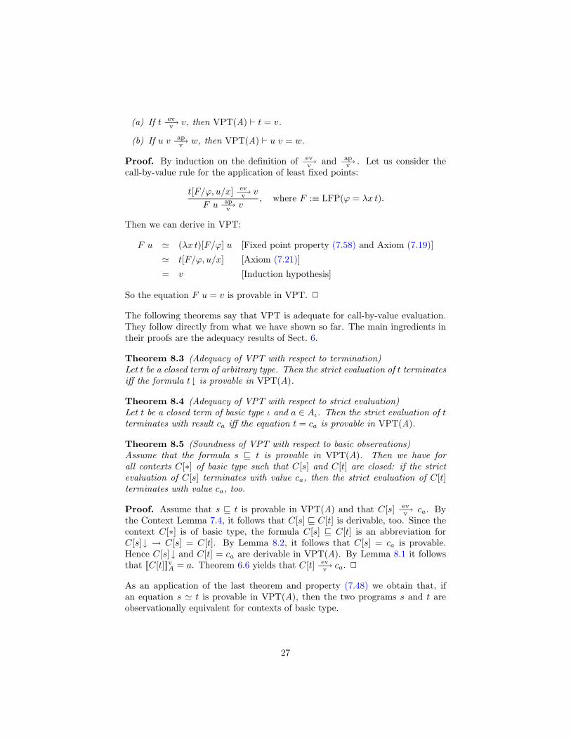
The following theorems say that VPT is adequate for call-by-value evaluation.They follow directly from what we have shown so far. The main ingredients intheir proofs are the adequacy results of Sect. 6.
Theorem 8.3 (Adequacy of VPT with respect to termination)Let t be a closed term of arbitrary type. Then the strict evaluation of t terminatesiff the formula t↓ is provable in VPT(A).
Theorem 8.4 (Adequacy of VPT with respect to strict evaluation)Let t be a closed term of basic type ι and a ∈ Aι. Then the strict evaluation of tterminates with result ca iff the equation t = ca is provable in VPT(A).
Theorem 8.5 (Soundness of VPT with respect to basic observations)Assume that the formula s v t is provable in VPT(A). Then we have forall contexts C[∗] of basic type such that C[s] and C[t] are closed: if the strictevaluation of C[s] terminates with value ca, then the strict evaluation of C[t]terminates with value ca, too.
Proof. Assume that s v t is provable in VPT(A) and that C[s] −→evv ca. By
the Context Lemma 7.4, it follows that C[s] v C[t] is derivable, too. Since thecontext C[∗] is of basic type, the formula C[s] v C[t] is an abbreviation forC[s]↓ → C[s] = C[t]. By Lemma 8.2, it follows that C[s] = ca is provable.Hence C[s]↓ and C[t] = ca are derivable in VPT(A). By Lemma 8.1 it followsthat [[C[t]]]vA = a. Theorem 6.6 yields that C[t] −→ev
v ca. 2
As an application of the last theorem and property (7.48) we obtain that, ifan equation s ' t is provable in VPT(A), then the two programs s and t areobservationally equivalent for contexts of basic type.
27

9 The logic of partial terms for call-by-name
The logic or partial terms for call-by-name, NPT(A), is obtained from the basiclogic of partial terms by adding the axioms ∃xτ¬x↓ for each type τ which saysthat there exist undefined objects for each type τ .
NPT(A) := BPT(A) + ∃xτ¬x↓.
Since [[∃xτ¬x↓]]nα = true, for arbitrary assigenments α ∈ I nA, the logic NPT(A)
is sound with respect to the truth-definition [[·]]n of Table 4.
Lemma 9.1 (Soundness of NPT) If NPT(A) ` A then [[A]]nα = true for allassignments α ∈ I n
A.
The following prinicples are derivable in NPT(A):
(9.1) ∃x (t ' x), for x /∈ FV(t).
(9.2) ∀xA(x)→ A(t), A(t)→ ∃xA(x)
(9.3) (λx t)s ' t[s/x]
(9.4) 〈s, t〉↓
(9.5) π1(〈s, t〉) ' s, π2(〈s, t〉) ' t
These principles are used for the interpretation of call-by-name evaluation inNPT.
Lemma 9.2 (Interpretation of call-by-name evaluation in NPT)
(a) If t −→evn v then NPT(A) ` t = v.
(b) If u t −→apn v then NPT(A) ` u t = v.
Proof. By induction on the definition of −→evn and −→ap
n . Let us consider the rulefor the lazy application of least fixed points:
t[F/ϕ, s/x] −→evv v
F s −→apv v
, where F :≡ LFP(ϕ = λx t).
Then we can derive in NPT:
F s ' (λx t)[F/ϕ] s [Fixed point property (7.58) and Axiom (7.19)]
' t[F/ϕ, s/x] [Unrestricted β-axiom (9.3)]
= v [Induction hypothesis]
So the equation F s = v is provable in NPT. 2
The main theorems which relate NPT to non-strict evaluation are the same asin the strict case. They follow directly from the previous results using compu-tational adequacy of Sect. 6.
28

Theorem 9.3 (Adequacy of NPT with respect to termination)Let t be a closed term of arbitrary type. Then the non-strict evaluation of tterminates iff the formula t↓ is provable in NPT(A).
Theorem 9.4 (Adequacy of NPT with respect to strict evaluation)Let t be a closed term of basic type ι and a ∈ Aι. Then the non-strict evaluationof t terminates with result ca iff the equation t = ca is provable in NPT(A).
Theorem 9.5 (Soundness of NPT with respect basic observations)Assume that the formula s v t is provable in NPT(A). Then we have for allcontexts C[∗] of basic type such that C[s] and C[t] are closed: if the non-strictevaluation of C[s] terminates with value ca, then the non-strict evaluation ofC[t] terminates with value ca, too.
A comparison of VPT and NPT
The main difference between NPT and VPT is that in NPT quantifiers rangeover possibly undefined objects, whereas in VPT they range over defined ob-jects only. So NPT is no longer a logic of definedness [7] and the question is,whether this could be changed. We do not think so. How could the axiom ofextensionality (7.32) for call-by-name be formulated without letting quantifiersrange over the object ‘undefined’? Under call-by-name two functions are equal,only if they agree on undefined arguments, too. For example, the functions
λx (x ? tt : tt) and λx tt
agree on defined arguments, but not on the argument ‘undefined’. Under call-by-name they are not considered as equal. Also in the definition of the ‘lessdefined’ relation (v) quantifiers have to range over the object ‘undefined’ in thecase of call-by-name (see Definition 7.1). Therefore we believe that a logic ofdefinedness for call-by-name does not exist.
A Appendix: Simultaneous least fixed points,Moschovakis’ formal language of recursionand program transformation
Moschovakis [18] introduces the Formal Language of Recursion (FLR), a formallanguage of terms with two semantics, a denotational semantics and an inten-sional semantics. He studies a calculus of reductions and equivalence for terms,formalizing compilation of terms into unique normal forms. He considers sideeffects and therefore the order of the evaluation of the arguments of a functionis relevant.
In this appendix, we show how BPT can be used to prove the soundnessof Moschovakis’ reduction calculus. We refer the reader to [18] for the exactdefinition of the reduction calculus. We only consider the two most important
29
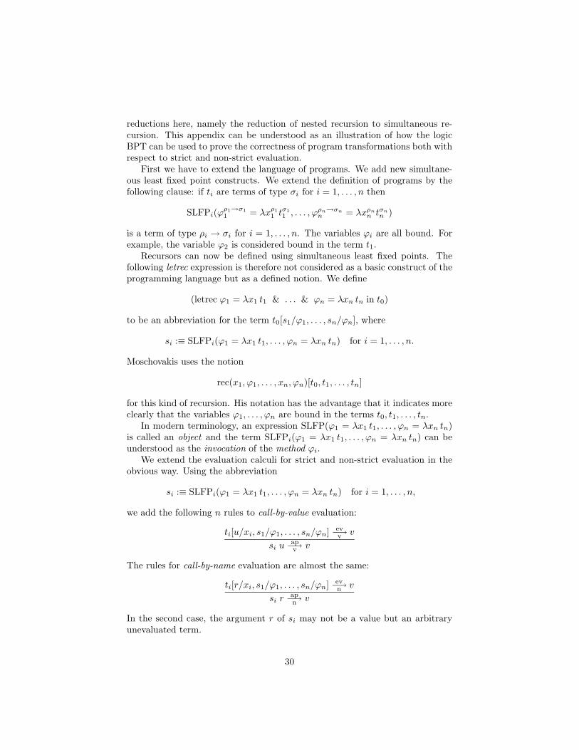
reductions here, namely the reduction of nested recursion to simultaneous re-cursion. This appendix can be understood as an illustration of how the logicBPT can be used to prove the correctness of program transformations both withrespect to strict and non-strict evaluation.
First we have to extend the language of programs. We add new simultane-ous least fixed point constructs. We extend the definition of programs by thefollowing clause: if ti are terms of type σi for i = 1, . . . , n then
SLFPi(ϕρ1→σ11 = λxρ1
1 tσ11 , . . . , ϕρn→σnn = λxρnn tσnn )
is a term of type ρi → σi for i = 1, . . . , n. The variables ϕi are all bound. Forexample, the variable ϕ2 is considered bound in the term t1.
Recursors can now be defined using simultaneous least fixed points. Thefollowing letrec expression is therefore not considered as a basic construct of theprogramming language but as a defined notion. We define
(letrec ϕ1 = λx1 t1 & . . . & ϕn = λxn tn in t0)
to be an abbreviation for the term t0[s1/ϕ1, . . . , sn/ϕn], where
si :≡ SLFPi(ϕ1 = λx1 t1, . . . , ϕn = λxn tn) for i = 1, . . . , n.
Moschovakis uses the notion
rec(x1, ϕ1, . . . , xn, ϕn)[t0, t1, . . . , tn]
for this kind of recursion. His notation has the advantage that it indicates moreclearly that the variables ϕ1, . . . , ϕn are bound in the terms t0, t1, . . . , tn.
In modern terminology, an expression SLFP(ϕ1 = λx1 t1, . . . , ϕn = λxn tn)is called an object and the term SLFPi(ϕ1 = λx1 t1, . . . , ϕn = λxn tn) can beunderstood as the invocation of the method ϕi.
We extend the evaluation calculi for strict and non-strict evaluation in theobvious way. Using the abbreviation
si :≡ SLFPi(ϕ1 = λx1 t1, . . . , ϕn = λxn tn) for i = 1, . . . , n,
we add the following n rules to call-by-value evaluation:
ti[u/xi, s1/ϕ1, . . . , sn/ϕn] −→evv v
si u −→apv v
The rules for call-by-name evaluation are almost the same:
ti[r/xi, s1/ϕ1, . . . , sn/ϕn] −→evn v
si r −→apn v
In the second case, the argument r of si may not be a value but an arbitraryunevaluated term.
30

The denotations [[si]]vα of the single components of a simultaneous recursionare given by the least simultaneous fixed points of the operators Γiα defined by
Γiα(f1, . . . , fn) := [[λxi ti]]vα f1ϕ1... fnϕn
for i = 1, . . . , n.
This means that ([[s1]]vα, . . . , [[sn]]vα) is the least n-tuple of functions (f1, . . . , fn)such that fi = Γiα(f1, . . . , fn) for i = 1, . . . , n. The denotations [[si]]nα in the typestructures An
τ are defined in the same way.Finally, we can formulate the axioms for SLFP in the basic logic of partial
terms. We do not include computational induction, since we do not need it inthis appendix. We only add the fixed point property (FIX) and the minimalityproperty (MIN) to BPT. These principles are:
si = (λxi ti)[s1/ϕ1, . . . , sn/ϕn] (FIX)
∀ϕ1, . . . , ϕn (n∧∧i=1
λxi ti v ϕi →n∧∧i=1
si v ϕi) (MIN)
where si is the term SLFPi(ϕ1 = λx1 t1, . . . , ϕn = λxn tn) for i = 1, . . . , n.In the rest of this appendix we will show the soundness of two of Moschovakis’
reduction rules with respect to BPT. The first theorem is Moschovakis’ rule R4.It is the reduction of nested recursion to simultaneous recursion.
Theorem A.1 If ψ does not occur free in the program r, then we can derivein BPT the following equation:
(letrec ϕ = λx r in (letrec ψ = λy s in t)) ' (letrec ϕ = λx r & ψ = λy s in t).
Proof. We use the following abbreviations:
a1 :≡ LFP(ϕ = λx r), a2 :≡ LFP(ψ = (λy s)[a1/ϕ]),
bi :≡ SLFPi(ϕ = λx r, ψ = λy s), for i = 1, 2.
By definition, we have
(letrec ϕ = λx r in (letrec ψ = λy s in t)) ≡ t[a1/ϕ, a2/ψ].
We also have
(letrec ϕ = λx r & ψ = λy s in t) ≡ t[b1/ϕ, b2/ψ]
Thus, if we can derive a1 = b1 and a2 = b2 we are done, since BPT proves
a1 = b1 ∧ a2 = b2 → t[a1/ϕ, a2/ψ] ' t[b1/ϕ, b2/ψ].
First we show that we can derive b1 v a1 and b2 v a2. By the closure ax-iom (7.35) for LFP(ϕ = λx r), we have (λx r)[a1/ϕ] v a1. Since ψ is not freein r, the term (λx r)[a1/ϕ] is the same as (λx r)[a1/ϕ, a2/ψ] and we thus obtain
(λx r)[a1/ϕ, a2/ψ] v a1.
31

Again by the closure axiom (7.35) but this time for LFP(ψ = (λy s)[a1/ϕ]), weobtain (λy s)[a1/ϕ][a2/ψ] v a2. Since ψ does not occur free in a1, we have
(λy s)[a1/ϕ, a2/ψ] v a2.
Now, we can apply (MIN) and obtain that b1 v a1 and b2 v a2.For the converse inequalities, we use (FIX) and obtain (λx r)[b1/ϕ, b2/ψ] v
b1. Since ψ is not free in r, we have (λx r)[b1/ϕ] v b1 and, by the minimizationaxiom (7.36), we obtain a1 v b1, and by antisymmetry (7.48), a1 = b1.
Again by (FIX) it follows that (λy s)[b1/ϕ, b2/ψ] v b2. By the substitutionproperty (7.56), we can derive
(λy s)[b1/ϕ, b2/ψ] = (λy s)[a1/ϕ, b2/ψ].
Since ψ /∈ FV(a1) the term (λy s)[a1/ϕ, b2/ψ] is the same as (λy s)[a1/ϕ][b2/ψ]and, by property (7.47), we obtain (λy s)[a1/ϕ][b2/ψ] v b2. By the minimizationaxiom (7.36), we obtain a2 v b2, and by antisymmetry, a2 = b2. 2
The second theorem corresponds to rule R5 of Moschovakis. It is called theBekivc-Scott principle. It is the reduction of iterated to simultaneous leastfixed point recursion.
Theorem A.2 If χ does not occur free in r, s or t, then we can derive in BPTthe following equation:
(letrec ϕ = λx (letrec ψ = λy r in s) in t)'
(letrec ϕ = λx s[χ x/ψ] & χ = λxλy r[χ x/ψ] in t)
Proof. We use the following abbreviations:
a2 :≡ LFP(ψ = λy r), a1 :≡ LFP(ϕ = λx (s[a2/ψ])),bi :≡ SLFPi(ϕ = λx s[χ x/ψ], χ = λxλy r[χ x/ψ]), for i = 1, 2.
Note, that x and ϕ may appear free in a2. They are, however, not free in a1.Since (letrec ψ = λy r in s) is an abbreviation for s[a2/ψ], we have by definitionthat
(letrec ϕ = λx (letrec ψ = λy r in s) in t) ≡ t[a1/ϕ].
Also by definition, we have
(letrec ϕ = λx s[χ x/ψ] & χ = λxλy r[χ x/ψ] in t) ≡ t[b1/ϕ].
Since BPT provesa1 = b1 → t[a1/ϕ] ' t[b1/ϕ],
it is sufficient to show that a1 = b1 is derivable in BPT. It turns out, that inorder to do this, we have to show that λx a2[a1/ϕ] = b2 is derivable in BPT,too.
32

We first show the inequalities b1 v a1 and b2 v λx a2[a1/ϕ]. We have
(λx s[χ x/ψ])[a1/ϕ, λx a2[a1/ϕ]/χ] ≡ (λx s[χ x/ψ])[λx a2/χ][a1/ϕ]
≡ (λx s[(λx a2) x/ψ])[a1/ϕ]
[Context Lemma 7.4] = (λx s[a2/ψ])[a1/ϕ]
[Axiom (7.35)] v a1.
In a similar way we obtain
(λy r[χ x/ψ])[a1/ϕ, λx a2[a1/ϕ]/χ] ≡ (λy r[χ x/ψ])[λx a2/χ][a1/ϕ]
≡ (λy r[(λx a2) x/ψ])[a1/ϕ]
[Context Lemma 7.4] = (λy r[a2/ψ])[a1/ϕ]
[Axiom (7.35)] v a2[a1/ϕ].
Using the monotonicity property (7.53) we obtain
(λxλy r[χ x/ψ])[a1/ϕ, λx a2[a1/ϕ]/χ] v λx a2[a1/ϕ].
Hence we can apply (MIN) and obtain b1 v a1 and b2 v λx a2[a1/ϕ].For the converse inequalities a1 v b1 and λx a2[a1/ϕ] v b2, we use (FIX).
We have(λxλy r[χ x/ψ])[b1/ϕ, b2/χ] v b2
and, by the definition of v, we obtain (λy r[b2 x/ψ])[b1/ϕ] v b2 x and (b2 x)↓.By the minimality principle (7.36), it follows that a2[b1/ϕ] v b2 x. Using thisinequation, we derive
(λx s[a2/ψ])[b1/ϕ] ≡ (λx s[a2[b1/ϕ]/ψ])[b1/ϕ]
[Context Lemma 7.4] v (λx s[b2 x/ψ])[b1/ϕ]
≡ (λx s[χ x/ψ])[b1/ϕ, b2/χ]
[(FIX)] v b1.
By the minimality principle (7.36), we obtain a1 v b1. For the sake of com-pleteness we mention that we now have a2[a1/ϕ] v a2[b1/ϕ] v b2 x andλx a2[a1/ϕ] v b2. 2
Concluding remarks
The main goal of this article was to explain two different operational interpre-tations of the same programs by different logics. We have started with a classof simply typed programs that contain least fixed-point recursion and ended upwith two logics. The first logic, VPT, is adequate for call-by-value evaluation,whereas the second one, NPT, is adequate for call-by-name evaluation. This isshown using methods from denotational semantics, mainly adequacy theorems
33

which relate the (given) operational semantics with the denotational semantics.Neither the programs nor the logics contain the constant ‘undefined’.
It is possible to prove the adequacy of VPT and NPT directly without usingdenotational semantics. The proof, however, is tedious, since it needs termmodels and a direct proof of the so-called Context Lemma for call-by-value andfor call-by-name evaluation.
The systems VPT and NPT are obtained both as extensions of a systemwhich we call the basic logic of partial terms (BPT). The basic logic of partialterms is useful, since its theorems are valid under call-by-value as well as undercall-by-name interpretation. It is, however, not clear what the exact semanticsof BPT is. It also not clear how complete BPT is, i.e. whether it proves alltheorems that are common to VPT and NPT.1
All logics are formulated “locally” for a fixed structure A and so the questionis: how complete are these logics when we interpret them over the class of allstructures of a given signature? Is there a restricted completeness theorem?
In order to formulate the results of this article in the same context, thepartial functions of the given first-order structure are strict. For the call-by-name interpretation, it would be more natural to allow non-strict functions,too. The call-by-name evaluation rules for such functions, however, are ratherawkward, because if we want to apply a built-in function f to a term t then it isnot clear, whether the term t has to be evaluated and if so, which componentsof the result (which is a lazy pair) have to be evaluated before f is called.
The programs studied in this article are pure without side effects. In thepresence of side effects the standard notion of definedness splits into a myriad ofnotions (always evaluating to a value, being operationally equivalent to a value,being a value, etc.) The question is therefore whether this work could be carriedout for programs that contain side effects, and if so, whether this helps clarifythe different notions of definedness.
If we fix a set of axioms T for the structure A, then several proof-theoreticquestions arise. What is the proof-theoretic strength of BPT(T )? What arethe fragments of BPT(T ) obtained by restricting the scheme for computationalinductions to certain classes of formulas? — In the case of natural numbers Nand Peano Arithmetic PA it can be shown that VPT(PA) as well as NPT(PA)have the same strength as PA, since it is possible to interpret them in PA byformalizing suitable term models. This shows that VPT and NPT are first-orderlogics, although their terms are higher-order.
1I am grateful to Reinhard Kahle for the following observation: The disjunctions
(∀xτ11 x1 ↓ ∧ . . . ∧ ∀xτnn xn ↓) ∨ (∃xτ11 ¬x1 ↓ ∧ . . . ∧ ∃xτnn ¬xn ↓)
are in general not provable in BPT although they are provable in VPT as well as in NPT. Ifwe add the disjunctions to BPT, then we can prove all theorems common to VPT and NPT.For assume that VPT ` A and NPT ` A. By the deduction theorem, it follows that thereexist types τ1, . . . , τn such that the formulas
(∀xτ11 x1 ↓ ∧ . . . ∧ ∀xτnn xn ↓)→ A and (∃xτ11 ¬x1 ↓ ∧ . . . ∧ ∃xτnn ¬xn ↓)→ A
are provable in BPT.
34
References
[1] M. Beeson. Foundations of Constructive Mathematics. Springer-Verlag, 1985.
[2] W. Clinger and J. A. Rees. The revised4 report on the algorithmic languageScheme. ACM LISP Pointers, 4(3), 1991.
[3] W. M. Farmer. A partial function version of Church’s simple theory of types.J. of Symbolic Logic, 55(3):1269–1291, 1990.
[4] S. Feferman. A language and axioms for explicit mathematics. In J. N. Crossley,editor, Algebra and Logic, pages 87–139, Berlin, 1975. Springer-Verlag, LectureNotes in Mathematics 450.
[5] S. Feferman. Logics for termination and correctness of functional programs. InY. N. Moschovakis, editor, Logic from Computer Science, pages 95–127, NewYork, 1992. Springer-Verlag.
[6] S. Feferman. Logics for termination and correctness of functional programs, II.Logics of strength PRA. In P. Aczel, H. Simmons, and S. S. Wainer, editors,Proof Theory, pages 195–225. Cambridge University Press, 1992.
[7] S. Feferman. Definedness. Erkenntnis, 43:295–320, 1995.
[8] L. M. G. Feijs and H. B. M. Jonkers. Formal Specification and Design, volume 35of Cambridge Tracts in Theoretical Computer Science. Cambridge UniversityPress, Cambridge, UK, 1992.
[9] M. J. Gordon, A. J. Milner, and C. P. Wadsworth. Edinburgh LCF. Springer-Verlag, Lecture Notes in Computer Science 78, Berlin, 1979.
[10] C. A. Gunter. Semantics of Programming Languages: Structures and Techniques.The MIT Press, Cambridge, Massachusetts, 1992.
[11] S. Hayashi and H. Nakano. PX: A Computational Logic. The MIT Press, Cam-bridge, Massachusetts, 1988.
[12] P. Hudlak, S. L. Peyton Jones, and P. Wadler. Report on the programming lan-guage Haskell, a non-strict purely functional language. ACM SIGPLAN Notices,27(5), 1992.
[13] C. B. Jones and K. Middelburg. A typed logic of partial functions reconstructedclassically. Acta Informatica, 31(5):399–430, 1994.
[14] J. Kuper. Partiality in Logic and Computation — Aspects of Undefinedness. PhDthesis, University of Twente, Dept INF, Enschede, The Netherlands, 1994.
[15] Z. Manna. Mathematical Theory of Computation. McGraw-Hill, New York, 1974.
[16] I. A. Mason and C. L. Talcott. Inferring the equivalence of functional programsthat mutate data. Theoretical Computer Science, 105:167–215, 1992.
[17] R. Milner, M. Tofte, and R. Harper. The definition of Standard ML. The MITPress, 1990.
[18] Y. N. Moschovakis. The formal language of recursion. J. of Symbolic Logic,54(4):1216–1252, 1989.
[19] D. Park. Fixpoint induction and proofs of program properties. In B. Meltzerand D. Michie, editors, Machine Intelligence, volume 5, pages 59–78. EdinburghUniversity Press, Edinburgh, 1969.
[20] L. C. Paulson. Logic and Computation: Interactive Proof with Cambridge LCF.Cambridge University Press, Cambridge, 1987.
[21] R. A. Platek. Foundations of Recursion Theory. PhD thesis, Stanford University,Stanford, CA, 1966.
35
[22] R. A. Pljuvskevivcus. A sequential variant of constructive logic calculi for normalformulas not containing structural rules. In V. P. Orevkov, editor, The Calculiof Symbolic Logic, 1, volume 98 of Proceedings of the Steklov Institute of Mathe-matics, pages 175–229. AMS Translations (1971), 1968.
[23] G. D. Plotkin. Call-by-name, call-by-value and the λ-calculus. Theoretical Com-puter Science, 1:125–159, 1975.
[24] J. G. Riecke. The logic and expressibility of simply-typed call-by-value andlazy languages. Technical Report MIT/LCS/TR-523, MIT, Cambridge, Mas-sachusetts, 1991.
[25] D. S. Scott. Identity and existence in intuitionistic logic. In M. P. Fourman,C. J. Mulvey, and D. S. Scott, editors, Applications of Sheaves, pages 660–696.Springer-Verlag, Lecture Notes in Mathematics 753, 1979.
[26] N. Shankar. Recursive programming and proving. Technical report, ComputerScience Laboratory, SRI International, Menlo Park, CA, 1989.
[27] R. F. Stark. Call-by-value, call-by-name and the logic of values. In D. van Dalenand M. Bezem, editors, Computer Science Logic CSL ’96: Selected Papers, pages431–445. Springer-Verlag, Lecture Notes in Computer Science 1258, 1997.
[28] A. S. Troelstra and D. van Dalen. Constructivism in Mathematics: an Introduc-tion. North-Holland, Amsterdam, 1988.
[29] D. A. Turner. An overview of Miranda. ACM SIGPLAN Notices, 21(12):158–166,1986.
[30] G. Winskel. The Formal Semantics of Programming Languages: an Introduction.The MIT Press, 1993.
36