REP1 00World Bank Reprint Series: Number 100 June 1970

Surjit S. Bhalla

Measurement Errorsand the PennanentIncome Hypothesis:Evidence from Rural India

Reprinted with permission from The American Economic Review, vol. 69, no. 3 (June 1970), pp. 295-307

Pub

lic D

iscl

osur

e A

utho

rized

Pub

lic D

iscl

osur

e A

utho

rized

Pub

lic D

iscl

osur

e A

utho

rized

Pub

lic D

iscl

osur

e A

utho

rized

Pub

lic D

iscl

osur

e A

utho

rized

Pub

lic D

iscl

osur

e A

utho

rized

Pub

lic D

iscl

osur

e A

utho

rized

Pub

lic D

iscl

osur

e A

utho

rized

Measurement Errors and the Permanent IncomeHypothesis: Evidence From Rural India

By SURJIT S. BHALLA*

The traditional, or Keynesian, consumption The above two questions have been exten-hypothesis postulated that (a) current income sively investigated since the publication ofwas a prime determinant of consumption; and Friedman's theory two decades ago.' Nev-(b) that the average propensity to consume ertheless, with one exception, all these testsdeclined with income. This hypothesis was (including Friedman's) have been indirectrejected by Milton Friedman's permanent and nonrigorous. The exception was an inge-income hypothesis (PIH) which contended nious study by Nissan Liviatan, who usedthat (a) permanent income, and not current two-year panel Israeli data to test the PIH,income, was the relevant determinant of and, in particular, the proportionality hy-consumption; and (b) that permanent con- pothesis.4 His study, however, suffered from asumption was proportional to permanent major drawback in that it failed to accountincome (the proportionality hypothesis).' for the bias caused by common measurement

This paper attempts to test (and distinguish errors in consumption and income. This paperbetween) the two theories. Answers to two extends Liviatan's analysis by explicitlyquestions are sought: How important is the allowing for the presence of measurementcurrent income-permanent income distinc- errors in all the variables-income, consump-tion; and is the proportionality hypothesis, an tion, and saving. The empirical estimation ofimportant and controversial aspect of Fried- the variances of these errors (source of bias) isman's theory, valid? The resolution of the possible due to the availability of independentformer question has important implications estimates of consumption, savings, andfor the understanding of habit and lags in income.5 The data base is a three-year panelconsumption behavior and the efficacy of survey, conducted by the National Council ofshort-run macro-economic policies. The valid- Applied Economic Research (NCAER), Newity of the proportionality hypothesis has an Delhi, of 4,118 households in rural India.important bearing on the recently popular (See Appendix A for description of data andcontroversy regarding the tradeoff between definitions of variables.)growth and equity in developing countries.2 The incorporation of error variances in the

*World Bank. This is a shortened version of a paper therefore growth. (This is predicated on the assumptionwhich was written while I was a recipient of a Rockefeller that growth in less developed countries (LDCs) isPost-Doctoral Fellowship at the Rand Corporation The constrained by a lack of finance rather than of investmentfinancial support is gratefully acknowledged. I would like opportunities.) Thus, the PIH contends that there is noto thank William Rogers for helpful discussions, Thomas tradeoff between redistribution (equity) and growth.Mayer and Charles E. Phelps for comments on an earlier 3An excellent summary and interpretation of the volu-draft, and David Harrison for research assistance. The minous literature on consumption behavior is containedviews expressed in this paper are mine alone. in Thomas Mayer's book.

'Analogous conclusions are reached by the Modigliani- 4 Friedman accepted the compelling logic of Liviatan'sBrumberg life cycle hypothesis (LCH) of consumption tests and stated that " . . if these [Liviatan's] resultsbehavior. The two theories, LCH and PIH, use different should be confirmed for other bodies of data, they wouldempirical methods but employ a common theoretical constitute relevant and significant evidence that themodel of consumer behavior. The empirical techniques elasticity of permanent components is less than unity [theused in this paper apply directly to Friedman's formula- proportionality hypothesis]" (1963a, p. 63).tion of the theory. Hence, the emphasis is on testing the 5 These independent estimates allow for two measuresPIH. of consumption-direct consumption and residual con-

21f, as the proportionality hypothcsis implies, the sumption (income minus savings). This "excess" ofpropensity to consume permanent income is independent information is what makes the estimation of error vari-of the level of permanent income, then redistribution ances possible. See Section 11 (and Appendix B) forpolicies will be neutral with respect to savings, and details of methodology.

295

296 THE AMERICAN ECONOMIC REVIEW JUNE 1979

analysis, a unique aspect of this study, insures (2a) Z* = Z' + Z"that unlike Liviatan's tests, the tests of the (2b) Z Z* + Z° Z = Y CPIH in this paper are theoretically correct (and most rigorous to date. Further, account- The PIH assumes that the transitorying for errors allows for the estimation of components are independent of the perma-unbiased parameters of the Keynesian con- nent values, and each other, i.e.,sumption function and makes possible a validcomparison with the PIH. (3) cov (C', C") = cov (Y', Y")

The plan of the paper is as follows. Section cov (C", Y") = 0I presents a version of the PIH which isgeneralized to include the presence of pure Analogous to (3), it may be assumed thatmeasurement errors. Estimates of these error measurement errors per se are not correlatedvariances, as well as the uncorrected and with the true values, or with each other:'corrected parameters of a Keynesian con-sumption function, are also presented. The (4) cov (C*, C) = cov (Y*, Y°) =

"horizon," a crucial parameter in the PIH, is cov (Co, Y0) = 0defined, estimated, and corrected for mea-surement errors in Section 11. A test of the Apart from equations (2) and (3), a thirdproportionality hypothesis, and a comparison relationship is postulated by the PIH; namely,of the PIH with the standard Keynesian that the permanent components are systemat-model, is presented in Section 111. ically related to each other, c' = ky', where k

is assumed to be dependent on interest rates,tastes, compositon of wealth, etc., but inde-

1. A Generalized Version of the PIH pendent ofy'. This assertion implies a unitaryelasticity between the permanent compo-

An important feature of this study is the nents, i.e.,distinction it makes between measurementerrors proper, and the "measurement error"Ccaused by the presence of transitory terms in As is well known, estimation of the stan-the measured variables. Accounting for this dard Keynesian function (c = a + by or C =distinction is necessary, and crucial, for a A + BY) in the absence of measurementvalid test of the PIH. errors yields a downwardly biased estimates

If measurement errors in income y, of the permanent elasticity, n':consumption c, and savings s are present, thena generalized version of the permanent (6) i7 = var Y' / (var Y' + var Y")income hypothesis would be < 7' =

(la) z* = z' + z" Allowance for measurement errors in Ybiases

(Ib) z z* + z°, z =y,c,s

where z* represents the true value, z'(z") assumption results in a point estimate of the marginal

represent the permanent (transitory) terms, z propensity to consume; the latter in a point estimate ofrepresents the measured value and z° the the consumption elasticity. Though both models aremeasurement error. Analogously, the vari- discussed, the development of the model is outlined in its

ables can be expressed in logarithmic logarithmic variant. Note that equation (2) does not:6 contain an equation for savings, which can be negative for

terms: an individual household.7The assumption that the measurement errors are not

6Lowercase letters represent natural numbers; upper correlated with each other needs to be qualified. Somecase letters represent the logarithm (log) of a number. items are common to consumption and income (forEquation (I) (arithmetic model) is implied by the example, housing) whereas others are common to savingsassumption that transitory terms are additively distrib- and income (nonmonetized investment). The magnitudesuted; if the variables are multiplicatively distributed (i.e., of these covariances are likely to be relatively small andy = y'y") then a logarithmic model results.-The former are therefore ignored.

VOL. 69 NO 3 BHALLA. PERMANENT INCOME HYPOTHESIS 297

downward the true measured elasticity ??*, as savings can be achieved ex post by assumingwell: that each household underestimates its

(6') ~* > ~ 'c~ (C, Y) /consumption by a constant proportion a.(6') 77 * > 77 cov (C, Y) /Thus, direct consumption c is no longer equal

(var Y* + var Y°) to c* + co, rather, c = ac* + co, whereThe relative magnitudes of var Y" and 0 < a < 1. If s is a "true" measure of

var Y°are unknown; lack of knowledge of the aggregate savings, then a = E(c)/[E( y) -error variance var Yocan negate any compar- E(s)].ison between the two consumption theories; Given the ex post equality between c andthat is, a comparison of the permanent elas- c_, and the value of a, a "method of moments"ticity 77' with the traditional elasticity ij*. approach can be used to derive the variances,Further, a valid test of whether s7' is cqual to var y°, var c°, and var so. (A key equation inunity cannot be conducted. Fortunately, given the derivation is the identity between truecertain assumptions, the magnitude of var Y° valuesy* = c* + s*.) Two different assump-(and error variances in savings and consump- tions about the distribution of the errors aretion) can be estimated. considered: (a) errors affect true values addi-

A maintained and general assumption in tively (arithmetic model, equation (Ib)); andthis paper is that measurement errors (co, s°, (b) errors affect true values proportionallyand y°) are independent of the true values, (multiplicative model, equation (2b)). Theseand have a zero mean. Thus, E(z) = E(z*) two assumptions, though not exhaustive,and E(c) = E( y) - E(s), where E( ) is the cover a wide rangc of possibilities. Of the two,expectation operator. Thus, the aggregate it is likely that the multiplicative assumptionestimates of c and its residual estimate, is more reasonable, that is, it is more likelyc,, c, = y - s (alternatively s and s,), should that rich and poor households make the samebe approximately equal. Such is not the case. proportional error, X percent, rather than theThe saving rates for the three years-1968- same absolute error.69, 1969-70, and 1970-71-are -0.6, 4.2, The solution of error variances is straight-and 5.4 percent, respectively, for the direct forward for the arithmetic model; for themeasure, and 13.6, 14.6, and 16.3 percent, more realistic multiplicative model, the meth-respectively, for the residual measure s,. odology is much more involved. The difficulty(s, = y - c where c is (presumably) under- arises primarily because the crucial identitystated.) The difference between s and s, is too y* = C* + s* does not exist in its (multipli-large to be accounted for by the omission of cative) logarithmic transformation, i.e..certain savings (cash and jewelry) from s. The Y* t C* + S*. Nevertheless, an appro-explanation is more likely in terms of the priate procedure exists. The solutions areparticular aims of the survey-detailed outlined in Appendix B. The expressions forassessment of investment patterns (and there- the income error variances for the two modelsfore, s) was one of the major goals of the are9survey; enumeration of consumption expendi- 7 -Itures (and therefore s,) was not. Thus, it is (7a) vary = vary-cov (s,y) -

likely that a certain fraction of consumption cov (c, y)expenditures was systematically excluded (7b) var Y° = In (I + var M)from enumeration and therefore s, > s.Comparison with published national esti- where var M =mates also indicates that s at the aggregate a var y - cov (c, y) - a cov (s, y)level is a more accurate measure of ruralsavings.8 a [E( y)] 2 + cov (c, y) + a cov (5, y)

An equality between the two estimates of9 Appendix B also contains expressions for errors in

savings and consumption. Since the primary concern is'See the author for a detailed discussion of various with errors in the independent variable, income, only

savings cstimates, and a comparison of s and s,. these are discussed in the rest of the paper.

298 THE AMERICAN ECONOMIC REVIEW JUNE 1979

TABLE I-ERROR VARIANCES AND RELATED STATISTICS

Year I Year 2 Year 31968-69 1969-70 1970-71

Mean Income, Rs. 4544 4732 4988Alpha E(c)/I[E(y) -E(s)] .804 .850 .860Direct Consumption, c

APC .778 .759 .741MPC,,B .39 .49 .47a (adjusted by a) .48 .58 .5571 (arithmetic model) .50 .65 .63?I (log model) .53 .71 .73

Residual Consumption, c,APC .97 .89 .86, .91 .70 .65in (arithmetic model) .94 79 .7671 (log model) .88 .80 .80

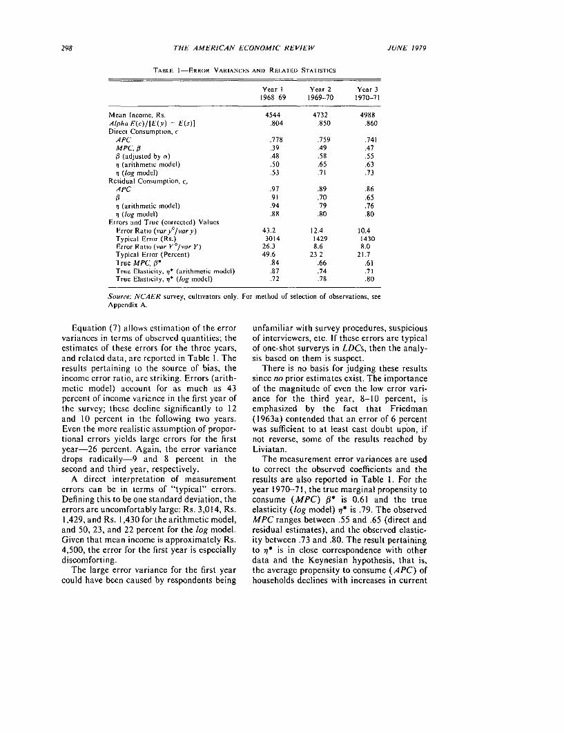
Errors and True (corrected) ValuesError Ratio (vary°/vary) 43.2 12.4 10.4Typical Error (Rs.) 3014 1429 1430Error Ratio (var Yo/var Y) 26.3 8.6 8.0Typical Error (Percent) 49.6 23 2 21.7True MPC, fl* .84 .66 .61True Elasticity, i7* (arithmetic model) .87 .74 .71True Elasticity, 77* (log model) .72 .78 .80

Source: NCAER survey, cultivators only. For method of selection of observations, seeAppendix A.

Equation (7) allows estimation of the error unfamiliar with survey procedures, suspiciousvariances in terms of observed quantities; the of interviewers, etc. If these errors are typicalestimates of these errors for the three years, of one-shot surverys in LDCs, then the analy-and related data, are reported in Table 1. The sis based on them is suspect.results pertaining to the source of bias, the There is no basis for judging these resultsincome error ratio, are striking. Errors (arith- since no prior estimates exist. The importancemetic model) account for as much as 43 of the magnitude of even the low error vari-percent of income variance in the first year of ance for the third year, 8-10 percent, isthe survey; these decline significantly to 12 emphasized by the fact that Friedmanand 10 percent in the following two years. (1963a) contended that an error of 6 percentEven the more realistic assumption of propor- was sufficient to at least cast doubt upon, iftional errors yields large errors for the first not reverse, some of the results reached byyear-26 percent. Again, the error variance Liviatan.drops radically-9 and 8 percent in the The measurement error variances are usedsecond and third year, respectively. to correct the observed coefficients and the

A direct interpretation of measurement results are also reported in Table 1. For theerrors can be in terms of "typical" errors. year 1970-71, the true marginal propensity toDefining this to be one standard deviation, the consume (MPC) 0* is 0.61 and the trueerrors are uncomfortably large: Rs. 3,014, Rs. elasticity (log model) q* is .79. The observed1,429, and Rs. I ,430 for the arithmetic model, MPC ranges between .55 and .65 (direct andand 50, 23, and 22 percent for the log model. residual estimates), and the observed elastic-Given that mean income is approximately Rs. ity between .73 and .80. The result pertaining4,500, the error for the first year is especially to 7* is in close correspondence with otherdiscomforting. data and the Keynesian hypothesis, that is,

The large error variance for the first year the average propensity to consume (APC) ofcould have been caused by respondents being households declines with increases in current

VOL. 69 NO. 3 BHALLA: PERMANENT INCOME HYPOTHESIS 299

income. If the PIH is mostly true, then the data. Assumptions (additional to equationspermanent elasticity should be significantly (1)-(5)) are necessary, but since these arehigher than 77* and (perhaps) equal to unity. identical to those made by Friedman, the testsBut before sn' can be computed, it is necessary are within the spirit (if not the letter) of thefor the horizon to be estimated. This crucial PIH. In particular, it is assumed that theparameter can also be biased by measurement permanent component of income changes (iferrors; uncorrected and corrected estimates of at all) in a systematic manner from year tothe horizon are presented in the next year. The systematic nature of change issection. either "that permanent components maintain

the same ratio to the mean of the group in11. The Horizon different years" (mean assumption), or "that

the fraction of the total variability contrib-The proper length of the horizon has been a uted by the permanent components is the

contentious issue in the literature on same in successive years" (variability as-consumption theory.'" Part of the disagree- sumption), (Friedman, 1957, p. 184).ment can be attributed to the fact that Fried- For the log model, mean assumption, theman offers two definitions of the horizon elasticity of incomes for any two years of thewithout attempting to show any equivalence survey (indicated by the subscripts i and j),between the two. One definition is derived isfrom considerations of wealth and its conver-sion into permanent income. Accordingly, if (8) ny1yj = cov (Y,, Y,)/var Y,the subjective discount rate is r, "the horizon = cov (Y,' + Y7 + Y°,can then be defined as l/r, or 'the number of Y, + Y,years purchase' implied by the discount rate" + Y,°)/var (Y, + Y" + Y°)(Friedman, 1963b, p.7). The second defini-tion is directly related to the statistical formu- If Y' is systematically related to Y, (forlation of the PIH and concerns itself with the example, y' Xy= or Y,' = r + Y,), thenseparation of an income stream into itspermanent and transitory components; "the (8') 7 Y,Y= coy (P + + Y" + Y,length of time a factor must affect income Y, + Y,' + Y,°)/var Yjbefore it is regarded as permanent is a =(var Y0 + AY Y +AY°Y°)var Ymeasure of the length of the horizon" (Hol- v Y'' ' '/abrook, p.750). According to the latter defini- where A's represent the respective covariancestion, a two-year horizon would imply that the (i.e., AY" Y7 ' = cov (Y,', Y,')). If thesetransitory terms for the two years are not covariances are assumed to be zero, then (8')correlated. Analogously, "suppose the horizon reduces towere three years. Some factors would then be (regarded as transitory even though they (9) 7yyj = var Y,/var Y,affected income in two years, so transitory Equation (9) is exactly as that obtained forterms in successive years would be correlated, the elasticity of consumption with respect tothough in years separated by a year they measured income, - (equation (6) ). Analo-would be uncorrelated" (Friedman, 1957, gously, it can be shown that the correlation ofp. 196). incomes p,,} is the measure comparable to -1

A direct estimate of the second definition under the variability assumption (see Fried-of the horizon can be achieved with NCAER man, 1957, p. 184):

(9') py,yj = cov(Yi, Yj)/"Friedman contends that the horizon is three years. (vr Y )5(var Y )-5}

Though Khan Mohabatt and Evangelos Simos support ( (v , }Friedman, Robert Holbrook asserts that the horizon isconsiderably shorter. Michael Landsberger, however, This imples i = cov(C, Y,)/var Y,. Thesefinds evidence in support of a three-year horizon with equivalences" can now be used to test for theIsraeli data. length of the horizon. If transitory incomes

300 THE AMERICAN ECONOMIC REVIEW JUNE 1979

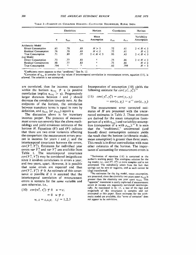
TABLE 2-EVIDENCE ON CONSUMER HORIZON-CULTIVATOR HOUSEHOLDS, RURAL INDIA

Elasticities Horizon Correlations Horizon

Mean Variability7 77Y2Y3 '?YIY3 Assumption pY2Y3 PVIY3 Assumption

Arithmetic ModelDirect Consumption .63 .70 .69 H > 3 .72 .61 2 < H < 3Residual Consumption .76 .70 .69 H < 2 .72 .61 H < 2True Consumption .71 .89 .57 2 < H < 3 .93 .43 2 < H < 3

Log ModelDirect Consumption .73 .77 .83 .75 .66 2 < H < 3Residual Consumption .80 .77 .83 .75 .66 H < 2True Consumption .794 b b b .82 .799 H = 3

'Coefficients move opposite to that "predicted." See fn. 12.bCorrection of iy, is complex for log values if intertemporal correlation in measurement errors, equation (I1), is

allowed. The solution is not attempted.

are correlated, then for incomes measured Incorporation of assumption (10) yields thewithin the horizon 7Y,Yj =t ?I (a positive following estimate for cov(y,, y,):"correlation implies 77,jj > 77). Progressively O 0larger distances between i and j should (11) cov(y ,y,0) = cov(y,,y,)decrease the correlation towards zero. At the - cov(s,, y) - a-' cov(c,, y,)endpoints of the horizon, the correlationbetween transitory terms is equal to zero by The measurement error corrected esti-definition, and i7tjrJ (or p,,,) equals 77. mates of H are presented with the uncor-

The discussion above is for transitory rected estimates in Table 2. These estimatesincomes proper. The presence of measure- are derived for the mean assumption (com-ment errors can severely bias the above meth- parison of 71 with -qy,y,) and variability assump-odology and yield erroneous estimates of the tion (comparison of 7 with p"Y,).l2 It is seenhorizon H. Equations (8') and (9') indicate that the "traditional," uncorrected (andthat there are two error variances affecting biased) direct consumption estimate yieldsthe comparison: the measurement errors pres- the result that the horizon (arithmetic model,ent in incomes for years i and j; and the mean assumption) is greater than three years.intertemporal covariance between the errors, This result is in direct contradiction with mostcov(Y?,, Y,). Estimates for individual year other estimates of the horizon. The impor-errors var Y,° and var Y5° are available from tance of accounting for measurement errors isTable 1. The intertemporal covariancecov(Y?, Y9) may be considered insignificant "Derivation of equation (11) is contained in thesince it involves correlations in errors a year, author's working paper. The analogous solution for the

and two years, apart. However, it is possible emodel, i.e, cov( ex Yit) arises from the fact thatthat some errors are repeated and thus savings can be zero or negative, and as such cannot becov(Y9°, Y°) :f 0. An estimate of this covar- (log) transformed.iance is possible if it is assumed that the '2 No estimates for the log model, mean assumption,

tt al correlation of measurement are presented, since the elasticity two years apart i7 y, isintertemporal correlatlon ol measurement greater than the elasticity one year apart 17YM. Thiserrors is nonzero for the same variable and "opposite" movement is easily explained If measurementzero otherwise, i.e., errors in income are negatively correlated intertempo-

rally. As mentioned in fn. II, a test of the sign and(10) COV(Wj°, ) 0 w =z; magnitude of this covariance is complex and not

0 w zattempted in this paper. Since estimates for the arith-metic model are available, this "error of omission" does

w, z = c,s,y; i,j = 1,2,3 not appear to be restrictive.

VOL. 69 NO. 3 BHALLA: PERMANENT INCOME HYPOTHESIS 301

emphasized by the fact that correction for between the transitory terms and measure-these errors reduces the estimate of H to ment errors. And if the A's are zero, then 77xbetween two and three years. The variability reduces to the unitary permanent elasticityassumption, log model, yields an estimate of estimate i7'.

H equal to three years. All other estimates Liviatan used the instrumental variable(corrected and uncorrected) place H to be less technique with two-year Israeli data andthan three years. concluded that 11X was less than unity. His

The "corrected" result that the upper instruments were the estimates of consump-bound for the horizon is three years is used in tion and income of the "other" year. Unfortu-the next section to conduct strong tests of two nately, his estimate of consumption was acomponents of the PIH: (a) how much larger residual estimate (i.e., c, = y - s) andis the permanent elasticity i7' from the cor- therefore common measurement errors wererected elasticity 71* (i.e., how important is the present in c and y. Further, two-year datadistinction between permanent and transitory meant (if H > 2) that the A's were nonzero.income), and (b) is the proportionality hy- Consequently, Liviatan's results were ques-pothesis valid, i.e., is i7' = 1. The tests of the tioned by Friedman. Nevertheless, Liviatan'shorizon itself were based on the assumption tests were accepted by Friedman, who statedthat i7' is equal to unity. However, a "logical that "it is most desirable that his [Liviatan's]trap" is avoided if one notes that the method analysis be applied to data not marred byof estimating H-comparison of 77,,, and common errors of measurement in incomen-yields an upper bound of the horizon if the and consumption. It would further be highlypermanent consumption-income elasticity is desirable to have such data spanning at least aless than unity. Since the bias is in the "right" three-year period so that income anddirection, the rigorous tests outlined next are consumption for one year could be used as anvalid. instrumental variable for a year at least two

years later or earlier" (1973b, p. 63).III. Estimates of the Permanent Income Model Given the result that the upper bound for

the horizon is three years, the three-yearA generalized cxpression for the measured NCAER panel data fulfills all the require-

consumption elasticity, with PIH assump- ments for a valid test. Further, the availabilitytions, is of separate estimates for consumption and

saving suggests the presence of six proper77 = var Y'/(var Y' + var Y" instruments: income and two consumptions

+ var Y°) < 7* < = I definitions for year I (c and c,) for eachdefinition of consumption for year 3. If the

The fact that it is the presence of errors PIH is correct, each instrument should yield(Y" and Y°) in Y which causes 77' to be an unbiased unitary permanent elasticity.downwardly biased suggests the use of an This is only possible if all the A's are zero. Theinstrumental variable for Y. If this variable is correlation amongst transitory terms is zerorepresented by X, then the (instrument) (by definition) for variables two years apart.'3

consumption elasticity is The intertemporal measurement error corre-x = cov(C, X)/cov( Y, X) lations, however, may be nonzero. If so, then

the use of first-year consumption C, (sub-If the proportionality hypothesis is valid scripts denote years) on a regression involving(C' = K + Y'), then( 12) x = (cov (Y', X) "3The results of Tablc 3 are for a definition of

(12) .X = (cov( Y', X') consumption which excludes durabic expenditurcs. This+ AC"X" + AC 0x 0)/ exclusion should minimize any possible correlation

between the transitory components All the tests of Table(cov( Y', X') + AY"C" + A Y X0) 3 were reestimated for a definition of consumption which

included durable expenditure; virtually no difference waswhere the A's represent the covariances observed in the results.

302 THE AMERICAN ECONOMIC REVIEW JUNE 1979

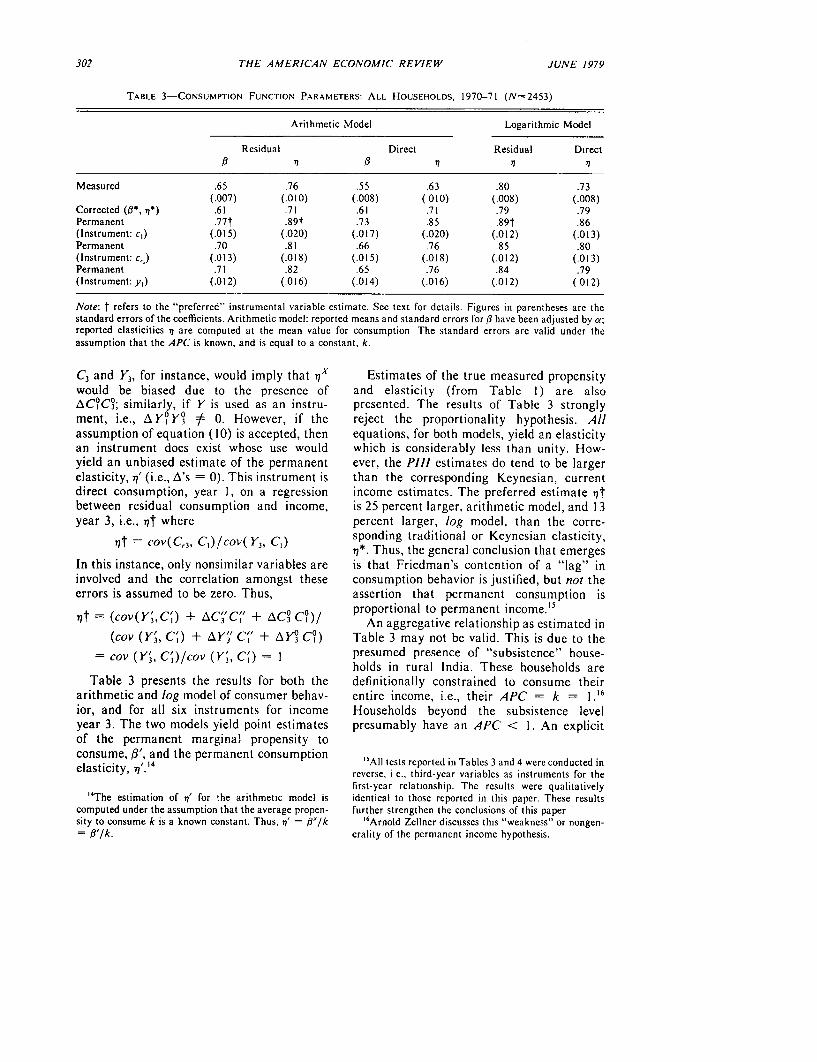
TABLE 3-CONSUMP'TION FUNCTION PARAMETERS: ALL HOUSEHOLDS, 1970-71 (N-2453)

Arithmetic Model Logarithmic Model

Residual Direct Residual Direct0 1~ ~~~~7 7 7 1771

Measured .65 .76 .55 .63 .80 .73(.007) (.010) (.008) (010) (.008) (.008)

Corrected (0*, 1*) .61 .71 .61 .71 .79 .79Permanent .77t .89t .73 .85 .89t .86(Instrument: c,) (.015) (.020) (.017) (.020) (.012) (.013)Permanent .70 .81 .66 .76 .85 .80(Instrument: c,,) (.013) (.018) (.015) (.018) (.012) (.013)Permanent .71 .82 .65 .76 .84 .79(Instrument: y,) (.012) (.016) (.014) (.016) (.012) (012)

Note: t refers to the "preferred" instrumental variable estimate. See text for details, Figures in parentheses are thestandard errors of the coefficients. Arithmetic model: reported means and standard errors for , have been adjusted by a;reported elasticities 71 are computed at the mean value for consumption The standard errors are valid under theassumption that the APC is known, and is equal to a constant, k.

C3 and Y3, for instance, would imply that i7 Estimates of the true measured propensitywould be biased due to the presence of and elasticity (from Table 1) are alsoAC,OC03; similarly, if Y is used as an instru- presented. The results of Table 3 stronglyment, i.e., AY,°YO3 7 0. However, if the reject the proportionality hypothesis. Allassumption of equation (10) is accepted, then equations, for both models, yield an elasticityan instrument does exist whose use would which is considerably less than unity. How-yield an unbiased estimate of the permanent ever, the PIH estimates do tend to be largerelasticity, 1' (i.e., A's = 0). This instrument is than the corresponding Keynesian, currentdirect consumption, year 1, on a regression income estimates. The preferred estimate 7tbetween residual consumption and income, is 25 percent larger, arithmetic model, and 13year 3, i.e., i7t where percent larger, log model, than the corre-

t = cov(C,3, C)/cov( Y CO) sponding traditional or Keynesian elasticity,73*. Thus, the general conclusion that emerges

In this instance, only nonsimilar variables are is that Friedman's contention of a "lag" ininvolved and the correlation amongst these consumption behavior is justified, but not theerrors is assumed to be zero. Thus, assertion that permanent consumption is

t ov(Y3,C') ic'qC"C" + AC, C° proportional to permanent income.'51 -(cov( 3, 1) 3 1 3 1)/ An aggregative relationship as estimated in(cov (Y', Cl) + AY', C"' + AYo° Co) Table 3 may not be valid. This is due to the

= cov (Y'3, C)/cov (Y', C) = I presumed presence of "subsistence" house-3 I 3 holds in rural India. These households are

Table 3 presents the results for both the definitionally constrained to consume theirarithmetic and log model of consumer behav- entire income, i.e., their APC = k = 1 6

ior, and for all six instruments for income Households beyond the subsistence levelyear 3. The two models yield point estimates presumably have an APC < 1. An explicitof the permanent marginal propensity toconsume,,' and the permanent consumption ,cnsue . ' ad te p4 eAll tests reported in Tables 3 and 4 were conducted inelasticity, 17 reverse, i e., third-year variables as instruments for the

first-year relationship. The rcsults were qualitatively"'The estimation of i7' for the arithmetic model is identical to those reported in this paper. These results

computed under the assumption that the average propen- further strengthen the conclusions of this papersity to consume k is a known constant. Thus, 7' = ,3'/k '6 Arnold Zellner discusses this "weakness" or nongen-= R'/k. erality of the permanent income hypothesis.

VOL. 69 NO 3 BHALLA PERMANENT INCOME HYPOTHESIS 303

TABLE 4-CONSUMPTION FUNCTION PARAMETERS

Arithmetic Model Logarithmic Model

Residual Direct Residual Direct

Subsistence Households (N = 1146)Measured .86 .85 .84 .83 .83 .80

(.012) (.012) (.014) (.013) (.013) (014)Corrected ((3*, '7*) .86 .86 .86 86 .82 82Permanent 1.01t .997t 1 03 1.03 1.03t 1 04(Instrument: c,) (.026) (.026) (.030) (.027) (.029) (.040)Permanent .97 .96 .97 .96 .96 .95(Instrument: c,,) (.025) (025) (.028) (.026) (.029) (.03)Permanent .99 .98 .99 .98 .97 .94(Instrument: y,) (.024) (.024) (.027) (.025) (.030) (.031)

Nonsubsistence Households (N = 1307)Measured .62 .76 .50 62 .80 .72

(.011) (.014) (.013) (.013) (.013) (014)Corrected (fl*, 77*) .57 .70 .57 .70 .79 .79Permanent .76t .94t .74 .91 92t 92(Instrument c,) (.027) (.033) (.032) (.033) ( 026) (.029)Permanent .68 .84 .66 .82 .88 .88(Instrument! c,,) (.025) (.031) (.030) (.031) (.032) (.035)Permanent .69 .85 .66 .81 .88 87(Instrument: y,) (.023) (.028) (.028) (.031) (.028) (.03)

Note: See Table 3.

dependence between the APC and the perma- holds, the unbiased permanent elasticity isnent income level is therefore built into the very close to one, and never significantlymodel, and an elasticity less than one is the different from one. The most interestingexpected result. Thus, a test of the proportion- result regarding these households is not thatality hypothesis is inappropriate. the elasticity is equal to one, but rather that

Identification of a subsistence level, how- the permanent marginal propensity to con-ever, is difficult. The subject has been sume income is not different from one. Thesediscussed at length in the Indian literature results conform very well to any prior expec-and the consensus seems to be that an annual tation about subsistence level behavior.income of Rs. 450 per capita, 1970-71 prices Subsistence households, if properly defined,(corresponding to Rs. 15-20 per month, should have a marginal propensity equal to1960-61 prices) adequately describes the one. Indeed, my results suggest an alternativesubsistence level. If it is assumed that three- definition of a subsistence level; in particular,year average per capita income ya adequately that such a level (or range) is one after whichreflects permanent status, then Ya § Rs. 500 the permanent marginal propensity becomesshould conservatively separate households less than one.into subsistence-nonsubsistence categories. If The results for nonsubsistence householdsconsumption functions are estimated for each represent the strongest possible test of thegroup separately, then the prior expectation PIH. The a priori dependence between thewould be that (a) ,l' for subsistence house- propensity to consume and permanent incomeholds is unity (they are constrained to has been "purged" from the data. The results,consume their entire income) and (b) s7' for however, are not favorable to the proportion-nonsubsistence households is also unity, if the ality assumption. For all instruments (arith-PIH is valid. metic and logarithmic models), the elastici-

Table 4 contains the results for the two ties are significantly less than one at the Iclassifications. For subsistence level house- percent level of confidence. These elasticities

304 THE AMERICAN ECONOMIC REVIEW JUNE /979

range from .87 to .92, log model. The result that the APC and MPC decline withpreferred result 71t yields 71' equal to .92 which increases in current income. The observedis significantly less than unity, but is also decline of MPC out of permanent incomeconsiderably larger than the corrected suggests that income redistribution policiesKeynesian elasticity, 71* = .79. are likely to have, ceteris paribus, a negative

impact on the supply of household savings,IV. Conclusions and consequently growth, in the LDCs.

The importance of the bias caused byThis paper extends Friedman's permanent measurement errors is revealed at all stages of

income model by explicitly allowing for the the analysis. This is not surprising given thedistinction between pure measurement errors magnitude of the error variances that areand transitory terms in the observed vari- observed. These variances are found to be 43ables. Incorporation of this distinction in the and 26 percent of income variance (arith-theoretical (and empirical) framework is metic and multiplicative errors, respectively)necessary for valid, and direct, tests of the for the first year of the survey. This ratherpermanent income hypothesis. These tests do large magnitude suggests that researchersnot need the measurement error associated should be more cautious than usual withwith each individual's income per se; rather, one-shot survey data, especially if these dataonly the variance of these errors is neces- are collected in rural areas. The error vari-sary. ances are observed to drop radically (to about

This extended model not only allows for 8-10 percent) for the second and third yearsproper tests of the PIH (i.e., those that do not of the survey, thereby suggesting that there isincorporate assumptions additional to the a "learning by doing" aspect to the collectionPIH) but also makes possible a correct and responses of survey data.comparison between the traditional and As a by-product, the results of this paperpermanent income theory of consumer behav- indicate that the length of the consumer'sior. Neither hypothesis is supported in toto. horizon is closer to Friedman's three-yearThe contention of the PIH that measured estimate than the short horizons observed byconsumption elasticities are downwardly Holbrook. The horizon was found to bebiased cstimates of the true permanent between two and three years, but certainly notelasticities is supported by the data-the greater than three.difference between the two is large and in adircction predicted by the PIH, i.e., 71' > 77*. APPENDIX A: DATA AND DEFINITIONS

However, a major and controversial aspect ofthe PIH is strongly rejected by the data-the Data. The data are based on a panelelasticity between permanent components is survey of 4,118 households in rural India,less than unity. This result is subject to all the 1968-69 to 1970-71. The survey, known asusual reservations about the applicability of a the Additional Rural Income Survey, wastheory developed in the West for the house- conducted by the National Council forholds of rural India. However, if the perma- Applied Economic Research (NCAER),nent income hypothesis is general in its New Delhi. The survey over-sampled high-construction (and it is), then these results income households and gathered data pri-constitute one of the few, relatively unambig- marily on the pattern of income, consumptionuous, refutations of the proposition that and savings of rural households.consumption is proportional to permanent For purposes of analysis, only householdsincome. that were cultivators (self-cultivation on

Separate consumption functions were esti- owned or leased land greater than .05 acres)mated for subsistence and nonsubsistence for all three years of the survey were selected.households. The latter set of households were This reduced the sample size from 4,118 tofound to have not only a lower consumption 2,532. Further, households with negativeelasticity but also a lower permanent mar- incomes and/or savings (change in net worth)ginal propensity to consume. It is an oft-noted that were estimated to be greater than income

VOL. 69 NO. 3 BRIALLA- PERMANENT INCOME HYPOTHESIS 305

for any year of the survey were excluded from author's working paper for a more detailedanalysis. This elimination reduces the sample derivation.to 2,453 households. Arithmetic Model: Errors are assumed

Definitions: to be distributed independently of the true(a) Income y-The income of a house- values, of each other, and to have zero mean.

hold is defined as the total of the earnings of Thus,all the members of a household during areference period. This income can be business (A l) z = z* + z z = c, s, yincome (farm or otherwise), wages, rents (A2) cov(z* z°) = 0(land and house property), interest and divi-dends on financial investments, and pension (A3) E(z°) = 0; E(z) E(z*)and regular contributions.

(b) Savings s-The savings of a house- As discussed in the text, two kinds of errorshold is defined as the change in its net worth. are present in consumption; a systematicThis figure is adjusted for capital transfers. In underestimation by a factor a, and a randomother words, household savings s is defined to error co. Consequently (Al) is modified forbe s = dA - dL - dK, where dA = gross consumption aschange in the value of physical and financial (Al') c = ac* + c° O < a < Iassets, dL = net change in liabilities, and (dK = net inflow of capital transfers. The real values are related by the identityConsumer durables and nonmonetized invest- * * *ment are included in dA. Savings in the form (A4) = c + sof currency or gold and silver are not included Given assumptions (Al) and (A2), thedue to lack of reliable data; nor has any observed variances and covariances areadjustment been made for capital gains or Alosses incurred by the household. Deprecia-tion on assets is also ignored. z = y, s

(c) Consumption c-In addition to the (A5b) var c = a2 var c' + var codata on income and savings, the NCAERsurvey collected independent information on (ASc) cov(s, y) = cov(s* + s° y* + y°)the consumption of households. About = cov(s*, y*)twenty-five food items, ten nonfood items(fuel, clothing, medicines, etc.), and "other" (A5d) cov(c, y) = cov(ac* + c0,items (marriages, funerals, unexpected travel, y* + y°)etc.) comprise the information on consump- = a cov(c*, y*)tion expenditures. Addition of these itemsyields one estimate of consumption c. (Strictly speaking, probability limits shouldSubtraction of savings from income yields a be used for representing observed variables inresidual estimate of c, c, = y-s. (A5). For notational convenience, this usage

is suppressed.)APPENDIX B: DERIVATION OF Equations (Al)-(A5) and particularly the

MEASUREMENT ERROR VARIANCES use of the identity y* = c* + s* are suffi-cient to isolate the error variances. In terms of

Measurement errors are presumed to exist observed values, they arein all three variables: consumption, savings, (A6a) vary' = var y - cov (s, y)and income. These errors are assumed to be - ' cov(c, y)related either additively to the true values - a(arithmetic model) or multiplicatively (loga- (A6b) var so = var s + a-' cov(c, s)rithmic model). A "method of moments" - cov(s, y)approach is used to derive the respective error 0 vvariances; the notation is identical to that (A6c) var c var c + a cov(c, s)used in the text. The reader is referred to the - a cov(c, y)

306 THE AMERICAN ECONOMIC REVIEW JUNE 1979

Logarithmic Model: If measurement (A15) var co =errors are proportional, rather than additive, var c - a cov(c, y) + a cov(c, s)the equations (A1)-(A3) are replaced by [E(c)f + a cov(c, y) -cov(c, s)

(A7) z = z* z z = y,s

(A7') = ac* + ~0 (A16) var s° =a var s + cov(c, s) - a cov(s, y)

(A8) cov(z*, z°) = 0 z = y, S, c a [E(s) 2 - cov(c, s) + a cov(s, y)

(A9) E(z°) = 1; E(z) = E(z*) These variables are derived under the

If incomes are lognormally distributed, assumption that errors z° are distributed withthen a log transformation of the above equa- mean one, rather than lognormally distrib-tions is preferable. (Equation (A12) does not uted with mean zero. The established rela-follow from assumption (A9). The problems tionship between normal and lognormalposed by this nonequivalence are minor and distributions (see J. Aitchison and J.A.C.dealt with later.) Brown) allows the derivation of var zo. In

(A I 0) Z = Z* + Z0 Z = Y, S particular, if W log w is normally distrib-(A 10) 7 uted as N(g, ca), then w is lognormally

(A 10') C = A + C* + Co (A = In a) distributed as N'(p', a2 ) where

(Al l) cov(Z*, Z°) = 0 (A 17a) ,' = exp (j + 0.5a2)

(A12) E(Z°) = 0 (A17b) a2' = exp (2 p + or) (exp (a 2)- 1)

Estimation of var Y°, etc. is desirable toremove the bias from regressions involving the This relationship, the assumptionlog transformations of variables (for example, E(z°) = 1, and some algebra yields expres-equation (6)). Though equations (A10)- sions for a2 or var Z°:(A12) are identical to equations (AI)-(A3), a' = In (I + a2

a parallel, straightforward solution of var Zadoes not exist. This is due to the fact that the where au = var z°, and expressions for var z°,identity y* = c* + s* does not exist in the in terms of observed parameters, are as givenlog transformation, i.e., Y* :+ C* + S*. An in equations (A14)-(A16).indirect procedure is employed instead. Theparameters of the distribution of zo are REFERENCESderived first; the log transformation of thesedistributions yield estimates of var Z°. J. Aitchison and J. A. C. Brown, The Lognormal

The multiplicative errors of equation (A7) Distribution, Cambridge 1957.are assumed to be distributed independently S. S. Bhalla, "Measurement Errors and theof the true values. According to a theorem by Permanent Income Hypothesis," R-2132-Leo Goodman, RF, Rand Corp. 1976.

Milton Friedman, A Theory of the Consump-(A13) var z = [E(z0 )]2 var z* tion Function, Princeton 1957.

+ [E(z*)]2 var z° + var z* var zo , (1963a) "Note on Nissan Liviatan'sPaper," in Carl Christ, ed., Measurement

Equations (A4), (A5c), and (A5d) also hold in Economics, Stanford 1963.for the multiplicative error assumption. The _ , (1963b) "Windfalls, the 'Horizon,'system of equations can now be solved for var and Related Concepts in the Permanent-z°, and results in Income Hypothesis," in Carl Christ, ed.,

Measurement in Economics, Stanford(Al4) ar0 1963.

(A 14) var y° = L. Goodman, "On the Exact Variance of Prod-a var y - cov(c, y) - a cov(s, y) ucts," J. Amer. Statist. Assn., Dec. 1960,

a[E(y)J2 + cov(c, y) + a cov(s, y) 60, 708-13.

VOL. 69 NO. 3 BHALLA: PERMANENT INCOME HYPOTHESIS 307

R. Holbrook, "The Three-Year Horizon: An sis and the Consumption Function: AnAnalysis of the Evidence," J. Polit. Econ., Interpretation of Cross-Section Data," inOct. 1967, 75, 750-54. Kenneth K. Kurihara, ed., Post Keyensian

M. Landsberger, "Consumer's Discount Rate Economics, New Brunswick 1954.and the Horizon: New Evidence," J. Polit. K. Mobabatt and E. 0. Simos, "Consumer Hori-Econ., Nov./Dec. 1971, 79, 1346-59. zon: Further Evidence," J. Polit. Econ.,

N. Liviatan, "Tests of the Permanent Income Aug. 1977, 85, 851-58.Hypothesis Based on a Reinterview Saving A. Zellner, "Tests of Some Basic PropositionsSurvey," in Carl Christ, ed., Measurement in the Theory of Consumption," Amer.in Economics, Stanford 1963. Econ. Rev. Proc., May 1960, 50, 565-73.

Thomas Mayer, Permanent Income. Wealth National Council of Applied Economic Research,and Consumption, Berkeley 1972. Additional Rural Incomes Survey, New

F. Modigliani and R. Brumberg, "Utility Analy- Delhi 1974.

THE WORLD BANKHeadquarters:1818 H Street, N.W. UWashington, D.C. 20433, U.S.A.European Office:66, avenue d'1ena75116 Paris, FranceTokyo Office:Kokusai Building,1-1 Marunouchi 3-chomeChiyoda-ku, Tokyo 100, Japan

The full range of World Bank publications, both free and for sale, isdescribed in the World Bank Catalog of Publications, and of the continuingresearch program of the World Bank, in World Bank Research Program:Abstracts of Curretit Studies. The most recent edition of each is availablewithout charge from:

PUBLICATIONS UNIT

THE WORLD BANK

1818 H STREET, N.W.

WASHINGTON, D.C. 20433

U.S A.