1

Energy-aware Routing to Maximize Lifetime in

Wireless Sensor Networks with Mobile Sink

Ioannis Papadimitriou and Leonidas Georgiadis

Division of Telecommunications, Department of Electrical and Computer Engineering

Aristotle University of Thessaloniki, Thessaloniki 541 24, GREECE

E-mail: ipapad@egnatia.ee.auth.gr (corresponding author) , leonid@auth.gr

Abstract

In this paper we address the problem of maximizing the lifetime in a wireless sensor network with energy and

power constrained sensor nodes and mobile data collection point (sink). Information generated by the monitoring

sensors needs to be routed efficiently to the location where the sink is currently located across multiple hops with

different transmission energy requirements. We exploit the capability of the sink to be located in different places during

network operation in order to maximize network lifetime. We provide a novel linear programming formulation of the

problem. We show that maximum lifetime can be achieved by solving optimally two joint problems: a scheduling

problem that determines the sojourn times of the sink at different locations, and a routing problem in order to deliver

the sensed data to the sink in an energy-efficient way. Our model provides the optimal solution to both of these

problems and gives the best achievable network lifetime. We evaluate numerically the performance of our model by

comparing it with the case of static sink and with previously proposed models that focus mainly on the sink movement

patterns and sojourn times, leaving the routing problem outside the linear programming formulation. Our approach

always achieves higher network lifetime, as expected, leading to a lifetime up to more than twice that obtained with

models previously proposed as the network size increases. It also results in a fair balancing of the energy depletion

among the sensor nodes. The optimal lifetime provided by the theoretical analysis of our model can be used as

a performance measure in order to test the efficiency of new heuristics that might be proposed in the future for a

practical implementation of a real system.

A preliminary version of this work appeared in the Proceedings of 13th International Conference on Software, Telecommunications andComputer Networks (SoftCOM 2005 - Symposium on Future Wireless Systems), Marina Frapa - Split, Croatia, September 2005.

I. Papadimitriou was partially supported for this work by the Public Benefit Foundation “ALEXANDER S. ONASSIS”, Athens, GREECE.

2

Index Terms

Wireless Sensor Networks, Lifetime Maximization, Energy-aware Routing, Mobile Sink, Linear Programming

I. INTRODUCTION

The field of wireless multi-hop networks has attracted significant attention by many researchers recently

because of its large number of new and exciting applications [1], [2]. Inside this field, wireless sensor

networks play a special role in home automation, environmental monitoring, military, health, and other

commercial applications. A sensor network is composed of a large number of small low-cost sensor nodes,

which are typically densely and randomly deployed either inside the area in which a phenomenon is being

monitored or very close to it. The sensor nodes, which consist of sensing, data processing, and commu-

nicating components, gather information about the physical world and communicate unattended in short

distances. One or more data collection points (sinks), either static or mobile, have the responsibility of

collecting the information gathered by the sensors for further processing or making decisions based on the

observations and performing appropriate actions. The special constraints and technical challenges that arise

because of the unique characteristics of sensing devices pose many new problems and issues that have to be

addressed when designing a wireless sensor network [3], [4], [5]. Such an issue is the efficient management

of the finite amount of energy provided by the battery-operated sensor nodes.

In this paper we focus on the problem of maximizing the lifetime of a wireless sensor network where the

sensor nodes communicate with the sink by delivering the sensed data across multiple hops with different

transmission energy requirements. That is, there is flexibility of transmitter power adjustment and the energy

consumption rate per unit information transmission is not the same for all neighbors of a sensor, but depends

on the choice of the next hop node. The lifetime of the network is defined as the time until a sensor node

drains out of battery energy for the first time, a definition commonly used in the literature.

Although the problem of maximum lifetime routing has been studied extensively (see Section II for refer-

ences to prior work), most of the previous approaches assume static data collection points (sinks) and focus

3

on the problem of selecting energy-efficient routing paths to prolong network lifetime. However, some re-

cent papers have started to explore the idea of exploiting the mobility of the sink for the purpose of collecting

the information from the sensors in a more efficient and reliable manner.

In our setup, the sensor nodes are realistically randomly deployed in the sensor field (their placement does

not rely on any specific pattern, e.g., grid network, etc.). The sink node is mobile and can move to different

places during network operation (the sensors’ locations and the possible sink locations are not necessarily

the same). The problem that arises is, for how long the sink must stay at each place and how the sensors must

deliver their data to the sink during its sojourn time at a given location, in order to maximize the lifetime

of the network. We show that maximum lifetime can be achieved by solving optimally these two joint

problems: the scheduling problem that determines the sink sojourn times, and the routing problem to find

the appropriate energy-efficient paths. We show in Section III-B that these two optimization problems can

be written as a linear programming model, capable of expressing network lifetime in terms of sink sojourn

times at possible locations. Our model provides the optimal solution to both of these problems and gives the

best achievable network lifetime.

Numerical results for various networks with different sizes and sink node placements are presented in

Section IV. We evaluate through simulations the performance of our model by comparing it with the case of

static sink and with previously proposed models that focus mainly on the sink movement patterns and sojourn

times, leaving the routing problem outside the linear programming formulation. The main performance

metric of interest is the duration of network operation before a sensor node drains out of battery energy for

the first time. Our approach always achieves higher network lifetime, as expected, leading to a lifetime up to

more than twice that obtained with models previously proposed as the network size increases. It also results

in a fair balancing of the energy depletion among the sensor nodes.

Our linear programming formulation reveals the necessity to develop new heuristic algorithms that take

into account at the same time both of these optimization problems (the scheduling and the routing problem).

Such algorithms can be used on-line in an adaptive and distributed environment where the sink sojourn times

4

are not determined a priori. In any case, we note that the optimal lifetime provided by the theoretical analysis

of our model can be used as a performance measure in order to test the efficiency of any heuristic algorithm

that might be proposed in the future. These issues are discussed in Section V.

The rest of paper is organized as follows. In Section II we give some references to prior work related

to the problem of maximum lifetime routing and exploiting the mobility of data collection points (sinks).

Section III provides formal definitions of the wireless sensor network model and formulation of the problem

as a linear program. Numerical results are presented in Section IV, while in Section V we discuss some

interesting issues for further study. Finally, Section VI summarizes the conclusions of our work. In the

Appendix, we present a generalization of our linear programming formulation which can be useful in certain

cases.

II. RELATED WORK

The problem of maximum lifetime routing in wireless sensor networks has received significant attention

over the last few years. In the work by Chang and Tassiulas [6], [7], [8], [9], the information obtained by the

monitoring sensors needs to be routed in an energy-efficient way to a set of static designated gateway nodes.

The routing problem is formulated as a linear programming problem and a shortest cost path routing algo-

rithm is proposed. Two different models are considered for the information generation processes (constant

information generation rates and arbitrary information generation processes). It is shown that the proposed

algorithm can achieve network lifetime that is very close to the optimal lifetime obtained by solving the

linear programming problem.

Other energy-aware routing algorithms in networks with lifetime requirements are proposed in [10], [11],

[12], [13], [14]. In [10] the maximum lifetime data gathering and aggregation problem in wireless sensor

networks is considered. The experimental results demonstrate that the proposed algorithms significantly out-

perform previous methods in terms of system lifetime. In [11] the problem of rate allocation is investigated

for sensor networks under a given network lifetime requirement. A routing mechanism to prolong network

lifetime is proposed in [12], where each node adjusts its transmission power to send data to its neighbors. In

5

[13] an energy-aware approach for routing delay-constrained data is proposed. The approach finds energy-

efficient paths for real-time data subject to end-to-end delay requirements. The energy conserving routing

problem is formulated in [14] as a nonlinear program. It is proved that the nonlinear program can be con-

verted to an equivalent maximum multi-commodity concurrent flow problem and an iterative approximation

algorithm is developed based on a revised shortest path scheme.

The problem of efficiently positioning the data collection points (sinks) in a wireless sensor network is

addressed in [15], [16]. In [15] it is shown that the choice of positions has a marked influence on the data

rate, or equivalently, the power efficiency of the network. In [16] multiple sinks are used not only to increase

the manageability of the network, but also to reduce the energy dissipation at each node.

Some of the recent works that exploit the mobility of the sinks using a different approach than ours are

presented in [17], [18], [19], [20], [21], [22]. In [17] power saving is achieved using predictable observer

mobility in a single hop communication network. A scalable energy-efficient asynchronous dissemination

protocol is presented in [18] to minimize energy consumption in both building a near-optimal dissemination

tree and disseminating data to mobile sinks. The authors in [19] present an integer linear programming

model to determine the locations of multiple sinks and a flow-based routing protocol is used. In [20], [21]

a learning-based approach is proposed to efficiently and reliably route data to a mobile sink, where the

sensors in the vicinity of the sink learn its movement pattern over time and statistically characterize it as a

probability distribution function. Instead of using multi-hop routing to the sink, the authors in [22] consider

a clustered network where each sensor sends the information to its cluster head and a mobile collector visits

every cluster head according to a schedule to collect the data. Although the routing is simpler in this case,

since it does not depend on the location of the sink, the model in [22] may result in higher implementation

cost and complexity in order to organize the network into clusters and assign every sensor node to a cluster

head. Furthermore, if the information gathered by the sensors is crucial and delay-sensitive (fire detection,

intrusion alarm, pressure increase, etc.), then this approach may turn out to be ineffective, since there is

a significant delay for the collector to visit every cluster head. In our setup however, the information is

6

acquired by the sink almost at the moment that it is created. In any case, if the time limitations are not strict

and the cost of organizing the network into clusters is relatively small, the approach in [22] is reasonable and

can be used as an alternative to our model.

The work closest to ours is the one presented in [23]. A linear programming formulation is given for the

problem of determining the sink sojourn times at different points in the network that induce the maximum

network lifetime. However, the authors in [23] consider only a very special case of wireless sensor networks

where the homogeneous sensor nodes are arranged in a bi-dimensional square grid composed of same-size

cells. The initial amount of energy and the rate at which data packets are generated are the same for all

sensors. The wireless channel is considered bi-directional and symmetric. There is no power control since

the transmission range is the same for all sensor nodes (equal to the size of a cell of the grid), and the

sensor locations and the possible sink locations are the same. Differently from our approach, the model in

[23] determines only the sink movement patterns and sojourn times, leaving the routing problem outside the

linear programming formulation. The shortest path algorithm used to route the packets to the sink during its

sojourn time at a given location, although energy-aware, does not take into account the remaining energy of

the sensors, thus resulting in an overall network lifetime which is not optimal.

III. DEFINITIONS AND PROBLEM FORMULATION

A. Wireless Sensor Network Model

The wireless sensor network consists of a set N of sensor nodes and a sink node s collecting the informa-

tion from the sensors. After having been randomly deployed in the sensor field, the sensors remain stationary

at their initial locations and continuously monitor the physical environment where they have been placed.

Hence, there is a constant information generation rate Qi > 0 at every sensor node i ∈ N (not necessarily

the same for every sensor). On the contrary, the sink is mobile and can be found in different random places

during network operation (the sensors’ locations and possible sink locations are not necessarily the same).

Let L be the set of locations where the sink node can be and tl ≥ 0 the sojourn time at location l ∈ L, i.e.,

7

the total time the sink spends at location l. For the analysis in the next sections, we assume that the traveling

time of the mobile sink from one location to another is small and thus can be neglected1 as in [23].

Sensor nodes communicate with the sink during its sojourn time at a given location by delivering the

sensed data across multiple hops. That is, for a given location l ∈ L, the sink is not necessarily within the

transmission range of every sensor node. Let Sli ⊆ N ∪ {s} be the set of nodes (either sensors or the sink)

that are in the transmission range of sensor node i ∈ N for a given location l ∈ L of the sink node. If j ∈ Sli ,

then j is called a neighboring node of i for location l. Note that the only element that may be different among

two sets Sl1i , S

l2i , l1, l2 ∈ L, is the sink node s, since the rest of the network (consisting of all sensor nodes)

remains static.

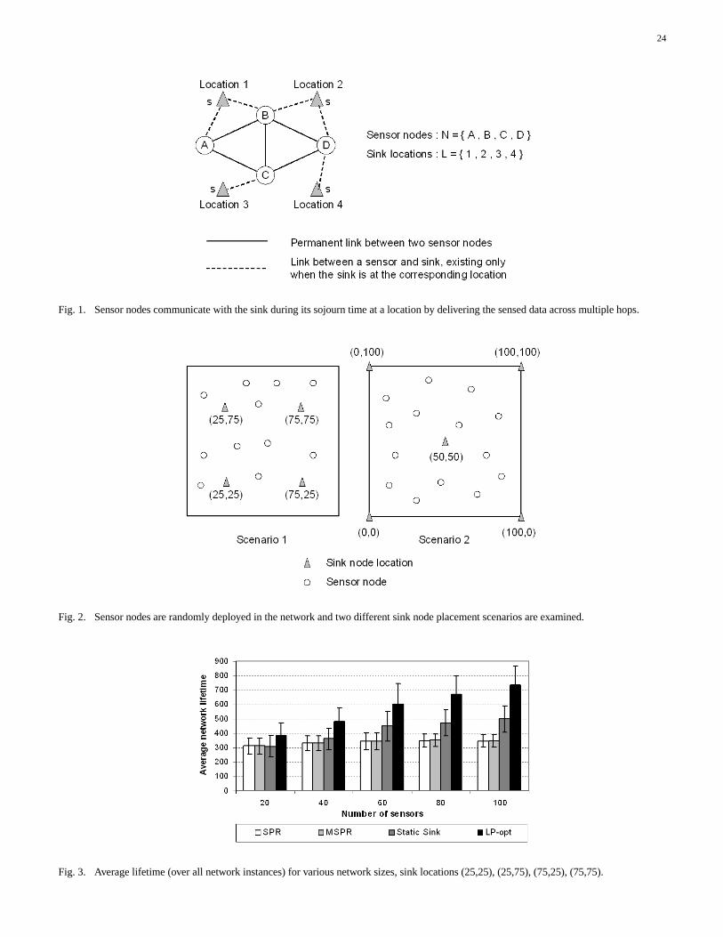
Consider for example the wireless sensor network shown in Fig. 1. Sensor nodes B and C are in the

transmission range of A, regardless where the sink node is located. When s is placed at location 1, sensor

A can also communicate with s. Therefore, the set of neighboring nodes of sensor A for location 1 is

S1A = {B,C, s}. However, when s moves to locations 2, 3, 4, it is not in the transmission range of sensor

A. Hence, S2A = S3A = S4A = {B,C}. Similarly for another sensor node, say node C, we have that

S1C = S2C = S4C = {A,B,D}, while S3C = {A,B,D, s}.

Every sensor i ∈ N has an initial amount of battery energy Ei > 0. The sink node has no energy

constraint, since it is typically a special node (different than the sensors) with plenty of battery energy which

can also be easily renewed. The transmission energy consumed at sensor i to transmit a data unit to its

neighboring node j is denoted by eTij > 0 and the energy consumed for reception by the receiver j is denoted

by eRij > 0. Note that the energy expenditure for an information unit transmitted by sensor i depends

on the next hop node and is not necessarily the same for every neighboring node j. These quantities are

network parameters determined by the energy dissipation model used. They usually depend on the physical

distance between the nodes and other environmental and technological factors which are not addressed here

1Another approach is to assume that there are two mobile sinks, such that one of them is at the current location and the other one is placed atthe location to be considered next. Hence, there is no additional time spent between two consecutive locations. Alternatively, if the sensor nodeshave enough buffer capacity, they can store their sensed data and wait until the sink node arrives at the new location.

8

in detail. In any case, we note that our formulation of the problem that follows does not depend on the energy

consumption model used.

The above description of the wireless sensor network indicates that in order to transfer the information

from the sensors to the sink, two complementary algorithms are necessary:

• a scheduling algorithm that determines for every location l ∈ L the duration tl for which the sink node

stays at that place,

• a routing algorithm to find the appropriate energy-efficient paths from every sensor node to the sink, for

every location l ∈ L for which tl > 0.

Since the sink node can be found in different places during network operation, the decision of the routing

algorithm depends on the location of the sink. Let qlij be the rate at which information is transmitted from

sensor i to its neighboring node j, to be assigned by the routing algorithm during time tl. For each qlij ,

there is a constraint qlij ≤ qmaxij , where qmaxij is the maximum possible rate at which information can be

transmitted from i to j. These bounds can be viewed as link capacity constraints determined by the network

environment. In addition to these link constraints, there is a power constraint for every sensor node. That

is, for every sink location l ∈ L, the power expenditure at sensor i ∈ N incurred by the transmissions and

receptions of i during time tl cannot exceed a maximum value Pi. This value can reflect the limitations

imposed by the hardware of the sensors (transceiver circuitry, power unit, etc.).

The overall objective is to maximize the duration of network operation before a sensor node drains out of

battery energy for the first time. In our model, the network lifetime is equal to the sum of the sojourn times

of the sink at all possible locations (see Section III-B below). The sojourn times are constrained by the fact

that the total energy consumed by each sensor node when the sink stays at different locations cannot exceed

the sensor’s initial amount of energy. Furthermore, the constraints on transmission rates and the power of

sensors are also taken into consideration. We summarize in Table I the notation most commonly used in this

paper for reader convenience. The last quantity in the table is introduced in the following section.

Note 1: The above description implies that we look at the system from the network layer perspective, i.e.,

9

the effect of the MAC layer and the related interference is not addressed here directly. This can be considered

as a valid working assumption, an approach followed by many previous works in order to reduce the problem

formulation complexity. However, we note that some of the implications imposed by layers lower than the

network layer can be incorporated into our model. For example, in a high interference environment the

energy expenditures eTij , eRij in general will become “worse” (increase) in order to reflect the fact that more

energy is required for communication. The signal-to-interference ratio requirements in a congested network

can also be incorporated into the link constraints qmaxij , since a smaller value at this bound will prevent sensor

i from sending many packets to j.

B. Linear Programming Formulation

In the following we show that our optimization problem can be written as a Linear Programming (LP)

problem [24]. We disregard any specific details of battery technology and assume that the power and,

consequently, energy expenditures are directly proportional to the rate at which information is transmit-

ted/received. Given the sink sojourn times tl and the information transfer rates qlij , i ∈ N , j ∈ Sli , l ∈ L, the

power (energy per time unit) consumed at sensor node i when the sink is placed at location l is given by

Xj∈Sli

eTijqlij +

Xj:i∈Slj

eRjiqlji, (1)

while the corresponding energy consumption for time duration tl is given by

⎛⎝Xj∈Sli

eTijqlij +

Xj:i∈Slj

eRjiqlji

⎞⎠ tl. (2)

The total energy consumed at sensor i during network operation is the sum of the quantities in (2) over all

locations l ∈ L, that is, Xl∈L

Xj∈Sli

eTijqlijtl +

Xl∈L

Xj:i∈Slj

eRjiqljitl. (3)

10

The network lifetime defined as the length of time until the first battery drain-out among all sensor nodes in

N , can also be expressed as the sum of the sojourn times of the sink at all possible locations,

Xl∈L

tl. (4)

Our goal is to find the sink sojourn times tl and the information transfer rates qlij , i ∈ N , j ∈ Sli, l ∈ L,

that maximize the lifetime of the network under the flow conservation condition and under the constraint that

the total energy consumed by each sensor node when the sink stays at different locations cannot exceed the

sensor’s initial amount of energy. Moreover, the constraints on transmission rates and the power expenditures

of sensors must also be taken into account. From the above definitions, the problem of maximizing the

overall network lifetime can be written as follows:

MaximizeXl∈L

tl subject to (5)

tl ≥ 0, l ∈ L, (6)

0 ≤ qlij ≤ qmaxij , i ∈ N, j ∈ Sli, l ∈ L, (7)

Xj∈Sli

eTijqlij +

Xj:i∈Slj

eRjiqlji ≤ Pi, i ∈ N, l ∈ L, (8)

Xl∈L

Xj∈Sli

eTijqlijtl +

Xl∈L

Xj:i∈Slj

eRjiqljitl ≤ Ei, i ∈ N, (9)

Xj:i∈Slj

qlji +Qi =Xj∈Sli

qlij, i ∈ N, l ∈ L. (10)

Note that the flow conservation condition (10) applies to each location l ∈ L separately. That is, for every

location of the sink, the total incoming information transfer rate plus the information generation rate at a

sensor node equals the total outgoing information transfer rate from the sensor. Since the sink node s is the

11

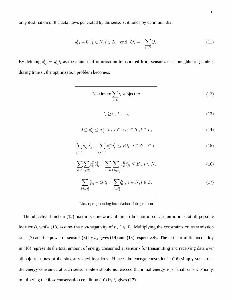
only destination of the data flows generated by the sensors, it holds by definition that

qlsj = 0, j ∈ N, l ∈ L, and Qs = −Xi∈N

Qi. (11)

By defining bqlij = qlijtl as the amount of information transmitted from sensor i to its neighboring node j

during time tl, the optimization problem becomes:

MaximizeXl∈L

tl subject to (12)

tl ≥ 0, l ∈ L, (13)

0 ≤ bqlij ≤ qmaxij tl, i ∈ N, j ∈ Sli, l ∈ L, (14)

Xj∈Sli

eTijbqlij + Xj:i∈Slj

eRjibqlji ≤ Pitl, i ∈ N, l ∈ L, (15)

Xl∈L

Xj∈Sli

eTijbqlij +Xl∈L

Xj:i∈Slj

eRjibqlji ≤ Ei, i ∈ N, (16)

Xj:i∈Slj

bqlji +Qitl =Xj∈Sli

bqlij, i ∈ N, l ∈ L. (17)

Linear programming formulation of the problem

The objective function (12) maximizes network lifetime (the sum of sink sojourn times at all possible

locations), while (13) assures the non-negativity of tl, l ∈ L. Multiplying the constraints on transmission

rates (7) and the power of sensors (8) by tl, gives (14) and (15) respectively. The left part of the inequality

in (16) represents the total amount of energy consumed at sensor i for transmitting and receiving data over

all sojourn times of the sink at visited locations. Hence, the energy constraint in (16) simply states that

the energy consumed at each sensor node i should not exceed the initial energy Ei of that sensor. Finally,

multiplying the flow conservation condition (10) by tl gives (17).

12

The linear programming model above determines for every location l ∈ L the duration tl for which the

sink node stays at that place and the quantities bqlij , i ∈ N , j ∈ Sli, so that the network lifetime is maximized.

The information transfer rates can also be computed as qlij = bqlij/tl and, therefore, the model provides an

optimal solution to both problems described earlier, the scheduling and the routing problem. If the optimal

value for a tl is 0, the sink does not visit location l. Every location l ∈ L for which the optimal tl is positive,

is visited by the sink for a time duration equal to tl. The sink visiting order is not important since the

traveling time of the sink between two locations is considered negligible and the information generation rate

is independent of time.

A more general version of our linear programming formulation is to consider that while the sink node

is at location l ∈ L, the information transfer rates qlij , i ∈ N , j ∈ Sli , can change. It may seem plausible

that by modifying the rate qlij at which information is transmitted from sensor i to its neighboring node j

during time tl, the amounts of remaining battery energy of the sensors can be utilized more efficiently and,

therefore, the duration of network operation can be prolonged. However, it is shown in the Appendix that

this generalization of the problem does not result in an improvement for the lifetime of the network.

Note 2: The fact that the energy expenditures eTij , eRij and the rates qlij , are not restricted to a finite discrete

set of values, implies an ideal power control sensor network. That is, each sensor is assumed to be able

to adjust its transmission power accordingly, depending on the next hop node. This assumption is usually

considered as an advantage by many researchers, since it prevents a sensor from spending more power for

transmission than the power that it actually needs. However, due to hardware constraints, in practice there

may be only little (a few power levels) power control in a real system. Taking this limitation into account

is beyond the scope of current work. The problem becomes a discrete optimization one, and cannot be

addressed directly by the proposed model. A trivial solution would be to solve the linear program and adjust

the transmission power of each sensor to the minimum value that is larger than the one given by the model.

However, a different approach is necessary in order to minimize the gap between theory and practice when

taking the limitation of a finite set of discrete power levels into account.

13

IV. NUMERICAL RESULTS

A. Description of the Compared Models

In this section we describe the models that we compare in order to evaluate numerically the performance

of our linear programming formulation. Inside the parenthesis we give the abbreviation that we use for each

model in the next section where we present the simulation results.

1) Linear Programming Model with Shortest Path Routing (SPR): This is a generalization of the ap-

proach followed in [23], so that it can be applied to general networks (the approach in [23] is restricted

only to square grid networks with homogeneous sensors and no power control). The LP model determines

only the sojourn times of the sink at every location l ∈ L and, therefore, it provides a solution only to the

scheduling problem described earlier. The routing problem is solved using a shortest path algorithm, where

the cost of a path depends on the number of hops and the transmission energy requirement of each hop (in

[23] there is no power control and the algorithm reduces to a minimum-number-of-hops routing algorithm).

The shortest path algorithm used to route the packets to the sink does not take into account the remaining

energy of the sensors, thus resulting in an overall network lifetime which is not optimal.

2) Linear Programming Model with Multiple Shortest Path Routing (MSPR): When there are multiple

shortest paths, the authors in [23] select two of them and alternate the route between these two paths. Moti-

vated by this variation, we modify the previous model so that the routing algorithm uses all existing shortest

paths from a sensor to the sink. The LP model which determines the sink sojourn times remains the same.

3) Linear Programming Model for the Static Sink case (Static Sink): When the sink remains static, we

determine the lifetime achieved at every location l ∈ L separately and select the one that gives the maximum

value. Given the location that maximizes lifetime, the sink stays there until a sensor node runs out of battery

energy for the first time and does not move to another place. For each location l ∈ L separately we use the

linear programming formulation given in Section III-B, replacing L by L0= {l}. Therefore, the Static Sink

model maximizes lifetime for every location, but it is not optimal for the overall objective which is the sum

of the sink sojourn times at all possible locations.

14

4) Optimal Linear Programming Formulation (LP-opt): This is the LP model proposed in Section III-B

which provides the optimal solution to the scheduling and the routing problem and gives the best achievable

overall network lifetime.

B. Performance Evaluation Through Simulations

In this section we compare numerically for various networks with different sizes and sink node placements

the performance of the four models previously described. The simulations that follow attempt to model the

following physical environment in a wireless sensor network. Assume that the sensor nodes are randomly

deployed on a terrain where there are various obstacles that may prohibit direct communication of certain

sensors. Assume also that the sink can be located in certain places inside the terrain (not necessarily co-

located with the sensor nodes) and that, for a given location, the sink is not within the transmission range of

every sensor. That is, multi-hop routing may be needed in order to transfer the information from a sensor to

the sink. We would like to evaluate the performance of the models in such an environment.

The figures that follow represent the averages of the results obtained from 100 randomly generated net-

work instances for each network size considered. We generate random networks with a specified number

of sensor nodes (20, 40, ..., 100) as follows. We fix a square grid of 100 × 100 points. A number of these

points is randomly selected with uniform probability to represent the sensor nodes of the network. Note that

the placement of the sensors does not form a grid network, but models a random deployment of the sensors

on the terrain. The transmission energy consumed at sensor i to transmit a data unit to its neighboring sen-

sor j depends on the distance d(i,j) between the two sensors and is given by eTij = d2(i,j). For simplicity in

performing the experiments, we assume that the energy consumed by the receiver j is small and thus can

be neglected. Note that this assumption is not restrictive (in any case, the reception cost is included in our

LP formulation) and does not affect intensely the relative performance of the compared models. For each

network instance there is a constraint on the maximum transmission energy expenditure among sensors,

eTmax, which is defined as the smallest value that guarantees connectivity among the sensor nodes. Hence, a

sensor node j is a neighbor of i if eTij ≤ eTmax. This constraint results in sparsely connected networks where

15

multi-hop routing is necessary among the sensor nodes.

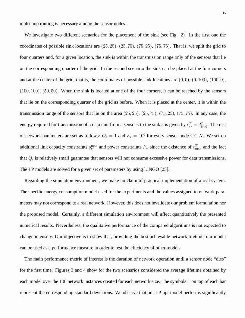
We investigate two different scenarios for the placement of the sink (see Fig. 2). In the first one the

coordinates of possible sink locations are (25, 25), (25, 75), (75, 25), (75, 75). That is, we split the grid to

four quarters and, for a given location, the sink is within the transmission range only of the sensors that lie

on the corresponding quarter of the grid. In the second scenario the sink can be placed at the four corners

and at the center of the grid, that is, the coordinates of possible sink locations are (0, 0), (0, 100), (100, 0),

(100, 100), (50, 50). When the sink is located at one of the four corners, it can be reached by the sensors

that lie on the corresponding quarter of the grid as before. When it is placed at the center, it is within the

transmission range of the sensors that lie on the area (25, 25), (25, 75), (75, 25), (75, 75). In any case, the

energy required for transmission of a data unit from a sensor i to the sink s is given by eTis = d2(i,s). The rest

of network parameters are set as follows: Qi = 1 and Ei = 106 for every sensor node i ∈ N . We set no

additional link capacity constraints qmaxij and power constraints Pi, since the existence of eTmax and the fact

that Qi is relatively small guarantee that sensors will not consume excessive power for data transmissions.

The LP models are solved for a given set of parameters by using LINGO [25].

Regarding the simulation environment, we make no claim of practical implementation of a real system.

The specific energy consumption model used for the experiments and the values assigned to network para-

meters may not correspond to a real network. However, this does not invalidate our problem formulation nor

the proposed model. Certainly, a different simulation environment will affect quantitatively the presented

numerical results. Nevertheless, the qualitative performance of the compared algorithms is not expected to

change intensely. Our objective is to show that, providing the best achievable network lifetime, our model

can be used as a performance measure in order to test the efficiency of other models.

The main performance metric of interest is the duration of network operation until a sensor node “dies”

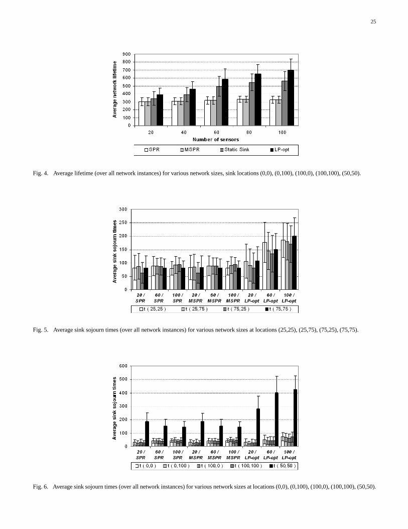
for the first time. Figures 3 and 4 show for the two scenarios considered the average lifetime obtained by

each model over the 100 network instances created for each network size. The symbols >⊥ on top of each bar

represent the corresponding standard deviations. We observe that our LP-opt model performs significantly

16

better than the other three models for all networks examined. The lifetime achieved by LP-opt in Fig. 3

is 23.5% higher than that of SPR and 23.8% higher than that of Static Sink for |N | = 20, while these

percentages rise to 111.9% and 47.2%, respectively, for |N | = 100. In Fig. 4 the lifetime achieved by

LP-opt is 28.8% higher than that of SPR and 14% higher than that of Static Sink for |N | = 20, while the

corresponding percentages for |N | = 100 are 114.4% and 24.5%. We see that in both figures the lifetime

improvement ratio increases with the network size. As the network size increases, the density of sensor

nodes (number of sensors per unit area) increases as well. Hence, there are more alternative paths which

can be used by the LP-opt model to route the information from every sensor to the sink. This results in

a more balanced energy depletion among the sensor nodes and, therefore, the lifetime achieved by LP-opt

is considerably higher than the other three models. Note that the energy consumption model is the same

for all network sizes and does not incorporate any additional energy costs for increased interference in

larger networks or energy spent in idle state, etc. Hence, larger networks appear to perform better in our

simulations, which cannot be taken for granted in practice. However, it still remains the fact that the larger

interference induced by increasing the network size, can be mitigated in part by the availability of more

alternative paths provided by our model.

An interesting observation is that SPR and MSPR perform almost the same for all networks examined.

This is due to the fact that the sensor nodes are randomly deployed inside the network and the transmission

energy requirements depend on the distance between the communicating nodes. Hence, the costs of multiple

paths that may exist from a sensor node to the sink are typically different and, most of the times, there exists

only one shortest path to route the packets. A notable difference in the performance of these two models

would appear in some special cases (e.g., grid networks). However, our aim is to evaluate the performance of

the models in networks where the sensor nodes are realistically randomly placed in the sensor field. Another

interesting observation is that Static Sink performs better than both SPR and MSPR. This is because the

Static Sink model uses the optimal linear programming formulation of Section III-B and maximizes the

lifetime for every location separately. Although the overall network lifetime achieved is shorter than LP-opt,

17

since the sensor nodes close to the sink always relay the packets of all other sensors which drains them of

their energy quite faster, it is still higher than that of SPR and MSPR which leave the routing problem outside

the linear programming formulation (using a shortest path algorithm which is not optimal).

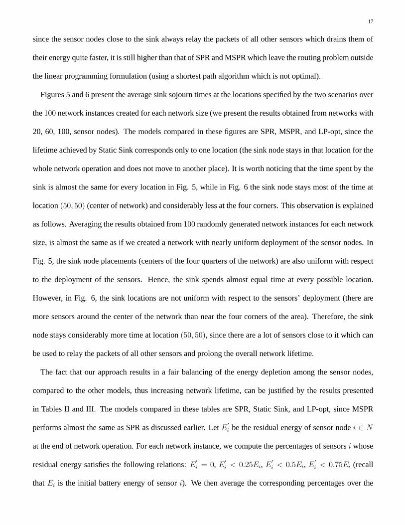
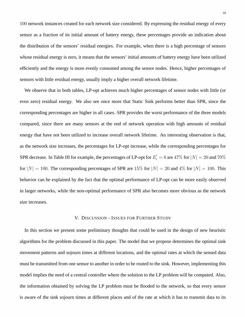
Figures 5 and 6 present the average sink sojourn times at the locations specified by the two scenarios over

the 100 network instances created for each network size (we present the results obtained from networks with

20, 60, 100, sensor nodes). The models compared in these figures are SPR, MSPR, and LP-opt, since the

lifetime achieved by Static Sink corresponds only to one location (the sink node stays in that location for the

whole network operation and does not move to another place). It is worth noticing that the time spent by the

sink is almost the same for every location in Fig. 5, while in Fig. 6 the sink node stays most of the time at

location (50, 50) (center of network) and considerably less at the four corners. This observation is explained

as follows. Averaging the results obtained from 100 randomly generated network instances for each network

size, is almost the same as if we created a network with nearly uniform deployment of the sensor nodes. In

Fig. 5, the sink node placements (centers of the four quarters of the network) are also uniform with respect

to the deployment of the sensors. Hence, the sink spends almost equal time at every possible location.

However, in Fig. 6, the sink locations are not uniform with respect to the sensors’ deployment (there are

more sensors around the center of the network than near the four corners of the area). Therefore, the sink

node stays considerably more time at location (50, 50), since there are a lot of sensors close to it which can

be used to relay the packets of all other sensors and prolong the overall network lifetime.

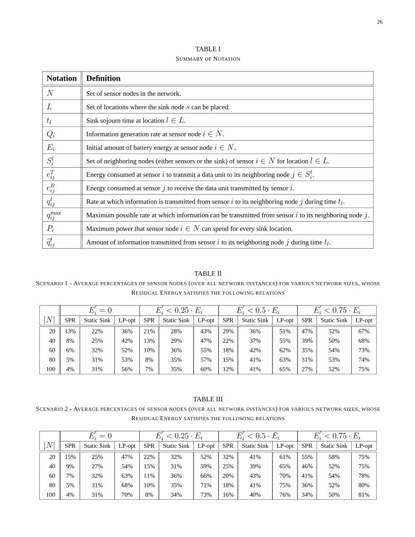
The fact that our approach results in a fair balancing of the energy depletion among the sensor nodes,

compared to the other models, thus increasing network lifetime, can be justified by the results presented

in Tables II and III. The models compared in these tables are SPR, Static Sink, and LP-opt, since MSPR

performs almost the same as SPR as discussed earlier. Let E0i be the residual energy of sensor node i ∈ N

at the end of network operation. For each network instance, we compute the percentages of sensors i whose

residual energy satisfies the following relations: E0i = 0, E0

i < 0.25Ei, E0i < 0.5Ei, E

0i < 0.75Ei (recall

that Ei is the initial battery energy of sensor i). We then average the corresponding percentages over the

18

100 network instances created for each network size considered. By expressing the residual energy of every

sensor as a fraction of its initial amount of battery energy, these percentages provide an indication about

the distribution of the sensors’ residual energies. For example, when there is a high percentage of sensors

whose residual energy is zero, it means that the sensors’ initial amounts of battery energy have been utilized

efficiently and the energy is more evenly consumed among the sensor nodes. Hence, higher percentages of

sensors with little residual energy, usually imply a higher overall network lifetime.

We observe that in both tables, LP-opt achieves much higher percentages of sensor nodes with little (or

even zero) residual energy. We also see once more that Static Sink performs better than SPR, since the

corresponding percentages are higher in all cases. SPR provides the worst performance of the three models

compared, since there are many sensors at the end of network operation with high amounts of residual

energy that have not been utilized to increase overall network lifetime. An interesting observation is that,

as the network size increases, the percentages for LP-opt increase, while the corresponding percentages for

SPR decrease. In Table III for example, the percentages of LP-opt for E0i = 0 are 47% for |N | = 20 and 70%

for |N | = 100. The corresponding percentages of SPR are 15% for |N | = 20 and 4% for |N | = 100. This

behavior can be explained by the fact that the optimal performance of LP-opt can be more easily observed

in larger networks, while the non-optimal performance of SPR also becomes more obvious as the network

size increases.

V. DISCUSSION - ISSUES FOR FURTHER STUDY

In this section we present some preliminary thoughts that could be used in the design of new heuristic

algorithms for the problem discussed in this paper. The model that we propose determines the optimal sink

movement patterns and sojourn times at different locations, and the optimal rates at which the sensed data

must be transmitted from one sensor to another in order to be routed to the sink. However, implementing this

model implies the need of a central controller where the solution to the LP problem will be computed. Also,

the information obtained by solving the LP problem must be flooded to the network, so that every sensor

is aware of the sink sojourn times at different places and of the rate at which it has to transmit data to its

19

neighboring nodes. We note that the suboptimal algorithms proposed in previous work, described in Section

IV-A, are also centralized. In our setup, we assume constant information generation rates (not necessarily

the same for all sensors), while the previous approaches assume the same constant information generation

rate for every sensor node.

An interesting issue for further study is the implementation of our model in a distributed environment

where the sink sojourn times and the information transfer rates are not determined by a central node (possibly

the sink). Distributed maximum lifetime routing algorithms for the case of fixed sink node location exist in

the literature [26], but cannot be easily generalized to address the mobile sink problem.

Another interesting issue for future research is to develop an on-line algorithm which can be used in an

adaptive environment, where the sensor nodes do not know the schedule of the sink in advance and the

information generation process is arbitrary for every sensor. Such an algorithm could be as follows. We

can use one of the energy-aware routing algorithms referenced in Section II for a given location of the sink.

After an update interval, the sink node decides whether to stay at its current location or move to another

place. The remaining lifetimes of the sensors can be used by the routing algorithm to determine new paths

to the sink, so that the bottleneck nodes are avoided and a more balanced energy depletion among the sensor

nodes is achieved. Such an algorithm would be greedy in a sense that the sink does not decide its schedule

in advance, but moves from one location to another determining on-line the time to spend in every location

according to the remaining lifetimes of the sensors. While this approach seems plausible, many issues have

to be addressed for a complete description. Moreover, a careful evaluation must be performed in order to

make sure that the overall approach works. We note that the optimal algorithm proposed in this work can

be used as a yardstick against which one can compare the performance of new algorithms that might be

proposed in the future to address the above-mentioned problems.

Other directions for further study include taking into account a limitation in power control, i.e., consid-

ering only a few discrete power levels for the sensors. This limitation converts the problem to a discrete

optimization one and a different approach is necessary to address the new issues that arise. Finally, addi-

20

tional simulations could be performed in order to consider different energy consumption models that take

into account energy costs incurred by increased interference, MAC layer issues, idle state of the sensors, etc.

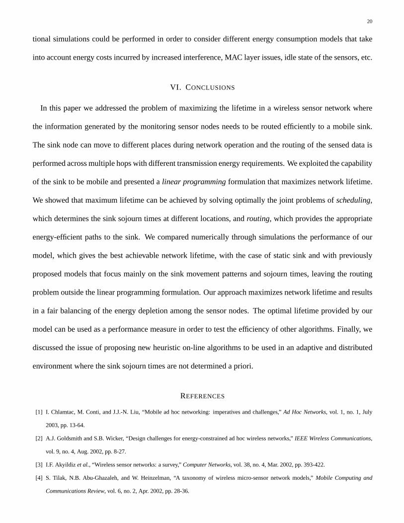
VI. CONCLUSIONS

In this paper we addressed the problem of maximizing the lifetime in a wireless sensor network where

the information generated by the monitoring sensor nodes needs to be routed efficiently to a mobile sink.

The sink node can move to different places during network operation and the routing of the sensed data is

performed across multiple hops with different transmission energy requirements. We exploited the capability

of the sink to be mobile and presented a linear programming formulation that maximizes network lifetime.

We showed that maximum lifetime can be achieved by solving optimally the joint problems of scheduling,

which determines the sink sojourn times at different locations, and routing, which provides the appropriate

energy-efficient paths to the sink. We compared numerically through simulations the performance of our

model, which gives the best achievable network lifetime, with the case of static sink and with previously

proposed models that focus mainly on the sink movement patterns and sojourn times, leaving the routing

problem outside the linear programming formulation. Our approach maximizes network lifetime and results

in a fair balancing of the energy depletion among the sensor nodes. The optimal lifetime provided by our

model can be used as a performance measure in order to test the efficiency of other algorithms. Finally, we

discussed the issue of proposing new heuristic on-line algorithms to be used in an adaptive and distributed

environment where the sink sojourn times are not determined a priori.

REFERENCES

[1] I. Chlamtac, M. Conti, and J.J.-N. Liu, “Mobile ad hoc networking: imperatives and challenges,” Ad Hoc Networks, vol. 1, no. 1, July

2003, pp. 13-64.

[2] A.J. Goldsmith and S.B. Wicker, “Design challenges for energy-constrained ad hoc wireless networks,” IEEE Wireless Communications,

vol. 9, no. 4, Aug. 2002, pp. 8-27.

[3] I.F. Akyildiz et al., “Wireless sensor networks: a survey,” Computer Networks, vol. 38, no. 4, Mar. 2002, pp. 393-422.

[4] S. Tilak, N.B. Abu-Ghazaleh, and W. Heinzelman, “A taxonomy of wireless micro-sensor network models,” Mobile Computing and

Communications Review, vol. 6, no. 2, Apr. 2002, pp. 28-36.

21

[5] I.F. Akyildiz and I.H. Kasimoglu, “Wireless sensor and actor networks: research challenges,” Ad Hoc Networks, vol. 2, no. 4, Oct. 2004,

pp. 351-367.

[6] J.-H. Chang and L. Tassiulas, “Routing for maximum system lifetime in wireless ad-hoc networks,” in Proc. of 37th Annual Allerton Conf.

on Communication, Control, and Computing, Monticello, IL, Sept.1999.

[7] J.-H. Chang and L. Tassiulas, “Energy conserving routing in wireless ad-hoc networks,” in Proc. of IEEE INFOCOM, Tel-Aviv, Israel,

Mar. 2000, pp. 22-31.

[8] J.-H. Chang and L. Tassiulas, “Maximum lifetime routing in wireless sensor networks,” in Proc. of ATIRP, College Park, MD, Mar. 2000.

[9] J.-H. Chang and L. Tassiulas, “Maximum lifetime routing in wireless sensor networks,” IEEE/ACM Trans. on Networking, vol. 12, no. 4,

Aug. 2004, pp. 609-619.

[10] K. Kalpakis, K. Dasgupta, and P. Namjoshi, “Efficient algorithms for maximum lifetime data gathering and aggregation in wireless sensor

networks,” Computer Networks, vol. 42, no. 6, Aug. 2003, pp. 697-716.

[11] Y.T. Hou, Y. Shi, and H.D. Sherali, “Rate allocation in wireless sensor networks with network lifetime requirement,” in Proc. of ACM

MobiHoc, Roppongi, Japan, May 2004, pp. 67-77.

[12] H.-W. Yoon et al., “Energy efficient routing with power management to increase network lifetime in sensor networks,” in Proc. of ICCSA,

Assisi, Italy, May 2004, LNCS 3046, pp. 46-55.

[13] K. Akkaya and M. Younis, “Energy-aware delay-constrained routing in wireless sensor networks,” Int. J. of Communication Systems, vol.

17, no. 6, Aug. 2004, pp. 663-687.

[14] L. Zhang et al., “A fair energy conserving routing algorithm for wireless sensor networks,” in Proc. of EUSAI, Eindhoven, The Netherlands,

Nov. 2004, LNCS 3295, pp. 303-314.

[15] A. Bogdanov, E. Maneva, and S. Riesenfeld, “Power-aware base station positioning for sensor networks,” in Proc. of IEEE INFOCOM,

Hong Kong, Mar. 2004.

[16] E.I. Oyman and C. Ersoy, “Multiple sink network design problem in large scale wireless sensor networks,” in Proc. of ICC, Paris, France,

June 2004.

[17] A. Chakrabarti, A. Sabharwal, and B. Aazhang, “Using predictable observer mobility for power efficient design of sensor networks,” in

Proc. of IPSN, Palo Alto, CA, Apr. 2003, LNCS 2634, pp. 129-145.

[18] H.S. Kim, T.F. Abdelzaher, and W.H. Kwon, “Minimum-energy asynchronous dissemination to mobile sinks in wireless sensor networks,”

in Proc. of ACM SenSys, Los Angeles, CA, Nov. 2003, pp. 193-204.

[19] S.R. Gandham et al., “Energy efficient schemes for wireless sensor networks with multiple mobile base stations,” in Proc. of IEEE

GLOBECOM, San Francisco, CA, Dec. 2003, pp. 377-381.

[20] R. Urgaonkar and B. Krishnamachari, “FLOW: An efficient forwarding scheme to mobile sink in wireless sensor networks,” in Poster of

IEEE SECON, Santa Clara, CA, Oct. 2004.

[21] P. Baruah, R. Urgaonkar, and B. Krishnamachari, “Learning-enforced time domain routing to mobile sinks in wireless sensor fields,” in

Proc. of IEEE EmNetS-I, Tampa, FL, Nov. 2004.

[22] Y. Tirta et al., “Efficient collection of sensor data in remote fields using mobile collectors,” in Proc. of ICCCN, Chicago, IL, Oct. 2004.

[23] Z.M. Wang et al., “Exploiting sink mobility for maximizing sensor networks lifetime,” in Proc. of HICSS, Big Island, Hawaii, Jan. 2005.

22

[24] S.G. Nash and A. Sofer, Linear and Nonlinear Programming, New York: McGraw-Hill, 1996.

[25] Lindo Systems Inc., http://www.lindo.com .

[26] R. Madan and S. Lall, “Distributed algorithms for maximum lifetime routing in wireless sensor networks,” in Proc. of IEEE GLOBECOM,

Dallas, TX, Nov.-Dec. 2004.

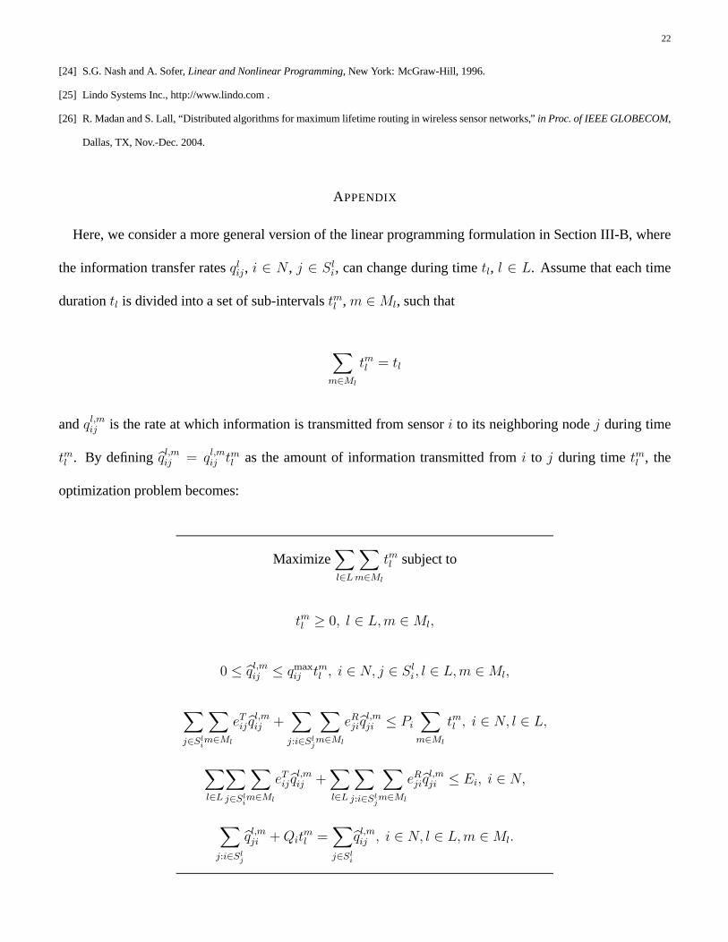
APPENDIX

Here, we consider a more general version of the linear programming formulation in Section III-B, where

the information transfer rates qlij , i ∈ N , j ∈ Sli , can change during time tl, l ∈ L. Assume that each time

duration tl is divided into a set of sub-intervals tml , m ∈Ml, such that

Xm∈Ml

tml = tl

and ql,mij is the rate at which information is transmitted from sensor i to its neighboring node j during time

tml . By defining bql,mij = ql,mij tml as the amount of information transmitted from i to j during time tml , the

optimization problem becomes:

MaximizeXl∈L

Xm∈Ml

tml subject to

tml ≥ 0, l ∈ L,m ∈Ml,

0 ≤ bql,mij ≤ qmaxij tml , i ∈ N, j ∈ Sli, l ∈ L,m ∈Ml,

Xj∈Sli

Xm∈Ml

eTijbql,mij +Xj:i∈Slj

Xm∈Ml

eRjibql,mji ≤ Pi

Xm∈Ml

tml , i ∈ N, l ∈ L,

Xl∈L

Xj∈Sli

Xm∈Ml

eTijbql,mij +Xl∈L

Xj:i∈Slj

Xm∈Ml

eRjibql,mji ≤ Ei, i ∈ N,

Xj:i∈Slj

bql,mji +Qitml =

Xj∈Sli

bql,mij , i ∈ N, l ∈ L,m ∈Ml.

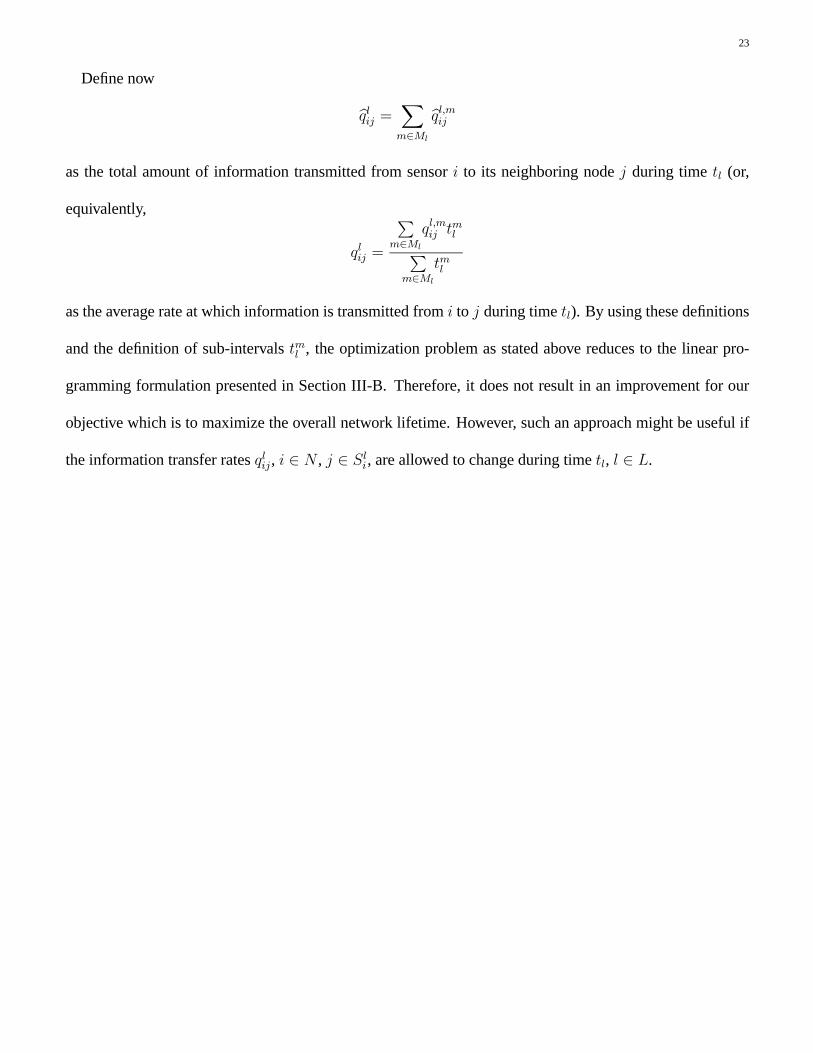
23

Define now

bqlij = Xm∈Ml

bql,mijas the total amount of information transmitted from sensor i to its neighboring node j during time tl (or,

equivalently,

qlij =

Pm∈Ml

ql,mij tmlPm∈Ml

tml

as the average rate at which information is transmitted from i to j during time tl). By using these definitions

and the definition of sub-intervals tml , the optimization problem as stated above reduces to the linear pro-

gramming formulation presented in Section III-B. Therefore, it does not result in an improvement for our

objective which is to maximize the overall network lifetime. However, such an approach might be useful if

the information transfer rates qlij , i ∈ N , j ∈ Sli, are allowed to change during time tl, l ∈ L.

24

Fig. 1. Sensor nodes communicate with the sink during its sojourn time at a location by delivering the sensed data across multiple hops.

Fig. 2. Sensor nodes are randomly deployed in the network and two different sink node placement scenarios are examined.

Fig. 3. Average lifetime (over all network instances) for various network sizes, sink locations (25,25), (25,75), (75,25), (75,75).

25

Fig. 4. Average lifetime (over all network instances) for various network sizes, sink locations (0,0), (0,100), (100,0), (100,100), (50,50).

Fig. 5. Average sink sojourn times (over all network instances) for various network sizes at locations (25,25), (25,75), (75,25), (75,75).

Fig. 6. Average sink sojourn times (over all network instances) for various network sizes at locations (0,0), (0,100), (100,0), (100,100), (50,50).

26

TABLE ISUMMARY OF NOTATION

Notation Definition

N Set of sensor nodes in the network.

L Set of locations where the sink node s can be placed.

tl Sink sojourn time at location l ∈ L.

Qi Information generation rate at sensor node i ∈ N .

Ei Initial amount of battery energy at sensor node i ∈ N .

Sli Set of neighboring nodes (either sensors or the sink) of sensor i ∈ N for location l ∈ L.

eTij Energy consumed at sensor i to transmit a data unit to its neighboring node j ∈ Sli .

eRij Energy consumed at sensor j to receive the data unit transmitted by sensor i.

qlij Rate at which information is transmitted from sensor i to its neighboring node j during time tl.

qmaxij Maximum possible rate at which information can be transmitted from sensor i to its neighboring node j.

Pi Maximum power that sensor node i ∈ N can spend for every sink location.bqlij Amount of information transmitted from sensor i to its neighboring node j during time tl.

TABLE IISCENARIO 1 - AVERAGE PERCENTAGES OF SENSOR NODES (OVER ALL NETWORK INSTANCES) FOR VARIOUS NETWORK SIZES, WHOSE

RESIDUAL ENERGY SATISFIES THE FOLLOWING RELATIONS

E0i = 0 E

0i < 0.25 ·Ei E

0i < 0.5 ·Ei E

0i < 0.75 · Ei

|N | SPR Static Sink LP-opt SPR Static Sink LP-opt SPR Static Sink LP-opt SPR Static Sink LP-opt

20 13% 22% 36% 21% 28% 43% 29% 36% 51% 47% 52% 67%40 8% 25% 42% 13% 29% 47% 22% 37% 55% 39% 50% 68%60 6% 32% 52% 10% 36% 55% 18% 42% 62% 35% 54% 73%80 5% 31% 53% 8% 35% 57% 15% 41% 63% 31% 53% 74%

100 4% 31% 56% 7% 35% 60% 12% 41% 65% 27% 52% 75%

TABLE IIISCENARIO 2 - AVERAGE PERCENTAGES OF SENSOR NODES (OVER ALL NETWORK INSTANCES) FOR VARIOUS NETWORK SIZES, WHOSE

RESIDUAL ENERGY SATISFIES THE FOLLOWING RELATIONS

E0i = 0 E

0i < 0.25 ·Ei E

0i < 0.5 ·Ei E

0i < 0.75 · Ei

|N | SPR Static Sink LP-opt SPR Static Sink LP-opt SPR Static Sink LP-opt SPR Static Sink LP-opt

20 15% 25% 47% 22% 32% 52% 32% 41% 61% 55% 58% 75%40 9% 27% 54% 15% 31% 59% 25% 39% 65% 46% 52% 75%60 7% 32% 63% 11% 36% 66% 20% 43% 70% 41% 54% 78%80 5% 31% 68% 10% 35% 71% 18% 41% 75% 36% 52% 80%

100 4% 31% 70% 8% 34% 73% 16% 40% 76% 34% 50% 81%