18it03 forney

IEEE TRANSACTIONS ON INFORMATION THEORY, VOL. IT-18, NO. 3, MAY 1972 363

[13] R. W. Lucky, J. Salz, and E. J. Weldon, Principles of Data Com- [15] E. R. Kretzmer, “General ization of a technique for binary data munication. New York: McGraw-Hill, 1968. communicat ion,” IEEE Trans. Commun. Technol. (Concise

[14] F. S. Hill& Jr., “The computat ion of error probability for digital Papers), vol. COM-14, pp. 67-68, Feb. 1966. transmission,” Bell Syst. Tech. J., vol. 50, pp. 2055-2077, July- [16] E. Hansler, “An upper bound of error probability in data trans- Aug. 1971. mission systems,” Nachrichtentech. Z., no. 12, pp. 625-627, 1970.

Maximum-Likelihood Seauence Estima tion of Digital Sequences i&he Presence of

Intersymbo l Interference G. DAVID FORNEY, JR., MEMBER, IEEE

Abstract-A maximum-likel ihood sequence estimator for a digital pulse-ampli tude-modulated sequence in the presence of finite intersymbol interference and white Gaussian noise is developed. The structure cbm- prises a sampled linear filter, called a whitened matched filter, and a recursive nonl inear processor, called the Viterbi algorithm. The outputs of the whitened matched filter, sampled once for each input symbol, are shown to form a set of suillcient statistics for estimation of the input sequence, a fact that makes obvious some earlier results on opt imum linear processors. The Viterbi algorithm is easier to implement than earlier opt imum nonl inear processors and its per formance can be straightforwardly and accurately estimated. It is shown that per formance (by whatever criterion) is effectively as good as could be attained by any receiver structure and in many cases is as good as if intersymbol interference were absent. Finally, a simplified but effectively opt imum algorithm suitable for the most popular part ial-response schemes is described.

INTRODUCTION

I NTERSYMBOL interference arises in pulse-modulation systems whenever the effects of one transmitted pulse

are not al lowed to die away completely before the trans- m ission of the next. It is the primary impediment to reliable high-rate digital transmission over high signal-to-noise ratio narrow-bandwidth channels such as voice-grade telephone circuits. Intersymbol interference is also introduced deliberately for the purpose of spectral shaping in certain modu lation schemes for narrow-band channels, called duobinary, partial-response, and the like [ l]-[3].

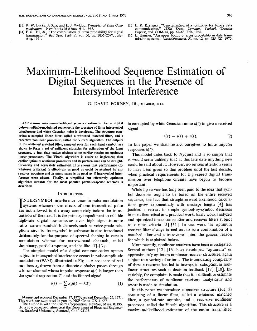
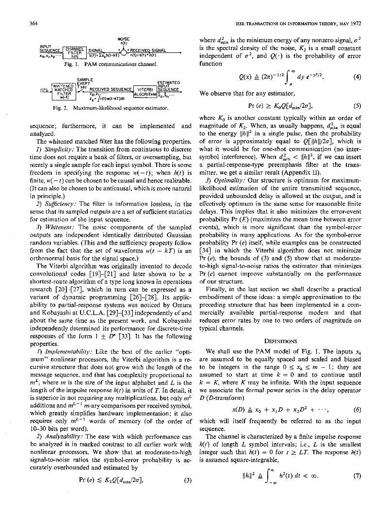
The simplest mode l of a digital communicat ion system subject to intersymbol interference occurs in pulse amp litude modu lation (PAM), illustrated in F ig. 1. A sequence of real numbers x, drawn from a discrete alphabet passes through a linear channel whose impulse response h(t) is longer than the symbol separation T, and the filtered signal

s(t) = c x,h(t - kT) k

(1)

Manuscript received December 17,197O; revised December 29, 1971. This work was supported in part by NSF Grant GK-31627.

The author is with the Codex Corporation, Newton, Mass. 02195. He is now on leave of absence at the Department of Electrical Engineer- ing, Stanford University, Stanford, Calif. 94305.

is corrupted by white Gaussian noise n(t) to give a received signal

r(t) = s(t) + n(t). (2)

In this paper we shall restrict ourselves to finite impulse responses h(t).

This mode l dates back to Nyquist and is so simple that it would seem unlikely that at this late date anything new could be said about it. However, no serious attention seems to have been given to this problem until the last decade, when practical requirements for h igh-speed digital trans- m ission over telephone circuits have begun to become important.

Wh ile lip service has long been paid to the idea that symbol decisions ought to be based on the entire received sequence, the fact that straightforward likelihood calcula- tions grow exponentially with message length [4] has justified a retreat to simple symbol-by-symbol decisions in most theoretical and practical work. Early work analyzed and optimized linear transmitter and receiver filters subject to various criteria [5]-[l l]. In this work the opt imum receiver filter always turned out to be a combination of a matched filter and a transversal filter, the general reason for which is explained below.

More recently, nonlinear receivers have been investigated. Several authors [12]-[16] have developed “opt imum” or approximately opt imum nonlinear receiver structures, again subject to a variety of criteria. The intimidating complexity of these structures has led to interest in subopt imum nonlinear structures such as decision feedback [17], [18]. In- variably, the complaint is made that it is difficult to estimate the performance of nonlinear receivers analytically and resort is made to simulation.

In this paper we introduce a receiver structure (Fig. 2) consisting of a linear filter, called a whitened matched filter, a symbol-rate sampler, and a recursive nonlinear processor, called the Viterbi algorithm. This structure is a maximum-likel ihood estimator of the entire transmitted

364 IEEE TRANSACTIONS ON INFORMATION THEORY, MAY 1972

NOISE n(t)

where d,$,, is the minimum energy of any nonzero signal, 0’ SNEENCE r cF”gg- SlGtiAL- + + RECEIVED SIGNAL is the spectral density of the noise, Kz is a small constant . %%X2”’ h,t, s(t)= Zxkh(t-kT) ” r(t)=s(t)+n(t) independent of 02, and Q( *) is the probability of error

Fig. 1. PAM communications channel. function

s co

Q(x) A (2n)-“’ dy e-y2J2. (4) x

We observe that for any estimator,

Fig. 2. Maximum-likelihood sequence estimator. (5)

sequence; furthermore, it can be implemented and analyzed.

The whitened matched filter has the following properties. I) Simplicity: The transition from continuous to discrete

time does not require a bank of filters, or oversampling, but merely a single sample for each input symbol. There is some freedom in specifying the response w( - t); when h(t) is finite, w( - t) can be chosen to be causal and hence realizable. (It can also be chosen to be anticausal, which is more natural in principle.)

2) Suficiency : The filter is information lossless, in the sense that its sampled outputs are a set of sufficient statistics for estimation of the input sequence.

3) Whiteness: The noise components of the sampled outputs are independent identically distributed Gaussian random variables. (This and the sufficiency property follow from the fact that the set of waveforms w(t - kT) is an orthonormal basis for the signal space.)

The Viterbi algorithm was originally invented to decode convolutional codes [19]-[21] and later shown to be a shortest-route algorithm of a type long known in operations research [20]-[27], which in turn can be expressed as a variant of dynamic programming [26]-[28]. Its applic- ability to partial-response systems was noticed by Omura and Kobayashi at U.C.L.A. [29]-[33] independently of and about the same time as the present work, and Kobayashi independently determined its performance for discrete-time responses of the form 1 + D” [33]. It has the following properties.

1) Implementability: Like the best of the earlier “optimum” nonlinear processors, the Viterbi algorithm is a recursive structure that does not grow with the length of the message sequence, and that has complexity proportional to mL, where m is the size of the input alphabet and L is the length of the impulse response h(t) in units of T. In detail, it is superior in not requiring any multiplications, but only mL additions and mL-l m-ary comparisons per received symbol, which greatly simplifies hardware implementation; it also requires only mL- ’ words of memory (of the order of IO-30 bits per word).

2) Analyzability: The ease with which performance can be analyzed is in marked contrast to all earlier work with nonlinear processors. We show that at moderate-to-high signal-to-noise ratios the symbol-error probability is accurately overbounded and estimated by

Pr (4 5 JGQ[4,d2~1~ (3)

where K, is another constant typically within an order of magnitude of K2. When, as usually happens, d&, is equal to the energy llh11’ in a single pulse, then the probability of error is approximately equal to Q[ llhlj/2a], which is what it would be for one-shot communication (no intersymbol interference). When d,$,, < llhl12, if we can insert a partial-response-type preemphasis filter at the transmitter, we get a similar result (Appendix II).

3) Optimality: Our structure is optimum for maximum- likelihood estimation of the entire transmitted sequence, provided unbounded delay is allowed at the output, and is effectively optimum in the same sense for reasonable finite delays. This implies that it also minimizes the error-event probability Pr (E) (maximizes the mean time between error events), which is more significant than the symbol-error probability in many applications. As for the symbol-error probability Pr (e) itself, while examples can be constructed [34] in which the Viterbi algorithm does not minimize Pr (e), the bounds of (3) and (5) show that at moderate- to-high signal-to-noise ratios the estimator that minimizes Pr (e) cannot improve substantially on the performance of our structure.

Finally, in the last section we shall describe a practical embodiment of these ideas: a simple approximation to the preceding structure that has been implemented in a commercially available partial-response modem and that reduces error rates by one to two orders of magnitude on typical channels.

DEFINITIONS

We shall use the PAM model of Fig. 1. The inputs x, are assumed to be equally spaced and scaled and biased to be integers in the range 0 < x, < m - 1; they are assumed to start at time k = 0 and to continue until k = K, where K may be infinite. With the input sequence we associate the formal power series in the delay operator D (D-transform)

x(D) p x,, + x,D + x2D2 + . . . . G-3

which will itself frequently be referred to as the input sequence.

The channel is characterized by a finite impulse response h(t) of length L symbol intervals; i.e., L is the smallest integer such that h(t) = 0 for t 2 LT. The response h(t) is assumed square-integrable,

Ilhl12 4 ~- J h2(t) dt < 00.

-CB (7)

FORNEY: MAXIMUM-LIKELIHOOD SEQUENCE ESTIMATION 365

We define h’k)(t) A h(t - kT)

and use inner-product notation in which

s

00 [4tMt)l A a(t)b(t) dt.

-a,

and pulse autocorrelation function (8) &dD) = f (D)f CD- ‘P’,,(D). (19)

THE MATCHED FILTER

(9) The signal s(t) is defined as

Then the pulse autocorrelation coefficients of h(t) are s(t) & i x,h(t - kT) = f x,hck’(t). (20) k=O k=O

&-,. & [h’k’(t),h’k”(t)] The received signal r(t) is s(t) plus white Gaussian noise

i

s

n(t). m h(t - kT)h(t - k’T) dt, It is well known (see, for example, [35]) that in the

= -co detection of signals that are linear combinations of some Ik - k’J I L - 1 finite set of square-integrable basis functions hCk’(t), the

0, Ik - k’l 2 L. (10) outputs of a bank of matched filters, one matched to each

We define the pulse autocorrelation function of h(t) as basis function, form a set of sufficient statistics for estimat- ing the coefficients, Thus the K + I quantities

R(D) A i RkDk, (11) k=-v

where v = L - 1 is called the span of h(t). We shall also write R&D) when it is necessary to distinguish different autocorrelation functions.

The response h(t) may be regarded as a sequence of L chips h,(t), 0 < i I v, where h,(t) is a function that is nonzero only over the interval [O,T); i.e.,

h(t) = h,(t) + h,(t - T) + . . . + h&t - VT). (12)

Then it is natural to associate with h(t) the chip D-transform

W ,t) & i hi(t)D’, (13) i=O

which is a polynomial in D of degree v with coefficients in the set of functions over [O,r). It is easy to verify that the chip D-transform has the following properties.

1) The pulse autocorrelation function is given by

R(D) = [h(~,t),h(~-l,t)] = s

T

h(D,t)h(D-‘,t) dt. (14) 0

2) A transversal filter is a filter with response

g(t) = c gicyt - iT) (15)

for some set of coefficients gi. This response is not square integrable, but we assume the coefficients gi are square summable, xi gi2 < cc. We say a transversal filter g(t) is characterized by g(D) if

g(D) = c giDi. (16) I The chip D-transform g(D,t) of a transversal filter is

g(DJ) = g(D)@+ (17)

3) The cascade of a square-integrable filter with response g(r) and a transversal filter characterized by a square- summable j’(D) is a filter with square-integrable response h(t), chip D-transform

WA = .f(DldD,f> (181

ak Q [r(t>,h’k’(t>]

s m

= r(t)h(t - kT) dt, 0 I k I K (21) -03

form a set of sufficient statistics for estimation of the xk, 0 < k _< K, when K is finite. But these are simply the sampled outputs of a filter h(-t) matched to h(r). Hence we have the following proposition.

Proposition 1: When x(D) is finite, the sampled outputs uk [defined by (21)] of a filter matched to h(t) form a set of sufficient statistics for estimation of the input sequence x(D).

It is obvious on physical grounds that this property does not depend on x(D) being finite, but the corresponding result does not seem to be available in the literature. If x(D) is infinite the signals have infinite duration, so that the Karhunen-Loeve expansion is not applicable, and infinite energy, so that the generalization of Bharucha and Kadota [36] cannot be applied. We leave the proof to the reader, using his favorite definition of white Gaussian noise, which as usual is the only technical difficulty. (The Alexandrian method of dealing with this Gordian knot would be to de$& white Gaussian noise as any noise such that Prop- osition 1 is valid for infinite x(D) and any square integrable 40)

In view of the obviousness of Proposition 1, it is remark- able that it has not been much exploited previously in the intersymbol interference literature. (It does appear as a problem in Van Trees [37], attributed to Austin.) Some authors make the transition from continuous to discrete time by a sampler without a matched filter, with no explicit recognition that such a procedure is information lossy in general, or else gloss over the problem entirely. O thers express the signal waveform in each symbol interval as a linear combination of chips and sample the outputs of a bank of filters matched to all the chips.

Furthermore, there is a whole series of papers (see [l I] and the references therein) showing that the opt imum linear receiving filter under various criteria can be expressed as the cascade of a matched filter and a transversal filter.


But since the matched filter is linear and its sampled outputs can be used without loss of optimality, any optimal linear receiver must be expressible as a linear combination of the sampled matched filter outputs a,. Hence Proposition 1 has the following corollary.

sequently we may write (24) as

a(D) = x(D)f(D)f(D-‘) + n(D)f(D-l). (29) This suggests that we simply divide out the factor f(D-I) formally to obtain a sequence

Corollary: For any criterion of optimality, the optimum linear receiver is expressible as the cascade of a matched filter and a (possibly time-varying) transversal filter.

z(D) = a(D)/f(B-‘> = x(D)f(D) + n(D)

in which the noise is white. (30)

(If the criterion is the minimization of the ensemble average of some quantity per symbol and x(D) is long enough so that end effects are unimportant, then it is easy to show that the optimum transversal filter is time in- variant.)

THE WHITENED MATCHED FILTER

Define the matched-filter output sequence as

When f(D-‘) has no roots on or inside the unit circle, the transversal filter characterized by l/f(D- ‘) is actually realizable in the sense that its coefficients are square summable. Then the sequence z(D) of (30) can actually be obtained by sampling the outputs of the cascade of a matched filter h( - t) with a transversal filter characterized by l/f(D-‘) (with whatever delay is required to assure causality). We call such a cascade a whitened matched filter.

More generally, we shall now show that for any spectral factorization of the form (27), the filter w(t) whose chip D-transform is

K

a(D) A c akDk.

Since k=O

ak = [r(t),h’k’(t)]

= ; xk.[hck’)(t),hck)(t)] + [n(t),!~‘~‘(t)]

= c xkrRkmkp + nk’ k’

we have a(D) = x(D)R(D) + n’(D).

(22)

(23)

(24) Here n’(D) is zero-mean colored Gaussian noise with autocorrelation function 0 2R(D), since

nk’nkp’ = ss

dt d7 n(t)n(z) h(t - kT)h(z - k’T)

= c2Rkmk., (25) where a2 is the spectral density of the noise n(t), so that “on(z) = a28(t - 7).

Since R(D) is finite with 2v + 1 nonzero terms, it has 2v complex roots; further, since R(D) =1 R(D-‘), the inverse b- ’ of any root /? is also a root of R(D), so the roots break up into v pairs. Then if f’(D) is any polynomial of degree v whose roots consist of one root from each pair of roots of R(D), R(D) has the spectral factorization

R(D) = f’(D)f’(D-‘). (26)

We can generalize (26) slightly by letting f(D) = D”f’(D) for any integer delay n; then

ND) = WMD- 9. (27) Now let n(D) be zero-mean white Gaussian noise with

autocorrelation function a 2 ; we can represent the colored noise n’(D) by

n’(D) = n(D)f(D-‘) (28)

since n’(D) then has the autocorrelation function a2f(D- ‘)j(D) = a2R(D) and zero-mean Gaussian noise is entirely specified by its autocorrelation function. Con-

is well defined, and its time reversal w( - t) can be used as a whitened matched filter in the sense that its sampled outputs

r

m

Zk = r(t)w(t - kT) dt (32) J-m

satisfy (30) with n(D) a white Gaussian noise sequence. We writef(D) as

f(D) = CD” iQ (1 - Pi- ‘0) (33)

for some constant c, integer n, and complex roots pi. Since realizability is not our main concern, we make the definitions

Definition 1: If IpI > 1,

(1 - p-lD)-’ p 1 + /I-ID + B-‘D’ + .*a.

Definition 2: If jfll < 1, (1 - p-‘D)-’ = -PO-‘(1 - /jD-‘)-’

p -(PO-’ + b2D-2 + . a.).

Then if there are no roots Bi on the unit circle, l/f(D) can be represented as a cascade of v square-summable transversal filters and (31) makes sense.

To handle roots on the unit circle, we introduce the following useful lemma.

Lemma I: If h(t) is a finite square-integrable impulse response of span v and the corresponding pulse autocorrelation function R,,,,(D) has a root fi with IpI = 1, then h(t) may be represented as the cascade of a transversal filter characterized by (1 - p- ‘0) and a filter with impulse response g(t), where g(t) has pulse autocorrelation function

R,,(D) = &SD) (1 - /I-‘D)(l - p-‘0-l)

and is finite with span v - 1.

(34)

FORNEY : MAXIMUM-LIKELIHOOD SEQUENCE ESTIMATION 367

Proof: Let h(D,t) and g(D,t) be the corresponding chip D-transforms; the lemma asserts that

R,,(D) = Rhh(D) f@lf(D-‘> = l

(42)

g(D,t)(l - p-‘0) = h(D,C).

This suggests that we define g(D,t) formally as

(35) so that the set of functions w(t - kT) is orthonormal. F inally, the set is a basis for the signal space since the signals s(t) have chip D-transforms

s(W ) = W ,t) (1 - fl-'0)

= h(D,t) 2 ,VkDk, k=O

s(D,t) = x(W @ ,t) = eawwO4~)

(36) so that s(t) = c YkW(t - kT),

where the chips gi(t) are defined in terms of the chips h,(t) and /I as

gi(t) B ~ B’-‘hj(t), i 2 0. (37) j=O

For i 2 v,

where h@t) is the chip

h(P,t) = i ajhj(t)s j=O

(39)

But, using an asterisk to represent complex conjugation,

IVW ) II2 = bWUM*(P,~)l = CwJMP*,~)l = [w-vMP-l,ol = R(P) = 0 , (40)

where we have used (14) and the fact that p* = ,K ’ since I/?1 = 1. Consequently h(/?,t) = 0 and gi(t) = 0 for i 2 v. Hence the filter of span v - 1 defined by

g(D,t> A 2 gi(t>D’, (41) i=O

where gi(t) is given by (37), is the required filter. The expression for the autocorrelation function follows from combination of (35) with (19). Q .E.D.

Since the spectrum S(w) of h(t) in the Nyquist band is

z(D) = -4DlW’) + n(D) (47)

in which n(D) is a white Gaussian noise sequence with variance nk -3 = g2 , and which is a set of sufficient statistics for estimation of the input sequence x(D).

A factorization R(D) = f,(D)f,(D-') is said to be canonical if f,(D) is a real polynomial of degree v that contains all the roots of R(D) outside the unit circle. Correspondingly there are two canonical choices for w(t):

given by S(w) = R[exp (j2noT)], 0 < w I 1/2T, Lemma 1 has the interesting interpretation that any filter with nulls in its Nyquist spectrum can be regarded as the cascade of a null-free filter and a transversal filter that inserts the nulls at the appropriate places. For example, a filter with nulls at the upper and lower band edges is the cascade of a null- free filter and the transversal filter characterized by 1 - D2 (assuming the nulls are simple).

Wd) w,,W) = f,(D>

wc2(D,t) = ‘:;‘-9,’ . c

The first choice seems more natural and yields a causal wcl(t); however, in the latter case wc2(t) is purely anticausal, so that the whitened matched filter response wc2(-t) is purely causal and thus corresponds to a realizable filter. The corresponding signal sequences y(D) are

In view of Lemma 1, the following definition makes VI(D) = x(D)fc(D)

(43)

(44) where the signal sequence y(D) is defined as

AD) LI NW(D). (45)

We note that only K + v + 1 of the yk are nonzero. That the set of sampled outputs zk = [r(l),w(l - /CT)] is a set of sufficient statistics for y(D) and hence for x(D) follows immediately from this observation, or alternately from the fact that the sufficient statistics a(D) can be recovered by passing z(D) through the finite filter f(D- ').

We collect these results into the following theorem. Theorem 1: Let h(t) be finite with span v and let f(D)

f(D-') be any spectral factorization of Rhh(D). Then the filter whose chip D-transform is w(D,t) = h(D,t)/f(D) has square-integrable impulse response w(t) under Definitions 1-3, and the sampled outputs z, of its time reverse

zk = s

m r(t)w(t - kT) dt (46)

-CX form a sequence

(49)

sense. DeJinition 3: If IpI = 1 and Rhh(/?) = 0, then (1 - YZ(D) = x(W’“LP- ‘1 (50)

P-ID)-lh(D,t) is the filter g(D,t) whose existence is implied so that one impulse response f,(D) is the time reversal of by Lemma 1 [defined by (37) and (41)]. the other, D”‘JD- ‘).

W ith this interpretation, (31) is well defined for any Wh ile we have developed these ideas only for finite finite h(t). Furthermore, from (19) and Lemma 1, R(D), they extend practically without change to rational


R(D) (except that there will in general be no purely causal whitened matched filter) and appear to apply in much more general situations whenever R(D) has any kind of spectral factorization.

DISCRETE-TIME MODEL

We have now seen that by use of a whitened matched filter we may confine our attention to the following discrete- time model, without loss of optimality. The signal sequence

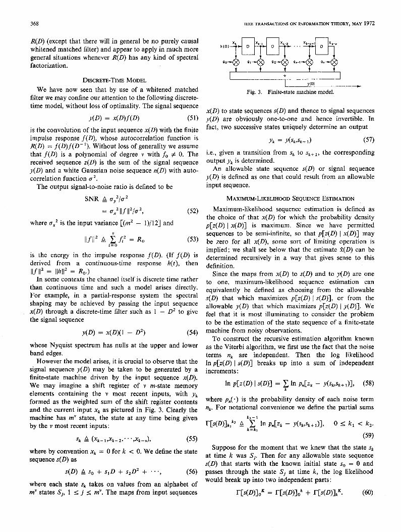
t t t t t + I y(D)

Fig. 3. Finite-state machine model.

Y(D) = xVW-(9 (51)

is the convolution of the input sequence x(D) with the finite impulse response f(D), whose autocorrelation function is R(D) = f(D)f(D-I). Without loss of generality we assume that f(D) is a polynomial of degree v with f. # 0. The received sequence z(D) is the sum of the signal sequence y(D) and a white Gaussian noise sequence n(D) with autocorrelation function (T 2.

x(D) to state sequences s(D) and thence to signal sequences y(D) are obviously one-to-one and hence invertible. In fact, two successive states uniquely determine an output

yk = YbkTsk+ 1) (57)

i.e., given a transition from s, to s~+~, the corresponding output y, is determined.

The output signal-to-noise ratio is defined to be

SNR A (ry2/a2

= ox2 Ilf l12/02, where 6, 2 is the input variance [(m’ - 1)/12] and

(52)

An allowable state sequence s(D) or signal sequence y(D) is defined as one that could result from an allowable input sequence.

MAXIMUM-LIKELIHOOD SEQUENCE ESTIMATION

Maximum-likelihood sequence estimation is defined as the choice of that x(D) for which the probability density p[z(D) I x(D)] is maximum. Since we have permitted sequences to be semi-infinite, so that p[z(D) I x(D)] may be zero for all x(D), some sort of limiting operation is implied; we shall see below that the estimate 2(D) can be determined recursively in a way that gives sense to this definition.

Ml2 B i$oL2 = Ro

is the energy in the impulse response f(D). (If f(D) is derived from a continuous-time response h(t), then Ilf II2 = llhl12 = Ro.1

In some contexts the channel itself is discrete time rather than continuous time and such a model arises directly. For example, in a partial-response system the spectral shaping may be achieved by passing the input sequence x(D) through a discrete-time filter such as 1 - D2 to give the signal sequence

y(D) = x(D)(l - D2) (54)

whose Nyquist spectrum has nulls at the upper and lower band edges.

However the model arises, it is crucial to observe that the signal sequence y(D) may be taken to be generated by a finite-state machine driven by the input sequence x(D). We may imagine a shift register of v m-state memory elements containing the v most recent inputs, with y, formed as the weighted sum of the shift register contents and the current input xk as pictured in Fig. 3. Clearly the machine has my states, the state at any time being given by the v most recent inputs:

sk g (xk-l,xk-2; ’ ‘,xk-v), (55)

where by convention xk = 0 for k < 0. We define the state sequence s(D) as

s(D) p so + s,D + s2D2 + . . . . (56)

where each state Sk takes on values from an alphabet of my states Sj, 1 I j I my. The maps from input sequences

Since the maps from x(D) to s(D) and to y(D) are one to one, maximum-likelihood sequence estimation can equivalently be defined as choosing from the allowable s(D) that which maximizes p[z(D) 1 s(D)], or from the allowable y(D) that which maximizes p[z(D) I y(D)]. We feel that it is most illuminating to consider the problem to be the estimation of the state sequence of a finite-state machine from noisy observations.

To construct the recursive estimation algorithm known as the Viterbi algorithm, we first use the fact that the noise terms nk are independent. Then the log likelihood lnp[z(D) I s(D)] breaks up into a sum of independent increments :

In dz(D) I s(D)1 = F In dZk - Y(sk,sk+l)l, (58)

where p,( *) is the probability density of each noise term n,+. For notational convenience we define the partial sums

kz-1

rb(D)],,k2 Li c k=k,

Suppose for the moment that we knew that the state 8, at time k was Sj. Then for any allowable state sequence s(D) that starts with the known initial state so = 0 and passes through the state Sj at time k, the log likelihood would break up into two independent parts:

In dZk - Y@kpsk+ l>l? 0 I k, < k2.

(59)

rb(D)loK = rb(D)]ok + r[@)]?. WV

FORNEY : MAXIMUM-LIKELIHOOD SEQUENCE ESTIMATION

Let S,(D) be the allowable state sequence from time 0 to k that has m inimum log likelihood T[s(D)lok among all allowable state sequences starting with so = 0 and ending with sk = Sj. We call 3j(D) the survivor at time k corresponding to state Sj. Then we assert that S,(D) must be the initial segment of the maximum likelihood state sequence s(D); for we can replace the initial segment s’(D) of any allowable state sequence passing through Sj with the initial segment 3,(D) and obtain another allowable sequence with greater log likelihood T[s(D)]oK, unless r[s’(D)lok = r[3j(D)lok.

In fact, we do not know the state s, at time k; but we do know that it must be one of the finite number of states Sj, 1 I j < my, of the shift register of F ig. 3. Consequently, while we cannot make a final decision as to the identity of the initial segment of the maximum-likel ihood state sequence at time k, we know the initial segment must be among the my survivors 3j(D), 1 I j < my, one for each state Sj. Thus we need only store my sequences S,(D) and their log likelihoods r[sj(D)lok, regardless of how large k becomes. To update the memory at time k + 1, recursion proceeds as follows.

1) For each of the m allowable continuations sjS(D) to time k + 1 of each of the my survivors S,(D) at time k compute r[sj'(D)]kg+l = r[3j(D)]ok + In p,[ zk - Yk(sj,sj’>l* (61)

This involves rn” ’ = mL additions. 2) For each of the states S,,, 1 < j’ _< my, compare the

log likelihoods r[sjP(D)lo k+l of the m continuations termin- ating in that state and select the largest as the corresponding survivor. This involves my m-ary comparisons, or (m - 1) my binary comparisons.

In principle the Viterbi algorithm can make a final decision on the initial state segment up to time k - T when and only when all survivors at time k have the same initial state sequence segment up to time k - z. The decoding delay r is unbounded but is generally finite with probability 1 [34]. In implementation, one actually makes a final decision after some fixed delay 6, with 6 chosen large enough that the degradat ion due to premature decisions is negligible. Although, as we shall see later, 6 may have to be much larger than v, it is typically of the order of 20 symbols or less. Parenthetically, our analysis following shows that the capability of deferring decisions is essential, in the sense that any receiver that does not have the capability of deferring decisions for the appropriate 6 cannot approach opt imum performance.

We further note that in the derivation of the algorithm we have used only the finite-state machine structure and the independence of the noise, so that the technique can be adapted to account for Markov context dependence in the input and other Markov-modelable statistics of the source and channel, as recounted by Hilborn [16], for example. Omura [30] has considered the situation in which the input sequence x(D) is a code word from a convolutional code.

369

ERROR EVENTS

We now begin our analysis of the probability of error in the estimated state sequence 3(D) finally decided upon by the Viterbi algorithm. We let A(D) and j(D) stand for the corresponding estimated input sequence and signal sequence.

In the detection of a semi-infinite sequence there will generally occur an infinite number of errors. The idea of error events (see also [20] and [28]) makes precise our intuitive notion that these errors can be grouped into independent finite clumps. An error event d is said to extend from time k, to k, if the estimated state sequence 3(D) is equal to the correct state sequence s(D) at times k, and k,, but nowhere in between (sk, = d,, ; sk2 = s*,,; Sk # dk, k, < k < k2). The length of the error event is defined as n B k, - k, - 1. Clearly n 2 v, with no upper bound; however, we shall find that n is finite with probability 1.

When the channel is linear, in the sense that y(D) = x(D)f(D), we can say more about an error event. Since % = Sk, and Sk2 = $k2) we have

xk = gk, k,-v<k<k,-1

k,-vIkIk2-1

from the definition of s,. However, xk, # xkl-v-l # j2kl-v-l since skl+l # 3kl+l and sk2-l We define

E,(D) A cxk, - ak,> + cxk, + I - fk,+ N + ’ ’ ’

(62) 2 and &,,-1.

+ (xk2-,,-l - &2-v-1)D"-v (63)

as the input error sequence associated with the error event. It is a polynomial with nonzero constant term .sXO and degree n - v and contains no sequence of v consecutive zero Coefficients (Since then sk would equal $k for some intermediate k and we would have two distinct error events). Furthermore, since the xk are integers, the coefficients of E,(D) are integral.

Correspondingly, we define the signal error sequence associated with the error event as

E,@) ii (yk, - Pk,) + (yk,+ I - $k,+ IV’ + ’ ’ ’

+ (Yk,-1 - $kz-l)D”. (64) Since y(D) = x(D)f(D) and j(D) = ,?(D)f(D), it follows that

&y(D) = GW-(D). (65) Thus E,,(D) is a polynomial with nonzero constant term and degree n.

We define the Euclidean weight d2(6) of an error event as the energy in the associated signal-error sequence

d’(~) ~ lleyJ12 = ~ Eyi2 i=O

= by(D)-@- ‘110 = C @ M W W lMD- ‘>I0 = C M W W M D - ‘>I 0.


We note that the energy depends only on a%(D) and R(D) and is therefore independent of the factorization R(D) = f(D)f(D-I). In fact, when the received sequence is derived from a continuous-time received signal via a whitened matched filter, d’(E) is identifiable as the energy of the signal that results from passing the sequence E,(D) through h(t):

= 1 [I$: E,ih(t - i7)12 dt. (67)

The number of errors in the associated input error sequence is defined as the Hamming weight ~~(8) of the event; that is,

w,(b) P number of nonzero coefficients in E,(D). (68)

PROBABILITYOFA PARTICULAR ERROR EVENT the Euclidean distance between y(D) and j(D). But since We now calculate the probability that a particular error

event identified by a starting time k, and an associated input error sequence E,(D) of degree 12 - v will actually occur. Three subevents must occur.

8,: At time k, we must have sk, = gkl. 8,: Between k, and k, + n - v the input sequence

x(D) must be such that x(D) + E,(D) is an allowable sequence J(D). For example, if E,(D) = 1, then xkl must not equal m - 1, since then Akl would equal m, which is not an allowable level.

8,: The noise terms nk, k, I k < k, + n, must be such that over this segment a(D) has greater likelihood than x(D) or, in terms of the earlier notation of (59),

r[qD)];; +lz+ l 2 I-[s(D)]:: +“+I. (69) When n(D) is white and Gaussian with variance a2,

we have

In p,(zk - yk) = -3 In 27co’ - (z, - yk)2/2a2 (70)

so that

[F - I-]::+n+l = $ I$” [(Zk - y/J2 - (Zk - $&“I 1

= & [IW) - Y(~)I12

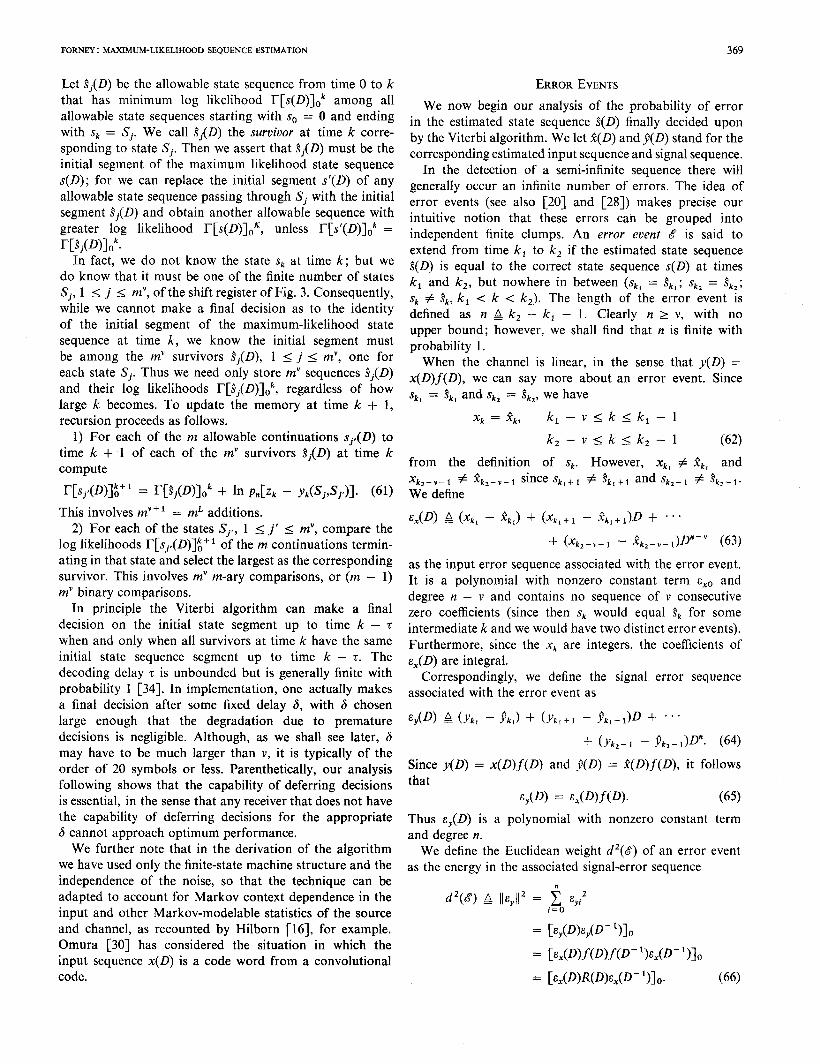
- IW) - 9ml121~:+” (71) in obvious notation. In words, j(D) is more likely than y(D) if j(D) is closer to z(D) than is y(D) in the (n + l)- dimensional Euclidean space corresponding to times k, to k, + 12. (The decision rule is thus independent of signal- to-noise ratio.) The three points

Y(D) I ;: + “7 P(D) I !4:+7 z(D) I ::+”

QD) = [Y(D) - P<D)lt:+” this distance squared is just the Euclidean weight d’(&‘) of cy(D). Hence

m Pr (g3) = s

dn(2x02)-1/2 exp - n2/2a2 d(Ql2

= 'Q[d<~>P~l, (72)

where Q(x) is defined in (4). We recognize this as the error probability when a binary signal of amplitude &d(b)/2 is sent through a Gaussian channel with noise variance 02. It depends only on c,,(D) and 0.

The subevent 6, is independent of 8, and d,, being dependent only on the message ensemble. Clearly when lsxil = j only m - j values of xk+ i are permissible, so that

(73)

assuming the inputs to be independent and equiprobable. Error events with any l&xi1 2 m are impossible.

The subevent 8, is possibly dependent on the noise terms involved in 8, and the joint probability is not easily calculable. However, the probability that 8, is not true is of the order of the error probability, so that in the normal operating region Pr (8, 1 8,) is closely approximated as well as overbounded by 1. In sum, therefore, the probability of the particular error event d is given by

Pr (E) = Pr (8,) Pr (g2) Pr (6, 1 8,)

5 Q[d(S)/2c] ;n; ” -m’“xi’] . (74)

define a two-dimensional subspace illustrated in Fig. 4. PROBABILITYOFERROR

Since our Gaussian noise has equal variance in all dimen- From the probabilities of individual error events we sions, it is spherically symmetric and by coordinate rotation obtain a simple and, for moderately low error probabilities we can see that the probability of 8, is simply the probability like 10w3, rather tight bound on overall probability of error that a single Gaussian variable of variance a2 exceeds half through the union bound, which simply says that the prob-


ability of a union Ff events is not greater than the sum of their individual probabilities.

Let E be the set of all possible error events &’ starting at time k,. Then the probability that any error event starts at time k, is bounded by

Pr (El I JE Pr (0 (75)

Let D be the set of all possible d(b) and for each d E D let Ed be the subset of error events for which d(b) = d. Then from (74)

Pr (E) I C Q[d/2a] C [IDi ssi’] . (76) dsD ICEEd

Because of the exponential decrease of the Gaussian distribution function, this expression will be dominated at moderate signal-to-noise ratios by the term involving the m inimum value dmin of d(b):

where (77)

1 (78)

is a constant independent of CF. Since this expression is independent of k,, it may be read as the probability of an error event per unit time, and its reciprocal l/Pr (E) as the mean time between error events. The size of the signal- to-noise ratio at which this expression becomes a good estimate depends on the coefficients of Q[d(&‘)/2o] for larger d(b), which in all cases we examine are of the order of magn itude of Ki.

A true bound with the same asymptotic behavior can be obtained by generating-function methods similar to those used by Viterbi [21]. Let Nd be the coefficient mu ltiplying Q[d/2a] in (76) and let the generat ing function g,,,(z) be defined as

&V(Z) 6 c NdZd2. (79) dsD

As suggested by Viterbi in [21], we use the fact that Q(x) exp x2/2 is a monotonically decreasing function of x for x 2 0 to obtain the bound

Q[d/20] 5 Q[dmiJ20] exp (d&n - d2)/802, (80)

which can be substituted in (76) to obtain the upper bound

Pr (E) I C NdQ[d,i”/2a] exp (d&n - d2)/802 dsD

= Q[dm~n/2~]{~dm~n2’80z~~(~~1’8u2)}. (81)

As r~ + 0 the expression in brackets approaches Nd-.- = K, .

Pr (e) < C w,(b) Pr (8) 8sE

I d;D QCdPl c w,(b) dEEd

(82)

where

K24 c wHc8j “fi m -ml&~il 1 (83)

8 E f&in i=O

is another constant independent of CT. The quantity K,/K, may be interpreted as the average number of symbol errors per error event at high signal-to-noise ratios.

Obviously the average of any variable that is a finite function of error events (e.g., the average length of error events, the bit error probability, etc.) can be calculated in the same way. In each case we can approximate the result by a constant mu ltiplied by Q[d,,J2a] for sufficiently high signal-to-noise ratios. Strict upper bounds like (81) can also be obtained by the f low-graph techniques of [21] as we indicate in Appendix I.

The obvious lower bound shows that these bounds and estimates are very tight. Let Edmin be the set of error events E,(D) of Euclidean weight dmi, and let K. I 1 be the probability that the input sequence x(D) will be such that A(D) = x(D) + ok&,(D) is an allowable input sequence for at least one E,(D) E Edmin. When diin = Ilfl12, Edmin contains E,(D) = & 1, so Ko = 1. The probability that such an a(D) will be closer than x(D) to the received sequence z(D) is Q[d,,,,,/2g]. Hence, with probability K,, the probability of an error event starting at time k for any k is at least Q[d,,,J2g], so

Pr (El 2 &Q[4ninP~I Pr (4 2 KoQ[4nin/2~I* (84)

Thus the upper estimate and lower bound differ only in their constant coefficient. Applications of this lower bound are given in [38].

If the channel were used for only one pulse, i.e., xk = 0 for k # 0, then intersymbol interference would be absent, the signal sequence would be of the form

Y(D) = xof(D) (85)

and the symbol-error probability would be very nearly

Pr (4 = &Q< Ilf W W 3 (86)

where K3 = 2(m - 1)/m. This gives a slightly tighter version of the lower bound above when 1lflI” = dzi”.

It also suggests that we define the effective signal-to-noise ratio as

SNR,,, & rsx2d;,Jo ‘, (87) ....ll

Evaluation of this bound involves finding the generat ing where again ox2 = (m’ - 1)/12, for (82) and (86) then function, which in general can be done through flow-graph show that the probability of error of an m-level PAM techniques [21], illustrated in Appendix I. system with intersymbol interference differs at most by the

The symbol probability of error Pr (e) may be similarly ratio K2/K3 from that of an m-level system without inter- computed by weighting each error event & by the number symbol interference and output signal-to-noise ratio SNR,,,. of decision errors w,(b) it entails: In decibels such a difference is small and goes to zero as


SNR,,, goes to infinity. But in the common case when Ilf II” = &in, SNR equals SNR,,,, so that the degradation due to intersymbol interference is negligible. This result, while conjectured in [ 151, seems effectively unanticipated in the intersymbol interference and partial-response literature. In particular, partial-response techniques had been thought to cost at least 3 dB in output SNR, whereas we see in the following (see also [33]) that for f(D) = 1 + D” the penalty in SNR with the Viterbi algorithm is a small fraction of a decibel.

Upon a little reflection, we are not surprised that when the only constraint is on the output signal-to-noise ratio’ no degradation need be suffered because of intersymbol interference; for we could simply choose the output sequences y(D) to suit our purposes within the constraint and let x(D) = y(D)/‘(D). That the inputs xk would become very large if f(D) had an unstable inverse’ m ight bother us physically, but not mathematically. The surprising result is that under the rigid constraint that the inputs xk be m equally spaced amplitudes, we can do nearly as well when llj” 11” = d&.

When llfl12 > d,$,, which tends to happen when intersymbol interference is severe, the ratio SNRJSNR is d~i”/Ilf 11’ and measures the degradation due to intersymbol interference. We show in Appendix II that even in this case degradation can be avoided if it is permissible to insert a certain type of partial-response preemphasis filter at the transmitter.

EXAMPLE : PARTIAL RESPONSE

Let f(D) = 1 - D. (Everything that follows also holds with the obvious modifications for any partial response of the form 1 + D”.)

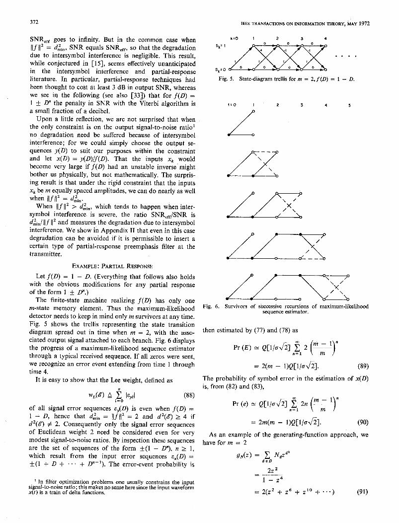
The finite-state machine realizing f(D) has only one m-state memory element. Thus the maximum-likelihood detector needs to keep in m ind only m survivors at any time. Fig. 5 shows the trellis representing the state transition diagram spread out in time when m = 2, with the associated output signal attached to each branch. Fig. 6 displays the progress of a maximum-likelihood sequence estimator through a typical received sequence. If all zeros were sent, we recognize an error event extending from time 1 through time 4.

It is easy to show that the Lee weight, defined as

WL@Y P j. IQI (88)

of all signal error sequences cy(D) is even when f(D) = 1 - D, hence that d& = Ilfl12 = 2 and d’(6) 2 4 if d2(8) # 2. Consequently only the signal error sequences of Euclidean weight 2 need be considered even for very modest signal-to-noise ratios. By inspection these sequences are the set of sequences of the form -l-(1 - D”), n 2 1, which result from the input error sequences E,(D) = +(l + D + *.a + D.-l). The error-event probability is

1 In filter optimization problems one usually constrains the input signal-to-noise ratio; this makes no sense here since the input waveform x(t) is a train of delta functions.

Fig. 5. State-diagram trellis for m = 2,f(D) = 1 - D.

I:0 I 2 3 4 5

& -- \ n \

Fig. 6. Survivors of successive recursions of maximum-likelihood sequence estimator.

then estimated by (77) and (78) as

Pr (E) N Q[l/a&] 2 2 (v)” n=l

= 2(m - l)Q[l/o&]. (89) The probability of symbol error in the estimation of x(D) is, from (82) and (83),

Pr (e) N Q[l/a&] 2 2n (5 n=l

= 2m(m - l)Q[l/o&].

As an example of the generating-function have for m = 2

gN@) = c NdZd2 deD

2z2 1 - z4

(90) approach, we

= 2(z2 + z6 + z10 + *em) (91)

FORNEY : hfAXIMUM-LIKELIHOOD SEQUENCE FSITMATION

as is shown by f low-graph techniques in Appendix I. This means that there are error events of Euclidean weights 2,6,10, * * *, and that the coefficient of each weight is 2. We obtain the strict upper bound

(92)

The accuracy of approximating the series (76) by its first term even for r~ of the order of 1 is evident.

Preceding is a technique that has been used in partial response systems to prevent infinite error propagat ion in recovery of the transmitted sequence. As we have seen, with maximum-likel ihood sequence estimation error events are quite finite; even so, preceding is useful in reducing symbol-error probability when m > 2. The idea [I], [3] is to take the original m-ary sequence, which we now call d(D), and let the input sequence be another m-ary sequence defined by

x(D) 4 d(D)/f(D) modu lo m, (93)

which is well-defined when f(D) = 1 If: D” (or more generally when f0 and m are relatively prime). Then if we could take the output sequence modu lo m we would obtain

y(D) = x(D)f(D) = d(D) modu le m. (94)

In fact, we obtain the estimated data sequence d(D) by the zero-memory modu lo-m operation on p(D) :

d(D) b E(D) modu lo m. (95)

The number of symbol errors in d(D) is therefore the same as the number of nonzero coefficients in cy(D). Forf(D) = 1 rf: D”, this number is 2 for all the E,,(D) of weight 2, which is to say that with preceding all the likely error events result in 2 symbol errors in the estimation of d(D). Hence

Pr (e) N 2 Pr (E) N 4(m - l)Q[l/oJZ]. (96)

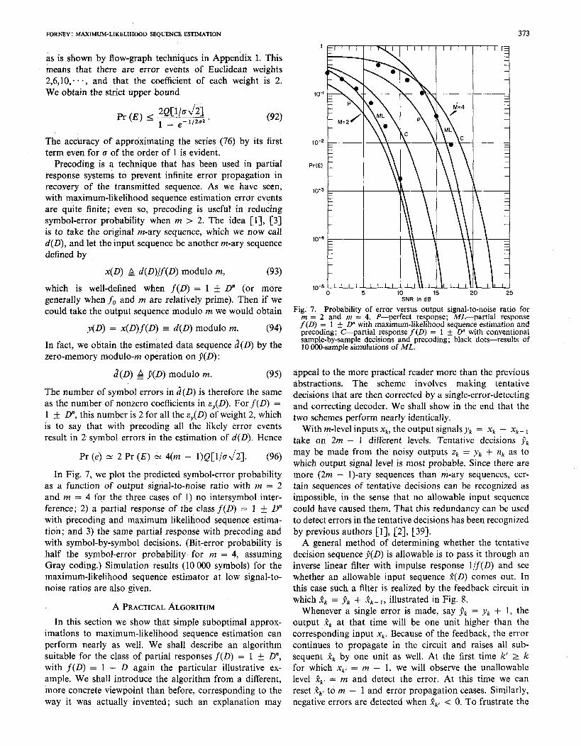
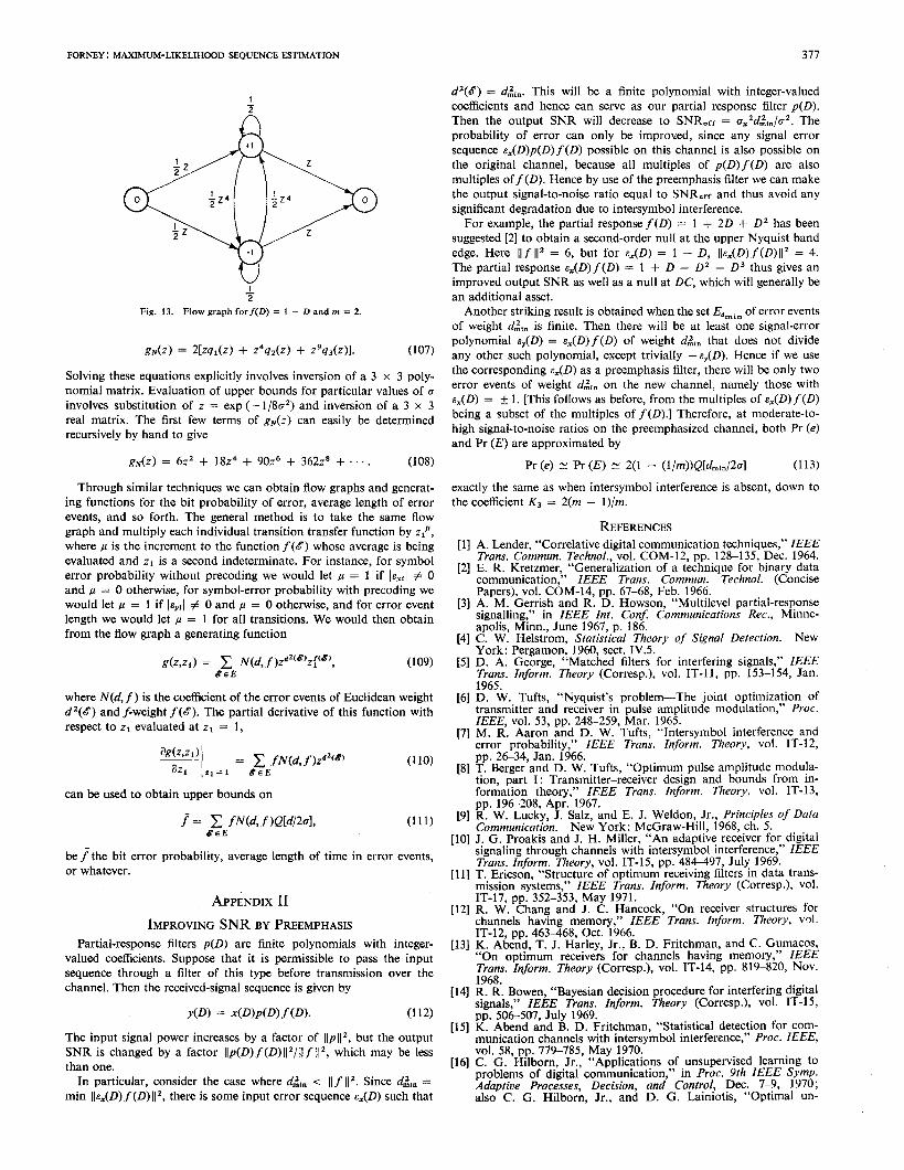
In F ig. 7, we plot the predicted symbol-error probability as a function of output signal-to-noise ratio with m = 2 and m = 4 for the three cases of 1) no intersymbol interference; 2) a partial response of the class f(D) = 1 _+ D” with preceding and maximum likelihood sequence estimation; and 3) the same partial response with preceding and with symbol-by-symbol decisions. (Bit-error probability is half the symbol-error probability for m = 4, assuming Gray coding.) Simulation results (10 000 symbols) for the maximum-likel ihood sequence estimator at low signal-to- noise ratios are also given.

A PRACTICAL ALGORITHM

In this section we show that simple suboptimal approx- imations to maximum-likel ihood sequence estimation can perform nearly as well. We shall describe an algorithm suitable for the class of partial responses f(D) = 1 + D”, with f(D) = 1 - D again the particular illustrative ex- amp le. We shall introduce the algorithm from a different, more concrete viewpoint than before, corresponding to the way it was actually invented; such an explanation may

0 5 IO 15 20 25 SNR in dB

Fig. 7. Probability of error versus output signal-to-noise ratio for m = 2 and m = 4. P-perfect response; ML-partial response f (0) = 1 I!Z D” with maximum-likel ihood sequence estimation and preceding; C-partial response f(D) = 1 f D” with conventional sample-by-sample decisions and preceding; black dots-results of 10 000-sample simulations of ML.

appeal to the more practical reader more than the previous abstractions. The scheme involves making tentative decisions that are then corrected by a single-error-detecting and correcting decoder. We shall show in the end that the two schemes perform nearly identically.

W ith m-level inputs xk, the output signals yk = xk - xk- 1 take on 2m - 1 different levels. Tentative decisions j$ may be made from the noisy outputs zk = yk + nk as to which output signal level is most probable. Since there are more (2m - I)-ary sequences than m-ary sequences, certain sequences of tentative decisions can be recognized as impossible, in the sense that no allowable input sequence could have caused them. That this redundancy can be used to detect errors in the tentative decisions has been recognized by previous authors [1], [2], [39].

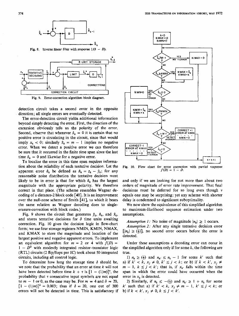
A general method of determining whether the tentative decision sequence J(D) is allowable is to pass it through an inverse linear filter with impulse response l/f(D) and see whether an allowable input sequence a(D) comes out. In this case such a filter is realized by the feedback circuit in which & = j& + $ _ 1, illustrated in F ig. 8.

Whenever a single error is made, say J$ = yk + I, the output 12, at that time will be one unit higher than the corresponding input xk. Because of the feedback, the error continues to propagate in the circuit and raises all sub- sequent 5~~ by one unit as well. At the first time k’ 2 k for which xk, = m - 1, we will observe the unallowable level R,, = m and detect the error. At this time we can reset jz,, to m - 1 and error propagat ion ceases. Similarly, negative errors are detected when & < 0. To frustrate the


Fig. 8. Inverse linear filter with response l/(1 - 0).

8 -UNIT STORAGE

TENTATIVE DECEIONS

9, & CORRECTIONS

CORRECTION CIRCUIT

Fig. 9. Error-correction algorithm block diagram.

detection circuit takes a second error in the opposite direction; all single errors are eventually detected.

The error-detection circuit yields additional information beyond simply detecting the error. First, the direction of the excursion obviously tells us the polarity of the error. Second, observe that whenever II, = 0 it is certain that no positive error is circulating in the circuit, since that would imply x, < 0; similarly R, = m - 1 implies no negative error. When we detect a positive error we can therefore be sure that it occurred in the finite time span since the last time Rk = 0 and likewise for a negative error.

To localize the error in this time span requires information about the reliability of each tentative decision. Let the apparent error R, be defined as Ak = z, - j&; for any reasonable noise distribution the tentative decision most likely to be in error is that for which Ak has the largest magnitude with the appropriate polarity. We therefore correct in that place. (The scheme resembles Wagner decoding of a distance-2 block code [40]. It is an improvement over the null-zone scheme of Smith [41], to which it bears the same relation as Wagner decoding does to single- erasure-correction with block codes.)

Fig. 9 shows the circuit that generates JJ,, Ak, and &, and stores tentative decisions for S time units awaiting correction, Fig. 10 gives the decision logic in flow-chart form; we use four storage registers NMIN, KMIN, NMAX, and KMAX to store the magnitude and location of the largest positive and negative apparent errors. To implement an equivalent algorithm for m = 2 or 4 with f(D) = 1 - D* with modestly integrated resistor-transistor logic (RTL) circuits (2 flip/flops per IC) took about 50 integrated circuits, including all control logic.

To determine how long the storage time 6 should be, we note that the probability that an error at time k will not have been detected before time k + 7 is [l - (i/m)]‘, the probability that z consecutive input symbols are not equal to m - 1 or 0, as the case may be. For m = 4 and 6 = 20, [l - (l/m)]” = 0.003; thus if 6 = 20, one out of 300 errors will not be detected in time. This is satisfactory if

NO -I ERROR c N MAX=0

CORRECT + I

CORRhT-1

. . . . . . .

k=ktl

Fig. 10. Flow chart for error correction with partial response f(D) = 1 - D.

and only if we are looking for not more than about two orders of magnitude of error rate improvement. That final decisions must be deferred for so long even though v equals one may be surprising; yet any scheme with shorter delay is condemned to significant suboptimality.

We now show the equivalence of this simplified algorithm to maximum-likelihood sequence estimation under two assumptions.

Assumption 2: No noise of magnitude InkI 2 1 occurs. Assumption 2: After any single tentative decision error

l$klc~~~n no second error occurs before the error is

Under these assumptions a decoding error can occur in the simplified algorithm only if for some k, the following are true.

1) nk 2 (4) and nkP I nk - 1 for some k’ such that a) if k’ < k, Xj # 0, k’ 5 j < k; or b) if k < k’, Xj # m - 1, k I j < k’ ; that is, if x,, falls within the time span in which the error could have occurred when the error in x, is detected.

2) Similarly, if nk I -(JJ and n,, 2 1 + nk for some k’ such that a) if k’ < k, xi # m - 1, k’ I j < k; or b) if k < k’, Xj # 0, k I j < k’.


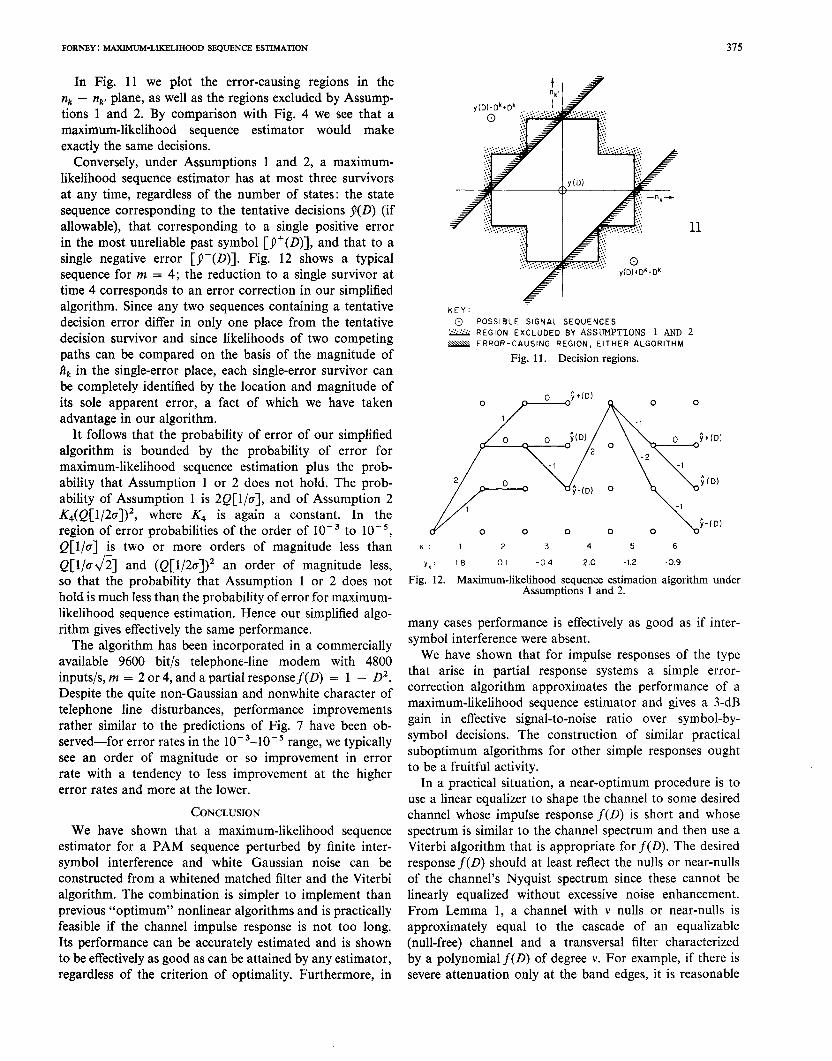
In F ig. 11 we plot the error-causing regions in the nk - &’ plane, as well as the regions excluded by Assump- tions 1 and 2. By comparison with F ig. 4 we see that a maximum-likel ihood sequence estimator would make exactly the same decisions.

Conversely, under Assumptions 1 and 2, a maximum- likelihood sequence estimator has at most three survivors at any time, regardless of the number of states: the state sequence corresponding to the tentative decisions g(O) (if allowable), that corresponding to a single positive error in the most unreliable past symbol [j’(O)], and that to a single negative error [j-(O)]. F ig. 12 shows a typical sequence for m = 4; the reduction to a single survivor at time 4 corresponds to an error correction in our simplified algorithm. Since any two sequences containing a tentative decision error differ in only one place from the tentative decision survivor and since likelihoods of two competing paths can be compared on the basis of the magn itude of fik in the Single-error place, each single-error survivor can be completely identified by the location and magn itude of its sole apparent error, a fact of which we have taken advantage in our algorithm.

11

KEY: 0 POSSIBLE SIGNAL SEOUENCES

22 REGION EXCLUDED BY ASSUMPTIONS 1 AND 2 m ERROR-CAUSING REGION, EITHER ALGORITHM

Fig. 11. Decision regions.

It follows that the probability of error of our simplified algorithm is bounded by the probability of error for maximum-likel ihood sequence estimation plus the probability that Assumption 1 or 2 does not hold. The probability of Assumption 1 is 2Q[l/a], and of Assumption 2 &@Cw~lK where K4 is again a constant. In the region of error probabilities of the order of 10m3 to lo-‘, Q [l/c] is two or more orders of magn itude less than Q[l/~h] and (Q[W a ])’ an order of magn itude less, so that the probability that Assumption 1 or 2 does not hold is much less than the probability of error for maximum- likelihood sequence estimation. Hence our simplified algorithm gives effectively the same performance.

The algorithm has been incorporated in a commercially available 9600 bit/s telephone-l ine modem with 4800 inputs/s, m = 2 or 4, and a partial responsef(l)) = 1 - D2. Despite the quite non-Gaussian and nonwhite character of te lephone line disturbances, performance improvements rather similar to the predictions of F ig. 7 have been ob- served-for error rates in the 1O-3-1O-5 range, we typically see an order of magn itude or so improvement in error rate with a tendency to less improvement at the higher error rates and more at the lower.

CONCLUSION

We have shown that a maximum-likel ihood sequence estimator for a PAM sequence perturbed by finite intersymbol interference and white Gaussian noise can be constructed from a whitened matched filter and the Viterbi algorithm. The combination is simpler to implement than previous “opt imum” nonlinear algorithms and is practically feasible if the channel impulse response is not too long. Its performance can be accurately estimated and is shown to be effectively as good as can be attained by any estimator, regardless of the criterion of optimality. Furthermore, in

k 1 2 3 4 5 6

yk: 18 01 -04 2.0 -1.2 -0.9

Fig. 12. Maximum-likel ihood sequence estimation algorithm under Assumptions 1 and 2.

many cases performance is effectively as good as if intersymbol interference were absent.

We have shown that for impulse responses of the type that arise in partial response systems a simple error- correction algorithm approximates the performance of a maximum-likel ihood sequence estimator and gives a 3-dB gain in effective signal-to-noise ratio over symbol-by- symbol decisions. The construction of similar practical subopt imum algorithms for other simple responses ought to be a fruitful activity.

In a practical situation, a near-opt imum procedure is to use a linear equalizer to shape the channel to some desired channel whose impulse response f(o) is short and whose spectrum is similar to the channel spectrum and then use a Viterbi algorithm that is appropriate for f(o). The desired responsef(D) should at least reflect the nulls or near-nulls of the channel’s Nyquist spectrum since these cannot be linearly equal ized without excessive noise enhancement. From Lemma 1, a channel with v nulls or near-nulls is approximately equal to the cascade of an equalizable (null-free) channel and a transversal filter characterized by a polynomialf(D) of degree v. For example, if there is severe attenuation only at the band edges, it is reasonable


to choose f(D) = 1 - D2. Analysis of how close one can come to optimal performance with this approach would be useful.

Another practical problem is that the channel response h(t) is usually unknown, so that the receiver must be adaptive. In the approach of the previous paragraph, one can obviously make the linear equalizer the adaptive element. It would be of interest, however, to devise an adaptive version of the maximum-likelihood sequence estimator itself.

On the theoretical side, the greatest deficiency in our results is their reliance on a finite channel response. It can be shown that the brute-force approach of approximating an infinite response by a truncated response of length L and then using the appropriate sequence estimator gives performance that is accurately estimated by (77) and (82) as L + cc, where d,$,, is still defined as min Ils,(D)f(D)l12 for the true (infinite) f(D). There must be a better way, however, of dealing with simple infinite responses like h(t) = e --f/1, t 2 0.

These results can be extended in a number of directions.

where .a is an indeterminate. Then with any particular path (error event) from the initial node to the final node is associated the transfer function

We recognize I: eYr2 as d”(l), the Euclidean weight of the error event. Hence the total transfer function of the flow graph, which is the sum of the transfer functions of all paths, is simply

Extension to quadrature PAM, where phase as well as amplitude is modulated, is achieved straightforwardly by letting the input sequence x(D) be complex, although the analysis is slightly complicated by having to deal with complex E,(D). Colored noise can be handled by pre- whitening. The possibility of extensions to handle context- dependent x(D) and other Markov-modelable constraints has already been mentioned. Finally, the use of similar techniques outside digital communications (for example, in magnetic-tape reading [32]) will no doubt be extensive.

ACKNOWLEDGMENT

It is a pleasure to acknowledge the kind interest and help- ful comments of J. L. Massey and R. Price.

Clearly, from the linearity of PAM, the input errors eXl govern the state-error transitions and the signal errors ey, are functions of gXl and Q, or eqmvalently of E,~ and a.,r+ r.

An error event starts and ends with an all-zero state error. From the input error sequence E@) we can determine the path taken through the nonzero state error sequences during the error event. Each possible error event thus corresponds to a unique such path.

Let us then construct a flow diagram in which the initial node is the all-zero state error, the intermediate nodes are the nonzero state errors, and the final node is again the all-zero state error. Let us draw in all possible state-error transitions and label each with the corresponding .Q and Q. To each transition we assign a weight or transfer function equal to

(101)

the desired generating function. In simple cases, one can solve the flow graph fairly easily to obtain

an explicit expression for g,,(z). In more complicated cases, one may merely solve the flow graph modulo z” for small values of n to determine the coefficients Nd for dZ < n; or one may solve for particular real number values of z to determine the tightness of the asymptotic expressions.

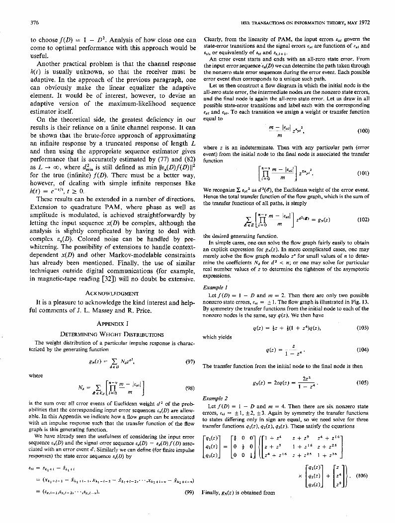
Example 1 Let f(D) = 1 - D and m = 2. Then there are only two possible

nonzero state errors, csl = k 1. The flow graph is illustrated in Fig. 13. By symmetry the transfer functions from the initial node to each of the nonzero nodes is the same, say q(z). We then have

APPENDIX I

DETERMINING WEIGHT DISTRIBUTIONS which yields q(z) = fz + $0 + z‘Yq(z), (103)

The weight distribution of a particular impulse response is characterized by the generating function q(z) = + . (104)

gn(z) = c Ncd2, (97) deD The transfer function from the initial node to the final node is then

where

I (98)

is the sum over all error events of Euclidean weight d2 of the probabilities that the corresponding input error sequences E,(D) are allowable. In this Appendix we indicate how a flow graph can be associated with an impulse response such that the transfer function of the flow graph is this generating function.

Example 2 Let f(D) = 1 - D and m = 4. Then there are six nonzero state

errors, E,* = k 1, + 2, + 3. Again by symmetry the transfer functions to states differing only in sign are equal, so we need solve for three transfer functions qI(z), q2(z), q3(z). These satisfy the equations

We have already seen the usefulness of considering the input error sequence EJD) and the signal error sequence EJD) = c,(D)f(D) associated with an error event 8. Similarly we can define (for finite impulse responses) the state error sequence es(D) by

E ri = s!q+i - &,ff (x . (106) = kl+l-l - *k~+l-l,&,+1-2 - &,+i--2,“‘,xk~+l-v- xkl+l-” )

= (&.l- 1&x.i-2,‘. ‘,&c,l-” 1 . (99) Finally, gN(z) is obtained from

FORNEY : MAXIMUM-LIKELIHOOD SEQUENCE ESTIMATION 377

+ Fig. 13. Flow graph forf(D) = 1 - D and m = 2.

&f(z) = 2kl(Z) + z%(z) + zPq3(z)1. (107)

Solving these equat ions explicitly involves inversion of a 3 x 3 polynomial matrix. Evaluation of upper bounds for particular values of 0 involves substitution of z = exp (- l/8u2) and inversion of a 3 x 3 real matrix. The first few terms of gN(z) can easily be determined recursively by hand to give

gpg(z) = 6z2 + 18z4 + 90z6 + 362~~ + . . . . (108)

Through similar techniques we can obtain flow graphs and generating functions for the bit probability of error, average length of error events, and so forth. The general method is to take the same flow graph and multiply each individual transition transfer function by zip, where p is the increment to the function f(g) whose average is being evaluated and zi is a second indeterminate. For instance, for symbol error probability without preceding we would let p = 1 if I&xi] # 0 and p = 0 otherwise, for symbol-error probability with preceding we would let /I = 1 if J+] # 0 and p = 0 otherwise, and for error event length we would let p = 1 for all transitions. W e would then obtain from the flow graph a generat ing function

g(z,z1) = c N(d,f)ZdZ(g)Z:(g), 8EE

where N(d, f) is the coefficient of the error events of Eucl idean weight d*(e) and f-weight f(g). The partial derivative of this function with respect to z1 evaluated at z1 = 1,

can be used to obtain upper bounds on

j = C fN(d,.fMW~l, 8eE

(111)

be fthe bit error probability, average length of time in error events, or whatever.

APPENDIX II IMPROVING SNR BY PREEMPHASIS

Partial-response filters p(D) are finite polynomials with integer- valued coefficients. Suppose that it is permissible to pass the input sequence through a filter of this type before transmission over the channel. Then the received-signal sequence is given by

Y(D) = X(D)P(D) f (D). (112) The input signal power increases by a factor of llpl]2, but the output SNR is changed by a factor lip(D) f (0)]12/]] f ]I*, which may be less than one.

In particular, consider the case where 6,. < 11 f l12. Since d,&. = min l]&,(O) f (D) ]I’, there is some input error sequence E@) such that

d2(8) = d:,,. This will be a finite polynomial with integer-valued coefficients and hence can serve as our partial response filter p(D). Then the output SNR will decrease to SNR.o = ux2d,&,/a2. The probability of error can only be improved, since any signal error sequence &@)p(D) f (D) possible on this channel is also possible on the original channel, because all multiples of p(D) f (D) are also multiples off(D). Hence by use of the preemphasis filter we can make the output signal-to-noise ratio equal to SNR.n and thus avoid any significant degradat ion due to intersymbol interference.

For example, the partial response f (D) = 1 + 20 + 0’ has been suggested [2] to obtain a second-order null at the upper Nyquist band edge. Here I] f ]I2 = 6, but for E*(D) = 1 - D, Ilex(D) f (D)l12 = 4. The partial response &JO) f (D) = 1 + D - D* - D3 thus gives an improved output SNR as well as a null at DC, which will general ly be an additional asset.

Another striking result is obtained when the set E,,,,, of error events of weight d,$, is finite. Then there will be at least one signal-error polynomial EJD) = cx(D) f (D) of weight d,$. that does not divide any other such polynomial, except trivially -eJD). Hence if we use the corresponding ~~(0) as a preemphasis filter, there will be only two error events of weight d,$, on the new channel, namely those with EJD) = k 1. [This follows as before, from the multiples of cx(D) f (D) being a subset of the multiples off(D).] Therefore, at moderate-to- high signal-to-noise ratios on the preemphasized channel, both Pr (e) and Pr (E) are approximated by

Pr (e) N Pr (E) 2: 2(1 - (l/m))Q[d,,,,,/2~] (113) exactly the same as when intersymbol interference is absent, down to the coefficient K3 = 2(m - 1)/m.

HI PI

[31

[41

PI

bl

[71

REFERENCES A. Lender, “Correlative digital communicat ion techniques,” IEEE Trans. Commun. Technol., vol. COM-12, pp. 128-135, Dec. 1964. E. R. Kretzmer, “General ization of a technique for binary data communicat ion.” IEEE Trans. Commun. Technol. (Concise Papers), vol. CGM-14, pp. 67-68, Feb. 1966. A. M. Gerrish and R. D. Howson, “Multilevel part ial-response signalling,” in IEEE Znt. Co& Communicat ions Rec., Minne- apolis, Mmn., June 1967, p. 186. C. W. Helstrom, Statistical Theory of Signal Detection. New York: Pergamon, 1960, sect. IV.5. D. A. George, “Matched filters for interfering signals,” IEEE Trans. Inform. Theory (Corresp.), vol. IT-11, pp. 153-154, Jan. 1965. D. W. Tufts, “Nyquist’s problem-The joint optimization of transmitter and receiver in pulse ampli tude modulation,” Proc. IEEE, vol. 53, pp. 248-259, Mar. 1965. M. R. Aaron and D. W. Tufts, “Intersymbol interference and error probability,” IEEE Trans. Inform. Theory, vol. IT-12, pp. 26-34, Jan. 1966.

[S] T. Berger and D. W. Tufts, “Opt imum pulse ampli tude modulation, part I: Transmitter-receiver design and bounds from information theorv.” IEEE Trans. Inform. Theorv. vol. IT-13, pp. 196-208, Ap;.‘1967.

. [9] R. W. Lucky, J. Salz, and E. J. Weldon, Jr., Principles of Data

Communicat ion. New York: McGraw-Hill, 1968, ch. 5. [lo] J. G. Proakis and J. H. Miller, “An adapt ive receiver for digital

signaling through channels with intersymbol interference,” IEEE Truns. Inform. Theory, vol. IT-15, pp. 484497, July 1969.

[l l] T. Ericson, “Structure of opt imum receiving filters in data transmission systems,” IEEE Truns. Inform. Theory (Corresp.), vol. IT-17, pp. 352-353, May 1971.

[12] R. W. Chang and J. C. Hancock, “On receiver structures for channels havine memorv.” IEEE Trans. Inform. Theory, vol. IT-12, pp. 463268, Oct. -1966.

[13] K. Abend, T. J. Harley, Jr., B. D. Fritchman, and C. Gumacos, “On opt imum receivers for channels having memory,” IEEE Trans. Inform. Theory (Corresp.), vol. IT-14, pp. 819-820, Nov. 1968. -

. [14] R. R. Bowen, “Bayesian decision procedure for interfering digital

signals,” IEEE Trans. Inform. Theory (Corresp.), vol. IT-15, pp. 506-507, July 1969.

[15] K. Abend and B. D. Fritchman, “Statistical detection for communication channels with intersymbol interference,” Proc. IEEE, vol. 58, pp. 779-785, May 1970.

[16] C. G. Hilborn, Jr., “Applications of unsuperv ised learning to problems of digital communicat ion,” in Proc. 9th IEEE Symp. Adaptive Processes, Decision, and Control, Dec. 7-9, 1970; also C. G. Hilborn, Jr., and D. G. Lainiotis, “Optimal un-

378

1171

I181

[I91

I201

I211

1221 1231

1241

[251

1261 1271

1281 1291

supervised learning multicategory dependent hypotheses pattern [301 J. K. Omura, “Optimal receiver design for convolutional codes recognition,” IEEE Trans. Inform. Theory, vol. IT-14, pp. 4688470, and channels with memory via control theoretic concepts,” un- May 1968. published. M. E. Austin, “Decision-feedback equalization for digital com- 1311 munication over dispersive channels,” M.I.T. Lincoln Lab., Lexinaton. Mass.. Tech. Reo. 437. Aug. 1967: also Sc.D. thesis. Mass&husetts Inst. Technot, Cambridge, May 1967. D. A. George, R. R. Bowen, and J. R. Storey, “An adaptive I321 decision feedback equalizer,” IEEE Trans. Commun. Technol., vol. COM-19? pp. 281-293, June 1971. A. J. Viterbi. “Error bounds for convolutional codes and an 1331

H. Kobayashi and D. T. Tang, “On decoding and error control for a correlative level coding system,” (Abstract), presented at the :IZZf Int. Symp. Information Theory, NoordwiJk, Holland, June

H. Kobayashi, “Application of probabilistic decoding to digital magnetic recording systems,” IBM J. Rex Develop., vol. 15, pp. 64-74, Jan. 1971. H. Kobayashi, “Correlative level coding and maximum-likelihood decoding,” IEEE Trans. Inform. Theory, vol. IT-17, pp. 586-594, Sept. 1971. T. N. Morrissey, Jr., “A unified analysis of decoders for convolutional codes,” Univ. Notre Dame, Notre Dame, Ind., Tech. Rep. EE-687, Oct. 1968, ch. 7; also T. N. Morrissey, Jr., “Analysis of decoders for convolutional codes bv stochastic seauential machine methods,” IEEE Trans. Info&z. Theory, vol.- IT-16, pp. 460-469, July 1970. J. M. Wozencraft and I. M. Jacobs, Principles of Communication Engineering. New York: Wiley, 1965, ch. 4. B. H. Bharucha and T. T. Kadota. “On the reoresentation of continuous parameter processes by a sequence of random variables,” IEEE Trans. Inform. Theory, vol. IT-16, pp. 139-141, Mar. 1970.

asymptotically optimum decoding algorithm,” IEEE Trans. - - Inform. Theory, vol. IT-13, pp. 260-269, Apr. 1967. G. D. Forney, Jr., “Review of random tree codes,” NASA Ames 1341 Res. Cen., Moffett Field, Calif., Contr. NAS2-3637, NASA CR 73176, Fmal Rep., Appendix A, Dec. 1967. A. J. Viterbi, “Convolutional codes and their performance in communication systems,” IEEE Trans. Commun. Technol., vol. COM-19, pp. 751-772, Oct. 1971. G. J. Minty, “A comment on the shortest-route problem,” [351 Oper. Res., vol. 5, p. 724, Oct. 1957. M. Pollack and W. Wiebenson. “Solutions of the shortest-route 1361

IEEE TRANSACTIONS ON INFORMATION THEORY, VOL. IT-18, NO. 3, MAY 1972

problem-A review,” Oper. Rei., vol. 8, pp. 224-230, Mar. 1960. - - 0. Wing, “Algorithms to find the most reliable path in a network,” IRE Trans. Circuit Theory (Corresp.), vol. CT-S, pp. 78-79, Mar. 1961. [371 S. C. Parikh and I. T. Frisch. “Finding the most reliable routes in communication systems,” ZE.%E TransrCommun. Syst., vol. CS-11, [381 pp. 402-406, Dec. 1963. R. Busacker and T. Saaty, Finite Graphs and Networks: An Introduction with A&ications. New York: McGraw-Hill, 1965. 1391 Y. S. Fu,. “Dynamic programming and optimum routes in probabilistic communication networks,” in IEEE Znt. Conv. Rec., pt. 1, pp. 103-105, Mar. 1965. [401 J. K. Omura, “On the Viterbi decoding algorithm,” IEEE Trans. Znform. Theory, vol. IT-15, pp. 177-179, Jan. 1969. J. K. Omura, “On optimum receivers for channels with inter- [411 symbol interference,” (Abstract), presented at the IEEE Int. Symp. Information Theory, Noordwijk, Holland, June 1970.

^ _-_. __ _. H. L. Van Trees, Detection, Estimation, and Modulation Theory, Part I. New York: Wiley. 1968. oroblems 2.6.17-18. G. D. Forney, Jr., “Lower bounds on error probability in the presence of large intersymbol interference,” IEEE Trans. Commun. Technol. (Corresp.), vol. COM-20, pp. 76-77, Feb. 1972. J. F. Gunn and J. A. Lombard], “Error detection for partial- resvonse systems.” IEEE Trans. Commun. Technol.. vol. COM-17. pp.- 734-757, Dec. 1969. R. A. Silverman and M. Balser, “Coding for constant-data-rate systems-Part I. A new error-correcting code,” Proc. IRE, vol. 42, pp. 1428-1435, Sept. 1954. J. W. Smith, “Error control in duobinary systems by means of null zone detection,” IEEE Trans. Commun. Technol., vol. COM-16, pp. 825-830, Dec. 1968.

Rate-Distortion Theory for Context-Dependent Fidelity Criteria

TOBY BERGER, MEMBER, IEEE, AND WENG c. Yu

Abstract-A lower bound R,(D) is obtained to the rate-distortion function R(D) of a finite-alphabet stationary source with respect to a context-dependent iidelity criterion. For equiprobable memoryless sources and modular distortion measures, R(D) = R,(D) for all D. It is conjectured that, for a broad class of finite-alphabet sources and context- dependent fidelity criteria, there exists a critical distortion D, > 0 such that R(D) = R,(D) for D 5 D,.

The case of a binary source and span-2 distortion measure is treated in detail. Among other results a coding theorem is proved that establishes that R(0) = log (2/r,), where ra is the golden ratio, (I + &)/2.

I. INTRODUCTION

I NFORMATION transmission systems usually are designed and analyzed with total disregard for the fact

that the seriousness of transmission errors depends critically

Manuscript received April 21, 1971; revised July 7, 1971. This research was supported in part by NSF Grant GK-14449.

The authors are with the School of Electrical Engineering, Cornell University, Ithaca, N.Y. 14850.

upon the context in which they occur. For example, re- producing a 3 as a 7 tends to be much more serious in the context 368 -+ 768 than in the context 863 + 867. Also, it usually is more difficult to detect and correct errors in context when several errors occur close tOgether than when they are more widely dispersed. The minimum capacity necessary to transmit data at a tolerable level of distortion often can be reduced appreciably if the system is designed with the appropriate context-dependent fidelity criterion in mind.

With a view toward taking context into account, Shannon [l] introduced local distortion measures defined as follows. Let the information source produce a sequence of symbols from an alphabet A, containing M distinct letters. Without loss of generality, we hereafter take A, = {O,l, . . . A4 - l}. Any function pg: Awe x AN9 + [O,co), where N need not necessarily equal M, is called a local distortion measure of span g. The number p&y) is the penalty, or distortion,

18it03 forney

Documents

nsf grant gk

recursive nonlinear processor

white gaussian noise

whitened matched filter

data transmission systems

pulse autocorrelation function

allowable input sequence

transversal filter characterized