20150908-lecture-3-draft asd def hfl dfgf lkreglker lerg kelr gk

DAT630Classification Basic Concepts, Decision Trees, and Model Evaluation

Krisztian Balog | University of Stavanger

08/09/2015

Introduction to Data Mining, Chapter 4Basic Concepts

Classification- Classification is the task of assigning objects

to one of several predefined categories- Examples

- Credit card transactions: legitimate or fraudulent? - Emails: SPAM or not? - Patients: high or low risk? - Astronomy: star, galaxy, nebula, etc. - News stories: finance, weather, entertainment,

sports, etc.

Why?- Descriptive modeling

- Explanatory tool to distinguish between objects of different classes

- Predictive modeling- Predict the class label of previously unseen records - Automatically assign a class label when presented

with the attributes of the record

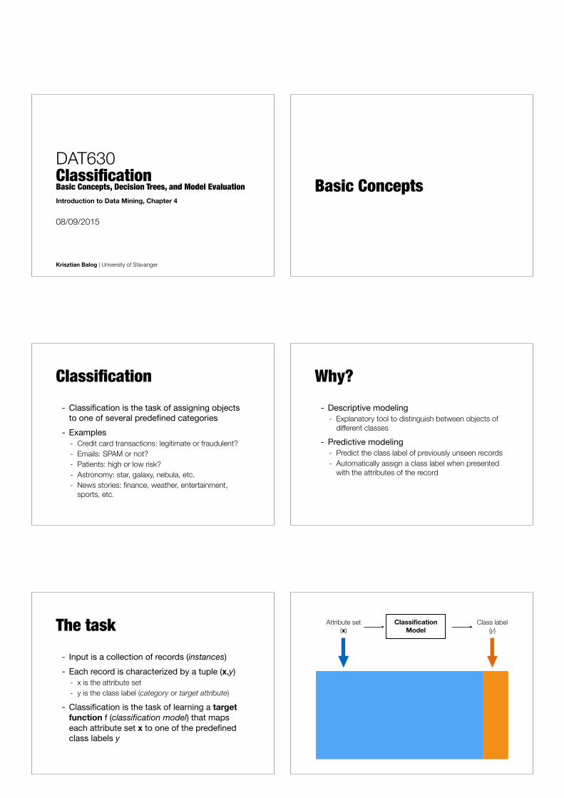
The task- Input is a collection of records (instances)- Each record is characterized by a tuple (x,y)

- x is the attribute set - y is the class label (category or target attribute)

- Classification is the task of learning a target function f (classification model) that maps each attribute set x to one of the predefined class labels y

Attribute set(x)

Class label(y)

Classification Model

Attribute set(x)

Class label(y)

Classification Model

NominalNominal

Ordinal

Interval

Ratio

General approach

Apply Model

Induction

Deduction

Learn Model

Model

Tid Attrib1 Attrib2 Attrib3 Class

1 Yes Large 125K No

2 No Medium 100K No

3 No Small 70K No

4 Yes Medium 120K No

5 No Large 95K Yes

6 No Medium 60K No

7 Yes Large 220K No

8 No Small 85K Yes

9 No Medium 75K No

10 No Small 90K Yes 10


11 No Small 55K ?

12 Yes Medium 80K ?

13 Yes Large 110K ?

14 No Small 95K ?

15 No Large 67K ? 10

Test Set

Learningalgorithm

Training Set

Records whose class labels are known

Records with unknown class labels

General approach

Apply Model

Induction

Deduction

Learn Model

Model


1 Yes Large 125K No

2 No Medium 100K No

3 No Small 70K No


5 No Large 95K Yes

6 No Medium 60K No

7 Yes Large 220K No

8 No Small 85K Yes

9 No Medium 75K No



11 No Small 55K ?

12 Yes Medium 80K ?

13 Yes Large 110K ?

14 No Small 95K ?


Test Set

Learningalgorithm

Training SetModel

Learning algorithm

Learn model

Apply model

Induction

Deduction

Objectives for Learning Alg.

Apply Model

Induction

Deduction

Learn Model

Model


1 Yes Large 125K No

2 No Medium 100K No

3 No Small 70K No


5 No Large 95K Yes

6 No Medium 60K No

7 Yes Large 220K No

8 No Small 85K Yes

9 No Medium 75K No



11 No Small 55K ?

12 Yes Medium 80K ?

13 Yes Large 110K ?

14 No Small 95K ?


Test Set

Learningalgorithm

Training SetModel

Learning algorithm

Learn model

Apply model

Induction

Deduction

Should fit the input data well

Should correctly predict class labels for unseen data

Learning Algorithms- Decision trees- Rule-based- Naive Bayes- Support Vector Machines- Random forests- k-nearest neighbors- …

Machine Learning vs. Data Mining

- Similar techniques, but different goal- Machine learning is focused on developing and

designing learning algorithms- More abstract, e.g., features are given

- Data Mining is applied Machine Learning- Performed by a person who has a goal in mind and

uses Machine Learning techniques on a specific dataset

- Much of the work is concerned with data (pre)processing and feature engineering

Today- Decision trees- Binary class labels

- Positive or Negative

Objectives for Learning Alg.

Apply Model

Induction

Deduction

Learn Model

Model


1 Yes Large 125K No

2 No Medium 100K No

3 No Small 70K No


5 No Large 95K Yes

6 No Medium 60K No

7 Yes Large 220K No

8 No Small 85K Yes

9 No Medium 75K No



11 No Small 55K ?

12 Yes Medium 80K ?

13 Yes Large 110K ?

14 No Small 95K ?


Test Set

Learningalgorithm

Training SetModel

Learning algorithm

Learn model

Apply model

Induction

Deduction

Should fit the input data well

Should correctly predict class labels for unseen data

How to measure this?

Evaluation- Measuring the performance of a classifier- Based on the number of records correctly and

incorrectly predicted by the model- Counts are tabulated in a table called the

confusion matrix - Compute various performance metrics based

on this matrix

Confusion Matrix

Predicted class

Positive Negative

Actual class

Positive True Positives (TP)

False Negatives (FN)

Negative False Positives (FP)

True Negatives (TN)

Confusion Matrix

Predicted class

Positive Negative

Actual class

Positive True Positives (TP)

False Negatives (FN)

Negative False Positives (FP)

True Negatives (TN)

Type I Errorraising a false alarm

Type II Errorfailing to raise an alarm

Example"Is the man innocent?"

Predicted class

Positive Innocent

Negative Guilty

Actual class

Positive Innocent

True Positive

Convicted

False Negative

Freed

Negative Guilty

False Positive

Convicted

True Negative

Freed

convicting an innocent person(miscarriage of justice)

letting a guilty person go free (error of impunity)

Evaluation Metrics- Summarizing performance in a single number- Accuracy

- Error rate

- We seek high accuracy, or equivalently, low error rate

Number of correct predictions

Total number of predictions

=

TP + TN

TP + FP + TN + FN

Number of wrong predictions

Total number of predictions

=

FP + FN

TP + FP + TN + FN

Exercise- Create confusion matrix- Compute Accuracy and Error rate

Decision Trees Motivational Example

How does it work?- Asking a series of questions about the

attributes of the test record- Each time we receive an answer, a follow-up

question is asked until we reach a conclusion about the class label of the record

Decision Tree Model

Apply Model

Induction

Deduction

Learn Model

Model


1 Yes Large 125K No

2 No Medium 100K No

3 No Small 70K No


5 No Large 95K Yes

6 No Medium 60K No

7 Yes Large 220K No

8 No Small 85K Yes

9 No Medium 75K No



11 No Small 55K ?

12 Yes Medium 80K ?

13 Yes Large 110K ?

14 No Small 95K ?


Test Set

Learningalgorithm

Training SetModel

Learning algorithm

Learn model

Apply model

Induction

Deduction

Decision Tree

Decision Tree Root nodeno incoming edgeszero or more outgoing edges

Decision Tree

Internal nodeexactly one incoming edges two or more outgoing edges

Decision Tree

Leaf (or terminal) nodeshave exactly one incoming edgesand no outgoing edges

Example Decision Tree

Tid Refund MaritalStatus

TaxableIncome Cheat

1 Yes Single 125K No

2 No Married 100K No

3 No Single 70K No

4 Yes Married 120K No

5 No Divorced 95K Yes

6 No Married 60K No

7 Yes Divorced 220K No

8 No Single 85K Yes

9 No Married 75K No

10 No Single 90K Yes10

categorical

categorical

continuous

class

Refund

MarSt

TaxInc

YES NO

NO

NO

Yes No

Married Single, Divorced

< 80K > 80K

Splitting Attributes

Training Data Model: Decision Tree

Another Example


TaxableIncome Cheat



3 No Single 70K No



6 No Married 60K No


8 No Single 85K Yes

9 No Married 75K No


categorical

categorical

continuous

class MarSt

Refund

TaxInc

YES NO

NO

NO

Yes No

Married Single,

Divorced

< 80K > 80K

There could be more than one tree that fits the same data!

Apply Model to Test Data

Apply Model

Induction

Deduction

Learn Model

Model


1 Yes Large 125K No

2 No Medium 100K No

3 No Small 70K No


5 No Large 95K Yes

6 No Medium 60K No

7 Yes Large 220K No

8 No Small 85K Yes

9 No Medium 75K No



11 No Small 55K ?

12 Yes Medium 80K ?

13 Yes Large 110K ?

14 No Small 95K ?


Test Set

Learningalgorithm

Training SetModel

Learning algorithm

Learn model

Apply model

Induction

Deduction

Refund

MarSt

TaxInc

YESNO

NO

NO

Yes No


< 80K > 80K

Refund Marital Status

Taxable Income Cheat

No Married 80K ? 10

Test DataStart from the root of tree.

Refund

MarSt

TaxInc

YESNO

NO

NO

Yes No


< 80K > 80K



No Married 80K ? 10

Test Data

Refund

MarSt

TaxInc

YESNO

NO

NO

Yes No


< 80K > 80K



No Married 80K ? 10

Test Data

Refund

MarSt

TaxInc

YESNO

NO

NO

Yes No


< 80K > 80K



No Married 80K ? 10

Test Data

Refund

MarSt

TaxInc

YESNO

NO

NO

Yes No


< 80K > 80K



No Married 80K ? 10

Test Data

Refund

MarSt

TaxInc

YESNO

NO

NO

Yes No


< 80K > 80K



No Married 80K ? 10

Test Data

Assign Cheat to “No”

Decision Tree Induction

Apply Model

Induction

Deduction

Learn Model

Model


1 Yes Large 125K No

2 No Medium 100K No

3 No Small 70K No


5 No Large 95K Yes

6 No Medium 60K No

7 Yes Large 220K No

8 No Small 85K Yes

9 No Medium 75K No



11 No Small 55K ?

12 Yes Medium 80K ?

13 Yes Large 110K ?

14 No Small 95K ?


Test Set

Learningalgorithm

Training SetModel

Learning algorithm

Learn model

Apply model

Induction

Deduction

Tree Induction- There are exponentially many decision trees

that can be constructed from a given set of attributes

- Finding the optimal tree is computationally infeasible (NP-hard)

- Greedy strategies are used - Grow a decision tree by making a series of locally

optimum decisions about which attribute to use for splitting the data

Hunt’s algorithm- Let Dt be the set of training records that

reach a node t and y={y1,…yc} the class labels

- General Procedure- If Dt contains records that belong the

same class yt, then t is a leaf node labeled as yt

- If Dt is an empty set, then t is a leaf node labeled by the default class, yd

- If Dt contains records that belong to more than one class, use an attribute test to split the data into smaller subsets. Recursively apply the procedure to each subset.

Tid Refund Marital Status




3 No Single 70K No



6 No Married 60K No


8 No Single 85K Yes

9 No Married 75K No

10 No Single 90K Yes 10

Dt

?

Don’t Cheat

Refund

Don’t Cheat

Don’t Cheat

Yes No

Refund

Don’t Cheat

Yes No

Marital Status

Don’t Cheat

Cheat

Single, Divorced Married

Taxable Income

Don’t Cheat

< 80K >= 80K

Refund

Don’t Cheat

Yes No

Marital Status

Don’t Cheat

Cheat

Single, Divorced Married


TaxableIncome Cheat



3 No Single 70K No



6 No Married 60K No


8 No Single 85K Yes

9 No Married 75K No


Tree Induction Issues- Determine how to split the records

- How to specify the attribute test condition? - How to determine the best split?

- Determine when to stop splitting




How to Specify Test Condition?• Depends on attribute types

- Nominal - Ordinal - Continuous

• Depends on number of ways to split- 2-way split - Multi-way split

Splitting Based on Nominal Attributes• Multi-way split: Use as many partitions as

distinct values.

• Binary split: Divides values into two subsets. Need to find optimal partitioning.

CarTypeFamily

SportsLuxury

CarType{Family, Luxury} {Sports}

CarType{Sports, Luxury} {Family} OR

Splitting Based on Ordinal Attributes• Multi-way split: Use as many partitions as

distinct values.

• Binary split: Divides values into two subsets. Need to find optimal partitioning.

SizeSmall

MediumLarge

Size{Medium,

Large} {Small}Size

{Small, Medium} {Large}

OR

Splitting Based on Continuous Attributes

- Different ways of handling- Discretization to form an ordinal categorical attribute

- Static – discretize once at the beginning - Dynamic – ranges can be found by equal interval bucketing,

equal frequency bucketing (percentiles), or clustering

- Binary Decision: (A < v) or (A ≥ v)- consider all possible splits and finds the best cut - can be more compute intensive

Splitting Based on Continuous Attributes

TaxableIncome> 80K?

Yes No

TaxableIncome?

(i) Binary split (ii) Multi-way split

< 10K

[10K,25K) [25K,50K) [50K,80K)

> 80K




Determining the Best Split

OwnCar?

C0: 6C1: 4

C0: 4C1: 6

C0: 1C1: 3

C0: 8C1: 0

C0: 1C1: 7

CarType?

C0: 1C1: 0

C0: 1C1: 0

C0: 0C1: 1

StudentID?

...

Yes No Family

Sports

Luxury c1 c10

c20

C0: 0C1: 1

...

c11

Before Splitting: 10 records of class 0, 10 records of class 1

Which test condition is the best?

Determining the Best Split• Greedy approach:

- Nodes with homogeneous class distribution are preferred

• Need a measure of node impurity:

C0: 5C1: 5

C0: 9C1: 1

Non-homogeneous, High degree of impurity

Homogeneous, Low degree of impurity

Impurity Measures- Measuring the impurity of a node

- P(i|t) = fraction of records belonging to class i at a given node t

- c is the number of classes

Entropy(t) = �c�1X

i=0

P (i|t)log2P (i|t)

Classification error(t) = 1�maxP (i|t)

Gini(t) = 1�c�1X

i=0

P (i|t)2

Entropy

•Maximum (log nc) when records are equally distributed among all classes implying least information •Minimum (0.0) when all records belong to one

class, implying most information

Entropy(t) = �c�1X

i=0

P (i|t)log2P (i|t)

Exercise Entropy(t) = �c�1X

i=0

P (i|t)log2P (i|t)

C1 0 C2 6

C1 2 C2 4

C1 1 C2 5

Exercise Entropy(t) = �c�1X

i=0

P (i|t)log2P (i|t)

C1 0 C2 6

C1 2 C2 4

C1 1 C2 5

P(C1) = 0/6 = 0 P(C2) = 6/6 = 1 Entropy = – 0 log 0 – 1 log 1 = – 0 – 0 = 0

P(C1) = 1/6 P(C2) = 5/6 Entropy = – (1/6) log2 (1/6) – (5/6) log2 (1/6) = 0.65

P(C1) = 2/6 P(C2) = 4/6 Entropy = – (2/6) log2 (2/6) – (4/6) log2 (4/6) = 0.92

GINI

- Maximum (1 - 1/nc) when records are equally distributed among all classes, implying least interesting information

- Minimum (0.0) when all records belong to one class, implying most interesting information


i=0

P (i|t)2

Exercise

C1 0 C2 6

C1 2 C2 4

C1 1 C2 5


i=0

P (i|t)2

Exercise

C1 0 C2 6

C1 2 C2 4

C1 1 C2 5

P(C1) = 0/6 = 0 P(C2) = 6/6 = 1 Gini = 1 – P(C1)2 – P(C2)2 = 1 – 0 – 1 = 0

P(C1) = 1/6 P(C2) = 5/6 Gini = 1 – (1/6)2 – (5/6)2 = 0.278

P(C1) = 2/6 P(C2) = 4/6 Gini = 1 – (2/6)2 – (4/6)2 = 0.444


i=0

P (i|t)2 Classification Error

• Maximum (1 - 1/nc) when records are equally distributed among all classes, implying least interesting information

• Minimum (0.0) when all records belong to one class, implying most interesting information

Classification error(t) = 1�maxP (i|t)

Exercise Classification error(t) = 1�maxP (i|t)

C1 0 C2 6

C1 2 C2 4

C1 1 C2 5

Exercise Classification error(t) = 1�maxP (i|t)

C1 0 C2 6

C1 2 C2 4

C1 1 C2 5

P(C1) = 0/6 = 0 P(C2) = 6/6 = 1 Error = 1 – max (0, 1) = 1 – 1 = 0

P(C1) = 1/6 P(C2) = 5/6 Error = 1 – max (1/6, 5/6) = 1 – 5/6 = 1/6

P(C1) = 2/6 P(C2) = 4/6 Error = 1 – max (2/6, 4/6) = 1 – 4/6 = 1/3

Comparison of Impurity MeasuresFor a 2-class problem:

Gain = goodness of a split

B?

Yes No

Node N3 Node N4

A?

Yes No

Node N1 Node N2

Before Splitting:

C0 N10 C1 N11

C0 N20 C1 N21

C0 N30 C1 N31

C0 N40 C1 N41

C0 N00 C1 N01

M0

M1 M2 M3 M4

M12 M34Gain = M0 – M12 vs M0 – M34

Information Gain- When Entropy is used as the impurity measure,

it’s called information gain- Measures how much we gain by splitting a

parent nodenumber of attribute values

total number of records at the parent node

number of records associated with the

child node vj

�

info

= Entropy(p)�kX

j=1

N(vj

)

NEntropy(v

j

)

Determining the Best Split

OwnCar?

C0: 6C1: 4

C0: 4C1: 6

C0: 1C1: 3

C0: 8C1: 0

C0: 1C1: 7

CarType?

C0: 1C1: 0

C0: 1C1: 0

C0: 0C1: 1

StudentID?

...

Yes No Family

Sports

Luxury c1 c10

c20

C0: 0C1: 1

...

c11

Before Splitting: 10 records of class 0, 10 records of class 1

Which test condition is the best?

Gain Ratio

- It the attribute produces a large number of splits, its split info will also be large, which in turn reduces its gain ratio

Gain ratio =

�

info

Split info

Split info = �kX

i=1

P (vi) log2 P (vi)




Stopping Criteria for Tree Induction• Stop expanding a node when all the records

belong to the same class• Stop expanding a node when all the records

have similar attribute values• Early termination

Summary Decision Trees- Inexpensive to construct- Extremely fast at classifying unknown records- Easy to interpret for small-sized trees- Accuracy is comparable to other classification

techniques for many simple data sets

Practical Issues of Classification

Underfitting and Overfitting500 circular and 500 triangular data points.

Circular points: 0.5 ≤ sqrt(x1

2+x22) ≤ 1

Triangular points: sqrt(x1

2+x22) > 0.5 or

sqrt(x12+x2

2) < 1

Underfitting and OverfittingOverfitting

Underfitting: when model is too simple, both training and test errors are large

How to Address Overfitting• Pre-Pruning (Early Stopping Rule)

- Stop the algorithm before it becomes a fully-grown tree - Typical stopping conditions for a node: • Stop if all instances belong to the same class • Stop if all the attribute values are the same

- More restrictive conditions: • Stop if number of instances is less than some user-

specified threshold • Stop if class distribution of instances are independent

of the available features

• Stop if expanding the current node does not improve impurity measures (e.g., Gini or information gain)

How to Address Overfitting…• Post-pruning

- Grow decision tree to its entirety - Trim the nodes of the decision tree in a bottom-up fashion - If generalization error improves after trimming, replace sub-

tree by a leaf node - Class label of leaf node is determined from majority class of

instances in the sub-tree

Methods for estimating performance

- Holdout- Reserve 2/3 for training and 1/3 for testing

(validation set)

- Cross validation- Partition data into k disjoint subsets - k-fold: train on k-1 partitions, test on the remaining

one - Leave-one-out: k=n

Expressivity

y < 0.33?

: 0 : 3

: 4 : 0

y < 0.47?

: 4 : 0

: 0 : 4

x < 0.43?

Yes

Yes

No

No Yes No

0 0.1 0.2 0.3 0.4 0.5 0.6 0.7 0.8 0.9 10

0.1

0.2

0.3

0.4

0.5

0.6

0.7

0.8

0.9

1

x

y

Expressivity

x + y < 1

Class = + Class =

Use-case: Web Robot Detection

Assignment 1

Tasks- Given a training data set and a test set- Task 1: Build a decision tree classifier

- You have to build it from scratch - You are free to pick your programming language - Submit code and predicted class labels for test set - Accuracy has to reach a certain threshold

Tasks- Task 2: Submit a short report describing

- What processing steps you applied - Which are the most important features of the dataset

(based on the decision tree built)

- Task 3 (optional) Use any classifier from a the scikit-learn Python machine learning library- Submit code and predicted class labels for test set

Online evaluation- Real-time leaderboard will be available for the

submissions (updated after each git push)- Two tracks, results separately

- Decision tree track (for everyone) - Open track (optional)

- Best teams for each track get +5 points at the exam (all members)

- Online evaluation be available from next week

Practicalities- Data set and specific instructions will be made

available today- Work in groups of 2-3- Deadlines

- Forming groups by 11/9 (this Friday!) - Predictions due 28/9 - Report due 5/10

- Note: I’m away this Friday, but the practicum will be held. Get started on Assignment 1!

20150908-lecture-3-draft asd def hfl dfgf lkreglker lerg kelr gk

Documents