A Beginner’s Course in Boundary Element Methods

Whye-Teong Ang

Universal Publishers Boca Raton, Florida

A Beginner’s Course in Boundary Element Methods

Copyright © 2007 Whye-Teong Ang All rights reserved.

Universal Publishers Boca Raton, Florida • USA

2007

ISBN: 1-58112-974-2 13-ISBN: 978-1-58112-974-8

www.universal-publishers.com

Preface

During the last few decades, the boundary element method,also known as the boundary integral equation method or bound-ary integral method, has gradually evolved to become one ofthe few widely used numerical techniques for solving bound-ary value problems in engineering and physical sciences. Inimplementing the method, only the boundary of the solutiondomain has to be discretized into elements. In the case of atwo-dimensional problem, this is really easy to do. Put closelypacked points on the boundary (a curve) and join up two con-secutive neighboring points to form straight line elements.

In March 1985, when I started research work for a doctoraldegree in the Department of Applied Mathematics at the Uni-versity of Adelaide, Australia, I was introduced to the methodby my thesis supervisor, David L Clements. At that time, theterm “boundary element method” was relatively new. It wasapparently first used in a 1977 paper by CA Brebbia and JDominguez1. Carlos Brebbia and his co-researchers had un-doubtedly played an important role in introducing the methodto the engineering research community. Apparently less than200 journal papers whose titles contained the term “boundaryelement method” could be found in 1985. In 2006, there wereseveral thousand or perhaps even more such papers.

The history of the method could, however, be traced backto an earlier time, well before the 1970s. The mathematicsthat laid the theoretical foundation for the development of themethod could be found in the works of famous mathemati-cians like Laplace, Gauss, Green, Fredholm, Betti, Somigliana,Muskhelishvili, Mikhlin and Kupradze. In the 1960s, there wereattempts at using electronic computers to approximate solu-tions of potential problems through the use of boundary inte-gral equations, notably the pioneering works of MA Jaswon and

1CA Brebbia and J Dominguez, “Boundary element methods for po-tential problems,” Applied Mathematical Modelling, Volume 1, 1977, pp.372-378.

i

GT Symm2. The work of Frank J Rizzo3 was regarded by manyresearchers as the beginning of a novel direct boundary integralmethod for the numerical solution of elasticity problems.

After completing my doctoral work in the middle of 1987,I continued to keep myself informed on the development ofthe boundary integral method and related mathematical works,pick up some new ideas now and then, attend conferences, givetalks and seminars, and contribute to boundary element re-search with applications to problems in engineering and phys-ical sciences. Some specific research areas I had worked onusing the boundary integral method include linear fracture me-chanics (accurate computation of stress intensity factors usingspecial Green’s functions), analyses of nonhomogeneous media(such as functionally graded materials), diffusion with speci-fication of mass, modeling of photonic crystal fibers, integralformulation of imperfect interfaces and bioheat transfer.

Sometimes, I undertook the task of introducing the methodto beginners, mainly advanced undergraduate and research stu-dents who were working on projects under my supervision. Todo this, I had produced various notes over a period of time.The chapters in this book were written based on those notes.In writing this book, I assume that the readers have some priorbasic knowledge of vector calculus (covering topics such as line,surface and volume integrals and the various integral theorems),ordinary and partial differential equations, complex variablesand computer programming.

FORTRAN 77 codes for the numerical procedures discussedare listed in the chapters4. Some justifications, if any is needed

2One may refer to the following papers: (a) MA Jaswon, “An integralequation method in potential theory I,” Proceedings of the Royal Societyof London Series A, Volume 275, 1963, pp. 23-32, and (b) GT Symm, “Anintegral equation method in potential theory II,” Proceedings of the RoyalSociety of London Series A, Volume 275, 1963, pp. 33-46.

3FJ Rizzo, “An integral equation approach to boundary value problemsof classical elastostatics,” Quarterly of Applied Mathematics, Volume 25,1967, pp. 83-95. This was the work presented by FJ Rizzo in his doctoraldissertation. Much later on in 1993, it won him an ASME Warner Medal.

4Readers who are interested in obtaining the codes in electronic formmay e-mail me at mwtang@ntu.edu.sg.

ii

at all, for using good old FORTRAN 77 would be as follows.Firstly, in spite of its seniority, it still remains a powerful “num-ber crunching tool”. Secondly, its codes are relatively easyto decipher and would be of some use even to readers whoare attempting to implement the numerical procedures usingnewer software tools (such as C++ and MATLAB). Thirdly,free FORTRAN 77 compilers (e.g. FTN77 from Salford Soft-ware and GNU Fortran) can be downloaded from the internet.

The constant encouragement and support of my dear wife,Young-Soon, had greatly motivated me to start and finish writ-ing this book. I would like to thank Ean-Hin Ooi, Lukito Jaya-putra, Bao Ing Yun, Jackson R Jones, Joris Vankerschaver andAlessandro Vaccari for informing me of errors in an earlier ver-sion of this book and Jeff Young and Rebekah Galy of UniversalPublishers for their prompt replies to all my questions on thepublication of this book.

Whye-Teong Ang, Singapore, 2007, 2014

iii

Contents

1 Two-dimensional Laplace’s Equation 71.1 Introduction . . . . . . . . . . . . . . . . . . . . . 71.2 Fundamental Solution . . . . . . . . . . . . . . . 91.3 Reciprocal Relation . . . . . . . . . . . . . . . . . 111.4 Boundary Integral Solution . . . . . . . . . . . . 121.5 Boundary Element Solution with Constant Ele-

ments . . . . . . . . . . . . . . . . . . . . . . . . 191.6 Formulae for Integrals of Constant Elements . . . 221.7 Implementation on Computer . . . . . . . . . . . 261.8 Numerical Examples . . . . . . . . . . . . . . . . 371.9 Summary and Discussion . . . . . . . . . . . . . 481.10 Exercises . . . . . . . . . . . . . . . . . . . . . . 50

2 Discontinuous Linear Elements 542.1 Introduction . . . . . . . . . . . . . . . . . . . . . 542.2 Boundary Element Solution with Discontinuous

Linear Elements . . . . . . . . . . . . . . . . . . 562.3 Formulae for Integrals of Discontinuous Linear

Elements . . . . . . . . . . . . . . . . . . . . . . 612.4 Implementation on Computer . . . . . . . . . . . 642.5 Numerical Examples . . . . . . . . . . . . . . . . 692.6 Summary and Discussion . . . . . . . . . . . . . 772.7 Exercises . . . . . . . . . . . . . . . . . . . . . . 78

3 Two-dimensional Helmholtz Type Equation 813.1 Introduction . . . . . . . . . . . . . . . . . . . . . 813.2 Homogeneous Helmholtz Equation . . . . . . . . 83

iv

3.2.1 Fundamental Solution . . . . . . . . . . . 833.2.2 Boundary Integral Solution . . . . . . . . 853.2.3 Numerical Procedure . . . . . . . . . . . . 853.2.4 Implementation on Computer . . . . . . . 88

3.3 Helmholtz Type Equation with Variable Coeffi-cients . . . . . . . . . . . . . . . . . . . . . . . . 993.3.1 Integral Formulation . . . . . . . . . . . . 993.3.2 Approximation of Domain Integral . . . . 1033.3.3 Dual-reciprocity Boundary Element Pro-

cedure . . . . . . . . . . . . . . . . . . . . 1063.3.4 Implementation on Computer . . . . . . . 109

3.4 Summary and Discussion . . . . . . . . . . . . . 1203.5 Exercises . . . . . . . . . . . . . . . . . . . . . . 122

4 Two-dimensional Diffusion Equation 1254.1 Introduction . . . . . . . . . . . . . . . . . . . . . 1254.2 Solution by Dual-reciprocity Boundary Element

Method . . . . . . . . . . . . . . . . . . . . . . . 1274.3 Time-stepping Approach . . . . . . . . . . . . . . 1334.4 Implementation on Computer . . . . . . . . . . . 1374.5 Numerical Examples . . . . . . . . . . . . . . . . 1444.6 Summary and Discussion . . . . . . . . . . . . . 1524.7 Exercises . . . . . . . . . . . . . . . . . . . . . . 153

5 Green’s Functions for Potential Problems 1565.1 Introduction . . . . . . . . . . . . . . . . . . . . . 1565.2 Half Plane . . . . . . . . . . . . . . . . . . . . . . 157

5.2.1 Two Special Green’s Functions . . . . . . 1575.2.2 Applications . . . . . . . . . . . . . . . . 160

5.3 Infinitely Long Strip . . . . . . . . . . . . . . . . 1785.3.1 Derivation of Green’s Functions by Con-

formal Mapping . . . . . . . . . . . . . . 1785.3.2 Applications . . . . . . . . . . . . . . . . 183

5.4 Exterior Region of a Circle . . . . . . . . . . . . 1885.4.1 Two Special Green’s Functions . . . . . . 1885.4.2 Applications . . . . . . . . . . . . . . . . 191

5.5 Summary and Discussion . . . . . . . . . . . . . 1955.6 Exercises . . . . . . . . . . . . . . . . . . . . . . 195

v

6 Three-dimensional Problems 1986.1 Introduction . . . . . . . . . . . . . . . . . . . . . 1986.2 Laplace’s Equation . . . . . . . . . . . . . . . . . 198

6.2.1 Boundary Value Problem . . . . . . . . . 1986.2.2 Fundamental Solution . . . . . . . . . . . 1996.2.3 Reciprocal Relation . . . . . . . . . . . . 2006.2.4 Boundary Integral Equation . . . . . . . . 2006.2.5 Boundary Element Method . . . . . . . . 2036.2.6 Computation of Integrals over Surface El-

ements . . . . . . . . . . . . . . . . . . . . 2056.2.7 Implementation on Computer . . . . . . . 209

6.3 Homogeneous Helmholtz Equation . . . . . . . . 2256.4 Helmholtz Type Equation with Variable Coeffi-

cients . . . . . . . . . . . . . . . . . . . . . . . . 2326.4.1 Dual-reciprocity Boundary Element Pro-

cedure . . . . . . . . . . . . . . . . . . . . 2326.4.2 Implementation on Computer . . . . . . . 235

6.5 Summary and Discussion . . . . . . . . . . . . . 2456.6 Exercises . . . . . . . . . . . . . . . . . . . . . . 246

vi

Chapter 1

Two-dimensionalLaplace’s Equation

1.1 Introduction

Perhaps a good starting point for introducing boundary ele-ment methods is through solving boundary value problems gov-erned by the two-dimensional Laplace’s equation

∂2φ

∂x2+

∂2φ

∂y2= 0. (1.1)

The Laplace’s equation occurs in the formulation of prob-lems in many diverse fields of studies in engineering and physi-cal sciences, such as thermostatics, elastostatics, electrostatics,magnetostatics, ideal fluid flow and flow in porous media.

An interior boundary value problem which is of practicalinterest requires solving Eq. (1.1) in the two-dimensional regionR (on the Oxy plane) bounded by a simple closed curve Csubject to the boundary conditions

φ = f1(x, y) for (x, y) ∈ C1,∂φ

∂n= f2(x, y) for (x, y) ∈ C2, (1.2)

where f1 and f2 are suitably prescribed functions and C1 andC2 are non-intersecting curves such that C1 ∪ C2 = C. Referto Figure 1.1 for a geometrical sketch of the problem.

7

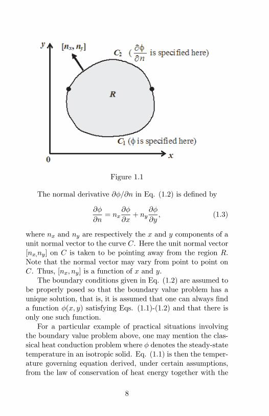
Figure 1.1

The normal derivative ∂φ/∂n in Eq. (1.2) is defined by

∂φ

∂n= nx

∂φ

∂x+ ny

∂φ

∂y, (1.3)

where nx and ny are respectively the x and y components of aunit normal vector to the curve C. Here the unit normal vector[nx,ny] on C is taken to be pointing away from the region R.Note that the normal vector may vary from point to point onC. Thus, [nx, ny] is a function of x and y.

The boundary conditions given in Eq. (1.2) are assumed tobe properly posed so that the boundary value problem has aunique solution, that is, it is assumed that one can always finda function φ(x, y) satisfying Eqs. (1.1)-(1.2) and that there isonly one such function.

For a particular example of practical situations involvingthe boundary value problem above, one may mention the clas-sical heat conduction problem where φ denotes the steady-statetemperature in an isotropic solid. Eq. (1.1) is then the temper-ature governing equation derived, under certain assumptions,from the law of conservation of heat energy together with the

8

Fourier’s heat flux model. The heat flux out of the region Racross the boundary C is given by −κ∂φ/∂n, where κ is thethermal heat conductivity of the solid. Thus, the boundaryconditions in Eq. (1.2) imply that at each and every givenpoint on C either the temperature or the heat flux (but notboth) is known. To determine the temperature field in thesolid, one has to solve Eq. (1.1) in R to find the solution thatsatisfies the prescribed boundary conditions on C.

In general, it is difficult (if not impossible) to solve exactlythe boundary value problem defined by Eqs. (1.1)-(1.2). Themathematical complexity involved depends on the geometricalshape of the region R and the boundary conditions given in Eq.(1.2). Exact solutions can only be found for relatively simplegeometries of R (such as a square region) together with partic-ular boundary conditions. For more complicated geometries orgeneral boundary conditions, one may have to resort to numer-ical (approximate) techniques for solving Eqs. (1.1)-(1.2).

This chapter introduces a boundary element method for thenumerical solution of the interior boundary value problem de-fined by Eqs. (1.1)-(1.2). We show how a boundary integral so-lution can be derived for Eq. (1.1) and applied to obtain a sim-ple boundary element procedure for approximately solving theboundary value problem under consideration. The implemen-tation of the numerical procedure on the computer, achievedthrough coding in FORTRAN 77, is discussed in detail.

1.2 Fundamental Solution

If we use polar coordinates r and θ centered about (0, 0), asdefined by x = r cos θ and y = r sin θ, and introduce ψ(r, θ) =φ(r cos θ, r sin θ), we can rewrite Eq. (1.1) as

1

r

∂

∂r(r∂ψ

∂r) +

1

r2∂2ψ

∂θ2= 0. (1.4)

For the case in which ψ is independent of θ, that is, if ψis a function of r alone, Eq. (1.4) reduces to the ordinary

9

differential equation

d

dr(rd

dr[ψ(r)]) = 0 for r 6= 0. (1.5)

The ordinary differential equation in Eq. (1.5) can be easilyintegrated twice to yield the general solution

ψ(r) = A ln(r) +B, (1.6)

where A and B are arbitrary constants.From (1.6), it is obvious that the two-dimensional Laplace’s

equation in Eq. (1.1) admits a class of particular solutions givenby

φ(x, y) = A lnpx2 + y2 +B for (x, y) 6= (0, 0). (1.7)

If we choose the constants A and B in (1.7) to be 1/(2π)and 0 respectively and shift the center of the polar coordinatesfrom (0, 0) to the general point (ξ, η), a particular solution ofEq. (1.1) is

φ(x, y) =1

2πlnp(x− ξ)2 + (y − η)2 for (x, y) 6= (ξ, η).

(1.8)

As we shall see, the particular solution in Eq. (1.8) plays animportant role in the development of boundary element meth-ods for the numerical solution of the interior boundary valueproblem defined by Eqs. (1.1)-(1.2). We specially denote thisparticular solution using the symbol Φ(x, y; ξ, η), that is, wewrite

Φ(x, y; ξ, η) =1

4πln[(x− ξ)2 + (y − η)2]. (1.9)

We refer to Φ(x, y; ξ, η) in Eq. (1.9) as the fundamentalsolution of the two-dimensional Laplace’s equation. Note thatΦ(x, y; ξ, η) satisfies Eq. (1.1) everywhere except at (ξ, η) whereit is not well defined.

10

1.3 Reciprocal Relation

If φ1 and φ2 are any two solutions of Eq. (1.1) in the regionR bounded by the simple closed curve C then it can be shownthat Z

C

(φ2∂φ1∂n− φ1

∂φ2∂n

)ds(x, y) = 0. (1.10)

Eq. (1.10) provides a reciprocal relation between any twosolutions of the Laplace’s equation in the region R bounded bythe curve C. It may be derived from the two-dimensional versionof the Gauss-Ostrogradskii (divergence) theorem as explainedbelow.

According to the divergence theorem, if F= u(x, y)i+v(x, y)jis a well defined vector function such that∇·F= ∂u/∂x+∂v/∂yexists in the region R bounded by the simple closed curve Cthen Z

C

F · n ds(x, y) =ZZR

∇ · F dxdy,

that is,ZC

[unx + vny]ds(x, y) =

ZZR

[∂u

∂x+

∂v

∂y]dxdy,

where n = [nx, ny] is the unit normal vector to the curve C,pointing away from the region R.

Since φ1 and φ2 are solutions of Eq. (1.1), we may write

∂2φ1∂x2

+∂2φ1∂y2

= 0,

∂2φ2∂x2

+∂2φ2∂y2

= 0.

If we multiply the first equation by φ2 and the second oneby φ1 and take the difference of the resulting equations, we

11

obtain

∂

∂x(φ2

∂φ1∂x− φ1

∂φ2∂x) +

∂

∂y(φ2

∂φ1∂y− φ1

∂φ2∂y) = 0,

which can be integrated over R to giveZZR

[∂

∂x(φ2

∂φ1∂x− φ1

∂φ2∂x) +

∂

∂y(φ2

∂φ1∂y− φ1

∂φ2∂y)]dxdy = 0.

Application of the divergence theorem to convert the doubleintegral over R into a line integral over C yieldsZC

[(φ2∂φ1∂x− φ1

∂φ2∂x)nx + (φ2

∂φ1∂y− φ1

∂φ2∂y)ny]ds(x, y) = 0

which is essentially Eq. (1.10).Together with the fundamental solution given by Eq. (1.9),

the reciprocal relation in Eq. (1.10) can be used to derivea useful boundary integral solution for the two-dimensionalLaplace’s equation.

1.4 Boundary Integral Solution

Let us take φ1 = Φ(x, y; ξ, η) (the fundamental solution as de-fined in Eq. (1.9)) and φ2 = φ, where φ is the required solutionof the interior boundary value problem defined by Eqs. (1.1)-(1.2).

Since Φ(x, y; ξ, η) is not well defined at the point (ξ, η), thereciprocal relation in Eq. (1.10) is valid for φ1 = Φ(x, y; ξ, η)and φ2 = φ only if (ξ, η) does not lie in the region R∪C. Thus,Z

C

[φ(x, y)∂

∂n(Φ(x, y; ξ, η))

−Φ(x, y; ξ, η) ∂∂n(φ(x, y))]ds(x, y)

= 0 for (ξ, η) /∈ R ∪ C. (1.11)

12

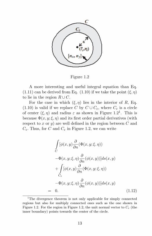
Figure 1.2

A more interesting and useful integral equation than Eq.(1.11) can be derived from Eq. (1.10) if we take the point (ξ, η)to lie in the region R ∪ C.

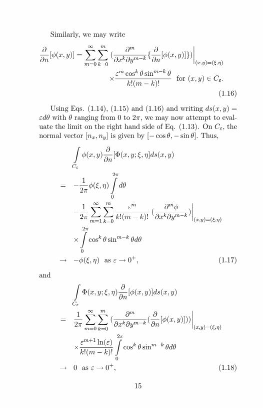
For the case in which (ξ, η) lies in the interior of R, Eq.(1.10) is valid if we replace C by C ∪ Cε, where Cε is a circleof center (ξ, η) and radius ε as shown in Figure 1.21. This isbecause Φ(x, y; ξ, η) and its first order partial derivatives (withrespect to x or y) are well defined in the region between C andCε. Thus, for C and Cε in Figure 1.2, we can write

ZC

[φ(x, y)∂

∂n(Φ(x, y; ξ, η))

−Φ(x, y; ξ, η) ∂∂n(φ(x, y))]ds(x, y)

+

ZCε

[φ(x, y)∂

∂n(Φ(x, y; ξ, η))

−Φ(x, y; ξ, η) ∂∂n(φ(x, y))]ds(x, y)

= 0. (1.12)

1The divergence theorem is not only applicable for simply connectedregions but also for multiply connected ones such as the one shown inFigure 1.2. For the region in Figure 1.2, the unit normal vector to Cε (theinner boundary) points towards the center of the circle.

13

Eq. (1.12) holds for any radius ε > 0, so long as the circleCε (in Figure 1.2) lies completely inside the region bounded byC. Thus, we may let ε→ 0+ in Eq. (1.12). This givesZ

C

[φ(x, y)∂

∂n(Φ(x, y; ξ, η))

−Φ(x, y; ξ, η) ∂∂n(φ(x, y))]ds(x, y)

= − limε→0+

ZCε

[φ(x, y)∂

∂n(Φ(x, y; ξ, η))

−Φ(x, y; ξ, η) ∂∂n(φ(x, y))]ds(x, y). (1.13)

Using polar coordinates r and θ centered about (ξ, η) asdefined by x− ξ = r cos θ and y − η = r sin θ, we may write

Φ(x, y; ξ, η) =1

2πln(r),

∂

∂n[Φ(x, y; ξ, η)] = nx

∂

∂x[Φ(x, y; ξ, η)] + ny

∂

∂y[Φ(x, y; ξ, η)]

=nx cos θ + ny sin θ

2πr. (1.14)

The Taylor’s series of φ(x, y) about the point (ξ, η) is givenby

φ(x, y) =∞Xm=0

mXk=0

(∂mφ

∂xk∂ym−k)

¯̄̄̄(x,y)=(ξ,η)

(x− ξ)k(y − η)m−k

k!(m− k)! .

On the circle Cε, r = ε. Thus,

φ(x, y) =∞Xm=0

mXk=0

(∂m

∂xk∂ym−k[φ(x, y)])

¯̄̄̄(x,y)=(ξ,η)

×εm cosk θ sinm−k θk!(m− k)! for (x, y) ∈ Cε. (1.15)

14

Similarly, we may write

∂

∂n[φ(x, y)] =

∞Xm=0

mXk=0

(∂m

∂xk∂ym−k{ ∂

∂n[φ(x, y)]})

¯̄̄̄(x,y)=(ξ,η)

×εm cosk θ sinm−k θk!(m− k)! for (x, y) ∈ Cε.

(1.16)

Using Eqs. (1.14), (1.15) and (1.16) and writing ds(x, y) =εdθ with θ ranging from 0 to 2π, we may now attempt to eval-uate the limit on the right hand side of Eq. (1.13). On Cε, thenormal vector [nx, ny] is given by [− cos θ,− sin θ]. Thus,Z

Cε

φ(x, y)∂

∂n[Φ(x, y; ξ, η]ds(x, y)

= − 12π

φ(ξ, η)

2πZ0

dθ

− 12π

∞Xm=1

mXk=0

εm

k!(m− k)! (∂mφ

∂xk∂ym−k)

¯̄̄̄(x,y)=(ξ,η)

×2πZ0

cosk θ sinm−k θdθ

→ −φ(ξ, η) as ε→ 0+, (1.17)

and ZCε

Φ(x, y; ξ, η)∂

∂n[φ(x, y)]ds(x, y)

=1

2π

∞Xm=0

mXk=0

(∂m

∂xk∂ym−k(∂

∂n[φ(x, y)]))

¯̄̄̄(x,y)=(ξ,η)

× εm+1 ln(ε)

k!(m− k)!

2πZ0

cosk θ sinm−k θdθ

→ 0 as ε→ 0+, (1.18)

15

since εm+1 ln(ε)→ 0 as ε→ 0+ for m = 0, 1, 2, · · · .Consequently, as ε→ 0+, Eq. (1.13) yields

φ(ξ, η) =

ZC

[φ(x, y)∂

∂n(Φ(x, y; ξ, η))

−Φ(x, y; ξ, η) ∂∂n(φ(x, y))]ds(x, y)

for (ξ, η) ∈ R. (1.19)

Together with Eq. (1.9), Eq. (1.19) provides us with aboundary integral solution for the two-dimensional Laplace’sequation. If both φ and ∂φ/∂n are known at all points onC, the line integral in Eq. (1.19) can be evaluated (at leastin theory) to calculate φ at any point (ξ, η) in the interior ofR. From the boundary conditions (1.2), however, at any givenpoint on C, either φ or ∂φ/∂n, not both, is known.

To solve the interior boundary value problem, we must findthe unknown φ and ∂φ/∂n on C2 and C1 respectively. As weshall see later on, this may be done through manipulation ofdata on the boundary C only, if we can derive a boundaryintegral formula for φ(ξ, η), similar to the one in Eq. (1.19), fora general point (ξ, η) that lies on C.

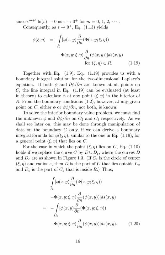
For the case in which the point (ξ, η) lies on C, Eq. (1.10)holds if we replace the curve C by D∪Dε, where the curves Dand Dε are as shown in Figure 1.3. (If Cε is the circle of center(ξ, η) and radius ε, then D is the part of C that lies outside Cε

and Dε is the part of Cε that is inside R.) Thus,ZD

[φ(x, y)∂

∂n(Φ(x, y; ξ, η))

−Φ(x, y; ξ, η) ∂∂n(φ(x, y))]ds(x, y)

= −ZDε

[φ(x, y)∂

∂n(Φ(x, y; ξ, η))

−Φ(x, y; ξ, η) ∂∂n(φ(x, y))]ds(x, y). (1.20)

16

Let us examine what happens to Eq. (1.20) when we letε→ 0+.

As ε→ 0+, the curve D tends to C. Thus, we may writeZC

[φ(x, y)∂

∂n(Φ(x, y; ξ, η))

−Φ(x, y; ξ, η) ∂∂n(φ(x, y))]ds(x, y)

= − limε→0+

ZDε

[φ(x, y)∂

∂n(Φ(x, y; ξ, η))

−Φ(x, y; ξ, η) ∂∂n(φ(x, y))]ds(x, y). (1.21)

Figure 1.3

Note that, unlike in Eq. (1.13), the line integral over C inEq. (1.21) is improper as its integrand is not well defined at(ξ, η) which lies on C. Strictly speaking, the line integrationshould be over the curve C without an infinitesimal segmentthat contains the point (ξ, η), that is, the line integral over Cin Eq. (1.21) has to be interpreted in the Cauchy principalsense if (ξ, η) lies on C.

To evaluate the limit on the right hand side of Eq. (1.21),we need to know what happens to Dε when we let ε→ 0+. Now

17

if (ξ, η) lies on a smooth part of C (not at where the gradientof the curve changes abruptly, that is, not at a corner point, ifthere is any), one can intuitively see that the part of C inside Cε

approaches an infinitesimal straight line as ε → 0+. Thus, weexpect Dε to tend to a semi-circle as ε→ 0+, if (ξ, η) lies on asmooth part of C. It follows that in attempting to evaluate thelimit on the right hand side of Eq. (1.21) we have to integrateover only half a circle (instead of a full circle as in the case ofEq. (1.13)).

Modifying Eqs. (1.17) and (1.18), we obtain

limε→0+

ZDε

φ(x, y)∂

∂n[Φ(x, y; ξ, η)]ds(x, y) = −1

2φ(ξ, η),

limε→0+

ZDε

Φ(x, y; ξ, η)∂

∂n[φ(x, y)]ds(x, y) = 0.

Hence Eq. (1.21) gives

1

2φ(ξ, η) =

ZC

[φ(x, y)∂

∂n(Φ(x, y; ξ, η))

−Φ(x, y; ξ, η) ∂∂n(φ(x, y))]ds(x, y)

for (ξ, η) lying on a smooth part of C.

(1.22)

Together with the boundary conditions in Eq. (1.2), Eq.(1.22) may be applied to obtain a numerical procedure for de-termining the unknown φ and/or ∂φ/∂n on the boundary C.Once φ and ∂φ/∂n are known at all points on C, the solutionof the interior boundary value problem defined by Eqs. (1.1)-(1.2) is given by Eq. (1.19) at any point (ξ, η) inside R. Moredetails are given in Section 1.5 below.

For convenience, we may write Eqs. (1.11), (1.19) and(1.22) as a single equation given by

18

λ(ξ, η)φ(ξ, η) =

ZC

[φ(x, y)∂

∂n(Φ(x, y; ξ, η))

−Φ(x, y; ξ, η) ∂∂n(φ(x, y))]ds(x, y),

(1.23)

if we define

λ(ξ, η) =

0 if (ξ, η) /∈ R ∪ C,1/2 if (ξ, η) lies on a smooth part of C,1 if (ξ, η) ∈ R.

(1.24)

1.5 Boundary Element Solution with Con-stant Elements

We now show how Eq. (1.23) may be applied to obtain a simpleboundary element procedure for solving numerically the interiorboundary value problem defined by Eqs. (1.1)-(1.2).

The boundary C is discretized into N very small straightline segments C(1), C(2), · · · , C(N−1) and C(N), that is,

C ' C(1) ∪ C(2) ∪ · · · ∪ C(N−1) ∪ C(N). (1.25)

The sides or the boundary elements C(1), C(2), · · · , C(N−1)and C(N) are constructed as follows. We put N well spacedout points given by (x(1), y(1)), (x(2), y(2)), · · · , (x(N−1), y(N−1))and (x(N), y(N)) on C, in the order given, following the counterclockwise direction. Defining (x(N+1), y(N+1)) = (x(1), y(1)),we take C(k) to be the boundary element from (x(k), y(k)) to(x(k+1), y(k+1)) for k = 1, 2, · · · , N.

As an example, in Figure 1.4, the boundary C = C1∪C2 inFigure 1.1 is approximated using 5 boundary elements denotedby C(1), C(2), C(3), C(4) and C(5).

19

Figure 1.4

For a simple approximation of φ and ∂φ/∂n on the bound-ary C, we assume that these functions are constants over eachof the boundary elements. Specifically, we make the approxi-mation:

φ ' φ(k)

and∂φ

∂n= p(k) for (x, y) ∈ C(k) (k = 1, 2, · · · , N),

(1.26)

where φ(k)and p(k) are respectively the values of φ and ∂φ/∂n

at the midpoint of C(k).With Eqs. (1.25) and (1.26), we find that Eq. (1.23) can

be approximately written as

λ(ξ, η)φ(ξ, η) =NXk=1

{φ(k)F (k)2 (ξ, η)− p(k)F (k)1 (ξ, η)}, (1.27)

where

F (k)1 (ξ, η) =

ZC(k)

Φ(x, y; ξ, η)ds(x, y),

F (k)2 (ξ, η) =

ZC(k)

∂

∂n[Φ(x, y; ξ, η)]ds(x, y). (1.28)

20

For a given k, either φ(k)or p(k) (not both) is known from

the boundary conditions in Eq. (1.2). Thus, there are N un-known constants on the right hand side of Eq. (1.27). To deter-mine their values, we have to generate N equations containingthe unknowns.

If we let (ξ, η) in Eq. (1.27) be given in turn by the mid-points of C(1), C(2), · · · , C(N−1) and C(N), we obtain1

2φ(m)

=NXk=1

{φ(k)F (k)2 (x(m), y(m))− p(k)F (k)1 (x(m), y(m))}

for m = 1, 2, · · · ,N, (1.29)

where (x(m), y(m)) is the midpoint of C(m).In the derivation of Eq. (1.29), we take λ(x(m), y(m)) = 1/2,

since (x(m), y(m)) being the midpoint of C(m) lies on a smoothpart of the approximate boundary C(1) ∪C(2) ∪ · · ·∪C(N−1) ∪C(N).

Eq. (1.29) constitutes a system of N linear algebraic equa-tions containing the N unknowns on the right hand side of Eq.(1.27). We may rewrite it as

NXk=1

a(mk)z(k) =NXk=1

b(mk) for m = 1, 2, · · · , N, (1.30)

where a(mk), b(mk) and z(k) are defined by

a(mk) =

−F (k)1 (x(m), y(m)) if φ is specified over C(k),

F (k)2 (x(m), y(m))− 12δ(mk) if ∂φ/∂n is

specified over C(k),

b(mk) =

φ(k)(−F (k)2 (x(m), y(m)) + 1

2δ(mk))

if φ is specified over C(k),

p(k)F (k)1 (x(m), y(m)) if ∂φ/∂n is specified

over C(k),

δ(mk) =

½0 if m 6= k,1 if m = k,

z(k) =

(p(k) if φ is specified over C(k),

φ(k)if ∂φ/∂n is specified over C(k).

(1.31)

21

Note that z(1), z(2), · · · , z(N−1) and z(N) are theN unknownconstants on the right hand side of Eq. (1.27), while a(mk) andb(mk) are known coefficients.

Once Eq. (1.30) is solved for the unknowns z(1), z(2), · · · ,z(N−1) and z(N), the values of φ and ∂φ/∂n over the element

C(k), as given by φ(k)and p(k) respectively, are known for k = 1,

2, · · · , N. Eq. (1.27) with λ(ξ, η) = 1 then provides us with anexplicit formula for computing φ in the interior of R, that is,

φ(ξ, η) 'NXk=1

{φ(k)F (k)2 (ξ, η)− p(k)F (k)1 (ξ, η)} for (ξ, η) ∈ R.

(1.32)

To summarize, a boundary element solution of the interiorboundary value problem defined by Eqs. (1.1)-(1.2) is givenby Eq. (1.32) together with Eqs. (1.28), (1.30) and (1.31).Because of the approximation in Eqs. (1.25) and (1.26), thesolution is said to be obtained using constant elements. Ana-

lytical formulae for calculating F (k)1 (ξ, η) and F (k)2 (ξ, η) in Eq.(1.28) are given in Eqs. (1.37), (1.38), (1.40) and (1.41) (to-gether with Eq. (1.35)) in the section below.

1.6 Formulae for Integrals of Constant El-ements

The boundary element solution above requires the evaluation of

F (k)1 (ξ, η) and F (k)2 (ξ, η). These functions are defined in termsof line integrals over C(k) as given in Eq. (1.28). The lineintegrals can be worked out analytically as follows.

Points on the element C(k) may be described using the para-metric equations

x = x(k) − t`(k)n(k)yy = y(k) + t`(k)n

(k)x

)from t = 0 to t = 1, (1.33)

where `(k) is the length of C(k) and [n(k)x , n

(k)y ] = [y(k+1) −

y(k), x(k)−x(k+1)]/`(k) is the unit normal vector to C(k) pointingaway from R.

22

For (x, y) ∈ C(k), we find that ds(x, y) =p(dx)2 + (dy)2 =`(k)dt and

(x− ξ)2 + (y − η)2 = A(k)t2 +B(k)(ξ, η)t+E(k)(ξ, η), (1.34)

where

A(k) = [`(k)]2,

B(k)(ξ, η) = [−n(k)y (x(k) − ξ) + (y(k) − η)n(k)x ](2`(k)),

E(k)(ξ, η) = (x(k) − ξ)2 + (y(k) − η)2. (1.35)

For any point (ξ, η), the parameters in Eq. (1.35) satisfy4A(k)E(k)(ξ, η) − [B(k)(ξ, η)]2 ≥ 0. To see why this is true,consider the straight line defined by the parametric equations

x = x(k) − t`(k)n(k)y and y = y(k) + t`(k)n(k)x for −∞ < t < ∞.

Note that C(k) is a subset of this straight line (given by theparametric equations from t = 0 to t = 1). Eq. (1.34) alsoholds for any point (x, y) lying on the extended line. If (ξ, η)does not lie on the line then A(k)t2+B(k)(ξ, η)t+E(k)(ξ, η) > 0for all real values of t (that is, for all points (x, y) on the line)and hence 4A(k)E(k)(ξ, η) − [B(k)(ξ, η)]2 > 0. On the otherhand, if (ξ, η) is on the line, we can find exactly one point(x, y) such that A(k)t2 + B(k)(ξ, η)t + E(k)(ξ, η) = 0. As eachpoint (x, y) on the line is given by a unique value of t, we con-clude that 4A(k)E(k)(ξ, η)− [B(k)(ξ, η)]2 = 0 for (ξ, η) lying onthe line.

From Eqs. (1.28), (1.33) and (1.34), F (k)1 (ξ, η) and F (k)2 (ξ, η)may be written as

F (k)1 (ξ, η) =`(k)

4π

1Z0

ln[A(k)t2 +B(k)(ξ, η)t+E(k)(ξ, η)]dt,

F (k)2 (ξ, η) =`(k)

2π

1Z0

n(k)x (x(k) − ξ) + n

(k)y (y(k) − η)

A(k)t2 +B(k)(ξ, η)t+E(k)(ξ, η)dt.

(1.36)

The second integral in Eq. (1.36) is the easiest one to workout for the case in which 4A(k)E(k)(ξ, η)− [B(k)(ξ, η)]2 = 0. For

23