DUST DISPERSION MODELING FOR OPENCAST MINES

A THESIS SUBMITTED IN PARTIAL FULFILLMENT OF

THE REQUIREMENTS

FOR THE DEGREE OF

BACHELOR OF TECHNOLOGY IN

MINING ENGINEERING

BY

JINESH VORA

DEPARTMENT OF MINING ENGINEERING NATIONAL INSTITUTE OF TECHNOLOGY

ROURKELA – 769 008 2010

DUST DISPERSION MODELING FOR OPENCAST MINES

A THESIS SUBMITTED IN PARTIAL FULFILLMENT OF THE REQUIREMENTS

FOR THE DEGREE OF

BACHELOR OF TECHNOLOGY IN

MINING ENGINEERING

BY

JINESH VORA

UNDER THE GUIDANCE OF

Dr. H. B. SAHU

Associate Professor

DEPARTMENT OF MINING ENGINEERING NATIONAL INSTITUTE OF TECHNOLOGY

ROURKELA – 769 008 2010

I

NATIONAL INSTITUTE OF TECHNOLOGY

ROURKELA

C E R T I F I C A T E

This is to certify that the thesis entitled ―Dust Dispersion Modeling for Opencast Mines‖

submitted by Mr Jinesh Vora in partial fulfillment of the requirements for the award of

Bachelor of Technology degree in Mining Engineering at the National Institute of

Technology, Rourkela; is an authentic work carried out by him under my supervision and

guidance.

To the best of my knowledge, the matter embodied in the thesis has not been submitted to

any other University/Institute for the award of any Degree or Diploma.

DATE: Dr H. B. Sahu

Associate Professor

Dept. of Mining Engineering

National Institute of Technology

Rourkela, 769008

II

ACKNOWLEDGEMENT

I record my sincere gratitude to Dr. H. B. Sahu, Associate Professor, Department of Mining

Engineering for introducing the present topic and for his inspiring guidance, constructive

criticism and valuable suggestion throughout this project work.

I would like to thank the officials of state pollution control board for providing me the necessary

data for this present work.

I would also like to convey my sincere gratitude to the faculty and staff members of Department

of Mining Engineering, NIT Rourkela, for their help at different times.

I would also like to extend my sincere thanks to Er. Rajesh Kanungo, Managing Director, Sun

Consultancy and Services, Bhubaneswar for his help in understanding the finer points of air

quality modeling and guidance in learning the AERMOD software

Last but not the least; I would like to thank my friends who have been a constant source of help

to me.

Jinesh Vora

Roll. No. - 10605032

III

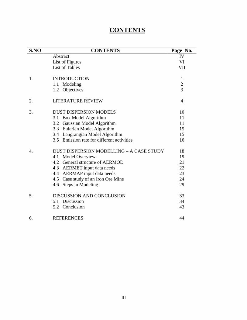
CONTENTS

S.NO CONTENTS Page No. Abstract IV

List of Figures VI

List of Tables VII

1. INTRODUCTION 1

1.1 Modeling 2

1.2 Objectives 3

2. LITERATURE REVIEW 4

3. DUST DISPERSION MODELS 10

3.1 Box Model Algorithm 11

3.2 Gaussian Model Algorithm 11

3.3 Eulerian Model Algorithm 15

3.4 Langrangian Model Algorithm 15

3.5 Emission rate for different activities 16

4. DUST DISPERSION MODELLING – A CASE STUDY 18

4.1 Model Overview 19

4.2 General structure of AERMOD 21

4.3 AERMET input data needs 22

4.4 AERMAP input data needs 23

4.5 Case study of an Iron Ore Mine 24

4.6 Steps in Modeling 29

5. DISCUSSION AND CONCLUSION 33

5.1 Discussion 34

5.2 Conclusion 43

6. REFERENCES 44

IV

ABSTRACT

INTRODUCTION

Mining operations generates substantial quantities of airborne respirable dust, which leads to the

development of lung disease in mine workers. Coal worker's pneumoconiosis and silicosis are lung

diseases that have adversely impacted the health of thousands of mine workers. The increasing trend of

opencast mining leads to release of huge amount of dust. These air borne dust particles, generally below

100 micron in size, are environmentally nuisance and cause health hazards as an ill effect of mining

activities. Opencast extraction activities like drilling, blasting, material handling and transport are a

potential source of air pollution. Therefore, a detailed study on emission sources and quantification of

pollutant concentration by means of dispersion modeling is required to access the environmental impact

of a opencast mine. On the basis of the predicted increments to air pollutant concentrations, an effective

mitigation and environmental plan can be devised for sensitive areas.

EXPERIMENTAL MATERIALS AND METHODS

In the present study an iron ore mine in West Singhbhum district of Jharkhand was selected. Air quality

modeling software named AERMOD (Version 6.2.1) was used. Meteorological data for the period

October 2008 – December 2008 was collected. 12 ambient air quality stations were set up for the purpose

of monitoring. Mining Data for Line source Modeling and Volume Source Modeling (Production, No.of

trips/hr, road width, road length etc.) was collected from the Mine.

Line source modeling and volume source modeling was carried out using AERMOD and isopleths for

dust for both line source and volume source were generated.

DISCUSSION Meteorological data was processed in RAMMET and windrose diagram for the area has been generated

and it was observed that the Pre-dominant wind direction is from North with 25.63 % calm condition and

the wind speed is 2.04 m /sec. Windrose showing Stability class is also generated Stability Class was

found to be F. Assessed Suspended Particle Levels (SPM) due to fugitive dust levels at nearby villages is

given in Table 1 and it was found that the resultant SPM level at these locations will remain within the

NAAQS norms. Isopleths for fugitive dusts (Line Source) and isopleths for fugitive dusts (Volume

Source) are generated which are presented in figure 1 and figure 2 respectively.

Table 1 Fugitive Dust Contribution at nearby locations

Location

ID

Direction

from

Mines

Distance

from

Mines

(Km)

Fugitive Dust (in g/m3)

NAAQS

(g/m3)

Background

Conc.

Incremental Conc. (Contribution

due to proposed Mines) Resultant

Conc. Volume

Source

Modeling

Line

Source

Modeling

Total

Incremental

Conc.

AAQ1 -- 0 178.0 0.00204 0.55811 0.56015 178.5602 500

AAQ2 -- 0 173.4 0.00293 0.10460 0.10753 173.5075 500

AAQ3 -- 0 164.3 0.00009 0.12878 0.12887 164.4289 500

AAQ4 SSE 2.8 159.7 0.00018 0.05489 0.05507 159.7551 200

AAQ5 SSW 2.6 152.7 0.00002 0.04730 0.04732 152.7473 200

V

AAQ6 N 2.0 156.3 0.00007 0.01101 0.01108 156.3111 200

AAQ7 NE 2.5 146.2 0.00001 0.00236 0.00237 146.2024 200

AAQ8 NW 3.5 157.4 0.00110 0.05941 0.06051 157.4605 200

AAQ9 NW 1.8 154.3 0.00002 0.00222 0.00224 154.3022 200

AAQ10 NE 2.5 151.7 0.00017 0.01324 0.01341 151.7134 200

AAQ11 N 3.3 156.3 0.00000 0.00195 0.00195 156.302 200

AAQ12 N 2.0 145.3 0.00013 0.01176 0.01189 145.3119 200

CONCLUSION

Air quality modeling has been attempted using AERMOD. Line source & Volume source modeling has

been carried out for haul road and open pit respectively. Wind rose and stability class diagram for the

area for the monitoring period has been generated. From the modeling exercise, dust concentrations at

certain receptor locations have been predicted and it was found that the resultant SPM level at these

locations will remain within the NAAQS norms. With use of meteorological data, dust concentration data

and emission data, isopleths for mining area could be generated using AERMOD. AERMOD could be

used not only for existing mines but for also proposed mines. It can predict dust concentrations and

accordingly measures for dust control could be adopted.

REFERENCES

Chaulya, S.K., ―Air Quality status of an Open Pit Mining Area in India‖, Environment Monitoring and

Assessment (2005) 105: Page no. 369 – 389

Reed, W.R., ―Significant Dust Dispersion Models for Mining Operations‖, Information Circular 9478,

2005, DHHS (NIOSH) Publication No. 2005 –138

Figure 1: Isopleths for fugitive dusts (Line source

Modeling

Figure 2: Isopleths for fugitive dusts (Volume

source Modeling

VI

LIST OF FIGURES

Figure No. Title of the Figure Page No.

3.1 Schematic representation of Gaussian Plume 12

3.2 Plume Rise 13

3.3 Plume Shapes 14

4.1 Dataflow in AERMOD Modeling System 20

4.2 Ambient air quality locations 25

4.3 Windrose Diagram 29

4.4 Stability Class Diagram 30

4.5 Wind class frequency Distribution 30

4.6 Isopleths of Fugitive Dust (Line Source

Modeling)

31

4.7 Isopleths of Fugitive Dust (Volume Source

Modeling)

32

5.1 Windrose diagram 34

5.2 Stability Class 35

VII

LIST OF TABLES

Table No. Title of the table Page No.

2.3 Emission rate for different activities 16

4.1 Micro-meteorological Data 26

4.2 Mining Data for Line Source modeling 27

4.3 Mining Data for Volume Source modeling 28

5.1 Fugitive dust contribution at nearby locations 36

5.2 Incremental Concentration of Fugitive Dust (Volume

Source Modeling)

37 - 39

5.3 Incremental Concentration of Fugitive Dust (Line Source

Modeling)

40 - 42

1

CHAPTER 1

INTRODUCTION

2

1. INTRODUCTION

Historically and into the present day, mining operations have generated substantial quantities of

airborne respirable dust, which has led to the development of lung disease in mine workers. Coal

worker's pneumoconiosis and silicosis are lung diseases that have adversely impacted the health

of thousands of mine workers. Depending on the severity of the lung disease, symptoms range

from reduced breathing capacity to death. Although significant advances in dust control

technology have been realized, improved mining practices and equipment have meanwhile led to

record production levels which have in turn resulted in the generation of additional dust. One

tool that can be used to investigate dust generation and dispersion is computer modeling.

Dust of any kind when inhaled in large quantities lead to the development of respiratory

diseases such as pneumoconiosis, silicosis, siderosis etc. If silica is a component of respirable

dust, then the effects of exposure pose a very serious health concern. Silicosis has no cure and is

fatal. There are other adverse impacts from dust exposure in addition to health effects. It is

known that even small particle in air hinders visibility. Climate change may occur from 𝑃𝑀10

exposure because the small particles in the atmosphere absorb and reflect the radiation from the

sun, thus, affecting the cloud physics in atmosphere.

1.1 MODELING

Modeling or simulation is a process whereby a system is created to simulate a real-life situation.

Computer modeling is generally the most inexpensive and versatile method for analyzing a real-

life situation and has become prevalent for solving problems related to physical processes,

especially in research and development.

Simulation generally involves modeling a physical process and analyzing it through the

use of a personal computer. This analysis involves trial-and error methods applied to the model

and tested with the actual physical process to perfect the model. Once this process is completed,

the computer model can be used to identify problematic areas, and efforts can focus on finding

solutions to address these particular concerns. Computer modeling of dust dispersion from mine

sources can allow for the identification of potential hazard areas surrounding the source from a

health and safety standpoint. It can also allow for the evaluation of dust control techniques to

determine modifications necessary to improve dust control.

3

The results from modeling the emissions of a facility are used to ensure that the regional

air quality does not exceed the NAAQS or detiorate the air quality further. If the modeling

results show the facility will not cause the regional air quality to exceed the NAAQS or detiorate

the air quality then the air quality permit will be granted, otherwise the quality permit application

will be denied. Therefore, it is important that the modeling method accurately estimate both the

amount of pollutant a facility will emit and the pollutants dispersion.

Air quality modeling is used for determining and visualizing the significance and impact

of emissions to the atmosphere. Air quality models estimate the air pollutant concentration at

many locations which are referred to as receptors. These models provide a cost effective way to

analyze impacts over a wide spatial area where factors such as meteorology, topography and

emissions from nearby sources are considered. The source data is evaluated in conjunction with

meteorological information such as wind speed, wind direction, temperature etc. in the air quality

model. The model examines all of these components together to characterize the state of the

atmosphere and predict how pollutants are transported from the sources and estimates the

concentration of these pollutants in the atmosphere.

1.2 OBJECTIVES

The purpose of a dispersion model is to provide a means of calculating ambient ground-level

concentrations of an emitted substance given information about the emissions and the nature of

the atmosphere. The amount released can be determined from knowledge of the industrial

process or actual measurements. However, predictive compliance with an ambient air quality

objective is determined by the concentration of the substance at ground level. Air quality

objectives refer to concentration in the ambient air, not in the emission source. In order to assess

whether an emission meets the ambient air objective it is necessary to determine the ground-level

concentrations that may arise at various distances from the source. This is the function of a

dispersion model.

Therefore, the current work has been planned with the following objectives:

Selection of a mine for dust dispersion modeling

Collection of dust concentration data for various operations and at various locations.

Collection of micro-meteorological data for the duration of sampling.

Modeling of dust dispersion using the above data

4

CHAPTER 2

LITERATURE REVIEW

5

2. LITERATURE REVIEW

The dust dispersion models used in surface mining have been adopted from existing industrial air

pollution models. The surface models do not focus on particular size fraction and are applicable

to all size. Following is the summary of studies carried out by different researchers:

Cole and Fabrick (1984) have discussed pit retention of dust from surface mining operations.

They have suggested a very simplistic model that is representative of box – model algorithm and

is given as:

ε = 1

1+ 𝑉𝑑𝐾𝑧

𝐻

Where

ε = mass fraction of dust that escapes an open pit

𝑉𝑑 = particle deposition velocity (m/sec)

𝐾𝑧 = vertical diffusivity (𝑚2/ sec)

H = pit depth (m)

EPA (1995) Dust dispersion modeling for surface mining operations, as required for air quality

protection, was completed using an established model—the Industrial Source Complex model

(ISC3) created by EPA. This model also includes a subroutine for modeling flat/ complex terrain

and has the ability to model dispersion from four types of emissions sources: point, which are

typically stacks; volume, which are typically buildings; area, which are typically haul roads or

storage piles; and open pit. The ISC3 model is based on the Gaussian equation for point source

emissions which is given as:

χ = 𝑄𝐾𝑉𝐷

2𝜋𝑢𝑠𝜎𝑦𝜎𝑧 exp −0.5

𝑦

𝜎𝑦

2

Where,

Q = pollutant emission rate (g / sec)

K = scaling coefficient to convert calculated concentrations to desired units

V = vertical term

D = decay term

𝑢𝑠 = mean wind speed at release height (m/sec)

6

𝜎𝑦 , 𝜎𝑧 = standard deviation of lateral and vertical concentration distribution (m)

𝜒 = hourly concentration at downwind distance x (µg/𝑚3)

y = crosswind distance from source to receptor

Pereira et al. (1997) used a Gaussian dispersion equation to predict dust concentrations from the

stockpiles of an operating surface mine in Portugal. The equation is as follows:

c = 𝑄

2𝜋𝜎𝑦𝜎𝑧𝑢 exp −0.5

𝑦𝑟

𝜎𝑦

2

exp −0.5 𝑕𝑒 − 𝑧𝑟

𝜎𝑧

2

Where,

c = pollutant concentration at location receptor

Q = emission rate

𝜎𝑦 , 𝜎𝑧 = horizontal and vertical standard deviation respectively

ū = average wind speed

𝑕𝑒 = effective emission height

This equation was used to create risk maps of air quality for locations surrounding the mine site.

Ghose and Majee (2000) carried out assessment of dust generated due to opencast coal mines.

Emission factor data was used to quantify the generation of dust. The main sources of air

pollution were identified. It was estimated that due to topsoil removal, overburden (O/B)

removal, extraction of coal, size reduction generated 7.8 t of dust per day. Wind erosion

generated 1.6 t of dust per day and the whole operation produced dust which accounted for 9.4

t/day. This caused air pollution in the work zone and surrounding locations. This methodology

may be used to quantify generation for other projects also.

Reed et al. (2001) completed a study on the ISC3 model using a theoretical rock quarry. The

study also concluded that hauling operations contributed the majority of 𝑃𝑀10 concentrations

and that the haul truck emissions factors may be part of the cause of the overprediction of 𝑃𝑀10

concentrations by the ISC3 model. Reed described a model called the Dynamic Component

Program that can be used for predicting dust dispersion from haul trucks. The model is based on

a Gaussian equation similar to that used by the ISC3 model:

χ = 𝑄𝐾

2𝜋𝑤𝑠𝜎𝑦𝜎𝑧 exp −0.5

𝑦

𝜎𝑦

2

Where,

7

Q = pollutant emission rate (g/sec)

K = scaling coefficient to convert calculated concentrations to desired units

𝑤𝑠 = mean wind speed at release height (m/sec)

𝜎𝑦 , 𝜎𝑧 = standard deviation of lateral and vertical concentration distribution (m)

𝜒 = hourly concentration at downwind distance (µg/𝑚3)

y = crosswind distance from source to receptor (m)

The major difference between the Dynamic Component Program and the ISC3 model is the

methodology of applying the source emissions when predicting dust dispersion from that source.

Reed (2001) designed a computer model named the dynamic component program (DCP) for

predicting the dispersion of dust from haul trucks. Validation of DCP was completed by

comparing its results with the results of the ISC3 model and with actual dust measurements taken

from two operating mine sites. Comparisons of the field measurements, predictions of the ISC3

model and the prediction of DCP demonstrated that the results from the DCP represent, on

average an 85% improvement over the ISC3 dust dispersion model results. The DCP model

generally better predicts 𝑃𝑀10 dispersion from haul trucks by a factor of two to three. If the

frequency of haul trucks is high (over 200 trucks per day), then the DCP's performance becomes

significantly better. By comparing the modeling and field study results, it was concluded that the

following causes contributed to the overprediction of dust dispersion of the ISC3 model over the

actual results. The main reason was due to the inability of the ISC3 model to handle mobile

emissions sources.

Chaulya et al. (2003) carried out study for the determination of emission rate for SPM to

calculate emission rate of various opencast mining activities and validation of commonly used

two air quality models for Indian mining conditions. To achieve the objectives, eight coal and

three iron ore mining sites were selected to generate site specific emission data by considering

type of mining, method of working, geographical location, accessibility and above all resource

availability. The study covered various mining activities and locations including drilling,

overburden loading and unloading, coal/mineral loading and unloading, coal handling or

screening plant, exposed overburden dump, stock yard, workshop, exposed pit surface, transport

road and haul road. Validation of the study was carried out through Fugitive Dust Model (FDM)

and Point, Area and Line sources model (PAL2) by assigning the measured emission rate for

8

each mining activity, meteorological data and other details of the respective mine as an input to

the models. Both the models were run separately for the same set of input data for each mine to

get the predicted SPM concentration at three receptor locations for each mine. The receptor

locations were selected such a way that at the same places the actual filed measurement was

carried out for SPM concentration. Statistical analysis was carried out to assess the performance

of the models based on a set of measured and predicted SPM concentration data. The value of

coefficient of correlation for PAL2 and FDM was calculated to be 0.990–0.994 and 0.966–0.997,

respectively, which showed a fairly good agreement between measured and predicted values of

SPM concentration. The average index of agreement values for PAL2 and FDM was found to be

0.665 and 0.752, respectively, which showed that the prediction by PAL2 and FDM models are

accurate by 66.5 and 75.2%, respectively. These indicate that FDM model was more suited for

Indian mining conditions.

Singh et al (2006) carried out comparison and performance evaluation of dispersion models

FDM and ISCST3 for a gold mine at Goa. The emphasis of large-scale opencast mining had

resulted in widespread concern about the deterioration in environmental quality, specially the

increase in concentration of Suspended Particulate Matter (SPM) within and around the mining

site. Thus, to gain better understanding of the fate and transport of the pollutants and to predict

future conditions under various inputs and management action alternatives, the mathematical

simulation of the dispersion process was done. For this, application of the EPA models for the

short-term prediction of the pollution level due to mining activities was explored. The two

models considered in the study were Industrial Source Complex Short-Term (ISCST3) and

Fugitive Dust Model. The emission inventory and meteorological data were primary inputs for

air quality model. Various statistical approaches were used to compare and evaluate the models

under study and it was found that FDM is more accurate then ISCST3 and thus is more useful as

a screening tool for regulatory purposes.

Chakraborty et al. (2008) studied the dispersion of air borne dust generated due to mining

activities in Gughus opencast coal project, W.C.L. The concentration of gaseous pollutants such

as CO, 𝑁𝑂𝑥 etc. was much lower than the threshold limit values. Therefore the air quality

modleing was restricted to the determination of particulate matter i.e. SPM and RPM. Primary

data for analysis of air-borne dust dispersion included the activity wise generation of particulate

9

matters as well as micro-meteorological data. They used modified Pasquill and Gifford formula

for calculation of emission rate. Stability classes were found to be B, C & D. With the help of

mine plan, for locating different activities, activity wise emission rates and meteorological data,

Fugitive Dust Model was run and it was found that the ambient air quality at three sites of

Gughus OCP was well within the limits.

Trivedi et al. (2008) studied the different sources of dust generation due to coal mining activities

and quantification of dust emission and it’s dispersion for the Durgapur Opencast Coal Project of

Western Coalfields Limited. The dust dispersion in horizontal as well as vertical direction was

estimated by the procedure suggested by Pasquill and Gifford keeping in view the Pasquill

stability class of prevalent meteorological conditions. Dust emission rates for different point,

area and line sources were estimated considering the background dust concentration. Ambient air

quality data was generated for selected stations. And air quality modeling was attempted using

Fugitive Dust Model (FDM). With the help of FDM, dust concentration was predicted at the

source as well as at the selected receptors at different distances along downwind direction. The

air quality modeling using FDM revealed that the dust generated due to mining activities does

not contribute to ambient air quality significantly in surrounding areas beyond 500m in normal

meteorological conditions.

Trivedi et al. (2009) examined different sources of dust generation and quantified dust emission

rates from different point, area and line sources considering background dust concentration at

one of the opencast coal project of Western Coalfields limited. Air quality modeling using

Fugitive Dust Model revealed that dust generated due to mining activities did not contribute to

ambient air quality significantly in surrounding areas beyond 500 m in normal meteorological

conditions. Predicted values of total suspended particulate matter were 68 – 92 % of observed

values. They formulated a management strategy for effective control of air pollution at source

and other mitigative measures including green belt design were also recommended.

10

CHAPTER 3

DUST DISPERSION MODELS

11

3. DUST DISPERSION MODELS

Modeling of pollutant dispersion is completed using mathematical algorithms. There are several

basic mathematical algorithms in use

Box model

Gaussian model

Eulerian model

Lagrangian model

3.1 BOX MODEL ALGORITHM

The box model is the simplest of the modeling algorithms. It assumes the airshed in the shape of

a box. The box model is represented using following equation –

d(CV )

dt = Q*A + u*𝐶𝑖𝑛*W*H – u*C*W*H

Where,

Q = pollutant emission rate per unit area

C = homogeneous species concentration within the airshed

V = volume described by box

𝐶𝑖𝑛 = species concentration entering airshed

A = horizontal area of box

u = wind speed normal to the box

H = mixing height

Although useful, this model has limitations. It assumes the pollutant is homogeneous across the

airshed, and it is used to estimate average pollutant concentrations over very large area.

3.2 GAUSSIAN MODEL ALGORITHM

The Gaussian models are the most common mathematical models used for air dispersion. They

are based upon the assumption that the pollutant will disperse according to the normal statistical

distribution. Gaussian distribution equation is given by

C 𝑥, 𝑦, 𝑧 = 𝑄

2𝜋𝑢𝜎𝑦𝜎𝑧 exp

− 𝑧−𝑕 2

2𝜎𝑧2 + 𝑒𝑥𝑝

– 𝑧 + 𝑕 2

2𝜎𝑧2 exp

− 𝑦 2

2𝜎𝑦2

Where,

C 𝑥, 𝑦, 𝑧 = Pollutant concentration as a function of downwind position (x, y, z)

12

Q = mass emission rate

u = wind speed

𝜎𝑦= standard deviation of pollutant concentration in y (horizontal) direction

𝜎𝑧 = standard deviation of pollutant concentration in z (vertical) direction

y = distance in horizontal direction

z = distance in vertical direction

H = effective stack height

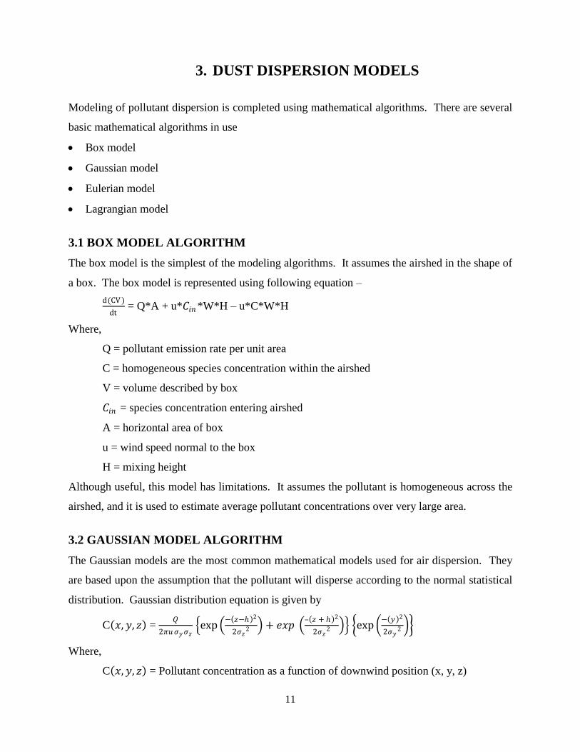
The Gaussian distribution determines the size of the plume downwind from the source. A

schematic representation of the Gaussian Plume is shown in Figure 3.1. The plume size is

dependent on the stability of the atmosphere and the dispersion of the plume in the horizontal

and vertical directions. These horizontal and vertical dispersion coefficients (σy and σz

respectively) are merely the standard deviation from normal on the Gaussian distribution curve

in the y and z directions. These dispersion coefficients, σy and σz, are functions of wind speed,

cloud cover, and surface heating by the sun. The Gaussian distribution requires that the material

in the plume be maintained.

Figure 3.1: Schematic Representation of Gaussian Plume

In order for a plume to be modeled using the Gaussian distribution the following assumption

must be made:

The plume spread has a normal distribution

13

The emission rate (Q) is constant and continuous

Wind speed and direction is uniform

Total reflection of the plume takes place at the surface

The terrain is relatively flat, i.e., no crosswind barriers

3.2.1 Plume Behaviour: The mixing of ambient air into the plume is called entrainment. As the

plume entrains air into it, the plume diameter grows as it travels downwind. A combination of

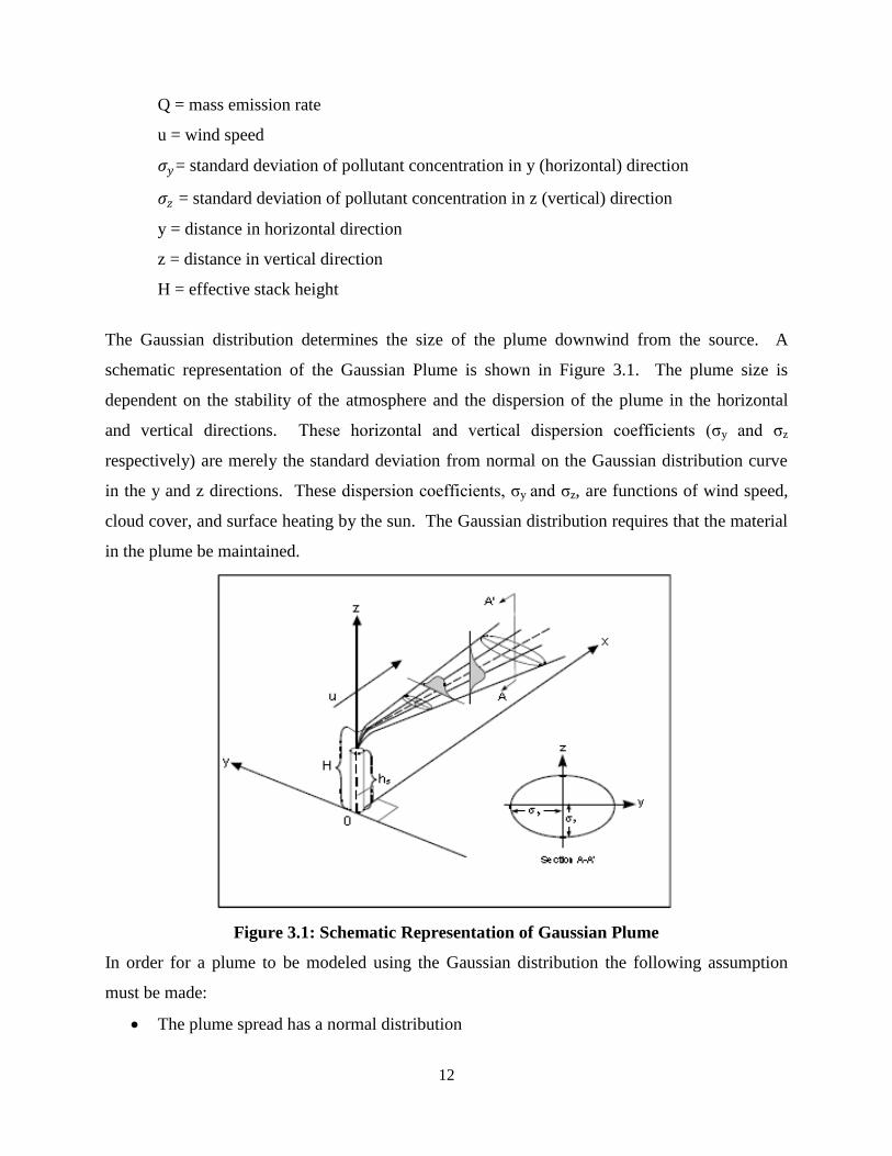
the gases' momentum and buoyancy causes the gases to rise. This is referred to as plume rise

and allows air pollutants emitted in this gas stream to be lofted higher in the atmosphere.

The final height of the plume, referred to as the effective stack height (H), is the sum of

the physical stack height (𝑕𝑠) and the plume rise (Δh). Plume rise is actually calculated as the

distance to the imaginary centerline of the plume rather than to the upper or lower edge of the

plume (Figure 3.2).

Figure 3.2: Plume Rise

The Briggs’ plume rise formula (1969) is as follows:

∆h = 1.6∗𝐹1/3∗𝑥2/3

ū

Where:

Δh = plume rise (above stack)

F = Buoyancy Flux (see below)

ū = average wind speed

14

x = downwind distance from the stack/

g = acceleration due to gravity (9.8 m/𝑠2)

V = volumetric flow rate of stack gas

𝑇𝑠 = temperature of stack gas

𝑇𝑎 = temperature of ambient air

Buoyancy flux = F = 𝑔

𝜋V(

𝑇𝑠−𝑇𝑎

𝑇𝑠)

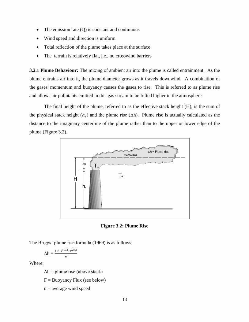
3.2.2 Plume Stability

Shapes of plumes depend upon atmospheric stability conditions which depend on Environmental

Lapse rate (ELR) and Dry Adiabatic Lapse Rate (DALR).

If,

ELR > DLR, atmosphere is stable

ELR >> DLR ,very stable atmosphere

ELR = DALR , atmosphere is neutral

ELR < DLR , atmosphere is unstable

Different plume shapes are presented in figure 3. 3

Figure 3.3: Plume Shapes

15

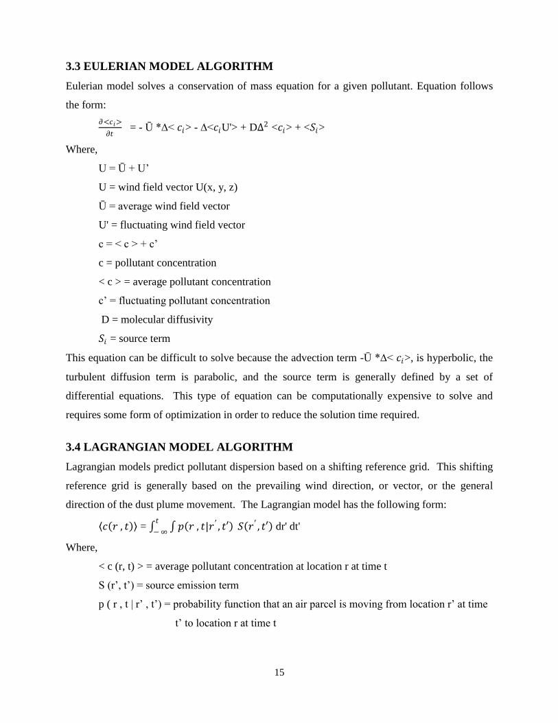
3.3 EULERIAN MODEL ALGORITHM

Eulerian model solves a conservation of mass equation for a given pollutant. Equation follows

the form:

𝜕<𝑐𝑖>

𝜕𝑡 = - Ū *∆< 𝑐𝑖> - ∆<𝑐𝑖U'> + D∆2 <𝑐𝑖> + <𝑆𝑖>

Where,

U = Ū + U’

U = wind field vector U(x, y, z)

Ū = average wind field vector

U' = fluctuating wind field vector

c = < c > + c’

c = pollutant concentration

< c > = average pollutant concentration

c’ = fluctuating pollutant concentration

D = molecular diffusivity

𝑆𝑖 = source term

This equation can be difficult to solve because the advection term -Ū *∆< 𝑐𝑖>, is hyperbolic, the

turbulent diffusion term is parabolic, and the source term is generally defined by a set of

differential equations. This type of equation can be computationally expensive to solve and

requires some form of optimization in order to reduce the solution time required.

3.4 LAGRANGIAN MODEL ALGORITHM

Lagrangian models predict pollutant dispersion based on a shifting reference grid. This shifting

reference grid is generally based on the prevailing wind direction, or vector, or the general

direction of the dust plume movement. The Lagrangian model has the following form:

𝑐 𝑟 , 𝑡 = 𝑝 𝑟 , 𝑡|𝑟′ , 𝑡′ 𝑡

− ∞𝑆 𝑟′ , 𝑡′ dr' dt'

Where,

< c (r, t) > = average pollutant concentration at location r at time t

S (r’, t’) = source emission term

p ( r , t | r’ , t’) = probability function that an air parcel is moving from location r’ at time

t’ to location r at time t

16

This mathematical model has limitations when its results are compared with actual

measurements. This is due to the dynamic nature of the model. Measurements are generally

made at stationary points, while the model predicts pollutant concentration based upon a moving

reference grid.

3.5 EMISSION RATE FOR DIFFERENT ACTIVITIES

Emission factor equations are required to relate the quantity of a pollutant released to the

atmosphere with an activity associated with the release of that pollutant. For calculation of

emission rate for different activities, Empirical equations by Chakraborty et al. (2002) are used

and these have been presented in Table 3.1

Table 3.1: Emission Rate for Different Activities

Activity Empirical Equation

Drilling: E = 0.0325 100 − 𝑚 𝑠𝑢 / 100 − 𝑠 𝑚 0.1 𝑑𝑓 0.3

Overburden loading: E = 0.018 100 − 𝑚 /𝑚 1.4 𝑠/ 100 − 𝑠 0.4

𝑢𝑕 ∗ 𝑙 0.1

Haul road: E = 100 − 𝑚 /𝑚 0.8 𝑠/ 100 − 𝑠 0.1

𝑢0.3 2663 +

0.1 𝑣 + 𝑓𝑐 10−6

Transport road: E = 100 − 𝑚 𝑠 / 100 − 𝑠 𝑚 0.1𝑢1.6 1.64 + 0.01 𝑣 + 𝑓 10−3

Overburden unloading: E = 1.76𝑕1/2 100 − 𝑚 /𝑚 0.2 𝑠/ 100 − 𝑠 2𝑢0.8 𝑐𝑦0.1

Mineral unloading: E = 0.023 100 − 𝑚 /𝑠𝑕 / 𝑚 100 − 𝑠 2𝑢3 𝑐𝑦0.1

Exposed O/B dump: E = 100 − 𝑚 /𝑚 0.2 𝑠/ 100 − 𝑠 0.1

𝑢/ 2.6 + 120𝑢 𝑎/ 0.2 + 276.5𝑎

Mineral handling plant: E = 100 − 𝑚 /𝑚 0.4 𝑎2𝑠/ 100 − 𝑠 0.3

𝑢/ 160 + 3.7𝑢

Exposed pit surface: E = 2.4 100 − 𝑚 /𝑚 0.8 𝑎𝑠/ 100 − 𝑠 0.1

𝑢/ 4 + 66𝑢 10−4

Overall Mine: E = 𝑢0.4𝑎0.2 9.7 + 0.01𝑝 + 𝑏/ 4 + 0.3𝑏

Parameters and units and symbols used in the above equations are:

m : Moisture content (%)

s : Silt content (%)

u : Wind speed (m/s)

d : Hole diameter (mm)

f : Frequency (no. of holes/day)

17

h : Drop height (m)

l : Size of loader (𝑚3)

v : Average vehicle speed (m/sec)

c : Capacity of dumper (ton)

a : area (𝑘𝑚2)

y : Frequency of unloading (no. / Hr)

x : Frequency of loading (no. / Hr)

p : Mineral production (Mt/yr)

b : OB handling (M𝑚3/yr)

E : Emission rate (g/sec)

18

CHAPTER 4

DUST DISPERSION MODELING

- A CASE STUDY

19

4. DUST DISPERSION MODELING – A CASE STUDY

In the present study an iron ore mine in West Singhbhum district of Jharkhand was selected. Air

quality modeling software named AERMOD (Version 6.2.1) was used. AERMOD is a steady-

state plume model that assumes that concentrations at all distances during a modeled hour are

governed by the temporally averaged meteorology of the hour. The steady state assumption

yields useful results since the statistics of the concentration distribution are of primary concern

rather than specific concentrations at particular times and locations. AERMOD has been

designed to handle the computation of pollutant impacts in both flat and complex terrain within

the same modeling framework.

4. 1 MODEL OVERVIEW

AERMOD was developed by the AERMIC (American Meteorological Society (AMS)/United

States Environmental Protection Agency (EPA) Regulatory Model Improvement Committee).

AERMOD model is applicable to rural and urban areas, flat and complex terrain, surface and

elevated releases, and multiple sources (including, point, area and volume sources). AERMOD

is a steady-state plume model. In the stable boundary layer (SBL), it assumes the concentration

distribution to be Gaussian in both the vertical and horizontal. In the convective boundary layer

(CBL), the horizontal distribution is also assumed to be Gaussian, but the vertical distribution is

described with a bi-Gaussian probability density function.

AERMOD constructs vertical profiles of required meteorological variables based on

measurements and extrapolations of those measurements using similarity (scaling) relationships.

Vertical profiles of wind speed, wind direction, turbulence, temperature, and temperature

gradient are estimated using all available meteorological observations. AERMOD requires only

a single surface measurement of wind speed, wind direction and ambient temperature. Like

ISC3, AERMOD also needs observed cloud cover.

The AERMOD atmospheric dispersion modeling system is an integrated system that

includes three modules:

A steady-state dispersion model designed for short dispersion of air pollutant emissions from

stationary industrial sources.

A meteorological data preprocessor (AERMET) that accepts surface meteorological data,

upper air soundings, and optionally, data from on-site instrument towers. It then calculates

20

atmospheric parameters needed by the dispersion model, such as atmospheric turbulence

characteristics, mixing heights, friction velocity, Monin-Obukov length and surface heat flux.

A terrain preprocessor (AERMAP) whose main purpose is to provide a physical relationship

between terrain features and the behavior of air pollution plumes. It generates location and

height data for each receptor location. It also provides information that allows the dispersion

model to simulate the effects of air flowing over hills or splitting to flow around hills

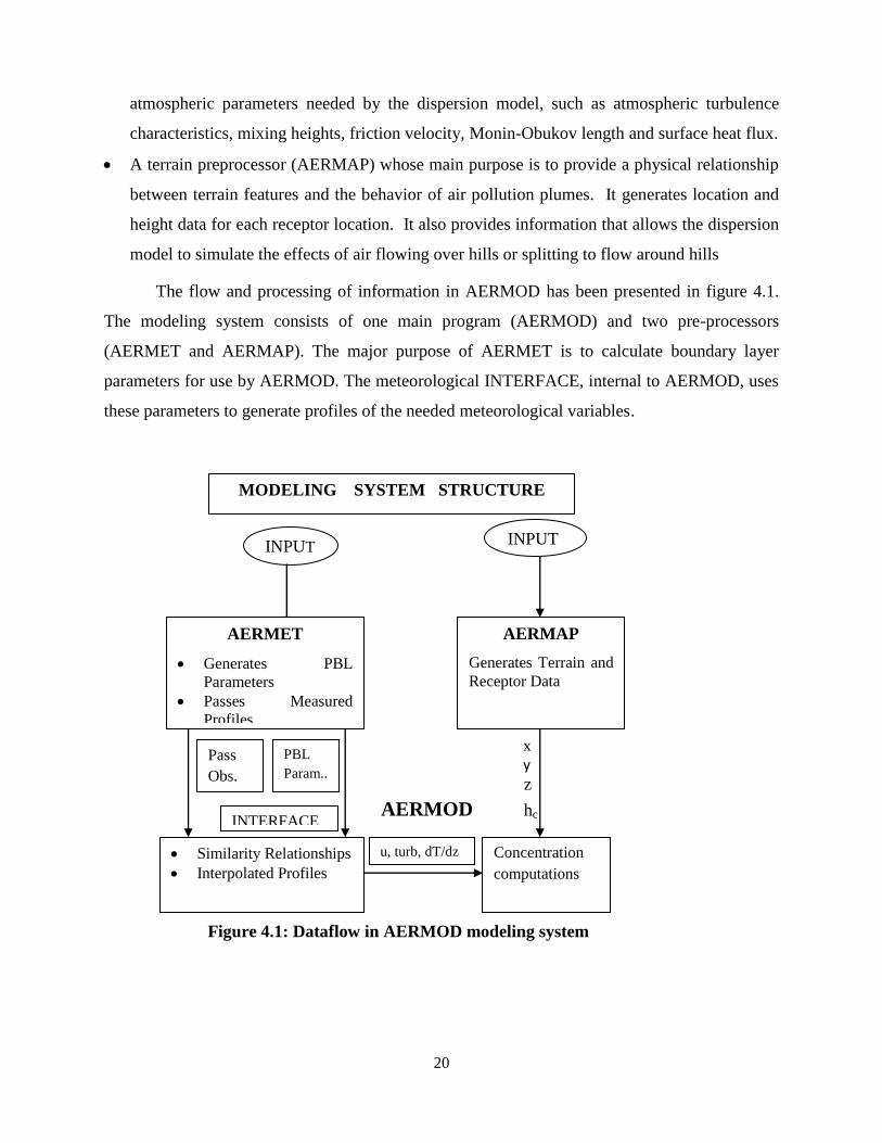
The flow and processing of information in AERMOD has been presented in figure 4.1.

The modeling system consists of one main program (AERMOD) and two pre-processors

(AERMET and AERMAP). The major purpose of AERMET is to calculate boundary layer

parameters for use by AERMOD. The meteorological INTERFACE, internal to AERMOD, uses

these parameters to generate profiles of the needed meteorological variables.

x y

z

AERMOD hc

Figure 4.1: Dataflow in AERMOD modeling system

MODELING SYSTEM STRUCTURE

INPUT

INPUT

AERMET

Generates PBL

Parameters

Passes Measured

Profiles

AERMAP

Generates Terrain and

Receptor Data

Similarity Relationships

Interpolated Profiles

Concentration

computations

INTERFACE

u, turb, dT/dz

PBL

Param..

Pass

Obs.

21

4.2 GENERAL STRUCTURE OF AERMOD

In general, AERMOD models a plume as a combination of two limiting cases: a horizontal

plume (terrain impacting) and a terrain-following plume. Therefore, for all situations, the total

concentration, at a receptor, is bounded by the concentration predictions from these states. The

AERMOD terrain pre-processor (AERMAP) uses gridded terrain data to calculate a

representative terrain-influence height (𝐻𝑐) for each receptor with which AERMOD computes

receptor specific 𝐻𝑐 values. The general concentration equation, which applies in stable or

convective conditions, is given by:

𝐶𝑇 𝑥𝑟 , 𝑦𝑟 , 𝑧𝑟 = f * 𝐶𝑐 ,𝑠 𝑥𝑟 , 𝑦𝑟 , 𝑧𝑟 + 1 − 𝑓 𝑥𝑟 , 𝑦𝑟 , 𝑧𝑝

Where,

𝐶𝑇 𝑥𝑟 , 𝑦𝑟 , 𝑧𝑟 = total concentration

𝐶𝑐 ,𝑠 𝑥𝑟 , 𝑦𝑟 , 𝑧𝑟 = contribution from horizontal plume state

𝐶𝑐 ,𝑠 𝑥𝑟 , 𝑦𝑟 , 𝑧𝑝 = contribution from terrain – following state

𝑓 = plume state weight function

𝑥𝑟 , 𝑦𝑟 , 𝑧𝑟 = co-ordinate representation of a receptor

𝑧𝑝 = height of receptor above local ground = 𝑧𝑟 - 𝑧𝑡

𝑧𝑡 = terrain height at a receptor

4.2.1 Estimation of dispersion coefficients

The overall standard deviations of the lateral and vertical concentration distributions are a

combination of the dispersion resulting from ambient turbulence, and dispersion from turbulence

induced by plume buoyancy. Dispersion induced by ambient turbulence is known to vary

significantly with height, having its strongest variation near the earth’s surface. Unlike present

regulatory models, AERMOD has been designed to account for the effect of variations of

turbulence with height on dispersion through its use of ―effective parameters‖. AERMOD treats

vertical dispersion from ambient turbulence as a combination of a specific treatment for surface

dispersion.

4.2.2 Plume rise calculations in AERMOD

Plume rise in the Convective Boundary Layer (CBL)

The plume rise for the direct source is given by the superposition of source momentum and

buoyancy effects. It is given by:

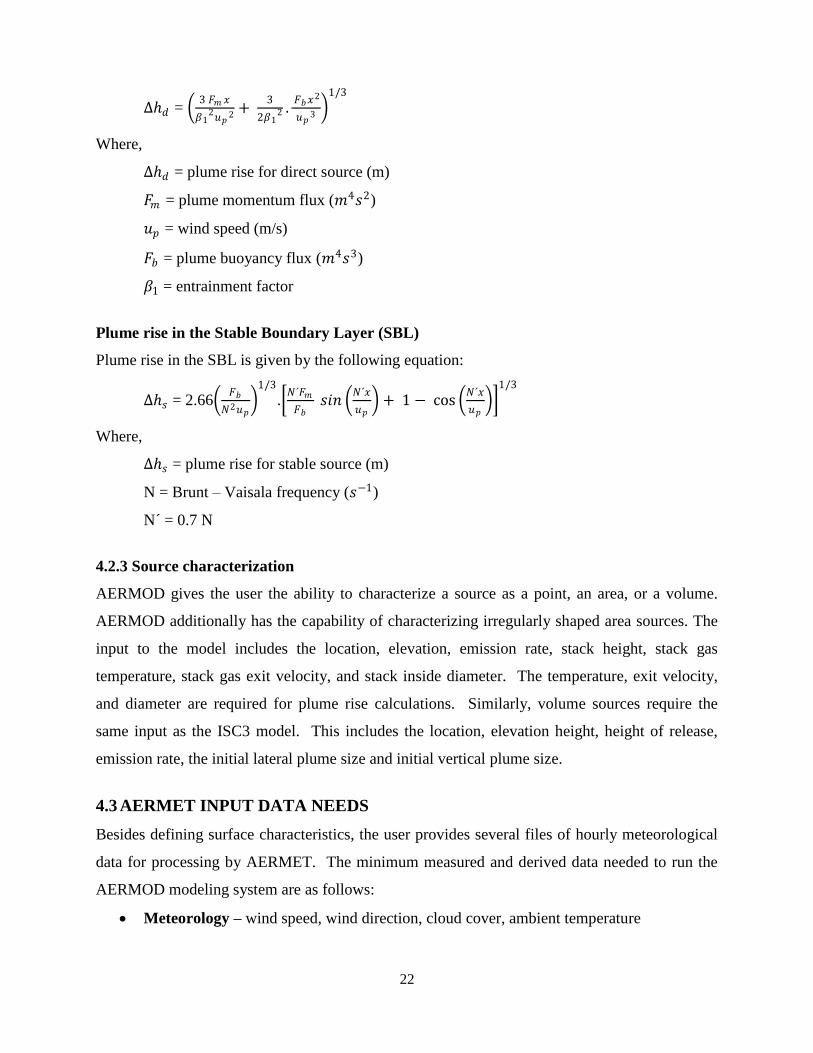
22

∆𝑕𝑑 = 3 𝐹𝑚 𝑥

𝛽12𝑢𝑝

2+

3

2𝛽12 .

𝐹𝑏𝑥2

𝑢𝑝3

1/3

Where,

∆𝑕𝑑 = plume rise for direct source (m)

𝐹𝑚 = plume momentum flux (𝑚4𝑠2)

𝑢𝑝 = wind speed (m/s)

𝐹𝑏 = plume buoyancy flux (𝑚4𝑠3)

𝛽1 = entrainment factor

Plume rise in the Stable Boundary Layer (SBL)

Plume rise in the SBL is given by the following equation:

∆𝑕𝑠 = 2.66 𝐹𝑏

𝑁2𝑢𝑝

1/3

. 𝑁´𝐹𝑚

𝐹𝑏 𝑠𝑖𝑛

𝑁´𝑥

𝑢𝑝 + 1 − cos

𝑁´𝑥

𝑢𝑝

1/3

Where,

∆𝑕𝑠 = plume rise for stable source (m)

N = Brunt – Vaisala frequency (𝑠−1)

N´ = 0.7 N

4.2.3 Source characterization

AERMOD gives the user the ability to characterize a source as a point, an area, or a volume.

AERMOD additionally has the capability of characterizing irregularly shaped area sources. The

input to the model includes the location, elevation, emission rate, stack height, stack gas

temperature, stack gas exit velocity, and stack inside diameter. The temperature, exit velocity,

and diameter are required for plume rise calculations. Similarly, volume sources require the

same input as the ISC3 model. This includes the location, elevation height, height of release,

emission rate, the initial lateral plume size and initial vertical plume size.

4.3 AERMET INPUT DATA NEEDS

Besides defining surface characteristics, the user provides several files of hourly meteorological

data for processing by AERMET. The minimum measured and derived data needed to run the

AERMOD modeling system are as follows:

Meteorology – wind speed, wind direction, cloud cover, ambient temperature

23

Directionally and/or monthly varying surface characteristics – noon time albedo

Bowen’s ratio , roughness length

Other – Latitude, longitude, time zone

Optional – Solar radiation , net radiation , profile of vertical turbulence

4.3.1 Selection and use of measured winds, temperature and turbulence in AERMET

Threshold wind speed

Reference temperature and height

Reference wind speed

Measured turbulence

Data substitution for missing ON-SITE data

4.3.2 Information passed by AERMET to AERMOD: The following information is passed

from AERMET to AERMOD for each hour of the meteorological data recorded:

All observations of wind speed, wind direction, ambient temperature, lateral turbulence &

vertical turbulence with their associated measurement heights.

Sensible heat flux, friction velocity, Monin Obukhov length L, wind direction at the

reference height, ambient temperature at the reference height & the reference height for

temperature.

4.4 AERMAP INPUT DATA NEEDS

The following data is required for AERMAP:

Digital Elevation Model formatted terrain data 𝑥𝑡 , 𝑦𝑡 , 𝑧𝑡

Design of receptor grid; AERMAP accepts polar, Cartesian or discrete receptors.

4.4.1 Information passed by AERMAP to AERMOD

AERMAP passes the following parameters to AERMOD: 𝑥𝑟 , 𝑦𝑟 , 𝑧𝑟 , 𝑧𝑡 and the height scale

(𝑕𝑐 ) for each receptor.

24

4.5 CASE STUDY of AN IRON ORE MINE

It may be observed from the previous sections that the dust dispersion modeling requires the

following data:

Micro – meteorological data

Mining data

Dust concentration data

4.5.1 Meteorological parameters

a. Cloud cover: Cloud cover (also known as cloudiness, cloud amount) refers to the

fraction of the sky obscured by clouds when observed from a particular location. Cloud

cover is expressed either in oktas (or eighths of the sky) or in tenths. They are called

oktas because they are measured with an okta grid. A value of 0 refers to clear sky, while

8 oktas or 10 on the decimal scale indicate overcast. Each okta represents one eighth of

the sky covered by cloud.

b. Global Horizontal radiation: Total solar radiation; the sum of direct, diffuse, and

ground-reflected radiation; however, because ground reflected radiation is usually

insignificant compared to direct and diffuse, for all practical purposes global horizontal

radiation is said to be the sum of direct and diffuse radiation only. Global horizontal

radiation is the sum of both the direct and diffuse components as measured incident on a

flat horizontal plane. It is therefore the sum of the direct horizontal and diffuse

horizontal values.

c. Hourly Precipitation: Precipitation is measured as the depth to which a flat horizontal

surface would have been covered per unit time if no water were lost by runoff,

evaporation, or percolation. Depth is expressed in inches or millimeters. Measuring

precipitation covers rain, hail, snow, rime, hoar frost and fog, and is traditionally

measured using various types of rain gauges such as the non-recording cylindrical

container type or the recording weighing type, float type and tipping-bucket type.

d. Ceiling Height: Ceiling height is defined as the height-above-ground level of the lowest

broken or overcast layer. If the sky is totally obscured, the height of the vertical visibility

(VV) is used as the ceiling height. The height for the lowest broken or overcast layer is

used as the ceiling height.

25

e. Relative humidity: Relative humidity is a term used to describe the amount of water

vapor that exists in a gaseous mixture of air and water vapor.

f. Dry Bulb Temperature: The dry-bulb temperature is the temperature of air measured by

a thermometer freely exposed to the air but shielded from radiation and moisture.

g. Wind Speed: It is the speed of wind, the movement of air or other gases in an

atmosphere.

h. Wind Direction: Wind direction is the direction from which a wind originates. It is

usually reported in cardinal directions or in azimuth degrees.

The ambient air quality was monitored in 12 locations and these have been presented in Figure

4.2. Sample micro-meteorological data for 12 hour period has been presented in Table 4.1.

Figure 4.2: Ambient air quality locations

26

Table 4.1: Micro-meteorological Data

Year Mont

h Day Hr

Cloud

cover

(tenths)

Dry

Bulb

Temp.

(° C)

RH

(%)

Station

Pressure

(mbar)

WD

(deg)

WS

(m/s)

Ceiling

Height

Hourly

ppt

(1/100

of an

inch)

Global

Horizontal

Radiation

(Wh/m2)

2008 10 1 1 4 24.9 70 935 90 3.2 3000 0 0

2008 10 1 2 4 24.9 70 935 225 2.3 3000 0 0

2008 10 1 3 4 24.9 70 935 90 2.9 3000 0 0

2008 10 1 4 4 24.9 70 935 90 2.4 3000 0 0

2008 10 1 5 4 24.9 70 935 135 2.3 3000 0 5000

2008 10 1 6 4 24.9 70 935 135 2.9 3000 0 5000

2008 10 1 7 4 24.9 70 935 315 3.3 3000 0 5000

2008 10 1 8 4 24.9 70 935 0 0 3000 0 5000

2008 10 1 9 4 24.9 70 935 0 0 3000 0 5000

2008 10 1 10 4 24.9 70 935 0 0 3000 0 5000

2008 10 1 11 4 24.9 70 935 0 0 3000 0 5000

2008 10 1 12 4 24.9 70 935 0 0 3000 0 5000

2008 10 1 13 4 24.9 70 935 0 0 3000 0 5000

2008 10 1 14 4 24.9 70 935 315 3.5 3000 0 5000

2008 10 1 15 4 24.9 70 935 90 2.2 3000 0 5000

2008 10 1 16 4 24.9 70 935 90 1.5 3000 0 5000

2008 10 1 17 4 24.9 70 935 135 2.8 3000 0 5000

2008 10 1 18 4 24.9 70 935 225 3.3 3000 0 0

2008 10 1 19 4 24.9 70 935 315 0.8 3000 0 0

2008 10 1 20 4 24.9 70 935 90 3.1 3000 0 0

2008 10 1 21 4 24.9 70 935 90 2.4 3000 0 0

2008 10 1 22 4 24.9 70 935 90 0.8 3000 0 0

2008 10 1 23 4 24.9 70 935 0 0 3000 0 0

2008 10 1 24 4 24.9 70 935 0 0 3000 0 0

27

4.5.2 Mining Data

4.5.2.1 Mining data for Line Source Modeling: The mining data for the line source modeling

for the period is as presented in Table 4.2

Table 4.2: Mining Data for Line Source Modeling

Sl. No. Description Data

1. Production in T /day 6060 T / day

2. Transported material in T / day 6060 T / day

3. Quantity of ore in each trip 35 T

4. No. of trips / day 173 trips

5. No. of trips / hr (8 working hours / day) 22 trips / hr

6. Road width in m 6m

7. Road length in m 6000m

8. Area of pit in 𝑘𝑚2 0.17𝑘𝑚2

9. Moisture Content of Road Dust in % (m) 20

10. Silt Content of road dust in % (s) 10

11. Wind speed in m/sec (u) 2.04

12. Average Vehicle Speed in m/sec (v) 2.7

13. Frequency of vehicle movement in no. per hour (f) 21

14. Capacity of dumpers in ton (c) 35

Haul road emission rate

Haul road emission depends on several factors, which include soil properties, climatic

conditions, vehicular traffic, wind forces and machinery operations. Empirical equation for

calculation of haul road emission rate is given as follows:

E = [{(100 – m) / m} 0.7

{us/ (100 – s)} 0.1

{(41.6 + 0.03 f c + 108v)} 10-5

]

Where

E = Emission rate in g/sec/m

E = 0.008105813 g / sec / m

The haul road emission rate for the mine was found to be 0.0081 g/sec/m.

28

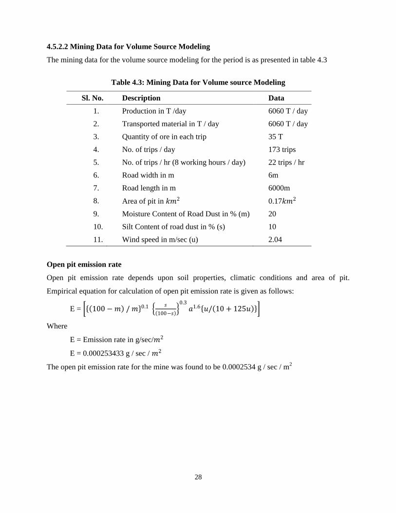
4.5.2.2 Mining Data for Volume Source Modeling

The mining data for the volume source modeling for the period is as presented in table 4.3

Table 4.3: Mining Data for Volume source Modeling

Sl. No. Description Data

1. Production in T /day 6060 T / day

2. Transported material in T / day 6060 T / day

3. Quantity of ore in each trip 35 T

4. No. of trips / day 173 trips

5. No. of trips / hr (8 working hours / day) 22 trips / hr

6. Road width in m 6m

7. Road length in m 6000m

8. Area of pit in 𝑘𝑚2 0.17𝑘𝑚2

9. Moisture Content of Road Dust in % (m) 20

10. Silt Content of road dust in % (s) 10

11. Wind speed in m/sec (u) 2.04

Open pit emission rate

Open pit emission rate depends upon soil properties, climatic conditions and area of pit.

Empirical equation for calculation of open pit emission rate is given as follows:

E = 100 − 𝑚 / 𝑚 0.1 𝑠

100−𝑠

0.3

𝑎1.6 𝑢/ 10 + 125𝑢

Where

E = Emission rate in g/sec/𝑚2

E = 0.000253433 g / sec / 𝑚2

The open pit emission rate for the mine was found to be 0.0002534 g / sec / m2

29

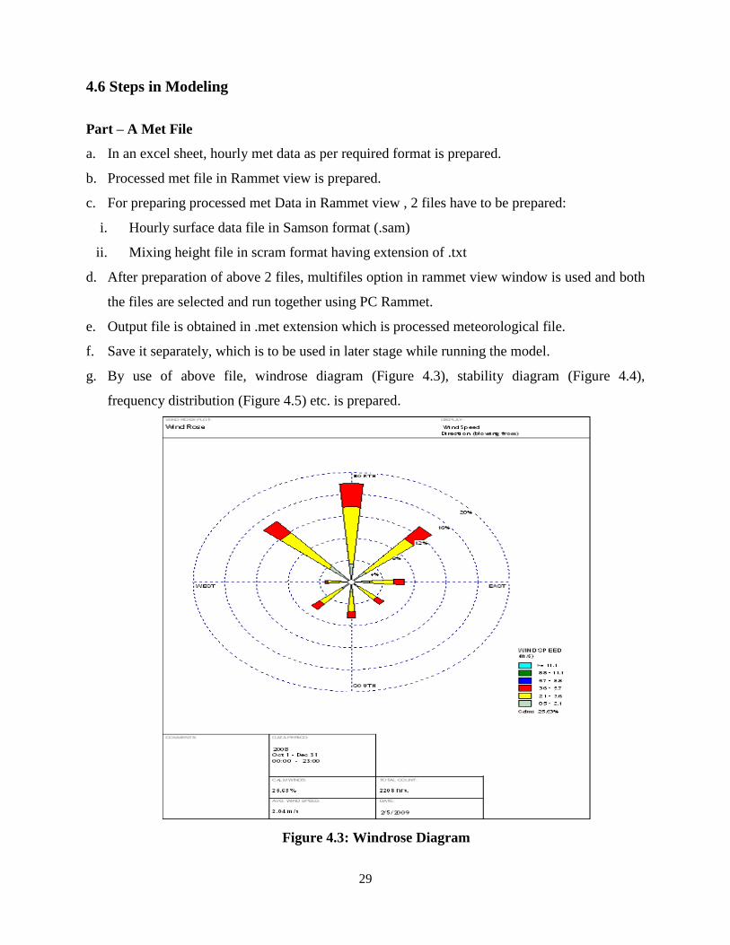
4.6 Steps in Modeling

Part – A Met File

a. In an excel sheet, hourly met data as per required format is prepared.

b. Processed met file in Rammet view is prepared.

c. For preparing processed met Data in Rammet view , 2 files have to be prepared:

i. Hourly surface data file in Samson format (.sam)

ii. Mixing height file in scram format having extension of .txt

d. After preparation of above 2 files, multifiles option in rammet view window is used and both

the files are selected and run together using PC Rammet.

e. Output file is obtained in .met extension which is processed meteorological file.

f. Save it separately, which is to be used in later stage while running the model.

g. By use of above file, windrose diagram (Figure 4.3), stability diagram (Figure 4.4),

frequency distribution (Figure 4.5) etc. is prepared.

Figure 4.3: Windrose Diagram

30

Figure 4.4: Stability Class Diagram

Figure 4.5: Wind Class Frequency Distribution

31

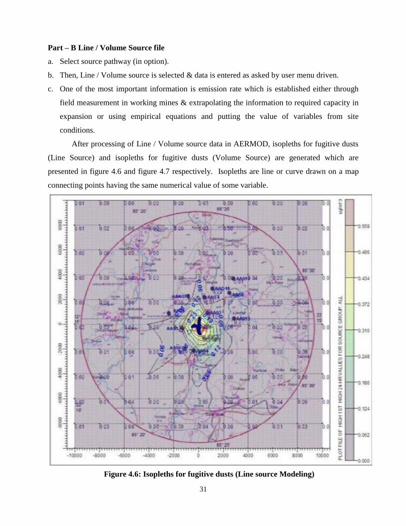
Part – B Line / Volume Source file

a. Select source pathway (in option).

b. Then, Line / Volume source is selected & data is entered as asked by user menu driven.

c. One of the most important information is emission rate which is established either through

field measurement in working mines & extrapolating the information to required capacity in

expansion or using empirical equations and putting the value of variables from site

conditions.

After processing of Line / Volume source data in AERMOD, isopleths for fugitive dusts

(Line Source) and isopleths for fugitive dusts (Volume Source) are generated which are

presented in figure 4.6 and figure 4.7 respectively. Isopleths are line or curve drawn on a map

connecting points having the same numerical value of some variable.

Figure 4.6: Isopleths for fugitive dusts (Line source Modeling)

32

Figure 4.7: Isopleths for fugitive dusts (Line source Modeling)

33

CHAPTER 5

DISCUSSION AND CONCLUSION

34

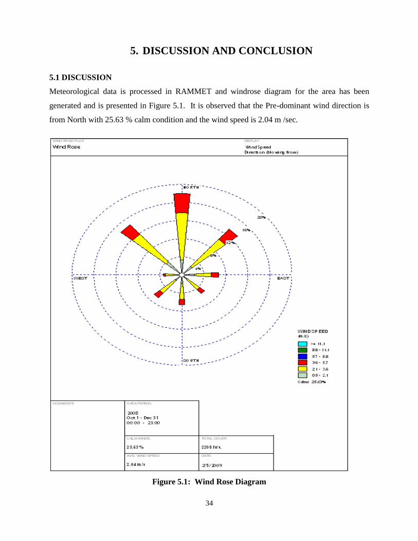
5. DISCUSSION AND CONCLUSION

5.1 DISCUSSION

Meteorological data is processed in RAMMET and windrose diagram for the area has been

generated and is presented in Figure 5.1. It is observed that the Pre-dominant wind direction is

from North with 25.63 % calm condition and the wind speed is 2.04 m /sec.

Figure 5.1: Wind Rose Diagram

35

Windrose showing Stability class is also generated and is presented in figure 5.2.

Stability Class was found to be F.

Figure 5.2: Stability Class

36

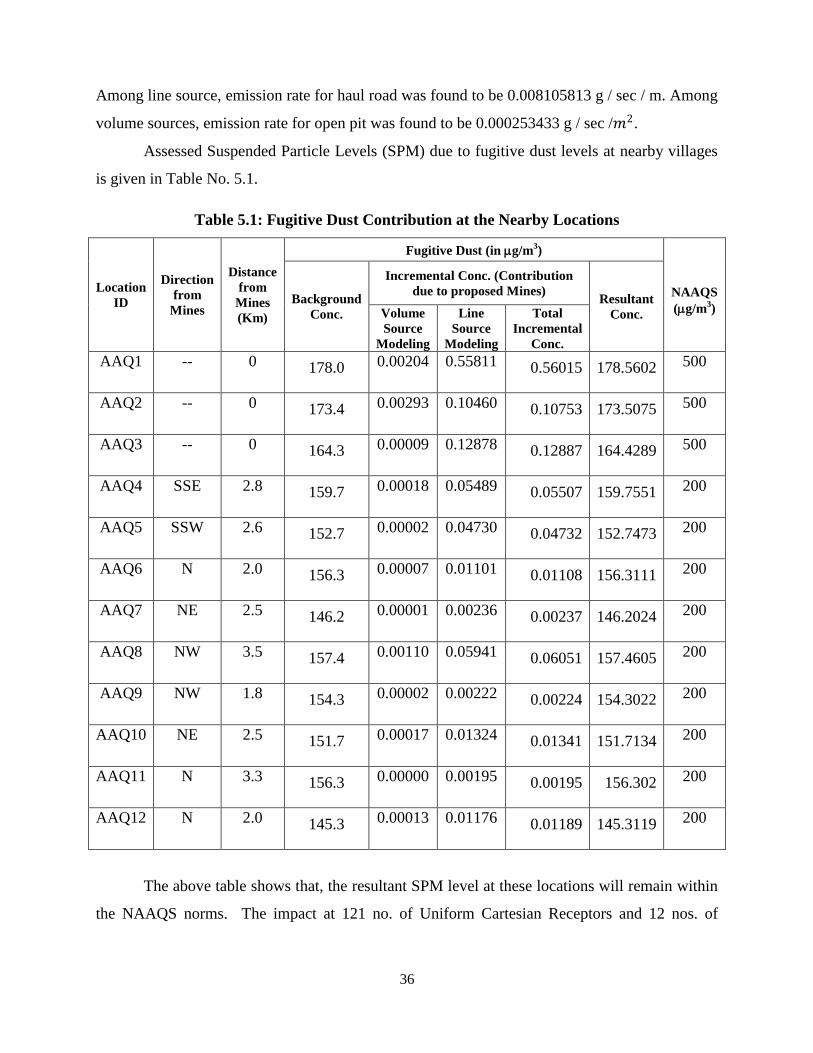
Among line source, emission rate for haul road was found to be 0.008105813 g / sec / m. Among

volume sources, emission rate for open pit was found to be 0.000253433 g / sec /𝑚2.

Assessed Suspended Particle Levels (SPM) due to fugitive dust levels at nearby villages

is given in Table No. 5.1.

Table 5.1: Fugitive Dust Contribution at the Nearby Locations

Location

ID

Direction

from

Mines

Distance

from

Mines

(Km)

Fugitive Dust (in g/m3)

NAAQS

(g/m3)

Background

Conc.

Incremental Conc. (Contribution

due to proposed Mines) Resultant

Conc. Volume

Source

Modeling

Line

Source

Modeling

Total

Incremental

Conc.

AAQ1 -- 0 178.0 0.00204 0.55811 0.56015 178.5602 500

AAQ2 -- 0 173.4 0.00293 0.10460 0.10753 173.5075 500

AAQ3 -- 0 164.3 0.00009 0.12878 0.12887 164.4289 500

AAQ4 SSE 2.8 159.7 0.00018 0.05489 0.05507 159.7551 200

AAQ5 SSW 2.6 152.7 0.00002 0.04730 0.04732 152.7473 200

AAQ6 N 2.0 156.3 0.00007 0.01101 0.01108 156.3111 200

AAQ7 NE 2.5 146.2 0.00001 0.00236 0.00237 146.2024 200

AAQ8 NW 3.5 157.4 0.00110 0.05941 0.06051 157.4605 200

AAQ9 NW 1.8 154.3 0.00002 0.00222 0.00224 154.3022 200

AAQ10 NE 2.5 151.7 0.00017 0.01324 0.01341 151.7134 200

AAQ11 N 3.3 156.3 0.00000 0.00195 0.00195 156.302 200

AAQ12 N 2.0 145.3 0.00013 0.01176 0.01189 145.3119 200

The above table shows that, the resultant SPM level at these locations will remain within

the NAAQS norms. The impact at 121 no. of Uniform Cartesian Receptors and 12 nos. of

37

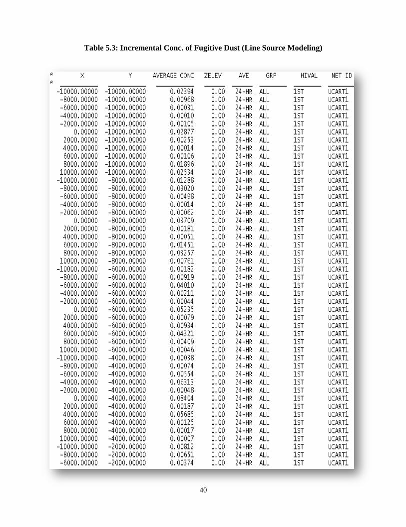
Discrete Cartesian Receptors in the study area due to mining activity (Volume Source Modeling)

and Transportation (Line Source Modeling) are presented in the Table 5.2 & Table 5.3.

TABLE 5.2: Incremental Conc. of Fugitive Dust (Volume Source Modeling)

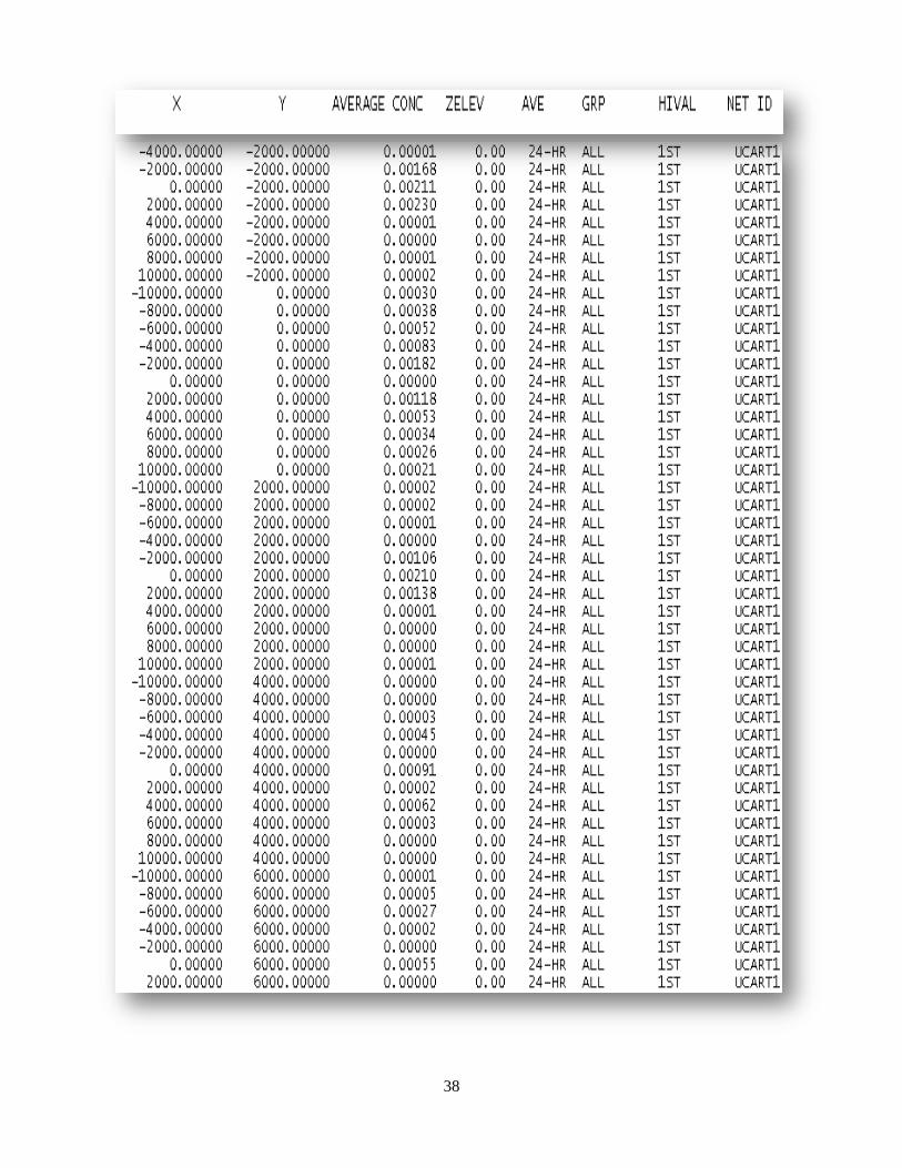
38

39

40

Table 5.3: Incremental Conc. of Fugitive Dust (Line Source Modeling)

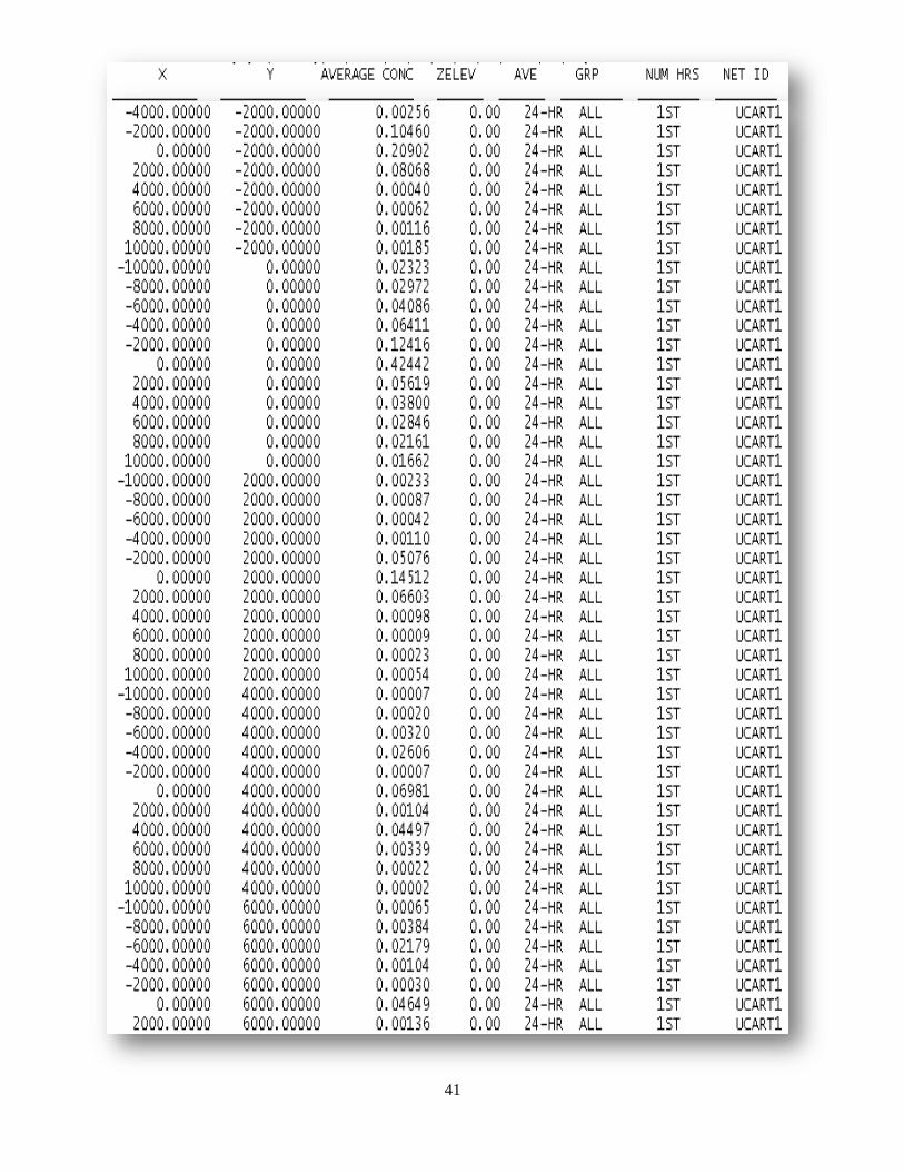
41

42

43

SPM and RPM are the major sources of emission from various open pit mining activities. The

annual and 24-Hr average concentrations of SPM and RPM are lower than the NAAQS at

mining and residential places. In order to reduce the effect of SPM and RPM a few additional

measures may be implemented.

Restriction of trucks/dumpers speed and overhauling, and regular road cleaning are

essential in order to control dust pollution from transportation, together with water spraying on

roads. Washing of dumpers / trucks’ wheels/body at an appropriate distance from site entrance,

loading and unloading in area protected from wind, minimization of drop heights, use of sheet or

cover on loaded vehicles and application of water sprays to moisten transported material is also

essential.

Installation of sprinkling system along with application of binding agents, chemicals on

unpaved roads are required. In addition, unpaved roads should be converted to black topped

roads, with regular maintenance/ repair of roads to maintain compactness, gradient and drainage,

sweeping of unpaved roads and the imposition of speed limits on trucks and other vehicles.

A Green belt should be developed having plants with thick foliage, which will effectively

attenuate the dust concentration.

5.2 CONCLUSION

Air quality modeling has been attempted using AERMOD. Line source & Volume source

modeling has been carried out for haul road and open pit respectively. Wind rose and stability

class diagram for the area for the monitoring period has been generated. From the modeling

exercise, dust concentrations at certain receptor locations have been predicted and it was found

that the resultant SPM level at these locations will remain within the NAAQS norms. With use

of meteorological data, dust concentration data and emission data, isopleths for mining area

could be generated using AERMOD. AERMOD could be used not only for existing mines but

for also proposed mines. It can predict dust concentrations and accordingly measures for dust

control could be adopted.

44

CHAPTER 6

REFERENCES

45

6. REFERENCES

Chaulya, S.K., Ahmad M, Singh RS, Bandopadhyay LK, Bondyopadhay C, Mondal GC., 2003,

―Validation of two air quality models for Indian mining conditions‖, Environmental

Monitoring and Assessment, February, Volume 82(1); pp. 23 – 43

Chaulya, S.K., 2005, ―Air Quality status of an Open Pit Mining Area in India‖, Environment

Monitoring and Assessment, Vol. 105, pp. 369 – 389

Cole, C.F. and Fabrick, A.J., 1984, ―Surface mine pit retention‖, Journal of Air Pollution Control

Assoc 34(6):674–675.

EPA, 1995a, User's guide for the industrial source complex (ISC3) dispersion models. Vol. I.

User instructions. Research Triangle Park, NC: U.S. Environmental Protection Agency,

Office of Air Quality Planning and Standards, Emissions, Monitoring, and Analysis

Division, EPA publication No. EPA–454/B–95–003a.

EPA,1995b, User's guide for the industrial source complex (ISC3) dispersion models. Vol. II.

Description of model algorithms. Research Triangle Park, NC: U.S. Environmental

Protection Agency, Office of Air Quality Planning and Standards, Emissions, Monitoring,

and Analysis Division, EPA publication No. EPA–454/B–95–003b.

Ghose, M. K, Majee, S.R., 2000, " Assessment of dust generation due to opencast coal mining –

An Indian Case Study‖, Environmental Monitoring and Assessment, Volume 61; pp. 255–

263

Pereira, M.J, Soares A, Branquinho, C, 1997, Stochastic simulation of fugitive dust emissions.

In: Baafi EY, Schofield NA, eds. Wollongong '96, Fifth International Geostatistics

Congress. Vol. 2. Dordrecht, Netherlands: Kluwer Academic Publishers, pp. 1055–1065.

Reed, W.R., 2005, ―Significant Dust Dispersion Models for Mining Operations‖, Information

Circular 9478, DHHS (NIOSH) Publication No. 2005 –138

Reed, W.R., 2004, ―Performance Evaluation of a Dust-Dispersion Model for Haul Trucks ", The

National Institute for Occupational Safety and Health (NIOSH), Transactions of Society for

Mining, Metallurgy, and Exploration

Reed, W.R., 2003, An improved model for prediction of PM10 from surface mining operations

[Dissertation]. Blacksburg, VA: Virginia Polytechnic Institute and State University,

Department of Mining and Minerals Engineering.

Singh, G., Prabha, J., Giri, S., 2006, ―Comparison and performance evaluation of dispersion

models FDM and ISCST3 for a gold mine at Goa, Journal of Industrial pollution control ;

Volume 22(2) ; pp. 297 – 303

Singh, G., Prabha, J., Sinha, I.N, 2006, ―Emission factor equations for haul roads: The Indian

Perspective‖, Indian Journal of Air Pollution Control; Volume 6, No. 1; pp .37 – 43

Trivedi, R. , Chakraborty , M.K. , 2008, ―Dust generation and its dispersion due to mining

activities in Durgapur open cast coal project of W.C.L. – A Case Study‖, The Indian

Mining & Engineering Journal, February, pp. 24 – 31

46

Trivedi , R. , Chakraborty, M.K., Tewary ,B.K., 2009, ―Dust Dispersion Modeling using fugitive

dust model at an opencast coal project of Western Coalfields Limited, India‖, Journal of

Scientific & Industrial Research, Volume 68, January pp. 71 – 78

Trivedi , R. , Chakraborty, M.K., Tewary ,B.K.,2008, ― A Study Dust Dispersion of Air borne

Dust Generated due to Mining Activities in Gughus Opencast coal project , W.C.L‖,

Conference on Emerging Trends in Mining and Allied Industries , February, pp. 227 – 236

www.epa.gov/scram001/7thconf/aermod/aermod_mfd.pdf

www.lete.poli.usp.br/Guenther/aula_4/Plumes.pdf

www.yosemite.epa.gov/oaqps/EOGtrain.nsf/fabbfcfe2fc93dac85256afe00483cc4/c9862a32b0eb

4f9885256b6d0064ce2b/$FILE/Lesson%206.pdf

http://atmospheric-pollution.blogspot.com/2007/04/briggs-plume-rise-equations-i.html