beam forming and adaptive beam forming techniques and its...

IOSR Journal of VLSI and Signal Processing (IOSR-JVSP)

Volume 3, Issue 5 (Nov. – Dec. 2013), PP 07-17 e-ISSN: 2319 – 4200, p-ISSN No. : 2319 – 4197

www.iosrjournals.org

www.iosrjournals.org 7 | Page

Beam forming and Adaptive beam forming Techniques and its

implementation on ADSP TS 201 Processor

Prasanth .CR1, Sreeja K.S

2,Nidheesh.H

3, Prince Joseph

4

1Pursing Mtech at college of Engineering cherthala 2Pursing Mtech at college of Engineering cherthala 3Pursing Btech at college of Engineering cherthala 4Pursing Btech at college of Engineering cherthala

Abstract: Digital signal processing (DSP) is concerned with the representation of discrete time signals by a

sequence of numbers or symbols and the processing of these signals. Digital signal processing and analog

signal processing are subfields of signal processing. DSP includes subfields like: audio and speech signal

processing, sonar and radar signal processing, sensor array processing, spectral estimation, statistical signal

processing, digital image processing, signal processing for communications, control of systems, biomedical

signal processing, seismic data processing, etc. in this paper mainly concentrate on array signal processing. Array processing involves combining all sensor outputs in some optimal manner so that the coherent signals

emitted by the source are received and all other inputs are maximally discarded. Beam forming algorithms are

the foundation for all array processing techniques since this is an effective technique to estimate direction of

arrival (DOA). The areas in which beam formers play an important role include radar, sonar, seismology etc. in

this paper presents comparative study of beam forming techniques and its implementation on ADSP TS 201

processor

Keywords: signal-to-interference-plus-noise ratio (SINR), direction of arrival (DOA), Minimum

Variance Distortion less Response (MVDR),

I. Introduction The goal of DSP is usually to measure, filter and/or compress continuous real-world analog

signals. The first step is usually to convert the signal from an analog to a digital form, by sampling and then

digitizing it using an analog-to-digital converter (ADC), which turns the analog signal into a stream of numbers.

However, often, the required output signal is another analog output signal, which requires a digital-to-analog

converter (DAC). Even if this process is more complex than analog processing and has a discrete value range,

the application of computational power to digital signal processing allows for many advantages over analog processing in many applications, such as error detection and correction in transmission as well as data

compression DSP algorithms have long been run on standard computers, on specialized processors called digital

signal processor on purpose-built hardware such as application-specific integrated circuit (ASICs). Today

there are additional technologies used for digital signal processing including more powerful general purpose

microprocessors, field-programmable gate arrays (FPGAs), digital signal controllers (mostly for industrial apps

such as motor control), and stream processors, among others.

In DSP, processing is done in one of the following domains: time domain (one-dimensional signals),

spatial domain (multidimensional signals), frequency domain, and wavelet domains. We choose the domain to

process a signal in by making an informed guess as to which domain best represents the essential characteristics

of the signal. A sequence of samples from a measuring device produces a time or spatial domain representation,

whereas a discrete Fourier transform produces the frequency domain information that is the frequency spectrum.

Array processing is signal processing of the outputs of an array of sensors to:

Enhance the signal-to-interference-plus-noise ratio (SINR) compared to that of a single sensor using

conventional or adaptive beam forming.

Determine the number of emitting sources, the locations of these sources, their waveforms, and other

signal parameters.

Track multiple moving sources.

Array processing is used in radar, sonar, seismic exploration, anti-jamming and wireless communications. One

of the main advantages of using array processing along with an array of sensors is a smaller foot-print. The

problems associated with array processing include the number of sources used, their direction of arrivals, and

their signal waveforms.

http://en.wikipedia.org/wiki/Signal_processing

http://en.wikipedia.org/wiki/SINR

http://en.wikipedia.org/wiki/Sensor

http://en.wikipedia.org/wiki/Beamforming

http://en.wikipedia.org/wiki/Waveforms

http://en.wikipedia.org/wiki/Radar

http://en.wikipedia.org/wiki/Sonar

http://en.wikipedia.org/wiki/Wireless

http://en.wikipedia.org/wiki/Direction_of_arrival

http://en.wikipedia.org/wiki/Waveforms

Beam forming and Adaptive beam forming Techniques and its implementation on ADSP TS 201


An array is used to filter signals in a space-time field by exploiting their spatial characteristics. In this

paper we have limited the application of beam formers in passive acoustic systems. Passive array elements listen

to the incoming acoustic energy and use it to estimate the temporal and spatial characteristics of the observed signal field. The most important application is the detection and tracking of the underwater systems. The

spatially sampled time series from each sensor is linearly combined in beam former to obtain a scalar output

time in the same manner that an FIR filter linearly combines temporally sampled data. The design of the arrays

to achieve certain performance criteria involves tradeoffs among array geometry, the number of sensors, signal

to noise ratios, signal to interference ratios, as well as a number of other factors.

The most commonly used array geometries are:

Linear Arrays (LA): In linear arrays, sensors are located at arbitrary points on a line. Linear arrays may be

classified into uniform and non-uniform linear arrays. In uniform linear arrays (ULA), the distance between the

sensors will be uniform. Non-uniform linear arrays have unequal spacing between elements.

Planar Array: A planar array is an array whose elements all lie in the xy-plane. Some of the possible array

geometries are rectangular arrays, circular arrays and hexagonal arrays. Volumetric Array: In volumetric arrays the physical location of the sensors must conform to the shape of the

curved surface they are mounted on. The commonly used geometries are spherical and cylindrical.

1.1 Uniform Linear Array (ULA) Here we focus on Uniform Linear Array (ULA), which is an array that has all its elements on a line with

equal spacing between the elements. For the ULA, the inter element spacing is denoted by d. The inter element

spacing d is simply the spatial sampling interval, which is the inverse of the sampling frequency. Therefore, similar to Shannon‟s theorem for discrete-time-sampling, there are certain requirements on the spatial sampling

frequency to avoid aliasing. Since normalized frequencies are unambiguous is -90˚≤ Φ ≤ 90˚, the sensor

spacing must be

d ≤ λ/2

to prevent spatial ambiguities. Here λ is the wavelength of the propagating wave. Since lowering the array

spacing below this upper limit only provides redundant information and directly conflicts with the desire to have

as much aperture as possible for a fixed number of sensors.

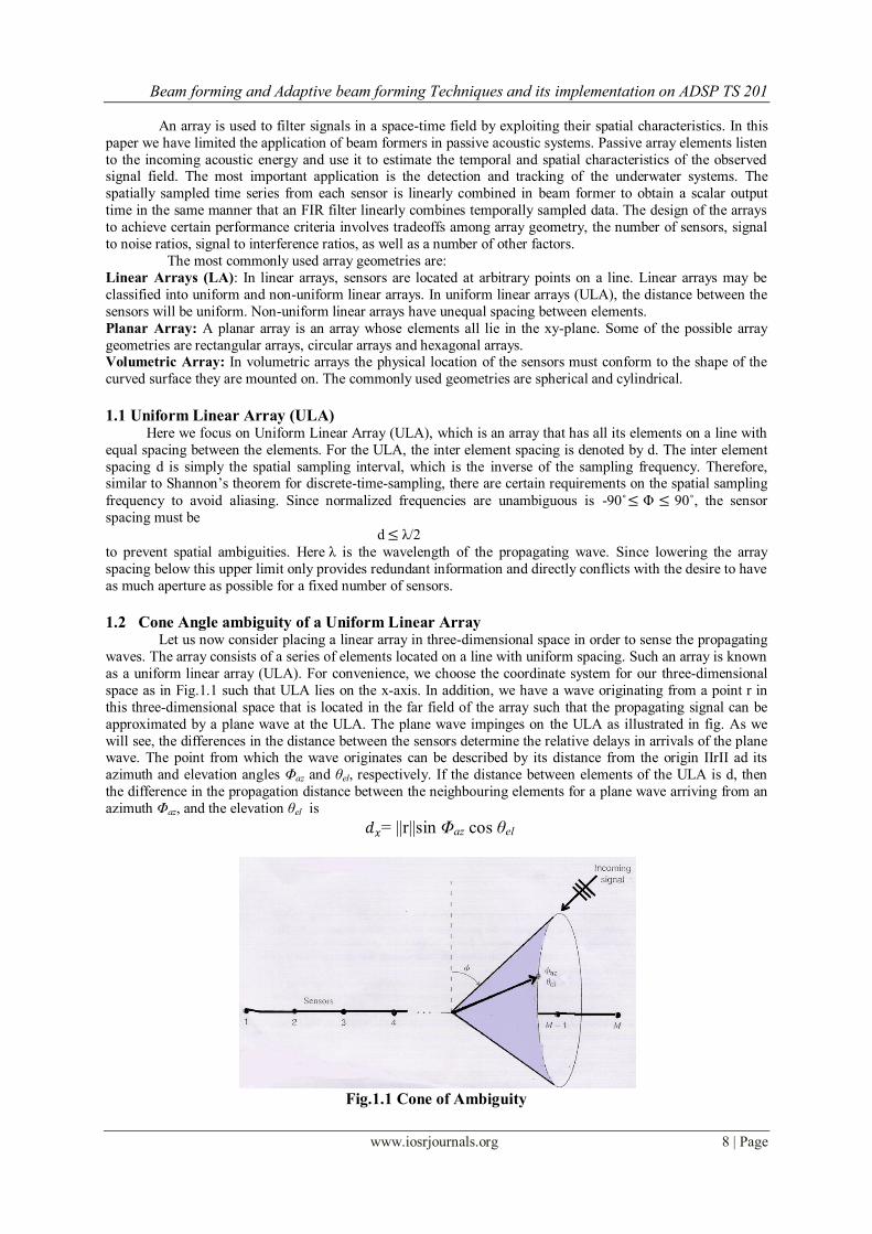
1.2 Cone Angle ambiguity of a Uniform Linear Array Let us now consider placing a linear array in three-dimensional space in order to sense the propagating

waves. The array consists of a series of elements located on a line with uniform spacing. Such an array is known

as a uniform linear array (ULA). For convenience, we choose the coordinate system for our three-dimensional

space as in Fig.1.1 such that ULA lies on the x-axis. In addition, we have a wave originating from a point r in

this three-dimensional space that is located in the far field of the array such that the propagating signal can be

approximated by a plane wave at the ULA. The plane wave impinges on the ULA as illustrated in fig. As we

will see, the differences in the distance between the sensors determine the relative delays in arrivals of the plane wave. The point from which the wave originates can be described by its distance from the origin IIrII ad its

azimuth and elevation angles Φaz and θel, respectively. If the distance between elements of the ULA is d, then

the difference in the propagation distance between the neighbouring elements for a plane wave arriving from an

azimuth Φaz, and the elevation θel is

𝑑𝑥= ||r||sin Φaz cos θel

Fig.1.1 Cone of Ambiguity



These differences in the propagation distance that the plane wave must travel to each of the sensors are

a function of a general angle of arrival with respect to the ULA. If we consider the entire three-dimensional

space, we note that equivalent delays are produced by any signal arriving from a cone about the ULA. Therefore, any signal arriving at the ULA on this surface has the same set of relative delays between the

elements. This conical ambiguity surface is illustrated in the figure. For this reason, the angle of incidence to a

linear array is commonly referred to as the cone angle, Φcone. We see that the cone angle is related to the

physical angles, azimuth and elevation defined in the figure by

sinΦ= sinΦaz Cosθel

where Φ=90- Φcone.

1.3 Beamforming: Conventional and Adaptive Passive arrays use beamforming techniques to detect presence and direction of arrival of underwater

sound sources. One of the simplest non-parametric DOA estimation methods is commonly referred to as the

conventional beamformer. It is based on scanning the array beam and computing the output power for each

beam scan angle. Although the conventional beamformer is rather limited in its angular resolution, its significant

advantages are implementation simplicity and robustness.

To overcome the low resolution property of the conventional beamformer, we estimate the spatial

spectrum of multiple sources by means of a spatial filter that maintains a distortionless response towards the

signal coming from the direction „Ɵ‟ while minimizing the total array output power. Minimum variance

distortion less response is an adaptive algorithm which will minimise the output in all directions subject to the

condition that gain in the steering direction is unity. The steering direction is the bearing that the array is steered towards to look for a particular incoming signal. This algorithm gives optimum performance by steering nulls in

the direction of interference and also offers better performance in the case of correlated noise sources. The

traditional design approaches to adaptive beamforming do not provide sufficient robustness and are not

applicable in situations like small sample size, imprecise knowledge of the desired steering vector etc. Thus

various robust adaptive beamforming techniques gained a significant popularity due to their practical

importance. The most popular conventional robust adaptive technique is the diagonal loading technique.

II. Beamforming

A beamformer is a spatial filter that processes the data obtained from an array of sensors in a manner that serves to enhance the amplitude of the desired signal wave front relative to background noise and

interference. Signals from a particular angle or a set of angles are enhanced by constructive combination and

noise from other angles is rejected by destructive interference. Spatial discrimination capability depends on the

size of the spatial aperture, as the aperture increases, the discrimination improves.

For computation of the delays the sensors need to be represented in a three dimensional co-ordinate

system, i.e. each sensor position is represented by a 3D vector. Consider a group of M sensors located in the

space, whose position vector is given by {𝑟𝑖 ,i= 1, 2…M} Each 𝑟𝑖 is a 3D vector representing the x, y, z co-

ordinates of the sensor, with reference to the origin. Let s(n)=𝑒𝑗2𝜋

𝑓𝑛𝑓𝑠 be the complex sinusoid prpagating through

the medium with a unit direction vector u . The time delayed signal received at the ith sensor is

xi (n)=exp[j(2Л𝑓𝑛

𝑓𝑠+ kri.u)], i=1,2…..M Eq(2.1)

Where k =2𝜋𝑓

𝑐 is the wave number, fs is the sampling frequency and c is the speed of sound in water (1500m/s).

Summing these signals yields

y(n) = 𝑥𝑖𝑀𝑖=1 𝑛 = 𝑒

𝑗2𝜋𝑓𝑛𝑓𝑠 𝑒𝑗𝑘𝑟 𝑖 .𝑢 𝑀

𝑖=1 where 𝑒𝑗 𝑘𝑟 𝑖 .𝑢𝑀𝑖=1 Eq(2.2)

is termed as the complex Beam Pattern, b(f,u) and

ri.u = rxi cosΦcosθ + ryi sinΦcosθ+rzi sinθ Eq(2.3)

where θ is the elevation angle and Φ is the azimuth angle.

For one dimensional array, ri = {(i-1) d, 0, 0},i=1,2…..M Fig 2.1 shows a one dimensional linear array of sensors.



Fig.2.1 Plane wave impinging on a uniform linear array

Plane wave impinging on a uniform linear array

y(n) = 𝑒𝑗2𝜋

𝑓𝑛𝑓𝑠 exp[𝑗𝑘 𝑖 − 1 𝑑 cos 𝜃 𝑐𝑜𝑠ɸ]𝑀

𝑖=1 Eq(2.4)

The projection of the signal directional u on the x-axis can be represented by a conic angle Ψ, where sin Ψ =

cosɸ cosθ. The magnitude of the summation in Eq()

i.e. exp[𝑗𝑘 𝑖 − 1 𝑑 cos 𝜃 𝑐𝑜𝑠ɸ]𝑀𝑖=1 can be written as

𝑏(𝑓, 𝑢) = sin 𝜋𝑓𝑀𝑑 𝑠𝑖𝑛𝛹 /𝑐]

sin 𝜋𝑓𝑑 𝑠𝑖𝑛𝛹 /𝑐] =M, when Ψ= 00. Eq(2.5)

For a given frequency, a plane wave with a conic angle Ψ not equal to zero is attenuated. A plane wave with

a conic angle of zero degree arrives at all M sensors simultaneously, so the outputs of these sensors are added

coherently or in phase. For simulation purpose a linear array of 32 sensors with 0.45λ spacing is considered.

From the above results it is clear that the beam forming operation is maximum at “broadside”(plane wave

parallel to the array). To add the sensor signals coherently (i.e., in phase) for an arbitrary direction vector, uo , projection of the vector,(u-u0) on the sensor position vectors, ri , i=1,2……….M is calculated .

Therefore y(n)= 𝑒𝑗2𝜋

𝑓𝑛𝑓𝑠 𝑒𝑗𝑘 𝑟𝑖 .(𝑢−𝑢0)𝑀

𝑖=1 Eq(2.6)

Hence 𝑏(𝑓, 𝑢) = sin 𝜋𝑓𝑀𝑑 (𝑠𝑖𝑛𝛹 − 𝑠𝑖𝑛𝛹0 /𝑐]

sin 𝜋𝑓𝑑 (𝑠𝑖𝑛𝛹 − 𝑠𝑖𝑛𝛹0 /𝑐] Eq(2.7)

Fig 2.2 shows the beampattern steered to 500.

Fig.2.2 Beampattern for source at 50

0

III. Conventional Beamforming

3.1 Time domain beamforming Beamforming operation can be performed in time domain as well as in frequency domain. The

simplest approach to beamforming is conventional delay and sum beamforming. The under lying idea is very

simple: if a propagating signal is present in an array‟s apperture, sensor outputs ,delayed by appropriate amounts

add together ,reinforce the signal with respect to noise or waves propagating in different directions. The delays

that reinforce the signals are directly related to the length of time it takes for the signal to propagate between

sensors.



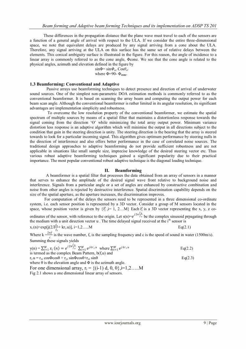
Fig 3.1 shows the block diagram of the conventional delay and sum beamformer in time domain. Here, inputs

from each sensor are shifted so that the signals are aligned in time and are then added.

Fig.3.1 Conventional delay and sum beamformer

However the delays are generally not integer multiples of the sampling period T sec,we cannot form sums that

involve sensor signals delayed by non integer multiple of T .To reduce the aberrations introduced by delay

quantization, we can interpolate between the samples of the sensor signals. Two such approaches can be

followed.

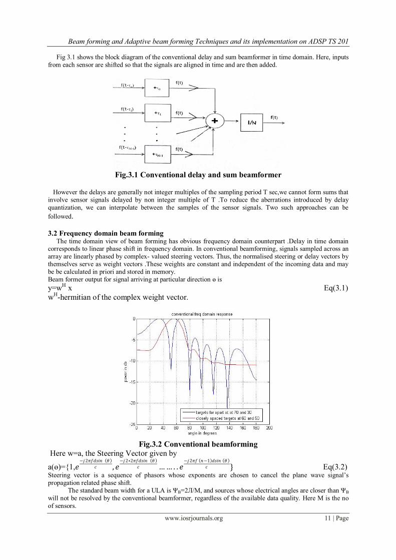
3.2 Frequency domain beam forming The time domain view of beam forming has obvious frequency domain counterpart .Delay in time domain corresponds to linear phase shift in frequency domain. In conventional beamforming, signals sampled across an

array are linearly phased by complex- valued steering vectors. Thus, the normalised steering or delay vectors by

themselves serve as weight vectors .These weights are constant and independent of the incoming data and may

be be calculated in priori and stored in memory.

Beam former output for signal arriving at particular direction ɵ is

y=wH x Eq(3.1)

wH-hermitian of the complex weight vector.

Fig.3.2 Conventional beamforming

Here w=a, the Steering Vector given by

a(ɵ)={1,𝑒−𝑗2𝜋𝑓𝑑𝑠𝑖𝑛 𝜃

𝑐 , 𝑒−𝑗2∗2𝜋𝑓𝑑𝑠𝑖𝑛 𝜃

𝑐 … … . . 𝑒−𝑗2𝜋𝑓 𝑛−1 𝑑𝑠𝑖𝑛 𝜃

𝑐 } Eq(3.2) Steering vector is a sequence of phasors whose exponents are chosen to cancel the plane wave signal‟s

propagation related phase shift.

The standard beam width for a ULA is ΨB=2Л/M, and sources whose electrical angles are closer than ΨB

will not be resolved by the conventional beamformer, regardless of the available data quality. Here M is the no

of sensors.



IV. Adaptive Beamforming

Adaptive beamforming optimizes a collection of weight vectors to localize targets via correlation with the

data in a noisy environment. These weight vectors generate a beampattern that places nulls in the direction of

unwanted noise (i.e., signals, called interference, from directions other than the direction of interest). In contrast

to conventional beamforming where the weight vector is a constant and independent of incoming data ,Adaptive

Beamforming (ABF) algorithms use information about the cross spectral density matrix (CSM) to compute the

weights in such a way so as to improving the beamforming output.

4.1 Minimum Variance Distortionless Response (MVDR) Minimum variance distortion less response is an adaptive algorithm which will minimise the output

in all directions subject to the condition that gain in the steering direction is unity. The steering direction is the

bearing that the array is steered towards to look for a particular incoming signal. This algorithm gives optimum

performance by steering nulls in the direction of interference and also offers better performance in the case of

correlated noise sources.

Consider a narrow band beamformer with a signal arriving from angle 𝜃. The signals arriving from the

different array elements are transformed into the frequency domain using the discrete Fourier transform (DFT).

Let this input vector be x. The scalar output for a Particular direction ɵ can be expressed as

y(k)=𝑤𝐻 .x(k) Eq(4.1)

where k is the time index , x(k)=[x1(k),….xM( k)]Tϵ 𝐶𝑀×1 is the complex vector of array observations ,w

=[𝑤1,…………….𝑤𝑚]T ϵ 𝐶𝑀×1 is the complex vector of beamformer weights , 𝑤𝐻 denotes its complex-conjugate

transposition and and M is the number of array sensors. The observation vector is given by,

X(k)= s(k) +i(k)+n(k)=s(k)a+i(k)+n(k) Eq( 4.2)

Where s(k) ,i(k) and n(k) are the desired signal , interference and noise components respectively. Here s(k) is the

signal waveform , and a is the signal steering vector.

The weight vector can be found from the maximum of the signal-to-interference plus noise ratio(SINR)

SINR = 𝜎𝑠

2 𝑤 𝐻𝑎

𝑤 𝐻𝑅𝑖+𝑛 𝑤

2

Eq(4.3)

Where Ri+n =E{(i(k)+n(k))(i(k)+n(k))H} Eq(4.4)

is the MxM cross spectral density matrix.

The power at the beamformer output is given by and 𝜎𝑠2 is the signal power. It is easy to find the solution

for the weight vector by maintaining a distortion less response toward the desired signal and minimising the

output interference plus noise power. Hence the maximisation of Eq(4.3) is equivalent to Min wH Ri+nw subject to wHa=1 Eq(4.5)

The MVDR weight vector are obtained by the Lagrange multiplier method as

W(𝜃)=𝑅𝑖+𝑛

−1 𝑎(𝜃)

𝑎𝐻 𝜃 𝑅𝑖+𝑛−1 𝑎(𝜃 )

Eq(4.6)

P= E{ 𝑦2 } = 𝑤𝐻𝐸 𝑥. 𝑥𝐻 𝑤 = 𝑤𝐻𝑅𝑤 Eq(4.7)



The optimum MVDR weights calculated above is for narrow band sources. Broadband processing involves

calculation of the beamformer output for multiple frequency bins, as opposed to narrowband MVDR where only

one frequency bin is processed. After the power output has been obtained for each frequency bin ,these individual outputs are averaged to yield the final beamformer output. An obvious implication of broadband

processing is that there is now a significant FFT computation stage, since the incoming time-domain data needs

to be transformed into the frequency domain and the appropriate number of frequency bins,B,is selected from

the output of the FFT operation. Moreover broadband MVDR processing vastly increases the computational

requirements of the CSM creation, inversion and steering tasks, since these task have to be performed for all the

frequency bins under consideration.

The broadband MVDR output is given by,

Pavg(θ)=1

𝐵 𝑃(𝑓𝑘 , 𝜃)𝐵

𝑘=1 Eq(4.8)

where fk represents the kth frequency bin and P(fk,θ) is the narrowband output power for that frequency bin. The

main advantage of broadband beaamforming is that it avoids inaccuracy of beamformer output due to variation in signal amplitude over multiple frequencies, especially when the SNR is low.

4.2 Robustness concerns of MVDR The perfect MVDR beamformer is not a robust method due to a variety of reasons. One of thr principal

reasons for this is the mismatches between th true and estimated noise covariance matrix Ri+n is unavailable

.Therefore, the sample covariance matrix

𝑅 =1

𝑁 𝑥 𝑛 𝑥𝐻(𝑛)𝑁

𝑛=1 Eq(4.9)

is used instead of Ri+n.Here ,N is the number of training snapshots.In this case Eq(4.5) should be rewritten as

min wH 𝑅 𝑤 subject to wHa=1 Eq(4.10)

The solution to this problem is commonly referred to as the sample matrix inversion (SMI) algorithm, whose

weight vector is given by

W(θ)=𝑅 −1𝑎 𝜃

𝑎𝐻 𝜃 𝑅 −1𝑎 𝜃 Eq(4.11)

When the signal component is present in the training data cell, the use of the sample covariance matrix Eq(4.9)

in place of the true interference-plus–noise covariance matrix Eq(4.4)affects the performance of the SMI

algorithm dramatically.

Another essential shortcoming of the SMI algorithm is that does not provide sufficient robustness against a

mismatch between the presumed and actual signal steering vector that characterizes the spatial signature of the

signal. In the mismatched case 𝑎 =a+∆ ≠ a

Where ∆ is an unknown complex vector that describes the effect of steering vector distortions. As a result, the

SMI beanformer tends to “interpret” the signal components in array observations as interference and tries to

suppress these components by means of adaptive nulling instead of maintain distortion less response towards 𝑎 .

The main causes of performance degradation in adaptive beamforming are small sample size and imprecise

knowledge of the desired signal steering vector in the situation when the desired signal components are present

in the training data .MVDR also fails when the sources are correlated .The traditional design approaches to

adaptive beamforming do not provide sufficent robustness and are not applicable in such situations. Thus,

various robust adaptive beamforming techniques gained a significant popularity due to their practical

importance .Some of these robust techniques are discussed in the section.

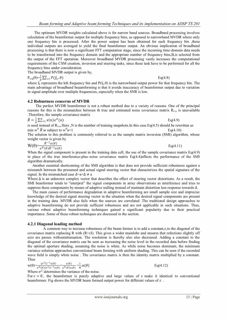
4.2.1 Diagonal loading method A common way to increase robustness of the beam former is to add a constant,𝜀,to the diagonal of the

covariance matrix replacing R with (R+𝜀I). This gives a wider mainlobe and ensures that refections slightly off axis are passes withoutattenuation. The resolution is thereby also also decreased. Adding a constant to the

diagonal of the covariance matrix can be seen as increasing the noise level in the recorded data before finding

the optimal aperture shading, assuming the noise is white. As while noise becomes dominant, the minimum

variance solution approaches conventional beam forming with uniform shading. This can be seen if the recorded

wave field is simply white noise . The covariance matrix is then the identity matrix multiplied by a constant.

Thus

w(θ)=(𝜎2𝐼)−1𝑎(𝜃)

𝑎𝐻 𝜃 (𝜎2𝐼)−1𝑎(𝜃)=

𝑎(𝜃 )

𝑎𝐻 𝜃 𝑎(𝜃) =

1

𝑀𝑎(𝜃) Eq(4.12)

Where 𝜎2 determines the variance of the noise.

For 𝜀 = 0 , the beamformer is purely adaptive and large values of 𝜀 make it identical to conventional

beamformer. Fig shows the MVDR beam formed output power for different values of 𝜀 .



Fig.4.1 MVDR beamformer output power for different values of 𝜺

V. Real Time Implementation In the real time cases of array signal processing, a hardware implementation is required. Here the

implementation is done in ADSP-TS201 processor, a TigerSHARC processor which is a 32-bit, high

performance DSP. The TigerSHARC processor sets a new standard of performance for digital signal processors,

combining multiple computation units for floating-point and fixed-point processing as well as very wide word

widths.

In the hardware implementation procedure, the Matlab code is first converted to C code. For this a

windows based software debugging environment for digital signal processors is used. This environment is

known as Visual DSP++. The C code is then converted to assembly code with the help of this software. Loader

files are then created and loaded into the DSP processor with the help of a serial port communicator.

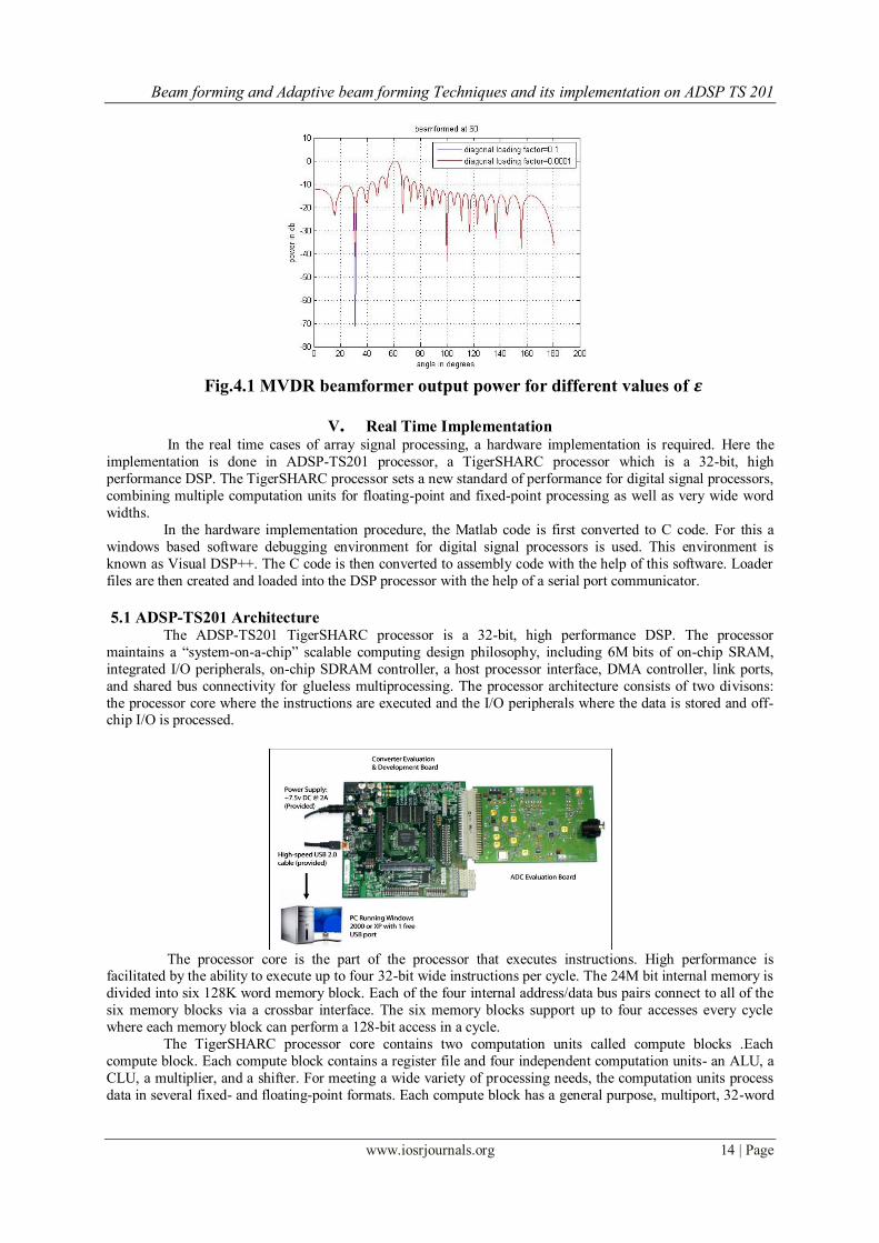
5.1 ADSP-TS201 Architecture The ADSP-TS201 TigerSHARC processor is a 32-bit, high performance DSP. The processor

maintains a “system-on-a-chip” scalable computing design philosophy, including 6M bits of on-chip SRAM,

integrated I/O peripherals, on-chip SDRAM controller, a host processor interface, DMA controller, link ports,

and shared bus connectivity for glueless multiprocessing. The processor architecture consists of two divisons:

the processor core where the instructions are executed and the I/O peripherals where the data is stored and off-chip I/O is processed.

The processor core is the part of the processor that executes instructions. High performance is

facilitated by the ability to execute up to four 32-bit wide instructions per cycle. The 24M bit internal memory is

divided into six 128K word memory block. Each of the four internal address/data bus pairs connect to all of the

six memory blocks via a crossbar interface. The six memory blocks support up to four accesses every cycle

where each memory block can perform a 128-bit access in a cycle.

The TigerSHARC processor core contains two computation units called compute blocks .Each

compute block. Each compute block contains a register file and four independent computation units- an ALU, a

CLU, a multiplier, and a shifter. For meeting a wide variety of processing needs, the computation units process

data in several fixed- and floating-point formats. Each compute block has a general purpose, multiport, 32-word



data register file for transferring data between the computational units and the data buses and storing

intermediate results.

5.1.1 Integer arthimetic logic unit (IALU)

The IALUs can execute standard standalone ALU operations on IALU register files. The IALUs also

execute register load, store, and transfer operations, providing memory addresses when data is transferred

between memory and registers. The processor has dual IALUs that enable simultaneous addresses for two

transactions up to 128 bits in parallel. Each IALU has a multiport, 32-word register file.

5.1.2 Program Sequencer

The program sequencer supplies instruction addresses to memory and, together with the IALUs, allows

compute operations to execute with maximum efficiency. The sequencer supports efficient branching using the

branch target buffer, which reduces branch delays for conditional and unconditional instructions. The two

responsibilities of the sequencer are to decode fetched instructions- separating the instruction slots of the instruction line and sending each instruction to its execution unit and to control the program flow.

5.1.3 Memory, registers, and buses

The on-chip memory consists of six blocks of 4M bits each. Each block is 128K words, thus providing

high bandwidth sufficient to support both computation units, the instruction stream and external I/O, even in

very intensive operations. The memory blocks can store instructions and data interchangeably. Each memory

block is organized as 128K words of 32 bits each. The six memory blocks are a resource that must be shared

between the compute blocks, the IALUs, the sequencer, the external port, and the link ports.

5.1.4 Internal buses

The processor core has three buses, each connected to all of the internal memory blocks via a crossbar

interface. These buses are 128 bits wide to allow up to four instructions, or four aligned data words, to be transferred in each cycle on each bus. On-chip system elements use the SOV bus and S-bus to access memory.

Only one access to each memory block is allowed in each cycle, so if the application accesses a different

memory segment for each purpose, all transactions can be executed with no stalls.

5.1.5 Internal Registers

Most registers of the ADSP-TSP201 processor are classified as universal registers. Instructions are

provided for transferring data between any two U registers, between a u and memory, or for the immediate load

of a u. This includes control registers and status registers, as well as the data registers in the register files.

5.1.6 SOC Interface

The system-on- chip (SOC) interface connects the processor core‟s buses o the I/O peripherals‟ SOC bus. The SOC bus is 128-bits wide, and its clock operates at one half the processor core clock rate. All data transferred

between internal memory or core, and external port passes through this bus.

5.1.7 Timers

The TigerSHARC processor has two general-purpose 64-bit timers- timer0 and timer1. The timers are free

running counters that are loaded with an initial value and give an indication when expiring. The indication is

normally an interrupt, but could also be an external pin for timer0.

5.1.8 Flags

The TigerSHARC processor has four general purpose input or output flag pins. Each pin may be configured as

an input or output. As outputs, programs may use the flag pins to signal events or conditions to any external

device such as a host processor. As inputs, programs may read the flag pin input state in the FLAGREG register

or use the pin input state as a condition in conditional instructions. After power up reset, the FLAG3-0 pins are

inputs with internal pull up resistors that hold them at logic high value.

5.1.9 Interrupts

The ADSP-TS201 processor four general purpose external interrupts, IRQ3-0. The processor also has internally

generated interrupts for the two timers, DMA channels, link ports, arithmetic exceptions, multiprocessor vector

interrupts, and user defined software interrupts. Interrupts can be nested through instruction commands.

Interrupts have a short latency and do not abort currently executing instructions. Interrupt vectors direct to a user

supplied address in the interrupt table register file, removing the overhead of a second branch.

5.10 Direct Memory Access

The TigerSHARC processor on-chip DMA controller relieves the processor core of the burden of moving data

between internal memory and an external device, or between link ports and internal or external memory. The

fully integrated DMA controller allows the the TigerSHARC processor, or an external device to specify data



transfer operations and return to normal processing while the DMA controller carries out the data transfers in the

background. There are 14 channels of which four are dedicated to the transfer of data to and from external

memory devices, eight to the link ports two to the Auto DMA registers.

VI. Comparative Study Of Mvdr And Conventional Beamforming

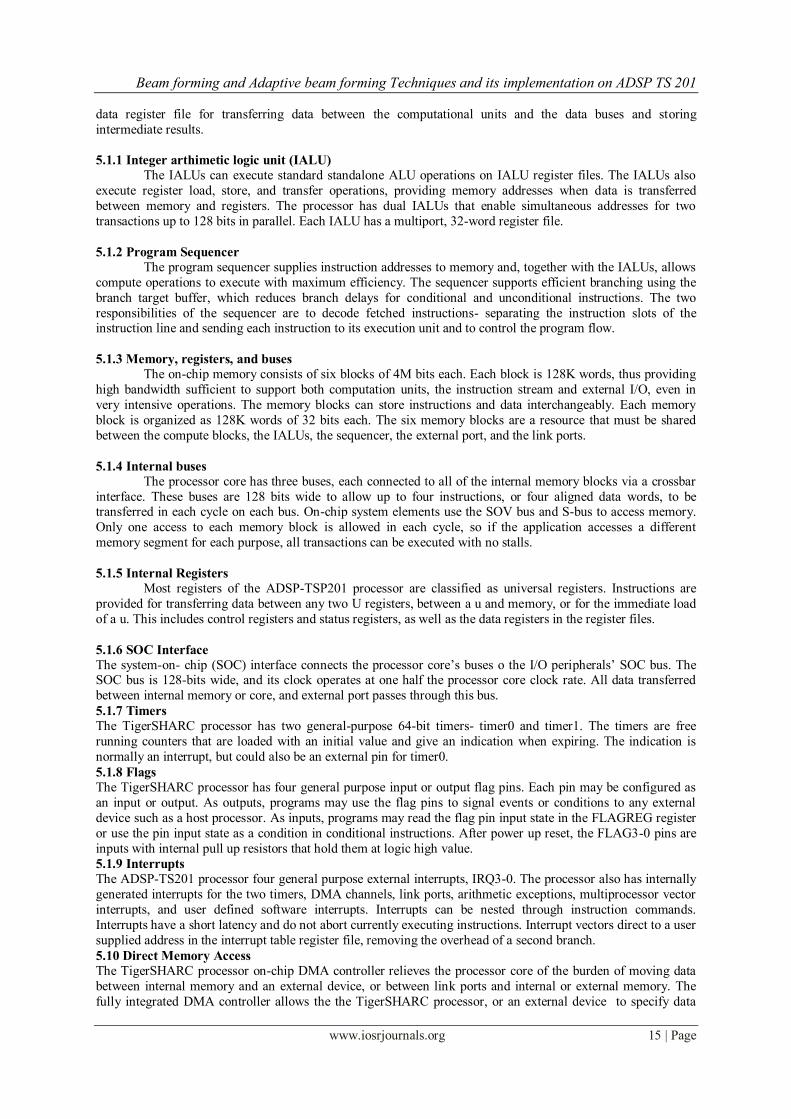
6.1 Beamforming Resolution Array aperture is the finite area over which a sensor collects spatial energy. In the case of ULA, the aperture is the distance between the first and the last elements. In general the greater the aperture, finer the

resolution of the array. Resolution is the ability to distinguish between closely spaced sources. Improved

resolution results in better angle estimation capabilties.

Let us consider two closely spaced targets situated at θ=600 and θ=550 .We plot the beamformer

output for the conventional and MVDR cases .We see that in the case of conventional, as the two targets gets

closer the ability to resolve decreases significantly. Whereas in the case of adaptive beamforming, the resolution

obtained is so high that the ability to distinguish between two targets is very high.

Fig.6.1 MVDR and Conventional beamformer outputs

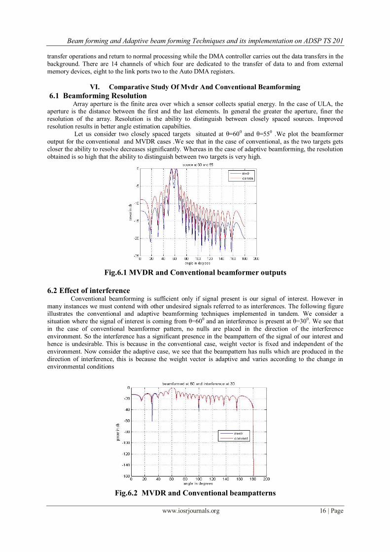
6.2 Effect of interference Conventional beamforming is sufficient only if signal present is our signal of interest. However in

many instances we must contend with other undesired signals referred to as interferences. The following figure illustrates the conventional and adaptive beamforming techniques implemented in tandem. We consider a

situation where the signal of interest is coming from θ=600 and an interference is present at θ=300. We see that

in the case of conventional beamformer pattern, no nulls are placed in the direction of the interference

environment. So the interference has a significant presence in the beampattern of the signal of our interest and

hence is undesirable. This is because in the conventional case, weight vector is fixed and independent of the

environment. Now consider the adaptive case, we see that the beampattern has nulls which are produced in the

direction of interference, this is because the weight vector is adaptive and varies according to the change in

environmental conditions

Fig.6.2 MVDR and Conventional beampatterns



VII. Conclusion Passive arrays use beamforming techniques to detect presence and direction of arrival of underwater

sound sources. One of the simplest non-parametric DOA estimation methods is commonly referred to as the

conventional beamformer. It is based on scanning the array beam and computing the output power for each

beam scan angle. Although the conventional beamformer is rather limited in its angular resolution, its significant

advantages are implementation simplicity and robustness. To overcome the low resolution property of the

conventional beamformer, we estimate the spatial spectrum of multiple sources by means of a spatial filter that

maintains a distortionless response towards the signal coming from the direction „Ɵ‟ while minimizing the total

array output power. Minimum variance distortion less response is an adaptive algorithm which will minimise

the output in all directions subject to the condition that gain in the steering direction is unity. The steering

direction is the bearing that the array is steered towards to look for a particular incoming signal. This algorithm

gives optimum performance by steering nulls in the direction of interference and also offers better performance in the case of correlated noise sources.

References [1] H.L. Van Trees, “Optimum Array Processing - Part IV of Detection, Estimation and Modulation Theory,” John Wiley & Sons Inc.,

New York, 2002.

[2] D. Johnson and D. Dudgeon, “Array Signal Processing Concepts and Techniques,” Prentice Hall, Upper Saddle River, NJ, 1993.

[3] Van Veen, D.,Buckley, M., “Beam forming: A versatile approach to spatial filtering”, IEEE ASSP Magazine, April 1988.

[4] Hamid Krim, Mats Viberg, “Two decades of array signal processing research”, IEEE signal Processing Magazine, July 1996.

[5] www.analog.com/en/embedded.../tigersharc/processors/.../index.html

AUTHORS PROFILE

Prasanth C.R Received Diploma in Electronics and Instrumentation from govt. Polytechnic

cherthala (first class with distinction, Third rank and gold medallist). He passed Btech in

Electronics and Communication Engg from M.G University Kerala placed in first class with

distinction He currently pursing Mtech in Digital signal processing from Govt. Engg college cherthala under Cochin University of science and technology(CUSAT) Kerala India. He

published four research articles in international journals. His areas of research include

digital image processing, statistical signal processing etc

Sreeja K S received the B- tech degree from Rajagiri School of Engineering and

Technology under Mahatma Gandhi University,Kochi,Kerala,India.She is currently doing

M-Tech in Electronics with specialization in Signal Processing in Govt.College of

Engineering Cherthala under Cochin University of Science and Technology,Kerala,India.

Prince Joseph received currently pursig Btech in electronics and communication engineering

from college of engg cherthala under Cochin University of science and technology

Nidheesh. H currently pursig Btech in electronics and communication engineering from

college of engg cherthala under Cochin University of science and technology

beam forming and adaptive beam forming techniques and its...

Documents