30 1. Graph Theory

Small world networks have the property that characteristic path lengths are lowand clustering coef�cients are high. Graphs that have these properties can be usedas models in the mathematical analyses of the small world phenomenon and itsassociated concepts. It is interesting to note that other well known networks haveexhibited small world traits — the internet, electric power grids, and even neuralnetworks are examples — and this increases even further the applicability of graphmodels.

Exercises1. Compute the characteristic path length for each of each of the following

graphs: P2k, P2k+1, C2k , C2k+1, Kn, Km,n.

2. Compute the clustering coef�cient for each of each of the following graphs:P2k, P2k+1, C2k, C2k+1, Kn, Km,n.

3. (a) In the Acquaintance Graph, try to �nd a path from your vertex to thevertex of the President of the United States.

(b) Your path from the previous question may not be your shortest suchpath. Prove that your actual distance from the President is at mostone away from the shortest such distance to be found among yourclassmates.

Interesting Note: There are several contexts in which Bacon numbers can be cal-culuated. While Bacon purists only use movie connections, others include sharedappearances on television and in documentaries as well. Under these more openguidelines, the mathematician Paul Erd�os actually has a Bacon number of 3! Erd�oswas the focus of the 1993 documentary N is a Number [63]. British actor AlecGuinness made a (very) brief appearance near the beginning of that �lm, andGuinness has a Bacon number of 2 (can you �nd the connections?). As far aswe know, Bacon has not coauthored a research article with anyone who is con-nected to Erd�os, and so while Erd�os’ Bacon number is 3, Bacon’s Erd�os numberis in�nity.

1.3 Trees“O look at the trees!” they cried, “O look at the trees!”

— Robert Bridges, London Snow

In this section we will look at the trees—but not the ones that sway in the windor catch the falling snow. We will talk about graph-theoretic trees. Before movingon, glance ahead at Figure 1.30, and try to pick out which graphs are trees.

Textbook Combinatorics and GraphTheoryby Harris Hirst Mossinghoff

1.3 Trees 31

1.3.1 De�nitions and ExamplesExample, the surest method of instruction.

— Pliny the Younger

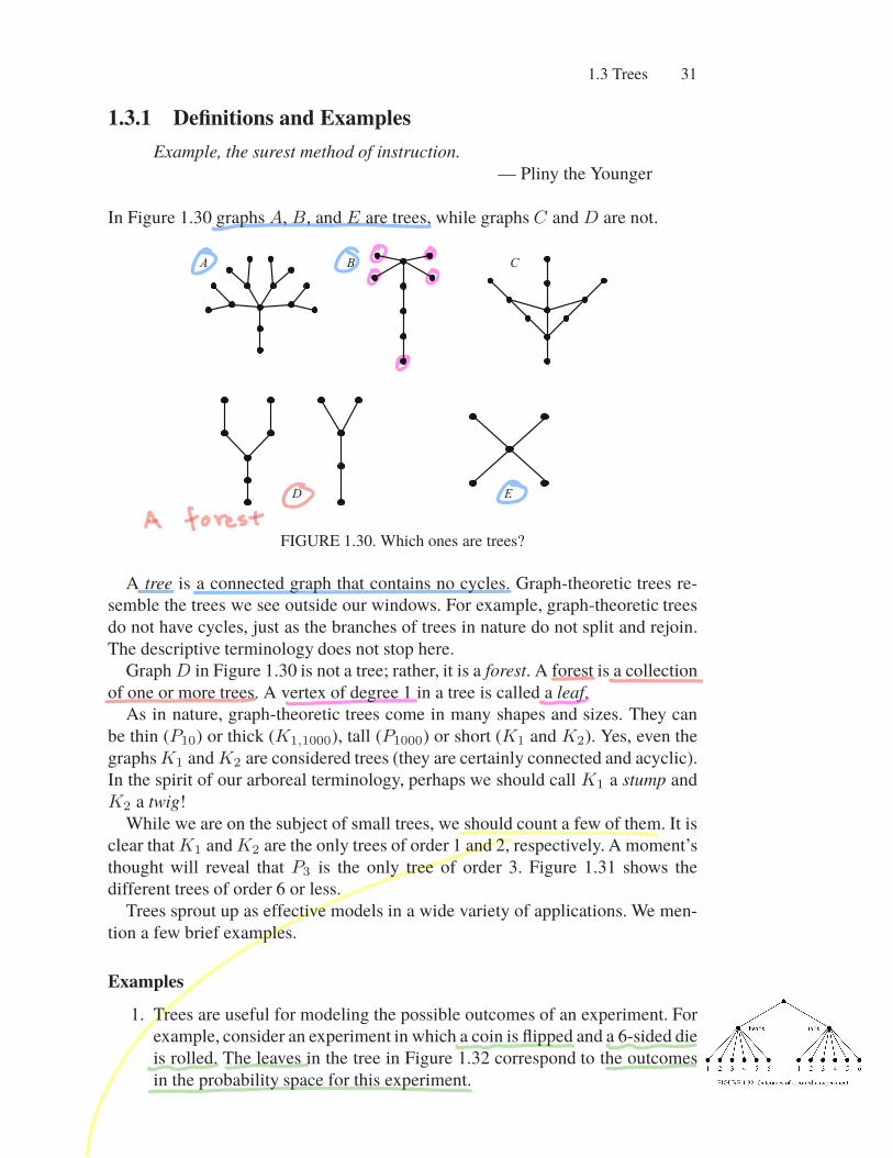
In Figure 1.30 graphs A, B, and E are trees, while graphs C and D are not.

�

! "

FIGURE 1.30. Which ones are trees?

A tree is a connected graph that contains no cycles. Graph-theoretic trees re-semble the trees we see outside our windows. For example, graph-theoretic treesdo not have cycles, just as the branches of trees in nature do not split and rejoin.The descriptive terminology does not stop here.

Graph D in Figure 1.30 is not a tree; rather, it is a forest. A forest is a collectionof one or more trees. A vertex of degree 1 in a tree is called a leaf.

As in nature, graph-theoretic trees come in many shapes and sizes. They canbe thin (P10) or thick (K1,1000), tall (P1000) or short (K1 and K2). Yes, even thegraphs K1 and K2 are considered trees (they are certainly connected and acyclic).In the spirit of our arboreal terminology, perhaps we should call K1 a stump andK2 a twig!

While we are on the subject of small trees, we should count a few of them. It isclear that K1 and K2 are the only trees of order 1 and 2, respectively. A moment’sthought will reveal that P3 is the only tree of order 3. Figure 1.31 shows thedifferent trees of order 6 or less.

Trees sprout up as effective models in a wide variety of applications. We men-tion a few brief examples.

Examples1. Trees are useful for modeling the possible outcomes of an experiment. For

example, consider an experiment in which a coin is �ipped and a 6-sided dieis rolled. The leaves in the tree in Figure 1.32 correspond to the outcomesin the probability space for this experiment.

32 1. Graph Theory

�

�

�

� �

FIGURE 1.31. Trees of order 6 or less.

� � � � � � � � � �

����� �����

FIGURE 1.32. Outcomes of a coin/die experiment.

2. Programmers often use tree structures to facilitate searches and sorts andto model the logic of algorithms. For instance, the logic for a program that�nds the maximum of four numbers (w, x, y, z) can be represented by thetree shown in Figure 1.33. This type of tree is a binary decision tree.

3. Chemists can use trees to represent, among other things, saturated hydro-carbons—chemical compounds of the form CnH2n+2 (propane, for exam-ple). The bonds between the carbon and hydrogen atoms are depicted in thetrees of Figure 1.34. The vertices of degree 4 are the carbon atoms, and theleaves represent the hydrogen atoms.

4. College basketball fans will recognize the tree in Figure 1.35. It displays�nal results for the “Sweet 16” portion of the 2008 NCAA men’s basketballtournament. Each vertex represents a single game.

1.3 Trees 33

����������

����������

����������

����������

����������

����������

����������

����������

�� �

�� ��� � �� � �� �

�� ��� �

� �

� � � �

� � � � � � � �

FIGURE 1.33. Logic of a program.

������ ������� �������

FIGURE 1.34. A few saturated hydrocarbons.

�!���

"���#���

$�%

&�����"��

'�(��!����

)��������

*�����

+������!�

&��,�����

-�!�����

*�����

-�!�����

$�%

'�(��!����

$�%

*�����

.������

.�,���"��

)����

$%'/

&��*���(,01

&��+��2����

.������

)����

$%'/

�!���

.������

$%'/

.������

*�����

FIGURE 1.35. The 2008 Men’s Sweet 16.

Exercises1. Draw all unlabeled trees of order 7. Hint: There are a prime number of

them.

2. Draw all unlabeled forests of order 6.

3. Let T be a tree of order n � 2. Prove that T is bipartite.

Sec L 3.1 Definitions and Examples

34 1. Graph Theory

4. Graphs of the form K1,n are called stars. Prove that if Kr,s is a tree, then itmust be a star.

5. Match the graphs in Figure 1.36 with appropriate names: a palm tree, au-tumn, a path through a forest, tea leaves.

�

!

"

FIGURE 1.36. What would you name these graphs?

1.3.2 Properties of TreesAnd the tree was happy.

— Shel Silverstein, The Giving Tree

Let us try an experiment. On a piece of scratch paper, draw a tree of order 16.Got one? Now count the number of edges in the tree. We are going to go out ona limb here and predict that there are 15. Since there are nearly 20,000 differenttrees of order 16, it may seem surprising that our prediction was correct. The nexttheorem gives away our secret.

Theorem 1.10. If T is a tree of order n, then T has n � 1 edges.

Proof. We induct on the order of T . For n = 1 the only tree is the stump (K1),and it of course has 0 edges. Assume that the result is true for all trees of orderless than k, and let T be a tree of order k.

Choose some edge of T and call it e. Since T is a tree, it must be that T � eis disconnected (see Exercise 7) with two connected components that are treesthemselves (see Figure 1.37). Say that these two components of T � e are T1

and T2, with orders k1 and k2, respectively. Thus, k1 and k2 are less than n andk1 + k2 = k.

Since k1 < k, the theorem is true for T1. Thus T1 has k1 � 1 edges. Similarly,T2 has k2 � 1 edges. Now, since E(T ) is the disjoint union of E(T1), E(T2), and{e}, we have |E(T )| = (k1 � 1) + (k2 � 1) + 1 = k1 + k2 � 1 = k � 1. Thiscompletes the induction.

I 2 34 567 8 910 11 12

13 14 15

16

rpg38

K

1.3 Trees 35

�#� #�

FIGURE 1.37.

The next theorem extends the preceding result to forests. The proof is similarand appears as Exercise 4.

Theorem 1.11. If F is a forest of order n containing k connected components,then F contains n � k edges.

The next two theorems give alternative methods for de�ning trees. Two othermethods are given in Exercises 5 and 6.

Theorem 1.12. A graph of order n is a tree if and only if it is connected andcontains n � 1 edges.

Proof. The forward direction of this theorem is immediate from the de�nition oftrees and Theorem 1.10. For the reverse direction, suppose a graph G of ordern is connected and contains n � 1 edges. We need to show that G is acyclic. IfG did have a cycle, we could remove an edge from the cycle and the resultinggraph would still be connected. In fact, we could keep removing edges (one ata time) from existing cycles, each time maintaining connectivity. The resultinggraph would be connected and acyclic and would thus be a tree. But this treewould have fewer than n � 1 edges, and this is impossible by Theorem 1.10.Therefore, G has no cycles, so G is a tree.

Theorem 1.13. A graph of order n is a tree if and only if it is acyclic and containsn � 1 edges.

Proof. Again the forward direction of this theorem follows from the de�nition oftrees and from Theorem 1.10. So suppose that G is acyclic and has n � 1 edges.To show that G is a tree we need to show only that it is connected. Let us say thatthe connected components of G are G1, G2, . . . , Gk. Since G is acyclic, each ofthese components is a tree, and so G is a forest. Theorem 1.11 tells us that G hasn � k edges, implying that k = 1. Thus G has only one connected component,implying that G is a tree.

It is not uncommon to look out a window and see lea�ess trees. In graph theory,though, lea�ess trees are rare indeed. In fact, the stump (K1) is the only such tree,and every other tree has at least two leaves. Take note of the proof technique ofthe following theorem. It is a standard graph theory induction argument.

Theorem 1.14. Let T be the tree of order n � 2. Then T has at least two leaves.

Proof. Again we induct on the order. The result is certainly true if n = 2, sinceT = K2 in this case. Suppose the result is true for all orders from 2 to n� 1, andconsider a tree T of order n � 3. We know that T has n � 1 edges, and sincewe can assume n � 3, T has at least 2 edges. If every edge of T is incident with

I

36 1. Graph Theory

a leaf, then T has at least two leaves, and the proof is complete. So assume thatthere is some edge of T that is not incident with a leaf, and let us say that this edgeis e = uv. The graph T � e is a pair of trees, T1 and T2, each of order less than n.Let us say, without loss of generality, that u � V (T1), v � V (T2), |V (T1)| = n1,and |V (T2)| = n2 (see Figure 1.38). Since e is not incident with any leaves of T ,

#� #�

$ �

FIGURE 1.38.

we know that n1 and n2 are both at least 2, so the induction hypothesis applies toeach of T1 and T2. Thus, each of T1 and T2 has two leaves. This means that eachof T1 and T2 has at least one leaf that is not incident with the edge e. Thus thegraph (T � e) + e = T has at least two leaves.

We saw in the previous section that the center of a graph is the set of verticeswith minimum eccentricity. The next theorem, due to Jordan [170], shows that fortrees, there are only two possibilities for the center.

Theorem 1.15. In any tree, the center is either a single vertex or a pair of adja-cent vertices.

Proof. Given a tree T , we form a sequence of trees as follows. Let T0 = T . LetT1 be the graph obtained from T0 by deleting all of its leaves. Note here that T1

is also a tree. Let T2 be the tree obtained from T1 by deleting all of the leaves ofT1. In general, for as long as it is possible, let Tj be the tree obtained by deletingall of the leaves of Tj�1. Since T is �nite, there must be an integer r such that Tr

is either K1 or K2.Consider now a consecutive pair Ti, Ti+1 of trees from the sequence T = T0,

T1, . . . , Tr. Let v be a non-leaf of Ti. In Ti, the vertices that are at the greatestdistance from v are leaves (of Ti). This means that the eccentricity of v in Ti+1 isone less than the eccentricity of v in Ti. Since this is true for all non-leaves of Ti,it must be that the center of Ti+1 is exactly the same as the center of Ti.

Therefore, the center of Tr is the center of Tr�1, which is the center of Tr�2,. . . , which is the center of T0 = T . Since (the center of) Tr is either K1 or K2,the proof is complete.

We conclude this section with an interesting result about trees as subgraphs.

Theorem 1.16. Let T be a tree with k edges. If G is a graph whose minimumdegree satis�es �(G) � k, then G contains T as a subgraph. Alternatively, Gcontains every tree of order at most �(G) + 1 as a subgraph.

Skip

1.3 Trees 37

Proof. We induct on k. If k = 0, then T = K1, and it is clear that K1 is asubgraph of any graph. Further, if k = 1, then T = K2, and K2 is a subgraph ofany graph whose minimum degree is 1. Assume that the result is true for all treeswith k � 1 edges (k � 2), and consider a tree T with exactly k edges. We knowfrom Theorem 1.14 that T contains at least two leaves. Let v be one of them, andlet w be the vertex that is adjacent to v. Consider the graph T � v. Since T � v

#%�

�$

FIGURE 1.39.

has k � 1 edges, the induction hypothesis applies, so T � v is a subgraph of G.We can think of T � v as actually sitting inside of G (meaning w is a vertex of G,too). Now, since G contains at least k + 1 vertices and T � v contains k vertices,there exist vertices of G that are not a part of the subgraph T � v. Further, sincethe degree in G of w is at least k, there must be a vertex u not in T � v that isadjacent to w (Figure 1.40). The subgraph T � v together with u forms the tree T

#%�

�$

FIGURE 1.40. A copy of T inside G.

as a subgraph of G.

Exercises1. Draw each of the following, if you can. If you cannot, explain the reason.

(a) A 10-vertex forest with exactly 12 edges(b) A 12-vertex forest with exactly 10 edges(c) A 14-vertex forest with exactly 14 edges(d) A 14-vertex forest with exactly 13 edges(e) A 14-vertex forest with exactly 12 edges

2. Suppose a tree T has an even number of edges. Show that at least one vertexmust have even degree.

3. Let T be a tree with max degree �. Prove that T has at least � leaves.

Skip

O

38 1. Graph Theory

4. Let F be a forest of order n containing k connected components. Prove thatF contains n � k edges.

5. Prove that a graph G is a tree if and only if for every pair of vertices u, v,there is exactly one path from u to v.

6. Prove that T is a tree if and only if T contains no cycles, and for any newedge e, the graph T + e has exactly one cycle.

7. Show that every edge in a tree is a bridge.

8. Show that every nonleaf in a tree is a cut vertex.

9. Find a shorter proof to Theorem 1.14. Hint: Start by considering a longestpath in T .

10. Let T be a tree of order n > 1. Show that the number of leaves is

2 +

deg(vi)�3

(deg(vi) � 2),

where the sum is over all vertices of degree 3 or more.

11. For a graph G, de�ne the average degree of G to be

avgdeg(G) =

�v�V (G) deg(v)|V (G)| .

If T is a tree and avgdeg(T ) = a, then �nd an expression for the numberof vertices in T in terms of a.

12. Let T be a tree such that every vertex adjacent to a leaf has degree at least3. Prove that some pair of leaves in T has a common neighbor.

1.3.3 Spanning TreesUnder the spreading chestnut tree . . .

— Henry W. Longfellow, The Village Blacksmith

The North Carolina Department of Transportation (NCDOT) has decided to im-plement a rapid rail system to serve eight cities in the western part of the state.Some of the cities are currently joined by roads or highways, and the state plansto lay the track right along these roads. Due to the mountainous terrain, some ofthe roads are steep and curvy; and so laying track along these roads would bedif�cult and expensive. The NCDOT hired a consultant to study the roads and toassign dif�culty ratings to each one. The rating accounted for length, grade, andcurviness of the roads; and higher ratings correspond to greater cost. The graph

1.3 Trees 39

�3

��

�3��

4��3

3�3

��

�3

�3

5�##�����6����

6������7�0

'��!����

.����� 8�,0��1

'�����

6��9��2�:�,0

FIGURE 1.41. The city graph.

in Figure 1.41, call it the “city graph,” shows the result of the consultant’s inves-tigation. The number on each edge represents the dif�culty rating assigned to theexisting road.

The state wants to be able to make each city accessible (but not necessarilydirectly accessible) from every other city. One obvious way to do this is to laytrack along every one of the existing roads. But the state wants to minimize cost,so this solution is certainly not the best, since it would result in a large amountof unnecessary track. In fact, the best solution will not include a cycle of trackanywhere, since a cycle would mean at least one segment of wasted track.

The situation above motivates a de�nition. Given a graph G and a subgraph T ,we say that T is a spanning tree of G if T is a tree that contains every vertex ofG.

So it looks as though the DOT just needs to �nd a spanning tree of the citygraph, and they would like to �nd one whose overall rating is as small as possible.Figure 1.42 shows several attempts at a solution.

Of the solutions in the �gure, the one in the upper right has the least totalweight—but is it the best one overall? Try to �nd a better one. We will come backto this problem soon.

Given a graph G, a weight function is a function W that maps the edges ofG to the nonnegative real numbers. The graph G together with a weight func-tion is called a weighted graph . The graph in Figure 1.41 is a simple example ofa weighted graph. Although one might encounter situations where negative val-ued weights would be appropriate, we will stick with nonnegative weights in ourdiscussion.

It should be fairly clear that every connected graph has at least one spanningtree. In fact, it is not uncommon for a graph to have many different spanning trees.Figure 1.42 displays three different spanning trees of the city graph.

Given a connected, weighted graph G, a spanning tree T is called a minimumweight spanning tree if the sum of the weights of the edges of T is no more thanthe sum for any other spanning tree of G.

ofthecitygraph

40 1. Graph Theory

)�����&��2���;��43

)�����&��2���;����

�3

���3

4��3

3�3

�3

����

4��3

3�3

�3

���3

�3

3

��

�3

)�����&��2���;���3

FIGURE 1.42. Several spanning trees.

There are a number of fairly simple algorithms for �nding minimum weightspanning trees. Perhaps the best known is Kruskal’s algorithm.

Kruskal’s Algorithm

Given: A connected, weighted graph G.

i. Find an edge of minimum weight and mark it.

ii. Among all of the unmarked edges that do not form a cycle with any of themarked edges, choose an edge of minimum weight and mark it.

iii. If the set of marked edges forms a spanning tree of G, then stop. If not,repeat step ii.

Figure 1.43 demonstrates Kruskal’s algorithm applied to the city graph. Theminimum weight is 210.

It is certainly possible for different trees to result from two different appli-cations of Kruskal’s algorithm. For instance, in the second step we could havechosen the edge between Marion and Lenoir instead of the one that was chosen.Even so, the total weight of resulting trees is the same, and each such tree is aminimum weight spanning tree.

1.3 Trees 41

)<)/'�&7=>8)?����3�3

�3

���3��

4��3

3�3

��

�3

�3

�3

���3��

4��3

3�3

��

�3

�3

�3

���3��

4��3

3�3

��

�3

�3

�3

���3��

4��3

3�3

��

�3

�3

�3

���3��

4��3

3�3

��

�3

�3

���3��

4��3

3�3

��

�3

�3

���3��

4��3

3�3

��

�3 �3

�3

FIGURE 1.43. The stages of Kruskal’s algorithm.

It should be clear from the algorithm itself that the subgraph built is in facta spanning tree of G. How can we be sure, though, that it has minimum totalweight? The following theorem answers our question [183].

Theorem 1.17. Kruskal’s algorithm produces a spanning tree of minimum totalweight.

Proof. Let G be a connected, weighted graph of order n, and let T be a spanningtree obtained by applying Kruskal’s algorithm to G. As we have seen, Kruskal’salgorithm builds spanning trees by adding one edge at a time until a tree is formed.Let us say that the edges added for T were (in order) e1, e2, . . . , en�1. SupposeT is not a minimum weight spanning tree. Among all minimum weight spanningtrees of G, choose T � to be a minimum weight spanning tree that agrees withthe construction of T for the longest time (i.e., for the most initial steps). This

Note This is an example of a greedy algorithm

42 1. Graph Theory

means that there exists some k such that T � contains e1, . . . , ek, and no minimumweight spanning tree contains all of e1, . . . , ek, ek+1 (notice that since T is not ofminimum weight, k < n � 1).

Since T � is a spanning tree, it must be that T � + ek+1 contains a cycle C, andsince T contains no cycles, C must contain some edge, say e�, that is not in T .If we remove the edge e� from T � + ek+1, then the cycle C is broken and whatremains is a spanning tree of G. Thus, T � + ek+1 � e� is a spanning tree of G, andit contains edges e1, . . . , ek, ek+1. Furthermore, since the edge e� must have beenavailable to be chosen when ek+1 was chosen by the algorithm, it must be thatw(ek+1) � w(e�). This means that T � + ek+1 � e� is a spanning tree with weightno more than T � that contains edges e1, . . . , ek+1, contradicting our assumptions.Therefore, it must be that T is a minimum weight spanning tree.

Exercises1. Prove that every connected graph contains at least one spanning tree.

2. Prove that a graph is a tree if and only if it is connected and has exactly onespanning tree.

3. Let G be a connected graph with n vertices and at least n edges. Let C be acycle of G. Prove that if T is a spanning tree of G, then T , the complementof T , contains at least one edge of C.

4. Let G be connected, and let e be an edge of G. Prove that e is a bridge ifand only if it is in every spanning tree of G.

5. Using Kruskal’s algorithm, �nd a minimum weight spanning tree of thegraphs in Figure 1.44. In each case, determine (with proof) whether theminimum weight spanning tree is unique.

�

��

��

�

� ��

�

�

��

�3

��

4

�

�

�

FIGURE 1.44. Two weighted graphs.

Sec 1 3.3 Spanning Trees

0

a D

1.3 Trees 43

6. Prim’s algorithm (from [228]) provides another method for �nding mini-mum weight spanning trees.

Prim’s Algorithm

Given: A connected, weighted graph G.

i. Choose a vertex v, and mark it.ii. From among all edges that have one marked end vertex and one un-

marked end vertex, choose an edge e of minimum weight. Mark theedge e, and also mark its unmarked end vertex.

iii. If every vertex of G is marked, then the set of marked edges forms aminimum weight spanning tree. If not, repeat step ii.

Use Prim’s algorithm to �nd minimum weight spanning trees for the graphsin Figure 1.44. As you work, compare the stages to those of Kruskal’s al-gorithm.

7. Give an example of a connected, weighted graph G having (i) a cycle withtwo identical weights, which is neither the smallest nor the largest weight inthe graph, and (ii) a unique minimum weight spanning tree which containsexactly one of these two identical weights.

1.3.4 Counting TreesAs for everything else, so for a mathematical theory: beauty can beperceived but not explained.

— Arthur Cayley [214]

In this section we discuss two beautiful results on counting the number of span-ning trees in a graph. The next chapter studies general techniques for countingarrangements of objects, so these results are a sneak preview.

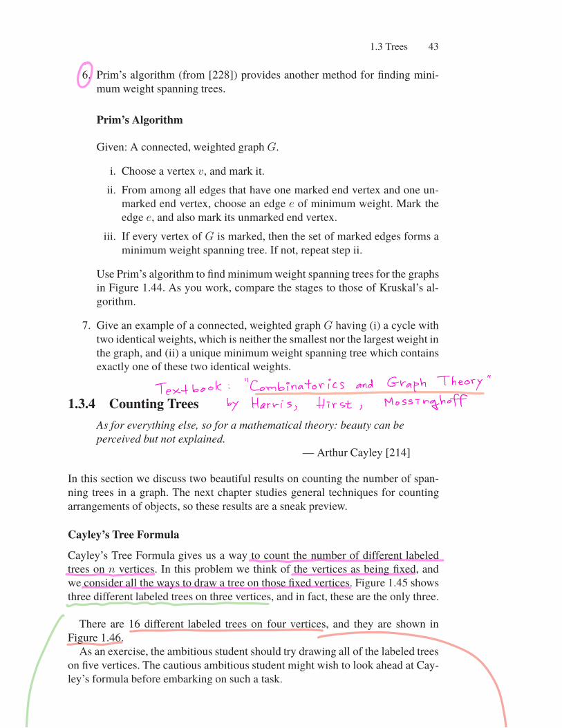
Cayley’s Tree FormulaCayley’s Tree Formula gives us a way to count the number of different labeledtrees on n vertices. In this problem we think of the vertices as being �xed, andwe consider all the ways to draw a tree on those �xed vertices. Figure 1.45 showsthree different labeled trees on three vertices, and in fact, these are the only three.

There are 16 different labeled trees on four vertices, and they are shown inFigure 1.46.

As an exercise, the ambitious student should try drawing all of the labeled treeson �ve vertices. The cautious ambitious student might wish to look ahead at Cay-ley’s formula before embarking on such a task.

Textbook Combinatorics and GraphTheoryby Harris Hirst Mossinghoff

44 1. Graph Theory

�

� �

�

� �

�

� �

FIGURE 1.45. Labeled trees on three vertices.

� �

� �

� �

� �

� �

� �

� �

� �

� �

� �

� �

� �

� �

� �

� �

� �

� �

� �

� �

� �

� �

� �

� �

� �

� �

� �

� �

� �

� �

� �

� �

� �

FIGURE 1.46. Labeled trees on four vertices.

Cayley proved the following theorem in 1889 [50]. The proof technique that wewill describe here is due to Prufer7 [229]. Prufer’s method is almost as noteworthyas the result itself. He counted the labeled trees by placing them in one-to-one cor-respondence with a set whose size is easy to determine—the set of all sequencesof length n� 2 whose entries come from the set {1, . . . , n}. There are nn�2 suchsequences.

Theorem 1.18 (Cayley’s Tree Formula). There are nn�2 distinct labeled trees oforder n.

The algorithm below gives the steps that Prufer used to assign a particular se-quence to a given tree, T , whose vertices are labeled 1, . . . , n. Each labeled treeis assigned a unique sequence.

7With a name like that he was destined for mathematical greatness!

1.3 Trees 45

Prufer’s Method for Assigning a Sequence to a Labeled Tree

Given: A tree T , with vertices labeled 1, . . . , n.

1. Let i = 0, and let T0 = T .

2. Find the leaf on Ti with the smallest label and call it v.

3. Record in the sequence the label of v’s neighbor.

4. Remove v from Ti to create a new tree Ti+1.

5. If Ti+1 = K2, then stop. Otherwise, increment i by 1 and go back to step2.

Let us run through this algorithm with a particular graph. In Figure 1.47, treeT = T0 has 7 vertices, labeled as shown. The �rst step is �nding the leaf withsmallest label: This would be 2. The neighbor of vertex 2 is the vertex labeled4. Therefore, 4 is the �rst entry in the sequence. Removing vertex 2 producestree T1. The leaf with smallest label in T1 is 4, and its neighbor is 3. Therefore,we put 3 in the sequence and delete 4 from T1. Vertex 5 is the smallest leaf intree T2 = T1 � {4}, and its neighbor is 1. So our sequence so far is 4, 3, 1. InT3 = T2�{5} the smallest leaf is vertex 6, whose neighbor is 3. In T4 = T3�{6},the smallest leaf is vertex 3, whose neighbor is 1. Since T5 = K2, we stop here.Our resulting sequence is 4, 3, 1, 3, 1.

Notice that in the previous example, none of the leaves of the original tree Tappears in the sequence. More generally, each vertex v appears in the sequenceexactly deg(v) � 1 times. This is not a coincidence (see Exercise 1). We nowpresent Prufer’s algorithm for assigning trees to sequences. Each sequence getsassigned a unique tree.

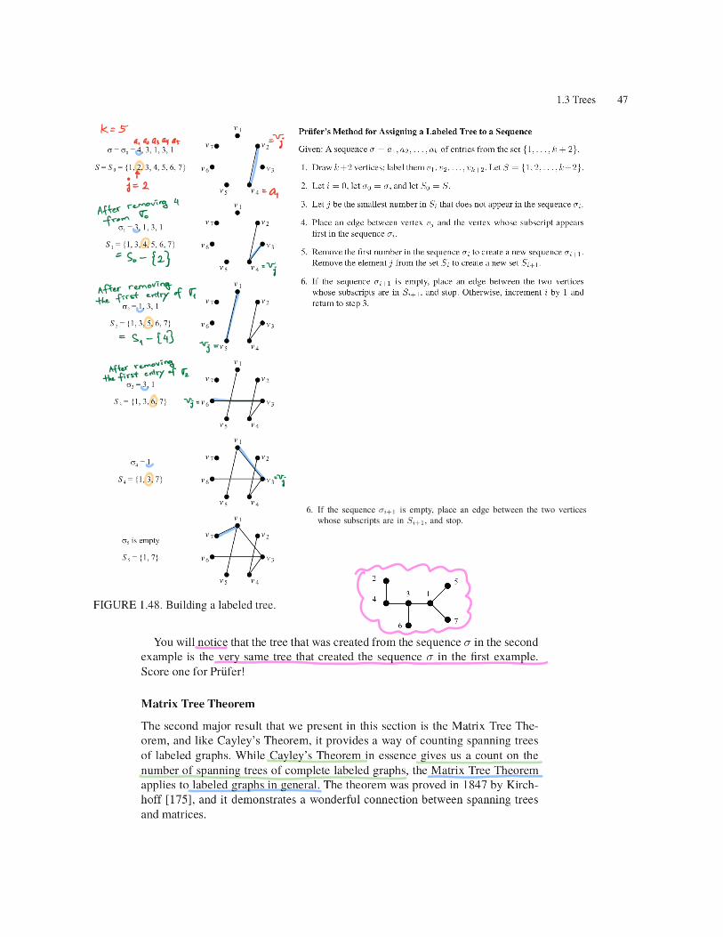
Prufer’s Method for Assigning a Labeled Tree to a Sequence

Given: A sequence � = a1, a2, . . . , ak of entries from the set {1, . . . , k + 2}.

1. Draw k+2 vertices; label them v1, v2, . . . , vk+2. Let S = {1, 2, . . . , k+2}.

2. Let i = 0, let �0 = �, and let S0 = S.

3. Let j be the smallest number in Si that does not appear in the sequence �i.

4. Place an edge between vertex vj and the vertex whose subscript appears�rst in the sequence �i.

5. Remove the �rst number in the sequence �i to create a new sequence �i+1.Remove the element j from the set Si to create a new set Si+1.

6. If the sequence �i+1 is empty, place an edge between the two verticeswhose subscripts are in Si+1, and stop. Otherwise, increment i by 1 andreturn to step 3.

Seenext

j

Seey 47

fi

46 1. Graph Theory

#��

#�� �

#�� �

#�� �

�

#� �� �

�

�

�� �

�

#& #3

7!��!��2�"�@(��,�

�

����

�������������

����������

�������

FIGURE 1.47. Creating a Prufer sequence.

Let us apply this algorithm to a particular example. Let � = 4, 3, 1, 3, 1 beour initial sequence to which we wish to assign a particular labeled tree. Sincethere are �ve terms in the sequence, our labels will come from the set S ={1, 2, 3, 4, 5, 6, 7}. After drawing the seven vertices, we look in the set S = S0

to �nd the smallest subscript that does not appear in the sequence � = �0. Sub-script 2 is the one, and so we place an edge between vertices v2 and v4, the �rstsubscript in the sequence. We now remove the �rst term from the sequence andthe label v2 from the set, forming a new sequence �1 = 3, 1, 3, 1 and a newset S1 = {1, 3, 4, 5, 6, 7}. The remaining steps in the process are shown in Fig-ure 1.48.

theneighbor ofvertex4New tree to

T 43Izthe 2neighbor ofvertex 5

Newtree to

Tz Tz 53 theneighborofvertex6

New tree t14 13 63 the

neighborofvertex 3new tree to15 14 33

Since 75Kz

we stop

44 1. Graph Theory

�

� �

�

� �

�

� �

FIGURE 1.45. Labeled trees on three vertices.

� �

� �

� �

� �

� �

� �

� �

� �

� �

� �

� �

� �

� �

� �

� �

� �

� �

� �

� �

� �

� �

� �

� �

� �

� �

� �

� �

� �

� �

� �

� �

� �

FIGURE 1.46. Labeled trees on four vertices.

Cayley proved the following theorem in 1889 [50]. The proof technique that wewill describe here is due to Prufer7 [229]. Prufer’s method is almost as noteworthyas the result itself. He counted the labeled trees by placing them in one-to-one cor-respondence with a set whose size is easy to determine—the set of all sequencesof length n� 2 whose entries come from the set {1, . . . , n}. There are nn�2 suchsequences.

Theorem 1.18 (Cayley’s Tree Formula). There are nn�2 distinct labeled trees oforder n.

The algorithm below gives the steps that Prufer used to assign a particular se-quence to a given tree, T , whose vertices are labeled 1, . . . , n. Each labeled treeis assigned a unique sequence.

7With a name like that he was destined for mathematical greatness!

Examples of computing Priifer sequenceapp pftTMd

Tree T

b e a Priuiffersequence

ca a ab

I E Ic da ad ab

ta db de ca

aa bb old cc

2

1 5a aasayas TjP8 2 a

Afterremoving4from a

so 2 vjAfterremovingthefirstentryofq

s 43 rjAfterremovingthefirstentryofq

vj

ay

48 1. Graph Theory

The theorem involves two special matrices. One is the adjacency matrix (de-�ned back in Section 1.2.2), and the other is de�ned as follows. Let G be a graphwith vertices v1, v2, . . . vn. The degree matrix of G is the n × n matrix D whose(i, j) entry, denoted by [D]i,j , is de�ned by

[D]i,j =�

deg(vi) if i = j,0 otherwise.

So, the diagonal entries of D are the vertex degrees, and the off-diagonal entriesare all zero.

Given an n × n matrix M , the i, j cofactor of M is de�ned to be(�1)i+j det(M(i|j)),

where det(M(i|j)) represents the determinant of the (n � 1) × (n � 1) matrixformed by deleting row i and column j from M .

We are now ready to state the Matrix Tree Theorem, due to Kirchhoff. Theproof that we give imitates those presented in [148] and [52].Theorem 1.19 (Matrix Tree Theorem). If G is a connected labeled graph withadjacency matrix A and degree matrix D, then the number of unique spanningtrees of G is equal to the value of any cofactor of the matrix D � A.

Proof. Suppose G has n vertices (v1, . . . , vn) and k edges (f1, . . . , fk). Since Gis connected, we know that k is at least n � 1. Let N be the n × k matrix whose(i, j) entry is de�ned by

[N ]i,j =�

1 if vi and fj are incident,0 otherwise.

N is called the incidence matrix of G. Since every edge of G is incident withexactly two vertices of G, each column of N contains two 1’s and n � 2 zeros.Let M be the n × k matrix that results from changing the topmost 1 in eachcolumn to �1. To prove the result, we �rst need to establish two facts, which wecall Claim A and Claim B.

Claim A. MMT = D � A (where MT denotes the transpose of M ).First, notice that the (i, j) entry of D � A is

[D � A]i,j =

�

�

deg(vi) if i = j,�1 if i �= j and vivj � E(G),0 if i �= j and vivj �� E(G).

Now, what about the (i, j) entry of MMT ? The rules of matrix multiplication tellus that this entry is the dot product of row i of M and column j of MT . That is,[MMT ]i,j = ([M ]i,1, [M ]i,2, . . . , [M ]i,k) ·

�[MT ]1,j , [MT ]2,j , . . . , [MT ]k,j

�

= ([M ]i,1, [M ]i,2, . . . , [M ]i,k) · ([M ]j,1, [M ]j,2, . . . , [M ]j,k)

=k

r=1

[M ]i,r[M ]j,r.

D def degGdg

MciIj iffISkipt

1.3 Trees 49

If i = j, then this sum counts one for every nonzero entry in row i; that is, itcounts the degree of vi. If i �= j and vivj �� E(G), then there is no column of Min which both the row i and row j entries are nonzero. Hence the value of the sumin this case is 0. If i �= j and vivj � E(G), then the only column in which boththe row i and the row j entries are nonzero is the column that represents the edgevivj . Since one of these entries is 1 and the other is �1, the value of the sum is�1. We have shown that the (i, j) entry of MMT is the same as the (i, j) entryof D � A, and thus Claim A is proved.

Let H be a subgraph of G with n vertices and n�1 edges. Let p be an arbitraryinteger between 1 and n, and let M � be the (n � 1) × (n � 1) submatrix of Mformed by all rows of M except row p and the columns that correspond to theedges in H .

Claim B. If H is a tree, then | det(M �)| = 1. Otherwise, det(M �) = 0.

First suppose that H is not a tree. Since H has n vertices and n�1 edges, we knowfrom earlier work that H must be disconnected. Let H1 be a connected componentof H that does not contain the vertex vp. Let M �� be the |V (H1)| × (n � 1)submatrix of M � formed by eliminating all rows other than the ones correspondingto vertices of H1. Each column of M �� contains exactly two nonzero entries: 1 and�1. Therefore, the sum of all of the row vectors of M �� is the zero vector, so therows of M �� are linearly dependent. Since these rows are also rows of M �, we seethat det(M �) = 0.

Now suppose that H is a tree. Choose some leaf of H that is not vp (Theo-rem 1.14 lets us know that we can do this), and call it u1. Let us also say that e1 isthe edge of H that is incident with u1. In the tree H � u1, choose u2 to be someleaf other than vp. Let e2 be the edge of H � u1 incident with u2. Keep removingleaves in this fashion until vp is the only vertex left. Having established the list ofvertices u1, u2, . . . , un�1, we now create a new (n� 1)× (n� 1) matrix M� byrearranging the rows of M � in the following way: row i of M� will be the row ofM � that corresponds to the vertex ui.

An important (i.e., useful!) property of the matrix M� is that it is lower tri-angular (we know this because for each i, vertex ui is not incident with any ofei+1, ei+2, . . . , en�1). Thus, the determinant of M� is equal to the product of themain diagonal entries, which are either 1 or �1, since every ui is incident with ei.Thus, | det(M�)| = 1, and so | det(M �)| = 1. This proves Claim B.

We are now ready to investigate the cofactors of D � A = MMT . It is afact from matrix theory that if the row sums and column sums of a matrix are all0, then the cofactors all have the same value. (It would be a nice exercise—and anice review of matrix skills—for you to try to prove this.) Since the matrix MMT

satis�es this condition, we need to consider only one of its cofactors. We mightas well choose i and j such that i + j is even—let us choose i = 1 and j = 1. So,the (1, 1) cofactor of D � A is

det ((D � A)(1|1)) = det�MMT (1|1)

�

= det(M1MT1 )

Skip

50 1. Graph Theory

where M1 is the matrix obtained by deleting the �rst row of D � A.At this point we make use of the Cauchy–Binet Formula, which says that the

determinant above is equal to the sum of the determinants of (n � 1) × (n � 1)submatrices of M1 (for a more thorough discussion of the Cauchy–Binet Formula,see [40]). We have already seen (in Claim B) that any (n�1)× (n�1) submatrixthat corresponds to a spanning tree of G will contribute 1 to the sum, while allothers contribute 0. This tells us that the value of det(D � A) = det(MMT ) isprecisely the number of spanning trees of G.

Figure 1.49 shows a labeled graph G and each of its eight spanning trees.

�� ��

����

FIGURE 1.49. A labeled graph and its spanning trees.

The degree matrix D and adjacency matrix A are

D =

�

���

2 0 0 00 2 0 00 0 3 00 0 0 3

�

��� , A =

�

���

0 0 1 10 0 1 11 1 0 11 1 1 0

�

��� ,

and so

D � A =

�

���

2 0 �1 �10 2 �1 �1�1 �1 3 �1�1 �1 �1 3

�

��� .

The (1, 1) cofactor of D � A is

det

�

�2 �1 �1�1 3 �1�1 �1 3

�

� = 8.

Score one for Kirchhoff!

ExampleG

of GW

C1 t detKDA withrgwenhofedcolumn1

1.4 Trails, Circuits, Paths, and Cycles 51

Exercises1. Let T be a labeled tree. Prove that the Prufer sequence of T will not contain

any of the leaves’ labels. Also prove that each vertex v will appear in thesequence exactly deg(v) � 1 times.

2. Determine the Prufer sequence for the trees in Figure 1.50.

�

�

� 4 �3 ��

� �

� 4

���

� � �

FIGURE 1.50. Two labeled trees.

3. Draw and label a tree whose Prufer sequence is

5, 4, 3, 5, 4, 3, 5, 4, 3.

4. Which trees have constant Prufer sequences?

5. Which trees have Prufer sequences with distinct terms?

6. Let e be an edge of Kn. Use Cayley’s Theorem to prove that Kn � e has(n � 2)nn�3 spanning trees.

7. Use the Matrix Tree Theorem to prove Cayley’s Theorem. Hint: Look backat the discussion prior to the statement of the Matrix Tree Theorem.

1.4 Trails, Circuits, Paths, and CyclesTakes a real salesman, I can tell you that. Anvils have a limitedappeal, you know.

— Charlie Cowell, anvil salesman, The Music Man

Charlie Cowell was a door to door anvil salesman, and he dragged his heavy waresdown every single street in each town he visited. Not surprisingly, Charlie becamequite pro�cient at designing routes that did not repeat many streets. He certainlydid not want to drag the anvils any farther than necessary, and he especially likedit when he could cover every street in the town without repeating a single one.

After several years of unsuccessful sales (he saw more closed doors than closeddeals), the Acme Anvil Company did the natural thing — they promoted him.Charlie moved from salesman to regional supplier. This meant that Charlie would

Sec 1 3.4 Counting Trees